On Variable Strength Quantum ECC

Abstract

Quantum error correcting codes (QECC) facilitate timely detection and correction of errors to increase the robustness of qubits. Higher expected error rates necessitate stronger (i.e., larger-distance) QECC to guarantee correct operation. With increasing strength, however, QECC overhead can easily become forbidding. Based on the observation that quantum algorithms exhibit varying spatio-temporal sensitivity to noise (hence, errors), this article explores challenges and opportunities of variable strength QECC where QECC strength gets adapted to the degree of noise tolerance, to minimize QECC overhead without compromising correctness.

1 Introduction

Quantum noise is hard to model accurately as it is highly complex and can have counter-intuitive impacts [4]. Additionally, the noise present in a physical system can change over time [16], making it difficult to properly characterize it via benchmarking procedures [17].

Quantum error correcting codes (QECC) group collections of physical qubits together to represent one logical qubit (each qubit in a quantum algorithm corresponds to a logical qubit). The logical qubit is much more resilient to noise than the individual physical qubits it is made of. A key property of QECC is that it translates the arbitrary noise on physical qubits into a discrete set of noise events on logical qubits. This allows us to accurately model the quantum noise acting on logical qubits with just a few types of noise events (i.e., X and Z errors [15]).

For example, physical quantum noise can lead to slight over- or under-rotations (considering individual qubit state representation in polar coordinates) [1]. This noise is analog in nature, as the angle of over- or under- rotation can be arbitrary. QEC involves measurement, which introduces non-unitary transformations to the physical quantum state (while leaving the computational quantum state intact): Effectively, each measurement forces a binary decision on the impact of noise – either the qubit snaps back to the uncorrupted state, removing the noise, or a complete noise event is the case, “flipping” the state of the qubit. This procedure digitizes the noise into a set of discrete errors, which enables detection and correction.

QECC can only detect and correct errors on physical qubits if the physical noise induced error rates are sufficiently low. An excessive number of noise events on multiple physical qubits, occurring simultaneously, may result in a logical error which is either undetectable or uncorrectable. QECC is typically designed with the target of removing logical noise events entirely. The maximum number of simultaneous physical errors QECC can tolerate is called the code distance which determines the code strength.

Unfortunately, the cost of creating large distance QECC is very high. The number of physical qubits required for each logical qubit grows quadratically with the code distance, potentially reaching thousands of physical qubits for each logical qubit [5] even for modest error rates. The resource requirement quickly grows beyond what currently available quantum hardware can realistically support.

In this work we explore how opportunistically reducing the code distance and thereby risking rare logical errors can help mitigate the hardware resource overhead required to build a (nearly) fault-tolerant quantum computer. This strategy can prove effective to the extent the quantum application can tolerate rare errors – i.e., can still produce the correct output with high probability. Two basic methods span the entire design space:

1. Lowering the code distance overall (for all logical qubits at all times)

2. Selectively lowering the code distance for a subset of the qubits at specific times

Method 2) is especially suitable for Surface Codes [5] where changing the number of physical qubits dedicated to each logical qubit is possible. For both cases, we use statistical fault injection (i) to accurately estimate the probability of success in the presence of errors; (ii) to differentiate more noise-sensitive regions of the application from the less noise-sensitive to allocate scarce QECC resources based on need.

2 Background

Improving the reliability of quantum programs considering physical qubit characteristics is a well studied problem. Numerous papers such as [16] explored application mapping strategies considering variation in the reliability of physical qubits, while others focused on minimizing the number of gate evaluations to reduce the exposure time to noise [3, 9]. Statistical fault injection based studies of program sensitivity to physical noise, to optimize gate scheduling and qubit placement, also exist [11]. An important distinction of our study from this lineage of work is that we operate at the logical qubit level rather than the physical. Noise can be modeled more accurately at the logical level as QECC effectively forces noise to manifest as X and Z errors. This is in stark contrast to modeling noise at the physical level, which involves many different models. Worse, each noise model can result in a different outcome [12], and the noise in a physical experiment changes over time [17]. As a result, statistical fault injection at the physical level can produce contradicting conclusions depending on the noise model used [11]. At the same time, we primarily focus on fine-tuning QECC distance according to algorithmic needs, as opposed to common noise mitigation strategies at the physical level which focus on application mapping/scheduling.

2.1 Surface Codes

Surface codes are a promising form of QECC. They logically arrange qubits into a two-dimensional lattice, and only require interactions between nearest neighbors [5, 10], allowing the qubits to remain in place. This makes them easy to use with modern quantum computers, such as superconducting quantum computers, which have stationary qubits and only allow interactions between physically adjacent qubits. Surface codes can be conceptually visualized as “patches” of physical qubits, where patches can move and interact with each other by performing operations and measurements on the qubits [10]. This is referred to as lattice surgery, and represents the state of the art [10, 6]. A surface code of code distance $d$ requires $d^{2}$ physical qubits per logical qubit. Logical gates on logical qubits require roughly $d$ time cycles [10]. Changing $d$ for each qubit also roughly takes $d$ cycles.

2.2 Gate Decomposition

A qubit can be logically represented as a point on the unit sphere (called Bloch sphere), where operations (gates) on it become rotations around different axis. $R_{x}(\theta)$, $R_{y}(\theta)$, and $R_{z}(\theta)$ gates correspond to rotations around the $x$, $y$, and $z$ axes by an arbitrary angle $\theta$. Such rotation gates are often used when operating quantum computers without QEC, where logical gates correspond directly to physical rotations on individual qubits. The specific gate set available depends on the specific machine, but generally precise rotations around at least two axes are typically available. However, such rotations do not work directly with surface codes (or most QECC). When the physical qubits are grouped together to form a logical qubit, only a specific set of gates are possible [5]. In this work we use the Clifford+T gate set, the most widely used universal gate set which can also be used on surface codes. It includes, among others, X, Y, Z, H, S, and T gates, which all correspond to rotations by $\pi$, $\pi/2$, or $\pi/4$ around various axes. Two-qubit variations of these gates exist, where a gate is performed on a target qubit only if the control qubit is in a specfic (i.e., the $\ket{1}$) state. For example, the CNOT gate is a controlled X gate. A controlled phase gate is a controlled $R_{z}$ gate.

Logical versions of $R_{x}(\theta)$, $R_{y}(\theta)$, and $R_{z}(\theta)$ gates are required for many algorithms, hence it is still necessary to implement them. To perform them on surface codes, they are approximated with sequences of gates. For this, we use the gridsynth algorithm [14, 13], which converts $R_{z}(\theta)$ into sequences of $X$, $H$, $S$, and $T$ gates. The length of the sequence depends on the angle of rotation, $\theta$, and the precision to which we need to approximate it. For example, a rotation by $\pi/3$ can be approximated by

$$R_{z}(\pi/3)\approx HSTHSHTHSHTST$$ (1)

There is also a trade-off between the sequence length and the achieved accuracy. Shorter sequences take less time to perform but can lead to errors in the program (even in the absence of noise) due to the higher degree of approximation. We tested different sequence lengths when performing a noiseless simulation of a benchmark quantum algorithm (which we discuss in Section 3.2). As an example, based on these experiments, we observe that for an average sequence length of 34 gates per rotation, the correct output was produced only 50% of the time. Increasing the sequence length to an average of 44 gates increased the probability of correct output to 98.5%.

Luckily, it is sufficient to approximate $R_{z}$ rotations, as any quantum operation $U$ can be decomposed into a set of three $R_{z}$ rotations (using three angles $\beta$, $\gamma$, and $\delta$) and H gates:

$$U=R_{z}(\beta)\;R_{x}(\gamma)\;R_{z}(\delta)=R_{z}(\beta)\;H\;R_{z}(\gamma)\;H\;R_{z}(\delta)$$ (2)

In our case study, without loss of generality, we use standard Clifford+T gates, however, we note that further optimizations exist to tailor the operations specifically for surface codes [10].

3 The Case for Variable Strength QECC

3.1 Latency vs. Reliability Trade-Off

Reducing the QECC distance (i.e., making QECC weaker), by construction reduces the overhead, and hence, the time it takes to complete the program. On the other hand, a smaller code distance reduces the probability of success. Most quantum algorithms, even in the absence of noise, produce the correct result with some probability. Therefore, the algorithm has to be run multiple times before the correct answer is produced statistically. The number of repetitions depends on the probability of a successful trial (PST). ${1}/{PST}$ runs are required to get the correct result, on average. Hence, mean time to success is a key metric of interest. If the algorithm has a latency of $L$, the mean time to success becomes $L/PST$. Let $L_{weak}$ and $PST_{weak}$ denote the latency and probability of success of the target algorithm using a weaker (i.e., smaller distance) QECC; where $L$ and $PST$ denote the latency and probability of success of the target algorithm using the default strength (i.e., distance) QECC.

$$L_{weak} <L$$ (3)

$$PST_{weak} <PST$$

applies, and a weaker QECC would only work if

$$\frac{L_{weak}}{PST_{weak}}<\frac{L}{PST}$$ (4)

In the following, we will quantitatively analyze this trade-off.

3.2 Sensitivity to Noise in Time and Space

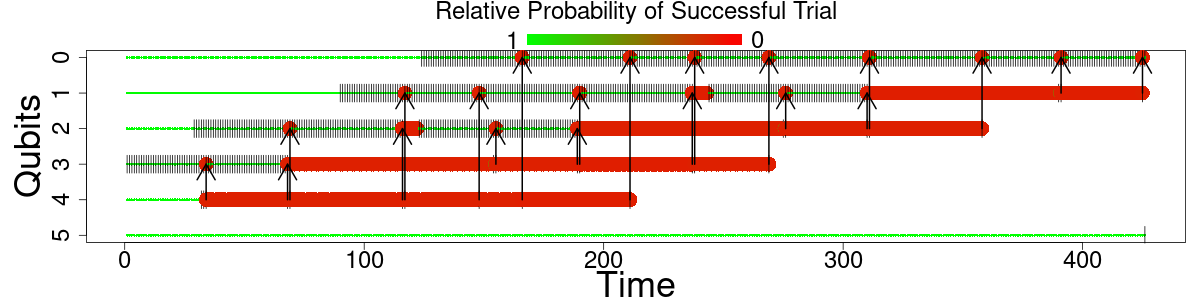
Figure 1: Noise sensitivity heatmap of a 6-qubit QPE alrogithm. Thin green lines represent insensitive; thick red lines, sensitive regions. Vertical lines correspond to single qubit gates. Arrows between qubits indicate two qubit interactions (i.e., gates). Horizontal lines terminate when the last operation on the respective qubit is complete, i.e., when the qubit is ready to be measured. Qubit 5 has no operations on it after state preparation. In our noise model, an error on a two-qubit gate affects both qubits.

The impact of a logical error on the success of a quantum program depends on when (at which cycle in the execution) and where (in which qubit) the error occurs [11]. We use statistical fault injection to characterize this behavior, where we inject errors at different locations at different times and track the propagation to the output of the program. Since we are working with QEC, we can assume that errors are restricted to X and Z errors (Y errors are a combination of X and Z errors). As a representative case study, we profile the Quantum Phase Estimation (QPE) algorithm, which incorporates the inverse Quantum Fourier Transform (QFT) as the main computational kernel. QPE is representative of algorithms a fault-tolerant quantum computer (i.e., a quantum computer which features QEC) is likely to run, and has important applications in quantum chemistry [8]. The input to QPE is a quantum state which has a phase angle difference between its constituent qubits. QPE detects this difference and produces a bitstring representing the angle. 6 qubits are large enough to show trends but small enough that visualization remains manageable. Patterns observed for 6 qubits hold for implementations of different qubit counts.

To produce the input quantum state, we perform noiseless state preparation. A sequence of controlled-phase gates are performed with qubits 0-4 as control and qubit 5 as the target. A noiseless QPE implementation acting on this state produces a single output bitstring with high probability ($>98\%$). This eases validation of the output.

To guarantee statistical significance, we run many individual fault injection experiments. In each experiment we inject an error to a single gate. We use Qiskit’s [2] depolarizing noise model with the error rate set to 100% (an error always occurs), where X, Z, and Y (both X and Z) errors are all equally likely. We evaluate the quality of the output by comparing the probability of successful trial (PST) to that of the noiseless output. As we set the input state so that there is only one correct answer, this metric becomes:

$$Relative\;PST=\frac{PST_{noisy}}{PST_{ideal}}$$ (5)

Figure 1 depicts the relative PST as a heatmap, to help visually inspect the significance of the error at each location and at each point in time. The x-axis is time; the y-axis, space (i.e., different qubits). Thick, red lines indicate sensitive regions. Notably, qubits become more sensitive after they act as the control qubit of a two-qubit gate. Intuitively, this is because the two-qubit gate entangles the qubits, merging two smaller states into a single, larger state. Once entangled in this manner, qubits remain sensitive until the end of the program.

4 Variable Strength QEC

Knowledge about the underlying noise sensitivity of a quantum program, both in time and space, makes variable strength (i.e., distance) QEC possible, where different logical qubits get protected by different levels (i.e., different code distances $d$) of QEC at different times. If a logical qubit is less susceptible to logical noise at a given point in time, it can survive with lighter weight QEC than more susceptible qubits.

We start by acknowledging a fundamental limitation to this idea. The logical error rate decreases exponentially with $d$. The physical qubit count increases with $d^{2}$. The time overhead increases linearly with $d$. Hence, we can save quadratic space and linear time, but risk exponential increases in error rates. This suggests that variable-strength QEC can easily backfire if applied too aggressively.

4.1 Success Rate as a Function of Code Distance

We estimate the probability of logical error on a qubit, $P_{L}$ from the physical error rate, $p$, for code distance $d$ with the analytical formula provided by Fowler et al. for surface codes [5]:

$$P_{L}\approx 0.03\times(p/0.0057)^{(d+1)/2}$$ (6)

The probability of successful trial (PST) is the probability of measuring the correct result at the end of the quantum program. With sufficiently high $d$, no logical errors would occur, and PST would be 1 (for quantum programs that have a single correct output). As $d$ decreases, PST decreases exponentially until it hits nearly 0. Where this decay occurs is a function of the physical error rate. Figure 2 shows the PST of QPE for different $d$ over a wide range of physical error rates. Higher $d$ values tolerate higher physical error rates by construction.

Using information from Figure 1, we know which logical qubits are more sensitive to noise, which we leverage to designate a variable distance QECC. We assign higher $d$ to the bold, red regions of Figure 1. Without loss of generality, we experiment with two-distance QECC: For example, $3,5$ is a QECC which uses $d=3$ on less susceptible qubits and $d=5$ on more susceptible qubits. The dashed lines in Figure 2 capture the variable (two-) distance QECC, which achieve resilience in-between their constituent code distances.

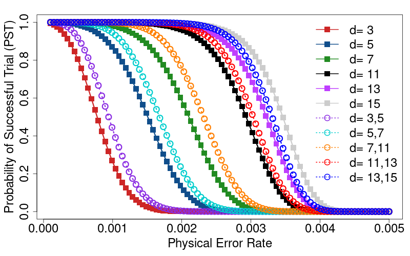
Figure 2: PST of QPE for different (including variable) code distances over a range of physical noise rates.

4.2 Time to Solution

We next combine the sensitivity information from Section 3.2 with the latency of each logic operation for a given code distance, to estimate the time to solution. As noted in Section 3.1, the time to solution corresponds to ${L}/{PST}$.

We estimate $PST$ by finding the probability of two events:

1. No logical error occurs

2. A single logical error occurs, but the output is the same as in the case of no error

These two probabilities combined provide a lower bound on $PST$. It is also possible that two or more logical errors occur and the output remains the same. However, counting these possibilities quickly becomes intractable because a total of $(N_{gates})^{N_{errors}}$ must be considered, where $N_{gates}$ is the number of quantum gates performed in the algorithm and $N_{errors}$ is the number of possible errors. Hence, in our analysis, two or more errors represent a failure.

A gate on a logical qubit with distance $d$ takes $d$ cycles to complete. Since the distance of each logical qubit is known throughout the program, we can easily find the corresponding latency, i.e., $L/PST$ which provides the time to solution as shown in Figure 3. It is noteworthy that the optimal code distance depends on the error rate. As intuition suggests, at low error rates lower code distances are preferable due to the lower overhead. However, as the error rate increases the codes begin to fail. Since error suppression is exponential, once the codes begin to fail, the reliability degrades dramatically and $P_{success}$ drops quickly. This necessitates a larger number of trials to obtain the correct solution, leading to a higher latency.

Each variable distance code is optimal within a range of error rates. For example, the QECC $d=3,5$ is optimal at error rates where $d=3$ begins to fail. $d=3,5$ can provide a faster solution than $d=5$, until it breaks down and $d=5$ becomes necessary to tolerate errors. However, interestingly, variable distance codes tend to provide the best solution for most error rates. When $d=3,5$ fails, $d=5,7$ is already preferable to $d=5$, as shown in Figure 3.

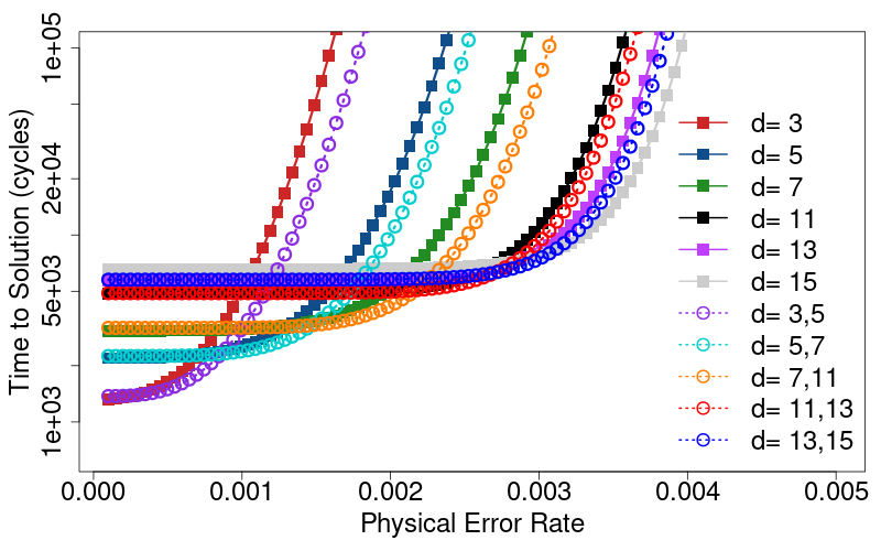
Figure 3: The time to solution for different code distances. Variable distance codes tend to provide the fastest solution for a given error rate.

4.3 Practical Considerations

While variable distance QECC looks promising, practical implementations can be challenging. In expected superconducting quantum architectures, for which surface codes are most appropriate, logical qubits are arranged next to each other in a two-dimensional lattice [7]. Non-uniform layouts incurred by expanding and contracting code distance (i.e., number of physical qubits per logical qubit) can result in wasted physical qubits. Additionally, latency of such state-of-the-art quantum computers is not limited by logic gates, but by the preparation of special quantum states required to perform specific operations (such as magic state distillation for T gates [10]). Hence, improvements in the gate latency for logical qubits (as enabled by variable strength QECC) may not be significant. Finally, quantum fault injection is tractable only for small circuits. Obtaining accurate sensitivity estimates for larger circuits poses a challenge.

5 Conclusion

Our profiling analysis based on statistical fault injection shows that quantum programs can be relatively insensitive to isolated logical errors, and that variable distance QECC can reduce the time to solution by exploiting the spatio-temporal differences in noise sensitivity. However, any decrease in code distance due to variable strength QECC comes with an exponential increase in logical failure rates, which may eliminate the benefits if not carefully administered.

References

- [1] Sergey Bravyi et al. Correcting coherent errors with surface codes. npj Quantum Information, 4(1):1–6, 2018.
- [2] Andrew Cross. The ibm q experience and qiskit open-source quantum computing software. In APS March Meeting Abstracts, volume 2018, pages L58–003, 2018.
- [3] Xinglei Dou and Lei Liu. A new qubits mapping mechanism for multi-programming quantum computing. In Proceedings of the ACM International Conference on Parallel Architectures and Compilation Techniques, pages 349–350, 2020.
- [4] Alexander Erhard et al. Characterizing large-scale quantum computers via cycle benchmarking. Nature communications, 10(1):1–7, 2019.
- [5] Austin G Fowler et al. Surface codes: Towards practical large-scale quantum computation. Physical Review A, 86(3):032324, 2012.
- [6] Clare Horsman et al. Surface code quantum computing by lattice surgery. New Journal of Physics, 14(12):123011, 2012.
- [7] Ali Javadi-Abhari et al. Optimized surface code communication in superconducting quantum computers. In Proceedings of the 50th Annual IEEE/ACM International Symposium on Microarchitecture, pages 692–705, 2017.
- [8] Benjamin P Lanyon et al. Towards quantum chemistry on a quantum computer. Nature chemistry, 2(2):106–111, 2010.
- [9] Gushu Li et al. Tackling the qubit mapping problem for nisq-era quantum devices. In Proceedings of the Twenty-Fourth International Conference on Architectural Support for Programming Languages and Operating Systems, pages 1001–1014, 2019.
- [10] Daniel Litinski. A game of surface codes: Large-scale quantum computing with lattice surgery. Quantum, 3:128, 2019.
- [11] Salonik Resch et al. A day in the life of a quantum error. IEEE Computer Architecture Letters, 2020.
- [12] Salonik Resch and Ulya R Karpuzcu. Benchmarking quantum computers and the impact of quantum noise. ACM Computing Surveys (CSUR), 54(7):1–35, 2021.
- [13] Peter Selinger. Newsynth: exact and approximate synthesis of quantum circuits. http://www.mathstat.dal.ca/ selinger/newsynth/.
- [14] Peter Selinger. Efficient clifford+ t approximation of single-qubit operators. arXiv preprint arXiv:1212.6253, 2012.
- [15] AM Steane. Introduction to quantum error correction. Philosophical Transactions of the Royal Society of London. Series A: Mathematical, Physical and Engineering Sciences, 356(1743):1739–1758, 1998.
- [16] Swamit S Tannu and Moinuddin K Qureshi. Not all qubits are created equal: a case for variability-aware policies for nisq-era quantum computers. In Proceedings of the Twenty-Fourth International Conference on Architectural Support for Programming Languages and Operating Systems, pages 987–999, 2019.
- [17] Ellis Wilson et al. Just-in-time quantum circuit transpilation reduces noise. In 2020 IEEE International Conference on Quantum Computing and Engineering (QCE), pages 345–355. IEEE, 2020.