Weisfeiler and Leman go Machine Learning: The Story so far

Abstract

In recent years, algorithms and neural architectures based on the Weisfeiler–Leman algorithm, a well-known heuristic for the graph isomorphism problem, have emerged as a powerful tool for machine learning with graphs and relational data. Here, we give a comprehensive overview of the algorithm’s use in a machine-learning setting, focusing on the supervised regime. We discuss the theoretical background, show how to use it for supervised graph and node representation learning, discuss recent extensions, and outline the algorithm’s connection to (permutation-)equivariant neural architectures. Moreover, we give an overview of current applications and future directions to stimulate further research.

Keywords: Machine learning for graphs, Graph neural networks, Weisfeiler–Leman algorithm, expressivity, equivariance

1 Introduction

Graph-structured data is ubiquitous across application domains, ranging from chemo- and bioinformatics (Barabasi and Oltvai, 2004; Jumper et al., 2021; Stokes et al., 2020) to computer vision (Simonovsky and Komodakis, 2017), and social network analysis (Easley and Kleinberg, 2010); see Figure 1 for an overview of application areas. We need techniques exploiting the rich graph structure and feature information within nodes and edges to develop successful machine-learning models in these domains. Due to the highly non-regular structure of real-world graphs, most approaches first generate a vectorial representation of each graph or node, so-called node or graph embeddings, respectively, to apply standard machine learning tools such as linear regression, random forests, or neural networks.

For successful (supervised) machine learning with graphs, node and graph embeddings need to address the following key challenges:

1. The graph embedding needs to be invariant to any permutation of the graph’s nodes, i.e., the output of the graph embedding must not change for different orderings.

2. In the case of node embeddings, the embedding needs to be (permutation-)equivariant to node orderings, i.e., reordering of the input results in a reordering of the output, accordingly.

3. The embeddings need to scale to large, real-world graphs and large sets thereof.

4. The embeddings need to consider attribute or label information, e.g., real-valued vectors attached to nodes and edges.

5. Finally, the embeddings need to generalize to unseen instances and ideally easily adapt or be robust to changes in the data distributions.

To address the above challenges, numerous approaches have been proposed in recent years—most notably, graph embedding approaches based on spectral techniques (Athreya et al., 2017; von Luxburg et al., 2008), graph kernels (Borgwardt et al., 2020; Kriege et al., 2020), and neural approaches (Chami et al., 2020; Gilmer et al., 2017; Scarselli et al., 2009) for both node and graph embeddings. Here, graph kernels are positive semi-definite functions, expressing a pairwise similarity between graphs. Especially, graph kernels based on the Weisfeiler–Leman algorithm (Weisfeiler and Leman, 1968), a graph comparison algorithm originally developed to address the graph isomorphism problem, see below, and corresponding neural architectures, known as graph neural networks (GNNs), have recently advanced the state-of-the-art in (semi-)supervised node-level and graph-level machine learning.

The ($1$-dimensional) Weisfeiler–Leman ($1$-WL) or color refinement algorithm is a well-known heuristic for deciding whether two graphs are isomorphic, i.e., exactly match structure-wise. Given an initial coloring or labeling of the nodes of both graphs, e.g., their degree or application-specific information, in each iteration, two nodes with the same label get different labels if the number of neighbors carrying a particular label is not equal, see Figure 2 for an illustration. If, after any iteration, the number of nodes annotated with a certain label is different in both graphs, the algorithm terminates, and we conclude that the two graphs are not isomorphic. This simple algorithm is already quite powerful in distinguishing non-isomorphic graphs (Babai and Kucera, 1979) and has been therefore applied in many areas, see, e.g., Grohe et al. (2014); Kersting et al. (2014); Zhang and Chen (2017), including graph classification (Shervashidze et al., 2011). On the other hand, it is easy to see that the algorithm cannot distinguish all non-isomorphic graphs (Cai et al., 1992). For example, it cannot distinguish graphs with different triangle counts, see Figure 3, or, in general, cyclic information (Arvind et al., 2015), which is an important feature in social network analysis (Milo et al., 2002; Newman, 2003) and chemical molecules. To increase the algorithm’s expressive power, it has been generalized from labeling nodes to $k$-tuples, defined over the set of nodes, leading to a more powerful graph isomorphism heuristic, denoted $k$-dimensional Weisfeiler–Leman algorithm ($k$-WL). The $k$-WL was investigated in-depth by the theoretical computer science community, see, e.g., Cai et al. (1992); Grohe (2017); Kiefer (2020a).

Shervashidze and Borgwardt (2009) first used the $1$-WL as a graph kernel, the so-called Weisfeiler–Lehman subtree kernel. The kernel’s idea is to compute the $1$-WL for a fixed number of steps, resulting in a color histogram or feature vector of color counts for each graph. Subsequently, taking the pairwise inner product between these vectors leads to a valid kernel function. Hence, the kernel measures the similarity between two graphs by counting common colors in all refinement steps. Similar approaches are popular in chemoinformatics for computing vectorial descriptors of chemical molecules (Rogers and Hahn, 2010).

Graph kernels were the primary approach for learning on graphs for several years, leading to new state-of-the-art results on many graph classification tasks. However, one limitation, in particular of the most efficient graph kernels, is that their feature vector representation corresponds to enumerating particular classes of subgraphs, and kernel computation corresponds to finding exactly matching pairs of these subgraphs in two graphs; thereby, partial similarities of subgraphs in two graphs may be missed. GNNs have emerged as a machine learning framework that aims to address these limitations. Primarily, they can be viewed as a neural version of the $1$-WL algorithm, where continuous feature vectors replace colors, and neural networks are used to aggregate over local node neighborhoods (Gilmer et al., 2017; Hamilton et al., 2017; Morris et al., 2019).

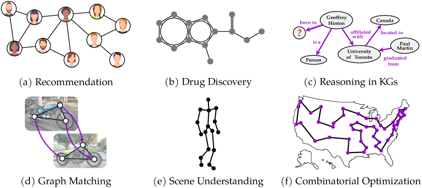
Figure 1: Example use cases for machine learning with graphs.

Recently, links between the two above paradigms emerged. Morris et al. (2019); Xu et al. (2019) showed that any possible GNN architecture cannot be more powerful than the $1$-WL in terms of distinguishing non-isomorphic graphs. Moreover, this line of work has been extended by deriving more powerful neural architectures, based on the $k$-WL (Maron et al., 2019c, a; Morris et al., 2019, 2020b), subsequently shown to be universal (Azizian and Lelarge, 2020; Keriven and Peyré, 2019; Maron et al., 2019c), i.e., being able to represent any continuous, bounded, invariant or equivariant function over the set of graphs.

1.1 Present Work

In this paper, we survey the application of the Weisfeiler–Leman algorithm to machine learning with graphs. To this end, we overview the algorithm’s theoretical properties and thoroughly survey graph kernel approaches based on the Weisfeiler–Leman paradigm. Subsequently, we also overview the recent progress in aligning the algorithm’s expressive power with equivariant neural networks, showing $1$-WL’s and $k$-WL’s equivalence to GNNs and more powerful higher-order GNNs, respectively. Alongside, we also survey works proving universality results of invariant and equivariant neural architectures for graphs. Moreover, we review recent efforts extending GNNs’ expressive power, their generalization abilities,w and exemplary applications of the algorithm’s use in machine learning with graphs. Finally, we discuss open questions and future research directions.

1.2 Related Work

In the following, we briefly discuss related work relevant to the present survey.

1.2.1 Graph Kernels

Intuitively, a graph kernel is a function measuring the similarity of a pair of graphs, see Section 2 for a formal definition and Mohri et al. (2012) as well as Shalev-Shwartz and Ben-David (2014) for an introduction to kernel functions for machine learning. Graph kernels were the dominant approach in machine learning for graphs, especially for graph classification with a relatively small number of graphs, for several years, see Borgwardt et al. (2020) and Kriege et al. (2020) for thorough surveys. Starting from the early 2000s, researchers proposed a plethora of graph kernels, e.g., based on shortest-paths (Borgwardt et al., 2005), random walks (Gärtner et al., 2003; Kang et al., 2012; Kashima et al., 2003; Sugiyama and Borgwardt, 2015; Kriege, 2022), small subgraphs (Shervashidze et al., 2009; Kriege and Mutzel, 2012), local neighborhood information (Costa and De Grave, 2010; Morris et al., 2017, 2020b; Shervashidze et al., 2011), Laplacian information (Kondor and Pan, 2016), and matchings (Fröhlich et al., 2005; Johansson and Dubhashi, 2015; Kriege et al., 2016; Nikolentzos et al., 2017; Woźnica et al., 2010).

1.2.2 Molecule Descriptors in Cheminformatics

The representation of small molecules by their structure to explain their chemical properties constitutes one of the early applications of graph theoretical concepts and has influenced modern graph theory (Biggs et al., 1986). Cheminformatics applies computer science methods to analyze chemical data and comprises several graph-theoretical and machine-learning problems. Finding a unique representation of a molecular structure corresponds to the graph canonization problem. Using the experimentally obtained bioactivity data of small molecules to predict the activity of untested molecules to find promising drug candidates is an instance of a graph classification or regression task. Therefore, it is not surprising that some techniques developed in cheminformatics are closely related to machine learning with graphs and the Weisfeiler–Leman method. We briefly review the developed methods and their relation to state-of-the-art techniques.

Morgan’s Algorithm

In 1965, Morgan (1965) proposed a method to generate unique identifiers for molecules, up to isomorphism, see Section 2, that was implemented at the Chemical Abstracts Service to index and provide chemistry-related information. To this end, the atoms are numbered canonically based on the atom and bond types and their structure. To increase efficiency, ambiguities are reduced by computing, for each node $v$, its connectivity value $\mathsf{ec}(v)$. Let $G=(V,E)$ be a (molecular) graph, initially we assign $\mathsf{ec}^{(1)}(v)=\deg(v)$ to every node $v$ in $V$, where $\deg(v)$ is the degree of $v$. Then, the values $\mathsf{ec}^{(i)}(v)$ are computed iteratively for $i\geq 2$ and all nodes $v$ in $V$ as

$$\mathsf{ec}^{(i)}(v)=\sum_{u\in N(v)}\mathsf{ec}^{(i-1)}(u),$$

until the number of different values no longer increases. For such an iteration $i$, $\mathsf{ec}^{(i-1)}(v)$ is the final extended connectivity of the node $v$. Razinger (1982) and Figueras (1993) independently observed that the extended connectivity values $\mathsf{ec}^{(i)}$ are equivalent to the row (or column) sums of the $i$th power of the adjacency matrix, which is equal to the number of walks of length $i$ starting at the individual nodes.

The general idea of encoding neighborhoods of increasing radius to make the descriptor more specific resembles the idea of the Weisfeiler–Leman algorithm. However, the connectivity value does not incorporate labels, i.e., atom and bond types, discards the values of $\mathsf{ec}^{(i-1)}(v)$ when computing $\mathsf{ec}^{(i)}(v)$, and loses information due to summation (Kriege, 2022).

Circular Fingerprints

In 1973, Adamson and Bush (1973) considered the task of automated classification of chemical structures by representing molecules by (chemical) fingerprints, i.e., a vectorial representation of a molecule. Today, fingerprints are a standard tool in cheminformatics used to determine molecular similarity, e.g., for classification, clustering, and similarity search in large chemical information systems (Rogers and Hahn, 2010). A fingerprint is a vector where each component counts the number of occurrences of certain substructures or merely indicates their presence or absence by a single bit. Often hashing is used to map substructures to the entries of a fixed-size fingerprint; see Daylight (2008). Fingerprints are typically compared using similarity measures for sets such as the Tanimoto coefficient, which satisfies the property of a kernel (Ralaivola et al., 2005); see Section 2. The substructures used may stem from a predefined set obtained either by applying data mining methods, using domain expert knowledge (Durant et al., 2002), or are enumerated directly from the molecular graph, e.g., all paths up to a given length.

Of particular interest to the present work is the class of circular fingerprints, where the substructures are the neighborhoods of each node with increasingly distant nodes added to the neighborhood. In this sense, this type of fingerprint is conceptually similar to Morgan’s algorithm and is occasionally also referred to as Morgan fingerprint. However, the key differences are that atom and bond types are encoded, the maximum radius is limited to a typically small value, and all the intermediate results for radii smaller than the maximum are retained (Rogers and Hahn, 2010). The earliest of these approaches goes back to so-called fragments reduced to an environment that is limited proposed in 1973 (Dubois, 1973; Dubois et al., 1987). Several variations of the approach have been proposed, e.g., atom environment fingerprints (Bender et al., 2004) and extended connectivity fingerprints (Rogers and Hahn, 2010). These fingerprints are widely used, and implementations are available in open-source and commercial software libraries such as RDKit and OpenEye GraphSim TK.

Duvenaud et al. (2015) proposed a neural extension of circular fingerprints introducing learnable parameters for encoding neighborhoods. This work as well as earlier techniques introduced in cheminformatics, e.g., Baskin et al. (1997); Kireev (1995); Merkwirth and Lengauer (2005), represent early instances of GNNs.

1.2.3 Graph Neural Networks

Recently, graph neural networks (GNNs) or message-passing neural networks (Gilmer et al., 2017; Scarselli et al., 2009) (re-)emerged as the most popular machine learning method for graph-structured input. Intuitively, GNNs can be viewed as a differentiable variant of the $1$-WL where colors are replaced with real-valued features and a neural network is used for neighborhood feature aggregation. By deploying a trainable neural network to aggregate information in local node neighborhoods, GNNs can be trained in an end-to-end fashion together with the classification or regression algorithm’s parameters, possibly allowing for greater adaptability and better generalization than the kernel counterpart of the classical $1$-WL algorithm, see Section 5.1 for details.

Notable instances of this architecture include Duvenaud et al. (2015); Hamilton et al. (2017); Veličković et al. (2018), which can be subsumed under the message passing framework introduced in Gilmer et al. (2017). In parallel, approaches based on spectral information were introduced in, e.g., Bruna et al. (2014); Defferrard et al. (2016); Gama et al. (2019); Kipf and Welling (2017); Levie et al. (2019); Monti et al. (2017). All of the above descend from early work in Baskin et al. (1997); Kireev (1995); Merkwirth and Lengauer (2005); Micheli (2009); Micheli and Sestito (2005); Scarselli et al. (2009); Sperduti and Starita (1997). Aligned with the field’s recent rise in popularity, there exists a plethora of surveys on recent advances in GNN techniques; some of the most recent ones include Chami et al. (2020); Wu et al. (2018); Zhou et al. (2018).

1.2.4 Equivariant Neural Networks

Input symmetries are frequently incorporated into learning models to construct efficient models. A prominent example is the translation invariance encoded by Convolutional Neural Networks (CNNs), particularly useful for image recognition tasks (LeCun et al., 2015). In the last few years, incorporating other types of symmetries in neural networks (Ravanbakhsh et al., 2017; Wood and Shawe-Taylor, 1996), e.g., a set structure where the output is invariant to the order of the input (Zaheer et al., 2017), became an important research direction. As with CNNs, the main idea is to construct neural networks as a composition of several (simple) equivariant building blocks, i.e., layers respecting the symmetry; see Section 6 for details. These networks were shown to reduce the number of free parameters and to improve efficiency and generalization.

One important research direction that follows this line of work is devising equivariant networks for learning on graphs, where, for most tasks, the specific order of nodes does not matter (Albooyeh et al., 2019; Keriven and Peyré, 2019; Kondor et al., 2018; Maron et al., 2019c, a, b; Puny et al., 2020; Ravanbakhsh, 2020). In Section 6, we discuss these models thoroughly and show that their expressive power is closely related to the Weisfeiler–Leman algorithm.

1.3 Structure of the Document

In Section 2, we fix notation and introduce basic concepts used throughout the present work. Section 3 introduces the $1$-WL, and its generalization, the $k$-WL, and gives an overview of its theoretical properties. In the next section, Section 4, we survey non-neural machine learning approaches leveraging the Weisfeiler–Leman algorithm, focusing on supervised graph classification. Section 5 introduces GNNs and their connection to the $1$-WL and investigates neural architectures beyond $1$-WL’s expressive power. Subsequently, Section 6 describes the recent progress in designing equivariant (higher-order) graph networks and their connection to the Weisfeiler–Leman hierarchy. Further, Section 8 outlines applications of Weisfeiler–Leman-based graph embeddings. Section 9 outlines open challenges and sketches future research directions. Finally, the last section acts as a conclusion.

2 Preliminaries

As usual, let $[n]=\{1,\dotsc,n\}\subset\mathbb{N}$ for $n\geq 1$, and let $\{\!\!\{\dots\}\!\!\}$ denote a multiset. A (undirected) graph $G$ is a pair $(V,E)$ with a finite set of nodes $V(G)$ and a set of edges $E(G)\subseteq\{\{u,v\}\subseteq V\mid u\neq v\}$. For notational convenience, we usually denote an edge $\{u,v\}$ in $E(G)$ by $(u,v)$ or $(v,u)$, and set $n=|V(G)|$ and $m=|E(G)|$. In case of a directed graph, the set of edges $E(G)\subseteq\{(u,v)\subseteq V^{2}\mid u\neq v\}$, i.e., $E(G)$ might not be symmetric and the edges $(u,v)$ and $(v,u)$ are considered distinct. A labeled graph $G$ is a triple $(V,E,l)$ with a label function $l\colon V(G)\cup E(G)\to\Sigma$, where $\Sigma$ is a subset of the natural numbers. Then $l(w)$ is a label of $w$ for $w$ in $V(G)\cup E(G)$. An attributed graph $G$ is a triple $(V,E,a)$ with an attribute function $a\colon V(G)\cup E(G)\to\mathbb{R}^{d}$ for $d>0$. Then $a(w)$ is an attribute or continuous label of a node or edge $w$ in $V(G)\cup E(G)$. We denote the set of all labeled or attributed graphs by $\mathcal{G}$. The neighborhood of $v$ in $V(G)$ is denoted by $N(v)=\{u\in V(G)\mid(v,u)\in E(G)\}$. Let $S\subseteq V(G)$, then the set $S$ induces a subgraph $(S,E_{S})$ with $E_{S}=\{(u,v)\in E(G)\mid(u,v)\in S\times S\}$. We say that two graphs $G$ and $H$ are isomorphic, denoted $G\simeq H$, if there exists an edge-preserving bijection (graph isomorphism) $\varphi\colon V(G)\to V(H)$, i.e., $(u,v)$ is in $E(G)$ if and only if $(\varphi(u),\varphi(v))$ is in $E(H)$. In the case of labeled graphs, we additionally require that $l(v)=l(\varphi(v))$ for $v$ in $V(G)$, similarly for edge labels. The graph isomorphism problem deals with deciding if two graphs are isomorphic or not. The isomorphism type $\tau(G)$ of a graph $G$ is the equivalence class induced by the (isomorphism) relation $\simeq$, i.e., $\tau(G)=\{H\in\mathcal{G}\mid G\simeq H\}$. A (graph) automorphism is an isomorphism from a graph to itself, i.e, $\varphi\colon V(G)\to V(G)$. A (graph) homomorphism is a map $\varphi\colon V(G)\to V(H)$ where $((\varphi(u),\varphi(v))$ in $E(H)$ if $(u,v)$ in $E(G)$. Note that $\varphi(v)=\varphi(w)$ for two distinct nodes $v$ and $w$ in $V(G)$ is permitted. Hence, as opposed to isomorphisms, homomorphisms need not to preserve non-edges, i.e., $(\varphi(u),\varphi(v))$ in $E(H)$ does not imply $(u,v)\in E(G)$.

Permutation-invariance and -equivariance

Let $n>0$, then $S_{n}$ denotes the set of permutations of $[n]$, i.e., the set of all bijections from $[n]$ to itself. Further, let $V(G)=[n]$, then for $\sigma$ in $S_{n}$, $G_{\sigma}=\sigma\cdot G$ where $V(G_{\sigma})=\{{\sigma(1)},\dots,{\sigma(n)}\}$ and $E(G_{\sigma})=\{({\sigma(i)},{\sigma(j)})\mid(v_{i},v_{j})\in E(G)\}$. That is, applying the permutation $\sigma$ reorders the nodes. Hence, for two isomorphic graphs $G$ and $H$, i.e., $G\simeq H$, there exists $\sigma$ in $S_{n}$ such that $\sigma\cdot G=H$.

Assuming that all graphs have $n$ nodes, a function $f\colon\mathcal{G}\to\mathbb{R}$ is invariant if $f(G)=f(\sigma\cdot G)$ for all graphs $G$ in $\mathcal{G}$ and all permutations $\sigma$ in $S_{n}$. More generally, given a set $\mathcal{X}$ on which $S_{n}$ acts, a function $f\colon\mathcal{G}\to\mathcal{X}$ is equivariant if $f(\sigma\cdot G)=\sigma\cdot f(G)$. In this paper, we mainly consider $\mathcal{X}=\mathbb{R}^{n}$ as a representation for node features. $S_{n}$ acts on this space by permuting the entries of the vector, i.e., $\sigma\cdot(x_{1},\ldots,x_{n})=(x_{\sigma^{-1}(1)},\ldots,x_{\sigma^{-1}(n)})$. Other options for $\mathcal{X}$ are discussed in Section 6.

Kernels

A kernel on a non-empty set $\mathcal{X}$ is a positive semi-definite, symmetric function $k\colon\mathcal{X}\times\mathcal{X}\to\mathbb{R}$. Equivalently, a function $k$ is a kernel if there is a feature map $\phi\colon\mathcal{X}\to\mathcal{H}$ to a Hilbert space $\mathcal{H}$ with an inner product $\langle\cdot,\cdot\rangle$, such that $k(x,y)=\langle\phi(x),\phi(y)\rangle$ for all $x$ and $y$ in $\mathcal{X}$. Then a positive semi-definite, symmetric function $\mathcal{G}\times\mathcal{G}\to\mathbb{R}$ is a graph kernel. Given two vectors $x$ and $y$ in $\mathbb{R}^{d}$, the linear kernel is defined as $k(x,y)=x^{\mathsf{T}}y$. Given a finite set $X=\{x_{1},\dots,x_{n}\}\subseteq\mathcal{X}$ and a kernel $k\colon\mathcal{X}\times\mathcal{X}\to\mathbb{R}$, the Gram matrix $M$ in $\mathbb{R}^{n\times n}$ contains the kernel values for each pair of elements of the set $X$, i.e., $M_{ij}=k(x_{i},x_{j})$; see, e.g., Mohri et al. (2012), for details.

3 The Weisfeiler–Leman Method

Figure 2: Illustration of $1$-WL’s relabeling procedure. The brown, lower-left node gets updated based on the colors of its neighbors.

As mentioned in Section 1, the $1$-WL or color refinement is a simple heuristic for the graph isomorphism problem, originally proposed in Weisfeiler and Leman (1968). Intuitively, the algorithm tries to determine if two graphs are non-isomorphic by iteratively coloring or labeling nodes. Given an initial coloring or labeling of the nodes of both graphs, e.g., their degree or application-specific information, in each iteration, two nodes with the same label get different labels if the number of identically labeled neighbors is not equal. If, after some iterations, the number of nodes annotated with a specific label is different in both graphs, the algorithm terminates, and we conclude that the two graphs are not isomorphic. It is easy to see that the algorithm cannot distinguish all non-isomorphic graphs; see Figure 3 and Cai et al. (1992). Nonetheless, it is a powerful heuristic that can successfully test isomorphism for a broad class of graphs (Babai and Kucera, 1979), see Section 3.3 for an in-depth discussion on the algorithm’s properties.

Formally, let $G=(V,E,l)$ be a labeled graph, in each iteration, $i>0$, the $1$-WL computes a node coloring $C^{1}_{i}\colon V(G)\to\mathbb{N}$, which depends on the coloring of the neighbors. That is, in iteration $i>0$, we set

$$C^{1}_{i}(v)=\textsc{Relabel}\Big{(}\!\big{(}C^{1}_{i-1}(v),\{\!\!\{C^{1}_{i-1}(u)\!\mid\!u\in\!N(v)\!\}\!\!\}\big{)}\!\Big{)},$$ (1)

where Relabel injectively maps the above pair to a unique natural number, which has not been used in previous iterations. Viewed differently, $C^{1}_{i-1}$ induces a partitioning of a graph’s node set, which is further refined by $C^{1}_{i}$. In iteration $0$, the coloring $C^{1}_{0}=l$ or a constant value if no labeling is provided.

That is, in each iteration, the algorithm computes a new color for a node based on the colors of its neighbors; see Figure 2 for an illustration. Hence, after $k$ iterations the color of a node $v$ captures some structure of its $k$-hop neighborhood, i.e., the subgraph induced by all nodes reachable by walks of length at most $k$.

To test if two graphs $G$ and $H$ are non-isomorphic, we run the above algorithm in “parallel” on both graphs. If the two graphs have a different number of nodes colored $c$ in $\mathbb{N}$ at some iteration, the $1$-WL concludes that the graphs are not isomorphic. Moreover, if the number of colors between two iterations, $i$ and $(i+1)$, does not change, i.e., the cardinalities of the images of $C^{1}_{i}$ and $C^{1}_{i+1}$ are equal or, equivalently,

$$C^{1}_{i}(v)=C^{1}_{i}(w)\iff C^{1}_{i+1}(v)=C^{1}_{i+1}(w),$$

for all nodes $v$ and $w$ in $V(G)$, the algorithm terminates. For such $i$, we define the stable coloring $C^{1}_{\infty}(v)=C^{1}_{i}(v)$ for $v$ in $V(G)$. The stable coloring is reached after at most $\max\{|V(G)|,|V(H)|\}$ iterations (Grohe, 2017); see Section 3.3 for further bounds on the algorithm’s running time.

(a) Example 1

(b) Example 2

Figure 3: Examples of two graphs (denoted by $\blacksquare$ and $\blacksquare$) that cannot be distinguished by the $1$-WL.

3.1 The k-dimensional Weisfeiler–Leman Algorithm

Due to the shortcomings of the $1$-WL or color refinement in distinguishing non-isomorphic graphs, several researchers (Babai, 1979, 2016; Immerman and Lander, 1990), devised a more powerful generalization of the former, today known as the $k$-dimensional Weisfeiler–Leman algorithm. In the literature, there exist two variants of the algorithm, which differ slightly in the way they aggregate information. The variant we describe below is often denoted folklore $k$-dimensional Weisfeiler–Leman algorithm ($k$-FWL) in the machine learning literature, e.g., see Maron et al. (2019a); Morris et al. (2019). We follow this convention to be aligned with papers in the machine learning literature. We also define the other variant, named oblivious $k$-WL ($k$-OWL), see Section 3.2.

Intuitively, to surpass the limitations of the $1$-WL, the $k$-FWL colors subgraphs instead of a single node. More precisely, given a graph $G$, it colors tuples from $V(G)^{k}$ for $k\geq 1$ instead of nodes. By defining a neighborhood between these tuples, we can define a coloring similar to the $1$-WL. Formally, let $G$ be a graph, and let $k\geq 2$. Moreover, let $\mathbf{v}$ be a tuple in $V(G)^{k}$, then $G[\mathbf{v}]$ is the subgraph induced by the components of $\mathbf{v}$, where the nodes are labeled with integers from $\{1,\dots,k\}$ corresponding to indices of $\mathbf{v}$. In each iteration $i\geq 0$, the algorithm, similarly to the $1$-WL, computes a coloring $C^{k}_{i}\colon V(G)^{k}\to\mathbb{N}$. In the first iteration ($i=0$), two tuples $\mathbf{v}$ and $\mathbf{w}$ in $V(G)^{k}$ get the same color if the map $v_{i}\mapsto w_{i}$ induces an isomorphism between $G[\mathbf{v}]$ and $G[\mathbf{w}]$. Now, for $i>0$, $C^{k}_{i+1}$ is defined by

$$C^{k}_{i+1}(\mathbf{v})=\textsc{Relabel}\Big{(}\!(C^{k}_{i}(\mathbf{v}),M_{i}(\mathbf{v}))\!\Big{)},$$ (2)

where the multiset

$$M_{i}(\mathbf{v})=\{\!\!\{(C^{k}_{i}(\phi_{1}(\mathbf{v},w)),\dots,C^{k}_{i}(\phi_{k}(\mathbf{v},w)))\mid w\in V(G)\}\!\!\}$$ (3)

and

$$\phi_{j}(\mathbf{v},w)=(v_{1},\dots,v_{j-1},w,v_{j+1},\dots,v_{k}).$$

That is, $\phi_{j}(\mathbf{v},w)$ replaces the $j$-th component of the tuple $\mathbf{v}$ with the node $w$. Hence, two tuples are adjacent or $j$-neighbors (with respect to a node $w$) if they are different in the $j$th component (or equal, in the case of self-loops). Again, we run the algorithm until convergence, i.e.,

$$C^{k}_{i}(\mathbf{v})=C^{k}_{i}(\mathbf{w})\iff C^{k}_{i+1}(\mathbf{v})=C^{k}_{i+1}(\mathbf{w}),$$

for all $\mathbf{v}$ and $\mathbf{w}$ in $V(G)^{k}$ holds, and call the partition of $V(G)^{k}$ induced by $C^{k}_{i}$ the stable partition. For such $i$, we define $C^{k}_{\infty}(\mathbf{v})=C^{k}_{i}(\mathbf{v})$ for $\mathbf{v}$ in $V(G)^{k}$. Hence, two tuples $\mathbf{v}$ and $\mathbf{w}$ with the same color in iteration $(t-1)$ get different colors in iteration $t$ if there exists $j$ in $[k]$ such that the number of $j$-neighbors of $\mathbf{v}$ and $\mathbf{w}$, respectively, colored with a certain color is different. The algorithm then proceeds analogously to the $1$-WL.

By increasing $k$, the algorithm gets more powerful in distinguishing non-isomorphic graphs, i.e., for each $k\geq 1$, there are non-isomorphic graphs distinguished by the ($k+1$)-WL but not by the $k$-WL (Cai et al., 1992). See Section 3.3 for a thorough discussion of the algorithm’s properties and limitations.

Figure 4: Illustration of $k$-FWL’s neighborhood definition for $k=3$. The $3$-tuple $(w,b,c)$ is a $1$-neighbor of the $3$-tuple $(a,b,c)$, while $(a,v,c)$ is a $2$-neighbor of the $3$-tuple $(a,b,c)$.

3.2 Oblivious k-WL

In the literature, e.g., Grohe (2000), there exists a variation of Equation 3 that leads to a slightly less powerful algorithm using the coloring $C^{k,*}_{i}\colon V(G)^{k}\to\mathbb{N}$. For $i>0$, $C^{k,*}_{i+1}$ is defined by

$$C^{k,*}_{i+1}(\mathbf{v})=\textsc{Relabel}\Big{(}\!(C^{k,*}_{i}(\mathbf{v}),M^{*}_{i}(\mathbf{v}))\!\Big{)},$$ (4)

where $M_{i}(\mathbf{v})$ in Equation 2 is replaced by

$$M^{*}_{i}(\mathbf{v})=\big{(}\{\!\!\{C^{k,*}_{i}(\phi_{1}(\mathbf{v},w))\mid w\in V(G)\}\!\!\},\dots,\{\!\!\{C^{k,*}_{i}(\phi_{k}(\mathbf{v},w))\mid w\in V(G)\}\!\!\}\big{)}.$$ (5)

Following Grohe (2021), we call the resulting algorithm oblivious $k$-WL ($k$-OWL).

It holds that the $1$-OWL and $2$-OWL have the same expressive power and that the $(k+1)$-OWL has the same expressive power as the $k$-FWL for $k\geq 2$ (Grohe, 2021). The reason the $k$-OWL has a lower expressive power than the $k$-FWL is due to the different way they aggregate colors. That is, the $k$-FWL, see Equation 3, groups colors of $k$-tuples according to the replaced node. For example, by that, the $k$-FWL is able to reconstruct if there is an edge between the two exchanged nodes; see Grohe (2021) for details.

3.3 Theoretical Properties

The Weisfeiler–Leman algorithm constitutes one of the earliest approaches to isomorphism testing (Weisfeiler and Leman, 1968; Weisfeiler, 1976). The $1$-dimensional version is an essential building block of the individualization-refinement approach to graph isomorphism testing (McKay, 1981), forming the basis of almost all practical graph isomorphism solvers. Higher-dimensional versions have been heavily investigated by the theory community over the last few decades, see, e.g., Cai et al. (1992); Grohe (2017); Kiefer (2020b); Otto (1997). For logarithmic $k$, the $k$-dimensional WL algorithm is an essential building block of Babai’s isomorphism algorithm (Babai, 2016) running in quasipolynomial time, i.e., its running time is in $2^{\mathcal{O}(\log^{c}n)}$ for a constant $c>0$. In the following, we overview the Weisfeiler–Leman algorithm’s theoretical properties, stressing relevance for machine learning with graphs when possible.

Expressive Power

We say that the $k$-FWL or $k$-OWL distinguishes two graphs $G$ and $H$ if their color histograms differ, i.e., there is some color $c$ in the image of $C^{k}_{\infty}$ such that $G$ and $H$ have different numbers of node tuples of color $c$. Furthermore, $k$-FWL or $k$-OWL identifies a graph $G$ if it distinguishes $G$ from all graphs not isomorphic to $G$.

As previously mentioned, Figure 3 shows a pair of simple, non-isomorphic graphs that are not distinguished by the $1$-WL. Still, it is likely that the $1$-WL will distinguish any two random graphs. It can be shown that the $1$-WL almost surely identifies all graphs. That is, the probability that the $1$-WL identifies a graph chosen uniformly at random from the class of all $n$-node graphs goes to $1$ as $n$ goes to infinity. The above result follows from an old result due to Babai et al. (1980) stating that with probability greater than $1-\sqrt[7]{\nicefrac{{1}}{{n}}}$, in a random $n$-node graph, all nodes get different colors after just two iterations of running the $1$-WL. The result was subsequently refined and extended; see Babai and Kucera (1979); Czajka and Pandurangan (2008); Karp (1979); Lipton (1978). While the $1$-WL cannot distinguish any two regular graphs with the same number of nodes and degree, Bollobás (1982) showed that the $2$-FWL identifies almost all $d$-regular graphs for every degree $d$. However, the $2$-FWL cannot distinguish any two strongly regular graphs with the same parameters, see, e.g., Grohe and Neuen (2021), and Figure 5. For $k\geq 3$, it is much harder to find non-isomorphic graphs that are not distinguished by the $k$-FWL, resulting in the seminal paper by Cai et al. (1992). For every $k$, they constructed non-isomorphic graphs $G_{k}$ and $H_{k}$, with the number of nodes in ${\mathcal{O}}(k)$, that are not distinguished by the $k$-FWL. These graphs can be distinguished by the $(k+1)$-FWL. Hence with increasing dimension, the expressive power of the Weisfeiler–Leman algorithm increases. This hierarchy of more powerful algorithms was later leveraged to devise more powerful graph neural networks, see Sections 5 and 6.

While the construction outlined in Cai et al. (1992) shows the limitations of the Weisfeiler–Leman algorithm, the algorithm is still powerful, in combination with the structural restrictions of the graphs. The WL dimension of a graph $G$ is the least $k$ such that $k$-FWL identifies $G$. Clearly, every $n$-node graph is identified by $(n-1)$-FWL and thus has WL-dimension at most $n-1$. In a far-reaching result, Grohe (2012, 2017) proved that for every $h>0$ there is a $k>0$ such that all graphs, excluding some $h$-node graph as a minor, have WL-dimension at most $k$. Here a graph $H$ is a minor of a graph $G$ if $H$ is isomorphic to a graph obtained from $G$ by deleting nodes or edges and by contracting edges. Since planar graphs exclude the complete 5-node graph $K_{5}$ as a minor, planar graphs have a bounded WL dimension. Similarly, the theorem shows that graphs of bounded genus or bounded treewidth and also more esoteric topologically constrained graphs, for example, graphs that can be embedded into 3-space in such a way that no cycle is knotted (Robertson et al., 1993), have bounded WL dimension. Other graphs known to have bounded WL dimensions are interval graphs (Evdokimov et al., 2000) and graphs of bounded rank width (Grohe and Neuen, 2019). For some of these classes, explicit bounds on the WL dimension are known. Most notably, planar graphs have WL dimension at most $3$ (Kiefer et al., 2019). This result has relevance for many applications that involve planar graphs. For example, a large portion of molecules is known to be planar (Horváth et al., 2010; Yamaguchi et al., 2003). Moreover, Kiefer et al. (2015); Arvind et al. (2015) gave a complete characterization of the graphs of WL dimension $1$. See Kiefer (2020a, b) for thorough overviews of the algorithm’s expressive power.

Figure 5: Two non-isomorphic strongly regular graphs (denoted by $\blacksquare$ and $\blacksquare$) with parameters $(16,6,2,2)$ that cannot be distinguished by $2$-FWL: the line graph of $K_{4,4}$ (left) and the Shrikhande graph (right). Figure adapted from Grohe and Neuen (2021).

Complexity

While a naive implementation of the $1$-WL requires (at least) quadratic time ${\mathcal{O}}(nm)$, where $n$ is the number of nodes and $m$ the number of edges of the input graph, Cardon and Crochemore (1982) proved that the stable coloring $C^{1}_{\infty}$ can be computed in almost linear time $O(n+m\log n)$; also see Paige and Tarjan (1987). Berkholz et al. (2017) proved that this is optimal within a large class of natural partitioning algorithms that includes all known algorithms for $1$-WL. Immerman and Lander (1990) generalized the almost-linear $1$-WL algorithm to the $k$-FWL and proved that the stable coloring $C^{k}_{\infty}$ can be computed in time $O(k^{2}n^{k+1}\log n)$. For every fixed $k\geq 1$, the problem of deciding whether two graphs are distinguished by $k$-FWL is PTIME-complete under logspace reductions (Grohe, 1999). Hence, it is unlikely that there are fast parallel algorithms computing the stable coloring.

Related to these complexity-theoretic results is the question of how many iterations the $k$-FWL needs to reach the stable coloring. A trivial upper bound is $n^{k}-1$ because, in each iteration, the number of colors increases, and a partition of a set of size $n^{k}$ has at most $n^{k}$ classes. Kiefer and McKay (2020) devised several infinite classes of graphs where $1$-WL needs the maximum number of $n-1$ iterations. Quite surprisingly, Lichter et al. (2019) proved an upper bound of $O(n\log n)$ on the number of iterations of $2$-FWL, a subquadratic upper bound was already known from Kiefer and Schweitzer (2016). No non-trivial upper bound is known for the $k$-FWL with $k\geq 3$, and the best known lower bound for all $k$ is linear (Fürer, 2001).

Connections With Other Areas

A particularly nice feature of the Weisfeiler–Leman algorithm is that it has several characterizations in terms of seemingly unrelated concepts from logic, algebra, and combinatorics. Here, the logical characterization turned out to be instrumental in proving several of the expressive power results mentioned above. Specifically, Cai et al. (1992) showed that two graphs are indistinguishable by the $k$-FWL if and only if they satisfy the same sentences of the logic $\textsf{C}^{k+1}$, the $(k+1)$-variable fragment of first-order logic extended by counting quantifiers.

Tinhofer (1986, 1991) derived an equivalence between $1$-WL’s inability to distinguish two non-isomorphic graphs and a system of linear equations having a real solution. By considering the relaxation $L$ of an integer linear program for the graph isomorphism problem, he showed that two non-isomorphic graphs cannot be distinguished by the $1$-WL if and only if $L$ has a real solution, also known as fractional isomorphism. The authors of Atserias and Maneva (2013); Grohe and Otto (2015); Malkin (2014) later lifted the above equivalence to the $k$-FWL by considering a slight variation $L^{k}_{-}$ of the linear program $L^{k}$ of the $k$th level of the Sherali-Adams hierarchy for the linear program $L$. For $k\geq 2$, they showed that two non-isomorphic graphs cannot be distinguished by the $k$-FWL if and only if the $L^{k}_{-}$ has a real solution. Similar results were obtained for systems of polynomial equations (Berkholz and Grohe, 2017), algebraic proof systems (Berkholz and Grohe, 2015; Grädel et al., 2019), semidefinite programming (Atserias and Ochremiak, 2018; O’Donnell et al., 2014), and non-signaling quantum isomorphisms (Atserias et al., 2019). Finally, Kersting et al. (2014) pointed out a close relationship between the $1$-WL and the Franke-Wolfe algorithm for convex optimization.

Dvorák (2010), see also Dell et al. (2018), showed a connection between $k$-FWL’s expressive power and homomorphism counts. Given two graphs $F$ and $G$, $\textsf{hom}(F,G)$ denotes the number of (graph) homomorphisms between the graphs $F$ and $G$. Given a set of graphs $\mathcal{F}$, the homormorphism number vector $\overrightarrow{\textsf{hom}}(\mathcal{F},G)=(\textsf{hom}(F,G))_{F\in\mathcal{F}}$ contains the number of homomorphisms between any graph in $\mathcal{F}$ and $G$. Dvorák (2010) showed that the $k$-FWL does not distinguish a pair of non-isomorphic graphs if and only if their homomorphism number vectors are equal for the set of graphs with treewidth of at most $k$.

4 Non-neural Methods for Machine Learning Based on the Weisfeiler–Leman Algorithm

In the following, we review applications of the Weisfeiler–Leman method for machine learning focusing on graph kernels. Hence, this section mainly deals with (supervised) graph-level prediction tasks, e.g., graph classification, where node and edge labels are often absent. Starting from the Weisfeiler–Leman subtree kernel (Shervashidze et al., 2011), we thoroughly survey graph kernels based on the Weisfeiler–Leman method.

4.1 Weisfeiler–Lehman Subtree Kernel

(a) Graph with refined labels

(b) $1$-WL color histogram

Figure 6: Illustration of the feature vector (color histogram) computed by the Weisfeiler–Lehman subtree kernel. From left to right, smaller circles represent colors from previous iterations. Large circles represent the $1$-WL colors after three iterations. Initially, all nodes are colored gray.

The Weisfeiler–Lehman subtree kernel (Shervashidze and Borgwardt, 2009) constitutes the earliest approach to leverage the $1$-WL as a graph kernel, inspiring many follow-up works. The primary idea is to compute the $1$-WL for $h\geq 0$ iterations, resulting in a coloring $C^{1}_{i}\colon V(G)\to\Sigma_{i}$ for each iteration $i$, where $\Sigma_{i}$ is a finite subset of the natural numbers, i.e., $\Sigma_{i}\subset\mathbb{N}$. Notice that the image of the coloring changes in every iteration, depending on the multiset generated by $1$-WL. For $i=0$, we set $\Sigma_{0}=\Sigma$, i.e., the original node label alphabet. In each iteration, we compute a feature vector or color histogram $\phi_{i}(G)$ in $\mathbb{R}^{|\Sigma_{i}|}$ for each input graph $G$.

Each component $\phi_{i}(G)_{c}$ counts the number of occurrences of nodes labeled by $c$ in $\Sigma_{i}$. With the ordering of $\Sigma_{i}$ being fixed and known beforehand—which is equivalent to knowing the label alphabet $\Sigma$ in advance—the vector $\phi_{i}(G)$ can be padded with zeroes if necessary. The overall feature vector $\phi_{\text{WL}}(G)$ is then defined as the concatenation of the feature vectors of all $h$ iterations, i.e.,

$$\phi_{\text{WL}}(G)=\big{[}\phi_{0}(G),\dots,\phi_{h}(G)\big{]}.$$ (6)

See Figure 6 for an illustration of the feature vector $\phi_{\text{WL}}(G)$. We obtain the corresponding kernel for $h$ iterations as

$$k_{\text{WL}}(G,H)=\langle\phi_{\text{WL}}(G),\phi_{\text{WL}}(H)\rangle,$$ (7)

where $\langle\cdot,\cdot\rangle$ denotes the standard inner product or linear kernel. Hence, the Weisfeiler–Lehman subtree kernel sums the number of node pairs with the same color over all refinement steps. Note that more powerful kernels may also replace the linear kernel, such as the RBF kernel (see, e.g., Togninalli et al. (2019)).

The running time for a single feature vector computation is in ${\mathcal{O}}(hm)$ and ${\mathcal{O}}(Nhm+N^{2}hn)$ for the calculation of the Gram matrix for a set of $N$ graphs (Shervashidze et al., 2011), under the assumption that a linear-time perfect hashing function is available for computing the coloring. Here, $n$ and $m$ denote the maximum number of nodes and edges over all $N$ graphs, respectively. Hence, the algorithm scales well to large graphs and data sets and can be used together with linear SVMs (Chang et al., 2008) to avoid the quadratic overhead of computing the Gram matrix.

4.2 Variations of the Weisfeiler–Lehman Subtree Kernel

The subtree kernel gives rise to many variations, focusing on different aspects of a graph. Shervashidze et al. (2011) describe two variations, which we will briefly discuss.

The first is the Weisfeiler–Lehman edge kernel, instead of counting the color of nodes, it computes a feature vector $\phi^{\text{E}}_{i}(G)$, counting edges whose incident nodes have identical colors. Two such feature vectors can then be compared using a linear kernel. As for the node-based subtree kernel described above, the overall kernel expression for the edge-based Weisfeiler–Leman kernel is an inner product of feature vectors concatenated over each iteration,

$$k_{\text{WL}}^{\text{E}}(G,H)=\langle\phi^{\text{E}}(G),\phi^{\text{E}}(H)\rangle,$$

where

$$\phi^{\text{E}}(G)=[\phi^{\text{E}}_{0}(G),\dotsc,\phi^{\text{E}}_{h}(G)].$$

The second variation is obtained similarly to the first one but employs a shortest-path kernel (Borgwardt and Kriegel, 2005) in iteration $i$. This results in a feature vector of the form $\phi^{\text{SP}}(G)=[\phi^{\text{SP}}_{0}(G),\dotsc\phi^{\text{SP}}_{h}(G)]$. Each $\phi^{\text{SP}}_{i}(G)$ consists of triples $(\sigma,\tau,l)$, with $\sigma$ and $\tau$ in $\Sigma_{i}$ denoting the labels of the start and end node of the shortest path, respectively, and $l$ denoting its length, which can either be an edge count or incorporate additional edge weights of the graph. Again, such a kernel can be expressed as an inner product of concatenated feature vectors,

$$k_{\text{WL}}^{\text{SP}}(G,H)=\langle\phi^{\text{SP}}(G),\phi^{\text{SP}}(H)\rangle.$$

The advantage of both of these variations is their flexibility—more complicated kernels can be easily accommodated, making it possible to capture additional information on the edge labels of a graph.

4.3 Matching-based Kernels

The Weisfeiler–Lehman subtree kernel sums the number of node pairs with the same color over all refinement steps. Other approaches to graph similarity match node pairs colored by the Weisfeiler–Leman method and obtain a graph kernel from an optimal assignment (Kriege et al., 2016) or the Wasserstein distance (Togninalli et al., 2019), which we overview below.

(a) Graph with refined labels

(b) Hierarchy representing the refinement

Figure 7: Hierarchical node partitioning from the 1-WL. Smaller circles represent colors from previous iterations. Large circles represent the $1$-WL colors after three iterations. Initially, all nodes are colored gray.

Kernel Based on Optimal Assignments

Given two sets $A$ and $B$ with $|A|=|B|=n$ and a similarity matrix $S$ in $\mathbb{R}^{n\times n}$, where $S_{ij}$ is the similarity of $A_{i}$ and $B_{j}$ in $A$ and $B$, respectively, the (linear) assignment problem aims to find

$$\operatorname{LAP}(A,B)=\max_{P\in\mathcal{P}_{n}}\langle P,S\rangle\quad\text{with}\quad\mathcal{P}_{n}=\left\{P\in\{0,1\}^{n\times n}:P\mathbf{1}=\mathbf{1},P^{\top}\mathbf{1}=\mathbf{1}\right\},$$ (8)

where $\mathcal{P}_{n}$ is the set of $n\times n$ permutation matrices, $\mathbf{1}$ is a vector of “ones,” and $\langle\cdot,\cdot\rangle$ is the Frobenius inner product, i.e., the element-wise product of two matrices.

Hence, we can compare graphs by computing an optimal assignment between their nodes according to a similarity function defined on their nodes, augmenting the smaller graph with dummy nodes if necessary. The first graph kernel based on this idea was proposed by Fröhlich et al. (2005). The similarities on the nodes are determined by arbitrary kernels taking the node attributes and their neighborhood into account. However, in this case, Equation 8 not always yields a positive semidefinite kernel (Vert, 2008). Kriege et al. (2016) showed that when the similarity matrix $S$ is obtained from a specific class of base kernels derived from a hierarchy, the value of the optimal assignment is guaranteed to yield a positive semidefinite kernel. Such base kernels can be obtained from the Weisfeiler–Leman method based on the following observation. The Weisfeiler–Leman method produces a hierarchy on the nodes of a set of graphs, where the $i$th level consists of nodes for each color in the refinement step $i+1$ with an artificial root at level $0$. The parent-child relationships are given by the refinement process, where the root has the initial node labels as children, see Figure 7. This hierarchy gives rise to the base kernel

$$k(u,v)=\sum_{i=0}^{h}k_{\delta}(C^{1}_{i}(u),C^{1}_{i}(v)),\quad k_{\delta}(x,y)=\begin{cases}1,\ x=y\\ 0,\ x\neq y\end{cases}$$ (9)

on the nodes. The kernel counts the number of iterations required to assign different colors to the nodes and reflects the extent to which the nodes have a structurally similar neighborhood. For example, in Figure 7, we have $k(a,f)=2$, because the nodes $a$ and $f$ are contained in the same subtree on level $0$ and $1$, but not on the deeper levels. The optimal assignment kernel with this base kernel is referred to as the Weisfeiler–Lehman optimal assignment kernel. It is computed in linear time from the hierarchy of the base kernel and achieves better accuracy results in many classification experiments compared to the Weisfeiler–Lehman subtree kernel. Moreover, the hierarchy can be endowed with weights, which can be optimized via multiple kernel learning (Kriege, 2019).

Kernel Based on Wasserstein Distances

A related idea to establish an optimal matching is employed by the so-called Wasserstein distance (or earth mover’s distance, optimal transport distance). Let $A$ and $B$ in $\mathbb{R}^{n}_{+}$ with entries that sum to the same value and $D$ in $\mathbb{R}^{n\times n}_{+}$ a distance matrix, the Wasserstein distance

$$W(A,B)=\min_{T\in\Gamma(A,B)}\langle T,D\rangle\quad\text{with}\quad\Gamma(A,B)=\left\{T\in\mathbb{R}^{n\times n}_{+}:T\mathbf{1}=A,T^{\top}\mathbf{1}=B\right\},$$ (10)

where $\Gamma(A,B)$ is the set of so-called transport plans. Intuitively, an element $D_{ij}$ of the matrix $D$ specifies the cost of moving one unit from $i$ to $j$. Then, the Wasserstein distance is the minimum cost required to transform $A$ into $B$.

Togninalli et al. (2019) derived valid kernels from the Wasserstein distance by using a distance on the nodes obtained from the Weisfeiler–Leman method according to

$$d(u,v)=\frac{1}{h+1}\sum_{i=0}^{h}\rho(C^{1}_{i}(u),C^{1}_{i}(v)),\quad\rho(x,y)=\begin{cases}1,\ x\neq y\\ 0,\ x=y.\end{cases}$$ (11)

Equation 11 can be regarded as a normalized distance associated with the kernel of Equation 9. For example, in Figure 7, we have $d(a,f)=\nicefrac{{1}}{{2}}$, since the nodes $a$ and $f$ are in different subtrees in two of the four levels. The Wasserstein distance $W(A,B)$ of Equation 10 using Equation 11 on the nodes is then combined with a distance substitution kernel (Haasdonk and Bahlmann, 2004), specifically a variant of the Laplacian kernel. The resulting kernel was shown to be positive semidefinite. For graphs with continuous attributes, Togninalli et al. (2019) proposed an extension of the Weisfeiler–Leman method replacing discrete colors with real-valued vectors. Then, the ground costs of the Wasserstein distance are obtained from the Euclidean distance between these vectors. In this case, it is not guaranteed that the resulting kernel is positive semidefinite. To circumvent this issue, Togninalli et al. (2019) proposed using a Kreĭn SVM (Loosli et al., 2016), i.e., an SVM that is capable of handling indefinite kernels.

4.4 Continuous Attributes

Due to its origin in graph isomorphism testing, the Weisfeiler–Leman algorithm initially only applies to (discretely) labeled graphs. Hence, it is not clear how to extend the algorithm to graphs with continuous attributes, i.e., graphs whose nodes and edges exhibit high-dimensional feature vectors in some $\mathbb{R}^{d}$. Over the years, there have been multiple noteworthy approaches to address this problem, two of which we briefly discuss and describe below.

The chronologically first approach is due to Orsini et al. (2015) and describes graph invariant kernels. The overarching idea is to extend existing graph kernels so that they are able to capture continuous attributes. This necessitates the definition of a graph invariant. We will provide an abstract definition first and discuss a more concrete example based on $1$-WL later on. A function $\mathcal{I}\colon\mathcal{G}\to\mathbb{R}$ is a graph invariant if it maps isomorphic graphs $G$ and $H$ to the same element, i.e., $\mathcal{I}(G)=\mathcal{I}(H)$ if $G\simeq H$. Similarly, a function $\mathcal{L}\colon V(G)\to\mathbb{R}$ is a node invariant if it assigns labels to the nodes of a graph $G$ such that they are preserved under any isomorphism $\varphi$, i.e., $\mathcal{L}(v)=\mathcal{L}(\varphi(v))$ for all $v$ in $V(G)$. Since every node invariant can be phrased as a specific graph invariant, we will subsequently not distinguish between node and graph invariants. Given a graph invariant, we can define a generic kernel function of the form

$$k_{\text{GIK}}(G,H)=\sum_{v\in V(G)}\sum_{v^{\prime}\in V(H)}\mathrm{w}(v,v^{\prime})\cdot k_{\text{Attr}}(v,v^{\prime}),$$

where $\mathrm{w}(v,v^{\prime})$ denotes a function that assesses the similarity between vertices $v$ and $v^{\prime}$ (Orsini et al. (2015) suggest using a graph invariant function; as we shall subsequently see, $1$-WL can be employed here), and $k_{\text{Attr}}(v,v^{\prime})$ denotes a kernel between node attributes. A simple choice for $k_{\text{Attr}}(v,v^{\prime})$ is an RBF kernel. As for $\mathrm{w}(v,v^{\prime})$, this function can be realized using, among others, the $1$-WL, by setting

$$\mathrm{w}(v,v^{\prime})=\sum_{i=0}^{h}\left|\{v\mid c_{l}^{(i)}(v)=c_{l}^{(i)}(v^{\prime})\}\right|,$$ (12)

i.e., the number of times two nodes are being assigned the same color during the 1-WL refinement scheme with $h$ iterations. While only being one specific choice for $\mathrm{w}(v,v^{\prime})$, this demonstrates the utility of $1$-WL beyond the use of a similarity measure itself. In effect, the $1$-WL can also provide more fundamental insights into the structure of a graph.

The second approach is due to Morris et al. (2016). Its fundamental idea is to employ the $1$-WL scheme to assess the similarity of labeled graphs, which are, in turn, obtained by employing a hashing scheme. The hashing scheme transforms continuous node attributes into discrete ones, while the 1-WL scheme facilitates the comparison of such labeled graphs. Formally, given a family $\mathcal{H}$ of hash functions, the hash graph kernel takes the form

$$k_{\text{HGK}}(G,H)=\frac{1}{J}\sum_{j=1}^{J}k_{\text{WL}}(h_{j}(G),h_{j}(H)),$$ (13)

where $h_{j}\colon\mathbb{R}^{d}\to\mathbb{N}$ refers to a hash function from $\mathcal{H}$. This representation once again demonstrates the versatility of the $1$-WL framework. Multiple hash functions are used in the previous equation to ensure that continuous attributes are represented sufficiently. Originally, the authors propose to use locality-sensitive hashing schemes (Datar et al., 2004), but other choices are also possible. The running time of a hash graph kernel evaluation can be upper-bounded by the running time of the $1$-WL scheme, i.e., $\mathcal{O}(hm)$, and the complexity of the hashing scheme $\mathcal{O}(t_{h})$, leading to an overall complexity of $\mathcal{O}(J(hm+t_{h}))$. For a fixed number of iterations $J$ and under the (reasonable) assumption that the hash function is no more complex than calculating $1$-WL feature vectors, the hash graph kernel complexity is thus asymptotically no higher than the complexity of $1$-WL.

In addition to these principled approaches, other works also provide variants of the $1$-WL scheme to target continuous attributes. The work by Togninalli et al. (2019), for instance, which we discussed in Section 4.3, can also be applied to graphs with continuous attributes. Its formulation does not give rise to a positive semidefinite kernel, thus necessitating the use of a special SVM for training (Loosli et al., 2016). Moreover, due to its reliance on Wasserstein calculations, its complexity is considerably higher with $\mathcal{O}(n^{3}\log n)$ for evaluating the kernel between two graphs $G$ and $H$, where $n$ refers to the maximum number of nodes in the two graphs.

4.5 Kernels Based on the k-OWL

Morris et al. (2017) proposed the first graph kernel based on the $k$-OWL. Essentially, the kernel computation works the same way as in the $1$-dimensional case, i.e., a feature vector is computed for each graph based on color counts. To make the algorithm more scalable, the author resorted to coloring all subgraphs on $k$ nodes instead of all $k$-tuples, resulting in a less powerful algorithm (Abboud et al., 2021). Moreover, the authors proposed only considering a subset of the original neighborhood to exploit the sparsity of the underlying graph. Formally, let $G$ be a graph, for a given $k\geq 2$, they consider all $k$-element subsets $[V(G)]^{k}$ over $V(G)$. Let $s=\{s_{1},\dotsc,s_{k}\}$ be a $k$-set in $[V(G)]^{k}$, then they define the global neighborhood of $s$ as

$$N(s)=\{t\in[V(G)]^{k}\mid|s\cap t|=k-1\}\,.$$

That is, two $k$-element subsets are neighbors if they are different in one element. The local neighborhood  $N_{L}(s)$ consists of all $t$ in $N(s)$ such that $(v,w)$ in $E(G)$ for the unique $v$ in $s\setminus t$ and the unique $w$ in $t\setminus s$. The coloring $[V(G)]^{k}\to\mathbb{N}$ is then defined analogously to Equation 1 using the local neighborhood. Intuitively, the global neighborhood of a $k$-element subset $s$ consists of all other $k$-element subsets $s$ such that we can go from $s$ to $t$ by replacing exactly one node. The local neighborhood requires that these replaced nodes are adjacent. For example, in Figure 4, the subset $\{a,c,v\}$ is in the local neighborhood of $\{a,b,c\}$ because the nodes $b$ and $v$ are adjacent.

Further, they offered a sampling-based algorithm to speed up the kernel computation for large graphs approximating it in constant time, i.e., independent of the number of nodes and edges, with an additive approximation error. Finally, they show empirically that the proposed kernel beats the Weisfeiler–Leman subtree kernel on a subset of tested benchmark data sets.

Similarly to the above work, Morris et al. (2020b) also proposed graph kernels based on $k$-OWL. Again, for scalability, they only consider a subset of the original neighborhood. However, they consider $k$-tuples and prove that a variant of their method is slightly more powerful than the $k$-OWL, see Section 3.2 while taking the original graph’s sparsity into account. That is, instead of Equation 3, it uses

$$\begin{split}M^{\delta}_{i}(\mathbf{v})=\big{(}\{\!\!\{C^{k,\delta}_{i}(\phi_{1}(\mathbf{v},w))\mid w\in N(v_{1})\}\!\!\},\dots,\{\!\!\{C^{k,\delta}_{i}(\phi_{k}(\mathbf{v},w))\mid w\in N(v_{k})\}\!\!\}\big{)}.\end{split}$$

Hence, two tuples $\mathbf{v}$ and $\mathbf{w}$ are local $i$-neighbors if the nodes $v_{i}$ and $w_{i}$ are adjacent in the underlying graph, effectively exploiting the sparsity of the underlying graph. Consequently, the labeling function is defined by

$$C^{k,\delta}_{i+1}(\mathbf{v})=\textsc{relabel}(C^{k,\delta}_{i}(\mathbf{v}),M^{\delta}_{i}(\mathbf{v})).$$

This local version is incomparable to the $k$-OWL in terms of distinguishing non-isomorphic graphs. That is, there exist pairs of non-isomorphic graphs that the above local variant can distinguish while the $k$-OWL can not and vice versa. However, the authors devised a variant of the above coloring function, with the same asymptotic running time as the above, that is more powerful than the $k$-OWL in distinguishing non-isomorphic graphs. Empirically, they show that this variant of the $k$-OWL achieves a new state-of-the-art across many standard benchmark data sets (Morris et al., 2020a) while being several orders of magnitude faster than the $k$-OWL.

Finally, Morris et al. (2022) introduced a more scalable variant of the above local version by omitting certain $k$-tuples. Concretely, they proposed the local $(k,s)$-WL, which only considers $k$-tuples inducing at most $s$ connected components, and studied its expressive power.

4.6 Other Kernels Based on the 1-WL

Figure 8: A brief overview of the topology-based extension of the $1$-WL scheme, introduced by Rieck et al. (2019). After obtaining the $1$-WL multiset labels, they are used to define a metric on the input graph $G$, turning it into a weighted graph $G^{\prime}$. This weighted graph is then used to determine the topological relevance of each node, which is subsequently used to reweight the WL feature vector $\phi_{\text{WL}}$.

The general utility of the $1$-WL scheme made it a natural building block in other algorithms and a central element in others. To guide the subsequent discussion, we briefly expand on the $\mathcal{R}$-convolution framework (Haussler, 1999), which to this date underlies most graph kernel approaches either implicitly or explicitly. This framework provides a way to construct kernels to compare structured objects by decomposing them according to a set of agreed-upon substructures, such as shortest paths. Two objects (e.g., graphs) are then compared by defining a kernel on their respective substructures. Many existing graph kernels can be rephrased as kernels based on the $\mathcal{R}$-convolution framework, see, e.g., Borgwardt et al. (2020) or Kriege et al. (2020), for recent surveys that provide in-depth discussions of this framework.

As an example of an algorithm in which the $1$-WL scheme constitutes a building block, Yanardag and Vishwanathan (2015a) employed it in its capacity to enumerate substructures, with the expressed goal to obtain “smoothed” variants of existing graph kernels. These are graph kernels built on a less rigid version of the $\mathcal{R}$-convolution framework that supports partial matches between substructures. The smoothed variant of $1$-WL demonstrates superior predictive performance than its “rigid” variant but with higher computational costs. In a similar vein, Yanardag and Vishwanathan (2015b) describe how to modify existing graph kernels such that they decompose graphs into their substructures. These substructures are then treated as sentences (in the natural language processing sense) arising from some vocabulary. This perspective enables the re-weighting of structures based on co-occurrence counts, resulting in a generic kernel formulation

$$k_{\text{DGK}}(G,H)=\phi(G)\mathcal{D}\phi^{\top}(H),$$

where $\phi(\cdot)$ refers to a feature vector representation of a graph kernel and $\mathcal{D}$ denotes a diagonal matrix containing substructure weights. The re-weighted “deep” version of $1$-WL also performs slightly better than the unweighted one, but the computational requirements are again substantially higher.

As an example of the second type of approach, where $1$-WL constitutes a critical element, we briefly summarize a method by Rieck et al. (2019). This paper is motivated by the observation that $1$-WL on its own cannot capture arbitrary topological features, such as cycles, in graphs (see Section 3.3 or Grohe and Kiefer (2021) for more details and see Figure 3 for a simple example of this). Making use of recent advances in topological data analysis, see Hensel et al. (2021) for a current survey, Rieck et al. (2019) used the “persistence”, i.e., a type of multi-scale measure for assessing the relevance of topological structures in a graph $G$, to provide weights for the individual dimensions of $1$-WL feature vectors $\phi_{\text{WL}}(G)$. This amounts to imbuing the label counts with additional information about their topological relevance in terms of connected components and cycles. For instance, if a set of labels often occurs as a part of a pronounced cycle in the graph, its weight will be larger than that of a label that only contributes marginally to the overall topology of a graph. Figure 8 illustrates the overall workflow. The $1$-WL is used to generate multiset labels, from which a weighted graph is obtained via a multiset distance metric. Topological features of the graph are then calculated, resulting in a topological relevance score for each node or edge.

Figure 9: Illustration of GNN’s neighorbood aggregation.

Rieck et al. (2019) empirically demonstrated that the inclusion of cycles can boost the performance of the $1$-WL, particularly for molecular data sets. Moreover, they also proved that it is possible to rephrase the $1$-WL scheme as a specific instance of a general topological relabeling scheme based on graph distances. In essence, the original $1$-WL feature vectors are obtained by using the uniform graph metric, which assigns all edges the same value. Zhang et al. (2018) devised a pooling method for GNNs, see below, inspired by the $1$-WL histogram construction.

5 Connections to Graph Neural Networks

In the following, we overview the connections between the Weisfeiler–Leman hierarchy, see Section 3, and neural networks for graphs, specifically GNNs. We introduce GNNs and their connection to the $1$-WL and overview GNN architectures overcoming the limitation of the $1$-WL.

5.1 GNNs and the 1-WL algorithm

Intuitively, GNNs or message-passing neural networks compute a vectorial representation, i.e., a $d$-dimensional vector, representing each node in a graph by aggregating information from neighboring nodes; see Figure 9 for an illustration. Formally, let $G=(V,E,l)$ be a labeled graph with initial node features $f^{(0)}\colon V(G)\rightarrow\mathbb{R}^{1\times d}$ that are consistent with $l$. That is, each node $v$ is annotated with a feature $f^{(0)}(v)$ in $\mathbb{R}^{1\times d}$ such that $f^{(0)}(u)=f^{(0)}(v)$ if $l(u)=l(v)$, e.g., a one-hot encoding of the the labels $l(u)$ and $l(v)$. Alternatively, $f^{(0)}(v)$ can be an arbitrary real-valued feature vector or attribute of the node $v$, e.g., physical measurements in the case of chemical molecules. A GNN architecture consists of a stack of neural network layers, i.e., a composition of parameterized functions. Each layer aggregates local neighborhood information, i.e., the neighbors’ features, around each node and then passes this aggregated information on to the next layer.

GNNs are often realized as follows (Morris et al., 2019). In each layer, $t>0$, we compute node features

$$f^{(t)}(v)=\sigma\Big{(}f^{(t-1)}(v)\cdot W^{(t)}_{1}+\,\sum_{\mathclap{w\in N(v)}}\,\,f^{(t-1)}(w)\cdot W_{2}^{(t)}\Big{)}$$ (14)

in $\mathbb{R}^{1\times e}$ for $v$, where $W_{1}^{(t)}$ and $W_{2}^{(t)}$ are parameter matrices from $\mathbb{R}^{d\times e}$ , and $\sigma$ denotes an entry-wise non-linear function, e.g., a sigmoid or a ReLU function. Following Gilmer et al. (2017); Scarselli et al. (2009), one may also replace the sum defined over the neighborhood in the above equation by an arbitrary, differentiable function, and one may substitute the outer sum, e.g., by a column-wise vector concatenation. Thus, in full generality a new feature $f^{(t)}(v)$ is computed as

$$f^{W_{1}}_{\text{merge}}\Big{(}f^{(t-1)}(v),f^{W_{2}}_{\text{aggr}}\big{(}\{\!\!\{f^{(t-1)}(w)\mid w\in N(v)\}\!\!\}\big{)}\!\Big{)},$$ (15)

where $f^{W_{2}}_{\text{aggr}}$ aggregates over the multiset of neighborhood features and $f^{W_{1}}_{\text{merge}}$ merges the node’s representations from step $(t-1)$ with the computed neighborhood features. Both $f^{W_{1}}_{\text{aggr}}$ and $f^{W_{2}}_{\text{merge}}$ may be arbitrary differentiable functions and, by analogy to Equation 14, we denote their parameters as $W_{1}$ and $W_{2}$, respectively. To adapt the parameters $W_{1}$ and $W_{2}$ of Equations 14–15, they are optimized in an end-to-end fashion, usually via a variant of stochastic gradient descent, e.g., Kingma and Ba (2015), together with the parameters of a neural network used for classification or regression.

Concurrently with Xu et al. (2019), Morris et al. (2019) showed that any GNN’s expressive power is upper bounded by the $1$-WL in terms of distinguishing non-isomorphic graphs. That is, given two non-isomorphic graphs, for any choice of functions $f^{W_{1}}_{\text{merge}}$ and $f^{W_{2}}_{\text{aggr}}$ and parameters $W_{1}$ and $W_{2}$, the GNN is not able to learn node features distinguishing two graphs if the $1$-WL cannot distinguish them. Let $W^{(t)}$ denote the set of weights up to layer $t$. Formally, we can write the above down as follows.

Theorem 1 (Morris et al., 2019; Xu et al., 2019)

Let $G=(V,E,l)$ be a labeled graph. Then for all $t\geq 0$ and for all choices of initial colorings $f^{(0)}$ consistent with $l$, and weights $W^{(t)}$,

$$C^{1}_{t}(u)=C^{1}_{t}(v)\text{ implies }f^{(t)}(u)=f^{(t)}(v),$$

for all nodes $u$ and $v$ in $V(G)$.

On the positive side, Morris et al. (2019) proved that there exists a sequence of parameter matrices ${W}^{(t)}$ such that GNNs have exactly the same expressive power in terms of distinguishing non-isomorphic (sub-)graphs as the $1$-WL algorithm by deriving injective variants of the functions $f^{W_{1}}_{\text{merge}}$ and $f^{W_{2}}_{\text{aggr}}$.

This equivalence in expressive power even holds for the simple architecture of (14), provided one chooses the encoding of the initial labeling $l$ in such a way that different labels are encoded by linearly independent vectors (Morris et al., 2019).

Theorem 2 (Morris et al., 2019)

Let $G=(V,E,l)$ be a labeled graph. Then for all $t\geq 0$, there exists a sequence of weights ${W}^{(t)}$, and a GNN architecture such that

$$C^{1}_{t}(u)=C^{1}_{t}(v)\text{ if and only if }f^{(t)}(u)=f^{(t)}(v),$$

for all nodes $u$ and $v$ in $V(G)$.

Similarly, (Xu et al., 2019) derived the Graph Isomorphism Network (GIN) layer and showed that it has the same expressive power as the $1$-WL in terms of distinguishing non-isomorphic graphs. Concretely, the GIN layer updates a feature of node $v$ at layer $t$ as

$${f}^{t}(v)=\text{MLP}\Big{(}(1+\varepsilon)\cdot f^{t-1}(v)+\sum_{w\in N(v)}f^{t-1}(w)\Big{)},$$

where MLP is a standard multi-layer perceptron, and $\varepsilon$ is a learnable scalar value. See Grohe (2021) for an in-depth discussion of both approaches. Further, Aamand et al. (2022) devised an improved analysis using randomization. In summary, we arrive at the following insight: Any possible graph neural network architecture can be at most as powerful as the $1$-WL in terms of distinguishing non-isomorphic graphs. A GNN architecture has the same expressive power as the $1$-WL if the functions $f^{W_{1}}_{\text{merge}}$ and $f^{W_{2}}_{\text{aggr}}$ are injective.

Barceló et al. (2020) further tightened the relationship between $1$-WL and GNNs by deriving a GNN architecture that has the same expressive power as the logic $\textsf{C}^{2}$, see Section 3.3. Moreover, Geerts et al. (2020) showed a connection between the $1$-WL and the GCN layer introduced in Kipf and Welling (2017).

5.2 Neural Architectures Beyond 1-WL’s Expressive Power

In the following, we overview some recent works overcoming the limitations of the $1$-WL.

Higher-order Architectures

Morris et al. (2019) proposed the first GNN architecture that overcame the limitations of the $1$-WL. Specifically, they introduced so-called $k$-GNNs, which work by learning features over the set of subgraphs on $k$ nodes instead of nodes by defining a notion of the neighborhood between these subgraphs. Formally, let $G$ be a graph, for a given $k$, they consider all $k$-element subsets $[V(G)]^{k}$ over $V(G)$. Let $s=\{s_{1},\dotsc,s_{k}\}$ be a such $k$-element subset, an element in $[V(G)]^{k}$, then they define the neighborhood of $s$ as

$$N(s)=\{t\in[V(G)]^{k}\mid|s\cap t|=k-1\}.$$

That is, two $k$-element subsets are neighbors if they are different in one element. The local neighborhood  $N_{L}(s)$ consists of all $t$ in $N(s)$ such that $(v,w)$ in $E(G)$ for the unique $v$ in $s\setminus t$ and the unique $w$ in $t\setminus s$. The global neighborhood $N_{G}(s)$ then is defined as $N(s)\setminus N_{\text{L}}(s)$. Hence, the neighborhood definition equals the one of Section 4.5

Based on this neighborhood definition, one can generalize most GNN layers for node embeddings, e.g., the one from Equation 14, to more powerful subgraph embeddings. Given a graph $G$, in each layer $t$, a $d$-dimensional real-valued feature for a subgraph $s$ can be computed as

$$f^{t}_{k}(s)=\sigma\Big{(}f^{t-1}_{k}(s)\cdot W_{1}^{t}+\sum_{u\in N_{L}(s)\cup N_{G}(s)}f^{t-1}_{k}(u)\cdot W_{2}^{t}\Big{)}.$$ (16)

At initialization, i.e., layer $t=0$, the feature of the $k$-element subset $s$ is set to a one-hot encoding of the (labeled) isomorphism type of the graph $G[s]$ induced by $s$, possibly enhanced by application-specific node and edge features. The authors resort to sum over the local neighborhood in the experiments for better scalability and generalization, showing a significant boost over standard GNNs on a quantum chemistry benchmark data set (Ramakrishnan et al., 2014; Wu et al., 2018).

Moreover, rather than starting at $k$-node subgraphs, Morris et al. (2019) also proposed a hierarchical variant of the layer in Equation 16 that combines the information of the $k$-node subgraph’s isomorphism types with learned vectorial representations of $(k-1)$-node subgraphs using a $(k-1)$-GNN. That is, rather than simply using one-hot indicator vectors as initial feature inputs in a $k$-GNN, they proposed a hierarchical variant of $k$-GNN that uses the features learned by a $(k-1)$-dimensional GNN, in addition to the (labeled) isomorphism type, as the initial features, i.e.,

$$f^{(0)}_{k}(s)=\sigma\Big{(}\big{[}f^{\text{iso}}(s),\sum_{u\subset s}f^{\,(T_{k-1})}_{k-1}(u)\Big{]}\cdot W_{k-1}\Big{)},$$

for some $T_{k-1}>0$, where $W_{k-1}$ is a matrix of appropriate size, $f^{\text{iso}}$ is a neural network that learns a vectorial representation of the subset $s$ based on a one-hot encoding of the (labeled) isomorphism type of the graph $G[s]$ induced by $s$, and square brackets denote column-wise matrix concatenation. Hence, the features are recursively learned from dimensions $1$ to $k$ in an end-to-end fashion. Further, Morris et al. (2020b) devised a neural version of the local version of the $k$-OWL, see Section 4.5, inheriting its expressive power.

Unique Node Identifiers

Vignac et al. (2020) extended the expressive power of GNNs, by using unique node identifiers, generalizing the message-passing scheme proposed by Gilmer et al. (2017), see Equation 15, by computing and passing matrix features instead of vector features. Formally, given an $n$-node graph, each node $i$ maintains a matrix $U_{i}$ in $\mathbb{R}^{n\times c}$ for $c>0$, denoted local context, where the $j$-th row contains the node $i$’s vectorial representation of node $j$. At initialization, each local context $U_{i}$ is set to a one-hot vector in $\mathbb{R}^{n\times 1}$. Now at each layer $l$, similar to the above message-passing framework, the local context is updated as

$$U_{i}^{(l+1)}=u^{(l)}\left(U_{i}^{(l)},\tilde{U}_{i}^{(l)}\right)\in\mathbb{R}^{n\times c_{l+1}}\quad\text{with}\quad\tilde{U}_{i}^{(l)}=\phi\left(\left\{m^{(l)}({U}_{i}^{(l)},{U}_{j}^{(l)},{e}_{ij})\right\}_{j\in N(i)}\right),$$

where $u^{(l)},m^{(l)}$, and $\phi$ are update, message, and aggregation functions, respectively, to compute the updated local context, and $e_{ij}$ denotes the edge feature shared by node $i$ and $j$. The authors studied the expressive power of the above architecture, showing that it is more powerful than 1-WL, and proposed more scalable alternative variants of the above architecture. Moreover, they derived conditions for equivariance. Finally, promising results on standard benchmark data sets are reported.

To derive more powerful graph representations, Murphy et al. (2019a, b), inspired by Yarotsky (2018), proposed relational pooling. To increase the expressive power of GNN layers, they averaged over all permutations of a given graph. Formally, let $G$ be a graph, then a representation

$$f(G)=\frac{1}{|V(G)|!}\sum_{\pi\in\Pi}g(A_{\pi,\pi},[F_{\pi},I_{|V|}])$$ (17)

is learned, where $\Pi$ denotes all possible permutations of the rows and columns of the adjacency matrix of the graph $G$. Here, $A_{\pi,\pi}$ permutes the rows and columns of the adjacency matrix $A$ according to the permutation $\pi$ in $\Pi$, similarly $F_{\pi}$ permutes the rows of the feature matrix $F$. Moreover, $g$ is a (possibly permutation-sensitive) function to compute a vectorial representation of the graph $G$, based on $A_{\pi,\pi}$ and $F_{\pi}$, $I_{|V|}$ is the $|V|\times|V|$ identity matrix, and $[\cdot,\cdot]$ denotes column-wise matrix concatenation. The authors showed that the above architecture is more powerful in terms of distinguishing non-isomorphic graphs than the $1$-WL, and proposed sampling-based techniques to speed up the computation. If the underlying model $g$ has maximal expressive power, e.g., an MLP, this model can be shown to distinguish all non-isomorphic graphs. Further, Keriven et al. (2021) studied unique node identifiers in the context of large random graphs.

Randomized Node Labels

Murphy et al. (2019a); Sato et al. (2020); Abboud et al. (2021) showed that adding random features, e.g., sampled from the standard uniform distribution, concatenated to the initial node features, enhances the expressive power of GNNs. Specifically, Sato et al. (2020) showed that adding random features to the initial features of the GIN layer of Section 5.1 improves their ability to randomly approximate the solution of common combinatorial optimization problems, e.g., minimum dominating set problem and maximum matching problem, over standard GNNs. Abboud et al. (2021) investigated the universality, see Section 6.2 below, of such architectures. They showed that adding random features to GNNs results in universality for the class of invariant functions on graphs with high probability. Dasoulas et al. (2020) obtained similar universality results also leveraging random colorings.

Homomorphism- and Subgraph-based Approaches

Bouritsas et al. (2023) extended the expressive power of GNNs by enhancing them with subgraph information. Specifically, they fix a set of small subgraphs $\mathcal{F}$ of given graph $G$. For each node $v$ in $V(G)$ and each subgraph $F$ in $\mathcal{F}$, they compute the node’s role in the subgraph and add this information to the node’s feature. That is, formally, they compute the automorphism type of node $v$ concerning the subgraph $F$. Similarly, they add information based on the edge automorphism type. Theoretically, they derived conditions under which the enhanced GNNs become more powerful than the $1$-WL, based on the choice of the set of subgraphs $\mathcal{F}$. By relying on homomorphism counts, Barceló et al. (2021) analyzed under which conditions adding more subgraphs leads to added expressivity and studied the expressive power of the resulting architectures compared to the $k$-FWL. Moreover, NT and Maehara (2020) directly leveraged the connection between homomorphism counts and the $k$-FWL hierarchy, see Section 3.3, and proved universality results for such architectures.

Subgraph-enhanced Approaches

Recently, another type of subgraph-based approach to enhance GNNs’ expressive power emerged; see, e.g., Bevilacqua et al. (2021); Cotta et al. (2021); Li et al. (2020); Papp et al. (2021); Thiede et al. (2021); You et al. (2021); Wijesinghe and Wang (2022); Zhao et al. (2021). These approaches enhanced the expressive power of GNNs by representing graphs as multi-sets of subgraphs and applying GNNs to these subgraphs. The subgraphs are obtained by removing, extracting, or marking (small) subgraphs to allow GNNs to leverage more structural patterns within the given graph, essentially breaking symmetries induced by the GNNs’ local aggregation function. We henceforth refer to these approaches as subgraph-enhanced GNNs.

For example, Cotta et al. (2021) derived a more powerful graph representation based on ideas inspired by the graph reconstruction conjecture (Bondy, 1991). They showed that removing single vertices and deploying GNNs on the resulting subgraphs leads to more powerful GNN architectures. Moreover, they showed that such architectures can be made more powerful by removing several vertices simultaneously, distinguishing graphs the $2$-FWL cannot. Papp et al. (2021) proposed a similar approach. Instead of removing all vertices, the authors proposed to remove vertices randomly. Papp and Wattenhofer (2022) compared these approaches’ expressive power to the subgraph-based approaches; see the previous paragraph.

You et al. (2021) proposed, for each node $v$, to extract its $k$-disc, i.e., the graph induced by all nodes at a distance at most $k$ from node $v$, and assigned a unique marking to node $v$. Each message passing iteration used two aggregation functions with distinct parameters. One function aggregates features around node $v$ and the other aggregates around all other subgraph nodes. They showed that this architecture can, e.g., count the number of cycles starting at node $v$, predict the clustering coefficient, or distinguish random $d$-regular graphs. Hence, making it strictly more powerful than standard GNNs. Sandfelder et al. (2021) enhanced GNN’s expressive power by proposing an architecture performing message passing within each node’s ego network, i.e., the subgraph induced by a node and its neighbors, and across ego networks. The authors show that such architecture can distinguish the graphs of Figure 3. Similarly, Zhang and Li (2021) proposed to make GNNs more powerful by extracting the $k$-hop neighborhood around each node and applying a standard GNN on top. The resulting node representations for each subgraph are then pooled together to learn a single representation for each node. Under certain assumptions, the authors showed that such an architecture can distinguish regular graphs.

Moreover, Bevilacqua et al. (2021) generalized several ideas discussed above and proposed a framework in which each graph is represented as a subset of its subgraphs and processed using an equivariant architecture based on the Deep Sets for Symmetric elements architecture (Maron et al., 2020) and message-passing neural networks. The authors showed that several simple subgraph selection policies, e.g., edge removal, ego networks, or node removal, generate more powerful GNNs, and derived equivalent WL-like procedures. In follow-up work, Frasca et al. (2022) presented a novel symmetry analysis for several of the approaches mentioned above (Bevilacqua et al., 2021; You et al., 2021; Cotta et al., 2021; Zhao et al., 2021), for the common case in which subgraphs are selected in one-to-one correspondence with nodes (for example, by deletion of nodes, node marking, or extraction of ego networks). Based on this symmetry analysis, they were able to link subgraph-enhanced GNNs with previously studied equivariant models for graphs (Maron et al., 2019b), thereby defining a systematic framework to develop novel architectures extending this family of architectures, as well as proving an upper bound on the expressive power of these methods by $3$-OWL.

Qian et al. (2022) introduced a theoretical framework to study and generalize the approaches in the last three paragraphs. They showed that all such subgraph-enhanced approaches with subgraph size bounded by $k$ are limited by the $(k+1)$-FWL while being incomparable to the $k$-FWL in terms of distinguishing non-isomorphic graphs. Moreover, based on Niepert et al. (2021), they explored data-driven sampling techniques to select subgraphs. Finally, recently, Zhang et al. (2023a) conducted a more fine-grained, general analysis of subgraph-enhanced GNNs. Besides other things, they derived a subgraph-enhanced GNN of maximal expressive power, devised equivalence classes for different types, and developed new theoretical tools for their analysis.

Other Approaches

Tönshoff et al. (2021) proposed an architecture using random walks to extract substructures from a graph. For each node, they uniformly and at random sampled a set of random walks from a graph. They collected features along the walks and constructed a feature matrix processed by 1D convolutions followed by an MLP to update the node’s feature. Moreover, they showed under which conditions such architecture exceeds the expressive power of the $k$-FWL. Leveraging the results in Cai et al. (1992), they derived pairs of non-isomorphic graphs the $k$-FWL cannot distinguish, see Section 3.3, while their proposed architecture, using walks of length $k^{2}$ and $\mathcal{O}(n)$ samples, distinguishes them. However, they also derive pairs of graphs that the $1$-WL can distinguish, but their architecture cannot.

Bodnar et al. (2021b) defined a variant of the Weisfeiler–Leman algorithm for handling simplicial complexes—generalizations of graphs, incorporating higher-dimensional connectivity such as cliques. Moreover, they proposed a corresponding neural architecture showing that it is more powerful than the $1$-WL while being able to distinguish graphs the $2$-WL cannot. This extension is seen to substantially improve classification performance at the price of higher memory requirements and increased running time. In Bodnar et al. (2021a), building on the above, Bodnar et al. (2021a) also defined a variant of the Weisfeiler–Leman algorithm for cellular complexes generalizing simplicial complexes.

Li et al. (2020) enhanced GNNs with distance information, e.g., random walks, and showed under which conditions such additional information leads to more powerful node and graph embeddings than GNNs. Further works overcome $1$-WL limitations by including edge (Klicpera et al., 2020), spectral (Balcilar et al., 2021), and directional information (Beaini et al., 2020). A different strategy is adopted by Horn et al. (2022), who prove that the integration of low-dimensional topological features (specifically, connected components and cycles) can be used to develop graph neural networks that are more powerful than the $1$-WL. The use of topological calculations adds an additional complexity factor of ${\mathcal{O}}(m\log m)$ to the calculation of $1$-WL features or GNN features, with $m=|E(G)|$. An extension of this work recently showed that higher-order topological information results in architectures that are at least as powerful as $k$-FWL (Rieck, 2023).

Zhang et al. (2023b) studied the $1$-WL and GNNs by showing that they are not able to solve problems related to biconnectivity (Bollobás, 2002) and derived a variant of the $1$-WL being able to encode general distance metrics, e.g., the shortest-path distance. Further, they derived a transformer-like architecture (Müller et al., 2023) to simulate this variant. Additionally, they showed that one of the subgraph-enhanced GNNs by Bevilacqua et al. (2021) can solve the above problems related to biconnectivity. Finally, Kim et al. (2022) devised transformer architectures for graphs Müller et al. (2023) that are capable of simulating the $2$-FWL.

Node- and Link Prediction

The above neural architecture beyond $1$-WL’s expressive power mainly dealt with graph-level prediction tasks, e.g., graph classification. However, a few works also use $1$-WL’s expressivity as a yardstick to study the expressive power of GNNs for node-level or link prediction. For example, Zeng et al. (2021) explored extracting a connected subgraph around a node $v$ using hand-crafted heuristics. On top of this subgraph, they used a GNN to compute a vectorial representation or feature for the node $v$. In turn, this feature is used, e.g., to classify the node $v$ in a node classification setting. Zeng et al. (2021) showed that the above method can distinguish nodes in a graph that the $1$-WL cannot distinguish. Further, Hu et al. (2022) explored GNNs inspired by the $2$-WL for link prediction.

6 Equivariant Graph Networks and the Weisfeiler–Leman Algorithm

In the following, we give an overview of recent progress in the design of equivariant (higher-order) graph networks and their connection to the Weisfeiler–Leman hierarchy and universality.

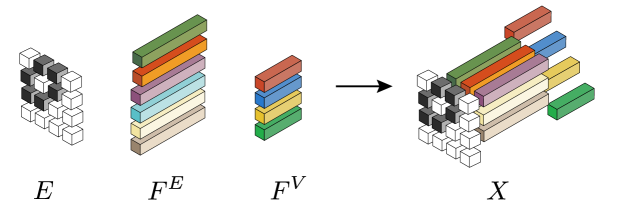
Figure 10: Representing graphs as tensors.

6.1 Equivariant Graph Networks

This section shows how graph neural networks can be deduced from the first principles, namely invariance and equivariance to the action of node permutation. We show how these networks, called Equivariant Graph Networks (EGN), naturally relate to message-passing GNNs and the Weisfeiler–Leman hierarchy and discuss their expressive power.

Representing Graphs as Tensors

We start by setting up some notation. As before, a graph $G$ is denoted $(V,E)$, with node set $V(G)$ and edge set $E(G)$. We let $n=|V(G)|$ and $m=|E(G)|$ denote the number of nodes and edges, respectively. We further assume that the graph has node features $F^{V}$ in $\mathbb{R}^{n\times d}$ and (potentially) edge features $F^{E}$ in $\mathbb{R}^{m\times d}$. In this section, we encode all the graph data, i.e., adjacency information $E(G)$ and features $F^{V}$, and $F^{E}$ as three-dimensional tensors,

$$X\in\mathbb{R}^{n^{2}\times(2d+1)}.$$

The first $n^{2}=n\times n$ slice, namely $X_{:,:,1}$, holds the adjacency matrix of the graph, which is determined by the set of edges $E(G)$. The next $d$ channels $X_{:,:,2:d+1}$ hold the edge features, namely, $X_{i,j,2:d+1}=F^{E}_{e,:}$, where, with a slight abuse of notation, $e=(i,j)$ in $E$. Similarly the last $d$ channels $X_{:,:,d+2:2d+1}$ hold the node features on the diagonal, $X_{i,i,d+2:2d+1}=F^{V}_{i,i,:}$, and zeros on the off-diagonals. See Figure 10 for an illustration of this construction.

A generalization of the graph tensor representation is

$$X\in\mathbb{R}^{n^{k}\times c},$$

where we attach feature vectors in $\mathbb{R}^{c}$ to $k$-tuples of nodes. That is, for a $k$-tuple of nodes $\mathbf{v}=(i_{1},i_{2},\ldots,i_{k})$, for $i_{j}$ in $[n]$, we attach the feature vector $X_{i_{1},i_{2},\ldots,i_{k},:}$ in $\mathbb{R}^{c}$. This representation can be seen as a method of encoding the coloring of the $k$-OWL algorithm as described in Section 3.1, where colors are represented as feature vectors. Furthermore, this representation can be used to represent hypergraphs (Maron et al., 2019b).

An alternative way of representing graphs as tensors is using incidence matrices as suggested in Albooyeh et al. (2019). Here a (feature-less) graph is represented as a tensor $X$ in $\mathbb{R}^{n\times m}$, where $X_{i,e}=1$ if the $i$-th node is incident to the edge $e$, and $X_{i,e}=0$ otherwise. Features on nodes or edges can be encoded using extra channels of $X$. Node features $F^{V}$ can be added as $d$ layers $X_{i,e,2:d+1}=F^{V}_{i,:}$, for all $e$ in $E$, while edge features $X_{i,e,d+2:2d+1}=F^{E}_{e,:}$ for all $i$.

Symmetries of Graph Tensor Representations

Structured objects can often undergo transformations that do not change their essence. Such transformations are called symmetries and are mathematically defined by a group $\mathcal{G}$ that acts on the objects. A well-known example of a symmetry is the translation of an image. Applying a translation to an image does not change the objects appearing in it, assuming they are not taken out of the image boundaries by the translation. Symmetries in graphs arise because the nodes, in most cases, do not follow a canonical order, and any order of the nodes may result in an equivalent yet, seemingly different representation of the graph. More formally, let $S_{n}$ denote the group of permutations on $n$ symbols and a graph represented as a tensor $X$ in $\mathbb{R}^{n\times n\times d}$, as defined above. Then for any $\tau$ in $S_{n}$ a reordered version of the tensor, $\tau\cdot X$, defined by

$$(\tau\cdot X)_{ijk}=X_{\tau^{-1}(i),\tau^{-1}(j),k},$$

represents exactly the same graph. When considering a higher-order tensor representation, the symmetries are defined similarly by $(\tau\cdot X)_{i_{1},\ldots,i_{k},j}=X_{\tau^{-1}(i_{1}),\ldots,\tau^{-1}(i_{k}),j}$.

The incidence tensor representation admits a different symmetry where rows corresponding to nodes and columns corresponding to edges can be permuted independently. That is, for $(\tau,\nu)$ in $S_{n}\times S_{n}$ the symmetry transformation on an incidence matrix $X$ in $\mathbb{R}^{n\times m}$ can be written by $((\tau,\nu)\cdot X)_{ijk}=X_{\tau^{-1}(i),\nu^{-1}(j),k}$; see Albooyeh et al. (2019). In this manuscript, we will focus on the tensor representation and its generalization due to its tight connection to the Weisfeiler–Leman algorithm.

Equivariance as a Design Principle for Neural Networks

The vast majority of graph learning tasks belong to one of two groups: invariant or equivariant. In cases where a single output is predicted for the entire graph, e.g., when solving graph classification problems, the output is often invariant under the node relabeling operation described above, namely $f(\tau\cdot X)=f(X)$. In other cases, predicting values for every node, e.g., in node classification problems or every edge of a graph, may be required. In these cases, the task is often equivariant to the relabeling operation, namely $f(\tau\cdot X)=\tau\cdot f(X)$.

In learning invariant or equivariant graph functions, restricting the model by construction to be invariant or equivariant is often preferable to train more powerful models. For example, recent studies demonstrated that invariant models enjoy better generalization (Bietti et al., 2021; Elesedy and Zaidi, 2021; Garg et al., 2020; Liao et al., 2021; Mei et al., 2021; Sokolic et al., 2017) and improved efficiency (Maron et al., 2019a; Zaheer et al., 2017). Indeed, recent years have seen the introduction of equivariance and invariance as a leading design principle for deep learning models for structured data (Bronstein et al., 2021; Cohen and Welling, 2016; Ravanbakhsh et al., 2017; Wood and Shawe-Taylor, 1996).

Invariant and Equivariant Architectures

To practically build equivariant networks, we first need to choose our graph tensor representation, each endowed with its symmetries, as described above. Second, we compose multiple equivariant layers, as follows,

$$f_{\text{equi}}=L_{1}\circ\dots\circ L_{k},$$

where $L_{i}$ are simple “primitive” equivariant functions with tunable parameters. Drawing inspiration from multi-layer perceptrons (MLPs), each $L_{i}$ can be chosen to be an affine equivariant transformation composed with an entrywise non-linearity, such as the ReLU function. Since invariant linear transformations are often rather limited, invariant networks are constructed by composing a single invariant layer, potentially followed by an MLP, to the equivariant architecture,

$$f_{\text{inv}}=L_{\text{inv}}\circ f_{\text{equi}},$$

where $L_{\text{inv}}$ is some simple, potentially tunable, invariant layer. As a consequence of the constructions just described, the problem of constructing equivariant models is reduced to finding simple and powerful primitive invariant, $L_{\text{inv}}$, and equivariant, $L_{i}$, blocks.

The first paper to consider the construction above for graph learning is the pioneering work of Kondor et al. (2018) that suggested a set of linear and non-linear equivariant layers for tensors with $S_{n}$ symmetry. While not characterizing the full spaces of equivariant layers, the authors identified several important instances: tensor product, tensor contraction, and tensor projection. Since then, a core research theme in this field has become the characterization of useful families of equivariant layers. For the incidence matrix representations, Albooyeh et al. (2019) presented the full characterization of affine layers, while the full characterization for the tensor representation was provided in Maron et al. (2019b).

Linear Equivariant Layers for Graphs

We will elaborate on constructing invariant and equivariant linear layers for the graph tensor representation. To keep things focused and concise, we will assume a single feature dimension and no bias; see further information in Maron et al. (2019a).

A general linear transformation $L:\mathbb{R}^{n^{2}}\rightarrow\mathbb{R}^{n^{2}}$ would be equivariant if it satisfies the following system of linear equations

$$L(\tau\cdot X)=\tau\cdot L(X),\quad\forall X\in\mathbb{R}^{n^{2}},\tau\in S_{n}.$$

To characterize the solutions to this system let us represent $L$ as a tensor $L\in\mathbb{R}^{n^{4}}$, and $L(X)_{i,j}=\sum_{kl}L_{i,j,k,l}X_{k,l}$. Now the above equations take the form:

$$\sum_{kl}L_{i,j,\tau(k),\tau(l)}X_{k,l}=\sum_{kl}L_{\tau^{-1}(i),\tau^{-1}(j),k,l}X_{k,l},$$

which holds for all $X$ and $\tau$ in $S_{n}$ if and only if

$$L_{i,j,k,l}=L_{\tau(i),\tau(j),\tau(k),\tau(l)},\quad\forall\tau\in S_{n}.$$

That is, $L$ is equivariant if it is constant on the orbits of the action of $S_{n}$ on $[n]^{4}$. Each orbit is characterized by a unique equality pattern. For example, all indices $(i_{1},i_{2},i_{3},i_{4})\in[n]^{4}$ such that $i_{1}=i_{2}=i_{3}=i_{4}$ or all indices such that $i_{1}=i_{2}\neq{}i_{3}=i_{4}$. A simple counting argument (Maron et al., 2019c) shows that there are exactly $\text{bell}(4)=15$ such equality patterns. Here, $\text{bell}(k)$ is the bell number which counts the number of different partitions of a set of size $k$. Therefore, the space of equivariant linear operators $L\colon\mathbb{R}^{n^{2}}\to\mathbb{R}^{n^{2}}$ is spanned by the set of indicator matrices of the equality patterns,

$$E^{j}\in\mathbb{R}^{n^{2}\times n^{2}},\quad j\in[15].$$

For example, if the $j$-th equality pattern is given by $i_{1}=i_{2}=i_{3}=i_{4}$ then

$$E^{j}_{i_{1},i_{2},i_{3},i_{4}}=\begin{cases}1&\text{if }i_{1}=i_{2}=i_{3}=i_{4}\\ 0&\text{otherwise. }\\ \end{cases}$$

In Ravanbakhsh et al. (2017); Wood and Shawe-Taylor (1996) this principle is discussed in more general terms. Note, however, that for more general group actions and representations, a closed-form solution and characterization of the space of equivariant linear operators, as done above, might be hard to find or calculate. To summarize the above discussion, we have the following characterization (Maron et al., 2019b).

Theorem 3 (Characterization of linear graph equivariant layers)

The space of linear $S_{n}$-equivariant layers $L\colon\mathbb{R}^{n^{2}}\to\mathbb{R}^{n^{2}}$ is $\text{bell}(4)=15$-dimensional, and can be written as

$$L=\sum_{j=1}^{15}w_{j}E^{j},$$

where each $E^{j}$ in $\mathbb{R}^{n^{2}\times n^{2}}$ is an indicator tensor of an equality pattern on $4$ indices. The scalars $w_{j}$ in $\mathbb{R}$ are the learnable parameters of this layer.

Notably, the dimension of the space of equivariant layers is independent of the graph size $n=|V(G)|$. This crucial property allows practitioners to apply these layers to graphs of any size by using the same learned parameters $w_{j}$ and $E_{j}$ matrices of appropriate size for each graph. Similar arguments as above lead also to a generalization of Theorem 3 to equivariant linear operators between higher order tensors $L\colon\mathbb{R}^{n^{k}}\to\mathbb{R}^{n^{\ell}}$:

Theorem 4 (Characterization of linear hyper-graph equivariant layers)

The space of linear $S_{n}$-equivariant layers $L\colon\mathbb{R}^{n^{k}}\to\mathbb{R}^{n^{\ell}}$ is $\text{bell}(k+l)$ dimensional, and can be written as

$$L=\sum_{j=1}^{\text{bell}(k+l)}w_{j}E^{j},$$

where each $E^{j}$ in $\mathbb{R}^{n^{k}\times n^{l}}$ is an indicator tensor of an equality pattern on $k+l$ indices. As before, the scalars $w_{j}$ in $\mathbb{R}$ are the learnable parameters of this layer.

Non-linear Equivariant Layers for Graphs

A natural generalization of the linear equivariant layers is non-linear equivariant layers. While such characterizations exist, e.g., for equivariant set polynomials $\mathbb{R}^{n}\to\mathbb{R}^{n}$; see for example Segol and Lipman (2020), until recently, it was not known for the more general case of equivariant graph polynomials $\mathbb{R}^{n^{k}}\to\mathbb{R}^{n^{l}}$.

A set of quadratic equivariant tensor operations are suggested in Kondor et al. (2018) based on tensor arithmetic. One systematic way to achieve quadratic equivariant tensor operators based on the above characterization of linear equivariant operators is by composing a tensor product $X\otimes X$ defined by

$$(X\otimes X)_{i_{1},\ldots,i_{k},j_{1},\ldots,j_{l}}=X_{i_{1},\ldots,i_{k}}X_{j_{1},\ldots,j_{l}},$$

with a general linear equivariant operator $\mathbb{R}^{n^{k+l}}\to\mathbb{R}^{n^{m}}$ as characterized in Theorem 4.

Among this myriad of quadratic operators, matrix products have been demonstrated, via relation to Weisfeiler–Leman as described below, to be of particular interest (Maron et al., 2019a). Given two matrices $X^{1}$ and $X^{2}$ in $\mathbb{R}^{n^{2}}$,

$$(X^{1}X^{2})_{i_{1},i_{2}}=\sum_{j=1}^{n}X^{1}_{i_{1},j}X^{2}_{j,i_{2}}.$$ (18)

Furthermore, beyond quadratic operators, the following generalization of matrix product also found a tight connection to higher-order Weisfeiler–Leman algorithms (Azizian and Lelarge, 2020; Maron et al., 2019c). Given $X^{1},\ldots,X^{k}$ in $\mathbb{R}^{n^{k}}$, then $\odot_{i=1}^{k}X^{i}$ in $\mathbb{R}^{n^{k}}$ defined by

$$(\odot_{i=1}^{k}X^{i})_{i_{1},\ldots,i_{k}}=\sum_{j=1}^{n}X^{1}_{j,i_{2},\ldots,i_{k}}X^{2}_{i_{1},j,\ldots,i_{k}}\cdots X^{k}_{i_{1},\ldots,i_{k-1},j}.$$ (19)

Very recently, Puny et al. (2023) provided a full characterization of equivariant graph polynomials $P\colon\mathbb{R}^{n^{2}}\to\mathbb{R}^{n^{2}}$. In particular, they presented a basis for the space of equivariant polynomials, where each element, $P_{H}$, corresponds to a specific multi-graph $H$. These polynomial spaces are used to suggest a new hierarchy for studying the expressive power of GNNs called polynomial expressiveness. Lastly, they discuss how to analyze and enhance the polynomial expressiveness of existing GNN models.

6.2 Expressive Power and Weisfeiler–Leman Hierarchy

Here, we analyze the expressive power of the above linear and non-linear equivariant layers in the context of the Weisfeiler–Leman hierarchy.

Separation Power Versus Function Approximation

There are two main notions used to describe the expressive power of GNNs (Chen et al., 2019), graph separation power, and function approximation power.

Graph separation power refers to the ability of a model class to have an instance that provides a different output on a pair of non-isomorphic graphs $G_{1}$ and $G_{2}$. More formally, we say that a parametric model class $\mathcal{C}=\{f(\,\cdot\,;W)\mid W\in\mathbb{R}^{p}\}$, where $W$ denotes the model’s parameters, can separate a set of graphs $\mathcal{G}$ if for every non-isomorphic $G_{1}$ and $G_{2}$ in $\mathcal{G}$ there exist parameters $W$ such that

$$f(G_{1};W)\neq f(G_{2};W).$$

Function approximation, on the other hand, is the ability of a model class to approximate a given invariant or equivariant function on graphs. Again, more formally, given a compact domain of graphs, $K\subset\mathbb{R}^{n^{2}\times(2d+1)}$, we say that a parametric model class $C$ can approximate some set of continuous invariant functions over $K$, $\mathcal{F}\subset C(K)$, if for every $g$ in $\mathcal{F}$ and $\epsilon>0$ there exist parameters $W$ in $\mathbb{R}^{p}$ such that

$$\|f(\cdot;W)-g(\cdot)\|\leq\epsilon,$$

where $\|\cdot\|$ stands for the $L_{\text{inf}}$ norm on functions: $\|g\|=\max_{x\in K}|g(x)|$.

While seemingly different, Chen et al. (2019) proved that these two notions are equivalent. A model class can separate all graphs if and only if it can approximate any continuous invariant function. We shall later see that Azizian and Lelarge (2020) provided a generalization of this result for $k$-FWL and $k$-OWL separation.

To quantify the power of equivariant graph networks, we would like to measure its separation power compared to the Weisfeiler–Leman hierarchy.

Equivariant Networks With Linear Layers

We now draw the connection between EGNs with linear equivariant layers to the $k$-OWL algorithm. We will show that EGNs can simulate the $k$-OWL algorithm and, consequently, that they have a separation power of at least the $k$-OWL.

To show that, we need to fix a way to represent colors and multisets of colors. Colors will be represented as vectors in some Euclidean space $\mathbb{R}^{d}$. We will need the following lemma for representing multisets of colors.

Lemma 5

Let $\mathbb{R}^{d}$ be a color space, there exist continuous invariant functions $\phi_{j}\colon\mathbb{R}^{d}\to\mathbb{R}$, $j$ in $[J]$, where $J=O((m+d)^{d})$, so that a multiset consisting of $n$ elements in $\mathbb{R}^{d}$, namely $\mathcal{X}=\{\!\!\{x_{i}\in\mathbb{R}^{d}\ |\ i\in[n]\}\!\!\}$, is represented uniquely by a vector in $\mathbb{R}^{J}$ defined by

$$\Phi(\mathcal{X})_{j}=\sum_{i=1}^{n}\phi_{j}(x_{i}).$$

This lemma was proved, e.g., in Maron et al. (2019a). The essence is that $\phi_{j}$ is chosen to be a basis of $d$-multivariate polynomials of degree $n$, and the sum of this basis over the different constituents of $\mathcal{X}$ provides a unique (moment-like) representation to each multiset. Another technical tool we require is a standard approximation power result for MLPs (Hornik, 1991; Pinkus, 1999).

Theorem 6

The set of one hidden layer MLPs with a continuous activation $\sigma$, i.e., $\mathcal{M}(\sigma)=\mathrm{span}\{\sigma(w^{T}x+b)\ |\ w\in\mathbb{R}^{n},b\in\mathbb{R}\}$ is dense in $C(\mathbb{R}^{n})$ in the topology of uniform convergence over compact sets if and only if $\sigma$ is not a polynomial.

Let us consider the multisets $\{\!\!\{C(\ldots,i_{\ell-1},j,i_{\ell+1},\ldots)|\ j\in[n]\}\!\!\}$ required for implementing the update rule of the $k$-OWL. Consider the following linear operator $T\colon\mathbb{R}^{n^{k}}\to\mathbb{R}^{n^{k}\times k}$

$$(TX)_{i_{1},\ldots,i_{k},\ell}\mapsto\sum_{j}X_{\ldots,i_{\ell-1},j,i_{\ell+1},\ldots}.$$

This operator is equivariant, as can be verified directly from the definition. In particular, this operator belongs to the linear space characterized in Theorem 4, i.e., there is a choice of $w_{j}$ so that $L=T$. Applying $T$ to each feature dimension after applying $x\mapsto(\phi_{1}(x),\ldots,\phi_{J}(x))$ to each feature vector of $X$, namely $X_{i_{1},\ldots,i_{k},:}$ in $\mathbb{R}^{d}$, encodes the colors. That is, if $Y$ is the output of this operation, then $Y_{i_{1},\ldots,i_{k},:,:}$ uniquely represents the neighborhood $M^{*}(i_{1},\ldots,i_{k})$ of the $k$-OWL algorithm (see Equation 5). Using Theorem 6 to replace the $\phi_{j}$ maps with arbitrary good MLP approximations concludes that $f_{\text{equi}}$ equipped with linear equivariant layers as in Theorem 4 can represent the update step of $k$-OWL. Note, however, that tensors of order $k$ are used in the network. We say $f$ is $k$-order if it uses tensors of degrees less or equal to $k$. Consequently, $k$-order $f_{\text{equi}}$ can represent any finite number of $k$-OWL update steps. This is the core argument in the following theorem (Maron et al., 2019c).

Theorem 7

Given two non-isomorphic graphs $G_{1}$ and $G_{2}$ that can be distinguished by $k$-OWL algorithm, there exists $k$-order $f_{inv}$ and weights $W$ so that $f_{\text{inv}}(G_{1};W)\neq f_{\text{inv}}(G_{2};W)$.

EGNs with Polynomial Layers and $k$-WL

The matrix product, Equation 18, and the generalized matrix product, Equation 19, can be used to design equivariant graph networks that can simulate the $k$-FWL algorithm (Azizian and Lelarge, 2020; Maron et al., 2019c). The connection between matrix products and the $k$-FWL test can be illustrated by considering the case $k=2$ studied in Maron et al. (2019c), where it was shown that second-order EGNs augmented with a matrix product operation are capable of simulating 2-FWL. In order to demonstrate this, the authors exploit the similarity between the 2-FWL’s update rule in Equation (3) and the matrix multiplication from Equation 18. More specifically, when $k=2$, $M_{i}$, which represents the neighbor aggregation in the $2$-FWL update rule, takes the form: $M_{i}(\mathbf{v})=\{(C^{k}_{i}(v,w),C^{k}_{i}(w,v))\mid w\in V(G)\}$. Upon closer inspection, it becomes apparent that this is a set of tuples whose indices have a striking similarity to those used in matrix multiplication. See more details in Maron et al. (2019b). This can be generalized to higher-order $k$-EGNs with the generalized matrix product in Equation (19) and $k$-FWL. We name these architectures FEGN, to emphasize the relation to FWL. Similarly, we call EGNs with linear layers OEGN. A summary of the separation results of FEGN and OEGN is provided by Azizian and Lelarge (2020); Geerts (2020).

Theorem 8

The separation power of $k$-order OEGN coincides with the separation power of $k$-OWL. The separation power of $k$-order FEGN coincides with that of $k$-FWL.

Universality

Several papers have studied the approximation power of EGNs rather than their ability to separate non-isomorphic graphs. Maron et al. (2019b) proved the universality of $G$-invariant networks for any permutation group $G$ when using (very) high-order tensors. When choosing the appropriate permutation group, this also applies to OEGNs. This construction, however, is not feasible as it uses $O(n^{4})$ order tensors. A more efficient, but still unfeasible, construction of universal OEGNs was presented in Ravanbakhsh (2020); another proof can be found in Maehara and NT (2019). Keriven and Peyré (2019); Azizian and Lelarge (2020) expanded these results to equivariant functions.

	$k$-OEGN	$k$-FEGN
Time	$\mathcal{O}(n^{k}\cdot\text{bell}(2k))$	$\mathcal{O}(n^{k+1}\cdot k)$
Space	$\mathcal{O}(n^{k})$	$\mathcal{O}(n^{k})$

Table 1: Time and space complexity of LEGNs and OEGNs with a constant number of layers.

Efficient Implementation

Thus far, we have mainly discussed the theoretical properties of EGNs. The next step is to discuss how these models can be effectively implemented. A straightforward way to implement the linear layer used by OEGNs involves constructing matrices with values defined according to equality patterns on the indices, as described above. The main disadvantages of this construction are (1) it scales poorly and is impractical for large values of $n$, and (2) the basis elements lack intuitive meaning. For the $k=2$ case, an alternative was suggested by Maron et al. (2019b, Appendix A). In particular, the authors proposed forming a new basis for the space of linear equivariant functions, in which each basis element is defined as a sum of several previous basis elements. The summands are carefully chosen so that each new basis element represents a simple operation and can be implemented in $O(n^{2})$ time complexity, without constructing the aforementioned $n^{2}\times n^{2}$ indicator matrix. Here is a partial list of the resulting basis elements: a scaled identity operator for the diagonal or the off-diagonal part of the matrix, a row summation operator that broadcasts the sum to the rows or the columns, and a diagonal summation operator that broadcasts the sum to the diagonal or the off-diagonal. A complete list can be found in Maron et al. (2019b). Albooyeh et al. (2019) generalized this idea by showing that for general $k$, all linear equivariant layers can be written as a composition of linear pooling (summation) and broadcasting operators. A lesser amount of thought was given to implementing the generalized matrix multiplication from Equation (19). To our knowledge, only the case $k=2$ was implemented by standard matrix multiplication (Maron et al., 2019a; Chen et al., 2019; Azizian and Lelarge, 2020). Time and space complexity: Table 1 summarizes the space and time complexity of OEGNs, employing the layers from Theorem 4, and FEGNs, using the layers from Equation (19), with a constant number of layers and feature dimensions.

The (local) $k$-OWL-based architectures proposed in Morris et al. (2020b) are implemented quite differently. Each graph with $n$ nodes simulates the $k$-OWL on an auxiliary graph $G^{\otimes k}$ on $n^{k}$ vertices defined as follows. The vertex set of $G^{\otimes k}$ is the set $V(G)^{k}$ of all $k$-tuples in $V(G)^{k}$. The edge set of $G^{\otimes k}$ is defined as follows. Two $k$-tuples $s$ and $t$ are connected by an edge in $G^{\otimes k}$ if they are local $i$-neighbors for $i$ in $[k]$; see Section 4.5. Such edge is annotated with the label $i$. On top of the auxiliary graph $G^{\otimes k}$, they use a GNN powerful enough to simulate a variant of the $1$-WL taking edge labels into account. Morris et al. (2019) used a similar strategy for the set-based version of Equation 16.

7 Expressivity and Generalization Abilities of GNNs

The previous sections show that GNNs’ expressive power is reasonably well understood by exploiting their connection to the Weisfeiler–Leman hierarchy. While there exists works upper bounding GNNs’ generalization error, e.g., Garg et al. (2020); Liao et al. (2021); Scarselli et al. (2018), these approaches express GNNs’ generalization ability using only classical graph parameters, e.g., maximum degree, number of vertices, or edges, which cannot fully capture the complex structure of real-world graphs. Recently, Morris et al. (2023) made progress connecting GNNs’ expressive power and generalization ability via the Weisfeiler–Leman hierarchy. They studied the influence of graph structure and the parameters’ encoding lengths on GNNs’ generalization by tightly connecting $1$-WL’s expressivity and GNNs’ Vapnik–Chervonenkis (VC) dimension (Vapnik, 1995). They derived that GNNs’ VC dimension depends tightly on the number of equivalence classes computed by the $1$-WL over a given set of graphs. Moreover, the results easily extend to the $k$-WL and many recent, more expressive GNN extensions. Moreover, they showed that GNNs’ VC dimension depends logarithmically on the number of colors computed by the $1$-WL and polynomially on the number of parameters.

8 Applications

Structured data is ubiquitous in many disciplines, such as cheminformatics, bioinformatics, neuroscience, natural language processing, social network analysis, and computer vision. The considered data can typically be represented as graphs, but the modeling is not necessarily unique. For example, in bioinformatics, the nodes of a protein graph may represent the amino acids or the secondary structure elements formed by sequences of amino acids. Likewise, the nodes and edges may be annotated by additional information in the form of attributes. In general, the used graph model can significantly influence learning methods for graphs. For the comparison of machine learning methods, several standard benchmark data sets were introduced (Hu et al., 2020; Morris et al., 2020a), which contain graphs representing various objects and concepts such as small molecules, proteins, and protein-protein interactions, citation networks, as well as letters, fingerprints, and cuneiform signs. The considered tasks include node, edge, and graph classification or regression in supervised, semi-supervised, and unsupervised settings. General-purpose graph learning methods based on or closely related to the Weisfeiler–Leman method are applied in all these domains and settings and have proven to be highly effective (Kriege et al., 2020; Morris et al., 2020a).

In the following, we review the development in selected application areas and focus on domain-specific constraints, for which Weisfeiler–Leman type algorithms have been adapted. Moreover, we present applications of the Weisfeiler–Leman method in a broader context of machine learning.

8.1 Computer Programs

The Weisfeiler–Leman graph kernel was used to determine the similarity of computer programs (Li et al., 2016). To this end, either the API calls made by the program or the data flow between procedures is represented by a graph. The nodes are labeled by the procedure’s name and the data type, respectively. Using this graph model, the similarity computed by the Weisfeiler–Leman graph kernel can, for example, help to find related source code on internet repositories for reuse.

Narayanan et al. (2016) observed that for malware detection, an extended graph model is required. To distinguish regular from malicious code, additional context information is essential, e.g., whether a user is aware or unaware of the execution of the code. This context information was added to the graph model, and the Weisfeiler–Leman graph kernel was adapted to incorporate the additional context labels in the re-labeling procedure.

8.2 Semantic Web

Knowledge graphs are a prime example of heterogeneous graphs, in which nodes and edges have different types. For example, nodes may be of type “person” or type “movie,” each having a different set of attributes. Further, an edge between a person and a movie can, among others, represent an “is-actor-in” or “is-screenwriter-of” relationship. De Vries (2013) modified the Weisfeiler–Leman graph kernel for application to general Resource Description Framework (RDF) data. RDF data consists of subject-predicate-object statements. These form directed multigraphs with node and edge labels when interpreted as edges. Typically, one is interested in the similarity between subgraphs extracted for specific instances. Instead of applying the Weisfeiler–Leman graph kernel to such subgraphs, the Weisfeiler–Leman labels are computed in the whole graph but are distinguished according to their depth regarding instances of interest. By this means, the computation was accelerated compared to the subgraph-based method.

8.3 Cheminformatics

As detailed in Section 1.2.2, methods that encode the neighborhoods of atoms have been developed in cheminformatics independently of the Weisfeiler–Leman method and were widely used for analyzing molecular data before the Weisfeiler–Leman graph kernel was introduced. Besides parallel developments, research in machine learning with graphs and cheminformatics strongly influenced each other. Since the development of neural networks for graphs gained momentum in machine learning, new methods were quickly adapted for cheminformatics tasks (Wieder et al., 2020).

In the standard graph representation of molecules, the atoms correspond to nodes and chemical bonds to edges. A particularity in cheminformatics is that the properties of interest typically depend on the conformations of molecules, i.e., the geometrical arrangement of the atoms in a 3-dimensional space. Since a molecule can have different conformations, determining the relevant one is often part of the problem. However, this information should be exploited for successful learning when reliable coordinates are available. Gilmer et al. (2017) applied GNNs to predict quantum properties and represented 3-dimensional coordinates by adding edges encoding the inter-atom distances to obtain rotation-invariance. Klicpera et al. (2020) adapted the message-passing approach of GNNs by incorporating the direction in coordinate space to model angular potentials.

For the prediction of fuel ignition quality, Schweidtmann et al. (2020) proposed a graph neural network architecture relying on standard molecular graphs annotated with atomic and bond features. The proposed GNN model uses a recurrent neural network architecture with a hierarchical combination of standard and higher-order GNNs to capture the long-range effects of atom groups within a molecule. The method shows competitive performance compared to state-of-the-art domain-specific models.

Apart from the standard graph representation of molecules, further models exist, typically representing groups of connected atoms such as rings by a single node with additional attributes (Rarey and Dixon, 1998; Stiefl et al., 2006). Fey et al. (2020b) proposed a hierarchical architecture where two GNNs run simultaneously on two graph representations at different levels of abstraction, passing messages inside each graph and exchanging messages between the two representations. The combination of a standard molecular graph model with an adaption of a tree-like representation (Rarey and Dixon, 1998) is shown to increase the expressivity of the GNN architecture (Fey et al., 2020b).

8.4 Computer Vision and Graphics

Graphs have also been becoming increasingly popular in the computer vision domain for learning on scene graphs (Raposo et al., 2017; Xu et al., 2017), image keypoints (Li et al., 2019; Fey et al., 2020a; Kriege et al., 2018a), superpixels (Monti et al., 2017), 3D point clouds (Qi et al., 2017) and manifolds (Fey et al., 2018; Hanocka et al., 2019) where relational learning introduces a critical inductive bias into the model. Notably, various new GNN variants have been proposed, derived as differentiable versions of the $1$-WL algorithm that can incorporate continuous spatial and semantic information into the neighborhood aggregation phase. However, only a few works make this connection explicit.

For example, Zaheer et al. (2017) proposed the popular DeepSets model, e.g., for learning on point clouds, and were the first who studied universality guarantees for fixed-size, countable sets and uncountable sets of invariant deep neural network architectures, pioneering work for the connection of $1$-WL and GNNs. Herzig et al. (2018) extends this study and characterizes all permutation invariant architectures applied to predicting scene graphs from images. Furthermore, Fey et al. (2020a) tackles the task of keypoint matching in natural images by using a differentiable validator for graph isomorphism based on the $1$-WL heuristic; see also the next section.

8.5 Graph Matching

A common principle in comparing graphs is identifying correspondences between their nodes that optimally preserve the edge structure. The problem arises in various domains, and variations have been studied under different terms such as maximum common subgraph isomorphism (Kriege et al., 2017), network alignment (Zhang and Tong, 2016), graph matching (Gold and Rangarajan, 1996) or graph edit distance (Sanfeliu and Fu, 1983), often using different algorithmic approaches. These problems are NP-hard, and heuristics are widely applied in practice. A particular simple and efficient approach (Kriege et al., 2019) applies Weisfeiler–Leman refinement to both graphs to obtain a hierarchy as shown in Figure 7. Then, the nodes of the first graph are assigned to the nodes of the second graph by traversing the hierarchy from the leaves to the root. At each node in the hierarchy, all available nodes are matched, and the remaining nodes are passed to the parent in the hierarchy for matching in a later step. By performing the matching within the color classes using the structural results of Arvind et al. (2015), it can be guaranteed that the approach constructs an isomorphism for two isomorphic graphs that are amenable to Weisfeiler–Leman refinement (Arvind et al., 2015; Kriege et al., 2019). Moreover, the node correspondences obtained by this approach preserve more structural information, i.e., lead to a smaller graph edit distance, on several real-world data sets than comparable heuristics that are computationally more demanding (Kriege et al., 2019). Stöcker et al. (2019) showed that for graphs representing protein complexes, a similarity measure defined with Weisfeiler–Leman labels highly correlates with the graph edit similarity obtained from a minimal sequence of edit operations.

Recent work by Bai et al. (2019, 2020) suggests learning similarities or distances based on graph matching using graph neural networks. The graph edit distance has been approximated using shared GNNs, where the output is fine-tuned by a (non-differentiable) histogram of correspondence scores (Bai et al., 2019). In follow-up work, Bai et al. (2020) proposed to order the correspondence matrix in a breadth-first-search fashion and to process it further with the help of traditional CNNs. The approaches are affected by the limited expressivity of the used GNNs and do not provide approximation guarantees. Qin et al. (2020) proposed to learn embeddings for graphs using GNNs reflecting the graph edit distance for similarity search in databases using semantic hashing.

Another recent direction, referred to as deep graph matching, uses pairwise node similarities obtained from the node features learned by GNNs (Fey et al., 2020a; Wang et al., 2019; Zanfir and Sminchisescu, 2018). Fey et al. (2020a) proposed a method to iteratively improve the consistency of the similarities in a subsequent second stage via a differentiable validator for graph isomorphism based on the $1$-WL heuristic. The approach maps node identifiers of one graph according to the current node similarities and distributes them via GNNs synchronously in both graphs. The node similarities are then optimized to reduce the resulting node features’ differences. The optimization step resembles classical gradient-based graph matching heuristics, which solve a sequence of linear assignment problems (Gold and Rangarajan, 1996). Among other domains, this method significantly improves the alignment of cross-lingual knowledge bases (Fey et al., 2020a).

9 Open Challenges, Limitations, Future Research Directions

The present work shows that the Weisfeiler–Leman algorithm, its connection to GNNs, and more powerful equivariant architectures for graphs have led to many meaningful insights, advancing machine learning with graphs and relational structures. However, there remain several open challenges in this area of research, some of which we outline here, along with limitations and directions for future work.

9.1 Understanding the Interplay of Expressive Power, Generalization, and Optimization

Although the results presented here, especially the results of Section 6.2, neatly characterize the expressive power of equivariant neural architecture based on the Weisfeiler–Leman method, these universal architectures suffer from an exponential dependence on $k$, e.g., due to operating on $k$-order tensors, making them infeasible for large-scale graphs, resulting in the following challenge.

Open Challenge 1

Design provably powerful equivariant neural architectures for graphs that better control the trade-off between expressive power and scalability.

Moreover, the expressivity results are of an existentialist nature. While they show the existence of an architecture’s weight assignment, they do not guarantee that standard first-order optimization methods, e.g., Kingma and Ba (2015), converge to them. Hence, it is an open challenge to understand the interplay of expressive power and optimization.

Open Challenge 2

Understand how first-order optimization methods impact the expressive power of WL-based equivariant architecture for graphs.

Even more, the relationship between generalization and optimization is understood to a lesser extent. Although some results are shedding some light on the generalization ability using classical tools from learning theory, see, e.g., Garg et al. (2020); Kriege et al. (2018b); Liao et al. (2021); Xu et al. (2020), there exists little research in understanding how optimization influences generalization and what impact graph structure plays. To the best of our knowledge, only Xu et al. (2021) tackle this problem, relying on a linearized GNN architecture, and investigate the effect of skip connections, depth, or good label distribution on the convergence during training. Hence, to further investigate this problem, we propose the following open challenge.

Open Challenge 3

Understand how first-order optimization methods impact the generalization abilities of WL-based equivariant architectures for graphs.

9.2 Locality and the Role of Depth

The number of iterations of the $1$-WL or layers of a GNN architecture is typically selected by cross-validation and often small, e.g., smaller than $5$. For larger values, 1-WL’s features become too specific, leading to overfitting for graph kernels. In contrast, under particular assumptions, the GNNs’ node features become indistinguishable, a phenomenon referred to as over-smoothing (Liu et al., 2020). Moreover, for GNNs, the bottleneck problem refers to the observation that large neighborhoods cannot be accurately represented (Alon and Yahav, 2020). These problems prevent both methods from capturing global or long-range information. Contrarily, depth, i.e., the number of layers, seems to play a crucial role in the loss landscape of (general) neural networks, e.g., Poggio et al. (2019), resulting in the following challenge.

Open Challenge 4

Understand the impact of depth in WL-based equivariant architectures on expressivity, optimization, and generalization, and design architectures that can provably capture long-range dependency.

9.3 Incorporating Expert Knowledge

Nowadays, kernels based on the $1$-WL and GNNs are heavily used in life sciences to engineering applications. However, their usage is often ad-hoc, not leveraging crucial expert knowledge. In cheminformatics, for example, information on functional groups or pharmacophore properties is often available, but it is not straightforward to explicitly incorporate it into the $1$-WL and GNN pipeline. Hence, we view the development of mechanisms to include such knowledge as a crucial step in making WL-based learning with graphs more applicable to real-world domains, resulting in the following challenge.

Open Challenge 5

Derive a methodology to incorporate expert knowledge, i.e., designing WL-based equivariant architectures that provably capture task-relevant graph structure specified by domain experts.

9.4 Limitations and Future Research Directions

While the Weisfeiler–Leman algorithm’s connections lead to a better understanding of GNNs, it also has limitations. Since the Weisfeiler–Leman algorithm is purely discrete, it is unclear what it reveals about GNNs’ expressivity in the presence of attributed graphs, i.e., nodes annotated with a real-valued vector. For example, the presence of additional (real-valued) attributes, which $1$-WL cannot process adequately, might lead to GNNs distinguishing pairs of nodes that the Weisfeiler–Leman algorithm cannot distinguish. Hence, understanding how to adapt the Weisfeiler–Leman paradigm to this setting remains an open challenge. Moreover, the Weisfeiler–Leman hierarchy might be a too coarse-grained yardstick to understand GNNs’ expressivity. For example, in the case of trees already, $1$-WL does not give any insights since it solves the isomorphism problem for trees.

Further, even for more complex graph classes, the algorithm only reveals if a GNN will distinguish non-isomorphic graphs within that class. However, it does not indicate if structurally similar graphs will be mapped to features that are close concerning some distance. Hence, developing a more fine-grained hierarchy might lead to new insights. Finally, the algorithm only captures the expressivity of GNNs following the message-passing framework, see Equation 15, not of the multitude of spectral GNNs. Hence, understanding how spectral information can enhance or complement the Weisfeiler–Leman algorithm and GNNs is vital, resulting in the following challenge.

Open Challenge 6

Understand how the Weisfeiler–Leman algorithm can be used to define a more fine-grained notion of similarity beyond the binary graph isomorphism objective.

10 Conclusion

We have provided an overview of the uses of the Weisfeiler–Leman method for machine learning with graphs. To this end, we introduced the $1$-WL and its more powerful generalization, the $k$-dimensional Weisfeiler–Leman algorithm, and outlined its theoretical properties. We then thoroughly surveyed graph kernels based on the Weisfeiler–Leman method. Subsequently, we presented results connecting the $1$-WL and graph neural networks, followed by an overview of neural architecture surpassing the limits of the former. Moreover, we gave an in-depth overview of provably powerful equivariant architectures on graphs and their connection to the $k$-WL and surveyed applications for WL-based machine learning architectures. Finally, we identified open challenges in the field and provided directions for future research.

We hope our survey presents a helpful handbook of graph representation learning methods, perspectives, and limitations and that its insights and principles will help spur novel research results at the intersection of graph theory and machine learning.

References

- Aamand et al. (2022) A. Aamand, J. Y. Chen, P. Indyk, S. Narayanan, R. Rubinfeld, N. Schiefer, S. Silwal, and T. Wagner. Exponentially improving the complexity of simulating the Weisfeiler-Lehman test with graph neural networks. In Advances in Neural Information Processing Systems, 2022.
- Abboud et al. (2021) R. Abboud, İ. İ. Ceylan, M. Grohe, and T. Lukasiewicz. The surprising power of graph neural networks with random node initialization. In International Joint Conference on Artificial Intelligence, pages 2112–2118, 2021.
- Adamson and Bush (1973) G. W. Adamson and J. A. Bush. A method for the automatic classification of chemical structures. Information Storage and Retrieval, 9(10):561 – 568, 1973.
- Albooyeh et al. (2019) M. Albooyeh, D. Bertolini, and S. Ravanbakhsh. Incidence networks for geometric deep learning. CoRR, abs/1905.11460, 2019.
- Alon and Yahav (2020) U. Alon and E. Yahav. On the bottleneck of graph neural networks and its practical implications. CoRR, abs/2006.05205, 2020.
- Arvind et al. (2015) V. Arvind, J. Köbler, G. Rattan, and O. Verbitsky. On the power of color refinement. In International Symposium on Fundamentals of Computation Theory, pages 339–350, 2015.
- Athreya et al. (2017) A. Athreya, D. E. Fishkind, M. Tang, C. E. Priebe, Y. Park, J. T. Vogelstein, K. D. Levin, V. Lyzinski, Y. Qin, and D. L. Sussman. Statistical inference on random dot product graphs: a survey. Journal of Machine Learning Research, 18:226:1–226:92, 2017.
- Atserias and Maneva (2013) A. Atserias and E. N. Maneva. Sherali-adams relaxations and indistinguishability in counting logics. SIAM Journal on Computing, 42(1):112–137, 2013.
- Atserias and Ochremiak (2018) A. Atserias and J. Ochremiak. Definable ellipsoid method, sums-of-squares proofs, and the isomorphism problem. In ACM/IEEE Symposium on Logic in Computer Science, pages 66–75, 2018.
- Atserias et al. (2019) A. Atserias, L. Mancinska, D. E. Roberson, R. Sámal, S. Severini, and A. Varvitsiotis. Quantum and non-signalling graph isomorphisms. Journal of Combinatorial Theory, Series B, 136:289–328, 2019.
- Azizian and Lelarge (2020) W. Azizian and M. Lelarge. Characterizing the expressive power of invariant and equivariant graph neural networks. CoRR, abs/2006.15646, 2020.
- Babai (1979) L. Babai. Lectures on graph isomorphism. University of Toronto, Department of Computer Science. Mimeographed lecture notes, October 1979, 1979.
- Babai (2016) L. Babai. Graph isomorphism in quasipolynomial time. In ACM Symposium on Theory of Computing, pages 684–697, 2016.
- Babai and Kucera (1979) L. Babai and L. Kucera. Canonical labelling of graphs in linear average time. In Symposium on Foundations of Computer Science, pages 39–46, 1979.
- Babai et al. (1980) L. Babai, P. Erdős, and S. M. Selkow. Random graph isomorphism. SIAM Journal on Computing, 9(3):628–635, 1980.
- Bai et al. (2019) Y. Bai, H. Ding, S. Bian, T. Chen, Y. Sun, and W. Wang. SimGNN: A neural network approach to fast graph similarity computation. In ACM International Conference on Web Search and Data Mining, pages 384–392, 2019.
- Bai et al. (2020) Y. Bai, H. Ding, K. Gu, Y. Sun, and W. Wang. Learning-based efficient graph similarity computation via multi-scale convolutional set matching. In AAAI Conference on Artificial Intelligence, pages 3219–3226, 2020.
- Balcilar et al. (2021) M. Balcilar, P. Héroux, B. Gaüzère, P. Vasseur, S. Adam, and P. Honeine. Breaking the limits of message passing graph neural networks. In International Conference on Machine Learning, pages 599–608, 2021.
- Barabasi and Oltvai (2004) A.-L. Barabasi and Z. N. Oltvai. Network biology: Understanding the cell’s functional organization. Nature Reviews Genetics, 5(2):101–113, 2004.
- Barceló et al. (2020) P. Barceló, E. V. Kostylev, M. Monet, J. Pérez, J. L. Reutter, and J. P. Silva. The logical expressiveness of graph neural networks. In International Conference on Learning Representations, 2020.
- Barceló et al. (2021) P. Barceló, F. Geerts, J. L. Reutter, and M. Ryschkov. Graph neural networks with local graph parameters. CoRR, abs/2106.06707, 2021.
- Baskin et al. (1997) I. I. Baskin, V. A. Palyulin, and N. S. Zefirov. A neural device for searching direct correlations between structures and properties of chemical compounds. Journal of Chemical Information and Computer Sciences, 37(4):715–721, 1997.
- Beaini et al. (2020) D. Beaini, S. Passaro, V. Létourneau, W. L. Hamilton, G. Corso, and P. Liò. Directional graph networks. CoRR, abs/2010.02863, 2020.
- Bender et al. (2004) A. Bender, H. Y. Mussa, R. C. Glen, and S. Reiling. Molecular similarity searching using atom environments, information-based feature selection, and a naïve bayesian classifier. Journal of Chemical Information and Modeling, 44(1):170–178, 2004.
- Berkholz and Grohe (2015) C. Berkholz and M. Grohe. Limitations of algebraic approaches to graph isomorphism testing. In International Colloquium on Automata, Languages, and Programming, pages 155–166, 2015.
- Berkholz and Grohe (2017) C. Berkholz and M. Grohe. Linear diophantine equations, group csps, and graph isomorphism. In ACM/SIAM Symposium on Discrete Algorithms, pages 327–339, 2017.
- Berkholz et al. (2017) C. Berkholz, P. S. Bonsma, and M. Grohe. Tight lower and upper bounds for the complexity of canonical colour refinement. Theory of Computing Systems, 60(4):581–614, 2017.
- Bevilacqua et al. (2021) B. Bevilacqua, F. Frasca, D. Lim, B. Srinivasan, C. Cai, G. Balamurugan, M. M. Bronstein, and H. Maron. Equivariant subgraph aggregation networks. CoRR, abs/2110.02910, 2021.
- Bietti et al. (2021) A. Bietti, L. Venturi, and J. Bruna. On the sample complexity of learning under geometric stability. In Advances in Neural Information Processing Systems, pages 18673–18684, 2021.
- Biggs et al. (1986) N. L. Biggs, E. K. Lloyd, and R. J. Wilson. Graph Theory 1736-1936. Clarendon Press, 1986.
- Bodnar et al. (2021a) C. Bodnar, F. Frasca, N. Otter, Y. G. Wang, P. Liò, G. Montúfar, and M. M. Bronstein. Weisfeiler and Lehman go cellular: CW networks. In Advances in Neural Information Processing Systems, 2021a.
- Bodnar et al. (2021b) C. Bodnar, F. Frasca, Y. Wang, N. Otter, G. F. Montufar, P. Lió, and M. Bronstein. Weisfeiler and Lehman go topological: Message passing simplicial networks. In International Conference on Machine Learning, pages 1026–1037, 2021b.
- Bollobás (1982) B. Bollobás. Distinguishing vertices of random graphs. Annals of Discrete Mathematics, 13:33–50, 1982.
- Bollobás (2002) B. Bollobás. Modern Graph Theory. Springer, 2002.
- Bondy (1991) J. A. Bondy. A graph reconstructor’s manual. Surveys in combinatorics, 166:221–252, 1991.
- Borgwardt and Kriegel (2005) K. M. Borgwardt and H.-P. Kriegel. Shortest-path kernels on graphs. In IEEE International Conference on Data Mining, pages 74–81, 2005.
- Borgwardt et al. (2005) K. M. Borgwardt, C. S. Ong, S. Schönauer, S. V. N. Vishwanathan, A. J. Smola, and H.-P. Kriegel. Protein function prediction via graph kernels. Bioinformatics, 21(Supplement 1):i47–i56, 2005.
- Borgwardt et al. (2020) K. M. Borgwardt, M. E. Ghisu, F. Llinares-López, L. O’Bray, and B. Rieck. Graph kernels: State-of-the-art and future challenges. Foundations and Trends in Machine Learning, 13(5-6), 2020.
- Bouritsas et al. (2023) G. Bouritsas, F. Frasca, S. Zafeiriou, and M. M. Bronstein. Improving graph neural network expressivity via subgraph isomorphism counting. IEEE Transactions on Pattern Analysis and Machine Intelligence, 45(1):657–668, 2023.
- Bronstein et al. (2021) M. M. Bronstein, J. Bruna, T. Cohen, and P. Velickovic. Geometric deep learning: Grids, groups, graphs, geodesics, and gauges. CoRR, abs/2104.13478, 2021.
- Bruna et al. (2014) J. Bruna, W. Zaremba, A. Szlam, and Y. LeCun. Spectral networks and deep locally connected networks on graphs. In International Conference on Learning Representation, 2014.
- Cai et al. (1992) J. Cai, M. Fürer, and N. Immerman. An optimal lower bound on the number of variables for graph identifications. Combinatorica, 12(4):389–410, 1992.
- Cardon and Crochemore (1982) A. Cardon and M. Crochemore. Partitioning a graph in . Theoretical Computer Science, 19(1):85 – 98, 1982.
- Chami et al. (2020) I. Chami, S. Abu-El-Haija, B. Perozzi, C. Ré, and K. Murphy. Machine learning on graphs: A model and comprehensive taxonomy. CoRR, abs/2005.03675, 2020.
- Chang et al. (2008) K.-W. Chang, C.-J. Hsieh, and C.-J. Lin. Coordinate descent method for large-scale l2-loss linear support vector machines. Journal of Machine Learning Research, 9:1369–1398, 2008.
- Chen et al. (2019) Z. Chen, S. Villar, L. Chen, and J. Bruna. On the equivalence between graph isomorphism testing and function approximation with GNNs. In Advances in Neural Information Processing Systems, pages 15868–15876, 2019.
- Cohen and Welling (2016) T. Cohen and M. Welling. Group equivariant convolutional networks. In International Conference on Machine Learning, pages 2990–2999, 2016.
- Costa and De Grave (2010) F. Costa and K. De Grave. Fast neighborhood subgraph pairwise distance kernel. In International Conference on Machine Learning, pages 255–262, 2010.
- Cotta et al. (2021) L. Cotta, C. Morris, and B. Ribeiro. Reconstruction for powerful graph representations. In Advances in Neural Information Processing Systems, pages 1713–1726, 2021.
- Czajka and Pandurangan (2008) T. Czajka and G. Pandurangan. Improved random graph isomorphism. Journal of Discrete Algorithms, 6(1):85–92, 2008.
- Dasoulas et al. (2020) G. Dasoulas, L. D. Santos, K. Scaman, and A. Virmaux. Coloring graph neural networks for node disambiguation. In International Joint Conference on Artificial Intelligence, pages 2126–2132, 2020.
- Datar et al. (2004) M. Datar, N. Immorlica, P. Indyk, and V. S. Mirrokni. Locality-sensitive hashing scheme based on -stable distributions. In ACM Symposium on Computational Geometry, pages 253–262, 2004.
- Daylight (2008) Daylight. Chemical information systems daylight, daylight theory manual v4.9. http://www.daylight.com/dayhtml/doc/theory, 2008. URL http://www.daylight.com/dayhtml/doc/theory.
- Defferrard et al. (2016) M. Defferrard, B. X., and P. Vandergheynst. Convolutional neural networks on graphs with fast localized spectral filtering. In Advances in Neural Information Processing Systems, pages 3844–3852, 2016.
- Dell et al. (2018) H. Dell, M. Grohe, and G. Rattan. Lovász meets Weisfeiler and Leman. In International Colloquium on Automata, Languages, and Programming, pages 40:1–40:14, 2018.
- Dubois (1973) J. E. Dubois. French national policy for chemical information and the DARC system as a potential tool of this policy. Journal of Chemical Documentation, 13(1):8–13, 1973.
- Dubois et al. (1987) J. E. Dubois, A. Panaye, and R. Attias. DARC system: notions of defined and generic substructures. filiation and coding of FREL substructure (SS) classes. Journal of Chemical Information and Computer Sciences, 27(2):74–82, 1987.
- Durant et al. (2002) J. L. Durant, B. A. L., D. R. Henry, and J. G. Nourse. Reoptimization of MDL keys for use in drug discovery. Journal of Chemical Information and Computer Sciences, 42(5):1273–1280, 2002.
- Duvenaud et al. (2015) D. K. Duvenaud, D. Maclaurin, J. Iparraguirre, R. Bombarell, T. Hirzel, A. Aspuru-Guzik, and R. P. Adams. Convolutional networks on graphs for learning molecular fingerprints. In Advances in Neural Information Processing Systems, pages 2224–2232, 2015.
- Dvorák (2010) Z. Dvorák. On recognizing graphs by numbers of homomorphisms. Journal of Graph Theory, 64(4):330–342, 2010.
- Easley and Kleinberg (2010) D. Easley and J. Kleinberg. Networks, Crowds, and Markets: Reasoning About a Highly Connected World. Cambridge University Press, 2010.
- Elesedy and Zaidi (2021) B. Elesedy and S. Zaidi. Provably strict generalisation benefit for equivariant models. In International Conference on Machine Learning, pages 2959–2969, 2021.
- Evdokimov et al. (2000) S. Evdokimov, I. N. Ponomarenko, and G. Tinhofer. Forestal algebras and algebraic forests (on a new class of weakly compact graphs). Discrete Mathematics, 225(1-3):149–172, 2000.
- Fey et al. (2018) M. Fey, J. E. Lenssen, F. Weichert, and H. Müller. SplineCNN: Fast geometric deep learning with continuous B-spline kernels. In IEEE Conference on Computer Vision and Pattern Recognition, pages 869–877, 2018.
- Fey et al. (2020a) M. Fey, J. E. Lenssen, C. Morris, J. Masci, and N. M. Kriege. Deep graph matching consensus. In International Conference on Learning Representations, 2020a.
- Fey et al. (2020b) M. Fey, J. Yuen, and F. Weichert. Hierarchical inter-message passing for learning on molecular graphs. CoRR, abs/2006.12179, 2020b.
- Figueras (1993) J. Figueras. Morgan revisited. Journal of Chemical Information and Computer Sciences, 33(5):717–718, 1993.
- Frasca et al. (2022) F. Frasca, B. Bevilacqua, M. M. Bronstein, and H. Maron. Understanding and extending subgraph GNNs by rethinking their symmetries. CoRR, abs/2206.11140, 2022.
- Fröhlich et al. (2005) H. Fröhlich, J. K. Wegner, F. Sieker, and A. Zell. Optimal assignment kernels for attributed molecular graphs. In ACM International Conference on Machine Learning, pages 225–232, 2005.
- Fürer (2001) M. Fürer. Weisfeiler-Lehman refinement requires at least a linear number of iterations. In International Colloquium on Automata, Languages and Programming, pages 322–333, 2001.
- Gama et al. (2019) F. Gama, A. G. Marques, G. Leus, and A. Ribeiro. Convolutional neural network architectures for signals supported on graphs. IEEE Trans. Signal Process., 67(4):1034–1049, 2019.
- Garg et al. (2020) V. Garg, S. Jegelka, and T. Jaakkola. Generalization and representational limits of graph neural networks. In International Conference on Machine Learning, pages 3419–3430, 2020.
- Gärtner et al. (2003) T. Gärtner, P. Flach, and S. Wrobel. On graph kernels: Hardness results and efficient alternatives. In Learning Theory and Kernel Machines, pages 129–143. Springer, 2003.
- Geerts (2020) F. Geerts. The expressive power of kth-order invariant graph networks. CoRR, abs/2007.12035, 2020.
- Geerts et al. (2020) F. Geerts, F. Mazowiecki, and G. A. Pérez. Let’s agree to degree: Comparing graph convolutional networks in the message-passing framework. CoRR, abs/2004.02593, 2020.
- Gilmer et al. (2017) J. Gilmer, S. S. Schoenholz, P. F. Riley, O. Vinyals, and G. E. Dahl. Neural message passing for quantum chemistry. In International Conference on Machine Learning, 2017.
- Gold and Rangarajan (1996) S. Gold and A. Rangarajan. A graduated assignment algorithm for graph matching. IEEE Transaction on Pattern Analysis and Machine Intelligence, 18(4):377–388, 1996.
- Grädel et al. (2019) E. Grädel, M. Grohe, B. Pago, and W. Pakusa. A finite-model-theoretic view on propositional proof complexity. Logical Methods in Computer Science, 15(1), 2019.
- Grohe (1999) M. Grohe. Equivalence in finite-variable logics is complete for polynomial time. Combinatorica, 19(4):507–532, 1999.
- Grohe (2000) M. Grohe. Isomorphism testing for embeddable graphs through definability. In ACM Symposium on Theory of Computing, pages 63–72, 2000.
- Grohe (2012) M. Grohe. Fixed-point definability and polynomial time on graphs with excluded minors. Journal of the ACM, 59(5):27:1–27:64, 2012.
- Grohe (2017) M. Grohe. Descriptive Complexity, Canonisation, and Graph Structure Theory. Cambridge University Press, 2017.
- Grohe (2021) M. Grohe. The logic of graph neural networks. In ACM/IEEE Symposium on Logic in Computer Science, pages 1–17, 2021.
- Grohe and Kiefer (2021) M. Grohe and S. Kiefer. Logarithmic Weisfeiler-Leman identifies all planar graphs. In International Colloquium on Automata, Languages, and Programming, volume 198, pages 134:1–134:20, 2021.
- Grohe and Neuen (2019) M. Grohe and D. Neuen. Canonisation and definability for graphs of bounded rank width. In ACM/IEEE Symposium on Logic in Computer Science, pages 1–13, 2019.
- Grohe and Neuen (2021) M. Grohe and D. Neuen. Recent advances on the graph isomorphism problem. In Survey in Combinatorics, volume 470, pages 187–234. Cambridge University Press, 2021.
- Grohe and Otto (2015) M. Grohe and M. Otto. Pebble games and linear equations. Journal of Symbolic Logic, 80(3):797–844, 2015. doi: 10.1017/jsl.2015.28.
- Grohe et al. (2014) M. Grohe, K. Kersting, M. Mladenov, and E. Selman. Dimension reduction via colour refinement. In European Symposium on Algorithms, pages 505–516, 2014.
- Haasdonk and Bahlmann (2004) B. Haasdonk and C. Bahlmann. Learning with distance substitution kernels. In Pattern Recognition, pages 220–227. Elsevier, 2004.
- Hamilton et al. (2017) W. L. Hamilton, R. Ying, and J. Leskovec. Inductive representation learning on large graphs. In Advances in Neural Information Processing Systems, pages 1025–1035, 2017.
- Hanocka et al. (2019) R. Hanocka, A. Hertz, N. Fish, R. Giryes, S. Fleishman, and D. Cohen-Or. Meshcnn: A network with an edge. ACM Transactions on Graphics, 38(4):90, 2019.
- Haussler (1999) D. Haussler. Convolution kernels on discrete structures. Technical Report UCS-CRL-99-10, University of California at Santa Cruz, 1999.
- Hensel et al. (2021) F. Hensel, M. Moor, and B. Rieck. A survey of topological machine learning methods. Frontiers in Artificial Intelligence, 4, 2021.
- Herzig et al. (2018) R. Herzig, M. Raboh, G. Chechik, J. Berant, and A. Globerson. Mapping images to scene graphs with permutation-invariant structured prediction. In Advances in Neural Information Processing Systems, 2018.
- Horn et al. (2022) M. Horn, E. De Brouwer, M. Moor, Y. Moreau, B. Rieck, and K. Borgwardt. Topological graph neural networks. In International Conference on Learning Representations, 2022.
- Hornik (1991) K. Hornik. Approximation capabilities of multilayer feedforward networks. Neural networks, 4(2):251–257, 1991.
- Horváth et al. (2010) T. Horváth, J. Ramon, and S. Wrobel. Frequent subgraph mining in outerplanar graphs. Data Mining and Knowledge Discovery, 21:472–508, 2010.
- Hu et al. (2020) W. Hu, M. Fey, M. Zitnik, Y. Dong, H. Ren, B. Liu, M. Catasta, and J. Leskovec. Open graph benchmark: Datasets for machine learning on graphs. In Advances in Neural Information Processing Systems, 2020.
- Hu et al. (2022) Y. Hu, X. Wang, Z. Lin, P. Li, and M. Zhang. Two-dimensional Weisfeiler-Lehman graph neural networks for link prediction. CoRR, abs/2206.09567, 2022.
- Immerman and Lander (1990) N. Immerman and E. Lander. Describing Graphs: A First-Order Approach to Graph Canonization, pages 59–81. Springer, 1990.
- Johansson and Dubhashi (2015) F. D. Johansson and D. Dubhashi. Learning with similarity functions on graphs using matchings of geometric embeddings. In ACM Conference on Knowledge Discovery and Data Mining, pages 467–476, 2015.
- Jumper et al. (2021) J. Jumper, R. Evans, A. Pritzel, T. Green, M. Figurnov, O. Ronneberger, K. Tunyasuvunakool, R. Bates, A. Žídek, A. Potapenko, A. Bridgland, C. Meyer, S. A. A. Kohl, A. J. Ballard, A. Cowie, B. Romera-Paredes, S. Nikolov, R. Jain, J. Adler, T. Back, S. Petersen, D. Reiman, E. Clancy, M. Zielinski, M. Steinegger, M. Pacholska, T. Berghammer, S. Bodenstein, D. Silver, O. Vinyals, A. W. Senior, K. Kavukcuoglu, P. Kohli, and D. Hassabis. Highly accurate protein structure prediction with AlphaFold. Nature, 2021.
- Kang et al. (2012) U. Kang, H. Tong, and J. Sun. Fast random walk graph kernel. In SIAM International Conference on Data Mining, pages 828–838, 2012.
- Karp (1979) R. M. Karp. Probabilistic analysis of a canonical numbering algorithm for graphs. Proceedings of Symposia in Pure Mathematics, 34:365–378, 1979.
- Kashima et al. (2003) H. Kashima, K. Tsuda, and A. Inokuchi. Marginalized kernels between labeled graphs. In International Conference on Machine Learning, pages 321–328, 2003.
- Keriven and Peyré (2019) N. Keriven and G. Peyré. Universal invariant and equivariant graph neural networks. In Advances in Neural Information Processing Systems, pages 7090–7099, 2019.
- Keriven et al. (2021) N. Keriven, A. Bietti, and S. Vaiter. On the universality of graph neural networks on large random graphs. In Advances in Neural Information Processing Systems, pages 6960–6971, 2021.
- Kersting et al. (2014) K. Kersting, M. Mladenov, R. Garnett, and M. Grohe. Power iterated color refinement. In AAAI Conference on Artificial Intelligence, pages 1904–1910, 2014.
- Kiefer (2020a) S. Kiefer. Power and Limits of the Weisfeiler-Leman Algorithm. PhD thesis, Department of Computer Science, RWTH Aachen University, 2020a.
- Kiefer (2020b) S. Kiefer. The Weisfeiler-Leman algorithm: an exploration of its power. ACM SIGLOG News, 7(3):5–27, 2020b.
- Kiefer and McKay (2020) S. Kiefer and B. D. McKay. The iteration number of colour refinement. In International Colloquium on Automata, Languages, and Programming, pages 73:1–73:19, 2020.
- Kiefer and Schweitzer (2016) S. Kiefer and P. Schweitzer. Upper bounds on the quantifier depth for graph differentiation in first order logic. In ACM/IEEE Symposium on Logic in Computer Science, pages 287–296, 2016.
- Kiefer et al. (2015) S. Kiefer, P. Schweitzer, and E. Selman. Graphs identified by logics with counting. In International Symposium on Mathematical Foundations of Computer Science, pages 319–330, 2015.
- Kiefer et al. (2019) S. Kiefer, I. Ponomarenko, and P. Schweitzer. The weisfeiler-leman dimension of planar graphs is at most 3. Journal of the ACM, 66(6):44:1–44:31, 2019.
- Kim et al. (2022) J. Kim, T. D. Nguyen, S. Min, S. Cho, M. Lee, H. Lee, and S. Hong. Pure transformers are powerful graph learners. CoRR, 2022.
- Kingma and Ba (2015) D. P. Kingma and J. Ba. Adam: A method for stochastic optimization. In International Conference on Learning Representations, 2015.
- Kipf and Welling (2017) T. N. Kipf and M. Welling. Semi-supervised classification with graph convolutional networks. In International Conference on Learning Representations, 2017.
- Kireev (1995) D. B. Kireev. Chemnet: A novel neural network based method for graph/property mapping. Journal of Chemical Information and Computer Sciences, 35(2):175–180, 1995.
- Klicpera et al. (2020) J. Klicpera, J. Groß, and S. Günnemann. Directional message passing for molecular graphs. In International Conference on Learning Representations, 2020.
- Kondor and Pan (2016) R. Kondor and H. Pan. The multiscale laplacian graph kernel. In Advances in Neural Information Processing Systems, pages 2982–2990, 2016.
- Kondor et al. (2018) R. Kondor, H. T. Son, H. Pan, B. M. Anderson, and S. Trivedi. Covariant compositional networks for learning graphs. In International Conference on Learning Representations, 2018.
- Kriege and Mutzel (2012) N. Kriege and P. Mutzel. Subgraph matching kernels for attributed graphs. In International Conference on Machine Learning. Omnipress, 2012.
- Kriege et al. (2017) N. Kriege, F. Kurpicz, and P. Mutzel. On maximum common subgraph problems in series-parallel graphs. European Journal on Combinatorics, 2017.
- Kriege (2019) N. M. Kriege. Deep Weisfeiler-Lehman assignment kernels via multiple kernel learning. In European Symposium on Artificial Neural Networks, 2019.
- Kriege (2022) N. M. Kriege. Weisfeiler and Leman go walking: Random walk kernels revisited. In Advances in Neural Information Processing Systems, pages 20119–20132, 2022.
- Kriege et al. (2016) N. M. Kriege, G. P.-L., and R. C. Wilson. On valid optimal assignment kernels and applications to graph classification. In Advances in Neural Information Processing Systems, pages 1615–1623, 2016.
- Kriege et al. (2018a) N. M. Kriege, M. Fey, D. Fisseler, P. Mutzel, and F. Weichert. Recognizing cuneiform signs using graph based methods. In Workshop on Cost-Sensitive Learning, pages 31–44, 5 2018a.
- Kriege et al. (2018b) N. M. Kriege, C. Morris, A. Rey, and C. Sohler. A property testing framework for the theoretical expressivity of graph kernels. In International Joint Conference on Artificial Intelligence, pages 2348–2354, 2018b.
- Kriege et al. (2019) N. M. Kriege, P.-L. Giscard, F. Bause, and R. C. Wilson. Computing optimal assignments in linear time for approximate graph matching. In IEEE International Conference on Data Mining, pages 349–358, 2019.
- Kriege et al. (2020) N. M. Kriege, F. D. Johansson, and C. Morris. A survey on graph kernels. Applied Network Science, 5(1):6, 2020.
- LeCun et al. (2015) Y. LeCun, Y. Bengio, and G. Hinton. Deep learning. Nature, 521(7553):436–444, 2015.
- Levie et al. (2019) R. Levie, F. Monti, X. Bresson, and M. M. Bronstein. Cayleynets: Graph convolutional neural networks with complex rational spectral filters. IEEE Trans. Signal Process., 67(1):97–109, 2019.
- Li et al. (2020) P. Li, Y. Wang, H. Wang, and J. Leskovec. Distance encoding: Design provably more powerful neural networks for graph representation learning. In Advances in Neural Information Processing Systems, 2020.
- Li et al. (2016) W. Li, H. Saidi, H. Sanchez, M. Schäf, and P. Schweitzer. Detecting similar programs via the Weisfeiler-Leman graph kernel. In International Conference on Software Reuse, pages 315–330, 2016.
- Li et al. (2019) Y. Li, C. Gu, T. Dullien, O. Vinyals, and P. Kohli. Graph matching networks for learning the similarity of graph structured objects. In International Conference on Machine Learning, pages 3835–3845, 2019.
- Liao et al. (2021) R. Liao, R. Urtasun, and R. Zemel. A PAC-bayesian approach to generalization bounds for graph neural networks. In International Conference on Learning Representations, 2021.
- Lichter et al. (2019) M. Lichter, I. Ponomarenko, and P. Schweitzer. Walk refinement, walk logic, and the iteration number of the Weisfeiler-Leman algorithm. In ACM/IEEE Symposium on Logic in Computer Science, pages 1–13, 2019.
- Lipton (1978) R. J. Lipton. The beacon set approach to graph isomorphism. Technical report, Yale University, 1978.
- Liu et al. (2020) M. Liu, H. Gao, and S. Ji. Towards deeper graph neural networks. In ACM Conference on Knowledge Discovery and Data Mining, pages 338–348, 2020.
- Loosli et al. (2016) G. Loosli, S. Canu, and C. S. Ong. Learning SVM in Kreĭn spaces. IEEE Transactions on Pattern Analysis and Machine Intelligence, 38(6):1204–1216, 2016.
- Maehara and NT (2019) T. Maehara and H. NT. A simple proof of the universality of invariant/equivariant graph neural networks. CoRR, abs/1910.03802, 2019.
- Malkin (2014) P. N. Malkin. Sherali–Adams relaxations of graph isomorphism polytopes. Discrete Optimization, 12:73–97, 2014.
- Maron et al. (2019a) H. Maron, H. Ben-Hamu, H. Serviansky, and Y. Lipman. Provably powerful graph networks. CoRR, abs/1905.11136, 2019a.
- Maron et al. (2019b) H. Maron, H. Ben-Hamu, N. Shamir, and Y. Lipman. Invariant and equivariant graph networks. In International Conference on Learning Representations, 2019b.
- Maron et al. (2019c) H. Maron, E. Fetaya, N. Segol, and Y. Lipman. On the universality of invariant networks. In International Conference on Machine Learning, pages 4363–4371, 2019c.
- Maron et al. (2020) H. Maron, O. Litany, G. Chechik, and E. Fetaya. On learning sets of symmetric elements. In International Conference on Machine Learning, pages 6734–6744, 2020.
- McKay (1981) B. McKay. Practical graph isomorphism. Congressus Numerantium, 30:45–87, 1981.
- Mei et al. (2021) S. Mei, T. Misiakiewicz, and A. Montanari. Learning with invariances in random features and kernel models. In Conference on Learning Theory, pages 3351–3418, 2021.
- Merkwirth and Lengauer (2005) C. Merkwirth and T. Lengauer. Automatic generation of complementary descriptors with molecular graph networks. Journal of Chemical Information and Modeling, 45(5):1159–1168, 2005.
- Micheli (2009) A. Micheli. Neural network for graphs: A contextual constructive approach. IEEE Transactions on Neural Networks, 20(3):498–511, 2009.
- Micheli and Sestito (2005) A. Micheli and A. S. Sestito. A new neural network model for contextual processing of graphs. In Italian Workshop on Neural Nets Neural Nets and International Workshop on Natural and Artificial Immune Systems, pages 10–17, 2005.
- Milo et al. (2002) R. Milo, S. Shen-Orr, S. Itzkovitz, N. Kashtan, D. Chklovskii, and U. Alon. Network motifs: simple building blocks of complex networks. Science, 298(5594):824–827, 2002.
- Mohri et al. (2012) M. Mohri, A. Rostamizadeh, and A. Talwalkar. Foundations of Machine Learning. MIT Press, 2012.
- Monti et al. (2017) F. Monti, D. Boscaini, J. Masci, E. Rodolà, J. Svoboda, and M. M. Bronstein. Geometric deep learning on graphs and manifolds using mixture model CNNs. In IEEE Conference on Computer Vision and Pattern Recognition, pages 5425–5434, 2017.
- Morgan (1965) H. L. Morgan. The generation of a unique machine description for chemical structures-a technique developed at chemical abstracts service. Journal of Chemical Documentation, 5(2):107–113, 1965.
- Morris et al. (2016) C. Morris, N. M. Kriege, K. Kersting, and P. Mutzel. Faster kernel for graphs with continuous attributes via hashing. In IEEE International Conference on Data Mining, pages 1095–1100, 2016.
- Morris et al. (2017) C. Morris, K. Kersting, and P. Mutzel. Glocalized Weisfeiler-Lehman kernels: Global-local feature maps of graphs. In IEEE International Conference on Data Mining, pages 327–336, 2017.
- Morris et al. (2019) C. Morris, M. Ritzert, M. Fey, W. L. Hamilton, J. E. Lenssen, G. Rattan, and M. Grohe. Weisfeiler and leman go neural: Higher-order graph neural networks. In AAAI Conference on Artificial Intelligence, pages 4602–4609, 2019.
- Morris et al. (2020a) C. Morris, N. M. Kriege, F. Bause, K. Kersting, P. Mutzel, and M. Neumann. TUDataset: A collection of benchmark datasets for learning with graphs. CoRR, abs/2007.08663, 2020a.
- Morris et al. (2020b) C. Morris, G. Rattan, and P. Mutzel. Weisfeiler and Leman go sparse: Towards higher-order graph embeddings. In Advances in Neural Information Processing Systems, 2020b.
- Morris et al. (2022) C. Morris, G. Rattan, S. Kiefer, and S. Ravanbakhsh. SpeqNets: Sparsity-aware permutation-equivariant graph networks. In International Conference on Machine Learning, pages 16017–16042, 2022.
- Morris et al. (2023) C. Morris, F. Geerts, J. Tönshoff, and M. Grohe. WL meet VC. CoRR, abs/2301.11039, 2023.
- Müller et al. (2023) L. Müller, M. Galkin, C. Morris, and L. Rampásek. Attending to graph transformers. CoRR, abs/2302.04181, 2023.
- Murphy et al. (2019a) R. L. Murphy, B. Srinivasan, V. A. Rao, and B. Ribeiro. Janossy pooling: Learning deep permutation-invariant functions for variable-size inputs. In International Conference on Learning Representations, 2019a.
- Murphy et al. (2019b) R. L. Murphy, B. Srinivasan, V. A. Rao, and B. Ribeiro. Relational pooling for graph representations. In International Conference on Machine Learning, pages 4663–4673, 2019b.
- Narayanan et al. (2016) A. Narayanan, G. Meng, L. Yang, J. Liu, and L. Chen. Contextual weisfeiler-lehman graph kernel for malware detection. In International Joint Conference on Neural Networks, pages 4701–4708, 2016.
- Newman (2003) M. E. J. Newman. The structure and function of complex networks. SIAM review, 45(2):167–256, 2003.
- Niepert et al. (2021) M. Niepert, P. Minervini, and L. Franceschi. Implicit MLE: backpropagating through discrete exponential family distributions. Advances in Neural Information Processing Systems, 34:14567–14579, 2021.
- Nikolentzos et al. (2017) G. Nikolentzos, P. Meladianos, and M. Vazirgiannis. Matching node embeddings for graph similarity. In AAAI Conference on Artificial Intelligence, pages 2429–2435, 2017.
- NT and Maehara (2020) H. NT and T. Maehara. Graph homomorphism convolution. CoRR, abs/2005.01214, 2020.
- O’Donnell et al. (2014) R. O’Donnell, J. Wright, C. Wu, and Y. Zhou. Hardness of robust graph isomorphism, Lasserre gaps, and asymmetry of random graphs. In ACM/SIAM Symposium on Discrete Algorithms, pages 1659–1677, 2014.
- Orsini et al. (2015) F. Orsini, P. Frasconi, and L. De Raedt. Graph invariant kernels. In International Joint Conference on Artificial Intelligence, pages 3756–3762, 2015.
- Otto (1997) M. Otto. Bounded variable logics and counting – A study in finite models, volume 9 of Lecture Notes in Logic. Springer, 1997.
- Paige and Tarjan (1987) R. Paige and R. Tarjan. Three partition refinement algorithms. SIAM Journal on Computing, 16(6):973–989, 1987.
- Papp and Wattenhofer (2022) P. A. Papp and R. Wattenhofer. A theoretical comparison of graph neural network extensions. In International Conference on Machine Learning, pages 17323–17345, 2022.
- Papp et al. (2021) P. A. Papp, K. Martinkus, L. Faber, and R. Wattenhofer. Dropgnn: Random dropouts increase the expressiveness of graph neural networks. In Advances in Neural Information Processing Systems, 2021.
- Pinkus (1999) A. Pinkus. Approximation theory of the MLP model in neural networks. Acta numerica, 8:143–195, 1999.
- Poggio et al. (2019) T. A. Poggio, A. Banburski, and Q. Liao. Theoretical issues in deep networks: Approximation, optimization and generalization. CoRR, abs/1908.09375, 2019.
- Puny et al. (2020) O. Puny, H. Ben-Hamu, and Y. Lipman. From graph low-rank global attention to 2-FWL approximation. CoRR, abs/2006.07846, 2020.
- Puny et al. (2023) O. Puny, D. Lim, B. T. Kiani, H. Maron, and Y. Lipman. Equivariant polynomials for graph neural networks. CoRR, abs/2302.11556, 2023.
- Qi et al. (2017) C. R. Qi, , H. Su, K. Mo, and L. J. Guibas. PointNet: Deep learning on point sets for 3D classification and segmentation. In IEEE Conference on Computer Vision and Pattern Recognition, pages 77–85, 2017.
- Qian et al. (2022) C. Qian, G. Rattan, F. Geerts, C. Morris, and M. Niepert. Ordered subgraph aggregation networks. CoRR, abs/2206.11168, 2022.
- Qin et al. (2020) Z. Qin, Y. Bai, and Y. Sun. Ghashing: Semantic graph hashing for approximate similarity search in graph databases. In ACM Conference on Knowledge Discovery and Data Mining, pages 2062–2072, 2020.
- Ralaivola et al. (2005) L. Ralaivola, S. J. Swamidass, H. Saigo, and P. Baldi. Graph kernels for chemical informatics. Neural Networks, 18(8):1093–1110, 2005.
- Ramakrishnan et al. (2014) R. Ramakrishnan, O. Dral, P., M. Rupp, and O. A. von Lilienfeld. Quantum chemistry structures and properties of 134 kilo molecules. Scientific Data, 1, 2014. Nature.
- Raposo et al. (2017) D. Raposo, A. Santoro, D. G. T. Barrett, R. Pascanu, T. Lillicrap, and P. W. Battaglia. Discovering objects and their relations from entangled scene representations. In International Conference on Learning Representations, 2017.
- Rarey and Dixon (1998) M. Rarey and J. S. Dixon. Feature trees: A new molecular similarity measure based on tree matching. Journal of Computer-Aided Molecular Design, 12:471–490, 1998.
- Ravanbakhsh (2020) S. Ravanbakhsh. Universal equivariant multilayer perceptrons. In International Conference on Machine Learning, pages 7996–8006, 2020.
- Ravanbakhsh et al. (2017) S. Ravanbakhsh, J. Schneider, and B. Poczos. Equivariance through parameter-sharing. In International Conference on Machine Learning, pages 2892–2901, 2017.
- Razinger (1982) M. Razinger. Extended connectivity in chemical graphs. Theoretica chimica acta, 61(6):581–586, 1982.
- Rieck (2023) B. Rieck. On the expressivity of persistent homology in graph learning. CoRR, abs/2302.09826, 2023.
- Rieck et al. (2019) B. Rieck, C. Bock, and K. M. Borgwardt. A persistent Weisfeiler-Lehman procedure for graph classification. In International Conference on Machine Learning, pages 5448–5458, 2019.
- Robertson et al. (1993) N. Robertson, P. Seymour, and R. Thomas. Linkless embeddings of graphs in 3-space. Bulletin of the AMS, 28:84–89, 1993.
- Rogers and Hahn (2010) D. Rogers and M. Hahn. Extended-connectivity fingerprints. Journal of Chemical Information and Modeling, 50(5):742–754, May 2010.
- Sandfelder et al. (2021) D. Sandfelder, P. Vijayan, and W. L. Hamilton. Ego-GNNs: Exploiting ego structures in graph neural networks. In IEEE International Conference on Acoustics, Speech and Signal Processing, pages 8523–8527, 2021.
- Sanfeliu and Fu (1983) A. Sanfeliu and K.-S. Fu. A distance measure between attributed relational graphs for pattern recognition. IEEE Transactions on Systems, Man, and Cybernetics, 13(3):353–362, 1983.
- Sato et al. (2020) R. Sato, M. Yamada, and H. Kashima. Random features strengthen graph neural networks. CoRR, abs/2002.03155, 2020.
- Scarselli et al. (2009) F. Scarselli, M. Gori, A. C. Tsoi, M. Hagenbuchner, and G. Monfardini. The graph neural network model. IEEE Transactions on Neural Networks, 20(1):61–80, 2009.
- Scarselli et al. (2018) F. Scarselli, A. C. Tsoi, and M. Hagenbuchner. The Vapnik-Chervonenkis dimension of graph and recursive neural networks. Neural Networks, pages 248–259, 2018.
- Schweidtmann et al. (2020) A. M. Schweidtmann, J. G. Rittig, A. König, M. Grohe, A. Mitsos, and M. Dahmen. Graph neural networks for prediction of fuel ignition quality. Energy & Fuels, 34(9):11395–11407, 2020.
- Segol and Lipman (2020) N. Segol and Y. Lipman. On universal equivariant set networks. In International Conference on Learning Representations, 2020.
- Shalev-Shwartz and Ben-David (2014) S. Shalev-Shwartz and S. Ben-David. Understanding Machine Learning: From Theory to Algorithms. Cambridge University Press, 2014.