Stability analysis of the Hindmarsh-Rose neuron under electromagnetic induction

Abstract

We consider the Hindmarsh-Rose neuron model modified by taking into account the effect of electromagnetic induction on membrane potential. We study the impact of the magnetic flux on the neuron dynamics, through the analysis of the stability of fixed points. Increasing magnetic flux reduces the number of equilibrium points and favors their stability. Therefore, electromagnetic induction tends to regularize chaotic regimes and to affect regular and quasi-regular ones by reducing the number of spikes or even destroying the oscillations.

Keywords: Hindmarsh–Rose neuron with electromagnetic induction, linear stability analysis, bifurcation diagrams.

I Introduction

The functioning of the fundamental cell of the nervous system (the neuron) has been the subject of research in various scientific fields. Beyond the fundamental questions of neuroscience, advances in understanding the mechanisms of neuronal activities and their responses to external stimuli can be helpful, for instance, in the development of artificial intelligence and other technologies. So, many efforts have been made to grasp, through model systems, the dynamics of real biological neurons. Among the successful mathematical models, consistent with experimental observations, let us mention those of Hodgkin-Huxley hodgkin52 ; hasegawa00 ; kang15 , Morris-Lecar morris81 ; hu16 ; shi14 , Izhikevich izhikevich03 , FitzHugh-Nagumo kosmidis03 ; abbasian13 ; wang07 and Hindmarsh-Rose (HR) HR82 ; HR84 ; innocenti07 ; wu16 , to name just a few. These models can be improved by incorporating specific features. For instance in neural circuits, the introduction of piezoeletric  auditory2021 or light-sensitive elements light2021 is currently under investigation to mimic auditory or visual responses.

Another important feature that gained attention more recently is the influence of induced magnetic fields. Electrophysiological activity can induce magnetic fluxes due to time-varying currents, which can affect the membrane potential. Moreover, although electrical and chemical synapses have a crucial role in the transmission of information between neurons, the exchange of signals can also occur through the flow of ionic currents through gap junctions that allow direct passage between cells, a mechanism that can be affected by the influence of electromagnetic fields. The effect of electromagnetic induction has been taken into account introducing modifications in the above mentioned neuronal models. This has typically been done via memory resistance (memristor) coupling of the magnetic flux to membrane potential bao10 ; muthuswamy10 ; li15 , in Fitzhugh-Nagumo wuwang16 , Hodgkin-Huxley wuwang17 ; xu18 and HR lv16 ; wuxu17 ; parastesh18 ; usha19 neurons. The inclusion of memristive effects has been shown crucial, for instance, to explain effects in heart tissues due to electromagnetic radiation wuwang16 . Networks of coupled neurons, under magnetic flow, have also been investigated parastesh18 ; parastesh19 ; mostaghimi19 ; alternating , identifying diverse spatiotemporal patterns including wave propagation and chimera states. The later are particularly interesting since are intermediate between order and disorder and have been observed in diverse neural networks lakshmanan2019 ; makarov2021 .

In this work we focus on the single neuron dynamics with the inclusion of memristive effects. We consider an extended version of the HR neuronal model, previously proposed to take into account the adjustment of the membrane potential due to a magnetic flux across it lv16 . This model has been investigated before, mainly for oscillatory external current lv16 or external field parastesh18 , or both wuxu17 . Here we study the dynamical regimes that arise when changing the strength of the induction coupling, under constant external inputs. The type of regime is relevant since it can determine the neuro-computational capacity of the cells to process the inputs and communicate the output to other cells morris81 ; houart99 ; izhikevich00 .

The paper is structured as follows. In Section II, we summarize the MHR model and define the values of the parameters. In Section  III, we present the results from the stability analysis and bifurcation diagrams. Section IV, we highlight the main findings.

II Neuronal model of Hindmarsh-Rose with electromagnetic induction

The HR model of neuronal bursting has been proposed in Ref. HR84 and thereafter has been intensively studied and extended in several directions houart99 ; innocenti07 ; yamapi13 ; wang13 ; hilda16 ; wu16 ; rajagopal19 . In its original version, it consists of the following set of three coupled first-order nonlinear differential equations:

$$\left\{\begin{array}[]{ll}\dot{x}=y-ax^{3}+bx^{2}-z+I_{ext},\\ \dot{y}=c-dx^{2}-y,\\ \dot{z}=r[s(x-x_{0})-z],\end{array}\right.$$ (1)

where the variables $x$, $y$ and $z$ describe the membrane potential, the recovery and adaptation ionic currents, respectively, with $I_{ext}$ denoting the external forcing current, and $a$, $b$, $c$, $d$, $r$, $s$ and $x_{0}$ are typically positive constants. As expected for biological neuron models, it takes into account the membrane potential as well as the currents through ion channels that regulate ion propagation. However, neuronal activity depends on complex external and internal influences. In particular, the effect of the magnetic flux $\phi$ across the cell membrane can affect its potential via a memristor effect. Then, to describe the interaction between neuronal activity and a magnetic flux, a fourth dimension was added to Eq. (1), and the resulting four-dimensional neuron model, modified HR (MHR) lv16 ; usha19 , is expressed as

$$\left\{\begin{array}[]{ll}\dot{x}=y-ax^{3}+bx^{2}-z+I_{ext}-kxM(\phi),\\ \dot{y}=c-dx^{2}-y,\\ \dot{z}=r[s(x-x_{0})-z],\\ \dot{\phi}=k_{1}x-k_{2}\phi,\end{array}\right.$$ (2)

where $M(\phi)$ represents the coupling between the magnetic flux across the membrane, $\Phi$, and the membrane potential $x$. The term $-kM(\Phi)x$ denotes the current produced through electromagnetic induction, modulated by the intensity $k$. This current, together with the external current $I_{ext}$, contributes to the change in the membrane potential (see Ref. lv16 for further details). $M(\phi)$ is assumed equivalent to the memductance of a magnetic flux-controlled memristor li15 ; lv16 , modelled by $M(\phi)=\alpha+3\beta\phi^{2}$ lv16 ; usha19 , where $\alpha$ and $\beta$ are positive parameters. This quadratic form represents a minimal nonlinear model, smooth, positive definite, increasing with the flux intensity. Let us mention that discontinuous (piece-wise linear) forms have been also studied in the literature of the modified HR neuron parastesh18 . Finally, the parameters $k_{1}$ and $k_{2}$ are rates that control the evolution of the magnetic flux, governed by the membrane potential and leakage.

Let us remark that other extensions of the HR neuron have been considered before, for instance with variable signals lv16 ; wuxu17 in the MHR, or modification of the equation of the recovery current in the HR hilda16 ; rajagopal19 , differently to the MHR model here considered, in which the equation for the potential is adjusted.

In the numerical simulations, we will use the physiologically relevant values $a=1$, $b=3$, $c=1$, $d=5$, as in the standard HR84 and extended lv16 HR models. The threshold potential was set $x_{0}=-1.6$, and we will typically set $r=0.001$ and $s=4$, unless other values are specified. For the memory function, we set $\alpha=0.1$ and $\beta=0.06$, and the coefficients that rule the magnetic flux dynamics are $k_{1}=0.1$, $k_{2}=0.5$ yamapi13 .

The constant external excitation current $I_{ext}$ and the strength $k$ of the magnetic term are the main control parameters, which will be varied throughout this work. In stability analyses, we will also vary the adaptation parameters $r$ and $s$.

III Analysis of the dynamics of the MHR model

III.1 Equilibrium points

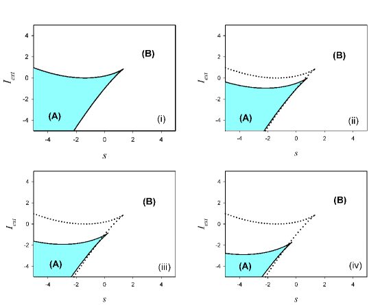
Figure 1: Regions characterized by the number of equilibrium points in the $s-I_{ext}$ plane, for different values of the magnetic-flux coupling parameter: $k=0$ (i), $k=5$ (ii), $k=10$ (iii) and $k=15$ (iv). In the shadowed region (A) there are three equilibrium points, while in region (B), there is a single equilibrium point. At the border (full lines), there are two equilibrium points. The dotted line repeats the case $k=0$, for comparison. Notice that the region (A) shrinks with increasing $k$.

The fixed points of the system of equations presented in Eq. (2) are obtained by setting the time derivatives equal to zero, which leads to a systems of nonlinear algebraic equations whose solution gives equilibrium points of the form parastesh18

$$E=(x_{e},y_{e},z_{e},\phi_{e})=(x_{e},-dx_{e}^{2}+c,s(x_{e}-x_{0}),k_{1}x_{e}/k_{2}),$$ (3)

where the equilibrium potential $x_{e}$ satisfies the equation

$$a_{0}x_{e}^{3}+a_{1}x_{e}^{2}+a_{2}x_{e}+a_{3}=0,$$ (4)

with the expressions for the coefficient $a_{i}$ $(i=0,1,2,3)$ given by

$$\left\{\begin{array}[]{ll}a_{0}=-\left(a+\dfrac{3k\beta k_{1}^{2}}{k_{2}^{2}}\right)\equiv-T,\\ a_{1}=(b-d),\\ a_{2}=-(s+k\alpha),\\ a_{3}=sx_{0}+I_{ext}+c.\end{array}\right.$$ (5)

The number of real roots of Eq. (4) depends on the sign of its discriminant $\Delta$ defined in Appendix A (see Eq. (13)). As a consequence, the neuronal model has three equilibrium points for $\Delta<0$ (defined by $x_{e}$ given in Eq. (15)), one equilibrium point $E$ for $\Delta>0$ (with $x_{e}$ defined in Eq. (16)), while at the boundary where $\Delta=0$, there are two equilibrium points (with $x_{e}$ defined in Eq. (17)). This boundary is explicitly given by

$$I^{\pm}_{ext} = -(c+sx_{0})+\frac{9T(b-d)(s+k\alpha)-2(b-d)^{3}}{27\,T^{2}}\pm\frac{2\bigl{[}(b-d)^{2}-3T(s+k\alpha)\bigr{]}^{3/2}}{27\,T^{2}},\;\;\;$$ (6)

which defines two lines in the $s-I_{ext}$ plane, plotted in Fig. 1, for different values of $k$. Between the two curves, region (A) corresponding to $\Delta<0$, there are three equilibrium points, in the boundary curves, there are two equilibrium points, while in the region (B) corresponding to $\Delta>0$, the neural model has a single equilibrium point. The case without magnetic flux has been reported before yamapi13 . Now we extend that result to show the effects of the electromagnetic induction on the boundaries of the stability regions by varying the magnetic coupling strength $k$. Notice that, as $k$ increases, from $k=0$ (in Fig. 1.i) to $k=15$ (in Fig. 1.iv), the domain of existence of three equilibrium points is reduced. The analysis of the conditions under which these points are stable or unstable is developed in Sec. III.2.

III.2 Stability analysis

To study the linear stability of equilibrium points, let us introduce the deviation vector

$$\delta X=(\delta x,\delta y,\delta z,\delta\phi)^{T}=(x-x_{e},y-y_{e},z-z_{e},\phi-\phi_{e})^{T},$$ (7)

which measures the nearness between a dynamical state $X=(x,y,z,\phi)$ and the equilibrium point $E=(x_{e},y_{e},z_{e},\phi_{e})$. Linearization of Eq. (2) leads to

$$\delta\dot{X}=J(x_{e},y_{e},z_{e},\phi_{e})\,\delta X,$$ (8)

where $\delta\dot{X}=(\delta\dot{x},\delta\dot{y},\delta\dot{z},\delta\dot{\phi})^{T}$, and $J(x_{e},y_{e},z_{e},\phi_{e})$ is the Jacobian matrix of system (2) around the equilibrium point $(x_{e},y_{e},z_{e},\phi_{e})$, namely,

$$J(x_{e},y_{e},z_{e},\phi_{e})=\begin{bmatrix}-3ax_{e}^{2}+2bx_{e}-k(\alpha+\dfrac{3\beta k_{1}^{2}}{k_{2}^{2}}x_{e}^{2})&1&-1&-\dfrac{6k\beta k_{1}}{k_{2}}x_{e}^{2}\\ -2dx_{e}&-1&0&0\\ rs&0&-r&0\\ k_{1}&0&0&-k_{2}\end{bmatrix}.$$ (9)

The linear stability of the equilibrium states is given by the eigenvalues $\lambda$ of the Jacobian matrix $J$. If the real parts of the roots of the resulting characteristic equation are all negative, the corresponding equilibrium states are stable. If at least one root has a positive real part, the equilibrium states are unstable.

The characteristic equation of the Jacobian matrix is

$$\lambda^{4}+\delta_{1}\lambda^{3}+\delta_{2}\lambda^{2}+\delta_{3}\lambda+\delta_{4}=0,$$ (10)

where, the coefficients $\delta_{i}$ are explicitly given in the Appendix B. The determination of the sign of the real part of the roots $\lambda$ may be carried out by making use of the Routh–Hurwitz stability criterion hayashi64 . According to this criterion, in our case, the real parts of all the roots of the characteristic polynomial are negative whenever

$$\left\{\begin{array}[]{ll}\delta_{i}>0,\;\;\;\mbox{for all $i=1,2,3,4$},\\ \delta_{1}\delta_{2}\delta_{3}>\delta_{3}^{2}+\delta_{1}^{2}\delta_{4}.\end{array}\right.$$ (11)

We have already shown the regions defined by the number of equilibrium points in the plane $s-I_{ext}$ in Fig. 1, noticing a considerable modification of the boundaries of these regions when increasing the magnetic coupling $k$. Now we present, in Fig. 2, the subdomains in the $s-I_{ext}$ plane where the equilibrium points have different stability, focusing on the effects of electromagnetic induction.

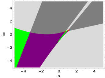
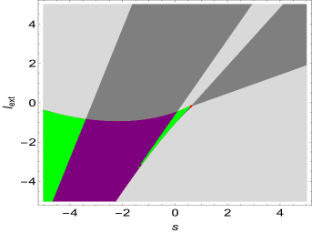
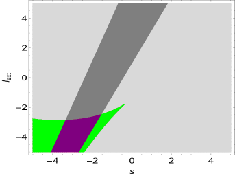
(i)   (ii)
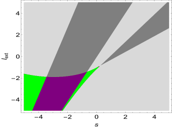
(iii) (iv)

Figure 2: Stability maps of the equilibrium points $E$, in the plane $s-I_{ext}$, for $k=0$ (i), $k=5$ (ii), $k=10$ (iii) and $k=15$ (iv). The colored regions correspond to one equilibrium point [unstable (dark-gray), stable (light-gray)] and three equilibrium points [1 unstable (green), 2 unstable (purple), all unstable (red)]. The latter only appears, within the resolution of the figure, near the vertex of region (A).

Let us start by analyzing the case where the neuronal model is not subjected to any magnetic flux (i.e., $k=0$), which is depicted in Fig. 2.i). In region (B), we distinguish the subregions where the single equilibrium point is unstable (dark-gray) or stable (light-gray), Region (A) is mainly composed of two subdomains (green and purple), where, among the three equilibrium points defined by $(s,I_{ext})$, only one is unstable (green), or two are unstable (purple). A small subdomain (red) where the the three equilibrium points are all unstable is also observed near the vertex of region (A).

In region (B), a stable fixed point means extinction of the oscillations. Taking into account the electromagnetic induction, with intensity $k$, clearly the region (B) gains stability with increasing $k$, as can be observed by the expansion of the light-gray region, in the successive panels of Fig. 2.

Besides the reduction of region (A), when $k$ increases, there is also a gain of stability, as can be seen by the predominance of the green subdomain over the purple one, and disappearance of the small red subdomain associated to three unstable fixed points. In short, the progressive increase of magnetic coupling tends to reduce the number of equilibrium points form 3 to 1 and turns the single equilibrium point more stable. Recall that $r=0.001$ is used, but a similar portrait to that shown in Fig. 2 is observed for other values of $0<r\lesssim 0.1$.

Illustrative examples are provided in the tables of Appendix C, where, for selected points $P=(s,I_{ext})$, we present the corresponding equilibrium states (whose number depends on the region which $P$ belongs to) and their corresponding eigenvalues, which express the nature of the fixed points. For comparison, for each point $P$, results are given for the neuronal MHR system with $k=0$ and $k=10$.

III.3 Bifurcation diagrams

We present, in this section, bifurcation diagrams in the MHR model, as a function of the control parameters. Trajectories were obtained solving numerically Eq. (2), using a $4th$-order Runge-Kutta algorithm, typically starting from the initial condition $(x,y,z,\phi)_{t=0}=(0,0,0,0)$, and performing measurements in the interval $t\in(1000,8000)$. We also computed the largest Lyapunov exponent, defined by

$$L_{max}=\lim_{t\to\infty\atop\delta{X}(0)\to 0}\frac{1}{t}\ln\left|\frac{\delta{X}(t)}{\delta{X}(0)}\right|,$$ (12)

where ${X}$ is the state of the system and in this case $\delta{X}$ is the separation vector between two close trajectories. $L_{max}$ is estimated using Benettin algorithm, after solving numerically Eq. (2) and its associated variational equation.

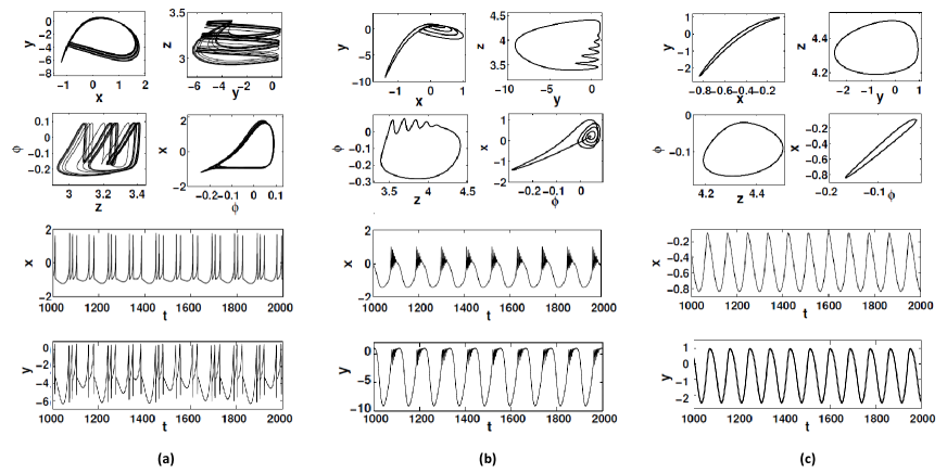
Figure 3: Projections of the phase portrait in different planes, and corresponding time series for the membrane potential $x$ and the current $y$ vs. $t$, for (a) $k=0$, (b) $k=5$ and (c) $k=10$, with $r=0.008$, $s=4$ and $I_{ext}=3.25$. In (a), we observe the chaotic attractor of the HR neuronal model, while the dynamics becomes regularized as $k$ increases.

Figure 3 shows the projections of the phase portrait in different planes, as well as the time series for the membrane potential $x$, and the recovery current $y$, for different values of $k$. When $k=0$, the well-known chaotic attractor of the neuronal HR model yamapi13 ; parastesh18 ; rajagopal19 is recovered (Fig. 3a), while as $k$ increases, the dynamics becomes more and more regular, the amplitude of the spikes per burst is reduced (e.g., Fig. 3b) and disappears for large enough $k$ (e.g., Fig. 3c). The change in patterns can affect the performance of the neuron, impacting on information processing and transmission.

In Fig. 4 we present a heat-plot of the largest Lyapunov exponent in the plane $r-k$, which provides a full picture of the effects of magnetic induction on the dynamics of the MHR, illustrated for particular values of the strength $k$ in Fig. 3.

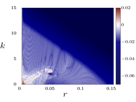
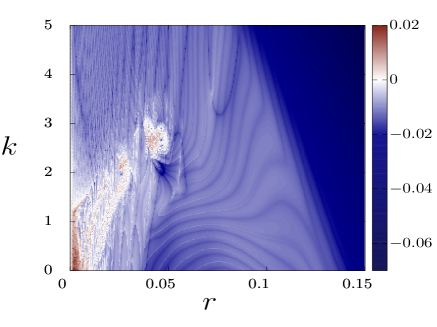
Figure 4: Heat-plots of the largest Lyapunov exponent $L_{max}$ as a function of $r$ and $k$, using $s=4$, $I_{ext}=3.25$. In the right-hand-side panel we amplified the low $k$ region. We observe that for sufficiently low $k$ chaotic trajectories (red scale) can exist when $r$ is also low, but increasing $k$ leads to negative values of $L_{max}$, indicating regular behavior. The darker blue region corresponds to damped oscillations towards a fixed point.

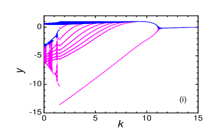
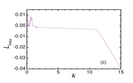
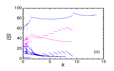
Figure 5: Bifurcation diagrams and the largest Lyapunov exponent as a function of $k$, for $r=0.008$, with $s=4$, $I_{ext}=3.25$. (i) In these and following bifurcation diagrams, magenta and blue lines correspond respectively to the local minima and maxima of the timeseries $y(t)$, (ii) largest Lyapunov exponent. (iii) interspike intervals: time elapsed between maxima (blue) and between minima (magenta). After approx. $k>9$, the single value corresponds to the period of simple oscillations, which become damped near $k>11$.

Further details on the effects of varying $k$ are presented through the bifurcation diagrams for the recovery current. In Fig. 5, we use $k$ as bifurcation parameter when $r=0.008$. Besides the diagram for the extreme values in Fig. 5(i), we also show the corresponding plot of the largest Lyapunov exponent $L_{max}$ in Fig. 5(ii). For $k>11$, the dynamics tends to a fixed point, characterized by a negative exponent (dark blue region in the diagrams of Fig. 4). We also present the diagram for interspike intervals, $ISI$ as function of $k$, in Fig. 5(iii). The time intervals between consecutive maxima (minima) of $y(t)$ are ploted in blue (magenta). The larger values between maxima correspond to the quiescent intervals, while the smaller ones are intraburst interspike intervals. For small $k$ the chaotic windows are also reflected in ISI. A single value means simple periodic oscillations as those illustrated in Fig. 3(c), that occur approximately within $9<k<11$, above that interval, oscillations are damped (tending to a constant value) but still detected by our code until the amplitude is so small that the machine precision is attained. As $k$ increases, the chaotic windows disappear, and $L_{max}$ becomes negative for $k\gtrsim 2$. Moreover, the characteristic time between spikes changes with $k$. At At $k\simeq 9$, simple periodic oscillations (without multiple spikes) occur, and at $k\simeq 11$ oscillations are lost, which means drastic consequences on neuron performance. Cuts for other values of $r$ (0.001 and 0.05) are presented in Appendix D, complementing the information of the heat-plots of Fig. 4.

In the following figures  6-8, we compare the bifurcation diagrams in the absence ($k=0$) and presence ($k=5$) of electromagnetic induction, using $r$, $s$ and $I_{ext}$ as bifurcation parameters, respectively. The local maxima (blue) and minima (magenta) of the timeseries are distinguished. The corresponding plots for the largest Lyapunov exponent $L_{max}$ are also shown.

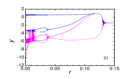
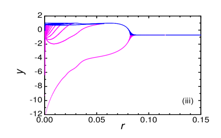
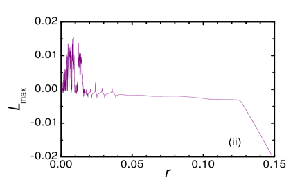
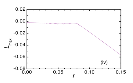
Figure 6: Bifurcation diagrams and the largest Lyapunov exponent as a function of $r$, for $k=0$ (i)-(ii) and $k=5$ (iii)-(iv), with $s=4$, $I_{ext}=3.25$. In these and following bifurcation diagrams, magenta and blue lines correspond respectively to the local minima and maxima of the timeseries $y(t)$.

For the bifurcation parameter $r$, which rules the slow dynamics, we show Fig. 6. In the case $k=0$, corresponding to Figs. 6.i and  6.ii, we observe chaotic intervals, interrupted by regularity windows. In particular, a reverse period-doubling transition occurs. Therefore, decreasing the value of parameter $r$ can induce a complex sequence of period-doubling bifurcations, resulting in the duplication of spikes. When the electromagnetic radiation is taken into account, with intensity $k=5$, as shown in Figs. 6.iii and  6.iv, the neuronal model no longer exhibits complex behaviors, and we find only periodic oscillations. The diagrams for intermediate values of $k$, showing how increasing $k$ extinguishes the chaotic windows, are presented in the Appendix D.

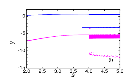
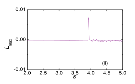
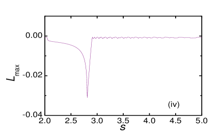
Figure 7: Bifurcation diagrams and the largest Lyapunov exponent as a function of $s$, for $k=0$ (i)-(ii) and $k=5$ (iii)-(iv), with $r=0.001$, $I_{ext}=3.25$. (For $s<3.0$ in (iii), a transient longer than $10^{4}$ was discarded, indicating a slow relaxation.)

Bifurcation diagrams are also shown for the control parameters $s$ ( Fig. 7) and $I_{ext}$ (Fig. 8). As a function of $s$, oscillations with several spikes appear at $s\approx 4$ when $k=0$. The peak of $L_{max}$ at $s\simeq 3.9$ is a reflection of the transition between two different oscillatory regimes. For $k=5$, the oscillations occur for smaller $s\simeq 2.9$ but the amplitude of the spikes is diminished. This reduction of spike amplitude is also observed as a function of $I_{ext}$, in Fig. 8.

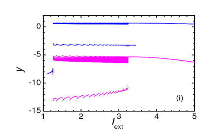
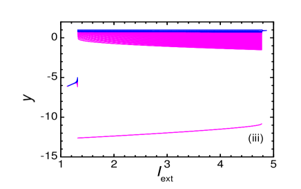
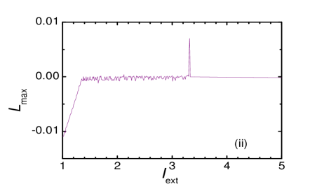
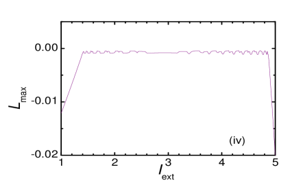
Figure 8: Bifurcation diagrams and the largest Lyapunov exponent as a function of $I=I_{ext}$, for $k=0$ (i)-(ii) and $k=5$ (iii)-(iv), with $r=0.001$, $s=4$.

Therefore, when electromagnetic induction is present, we observe the tendency that the chaotic windows disappears and the neuron exhibits regular spikes.

IV Conclusions

We have performed a stability analysis of the Hindmarsh-Rose neuronal, extended to take into account the effect of the magnetic flux on the membrane potential (MHR model) lv16 . In Section III, we have shown the effects of electromagnetic induction on neuronal dynamics by varying the magnetic coupling $k$. We noted that the domain of existence of three equilibrium points in the plane $s-I_{ext}$ decreased drastically when increasing $k$, leading to a dynamics with a single equilibrium point. Moreover, unstable points become progressively stable when $k$ increases, spoiling oscillations. The observed bifurcations in the neuronal dynamics reveal a complex structure when the parameters $(I_{ext},r,s)$ are changed in the absence of magnetic induction. Variations of the maximal Lyapunov exponent, bifurcations diagrams, phase portraits, and time series allowed to emphasize the stabilizing and regularizing role of the introduction of electromagnetic induction on the neuron dynamics, for the values of the parameters considered.

Our results can be relevant as basis for future studies on networks of MHR neurons. As possible extensions, it would be also interesting to analyze the effect of different kinds of additive and multiplicative noises, as well as time-delays in the responses of the neuron.

Data availability statements

The data from simulations that support the findings of this study are available on request from the corresponding author, RY.

Appendix A Equilibrium points

With the change of variables $x_{e}=t-a_{1}/(3a_{0})$, Eq. (4) becomes reduced to $t^{3}+pt+q=0$, where $p=(3a_{0}a_{2}-a_{1}^{2})/(3a_{0}^{2})$ and $q=(2a_{1}^{3}-9a_{0}\,a_{1}\,a_{2}+27a_{0}^{2}a_{3})/(27a_{0}^{3})$. To obtain its roots, we define the discriminant $\Delta=q^{2}+\frac{4}{27}p^{3}$, which, after substitution of the coefficients defined in Eq. (5), explicitly becomes

$$\Delta=\left[\dfrac{2(b-d)^{3}-9T(b-d)(s+k\alpha)}{27T^{3}}+\frac{c+sx_{0}+I_{ext}}{T}\right]^{2}+\frac{4}{27}\left[\dfrac{3T(s+k\alpha)-(b-d)^{2}}{3T^{2}}\right]^{3}\,.\;\;\;\;\;$$

(13)

The signal of $\Delta$ determines the number of real roots. Then, setting $\Delta=0$, we extracted the expression $I_{ext}^{\pm}(s)$ in Eq. (6), that delimits the regions with three (A) and one (B) real-valued roots.

The real-valued solutions $x_{e}$ of Eq. (4) yield the equilibrium points of the form

$$E=(x_{e},y_{e},z_{e},\phi_{e})=(x_{e},-dx_{e}^{2}+c,s(x_{e}-x_{0}),k_{1}x_{e}/k_{2})\,.$$ (14)

1. If $\Delta$ < 0, corresponding to region (A) in Fig. 1, there are three equilibrium points $E_{1}=(x_{e1},y_{e1},z_{e1},\phi_{e1})$, $E_{2}=(x_{e2},y_{e2},z_{e2},\phi_{e2})$ and $E_{3}=(x_{e3},y_{e3},z_{e3},\phi_{e3})$, given by:

   $$x_{ek}=2\sqrt{-\frac{p}{3}}\cos\left(\frac{1}{3}\arccos\left(\frac{-q}{\sqrt{-4p^{3}/27}}\right)-\frac{2\pi(k-1)}{3}\right)+\dfrac{b-d}{3T}\;\;\;\;\;\mbox{for $k=1,2,3$}\,.$$

   (15)

2. If $\Delta$ > 0, corresponding to the region (B) in Fig. 1, there is only one real root, then the system has a single equilibrium point $E=(x_{e},y_{e},z_{e},\phi_{e})$ defined by

   $$x_{e}=\sqrt[3]{\dfrac{-q+\sqrt{\Delta}}{2}}+\sqrt[3]{\dfrac{-q-\sqrt{\Delta}}{2}}+\dfrac{b-d}{3T}.$$ (16)

3. If $\Delta$ = 0 (borderlines in Fig. 1), there are two equilibrium points, $E_{1}=(x_{e1},y_{e1},z_{e1},\phi_{e1})$ and $E_{2}=(x_{e2},y_{e2},z_{e2},\phi_{e2})$, defined by

   $$x_{e1}=2\sqrt[3]{\dfrac{-q}{2}}+\dfrac{b-d}{3T},\;\;\;\;\;\;\mbox{and}\;\;\;\;\;\;x_{e2}=-\sqrt[3]{\dfrac{-q}{2}}+\dfrac{b-d}{3T}.$$ (17)

Appendix B Coefficients of the characteristic polynomial

Here we give the explicit expressions of the coefficients $\delta_{i}$, with $1\leq i\leq 4$, of the characteristic polynomial in Eq. (10), associated to the Jacobian matrix (9):

$$\delta_{1} = 3\beta kk_{1}^{2}x_{e}^{2}/k_{2}^{2}+3ax_{e}^{2}+{\alpha}k-2bx_{e}+k_{2}+r+1,$$

$$\delta_{2} = 3ak_{2}x_{e}^{2}+3arx_{e}^{2}+3ax_{e}^{2}+{\alpha}kk_{2}+r({\alpha}k+s)-2brx_{e}$$

$$+ {\alpha}k-2bk_{2}x_{e}+2(d-b)x_{e}+k_{2}r+k_{2}+r$$

$$+ 3\beta kk_{1}^{2}x_{e}^{2}[3k_{2}+r+1]/k_{2}^{2},$$

$$\delta_{3} = 3ak_{2}rx_{e}^{2}+3ak_{2}x_{e}^{2}+3arx_{e}^{2}+\alpha kk_{2}r-2bk_{2}rx_{e}+\alpha kk_{2}$$

$$+ r(\alpha k+s)+2(d-b)k_{2}x_{e}+2(d-b)rx_{e}+k_{2}rs+k_{2}r$$

$$+ 3\beta kk_{1}^{2}x_{e}^{2}\,[3k_{2}r+3k_{2}+r]/k_{2}^{2},$$

$$\delta_{4} = r\,k_{2}\,[9\beta kk_{1}^{2}x_{e}^{2}/k_{2}^{2}+3ax_{e}^{2}+\alpha k+s+2(d-b)x_{e}].$$

Appendix C Nature of the equilibrium points

In the following tables, for chosen points $P$ in the plane $s-I_{ext}$ (Fig. 2), we present the associated equilibrium point(s) $E$, together with the corresponding eigenvalues of the Jacobian matrix, emphasizing (in the last column) the nature of the equilibrium points, for $k=0$ (Table 1) and $k=10$ (Table 2).

Table 1: Case $k=0$. Equilibrium points and corresponding eigenvalues.

$\;\;\;\;P=\left({\begin{array}[]{*{20}{c}}s\\ I_{ext}\end{array}}\right)\;\;\;\;$	Equilibrium point $E=(x_{e},y_{e},z_{e},\phi_{e})$	Eigenvalues of $J(x_{e},y_{e},z_{e},\phi_{e})$	Nature of the equilibrium point
${P_{1}}=\left({\begin{array}[]{*{20}{c}}-2\\ 1\end{array}}\right)$	$E_{1}=(1.53,-10.74,-6.30,0.31)$	$\begin{array}[]{*{20}{l}}{{\lambda_{1}}={0.578+3.57i}}\\ {{\lambda_{2}}={0.578-3.57i}}\\ {{\lambda_{3}}={-0.5}}\\ {{\lambda_{4}}={-8.4\times 10^{-4}}}\end{array}$	saddle-focus
${P_{2}}=\left({\begin{array}[]{*{20}{c}}1.5\\ 1\end{array}}\right)$	$E_{2}=(-0.77,-2.01,1.26,-0.15)$	$\begin{array}[]{*{20}{l}}{{\lambda_{1}}={-7.63}}\\ {{\lambda_{2}}={-0.49}}\\ {{\lambda_{3}}={0.16}}\\ {{\lambda_{4}}={1.57\times 10^{-4}}}\end{array}$	saddle point
	$E_{3a}=(-2.57,-32.0,4.75,-0.51)$	$\begin{array}[]{*{20}{l}}{{\lambda_{1}}={-35.9}}\\ {{\lambda_{2}}={-0.5}}\\ {{\lambda_{3}}={-0.26}}\\ {{\lambda_{4}}={-4.7\times 10^{-4}}}\end{array}$	stable node
${P_{3}}=\left({\begin{array}[]{*{20}{c}}-5\\ 0\end{array}}\right)$	$E_{3b}=(2.19,-22.9,-19.0,0.44)$	$\begin{array}[]{*{20}{l}}{{\lambda_{1}}={{-1.11}+4.67i}}\\ {{\lambda_{2}}={{-1.11}-4.67i}}\\ {{\lambda_{3}}={-0.5}}\\ {{\lambda_{4}}={-7.8\times 10^{-4}}}\end{array}$	stable saddle-focus
	$E_{3c}=(-1.61,-12.1,0.0,-0.32)$	$\begin{array}[]{*{20}{l}}{{\lambda_{1}}={-18.5}}\\ {{\lambda_{2}}={-0.5}}\\ {{\lambda_{3}}={0.078}}\\ {{\lambda_{4}}={0.0025}}\end{array}$	saddle point
	$E_{4a}=(-2.41,-28.01,2.37,-0.48)$	$\begin{array}[]{*{20}{l}}{{\lambda_{1}}={-32.62}}\\ {{\lambda_{2}}={-0.5}}\\ {{\lambda_{3}}={-0.24}}\\ {{\lambda_{4}}={-6.1\times 10^{-4}}}\end{array}$	stable node
${P_{4}}=\left({\begin{array}[]{*{20}{c}}-3\\ -1\end{array}}\right)$	$E_{4b}=(1.64,-12.43,-9.77,0.328)$	$\begin{array}[]{*{20}{l}}{{\lambda_{1}}={{0.39}+3.80i}}\\ {{\lambda_{2}}={{0.39}-3.80i}}\\ {{\lambda_{3}}={-0.5}}\\ {{\lambda_{4}}={-7.9\times 10^{-4}}}\end{array}$	saddle-focus
	$E_{4c}=(-1.23,-6.56,-1.16,-0.246)$	$\begin{array}[]{*{20}{l}}{{\lambda_{1}}={-12.95}}\\ {{\lambda_{2}}={-0.5}}\\ {{\lambda_{3}}={0.0359}}\\ {{\lambda_{4}}={-0.00726}}\end{array}$	saddle point
	$E_{5a}=(1.54,-10.97,-9.49,0.309)$	$\begin{array}[]{*{20}{l}}{{\lambda_{1}}={0.56+3.59i}}\\ {{\lambda_{2}}={0.56-3.59i}}\\ {{\lambda_{3}}={-0.5}}\\ {{\lambda_{4}}={-7.74\times 10^{-4}}}\end{array}$	saddle-focus
${P_{5}}=\left({\begin{array}[]{*{20}{c}}-3\\ -2\end{array}}\right)$	$E_{5b}=(-2.58,-32.37,2.89,-0.516)$	$\begin{array}[]{*{20}{l}}{{\lambda_{1}}={-36.1}}\\ {{\lambda_{2}}={-0.5}}\\ {{\lambda_{3}}={-0.266}}\\ {{\lambda_{4}}={-6.88\times 10^{-4}}}\end{array}$	stable node
	$E_{5c}=(-0.963,-3.64,-1.96,-0.192)$	$\begin{array}[]{*{20}{l}}{{\lambda_{1}}={-9.67}}\\ {{\lambda_{2}}={-0.5}}\\ {{\lambda_{3}}={0.11}}\\ {{\lambda_{4}}={-3.7\times 10^{-3}}}\end{array}$	saddle point

Table 2: Case $k=10$. Equilibrium points and corresponding eigenvalues.

$P=\left({\begin{array}[]{*{20}{c}}s\\ I_{ext}\end{array}}\right)$	Equilibrium point $E=(x_{e},y_{e},z_{e},\phi_{e})$	Eigenvalues of $J(x_{e},y_{e},z_{e},\phi_{e})$	Nature of the equilibrium point
$\;\;\;\;{P_{1}}=\left({\begin{array}[]{*{20}{c}}-2\\ 1\end{array}}\right)\;\;\;\;$	$E_{1}=(1.379,-8.5,-5.99,0.275)$	$\begin{array}[]{*{20}{l}}{{\lambda_{1}}={0.21+3.52i}}\\ {{\lambda_{2}}={0.21-3.52i}}\\ {{\lambda_{3}}={-0.505}}\\ {{\lambda_{4}}={-8.41\times 10^{-4}}}\end{array}$	saddle-focus
${P_{2}}=\left({\begin{array}[]{*{20}{c}}1.5\\ 1\end{array}}\right)$	$E_{2}=(-0.199,0.801,2.12,-0.039)$	$\begin{array}[]{*{20}{l}}{{\lambda_{1}}={-3.21}}\\ {{\lambda_{2}}={-0.0989}}\\ {{\lambda_{3}}={-0.0057}}\\ {{\lambda_{4}}={-0.498}}\end{array}$	stable node
${P_{3}}=\left({\begin{array}[]{*{20}{c}}-5\\ 0\end{array}}\right)$	$E_{3}=(1.79,-15.0,-17.0,0.36)$	$\begin{array}[]{*{20}{l}}{{\lambda_{1}}={-0.54+4.23i}}\\ {{\lambda_{2}}={-0.54-4.23i}}\\ {{\lambda_{3}}={-0.51}}\\ {{\lambda_{4}}={-7.3\times 10^{-4}}}\end{array}$	stable node-focus
${P_{4}}=\left({\begin{array}[]{*{20}{c}}-3\\ -1\end{array}}\right)$	$E_{4}=(1.32,-7.76,-8.83,0.265)$	$\begin{array}[]{*{20}{l}}{{\lambda_{1}}={0.282+3.426}i}\\ {{\lambda_{2}}={0.282-3.426}i}\\ {{\lambda_{3}}={-0.505}}\\ {{\lambda_{4}}={-7.49\times 10^{-4}}}\end{array}$	saddle-focus
	$E_{5a}=(1.37,-8.5,-8.9,0.27)$	$\begin{array}[]{*{20}{l}}{{\lambda_{1}}={0.229+3.51i}}\\ {{\lambda_{2}}={0.229-3.51i}}\\ {{\lambda_{3}}={-7.6\times 10^{-4}}}\\ {{\lambda_{4}}={-0.00194}}\end{array}$	saddle-focus
${P_{5}}=\left({\begin{array}[]{*{20}{c}}-3\\ -2\end{array}}\right)$	$E_{5b}=(-1.77,-14.78,0.477,-0.355)$	$\begin{array}[]{*{20}{l}}{{\lambda_{1}}={-22.7}}\\ {{\lambda_{2}}={-0.4832}}\\ {{\lambda_{3}}={-0.187}}\\ {{\lambda_{4}}={-2.48\times 10^{-4}}}\end{array}$	stable node
	$E_{5c}=(-1.46,-9.76,-0.451,-0.293)$	$\begin{array}[]{*{20}{l}}{{\lambda_{1}}={-17.3}}\\ {{\lambda_{2}}={-0.487}}\\ {{\lambda_{3}}={-0.122}}\\ {{\lambda_{4}}={4.5\times 10^{-4}}}\end{array}$	saddle point

Appendix D Bifurcation diagrams

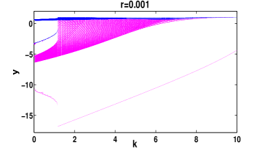
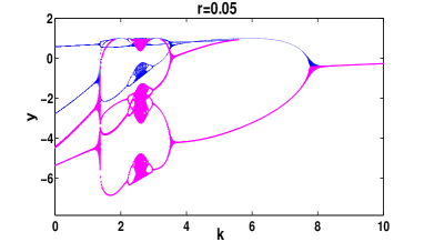
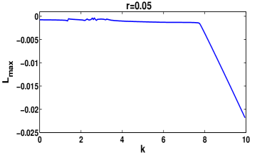
(i) (iii)
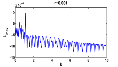
(ii) (iv)

Figure D1: Bifurcation diagrams and the largest Lyapunov exponent as a function of $k$, for $r=0.001$ (i)-(ii) and $r=0.05$ (iii)-(iv), with $s=4$, $I_{ext}=3.25$. Magenta and blue lines correspond respectively to the local minima and maxima of the timeseries $y(t)$.

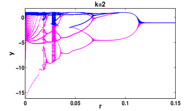
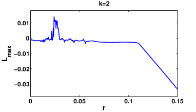
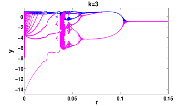
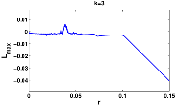
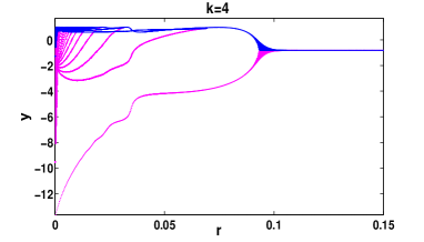
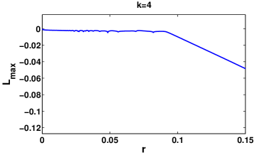
Figure D2: Bifurcation diagram and $L_{max}$ as a function of $r$, for each value of the intensity of the magnetic flux $k$ indicated in the legends. We used $s=4$, $I_{ext}=3.25$, as in Fig. 6.

References

- (1) Hodgkin, A.L., Huxley, A.F.: A quantitative description of membrane current and its application to conduction and excitation in nerve, J. Physiol. (Lond.) 117, 500–544 (1952). https://doi.org/10.1113/jphysiol.1952.sp004764
- (2) Hasegawa, H.: Responses of a Hodgkin-Huxley neuron to various types of spike-train inputs, Phys. Rev. E 61, 718 (2000). https://doi.org/10.1103/PhysRevE.61.718
- (3) Kang, Q., Huang, B. Y., Zhou, M. C.: Dynamic behavior of artificial Hodgkin–Huxley neuron model subject to additive noise, IEEE Trans. Cybern. 46, 2083 (2015). https://doi.org/10.1109/TCYB.2015.2464106
- (4) Morris, C., Lecar, H.: Voltage oscillations in the barnacle giant muscle fiber, Biophys. J. 35(1):193–213, (1981). https://doi.org/10.1016/s0006-3495(81)84782-0
- (5) Hu, X., Liu, C., Liu, L., Ni, J., Li, S.: An electronic implementation for Morris–Lecar neuron model, Nonlinear Dyn. 84, 2317 (2016). https://doi.org/10.1007/s11071-016-2647-y
- (6) Shi, M., Wang, Z.: Abundant bursting patterns of a fractional-order Morris–Lecar neuron model, Commun Nonlinear Sci. Numer. Simulat. 19, 1956 (2014). https://doi.org/10.1016/j.cnsns.2013.10.032
- (7) Izhikevich, E.M.: Simple model of spiking neurons, IEEE Trans. Neural Networks, 14(6):1569 (2003). https://doi.org/10.1109/TNN.2003.820440
- (8) Kosmidis, E. K., Pakdaman, K.: An analysis of the reliability phenomenon in the FitzHugh-Nagumo model, J. Comput. Neurosci. 14, 5 (2003). https://doi.org/10.1023/a:1021100816798
- (9) Abbasian, A. H., Fallah, H., Razvan, M. R.: Symmetric bursting behaviors in the generalized FitzHugh-Nagumo model, Biol. Cybern. 107, 465 (2013). https://doi.org/10.1007/s00422-013-0559-1
- (10) Wang, J., Zhang, T., Deng, B.: Synchronization of FitzHugh–Nagumo neurons in external electrical stimulation via nonlinear control, Chaos, Solitons and Fractals 31, 30 (2007). http://dx.doi.org/10.1016/j.chaos.2005.09.006
- (11) Hindmarsh, J.L., Rose, R.M.: A model of the nerve impulse using two first-order differential equations, Nature 296, 162–164 (1982). https://doi.org/10.1038/296162a0
- (12) Hindmarsh, J.L., Rose, R.M.: A model of neuronal bursting using three coupled first order differential equations, Proc. R. Soc. Lond. B 221(1222), 87-102 (1984). https://doi.org/10.1098/rspb.1984.0024
- (13) Innocenti, G., Morelli, A., Genesio, R., Torcini, A., Dynamical phases of the Hindmarsh-Rose neuronal model: studies of the transition from bursting to spiking chaos, Chaos 17, 043128-1 (2007). https://doi.org/10.1063/1.2818153
- (14) Wu, K., Luo, T., Lu, H., Wang, Y.: Bifurcation study of neuron firing activity of the modified Hindmarsh–Rose model, Neural Comput. Applic. 27, 739 (2016). https://doi.org/10.1007/s00521-015-1892-1
- (15) Zhou, P., Yao, Z., Ma J., Zhu, Z., A piezoelectric sensing neuron and resonance synchronization between auditory neurons under stimulus, Chaos, Solitons & Fractals 145, 110751 (2021).
- (16) Zhang, Z., Ma J., Wave filtering and firing modes in a light-sensitive neural circuit, Appl. Phys.& Eng.) 22(9):707-720 (2021).
- (17) Houart, G., Dupont, G., Goldbeter, A.: Bursting, chaos and birhythmicity originating from self-modulation of the inositol 1,4,5-trisphosphate signal in a model for intracellular Ca2+ oscillations, Bull. Math. Biol. 61(3), 507-530 (1999). https://doi.org/10.1006/bulm.1999.0095
- (18) Izhikevich, E.M.: Neural excitability, spiking and bursting, Int. J. Bifurc. Chaos 10(6), 1171–1266 (2000). https://doi.org/10.1142/S0218127400000840
- (19) Bao, B.C., Liu, Z., Xu, J.P.: Steady periodic memristor oscillator with transient chaotic behaviors, Electron. Lett. 46, 228-230 (2010). https://doi.org/10.1049/el.2010.3114
- (20) Muthuswamy, B.: Implementing memristor based chaotic circuits, Int. J. Bifurc. Chaos 20, 1335-1350 (2010). https://doi.org/10.1142/S0218127410026514
- (21) Li, Q.D., Zeng, H.Z., Li, J.: Hyperchaos in a 4D memristive circuit with infinitely many stable equilibria, Nonlinear Dyn. 79, 2295-2308 (2015). https://doi.org/10.1007/s11071-014-1812-4
- (22) Wu, F., Wang, C., Xu, Y., Ma, J.: Model of electrical activity in cardiac tissue under electromagnetic induction, Sci. Rep. 6:28, (2016). https://doi.org/10.1038/s41598-016-0031-2
- (23) Xu, Y., Jia, Y., Ge, M., Lu, L., Yang, L., Zhan, X.: Effects of ion channel blocks on electrical activity of stochastic Hodgkin-Huxley neural network under electromagnetic induction, Neurocomp. 283(29):196–204, (2018). https://doi.org/10.1016/j.neucom.2017.12.036
- (24) Wu, F.Q., Wang, C.N., Jin, W.Y., Ma, J.: Dynamical responses in a new neuron model subjected to electromagnetic induction and phase noise, Physica A 469, 81–88, (2017). https://doi.org/10.1016/j.physa.2016.11.056
- (25) Lv, M.,Wang, C., Ren, G., Ma, J., Song, X.: Model of electrical activity in a neuron under magnetic flow effect, Nonlinear Dyn. 85:1479–1490 (2016). https://doi.org/10.1007/s11071-016-2773-6
- (26) Wu, J., Xu, Y., Ma, J.: Lévy noise improves the electrical activity in a neuron under electromagnetic radiation, PLOS ONE, 12(3):e017330, (2017). https://doi.org/10.1371/journal.pone.0174330
- (27) Usha, K., Subha, P.A.: Hindmarsh-Rose neuron model with memristors, BioSystems 178, 1-9 (2019). https://doi.org/10.1016/j.biosystems.2019.01.005
- (28) Parastesh, F., Rajagopal, K., Karthikeyan, A., Alsaedi, A., Hayat, T.,Pham, V.-T.: Complex dynamics of a neuron model with discontinuous magnetic induction and exposed to external radiation, Cognit. Neurodyn. 12(6), 607–614, (2018). https://doi.org/10.1007/s11571-018-9497-x
- (29) Parastesh, F., Rajagopal, K., Karthikeyan, A., Alsaadi, F.E.,Hayat, T., Pham, V.-T., Hussain, I.: Birth and death of spiral waves in a network of Hindmarsh–Rose neurons with exponential magnetic flux and excitable media, Appl. Math. Comput. 354, 377–384 (2019). http://doi.org/10.1016/j.amc.2019.02.041
- (30) Mostaghimi, S., Nazarimehr, F., Jafari, S., Ma, J.: Chemical and electrical synapse-modulated dynamical properties of coupled neurons under magnetic flow, Appl. Math. Comput. 348, 42–56 (2019). http://dx.doi.org/10.1016/j.amc.2018.11.030
- (31) Majhi, S., Ghosh, D.: Alternating chimeras in networks of ephaptically coupled bursting neurons, Chaos 28, 083113 (2018). https://doi.org/10.1063/1.5022612
- (32) Kundu, S., Bera, B.K., Ghosh, D., Lakshmanan, M., Chimera patterns in three-dimensional locally coupled systems, Phys. Rev. E 99, 022204 (2019). https://doi.org/10.1103/PhysRevE.99.022204
- (33) Makarov V.V, Kundu, S., Kirsanov, D.V., Frolov, N.S., Maksimenko, V.A., Ghosh, D., Dana, S.K. Hramov, A.E., Multiscale interaction promotes chimera states in complex networks, Commun Nonlinear Sci Numer Simulat 71 118–129 (2019). https://doi.org/10.1016/j.cnsns.2018.11.015
- (34) Wang, H., Wang, Q., Lu, Q., Zheng, Y.: Equilibrium analysis and phase synchronization of two coupled HR neurons with gap junction, Cognit. Neurodyn. 7(2), 121-131 (2013). https://doi.org/10.1007/s11571-012-9222-0
- (35) Rajagopal, K., Khalaf, A.J.M., Parastesh, F., Moroz, I., Karthikeyan, A.,Jafari, S.: Dynamical behavior and network analysis of an extended Hindmarsh-Rose neuron model, Nonlinear Dynamics 98, 477–487 (2019). https://doi.org/10.1007/s11071-019-05205-0
- (36) Dtchetgnia Djeundam, S.R., Yamapi, R., Kofane, T.C., Aziz-Alaoui, : Deterministic and stochastic bifurcations in the Hindmarsh-Rose neuronal model with and without random signal, Chaos 23, 033125 (2013). https://doi.org/10.1063/1.4818545
- (37) Megam Ngouonkadi, E.B., Fotsin, H.B., Louodop Fotso, P., Kamdoum Tamba, V., Cerdeira, H.A.: Bifurcations and multistability in the extended Hindmarsh–Rose neuronal oscillator, Chaos, solitons and fractals, 85, 151 (2016). http://dx.doi.org/10.1016/j.chaos.2016.02.001
- (38) Hayashi, C.: Nonlinear oscillations in physical systems (McGraw-Hill, New York (1964). https://doi.org/10.1515/9781400852871