Scalable Bicriteria Algorithms for Non-Monotone Submodular Cover

Abstract

In this paper, we consider the optimization problem Submodular Cover (SC), which is to find a minimum cost subset of a ground set $U$ such that the value of a submodular function $f$ is above a threshold $\tau$. In contrast to most existing work on SC, it is not assumed that $f$ is monotone. Two bicriteria approximation algorithms are presented for SC that, for input parameter $0<\epsilon<1$, give $O(1/\epsilon^{2})$ ratio to the optimal cost and ensures the function $f$ is at least $\tau(1-\epsilon)/2$. A lower bound shows that under the value query model shows that no polynomial-time algorithm can ensure that $f$ is larger than $\tau/2$. Further, the algorithms presented are scalable to large data sets, processing the ground set in a stream. Similar algorithms developed for SC also work for the related optimization problem of Knapsack Constrained Submodular Maximization (KCSM). Finally, the algorithms are demonstrated to be effective in experiments involving graph cut and data summarization functions.

1 Introduction

Submodular set functions arise in many applications such as summarization of data sets (Tschiatschek et al., 2014), feature selection in machine learning (Das and Kempe, 2018), cut functions in graphs (Balkanski et al., 2018), viral marketing in a social network (Kempe et al., 2003), and many others. Intuitively, submodularity describes a diminishing returns property of set functions. Formally, let $f:2^{U}\to\mathbb{R}$ be defined over subsets of a universe $U$ of size $n$. Then $f$ is submodular if for all $A\subseteq B\subseteq U$ and $x\notin B$, $f(A\cup\{x\})-f(A)\geq f(B\cup\{x\})-f(B)$. Moreover, $f$ is monotone if for all $A\subseteq B\subseteq U$, $f(A)\leq f(B)$. In this paper, the Submodular Cover problem (SC) is considered.

Problem 1 (SC).

Define submodular $f:2^{U}\to\mathbb{R}_{\geq 0}$ over subsets of the universe $U$ of size $n$, and non-negative cost function $w:U\to\mathbb{R}_{\geq 0}$. Given threshold $\tau\leq\max\{f(X):X\subseteq U\}$, find

$$\text{argmin}_{X\subseteq U}\left\{\sum_{x\in X}w(x):f(X)\geq\tau\right\}.$$

Let $OPT$ refer to the cost of the optimal solution.

The SC formulation captures applications where we wish to ensure that a submodular function $f$ is sufficiently high, while minimizing cost. When $f$ is monotone, SC has been studied extensively, e.g. Wolsey (1982); Mirzasoleiman et al. (2015, 2016); Norouzi-Fard et al. (2016). To the best of our knowledge, the only work to consider SC with non-monotone $f$ is Iyer and Bilmes (2013), discussed in Section 2 below. Therefore, non-monotone SC is relatively unexplored, despite such problems arising in learning applications.

For example, non-monotone submodular functions frequently arise in data summarization tasks as a measure of how effectively a subset $X\subseteq U$ summarizes a data set $U$ (Gillenwater et al., 2012; Tschiatschek et al., 2014) . Data summarization can then be formulated as an instance of SC where we seek to pick the summary of minimum memory (e.g. if $U$ is images then the cost $w$ may be the size of each image) that reaches a constant factor of the maximum value of $f$ (i.e. $\tau=\xi\max_{X\subseteq U}f(X)$). As a second example, non-monotone, submodular revenue functions may be formulated on a social network (Hartline et al., 2008; Balkanski et al., 2018). In this context, the SC problem asks to guarantee a certain amount of revenue with minimum cost.

The above examples demonstrate that applications of non-monotone submodular functions require algorithms that are able to run on very large data sets. For example, summarization of massive data sets, or revenue problems involving huge social networks. Therefore the ability of algorithms developed for SC to scale to massive data sets is of utmost importance. Properties of an algorithm can be used in order to determine how well it will scale to large data sets include: 1) The number of queries the algorithm makes to $f$ because it is assumed that this is the main bottleneck as far as time complexity; 2) Whether the algorithm can process $U$ in a stream, making a single or few passes through $U$, while requiring low memory because $U$ may be much too large to fit into memory at once. In many applications, the cost function $w$ can be interpreted as the size in memory of an element of $U$. The simplest example is where $w$ is uniformly 1 (Norouzi-Fard et al., 2016). Another possibility is the data summarization application discussed above.

Contributions. In this paper, scalable bicritera approximation algorithms for SC are developed. It is proven in Theorem 1 below that one cannot find a feasible solution to SC in polynomially many queries to $f$ assuming the value oracle model. In particular, we cannot guarantee a solution $X$ to an instance of SC such that $f(X)>\tau/2$ in general. This result motivates the development of bicriteria approximation algorithms for SC. An $(\alpha,\beta)$-bicriteria approximation algorithm for SC produces a solution $X\subseteq U$ such that $w(X)\leq\alpha OPT$ and $f(X)\geq\beta\tau$;

The algorithm Multi is presented in Section 3.2, which is an approximation algorithm with a bicriteria approximation guarantee of $((1+\epsilon)(4/\epsilon^{2}+1),(1-\epsilon)/2)$ for SC. The guarantee of Multi on the constraint nearly matches the impossibility result stated in Theorem 1 and so is optimal in that sense. The total number of queries Multi makes to $f$ is $O(n\ln(n))$. If $w$ is interpreted as the cost to store an element, Multi is a scalable algorithm for SC in terms of memory: Multi takes at most $\mathcal{O}(\ln(OPT))$ passes through $U$ in an arbitrary order, while storing elements of total cost at most $\mathcal{O}(OPT)$.

The algorithm Single is presented in Section 3.3, which takes a single pass through $U$ in an arbitrary order and has the same bicriteria approximation guarantee as Multi. However, Single does not have a bound on the total cost of stored elements relative to $OPT$, but instead has a competitive bound on the memory. The total number of queries Single makes to $f$ is $\mathcal{O}(n^{2})$. Further, a more scalable version of Single with total number of queries $\mathcal{O}(n\ln(n))$ is possible, but results in worse approximation guarantees.

The algorithm SingleMax is proposed in Section 3.4 for the related problem Knapsack Constrained Submodular Maximization (KCSM) (Nemhauser et al., 1978). SingleMax takes a single pass through $U$ in an arbitrary order and has a bicriteria approximation guarantee of $((1-\epsilon)/2,(1+\epsilon)(4/\epsilon^{2}+1))$. Because SingleMax only returns an approximately feasible solution, SingleMax has a better approximation guarantee (nearly $1/2$) compared to all existing approximation algorithms for KCSM; Gharan and Vondrák (2011) showed no approximation ratio better than $0.491$ is achievable with polynomially many queries to $f$ if a feasible solution must be obtained. The total cost of all stored elements at once is at most $\mathcal{O}(\kappa\ln(\kappa))$, where $\kappa$ is the knapsack constraint, and SingleMax makes a total of at most $\mathcal{O}(n\ln(\kappa))$ queries to $f$.

Multi and Single are empirically evaluated in Section 4. Multi and Single are demonstrated to be able to run on large data sets, using relatively little memory. Further, Multi and Single outcompete alternative approaches to solving SC in terms of solution quality, as well as total number of queries.

Definitions and Notation. The following definitions and notation are used throughout the paper. 1) The notation SC $(U,f,w,\tau)$ is used to refer to an instance of SC with universe $U$, submodular function $f$, weight function $w$, and threshold $\tau$. 2) $\Delta f(X,x)=f(X\cup\{x\})-f(X)$. 3) $w(X)=\sum_{x\in X}w(x)$ where $w:U\to\mathbb{R}_{\geq 0}$; 4) $w_{min}=\min\{w(x):x\in U\}$ and $w_{max}=\max\{w(x):x\in U\}$.

2 Related Work

The related optimization problem Unconstrained Submodular Maximization (USM) is simply to find a subset of $U$ that maximizes $f$. USM cannot be approximated in polynomially many queries of $f$ better than $1/2$ assuming the value query model (Feige et al., 2011). A number of approximation algorithms have been proposed for USM (Feige et al., 2011; Buchbinder et al., 2015; Buchbinder and Feldman, 2018b). Notably, Buchbinder and Feldman (2018b) introduced an algorithm that gives a $1/2-\epsilon$ guarantee in $O(n/\epsilon)$ time.

The special case of SC where $f$ is monotone has been considered in a number of works (Wolsey, 1982; Wan et al., 2010; Mirzasoleiman et al., 2015, 2016; Crawford et al., 2019). A classic result is that the standard greedy algorithm produces a logarithmic approximation guarantee (Wolsey, 1982). However, the greedy algorithm does not have any non-trivial approximation guarantee for SC if monotonicity is not assumed. In addition, monotone SC has been studied previously in a streaming-like setting (Norouzi-Fard et al., 2016). If an upper bound $\epsilon M$ on $OPT$ is given, the streaming algorithm of Norouzi-Fard et al. makes a single pass through $U$ in an arbitrary order and returns a $(2/\epsilon,1-\epsilon)$-bicriteria approximate solution, storing a maximum of $M$ elements, and making at most $\mathcal{O}(nM)$ evaluations of $f$.

To the best of our knowledge, Iyer and Bilmes (2013) is the only other work to consider SC where there is no assumption of monotonicity. Iyer and Bilmes proposes a method of converting algorithms for KCSM to ones for SC. Because there is a long line of work on KCSM (Gupta et al., 2010; Buchbinder et al., 2014, 2017), especially if the cost is uniform, this introduces many possible algorithms. In particular, given an $(\alpha,\beta)$ bicriteria approximation algorithm for KCSM, the approach of Iyer and Bilmes produces a $((1+\epsilon)\beta,\alpha)$-bicriteria approximation algorithm for SC with uniform cost. However, this method is limited: Even assuming a cardinality constraint, the current best approximation algorithm for KCSM has an approximation ratio of $\alpha=0.385$ (Buchbinder and Feldman, 2016), and it is impossible under the value query model in order to get a better approximation ratio than 0.491 in polynomially many queries of $f$ (Gharan and Vondrák, 2011). $\alpha$ would need to get arbitrarily close to 1/2 in order to outperform Multi and Single.

A number of algorithms have been proposed for KCSM with uniform cost in the streaming setting (Chakrabarti and Kale, 2015; Alaluf et al., 2020). Similar to Multi and Single, the algorithm of Alaluf et al. stores arriving elements from the stream in $O(1/\epsilon)$ disjoint sets, and once the stream is complete an offline algorithm is run on their union (but not an algorithm for USM as we will propose here). See the appendix for a more thorough comparison with Alaluf et al..

3 Algorithms and Theoretical Guarantees

In this section, two approximation algorithms are proposed for SC: Multi and Single. Multi is presented in Section 3.2, and Single is presented in Section 3.3. At the core of both of these algorithms is the subroutine Stream, which is presented in Section 3.1.

Before presenting the algorithms, we first consider the limitations in finding feasible solutions to SC. SC is related to USM: In particular, any $(\alpha,\beta)$-bicriteria approximation algorithm for SC can be converted into a $\beta$ approximation algorithm for USM. Because USM cannot be approximated in polynomial time better than $1/2$, assuming the value query model (Feige et al., 2011), it is not possible to develop an $(\alpha,\beta)$-bicriteria approximation algorithm for SC such that $\beta>1/2$. This is formalized in Theorem 1, the proof of which can be found in the appendix.

Theorem 1.

For any $\epsilon>0$, there are instances of SC where $f$ is assumed to be symmetric such that there is no (adaptive, possibly randomized) algorithm using fewer than $\Omega(\ln(1+\epsilon)e^{\epsilon^{2}n}/\ln(n))$ queries that always finds a solution of expected $f$ value at least $(1/2+\epsilon)\tau$.

This leads us to the question of whether $(\alpha,\beta)$-bicriteria approximation algorithms can be developed for SC where the best case $\beta=1/2$ is achieved or nearly achieved. In this section, we answer this question affirmatively by presenting the bicriteria approximation algorithms Multi and Single, both of which can get arbitrarily close to a feasibility guarantee of $\beta=1/2$.

3.1 The Algorithm Stream

Figure 1: An illustration of Stream. Each blue dot represents an element of $U$. As elements of $U$ arrive, and each element is either discarded or stored in at most one of the disjoint sets $S_{1},...,S_{2/\epsilon}$. At the completion of reading elements from the stream, Stream runs UnconsMax_γ on the union of the disjoint sets.

Algorithm 1 Stream

Input: $\overline{OPT}$, $\epsilon$
Output: $S\subseteq U$

1:  $S_{1}\leftarrow\emptyset,...,S_{2/\epsilon}\leftarrow\emptyset$

2:  for $u$ received from stream such that $w(u)\leq\overline{OPT}$ do

3:     if $\exists j$ s.t. $\Delta f(S_{j},u)/w(u)\geq\epsilon\tau/(2\overline{OPT})$ then

4:        $S_{j}\leftarrow S_{j}\cup\{u\}$

5:        if $w(S_{j})>2\overline{OPT}/\epsilon$ then

6:           break

7:        end if

8:     end if

9:  end for

10:  $S_{0}\leftarrow$UnconsMax_γ $\left(\cup_{j=1}^{2/\epsilon}S_{j}\right)$

11:  return $\text{argmax}\{f(S_{0}),...,f(S_{2/\epsilon})\}$

The subroutine Stream is a key subroutine of both Multi and Single. Stream takes a single pass through the universe $U$, choosing to store or discard each element, filtering $U$ down to a set of much smaller total cost. An illustration of Stream is presented in Figure 1, and pseudocode for Stream is presented in Algorithm 1.

Stream takes as input $\epsilon\in(0,1)$, and a guess of the cost of the optimal solution, $\overline{OPT}$. It will become clear how $\overline{OPT}$ is chosen when Multi and Single are presented. Stream makes a single pass through the universe $U$ in a stream of arbitrary order, and stores elements of total cost at most $(4/\epsilon^{2}+1)\overline{OPT}$. The stored elements are organized into $2/\epsilon$ disjoint sets, $S_{1},...,S_{2/\epsilon}$. An element $u$ is stored in at most one set $S_{j}$ if both of the following are true: (i) $u$ has sufficiently low cost; (ii) adding $u$ is sufficiently beneficial to increasing the $f$ value of $S_{j}$. If no such $S_{j}$ exists, $u$ is discarded. If the total cost of one of the disjoint sets goes over $2\overline{OPT}/\epsilon$ before all elements of $U$ have been read in, then Stream stops reading in elements. Once reading from the stream is complete, Stream runs UnconsMax_γ on the union of the disjoint sets to get the set $S_{0}$, where UnconsMax_γ is an algorithm for Unconstrained Submodular Maximization (Feige et al., 2011) with a deterministic $\gamma$ approximation ratio. Stream returns as its solution $\text{argmax}\{f(S_{0}),...,f(S_{2/\epsilon})\}$.

3.1.1 Theoretical Guarantees of Stream

Several useful theoretical properties of Stream are presented in Lemmas 1 and 2 below.

Lemma 1.

Stream has the following properties: (i) $w(S)\leq(4/\epsilon^{2}+1)\overline{OPT}$ where $S$ is the returned solution; (ii) The total cost of all elements stored at once is at most $(4/\epsilon^{2}+1)\overline{OPT}$; (iii) The total number of queries to $f$ is at most $2n/\epsilon+\mathcal{T}((4/\epsilon^{2}+1)\overline{OPT}/w_{min})$, where $\mathcal{T}(m)$ is the number of queries to $f$ of UnconsMax_γ on an input set of size $m$.

Proof.

Consider the state of Stream at the beginning of an iteration of the for loop on Line 2, when an element $x$ has been read in but not yet added to any of the sets $S_{1},...,S_{2/\epsilon}$. Then the if statement on Line 5 ensures that for all $i\in\{1,...,2/\epsilon\}$, $w(S_{i})\leq 2\overline{OPT}/\epsilon$. At the end of the iteration, $u$ has been added to at most a single set $S_{j}$, and the condition that $w(u)\leq\overline{OPT}$ on Line 2 to add $u$ ensures that $w(S_{j})\leq(2/\epsilon+1)\overline{OPT}$. Further $S_{0}$ is a subset of $\cup_{i=1}^{2/\epsilon}S_{i}$. Therefore, at any point in Stream before Line 10,

$$w\left(\cup S_{i=0}^{2/\epsilon}\right) \leq\sum_{i=0}^{2/\epsilon}w(S_{i})$$

$$\leq(4/\epsilon^{2}+1)\overline{OPT}.$$

Therefore the bound on the total weight at any point in Stream stated in Lemma 1 (i) holds. Because the solution returned by Stream is a subset of $\cup S_{i=1}^{2/\epsilon}$, the bound on its weight stated in Lemma 1 (ii) is the same as the bound on its total memory.

As each element arrives in the stream, Stream makes at most $2/\epsilon$ queries. Once the stream has been read in, Stream runs UnconsMax_γ on $\cup S_{i=1}^{2/\epsilon}$ which is of total cost at most $(4/\epsilon^{2}+1)\overline{OPT}$, and therefore at most $(4/\epsilon^{2}+1)\overline{OPT}/w_{min}$ elements. The number of queries stated in Lemma 1 (iii) is then proven. ∎

Lemma 2.

Suppose that Stream is run with $\overline{OPT}\geq OPT$. Let $S$ be the set returned by Stream. Then $f(S)\geq\gamma(1-\epsilon)\tau$.

Proof.

The loop on Line 2 of Stream completes in one of two ways: (i) The if statement on Line 5 has been satisfied; or (ii) All of the elements of $U$ have been read from the stream, and Line 5 was never satisfied. The proof of Lemma 2 is broken up into each of these two events.

First suppose event (i) above occurs. Then at the completion of the loop there exists some $r\in\{1,...,2/\epsilon\}$ such that $w(S_{r})\geq 2\overline{OPT}/\epsilon$. Let $S_{r}(\ell)$ be $S_{r}$ after the $\ell th$ element was added to it and $S_{r}(0)=\emptyset$. Then at the completion of Stream

$$f(S_{r}) \overset{(a)}{\geq}f(S_{r})-f(\emptyset)$$

$$=\sum_{\ell=1}^{|S_{r}|}\left(f(S_{r}(\ell))-f(S_{r}(\ell-1))\right)$$

$$\overset{(b)}{\geq}\sum_{x\in S_{r}}w(x)\epsilon\tau/(2\overline{OPT})$$

$$=w(S_{r})\epsilon\tau/(2\overline{OPT})$$

$$\overset{(c)}{\geq}\tau$$

where (a) is because $f(\emptyset)\geq 0$; (b) is by the condition on Line 3; and (c) is by the assumption that $w(S_{r})\geq 2\overline{OPT}/\epsilon$. Therefore at the completion of Stream $\max\{f(S_{0}),...,f(S_{2/\epsilon})\}\geq f(S_{r})\geq\tau.$

Now suppose that event (ii) above occurs. Then at the end of Stream, $w(S_{j})<2\overline{OPT}/\epsilon$ for all $j\in\{1,...,2/\epsilon\}$. For this case, we need the following claim which is proven in the appendix, and is based on a result from Feige et al. (2011) which is stated as Lemma 3 in the appendix.

Claim 1.

Let $A_{1},...,A_{m}\subseteq U$ be disjoint, and $B\subseteq U$. Then there exists $i\in\{1,...,m\}$ such that $f(A_{i}\cup B)\geq(1-1/m)f(B)$.

Let $S^{*}$ be an optimal solution to the instance of SC. By Claim 1, there exists $t\in\{1,...,2/\epsilon\}$ such that $(1-\epsilon/2)\tau\leq f(S^{*}\cup S_{t})$. Define $X_{1}=S^{*}\cap(\cup_{i=1}^{2/\epsilon}S_{i})$ and $X_{2}=S^{*}\setminus X_{1}$. Then,

$$(1-\epsilon/2)\tau \leq f(S^{*}\cup S_{t})$$

$$=f(X_{1}\cup S_{t})+f(S^{*}\cup S_{t})-f(X_{1}\cup S_{t})$$

$$\overset{(a)}{\leq}f(X_{1}\cup S_{t})+\sum_{x\in X_{2}}\Delta f(X_{1}\cup S_{t},x)$$

$$\overset{(b)}{\leq}f(X_{1}\cup S_{t})+\sum_{x\in X_{2}}\Delta f(S_{t},x)$$ (1)

where (a) and (b) are both due to submodularity. In addition,

$$\sum_{x\in X_{2}}\Delta f(S_{t},x) \overset{(a)}{<}\sum_{x\in X_{2}}w(x)\epsilon\tau/(2\overline{OPT})$$

$$=w(X_{2})\epsilon\tau/(2\overline{OPT})$$

$$\overset{(b)}{\leq}w(X_{2})\epsilon\tau/(2OPT)$$

$$\overset{(c)}{\leq}\epsilon\tau/2$$ (2)

where (a) is by submodularity and the condition on Line 3; (b) is because $\overline{OPT}\geq OPT$; (c) is because $X_{2}\subseteq S^{*}$ implies that $w(X_{2})\leq OPT$. Then by combining Inequalities 1 and 2, we have that

$$(1-\epsilon)\tau \leq f(X_{1}\cup S_{t})$$

$$\overset{(a)}{\leq}\max_{Y\subseteq\cup_{i=1}^{2/\epsilon}S_{i}}f(Y)$$

$$\overset{(b)}{\leq}\frac{1}{\gamma}f(S_{0})$$

where (a) is because $X_{1}\cup S_{t}\subseteq\cup_{i=1}^{2/\epsilon}S_{i}$; (b) is because $S_{0}$ is an $\gamma$-approximate maximum of $f$ over $\cup_{i=1}^{2/\epsilon}S_{i}$. Therefore $\max\{f(S_{0}),...,f(S_{2/\epsilon})\}\geq f(S_{0})\geq\gamma(1-\epsilon)\tau.$ ∎

As presented in Lemma 1 (iii), the number of queries Stream makes to $f$ depends on the run time of UnconsMax_γ. If a linear time algorithm is used for USM such as that of Buchbinder and Feldman (2018b), then the overall number of queries to $f$ that Stream makes is linear. In addition, the guarantee of Lemma 2 assume that UnconsMax_γ has a deterministic approximation ratio. Alternatively, randomized approximation algorithms for UnconsMax_γ can be run $O(\ln(n))$ times in order to ensure their guarantee holds with high probability. This possibility is described in more detail in the appendix.

3.2 The Algorithm Multi

We now present the constant factor bicriteria approximation algorithm Multi for SC, which takes $\mathcal{O}(\ln(OPT))$ passes through the universe $U$, stores elements of total cost $\mathcal{O}(OPT)$ at once, and makes $O(n\ln(OPT))$ queries to $f$ if a linear time algorithm is used for USM as a subroutine (Buchbinder and Feldman, 2018a).

Multi works by sequentially running Stream for increasingly large guesses of $OPT$, each guess corresponding to a pass through the universe $U$. By the time that a guess is an upper bound for $OPT$, Lemma 2 implies that Multi has found a solution $S$ such that $f(S)\geq\gamma(1-\epsilon)\tau$, where $\gamma$ is the approximation ratio of the algorithm used for USM, and then Multi exits. Multi does not make guesses that are much higher than $OPT$, and as a result of Lemma 1 (ii) the total cost of elements stored at one time is low. An illustration of Multi is presented in Figure 2, and pseudocode for Multi is presented in Algorithm 2.

Figure 2: An illustration of the algorithm Multi. Multi makes increasingly large guesses for $OPT$, and runs an instance of Stream for each guess. Once Stream returns a solution with sufficiently high $f$ value, Multi returns this solution.

Algorithm 2 Multi

Input: $\epsilon$
Output: $S\subseteq U$

1:  $\overline{OPT}\leftarrow w_{min}$

2:  while true do

3:     $S\leftarrow\textsc{Stream}(\overline{OPT},\epsilon)$

4:     if $f(S)\geq\gamma(1-\epsilon)\tau$ then

5:        return $S$

6:     end if

7:     $\overline{OPT}\leftarrow(1+\epsilon)\overline{OPT}$

8:  end while

Multi takes as input a parameter $\epsilon\in(0,1)$. Multi makes a sequence of runs of Stream with increasing guesses of $OPT$. The first guess is $\overline{OPT}=w_{min}$ (notice that $w_{min}$ can be computed in a preliminary pass). At the end of each run of Stream, the solution $S$ returned by Stream is tested as to whether $f(S)\geq\gamma(1-\epsilon)\tau$. If $f(S)\geq\gamma(1-\epsilon)\tau$, then $S$ is returned and Multi terminates. Otherwise, the guess is increased by a multiplicative factor of $1+\epsilon$ and Stream is run again.

3.2.1 Theoretical Guarantees of Multi

We now present the theoretical guarantees of Multi in Theorem 2.

Theorem 2.

Suppose that Multi is run for an instance of SC. Then Multi:

• Returns $S$ such that $f(S)\geq\gamma(1-\epsilon)\tau$ and $w(S)\leq O/PT$;

• Makes at most $\ln(OPT/w_{min})/\ln(1+\epsilon)$ passes through $U$;

• The total cost of all elements stored at once is at most $O/PT$;

• Makes at most

  $$\small\frac{\ln(OPT/w_{min})}{\ln(1+\epsilon)}\left(\frac{2n}{\epsilon}+\mathcal{T}\left(\frac{(1+\epsilon)(4/\epsilon^{2}+1)OPT}{w_{min}}\right)\right)$$

  queries of $f$, where $\mathcal{T}(m)$ is the number of queries to $f$ of UnconsMax_γ on an input set of size $m$.

Proof.

Define $q\in\mathbb{Z}_{>0}$ to be the unique value where

$$(1+\epsilon)^{q-1}w_{min}<OPT\leq(1+\epsilon)^{q}w_{min}.$$ (3)

By Lemma 2, if the loop on Line 2 reaches $OPT=(1+\epsilon)^{q}w_{min}$, Stream will return a set $S$ that satisfies $f(S)\geq\gamma(1-\epsilon)\tau$. Then the if statement on Line 4 will be satisfied, and Multi will terminate with solution $S$. Further, by Lemma 1, $w(S)\leq(4/\epsilon^{2}+1)(1+\epsilon)^{q}w_{min}\leq(4/\epsilon^{2}+1)(1+\epsilon)OPT$. Therefore item (i) is proven.

Each iteration of the loop on Line 2 corresponds to one pass through $U$. Since the loop on Line 2 stops before or once $\kappa$ reaches $(1+\epsilon)^{q}w_{min}$ (as explained above), there are at most $\ln(OPT/w_{min})/\ln(1+\epsilon)$ passes through $U$. Therefore item (ii) is proven.

Over the course of Multi, $\kappa$ increases from $w_{min}$ to $(1+\epsilon)^{q}w_{min}$ (as explained above). Further, each iteration of the for loop on Line 2 stores elements only needed in the corresponding call of Stream. By Lemma 1, therefore the total weight of all elements stored at once is at most $(4/\epsilon^{2}+1)(1+\epsilon)^{q}w_{min}\leq(4/\epsilon^{2}+1)(1+\epsilon)OPT$. Therefore item (iii) is proven.

Item (iv) is a result of Lemma 1, and the fact that Stream is run at most $\ln(OPT/w_{min})/\ln(1+\epsilon)$ times with $\overline{OPT}\leq(1+\epsilon)OPT$. ∎

3.3 The Algorithm Single

We now present the constant factor bicriteria approximation algorithm Single for SC, which takes a single pass through the universe $U$. Single is more useful for applications where $U$ is received in a stream but is never stored, making multiple passes impossible. Single provides the same bicriteria approximation guarantees as Multi, but has weaker guarantees on the total cost of elements stored and runtime.

Single works in a similar way to Multi, except Single essentially runs the instances of Stream for each guess of $OPT$ in parallel instead of sequentially. In the single pass setting, new difficulties arise because without seeing the entire ground set $U$ it is difficult to determine a useful upper bound on $OPT$ (see the appendix for further discussion on this problem). Since the guess of $OPT$ determines the upper limit on the total cost of elements stored by Stream at once (see Lemma 1), too large of a guess of $OPT$ may result in too high of total cost of elements stored. In Theorem 3, we instead present a competitive bound on the total cost of elements stored at once by Single, where the cost is bounded relative to the optimal solution if the instance of SC were restricted only to the elements of the universe received from the stream so far.

Single takes as input $\epsilon\in(0,1)$, and an upper bound on $OPT$, $B$. Single runs instances of a modified version of Stream in parallel. The modified version of Stream runs UnconsMax_γ on $\cup S_{i}$ after each element is received from the stream, instead of after the entire stream has been read in. Each instance of Stream therefore is associated with a set at any point of time that is the output of UnconsMax_γ, which we will call its best solution. A lower bound on the guesses of $OPT$, $L$, is updated lazily as Single runs. In particular, if element $u$ arrives from the stream such that $f(u)/w(u)>\epsilon\tau/(2L)$, then $L$ is set to be $\epsilon\tau w(u)/(2f(u))$. The guesses of $OPT$ are $\{(1+\epsilon)^{i}:i\in\mathbb{Z},L\leq(1+\epsilon)^{i}\leq B\}$. An upper bound on the guesses of $OPT$, $B$, is initially given as an input. In the case of streaming algorithms for monotone SC, an upper bound is also assumed as input (Norouzi-Fard et al., 2016). $B$ is updated to be the smallest guess of $OPT$ for which the corresponding parallel instance of stream has a best solution $X$ such that $f(X)\geq\gamma(1-\epsilon)\tau$. Once Single has read in $U$ from the stream, the best solution of the instance of Stream corresponding to $B$ is returned as a solution. Pseudocode for Single is given in the appendix.

3.3.1 Theoretical Guarantees of Single

The theoretical guarantees of Single are presented in Theorem 3. Items (iv) and (v) are competitive guarantees in the sense that they are with respect to the optimal solution over the set of elements seen so far in the stream. In contrast, items (ii) and (iii) are guarantees in terms of the input upper bound on $OPT$, $B$, which could be quite bad. Items (iv) and (v) are stronger than items (ii) and (iii), provided the conditions of the former are met.

Relative to Multi, Single makes many more calls to UnconsMax_γ. Therefore if a linear time algorithm is used for UnconsMax_γ, Single potentially makes $\Omega(n^{2})$ total queries to $f$. However, a randomly chosen set is a constant time randomized approximation algorithm for USM (Feige et al., 2011), but the approximation guarantee is only 1/4. Despite this, such an algorithm for UnconsMax_γ may be practical if we seek to minimize runtime. The proof of Theorem 3 can be found in the appendix.

Theorem 3.

Suppose that Single is run for an instance of SC, and input $B\geq OPT$. Define the following two functions:

$$m(x)=(1+\epsilon)(4/\epsilon^{2}+1)\frac{x\ln\left(2x/(\epsilon\tau\xi)\right)}{\ln(1+\epsilon)}$$

$$q(x)=\frac{\ln\left(2x/(\epsilon\tau\xi)\right)}{\ln(1+\epsilon)}\left(\frac{2}{\epsilon}+\frac{\mathcal{T}((4/\epsilon^{2}+1)x)}{w_{min}}\right)$$

where $\xi=\min_{u\in U}w(u)/f(\{u\})$, and $\mathcal{T}(m)$ is the number of queries of UnconsMax_γ on an input set of size $m$. Then, Single:

• Returns a set $S$ such that $f(S)\geq\gamma(1-\epsilon)\tau$ and $w(S)\leq O/PT$;

• The total cost of all elements stored at once is at most $m(B)$;

• Makes at most $q(B)$ queries of $f$ per arriving element of the stream.

Let $u_{1},...,u_{n}$ be the order that the elements of $U$ arrive in, and $U_{i}=\{u_{1},...,u_{i}\}$. If the instance $SC(U_{i},f,w,\tau)$ is feasible and has optimal cost $OPT_{i}$, then from the end of the $i$th iteration of the loop in Single onwards:

• The total cost of all elements stored at once is at most $m(OPT_{i})$;

• At most $q(OPT_{i})$ queries of $f$ are made per arriving element of the stream.

3.4 The Algorithm SingleMax

A related optimization problem to SC is Knapsack Constrained Submodular Maximization (KCSM), defined as follows:

Problem 2 (KCSM).

Define submodular $f:2^{U}\to\mathbb{R}_{\geq 0}$ over subsets of the universe $U$ of size $n$, and non-negative cost function $w:U\to\mathbb{R}_{\geq 0}$. Given budget $\kappa$, find

$$\small\text{argmax}_{X\subseteq U}\left\{f(X):\sum_{x\in X}w(x)\leq\kappa\right\}.$$

A bicriteria approximation algorithm that uses Stream as a subroutine, SingleMax, can also be used for KCSM in order to get an arbitrarily close to $1/2$ approximation guarantee (but not necessarily feasible). A description of SingleMax and its theoretical guarantees are presented in this section, but details are relegated to the appendix. Note that the algorithm described here is not the same as converting algorithms for SC to ones for KCSM as described by Iyer and Bilmes (2013).

In KCSM, the $f$ value of the optimal solution is unknown. SingleMax runs a variant of Stream in parallel for guesses of the $f$ value of the optimal solution. Because the cost of the optimal solution is known to be at most $\kappa$ in KCSM, the total stored cost at once for every instance of Stream is bounded by $(4/\epsilon^{2}+1)\kappa$ (see Lemma 1). For this reason, we avoid difficulties of having too high total stored cost as we did in Single. SingleMax lazily keeps track of an upper and lower bound for the $f$ value of the optimal solution as elements arrive from the stream in a similar manner as the lower bound $L$ was updated in Single. Pseudocode for SingleMax can be found in the appendix.

3.4.1 Theoretical Guarantees of SingleMax

We now present the theoretical guarantees of the algorithm SingleMax for KCSM. The proof of Theorem 4 can be found in the appendix.

Theorem 4.

Suppose that SingleMax is run for an instance of KCSM: Then:

• The set $S$ returned by SingleMax satisfies $f(S)\geq\gamma(1-\epsilon)OPT$ and $w(S)\leq\kappa/$;

• The total cost of all elements needing to be stored at once is at most $(4/\epsilon^{2}+1)\ln(2\kappa/(w_{min}\epsilon))/\ln(1+\epsilon)\kappa$;

• And at most $\ln(2\kappa/(w_{min}\epsilon))(2n/\epsilon+\mathcal{T}((4/\epsilon^{2}+1)\kappa))/\ln(1+\epsilon)$ queries of $f$ are made in total where $\mathcal{T}(m)$ is the number of queries of UnconsMax_γ on an input set of size $m$.

4 Experimental Results

In this section, the algorithms Single and Multi are evaluated on instances of non-monotone submodular cover involving diverse summarization (Tschiatschek et al., 2014) and graph cut (Balkanski et al., 2018) functions. Additional experiments can be found in the appendix.

4.1 Experimental Setup

The experimental setup is briefly described here, additional details can be found in the appendix. The graph cut instances presented are on the ca-AstroPh ($n=18772$, 198110 edges) networks from the SNAP large network collection (Leskovec and Krevl, 2014). The cost of each element is uniformly set as 1. The diverse summarization instances are on a subset of tagged webpages from the delicious.com website (Soleimani and Miller, 2016) ($n=50000$). The costs of the websites from the delicious.com website are uniform. Experiments involving non-uniform cost can be found in the appendix.

Multi and Single require an algorithm for USM as a subroutine. Multi uses repeated runs of the randomized double greedy algorithm of Buchbinder et al. (2015), which results in $\mathcal{O}(n\ln(n))$ total queries of $f$. Single repeatedly samples a random set (Feige et al., 2011), which also results in $\mathcal{O}(n\ln(n))$ total queries of $f$. An experimental comparison of using different USM algorithms as subroutines for Multi and Single can be found in the appendix.

The method proposed by Iyer and Bilmes (2013), described in Section 2, is used in order to convert algorithms for KCSM with uniform cost to algorithms for SC for comparison to Multi and Single. The first algorithm compared is the stochastic greedy algorithm of Buchbinder et al. (2017) with parameter 0.1, which results in a nearly $(1+\delta,1/e)$-bicriteria approximation algorithm for SC in $\mathcal{O}(n\ln(n)/\ln(1+\delta))$ queries of $f$. The second algorithm compared is the streaming algorithm of Alaluf et al. (2019) with stochastic greedy algorithm as its offline subroutine, which results in a nearly $(1+\delta,0.27)$-bicriteria approximation algorithm for SC with at most $\mathcal{O}(\ln(n)/\ln(1+\delta))$ passes through $U$, storing elements of total cost at most $\mathcal{O}(OPT)$ at a time, and making $\mathcal{O}(n\ln(n)/\ln(1+\delta))$ queries of $f$.

4.2 Experimental Results

(a) delicious50k $f$

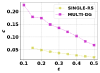
(b) delicious50k $c$

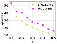
(c) delicious50k queries

(d) delicious50k memory

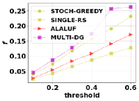
(e) astro $f$

(f) astro $c$

(g) astro queries

(h) astro memory

Figure 3: The experimental results of running the algorithms on instances of diverse data summarization on the delicious (“delicious50k”) dataset, and instances of graph cut on the ca-AstroPh (“astro”) dataset. Multi using the double greedy algorithm of Buchbinder et al. (2015) is referred to as “MULTI-DG”. Single using random sets as described by Feige et al. (2011) is referred to as “SINGLE-RS”. The SC algorithms using the stochastic greedy algorithm of Buchbinder et al. (2017) and the streaming algorithm of Alaluf et al. (2019) are referred to as “STOCH-GREEDY” and “ALALUF” respectively. All $x$ and $y$ axes are normalized as described in Section 4.2.

The experimental results are presented in Figure 3. In every experiment, the double greedy USM algorithm of Buchbinder et al. (2015) (“DG”) is initially run as a baseline comparison. Let the cost, $f$ value, and number of queries of DG be $c_{0}$, $f_{0}$, and $q_{0}$ respectively. For all of the plots, the $f$ values on the y-axis are normalized by $f_{0}$, the $c$ values by $c_{0}$, the number of queries by $q_{0}$, and the max memory by $n$. Notice that the total cost in memory at one time of the algorithm is $n$.

In the first set of experiments, Multi and Single are run on the delicious50k dataset with input $\tau=f_{0}$ and varying $\epsilon$ (Figures 3(a) to 3(d)). In Figure 3(a), one can see that the $f$ values of the solutions returned by each algorithm are close to their theoretical bounds. This is because the guaranteed lower bound on $f$ of $\gamma(1-\epsilon)\tau$ (where $\gamma$ is 1/2 in Multi and 1/4 in Single) is used explicitly in both Multi and Single in order to decide which solutions to choose. In addition, one can see in Figures 3(b) and 3(d) that Multi and Single substantially improve on the baseline DG when it comes to the solution cost $c$, as well as the maximum cost of all elements held in memory at once. On the other hand, Multi and Single make more queries to $f$ compared to DG as demonstrated in Figure 3(c). Single having lower $f$ and $c$ values compared to Multi is a result of the different subroutines used to solve USM; if they used the same one their solutions would be expected to be about the same. This is demonstrated in the experiments in the appendix. As seen in Figure 3(d), Single has higher maximum total cost of all elements held in memory at once than Multi, which is because Single may have instances of Stream corresponding to too high of guesses of $OPT$ as described in Section 3.3. Single makes few queries to $f$ relative to Multi, but this is because it is using a constant time subroutine for USM, if Single used DG it would make significantly more queries to $f$ compared to Multi, as shown in the experiments in the appendix.

In the second set of experiments, Multi and Single are run on the ca-AstroPh dataset with varying input $\tau$ (Figures 3(e) to 3(h)). Figure 3(e) demonstrates that Multi reaches the highest $f$ values, followed by the cover algorithm using the stochastic greedy algorithm of (Buchbinder et al., 2017) (“SG”), then the cover algorithm using the streaming algorithm of Alaluf et al. (2019) (“AL”), and then finally Single. This is the order of their theoretical guarantees on $f$, with the exception of AL and Single being reversed. In addition, the algorithms all perform close to their worst case theoretical guarantees on $f$ as seen in the first set of experiments. Again, both these patterns are to be expected because the algorithms all explicitly choose their solutions based on their lower bound. Heuristic versions of the algorithms where the lower bound is assumed to be the same for all of them are compared in the appendix. In Figure 3(f), one can see that Multi tends to produce a solution of higher cost compared to SG and AL, which is in line with their theoretical guarantees. However, Single produces the lowest cost solution of all despite having the same theoretical bound on cost as Multi. In Figure 3(g), Multi and Single make relatively low total number of queries to $f$. SG is not included in Figure 3(h) since it requires the entire ground set in memory. Figure 3(h) demonstrates that Multi has the lowest maximum total stored cost in memory at once, and despite having the highest Single is reasonably close to the other two.

5 Additional Content to Section 2

In this section, we include a more thorough comparison with the algorithm of Alaluf et al. (2020). Alaluf et al. studied the problem of non-monotone submodular maximization subject to a cardinality constraint $\kappa$, which is the special case of KCSM where the cost $w$ is uniform, in the streaming setting. Their algorithm uses an offline $\alpha$-approximation algorithm for non-monotone submodular maximization as a subroutine, and finds an $\alpha/(1+\alpha)-\epsilon$ approximate solution in a single pass with at most $O(\kappa/\epsilon^{2})$ elements stored at once, and makes at most $O((\log(k)+\log(1+\alpha))/\epsilon^{2})$ queries of $f$. Their algorithm works by making a pass through $U$ and filtering down the ground set, where $O(1/\epsilon)$ disjoint sets are maintained, in a related way to Stream. Finally, they run their $\alpha$-approximation algorithm for cardinality constrained submodular maximization on the union of the disjoint sets. Multi, Single, and SingleMax are different than the algorithm of Alaluf et al. in a number of ways: (1) Multi and Single are for SC, a different optimization problem; (2) Alaluf et al. did not have to deal with the same difficulties as Multi and Single in order to maintain low memory because the cost of the optimal solution is known to be $\kappa$; (3) The final algorithm on the pooled sets for Stream is an algorithm for unconstrained submodular maximization, not cardinality constrained submodular maximization as in Alaluf et al.; (4) Alaluf et al. only considers uniform cost; (5) The conditions Stream uses to store an element is different from what is used by Alaluf et al..

6 Additional Content to Section 3

Proofs and helper lemmas which were omitted from the section Algorithms and Theoretical Guarantees are presented here. In addition, an example of what makes a single pass algorithm difficult to develop for SC is presented. Finally, a more thorough description of the algorithms Single and SingleMax are included.

6.1 Omitted Lemmas and Proofs

The following is Theorem 1, the proof of which was omitted in Section 3. Theorem 1 describes the limitations of how well we can find feasible solutions for SC in polynomial time, and is a clear result from the fact that USM cannot be approximated in polynomial time better than $1/2$ assuming the value query model (Feige et al., 2011).

Theorem 1. For any $\epsilon>0$, there are instances of nonnegative symmetric submodular cover such that there is no (adaptive, possibly randomized) algorithm using fewer than $\Omega(\ln(1+\epsilon)e^{\epsilon^{2}n}/\ln(n))$ queries that always finds a solution of expected $f$ value at least $(1/2+\epsilon)\tau$.

Proof.

Suppose such an algorithm existed, and let it be called $\mathcal{A}$. Then a new algorithm for unconstrained submodular maximization is defined as follows: $\mathcal{A}$ is run on instance $SC(U,f,(1+\epsilon)^{i})$ for every $i\in\mathbb{Z}$ such that $\max_{u\in U}f(\{u\})\leq(1+\epsilon)^{i}\leq n\max_{u\in U}f(\{u\})$, and the solution with the highest value of $f$ is returned. Notice this results in running $\mathcal{A}$ $\ln(n)/\ln(1+\epsilon)$ times. Because $OPT$ is in the above range, there exists some $i$ such that $(1+\epsilon)^{i-1}\leq OPT\leq(1+\epsilon)^{i}$. Once $\mathcal{A}$ is run on $SC(U,f,(1+\epsilon)^{i})$, by assumption it will return $X$ such that $\mathbb{E}[f(X)]\geq(1/2+\epsilon)\tau$. This contradicts the result of Feige et al.. ∎

Lemma 2 relied on Claim 1 in order to proven. Here, we present a proof of Claim 1, but first we will need a result from Feige et al. (2011).

Lemma 3.

(Lemma 2.2 from Feige et al. (2011)) Let $g:2^{U}\to\mathbb{R}_{\geq 0}$ be a non-negative submodular function. Denote by $A(p)$ a random subset of $A$ where each element appears with probability at most $p$ (not necessarily independently). Then $\mathbb{E}[g(A(p))]\geq(1-p)g(\emptyset)$.

Now we can prove Claim 1 using Lemma 3.

Claim 1. Let $A_{1},...,A_{m}\subseteq U$ be disjoint, and $B\subseteq U$. Then there exists $i\in\{1,...,m\}$ such that $f(A_{i}\cup B)\geq(1-1/m)f(B)$.

Proof.

Define $g(X)=f(B\cup X)$. Then $g$ is a non-negative submodular function. Consider choosing $A$ uniformly randomly from the disjoint sets $A_{1},...,A_{m}$. Then any element of $U$ has probability at most $1/m$ of being in $A$. Then

$$\frac{1}{m}\sum_{i=1}^{m}f(B\cup A_{i}) =\frac{1}{m}\sum_{i=1}^{m}g(A_{i})$$

$$=\mathbb{E}[g(A)]$$

$$\overset{(a)}{\geq}\left(1-\frac{1}{m}\right)g(\emptyset)$$

$$=\left(1-\frac{1}{m}\right)f(B)$$

where (a) is a result from Feige et al. (2011) which is stated as Lemma 3 in the appendix. Therefore there must exist some $i\in\{1,...,m\}$ such that $f(A_{i}\cup B)\geq(1-1/m)f(B)$. ∎

6.2 Limitations of Single Pass Algorithms for SC

To see the difficulty with making a single pass through $U$, suppose we have some single pass streaming algorithm for SC that produces a solution with constraint approximation $\beta$. Consider two instances of SC with uniform cost $w$ defined as follows: (i) SC $(\{u_{1},...,u_{n}\},f_{1},w,\tau)$ where $f_{1}$ is modular and $f(u_{i})=\tau/n$ for all $i$; (ii) SC $(\{u_{1},...,u_{n}\},f_{2},w,\tau)$ where $f_{2}$ is modular and $f(u_{i})=\tau/n$ for all $i\neq n$ and $f(u_{n})=\tau$. Suppose the algorithm receives the universe in order $u_{1},...,u_{n}$. Then because the returned solution has constraint value at least $\beta n$, in instance (i) the algorithm must store at least $\beta n-1$ elements before reading element $u_{n}$. On the other hand, instances (i) and (ii) are indistinguishable up to element $u_{n}$, therefore for instance (ii) the algorithm also stores at least $\beta n-1$ elements. However, $OPT=1$ in the latter case, and therefore this stored memory is very large compared to $OPT$.

6.3 The Algorithm Single

Algorithm 3 Single

Input: Value oracles to $f$ and $w$, $\tau$, $\epsilon$, and $B$
Output: $S\subseteq U$

1:  $S[(1+\epsilon)^{i},j]\leftarrow\emptyset$ $\forall i\in\mathbb{Z},j\in\{0,...,2/\epsilon\}$

2:  $L\leftarrow-1$

3:  for $u$ received from stream do

4:     if $f(u)/w(u)>\epsilon\tau/(2L)$ then

5:        $L\leftarrow\epsilon\tau w(u)/(2f(u))$

6:     end if

7:     for $\sigma$ in $\{(1+\epsilon)^{i}:i\in\mathbb{Z},L\leq(1+\epsilon)^{i}\leq B\}$ do

8:        if $w(S[\sigma,i])<2\sigma/\epsilon$ $\forall i$ and $w(u)\leq\sigma$ then

9:           if $\exists i$ s.t. $\Delta f(S[\sigma,i],u)\geq w(u)\epsilon\tau/(2\sigma)$ then

10:              $S[\sigma,i]\leftarrow S[\sigma,i]\cup\{u\}$

11:           end if

12:        end if

13:        $S[\sigma,0]\leftarrow$UnconsMax_γ $(\cup_{i=1}^{2/\epsilon}S_{\sigma,i})$

14:        if $\max\{f(S[\sigma,i]):i\in\{0,...,2/\epsilon\}\}\geq\gamma(1-\epsilon)\tau\}$ then

15:           $B\leftarrow\sigma$

16:        end if

17:     end for

18:  end for

19:  return $\text{argmax}\{f(S[B,i]):i\in\{0,...,2/\epsilon\}\}$

Single works in a similar way to Multi, except: (i) The instances of Stream corresponding to each guess of $OPT$ are running in parallel rather than sequentially; (ii) Instead of each instance of Stream running UnconsMax_γ at the end, UnconsMax_γ is run periodically as elements are received. A lower bound on the guesses of $OPT$, $L$, is updated lazily as Single runs. An upper bound on the guesses of $OPT$, $B$, is initially given as an input and then is updated by running UnconsMax_γ over stored elements periodically as Single runs. Guesses of $OPT$ are $\{(1+\epsilon)^{i}:i\in\mathbb{Z},L\leq(1+\epsilon)^{i}\leq B\}$, and each guess of $OPT$ corresponds to an instance of Stream running in parallel. The sets for the instance of Stream corresponding to guess $\sigma$ are $S[\sigma,0],...,S[\sigma,2/\epsilon]$. In particular, let $U_{i}=\{u_{1},...,u_{i}\}$ be the elements received at a certain point of Stream. Then the lower bound $L$ is $L=\min\{\epsilon\tau w(u)/(2f(u)):u\in U_{i}\}$. $B$ is maintained such that there does not exist a guess $\sigma$ such that $\sigma<B$ and $\max\{f(S[\sigma,i]):i\in 2/\epsilon\}\geq\gamma(1-\epsilon)\tau$, i.e. only the biggest guess of $OPT$ has found a solution with $f$ value at least $\gamma(1-\epsilon)\tau$, if such a solution has been found at all. Any instances of Stream corresponding to guesses of $OPT$ above the upper bound are assumed to be discarded. Pseudocode for Single is given in Algorithm 3.

Theorem 3. Suppose that Single is run for an instance of SC, and input $B\geq OPT$. Define the following two functions:

$$m(x)=(1+\epsilon)(4/\epsilon^{2}+1)\frac{x\ln\left(2x/(\epsilon\tau\xi)\right)}{\ln(1+\epsilon)}$$

$$q(x)=\frac{\ln\left(2x/(\epsilon\tau\xi)\right)}{\ln(1+\epsilon)}\left(\frac{2}{\epsilon}+\frac{\mathcal{T}((4/\epsilon^{2}+1)x)}{w_{min}}\right)$$

where $\xi=\min_{u\in U}w(u)/f(\{u\})$, and $\mathcal{T}(m)$ is the number of queries of UnconsMax_γ on an input set of size $m$. Then, Single:

• Returns a set $S$ such that $f(S)\geq\gamma(1-\epsilon)\tau$ and $w(S)\leq O/PT$;

• The total cost of all elements stored at once is at most $m(B)$;

• Makes at most $q(B)$ queries of $f$ per arriving element of the stream.

Let $u_{1},...,u_{n}$ be the order that the elements of $U$ arrive in, and $U_{i}=\{u_{1},...,u_{i}\}$. If the instance $SC(U_{i},f,w,\tau)$ is feasible and has optimal cost $OPT_{i}$, then from the end of the $i$th iteration of the loop in Single onwards:

• The total cost of all elements stored at once is at most $m(OPT_{i})$;

• At most $q(OPT_{i})$ queries of $f$ are made per arriving element of the stream.

Proof.

Consider an alternate version of Stream where instead of running UnconsMax_γ on $\cup S_{i}$ after receiving all elements in the stream (Line 10), UnconsMax_γ is run at the end of each iteration of the loop on Line 2 of Stream. Notice that this does not change any of the properties of Stream detailed in Lemmas 1 and 2 except the number of queries to $f$. From this point on in the proof, we will consider this alternative version of Stream.

Consider the value of $B$ at the end of some iteration of the for loop on Line 3 of Single. It is now shown that without loss of generality, one can assume that up to this point Single is running Stream in parallel with guesses of $OPT$ $\{(1+\epsilon)^{i}:i\in\mathbb{Z},(1+\epsilon)^{i}\leq B\}$. $B$ is only decreasing throughout Stream, and so changes in $B$ only result in removing instances of Stream, not adding them. Therefore we only need to show that guesses of $OPT$ smaller than $B$ are w.l.o.g. running in parallel.

Consider any $(1+\epsilon)^{i}\leq B$. Consider any previous iteration of the loop on Line 3 such that for the first time an $u$ has arrived such that $\Delta f(\emptyset,u)\geq w(u)\epsilon\tau/(2(1+\epsilon)^{i})$ (i.e. the first time an element should be added to $S[(1+\epsilon)^{i},j]$ for some $j\in\{1,...,2/\epsilon\}$), and we are at the beginning of the loop on Line 3. If $L>(1+\epsilon)^{i}$, then

$$f(u)/w(u) \geq\Delta f(\emptyset,u)/w(u)$$

$$\geq\epsilon\tau/(2(1+\epsilon)^{i})$$

$$>\epsilon\tau/(2L).$$

Therefore the if statement on Line 4 will be true, $L$ will be reset to $\epsilon\tau w(u)/(2f(u))$, and $(1+\epsilon)^{i}$ added to the guesses of $OPT$ since

$$(1+\epsilon)^{i} \geq w(u)\epsilon\tau/(2\Delta f(\emptyset,x))$$

$$\geq L.$$

Item (i) is now proven. By Lemma 2, if there exists a run of Stream with a guess of $OPT$ that is at least as big, then the set returned by Stream has $f$ value at least $\gamma(1-\epsilon)\tau$. Therefore by the end of Single, any run of Stream corresponding to a guess of $OPT$ that is at least as big as $OPT$ must have triggered the if statement on Line 14. Initially $B\geq OPT$, and only decreases if the if statement on Line 14 is true, it must be that the solution $S$ of Single has $f(S)\geq\gamma(1-\epsilon)\tau$. In addition, the above discussion implies that $B$ is no greater than $(1+\epsilon)OPT$ at the end of Single, then Lemma 1 implies the remaining part of item (i).

Item (ii) is now proven. By Lemma 1, the total cost of all elements stored by each run of Stream with input $(\epsilon,\sigma)$ is $(4/\epsilon^{2}+1)\sigma$, which is bounded above by $(4/\epsilon^{2}+1)B$. In addition, $L\geq\epsilon\tau\xi/2$, and therefore there are at most $\ln(2B/(\epsilon\tau\xi))/\ln(1+\epsilon)$ parallel instances of Stream running in Single. This proves item (iii).

Item (iii) is now proven. Since $B$ is the biggest guess of $OPT$, the alternative versions of Stream that Single is running makes at most $2/\epsilon+\mathcal{T}((4/\epsilon^{2}+1)\overline{OPT}/w_{min})\leq 2/\epsilon+\mathcal{T}((4/\epsilon^{2}+1)B/w_{min})$ queries to $f$ per element, which can be proven using the same argument as in Lemma 1. Combining this with the fact that there are at most $\ln(2B/(\epsilon\tau\xi))/\ln(1+\epsilon)$ parallel instances of Stream running proves item (iii).

Finally, item (iv) and (v) are proven. Suppose the iteration of the for loop on Line 3 corresponding to element $u_{i}$ is complete. By a nearly identical argument to that used for item (i), one can see that the largest guess of $OPT$ is no bigger than $(1+\epsilon)OPT_{i}$ from this point on. Therefore the largest memory for any run of Stream from this point on is $O/PT_{i}$, and any run will make at most $2/\epsilon+\mathcal{T}((4/\epsilon^{2}+1)OPT_{i}/w_{min})$ queries per element received, which can be proven using the same argument as in Lemma 1. There are at most $\ln(2OPT_{i}/(\epsilon\tau\xi))$ parallel instances of Stream running in Single. Altogether this implies items (iv) and (v).

∎

6.3.1 The Algorithm SingleMax

The algorithm SingleMax was presented for the problem KCSM in Section 3.4. In KCSM, the $f$ value of the optimal solution is unknown (in contrast, in SC it is known to be $\tau$). KCSM runs versions of Stream in parallel where instead of input $\overline{OPT}$, $\overline{OPT}$ is fixed at $\kappa$, and instead the value of $\tau$ is guessed. In particular, the set $\{(1+\epsilon)^{i}:i\in\mathbb{Z},m\leq(1+\epsilon)^{i}\leq 2m\kappa/\epsilon\}$ are the guesses of $OPT$ Because the cost of the optimal solution is known to be at most $\kappa$ in KCSM, the total stored cost at once for every instance of Stream is bounded by $(4/\epsilon^{2}+1)\kappa$ (see Lemma 1). For this reason, we avoid difficulties of having too high total stored cost as we did in Single. SingleMax lazily keeps track of an upper and lower bound for the $f$ value of the optimal solution as elements arrive from the stream in a similar manner as the lower bound $L$ was updated in Single. Pseudocode for SingleMax is presented in Algorithm 4. In addition, the theoretical guarantees of SingleMax, stated in Theorem 4 of the main content, are proven below.

Algorithm 4 SingleMax

Input: Value oracles to $f$ and $w$, $\kappa$, and $\epsilon$
Output: $S\subseteq U$

1:  $S[(1+\epsilon)^{i},j]\leftarrow\emptyset$ $\forall i\in\mathbb{Z},j\in\{0,...,2/\epsilon\}$

2:  for $x$ received from stream do

3:     if $f(\{x\})/w(x)>m$ then

4:        $m\leftarrow f(\{x\})/w(x)$

5:     end if

6:     for $\tau$ in $\{(1+\epsilon)^{i}:i\in\mathbb{Z},m\leq(1+\epsilon)^{i}\leq 2m\kappa/\epsilon\}$ do

7:        if $w(S[\tau,i])<2\kappa/\epsilon$ $\forall i$ and $w(x)\leq\kappa$ then

8:           if $\exists i$ s.t. $\Delta f(S[\tau,i],x)\geq w(x)\epsilon\tau/(2\kappa)$ then

9:              $S[\tau,i]\leftarrow S[\tau,i]\cup\{x\}$

10:           end if

11:        end if

12:     end for

13:  end for

14:  for $\tau$ in $T$ do

15:     $S[\tau,0]\leftarrow$UnconsMax_γ $(\cup_{i=1}^{2/\epsilon}S[\tau,i])$

16:  end for

17:  return $\text{argmax}\{f(S[\tau,i]):\tau\in T,i\in\{0,...,2/\epsilon\}\}$

Theorem 4. Suppose that SingleMax is run for an instance of KCSM: Then:

• The set $S$ returned by SingleMax satisfies $f(S)\geq\gamma(1-\epsilon)OPT$ and $w(S)\leq\kappa/$;

• The total cost of all elements needing to be stored at once is at most $(4/\epsilon^{2}+1)\ln(2\kappa/(w_{min}\epsilon))/\ln(1+\epsilon)\kappa$;

• And at most $\ln(2\kappa/(w_{min}\epsilon))(2n/\epsilon+\mathcal{T}((4/\epsilon^{2}+1)\kappa))/\ln(1+\epsilon)$ queries of $f$ are made in total where $\mathcal{T}(m)$ is the number of queries of UnconsMax_γ on an input set of size $m$.

Proof.

In order to prove Theorem 4, a new version of Lemma 2 is needed. The following Lemma is proved in as essentially identical way to Lemma 2:

Lemma 4.

Suppose that Stream is run with input $\epsilon\in(0,1)$, and $\tau\geq OPT$. Let $S$ be the set returned by Stream. Then $f(S)\geq\gamma(1-\epsilon)OPT$.

Similar to Single, SingleMax is essentially running a bunch of instances of Stream in parallel as $U$ is read in. In particular, the set $\{(1+\epsilon)^{i}:i\in\mathbb{Z},m\leq(1+\epsilon)^{i}\leq 2m\kappa/\epsilon\}$ are the guesses of $OPT$, and there is an instance of Stream corresponding to each guess. For each guess $\tau$, $S_{\tau,0},...,S_{\tau,2/\epsilon}$ in Single correspond to the sets $S_{0},...,S_{2/\epsilon}$ in Stream.

Define $q\in\mathbb{Z}$ to be the unique value such that

$$(1+\epsilon)^{q}\leq OPT<(1+\epsilon)^{q+1}.$$

Then we may assume without loss of generality that there is an instance of Stream corresponding to $(1+\epsilon)^{q}$ as a guess of $OPT$ for the duration of SingleMax, as explained as follows. First of all, clearly $(1+\epsilon)^{q}\geq\max\{f(\{x\}):x\in U\}$ and therefore is at least the smallest guess throughout the duration of SingleMax. On the other hand, suppose that for the first time we have received from the stream an element $x$ such that $\Delta f(\emptyset,x)\geq\epsilon w(x)(1+\epsilon)^{q}/(2\kappa)$ (i.e. the first time an element $x$ should be added to $S_{(1+\epsilon)^{q},i}$ for some $i\in\{1,...,2/\epsilon\}$). If $(1+\epsilon)^{q}>2m\kappa/\epsilon$ at the beginning of the for loop then

$$f(\{x\})/w(x) \overset{(a)}{\geq}\Delta f(\emptyset,x)/w(x)$$

$$\geq\epsilon(1+\epsilon)^{q}/(2\kappa)$$

$$>m$$

where (a) is because $f(\emptyset)\geq 0$. Therefore the if statement will be true, $m$ will be re-assigned as $f(\{x\})/w(x)$, and $(1+\epsilon)^{q}$ added to the guess of $OPT$ since

$$(1+\epsilon)^{q} \leq 2\Delta f(\emptyset,x)\kappa/(w(x)\epsilon)$$

$$\leq 2f(\{x\})\kappa/(w(x)\epsilon)$$

$$=2m\kappa/\epsilon$$

and will remain in the guesses until the end.

In light of the above, items (i), (ii), and (iii) follow by an analogous argument as in Theorem 3. ∎

7 Additional Content to Section 4

The experimental results here are a superset of those included in the main paper. In addition, additional details about the applications and setup are included here.

7.1 Applications of SC

In sections 4, the algorithms Single and Multi are evaluated on instances of non-monotone submodular cover involving graph cut (Balkanski et al., 2018) and diverse summarization (Tschiatschek et al., 2014) functions. Definitions of both of these applications are now provided.

The first application considered is SC where $f$ is a graph cut function, which is a submodular but not necessarily monotone function. Graph cut functions have frequently been used as applications of non-monotone submodular maximization. A graph cut function takes in a set of vertices in a graph $X$ and computes the total number of edges between $X$ and $U\setminus X$. The problem definition is defined as follows.

Definition 1 (Graph cut).

Let $G=(V,E)$ be a graph, and $w:E\to\mathbb{R}_{\geq 0}$ be a function that gives a weight for every edge in the graph. Define $f:2^{U}\to\mathbb{R}_{\geq 0}$ to be a function that takes $X\subseteq V$ to the total weight of edges between $X$ and $V\setminus X$, i.e.

$$f(X)=\sum_{x\in X,y\notin X}w(x,y).$$

Then $f$ is submodular and non-negative, but is not necessarily monotone.

The second application considered is SC where $f$ is a diverse data summarization function, which is also a submodular but not necessarily monotone function. A diverse data summarization function takes in a subset $X$ of a data set $U$ and returns a score of how effective $X$ summarizes $U$, while penalizing for similarity between the elements of $X$. Variants of diverse data summarization are also a popular application for non-monotone submodular maximization. The particular formulation used here is based on tagged data, and is defined as follows.

Definition 2 (Diverse summarization of a tagged data set).

Suppose the data points in $U$ are each tagged by a subset of tags $T$ via the function $t:U\to 2^{T}$. E.g. if $U$ is a set of images then $T$ may be words describing each image. Given parameter $\gamma\geq 0$, define $f:2^{U}\to\mathbb{R}_{\geq 0}$ to be

$$f(X)=|\cup_{x\in X}t(X)|-\gamma\sum_{x\in X,y\in X}\frac{|t(x)\cup t(y)|}{|t(x)\cap t(y)|}.$$

The first term in $f(X)$ is the total number of tags covered by a summary $X$, while the second term is a penalty to encourage diversity in the summary (using the Jaccard similarity). $f$ is submodular, but not necessarily monotone or non-negative. If $\gamma$ is sufficiently small, then $f$ is non-negative.

For the experiments in this paper, we set

$$\gamma=|\cup_{x\in U}t(X)|/\sum_{x\in U,y\in U}\frac{|t(x)\cup t(y)|}{|t(x)\cap t(y)|}.$$

7.2 Experimental Setup

The graph cut instances presented here are on the ca-AstroPh ($n=18772$, 198110 edges), com-Amazon ($n=334863$, 925872 edges), and email-Enron ($n=36692$, 183831 edges) networks from the SNAP large network collection (Leskovec and Krevl, 2014). In all of the cut instances the cost of each element is uniformly set as 1. The diverse summarization instances are on the Corel5k set of images (Duygulu et al., 2002) ($n=5000$), and a subset of tagged webpages from the delicious.com website (Soleimani and Miller, 2016) ($n=5000$ or $n=50000$ depending on the instance) The smaller instances are used in some experiments because some the comparison algorithms cannot run on the larger datasets within a couple of hours. Specifically, when the local search algorithm of Feige et al. (2011) is used as a subroutine for USM then Single takes too long to run. In addition, the cover algorithm by using the stochastic greedy algorithm of Buchbinder et al. (2017) for submodular maximization along with the approach of Iyer and Bilmes (2013) takes too long to run. The Corel5k images are each losslessly compressed, and their cost is assigned to be their size in kB after compression. The costs of the websites from the delicious.com website are uniform.

Several USM algorithms are run as subroutines of Single and Multi: (i) Repeated runs of the randomized double greedy algorithm of Buchbinder et al. (2015) (“DG”); (ii) The local search algorithm of Feige et al. (2011) with parameter 0.25 (“LS”), which is a deterministic $1/3$ approximation for USM, and on a set of size $r$ makes $O(r^{3}\ln(r))$ queries to $f$; (iii) Repeatedly returning a random set, as described by Feige et al. (2011) (“RS”). The randomized algorithms for USM (i and iii) are repeated 50 times and the best solution is chosen.

The comparison algorithms using the method of Iyer and Bilmes (2013) described in the main text are only for uniform cost. For the Corel5k dataset, which has non-uniform cost, we use a modified version of each algorithm where the marginal gain function $\Delta f(X,x)$ is replaced by $\Delta f(X,x)/w(x)$. This modified version does not have any proven approximation guarantee.

7.3 Additional Experimental Results

The additional experimental results are presented in Figures 4 to 8. In every experiment, the double greedy USM algorithm of Buchbinder et al. (2015) (“DG”) is initially run as a baseline comparison. Let the cost, $f$ value, and number of queries of DG be $c_{0}$, $f_{0}$, and $q_{0}$ respectively. For all of the plots, the $f$ values on the y-axis are normalized by $f_{0}$, the $c$ values by $c_{0}$, the threshold $\tau$ by $f_{0}$, the number of queries by $q_{0}$, and the max memory by $n$. Notice that the total cost in memory at one time of the algorithm is $n$.

The first set of experiments compare different USM algorithms used as a subroutine in Stream. The results for Multi are in Figure 4, and the results for Single are in Figure 5. One can see that no matter the algorithm used for USM, Multi and Single can substantially improve on the unconstrained algorithm DG when it comes to cost ($c$) while reaching reasonably high values of $f$. As observed in Section 4 in the main paper, The $f$ values of the solutions returned are close to their theoretical bounds. When DG is the subroutine for USM then the highest $f$ value is returned, and RS returns the lowest $f$ value, as expected based on their approximation guarantees. Surprisingly, for Multi the DG subroutine results in the highest total number of queries to $f$ despite LS being the algorithm with the highest theoretical run time. This is because Multi is making a lot more passes to reach the higher approximation guarantee of DG relative to LS. This results in more total queries to $f$ since each pass is $O(n/\epsilon)$ queries even before any USM subroutine is used. Any of the subroutines are practical for Multi in terms of number of queries. In all other experiments, we set DG as the subroutine for Multi since it gives the highest $f$ value. In contrast, both DG and LS are relatively impractical in terms of the number of queries for Single since Single needs to run USM so many times, especially as $\epsilon$ decreases. Therefore in all other experiments we use RS as the subroutine for Single.

In the second set of experiments, Multi and Single are run on the instances of diverse data summarization on the Corel5k (“corel”) and delicious (“delicious50k”) dataset with $n=50000$, and instances of graph cut on the ca-AstroPh (“astro”) and com-Amazon (“amazon”) datasets. with input $\tau=f_{0}$ and varying $\epsilon$ (Figure 6). These experiments are just like those in Figures 3(a) to 3(d) of the main paper, and are presented here to show that the same patterns hold for additional datasets. Similarly, in Figure 7, Multi and Single are run with varying input $\tau$ and the results are similar to those featured in Figures 3(e) to 3(h) in the main paper.

Finally, in Figure 8 the same experiments as in Figure 7 are run except the algorithms are run as heuristics where the approximation guarantees are assumed to be 1. In particular, Multi and Single both run Stream where $\gamma=1$, and when the approach of Iyer and Bilmes (2013) is used the submodular maximization subroutines are run until a solution is found with $f$ value at least $(1-\epsilon)\tau$. The purpose of these experiments is to compare the algorithms without explicitly using their known approximation guarantees, since that was found to heavily influence the $f$ values of the solutions in Figure 7 as discussed in the main text. The differences in $f$ values between the algorithms are now practically eliminated, and the difference in cost values greatly lessened although ALALUF and SG still find relatively lower cost solutions. However, the differences in memory and queries to $f$ between the algorithms are increased. This is because the approach of Iyer and Bilmes (2013) requires running ALALUF and SG many more times to reach the higher threshold for $f$. In this setting, ALALUF and SG are not practical because of their large numbers of queries compared to Multi and Single.

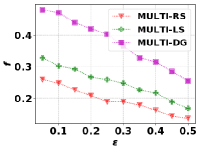
(a) enron, cut

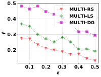
(b) astro, cut

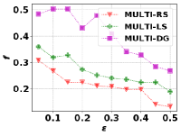
(c) corel, cover

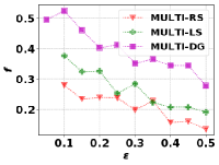
(d) delicious5k, cover

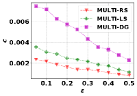
(e) enron, cut

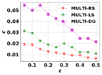
(f) astro, cut

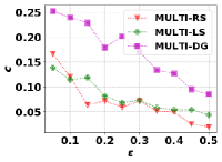
(g) corel, cover

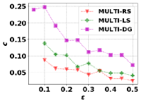
(h) delicious5k, cover

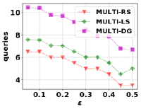
(i) enron, cut

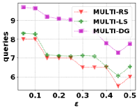
(j) astro, cut

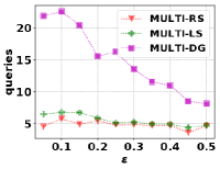
(k) corel, cover

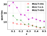
(l) delicious5k, cover

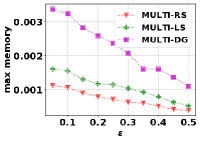
(m) enron, cut

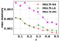
(n) astro, cut

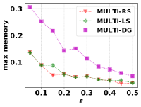
(o) corel, cover

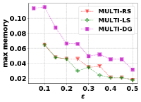
(p) delicious5k, cover

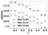
(q) enron, cut

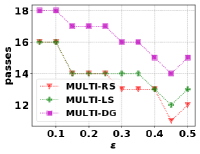
(r) astro, cut

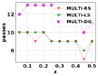
(s) corel, cover

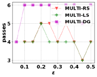
(t) delicious5k, cover

Figure 4: A comparison of the performance of Multi using different algorithms for USM as a subroutine. $f$ and $c$ refer to the $f$ and cost values of the returned solution. Queries is the total number of queries to $f$ that the algorithm took. Max memory is the maximum cost of all elements stored at once over the duration of the algorithm. The instances of graph cut and diverse data summarization are on the Corel5k (“corel”) and delicious (“delicious5k”) dataset, and instances of graph cut are on the ca-AstroPh (“astro”) and email-Enron (“amazon”) datasets. Multi using the double greedy algorithm of Buchbinder et al. (2015), the local search algorithm of Feige et al. (2011), and the random set algorithm are referred to as “MULTI-DG”, “MULTI-LS”, and “MULTI-RS” respectively. All $x$ and $y$ axes are normalized as described in Section 7.3.

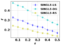
(a) enron, cut

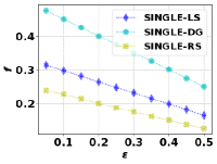
(b) astro, cut

(c) corel, cover

(d) delicious5k, cover

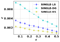
(e) enron, cut

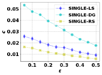
(f) astro, cut

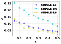
(g) corel, cover

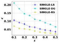
(h) delicious5k, cover

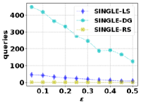
(i) enron, cut

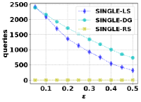
(j) astro, cut

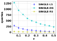
(k) corel, cover

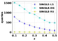
(l) delicious5k, cover

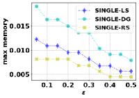
(m) enron, cut

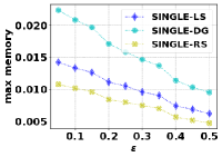
(n) astro, cut

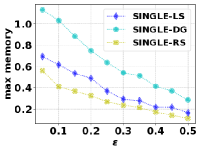
(o) corel, cover

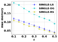
(p) delicious5k, cover

Figure 5: A comparison of the performance of Single using different algorithms for USM as a subroutine. Single using the double greedy algorithm of Buchbinder et al. (2015), the local search algorithm of Feige et al. (2011), and the random set algorithm are referred to as “SINGLE-DG”, “SINGLE-LS”, and “SINGLE-RS” respectively.

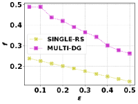
(a) amazon, cut

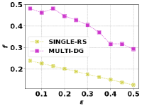
(b) astro, cut

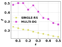
(c) corel, cover

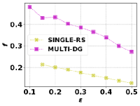
(d) delicious50k, cover

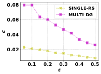
(e) amazon, cut

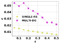
(f) astro, cut

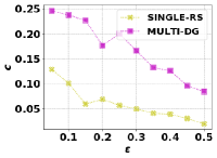
(g) corel, cover

(h) delicious50k, cover

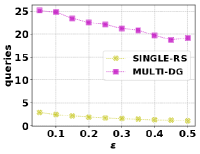
(i) amazon, cut

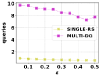
(j) astro, cut

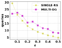
(k) corel, cover

(l) delicious50k, cover

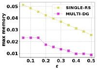
(m) amazon, cut

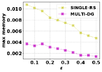
(n) astro, cut

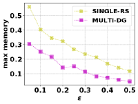
(o) corel, cover

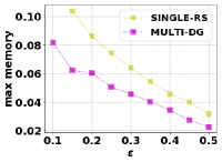
(p) delicious50k, cover

Figure 6: The outcome of running Multi and Single for varying $\epsilon$ on instances of diverse data summarization on the Corel5k (“corel”) and delicious (“delicious50k”) dataset with $n=50000$, and instances of graph cut on the ca-AstroPh (“astro”) and com-Amazon (“amazon”) datasets.

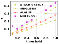
(a) enron, cut

(b) astro, cut

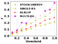
(c) corel, cover

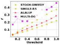
(d) delicious, cover

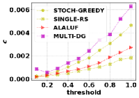
(e) enron, cut

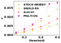
(f) astro, cut

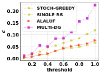
(g) corel, cover

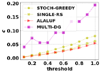
(h) delicious, cover

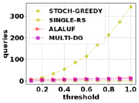
(i) enron, cut

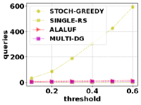
(j) astro, cut

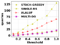
(k) corel, cover

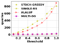
(l) delicious, cover

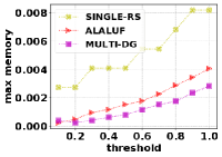
(m) enron, cut

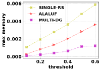
(n) astro, cut

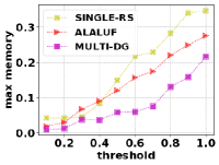
(o) corel, cover

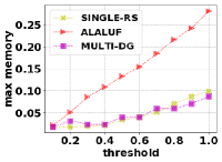
(p) delicious, cover

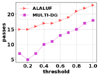
(q) enron, cut

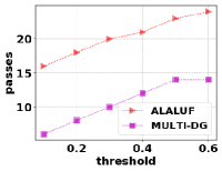
(r) astro, cut

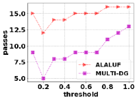
(s) corel, cover

(t) delicious, cover

Figure 7: A comparison of algorithms for SC using different thresholds $\tau$ (normalized as described in Section 7.3). STOCH-GREEDY is converting the stochastic greedy algorithm of Buchbinder et al. (2017) to an algorithm for SC by using the method of Iyer and Bilmes (2013). ALALUF is the same, but using the algorithm of Alaluf et al. (2019).

(a) enron, cut

(b) astro, cut

(c) corel, cover

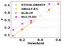
(d) delicious, cover

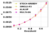
(e) enron, cut

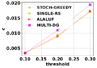
(f) astro, cut

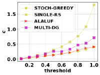
(g) corel, cover

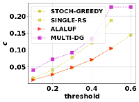
(h) delicious, cover

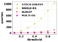
(i) enron, cut

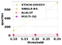
(j) astro, cut

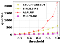
(k) corel, cover

(l) delicious, cover

(m) enron, cut

(n) astro, cut

(o) corel, cover

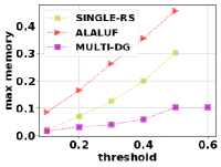
(p) delicious, cover

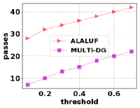
(q) enron, cut

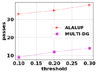
(r) astro, cut

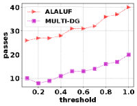
(s) corel, cover

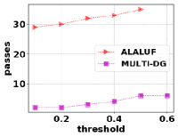
(t) delicious, cover

Figure 8: A comparison of algorithms for SC using different thresholds $\tau$. However, the algorithms are run as heuristics where all approximation guarantees are assumed to be 1. See Section 7.3 to see further description.

References

- Alaluf et al. (2019) N. Alaluf, A. Ene, M. Feldman, H. L. Nguyen, and A. Suh. Optimal streaming algorithms for submodular maximization with cardinality constraints. arXiv preprint arXiv:1911.12959, 2019.
- Alaluf et al. (2020) N. Alaluf, A. Ene, M. Feldman, H. L. Nguyen, and A. Suh. Optimal streaming algorithms for submodular maximization with cardinality constraints. In 47th International Colloquium on Automata, Languages, and Programming (ICALP 2020). Schloss Dagstuhl-Leibniz-Zentrum für Informatik, 2020.
- Balkanski et al. (2018) E. Balkanski, A. Breuer, and Y. Singer. Non-monotone submodular maximization in exponentially fewer iterations. Advances in Neural Information Processing Systems, 31, 2018.
- Buchbinder and Feldman (2016) N. Buchbinder and M. Feldman. Constrained submodular maximization via a non-symmetric technique. arXiv preprint arXiv:1611.03253v1, 2016.
- Buchbinder and Feldman (2018a) N. Buchbinder and M. Feldman. Deterministic Algorithms for Submodular Maximization. ACM Transactions on Algorithms, 14(3), 2018a.
- Buchbinder and Feldman (2018b) N. Buchbinder and M. Feldman. Deterministic algorithms for submodular maximization problems. ACM Transactions on Algorithms (TALG), 14(3):1–20, 2018b.
- Buchbinder et al. (2014) N. Buchbinder, M. Feldman, J. Naor, and R. Schwartz. Submodular maximization with cardinality constraints. In Proceedings of the twenty-fifth annual ACM-SIAM symposium on Discrete algorithms, pages 1433–1452. SIAM, 2014.
- Buchbinder et al. (2015) N. Buchbinder, M. Feldman, J. Seffi, and R. Schwartz. A tight linear time (1/2)-approximation for unconstrained submodular maximization. SIAM Journal on Computing, 44(5):1384–1402, 2015.
- Buchbinder et al. (2017) N. Buchbinder, M. Feldman, and R. Schwartz. Comparing apples and oranges: Query trade-off in submodular maximization. Mathematics of Operations Research, 42(2):308–329, 2017.
- Chakrabarti and Kale (2015) A. Chakrabarti and S. Kale. Submodular maximization meets streaming: Matchings, matroids, and more. Mathematical Programming, 154(1):225–247, 2015.
- Crawford et al. (2019) V. Crawford, A. Kuhnle, and M. Thai. Submodular cost submodular cover with an approximate oracle. In International Conference on Machine Learning, pages 1426–1435, 2019.
- Das and Kempe (2018) A. Das and D. Kempe. Approximate submodularity and its applications: Subset selection, sparse approximation and dictionary selection. The Journal of Machine Learning Research, 19(1):74–107, 2018.
- Duygulu et al. (2002) P. Duygulu, K. Barnard, J. F. de Freitas, and D. A. Forsyth. Object recognition as machine translation: Learning a lexicon for a fixed image vocabulary. In European conference on computer vision, pages 97–112. Springer, 2002.
- Feige et al. (2011) U. Feige, V. S. Mirrokni, and J. Vondrák. Maximizing non-monotone submodular functions. SIAM Journal on Computing, 40(4):1133–1153, 2011.
- Gharan and Vondrák (2011) S. O. Gharan and J. Vondrák. Submodular maximization by simulated annealing. In Proceedings of the twenty-second annual ACM-SIAM symposium on Discrete Algorithms, pages 1098–1116. SIAM, 2011.
- Gillenwater et al. (2012) J. Gillenwater, A. Kulesza, and B. Taskar. Near-optimal map inference for determinantal point processes. Advances in Neural Information Processing Systems, 25, 2012.
- Gupta et al. (2010) A. Gupta, A. Roth, G. Schoenebeck, and K. Talwar. Constrained non-monotone submodular maximization: Offline and secretary algorithms. In International Workshop on Internet and Network Economics, pages 246–257. Springer, 2010.
- Hartline et al. (2008) J. Hartline, V. Mirrokni, and M. Sundararajan. Optimal marketing strategies over social networks. In Proceedings of the 17th international conference on World Wide Web, pages 189–198, 2008.
- Iyer and Bilmes (2013) R. K. Iyer and J. A. Bilmes. Submodular optimization with submodular cover and submodular knapsack constraints. In Advances in Neural Information Processing Systems, pages 2436–2444, 2013.
- Kempe et al. (2003) D. Kempe, J. Kleinberg, and É. Tardos. Maximizing the spread of influence through a social network. In Proceedings of the ninth ACM SIGKDD international conference on Knowledge discovery and data mining, pages 137–146. ACM, 2003.
- Leskovec and Krevl (2014) J. Leskovec and A. Krevl. SNAP Datasets: Stanford large network dataset collection. http://snap.stanford.edu/data, June 2014.
- Mirzasoleiman et al. (2015) B. Mirzasoleiman, A. Karbasi, A. Badanidiyuru, and A. Krause. Distributed submodular cover: Succinctly summarizing massive data. In Advances in Neural Information Processing Systems, pages 2881–2889, 2015.
- Mirzasoleiman et al. (2016) B. Mirzasoleiman, M. Zadimoghaddam, and A. Karbasi. Fast distributed submodular cover: Public-private data summarization. In Advances in Neural Information Processing Systems, pages 3594–3602, 2016.
- Nemhauser et al. (1978) G. L. Nemhauser, L. A. Wolsey, and M. L. Fisher. An analysis of approximations for maximizing submodular set functions—i. Mathematical programming, 14(1):265–294, 1978.
- Norouzi-Fard et al. (2016) A. Norouzi-Fard, A. Bazzi, M. El Halabi, I. Bogunovic, Y.-P. Hsieh, and V. Cevher. An efficient streaming algorithm for the submodular cover problem. In Proceedings of the 30th International Conference on Neural Information Processing Systems, pages 4500–4508, 2016.
- Soleimani and Miller (2016) H. Soleimani and D. J. Miller. Semi-supervised multi-label topic models for document classification and sentence labeling. In Proceedings of the 25th ACM international on conference on information and knowledge management, pages 105–114, 2016.
- Tschiatschek et al. (2014) S. Tschiatschek, R. K. Iyer, H. Wei, and J. A. Bilmes. Learning mixtures of submodular functions for image collection summarization. Advances in neural information processing systems, 27, 2014.
- Wan et al. (2010) P.-J. Wan, D.-Z. Du, P. Pardalos, and W. Wu. Greedy approximations for minimum submodular cover with submodular cost. Computational Optimization and Applications, 45(2):463–474, 2010.
- Wolsey (1982) L. A. Wolsey. An analysis of the greedy algorithm for the submodular set covering problem. Combinatorica, 2(4):385–393, 1982.