Determinantal Born-Infeld Coupling of Gravity and Electromagnetism

Abstract

We study a Born-Infeld inspired model of gravity and electromagnetism in which both types of fields are treated on an equal footing via a determinantal approach in a metric-affine formulation. Though this formulation is a priori in conflict with the postulates of metric theories of gravity, we find that the resulting equations can also be obtained from an action combining the Einstein-Hilbert action with a minimally coupled nonlinear electrodynamics. As an example, the dynamics is solved for the charged static black hole.

I Introduction

The study of alternative theories of gravity and matter that may allow to provide a more satisfactory description of Nature has experienced a boost in the last two decades or so, though several examples have been known from much earlier. An important such example is the Born-Infeld theory of electrodynamics [1], in which the Maxwell Lagrangian is classically modified to bound the electric field intensity, so curing the electron self-energy problem of classical electrodynamics. Boosted by the seminal work by Fradkin and Tseytlin [2], determinantal actions also found relevant applications in M-theory scenarios to describe charged D-branes. Following the philosophy of the Born-Infeld electromagnetic theory, attempts to improve the gravitational dynamics at high curvatures have also made Born-Infeld inspired proposals very attractive in more recent years. In particular, Deser and Gibbons [3] considered a theory based on the determinant of the sum of the space-time metric plus the Ricci tensor, but it turned out to be plagued by ghost-like instabilities. A reformulation of this theory in the metric-affine framework was then proposed by Vollick [4], showing that the ghosts are removed. This new model was popularized by Bañados and Ferreira [5], who found that it could also help avoid cosmological singularities. Numerous applications in cosmology, astrophysics, and many other scenarios followed those works, and the reader is referred to the review article [6] for a detailed account of the related literature.

The majority of the Born-Infeld inspired modifications of gravitational theories tend to include the matter following the standard minimal coupling prescription of metric theories of gravity (MTGs) [7], which is a practical rule to make the theory compatible with the Einstein equivalence principle [8]. This rule simply splits the total action into a gravitational part plus a matter part, $S_{Total}=S_{Gravity}+S_{Matter}$, the latter being constructed from the Minkowskian theory by promoting the flat metric $\eta_{\mu\nu}$ to a curved space-time metric $g_{\mu\nu}$, using the language of differential geometry and some minimal coupling prescription (which is not always free of ambiguities [9]), i.e., $S_{Matter}=S[g_{\mu\nu},\Psi_{m},\nabla\Psi_{m}]$, with $\Psi_{m}$ generically representing the matter fields.

Perhaps for this reason, attempts to improve simultaneously the matter and gravitational sectors by combining both in a single determinantal-type action have only received timid attention, with the notable exception, to our knowledge, of the models considered by Vollick in [10], who proposed an action of the form

$$I\propto\int dx^{4}\left[\sqrt{-\det\left(g_{\mu\nu}+\epsilon{R_{\mu\nu}}(\Gamma)+\beta M_{\mu\nu}\right)}-\lambda\sqrt{-g}\right]\ ,$$ (1)

where $M_{\mu\nu}$ represents a quantity constructed with the matter fields, $\epsilon$ and $\beta$ are suitable coupling constants, and $\lambda$ determines the asymptotic behaviour of the vacuum solutions, with $\lambda=1$ yielding Minkowski space-time. For (massless) scalar fields one can take $M_{\mu\nu}=\partial_{\mu}\phi\partial_{\nu}\phi$, for electromagnetic fields $M_{\mu\nu}=F_{\mu\nu}$, and so on. As pointed out above, such a construction does not fit within the gravitational plus matter splitting of metric theories of gravity and this suggests that theories of that type should be at some point in conflict with the experimental evidence supporting the equivalence principle. Nonetheless, Vollick showed that for $M_{\mu\nu}=\partial_{\mu}\phi\partial_{\nu}\phi$ the theory field equations boil down to those of General Relativity (GR) minimally coupled to a free scalar field. For electromagnetic and fermionic fields, at leading order in perturbations, one can see that the usual Einstein-Maxwell and Einstein-Dirac systems are recovered, which shows that such theories admit an MTG representation at that order. This motivates us to go beyond the perturbative analysis of [10] and try to find a complete representation of the field equations of those theories. Due to the technicalities involved, in this paper we will concentrate on the electromagnetic case, for which an exact representation will be provided. We would like to point out that the gravitational-electromagnetic determinantal action has the appealing property that it combines linearly the first derivatives of the affine connection with the first derivatives of the $U(1)$ electromagnetic connection. Thus, in some sense, it is treating in a similar footing spin 1 and spin 2 massless bosons. Understanding the resulting non-perturbative dynamics of such a theory is thus a nontrivial question that deserves genuine attention.

In this work we will show that for the gravitational-electromagnetic case it is possible to find an explicit representation of the full field equations, and that they turn out to admit a reformulation that fits within the family of metric theories of gravity, breaking in this way the apparent conflict posed by the initial representation of the theory. In fact, the gravitational-electromagnetic case turns out to be equivalent, at all orders, to Einstein’s gravity coupled to a nonlinear electrodynamics (NED) theory which, up to a sign, coincides with the Born-Infeld theory. Our results suggest that there might be alternative ways of consistently coupling matter and gravity which break the standard paradigm set by MTGs.

The paper is organized as follows. In Section II we set the determinantal Born-Infeld-like Lagrangian describing the gravitational-electromagnetic system, and display the dynamics resulting in the metric-affine (à la Palatini) formalism. We show that the affine connection turns out to be the Levi-Civita connection. Once the connection has been solved, one can proceed in two ways. On the one hand one can take advantage of the experience gained with Born-infeld-like Lagrangians to get the dynamics in a few steps, as done in Section III. However, this procedure leads to dynamical equations where gravity and electromagnetism are very intermingled. On the other hand, one can rework the dynamics to prove that, in spite of the appearances, the system evolves exactly as expected in an MTG theory, as shown in Section IV. In Section V we solve the dynamics for a charged static black hole to illustrate aspects of the general behaviour. In Section VI we display the conclusions.

II Model and equations

The theory we will be dealing with can be written in compact form as

$$I\propto\int dx^{4}\left[\sqrt{-q}-\lambda\sqrt{-g}\right]$$ (2)

where $g$ is the determinant of the space-time metric $g_{\mu\nu}$, and $q$ the determinant of a tensor $q_{\mu\nu}$, defined as

$$q_{\mu\nu}\equiv g_{\mu\nu}+\epsilon R_{(\mu\nu)}(\Gamma)+\beta F_{\mu\nu}(A)\ ,$$ (3)

an object containing the geometric as well as the matter (electromagnetic) fields. Therefore, besides the metric tensor and the symmetric part of the Ricci tensor, $R_{\mu\nu}(\Gamma)\equiv\partial_{\alpha}\Gamma^{\alpha}_{\nu\mu}-\partial_{\nu}\Gamma^{\alpha}_{\alpha\mu}+\Gamma^{\alpha}_{\alpha\beta}\Gamma^{\beta}_{\nu\mu}-\Gamma^{\alpha}_{\nu\beta}\Gamma^{\beta}_{\alpha\mu}$, constructed upon an arbitrary affine connection $\Gamma^{\lambda}_{\mu\nu}$, we have the field strength $F_{\mu\nu}\equiv\partial_{\mu}A_{\nu}-\partial_{\nu}A_{\mu}$ of an Abelian ($U(1)$) matter vector field $A_{\mu}$. The constant coefficients $\epsilon$ and $\beta$ are universal scales with square length and inverse of $F$ units, respectively. A value of $\lambda$ different from $1$ implies the cosmological constant $\Lambda\equiv(1-\lambda)/\epsilon$.

As the connection $\Gamma$ is a priori assumed to be independent of the space-time metric (metric-affine formalism), we will work under the only assumption of the existence of an inverse for $q_{\mu\nu}$, i.e. an object $q^{\mu\nu}$ defined through the relation $q^{\mu\alpha}q_{\alpha\nu}\equiv{\delta^{\mu}}_{\nu}$. Performing the full variation of the action (2) one gets

$$\delta I\propto\int dx^{4}\left[\sqrt{-q}q^{\nu\mu}\delta q_{\mu\nu}-\lambda\sqrt{-g}g^{\mu\nu}\delta g_{\mu\nu}\right]=0\ ,$$ (4)

where $\delta q_{\mu\nu}=\delta g_{\mu\nu}+\epsilon\,\delta R_{(\mu\nu)}(\Gamma)+\beta\,\delta F_{\mu\nu}$, and we call your attention to the index ordering of the object $q^{\nu\mu}$ (transpose of $q^{\mu\nu}$), on which we are not allowed to make any assumptions about its structure or symmetries . Nonetheless, nothing prevents us from exploiting the known symmetries of $g_{\mu\nu}$, $R_{(\mu\nu)}$ and $F_{\mu\nu}$, to rewrite (4) as

$$\int\!dx^{4}\left[\left(\sqrt{-q}q^{(\mu\nu)}-\lambda\sqrt{-g}g^{\mu\nu}\right)\delta g_{\mu\nu}+\epsilon\sqrt{-q}q^{(\mu\nu)}\delta R_{(\mu\nu)}(\Gamma)-\beta\sqrt{-q}q^{[\mu\nu]}\delta F_{\mu\nu}\right]=0\ ,$$ (5)

where $\delta F_{\mu\nu}=2\,\partial_{[\mu}\delta A_{\nu]}$. The three variations are independent, so let us firstly focus on the $\Gamma$-related term. The most general form of the variation of the Ricci tensor is given by

$$\delta R_{\mu\nu}=\nabla^{\Gamma}_{\alpha}(\delta\Gamma^{\alpha}_{\nu\mu})-\nabla^{\Gamma}_{\nu}(\delta\Gamma^{\alpha}_{\alpha\mu})-S^{\theta}_{\ \nu\lambda}\delta\Gamma^{\lambda}_{\theta\mu}\ ,$$ (6)

where $S^{\theta}_{\ \alpha\beta}\equiv 2\Gamma^{\theta}_{[\alpha\beta]}$ is the torsion tensor. After integrating by parts the $\delta R_{\mu\nu}$ term in (5) and discarding surface terms we obtain the form of the independent $\delta\Gamma^{\alpha}_{\beta\mu}$ term, which leads to the equation

$$-\nabla^{\Gamma}_{\alpha}(\sqrt{-q}q^{(\mu\nu)}\delta^{\beta}_{\ \nu})+\nabla^{\Gamma}_{\nu}(\sqrt{-q}q^{(\mu\nu)}\delta^{\beta}_{\ \alpha})-\sqrt{-q}q^{(\mu\nu)}S^{\beta}_{\nu\alpha}=0\ .$$ (7)

Tracing this expression we get $\nabla^{\Gamma}_{\nu}(\sqrt{-q}q^{(\mu\nu)})=\sqrt{-q}q^{(\mu\nu)}\tfrac{1}{3}S^{\alpha}_{\mu\alpha}$. Now, as shown in [12] -and further discussed in [13]- theories based on the symmetric part of the Ricci tensor are projectively invariant, and the torsion appears only as a projective mode which can be gauged away.  This implies that, without loosing generality, we can choose $\nabla^{\Gamma}_{\nu}(\sqrt{-q}q^{(\mu\nu)})=0$, which simplifies the above equation (7).

Gathering all the field equations we have

$$\delta g_{\mu\nu}: \quad\sqrt{-q}q^{(\mu\nu)}-\lambda\sqrt{-g}g^{\mu\nu} =0\ ,$$ (8)

$$\delta\Gamma^{\alpha}_{\mu\nu}: \qquad\quad\nabla^{\Gamma}_{\alpha}\left(\sqrt{-q}q^{(\mu\nu)}\right) =0\ ,$$ (9)

$$\delta A_{\mu}: \qquad\partial_{\mu}\left(\sqrt{-q}q^{[\mu\nu]}\right) =0\ .$$ (10)

Equation (8) implies that on shell, Eq. (9) becomes $\nabla^{\Gamma}_{\alpha}\left(\sqrt{-g}g^{\mu\nu}\right)=0$, thus fixing the connection to be Levi-Civita with respect to $g_{\mu\nu}$ ($\nabla^{\Gamma}_{\alpha}g_{\mu\nu}=0$), exactly as in GR.

Equations (8) and (10) govern the dynamics of the geometry and the electromagnetic field. In principle, they require inverting the tensor $q_{\mu\nu}$, and splitting the result in its symmetric and antisymmetric parts. Noticeably, the relation between the inverse tensor $q^{\mu\nu}$ and the other fields can be very involved, as we will show later. For the moment, and in order to gain some insight on the role and properties of these equations, we find it useful to consider a small excursion and have a glance at the Born-Infeld (BI) electromagnetic theory first.

III Lessons from Born-Infeld nonlinear electrodynamics

Born-Infeld electrodynamics is dictated by the Lagrangian density $L_{BI}=-\frac{b^{2}}{4\pi}\left[\sqrt{-\det(g_{\mu\nu}+b^{-1}F_{\mu\nu})}-\sqrt{-g}\right]$, the BI constant $b$ having units of electromagnetic field. The dynamical equations read

$$\partial_{\mu}\left(\sqrt{-g}\,{\cal F}^{\mu\nu}\right)=0\ ,$$ (11)

where the tensor ${\cal F}$ is given by

$${\cal F}^{\nu\rho}\equiv\frac{F^{\nu\rho}-b^{-2}P{\,{}^{\star}\!}F^{\nu\rho}}{\sqrt{1+{b^{-2}2S}-{b^{-4}P^{2}}}}\ .$$ (12)

Here $S,\,P$ are the scalar and pseudo-scalar field invariants

$$S\equiv\tfrac{1}{4}F_{\rho\lambda}F^{\rho\lambda}=-\tfrac{1}{4}{\,{}^{\star}\!}F_{\rho\lambda}{\,{}^{\star}\!}F^{\rho\lambda}\,,\qquad P\equiv\tfrac{1}{4}{\,{}^{\star}\!}F_{\rho\lambda}F^{\rho\lambda}=\tfrac{1}{4}\,F_{\rho\lambda}{\,{}^{\star}\!}F^{\rho\lambda}\ ,$$ (13)

which take part in the relations

$$F_{\nu\lambda}F^{\mu\lambda}-{\,{}^{\star}\!}F_{\nu\lambda}{\,{}^{\star}\!}F^{\mu\lambda}=2\,S\,\delta^{\mu}_{\nu}\ ,\qquad\qquad F_{\nu\lambda}{\,{}^{\star}\!}F^{\mu\lambda}={\,{}^{\star}\!}F_{\nu\lambda}F^{\mu\lambda}=P\,\delta^{\mu}_{\nu}\ .$$ (14)

We note that in terms of these invariants the Lagrangian density can also be written as

$$L_{BI}=-\frac{b^{2}}{4\pi}\sqrt{-g}\left[\sqrt{1+{b^{-2}2S}-{b^{-4}P^{2}}}-1\right]\ .$$ (15)

The stress-energy tensor is defined, as usual, by varying the Lagrangian with respect to the metric,

$$T_{BI}^{\mu\nu}\equiv\frac{-2}{\sqrt{-g}}\frac{\delta L_{BI}}{\delta g_{\mu\nu}}=\left(\frac{-b^{2}}{4\pi}\right)\left[\frac{-2}{\sqrt{-g}}\frac{\delta\sqrt{-\det(g_{\mu\nu}+b^{-1}F_{\mu\nu})}}{\delta g_{\mu\nu}}+g^{\mu\nu}\right]$$ (16)

(signature $+---$), which results in –see, for instance, [16]–

$$4\pi b^{-2}\,T_{BI}^{\mu\nu}=-b^{-2}F^{\mu}_{\ \rho}\,{\cal F}^{\nu\rho}-g^{\mu\nu}\left(1-\sqrt{1+{b^{-2}\,2\,S}-{b^{-4}\,P^{2}}}\right)\ .$$ (17)

By rearranging the expression (16), the variation of the squared root determinant of the combined (metric $+$ electromagnetic field strength) tensors can be expressed as

$$\frac{\delta\sqrt{-\det(g_{\mu\nu}+b^{-1}F_{\mu\nu})}}{\delta g_{\mu\nu}}=\frac{\sqrt{-g}}{2}\left(4\pi b^{-2}\,T_{BI}^{\mu\nu}+g^{\mu\nu}\right)\ .$$ (18)

III.1 Dynamical equations for the electromagnetic field

The above formulae can be exploited as a direct way to derive Eqs. (8) and (10). Their usefulness becomes apparent when introducing the notation

$${\cal G}_{\mu\nu}\equiv g_{\mu\nu}+\epsilon R_{(\mu\nu)}\ ,$$ (19)

in terms of which we can write $q_{\mu\nu}={\cal G}_{\mu\nu}+\beta F_{\mu\nu}$. As a consequence, Eq. (10) is nothing but the BI equation for the electromagnetic field in a background metric ${\cal G}_{\mu\nu}$, namely (see Appendix A for details)

$$\partial_{\mu}\left(\sqrt{-{\cal G}}\,\widetilde{\cal F}^{\mu\nu}\right)=0\ ,$$ (20)

where the tilde indicates that the indices are raised by means of $\widetilde{{\cal G}}^{\mu\nu}$, which is the inverse of the “metric” ${{\cal G}}_{\mu\nu}$, namely,

$$\widetilde{F}^{\alpha\beta}\equiv\widetilde{{\cal G}}^{\alpha\mu}\widetilde{{\cal G}}^{\beta\nu}F_{\mu\nu}\,,\qquad{\,{}^{\star}\!}\widetilde{F}^{\alpha\beta}\equiv\tfrac{1}{2}\,\tilde{\varepsilon}^{\,\alpha\beta\rho\lambda}F_{\rho\lambda}=-\tfrac{1}{2}\,(-{\cal G})^{-1/2}\epsilon^{\alpha\beta\rho\lambda}F_{\rho\lambda}\ .$$ (21)

($\epsilon^{0123}=1$), from which one obtains the related invariants $\tilde{S},\ \tilde{P}$, and the corresponding $\widetilde{\cal F}^{\mu\nu}$ tensor

$$\widetilde{\cal F}^{\nu\rho}\equiv\frac{\widetilde{F}^{\nu\rho}-\beta^{2}\tilde{P}{\,{}^{\star}\!}\widetilde{F}^{\nu\rho}}{\sqrt{1+{\beta^{2}2\tilde{S}}-{\beta^{4}\tilde{P}^{2}}}}\ .$$ (22)

III.2 Dynamical equations for the geometry

Equation (8), the variation of action (2) with respect to the metric $g_{\mu\nu}$, can also be investigated by exploiting the results of the Born-Infeld theory. As $\frac{\delta{\cal G}_{\alpha\beta}}{\delta g_{\mu\nu}}=\delta^{\mu}_{\alpha}\delta^{\nu}_{\beta}\,$, we can write

$$\frac{\delta\sqrt{-q}}{\delta g_{\mu\nu}}=\frac{\delta\sqrt{-q}}{\delta{\cal G}_{\mu\nu}}=\frac{\delta\sqrt{-\det({\cal G}_{\mu\nu}+\beta F_{\mu\nu})}}{\delta{\cal G}_{\mu\nu}}\ ,$$ (23)

and using (18), the dynamical equation (8) reads

$$\sqrt{-{\cal G}}\left(\widetilde{{\cal G}}^{\nu\mu}+4\pi\beta^{2}\,\widetilde{T}_{BI}^{\mu\nu}\right)=\lambda\sqrt{-g}\,g^{\mu\nu}\ ,$$ (24)

where $\widetilde{T}_{BI}^{\mu\nu}$ is the tilded version of the stress-energy tensor (17). This means that $g^{\mu\nu}$ must be replaced with $\widetilde{{\cal G}}^{\mu\nu}$, and the tilded magnitudes mentioned in (21) must enter into play. Besides, $b^{-1}$ is replaced by $\beta$.

Contracting this expression with ${\cal G}_{\lambda\nu}$, and substituting the determinant $\sqrt{-{\cal G}}=\sqrt{-g}\sqrt{\det(\delta^{\mu}_{\ \nu}+\epsilon R^{\mu}_{\ \nu})}$, where $R^{\mu}_{\ \nu}=g^{\mu\rho}R_{\rho\nu}$ is written with the Levi-Civita connection, the dynamical equations for the geometry become

$$\lambda\,\frac{\delta^{\mu}_{\ \nu}+\epsilon R^{\mu}_{\ \nu}}{\sqrt{\det(\delta^{\mu}_{\ \nu}+\epsilon R^{\mu}_{\ \nu})}}=\delta^{\mu}_{\ \nu}+4\pi\beta^{2}\,\widetilde{T}^{\mu}_{\ \nu\,\,BI}\ ,$$ (25)

where

$$4\pi\beta^{2}\,\widetilde{T}^{\mu}_{\ \nu\,\,BI}=-\beta^{2}\,\widetilde{{\cal F}}^{\mu\rho}\,\widetilde{F}_{\nu\rho}-\delta_{\,\nu}^{\mu}\left(1-\sqrt{1+{\beta^{2}\,2\,\tilde{S}}-{\beta^{4}\,\tilde{P}^{2}}}\right)\ .$$ (26)

Notice that de Sitter geometry, or any other geometry such that its Ricci tensor is $R_{\,\nu}^{\mu}=-\Lambda\,\delta_{\,\nu}^{\mu}$ ($\Lambda$ is the cosmological constant), is a vacuum solution to Eq. (25) provided that $\lambda$ is chosen to be

$$\lambda=1-\epsilon\Lambda\ .$$ (27)

Note that Einstein’s equations are recovered from Eq. (25) in the weak field regime. This is a foreseeable behavior since the action (2) becomes the usual Einstein-Maxwell action in such a limit. As $\sqrt{\det(\delta_{\,\nu}^{\mu}+\epsilon R_{\,\nu}^{\mu})}\simeq 1+\frac{\epsilon}{2}R$, Eq. (25) goes to

$$\lambda\ \delta^{\mu}_{\ \nu}+\lambda\epsilon\left(R^{\mu}_{\ \nu}-\frac{R}{2}\leavevmode\nobreak\ \delta^{\mu}_{\ \nu}\right)\simeq\delta^{\mu}_{\ \nu}+4\pi\beta^{2}\,T_{\ \nu\ Maxwell}^{\mu}\ ,$$ (28)

i.e.,

$$R^{\mu}_{\ \nu}-\frac{R}{2}\leavevmode\nobreak\ \delta^{\mu}_{\ \nu}-\Lambda\leavevmode\nobreak\ \delta^{\mu}_{\ \nu}\simeq 4\pi\beta^{2}\epsilon^{-1}\,T_{\ \nu\ Maxwell}^{\mu}\ ,$$ (29)

where $\lambda R^{\mu}_{\,\nu}=(1-\epsilon\Lambda)R^{\mu}_{\,\nu}$ has been approximated by $R^{\mu}_{\,\nu}$ because both, the curvature and the cosmological constant must be weak in Eq. (29). Besides, this equation shows that the Newton constant emerges from the relations between the universal scales in the action as

$$\kappa^{2}\equiv 8\pi\,G=4\pi\beta^{2}\epsilon^{-1}$$ (30)

IV MTG behaviour of the dynamical equations

Equations (20) and (25), which have been obtained by a straightforward variation of the action, seem to imply that the equivalence principle is violated by the action (2). This conclusion comes from the presence of the Ricci tensor $R_{(\mu\nu)}$ in the Eq. (20) governing the dynamics of the electromagnetic field; in fact, the Ricci tensor enters in the volume $\sqrt{-{\cal G}}$ and in the tensor ${\widetilde{F}}^{\mu\nu}={\cal G}^{\mu\lambda}{\cal G}^{\nu\rho}F_{\lambda\rho}$. Moreover, the source of curvature in the r.h.s. of Eq. (25) is also contaminated with the Ricci tensor. However, we will show that the dynamical equations can be rearranged in such a way that both contaminant effects of the Ricci tensor will disappear, eliminating the need to resort to the “tilde operation” or to the volume $\sqrt{-{\cal G}}$. This means that the dynamics will reveal its MTG character, despite the fact that the action does not explicitly exhibit such feature.

IV.1 Electrodynamics

Let us come back to the Eq. (10), where $q^{[\mu\nu]}$ is the antisymmetric part of the tensor inverse of $q_{\mu\nu}=g_{\mu\nu}+\epsilon R_{(\mu\nu)}+\beta F_{\mu\nu}$. In order to obtain $q^{[\mu\nu]}$, let us firstly use Eq. (8) to write

$$q^{\mu\nu}=q^{(\mu\nu)}+q^{[\mu\nu]}=\gamma\,g^{\mu\alpha}\left(\delta_{\alpha}^{\ \nu}+a_{\alpha}^{\ \nu}\right)\ ,$$ (31)

where we have introduced the notation $\gamma\equiv\lambda\sqrt{{g}/{q}}\,$ and $a_{\alpha}^{\ \,\nu}\equiv\gamma^{-1}g_{\alpha\beta}q^{[\beta\nu]}\,$, such that $a^{\mu\nu}=g^{\mu\alpha}a_{\alpha}^{\ \nu}=\gamma^{-1}q^{[\mu\nu]}$ and $a_{\mu\nu}=\gamma^{-1}g_{\mu\alpha}g_{\nu\beta}q^{[\alpha\beta]}=-a_{\nu\mu}$. Now let us introduce the matrix $\hat{\Omega}$ defined as

$$q_{\mu\nu}=\gamma^{-1}\leavevmode\nobreak\ g_{\mu\lambda}\leavevmode\nobreak\ \Omega_{\leavevmode\nobreak\ \nu}^{\lambda}\ .$$ (32)

For $q_{\mu\nu}$ to be the inverse of $q^{\mu\nu}$ it must be

$$\delta_{\nu}^{\mu}=q^{\mu\alpha}q_{\alpha\nu}=\Omega_{\leavevmode\nobreak\ \nu}^{\mu}+a_{\leavevmode\nobreak\ \lambda}^{\mu}\leavevmode\nobreak\ \Omega_{\leavevmode\nobreak\ \nu}^{\lambda}\ ,$$ (33)

which can be rewritten as a matrix equation for $\hat{\Omega}$,

$$\hat{I}\leavevmode\nobreak\ =\hat{\Omega}+\hat{a}\cdot\hat{\Omega}\ .$$ (34)

From here the matrix $\hat{\Omega}$ can be solved in terms of the antisymmetric matrix $\hat{a}$, thus linking $q_{\mu\nu}$ in Eq. (32) to $q^{[\mu\nu]}$ in Eq. (31). According to Eq. (34), $\hat{\Omega}$ might result in a matrix written in terms of $\hat{a}$ and its dual ${\,{}^{\star}\!}\hat{a}$ (${\,{}^{\star}\!}a_{\alpha\beta}=\tfrac{1}{2}\,\varepsilon_{\alpha\beta\rho\lambda}\leavevmode\nobreak\ a^{\rho\lambda}=\tfrac{1}{2}\,(-g)^{1/2}\epsilon_{\alpha\beta\rho\lambda}\leavevmode\nobreak\ a^{\rho\lambda}$ ). Paying attention to the relations

$$-\hat{a}\cdot\hat{a}+{\,{}^{\star}\!}\hat{a}\cdot{\,{}^{\star}\!}\hat{a}=2\leavevmode\nobreak\ s\leavevmode\nobreak\ \hat{I},\leavevmode\nobreak\ \leavevmode\nobreak\ \ \ \ \ \ \ \leavevmode\nobreak\ \leavevmode\nobreak\ \ \ \leavevmode\nobreak\ \ -\hat{a}\cdot{\,{}^{\star}\!}\hat{a}=-{\,{}^{\star}\!}\hat{a}\cdot\hat{a}=p\leavevmode\nobreak\ \hat{I}\leavevmode\nobreak\ \leavevmode\nobreak\ ,$$ (35)

where $s$, $p$ are the scalar and pseudo-scalar associated with $\hat{a}$,

$$s\equiv\tfrac{1}{4}a_{\alpha\beta}\leavevmode\nobreak\ a^{\alpha\beta}=-\tfrac{1}{4}{\,{}^{\star}\!}a_{\alpha\beta}{\,{}^{\star}\!}a^{\alpha\beta}\,,\qquad p\equiv\tfrac{1}{4}a_{\alpha\beta}\leavevmode\nobreak\ {\,{}^{\star}\!}a^{\alpha\beta}=\tfrac{1}{4}{\,{}^{\star}\!}a_{\alpha\beta}\leavevmode\nobreak\ a^{\alpha\beta}\ ,$$ (36)

one concludes that $\hat{\Omega}$ should have the form

$$\hat{\Omega}=c_{1}\leavevmode\nobreak\ \hat{a}+c_{2}\leavevmode\nobreak\ {\,{}^{\star}\!}\hat{a}+c_{3}\leavevmode\nobreak\ {\,{}^{\star}\!}\hat{a}\cdot{\,{}^{\star}\!}\hat{a}+c_{4}\leavevmode\nobreak\ \hat{I}\ .$$ (37)

Substituting this expression in Eq. (34), one finds that

$$c_{2}=-p\leavevmode\nobreak\ c_{1}\leavevmode\nobreak\ ,\ \ \ c_{3}=-c_{1}=c_{4}\leavevmode\nobreak\ ,\ \ \ c_{1}=-\frac{1}{1+2\leavevmode\nobreak\ s-p}\$$ (38)

(we used ${\,{}^{\star}\!}{\,{}^{\star}\!}=-1$). In sum, it is

$$\hat{\Omega}=\frac{\hat{I}\leavevmode\nobreak\ -\hat{a}+p\leavevmode\nobreak\ {\,{}^{\star}\!}\hat{a}+{\,{}^{\star}\!}\hat{a}\cdot{\,{}^{\star}\!}\hat{a}}{1+2\leavevmode\nobreak\ s-p^{2}}\leavevmode\nobreak\ .$$ (39)

Since the antisymmetric part of $q_{\mu\nu}=\gamma^{-1}g_{\mu\lambda}\leavevmode\nobreak\ \Omega_{\leavevmode\nobreak\ \nu}^{\lambda}$ is $\beta F_{\mu\nu}$, we get the following relation between the unknown $\hat{a}$ and $\hat{F}$:

$$q_{[\mu\nu]}=\gamma^{-1}\frac{-a_{\mu\nu}+p\leavevmode\nobreak\ ^{\ast}a_{\mu\nu}}{1+2\leavevmode\nobreak\ s-p^{2}}=\beta\leavevmode\nobreak\ F_{\mu\nu}\ .$$ (40)

So, in order to express $q^{[\mu\nu]}=\gamma\leavevmode\nobreak\ a^{[\mu\nu]}$ in Eq. (10), we must solve the former equation for $a^{[\mu\nu]}$.

Let us have a short break here to say a few words about $\gamma\equiv\lambda\sqrt{g/q}$. The determinant of Eq. (32) yields $q^{-1}=\gamma^{4}g^{-1}\det(\hat{I}+\hat{a})$; thus it is

$$(\gamma\lambda)^{-2}=\det(\hat{I}+\hat{a})\$$ (41)

(use Eq. (34)). The experience with Born-Infeld Lagrangians tells us that $\det(\hat{I}+\hat{a})=1+2\leavevmode\nobreak\ s-p^{2}$ (since $a_{\mu\nu}$ is antisymmetric; cf. Eq. (15)). Therefore

$$(\gamma\lambda)^{-2}=1+2\leavevmode\nobreak\ s-p^{2}\ .$$ (42)

Thus, the equation (40) reduces to

$$\gamma\lambda\leavevmode\nobreak\ (-a_{\mu\nu}+p\leavevmode\nobreak\ ^{\ast}a_{\mu\nu})={\bar{F}}_{\mu\nu}\ ,$$ (43)

where ${\bar{F}}_{\mu\nu}\equiv\beta\lambda^{-1}F_{\mu\nu}$. By applying the dual operator to this equation, one gets a second equation to solve $\hat{a}$ and ${\,{}^{\star}\!}\hat{a}$. The result is

$$a_{\mu\nu}=-(\gamma\lambda)^{-1}\leavevmode\nobreak\ \frac{{\bar{F}}_{\mu\nu}+p\leavevmode\nobreak\ {\,{}^{\star}\!}{\bar{F}}_{\mu\nu}}{1+p^{2}}\ .$$ (44)

From Eq. (43) one also obtains

$${\bar{S}}=\frac{1}{4}{\bar{F}}_{\rho\lambda}{\bar{F}}^{\rho\lambda}=(\gamma\lambda)^{2}\leavevmode\nobreak\ (s-2p^{2}-sp^{2})\ ,$$ (45)

$${\bar{P}}=\frac{1}{4}{\bar{F}}_{\rho\lambda}\leavevmode\nobreak\ {\,{}^{\star}\!}{\bar{F}}^{\rho\lambda}=(\gamma\lambda)^{2}\leavevmode\nobreak\ p\leavevmode\nobreak\ (1+2s-p^{2})=p\ .$$ (46)

Besides,

$$1-2{\bar{S}}-{\bar{P}}^{2}=1-2(\gamma\lambda)^{2}(s-2p^{2}-sp^{2})-p^{2}=\left[\gamma\lambda(1+p^{2})\right]^{2}\ .$$ (47)

Finally, with the help of Eq. (8), we have obtained the results that allow us to express Eq. (10) –the field equation arising from the variation with respect to the gauge field $A_{\mu}$– explicitly in terms of the electromagnetic field strengths $F^{\mu\nu}$ and ${\,{}^{\star}\!}F^{\mu\nu}$, without the contaminant presence of the Ricci tensor. In fact $\sqrt{-q}q^{[\mu\nu]}$ is

$$\sqrt{-q}q^{[\mu\nu]}=\gamma^{-1}\lambda\sqrt{-g}\leavevmode\nobreak\ \gamma a^{\mu\nu}=-\gamma^{-1}\sqrt{-g}\leavevmode\nobreak\ \frac{{\bar{F}}^{\mu\nu}+p\leavevmode\nobreak\ {\,{}^{\star}\!}{\bar{F}}^{\mu\nu}}{1+p^{2}}=-\lambda\sqrt{-g}\leavevmode\nobreak\ \frac{{\bar{F}}^{\mu\nu}+{\bar{P}}\leavevmode\nobreak\ {\,{}^{\star}\!}{\bar{F}}^{\mu\nu}}{\sqrt{1-2{\bar{S}}-{\bar{P}}^{2}}}$$ (48)

Thus Eq. (10) is

$$\partial_{\nu}\left[\sqrt{-g}\leavevmode\nobreak\ \frac{\bar{F}^{\mu\nu}+\bar{P}{\,{}^{\star}\!}\bar{F}^{\mu\nu}}{\sqrt{1-2\bar{S}-\bar{P}^{2}}}\right]=0\ .$$ (49)

This dynamical equation resembles the equation (11) of the standard Born-Infeld electromagnetic theory. However, $\bar{S}$ enters the square root with the opposite sign; there is also a change of sign in the numerator. This negative sign in the square root of Eq. (49) has a strong impact on the features of the solutions because, as noted by Vollick in [10]: ‘the square root does not, by itself, constrain the magnitude of the electric field’. This effect will be evidenced in the static spherically symmetric solution presented in Section V.

IV.2 Einstein equations

The result (39) is also useful to show that the dynamics of the geometry is dictated by a source free of the presence of the Ricci tensor. In fact, $q_{(\mu\nu)}=g_{\mu\nu}+\epsilon R_{(\mu\nu)}$ can be compared with the expression resulting from Eqs. (32) and (39). Thus one obtains

$$g_{\mu\nu}+\epsilon R_{(\mu\nu)}=\gamma\lambda^{2}\left(g_{\mu\nu}+{\,{}^{\star}\!}a_{\mu\alpha}{\,{}^{\star}\!}a^{\alpha}_{\ \nu}\right)\ .$$ (50)

For a vanishing matter field (i.e., $a_{\mu\alpha}=0$ and $\gamma\lambda=1$) one gets $\epsilon R_{(\mu\nu)}=-(1-\lambda)\leavevmode\nobreak\ g_{\mu\nu}=-\epsilon\Lambda\leavevmode\nobreak\ g_{\mu\nu}$; in particular, the de Sitter geometry is a vacuum solution. Tracing Eq. (50) it yields

$$4+\epsilon R=\gamma\lambda^{2}\left(4+4s\right)\ .$$ (51)

Therefore, the Einstein tensor $G_{\mu}^{\ \nu}=R_{\mu}^{\ \nu}-(1/2)R\leavevmode\nobreak\ \delta_{\mu}^{\ \nu}$ fulfills the equation

$$\epsilon G_{\mu}^{\ \nu}=\delta_{\mu}^{\nu}+\gamma\lambda^{2}\leavevmode\nobreak\ \left[{\,{}^{\star}\!}a_{\mu\alpha}{\,{}^{\star}\!}a^{\alpha\nu}-(1+2s)\leavevmode\nobreak\ \delta_{\mu}^{\ \nu}\right]\ ,$$ (52)

Equations (44), (13) and (14) imply that

$${\,{}^{\star}\!}a_{\mu\alpha}{\,{}^{\star}\!}a^{\alpha\nu}=\frac{2\leavevmode\nobreak\ ({\bar{S}}+{\bar{P}}^{2})\leavevmode\nobreak\ \delta^{\nu}_{\mu}-(1+{\bar{P}}^{2})\leavevmode\nobreak\ {\bar{F}}_{\mu\alpha}{\bar{F}}^{\nu\alpha}}{1-2{\bar{S}}-{\bar{P}}^{2}}\ ,$$ (53)

therefore

$$1+2s=1+\frac{1}{2}{\,{}^{\star}\!}a_{\mu\alpha}{\,{}^{\star}\!}a^{\alpha\mu}=\frac{1+3{\bar{P}}^{2}-2{\bar{S}}{\bar{P}}^{2}}{1-2{\bar{S}}-{\bar{P}}^{2}}\ .$$ (54)

Thus, using Eqs. (46) and (47), Einstein’s equations (52) reads

$$\epsilon G_{\mu}^{\ \nu}=\delta_{\mu}^{\ \nu}-\lambda\leavevmode\nobreak\ \frac{{\bar{F}}_{\mu\alpha}{\bar{F}}^{\nu\alpha}+(1-2{\bar{S}})\leavevmode\nobreak\ \delta_{\mu}^{\ \nu}}{\sqrt{1-2{\bar{S}}-{\bar{P}}^{2}}}\ .$$ (55)

As expected, the curvature is sourced just by the matter fields.

IV.3 Equivalent MTG Lagrangian

At this stage one wonders if there exists an MTG Lagrangian leading to Eqs. (49) and (55). So, we will look for a nonlinear electrodynamics (NED) whose Lagrangian leads to the dynamics (49), and whose metric energy-momentum tensor coincides with the source in Eq. (52). A generic NED theory has an action of the form

$$I_{NED}=-\frac{1}{4\pi}\int d^{4}x\sqrt{-g}\,\varphi(\bar{S},\bar{P})$$ (56)

where $\varphi(\bar{S},\bar{P})$ is an arbitrary function of the scalar and pseudo-scalar field invariants. The associated stress-energy tensor is

$$T^{NED}_{\alpha\beta}=\frac{-2}{\sqrt{-g}}\frac{\delta L_{NED}}{\delta g^{\alpha\beta}}=\frac{1}{4\pi}\leavevmode\nobreak\ \left[\varphi_{\bar{S}}\,{\bar{F}}_{\alpha}^{\ \rho}{\bar{F}}_{\beta\rho}-(\varphi-{\bar{P}}\varphi_{\bar{P}})\,g_{\alpha\beta}\right]\ .$$ (57)

The differences of sign pointed out in Eq. (49), if compared with Eqs. (11) and (12), suggest a Born-Infeld-like function $\varphi(\bar{S},\bar{P})=c_{1}\sqrt{1-2\bar{S}-\bar{P}^{2}}+c_{0}$, with $c_{1}$ and $c_{0}$ constants. Thus, the stress-energy tensor will result

$$T_{\alpha\beta}=\frac{1}{4\pi}\left[-\frac{c_{1}\ \bar{F}_{\alpha}^{\ \rho}\bar{F}_{\beta\rho}}{\sqrt{1-2\bar{S}-\bar{P}^{2}}}-\left(c_{1}\sqrt{1-2\bar{S}-\bar{P}^{2}}+c_{0}+c_{1}\leavevmode\nobreak\ \frac{{\bar{P}}^{2}}{\sqrt{1-2\bar{S}-\bar{P}^{2}}}\right)\leavevmode\nobreak\ g_{\alpha\beta}\right]\ .$$ (58)

Since $4\pi\beta^{2}=\epsilon\kappa^{2}$ (see Eq. (30)), then Eq. (55) can be read as the Einstein’s equation $\epsilon G_{\mu}^{\ \nu}=\epsilon\kappa^{2}T_{\mu}^{\ \nu}$ provided that the constants are fixed as

$$c_{0}=-\beta^{-2}\,,\qquad c_{1}=\frac{4\pi\lambda}{\epsilon\,\kappa^{2}}=\lambda\beta^{-2}\ .$$ (59)

It is thus evident that the field equations of the theory (2) can be also derived from an action that adds a BI-like action to the Einstein-Hilbert one,

$$I_{MTG}[g_{\mu\nu},A_{\mu}]=\frac{1}{2\kappa^{2}}\int d^{4}x\sqrt{-g}\leavevmode\nobreak\ R[g_{\mu\nu}]-\frac{1}{4\pi\beta^{2}}\int d^{4}x\sqrt{-g}\left(\lambda\sqrt{1-2\bar{S}-\bar{P}^{2}}-1\right)\ .$$ (60)

In the weak field limit, this action goes to

$$I_{MTG}\rightarrow\frac{1}{2\kappa^{2}}\int d^{4}x\sqrt{-g}\left(R+2\Lambda\right)+\frac{1}{16\pi\lambda}\int d^{4}x\sqrt{-g}\leavevmode\nobreak\ F_{\rho\lambda}F^{\rho\lambda}\ ,$$ (61)

with $\Lambda=(1-\lambda)\epsilon^{-1}$.

V Spherically symmetric solution

Born-Infeld electrostatics is well known for avoiding the divergence of the field of a point charge in a flat background. One could reasonably expect that the action (2) will soften both the geometric and the electric singularities. However, as already said, any geometry such that $R_{\,\nu}^{\mu}=-\Lambda\,\delta_{\,\nu}^{\mu}$ is a solution to the equations (25) in the absence of sources. In particular, Schwarzschild-de Sitter geometry is the spherically symmetric vacuum solution. So, contrary to what could be expected, the action (2) does not remove the geometric singularity. Let us then turn to the equations (20) and (25) (or, equivalently, (49) and (55)) to know the consequences of the interaction between gravity and electromagnetism in the present theory.

We start by proposing a spherically symmetric configuration where the electrostatic field is characterized by an unknown function $e(r)$ which depends on the radial coordinate,

$$F=\tfrac{1}{2}\,F_{\mu\nu}\leavevmode\nobreak\ dx^{\mu}\wedge dx^{\nu}=e(r)\leavevmode\nobreak\ dt\wedge dr=-\sqrt{\beta Q}\leavevmode\nobreak\ u^{-2}\leavevmode\nobreak\ e(u)\leavevmode\nobreak\ dt\wedge du\leavevmode\nobreak\ ,$$ (62)

($u\equiv\sqrt{\beta Q}\leavevmode\nobreak\ r^{-1}$ is non-dimensional and the electric charge $Q$ is assumed to be positive), and the interval has the form

$$ds^{2}=f(r)\leavevmode\nobreak\ dt^{2}-\frac{dr^{2}}{f(r)}-r^{2}(d\theta^{2}+\sin^{2}\theta\leavevmode\nobreak\ d\phi^{2})=f(u)\leavevmode\nobreak\ dt^{2}-\frac{\beta Q}{u^{4}}\leavevmode\nobreak\ \frac{du^{2}}{f(u)}-\frac{\beta Q}{u^{2}}\leavevmode\nobreak\ (d\theta^{2}+\sin^{2}\theta\leavevmode\nobreak\ d\phi^{2})\leavevmode\nobreak\ .$$ (63)

The function $f(u)$ can be conveniently written as

$$g_{00}=f(u)=1+\frac{\beta Q}{\epsilon}\,u\,h(u)\ .$$ (64)

Thus, the tensor $\delta_{\leavevmode\nobreak\ \nu}^{\mu}+\epsilon R_{\leavevmode\nobreak\ \nu}^{\mu}$ in the chart $(t,u,\theta,\phi)$ turns out to be

$$\delta_{\leavevmode\nobreak\ \nu}^{\mu}+\epsilon R_{\leavevmode\nobreak\ \nu}^{\mu}=\begin{pmatrix}1+u^{4}\leavevmode\nobreak\ [h^{\prime}(u)+\frac{u}{2}\leavevmode\nobreak\ h^{\prime\prime}(u)]&0&0&0\\ 0&1+u^{4}\leavevmode\nobreak\ [h^{\prime}(u)+\frac{u}{2}\leavevmode\nobreak\ h^{\prime\prime}(u)]&0&0\\ 0&0&1-u^{4}\leavevmode\nobreak\ h^{\prime}(u)&0\\ 0&0&0&1-u^{4}\leavevmode\nobreak\ h^{\prime}(u)\end{pmatrix}\leavevmode\nobreak\ ,$$ (65)

and the square root of the determinant of ${\cal G}_{\mu\nu}=g_{\mu\nu}+\epsilon R_{\mu\nu}$ reads

$$\sqrt{-\mathcal{G}}=(\beta Q)^{3/2}\ \sin\theta\ u^{-4}\leavevmode\nobreak\ \left(1+u^{4}\leavevmode\nobreak\ [h^{\prime}(u)+\frac{u}{2}\leavevmode\nobreak\ h^{\prime\prime}(u)]\right)\left(1-u^{4}\leavevmode\nobreak\ h^{\prime}(u)\right)\ .$$ (66)

Equation (20) is fulfilled for any function $h(u)$ whenever the field $e(u)$ is

$$e(u)=\beta^{-1}\leavevmode\nobreak\ u^{2}\leavevmode\nobreak\ \frac{1+u^{4}\leavevmode\nobreak\ [h^{\prime}(u)+\frac{u}{2}\leavevmode\nobreak\ h^{\prime\prime}(u)]}{\sqrt{1+u^{4}-u^{4}\leavevmode\nobreak\ h^{\prime}(u)\leavevmode\nobreak\ \left(2-{u^{4}}\leavevmode\nobreak\ h^{\prime}(u)\right)}}\ .$$ (67)

In fact, in such a case the expression $\sqrt{-{\cal G}}\,\widetilde{\mathcal{F}}^{\nu\varrho}$ in Eq. (20) does not depend on $u$ besides a global sign change at the value of $u$ where $u^{4}\leavevmode\nobreak\ h^{\prime}(u)=1$; if $u^{4}\leavevmode\nobreak\ h^{\prime}(u)<1$, then

$$\sqrt{-{\cal G}}\ \widetilde{\mathcal{F}}=Q\,\sin\theta\ \frac{\partial}{\partial t}\wedge\frac{\partial}{\partial u}\ .$$ (68)

Remarkably, Eq. (67) shows that the well known regular Born-Infeld point-like solution $e(u)=\beta^{-1}u^{2}(1+u^{4})^{-1/2}$ is a valid solution not only for a Minkowskian background, but for a fixed background space-time where $h(u)$ is a constant (Schwarzschild geometry). Moreover,

$$e(u)=\frac{\beta^{-1}\leavevmode\nobreak\ u^{2}\leavevmode\nobreak\ \lambda}{\sqrt{\lambda^{2}+u^{4}}}\leavevmode\nobreak\ .$$ (69)

is the solution in the Schwarzschild-de Sitter background, which corresponds to

$$h(u)=\frac{\lambda-1}{3\,u^{3}}+\text{constant}=-\frac{\epsilon\Lambda}{3\,u^{3}}+\text{constant}\ .$$ (70)

Let us now focus on Eq. (25). The stress-energy tensor for the proposed configuration takes the form

$$\widetilde{T}^{\mu}_{\ \nu\ BI}=-\frac{1}{4\pi\beta^{2}}\ \mathrm{diag}(1-C(u),\ 1-C(u),\ 1-C(u)^{-1},\ 1-C(u)^{-1})\ ,$$ (71)

where

$$C(u)=\frac{\sqrt{1+u^{4}-u^{4}\leavevmode\nobreak\ h^{\prime}(u)\ (2-u^{4}\leavevmode\nobreak\ h^{\prime}(u))}}{1-u^{4}\leavevmode\nobreak\ h^{\prime}(u)}\ .$$ (72)

Function $h(u)$ appears only through its first and second derivatives in Eqs. (65) and (72). The solution to “Einstein equations” (25) is

$$h(u)=\int\leavevmode\nobreak\ du\leavevmode\nobreak\ u^{-4}\,\left(1-\sqrt{\lambda^{2}-u^{4}}\right)\ .$$ (73)

At this point we must remember that the field $\sqrt{-{\cal G}}\,\widetilde{\mathcal{F}}^{\mu\nu}$ in Eq. (20) is well defined if $u^{4}\leavevmode\nobreak\ h^{\prime}(u)<1$. In the light of the result (73), this implies that both the metric and the electromagnetic field are well defined whenever $u$ belongs to the interval $0\leqslant u<\sqrt{|\lambda|}$.

By replacing the result (73) into Eq. (67), $e(u)$ turns out to be

$$e(u)=\frac{\beta^{-1}\leavevmode\nobreak\ u^{2}\leavevmode\nobreak\ \lambda}{\sqrt{\lambda^{2}-u^{4}}}\leavevmode\nobreak\ .$$ (74)

Therefore, if the geometry is not a mere background but is sourced by the electrostatic field, then $e(u)$ must lose its smoothness in order to be able to solve the full set of equations; $e(u)$ is singular at $u=\sqrt{|\lambda|}$. The different signs in the square roots of Eqs. (69) and (74) is a direct consequence of the negative sign accompanying $\bar{S}$ in Eq. (49), contrasting with the positive sign in BI theory. The singularity at $u=\sqrt{|\lambda|}$ is shared by both the geometry and the electrostatic field, as evidenced by the field scalar invariant and the scalar curvature which yield

$$S=-\frac{e(u)^{2}}{2}=\frac{\beta^{-2}\leavevmode\nobreak\ u^{4}\leavevmode\nobreak\ \lambda^{2}}{\lambda^{2}-u^{4}}\leavevmode\nobreak\ ,\leavevmode\nobreak\ \ \ \ \leavevmode\nobreak\ \ \ \ \ \leavevmode\nobreak\ \leavevmode\nobreak\ \leavevmode\nobreak\ \ \ \ R=R_{\mu}^{\mu}=4\leavevmode\nobreak\ \epsilon^{-1}\left(\frac{\lambda^{2}-\frac{u^{4}}{2}}{\sqrt{\lambda^{2}-u^{4}}}-1\right)\leavevmode\nobreak\ .$$ (75)

The geometric character of the singularity is not only evidenced by the divergent values of $S$ and $R$, but in the finite proper time required for a particle to reach $u=|\lambda|^{1/2}$. In fact, the metric is well behaved at the singularity, since the function $h(u)$ in Eq. (73) is regular at $u=|\lambda|^{1/2}$.

Let us analyze the function $h(u)$, which is the basic block of $g_{00}$ as shown in Eq. (64). By expanding the integrand in Eq. (73), one gets the behavior of the function $h(u)$ at the lowest orders; using Eq. (27), the result is

$$h(u)=-\sqrt{\beta}\,Q^{-3/2}M-\frac{\epsilon\Lambda}{3\,u^{3}}+\frac{u}{2\,\lambda}+O(u^{5})\leavevmode\nobreak\ ,$$ (76)

where $M$ is the integration constant representing the mass. According to Eq. (64), $g_{00}$ is

$$g_{00}=f\left(u=\frac{\sqrt{\beta Q}}{r}\right)=1-\frac{\beta^{2}M}{\epsilon\,r}-\frac{\Lambda}{3}\leavevmode\nobreak\ r^{2}+\frac{(\beta Q)^{2}}{2\,\epsilon\,\lambda\,r^{2}}\,+\frac{(\beta Q)^{4}}{40\,\epsilon\,\lambda^{3}\,r^{6}}+O(r^{-9})\leavevmode\nobreak\ .$$ (77)

Thus, Reissner-Nordstrom-de Sitter geometry is recovered (remember that $\beta^{2}\epsilon^{-1}=2G$); however the term of the electric charge is altered by the unexpected presence of the cosmological constant.

For $\lambda=1$ (absence of a cosmological constant) the function $h(u)$ is

$$h(u)=-\sqrt{\beta}\,Q^{-3/2}M-\frac{1}{3\leavevmode\nobreak\ u^{3}}\left[1-3\,\sqrt{1-u^{4}}+2\ {{}_{2}}F_{1}\left(-\tfrac{3}{4},\tfrac{1}{2};\tfrac{1}{4};u^{4}\right)\right]\,,$$ (78)

where ${}_{2}F_{1}$ is the hypergeometric function. According to Eq. (64), to search for horizons we have to solve

$$0=1+\frac{\beta Q}{\epsilon}\leavevmode\nobreak\ u_{H}\leavevmode\nobreak\ h(u_{H})\quad\Rightarrow\quad\frac{\epsilon}{\beta\,Q}=\sqrt{\beta}\,Q^{-3/2}M\,u_{H}+\frac{1}{3\leavevmode\nobreak\ u_{H}^{2}}\left[1-3\,\sqrt{1-u_{H}^{4}}+2\ {{}_{2}}F_{1}\left(-\tfrac{3}{4},\tfrac{1}{2};\tfrac{1}{4};u_{H}^{4}\right)\right]\ .$$ (79)

The function in the r.h.s. of the Eq. (79) is plotted in Figure 1 for different values of the non-dimensional parameter $\alpha\equiv\sqrt{\beta}\,Q^{-3/2}M$. The horizons are found by equaling the function with the positive constant $\frac{\epsilon}{\beta\,Q}$ in the interval $0<u<1$. We thus recognize that, depending on the relation between both parameters, the geometry can have two, one, or no horizons.

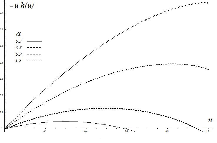
Figure 1: The function $-u\,h(u)=\alpha\,u+\frac{1}{3\leavevmode\nobreak\ u^{2}}\left[1-3\,\sqrt{1-u^{4}}+2\ {{}_{2}}F_{1}\left(-\frac{3}{4},\frac{1}{2};\frac{1}{4};u^{4}\right)\right]$ for different values of $\alpha$.

It is useful to compare our results with the solution to the usual Einstein-Born-Infeld (EBI) dynamics [18], which we summarize below. The functions $e(u)$ and $h(u)$ are

$$e_{EBI}=\frac{\beta^{-1}\leavevmode\nobreak\ u^{2}\leavevmode\nobreak\ \lambda}{\sqrt{1+\lambda^{2}u^{4}}}\leavevmode\nobreak\ ,\quad\quad h_{EBI}=-\int\leavevmode\nobreak\ du\leavevmode\nobreak\ u^{-4}\left(\lambda-\sqrt{1+\lambda^{2}u^{4}}\right)\ .$$ (80)

The geometry is singular at $u=\infty$ ($r=0$), and there can be two, one or no horizons depending on the relations between the parameters (see details in Ref. [19]). However the field invariant $S$ remains bounded,

$$S_{EBI}=-\frac{\beta^{-2}\leavevmode\nobreak\ u^{4}\leavevmode\nobreak\ \lambda^{2}}{2(1+\lambda^{2}u^{4})}\leavevmode\nobreak\ .$$ (81)

In the weak field region the metric takes the form

$$g_{00\ EBI}=1-\frac{\beta^{2}M}{\epsilon\,r}-\frac{\Lambda}{3}\leavevmode\nobreak\ r^{2}+\frac{(\beta Q\lambda)^{2}}{2\epsilon\,r^{2}}-\frac{(\beta Q\lambda)^{4}}{40\epsilon\,r^{6}}+O(r^{-9})\leavevmode\nobreak\ ,$$ (82)

which exhibits subtle differences with respect to Eq. (77) coming from different signs and the different role of $\lambda$ in $h_{EBI}(u)$ as compared to $h(u)$ (see Eqs. (73) and (80)).

VI Summary and Conclusion

We have studied the field equations coming from a Born-Infeld-type determinantal Lagrangian that linearly combines gravity and matter, when varied within a metric-affine (à la Palatini) framework. This formulation explicitly violates the postulates of metric theories of gravity (MTG) by construction, which raised concerns about its compatibility with the Einstein equivalence principle. However, by carefully analyzing the field equations when the matter sector is described by an electromagnetic field, we have shown that the dynamics of the theory can be equivalently obtained from an MTG action which adds the (Einstein-Hilbert) GR action to a Born-Infeld electrodynamics theory with a “wrong” sign. This result is exact and independent of the symmetries of the particular solution presented in Section V. The appearance of a non-standard sign in the electromagnetic sector prevents the bound of the corresponding invariants, which leads to undesired physical properties.

It is important to note that the methods introduced here to deal with the inverse of the tensor $q_{\mu\nu}$ are generic and can be applied whenever an antisymmetric part appears in the linear combination that defines $q_{\mu\nu}$. Thus, more general electromagnetic scenarios and combinations of different matter fields can be tackled following a similar procedure. Despite the fact that the model considered here does not prevent curvature divergences, the possibility of more general actions that result in regularized geometric and matter sectors cannot be ruled out. Thanks to our results, such theories are now accessible to exploration and new results will be reported elsewhere soon.

Appendix A Born-Infeld equation derivation

To obtain the antisymmetric part of $\hat{q}^{-1}$ we first write the relation (in matrix form)

$$\hat{q}^{-1}=(\hat{\cal G}+\beta\hat{F})^{-1}=(\hat{I}+\beta\,\hat{\cal G}^{-1}\hat{F})^{-1}\hat{\cal G}^{-1}=\left(\sum_{n=0}^{\infty}(-\beta)^{n}(\hat{\cal G}^{-1}\hat{F})^{n}\right)\hat{\cal G}^{-1}$$ (83)

Noting that $\hat{\cal G}^{-1}\hat{F}={\cal G}^{\mu\alpha}F_{\alpha\mu}=\tilde{F}^{\mu}_{\ \nu}$, and using the properties (13) and (14) of antisymmetric tensors, it is straightforward to show that the series expansion above can only have four kinds of terms, namely,

$$\sum_{n=0}^{\infty}(-\beta)^{n}(\hat{\cal G}^{-1}\hat{F})^{n}=\tilde{H}\left(\delta^{\mu}_{\ \beta}-\beta\tilde{F}^{\mu}_{\ \beta}+\beta^{2}{\,{}^{\star}\!}\tilde{F}^{\mu}_{\ \alpha}{\,{}^{\star}\!}\tilde{F}^{\alpha}_{\ \beta}+\beta^{3}\tilde{P}{\,{}^{\star}\!}\tilde{F}^{\mu}_{\ \beta}\right)\ ,$$ (84)

where the overall scalar factor $\tilde{H}$ can be directly identified by solving the identity

$$\hat{I}=(\hat{I}+\beta\hat{\cal G}^{-1}\hat{F})^{-1}(\hat{I}+\beta\hat{\cal G}^{-1}\hat{F})=\tilde{H}\left(\delta^{\mu}_{\beta}-\beta\tilde{F}^{\mu}_{\ \beta}+\beta^{2}{\,{}^{\star}\!}\tilde{F}^{\mu}_{\ \alpha}{\,{}^{\star}\!}\tilde{F}^{\alpha}_{\ \beta}+\beta^{3}\tilde{P}{\,{}^{\star}\!}\tilde{F}^{\mu}_{\ \beta}\right)(\delta^{\beta}_{\nu}+\beta\tilde{F}^{\beta}_{\ \nu}) = \delta^{\mu}_{\nu}\ ,$$ (85)

from which we get $\tilde{H}=\left(1+\beta^{2}2\tilde{S}-\beta^{4}\tilde{P}^{2}\right)^{-1}.$ Thus, the inverse of $q_{\mu\nu}$ in terms of the inverse of ${\cal G}_{\mu\nu}$ reads

$$q^{\mu\nu} = \frac{\tilde{\cal G}^{\mu\nu}-\beta{\tilde{F}}^{\mu\nu}+\beta^{2}{\,{}^{\star}\!}{\tilde{F}}^{\mu}_{\ \ \alpha}{\,{}^{\star}\!}\tilde{F}^{\alpha\nu}+\beta^{3}\tilde{P}{\,{}^{\star}\!}\tilde{F}^{\mu\nu}}{1+\beta^{2}2\tilde{S}-\beta^{4}\tilde{P}^{2}}\ .$$ (86)

Extracting the antisymmetric part of (86) and using that ${\,{}^{\star}\!}{\tilde{F}}^{[\mu}_{\ \ \alpha}{\,{}^{\star}\!}\tilde{F}^{\nu]\alpha}=0$, and that ${\cal G}_{\mu\nu}$ is symmetric and non-singular by definition and therefore $\tilde{\cal G}^{[\mu\nu]}=0$, we get

$$\left(\hat{q}^{-1}\right)^{[\mu\nu]} = -\beta\frac{{\tilde{F}}^{\mu\nu}-\beta^{2}\tilde{P}{\,{}^{\star}\!}\tilde{F}^{\mu\nu}}{1+\beta^{2}2\tilde{S}-\beta^{4}\tilde{P}^{2}}\ .$$ (87)

On the other hand, writing $q_{\mu\nu}$ as $q_{\mu\nu}={\cal G}_{\mu\rho}(\delta^{\rho}_{\ \nu}+\beta\tilde{F}^{\rho}_{\ \nu})\,,$ its squared root determinant takes the form

$$\sqrt{-q} = \sqrt{-{\cal G}}\sqrt{\det(\delta^{\rho}_{\ \nu}+\beta\tilde{F}^{\rho}_{\ \nu})}=\sqrt{-{\cal G}}\sqrt{1+2\beta^{2}\tilde{S}-\beta^{4}\tilde{P}^{2}}\ ,$$ (88)

So, using (22), we can finally write down

$$\sqrt{-q}\left[\hat{q}^{-1}\right]^{[\mu\nu]}=-\beta\sqrt{-{\cal G}}\frac{{\tilde{F}}^{\mu\nu}-b^{-2}\tilde{P}{\,{}^{\star}\!}\tilde{F}^{\mu\nu}}{\sqrt{1+2b^{-2}\tilde{S}-b^{-4}\tilde{P}^{2}}}=-\beta\sqrt{-{\cal G}}\widetilde{\cal F}^{\mu\nu}\ ,$$ (89)

which proves the equation (20).

References

• [1] M. Born and L. Infeld, Proc. Roy. Soc. Lond. A 144, no.852, 425-451 (1934) doi:10.1098/rspa.1934.0059
• [2] E. S. Fradkin and A. A. Tseytlin, Phys. Lett. B 163, 123-130 (1985) doi:10.1016/0370-2693(85)90205-9
• [3] S. Deser and G. W. Gibbons, Class. Quant. Grav. 15, L35-L39 (1998) doi:10.1088/0264-9381/15/5/001 [arXiv:hep-th/9803049 [hep-th]].
• [4] D. N. Vollick, Phys. Rev. D 69, 064030 (2004) doi:10.1103/PhysRevD.69.064030 [arXiv:gr-qc/0309101 [gr-qc]].
• [5] M. Banados and P. G. Ferreira, Phys. Rev. Lett. 105, 011101 (2010) [erratum: Phys. Rev. Lett. 113, no.11, 119901 (2014)] doi:10.1103/PhysRevLett.105.011101 [arXiv:1006.1769 [astro-ph.CO]].
• [6] J. Beltran Jimenez, L. Heisenberg, G. J. Olmo and D. Rubiera-Garcia, Phys. Rept. 727, 1-129 (2018) doi:10.1016/j.physrep.2017.11.001 [arXiv:1704.03351 [gr-qc]].
• [7] C.M. Will, Theory and experiment in gravitational physics, Cambridge University Press, New York (1993).
• [8] C. M. Will, Living Rev. Rel. 17, 4 (2014) doi:10.12942/lrr-2014-4 [arXiv:1403.7377 [gr-qc]].
• [9] A. Delhom, Eur. Phys. J. C 80, no.8, 728 (2020) doi:10.1140/epjc/s10052-020-8330-y [arXiv:2002.02404 [gr-qc]].
• [10] D. N. Vollick, Phys. Rev. D 72, 084026 (2005) doi:10.1103/PhysRevD.72.084026 [arXiv:gr-qc/0506091 [gr-qc]].
• [11] G. J. Olmo, Int. J. Mod. Phys. D 20 (2011) 413.
• [12] V. I. Afonso, C. Bejarano, J. Beltran Jiménez, G. J. Olmo, and E. Orazi, Class. Quant. Grav.  34, no. 23, 235003 (2017)
• [13] J. Beltrán Jiménez and A. Delhom, Eur. Phys. J. C 79 (2019) no.8, 656
• [14] D. Sáez-Chillón Gómez, Phys. Lett. B 814 (2021), 136103
• [15] J. Beltran Jiménez and A. Delhom, Eur. Phys. J. C 80, 585 (2020)
• [16] R. Ferraro, J. High Energ. Phys. 2010, 28 (2010).
• [17] C. Bejarano, A. Delhom, A. Jiménez-Cano, G. J. Olmo and D. Rubiera-Garcia, Phys. Lett. B 802 (2020), 135275
• [18] A. García, H. Salazar, and J.F. Plebański, Nuov Cim B 84, 65-90 (1984).
• [19] N. Bretón, Class. Quantum Grav. 19, 601-612 (2002).