Algorithm Design:
A Fairness-Accuracy Frontier

Abstract.

Algorithm designers increasingly optimize not only for accuracy, but also for the fairness of the algorithm across pre-defined groups. We study the tradeoff between fairness and accuracy for any given set of inputs to the algorithm. We propose and characterize a fairness-accuracy frontier, which consists of the optimal points across a broad range of preferences over fairness and accuracy. Our results identify a simple property of the inputs, group-balance, which qualitatively determines the shape of the frontier. We further study an information-design problem where the designer flexibly regulates the inputs (e.g., by coarsening an input or banning its use) but the algorithm is chosen by another agent. Whether it is optimal to ban an input generally depends on the designer’s preferences. But when inputs are group-balanced, then excluding group identity is strictly suboptimal for all designers, and when the designer has access to group identity, then it is strictly suboptimal to exclude any informative input.

1. Introduction

Suppose a hospital uses a machine learning algorithm to aid in the diagnosis of a medical condition, where the algorithm makes the correct diagnosis 90% of the time for Blue patients and 50% of the time for Red patients. Such an outcome—where the consequences of a policy differ systematically across two groups—is known as disparate impact. A recent literature demonstrates that algorithms used across a wide range of applications have disparate impact (Arnold, Dobbie, and Hull, 2021; Fuster, Goldsmith-Pinkham, Ramadorai, and Walther, 2021). For example, patients assigned the same risk score by a healthcare algorithm were shown to have substantially different actual health risks depending on their race (Obermeyer, Powers, Vogeli, and Mullainathan, 2019); the false-positive rate of an algorithm used to predict criminal reoffense was shown to be twice as high for Black defendants as for White defendants (Angwin and Larson, 2016); and the accuracy of facial-recognition technologies vary substantially across demographic groups (Klare et al., 2012).

Policymakers prefer for algorithms to have lower disparate impact but would also like for these algorithms to be more accurate. Ideally these goals would be achieved together; in practice, there may be intrinsic tradeoffs between accuracy (the overall error rate of the algorithm) and fairness (how similar the error rates are across pre-defined groups). This tradeoff is governed in part by the inputs to the algorithm, which can be observed, manipulated, and regulated—raising the following fundamental questions: How does the tradeoff between fairness and accuracy depend on the information available for prediction? Which informational environments create a tension between fairness and accuracy, and which ameliorate it? While the tradeoff between fairness and accuracy has been empirically computed in specific applications (Wei and Niethammer, 2020; Chohlas-Wood et al., 2021; Little et al., 2022), we know substantially less about how the available information shapes the tension between these objectives in general.

To examine these questions, we define and study a fairness-accuracy frontier. The frontier consists of those outcomes that are optimal for a broad class of objective functions, which reflect different views on how to trade off fairness and accuracy. We prove two types of results about the frontier. First, we identify simple properties of the algorithmic inputs that determine the qualitative shape of this frontier. Second, we take an information-design perspective on understanding how constraints on information can induce certain desired outcomes. Specifically, we consider an interaction between a regulator flexibly constraining the inputs and an agent setting the algorithm, and characterize what part of the fairness-accuracy frontier the designer can achieve through appropriate design of the inputs. We also examine whether it might be optimal for the designer to exclude an input altogether (e.g., excluding group identity in the context of medical predictions).

In our model, a designer chooses an algorithm that takes observed covariates as inputs (e.g., image scans, lab tests, records of prior hospital visits) and outputs a decision (e.g., whether to recommend a medical procedure). The algorithm’s consequences for any given individual are measured using a loss function, which can be interpreted as the inaccuracy or the harm of the decision. We aggregate losses within two groups, group $r$ (Red) and group $b$ (Blue). Each group’s error is the expected loss for individuals of that group. An algorithm is understood to be more accurate if it implies lower errors for both groups, and more fair if it implies a smaller absolute difference between the two groups’ errors.

To understand the tradeoff between fairness and accuracy, we define the class of fairness-accuracy (FA) preferences to be all preferences over group errors that are consistent with the following order: one pair of group errors FA-dominates another if the former involves smaller errors for both groups (greater accuracy) and also a smaller difference between group errors (greater fairness). This partial order is consistent with a broad range of designer preferences, including Utilitarian designers (who minimize the aggregate error in the population), Rawlsian designers (who minimize the greater of the two group errors), and Egalitarian designers (who minimize the absolute difference between group errors). Some of these preferences also correspond directly to optimization problems that have been proposed for use in practice. We define the fairness-accuracy frontier to be the set of all feasible group error pairs that are FA-undominated within the feasible set, i.e., there is no feasible error pair that improves simultaneously on both accuracy and fairness.

A simple property of the algorithm’s inputs turns out to be critical for determining the shape of the fairness-accuracy frontier. Say that a covariate vector is group-balanced if a group’s optimal algorithm (i.e. the one that gives that group the smallest error over all feasible algorithms) yields a lower error for that group than for the other group. Otherwise, say that the covariate vector is group-skewed. While it may be difficult to anticipate in advance of an empirical analysis whether group-balance or group-skew is more typical in practice, one scenario in which the latter may arise is if covariates have the same implications for both groups but are measured more accurately for one group than the other (e.g. medical data is recorded more accurately for high-income patients than low-income patients).

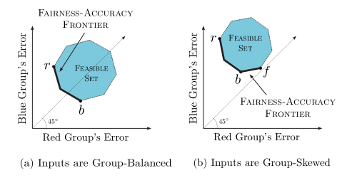
Figure 1. The Fairness-Accuracy Frontier.

Our first result says that depending on whether the covariate vector is group-balanced or group-skewed, the fairness-accuracy frontier takes either of two possible forms, as depicted in Figure 1. In both cases, the frontier is a part of the lower boundary of the feasible set, namely the error pairs that are implementable using some algorithm that takes the covariate vector as input. In the case of group-balanced inputs, the fairness-accuracy frontier is the part of the lower boundary that begins at the point that is best for group Red (labeled $r$) and ends at the point that is best for group Blue (labeled $b$). This is precisely the standard Pareto frontier, i.e. the set of all feasible error pairs that cannot be simultaneously reduced in both coordinates. In the case of group-skewed inputs, the fairness-accuracy frontier is larger than the standard Pareto frontier, additionally including a positively-sloped part (in Figure 1, the segment from $b$ to the fairness-maximizing point $f$) along which both groups’ errors increase but the gap between their errors decreases. We can conclude from this characterization that a policy proposal that increases errors for both groups, but reduces the gap between group errors, can never be justified by fairness considerations if the covariate vector is group-balanced, but can be justified in some cases if it is group-skewed.

We next consider the important special case where group identity is an input to the algorithm. We show that the feasible set and frontier simplify as depicted in Figure 2: the feasible set is a rectangle, and the fairness-accuracy frontier is a single line segment along which the disadvantaged group (i.e., the group with the higher error) receives its minimal feasible error. If we consider a comparative static exercise in which a baseline covariate vector is augmented to include group identity, then a corollary of this characterization is that access to group identity must reduce the error for the worse-off group, regardless of the designer’s fairness-accuracy preferences.

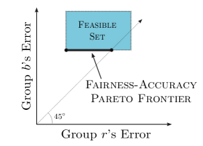
Figure 2. Depiction of the fairness-accuracy frontier in the case where $X$ reveals $G$.

In the second part of the paper, we investigate what happens if the designer does not choose the algorithm, but instead regulates the inputs of the algorithm. This question is motivated by settings where a designer has fairness concerns, but another agent setting the algorithm does not. For example, a healthcare provider (agent) determining treatment may seek to maximize the number of correct diagnoses, while a policymaker (designer) may additionally prefer that the accuracy of the provider’s treatments be equitable across certain social groups. In these cases, the policymaker can impose regulation that restricts the inputs available to the algorithm, for example by banning the use of a specific input.

We model this as an information design problem (Kamenica and Gentzkow, 2011) where the designer chooses a garbling of the available inputs, and an agent chooses an algorithm (based on the garbling) to maximize accuracy. Under weak conditions, it turns out to be without loss for the designer to only control the algorithm’s inputs. That is, any error pair that a designer would choose to implement given full control of the algorithm can also be achieved by appropriately garbling the inputs.

Might the optimal garbling involve completely excluding a covariate from use in the algorithm? We demonstrate two results: First, excluding group identity as an algorithmic input is strictly welfare-reducing for all designers (with FA preferences) if and only if the permitted covariates are group-balanced. Second, when group identity is permitted as an input, then completely excluding any other covariate makes every designer strictly worse off, so long as that covariate satisfies a mild condition that we call decision-relevance. We could apply these results to the policy question of whether to permit standardized test scores in admissions decisions. In this case, the latter result suggests that so long as group identity is a permissible input in admission decisions, then excluding test scores is welfare-reducing for all designers with the power to garble covariates. On the other hand, if group identity is not permitted as an input in college admissions decisions (as is the case in California and Michigan), then the optimal garbling of covariates for some designer preference may indeed involve completely excluding test scores, and we provide a simple example to illustrate this effect.

1.1. Related Literature

Our paper is motivated by recent problems regarding algorithmic bias (Section 1.1.3), but adopts a novel perspective on these questions based on approaches from two literatures in economic theory: the literature on information design (Section 1.1.1) and the literature on social preferences and inequality (Section 1.1.2). Building on the former, we model the interaction between a designer flexibly regulating inputs and an agent setting the algorithm. Building on the latter, we focus on understanding equity-efficiency tradeoffs, and consider a wide class of preferences that reflects heterogeneity in social preferences.

1.1.1. Information Design

One contribution of our paper is the casting of the design of algorithmic inputs as an information design problem (see Kamenica (2019) and Bergemann and Morris (2019) for recent surveys). This approach complements previous frameworks for modeling the regulation of algorithms, in which regulators communicate information via cheap talk (Cowgill and Stevenson, 2020) or impose restrictions directly on the algorithm (Yang and Dobbie, 2020; Rambachan, Kleinberg, Mullainathan, and Ludwig, 2021; Blattner, Nelson, and Spiess, 2022). We view the garbling of inputs as a potentially effective policy tool, which can be implemented through a variety of technological or legal commitments, and which deserves further attention within the context of algorithmic fairness.

Conversely, problems regarding algorithmic fairness motivate analyses that depart from typical information design problems in a few interesting ways. First, the Sender in our framework cannot choose a completely flexible information structure, but is instead constrained to garblings of a primitive covariate vector.

Second, motivated by heterogeneous attitudes toward fairness (Section 1.1.2), we focus on a frontier of solutions with respect to a wide class of Sender preferences. Our results in Section 4.2 describe how the frontier of solutions responds to changes in the underlying information. We focus on special cases of this comparative static that are of interest given our motivation (e.g., adding or removing a covariate), but a more general solution (analogous to Curello and Sinander (2022)’s work on comparative statics with respect to the Sender’s utility function) would be an interesting avenue for future work.

Finally, at the broader intersection of information design and algorithms, Ichihashi (2023) considers optimal information acquisition for crime deterrence, and Caplin, Martin, and Marx (2023) draws a connection between different machine learning objectives and costly information design.

1.1.2. Social Preferences and Inequality

The literature on social preferences documents substantial heterogeneity in how individuals assess efficiency-equity tradeoffs (Andreoni and Miller, 2002; Fehr and Schmidt, 1999; Fisman, Kariv, and Markovits, 2007; Sullivan, 2022), which is reflected in our broad class of FA-preferences. In this literature, social preferences are preferences over individual payoffs rather than preferences over group errors, but most have analogues in our setting. For example, the “social welfare approach” aggregates individual payoffs using differential weights (Charness and Rabin, 2002; Saez and Stantcheva, 2016; Dworczak, Kominers, and Akbarpour, 2021), and is nested in our class of FA preferences (if we interpret individual payoffs as group errors). We additionally allow for a direct penalty for unequal outcomes, as in the models of “difference aversion” or “inequity aversion” (Loewenstein et al., 1989; Fehr and Schmidt, 1999; Bolton and Ockenfels, 2000).

There is a separate literature studying the equity-efficiency tradeoffs of affirmative action programs. Specifically, Lundberg (1991) and Chan and Eyster (2003) model affirmative action as a ban on the use of group identity in admissions decisions, and show that this can lead organizations to condition on proxies in a way that reduces both efficiency and equity. (A similar point is made in Agan and Starr (2018) regarding the use of prior criminal history in hiring decisions in “ban-the-box” policies.) Ellison and Pathak (2021) empirically quantify the equity and efficiency losses of race-neutral affirmative action (based on geographic proxies for race) as compared to plans that explicitly consider race. These papers are related to our study of the impact of excluding group identity, but focus on how a designer’s optimal algorithm given group identity compares to the optimal algorithm without. We instead examine how the frontier of achievable outcomes changes when the designer can design a group-dependent garbling versus when the designer must choose a group-independent garbling. These analyses are not nested; see Section 4.2.1 for more detail.

1.1.3. Algorithmic Bias

The recent literature on algorithmic bias has emerged around the concern that algorithms have error rates that differ substantially across social and demographic groups (see Kleinberg et al. (2018) and Cowgill and Tucker (2020) for overviews). In this literature and in the accompanying policy discussion (e.g, Angwin and Larson (2016)), algorithms are often considered to be “less fair” if the harms of the algorithm are more unequally borne across groups, with this comparison formalized as a larger disparity in error rates across groups (Hardt et al., 2016; Kleinberg et al., 2017; Chouldechova, 2017). A growing body of empirical work documents and quantifies these disparate impacts (Obermeyer et al., 2019; Arnold et al., 2021; Fuster et al., 2021).

The tradeoff between accuracy (overall error rate of the algorithm in the population) and fairness (discrepancy between error rates across social groups) is a special kind of equity-efficiency tradeoff. A common approach for resolving this tradeoff is to posit a particular objective criterion (Hardt et al., 2016; Diana et al., 2021). Other papers identify improvements with respect to both objectives simultaneously (Rose, 2021; Feigenberg and Miller, 2021). Our paper is closest to a smaller part of this literature, which engages with the tension between fairness and accuracy by quantifying fairness-accuracy tradeoffs for specific loss functions (Menon and Williamson, 2018) or for specific empirical applications (Wei and Niethammer, 2020; Chohlas-Wood et al., 2021; Little et al., 2022). We are interested in how this fairness-accuracy tradeoff is moderated by the inputs to the algorithm in general, and provide simple conditions on the inputs that qualitatively govern this tradeoff independently of other details of the loss function or informational environment.

2. Framework

2.1. Setup and Notation

There is a population of individuals, where each individual is described by a covariate vector $X$ taking values in the finite set $\mathcal{X}$, a type $Y$ taking values in the finite set $\mathcal{Y}$, and a group identity $G$ taking values $r$ or $b$. Throughout we think of $G,X,Y$ as random variables with joint distribution $\mathbb{P}$, and use $p_{g}\equiv\mathbb{P}(G=g)>0$ to denote the fraction of the population that belongs to group $g\in\{r,b\}$. We impose no assumptions on the joint distribution, permitting for example each of the following:

Example 1 ($X$ reveals or closely proxies for $G$).

The group identity may be an input in the covariate vector $X$, or predictable from inputs in the covariate vector $X$. For example, Bertrand and Kamenica (2020) show that data on consumption patterns permits near perfect classification of gender and a fairly accurate prediction of other group identities such as income bracket, race, and political ideology.

Example 2 (Biased Covariates).

The value of an input in $X$ may be systematically biased depending on group identity. For example, if $G$ is income bracket, $Y$ is ability, and $X$ is a test score that can be improved through better access to test prep, the distribution $\mathbb{P}$ may have the property that at every ability level, the conditional distribution of test scores is shifted higher for students in the high-income bracket (i.e., the distribution of $X\mid Y=y,G=r$ first-order stochastically dominates $X\mid Y=y,G=b$ at every $y\in\mathcal{Y}$).

Example 3 (Asymmetrically Informative Covariates).

The inputs in $X$ may be more informative about $Y$ for one group than the other. For example, in Obermeyer et al. (2019), a patient’s health care costs are more predictive of their health care needs for White patients than for Black patients, and Rothstein (2004) shows that SAT scores are more informative about future college grades for high-income students than low-income students.

A designer chooses an algorithm $a:\mathcal{X}\rightarrow\Delta(\mathcal{D})$ that maps covariate vectors into distributions over decisions in $\mathcal{D}=\{0,1\}$. We use $\mathcal{A}_{X}$ to denote the set of all algorithms. Some motivating examples of types, group identities, covariate vectors, and decisions are given below:

Healthcare. $Y$ is need of treatment, $G$ is socioeconomic class, and the decision is whether the individual receives treatment. The covariate vector $X$ includes possible attributes such as image scans, number of past hospital visits, family history of illness, and blood tests.

Credit scoring. $Y$ is creditworthiness, $G$ is gender, and the decision is whether the borrower’s loan request is approved. The covariate vector $X$ includes possible attributes such as purchase histories, social network data, income level, and past defaults.

Bail. $Y$ is whether an individual is high-risk or low-risk of criminal reoffense, $G$ is race, and the decision is whether the individual is released on bail. The covariate vector $X$ includes possible attributes such as the individual’s past criminal record, psychological evaluations, family criminal background, frequency of moves, or drug use as a child.

Job hiring. $Y$ is whether a job applicant is high or low quality, $G$ is citizenship, and the decision is whether the applicant is hired. The covariate vector $X$ includes possible attributes such as past work history, resume, and references.

The consequence of choosing decision $d$ for an individual whose true type is $y$ is evaluated using a loss function $\ell:\mathcal{D}\times\mathcal{Y}\rightarrow\mathbb{R}$, which we view as a measure of inaccuracy independent of fairness. We further aggregate these losses across individuals within each group:

Definition 2.1.

For any algorithm $a\in\mathcal{A}_{X}$ and group $g\in\{r,b\}$, the group $g$ error is

$$e_{g}(a):=\mathbb{E}_{D\sim a(X)}\left[\ell(D,Y)\mid G=g\right].$$

That is, group $g$’s error is the average loss for members of group $g$. For example, if the type $Y$ is binary and $\ell(d,y)=\mathbbm{1}(d\neq y)$, then $e_{g}(a)$ is the total probability of a type I or type II error. Other loss functions may put different weights on different kinds of errors. We view the choice of the right loss function as application-specific, and demonstrate results that hold for arbitrary $\ell$.

Each algorithm $a$ implies a pair of group errors $(e_{r}(a),e_{b}(a))$. Throughout this paper, we use an improvement in accuracy to mean a reduction in both group errors, and an improvement in fairness to mean a reduction in the absolute difference between the group errors. This approach nests many of the various fairness criteria that have been proposed in the literature (see Mehrabi et al. (2022) for a recent survey) as a particular choice of a loss function. For example, if the type $Y$ is binary and $\ell(d,y)=\mathbbm{1}(d\neq y)$, then $e_{r}(g)=e_{b}(g)$ corresponds to equality of misclassification rates, while if $\ell(d,y)=\mathbbm{1}(d=1,y=0)$ then $e_{r}(g)=e_{b}(g)$ corresponds to equality of false positive rates (Kleinberg et al., 2017; Chouldechova, 2017). See Appendix O.7 for further details and examples.

In Section 5, we discuss an extension of the fairness criterion to any $|\phi(e_{r})-\phi(e_{b})|$ where $\phi$ is continuous and strictly increasing, which includes the ratio of error rates as a special case (setting $\phi(e)=\log(e)$). We also discuss in Section 5 an extension of our framework when fairness and accuracy are evaluated using different loss functions.

2.2. Fairness-Accuracy Preferences

The designer has a preference ordering over group error pairs $e=(e_{r},e_{g})\in\mathbb{R}^{2}$. We consider the set of all preferences that are consistent with the following weak criterion.

Definition 2.2.

The fairness-accuracy (FA) dominance relation $>_{FA}$ is the partial order on $\mathbb{R}^{2}$ satisfying $e>_{FA}e^{\prime}$ if $e_{r}\leq e_{r}^{\prime}$, $e_{b}\leq e_{b}^{\prime}$, and $|e_{r}-e_{b}|\leq|e_{r}^{\prime}-e_{b}^{\prime}|$, with at least one inequality strict.

That is, if it is possible to simultaneously increase accuracy (reducing errors for both groups) and also increase fairness (reducing the gap between these errors), then all designers must prefer this.

Definition 2.3.

A fairness-accuracy (FA) preference $\succeq$ is any total order on $\mathbb{R}^{2}$ such that $e\succ e^{\prime}$ whenever $e>_{FA}e^{\prime}$.

It is straightforward to see that these orders are unchanged if $|e_{r}-e_{b}|$ is replaced with $\phi(|e_{r}-e_{b}|)$ where $\phi$ is a strictly increasing function.

The class of FA preferences reflects a broad range of views on how to trade off fairness and accuracy, including the following special cases that have been proposed in the literature.

Example 4 (Utilitarian).

The designer evaluates errors $e=\left(e_{r},e_{b}\right)$ according to the weighted sum in the population. That is, let $w_{u}(e)=-p_{r}e_{r}-p_{b}e_{b}$, and let $\succeq_{u}$ be the ordering represented by $w_{u}$, so that $e\succeq_{u}e^{\prime}$ if and only if $w_{u}(e)\geq w_{u}(e^{\prime})$. (Note that the minority population, which has a lower weight by definition, will be naturally discounted as a group in this evaluation.) A designer with preferences $\succeq_{u}$ is called Utilitarian (Harsanyi, 1953, 1955).

Example 5 (Social Welfare Approach).

A generalization of the Utilitarian rule instead evaluates errors $e$ using $w_{\alpha}(e)=-\alpha_{r}e_{r}-\alpha_{b}e_{b}$ for arbitrary positive constants $\alpha_{r},\alpha_{b}$ (Charness and Rabin, 2002; Saez and Stantcheva, 2016; Dworczak, Kominers, and Akbarpour, 2021; Rambachan, Kleinberg, Mullainathan, and Ludwig, 2021).

Example 6 (Rawlsian).

The designer evaluates errors $e=\left(e_{r},e_{b}\right)$ according to the greater error. That is, let $w_{r}(e)=-\max\left\{e_{r},e_{b}\right\}$, and let $\succeq_{r}$ be the corresponding ordering represented by $w_{r}$. A designer with preferences $\succeq_{r}$ is called Rawlsian (Rawls, 1971).

Example 7 (Egalitarian).

The designer evaluates errors $e=\left(e_{r},e_{b}\right)$ according to their difference. That is, let $w_{e}(e)=-\left|e_{r}-e_{b}\right|$, and let $\succeq_{e}$ be the lexicographic order that first evaluates errors according to $w_{e}$ and then compares ties using the Utilitarian utility $w_{u}$. A designer with preferences $\succeq_{e}$ is called Egalitarian.

Example 8 (Constrained Optimization).

The designer evaluates errors $e=\left(e_{r},e_{b}\right)$ according to $w_{c}\left(e\right)=\left(1-\lambda\right)w_{u}\left(e\right)+\lambda w_{e}\left(e\right)$ for some $\lambda\in[0,1]$ (breaking ties with $\succeq_{e}$ when $\lambda=1$). The optimal choices here correspond to the solutions of the following constrained optimization problem

$$\min_{a\in\mathcal{A}_{X}}p_{r}e_{r}(a)+p_{b}e_{b}(a)\text{ s.t. }\left|e_{r}(a)-e_{b}(a)\right|\leq c$$

when the constraint is satisfiable. The special case of $c=0$ (as considered in Hardt et al. (2016)) returns the Egalitarian solution.

Example 9 (Accuracy then Fairness).

The designer evaluates errors $e=\left(e_{r},e_{b}\right)$ by first evaluating accuracy and then fairness. That is, $e\succ e^{\prime}$ if $e_{r}\leq e_{r}^{\prime}$ and $e_{b}\leq e_{b}^{\prime}$ with at least one strict, and if not, they are then compared using $w_{e}$. This is the approach recently proposed by Viviano and Bradic (2023).

Our consideration of this wide class of preferences is motivated in part by the experimental literature on social preferences, which documents substantial heterogeneity across individuals’ equity-efficiency preferences. For example, when given the choice between different allocations of payoffs across individuals, some experimental subjects choose Pareto-dominated allocations that are more equal (corresponding in our setting to choice of $(e_{r},e_{b})$ over $(e_{r}^{\prime},e_{b}^{\prime})$ where $e_{r}>e_{r}^{\prime}$ and $e_{b}>e_{b}$ but $|e_{r}-e_{b}|<|e_{r}^{\prime}-e_{b}^{\prime}|$). These are minority preferences in the population (Andreoni and Miller, 2002; Charness and Rabin, 2002), but constitute 31% of subjects in an experiment in Fisman et al. (2007). We do not take a normative stance on which FA preferences are more appropriate, instead viewing the class of FA preferences as encompassing a broad range of designer preferences that may be relevant in practice.

2.3. The Fairness-Accuracy Frontier

Fixing any covariate vector $X$, we define the feasible set of group error pairs to be those pairs that can be implemented by some algorithm that takes $X$ as input. The fairness-accuracy frontier is the set of all group error pairs that are FA-undominated in the feasible set.

Definition 2.4.

The feasible set given covariate vector $X$ is

$$\mathcal{E}_{X}\equiv\{e(a):a\in\mathcal{A}_{X}\}.$$

Definition 2.5.

The fairness-accuracy (FA) frontier given $X$ is

$$\mathcal{F}_{X}\equiv\{e\in\mathcal{E}_{X}:\textrm{no }e^{\prime}\in\mathcal{E}_{X}\textrm{ such that }e^{\prime}>_{FA}e\}.$$

The FA frontier consists of all group error pairs that are optimal under some FA preference. It is minimal in the sense that every point in the FA frontier is uniquely optimal for some FA preference, so we cannot exclude any points without hurting some designer. See Appendix O.6 for further details and results, including an alternate characterization using a smaller class of “simple preferences.”

3. The Fairness-Accuracy Frontier

In Section 3.1, we define the property of group-balance that will play a key role in our results. In Section 3.2, we characterize the frontier and its implications for the kinds of fairness-accuracy tradeoffs that emerge. In Section 3.3, we provide further results for two important special cases: when group identity is an input in the algorithm and when group identity is independent of type conditional on the covariate vector.

3.1. Key Property: Group-Balance

For all covariate vectors $X$, the feasible set $\mathcal{E}_{X}$ is closed and convex (Lemma A.1). It includes the following special points.

Definition 3.1 (Group Optimal Points).

For any covariate vector $X$, define

$$r_{X}\equiv\operatorname*{arg\,min}_{e\in\mathcal{E}_{X}}e_{r}\textrm{\quad\quad\quad\quad}\displaystyle b_{X}\equiv\operatorname*{arg\,min}_{e\in\mathcal{E}_{X}}e_{b}$$

to be the feasible points that minimize group $r$’s error and group $b$’s error respectively. In both cases, if the minimizer is not unique, break ties by choosing the point that minimizes the other group’s error. We use $g_{X}$ to denote the group optimal point for group $g$.

Group optimal points can be easily derived. For instance, to calculate $r_{X}$, set the algorithm to choose the optimal decision for group $r$ for each realization of $X$ (breaking ties in favor of group $b$). $r_{X}$ is then the error pair resulting from this algorithm.

Definition 3.2 (Fairness Optimal Point).

For any covariate vector $X$, define

$$f_{X}\equiv\operatorname*{arg\,min}_{e\in\mathcal{E}_{X}}|e_{r}-e_{b}|$$

to be the point that minimizes the absolute difference between group errors. If the minimizer is not unique, we choose the point that further minimizes either group’s error.

While $r_{X}$ and $b_{X}$ respectively denote the points that minimize group $r$ and $b$’s errors, the group whose error is minimized need not be the group with the lower error. For example, suppose $X$ is a binary score where the conditional distribution $(X,Y)\mid G$ is described by:

$$\begin{array}[]{ccc}&X=0&X=1\\ Y=0&3/8&1/8\\ Y=1&1/8&3/8\end{array}\quad\quad\quad\begin{array}[]{ccc}&X=0&X=1\\ Y=0&1/3&1/6\\ Y=1&1/6&1/3\end{array}$$

$$G=r\hskip 142.26378ptG=b$$

Let the loss function $\ell$ be the misclassification rate; that is, $\ell(d,y)=\mathbbm{1}(d\neq y)$. Then the $b$-optimal point $b_{X}$ is achieved by the algorithm that maps $X=1$ to $d=1$ and $X=0$ to $d=0$, which leads to a higher error for group $b$ than group $r$ ($1/3$ compared to $1/4$). We will define such a covariate vector to be $r$-skewed.

Definition 3.3.

Covariate vector $X$ is:

• $r$-skewed if $e_{r}<e_{b}$ at $r_{X}$ and $e_{r}\leq e_{b}$ at $b_{X}$

• $b$-skewed if $e_{b}<e_{r}$ at $b_{X}$ and $e_{b}\leq e_{r}$ at $r_{X}$

• group-balanced otherwise

If $X$ is $g$-skewed for either group $g$, then we say it is group-skewed.

In words, $X$ is $r$-skewed if group $r$’s error is smaller than group $b$’s error not only at the $r$-optimal point $r_{X}$, but also at the $b$-optimal point $b_{X}$. Geometrically, this means that $r_{X}$ and $b_{X}$ fall to the same side of the 45 degree line. (The feasible set may however intersect with the 45 degree line, as in Figure 4.) In contrast, the covariate vector $X$ is group-balanced if at each group’s optimal point, its error is lower than that of the other group, implying that $r_{X}$ and $b_{X}$ fall to opposite sides of the 45 degree line.

Loosely speaking, a covariate vector is group-balanced if it is possible to disentangle accurate predictions for one group from accurate predictions for another. This might be, for example, because the meaning of the covariate vector is group-dependent (e.g., larger realizations of $X$ imply larger realizations of $Y$ for group $r$ but smaller realizations of $Y$ for group $b$), or because different covariates in the covariate vector are predictive for either group (e.g., $X=(X_{1},X_{2})$ where $X_{1}$ is uninformative about $Y$ for group $r$ and $X_{2}$ is uninformative about $Y$ for group $b$). In contrast, we would expect a covariate vector to be group-skewed if it is systematically more informative about one group than the other (e.g., if $Y\mid X=x,G=r$ is more dispersed than $Y\mid X=x,G=b$ for every $x$).

3.2. Characterization of the Frontier

Depending on whether the covariate vector $X$ is group-balanced or group-skewed, the fairness-accuracy frontier $\mathcal{F}_{X}$ takes either of two forms.

Theorem 3.1.

The fairness-accuracy frontier $\mathcal{F}_{X}$ is the lower boundary of the feasible set $\mathcal{E}_{X}$ between

• $r_{X}$ and $b_{X}$ if $X$ is group-balanced

• $g_{X}$ and $f_{X}$ if $X$ is $g$-skewed

These two cases are depicted in Figure 3. When $X$ is group-balanced and $r_{X}$ and $b_{X}$ are distinct, the two points fall on opposite sides of the 45-degree line (Panel (a)), and the fairness-accuracy frontier is that part of the lower boundary of the feasible set connecting these two points. This corresponds precisely to the set of all points $(e_{r},e_{b})$ such that no other feasible point $(e_{r}^{\prime},e_{b}^{\prime})$ is component-wise smaller, which we subsequently call the Pareto frontier. When $X$ is $r$-skewed (Panel (b)), then both $r_{X}$ and $b_{X}$ fall on the same side of the 45-degree line, and the fairness-accuracy frontier consists not only of the usual Pareto frontier connecting $r_{X}$ to $b_{X}$, but additionally a positively sloped line segment connecting the Pareto frontier to $f_{X}$.

Thus, the usual Pareto frontier and the fairness-accuracy frontier differ if and only if the covariate vector is group-skewed, implying the following corollary.

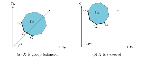
Figure 3. Example feasible set and fairness-accuracy frontier for (a) a group-balanced covariate vector $X$ and (b) an $r$-skewed covariate vector $X$.

Corollary 3.1.

Suppose $f_{X}$ is distinct from $r_{X}$ and $b_{X}$. Then if and only if $X$ is group-skewed, there are points $e,e^{\prime}\in\mathcal{F}_{X}$ satisfying $e_{r}\leq e^{\prime}_{r}$ and $e_{b}\leq e_{b}^{\prime}$ with at least one inequality strict.

This corollary says that if the covariate vector is group-balanced, then no two points on the fairness-accuracy frontier can be Pareto-ranked. Thus, a policy proposal that increases errors for both groups, but reduces the gap between group errors, cannot be optimal under any fairness-accuracy preference. On the other hand, if inputs are group-skewed, then the frontier has a positively-sloped segment along which every pair of points can be Pareto-ranked. On this part of the frontier, the only way to decrease the gap in errors (given the available information) is to increase errors for both groups. In practice, moving along this part of the frontier could correspond to choosing to ignore certain available information.

Suppose it were possible to acquire new covariates that turned a group-skewed covariate vector into a group-balanced covariate vector. Corollary 3.1 implies that such a change would not only (weakly) improve the fairness-accuracy frontier, but also change the nature of the fairness-accuracy conflict, eliminating the need to consider Pareto-dominated outcomes as a means to improve fairness. We leave to future work a more detailed exploration of endogenously chosen covariates and their fairness-accuracy consequences.

3.3. Special Cases

In the important case where group identity is an algorithmic input, the feasible set and fairness-accuracy frontier simplify further.

Definition 3.4.

Say that $X$ reveals $G$ if the conditional distribution $G\mid X=x$ is degenerate for every realization $x$ of $X$.

Proposition 3.1.

Suppose $X$ reveals $G$. Then the feasible set $\mathcal{E}_{X}$ is a rectangle whose sides are parallel to the axes, and the fairness-accuracy frontier $\mathcal{F}_{X}$ is the line segment from $r_{X}=b_{X}$ to $f_{X}$.

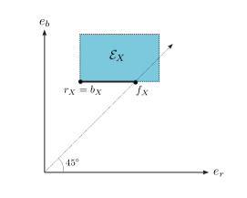
Figure 4. Example feasible set and fairness-accuracy frontier when $X$ reveals $G$.

An example of such a feasible set and fairness-accuracy frontier are depicted in Figure 4. One endpoint, the Utilitarian-optimal point labeled $r_{X}=b_{X}$, gives both groups their minimal feasible error. The other endpoint, the Egalitarian-optimal $f_{X}$, maximizes fairness. Everywhere along the fairness-accuracy frontier $\mathcal{F}_{X}$, the worse-off (higher error) group receives its minimal feasible error, so every point on the frontier is optimal for a Rawlsian designer. It is straightforward to see from this result that if we consider augmenting any covariate vector $X$ to include $G$, the error for the group that was “worse-off” under $X$ (i.e., had the higher error) must reduce regardless of which FA preference the designer holds.

Another interesting class of covariate vectors (nesting the previous one) are those that satisfy the following conditional independence property.

Definition 3.5.

Say that $X$ induces conditional independence if $G\perp\!\!\!\perp Y\mid X$.

A covariate vector that satisfies this property contains all of the information in group identity that is relevant for predicting $Y$, so that once $X$ is observed then there is no additional predictive value to knowing a subject’s group identity.

Proposition 3.2.

Suppose $X$ induces conditional independence. Then $\mathcal{F}_{X}$ is that part of the lower boundary of the feasible set $\mathcal{E}_{X}$ from the point $b_{X}=r_{X}$ to the point $f_{X}$.

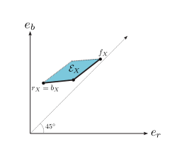
Figure 5. Depiction of the fairness-accuracy frontier under conditional independence of $G$ and $Y$.

Figure 5 depicts an example fairness-accuracy frontier for a covariate vector in this class. The left point is the (shared) group optimal point $r_{X}=b_{X}$, and the right endpoint is the fairness optimal point $f_{X}$. From $r_{X}=b_{X}$ to $f_{X}$, the fairness-accuracy frontier consists entirely of positively sloped line segments. Thus, everywhere along the frontier, the two groups’ errors move in the same direction, implying that the only way to improve fairness is to decrease accuracy uniformly across groups. The only relevant difference across designers, then, is how they choose to resolve strong fairness-accuracy conflicts of this form.

4. Input Design

We have so far assumed that the designer directly chooses the best algorithm to maximize a preference that (weakly) responds to both fairness and accuracy. This is a good description of some settings; for example, a company may internalize both fairness and accuracy concerns in its hiring algorithm. But often the algorithm is set by an agent who does not care about fairness across groups, while the inputs used by the algorithm are constrained by a designer who does. For example, a healthcare provider (agent) determining treatment may seek to maximize the number of correct diagnoses, while a policymaker (designer) may additionally prefer that the accuracy of the provider’s treatments be equitable across certain social groups. Or, a bank (agent) may seek to maximize profit from loan issuance, while a regulator (designer) may require that the rate at which individuals are incorrectly denied loans does not differ too sharply across groups. In these settings, the designer can often influence the algorithm indirectly by passing regulation that constrains the algorithm’s inputs. For example, Chan and Eyster (2003) report that as part of an effort to influence Berkeley law school’s admissions policy in 1997, UC Berkeley administrators coarsened candidates’ LSAT scores into intervals and reported this coarsened variable to the law school admissions committee.

In Section 4.1, we model this interaction as an information design problem in which the designer constrains the inputs of the algorithm, while the algorithm is chosen by an accuracy-minded agent. In Section 4.2, we ask whether the designer should completely exclude an input such as group identity or a test score.

4.1. Input Design Versus Algorithm Design

A designer chooses a garbling of the covariate vector $X$, which is represented as a stochastic map $T:\mathcal{X}\rightarrow\Delta(\mathcal{T})$ taking realizations of $X$ into distributions over the possible realizations of $T$ (assumed without loss to be finite). Examples include:

Example 10 (Banning an Input).

$X=(X_{1},X_{2},X_{3})$ and $T(x_{1},x_{2},x_{3})=(x_{1},x_{2})$ with probability 1.

Example 11 (Coarsening the Input).

The set of realizations $\mathcal{X}=\{1,2,3,4\}$ is partitioned into $\{\{1,2\},\{3,4\}\}$, and $T(x)$ reports (with probability 1) the partition element to which $x$ belongs.

Example 12 (Adding Noise).

$T(x)=x+\varepsilon$ where the noise term $\varepsilon$ takes value $+1$ or $-1$ with equal probability.

We view these garblings as information policies that the designer can possibly commit to by law. Real examples of garblings are abundant: The “ban-the-box” campaign (Agan and Starr, 2018) restricted employers from using criminal history as an input into hiring decisions (similar to Example 10); the College Board coarsens a test-taker’s answers into an integer-valued score between 400 and 1600 (similar to Example 11); and organizations such as the US Census Bureau, Apple, and Google add noise to users’ inputs under differential privacy initiatives (similar to Example 12).

The agent chooses an algorithm $a:\mathcal{T}\rightarrow\Delta\left(\mathcal{D}\right)$ that takes as input the garbled variable chosen by the designer. The agent evaluates errors according to

$$\alpha_{r}\cdot e_{r}\left(a\right)+\alpha_{b}\cdot e_{b}\left(a\right)$$

for some constants $\alpha_{r},\alpha_{b}\geq 0$.^, The special case $\alpha_{g}=p_{g}$ corresponds to when the agent is Utilitarian and only cares about aggregate accuracy, and otherwise the agent’s preference falls in the broader class of social welfare rules outlined in Example 5. We can rewrite this as

$$\alpha_{r}e_{r}\left(a\right)+\alpha_{b}e_{b}\left(a\right)= \sum_{g}\alpha_{g}\mathbb{E}\left[\ell\left(a\left(T\right),Y\right)\mid G=g\right]$$

$$= \sum_{t\in\mathcal{T}}p_{t}\sum_{y,g}\frac{\alpha_{g}}{p_{g}}\cdot\mathbb{P}\left(Y=y,G=g\mid T=t\right)\cdot\ell\left(a(t),y\right),$$

where $p_{t}$ is the probability of $T=t$. Thus the agent’s problem of minimizing ex-ante error is equivalent to the following ex-post problem

(4.1) $$a\left(t\right)\in\operatorname*{arg\,min}_{d\in\mathcal{D}}\sum_{y,g}\frac{\alpha_{g}}{p_{g}}\cdot\mathbb{P}\left(Y=y,G=g\mid T=t\right)\cdot\ell\left(d,y\right).$$

Definition 4.1.

An error pair $e=(e_{r},e_{b})$ is implemented by $T$ if there exists an algorithm $a_{T}$ satisfying (4.1) such that $e=e(a_{T})$.

Fixing any covariate vector $X$, we define the input-design feasible set to be the error pairs that can be implemented by some garbling $T$. The input-design fairness-accuracy frontier is the set of all group error pairs that are FA-undominated in the input-design feasible set.

Definition 4.2.

The input-design feasible set given covariate vector $X$ is

$$\mathcal{E}^{*}_{X}\equiv\{e(a_{T}):T\textrm{ is a garbling of }X\}.$$

Definition 4.3.

The input-design FA frontier given $X$ is

$$\mathcal{F}^{*}_{X}\equiv\{e\in\mathcal{E}^{*}_{X}:\textrm{no }e^{\prime}\in\mathcal{E}^{*}_{X}\textrm{ such that }e^{\prime}>_{FA}e\}.$$

The following proposition says that under relatively weak conditions, it is without loss to have control only of the algorithm’s inputs: Any error pair that a designer would choose to implement in the unconstrained problem (i.e., given control of the algorithm) can also be achieved under input design. To state the result, we define

$$e_{0}\equiv\min_{d\in\mathcal{D}}\left(\alpha_{r}\cdot\mathbb{E}[\ell(d,Y)\mid G=r]+\alpha_{b}\cdot\mathbb{E}[\ell(d,Y)\mid G=b]\right)$$

to be the best payoff that the agent can achieve given no information, and

$$H\equiv\{(e_{r},e_{b})\,:\,\alpha_{r}e_{r}+\alpha_{b}e_{b}\leq e_{0}\}$$

to be the halfspace including all error pairs that improve the agent’s payoff relative to no information.

Proposition 4.1 (When Input Design is Without Loss).

The following hold:

• Suppose $X$ is group-balanced. Then, $\mathcal{F}^{*}_{X}=\mathcal{F}_{X}$ if and only if $r_{X},b_{X}\in H$.

• Suppose $X$ is $g$-skewed. Then, $\mathcal{F}^{*}_{X}=\mathcal{F}_{X}$ if and only if $g_{X},f_{X}\in H$.

This result follows from the subsequent lemma, which says that the input-design feasible set is equal to the intersection of the unconstrained feasible set and $H$, with an analogous statement relating the fairness-accuracy frontiers. Related results appear in Alonso and Câmara (2016) and Ichihashi (2019), although we provide an independent argument in Appendix 4.1 for completeness.

Lemma 4.1.

For every covariate vector $X$, the input-design feasible set is $\mathcal{E}^{*}_{X}=\mathcal{E}_{X}\cap H$ and the input-design fairness-accuracy frontier is $\mathcal{F}^{*}_{X}=\mathcal{F}_{X}\cap H$.

Clearly the designer cannot hold the agent to a payoff lower than what the agent can guarantee with no information, so $\mathcal{E}^{*}_{X}\subseteq\mathcal{E}_{X}\cap H$. In the other direction, we need to show that every point in $\mathcal{E}_{X}\cap H$ can be implemented by a garbling of $X$. The proof is by construction: If the designer garbles $X$ into recommendations of the decision, then the obedience constraints reduce precisely to the condition that the agent’s payoff is improved relative to no information, i.e., the error pair belongs to $H$. This yields the lemma, and Figure 6 illustrates how Proposition 4.1 is implied by Lemma 4.1.

These results tell us that input design is always sufficient to recover part of the original fairness-accuracy frontier. Moreover, so long as certain points ($r_{X}$ and $b_{X}$ in the case of a group-balanced $X$, $r_{X}$ and $f_{X}$ in the case of an $r$-skewed $X$, or $b_{X}$ and $f_{X}$ in the case of a $b$-skewed $X$) improve the agent’s payoffs relative to no information, then the designer can induce the agent to choose the designer’s most preferred outcome even without explicit control of the algorithm. Conversely, when these conditions do not hold, then input design is limiting for some designers.

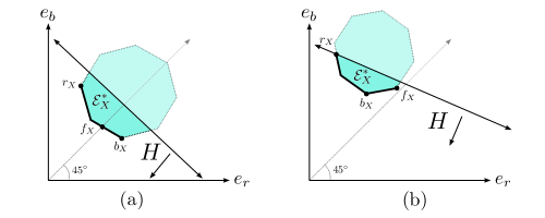
Figure 6. Depiction of an example input-design fairness-accuracy frontier for (a) a group-balanced covariate vector $X$ and (b) an $r$-skewed covariate vector $X$. In Panel (a), it is sufficient to check $r_{X},b_{X}\in H$ to determine whether the entire unconstrained fairness-accuracy frontier belongs to $H$. This condition is satisfied in the figure, so every designer can implement his favorite unconstrained outcome using input design. In Panel (b), it is sufficient to check whether $r_{X},f_{X}\in H$. This condition is failed in the figure, so some designer cannot implement his favorite unconstrained outcome using input design.

4.2. Excluding a Covariate

We turn next to the question of whether the optimal garbling may involve a complete ban on the use of a specific covariate. For example, there is an active debate regarding whether race should be a permitted input into clinical prediction algorithms (Vyas et al., 2020; Manski, 2022; Manski et al., 2022), and the University of California university system recently excluded consideration of standardized test scores from their admissions decisions.

Since the designer and agent have (potentially) misaligned preferences, banning an input can be optimal. But for two important classes of inputs, we will show that bans are strictly worse for all designers in the following sense:

Definition 4.4.

Say that excluding covariate vector $X^{\prime}$ over $X$ uniformly worsens the (input design) frontier if every point in $\mathcal{F}^{*}_{X}$ is FA-dominated by a point in $\mathcal{F}^{*}_{X,X^{\prime}}$.

To interpret this condition, recall that $\mathcal{F}^{*}_{X}$ is the frontier of error pairs that can be implemented by some garbling of $X$, while $\mathcal{F}^{*}_{X,X^{\prime}}$ is the frontier of error pairs that can be implemented by some garbling of $(X,X^{\prime})$. So any point that belongs to $\mathcal{F}^{*}_{X,X^{\prime}}$ but not to $\mathcal{F}^{*}_{X}$ can only be implemented if the garbling chosen by the designer includes information about $X^{\prime}$. When excluding $X^{\prime}$ over $X$ uniformly worsens the frontier, no designer’s optimal garbling excludes $X^{\prime}$, and so a ban on $X^{\prime}$ is not optimal for any designer with FA-preferences.

4.2.1. Excluding Group Identity

First let $X^{\prime}=G$, so that the comparison is between the frontier implemented by garblings of $X$ and the frontier implemented by garblings of $(X,G)$. The property of group balance (suitably strengthened) turns out to be critical for whether exclusion of $G$ uniformly worsens the frontier.

Definition 4.5.

Say that $X$ is strictly group-balanced if $e_{r}<e_{b}$ at $r_{X}$ and $e_{b}<e_{r}$ at $b_{X}$.

Relative to group-balance, strict group-balance rules out covariate vectors $X$ for which $r_{X}=b_{X}=f_{X}$.

Proposition 4.2.

Suppose $r_{X},b_{X}\in H$. Then, excluding $G$ over $X$ uniformly worsens the frontier if and only if $X$ is strictly group-balanced.

To show this result, we first demonstrate that the minimal (and maximal) feasible error for both groups is the same given $X$ and given $(X,G)$. Geometrically, this means that the feasible set given $(X,G)$ is the smallest rectangle containing the feasible set given $X$. When $X$ is group-balanced, then $\mathcal{F}^{*}_{X}$ is characterized by Part (a) of Theorem 3.1 while $\mathcal{F}^{*}_{X,G}$ is characterized by Proposition 3.1 (using the equivalence in Proposition 4.1 for both cases). As depicted in Panel (a) of Figure 7, the fairness-accuracy frontier given $X$ does not intersect with the frontier given $(X,G)$, so every point on the frontier given $X$ is FA-dominated by a point on the frontier given $(X,G)$. On the other hand, when $X$ is group-skewed, the two frontiers necessarily overlap as depicted in Panel (b).

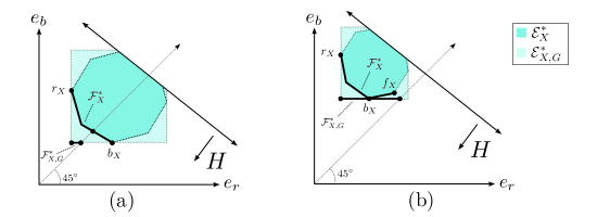
Figure 7. (a) $X$ is strictly group-balanced and excluding $G$ over $X$ uniformly worsens the input-design frontier; (b) $X$ is $r$-skewed and excluding $G$ over $X$ does not uniformly worsen the input-design frontier.

Proposition 4.2 says that so long as $X$ is strictly group-balanced, then every designer is made strictly better off if given access to group identity. That is, every designer can find a way of combining the information in $G$ and $X$—for example, by adding noise to $X$ for individuals in one group but not the other—which induces the agent to choose an algorithm that the agent would not have chosen given any garbling of $X$ alone. In contrast, if $X$ is not strictly group-balanced, then there is at least one designer for whom no garbling of $(X,G)$ strictly improves over garblings of $X$. For example, we see in Panel (b) of Figure 7 that the Rawlsian designer’s payoffs is not improved by access to $G$.

Our results complement papers such as Chan and Eyster (2003) and Rambachan et al. (2021), which compare choice between decision rules based on $(X,G)$ to choice between decision rules based on $X$ alone. Our property of a uniform worsening of the frontier does not in general rank the information policy of fully revealing $X$ versus fully revealing $(X,G)$. That is, it may be that excluding $G$ over $X$ uniformly worsens the frontier, but the designer’s payoff is higher from revealing $X$ than from revealing $(X,G)$.

Nevertheless, our result relates to and builds on previous findings that disparate treatment (use of different rules for individuals in different groups) may be necessary to preclude disparate impact (disparate harms across groups). Specifically, Proposition 4.2 implies that to reduce disparate impact, it may be necessary to impose information policies that are asymmetric across groups. Interestingly, this may not involve sending $G$ as an input, so the algorithm can be formally group-blind (thus not exhibiting disparate treatment). Nevertheless, if we consider the total procedure—taking into account both information design and algorithm design—then two individuals who are otherwise identical but belong to different groups may receive different distributions of outcomes. This distinction brings up an interesting question regarding how disparate treatment should be conceptualized in settings where both information design and algorithm design are present.

4.2.2. Excluding a Covariate When Group Identity is Known

Next compare the frontier implemented by garblings of $(X,G)$ with the frontier implemented by garblings of $(X,G,X^{\prime})$, where $X$ and $X^{\prime}$ are arbitrary covariate vectors.

Definition 4.6.

Say that $X^{\prime}$ is decision-relevant over $X$ for group $g$ if there are realizations $(x,x^{\prime})$ and $(x,\tilde{x}^{\prime})$ of $(X,X^{\prime})$ that have strictly positive probability conditional on $G=g$, where

$$\{1\}=\operatorname*{arg\,min}_{d\in\mathcal{D}}\mathbb{E}[\ell(d,Y)\mid(X,X^{\prime},G)=(x,x^{\prime},g)]$$

while

$$\{0\}=\operatorname*{arg\,min}_{d\in\mathcal{D}}\mathbb{E}[\ell(d,Y)\mid(X,X^{\prime},G)=(x,\tilde{x}^{\prime},g)].$$

This weak condition requires only that there is some individual in group $g$ for whom the decision that maximizes (expected) accuracy is different given $X$ and given $(X,X^{\prime})$. For example, if $X^{\prime}$ is a test score and $X$ is high school GPA, then $X^{\prime}$ is decision-relevant for group $g$ if taking the test score into consideration reverses the admission decision for at least one individual in group $g$ relative to the decision based on GPA alone. College entrance exams satisfy this property (Systemwide Academic Senate, 2020).

Proposition 4.3.

Choose arbitrary covariate vectors $X$ and $X^{\prime}$.

• If $(X,G)$ is $g$-skewed, then excluding $X^{\prime}$ over $(X,G)$ uniformly worsens the frontier if and only if $X^{\prime}$ is decision-relevant over $X$ for group $g^{\prime}\neq g$.

• If $(X,G)$ is group-balanced, then excluding $X^{\prime}$ over $(X,G)$ uniformly worsens the frontier if and only if $X^{\prime}$ is decision-relevant over $X$ for both groups.

When $X^{\prime}$ is decision-relevant over $X$ for the disadvantaged group, then the minimal feasible error for that group given $(X,G,X^{\prime})$ is strictly lower than the minimal feasible error given $(X,G)$ only. So the fairness-accuracy frontier is pushed towards the origin (either downwards or towards the left), as in Panel (a) of Figure 8. On the other hand, when $X^{\prime}$ is not decision-relevant over $X$ for the disadvantaged group, then the new fairness-accuracy frontier must remain a line that overlaps with the previous frontier (see Panel (b) of Figure 8), so there is some FA preference for which excluding $X^{\prime}$ is at least weakly (and possibly strictly) worse. This yields part (a) of the result. Part (b) pertains to a knife-edge case: If $(X,G)$ is group-balanced then the minimal feasible error is the same for both groups. For a uniform worsening of the frontier to occur, access to $X^{\prime}$ over $X$ must reduce the minimal feasible error for both groups.

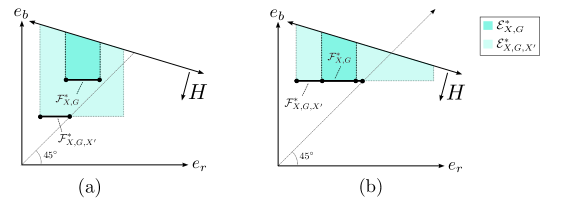
Figure 8. (a) Example in which $X^{\prime}$ is decision-relevant for group $b$, and excluding $X^{\prime}$ uniformly worsens the frontier; (b) Example in which $X^{\prime}$ is not decision-relevant for group $b$, and excluding $X^{\prime}$ does not uniformly worsen the frontier.

We can apply Proposition 4.3 to the question of whether to ban test scores in college admissions decisions. Our result suggests that so long as group identities are permissible inputs for college admission decisions, then excluding test scores is welfare-reducing for all designers with the ability to garble available covariates. On the other hand, if group identity is not permitted as an input into college admissions decisions, then a sufficiently fairness-minded designer may find it optimal to completely exclude test scores. With regards to the pending Supreme Court case Students for Fair Admissions, Inc. v. President and Fellows of Harvard College, our result suggests that if affirmative action is banned nationwide, then universities with certain FA preferences will have more reason to ban the use of test scores in admissions decisions.

While our framework abstracts away from many important features of the college admissions process—including access to testing (Garg et al., 2021) and test-optional admissions (Dessein et al., 2022))—the link between the availability of group identity and the value of additional information, such as test scores, is one that we believe holds more generally. The crucial point is that when group identity is available, the designer can tailor how the additional information is used for each group separately. For example, the designer could selectively report test scores only for standout students in the disadvantaged group. In this sense, access to group identity has a positive spillover effect for the value of other covariates, guaranteeing that there is some (possibly group-dependent) garbling of the other information that aligns the agent and designer’s incentives.

We conclude with the following simple example, which illustrates the contrast between access to an auxiliary covariate $X^{\prime}$ alone versus access to the pair $(X^{\prime},G)$.

Example 13.

Suppose $\mathcal{Y}=\{0,1\}$ and $Y$ and $G$ are independently and uniformly distributed, i.e., $\mathbb{P}(Y=y,G=g)=1/4$ for any $y\in\{0,1\}$ and $g\in\{r,b\}$. Let $X$ be a null signal; that is, $X=x_{0}$ with probability one. Further let $X^{\prime}$ be a binary signal with the following conditional probabilities $\mathbb{P}(X^{\prime}\mid Y,G)$:

$$\begin{array}[]{ccc}&X^{\prime}=1&X^{\prime}=0\\ Y=1&1&0\\ Y=0&0&1\end{array}\quad\quad\quad\begin{array}[]{ccc}&X^{\prime}=1&X^{\prime}=0\\ Y=1&0.6&0.4\\ Y=0&0.4&0.6\end{array}$$

$$G=r\hskip 142.26378ptG=b$$

Thus, $X^{\prime}$ is perfectly informative about the individuals in group $r$, and imperfectly informative about those in group $b$. Suppose the loss function is $\ell(d,y)=\mathbbm{1}(d\neq y)$, and the agent is Utilitarian ($\alpha_{r}=p_{r}=1/2$ and $\alpha_{b}=p_{b}=1/2$).

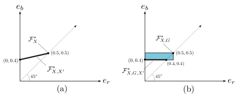
Figure 9. (a) A comparison of the input-design fairness-accuracy frontiers given $X$ versus given $(X,X^{\prime})$; (b) A comparison of the input-design fairness-accuracy frontiers given $(X,G)$ versus given $(X,G,X^{\prime})$

.

The input-design feasible set given $X$ only is the singleton $\{(0.5,0.5)\}$, which delivers a payoff of 0 to the Egalitarian designer. But if the designer chooses any nontrivial garbling of $(X,X^{\prime})$, the agent will use what he learns about $X^{\prime}$ to maximize aggregate accuracy. Since this information is inevitably more informative about group $r$ than about group $b$, conditioning decisions on this information increases the gap between the two group errors, reducing the designer’s payoff. So it is strictly optimal for the designer to exclude all information about $X^{\prime}$. In more detail, the fairness-accuracy frontier given $(X,X^{\prime})$ is the line segment connecting $(0,0.4)$ with $(0.5,0.5)$ (see Panel (a) of Figure 9), and any nontrivial garbling of $(X,X^{\prime})$ leads to a point on this frontier that is different from $(0.5,0.5)$, yielding a strictly negative payoff for the designer.

In contrast, Panel (b) of Figure 9 demonstrates the comparison between the fairness-accuracy frontiers $\mathcal{F}^{*}_{X,G}$ and $\mathcal{F}^{*}_{X,G,X^{\prime}}$. Here we see that the Egalitarian designer is able to achieve the superior outcome $(0.4,0.4)$ by choosing an appropriate garbling of $(X,G,X^{\prime})$. Thus while making information about $X^{\prime}$ available to the agent is strictly harmful for the designer when group identity is not available, this ceases to be true once the designer can condition the garbling of $X^{\prime}$ on $G$.

5. Extensions

5.1. Different loss functions for evaluating fairness and accuracy.

When defining the partial order $>_{FA}$, we used the same loss function to evaluate both accuracy and fairness. This is suitable, for example, for healthcare decisions where both the healthcare provider (designer) and patients agree that more accurate decisions are better, and so fairness can be reasonably evaluated as the disparity in accuracy across groups. In other cases where the subjects’ utility function is different from the designer’s, policymakers sometimes evaluate accuracy using one loss function and fairness using another. For example, if the algorithm guides hiring decisions, then fairness may be evaluated as the difference in hiring rates across groups, even while accuracy is evaluated based on whether suitable candidates are hired. In Appendix O.1 we develop a more general version of our framework that allows for different loss functions, and extends Theorem 3.1 and Corollary 3.1 under a generalization of group-balance.

5.2. Beyond absolute difference for evaluating fairness.

Our main analysis assumes that (un)fairness is evaluated according to the absolute difference of errors between the two groups, i.e. $|e_{r}-e_{b}|$. A natural extension is to consider $|\phi(e_{r})-\phi(e_{b})|$ where $\phi$ is some continuous strictly increasing function. For instance, if $\phi$ is $\log$, then this corresponds to evaluating fairness using the ratio of errors rather than their difference. Theorem 3.1 holds for any such $\phi$ with the fairness optimal point $f_{X}$ suitably defined. We further demonstrate that the frontier becomes larger (smaller) whenever $\phi$ is concave (convex). Thus, for example, evaluating fairness using ratios instead of absolute difference results in a larger frontier, although the qualitative properties of this frontier are unchanged.

5.3. Other agent preferences in the input design problem.

Section 4 considers misaligned incentives between a designer controlling inputs and an agent setting the algorithm. There, we assume that the agent cares about accuracy and prefers for both group errors to be lower. In Appendix O.4, we consider what happens when this misalignment is more extreme and the agent is adversarial (i.e. negatively biased) towards one of the two groups, preferring that group’s error to be higher. We generalize several results from Section 4 and show that even if the agent is negatively biased, it can still be optimal for the designer to provide information about group identity (so long as the bias is not too extreme).

Two other potential generalizations would permit the agent and designer to have different loss functions, or permit the agent to care about fairness. In both cases, the set of points that the agent prefers over the prior (what we defined to be $H$) is no longer a halfspace from the designer’s perspective. Moreover, non-linearities in the agent’s objective function imply that the agent’s ex-ante and ex-post problems may be different, and so it is relevant whether the agent commits to the algorithm or chooses the decision after the realization of the garbling. We consider these problems beyond the scope of the present paper, and leave them as open questions for future work.

5.4. Capacity constraints.

In our main model, we allow the designer unconstrained choice of any algorithm. In a few of the applications of interest, there may be an additional capacity constraint on the algorithm, e.g., if only a fixed number of students can be admitted in admissions decisions. One way to formulate a capacity constraint is a restriction on the ex-ante probability of assignment of decision $d=1$ (e.g., admit). In this case, the set of error pairs satisfying the constraint can be shown to be a convex set, so the feasible set is simply the intersection between the feasible set (as we have defined) and the convex set of error pairs that satisfy this capacity constraint. Our Theorem 3.1 then applies for this new feasible set, although the fairness-accuracy frontier as characterized in Proposition 3.1 may no longer be a horizontal line.

5.5. More than two groups or two decisions.

We have assumed that there are two groups $\mathcal{G}=\{r,b\}$. Some of our results, such as Proposition 4.1, can be shown to directly extend for any finite $\mathcal{G}$. However, in order to extend our other results, we would first have to specify a definition of fairness for multiple groups. One possible generalization of the FA-dominance relationship is to say that a vector of group errors $(e_{g})_{g\in\mathcal{G}}$ FA-dominates another vector $(e_{g}^{\prime})_{g\in\mathcal{G}}$ if $e_{g}\leq e_{g}^{\prime}$ for every group $g$, and also $|e_{g}-\frac{1}{|\mathcal{G}|}\sum_{g\in\mathcal{G}}e_{g}|\leq|e_{g}^{\prime}-\frac{1}{|\mathcal{G}|}\sum_{g\in\mathcal{G}}e_{g}^{\prime}|$ for every $g\in\mathcal{G}$, with at least one inequality holding strictly. That is, fairness is improved if each group’s error is closer to the average group error. We expect our characterization in Theorem 3.1 to extend qualitatively in this case.

We have also assumed that there are two decisions $\mathcal{D}=\{0,1\}$. All of our results in Section 3 about the unconstrained problem directly extend for any finite $\mathcal{D}$. However, Lemma 4.1 (the relationship between the input-design fairness-accuracy frontier and the unconstrained fairness-accuracy frontier) relies on the assumption of a binary decision. We leave a characterization of the input design frontier for this more general case to future work.

Appendix A Proofs for Main Results

A.1. Characterization of the Feasible Set

Lemma A.1.

$\mathcal{E}_{X}$ is a closed and convex polygon.

Proof.

Given algorithm $a$, we slightly abuse notation to let $a(x)$ denote the probability of choosing decision $d=1$ at covariate vector $x$. We further let $x_{y,g}$ denote the conditional probability that $Y=y$ and $G=g$ given $X=x$. Finally, let $p_{x}$ denote the probability of $X=x$. Then the group errors can be written as follows:

$$e_{g}(a) =\mathbb{E}\left[a\left(X\right)\ell\left(1,Y\right)+\left(1-a\left(X\right)\right)\ell\left(0,Y\right)\mid G=g\right]$$

$$=\sum_{x}\left(a\left(x\right)\sum_{y}\frac{x_{y,g}}{p_{g}}\ell\left(1,y\right)+\left(1-a\left(x\right)\right)\sum_{y}\frac{x_{y,g}}{p_{g}}\ell\left(0,y\right)\right)\cdot p_{x},$$

where $p_{g}$ is the prior probability that $G=g$. The set of all feasible errors is given by

$$\mathcal{E}_{X}=\left\{\left(e_{r}\left(a\right),e_{b}\left(a\right)\right)\text{ : }a:\mathcal{X}\rightarrow[0,1]\right\}.$$

If we let

$$E\left(x\right):= \left\{\lambda\left(\sum_{y}\frac{x_{y,r}}{p_{r}}\ell\left(1,y\right),\sum_{y}\frac{x_{y,b}}{p_{b}}\ell\left(1,y\right)\right)\right.$$

$$\left.\quad\quad\quad+\left(1-\lambda\right)\left(\sum_{y}\frac{x_{y,r}}{p_{r}}\ell\left(0,y\right),\sum_{y}\frac{x_{y,b}}{p_{b}}\ell\left(0,y\right)\right)\text{ : }\lambda\in\left[0,1\right]\right\}$$

represent a line segment in $\mathbb{R}^{2}$, then we see that $\mathcal{E}_{X}=\sum_{x\in\mathcal{X}}E\left(x\right)\cdot p_{x}.$ This is a (weighted) Minkowski sum of line segments, which must be a closed and convex polygon. ∎

A.2. Proof of Theorem 3.1

First observe that the FA frontier must be part of the boundary of the feasible set $\mathcal{E}_{X}$, because any interior point $(e_{r},e_{b})$ is FA-dominated by $(e_{r}-\epsilon,e_{b}-\epsilon)$ which is feasible when $\epsilon$ is small.

Consider the group-balanced case, where $r_{X}$ lies weakly above the 45-degree line and $b_{X}$ lies weakly below. If $r_{X}=b_{X}$, then this point simultaneously achieves minimal error for both groups, as well as minimal unfairness since it must be on the 45-degree line. In this case it is clear that the fairness-accuracy frontier consists of that single point, which FA-dominates every other feasible point. Another degenerate case is when the entire feasible set $\mathcal{E}_{X}$ consists of the line segment $r_{X}b_{X}$. Here again it is easy to see that the entire line segment is FA-undominated, and the result also holds.

Next we show that the upper boundary of $\mathcal{E}_{X}$ connecting $r_{X}$ to $b_{X}$ (excluding $r_{X}$ and $b_{X}$) is FA-dominated. One possibility is that the upper boundary consists entirely of the line segment $r_{X}b_{X}$. Take any point $q$ on this line segment, and through it draw a line parallel to the 45-degree line. Then this line intersects the boundary of $\mathcal{E}_{X}$ at another point $q^{\prime}$ (otherwise we return to the degenerate case above). By our current assumption about the upper boundary, this point $q^{\prime}$ must be strictly below the line segment $r_{X}b_{X}$. It follows that $q^{\prime}$ reduces both group errors compared to $q$, by the same amount. Thus $q^{\prime}>_{FA}q$. If instead the upper boundary is strictly above the line segment $r_{X}b_{X}$, then through any such boundary point $q$ we can still draw a line parallel to the 45-degree line. But now let $q^{*}$ be the intersection of this line with the extended line $r_{X}b_{X}$. If $q^{*}$ lies between $r_{X}$ and $b_{X}$, then it is feasible and FA-dominates $q$ because both groups’ errors are reduced by the same amount. Suppose instead that $q^{*}$ lies on the extension of the ray $b_{X}r_{X}$ (the other case being symmetric), then we claim that $r_{X}$ itself FA-dominates $q$. Indeed, by definition $q$ must have weakly larger $e_{r}$ than $r_{X}$. And because in this case $q^{*}$ is farther away from the 45-degree line than $r_{X}$ (this is where we use the assumption that $r_{X}$ is already above that line), $q^{*}$ and thus $q$ also induce strictly larger group error difference $e_{b}-e_{r}$ than $r_{X}$. Hence $q$ has larger $e_{r}$, $e_{b}-e_{r}$ as well as $e_{b}$ when compared to $r_{X}$, as we desire to show.

To complete the proof for the group-balanced case, we need to show that the lower boundary connecting $r_{X}$ to $b_{X}$ is not FA-dominated. $r_{X}$ (and symmetrically $b_{X}$) cannot be FA-dominated, because it minimizes $e_{r}$ and conditional on that further minimizes $e_{b}$ uniquely. Take any other point $q$ on the lower boundary. If $q$ lies on the line segment $r_{X}b_{X}$, then the lower boundary consists entirely of this line segment. In this case $q$ minimizes a certain weighted average of group errors $\alpha e_{r}+\beta e_{b}$ across all feasible points, where $\alpha,\beta>0$ are such that the vector $(\alpha,\beta)$ is orthogonal to the line segment $r_{X}b_{X}$ (which necessarily has a negative slope). Any such point $q$ cannot be FA-dominated, since a dominant point would have smaller $\alpha e_{r}+\beta e_{b}$. Finally suppose $q$ is a boundary point strictly below the line segment $r_{X}b_{X}$. Then it minimizes some weighted sum of group errors $\alpha e_{r}+\beta e_{b}$, and it will suffice to show that the weights $\alpha,\beta$ must be positive. Indeed, $\alpha,\beta\leq 0$ cannot happen because $q$ induces smaller $e_{r},e_{b}$ than $q^{*}$ ($q^{*}$ defined in the same way as before but now to the top-right of $q$) and thus larger $\alpha e_{r}+\beta e_{b}$. $\alpha>0\geq\beta$ cannot happen because $q$ induces larger $e_{r}$ and smaller $e_{b}$ than $r_{X}$, and thus also larger $\alpha e_{r}+\beta e_{b}$. Symmetrically $\beta>0\geq\alpha$ cannot happen either. So we indeed have $\alpha,\beta>0$, which implies that $q$ is FA-undominated. This proves the result for the group-balanced case.

This argument can be adapted to the group-skewed case as follows. Suppose $X$ is $r$-skewed, so that $r_{X}$ and $b_{X}$ are both above the 45-degree line. To show that the upper boundary connecting $r_{X}$ to $f_{X}$ is FA-dominated, we choose any boundary point $q$ and (similar to the above) let $q^{*}$ be on the extended line $r_{X}f_{X}$ such that $qq^{*}$ is parallel to the 45-degree line. If $q^{*}$ is on the line segment $r_{X}f_{X}$ then it is a feasible point that FA-dominates $q$. If $q^{*}$ lies on the extension of the ray $f_{X}r_{X}$, then as before it can be shown that $r_{X}>_{FA}q$. Finally if $q^{*}$ lies on the extension of the ray $r_{X}f_{X}$, then it must be the case that $f_{X}$ lies on the 45-degree line (otherwise it will not minimize $|e_{r}-e_{b}|$ as defined). In this case $q$ is a point that is below the 45-degree line, but also above the extended line $b_{X}f_{X}$ by convexity of the feasible set. Since $f_{X}$ already has larger $e_{b}$ than $b_{X}$, we see that $q$ must in turn have larger $e_{b}$ than $f_{X}$. But then it follows that $q$ is FA-dominated by $f_{X}$ as it has larger $e_{b}$, larger $e_{r}-e_{b}$ (being below the 45-degree line where $f_{X}$ belongs to), and thus also larger $e_{r}$.

It remains to show that the lower boundary connecting $r_{X}$ to $f_{X}$ is FA-undominated. By essentially the same argument, we know that the lower boundary from $r_{X}$ to $b_{X}$ is FA-undominated. As for the lower boundary from $b_{X}$ to $f_{X}$, note that if some point $q$ here is FA-dominated by another boundary point $\widehat{q}$, then $\widehat{q}$ must induce smaller $|e_{b}-e_{r}|$. Since $e_{b}-e_{r}$ is positive at $q$, this means that $\widehat{q}$ induces smaller $e_{b}-e_{r}$ than $q$, without the absolute value applied to the difference. So either $\widehat{q}$ lies on the lower boundary from $q$ to $f_{X}$, or $\widehat{q}$ belongs to the other side of the 45-degree line (i.e., below it). Either way the alternative point $\widehat{q}$ must be farther away from $b_{X}$ than $q$ on the lower boundary, so that by convexity $\widehat{q}$ lies above the extended line $b_{X}q$. Given that $q$ already has larger $e_{b}$ than $b_{X}$, this implies that $\widehat{q}$ has even larger $e_{b}$ than $q$. Hence $\widehat{q}$ cannot in fact FA-dominate $q$, completing the proof.

A.3. Proof of Corollary 3.1

Suppose $X$ is group-balanced, then by Theorem 3.1 the fairness-accuracy frontier is the lower boundary from $r_{X}$ to $b_{X}$. Let $m_{X}$ be the group error pair that consists of the $e_{r}$ in $r_{X}$ and the $e_{b}$ in $b_{X}$ (geometrically, $m_{X}$ is such that the line segments $r_{X}m_{X}$ and $b_{X}m_{X}$ are parallel to the axes). Then because $r_{X}$ and $b_{X}$ have respectively minimal group errors in the feasible set, and because we are considering the lower boundary, any point on this lower boundary $\mathcal{F}_{X}$ must belong to the triangle with vertices $r_{X},b_{X}$ and $m_{X}$. This implies by convexity that each edge of this lower boundary has a negative slope (just note that the first and final edges must have negative slopes). Because of this, if we start from $r_{X}$ and traverse along this lower boundary, it must be the case that $e_{r}$ continuously increases while $e_{b}$ continuously decreases. Thus in the group-balanced case there does not exist any strong fairness-accuracy conflict along the fairness-accuracy frontier.

On the other hand, suppose $X$ is $r$-skewed. Then we claim that $b_{X}$ and $f_{X}$ (which are assumed to be distinct) present a strong fairness-accuracy conflict. Indeed, by assumption of $r$-skewness, $b_{X}$ is weakly above the 45-degree line. $f_{X}$ must also be weakly above the 45-degree line because otherwise it would be less fair compared to the point on the line segment $b_{X}f_{X}$ that also belongs to the 45-degree line. Thus, the fact that $f_{X}$ is weakly more fair than $b_{X}$ implies that $f_{X}$ entails smaller $e_{b}-e_{r}$ than $b_{X}$. By definition of $b_{X}$, $f_{X}$ entails larger $e_{b}$ than $b_{X}$. Combining the above two observations, we know that $f_{X}$ also entails larger $e_{r}$ than $b_{X}$. Hence $f_{X}$ induces larger group errors than $b_{X}$ for both groups, but reduces the difference in group errors. This is a strong fairness-accuracy conflict as we desire to show.

A.4. Proof of Proposition 3.1

We recall the proof of Lemma A.1, where we showed that the feasible set $\mathcal{E}_{X}$ can be written as $\sum_{x}E\left(x\right)\cdot p_{x}$, with $E(x)$ representing the line segment connecting the two points

$$\left(\sum_{y}\frac{x_{y,r}}{p_{r}}\ell\left(1,y\right),\sum_{y}\frac{x_{y,b}}{p_{b}}\ell\left(1,y\right)\right)$$

and

$$\left(\sum_{y}\frac{x_{y,r}}{p_{r}}\ell\left(0,y\right),\sum_{y}\frac{x_{y,b}}{p_{b}}\ell\left(0,y\right)\right)$$

where all notations are as defined in the proof of Lemma A.1.

If $X$ reveals $G$, then for each realization $x$, either $x_{y,r}=0$ for all $y$ or $x_{y,b}=0$ for all $y$. Thus each $E(x)$ is a horizontal or vertical line segment, implying that $\mathcal{E}_{X}$ must be a rectangle with $r_{X}=b_{X}$ being its bottom-left vertex.

Suppose without loss of generality that $r_{X}=b_{X}$ lies above the 45-degree line. If the rectangle $\mathcal{E}_{X}$ does not intersect the 45-degree line, then it is easy to see that $f_{X}$ must be the bottom-right vertex of $\mathcal{E}_{X}$. In this case the fairness-accuracy frontier is the entire bottom edge of the rectangle, which is a horizontal line segment. If instead the rectangle $\mathcal{E}_{X}$ intersects the 45-degree line, then $f_{X}$ is the intersection between the bottom edge of $\mathcal{E}_{X}$ and the 45-degree line. Again the fairness-accuracy frontier is the horizontal line segment from $r_{X}=b_{X}$ to $f_{X}$. This proves the result.

A.5. Proof of Proposition 3.2

We will show that $b_{X}=r_{X}$ under conditional independence, and the result then follows from Theorem 3.1. Recall from the proof of Lemma A.1 that

$$\mathcal{E}_{X}=\sum_{x\in\mathcal{X}}E\left(x\right)p_{x}$$

where

$$E\left(x\right)= \left\{\lambda\left(\sum_{y}\frac{x_{y,r}}{p_{r}}\ell\left(1,y\right),\sum_{y}\frac{x_{y,b}}{p_{b}}\ell\left(1,y\right)\right)\right.$$

$$\left.+\left(1-\lambda\right)\left(\sum_{y}\frac{x_{y,r}}{p_{r}}\ell\left(0,y\right),\sum_{y}\frac{x_{y,b}}{p_{b}}\ell\left(0,y\right)\right)\text{ : }\lambda\in\left[0,1\right]\right\}$$

Under conditional independence, $x_{y,g}=x_{y}x_{g}$ (with $x_{y}\equiv P(Y=y\mid X=x)$ and $x_{g}\equiv P(G=g\mid X=x)$) so we have

$$E\left(x\right)=\left\{\left(\lambda\sum_{y}x_{y}\ell\left(1,y\right)+\left(1-\lambda\right)\sum_{y}x_{y}\ell\left(0,y\right)\right)\left(\frac{x_{r}}{p_{r}},\frac{x_{b}}{p_{b}}\right)\text{\text{ : }$\lambda\in\left[0,1\right]$}\right\}$$

This means that for each realization $x\in\mathcal{X}$, the outcome that gives the lower error for group $r$ also gives the lower error for group $b$. In other words, when $\sum_{y}x_{y}\ell\left(1,y\right)\leq\sum_{y}x_{y}\ell\left(0,y\right)$, then the decision $d=1$ is optimal for both groups (and vice-versa if the inequality is reversed). Consider the following algorithm:

$$a\left(x\right)=\begin{cases}1&\text{if }\sum_{y}x_{y}\ell\left(1,y\right)\leq\sum_{y}x_{y}\ell\left(0,y\right)\\ 0&\text{if }\sum_{y}x_{y}\ell\left(1,y\right)>\sum_{y}x_{y}\ell\left(0,y\right)\end{cases}$$

This algorithm will deliver the lowest error for both groups and

$$(e_{r}\left(a\right),e_{b}\left(a\right))=r_{X}=b_{X}$$

as desired.

A.6. Proof of Lemma 4.1

We first characterize the input-design feasible set, and later study the input-design fairness-accuracy frontier. It is clear that regardless of what garbling the designer gives the agent, the agent’s payoff will be weakly better than what can be achieved under no information. Thus any error pair that is implementable by input-design must belong to the halfspace $H$. Such an error pair must also belong to the feasible set $\mathcal{E}_{X}$, so we obtain the easy direction $\mathcal{E}^{*}_{X}\subseteq\mathcal{E}_{X}\cap H$ in the lemma.

Conversely, we need to show that a feasible error pair $(e_{r},e_{b})\in\mathcal{E}_{X}$ that satisfies $\alpha_{r}e_{r}+\alpha_{b}e_{b}\leq e_{0}$ can be implemented by some garbling $T$. Consider a garbling $T$ that maps $X$ to $\Delta(\mathcal{D})$, with the interpretation that the realization of $T(x)$ is the recommended decision for the agent. If we abuse notation to let $a(x)$ denote the probability that the recommendation is $d=1$ at covariate vector $x$, then this algorithm $a$ needs to satisfy the following obedience constraint for $d=1$:

$$\sum_{y,g}\frac{\alpha_{g}}{p_{g}}\sum_{x}p_{x,y,g}\cdot a(x)\cdot\ell(1,y)\leq\sum_{y,g}\frac{\alpha_{g}}{p_{g}}\sum_{x}p_{x,y,g}\cdot a(x)\cdot\ell(0,y).$$

The above is just equation (4.1) adapted to the current setting with the observation that given the recommendation $T=1$, the conditional probability of $Y=y$ and $G=g$ is proportional to the recommendation probability $\sum_{x}p_{x,y,g}\cdot a(x)$, where we use $p_{x,y,g}$ as a shorthand for $\mathbb{P}(X=x,Y=y,G=g)$.

Let us rewrite the above displayed equation as

$$\sum_{x,y,g}p_{x,y,g}\frac{\alpha_{g}}{p_{g}}\cdot a(x)\ell(1,y)\leq\sum_{x,y,g}p_{x,y,g}\frac{\alpha_{g}}{p_{g}}\cdot a(x)\ell(0,y).$$

If we add $p_{x,y,g}\frac{\alpha_{g}}{p_{g}}(1-a(x))\ell(0,y)$ to each summand above, we obtain

(A.1) $$\sum_{x,y,g}p_{x,y,g}\frac{\alpha_{g}}{p_{g}}\cdot\left(a(x)\ell(1,y)+(1-a(x))\ell(0,y)\right)\leq\sum_{x,y,g}p_{x,y,g}\frac{\alpha_{g}}{p_{g}}\cdot\ell(0,y).$$

Now, the LHS above can be rewritten as $\sum_{x,y,g}p_{x,y,g}\frac{\alpha_{g}}{p_{g}}\cdot\mathbb{E}_{D\sim a(x)}[\ell(D,y)\mid X=x,Y=y,G=g]$, which is also equal to $\sum_{g}\alpha_{g}\cdot\mathbb{E}_{D\sim a(x)}[\ell(D,Y)\mid G=g]$. This is precisely the agent’s expected loss when following the designer’s recommended decisions.

On the other hand, the RHS in (A.1) can be seen to be the agent’s expected loss when taking the decision $d=0$ regardless of the designer’s recommendation. Thus, we deduce that the obedience constraint for the recommendation $d=1$ is equivalent to (A.1), which simply says that the agent’s payoff under the designer’s recommendation should be weakly better than the constant decision $d=0$ ignoring the recommendation. Symmetrically, the other obedience constraint for the recommendation $d=0$ is equivalent to the agent’s payoff being better than the constant decision $d=1$. Put together, these obedience constraints thus reduce to the requirement that the designer’s recommendation gives the agent a payoff that exceeds what can be achieved with no information.

For any error pair $(e_{r},e_{b})$ that is feasible under unconstrained design, we can construct a garbling $T$ that implements it by recommending the desired decision. If $(e_{r},e_{b})$ belongs to the halfspace $H$, then by the previous analysis we know that obedience is satisfied. Thus $(e_{r},e_{b})$ is implementable under input-design, showing that $\mathcal{E}_{X}\cap H=\mathcal{E}^{*}_{X}$ as desired.

Finally we turn to the fairness-accuracy frontier and argue that $\mathcal{F}^{*}_{X}=\mathcal{F}_{X}\cap H$. In one direction, if an error pair is FA-undominated in $\mathcal{E}_{X}$ and implementable under input design, then it is also FA-undominated in the smaller set $\mathcal{E}^{*}_{X}$. This proves $\mathcal{F}_{X}\cap H\subseteq\mathcal{F}^{*}_{X}$. In the opposite direction, suppose for contradiction that a certain point $(e_{r},e_{b})\in\mathcal{F}^{*}_{X}$ does not belong to $\mathcal{F}_{X}\cap H$. Since $\mathcal{F}^{*}_{X}\subseteq\mathcal{E}^{*}_{X}\subseteq H$, we know that $(e_{r},e_{b})$ must not belong to $\mathcal{F}_{X}$. Thus by definition of $\mathcal{F}_{X}$, $(e_{r},e_{b})$ is FA-dominated by some other error pair $(\widehat{e_{r}},\widehat{e_{b}})\in\mathcal{E}_{X}$. In particular, we must have $\widehat{e_{r}}\leq e_{r}$ and $\widehat{e_{b}}\leq e_{b}$, which implies $\alpha_{r}\widehat{e_{r}}+\alpha_{b}\widehat{e_{b}}\leq\alpha_{r}e_{r}+\alpha_{b}e_{b}\leq e_{0}$ (the first inequality uses $\alpha_{r},\alpha_{b}\geq 0$ and the second uses $(e_{r},e_{b})\in\mathcal{F}^{*}_{X}\subseteq\mathcal{E}^{*}_{X}$). It follows that the FA-dominant point $(\widehat{e_{r}},\widehat{e_{b}})$ also belongs to $H$ and thus $\mathcal{E}^{*}_{X}$. But this contradicts the assumption that $(e_{r},e_{b})$ is FA-undominated in $\mathcal{E}^{*}_{X}$. Such a contradiction completes the proof.

A.7. Proof of Proposition 4.1

We now deduce Proposition 4.1 from Lemma 4.1. If $X$ is group-balanced, then by Theorem 3.1 we know that $\mathcal{F}_{X}$ is the part of the boundary of $\mathcal{E}_{X}$ that connects $r_{X}$ to $b_{X}$ from below. Clearly, $\mathcal{F}^{*}_{X}=\mathcal{F}_{X}$ can only hold if $r_{X},b_{X}\in\mathcal{F}^{*}_{X}\subseteq H$, so we focus on the “if” direction of the result. Suppose $r_{X},b_{X}\in H$, then we claim that the entire lower boundary of $\mathcal{E}_{X}$ from $r_{X}$ to $b_{X}$ belongs to $H$. Indeed, let $m_{X}$ be the point that has the same $e_{r}$ as $r_{X}$ and the same $e_{b}$ as $b_{X}$. Geometrically, $m_{X}$ is such that the line segments $m_{X}r_{X}$ and $m_{X}b_{X}$ are parallel to the axes. Because $r_{X},b_{X}$ have respectively minimal group errors in the feasible set $\mathcal{E}_{X}$, and because we are considering the lower boundary, any point on this lower boundary $\mathcal{F}_{X}$ must belong to the triangle with vertices $r_{X},b_{X}$ and $m_{X}$. Since $r_{X},b_{X},m_{X}$ all belong to the halfspace $H$ ($m_{X}\in H$ because the agent’s payoff weights $\alpha_{r},\alpha_{b}$ are non-negative), we deduce that $\mathcal{F}_{X}\subseteq H$. Hence whenever $r_{X},b_{X}\in H$, we have by Lemma 4.1 that $\mathcal{F}^{*}_{X}=\mathcal{F}_{X}\cap H=\mathcal{F}_{X}$. This argument proves Proposition 4.1 in the group-balanced case.

Suppose instead that $X$ is $r$-skewed (a symmetric argument applies to the $b$-skewed case). To generalize the above argument, we need to show that whenever $r_{X},f_{X}$ belong to $H$, then so does the entire lower boundary connecting these points. To see this, note that by the definition of $b_{X}$ and $f_{X}$, the lower boundary connecting these two points consists of positively sloped edges. So across all points on this part of the lower boundary, $f_{X}$ maximizes $\alpha_{r}e_{r}+\alpha_{b}e_{b}$. Thus the assumption $f_{X}\in H$ implies that the lower boundary from $b_{X}$ to $f_{X}$ belongs to $H$. In particular $b_{X}\in H$, which together with $r_{X}\in H$ implies that the lower boundary from $r_{X}$ to $b_{X}$ also belongs to $H$ (by the same argument as in the group-balanced case before). Hence the entire lower boundary from $r_{X}$ to $f_{X}$ belongs to $H$, as we desire to show.

A.8. Proof of Proposition 4.2

We first present a simple lemma which conveniently restates the property of “uniform worsening of frontier”:

Lemma A.2.

Excluding covariate $X^{\prime}$ over $X$ uniformly worsens the frontier if and only if $\mathcal{F}^{*}_{X}$ does not intersect with $\mathcal{F}^{*}_{X,X^{\prime}}$.

The proof of this lemma is straightforward: If there exists a point in $\mathcal{F}^{*}_{X}$ that also belongs to $\mathcal{F}^{*}_{X,X^{\prime}}$, then this point is not FA-dominated by any point in $\mathcal{F}^{*}_{X,X^{\prime}}$, so that the frontier does not uniformly worsen when excluding $X^{\prime}$. On the other hand, suppose no point in $\mathcal{F}^{*}_{X}$ belongs to $\mathcal{F}^{*}_{X,X^{\prime}}$. Note that any point in $\mathcal{F}^{*}_{X}$ is implementable via a garbling of $X$ and thus implementable via a garbling of $X,X^{\prime}$. Thus any such point belongs to $\mathcal{E}^{*}_{X,X^{\prime}}$, and since it is not FA-optimal in this set, it must be FA-dominated by some FA-optimal point in this (compact) set. In this case we do have uniform worsening of the frontier, as we desire to show.

Below we use Lemma A.2 to deduce Proposition 4.2. The key observation is that whether or not $G$ is excluded does not affect the minimal (or maximal) feasible error for either group. This is because if we want to minimize the error of a particular group $g$ using an algorithm that depends on $X$, then we essentially condition on $G=g$ anyways.

With this observation, suppose $X$ is strictly group-balanced. Then $r_{X}$ lies strictly above the 45-degree line and $b_{X}$ lies strictly below. Since we assume $r_{X},b_{X}\in H$, Proposition 4.1 tells us that the input-design fairness-accuracy frontier $\mathcal{F}^{*}_{X}$ is the same as the unconstrained fairness-accuracy frontier $\mathcal{F}_{X}$, and by Theorem 3.1 this frontier is the lower boundary of the feasible set $\mathcal{E}_{X}$ connecting $r_{X}$ to $b_{X}$. By Lemma A.2, we just need to show that in this case the lower boundary of $\mathcal{E}_{X}$ from $r_{X}$ to $b_{X}$ does not intersect with the input-design fairness-accuracy frontier $\mathcal{F}^{*}_{X,G}$ given $(X,G)$. To characterize the latter frontier, let $m_{X}=r_{X,G}=b_{X,G}$ denote the error pair that has the same $e_{r}$ as $r_{X}$ and the same $e_{b}$ as $b_{X}$. Without loss of generality assume $m_{X}$ lies weakly above the 45-degree line. Then from Proposition 3.1 we know that the unconstrained fairness-accuracy frontier $\mathcal{F}_{X,G}$ is the horizontal line segment from $m_{X}$ to $f_{X,G}$. This point $f_{X,G}$ is the intersection between the line segment $m_{X}b_{X}$ and the 45-degree line (here we use the fact that $m_{X}$ lies above the 45-degree line and $b_{X}$ lies below). As $b_{X}\in H$, the points $m_{X}$ and $f_{X,G}$ also belong to $H$ because they have equal $e_{b}$ and smaller $e_{r}$ compared to $b_{X}$. Hence the input-design fairness-accuracy frontier $\mathcal{F}^{*}_{X,G}$ is also the line segment from $m_{X}$ to $f_{X,G}$. To see that this horizontal line segment does not intersect the boundary of $\mathcal{E}_{X}$ from $r_{X}$ to $b_{X}$, just note that $b_{X}$ is the only point on that boundary with the same (minimal) $e_{b}$ as any point on the horizontal line segment. But $b_{X}$ does not belong to that line segment because it is strictly below the 45-degree line. This proves the result when $X$ is strictly group-balanced.

Now suppose $X$ is not strictly group-balanced. Then $r_{X}$ and $b_{X}$ lie weakly on the same side of the 45-degree line, and without loss of generality let us assume they lie weakly above. It is still the case that the unconstrained fairness-accuracy frontier $\mathcal{F}_{X,G}$ is the horizontal line segment from $m_{X}$ to $f_{X,G}$. But in the current setting $f_{X,G}$ must be weakly closer to the 45-degree line than $b_{X}$, which means that $b_{X}$ now lies in between $m_{X}$ and $f_{X,G}$. In other words, $b_{X}\in\mathcal{F}_{X}$ and $b_{X}\in\mathcal{F}_{X,G}$. But by assumption, $b_{X}$ also belongs to $H$. So Lemma 4.1 tells us that $b_{X}$ belongs to the input-design fairness-accuracy frontiers $\mathcal{F}^{*}_{X}$ and $\mathcal{F}^{*}_{X,G}$. This shows that the two frontiers $\mathcal{F}^{*}_{X}$ and $\mathcal{F}^{*}_{X,G}$ intersect, which completes the proof by Lemma A.2.

A.9. Proof of Proposition 4.3

Let $\underline{e}_{g}=\min\{e_{g}\mid e\in\mathcal{E}_{X,G}\}$ and $\overline{e}_{g}=\max\{e_{g}\mid e\in\mathcal{E}_{X,G}\}$ be the minimal and maximal feasible errors for group $g$ given covariate vector $(X,G)$, and define $\underline{e}^{*}_{g}=\min\{e_{g}\mid e\in\mathcal{E}_{X,G,X^{\prime}}\}$ and $\overline{e}^{*}_{g}=\max\{e_{g}\mid e\in\mathcal{E}_{X,G,X^{\prime}}\}$ to be the corresponding quantities given $(X,G,X^{\prime})$. The following lemma says that additional access to $X^{\prime}$ reduces the minimal feasible error for group $g$ relative to $(X,G)$ if and only if $X^{\prime}$ is decision-relevant over $X$ for group $g$.

Lemma A.3.

$\underline{e}^{*}_{g}<\underline{e}_{g}$ if $X^{\prime}$ is decision-relevant over $X$ for group $g$, and $\underline{e}^{*}_{g}=\underline{e}_{g}$ if it is not.

Proof.

Let $a_{g}:\mathcal{X}\rightarrow\{0,1\}$ be any strategy mapping each realization of $X$ into an optimal outcome for group $g$, i.e.,

$$a_{g}(x)\in\operatorname*{arg\,min}_{d\in\{0,1\}}\mathbb{E}\left[\ell(d,Y)\mid G=g,X=x)\right]\quad\forall x\in\mathcal{X}.$$

Likewise let $a^{*}_{g}:\mathcal{X}\times\mathcal{X}^{\prime}\rightarrow\{0,1\}$ satisfy

$$a^{*}_{g}(x,x^{\prime})\in\operatorname*{arg\,min}_{d\in\{0,1\}}\mathbb{E}\left[\ell(d,Y)\mid G=g,X=x,X^{\prime}=x^{\prime})\right]\quad\forall x\in\mathcal{X},~{}\forall x^{\prime}\in\mathcal{X}^{\prime}.$$

By optimality of $a^{*}_{g}$, for all $x\in\mathcal{X}$ and $x^{\prime}\in\mathcal{X}^{\prime}$,

(A.2) $$\mathbb{E}\left[\ell(a^{*}_{g}(x,x^{\prime}),Y)\right. \left.\mid G=g,X=x,X^{\prime}=x^{\prime}\right]\leq\mathbb{E}\left[\ell(a_{g}(x),Y)\mid G=g,X=x,X=x^{\prime}\right]$$

Suppose $X^{\prime}$ is decision-relevant over $X$ for group $g$. Then there exist $x\in\mathcal{X}$ and $x^{\prime},\tilde{x}^{\prime}\in\mathcal{X}^{\prime}$ such that the optimal assignment for group $g$ is uniquely equal to 1 at $(x,x^{\prime})$ and 0 at $(x,\tilde{x}^{\prime})$, where both $(x,x^{\prime})$ and $(x,\tilde{x}^{\prime})$ have positive probability conditional on $G=g$. But then (A.2) must hold strictly at either $(x,x^{\prime})$ or $(x,\tilde{x}^{\prime})$. By taking the expectation of (A.2) conditional on $G=g$, we obtain

$$\underline{e}^{*}_{g} =\mathbb{E}\left[\ell(a^{*}_{g}(X,X^{\prime}),Y)\mid G=g\right]<\mathbb{E}\left[\ell(a_{g}(X),Y)\mid G=g\right]=\underline{e}_{g}.$$

If $X^{\prime}$ is not decision-relevant over $X$ for group $g$, then (A.2) holds with equality at every $x,x^{\prime}$, and the equivalence $\underline{e}^{*}_{g}=\underline{e}_{g}$ follows. ∎

We now use Lemma A.2 and A.3 to prove Proposition 4.3. First suppose $(X,G)$ is $r$-skewed, in which case $r_{X}=b_{X}$ lies strictly above the 45-degree line. By Proposition 3.1, the unconstrained fairness-accuracy frontier $\mathcal{F}_{X,G}$ is then the horizontal line segment from $r_{X,G}=b_{X,G}$ to $f_{X,G}$.

If $X^{\prime}$ is not decision-relevant over $X$ for group $b$, then from Lemma A.3 we know that the minimal feasible error for group $b$ is the same given $(X,G,X^{\prime})$ as given $(X,G)$. By assumption that $(X,G)$ is $r$-skewed, group $b$’s minimal error given $(X,G)$ exceeds group $r$’s minimal error given $(X,G)$. Since group $b$’s minimal error is the same given $(X,G)$ and $(X,G,X^{\prime})$, while group $r$’s minimal error is weakly smaller given $(X,G,X^{\prime})$ compared to $(X,G)$, it must be that group $b$ minimal error given $(X,G,X^{\prime})$ also exceeds the group $r$ minimal error given $(X,G,X^{\prime})$. In other words, $r_{X,G,X^{\prime}}=b_{X,G,X^{\prime}}$ also lies strictly above the 45-degree line, and the fairness-accuracy frontier $\mathcal{F}_{X,G,X^{\prime}}$ is the horizontal line segment from $r_{X,G,X^{\prime}}=b_{X,G,X^{\prime}}$ to $f_{X,G,X^{\prime}}$. Crucially, this line segment shares the same $e_{b}$ as the line segment from $r_{X,G}=b_{X,G}$ to $f_{X,G}$. In addition, as $r_{X,G,X^{\prime}}$ must have weakly smaller $e_{r}$ than $r_{X,G}$, and $f_{X,G,X^{\prime}}$ must be weakly closer to the 45-degree line than $f_{X,G}$, we deduce that the unconstrained fairness-accuracy frontier $\mathcal{F}_{X,G,X^{\prime}}$ is a horizontal line segment that is a superset of the line segment $\mathcal{F}_{X,G}$. Thus, in particular, $r_{X,G}=b_{X,G}$ belongs to both of these frontiers. Lemma 4.1 thus imply that $r_{X,G}=b_{X,G}$ also belongs to the input-design fairness-accuracy frontiers $\mathcal{F}^{*}_{X,G}$ and $\mathcal{F}^{*}_{X,G,X^{\prime}}$ ($r_{X,G}=b_{X,G}$ belongs to $H$ because this point can be implemented by giving $(X,G)$ to the agent, who will then minimize both groups’ errors given this information). By Lemma A.2, uniform worsening of the frontier does not occur when excluding $X^{\prime}$, as we desire to show.

If $X^{\prime}$ is decision-relevant over $X$ for group $b$, then Lemma A.3 tells us that $\underline{e}^{*}_{b}<\underline{e}_{b}$ with strict inequality. There are two cases to consider here. One case involves $\underline{e}^{*}_{b}>\underline{e}^{*}_{r}$, so that $(X,G,X^{\prime})$ is $r$-skewed just as $(X,G)$ is. Then the unconstrained fairness-accuracy frontier $\mathcal{F}_{X,G,X^{\prime}}$ is again a horizontal line segment, but with $e_{b}$ equal to $\underline{e}^{*}_{b}$. Since $\underline{e}^{*}_{b}<\underline{e}_{b}$, this frontier is parallel but lower than the fairness-accuracy frontier $\mathcal{F}_{X,G}$. Thus $\mathcal{F}_{X,G}$ does not intersect $\mathcal{F}_{X,G,X^{\prime}}$. As their subsets, the input-design fairness-accuracy frontiers $\mathcal{F}^{*}_{X,G}$ and $\mathcal{F}^{*}_{X,G,X^{\prime}}$ also do not intersect. Thus by Lemma A.2, there is uniform worsening of the frontier. In the remaining case we have $\underline{e}^{*}_{b}\leq\underline{e}^{*}_{r}$, so that $(X,G,X^{\prime})$ is $b$-skewed. Then the unconstrained fairness-accuracy frontier $\mathcal{F}_{X,G,X^{\prime}}$ is now a vertical line segment with $e_{r}=\underline{e}^{*}_{r}$. The points on this frontier have varying $e_{b}$, but any of the $e_{b}$ does not exceed $\underline{e}^{*}_{r}$ because these points are below the 45-degree line. Because $\underline{e}^{*}_{r}\leq\underline{e}_{r}<\underline{e}_{b}$, we thus know that any point on the frontier $\mathcal{F}_{X,G,X^{\prime}}$ has strictly smaller $e_{b}$ compared to any point on $\mathcal{F}_{X,G}$. Once again these two unconstrained frontiers do not intersect, and nor do the input-design frontiers. This proves Proposition 4.3 when $(X,G)$ is $r$-skewed.

A symmetric argument applies when $(X,G)$ is $b$-skewed, so below we focus on the case where $(X,G)$ is group-balanced. That is, $r_{X,G}=b_{X,G}$ lies on the 45-degree line. In this case the fairness-accuracy frontiers $\mathcal{F}_{X,G}$ and $\mathcal{F}^{*}_{X,G}$ are both this singleton point. If $X^{\prime}$ is not decision-relevant over $X$ for group $b$, then Lemma A.3 tells us that $\underline{e}^{*}_{b}=\underline{e}_{b}=\underline{e}_{r}\geq\underline{e}^{*}_{r}$. When equality holds the fairness-accuracy frontiers $\mathcal{F}_{X,G,X^{\prime}}$ and $\mathcal{F}^{*}_{X,G,X^{\prime}}$ are also the singleton point $r_{X,G}=b_{X,G}$, and uniform worsening does not occur. If we instead have strict inequality $\underline{e}^{*}_{b}=\underline{e}_{b}>\underline{e}^{*}_{r}$, then $(X,G,X^{\prime})$ is $r$-skewed and the unconstrained fairness-accuracy frontier $\mathcal{F}_{X,G,X^{\prime}}$ is a horizontal line segment with one of the endpoints being $f_{X,G,X^{\prime}}=r_{X,G}=b_{X,G}$. Thus $r_{X,G}=b_{X,G}$ belongs also to the input-design fairness-accuracy frontier $\mathcal{F}^{*}_{X,G,X^{\prime}}$, showing that $\mathcal{F}^{*}_{X,G}$ and $\mathcal{F}^{*}_{X,G,X^{\prime}}$ intersect. Uniform worsening of the frontier does not occur either way.

Conversely, suppose $X^{\prime}$ is decision-relevant over $X$ for both groups. Then by Proposition 3.1, the unconstrained frontier $\mathcal{F}_{X,X^{\prime}}$ is either a horizontal line segment with $e_{b}=\underline{e}^{*}_{b}<\underline{e}_{b}=\underline{e}_{b}$, or a vertical line segment with $e_{r}=\underline{e}^{*}_{r}<\underline{e}_{r}=\underline{e}_{b}$. Either way the point $r_{X}=b_{X}$ does not belong to this frontier, showing that $\mathcal{F}_{X}$ does not intersect with $\mathcal{F}_{X,X^{\prime}}$. Hence $\mathcal{F}^{*}_{X}$ and $\mathcal{F}^{*}_{X,X^{\prime}}$ also do not intersect, and by Lemma A.2 we know that there is uniform worsening of the frontier. This completes the entire proof of Proposition 4.3.

A.10. Details of Example 13

In this section, we compute the input-design feasible set and fairness-accuracy frontier for Example 13. Since $X$ is a null signal, garblings of $(X,X^{\prime})$ are the same as garblings of $X^{\prime}$. Without loss, we can restrict attention to garblings of $X^{\prime}$ that take two values, $d=1$ and $d=0$, which correspond to the designer’s decisions for the agent. Any such garbling can be identified with a pair $(\alpha,\beta)$, where $\alpha$ is the probability with which $X^{\prime}=1$ is mapped into $d=1$, and $\beta$ is the probability with which $X^{\prime}=0$ is mapped into $d=1$. It is easy to check that the agent’s obedience constraint reduces to the simple inequality $\alpha\geq\beta$, which intuitively requires the agent to choose $d=1$ more often when $X^{\prime}=1$.

For any pair $(\alpha,\beta)$, the two groups’ errors can be calculated as

$$e_{r}(\alpha,\beta)=\frac{1}{2}(1-\alpha)+\frac{1}{2}\beta=0.5-0.5(\alpha-\beta),$$

$$e_{b}(\alpha,\beta)=\frac{1}{2}\cdot 0.6(1-\alpha)+\frac{1}{2}\cdot 0.4(1-\beta)+\frac{1}{2}\cdot 0.4\alpha+\frac{1}{2}\cdot 0.6\beta=0.5-0.1(\alpha-\beta).$$

So as $\alpha-\beta$ ranges from $0$ to $1$, the implementable group errors constitute the line segment connecting $(0,0.4)$ with $(0.5,0.5)$. This entire line segment is also the fairness-accuracy frontier $\mathcal{F}^{*}_{X,X^{\prime}}$, as illustrated in Figure 9 in the main text.

For an Egalitarian designer, sending the null signal $X$ leads to the point $(0.5,0.5)$ and yields a payoff of 0. In contrast, we say that the designer “makes use of $X^{\prime}$ over $X$” if the garbling $T$ is not independent of $X^{\prime}$ conditional on $X$ (in this example the conditioning is irrelevant since $X$ is null). Whenever $T$ is not independent of $X^{\prime}$, then for some realizations of $T$ the agent believes $X^{\prime}=1$ is more likely, which makes $d=1$ strictly optimal. Thus, whenever the designer makes use of $X^{\prime}$ in the garbling, the agent is strictly better off compared to the null signal, and the resulting error pair must be distinct from $(0.5,0.5)$. But given the shape of the implementable set, this means that the designer is strictly worse off when any information about $X^{\prime}$ is provided to the agent.

Online appendix to the paper

Algorithmic Design: A Fairness-Accuracy Frontier

Annie Liang  Jay Lu  Xiaosheng Mu

O.1. Different Loss Functions

In this section, we generalize Theorem 3.1 to cover cases where fairness and accuracy are evaluated using different loss functions.

Assume the set of covariate vectors $\mathcal{X}$ is finite, and let $a:\mathcal{X}\rightarrow\Delta(D)$ describe a generic algorithm and $\mathcal{A}_{X}$ denote the set of all algorithms. As in the main text, there is a loss function $\ell:\mathcal{Y}\times\mathcal{D}\rightarrow\mathbb{R}$ such that each group $g$’s error rate under algorithm $a$ is $e_{g}=\mathbb{E}_{D\sim a(X)}\left[\ell(D,Y)\mid G=g\right]$. Different from the main text, the unfairness of algorithm $a\in\mathcal{A}_{X}$ is measured by $\left|h\left(a\right)\right|$ where $h:\mathcal{A}_{X}\rightarrow\mathbb{R}_{+}$ is any linear function. This includes as a special case

(O.3) $$h\left(a\right)=\mathbb{E}_{D\text{$\sim$}a\left(X\right)}\left[\tilde{\ell}\left(D,Y\right)\left|G=r\right.\right]-\mathbb{E}_{D\text{$\sim$}a\left(X\right)}\left[\tilde{\ell}\left(D,Y\right)\left|G=b\right.\right]$$

where $\widetilde{\ell}:\mathcal{Y}\times\mathcal{D}\rightarrow\mathbb{R}$ is a “fairness” loss function. Our previous approach is returned when $h$ takes the formulation in (O.3) and $\widetilde{\ell}$ is identical to $\ell$.

For each pair of error rates $e\in\mathcal{E}_{X}$, we define

$$d\left(e\right):=\min_{e\left(a\right)=e}\left|h\left(a\right)\right|$$

to be the minimal unfairness that can be achieved using an algorithm that yields error pair $e$. This is well defined since $\left|h\left(\cdot\right)\right|$ is continuous and the set of algorithms $\{a:e\left(a\right)=e\}$ is compact.

We now extend the definitions of FA-dominance and the fairness-accuracy frontier.

Definition O.1.

Let $>_{FA}$ be the partial order on $\mathcal{E}_{X}$ satisfying $e>_{FA}e^{\prime}$ if $e_{r}\leq e_{r}^{\prime}$, $e_{b}\leq e_{b}^{\prime}$, and $d\left(e\right)\leq d\left(e^{\prime}\right)$, with at least one of these inequalities strict.

Definition O.2.

$\mathcal{F}_{X}$ is the set of all pairs $e\in\mathcal{E}_{X}$ that are FA-undominated, i.e. no $e^{\prime}\in\mathcal{E}_{X}$ exists that satisfies $e^{\prime}>_{FA}e$.

When $h(a)$ has the formulation (O.3) and the accuracy and fairness loss functions $\tilde{\ell}=\ell$ coincide, then $d\left(e\right)=\left|e_{r}-e_{b}\right|$, and so these definitions reduce to Definitions 2.2, 2.3 and 2.5.

Define

$$\underline{\delta}=\min_{e\in\mathcal{E}}d\left(e\right)$$

to be the minimal level of unfairness that is achievable by a feasible algorithm. For any $\delta\geq\underline{\delta}$,

$$\mathcal{E}_{\delta}:=\left\{e\in\mathcal{E}_{X}\text{ : }d\left(e\right)\leq\delta\right\}$$

is the set of errors achievable by an algorithm whose unfairness is weakly less than $\delta$.

Definition O.3.

For each $\delta\geq\underline{\delta}$, define $r_{X}\left(\delta\right)=\operatorname*{arg\,min}_{e\in\mathcal{E}_{\delta}}e_{r}$ and $b_{X}\left(\delta\right)=\operatorname*{arg\,min}_{e\in\mathcal{E}_{\delta}}e_{b}$ to be the group-optimal points within each set $\mathcal{E}_{\delta}$, where we break ties by choosing the point that minimizes the other group’s error. Further define $R_{X}=\left(r_{X}\left(\delta\right)\right)_{\delta\geq\underline{\delta}}$ and $B_{X}=\left(b_{X}\left(\delta\right)\right)_{\delta\geq\underline{\delta}}$ to be the set of group-optimal points as we vary over the level of unfairness.

Definition O.4.

For any convex set $E\subset\mathbb{R}\times\mathbb{R}$, let $\mathcal{P}\left(E\right)$ denote the usual Pareto frontier of $E$, i.e., all points $e\in E$ where no other $e^{\prime}\in E$ is weakly smaller in each entry and strictly smaller in at least one.

Definition O.5.

The fairness-optimal set is $F_{X}:=\mathcal{P}\left(\mathcal{E}_{\underline{\delta}}\right)$.

We now characterize the FA frontier for this general case.

Theorem O.1.

$\mathcal{F}_{X}$ is the closed set bounded by $R_{X}$, $B_{X}$, $\mathcal{P}\left(\mathcal{E}_{X}\right)$ and $F_{X}$.

The property of group-balance generalizes as follows.

Definition O.6 (Generalized Group-Balance).

Say that $X$ is generalized group-balanced if $F_{X}\subseteq\mathcal{P}(\mathcal{E})$.

That is, $X$ is generalized group-balanced if the fairness-optimal set belongs to the usual Pareto frontier. This reduces to the condition in the main text when $h$ takes the form given in (O.3) and $\widetilde{\ell}=\ell$. Several of our previous results extend under this generalization of group-balance. For example, group-balance again identifies when the fairness-accuracy frontier is equivalent to the usual Pareto frontier.

Proposition O.1.

If $X$ is generalized group-balanced, then $\mathcal{F}_{X}=\mathcal{P}\left(\mathcal{E}_{X}\right)$.

The related Corollary 3.1 also extends.

Corollary O.1.

If and only if $X$ fails generalized group-balance, then there are points $e,e^{\prime}\in\mathcal{F}_{X}$ satisfying $e_{r}\leq e^{\prime}_{r}$ and $e_{b}\leq e_{b}^{\prime}$ with at least one inequality strict.

In some cases, generalized group-balance reduces further. One such case is when $X\in\{0,1\}$ is binary, and $h$ follows the formulation in (O.3) where the fairness loss function $\ell(d,y)=\mathbbm{1}(d=0)$ is an indicator for whether the decision is equal to 0 (e.g., not getting hired); in this case, fairness is measured as the absolute difference in the conditional probability of being assigned $d=0$ given membership in either group. Let the accuracy loss function $\ell(d,y)=\mathbbm{1}(d\neq y)$ be the standard misclassification loss. For each $g\in\{r,b\}$ define

$$a_{g}^{x}\equiv\mathbbm{1}\left[\mathbb{P}(Y=1\mid X=x,G=g)\geq 1/2\right]$$

to be the optimal action for group $g$ given signal realization $x$, breaking ties in favor of $d=1$. Then generalized group-balance reduces to the following easily checkable condition.

Claim 1.

$X$ fails generalized group-balance if and only if $a_{r0}=a_{b0}$ and $a_{r1}=a_{b1}$ and these values are distinct—that is, the optimal action is the same for both groups given either covariate realization, and this common optimal action differs across covariate realizations.

The proof of Claim 1 and all other results mentioned in this section are contained below.

O.1.1. Proofs of Theorem O.1 and Proposition O.1.

To save on notation we suppress dependence on $X$ in what follows, using $\mathcal{F}$ for the fairness-accuracy frontier, $\mathcal{E}$ for the feasible set and $\mathcal{A}$ for the set of algorithms. We first show that the fairness-accuracy frontier is the union of the Pareto frontiers of the unfairness sublevel sets.

Lemma O.4.

$d\left(\cdot\right)$ is continuous and convex.

Proof.

We first show convexity. Consider $e_{1},e_{2}\in\mathcal{E}_{X}$ and let $a_{i}$ be the algorithm that minimizes unfairness among all algorithms yielding error pair $e_{i}$; that is, $d\left(e_{i}\right)=\left|h\left(a_{i}\right)\right|$ and $e\left(a_{i}\right)=e_{i}$ for $i\in\left\{1,2\right\}$. Since $e\left(\cdot\right)$ and $h\left(\cdot\right)$ are linear,

$$d\left(\lambda e_{1}+\left(1-\lambda\right)e_{2}\right) =d\left(\lambda e\left(a_{1}\right)+\left(1-\lambda\right)e\left(a_{2}\right)\right)=d\left(e\left(\lambda a_{1}+\left(1-\lambda\right)a_{2}\right)\right)$$

$$\leq\left|h\left(\lambda a_{1}+\left(1-\lambda\right)a_{2}\right)\right|=\left|\lambda h\left(a_{1}\right)+\left(1-\lambda\right)h\left(a_{2}\right)\right|$$

$$\leq\lambda\left|h\left(a_{1}\right)\right|+\left(1-\lambda\right)\left|h\left(a_{2}\right)\right|$$

$$=\lambda d\left(e_{1}\right)+\left(1-\lambda\right)d\left(e_{2}\right)$$

as desired.

We now show continuity. Consider the correspondence $\varphi:\mathcal{E}\rightrightarrows\mathcal{A}$ where

$$\varphi\left(e\right):=\left\{a\in\mathcal{A}\text{ : }e\left(a\right)=e\right\}$$

Note this is compact-valued. We will show $\varphi$ is continuous. To show upper hemicontinuity, consider sequences $e^{k}\rightarrow e$ and $a^{k}\rightarrow a$ where each $a^{k}\in\varphi\left(e^{k}\right)$. Then by definition of $\varphi$, each $e\left(a^{k}\right)=e^{k}$, which further implies $e\left(a\right)=e$ as $e\left(\cdot\right)$ is continuous. Thus, $a\in\varphi\left(e\right)$ proving upper hemicontinuity.

We now show lower hemicontinuity. Consider $e^{k}\rightarrow e$ and some $a\in\varphi\left(e\right)$. For each $e^{k}$, let $a^{k}\in\varphi\left(e^{k}\right)$ be the closest point in $\varphi\left(e^{k}\right)$ to $a$. Since $\varphi\left(e^{k}\right)$ is a linear subspace, $a^{k}$ is unique and well-defined. We will show that $\left|a^{k}-a\right|\rightarrow 0$. Suppose otherwise, in which case we can find some $n$ and $\varepsilon>0$ such that for all $k>n$, $\left|a^{\prime}-a\right|\geq\varepsilon$ for all $a^{\prime}\in\varphi\left(e^{k}\right)$. But that means $\varphi\left(e\right)$ is also strictly separated from $a$ yielding a contradiction. This proves $\varphi$ is also lower hemicontinuous and thus continuous. Since $h\left(\cdot\right)$ is continuous, by the maximum theorem, $d\left(\cdot\right)$ is continuous. ∎

Lemma O.5.

$\mathcal{E}_{\delta}$ is closed and convex.

Proof.

Immediate from the fact that $d\left(\cdot\right)$ is convex and continuous (Lemma O.4). ∎

Lemma O.6.

$\mathcal{F}=\bigcup_{\delta\geq 0}\mathcal{P}\left(\mathcal{E}_{\delta}\right)$

Proof.

First, suppose $e\in\mathcal{P}\left(\mathcal{E}_{\delta}\right)$ for some $\delta\geq 0$. Suppose $e\not\in\mathcal{F}$ so there exists some $e^{\prime}\in\mathcal{E}$ that FA-dominates $e$. Thus, $d\left(e^{\prime}\right)\leq d\left(e\right)$ so $e^{\prime}\in\mathcal{E}_{\delta}$. Note that if $e_{g}^{\prime}<e_{g}$ for some group $g$, then this contradicts $e\in\mathcal{P}\left(\mathcal{E}_{\delta}\right)$. Thus, it must be that $e_{g}^{\prime}=e_{g}$ for both groups $g$ so $e^{\prime}=e$ yielding a contradiction.

Now, let $e\in\mathcal{F}$ and consider $\delta=d\left(e\right)$. Clearly, $e\in\mathcal{E}_{\delta}$. Note that if $e\not\in\mathcal{P}\left(\mathcal{E}_{\delta}\right)$, then there exists another $e^{\prime}\in\mathcal{E}_{\delta}$ that Pareto dominates $e$. But since $d\left(e^{\prime}\right)=d\left(e\right)$, $e^{\prime}$ also FA-dominates $e$ yielding a contradiction. ∎

Completion of the proof of Theorem O.1. We will first prove $r_{X}\left(\cdot\right)$ is continuous. First, let

$$\mathcal{A}_{\delta} :=\left\{a\in\mathcal{A}\text{ : }\left|h\left(a\right)\right|\leq\delta\right\}$$

and note that

$$\mathcal{A}_{\delta}=\left\{a\in\mathcal{A}\text{ : }-\delta\leq h\left(a\right)\leq\delta\right\}$$

Since $h\left(\cdot\right)$ is linear, this is just a polytope in $A=\left[0,1\right]^{\mathcal{X}}$.

Fix some $\delta$ and define

$$e_{r}^{\ast} :=\min_{a\in\mathcal{A}_{\delta}}e_{r}\left(a\right)$$

$$e_{b}^{\ast} :=\min_{a^{\prime}\in\arg\min_{a\in\mathcal{A}_{\delta}}e_{r}\left(a\right)}e_{b}\left(a^{\prime}\right)$$

We will show that $e^{\ast}=r_{X}\left(\delta\right)$. First, let $a^{\ast}$ be the corresponding algorithm for $e^{\ast}$ so $\left|h\left(a^{\ast}\right)\right|\leq\delta$. This implies that $d\left(e^{\ast}\right)\leq\delta$ so $e^{\ast}\in\mathcal{E}_{\delta}$. Thus, if we let $e=r_{X}\left(\delta\right)$, then $e_{r}\leq e_{r}^{\ast}$. Suppose the inequality is strict. That means we can find some algorithm $a^{\ast\ast}$ such that $e_{r}\left(a^{\ast\ast}\right)<e_{r}\left(a^{\ast}\right)$ and $\left|h\left(a^{\ast\ast}\right)\right|\leq\delta$. But that implies $a^{\ast\ast}\in\mathcal{A}_{\delta}$ contradicting the definition of $e_{r}^{\ast}$ so it must be $e_{r}=e_{r}^{\ast}$. This implies that $e_{b}\leq e_{b}^{\ast}$. Suppose the inequaility is strict, so again we can find some algorithm $a^{\ast\ast}$ such that $e_{r}\left(a^{\ast\ast}\right)=e_{r}\left(a^{\ast}\right)$, $e_{b}\left(a^{\ast\ast}\right)<e_{b}\left(a^{\ast}\right)$ and $\left|h\left(a^{\ast\ast}\right)\right|\leq\delta$. This contradicts the definition of $e_{b}^{\ast}$ so it must be that $e=e^{\ast}$. We can thus write

$$r_{X}\left(\delta\right)=\left(\min_{a\in\mathcal{A}_{\delta}}e_{r}\left(a\right),\min_{a^{\prime}\in\arg\min_{a\in\mathcal{A}_{\delta}}e_{r}\left(a\right)}e_{b}\left(a^{\prime}\right)\right)$$

Continuity follows from the fact that $e_{r}\left(\cdot\right)$, $e_{b}\left(\cdot\right)$ and $h\left(\cdot\right)$ are all linear. That $b_{X}\left(\delta\right)$ is continuous follows symmetrically. Since $\mathcal{F}=\bigcup_{\delta\geq 0}\mathcal{P}\left(\mathcal{E}_{\delta}\right)$ and $\mathcal{P}\left(\mathcal{E}_{\delta}\right)$ is characterized by $r_{X}\left(\delta\right)$ and $b_{X}\left(\delta\right)$, the result follows.

Completion of the proof of Proposition O.1. Recall

$$\mathcal{A}_{\delta}=\left\{a\in A\text{ : }-\delta\leq h\left(a\right)\leq\delta\right\}$$

Now, for $\lambda\in\left(0,1\right)$, define

$$e_{\lambda}:=\lambda e_{r}+\left(1-\lambda\right)e_{b}$$

and

$$\mathcal{A}_{\delta}^{\ast}\left(\lambda\right):=\arg\min_{a\in\mathcal{A}_{\delta}}e_{\lambda}\left(a\right)$$

Define $\mathcal{A}_{\delta}^{\ast}\left(0\right)$ and $\mathcal{A}_{\delta}^{\ast}\left(1\right)$ similarily but with tie-breaking. For large enough $\delta$ where $\mathcal{A}_{\delta}=\mathcal{A}$, we can just let $\mathcal{A}^{\ast}=\mathcal{A}_{\delta}^{\ast}$. It is straightforward to show that

$$\mathcal{P}\left(\mathcal{E}_{\delta}\right)=\bigcup_{\lambda\in\left[0,1\right]}\left\{e\left(a\right)\text{ : }a\in\mathcal{A}_{\delta}^{\ast}\left(\lambda\right)\right\}$$

We will now prove that if $\mathcal{P}\left(\mathcal{E}_{\delta_{1}}\right)\subset\mathcal{P}\left(\mathcal{E}\right)$ and $\delta_{1}\leq\delta_{2}$, then $\mathcal{P}\left(\mathcal{E}_{\delta_{2}}\right)\subset\mathcal{P}\left(\mathcal{E}\right)$. Consider some $e\in\mathcal{P}\left(\mathcal{E}_{\delta_{2}}\right)$ so we can find some $\lambda\in\left[0,1\right]$ such that $a_{2}\in\mathcal{A}_{\delta_{2}}^{\ast}\left(\lambda\right)$ and $e=e\left(a_{2}\right)$. Let $a_{1}\in\mathcal{A}_{\delta_{1}}^{\ast}\left(\lambda\right)$ and $\bar{a}\in\mathcal{A}^{\ast}\left(\lambda\right)$. Since $\mathcal{A}_{\delta}$ is increasing in $\delta$, it must be that

$$e_{\lambda}\left(a_{1}\right)\leq e_{\lambda}\left(a_{2}\right)\leq e_{\lambda}\left(\bar{a}\right)$$

Now, since $e\left(a_{1}\right)\in\mathcal{P}\left(\mathcal{E}_{\delta_{1}}\right)\subset\mathcal{P}\left(\mathcal{E}\right)$, there must exist some $a_{1}^{\prime}\in\mathcal{A}^{\ast}\left(\lambda_{1}\right)$ for some $\lambda_{1}\in\left[0,1\right]$ such that $e\left(a_{1}^{\prime}\right)=e\left(a_{1}\right)$. That implies that

$$e_{\lambda_{1}}\left(a_{1}\right)=e_{\lambda_{1}}\left(a_{1}^{\prime}\right)\leq e_{\lambda_{1}}\left(a\right)$$

for all $a\in\mathcal{A}$ so $a_{1}\in\mathcal{A}^{\ast}\left(\lambda_{1}\right)$. Note that $a_{1}\in\mathcal{A}^{\ast}\left(\lambda_{1}\right)$ and $\bar{a}\in\mathcal{A}^{\ast}\left(\lambda\right)$ are on the boundary of $\mathcal{A}$. Since $a_{2}$ is also on the boundary of $\mathcal{A}$, by continuity, we can find some $\lambda_{2}$ between $\lambda_{1}$ and $\lambda$ such that $e\left(a_{2}\right)\in\mathcal{A}_{\delta_{2}}^{\ast}\left(\lambda_{2}\right)$. This implies $e\left(a_{2}\right)\in\mathcal{P}\left(\mathcal{E}\right)$ as desired.

O.2. Proof of Claim 1

Since $X$ is binary-valued, each algorithm can be identified with a pair $(p_{0},p_{1})$ denoting the respective probabilities with which $X=0$ and $X=1$ are mapped into $d=1$. From the proof of Lemma A.1, we know that the feasible set is a polygon whose vertices are the error rates derived from the deterministic algorithms $(0,0)$, $(0,1)$, $(1,0)$, and $(1,1)$. Moreover,

$$|\mathbb{E}(d=1\mid G=r)-\mathbb{E}(d=1\mid G=b)| =|(\alpha_{r}p_{0}+(1-\alpha_{r})p_{1})-(\alpha_{b}p_{0}+(1-\alpha_{b})p_{1}|$$

$$=|(\alpha_{r}-\alpha_{b})(p_{0}-p_{1}))|$$

where $\alpha_{g}\equiv\mathbb{P}(X=0\mid G=g)$. So unfairness is minimized (and achieves the value zero) by setting $p_{0}=p_{1}$. Thus $F_{X}$ is the Pareto set of the line from the $(1,1)$ vertex to the $(0,0)$ vertex of the polygon.

Figure 10. $X$ fails generalized group balance. The fairness-accuracy set is the shaded green area. In this example, $r_{X}=b_{X}=(0,1)$ while $F_{X}$ is the line from $(0,0)$ to $(1,1)$.

Suppose $a_{r0}=a_{b0}$ and $a_{r1}=a_{b1}$ with distinct values. Then the deterministic algorithm $(p_{0},p_{1})=(a_{r0},a_{r1})\in\{(0,1),(1,0)\}$ maximizes accuracy for both groups. The corresponding vertex is simultaneously $r_{X}$ and $b_{X}$, so it is also the Pareto set $\mathcal{P}(\mathcal{E})$. But this point does not intersect the line from $(0,0)$ to $(1,1)$, so $F_{X}$ does not belong to $\mathcal{P}(\mathcal{E})$ (see Figure 10 for an example). We thus have the claim in one direction.

Figure 11. $X$ satisfies generalized group balance. The fairness-accuracy set is the shaded green area. In all cases, $F_{x}=\{f_{x}\}$ is a singleton. In Panel (a), $r_{X}=b_{X}=f_{X}=(1,1)$. In Panels (b) and (c), $r_{X}=f_{X}=(1,1)$ while $b_{X}=(0,0)$. In Panel (d), $r_{X}=(0,1)$, $f_{X}=(1,1)$, and $b_{X}=(1,0)$.

In the other direction, suppose first that $a_{r0}=a_{b0}=a_{r1}=a_{b0}$. In this case, $(p_{0},p_{1})=(a_{r0},a_{r1})\in\{(0,0),(1,1)\}$ is simultaneously $r_{X}$, $b_{X}$, and $F_{X}$, as depicted in Panel (a) of Figure 11. Clearly $F_{X}\in\mathcal{P}(\mathcal{E})$.

In all remaining cases, $r_{X}$ is different from $b_{X}$, so the Pareto set $\mathcal{P}(\mathcal{E}_{X})$ includes at least one non-degenerate line segment. This line segment must include at least one of the vertices $(0,0)$ and $(1,1)$. See Panels (b)-(d) of Figure 11 for the possible configurations. So the Pareto set intersects the line connecting $(1,1)$ and $(0,0)$, and $F_{X}$ is precisely this point of intersection. Thus $F_{X}\in\mathcal{P}(\mathcal{E})$, completing the argument.

O.3. General Fairness Criteria

In this section, we consider the general case where fairness is evaluated using $\left|\phi\left(e_{r}\right)-\phi\left(e_{b}\right)\right|$ for some strictly increasing continuous function $\phi$. For instance, if $\phi$ is $\log$, then this reduces to using the ratio of error rates as a measure of fairness. The characterization of the fairness-accuracy frontier remains the same except the fairness optimal point $f_{X}$ may now be different. Whether it expands or contracts depends on the curvature of $\phi$ as the following proposition demonstrates.

Proposition O.2.

Let $\mathcal{F}^{\prime}_{X}$ denote the fairness-accuracy frontier where fairness is evaluated using

$$\left|\phi\left(e_{r}\right)-\phi\left(e_{b}\right)\right|$$

for strictly increasing $\phi:\mathbb{R}\rightarrow\mathbb{R}$. Then

1. $\mathcal{F}_{X}=\mathcal{F}^{\prime}_{X}$ if $X$ is group-balanced

2. $\mathcal{F}_{X}\subseteq\mathcal{F}^{\prime}_{X}$ if $X$ is group-skewed and $\phi$ in concave

3. $\mathcal{F}_{X}\supseteq\mathcal{F}^{\prime}_{X}$ if $X$ is group-skewed and $\phi$ in convex

Proof.

Let $\mathcal{E}_{X}$ and $\mathcal{E}^{\prime}_{X}$ denote the feasible sets where fairness is defined using $\left|e_{r}-e_{b}\right|$ and $\left|\phi\left(e_{r}\right)-\phi\left(e_{b}\right)\right|$ respectively. Let $f_{X}$ and $f_{X}^{\prime}$ denote the corresponding fairness optimal points. First, note that if $X$ is group-balanced, then by the same argument as Theorem 1, $\mathcal{F}_{X}=\mathcal{F}^{\prime}_{X}$ is the lower boundary from $r_{X}=r_{X}^{\prime}$ to $b_{X}=b_{X}^{\prime}$.

Now, suppose $X$ is $r$-skewed without loss. Let $e$ and $e^{\prime}$ correspond to $f_{X}$ and $f_{X}^{\prime}$ so

$$e_{b}-e_{r} \leq e_{b}^{\prime}-e_{r}^{\prime}$$

$$\phi\left(e_{b}^{\prime}\right)-\phi\left(e_{r}^{\prime}\right) \leq\phi\left(e_{b}\right)-\phi\left(e_{r}\right)$$

First, suppose $\phi$ is concave. We will show that $e_{r}^{\prime}\geq e_{r}$. Suppose by contradiction that $e_{r}^{\prime}<e_{r}$ so $\phi\left(e_{r}^{\prime}\right)<\phi\left(e_{r}\right)$. Thus,

$$\phi\left(e_{b}^{\prime}\right)-\phi\left(e_{b}\right)\leq\phi\left(e_{r}^{\prime}\right)-\phi\left(e_{r}\right)<0$$

so $e_{b}^{\prime}<e_{b}$. Thus, we have $e_{r}^{\prime}\leq e_{b}^{\prime}<e_{b}$. Note that

$$e_{b}^{\prime}=\lambda e_{b}+\left(1-\lambda\right)e_{r}^{\prime}$$

where

$$\lambda:=\frac{e_{b}^{\prime}-e_{r}^{\prime}}{e_{b}-e_{r}^{\prime}}$$

We thus have

$$\phi\left(e_{b}\right)-\phi\left(e_{r}\right)+\phi\left(e_{r}^{\prime}\right) \geq\phi\left(e_{b}^{\prime}\right)=\phi\left(\lambda e_{b}+\left(1-\lambda\right)e_{r}^{\prime}\right)$$

$$\geq\lambda\phi\left(e_{b}\right)+\left(1-\lambda\right)\phi\left(e_{r}^{\prime}\right)$$

$$\left(1-\lambda\right)\left(\phi\left(e_{b}\right)-\phi\left(e_{r}^{\prime}\right)\right) \geq\phi\left(e_{r}\right)-\phi\left(e_{r}^{\prime}\right)$$

$$\left(e_{b}-e_{b}^{\prime}\right)\frac{\phi\left(e_{b}\right)-\phi\left(e_{r}^{\prime}\right)}{e_{b}-e_{r}^{\prime}} \geq\phi\left(e_{r}\right)-\phi\left(e_{r}^{\prime}\right)$$

where the second inequality follows from the fact that $\phi$ is concave. Since $e_{r}-e_{r}^{\prime}\geq e_{b}-e_{b}^{\prime}$, this implies

$$\frac{\phi\left(e_{b}\right)-\phi\left(e_{r}^{\prime}\right)}{e_{b}-e_{r}^{\prime}}\geq\frac{\phi\left(e_{r}\right)-\phi\left(e_{r}^{\prime}\right)}{e_{r}-e_{r}^{\prime}}$$

Since $X$ is $r$-skewed, $e_{b}\geq e_{r}>e_{r}^{\prime}$. Since $\phi$ is concave, the above inequality must be satisfied with equality. This means that

$$\left(e_{b}-e_{b}^{\prime}\right)\frac{\phi\left(e_{b}\right)-\phi\left(e_{r}^{\prime}\right)}{e_{b}-e_{r}^{\prime}}\geq\phi\left(e_{r}\right)-\phi\left(e_{r}^{\prime}\right)=\left(e_{r}-e_{r}^{\prime}\right)\frac{\phi\left(e_{b}\right)-\phi\left(e_{r}^{\prime}\right)}{e_{b}-e_{r}^{\prime}}$$

so $e_{b}-e_{b}^{\prime}=e_{r}-e_{r}^{\prime}$ or $e_{b}-e_{r}=e_{b}^{\prime}-e_{r}^{\prime}$. But $e$ corresponds to $f_{X}$ and since $e^{\prime}$ achieves the same fairness as $e$, it must be that $e_{r}\leq e_{r}^{\prime}$. This contradicts our assumption that $e_{r}^{\prime}<e_{r}$. Thus, $e_{r}^{\prime}\geq e_{r}$ and by the same argument characterizing the FA frontier as in Theorem 1, $\mathcal{F}_{X}\subseteq\mathcal{F}^{\prime}_{X}$. The case for when $\phi$ is convex is symmetric. ∎

O.4. Adversarial Agents

We now consider the problem outlined in Section 4, when one of the weights $\alpha_{r},\alpha_{b}$ is negative. Without loss, let $\alpha_{r}>0>\alpha_{b}$, reflecting an adversarial agent who prefers for group $b$’s error to be higher. The first half of Lemma 4.1 extends fully.

Lemma O.7.

For every covariate vector $X$, $\mathcal{E}^{*}_{X}=\mathcal{E}_{X}\cap H$.

But the analogous equivalence for the FA frontier does not extend. Instead, similar to the development of $r_{X}$, $b_{X}$, and $f_{X}$, define

$$g^{*}_{X}\equiv\operatorname*{arg\,min}_{e\in\mathcal{E}^{*}_{X}}e_{g}$$

to be the feasible point in $\mathcal{E}^{*}_{X}$ that minimizes group $g$’s error (breaking ties by minimizing the other group’s error), and define

$$f^{*}_{X}\equiv\operatorname*{arg\,min}_{e\in\mathcal{E}^{*}_{X}}|e_{r}-e_{b}|$$

to be the point that minimizes the absolute difference between group errors (breaking ties by minimizing either group’s error).

Definition O.7.

Covariate vector $X$ is:

• input-design $r$-skewed if $e_{r}<e_{b}$ at $r^{*}_{X}$ and $e_{r}\leq e_{b}$ at $b^{*}_{X}$

• input-design $b$-skewed if $e_{b}<e_{r}$ at $b^{*}_{X}$ and $e_{b}\leq e_{r}$ at $r^{*}_{X}$

• input-design group-balanced otherwise

The proof for Theorem 3.1 applies for any compact and convex feasible set, and so directly implies:

Theorem O.2.

The input-design fairness-accuracy (FA) frontier $\mathcal{F}^{*}_{X}$ is the lower boundary of the input-design feasible set $\mathcal{E}^{*}_{X}$ between

• $r^{*}_{X}$ and $b^{*}_{X}$ if $X$ is input-design group-balanced

• $g^{*}_{X}$ and $f^{*}_{X}$ if $X$ is input-design $g$-skewed

We can use this characterization to extend our result from Section 4.2.1.

Definition O.8.

$X$ is strictly input-design-group-balanced if $e_{r}<e_{b}$ at $r^{*}_{X}$ and $e_{b}<e_{r}$ at $b^{*}_{X}$.

Proposition O.3.

Suppose $\alpha_{r}>0>\alpha_{b}$ and $X$ is strictly input-design group-balanced. Then excluding $G$ over $X$ uniformly worsens the frontier.

This result says that, perhaps surprisingly, even if the agent choosing the algorithm has adversarial motives against one of the groups, the designer may still prefer to send information about group identity. The notion of group-balanced covariate vectors, suitably adapted to the input design setting, again serves as a sufficient condition for uniform worsening of the frontier when excluding $G$.

Proof.

By assumption that $X$ is strictly input-design group-balanced, the input-design FA frontier given $X$ is the lower boundary of $\mathcal{E}^{*}_{X}$ from $r^{*}_{X}$ to $b^{*}_{X}$, which consists of negatively sloped edges. We will show that every point on this frontier is FA-dominated by some point in $\mathcal{E}^{*}_{X,G}$.

If this point $(e_{r},e_{b})$ is distinct from $b^{*}_{X}$ and $r^{*}_{X}$, then we claim that for sufficiently small positive $\epsilon$, the point $(e_{r}-\epsilon,e_{b}-\epsilon)$ belongs to $\mathcal{E}^{*}_{X,G}$. Indeed, $(e_{r}-\epsilon,e_{b}-\epsilon)$ belongs to the unconstrained feasible set $\mathcal{E}_{X,G}$ because this feasible set is a rectangle, and $e_{r}-\epsilon$, $e_{b}-\epsilon$ are within the minimal and maximal group errors achievable given $X$. Moreover, $(e_{r},e_{b})$ must have smaller group-$r$ error and larger group-$b$ error compared to $b^{*}_{X}$, which means the same is true for $(e_{r}-\epsilon,e_{b}-\epsilon)$. Since $\alpha_{r}>0>\alpha_{b}$, the point $(e_{r}-\epsilon,e_{b}-\epsilon)$ must belong to $H$ given that $b^{*}_{X}$ does. Hence when $(e_{r},e_{b})$ differs from $b^{*}_{X}$ and $r^{*}_{X}$, it is FA-dominated by $(e_{r}-\epsilon,e_{b}-\epsilon)\in\mathcal{E}^{*}_{X,G}$.

Suppose now that $(e_{r},e_{b})=b^{*}_{X}$. Then by similar argument it is FA-dominated by $(e_{r}-\epsilon,e_{b})\in\mathcal{E}^{*}_{X,G}$. Finally if $(e_{r},e_{b})=r^{*}_{X}$, then it is FA-dominated by $(e_{r},e_{b}-\epsilon)\in\mathcal{E}^{*}_{X,G}$. In all these cases the FA frontier uniformly worsens when excluding $G$, completing the proof. ∎

O.5. Supplementary Material to Section 3.3

We consider here another special case of conditional independence when covariate vectors satisfy the following strong independence condition:

Definition O.9.

Say that $X$ satisfies strong independence if for both groups $g$,

$$\mathbb{P}(G=g\mid Y=y,X=x)=p_{g}\quad\forall x,y.$$

In this case, the feasible set turns out to be a line segment on the 45-degree line, and the fairness-accuracy frontier is a single point, as depicted in Figure 12.

Proposition O.4.

Suppose $X$ is strongly independent. Then the fairness-accuracy frontier is a single point on the 45-degree line.

Proof.

We continue to follow the notation laid out in the proof of Lemma A.1. Note that under strong independence,

$$\frac{x_{y,r}}{x_{y,b}} =\frac{\mathbb{P}(Y=y,G=r\mid X=x)}{\mathbb{P}(Y=y,G=b\mid X=x)}$$

$$\frac{\mathbb{P}(Y=y,G=r,X=x)}{\mathbb{P}(Y=y,G=b,X=x)}$$

$$=\frac{\mathbb{P}(G=r\mid Y=y,X=x)}{\mathbb{P}(G=b\mid Y=y,X=x)}=\frac{p_{r}}{p_{b}}.$$

Thus $\frac{x_{y,r}}{p_{r}}=\frac{x_{y,b}}{p_{b}}$ for all $x,y$. It follows that the line segment $E(x)$, which connects the two points $\left(\sum_{y}\frac{x_{y,r}}{p_{r}}\ell\left(1,y\right),\sum_{y}\frac{x_{y,b}}{p_{b}}\ell\left(1,y\right)\right)$ and $\left(\sum_{y}\frac{x_{y,r}}{p_{r}}\ell\left(0,y\right),\sum_{y}\frac{x_{y,b}}{p_{b}}\ell\left(0,y\right)\right)$, lies on the 45-degree line. Therefore $\mathcal{E}_{X}=\sum_{x}E\left(x\right)\cdot p_{x}$ is also on the 45-degree line. ∎

The FA frontier consists of the single point that is achieved by conditioning on all of the available information in $X$. Since this point is on the 45-degree line, both groups have the same error. Thus, this point is simultaneously optimal for Rawlsian, Utilitarian, and Egalitarian designers—indeed, fairness-accuracy preferences are completely irrelevant here: All designers who agree on the basic FA-dominance principle outlined in Definition 2.2 prefer the same policy.

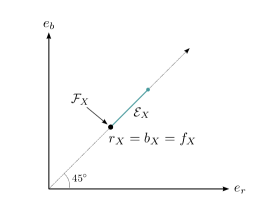
Figure 12. Depiction of the fairness-accuracy frontier under assumption of strong independence

O.6. Microfoundations for the FA frontier

We now provide a foundation of our FA frontier as the optimal points for different classes of FA preferences. First, consider the following utility over errors

$$w\left(e_{r},e_{b}\right)=\alpha_{r}e_{r}+\alpha_{b}e_{b}+\alpha_{f}\left|e_{r}-e_{b}\right|$$

where $\alpha_{r},\alpha_{b}<0$ and $\alpha_{f}\leq 0$. Call the corresponding preference of this utility simple. Simple preferences are FA preferences. For example, both the Utilitarian and Rawlsian preferences are simple. To see this for the Utilitarian designer, set $\alpha_{r}=-p_{r}$, $\alpha_{b}=-p_{b}$ and $\alpha_{f}=0$. To see this for the Rawlsian designer, set $\alpha_{r}=\alpha_{b}=\alpha_{f}=-1$.

Given any FA preference $\succeq$, let

$$\mathcal{F}_{X}(\succeq)=\left\{e\in\mathcal{E}_{X}\text{ : }e\succeq e^{\prime}\text{ for all }e^{\prime}\in\mathcal{E}_{X}\right\}$$

denote the set of $\succeq$-optimal points. We now provide the following characterizations of the FA frontier.

Proposition O.5.

The following are equivalent:

1. $e\in\mathcal{F}_{X}$

2. $e\in\mathcal{F}_{X}(\succeq)$ for some FA preference $\succeq$

3. $\left\{e\right\}=\mathcal{F}_{X}(\succeq)$ for some FA preference $\succeq$

4. $e\in\mathcal{F}_{X}(\succeq)$ for some simple FA preference $\succeq$

The above result shows that our FA frontier is the set of all optimal points for all FA preferences. Moreover, $\mathcal{F}_{X}$ is minimal in the sense that we cannot exclude any points from $\mathcal{F}_{X}$ without hurting some designer. This is because for every point $e\in\mathcal{F}_{X}$, there exists some FA preference $\succeq$ such that $e$ is the unique optimal error pair given $\succeq$ within the feasible set $\mathcal{E}_{X}$. Finally, our FA frontier also corresponds to the optimal points for all simple FA preferences.

Proof.

We will first show that (3) implies (2) implies (1) implies (3). Note that (3) implies (2) is trivial. To see why (2) implies (1), suppose $e\in\mathcal{F}_{X}(\succeq)$ for some FA preference $\succeq$ but $e\not\in\mathcal{F}_{X}$. Thus, there exists some $e^{\prime}>_{FA}e$ so $e^{\prime}\succ e$ yielding a contradiction.

We now prove that (1) implies (3). Fix some $e^{*}\in\mathcal{F}_{X}$ and let $h:\mathbb{R}\rightarrow\left(0,1\right)$ be a strictly decreasing function. Define

$$w\left(e\right)=\begin{cases}1+h\left(e_{r}+e_{b}\right)&\text{if }e=e^{\ast}\text{ or }e>_{FA}e^{\ast}\\ h\left(e_{r}+e_{b}\right)&\text{otherwise}\end{cases}$$

and let $\succeq$ be the corresponding preference. We will show that $\succeq$ is an FA preference. Suppose $e>_{FA}e^{\prime}$ so $h\left(e_{r}+e_{b}\right)>h\left(e_{r}^{\prime}+e_{b}^{\prime}\right)$. If both points FA-dominate $e^{\ast}$ or neither do, then $w\left(e\right)>w\left(e^{\prime}\right)$. The only remaining case is when $e>_{FA}e^{\ast}$ but $e^{\prime}$ does not FA-dominate $e^{\ast}$, in which case

$$w\left(e\right)=1+h\left(e_{r}+e_{b}\right)>1>h\left(e_{r}^{\prime}+e_{b}^{\prime}\right)=w\left(e^{\prime}\right)$$

Thus, $\succeq$ is an FA preference. Now, since $e^{*}\in\mathcal{F}_{X}$, there exists no other $e\in\mathcal{E}_{X}$ such that $e>_{FA}e^{\ast}$. That means that for all $e\in\mathcal{E}_{X}\backslash\left\{e^{\ast}\right\}$, $w\left(e^{\ast}\right)>w\left(e\right)$ so $\left\{e^{\ast}\right\}=\mathcal{F}_{X}(\succeq)$. This proves (3).

Finally, we show the equivalence of (1) and (4). Note that (4) implies (2) which implies (1) from above. We now show that (1) implies (4). Fix some $e^{*}\in\mathcal{F}_{X}$, so by Theorem 3.1, $e^{*}$ must either belong to the lower boundary from $r_{X}$ to $b_{X}$ or the lower boundary from $b_{X}$ to $f_{X}$, where the latter case only happens when $X$ is $r$-skewed (we omit the symmetric situation when $X$ is $b$-skewed). If $e^{*}$ belongs to the boundary from $r_{X}$ to $b_{X}$, then from the proof of Theorem 3.1 we know that $e^{*}$ belongs to an edge of this boundary that has negative slope. Thus there exists a vector $(\alpha_{r},\alpha_{b})$ that is normal to this edge, such that $e^{*}$ maximizes $\alpha_{r}e_{r}+\alpha_{b}e_{b}$ among all feasible points. Since this edge has negative slope, it is straightforward to see that $\alpha_{r},\alpha_{b}<0$. So $e$ maximizes the simple utility $\alpha_{r}e_{r}+\alpha_{b}e_{b}$ as desired.

If instead $X$ is $r$-skewed and $e^{*}$ belongs to the boundary from $b_{X}$ to $f_{X}$, then again $e^{*}$ belongs to an edge of this boundary. But now this edge must have weakly positive slope (since the edge starting from $b_{X}$ has weakly positive slope by the definition of $b_{X}$, and since the boundary is convex). In addition, this slope must be strictly smaller than $1$ because otherwise $f_{X}$ would be farther away from the 45-degree line compared to its adjacent vertex on this boundary. It follows that the outward normal vector $(\beta_{r},\beta_{b})$ to the edge that $e^{*}$ belongs to satisfies $\beta_{r}\geq 0\geq-\beta_{r}>\beta_{b}$. The point $e^{*}$ of interest maximizes $\beta_{r}e_{r}+\beta_{b}e_{b}$ among all feasible points. Now let us choose any $\alpha_{f}$ to belong to the interval $(\beta_{b},-\beta_{r})$, which is in particular negative. Further define $\alpha_{r}=\beta_{r}+\alpha_{f}<0$ and $\alpha_{b}=\beta_{b}-\alpha_{f}<0$. Then $\beta_{r}e_{r}+\beta_{b}e_{b}$ can be rewritten as $\alpha_{r}e_{r}+\alpha_{b}e_{b}+\alpha_{f}(e_{b}-e_{r})$. If we consider the simple utility $\alpha_{r}e_{r}+\alpha_{b}e_{b}+\alpha_{f}|e_{b}-e_{r}|$, then for any other feasible point $e^{**}$ it holds that

$$\alpha_{r}e_{r}^{**}+\alpha_{b}e_{b}^{**}+\alpha_{f}|e_{b}^{**}-e_{r}^{**}| \leq\alpha_{r}e_{r}^{**}+\alpha_{b}e_{b}^{**}+\alpha_{f}(e_{b}^{**}-e_{r}^{**})$$

$$=\beta_{r}e_{r}^{**}+\beta_{b}e_{b}^{**}$$

$$\leq\beta_{r}e_{r}^{*}+\beta_{b}e_{b}^{*}$$

$$=\alpha_{r}e_{r}^{*}+\alpha_{b}e_{b}^{*}+\alpha_{f}(e_{b}^{*}-e_{r}^{*})$$

$$=\alpha_{r}e_{r}^{*}+\alpha_{b}e_{b}^{*}+\alpha_{f}|e_{b}^{*}-e_{r}^{*}|,$$

where the first inequality holds since $\alpha_{f}\leq 0$ and the last equality holds because $e^{*}\in\mathcal{F}_{X}$ must be weakly above the 45-degree line. Hence the above inequality shows that $e^{*}$ maximizes the simple utility we have constructed, completing the proof. ∎

O.7. Fairness Criteria in the Literature

We review here certain fairness criteria that have appeared in the literature, and explain how these criteria can be accommodated within our framework.

O.7.1. Statistical Parity.

This criterion seeks equality in decisions, namely that the proportion of either group receiving the two decisions is the same (Dwork et al., 2012). Formally, an algorithm $a$ satisfies statistical parity if

$$\mathbb{E}(a(X)=1\mid G=r)-\mathbb{E}(a(X)=1\mid G=b)=0$$

The loss function

$$\ell(d,y)=\left\{\begin{array}[]{cc}1&\mbox{ if }d=1\\ 0&\mbox{ otherwise}\end{array}\right.$$

returns a relaxed version of this criterion, since

$$e_{g}(a)=\mathbb{E}\left[\ell(a(X),Y)\mid G=g\right]=\mathbb{E}\left[a(X)=1\mid G=g\right]$$

so $|e_{r}(a)-e_{b}(a)|$ is the absolute difference in the probability that a group-$r$ individual and a group-$b$ individual receive the decision $d=1$.

O.7.2. False Positives.

Another common fairness criterion is equality of false positives across two groups (Angwin and Larson, 2016; Chouldechova, 2017; Kleinberg et al., 2017). For example, among borrowers who would not have defaulted on their loan if approved, prediction of default should be equal across the two groups. Formally, an algorithm $a$ satisfies equality of false positive rates if

$$\mathbb{E}(a(X)=1,Y=0\mid G=r)-\mathbb{E}(a(X)=1,Y=0\mid G=b)=0$$

The loss function

$$\ell(d,y)=\left\{\begin{array}[]{cc}1&\mbox{ if }(d,y)=(1,0)\\ 0&\mbox{ otherwise}\end{array}\right.$$

returns a relaxed version of this criterion, since

$$e_{g}(a)=\mathbb{E}\left[\ell(a(X),Y)\mid G=g\right]=\mathbb{E}\left[a(X)=1,Y=0\mid G=g\right]$$

is the false-positive rate for group $g$, and so $|e_{r}(a)-e_{b}(a)|$ is the absolute difference in false positive rates. A fairness criterion based on the difference in false negative rates can be accommodated similarly.

O.7.3. Equalized Odds.

Another popular fairness criterion asks for equalized odds (Hardt et al., 2016), which an algorithm $a$ satisfies if

(O.4) $$\mathbb{E}_{Y}[\mathbb{E}_{X}[a(X)\mid G=r,Y]-\mathbb{E}_{X}[a(X)\mid G=b,Y]]=0$$

The inner difference compares the average decision for group-$r$ and group-$b$ individuals who share the same type $Y$, and the outer expectation averages over those values of $Y$.

The group-dependent loss function

$$\ell(d,y,g)=\left\{\begin{array}[]{cc}\frac{P(Y=y)}{P(Y=y\mid G=g)}&\mbox{ if }d=1\\ 0&\mbox{otherwise}\end{array}\right.$$

returns a relaxed version of this criterion, since

$$\mathbb{E}[\ell(d,y,g)\mid G=r] =P(Y=0\mid G=r)\times\mathbb{E}\left[\frac{P(Y=0)}{P(Y=0\mid G=r)}\times\mathbbm{1}(d=1)\mid G=r,Y=0\right]$$

$$\quad+P(Y=1\mid G=r)\times\mathbb{E}\left[\frac{P(Y=1)}{P(Y=1\mid G=r)}\times\mathbbm{1}(d=1)\mid G=r,Y=1\right]$$

$$=P(Y=0)\times\mathbb{E}[\mathbbm{1}(d=1)\mid G=r,Y=0]$$

$$\hskip 56.9055pt+P(Y=1)\times\mathbb{E}[\mathbbm{1}(d=1)\mid G=r,Y=1]$$

so $|\mathbb{E}[\ell(a(X),Y,G)\mid G=r]-\mathbb{E}[\ell(a(X),Y,G)\mid G=b]|$ is exactly the LHS of (O.4). As discussed in footnote 12, all of our results hold also for this group-dependent loss function.

References

- Agan and Starr (2018) Agan, A. and S. Starr (2018): “Ban the Box, Criminal Records, and Racial Discrimination: A Field Experiment,” The Quarterly Journal of Economics, 133, 191–235.
- Agarwal et al. (2018) Agarwal, A., A. Beygelzimer, M. Dudík, J. Langford, and H. Wallach (2018): “A Reductions Approach to Fair Classification,” in ICML.
- Alonso and Câmara (2016) Alonso, R. and O. Câmara (2016): “Persuading Voters,” American Economic Review, 106, 3590–3605.
- Andreoni and Miller (2002) Andreoni, J. and J. Miller (2002): “Giving According to GARP,” Econometrica, 70, 737–753.
- Angwin and Larson (2016) Angwin, J. and J. Larson (2016): “Machine bias,” ProPublica.
- Arnold et al. (2021) Arnold, D., W. Dobbie, and P. Hull (2021): “Measuring Racial Discrimination in Algorithms,” AEA Papers and Proceedings, 111, 49—54.
- Bergemann and Morris (2019) Bergemann, D. and S. Morris (2019): “Information Design: A Unified Perspective,” Journal of Economic Literature, 57, 44–95.
- Bertrand and Kamenica (2020) Bertrand, M. and E. Kamenica (2020): “Coming apart? Cultural distances in the United States over time,” Working Paper.
- Blattner et al. (2022) Blattner, L., S. Nelson, and J. Spiess (2022): “Unpacking the Black Box: Regulating Algorithmic Decisions,” Working Paper.
- Bolton and Ockenfels (2000) Bolton, G. E. and A. Ockenfels (2000): “ERC: A Theory of Equity, Reciprocity, and Competition,” American Economic Review, 90, 166–193.
- Caplin et al. (2023) Caplin, A., D. Martin, and P. Marx (2023): “Modeling Machine Learning,” Working Paper.
- Chan and Eyster (2003) Chan, J. and E. Eyster (2003): “Does Banning Affirmative Action Lower College Student Quality?” American Economic Review, 93, 858–872.
- Charness and Rabin (2002) Charness, G. and M. Rabin (2002): “Understanding Social Preferences with Simple Tests,” The Quarterly Journal of Economics, 117, 817–869.
- Che et al. (2019) Che, Y.-K., K. Kim, and W. Zhong (2019): “Statistical Discrimination in Ratings-Guided Markets,” Working Paper.
- Chohlas-Wood et al. (2021) Chohlas-Wood, A., M. Coots, E. Brunskill, and S. Goel (2021): “Learning to be Fair: A Consequentialist Approach to Equitable Decision-Making,” Working Paper.
- Chouldechova (2017) Chouldechova, A. (2017): “Fair Prediction with Disparate Impact: A Study of Bias in Recidivism Prediction Instruments.” Big Data, 5, 153–163.
- Corbett-Davis et al. (2017) Corbett-Davis, S., E. Pierson, A. Feller, S. Goel, and A. Huq (2017): “Algorithmic decision-making and the cost of fairness,” in Proceedings of the 23rd Conference on Knowledge Discovery and Data Mining.
- Cowgill and Stevenson (2020) Cowgill, B. and M. T. Stevenson (2020): “Algorithmic Social Engineering,” AEA Papers and Proceedings, 110, 96–100.
- Cowgill and Tucker (2020) Cowgill, B. and C. E. Tucker (2020): “Algorithmic Fairness and Economics,” Working Paper.
- Curello and Sinander (2022) Curello, G. and L. Sinander (2022): “The Comparative Statics of Persuasion,” Working Paper.
- Dessein et al. (2022) Dessein, W., A. Frankel, and N. Kartik (2022): “Test-Optional Admissions,” Working Paper.
- Diana et al. (2021) Diana, E., T. Dick, H. Elzayn, M. Kearns, A. Roth, Z. Schutzman, S. Sharifi-Malvajerdi, and J. Ziani (2021): “Algorithms and Learning for Fair Portfolio Design,” in Proceedings of the 22nd ACM Conference on Economics and Computation.
- Dworczak et al. (2021) Dworczak, P., S. Kominers, and M. Akbarpour (2021): “Redistribution Through Markets,” Econometrica, 89, 1665–1698.
- Dwork et al. (2012) Dwork, C., M. Hardt, T. Pitassi, O. Reingold, and R. Zemel (2012): “Fairness through awareness,” in Proceedings of the 3rd Innovations in Theoretical Computer Science Conference, 214–226.
- Dwork and Roth (2014) Dwork, C. and A. Roth (2014): “The Algorithmic Foundations of Differential Privacy,” Found. Trends Theor. Comput. Sci., 9, 211–407.
- Ellison and Pathak (2021) Ellison, G. and P. A. Pathak (2021): “The Efficiency of Race-Neutral Alternatives to Race-Based Affirmative Action: Evidence from Chicago’s Exam Schools,” American Economic Review, 111, 943–75.
- Fehr and Schmidt (1999) Fehr, E. and K. M. Schmidt (1999): “A Theory of Fairness, Competition, and Cooperation,” The Quarterly Journal of Economics, 114, 817–868.
- Feigenberg and Miller (2021) Feigenberg, B. and C. Miller (2021): “Would Eliminating Racial Disparities in Motor Vehicle Searches have Efficiency Costs?*,” The Quarterly Journal of Economics, 137, 49–113.
- Ferry et al. (2022) Ferry, J., U. Aïvodji, S. Gambs, M.-J. Huguet, and M. Siala (2022): “Improving Fairness Generalization Through a Sample-Robust Optimization Method,” Machine Learning.
- Fisman et al. (2007) Fisman, R., S. Kariv, and D. Markovits (2007): “Individual Preferences for Giving,” American Economic Review, 97, 1858–1876.
- Fuster et al. (2021) Fuster, A., P. Goldsmith-Pinkham, T. Ramadorai, and A. Walther (2021): “Predictably Unequal? The Effects of Machine Learning on Credit Markets,” Journal of Finance.
- Garfinkel et al. (2018) Garfinkel, S. L., J. M. Abowd, and S. Powazek (2018): “Issues Encountered Deploying Differential Privacy,” in Proceedings of the 2018 Workshop on Privacy in the Electronic Society, New York, NY, USA: Association for Computing Machinery, WPES’18, 133–137.
- Garg et al. (2021) Garg, N., H. Li, and F. Monachou (2021): “Standardized Tests and Affirmative Action: The Role of Bias and Variance,” in Proceedings of the 2021 ACM Conference on Fairness, Accountability, and Transparency, New York, NY, USA: Association for Computing Machinery, FAccT ’21, 261.
- Hansen et al. (2022) Hansen, V. P. B., A. T. Neerkaje, R. Sawhney, L. Flek, and A. Søgaard (2022): “The Impact of Differential Privacy on Group Disparity Mitigation,” ArXiv, abs/2203.02745.
- Hardt et al. (2016) Hardt, M., E. Price, and N. Srebro (2016): “Equality of Opportunity in Supervised Learning,” in Advances in Neural Information Processing Systems, 3315–3323.
- Harsanyi (1953) Harsanyi, J. (1953): “Cardinal Utility in Welfare Economics and in the Theory of Risk-Taking,” Journal of Political Economy, 61, 434–435.
- Harsanyi (1955) ——— (1955): “Cardinal Welfare, Individualistic Ethics, and Interpersonal Comparison of Utility: Comment,” Journal of Political Economy, 63, 309–321.
- Ichihashi (2019) Ichihashi, S. (2019): “Limiting Sender’s Information in Bayesian Persuasion,” Games of Economic Behavior, 117, 276–288.
- Ichihashi (2023) ——— (2023): “Privacy, Transparency, and Policing,” .
- Jung et al. (2020) Jung, C., S. Kannan, C. Lee, M. Pai, A. Roth, and R. Vohra (2020): “Fair Prediction with Endogenous Behavior,” .
- Kamenica (2019) Kamenica, E. (2019): “Bayesian Persuasion and Information Design,” Annual Review of Economics, 11, 249–272.
- Kamenica and Gentzkow (2011) Kamenica, E. and M. Gentzkow (2011): “Bayesian Persuasion,” American Economic Review, 101, 2590–2615.
- Kasy and Abebe (2021) Kasy, M. and R. Abebe (2021): “Fairness, Equality, and Power in Algorithmic Decision-Making,” in ACM Conference on Fairness, Accountability, and Transparency.
- Klare et al. (2012) Klare, B. F., M. J. Burge, J. C. Klontz, R. W. Vorder Bruegge, and A. K. Jain (2012): “Face Recognition Performance: Role of Demographic Information,” IEEE Transactions on Information Forensics and Security, 7, 1789–1801.
- Kleinberg et al. (2018) Kleinberg, J., J. Ludwig, S. Mullainathan, and A. Rambachan (2018): “Algorithmic Fairness,” AEA Papers and Proceedings, 108, 22–27.
- Kleinberg and Mullainathan (2019) Kleinberg, J. and S. Mullainathan (2019): “Simplicity Creates Inequity: Implications for Fairness, Steretotypes, and Interpretability,” Working Paper.
- Kleinberg et al. (2017) Kleinberg, J., S. Mullainathan, and M. Raghavan (2017): “Inherent Trade-Offs in the Fair Determination of Risk Scores,” in 8th Innovations in Theoretical Computer Science Conference (ITCS 2017), vol. 67, 43:1–43:23.
- Lipton et al. (2018) Lipton, Z. C., A. Chouldechova, and J. McAuley (2018): “Does mitigating ML’s impact disparity require treatment disparity,” in 32nd Conference on Neural Information Processing Systems.
- Little et al. (2022) Little, C. O., M. Weylandt, and G. I. Allen (2022): “To the Fairness Frontier and Beyond: Identifying, Quantifying, and Optimizing the Fairness-Accuracy Pareto Frontier,” ArXiv.
- Loewenstein et al. (1989) Loewenstein, G. F., L. Thompson, and M. H. Bazerman (1989): “Social utility and decision making in interpersonal contexts,” Journal of Personality and Social Psychology, 57, 426–441.
- Ludwig and Mullainathan (2021) Ludwig, J. and S. Mullainathan (2021): “Algorithmic Behavioral Science: Machine Learning as a Tool for Scientific Discovery,” Working Paper.
- Lundberg (1991) Lundberg, S. J. (1991): “The Enforcement of Equal Opportunity Laws Under Imperfect Information: Affirmative Action and Alternatives,” The Quarterly Journal of Economics, 106, 309–326.
- Manski (2022) Manski, C. F. (2022): “Patient-centered appraisal of race-free clinical risk assessment,” Health Economics, 31, 2109–2114.
- Manski et al. (2022) Manski, C. F., J. Mullahy, and A. Venkataramani (2022): “Using Measures of Race to Make Clinical Predictions: Decision Making, Patient Health, and Fairness,” .
- Mehrabi et al. (2022) Mehrabi, N., F. Morstatter, N. Saxena, K. Lerman, and A. Galstyan (2022): “A Survey on Bias and Fairness in Machine Learning,” ACM Computing Surveys, 54, 1–35.
- Menon and Williamson (2018) Menon, A. K. and R. C. Williamson (2018): “The cost of fairness in binary classification,” in Proceedings of the 1st Conference on Fairness, Accountability and Transparency, ed. by S. A. Friedler and C. Wilson, PMLR, vol. 81 of Proceedings of Machine Learning Research, 107–118.
- Obermeyer et al. (2019) Obermeyer, Z., B. Powers, C. Vogeli, and S. Mullainathan (2019): “Dissecting racial bias in an algorithm used to manage the health of populations,” Science, 366, 447–453.
- Persico (2002) Persico, N. (2002): “Racial Profiling, Fairness, and Effectiveness of Policing,” American Economic Review, 92, 1472–1479.
- Rabin (1993) Rabin, M. (1993): “Incorporating Fairness into Game Theory and Economics,” American Economic Review, 83, 1281–1302.
- Rambachan et al. (2021) Rambachan, A., J. Kleinberg, S. Mullainathan, and J. Ludwig (2021): “An Economic Approach to Regulating Algorithms,” Working Paper.
- Rawls (1971) Rawls, J. (1971): A Theory of Justice, Harvard University Press.
- Rose (2021) Rose, E. K. (2021): “Who Gets a Second Chance? Effectiveness and Equity in Supervision of Criminal Offenders,” The Quarterly Journal of Economics, 136, 1199–1253.
- Rothstein (2004) Rothstein, J. M. (2004): “College performance predictions and the SAT,” Journal of Econometrics, 121, 297–317, higher Education (Annals Issue).
- Saez and Stantcheva (2016) Saez, E. and S. Stantcheva (2016): “Generalized Social Marginal Welfare Weights for Optimal Tax Theory,” American Economic Review, 106, 24–45.
- Sagawa et al. (2020) Sagawa, S., P. W. Koh, T. B. Hashimoto, and P. Liang (2020): “Distributionally Robust Neural Networks,” in International Conference on Learning Representations.
- Sullivan (2022) Sullivan, C. (2022): “Eliciting Preferences over Life and Death: Experimental Evidence from Organ Transplantation,” Working Paper.
- Systemwide Academic Senate (2020) Systemwide Academic Senate (2020): Report of the UC Academic Council Standardized Testing Task Force (STTF), University of California, Oakland, CA.
- Viviano and Bradic (2023) Viviano, D. and J. Bradic (2023): “Fair Policy Targeting,” Journal of the American Statistical Association.
- Vyas et al. (2020) Vyas, D. A., L. G. Eisenstein, and D. S. Jones (2020): “Hidden in Plain Sight — Reconsidering the Use of Race Correction in Clinical Algorithms,” New England Journal of Medicine, 383, 874–882.
- Wei and Niethammer (2020) Wei, S. and M. Niethammer (2020): “The Fairness-Accuracy Pareto Front,” ArXiv.
- Yang and Dobbie (2020) Yang, C. S. and W. Dobbie (2020): “Equal Protection Under Algorithms: A New Statistical and Legal Framework,” Michigan Law Review, 119.