Magnetograph Saturation and the Open Flux Problem

Abstract

Extrapolations of line-of-sight photospheric field measurements predict radial interplanetary magnetic field (IMF) strengths that are factors of $\sim$2–4 too low. To address this “open flux problem,” we reanalyze the magnetograph measurements from different observatories, with particular focus on those made in the saturation-prone Fe I 525.0 nm line by the Mount Wilson Observatory (MWO) and the Wilcox Solar Observatory (WSO). The total dipole strengths, which determine the total open flux, generally show large variations among observatories, even when their total photospheric fluxes are in agreement. However, the MWO and WSO dipole strengths, as well as their total fluxes, agree remarkably well with each other, suggesting that the two data sets require the same scaling factor. As shown earlier by Ulrich et al., the saturation correction $\delta^{-1}$ derived by comparing MWO measurements in the 525.0 nm line with those in the nonsaturating Fe I 523.3 nm line depends sensitively on where along the irregularly shaped 523.3 nm line wings the exit slits are placed. If the slits are positioned so that the 523.3 and 525.0 nm signals originate from the same height, $\delta^{-1}\sim 4.5$ at disk center, falling to $\sim$2 near the limb. When this correction is applied to either the MWO or WSO maps, the derived open fluxes are consistent with the observed IMF magnitude. Other investigators obtained scaling factors only one-half as large because they sampled the 523.3 nm line farther out in the wings, where the shift between the right- and left-circularly polarized components is substantially smaller.

1 Introduction

When extrapolated into the heliosphere, solar magnetograph measurements underestimate the radial interplanetary magnetic field (IMF) strength by factors of two or more (see, e.g., Wang & Sheeley 1988, 1995; Riley et al. 2014, 2019; Jian et al. 2015; Linker et al. 2017; Wallace et al. 2019; Badman et al. 2021). Two possible reasons for this large discrepancy (called the “open flux problem” by Linker et al. 2017) are that the magnetographs may be greatly underestimating the amount of large-scale flux threading the photosphere, or that the total amount of open magnetic flux on the Sun is much greater than predicted by the extrapolation models.

The most widely used technique for extrapolating line-of-sight measurements of the photospheric field into the corona and heliosphere is the potential-field source-surface (PFSS) method (Schatten et al. 1969; Altschuler & Newkirk 1969). In this idealized model, the magnetic field satisfies the current-free condition $\nabla\times\mbox{\boldmath{$B$}}=0$ out to a spherical “source surface” at heliocentric distance $r=R_{\rm ss}$, where the tangential field components are set to zero. At the inner boundary $r=R_{\odot}$, $B_{r}$ is matched to the observed photospheric field, which is deprojected by assuming it to be radial at the depth (below the temperature minimum) where it is measured (see Wang & Sheeley 1992). Contrary to the prescription of Altschuler & Newkirk (1969), the line-of-sight components are not matched because the photospheric field is nonpotential; instead, $B_{r}$ is taken to be conserved across the narrow “boundary layer” where the field makes the transition from radial/nonpotential to nonradial/potential. This assumption may break down if the magnetograph aperture size is much less than a supergranular radius ($\sim$20^′′), since some of the photospheric flux may then escape sideways as it fans out with height; however, continuity can be restored through spatial averaging, which will not affect the large-scale field that is the concern of this paper.

The total open flux is given by integrating the unsigned radial field over the source surface:

$$\Phi_{\rm open}(t)=R_{\rm ss}^{2}\int|B_{r}(R_{\rm ss},L,\phi,t)|d\Omega,$$ (1)

where $t$ denotes time, $L$ heliographic latitude, $\phi$ Carrington longitude, and $\Omega$ solid angle. Since the open flux is distributed isotropically at 1 AU according to Ulysses magnetometer observations (Balogh et al. 1995; Smith & Balogh 2008), the radial field strength at Earth ($r=r_{\rm E}$) is related to $\Phi_{\rm open}$ by

$$B_{\rm E}(t)=\frac{\Phi_{\rm open}(t)}{4\pi r_{\rm E}^{2}}.$$ (2)

The isotropization of the flux, which occurs by $r\sim 10$–15 $R_{\odot}$ (see, e.g., Wang 1996; Zhao & Hoeksema 2010; Cohen 2015), is due to the heliospheric sheet currents, which are not included in the PFSS model.

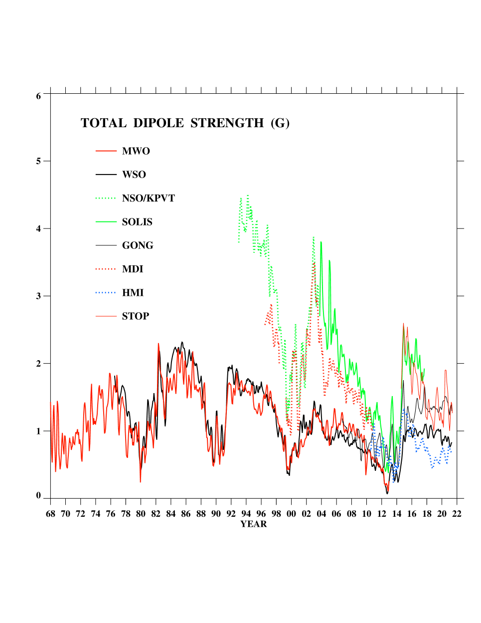
Figure 2: Comparison of the total dipole strengths $D_{\rm tot}$ derived from the photospheric field maps from MWO, WSO, KPVT/SPM, SOLIS, GONG, MDI, HMI, and STOP. The dipole component provides the main contribution to the source surface field and open flux, except during polar field reversal, when the quadrupole component dominates. Note that MWO and WSO show much weaker peaks in $D_{\rm tot}$ during 2002–2003 and 2014–2015 than the other observatories; these peaks also appear in the observed IMF variation (see Figure 1).

For the source surface radius $R_{\rm ss}$, the only free parameter in the PFSS model, a value of $2.5\pm 0.25$ $R_{\odot}$ has been shown to approximately reproduce the IMF sector structure during 1976–1982 (Hoeksema 1984) and the configuration of He I 1083.0 nm coronal holes during 1976–1995 (see Figure 2 in Wang et al. 1996). If such observational constraints are ignored, an obvious approach to reconciling the photospheric measurements with the observed radial IMF strength is simply to allow $R_{\rm ss}$ to take on much smaller values and to vary with time (see, e.g., Wang & Sheeley 1988; Lee et al. 2011; Linker et al. 2017; Bale et al. 2019; Badman et al. 2020). Virtanen et al. (2020) fitted the near-Earth IMF variation during 1967–2017 by varying $R_{\rm ss}$ between $\sim$3 and $\sim$1.5 $R_{\odot}$, and deduced that the solar corona abruptly shrank by more than a factor of two after the late 1990s. However, they provided no independent observational evidence to support this conclusion, other than the overall decline in sunspot activity since 2000. If the corona underwent such a contraction, the heliospheric current/plasma sheet extensions of helmet streamers would presumably also have moved inward, but SOHO/LASCO C2 images show little long-term change in the quasi-equilibrium positions of helmet streamer cusps, which continue to extend out to at least $r\sim 2.5$ $R_{\odot}$ as they did in 1996. Likewise, a long-term factor-of-two decrease in $R_{\rm ss}$ should be accompanied by a corresponding systematic increase in the areas of coronal holes, which (to our knowledge) has not been observed.

Comparisons between the PFSS model and extrapolations based on the magnetohydrodynamical (MHD) equations show generally good agreement in the predicted interplanetary sector structure and in the configuration of coronal holes (Neugebauer et al. 1998; Riley et al. 2006; Cohen 2015). The MHD models themselves depend on assumptions about the nature and global distribution of coronal heating, which effectively constitute a set of free parameters that replaces the source surface radius.

It has been suggested that the actual amount of open flux on the Sun may be much greater than that associated with visible coronal holes, either because the hole boundaries are not well defined or because small pockets of open flux are ubiquitous within closed regions. However, recent studies employing a wide variety of coronal hole detection techniques (Linker et al. 2021; Reiss et al. 2021) show that uncertainties in the locations of the hole boundaries cannot account for the large difference between the total open flux in coronal holes and the observed IMF strength; the discrepancy remains a factor of $\sim$2–4. Some of the disagreement in the inferred areal sizes of extreme-ultraviolet coronal holes could be due to the fanning-out of the hole boundaries with height, so that the line of sight traverses both the dark coronal hole and the brighter loop material underneath; since the amount of open flux is determined by the boundary at the photospheric level, the algorithms that predict the largest hole areas may be setting their intensity thresholds too high.

According to Fisk (2005), open flux is present outside coronal holes and is transported over the solar surface by undergoing interchange reconnection with closed loops. There has been no direct observational evidence for such a global random-walk process, which would require the complete breakdown of the current-free approximation in the quiet corona. The most likely site for continual interchange reconnection outside coronal holes is at their interface with the adjacent streamers; this may give rise to the raylike structure of the heliospheric plasma sheet that extends outward from the streamer cusps, but does not act to increase the total amount of open flux.

Riley et al. (2019) have speculated that most of the Sun’s polar flux may be hidden from view, but this seems unlikely (even allowing for instrumental noise) given that each pole is tilted toward Earth by 7^∘ once a year. The polar contribution to the open flux could be significantly underestimated if the field lines above latitude 70^∘ have a poleward tilt of $\sim$6^∘ at the photosphere, as suggested by Ulrich & Tran (2013). However, this effect would not be enough to double the open flux; nor would the many uncertainties associated with the construction of photospheric field maps, including the filling-in of missing polar data and the nonsimultaneous nature of the observations at different longitudes (see, e.g., Linker et al. 2017).

It has been proposed that the solar cycle variation of the near-Earth IMF strength is the result of interplanetary coronal mass ejections (see, e.g., Owens & Crooker 2006; Schwadron et al. 2010; Owens et al. 2011). However, ICMEs cannot account for the large post-maximum peaks in $B_{\rm E}$ observed during 1982, 1991, 2002–2003, and 2014–2015, which reflected increases in the Sun’s equatorial dipole strength associated with active longitudes or the emergence of large active-region complexes. In addition, using the ICME catalog of Richardson & Cane (2010), Wang & Sheeley (2015) showed that ICMEs contributed an average of only $\sim$20% to $B_{\rm E}$ during the maxima of cycles 23 and 24, consistent with the study of Richardson & Cane (2012). Riley (2007) derived a much larger contribution by setting the average radial field strength of an ICME to 8 nT, more than twice the observed value.

Recent measurements with the FIELDS instrument on the Parker Solar Probe show that $B_{r}r^{2}$ is approximately conserved from 1 to 0.13 au, so that the discrepancy between magnetograph extrapolations and the observed IMF strength persists very close to the Sun (Badman et al. 2021). This also suggests that the problem is not caused by the increasing prevalence of disconnected flux or magnetic switchbacks at greater heliocentric distances.

From this discussion, we are led to conclude that the solution to the open flux problem lies not in the extrapolation methods, in overlooked sources of open flux on the Sun, or in the topological properties of the IMF, but most likely in the magnetograph measurements themselves. This is hardly surprising, given the many uncertainties involved in interpreting these measurements, such as saturation effects when the Zeeman shift becomes comparable to the line width (e.g., Howard & Stenflo 1972; Frazier & Stenflo 1972; Ulrich 1992; Ulrich et al. 2009; Demidov & Balthasar 2009), weakening of the absorption lines due to the higher temperatures in magnetic regions (Chapman & Sheeley 1968; Harvey & Livingston 1969; Hirzberger & Wiehr 2005), the tendency for the magnetic flux to be concentrated in the dark intergranular lanes rather than the bright granular cell centers (Plowman & Berger 2020a,b,c), the fanning-out and weakening of the field with height, and the resulting dependence of the different effects on wavelength position relative to line center and on the center-to-limb angle, with horizontal field components or “fringing” becoming increasingly prevalent toward the limb.

In Section 2, we compare PFSS extrapolations of photospheric field maps from a variety ground- and space-based observatories/instruments, showing that the large differences in the predicted radial IMF strengths reflect differences in the measured dipole strengths, not in the photospheric fluxes. Section 3 focuses on the question of the saturation correction required for the Fe I 525.0 nm line used by the Mount Wilson Observatory (MWO) and the Wilcox Solar Observatory (WSO). The corrected MWO and WSO open fluxes are compared with the observed IMF variation in Section 4, where the contribution of ICMEs is also discussed. Our conclusions are summarized in Section 5.

2 Deriving the Open Flux Using Photospheric Field Maps from Different Observatories

As listed in Table 1, we employ synoptic maps of the photospheric magnetic field provided by MWO (1967–2013), WSO (1976–2021), National Solar Observatory (NSO) KPVT/SPM (1992–2003), SOHO/MDI (1996–2010), NSO/SOLIS/VSM (2003–2017), NSO/GONG (2006–2021), SDO/HMI (2010–2021), and Kislovodsk/STOP (2014–2021). No saturation corrections were applied to the data after downloading them from the observatory websites. In all cases, the photospheric field is assumed to be radially oriented and given by $B_{r}=B_{\rm los}/\cos{L}$, where the original line-of-sight measurements were taken around central meridian over a 27.3 day Carrington rotation (CR). The low-resolution MWO and WSO maps were interpolated to 5^∘ pixels in longitude and latitude, while the higher resolution maps from the other observatories were converted to a pixel size of 1^∘.

Both MWO and WSO employ the Fe I 525.0 nm line, which has a Landé factor $g=3.0$ and saturates at relatively low field strengths. The Ni I 676.8 nm line used by MDI and GONG is considerably less magnetically sensitive ($g=1.43$), while the lines adopted by KPVT (Fe I 868.8 nm; $g=1.67$), SOLIS and STOP (Fe I 630.15–630.25 nm; $g=1.67$/2.5), and HMI (Fe I 617.3 nm; $g=2.5$) have intermediate sensitivity.

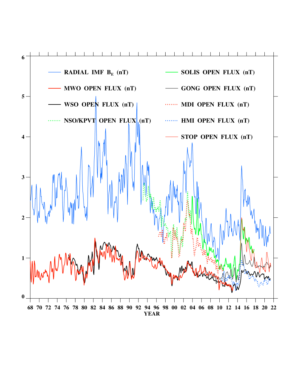
Figure 1: Comparison between the near-Earth radial IMF strength measured during 1968–2021 and the total open fluxes derived by applying a PFSS extrapolation to photospheric field maps from MWO, WSO, KPVT/SPM, SOLIS, GONG, MDI, HMI, and STOP. The source surface radius was fixed at $R_{\rm ss}=2.5$ $R_{\odot}$, $B_{r}$ was matched to the photospheric field on the assumption that it is radially oriented, and the total unsigned flux crossing the source surface was converted into a field strength at 1 au by dividing by $4\pi r_{\rm E}^{2}$. Daily values of $B_{x}$ measured near Earth were extracted from the OMNIWeb database and averaged without the sign over successive CRs. The MWO and WSO maps were interpolated to 72 longitude pixels by 36 latitude pixels, while the remaining maps were regridded to dimensions of 360$\times$180; no other corrections (other than for line-of-sight projection) were applied to the maps after downloading them from the observatory websites. Here and in the next three figures, all curves represent 3-CR running averages.

Figure 1 compares the observed radial IMF strength during 1968–2021 with the values predicted by applying a PFSS extrapolation to the photospheric field maps from the eight different observatories/instruments. For the near-Earth IMF measurements, we extracted daily values of $B_{x}$ from the OMNIWeb site and averaged them (without the sign) over each CR. To calculate the total open fluxes, the source surface radius was fixed at $R_{\rm ss}=2.5$ $R_{\odot}$ and $|B_{r}|$ was integrated over the source surface for each CR (Equation (1)); the results were then divided by $4\pi r_{\rm E}^{2}$ to convert them into field strengths at 1 au (Equation (2)). The plotted curves were smoothed by taking 3-CR running averages.

The values of $B_{\rm E}\propto\Phi_{\rm open}$ predicted by the observatories are spread over a wide range, sometimes differing by factors of up to $\sim$2–3, and they tend to be smaller than the measured IMF values by factors of $\sim$2–5. As an exception from the general trend, however, the KPVT/SPM open flux approximately matches the radial IMF measurements during 1992–1997, as found earlier by Arge et al. (2002). The SOLIS open flux also approaches the observed IMF levels during 2005–2009. The MWO and WSO open fluxes are in remarkably good agreement with each other, but both are a factor of $\sim$2 too low compared with the observed IMF near solar minimum and a factor of $\sim$4–5 too low near solar maximum.

Because the multipole components $l$ of the photospheric field fall off as $r^{-(l+2)}$, the main contribution to the source surface field and thus to $\Phi_{\rm open}$ comes from the dipole ($l=1$) component, except around the time of polar field reversal, when the quadrupole ($l=2$) dominates. The Sun’s total dipole strength, $D_{\rm tot}$, is given by

$$D_{\rm tot}(t)=(D_{\rm ax}^{2}+D_{\rm eq}^{2})^{1/2},$$ (3)

$$D_{\rm ax}(t)=\frac{3}{4\pi}\int B_{r}(R_{\odot},L,\phi,t)\sin{L}d\Omega,$$ (4)

$$D_{\rm eq}(t)=(H_{1}^{2}+H_{2}^{2})^{1/2},$$ (5)

$$H_{1}(t)=\frac{3}{4\pi}\int B_{r}(R_{\odot},L,\phi,t)\cos{L}\cos\phi d\Omega,$$ (6)

$$H_{2}(t)=\frac{3}{4\pi}\int B_{r}(R_{\odot},L,\phi,t)\cos{L}\sin\phi d\Omega.$$ (7)

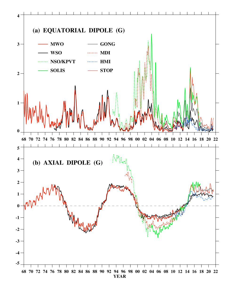
Figure 3: (a) Variation of $D_{\rm eq}$, the equatorial dipole or $(l=1,|m|=1)$ component of the photospheric field. (b) Variation of $D_{\rm ax}$, the axial dipole or $(l=1,m=0)$ component of the photospheric field. Although the amplitude of the axial dipole variation shows a wide scatter between observatories, the reversal times are in good agreement.

Figure 2 compares the values of $D_{\rm tot}$ derived for the different observatories, while Figure 3 shows separately the equatorial and axial components of the dipole vector. As anticipated, the variation of the total dipole strength resembles that of the total open flux for each observatory (compare Figures 1 and 2). The main difference is that the amplitude of the solar cycle variation is greater for $D_{\rm tot}$, which falls to very low values when $D_{\rm ax}$ reverses sign (see Figure 3(b)); at this time, $\Phi_{\rm open}$ is dominated by the quadrupole component of the photospheric field (CMEs also act to boost the observed IMF strength). From an analysis of white-light coronagraph data during 2012, Wang et al. (2014) deduced that the heliospheric current sheet split into two conical structures lying near the equator and separated by $\sim$180^∘ in longitude, consistent with the temporary prevalence of the $(l=2,|m|=2)$ harmonic component when $D_{\rm ax}$ goes through zero.

Comparing Figure 3(a) with Figure 1, we see that the large peaks in the IMF strength observed in 1982, 1991, 2002–2003, and 2014–2015 correspond to peaks in $D_{\rm eq}$. At these times, $|D_{\rm ax}|$ is also rapidly increasing and approaching its final solar-minimum level (Figure 3(b)); as a result, the post-maximum peaks in $D_{\rm tot}$, $\Phi_{\rm open}$, and the observed IMF strength are characterized by steep rises and more gradual falloffs. From Figures 1 and 2, we note that these peaks are much less prominent in the MWO and WSO extrapolations than in those using photospheric measurements from the other six observatories/instruments; this is especially clear during 2014–2015, when the WSO total open flux and dipole strength rise to a plateau but the SOLIS, GONG, HMI, and STOP extrapolations all predict a sharp peak, consistent with the IMF observations. The most likely reason for this difference is that the uncorrected MWO and WSO measurements overweight the fields toward the limb (or at higher latitudes), and thus $D_{\rm ax}$ relative to $D_{\rm eq}$ (see Section 4).

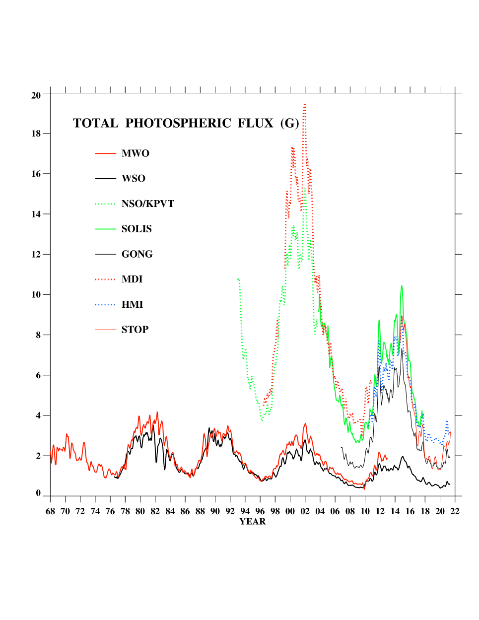
Figure 4: Variation of $B_{\rm tot}$, the total unsigned photospheric flux averaged over the solar surface. Agreement between total fluxes may (as in the case of MWO and WSO) or may not (as in the case of SOLIS and HMI) entail agreement between open fluxes or dipole strengths (compare Figure 4 with Figures 1 to 3).

Figure 4 shows, as a function of time for each of the observatories, the total unsigned photospheric flux, expressed as a surface-averaged field strength:

$$B_{\rm tot}(t)=\frac{1}{4\pi}\int|B_{r}(R_{\odot},L,\phi,t)|d\Omega.$$ (8)

In general, $B_{\rm tot}$ is dominated by high-order multipoles of the photospheric field, which fall off rapidly with height and do not contribute to $\Phi_{\rm open}$. Thus, agreement between the total fluxes measured by different observatories does not necessarily imply that their total dipole strengths or open fluxes agree, as may be seen by comparing Figure 4 with Figures 1 and 2. To better illustrate this point, Figure 5(a) shows the values of $B_{\rm tot}$ derived for HMI plotted against those derived for GONG, while Figure 5(b) shows the same for $D_{\rm tot}$. Here, each cross represents a CR. The HMI and GONG total photospheric fluxes display a tight linear relationship (with a slope of 1.04 and a correlation coefficient $cc=0.99$), but the relationship between their total dipole strengths is weak and noisy (with a slope of 0.14 and $cc=0.19$). Similarly, Figure 6 shows that the SOLIS total fluxes are on average a factor of 1.3 larger than the HMI total fluxes, but their dipole strengths are as much as a factor of 4.1 larger.

It is apparent that, when comparing magnetograph measurements in the context of the global solar field, pixel-by-pixel regression or histogram analyses of the photospheric flux itself, as in the study of Riley et al. (2014), do not properly capture the differences between the data sets. Instead, the focus should be on the differences between the lowest-order harmonic components, as in Virtanen & Mursula (2017) and in the present study.

3 The Correction Factor for the MWO and WSO Fields

For their long-term synoptic measurements, the MWO and WSO longitudinal magnetographs both employ the absorption line Fe I 525.0 nm, which has $g=3.0$. Since the line is also narrow, the Zeeman shift becomes comparable to the line width for even relatively weak fields. The shift is given by

$$\Delta\lambda_{\rm Z}=4.67\times 10^{-9}g\lambda^{2}B_{\rm los}\phantom{.}{\rm pm},$$ (9)

where $\lambda$ is in nanometers and $B_{\rm los}$ in gauss. The magnetograph signal may be represented by the Stokes parameter $V=(I_{+}-I_{-})/2$, where $I_{+}$ and $I_{-}$ denote the right- and left-circularly polarized intensities. For unsaturated fields,

$$V\simeq\Delta\lambda_{\rm Z}\frac{dI}{d\lambda}\propto gB_{\rm los}\frac{dI}{d\lambda}$$ (10)

(see, e.g., Stenflo 2013). In the case of Fe I 525.0 nm, however, the shifted line profile is no longer linear around the position of the exit slit, and Equation (10) breaks down.

Several different saturation corrections have been proposed, most of which involve comparing measurements made in Fe I 525.0 nm and Fe I 523.3 nm, which, because it is three times wider than the 525.0 nm line and has $g=1.3$, is assumed to remain unsaturated and to yield the true flux value. In addition, the 523.3 nm line is less prone to weakening due to the increased temperatures associated with the photospheric magnetic network (Chapman & Sheeley 1968; Harvey & Livingston 1969; Hirzberger & Wiehr 2005).

Using the MWO 150-foot tower telescope’s Babcock magnetograph and employing a 17${}^{\prime\prime}\times 17^{\prime\prime}$ scanning aperture, Howard & Stenflo (1972) made alternating measurements in the two lines and derived a scaling factor of

$$\delta^{-1}=\frac{B_{\rm los}(523.3)}{B_{\rm los}(525.0)}=0.48+1.33\cos\rho\qquad\textrm{(Howard \& Stenflo 1972)},$$ (11)

where $\rho$ is the center-to-limb angle (restricted to $\rho<60^{\circ}$). The magnetograph signal was interpreted as coming from a mixture of a “filamentary” component consisting of very narrow flux tubes with similar kilogauss field strengths and an “interfilamentary” component of less than 3 G; the measured flux densities reflect the varying filling factor of the filamentary component.

Frazier & Stenflo (1972) used the Kitt Peak multi-channel magnetograph to perform simultaneous observations in the two lines, with an aperture size of $2{\farcs}4\times 2{\farcs}4$. They obtained

$$\delta^{-1}=0.845+1.031\cos\rho\qquad\textrm{(Frazier \& Stenflo 1972)},$$ (12)

again giving a correction factor of 1.8–1.9 near disk center.

According to Svalgaard et al. (1978), the Stanford Solar Observatory (now WSO) used for its Fe I 525.0 nm measurements the same exit-slit arrangement as Howard & Stenflo (1972) at MWO. The most important difference between the instruments appears to be the 3^′ aperture size of the WSO magnetograph, which exceeds those employed at MWO by a factor of 10 or more. Svalgaard et al. made no comparison measurements in Fe I 523.3 nm or other lines, but instead assumed that the average field strength in a magnetic element is 1500 G and argued that the corresponding reading from their magnetograph would be 830 G; they thus obtained a saturation correction of 1.8 at disk center, in agreement with the result of Howard & Stenflo (1972) and Frazier & Stenflo (1972). In addition, by tracking magnetic flux as it rotated across the disk, they found that $B_{\rm los}(525.0)$ varied as $\cos\rho$; from this, they deduced that the saturation correction was independent of $\rho$ and that the center-to-limb variation of $B_{\rm los}(525.0)$ was that expected for the simple projection of a radially oriented photospheric field. They therefore concluded that

$$\delta^{-1}=1.8\qquad\textrm{(Svalgaard et al. 1978)}.$$ (13)

We remark here that, even though MWO magnetograms recorded in the 525.0 nm line do not show $B_{\rm los}$ falling off as $\cos\rho$ toward the limb, but instead remaining relatively strong, this does not necessarily require the photospheric field to be nonradial.

Employing the dual exit stage system of the post-1982 MWO magnetograph, Ulrich (1992) made simultaneous measurements in Fe I 525.0 nm and 523.3 nm with aperture sizes of $5^{\prime\prime}\times 5^{\prime\prime}$, $12^{\prime\prime}\times 12^{\prime\prime}$, and $20^{\prime\prime}\times 20^{\prime\prime}$. Rather surprisingly, the saturation correction was found to be more than twice as large as the values derived in the earlier studies: for the two larger apertures,

$$\delta^{-1}=4.5-2.5\sin^{2}\rho\qquad\textrm{(Ulrich 1992)},$$ (14)

with the $5^{\prime\prime}\times 5^{\prime\prime}$ aperture giving somewhat smaller values. As discussed below, Ulrich et al. (2009) later argued that this scaling factor should be reduced to

$$\delta^{-1}=4.15-2.82\sin^{2}\rho\qquad\textrm{(Ulrich et al. 2009)}.$$ (15)

Using the STOP magnetograph at the Syan Solar Observatory, Demidov & Balthasar (2009) obtained the full Stokes $I$ and $V$ profiles for both the 525.0 nm and 523.3 nm lines. They showed that the separation between the peaks of their Stokes $V$ profiles (normalized to the continuum intensity $I_{\rm c}$) is generally not a measure of the field strength. They also found that the Stokes $V/I_{\rm c}$ peak positions were close to the steepest parts of the corresponding Stokes $I$ profiles for both lines. To derive $B_{\rm los}(523.3)/B_{\rm los}(525.0)$, they took the ratio of the $V/I_{\rm c}$ peaks for the two lines, after averaging between the amplitudes of the blue- and red-wing peaks for each line and dividing out the respective Landé factors (see Equation (10)). The result for 10^′′ spatial resolution was

$$\delta^{-1}=1.74-2.43\cos\rho+3.43\cos^{2}\rho\qquad\textrm{(Demidov \& Balthasar 2009)},$$ (16)

with the disk center value of 2.74 increasing to 2.83 when the resolution was decreased to 100^′′.

As may be seen from Figures 1 through 4, the values of $\Phi_{\rm open}$, $D_{\rm tot}$, $D_{\rm eq}$, $D_{\rm ax}$, and $B_{\rm tot}$ derived from the MWO and WSO photospheric field maps are generally in excellent agreement with each other. This suggests that the MWO and WSO measurements require a similar correction factor (contrary to the conclusion of Riley et al. 2014), and that the constant scaling factor of 1.8 found by Svalgaard et al. (1978) using the WSO magnetograph cannot be correct if any of the $\rho$-dependent scaling factors derived at the other observatories are correct. One possible source of the disagreement is the much larger scanning aperture employed at WSO: it may be that the proportion of weak “interfilamentary” fields within the aperture increases systematically toward the limb, so that the $\cos\rho$ dependence of the measured line-of-sight field is partly coincidental.

Ulrich et al. (2009) presented a detailed analysis of the saturation corrections derived using the Fe I 523.3 nm line. Their main result was that the measured field depends sensitively on where in the 523.3 nm line wings the exit slits are placed. To demonstrate this, they used the MWO magnetograph (with a $12^{\prime\prime}\times 12^{\prime\prime}$ aperture) to scan the 523.3 nm line profile in both polarization states at a sampling interval of 0.53 pm, focusing their analysis on a sequence of profiles that they obtained for a plage region on 2007 July 13. Their Figure 6 shows how the Zeeman shift may be derived from the difference ($2\delta\lambda_{\rm bi}$) between the line bisector positions ($\lambda_{\rm bi}^{+}$, $\lambda_{\rm bi}^{-}$), defined for each state of polarization as being midway between a given pair of equal-intensity points on the red and blue wings of the line. The field strength is then obtained by setting $\Delta\lambda_{\rm Z}=\delta\lambda_{\rm bi}$ in Equation (9) above. However, the result depends sensitively on where along the 523.3 nm line profile the bisector is calculated, because the red and blue wings are asymmetric and their shapes also differ between the two polarization states.

The dependence of $B_{\rm los}(523.3)$ on $\Delta\lambda$, the position on the 523.3 nm line wing used to determine the bisector locations, is shown in Figure 7, where the curve is the same as that plotted in Figure 7 of Ulrich et al. (2009). We have superposed on this plot the center positions of the exit slits employed by Howard & Stenflo (1972), Frazier & Stenflo (1972), Ulrich (1992), Ulrich et al. (2009), and Demidov & Balthasar (2009). For the plage area under observation, $B_{\rm los}(523.3)$ ranges from a maximum value of $\sim$450 G at $\Delta\lambda\sim 8$ pm to a minimum value of $\sim$160 G at $\Delta\lambda\gtrsim 25$ pm. This sensitivity to where the 523.3 nm line profile is sampled may be one of the main reasons for the large differences among the 525.0 nm saturation corrections. In particular, Ulrich (1992) centered the 523.3 nm exit slit at $\Delta\lambda=8.7$ pm, near the peak of the curve in Figure 7, whereas Howard & Stenflo (1972) chose $\Delta\lambda=14$ pm; for the case shown in the figure, the derived values of $B_{\rm los}(523.3)$ would be $\sim$444 G and $\sim$275 G, respectively, representing a factor of $\sim$1.61 difference. Similarly, Frazier & Stenflo (1972) centered their 523.3 nm slit at $\Delta\lambda=16.2$ nm, which corresponds to $B_{\rm los}(523.3)\sim 227$ G according to Figure 7, a factor of $\sim$1.95 smaller than would be obtained with the slit positioned at 8.7 nm. Demidov & Balthasar (2009) used the bisector method to derive an estimate of the 525.0 nm saturation correction near disk center; in their illustrative case, they centered their “virtual” 523.3 nm slit at $\Delta\lambda=15.53$ pm and obtained $B_{\rm los}(523.3)/B_{\rm los}(525.0)\sim 2.46$.

Figure 7 raises the question of where exactly the 523.3 nm line profile should be sampled. Ulrich et al. (2009) suggested that the exit slit should be placed as close to the line center as possible, so that the field is measured at greater heights where it becomes more uniform. They chose $\Delta\lambda=2.9$ pm; because of the dip in the $B_{\rm los}(523.3)$ curve at small values of $\Delta\lambda$, the resulting saturation correction is then somewhat reduced relative to that derived by Ulrich (1992), who chose $\Delta\lambda=8.7$ pm (compare Equations (14) and (15)). However, the earlier (fortuitous) choice close to the peak of the curve may have been more appropriate, for the following reasons. Table 2 of Ulrich et al. (2009) gives the heights of formation of the 525.0 nm and 523.3 nm lines as a function of wavelength position and $\rho$, calculated using the Harvard–Smithsonian Reference Atmosphere and the radiative transfer methods described in Caccin et al. (1977), under the assumption of LTE. The radiation at the 525.0 nm slit position adopted by Ulrich (1992), $\Delta\lambda=3.9$ pm, comes from a height of $h=185$ km at disk center. For the 523.3 nm line (again for $\rho=0$), the estimated heights of formation corresponding to $\Delta\lambda=0.9$, 2.8, 8.4, 10.2, and 17.7 pm are $h=550$, 482, 145, 122, and 92 km, respectively. Thus, sampling the 523.3 nm line at $\Delta\lambda=2.9$ pm means that the signal originates from much greater heights than that recorded in the 525.0 nm line. Conversely, placing the slit at $\Delta\lambda=14$ pm (following Howard & Stenflo 1972) or 16.2 pm (following Frazier & Stenflo 1972) would cause the 523.3 nm signal to originate at substantially lower heights than the 525.0 nm signal. The original choice $\Delta\lambda=8.7$ pm makes the heights of formation of the 523.3 and 525.0 nm signals comparable to each other (see also Figure 4 in Ulrich et al. 2002).

A second reason for not placing the exit slit near the line center is that the photospheric field fans out with height on a horizontal scale comparable to a supergranule radius, or $\sim$20^′′ (the canopy effect). Since the scanning apertures used with the MWO magnetograph have dimensions $\lesssim 20^{\prime\prime}\times 20^{\prime\prime}$, some of the flux may escape sideways out of the aperture if the signal originates from heights of order 500 km, as is the case if $\Delta\lambda\lesssim 3$ pm. This might also be a reason for the decrease in $B_{\rm los}(523.3)$ near line center.

It is unclear to us why $B_{\rm los}(523.3)$ decreases steeply beyond $\Delta\lambda\sim 10$ pm, corresponding to heights below $\sim$120 km at disk center. Plowman & Berger (2020a,b,c) have suggested that unresolved granular structure at the photosphere causes magnetographs to underweight the strong flux in the dark intergranular lanes and to overweight the weak flux in the bright granule centers. However, G. J. D. Petrie (2021, private communication), using a different radiation MHD model for a sunspot and its surroundings, found almost no systematic correlation between intensity and field strength.

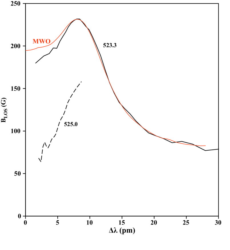
Figure 8: Field strengths $B_{\rm los}$ derived as a function of wavelength position $\Delta\lambda$ from NSO/FTS measurements of the Fe I 523.3 nm (solid black curve) and Fe I 525.0 nm (dashed black curve) line profiles. For comparison, the $B_{\rm los}(523.3)$ curve of Figure 7 has been scaled downward by a factor of $\sim$2 and replotted in red. The line bisector method was applied to FTS spectra in left- and right-circularly polarized light from a spotless plage region observed on 1979 April 30 at $\cos\rho=0.91$. Note the strong and opposite variations of $B_{\rm los}(525.0)$ and $B_{\rm los}(523.3)$ in the line wings, and the remarkable similarity between the shapes of the FTS and MWO $B_{\rm los}(523.3)$ curves, despite having been derived using completely different instruments and observing techniques. Ulrich (1992), Howard & Stenflo (1972), Frazier & Stenflo (1972), and Demidov & Balthasar (2009) centered their 525.0 nm exit slits at 3.9, 4.65, 5.5, and 6.21 pm, respectively. The much larger values of $\delta^{-1}$ obtained by Ulrich may be a consequence of adopting relatively small values of $\Delta\lambda$ for both his 523.3 and 525.0 nm measurements.

The shape of the $B_{\rm los}(523.3)$ versus $\Delta\lambda$ curve in Figure 7 has recently been confirmed by one of us (JWH) using Stokes $I$ and $V$ polarimetry data obtained with the McMath–Pierce/NSO Fourier Transform Spectrometer (FTS), as part of an ongoing survey of Zeeman splitting of a variety of spectral lines (J. W. Harvey, in preparation). On 1979 April 30, a spotless, unipolar region was observed at $\cos\rho=0.91$ using a 10^′′ circular aperture for a total integration time of 35 minutes. The wavelength range covered was $\sim$100 nm wide and centered at 505 nm, and included more than 2500 simultaneously recorded spectral lines. Line bisectors are here calculated for the 523.3 and 525.0 nm lines from their $I\pm V$ spectra. One-half the wavelength difference between the bisectors is scaled to $B_{\rm los}$ by Equation (9) and plotted in Figure 8 as a function of one-half the $I(\lambda)$ line width. Except for the different field strengths associated with the different plage regions under observation, the shapes of the 523.3 nm curves in Figures 7 and 8 are strikingly similar, despite the completely different instruments and observing techniques used to obtain them (to make this even clearer, the Figure 7 curve has been scaled down and replotted in red in Figure 8). Note that the $B_{\rm los}$ curves have opposite slopes for the two lines, increasing by a factor of more than two moving outward along the 525.0 nm wings, but decreasing by a factor of three in the wings of 523.3 nm beyond the peak at $\Delta\lambda\sim 8$ pm. This at least partly explains why the values of $\delta^{-1}$ found by different investigators are so discordant. Because Howard & Stenflo (1972), Frazier & Stenflo (1972), and Demidov & Balthasar (2009) placed their 525.0 nm exit slits somewhat farther away from line center than Ulrich (1992) (i.e., at 4.65, 5.5, and 6.21 pm rather than at 3.9 pm), the net result may have been to decrease further the $B_{\rm los}(523.3)/B_{\rm los}(525.0)$ ratios that they derived compared with that obtained by Ulrich (1992).

In addition to the line profile measurements that were the basis for their (and our) Figure 7, Ulrich et al. (2009) described a new set of MWO observations during 2007 April–May, in which they obtained pairs of magnetograms with the 525.0 nm slit position fixed at $\pm$3.9 pm (as in Ulrich 1992) and the 523.3 nm line sampled at $\pm$0.9, $\pm$2.9, $\pm$8.4, $\pm$10.2, and $\pm$17.7 pm. The scatter diagrams in their Figure 3 show the relationship between $B_{\rm los}(523.3)$ and $B_{\rm los}(525.0)$ for different $\rho$, for the case where the 523.3 nm slit is centered at $\pm$8.4 nm (near the peak of the curve in Figure 7). Near disk center ($0.0<\rho<0.4$), the regression line has a slope of $5.525\pm 0.107$, while near the limb ($0.8<\rho<0.95$) the slope is $2.757\pm 0.083$. The center-to-limb variation of $B_{\rm los}(523.3)/B_{\rm los}(525.0)$ may then be approximated as

$$\delta^{-1}=5.5-2.8\sin^{2}\rho.$$ (17)

This correction factor is even larger than that found by Ulrich (1992) employing an earlier MWO spectrograph system, and substantially exceeds the result obtained when the 523.3 nm slit is placed at $\pm$2.9 pm (Equation(15)).

4 Comparison with the Observed Radial IMF Variation

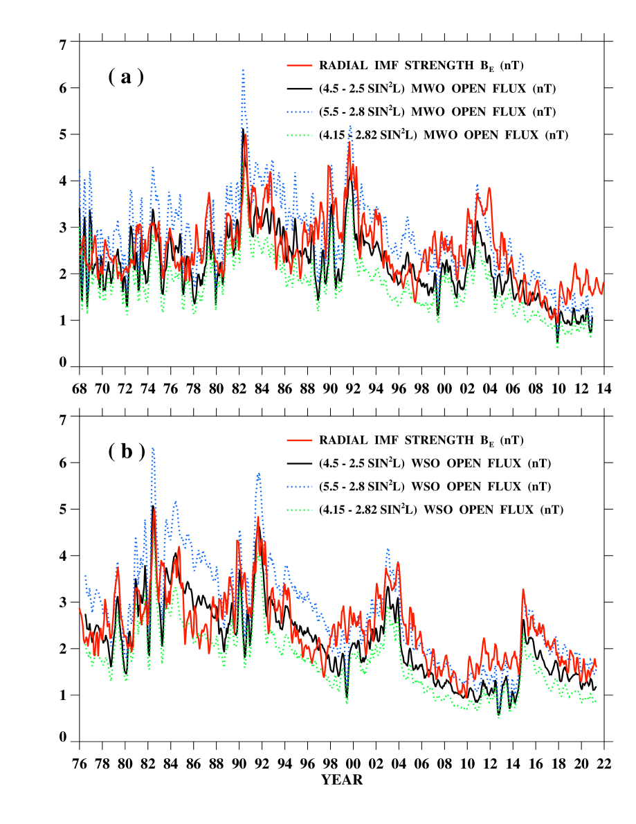
Figure 9: Comparison between the observed radial IMF strength during 1968–2021 and the total open fluxes derived from the (a) MWO and (b) WSO photospheric field maps, after applying three different versions of the Fe I 525.0 nm saturation correction: $\delta^{-1}=(4.5-2.5\sin^{2}L)$ (Ulrich 1992); $\delta^{-1}=(5.5-2.8\sin^{2}L)$ (Ulrich et al. 2009); and $\delta^{-1}=(4.15-2.82\sin^{2}L)$ (Ulrich et al. 2009). As in Figure 1, $R_{\rm ss}=2.5$ $R_{\odot}$ and all curves represent 3-CR running averages. The best overall fit is obtained using the $\delta^{-1}=(4.5-2.5\sin^{2}L)$ scaling factor.

We now apply the three Fe I 525.0 nm saturation corrections from Ulrich (1992) and Ulrich et al. (2009), given by Equations (14), (15), and (17), to the MWO and WSO photospheric field maps, and recalculate the total open fluxes using the PFSS model with $R_{\rm ss}=2.5$ $R_{\odot}$. The results are plotted in Figure 9, along with the near-Earth radial IMF variation during 1968–2021; all curves have been smoothed by taking 3-CR running means. The open fluxes obtained using the different corrections are all reasonably well correlated with the IMF variation, with $cc$ ranging from 0.71 to 0.76 when the MWO fields are extrapolated and from 0.79 to 0.86 when the WSO maps are employed. However, the values of $B_{\rm E}$ predicted with the $\delta^{-1}=(5.5-2.8\sin^{2}L)$ scaling factor (where we have replaced the center-to-limb angle $\rho$ by latitude $L$) are systematically too high before 1998, whereas the $\delta^{-1}=(4.15-2.82\sin^{2}L)$ scaling predicts values that are systematically too low (by an average of $\sim$29%) throughout the 53 yr interval. The best overall match to the observed IMF is obtained using the original $\delta^{-1}=(4.5-2.5\sin^{2}L)$ correction derived by Ulrich (1992). However, this scaling (like that for which $\delta^{-1}=4.15$ at $L=0$) gives values of $B_{\rm E}$ that are too low during the rising and maximum phases of the last two sunspot cycles.

It should be noted that all three correction factors give rise to prominent peaks in $\Phi_{\rm open}$ during 1982, 1991, 2002–2003, and 2014–2015, in agreement with the observed IMF variation. In contrast, the uncorrected values of the MWO and WSO open fluxes (Figure 1) and total dipole strengths (Figure 2) did not reproduce these peaks; they now appear because $\delta^{-1}(L)$ weights the low-latitude fields twice as much as the polar fields, increasing the strength of $D_{\rm eq}$ relative to $D_{\rm ax}$.

An inspection of Figure 9(b) also shows that, whichever saturation correction is adopted, the open fluxes derived from the WSO maps are systematically smaller relative to the observed IMF after $\sim$1998, as compared with earlier years (cf. Virtanen & Mursula 2017). This suggests that there may have been a decrease in the sensitivity of the WSO magnetograph sometime around 1998.

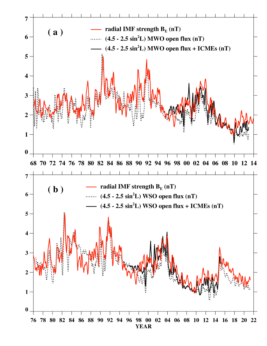
Figure 10: Effect of adding the contribution of ICMEs to the (a) MWO and (b) WSO total open fluxes, corrected using the $\delta^{-1}=(4.5-2.5\sin^{2}L)$ scaling factor. Near-Earth ICMEs during 1996–2015 were identified using the online Richardson–Cane catalog and assigned radial field strengths from the OMNIWeb database (see Wang & Sheeley 2015). ICMEs contributed $\sim$23% of the interplanetary flux during 1999–2002 and $\sim$18% during 2011–2014; their inclusion improves the agreement between the predicted and observed IMF strength during the rising and maximum phases of the solar cycle.

Wang & Sheeley (2015) estimated the contribution of ICMEs to the radial IMF strength at Earth during 1996–2015, including 457 events listed in the Richardson–Cane catalog and assigning to each ICME a radial field strength extracted from the OMNIWeb database. They found that, averaged over the interval 1999–2002 (2011–2014), ICMEs accounted for $\sim$23% ($\sim$18%) of the observed $B_{\rm E}$. Figure 10 shows the effect of adding the contribution of ICMEs to the MWO and WSO open fluxes, for the case where the saturation correction has the form $\delta^{-1}=(4.5-2.5\sin^{2}L)$. The observed IMF variation is sufficiently well reproduced as to suggest that this scaling factor and the inclusion of ICMEs provide a reasonable solution to the open flux problem.

5 Summary and Discussion

In addressing the open flux problem, we have focused on what we consider to be by far the “weakest link”: the magnetograph measurements themselves. Although Linker et al. (2017) and Riley et al. (2019) have argued that it is implausible that all of the different observatories should be systematically underestimating the photospheric flux, our analysis of the MWO and WSO measurements suggests that the uncertainties involved in interpreting the magnetograph signals are greater than sometimes supposed. We now summarize our conclusions.

1. When PFSS extrapolations with source surface at 2.5 $R_{\odot}$ are applied to (unmodified) photospheric field maps from MWO, WSO, KPVT, MDI, SOLIS, GONG, HMI, and STOP, the total open fluxes underestimate the observed radial IMF strength by factors of $\sim$2–5. An exception is the KPVT/SPM open flux, which briefly matched the IMF level during 1992–1997 (cf. Arge et al. 2002); the SOLIS values were also reasonably close to the observed level during 2005–2009.

2. Locating the source surface well inside $r\sim 1.5$ $R_{\odot}$ (see, e.g., Badman et al. 2020) would reduce the discrepancies, but would result in open field areas much larger than observed coronal holes and in closed field regions that do not extend outward as far as the LASCO C2 helmet streamers, whose cusps are located at and beyond $r\sim 2.5$ $R_{\odot}$.

3. The total open flux is determined by the lowest-order multipoles of the photospheric field, in particular the dipole and (during polar field reversal) quadrupole components. Because the total and local photospheric fluxes are dominated by high-order multipoles, agreement between the values of $B_{\rm tot}$ or $B_{\rm los}(R_{\odot},L,\phi)$ measured by different observatories does not imply that their dipole strengths or open fluxes agree. For example, the scatter plots in Figure 5 show that the HMI and GONG values of $B_{\rm tot}$ have a correlation of 0.99, with the regression line having a slope of 1.04, whereas their total dipole strengths $D_{\rm tot}$ have a correlation of 0.19 and a regression line slope of only 0.13. Similarly, the SOLIS values of $B_{\rm tot}$ are $\sim$1.3 times higher than the HMI values, but their total dipole strengths are as much as $\sim$4.1 times higher (Figure 6).

4. The values of $\Phi_{\rm open}$, $D_{\rm tot}$, and $B_{\rm tot}$ derived from the uncorrected MWO and WSO photospheric field maps are in remarkably good agreement with each other, indicating that they require approximately the same correction factor. Both observatories predict much weaker post-maximum peaks in $D_{\rm tot}$ and $\Phi_{\rm open}$ than the other observatories, suggesting that they underestimate the contribution of the equatorial dipole component, the main source of these peaks (which are also present in the observed IMF). A correction factor that is larger at low latitudes than near the poles would boost the relative strength of $D_{\rm eq}$ and make the MWO and WSO peaks more prominent.

5. The long-term synoptic measurements at MWO and WSO both employ the Fe I 525.0 nm absorption line, which has Landé factor $g=3.0$. Most of the correction factors that have been proposed are based on comparisons with measurements in the non-saturating Fe I 523.3 nm line ($g=1.3$). However, the values of $\delta^{-1}=B_{\rm los}(523.3)/B_{\rm los}(525.0)$ derived by Ulrich (1992) and Ulrich et al. (2009) are a factor of $\sim$2 higher than those found by Howard & Stenflo (1972), Frazier & Stenflo (1972), and Demidov & Balthasar (2009).

6. The constant factor of 1.8 correction obtained by Svalgaard et al. (1978) using the WSO magnetograph is the only one that is independent of center-to-limb angle $\rho$ and that is not based on comparisons with the 523.3 nm line (they simply assumed that the maximum signal of 830 G recorded with their instrument in the 525.0 nm line corresponded to an actual field strength of 1500 G). Their finding that $B_{\rm los}(525.0)\propto\cos\rho$ might be an artifact of the unusually wide (3^′) scanning aperture of the WSO instrument, if the larger and larger surface areas it averages over toward the limb include an increasing fraction of weak “interfilamentary” fields.

7. As shown by Ulrich et al. (2009), the field strength obtained using Fe I 523.3 nm depends sensitively on where along the line wing the exit slit is placed: $B_{\rm los}(523.3)$ peaks at $\Delta\lambda\sim 8$ pm but falls by a factor of $\sim$2 when $\Delta\lambda\sim 16$ pm. By centering the slit at $\Delta\lambda=8.7$ pm, Ulrich (1992) found that $\delta^{-1}=4.5$ at disk center, roughly twice the values obtained by Howard & Stenflo (1972), Frazier & Stenflo (1972), and Demidov & Balthasar (2009), who centered their slits at $\Delta\lambda=14$–16.2 pm.

8. We have argued that the 523.3 nm line profile should be sampled at the wavelength position whose associated height of origin is the same as that of the position where the 525.0 nm profile is sampled. Ulrich (1992) and Ulrich et al. (2009) placed their 525.0 nm exit slits at $\Delta\lambda=3.9$ pm. According to Table 2 of Ulrich et al. (2009), 525.0 nm $\pm$ 3.9 pm corresponds to a formation height $h=185$ km at disk center, reasonably close to the height of 145 km corresponding to 523.3 nm $\pm$ 8.4 pm. The radiation at 523.3 nm $\pm$ 14–16.2 pm (the slit positions adopted by Howard & Stenflo, Frazier & Stenflo, and Demidov & Balthasar) comes from lower in the atmosphere ($h\sim 100$ km).

9. Ulrich et al. (2009) suggested that the 523.3 nm profile should be sampled not at $\Delta\lambda\sim 8$ pm but closer to the line center, where the field becomes less structured and more uniform; they chose $\Delta\lambda=2.9$ pm, corresponding to a height of $\sim$480 km. Because $B_{\rm los}(523.3)$ falls to a local minimum at line center (Figure 7), the resulting correction factor $\delta^{-1}=(4.15-2.82\sin^{2}\rho)$ is somewhat smaller than that derived by Ulrich (1992) by taking $\Delta\lambda=8.7$ pm, $\delta^{-1}=(4.5-2.5\sin^{2}\rho)$. However, the formation height corresponding to the revised slit position is no longer consistent with the height of 185 km corresponding to the 525.0 nm slit position at $\Delta\lambda=3.9$ pm. Moreover, the total flux within the scanning aperture at $h\sim 480$ km may be less than that at the photospheric level because of the fanning-out of the field lines; indeed, this could be one reason for the dip in $B_{\rm los}(523.3)$ around line center. These arguments support the idea that the 523.3 nm line should be sampled near the peak of the curve in Figure 7, as was done by Ulrich (1992).

10. The shape of the $B_{\rm los}(523.3)$ curve in Figure 7 has been confirmed by one of us (JWH) by applying the line bisector method to spectropolarimetric data from NSO/FTS (Figure 8). The latter figure shows that $B_{\rm los}(525.0)$ is also a function of line profile position, but with the field strengths increasing rather than decreasing when moving outward along the wings.

11. Figure 9 shows that the best overall fit to the observed radial IMF variation during 1968–2021 is obtained by applying the $\delta^{-1}=(4.5-2.5\sin^{2}L)$ scaling factor to either the MWO or the WSO photospheric field maps. The fit is further improved by including ICMEs from the Richardson–Cane catalog, which contribute $\sim$20% of the IMF flux during the rising and maximum phases of the solar cycle (see Figure 10). We therefore suggest that the Ulrich (1992) saturation correction supplemented by ICMEs provides a plausible solution to the open flux problem.

An important question that remains to be answered is why the derived values of $B_{\rm los}(523.3)$ fall off steeply beyond $\Delta\lambda\sim 10$ pm, corresponding to heights $\lesssim$100 km. One possibility is that the circular polarization in the outer line wings is weakened through collisions, perhaps analogous to the collisional damping effect first discussed by Zanstra (1941) in the context of the depolarization of the Ca I 422.7 nm line wings near the solar limb. Such questions may serve as a reminder that the interpretation of the magnetograph signals from the variety of spectral lines listed in Table 1 is likely to be far from straighforward.

We are greatly indebted to L. Bertello, J. T. Hoeksema, Y. Liu, G. J. D. Petrie, A. A. Pevtsov, V. M. Pillet, N. R. Sheeley, Jr., L. Svalgaard, and A. G. Tlatov for helpful email discussions. The STOP maps were kindly made available to us by Dr. Tlatov. We have also utilized data from the NSO Integrated Synoptic Program, which is operated by the Association of Universities for Research in Astronomy under a cooperative agreement with NSF. This work was supported by NASA and the Office of Naval Research.

Table 1: Photospheric Magnetic Field Maps Used in This Study

Observatory/Instrument	Period Covered	Map Dimensions	Spectral Line	Landé $g$
Mount Wilson Observatory (MWO)	1967–2013 (CR 1516–2132)	91$\times$34	Fe I 525.0 nm	3.00
Wilcox Solar Observatory (WSO)	1976–present (CR 1642–present)	72$\times$30	Fe I 525.0 nm	3.00
NSO Kitt Peak Vacuum Telescope Spectromagnetograph (KPVT/SPM)	1992–2003 (CR 1863–2007)	360$\times$180	Fe I 868.8 nm	1.67
NSO SOLIS Vector Spectromagnetograph (SOLIS/VSM)	2003–2017 (CR 2007–2195)	360$\times$180	Fe I 630.15/630.25 nm	1.67/2.50
NSO Global Oscillation Network Group (GONG)	2006–present (CR 2047–present)	360$\times$180	Ni I 676.8 nm	1.43
Michelson Doppler Interferometer (MDI)	1996–1998, 1999–2010 (CR 1909–1937, 1947–2104)	3600$\times$1080	Ni I 676.8 nm	1.43
Helioseismic and Magnetic Imager (HMI)	2010–present (CR 2097–present)	720$\times$360	Fe I 617.3 nm	2.50
Kislovodsk Solar Telescope for Operative Predictions (STOP)	2014–present (CR 2152–present)	720$\times$360	Fe I 630.15/630.25 nm	1.67/2.50

Figure 5: Scatter plots of (a) $B_{\rm tot}$(HMI) against $B_{\rm tot}$(GONG), and (b) $D_{\rm tot}$(HMI) against $D_{\rm tot}$(GONG). Each cross represents a CR. Although the HMI and GONG total photospheric fluxes are in good agreement with each other (aside from a zero-point offset), their total dipole strengths are poorly correlated.

Figure 6: Scatter plots of (a) $B_{\rm tot}$(HMI) against $B_{\rm tot}$(SOLIS), and (b) $D_{\rm tot}$(HMI) against $D_{\rm tot}$(SOLIS). The SOLIS total fluxes are just 1.3 times larger than the HMI total fluxes, but their dipole strengths are 4.1 times larger than the corresponding HMI values.

Figure 7: Derived field strength $B_{\rm los}(523.3)$ as a function of $\Delta\lambda$, the wavelength position on the Fe I 523.3 nm line profile where the Zeeman shift is measured (using the line bisector method). The curve is reproduced from Figure 7 of Ulrich et al. (2009), and is based on left- and right-circularly polarized line profiles of a plage region observed with the MWO magnetograph on 2007 July 13. The vertical dotted lines mark the center positions of the exit slits used in the 523.3 nm measurements of Howard & Stenflo (1972), Frazier & Stenflo (1972), Ulrich (1992), Ulrich et al. (2009), and Demidov & Balthasar (2009). The curve peaks at $\Delta\lambda\sim 8$ pm, close to the slit position of Ulrich (1992). Howard & Stenflo, Frazier & Stenflo, and Demidov & Balthasar obtained lower values of $\delta^{-1}=B_{\rm los}(523.3)/B_{\rm los}(525.0)$ because they placed their slits farther out in the 523.3 nm line wings ($\Delta\lambda\sim 15$ pm), where $B_{\rm los}(523.3)$ falls by a factor of order 2. The slits had total widths of 16 pm (Howard & Stenflo 1972), 17.5 pm (Frazier & Stenflo 1972), 5.0 pm (Ulrich 1992; Ulrich et al. 2009), and 24.84 pm (Demidov & Balthasar 2009).

References

- (1)
- (2) Altschuler, M. D., & Newkirk, G., Jr. 1969, SoPh, 9, 131
- (3)
- (4) Arge, C. N., Hildner, E., Pizzo, V. J., & Harvey, J. W. 2002, JGR, 107, 1319
- (5)
- (6) Badman, S. T., Bale, S. D., Martínez Oliveros, J. C., et al. 2020, ApJS, 246, 23
- (7)
- (8) Badman, S. T., Bale, S. D., Rouillard, A. P., et al. 2021, A&A, 650, A18
- (9)
- (10) Bale, S. D., Badman, S. T., Bonnell, J. W., et al. 2019, Natur, 576, 237
- (11)
- (12) Balogh, A., Smith, E. J., Tsurutani, B. T., et al. 1995, Sci, 268, 1007
- (13)
- (14) Berezin, I. A., & Tlatov, A. G. 2020, Ge&Ae, 60, 872
- (15)
- (16) Brault, J. W. 1978, MmArc, 106, 33
- (17)
- (18) Caccin, B., Gomez, M. T., Marmolino, C., & Severino, G. 1977, A&A, 54, 227
- (19)
- (20) Chapman, G. A., & Sheeley, N. R., Jr. 1968, SoPh, 5, 442
- (21)
- (22) Cohen, O. 2015, SoPh, 290, 2245
- (23)
- (24) Demidov, M. L., & Balthasar, H. 2009, SoPh, 260, 261
- (25)
- (26) Fisk, L. A. 2005, ApJ, 626, 563
- (27)
- (28) Frazier, E. N., & Stenflo, J. O. 1972, SoPh, 27, 330
- (29)
- (30) Harvey, J., & Livingston, W. 1969, SoPh, 10, 283
- (31)
- (32) Hirzberger, J., & Wiehr, E. 2005, A&A, 438, 1059
- (33)
- (34) Hoeksema, J. T. 1984, PhD thesis, Stanford Univ.
- (35)
- (36) Howard, R., & Stenflo, J. O. 1972, SoPh, 22, 402
- (37)
- (38) Jian, L. K., MacNeice, P. J., Taktakishvili, A., et al. 2015, SpWea, 13, 316
- (39)
- (40) Lee, C. O., Luhmann, J. G., Hoeksema, J. T., et al. 2011, SoPh, 269, 367
- (41)
- (42) Linker, J. A., Caplan, R. M., Downs, C., et al. 2017, ApJ, 848, 70
- (43)
- (44) Linker, J. A., Heinemann, S. G., Temmer, M., et al. 2021, ApJ, 918, 21
- (45)
- (46) Liu, Y., Hoeksema, J. T., Scherrer, P. H., et al. 2012, SoPh, 279, 295
- (47)
- (48) Neugebauer, M., Forsyth, R. J., Galvin, A. B., et al. 1998, JGR, 103, 14587
- (49)
- (50) Norton, A. A., Pietarila Graham, J., Ulrich, R. K., et al. 2006, SoPh, 239, 69
- (51)
- (52) Owens, M. J., & Crooker, N. U. 2006, JGR, 111, A10104
- (53)
- (54) Owens, M. J., Crooker, N. U., & Lockwood, M. 2011, JGR, 116, A04111
- (55)
- (56) Pevtsov, A. A., Bertello, L., Nagovitsyn, Y. A., Tlatov, A. G., & Pipin, V. V. 2021, JSWSC, 11, 4
- (57)
- (58) Plowman, J. E., & Berger, T. E. 2020a, SoPh, 295, 142
- (59)
- (60) Plowman, J. E., & Berger, T. E. 2020b, SoPh, 295, 143
- (61)
- (62) Plowman, J. E., & Berger, T. E. 2020c, SoPh, 295, 144
- (63)
- (64) Reiss, M. A., Muglach, K., Möstl, C., et al. 2021, ApJ, 913, 28
- (65)
- (66) Richardson, I. G., & Cane, H. V. 2010, SoPh, 264, 189
- (67)
- (68) Richardson, I. G., & Cane, H. V. 2012, JSWSC, 2, A02
- (69)
- (70) Riley, P. 2007, ApJL, 667, L97
- (71)
- (72) Riley, P., Ben-Nun, M., Linker, J. A., et al. 2014, SoPh, 289, 769
- (73)
- (74) Riley, P., Linker, J. A., Mikić, Z., et al. 2006, ApJ, 653, 1510
- (75)
- (76) Riley, P., Linker, J. A., Mikic, Z., et al. 2019, ApJ, 884, 18
- (77)
- (78) Schatten, K. H., Wilcox, J. M., & Ness, N. F. 1969, SoPh, 6, 442
- (79)
- (80) Schwadron, N. A., Connick, D. E., & Smith, C. 2010, ApJL, 722, L132
- (81)
- (82) Smith, E. J., & Balogh, A. 2008, GeoRL, 35, L22103
- (83)
- (84) Stenflo, J. O. 2013, A&ARv, 21, 66
- (85)
- (86) Stenflo, J. O., Harvey, J. W., Brault, J. W., & Solanki, S. 1984, A&A, 131, 333
- (87)
- (88) Svalgaard, L., Duvall, T. L., Jr., & Scherrer, P. H. 1978, SoPh, 58, 225
- (89)
- (90) Tran, T., Bertello, L., Ulrich, R. K., & Evans, S. 2005, ApJS, 156, 295
- (91)
- (92) Ulrich, R. K. 1992, in ASP Conf. Ser. 26, Cool Stars, Stellar Systems, and the Sun, ed. M. S. Giampapa and J. A. Bookbinder (San Francisco, CA: ASP), 265
- (93)
- (94) Ulrich, R. K., Bertello, L., Boyden, J. E., & Webster, L. 2009, SoPh, 255, 53
- (95)
- (96) Ulrich, R. K., Evans, S., Boyden, J. E., & Webster, L. 2002, ApJS, 139, 259
- (97)
- (98) Ulrich, R. K., & Tran, T. 2013, ApJ, 768, 189
- (99)
- (100) Virtanen, I. I., Koskela, J. S., & Mursula, K. 2020, ApJL, 889, L28
- (101)
- (102) Virtanen, I., & Mursula, K. 2017, A&A, 604, A7
- (103)
- (104) Wallace, S., Arge, C. N., Pattichis, M., Hock-Mysliwiec, R. A., & Henney, C. J. 2019, SoPh, 294, 19
- (105)
- (106) Wang, Y.-M. 1996, ApJL, 456, L119
- (107)
- (108) Wang, Y.-M., Hawley, S. H., & Sheeley, N. R., Jr. 1996, Sci, 271, 464
- (109)
- (110) Wang, Y.-M., & Sheeley, N. R., Jr. 1988, JGR, 93, 11227
- (111)
- (112) Wang, Y.-M., & Sheeley, N. R., Jr. 1992, ApJ, 392, 310
- (113)
- (114) Wang, Y.-M., & Sheeley, N. R., Jr. 1995, ApJL, 447, L143
- (115)
- (116) Wang, Y.-M., & Sheeley, N. R., Jr. 2015, ApJL, 809, L24
- (117)
- (118) Wang, Y.-M., Young, P. R., & Muglach, K. 2014, ApJ, 780, 103
- (119)
- (120) Zanstra, H. 1941, MNRAS, 101, 273
- (121)
- (122) Zhao, X. P., & Hoeksema, J. T. 2010, SoPh, 266, 379
- (123)