The Kolmogorov Superposition Theorem can Break the Curse of Dimension When Approximating High Dimensional Functions

Abstract

We explain how to use Kolmogorov Superposition Theorem (KST) to break the curse of dimensionality when approximating a dense class of multivariate continuous functions. We first show that there is a class of functions called $K$-Lipschitz continuous in $C([0,1]^{d})$ which can be approximated by a special ReLU neural network of two hidden layers with a dimension independent approximation rate $O(n^{-1})$ with approximation constant increasing quadratically in $d$. The number of parameters used in such neural network approximation equals to $(6d+2)n$. Next we introduce KB-splines by using linear B-splines to replace the K-outer function and smooth the KB-splines to have the so-called LKB-splines as the basis for approximation. Our numerical evidence shows that the curse of dimensionality is broken in the following sense: When using the standard discrete least squares (DLS) method to approximate a continuous function, there exists a pivotal set of points in $[0,1]^{d}$ with size at most $O(nd)$ such that the rooted mean squares error (RMSE) from the DLS based on the pivotal set is similar to the RMSE of the DLS based on the original set with size $O(n^{d})$. In addition, by using matrix cross approximation technique, the number of LKB-splines used for approximation is the same as the size of the pivotal data set. Therefore, we do not need too many basis functions as well as too many function values to approximate a high dimensional continuous function $f$.

Key words: Kolmogorov Superposition Theorem, Functions Approximation, B-splines, Multivariate Splines Denoising, Sparse Solution, Pivotal Point Set

AMS Subject Classification: 41A15, 41A63, 15A23

1 Introduction

Recently, deep learning algorithms have shown a great success in many fronts of research, from image analysis, audio analysis, biological data analysis, to name a few. Incredibly, after a deep learning training of thousands of images, a computer can tell if a given image is a cat, or a dog, or neither of them with very reasonable accuracy. In addition, there are plenty of successful stories such that deep learning algorithms can sharpen, denoise, enhance an image after an intensive training. See, e.g. [22] and [46]. The 3D structure of a DNA can be predicted very accurately by using the DL approach. The main ingredient in DL algorithms is the neural network approximation based on ReLU functions. We refer to [10] and [12] for detailed explanation of the neural network approximation in deep learning algorithms.

Learning a multi-dimensional data set is like approximating a multivariate function. The computation of a good approximation suffers from the curse of dimension. For example, suppose that $f\in C([0,1]^{d})$ with $d\gg 1$. One usually uses Weierstrass theorem to have a polynomial $P_{f}$ of degree $n$ such that

$$\|f-P_{f}\|_{\infty}\leq\epsilon$$

for any given tolerance $\epsilon>0$. As the dimension of polynomial space $={n+d\choose n}\approx n^{d}$ when $n>d$, one will need at least $N=O(n^{d})$ data points in $[0,1]^{d}$ to distinguish different polynomials in $\mathbb{P}_{n}$ and hence, to determine this $P_{f}$. Notice that many good approximation schemes enable $P_{f}$ to approximate $f$ at the rate of $O((1/n)^{m})$ if $f$ is of $m$ times differentiable. In terms of the number $N$ of data points which should be greater than or equal to the dimension of polynomial space $\mathbb{P}_{n}$, i.e. $N\geq n^{d}$, the order of approximation is $O(1/(N^{1/d})^{m})$. When $d\gg 1$ is bigger, the order of approximation is less. This phenomenon is the so-called curse of dimension. Sometimes, such a computation is also called intractable. Similarly, if one uses a tensor product of B-spline functions to approximate $f\in C([0,1]^{d})$, one needs to subdivide the $[0,1]^{d}$ into $n^{d}$ small subcubes by hyperplanes parallel to the axis planes. As over each small subcube, the spline approximation $S_{f}$ of $f$ is a polynomial of degree $k$, e.g., $k=3$ if the tensor product of cubic splines are used. Even with the smoothness, one needs $N=O(k^{d})$ data points and function values at these data points in order to determine a polynomial piece of $S_{f}$ over each subcube. Hence, over all subcubes, one needs $O(n^{d}k^{d})$. It is known that the order of approximation of $S_{f}$ is $O(1/n^{k+1})$ if $f$ is of $k+1$ times coordinatewise differentiable. In terms of $N=O(n^{d}k^{d})$ points over $[0,1]^{d}$, the approximation order of $S_{f}$ will be $O(k^{k+1}/N^{(k+1)/d})$. More precisely, in [11], the researchers showed that the approximation order $O(1/N^{1/d})$ can not be improved for smooth functions in Sobolev space $W^{k,p}$ with $L_{p}$ norm $\leq 1$. In other words, the approximation problem by using multivariate polynomials or by tensor product B-splines is intractable.

Furthermore, many researchers have worked on using ridge functions, neural networks, and ReLU activation functions to approximate multidimensional functions. The orders of all these approximations in $L_{2}$ and in $L_{\infty}$ norms show the curse of dimensionality. See [45], [52], [53], [3] for detailed statements and proofs. That is, the approximation problem by using the neural networks is intractable. However, there is a way to obtain the dimension independent approximate rate as explained by Barron in [4]. Let $\Gamma_{B,C}$ be the class of functions $f$ defined over $B=\{{\bf x}\in\mathbb{R}^{d},\|{\bf x}\|\leq 1\}$ such that $C_{f}\leq C$, where $C_{f}$ is defined as follows:

$$C_{f}=\int_{\mathbb{R}^{d}}|\omega||\widetilde{f}(\omega)|d\omega$$

with $|\omega|=(\omega\cdot\omega)^{1/2}$ and $\widetilde{f}$ is the Fourier transform of $f$.

Theorem 1 (Barron, 1993)

For every function $f$ in $\Gamma_{B,C}$, every sigmoidal function $\phi$, every probability measure $\mu$, and every $n\geq 1$, there exists a linear combination of sigmoidal functions $f_{n}(x)$, a shallow neural network, such that

$$\int_{B}(f({\bf x})-f_{n}({\bf x}))^{2}d\mu({\bf x})\leq\frac{(2C)^{2}}{n}.$$

The coefficients of the linear combination in $f_{n}$ may be restricted to satisfy $\sum_{k=1}^{n}|c_{k}|\leq 2C$, and $c_{0}=f(0)$.

It is worthy of noting that although the approximation rate is independent of the dimension in the $L_{2}$ norm sense, the constant $C$ can be exponentially large in the worst case scenario as pointed out in [4]. This work leads to many recent studies on the properties and structures of Barron space $\Gamma_{B,C}$ and its extensions, e.g. the spectral Barron spaces and the generalization using ReLU or other more advanced activation functions instead of sigmodal functions above, e.g., [30], [14], [15], [16], [17], [57], [60], and the references therein. More recently, the super approximation power is introduced in [59] which uses the floor function, exponential function, step function, and their compositions as the activation function and can achieve the exponential approximation rate.

In this paper, we turn our attention to Kolmogorov superposition theorem (KST) and will see how it plays a role in the study of the rate of approximation for neural network computation in deep learning algorithms, how it can break the curse of dimension when approximating high dimensional functions over $\mathbb{R}^{d}$ for $d\geq 2$, and how we can realize the approximation so that it can overcome the curse of dimension when $d=2$ and $d=3$. For $d\geq 4$, see [58]. For convenience, we will use KST to stands for Kolmogorov superposition theorem for the rest of the paper. Let us start with the statement of KST using the version of G. G. Lorentz from [43] and [44].

Theorem 2 (Kolmogorov Superposition Theorem)

There exist irrational numbers $0<\lambda_{p}\leq 1$ for $p=1,\cdots,d$ and strictly increasing $Lip(\alpha)$ functions $\phi_{q}(x)$ (independent of $f$) with $\alpha=\log_{10}2$ defined on $I=[0,1]$ for $q=0,\cdots,2d$ such that for every continuous function $f$ defined on $[0,1]^{d}$, there exists a continuous function $g(u)$, $u\in[0,d]$ such that

$$f(x_{1},\cdots,x_{d})=\sum_{q=0}^{2d}g(\sum_{i=1}^{d}\lambda_{i}\phi_{q}(x_{i})).$$ (1)

Note that $\phi_{q},q=0,\cdots,2d$ are called K-inner functions or K-base functions while $g$ is called K-outer function. In the original version of KST (cf. [31] and [32]), there are $2d+1$ K-outer functions and $d(2d+1)$ inner functions. G. G. Lorentz simplified the construction to have one K-outer function and $2d+1$ inner functions with $d$ irrational numbers $\lambda_{i}$. It is known that $2d+1$ can not be smaller (cf. [13]) and the smoothness of the K-inner functions in the original version of the KST can be improved to be Lipschitz continuous (cf. [18]) while the continuity of $\phi_{q}$ in the Lorentz version can be improved to be $Lip_{\alpha}$ for any $\alpha\in(0,1)$ as pointed out in [44] at the end of the chapter. There were Sprecher’s constructive proofs (cf. [62, 63, 64, 65, 66, 67, 68, 69]) which were finally correctly established in [5] and [6]. An excellent explanation of the history on the KST can be found in [51] together with a constructive proof similar to the Lorentz construction.

Recently, KST has been extended to unbounded domain in [40] and has been actively studied during the development of the neural network computing (cf. e.g. [9], [47], [52], [49])) as well as during the fast growth period of the deep learning computation recently. Hecht-Nielsen [27] is among the first to explain how to use the KST as a feed forward neural network in 1987. In particular, Igelnik and Parikh [29] in 2003 proposed an algorithm of the neural network using spline functions to approximate both the inner functions and outer function $g$.

It is easy to see that the formulation of the KST is similar to the structure of a neural network where the K-inner and K-outer functions can be thought as two hidden layers when approximating a continuous function $f$. However, one of the main obstacles is that the K-outer function $g$ depends on $f$ and furthermore, $g$ can vary wildly even if $f$ is smooth as explained in [21]. Schmidt-Hieber [55] used a version of KST in [5] and approximated the K-inner functions by using a neural network of multiple layers to form a deep learning approach for approximating any Hölder continuous functions. Montanelli and Yang in [49] used very deep neural networks to approximate the K-inner and K-outer functions to obtain the approximation rate $O(n^{-\frac{1}{\log d}})$ for a function $f$ in the class $K_{C}([0,1]^{d})$ (see [49] for detail). That is, the curse of dimensionality is lessened. To the best of our knowledge, the approximation bounds in the existing work for general function still suffer the curse of dimensionality unless $f$ has a simple K-outer function $g$ as explained in this paper, and how to characterize the class of functions which has moderate K-outer functions remains an open problem. However, in the last section of this paper, we will provide a numerical method to test if a multi-dimensional continuous function is K-Lipschitz continuous.

The development of the neural networks obtains a great speed-up by using the ReLU function instead of a signmoidal activation function. Sonoda and Murata1 [61] showed that the ReLU is an approximator and established the universal approximation theorem, i.e. Theorem 3 below. Chen in [8] pointed out that the computation of layers in the deep learning algorithm based on ReLU is a linear spline and studied the upper bound on the number of knots needed for computation. Motivated by the work from [8], Hansson and Olsson in [26] continued the study and gave another justification for the two layers of deep learning are a combination of linear spline and used Tensorflow to train a deep learning machine for approximating the well-known Runge function using a few knots. There are several dissertations written on the study of the KST for the neural networks and data/image classification. See [7], [5], [19], [41], and etc..

The main contribution of this work is we propose to study the rate of approximation for ReLU neural network through KST. We propose a special neural network structure via the representation of KST, which can achieve a dimension independent approximation rate $O(n^{-1})$ with the approximation constant increasing quadratically in the dimension when approximating a dense subset of continuous functions. The number of parameters used in such a network increases linearly in $n$. Furthermore, we shall provide a numerical scheme to practically approximate $d$ dimensional continuous functions by using at most $O(dn)$ number of pivotal locations for function value evaluattion instead of the whole equally-spaced $O(n^{d})$ data locations, and such a set of pivotal locations are independent of target functions.

The subsequent sections of this paper are structured as follows. In section 2, we explain how to use KST to approximate multivariate continuous functions without the curse of dimensionality for a certain class of functions. We also establish the approximation result for any continuous function based on the modulus of continuity of the K-outer function. In section 3, we introduce KB-splines and its smoothed version LKB-splines. We will show that KB-splines are indeed the bases for functions in $C([0,1]^{d})$. In section 4, we numerically demonstrate in 2D and 3D that LKB-splines can approximate functions in $C([0,1]^{d})$ very well. Furthermore, we provide a computational strategy based on matrix cross approximation to find a sparse solution using a few number of LKB-splines to achieve the same approximation order as the original approximation. This leads to the new concept of pivotal point set from any dense point set $P$ over $[0,1]^{d}$ such that the discrete least squares (DLS) fitting based on the pivotal point set has the similar rooted mean squares error to the DLS fitting based on the original data set $P$.

2 ReLU Network Approximation via KST

We will use $\sigma_{1}$ to denote ReLU function through the rest of discussion. It is easy to see that one can use linear splines to approximate K-inner (continuous and monotone increasing) functions $\phi_{q},q=0,\cdots,2d$ and also approximate the K-outer (continuous) function $g$. We refer to Theorem 20.2 in [54]. On the other hand, we can easily see that any linear spline function can be written in terms of linear combination of ReLU functions and vice versa, see, e.g. [10], and [12]. (We shall include another proof later in this paper.) Hence, we have

$$L_{q}(t):=\sum_{j=1}^{N_{q}}c_{q,j}\sigma_{1}(t-y_{qj})\approx\phi_{q}(t)$$

for $q=0,\cdots,2d$ and

$$S_{g}(t):=\sum_{k=1}^{N_{g}}w_{k}\sigma_{1}(t-y_{k})\approx g,$$

where $g$ is the K-outer function of a continuous function $f$. Based on KST and the universal approximation theorem (cf. [9], [28], [52]), it follows that

Theorem 3 (Universal Approximation Theorem (cf. [61])

Suppose that $f\in C([0,1]^{d})$ is a continuous function. For any given $\epsilon>0$, there exist coefficients $w_{k},k=1,\cdots,N_{g}$, $y_{k}\in[0,d],k=1,\cdots,N_{g}$, $c_{q,j},j=1,\cdots,N_{i}$ and $y_{q,j}\in[0,1],j=1,\cdots,N_{i}$ such that

$$|f(x_{1},\cdots,x_{d})-\sum_{q=0}^{2d}\sum_{k=1}^{N_{g}}w_{k}\sigma_{1}(\sum_{i=1}^{d}\lambda_{i}\sum_{j=1}^{N_{q}}c_{q,j}\sigma_{1}(x_{i}-y_{qj})-y_{k})|\leq\epsilon.$$ (2)

In fact, many results similar to the above (2) have been established using other activation functions (cf. e.g. [9], [33], [49], and etc.).

2.1 K-Lipschitz Function

To establish the rate of convergence for Theorem 3, we introduce a new concept. For each continuous function $f\in C([0,1]^{d})$, let $g_{f}$ be the K-outer function associated with $f$. Let

$$KL=\{f:\hbox{ K-outer function $g_{f}$ is Lipschitz continuous}\}$$ (3)

be the class of K-Lipschitz continuous functions. Note that when $f$ is a constant, its K-outer function $g=\frac{1}{d+1}f$ is also constant (cf. [7]) and hence, is Lipschitz continuous. That is, the function class KL is not empty. On the other hand, we can use any univariate Lipschitz continuous function $g$ such as $g(t)=Ct,g(t)=\sin(Ct),g(t)=\exp(-Ct)$, $g(t)=\sin(Ct^{2}/2)$, etc.. over $[0,d]$ to define a multivariate function $f$ by using the formula (1) of KST, where $C$ is any constant. Then these newly defined $f$ are continuous over $[0,1]^{d}$ and are belong to the function class KL. It is easy to see that the class KL is dense in $C([0,1]^{d})$ by Weierstrass approximation theorem. See Lemma 4 below. For another example, let $g(t)$ be a B-spline function of degree $k\geq 1$, the associated multivariate function is in KL. We shall use such B-spline functions for the K-outer function $g$ approximation in a later section.

Theorem 4

For any $f\in C([0,1]^{d})$ and any $\epsilon>0$, there exists a K-Lipschitz continuous function $K$ such that

$$\|f-K\|_{\infty}\leq\epsilon.$$ (4)

• Proof. By Kolmogorov superposition theorem, we can write $f(x_{1},\cdots,x_{d})=\sum_{q=0}^{2d+1}g(\sum_{i=1}^{d}\lambda_{i}\phi_{q}(x_{i}))$. By Weierstrass approximation theorem, there exists a polynomial $p$ such that $|p(t)-g(t)|\leq\frac{\epsilon}{2d+1}$ for all $t\in[0,d]$. Such a polynomial $p$ is certainly a Lipschitz continuous function over $[0,d].$

  Therefore, by Letting $K(x_{1},\cdots,x_{d})=\sum_{q=0}^{2d+1}p(\sum_{i=1}^{d}\lambda_{i}\phi_{q}(x_{i}))\in KL$, we have

  $$|f(x_{1},\cdots,x_{d})-K(x_{1},\cdots,x_{d})| =|\sum_{q=0}^{2d+1}g(\sum_{i=1}^{d}\lambda_{i}\phi_{q}(x_{i}))-\sum_{q=0}^{2d+1}p(\sum_{i=1}^{d}\lambda_{i}\phi_{q}(x_{i}))|$$

  $$\leq\sum_{q=0}^{2d+1}|g(\sum_{i=1}^{d}\lambda_{i}\phi_{q}(x_{i}))-p(\sum_{i=1}^{d}\lambda_{i}\phi_{q}(x_{i}))|$$

  $$\leq(2d+1)\cdot\frac{\epsilon}{(2d+1)}=\epsilon.$$

  $\Box$

Note that the neural network being used for approximation in equation (2) is a special class of neural network with two hidden layers of widths $(2d+1)dN_{q}$ and $(2d+1)N_{g}$ respectively. Let us call this special class of neural networks the Kolmogorov network, or K-network in short and use $\mathcal{K}_{m,n}$ to denote the K-network of two hidden layers with widths $(2d+1)dm$ and $(2d+1)n$ based on ReLU activation function, i.e.,

$$\mathcal{K}_{m,n}(\sigma_{1})=\{\sum_{q=0}^{2d}\sum_{k=1}^{dn}w_{k}\sigma_{1}(\sum_{i=1}^{d}\sum_{j=1}^{m}c_{qj}\sigma_{1}(x_{i}-y_{qj})-y_{k}),w_{k},c_{qj}\in\mathbb{R},y_{k}\in[0,d],y_{qj}\in[0,1]\}.$$ (5)

The parameters in $\mathcal{K}_{m,n}$ are $w_{k},y_{k}$, $k=1,\cdots,dn$, and $c_{qj},y_{qj}$, $q=0,\cdots,2d$, $j=1,\cdots,m$. Therefore the total number of parameters equals to $2dn+2(2d+1)m$. In particular if $m=n$, the total number of parameters in this network is $(6d+2)n$. We are now ready to state one of the main results in this paper.

Theorem 5

Let $f\in C([0,1]^{d})$. Suppose that $f$ is in the KL class. Let $C_{f}$ be the Lipschitz constant of the K-outer function associated with $f$. We have

$$\inf_{s\in\mathcal{K}_{n,n}(\sigma_{1})}\|f-s\|_{C([0,1]^{d})}\leq\frac{C_{f}(2d+1)^{2}}{n}.$$ (6)

The significance of this result is, for a dense subclass of continuous functions, we need only $(6d+2)n$ parameters to achieve the approximation rate $O(n^{-1})$ with the approximation constant increasing quadratically in the dimension. That is, the curse of dimensionality is overcome for functions in this dense subclass. In other words, the computation becomes tractable. The above result improved the similar one in [49]. Also, the researchers in [50] showed that the KST can break the curse of dimension for band-limited functions. Our result breaks the curse of dimensionality for a different class of functions. On the other hand, many researchers used the smoothness of $f$ to characterize the approximation of ReLU neural networks. See [72], [42] and [73], where the approximation rate on the right-hand side of (6) is $O(n^{-s/d})$ with $s$ being the smoothness of the function $f$. Their approximation rates suffer from the curse of dimension. In terms of the smoothness of the K-outer function, our result above is believed to be the correct rate of convergence. In addition, we shall extend the argument to the setting of K-Hölder continuous functions and present the convergence in terms of K-modulus of smoothness.

2.2 Proof of Theorem 5

To prove Theorem 5, we need some preparations. Let us begin with the space $\mathcal{N}(\sigma_{1})=\hbox{span}\{\sigma_{1}({\bf w}^{\top}{\bf x}-b),b\in\mathbb{R},{\bf w}\in\mathbb{R}^{d}\}$ which is the space of shallow networks of ReLU functions. It is easy to see that all linear polynomials over $\mathbb{R}^{d}$ are in $\mathcal{N}(\sigma_{1})$. The following result is known (cf. e.g. [10]). For self-containedness, we include a different proof.

Lemma 1

For any linear polynomial $s$ over $\mathbb{R}^{d}$, there exist coefficients $c_{i}\in\mathbb{R}$, bias $t_{i}\in\mathbb{R}$ and weights ${\bf w}_{i}\in\mathbb{R}^{d}$ such that

$$s({\bf x})=\sum_{i=1}^{n}c_{i}\sigma_{1}({\bf w}_{i}\cdot{\bf x}+t_{i}),\forall{\bf x}\in[0,1]^{d}.$$ (7)

That is, $s\in\mathcal{N}(\sigma_{1})$.

• Proof. It is easy to see that a linear polynomial $x$ can be exactly reproduced by using the ReLU functions. For example,

  $$x=\sigma_{1}(x),\forall x\in[0,1].$$ (8)

  Hence, any component $x_{j}$ of ${\bf x}\in\mathbb{R}^{d}$ can be written in terms of (7). Indeed, choosing ${\bf w}_{i}={\bf e}_{j}$, from (8), we have

  $$x_{j}=\sigma_{1}({\bf e}_{j}\cdot{\bf x}),\quad{\bf x}\in[0,1]^{d},j=1,\cdots,d.$$

  Next we claim a constant $1$ is in $\mathbb{N}(\sigma_{1})$. Indeed, given a partition ${\cal P}_{n}=\{a=x_{0}<x_{1}<\cdots<x_{n}=b\}$ of interval $[a,b]$, let

  $$h_{0}(x) = \begin{cases}\displaystyle{x-x_{1}\over x_{0}-x_{1}}&x\in[x_{0},x_{1}]\cr 0&x\in[x_{1},x_{n}]\cr\end{cases},$$ (9)

  $$h_{i}(x) = \begin{cases}{x-x_{i-1}\over x_{i}-x_{i-1}}&x\in[x_{i-1},x_{i}]\cr{x-x_{i+1}\over x_{i}-x_{i+1}}&x\in[x_{i},x_{i+1}]\cr 0&x\not\in[x_{i-1},x_{i+1}]\cr\end{cases},\qquad i=1,\cdots,n-1$$ (10)

  $$h_{n}(x) = \begin{cases}\displaystyle{x-x_{n-1}\over x_{n}-x_{n-1}}&x\in[x_{n-1},x_{n}]\cr 0&x\in[x_{0},x_{n-1}]\cr\end{cases}.$$ (11)

  be a set of piecewise linear spline functions over ${\cal P}_{n}$. Then we know $S^{0}_{1}({\cal P}_{n})=\hbox{span}\{h_{i},i=0,\cdots,n\}$ is a linear spline space. It is well-known that $1=\displaystyle\sum_{i=0}^{n}h_{i}(x)$. Now we note the following formula:

  $$h_{i}(x)=\frac{\sigma_{1}(x-x_{i-1})}{(x_{i}-x_{i-1})}+w_{i}\sigma_{1}(x-x_{i})+\frac{\sigma_{1}(x-x_{i+1})}{(x_{i+1}-x_{i})},$$ (12)

  where $w_{i}=-1/(x_{i}-x_{i-1})-1/(x_{i+1}-x_{i})$. It follows that any spline function in $S^{0}_{1}({\cal P}_{n})$ can be written in terms of ReLU functions. In particular, we can write $1=\sum_{i=0}^{n}h_{i}(x)=\sum_{i=0}^{n}c^{0}_{i}\sigma_{1}(x-x_{i})$ by using (12).

  Hence, for any linear polynomial $s({\bf x})=a+\sum_{j=1}^{d}c_{j}x_{j}$, we have

  $$s({\bf x})=a\sum_{i=0}^{n}c^{0}_{i}\sigma_{1}(x-x_{i})+\sum_{i=1}^{d}c_{i}\sigma_{1}({\bf e}_{j}\cdot{\bf x})\in\mathbb{N}(\sigma_{1}).$$

  This completes the proof. $\Box$

The above result shows that any linear spline is in the ReLU neual networks. Also, any ReLU neual network in $\mathbb{R}^{1}$ is a linear spline. We are now ready to prove Theorem 5. We begin with the standard modulus of continuity. For any continuous function $g\in C[0,d])$, we define the modulus of continuity of $g$ by

$$\omega(g,h)=\max_{x\in[0,d]\atop 0<t\leq h}|g(x+t)-g(x)|$$ (13)

for any $h>0$. To prove the result in Theorem 5, we need to recall some basic properties of linear splines (cf. [56]). The following result was established in [54].

Lemma 2

For any function in $f\in C[a,b]$, there exists a linear spline $S_{f}\in S^{0}_{1}(\triangle)$ such that

$$\|f-S_{f}\|_{\infty,[a,b]}\leq\omega(f,|\triangle|)$$ (14)

where $S^{0}_{1}(\triangle)$ is the space of all continuous linear splines over the partition $\triangle=\{a=t_{0}<t_{1}<\cdots<t_{n}=b\}$ with $|\triangle|=\max_{i}|t_{i}-t_{i-1}|$.

In order to know the rate of convergence, we need to introduce the class of function of bounded variation. We say a function $f$ is of bounded variation over $[a,b]$ if

$$\sup_{\forall a=x_{0}<x_{1}<\cdots<x_{n}=b}\sum_{i=1}^{n}|f(x_{i})-f(x_{i-1})|<\infty$$

We let $V_{a}^{b}(f)$ be the value above when $f$ is of bounded variation. The following result is known (cf. [56])

Lemma 3

Suppose that $f$ is of bounded variation over $[a,b]$. For any $n\geq 1$, there exists a partition $\triangle$ with $n$ knots such that

$$\hbox{dist}(f,S^{0}_{1}(\triangle))_{\infty}=\inf_{s\in S^{0}_{1}(\triangle)}\|f-s\|_{\infty}\leq\frac{V_{a}^{b}(f)}{n+1}.$$

Let $L=\{f\in C([0,1]^{d}):|f({\bf x})-f({\bf y})|\leq L_{f}|{\bf x}-{\bf y}|,\forall{\bf x},{\bf y}\in[0,1]^{d}\}$ be the class of Lipschitz continuous functions. We can further establish

Lemma 4

Suppose that $f$ is Lipschitz continuous over $[a,b]$ with Lipschitz constant $L_{f}$. For any $n\geq 1$, there exists a partition $\triangle$ with $n$ interior knots such that

$$\hbox{dist}(f,S^{0}_{1}(\triangle))_{\infty}\leq\frac{L_{f}(b-a)}{2(n+1)}.$$

• Proof. We use a linear interpolatory spline $S_{f}$. Then for $x\in[x_{i},x_{i+1}]$,

  $$f(x)-S_{f}(x) = f(x)-f(x_{i})\frac{x_{i+1}-x}{x_{i+1}-x_{i}}-f(x_{i+1})\frac{x-x_{i}}{x_{i+1}-x_{i}}.$$

  $$= \frac{(x_{i+1}-x)(f(x)-f(x_{i}))}{x_{i+1}-x_{i}}+\frac{(x-x_{i})(f(x)-f(x_{i+1}))}{x_{i+1}-x_{i}}$$

  $$\leq L_{f}\frac{(x-x_{i})(x_{i+1}-x)}{x_{i+1}-x_{i}}+L_{f}\frac{(x_{i+1}-x)(x-x_{i})}{x_{i+1}-x_{i}}\leq\frac{L_{f}}{2}(x_{i+1}-x_{i}).$$

  Hence, $|f(x)-S_{f}(x)|\leq L_{f}(b-a)/(2(n+1))$ if $x_{i+1}-x_{i}=(b-a)/(n+1)$. This completes the proof. $\Box$

Furthermore, if $f$ is Lipschitz continuous, so is the linear interpolatory spline $S_{f}$. In fact, we have

$$|S_{f}(x)-S_{f}(y)|\leq 2L_{f}|x-y|.$$ (15)

We are now ready to prove one of our main results in this paper.

• Proof.[ of Theorems 5] Since $\phi_{q}$ are univariate increasing functions mapping from $[0,1]$ to $[0,1]$, they are bounded variation with $V_{0}^{1}(\phi_{q})\leq 1$. By Lemma 3, there are linear spline functions $L_{q}$ such that $|L_{q}(t)-\phi_{q}(t)|\leq 1/(n+1)$ for $q=0,\cdots,2d$.

  For K-outer function $g$, when $g$ is Lipschitz continuous, there is a linear spline $S_{g}$ with $dn$ distinct interior knots over $[0,d]$ such that

  $$\sup_{t\in[0,d]}|g(t)-S_{g}(t)|\leq\frac{dC_{g}}{2(nd+1)}\leq\frac{C_{g}}{2n},$$

  where $C_{g}$ is the Lipschitz constant of $g$ by using Lemma 4. Now we first have

  $$|f({\bf x})-\sum_{q=0}^{2d}S_{g}(\sum_{i=1}^{d}\lambda_{i}\phi_{q}(x_{i}))|\leq\sum_{q=0}^{2d}|g(\sum_{i=1}^{d}\lambda_{i}\phi_{q}(x_{i}))-S_{g}(\sum_{i=1}^{d}\lambda_{i}\phi_{q}(x_{i}))|\leq\frac{(2d+1)C_{g}}{2n}.$$

  Next since $g$ is Lipschitz continuous, so is $S_{g}$. Thus, by (15) and Lemma 3, we have

  $$|S_{g}(\sum_{i=1}^{d}\lambda_{i}\phi_{q}(x_{i}))-S_{g}(\sum_{i=1}^{d}\lambda_{i}L_{q}(x_{i}))|\leq 2C_{g}\sum_{i=1}^{d}\lambda_{i}|\phi_{q}(x_{i}))-L_{q}(x_{i})|\leq\frac{d\cdot 2C_{g}}{(n+1)}.$$

  Let us put the above estimates together to have

  $$|f({\bf x})-\sum_{q=0}^{2d}S_{g}(\sum_{i=1}^{d}\lambda_{i}L_{q}(x_{i}))|\leq\frac{(2d+1)C_{g}}{2n}+\frac{(2d+1)2dC_{g}}{(n+1)}\leq\frac{(2d+1)^{2}C_{g}}{n}.$$

  The conclusion of Theorem 5 follows. $\Box$

2.3 Functions Beyond the K-Lipschitz Class

As K-outer function $g$ may not be Lipschitz continuous, we next consider a class of functions which is of Hölder continuity. Letting $\alpha\in(0,1]$, we say $g$ is in $C^{0,\alpha}$ if

$$\sup_{x,y\in[0,d]}\frac{|g(x)-g(y)|}{|x-y|^{\alpha}}\leq L_{\alpha}(g)<\infty.$$ (16)

Using such a continuous function $g$, we can define a multivariate continuous function $f$ by using the formula in Theorem 2. Let us extend the analysis of the proof of Lemma 4 to have

Lemma 5

Suppose that $g$ is Hölder continuous over $[0,d]$, say $g\in C^{0,\alpha}$ with $L_{\alpha}(g)$ for some $\alpha\in(0,1]$. For any $n\geq 1$, there exists a partition $\triangle$ with $n$ interior knots such that

$$\hbox{dist}(g,S^{0}_{1}(\triangle))_{\infty}\leq\frac{L_{\alpha}(g)d^{\alpha}}{2(n+1)^{\alpha}}.$$

Similarly, we can define a class of functions which is K-Hölder continuous in the sense that $K$-outer function $g$ is Hölder continuity $\alpha\in(0,1)$. For each univariate $g$ in $C^{0,\alpha}([0,d])$, we define $f$ using the KST formula (1). Then we have a new class of continuous functions which will satisfy (17). The proof is a straightforward generalization of the one for Theorem 5, we leave it to the interested readers.

Theorem 6

For each continuous function $f\in C([0,1]^{d})$, let $g$ be the K-outer function associated with $f$. Suppose that $g$ is in $C^{0,\alpha}([0,d])$ for some $\alpha\in(0,1]$. Then

$$\inf_{s\in{\cal K}_{n,n}(\sigma_{1})}\|f-s\|_{C([0,1]^{d})}\leq\frac{(2d+1)^{2}L_{\alpha}(g)}{n^{\alpha}}.$$ (17)

Finally, in this section, we study the K-modulus of continuity. For any continuous function $f\in C([0,1]^{d})$, let $g_{f}$ be the K-outer function of $f$ based on the KST. Then we use $\omega(g_{f},h)$ which is called the K-modulus of continuity of $f$ to measure the smoothness of $g_{f}$. Due to the uniform continuity of $g_{f}$, we have linear spline $S_{g_{f}}$ over an equally-spaced knot sequence such that

$$|g_{f}(t)-S_{g_{f}}(t)|\leq\omega(g_{f},h),\quad\forall t\in[0,d]$$ (18)

for any $h>0$, e.g. $h=1/n$ for a positive integer $n$. It follows that

$$|g_{f}(\sum_{i=1}^{d}\lambda_{i}\phi_{q}(x_{i}))-S_{g_{f}}(\sum_{i=1}^{d}\lambda_{i}\phi_{q}(x_{i})|\leq\omega(g_{f},h),$$ (19)

for any $(x_{1},\cdots,x_{d})\in[0,1]^{d}$. Since $\phi_{q},q=0,\cdots,2d$ are monotonically increasing, we use Lemma 3 to have linear splines $L_{q}$ such that $|L_{q}(t)-\phi_{q}(t)|\leq h$ since $V_{0}^{1}(\phi_{q})\leq 1$. We now estimate

$$|S_{g_{f}}(\sum_{i=1}^{d}\lambda_{i}\phi_{q}(x_{i}))-S_{g_{f}}(\sum_{i=1}^{d}\lambda_{i}L_{q}(x_{i}))|$$ (20)

for $q=0,\cdots,2d$. Note that

$$|\sum_{i=1}^{d}\lambda_{i}\phi_{q}(x_{i})-\sum_{i=1}^{d}\lambda_{i}L_{q}(x_{i})|\leq\sum_{i=1}^{d}|\phi_{q}(x_{i})-L_{q}(x_{i})|\leq dh.$$

The difference of the above two points in $[0,d]$ is separated by at most $d$ subintervals with length $h$ and hence, we will have

$$|S_{g_{f}}(\sum_{i=1}^{d}\lambda_{i}\phi_{q}(x_{i}))-S_{g_{f}}(\sum_{i=1}^{d}\lambda_{i}L_{q}(x_{i}))|\leq 2d\cdot\omega(g_{f},h)$$ (21)

since $S_{g_{f}}$ is a linear interpolatory spline of $g_{f}$. It follows that

$$|f(x_{1},\cdots,x_{n})-\sum_{q=0}^{2d}S_{g_{f}}(\sum_{i=1}^{d}\lambda_{i}L_{q}(x_{i}))|$$

$$\leq \sum_{q=0}^{2d}|g_{f}(\sum_{i=1}^{d}\lambda_{i}\phi_{q}(x_{i}))-S_{g_{f}}(\sum_{i=1}^{d}\lambda_{i}\phi_{q}(x_{i}))|+\sum_{q=0}^{2d}|S_{g_{f}}(\sum_{i=1}^{d}\lambda_{i}\phi_{q}(x_{i}))-S_{g_{f}}(\sum_{i=1}^{d}\lambda_{i}L_{q}(x_{i}))|$$

$$\leq (2d+1)\omega(g_{f},h)+(2d+1)2d\cdot\omega(g_{f},h).$$

Therefore, we conclude the following theorem.

Theorem 7

For any continuous function $f\in C[0,1]^{d}$, let $g_{f}$ be the K-outer function associated with $f$. Then

$$\inf_{s\in\mathcal{K}_{n,n}(\sigma_{1})}\|f-s\|_{C([0,1]^{d})}\leq(2d+1)^{2}\omega(g_{f},1/n).$$ (22)

3 KB-splines and LKB-splines

However, it is not easy to see if the K-outer function $g_{f}$ is Lipschitz continuous when given a continuous functions $f$. To do so we have to compute $g_{f}$ from $f$ first. To this end, we implemented Lorentz’s constructive proof of KST in MATLAB by following the steps in pages $168-174$ in [44]. See [7] for another implementation based on Maple and MATLAB. We noticed that the curve $g_{f}$ behaviors very badly for many smooth functions $f$. Even if $f$ is a linear polynomial in the 2-dimensional space, the K-outer function $g$ still behaviors very widey although we can use K-network with two hidden layers to approximate this linear polynomial $f$ arbitrarily well in theory. This may be a big hurdle to prevent researchers in [21], [27], [33], [29], [7], and etc. from successful applications based on Kolmogorov spline network. We circumvent the difficulty of having such a wildly behaved K-outer function $g$ by introducing KB-splines and the denoised counterpart LKB-splines in this section. In addition, we will explain how to use them to well approximate high dimensional functions in a later section..

First of all, we note that the implementation of these $\phi_{q},q=0,\cdots,2d$ is not easy. Numerical $\phi_{q}$’s are not accurate enough. Indeed, letting $z_{q}(x_{1},\cdots,x_{d})=\sum_{i=1}^{d}\lambda_{i}\phi_{q}(x_{i}),$ Consider the transform:

$$T(x_{1},\cdots,x_{d})=(z_{0},z_{1},\cdots,z_{2d})$$ (23)

which maps from $[0,1]^{d}$ to $\mathbb{R}^{2d+1}$. Let $Z=\{T(x_{1},\cdots,x_{d}),(x_{1},\cdots,x_{d})\in[0,1]^{d}\}$ be the image of $T([0,1]^{d})\subset\mathbb{R}^{2d+1}$. It is easy to see that the image is closed. The theory in [44] exppains that the map $T$ is one-to-one and continuous. As the dimension of $Z$ is much larger than $d$, the map $T$ is like a well-known Peano curve which maps from $[0,1]$ to $[0,1]^{2}$ and hence, the implementation of $T$, i.e., the implementation of $\phi_{q}$’s is not possible to be accurate. However, we are able to compute these $\phi_{q}$ and decompose $g$ such that the reconstruction of constant function is exact. Let us present two examples to show that our numerical implementation is reasonable. For convenience, let us use images as 2D functions and compute their K-outer functions $g$ and then reconstruct the images back. In Figure 1, we can see that the reconstruction is very good visually although K-outer functions $g$ are oscillating very much. It is worthwhile to note that such reconstruction results have also been reported in [7]. Certainly, these images are not continuous functions and hence we do not expect that $g$ to be Lipschitz continuous. But these reconstructed images serves as a “proof” that our computational code works numerically.

Original Image	Reconstructed Image	Associated Function g

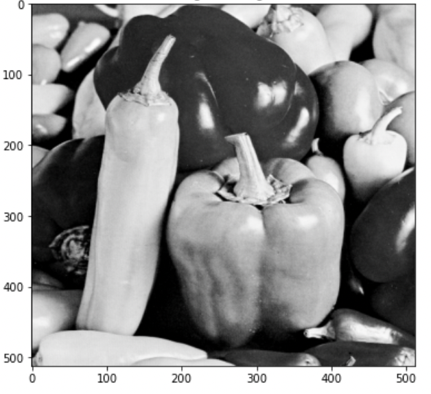
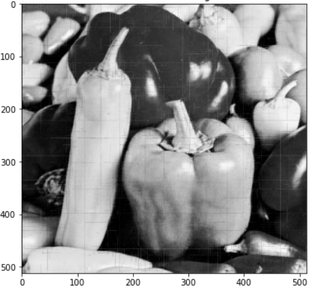
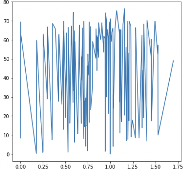
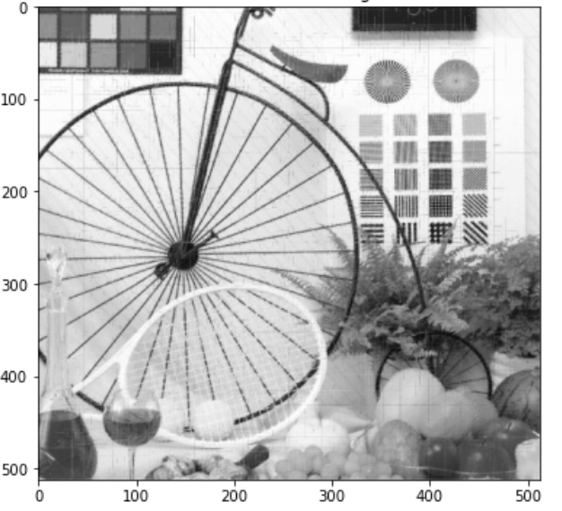
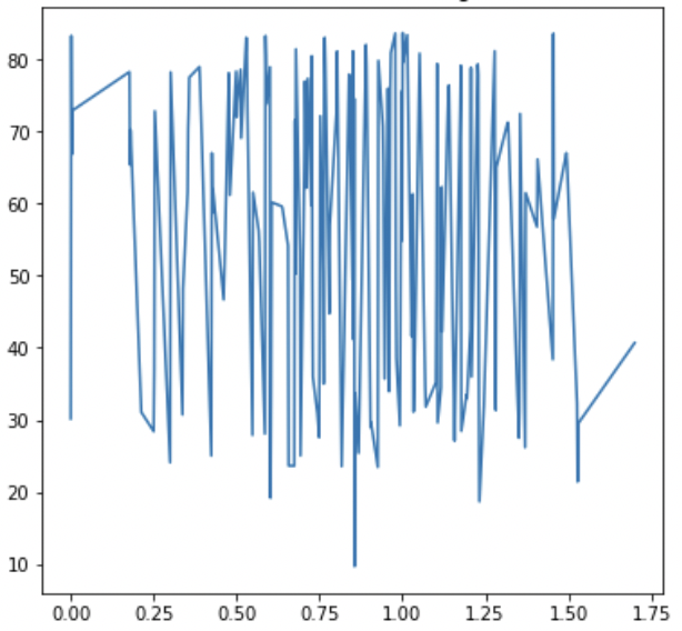
Figure 1: Original image (left column), reconstructed image (middle column), and associated K-outer function $g$ (right column)

Next we present a few examples of smooth functions whose $K$-outer functions may not be Lipschitz continuous in Figure 2. Note that the reconstructed functions are very noisy, in fact they are too noisy to believe that the implementation of the KST can be useful. In order to see that these noisy functions are indeed the original functions, we applied a penalized least squares method based on bivariate spline method (to be explained later in the paper). That is, after denoising, the reconstructed functions are very close to the exact original functions as shown in Figure 2. That is, the denoising method is successful which motivates us to adopt this approach to approximate any continuous functions.

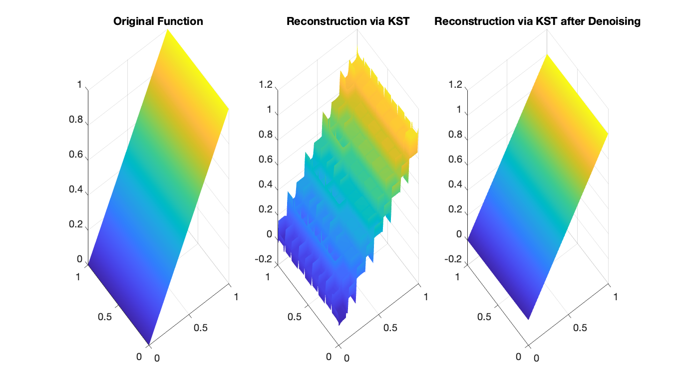
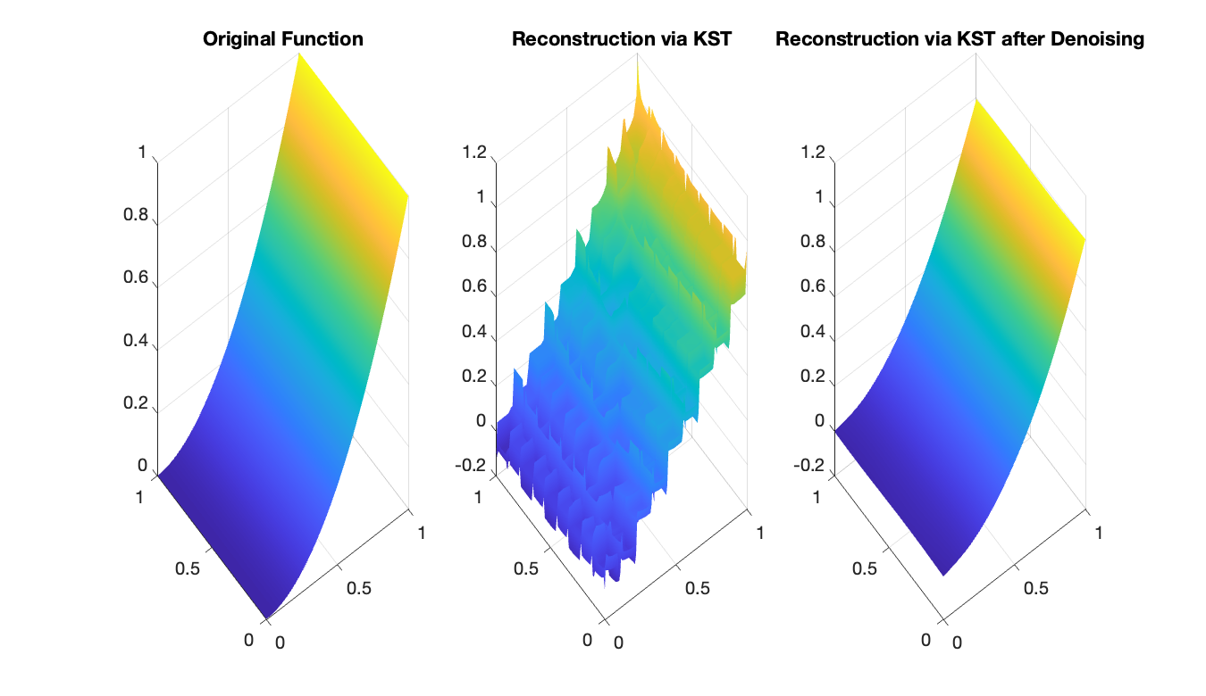
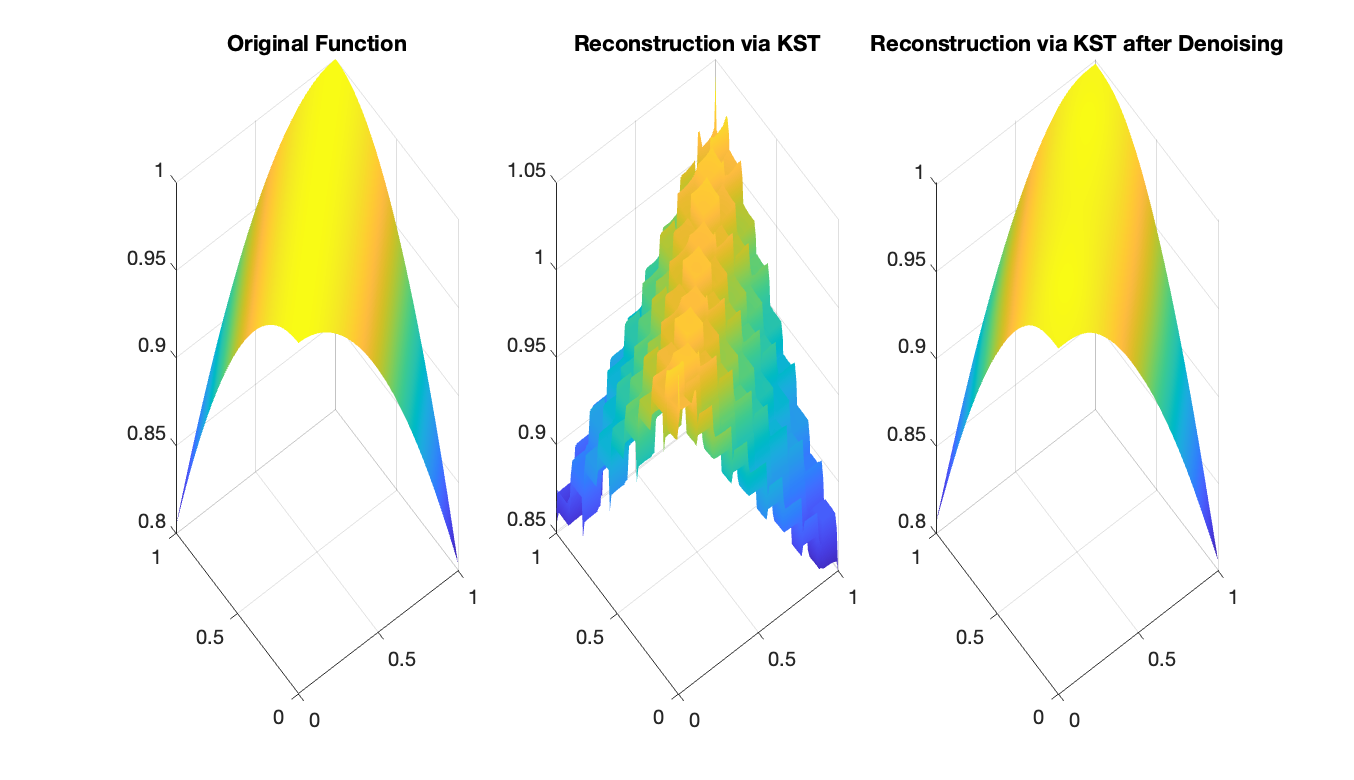
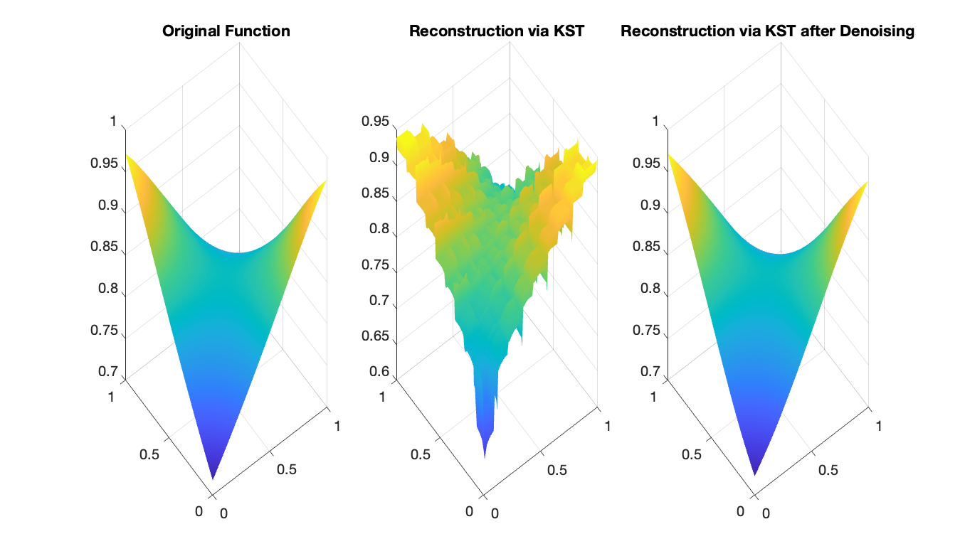
Figure 2: Top left: reconstruction of $f(x,y)=x$. Top right: reconstruction of $f(x,y)=x^{2}$. Bottom left: reconstruction of $f(x,y)=\cos(2(x-y)/\pi)$. Bottom right: reconstruction of $f(x,y)=\sin(1/(1+(x-0.5)(y-0.5)))$.

3.1 KB-splines

To this end, we first use standard uniform B-splines to form some subclasses of K-Lipschitz continuous functions. Let $\triangle_{n}=\{0=t_{1}<t_{2}<\cdots<t_{dn}<d\}$ be a uniform partition of interval $[0,d]$ and let $b_{n,i}(t)=B_{k}(t-t_{i}),i=1,\cdots,dn$ be the standard B-splines of degree $k$ with $k\geq 1$. For simplicity, we only explain our approach based on linear B-splines for the theoretical aspect while using other B-splines (e.g. cubic B-splines) for the numerical experiments. We define KB-splines by

$$KB_{n,j}(x_{1},\cdots,x_{d})=\sum_{q=0}^{2d}b_{n,j}(\sum_{i=1}^{d}\lambda_{i}\phi_{q}(x_{i})),j=1,\cdots,dn.$$ (24)

It is easy to see that each of these KB-splines defined above is nonnegative. Due to the property of B-splines: $\sum_{i=1}^{dn}b_{n,i}(t)=1$ for all $t\in[0,d]$, we have the following property of KB-splines:

Theorem 8

We have $\sum_{i=1}^{dn}KB_{n,i}(x_{1},\cdots,x_{d})=1$ and hence, $0\leq KB_{n,i}\leq 1$.

• Proof. The proof is immediate by using the fact $\sum_{i=1}^{dn}b_{n,i}(t)=1$ for all $t\in[0,d]$. $\Box$

Remark 1

The property in Theorem 8 is called the partition of unit which makes the computation stable. We note that a few of these $dn$ KB-splines will be zero since $0<\lambda_{i}\leq 1$ and $\min\{\lambda_{i},i=1,\cdots,d\}<1$. The number of zero KB-splines is dependent on the choice of $\lambda_{i}$, $i=1,\cdots,d$.

Another important result is that these KB-splines are linearly independent.

Theorem 9

The nonzero KB-splines $\{KB_{n,j}\neq 0,j=1,\cdots,dn\}$ are linearly independent.

• Proof. Suppose there are $c_{j}$, $j=1,2,\cdots,dn$ such that $\sum_{j=1}^{dn}c_{j}KB_{n,j}(x_{1},\cdots,x_{d})=0$ for all $(x_{1},\cdots,x_{d})\in[0,1]^{d}$. Then we want to show $c_{j}=0$ for all $j=1,2,\cdots,dn$. Let us focus on the case $d=2$ as the proof for general case $d$ is similar. Suppose $n>0$ is a fixed integer and we use the notation $z_{q}=\sum_{i=1}^{2}\lambda_{i}\phi_{q}(x_{i})$ as above. Then based on the graphs of $\phi_{q}$ in Figure 3, we can choose $x_{1}=\delta$ and $x_{2}=0$ with $0<\delta\leq 1$ small enough such that $KB_{n,j}(x_{1},0)=\sum_{q=0}^{4}b_{j}(z_{q}(\delta,0))=0$ for all $j=3,4,\cdots,2n$. Therefore in order to show the linear independence of $KB_{n,j},j=1,2,\cdots,2n$, it is suffices to show $\sum_{j=1}^{2}c_{j}KB_{n,j}(x_{1},x_{2})=0$ implies $c_{1}=c_{2}=0$. Let us confine $x_{1}\in[0,\delta]$ and $x_{2}=0$. Then we have

  $$0 =c_{1}KB_{n,1}(x_{1},x_{2})+c_{2}KB_{n,2}(x_{1},x_{2})=c_{1}(\sum_{q=0}^{4}b_{1}(z_{q}))+c_{2}(\sum_{q=0}^{4}b_{2}(z_{q}))$$

  $$=c_{1}(\sum_{q=0}^{4}b_{1}(z_{q}))+c_{2}(5-\sum_{q=0}^{4}b_{1}(z_{q}))=(c_{1}-c_{2})(\sum_{q=0}^{4}b_{1}(z_{q}))+5c_{2},$$

  where we have used the fact that $b_{1}(x)+b_{2}(x)=1$ over $[0,1/n]$. Since $c_{2}$ is constant, and $\sum_{q=0}^{4}b_{1}(z_{q})$ is not constant when $x_{1}$ varies between $0$ and $\delta$, we must have $c_{1}=c_{2}$. Hence $c_{2}=0$ and therefore $c_{1}=0$.

  

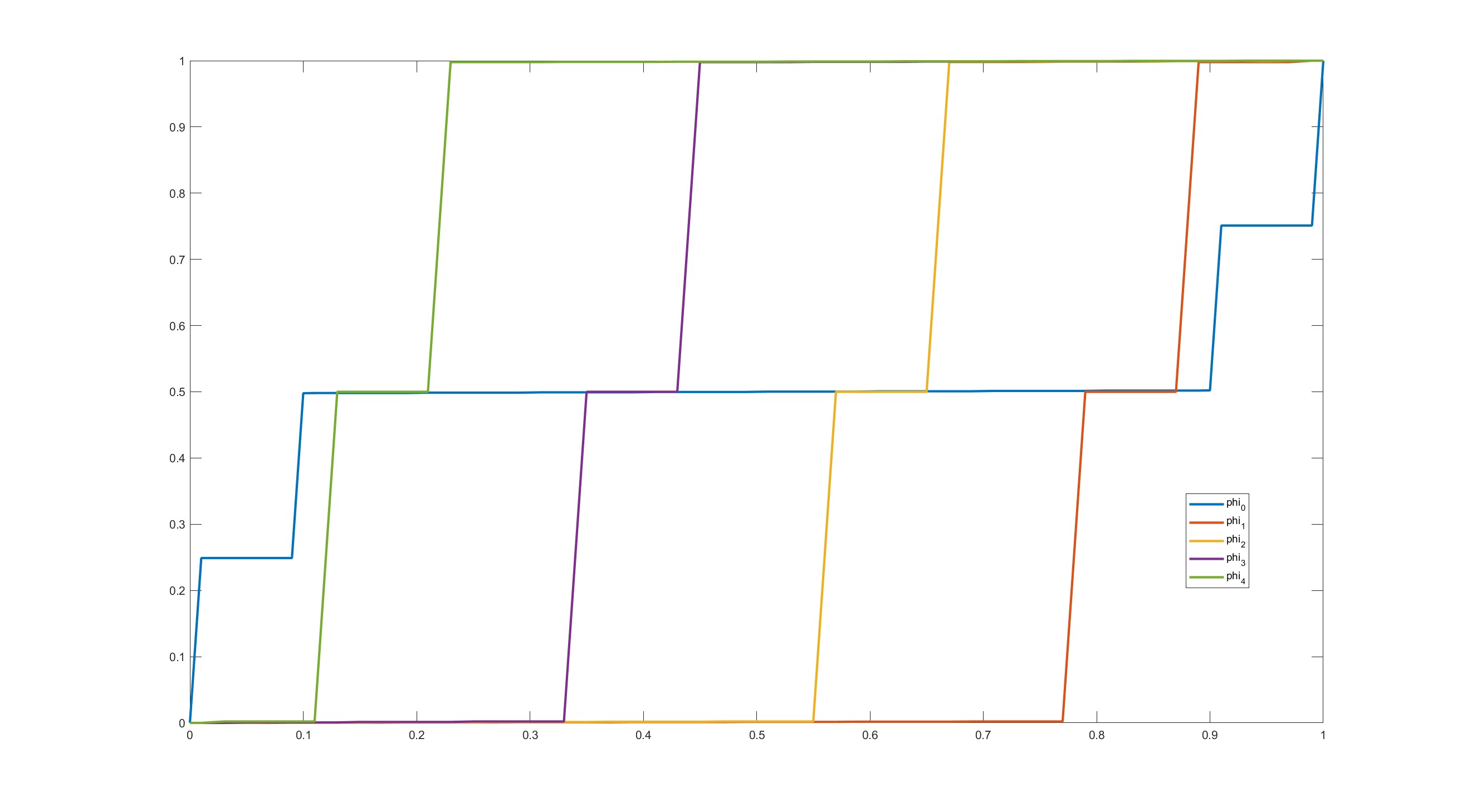
  Figure 3: $\phi_{q}$, $q=0,1,2,3,4$, in the 2D setting.

In the same fashion, we can choose $\tilde{x}_{1}$ and $\tilde{\delta}$ such that $KB_{n,j}=\sum_{q=0}^{4}b_{j}(z_{q}(\tilde{x}_{1},0))=0$ for all $j=1,2,\cdots,2n$ except for $j=k,k+1$. By the similar argument as above, we have $c_{k}=c_{k+1}=0$. By varying $k$ between $1$ and $2n$, we get $c_{j}=0$ for all $j=1,2,\cdots,n$. $\Box$

Since $\hbox{span}\{b_{n,i},i=1,\cdots,nd\}$ will be dense in $C[0,d]$ when $n\to\infty$, we can conclude that $\hbox{span}\{KB_{n,j},j=1,\cdots,nd\}$ will be dense in $C([0,1]^{d})$. That is, we have

Theorem 10

The KB-splines $KB_{n,j}(x_{1},\cdots,x_{d}),j=1,\cdots,nd$, are dense in $C([0,1]^{d})$ when $n\to\infty$.

• Proof. For any continuous function $f\in C([0,1]^{d})$, let $g_{f}\in C[0,d])$ be the K-outer function of $f$. For any $\epsilon>0$, there is an integer $n>0$ and a spline $S_{g_{f}}\in\hbox{span}\{b_{n,i},i=1,\cdots,dn\}$ such that

  $$\|g_{f}(t)-S_{g_{f}}(t)\|_{\infty}\leq\epsilon/(2d+1)$$

  for all $t$. Writing $S_{g_{f}}(t)=\sum_{i=1}^{dn}c_{i}(f)b_{n,i}(t)$, we have

  $$|f(x_{1},\cdots,x_{d})-\sum_{i=1}^{dn}c_{i}(f)KB_{n,i}(x_{1},\cdots,x_{d})|$$

  $$= |\sum_{q=0}^{2d}g(z_{q}(x_{1},\cdots,x_{d}))-\sum_{i=1}^{dn}c_{i}(f)\sum_{q=0}^{2d}b_{n,i}(z_{q}(x_{1},\cdots,x_{d}))|$$

  $$\leq \sum_{q=0}^{2d}|g(z_{q}(x_{1},\cdots,x_{d}))-S_{g_{f}}(z_{q}(x_{1},\cdots,x_{d}))|\leq(2d+1)\epsilon/(2d+1)=\epsilon.$$

  This completes the proof. $\Box$

3.2 LKB-splines

However, in practice, the KB-splines obtained in (24) are very noisy due to any implementation of $\phi_{q}$’s as we have explained before that the functions $z_{q},q=0,\cdots,2d$, like Peano’s curve. One has no way to have an accurate implementation. As demonstrated before, our denoising method can help. We shall call LKB-splines after denoising KB-splines.

Let us explain a multivariate spline method for denoising for $d=2$ and $d=3$. In general, we can use tensor product B-splines for denoising for any $d\geq 2$ which is the similar to what we are going to explain below. For convenience, let us consider $d=2$ and let $\triangle$ be a triangulation of $[0,1]^{2}$. For any degree $D\geq 1$ and smoothness $r\geq 1$ with $r<D$, let

$$S^{r}_{D}(\triangle)=\{s\in C^{r}([0,1]^{2}):s|_{T}\in\mathbb{P}_{D},T\in\triangle\}$$ (25)

be the spline space of degree $D$ and smoothness $r$ with $D>r$. We refer to [36] for a theoretical detail and [2] for a computational detail. For a given data set $\{(x_{i},y_{i},z_{i}),i=1,\cdots,N\}$ with $(x_{i},y_{i})\in[0,1]^{2}$ and $z_{i}=f(x_{i},y_{i})+\epsilon_{i},i=1,\cdots,N$ with noises $\epsilon_{i}$ which may not be very small, the penalized least squares method (cf. [34] and [37]) is to find

$$\min_{s\in S^{1}_{5}(\triangle)}\sum_{i=1,\cdots,N}|s(x_{i},y_{i})-z_{i}|^{2}+\lambda{\cal E}_{2}(s)$$ (26)

with $\lambda\approx 1$, where ${\cal E}_{2}(s)$ is the thin-plate energy functional defined as follows.

$${\cal E}_{2}(s)=\int_{\Omega}|\frac{\partial^{2}}{\partial x^{2}}s|^{2}+2|\frac{\partial^{2}}{\partial x\partial y}s|^{2}+|\frac{\partial^{2}}{\partial y^{2}}s|^{2}.$$ (27)

Multivariate splines have been studied for several decades and they have been used for data fitting (cf. [34], [37], and [38] and [71]), numerical solution of partial differential equations (see, e.g. [35]). and data denoising (see, e.g. [38]).

We now explain that the penalized least squares method can produce a good smooth approximation of the given data. For convenience, let $S_{f,\epsilon}$ be the minimizer of (26) and write $\|f\|_{\cal P}=\sqrt{\frac{1}{N}\sum_{i=1}^{N}|f(x_{i},y_{i})|^{2}}$ is the rooted mean squares (RMS). If $f\in C^{2}([0,1]^{2})$, we have the following

Theorem 11

Suppose that $f$ is twice differentiable over $[0,1]^{2}$. Let $S_{f,\epsilon}$ be the minimizer of (26). Then we have

$$\|f-S_{f,\epsilon}\|_{\cal P}\leq C\|f\|_{2,\infty}|\triangle|^{2}+2\|\epsilon\|_{\cal P}+\sqrt{\lambda{\cal E}_{2}(f)}$$ (28)

for a positive constant $C$ independent of $f$, degree $d$, and triangulation $\triangle$.

To prove the above result, let us recall the following minimal energy spline $S_{f}\in S^{1}_{5}(\triangle)$ of data function $f$: letting $\triangle$ be a triangulation of $[0,1]^{2}$ with vertices $(x_{i},y_{i}),i=1,\cdots,N$, $S_{f}$ is the solution of the following minimization:

$$\min_{S_{f}\in S^{1}_{5}(\triangle)}\{{\cal E}_{2}(S_{f}):\quad S_{f}(x_{i},y_{i})=f(x_{i},y_{i}),(x_{i},y_{i}),i=1,\cdots,N.\}$$ (29)

Then it is known that $S_{f}$ approximates $f$ very well if $f\in C^{2}([0,1]^{2})$. We have

Theorem 12 (von Golitschek, Lai and Schumaker, 2002([70]))

Suppose that $f\in C^{2}([0,1]^{2})$. Then

$$\|S_{f}-f\|_{\infty}\leq C\|f\|_{2,\infty}|\triangle|^{2}$$ (30)

for a positive constant $C$ independent of $f$ and $\triangle$, where $\|f\|_{2,\infty}$ denotes the maximum norm of the second order derivatives of $f$ over $[0,1]^{2}$ and $\|S_{f}-f\|_{\infty}$ is the maximum norm of $S_{f}-f$ over $[0,1]^{2}$.

• Proof.[ of Theorem 11] Recall that $S_{f,\epsilon}$ is the minimizer of (26). We now use $S_{f}$ to have

  $$\|f-S_{f,\epsilon}\|_{\cal P} \leq \|z-S_{f,\epsilon}\|_{\cal P}+\|\epsilon\|_{\cal P}\leq\sqrt{\|z-S_{f,\epsilon}\|^{2}_{\cal P}+\lambda{\cal E}_{2}(S_{f,\epsilon})}+\|\epsilon\|_{\cal P}$$

  $$\leq \sqrt{\|z-S_{f}\|^{2}_{\cal P}+\lambda{\cal E}_{2}(S_{f})}+\|\epsilon\|_{\cal P}\leq\|f-S_{f}\|_{\cal P}+2\|\epsilon\|_{\cal P}+\sqrt{\lambda{\cal E}_{2}(f)}$$

  $$\leq C\|f\|_{2,\infty}|\triangle|^{2}+2\|\epsilon\|_{\cal P}+\sqrt{\lambda{\cal E}_{2}(f)},$$

  where we have used a fact that ${\cal E}_{2}(S_{f})\leq{\cal E}_{2}(f)$ which can be found in [70]. These complete the theorem of this section. $\Box$

If $f$ is $C^{2}$ smooth, then $S_{f,\epsilon}$ will be a good approximation of $f$ when the size $|\triangle|$ of triangulation is small, the thin plate energy ${\cal E}_{2}(f)$ with $\lambda>0$ is small, and the noises $\|\epsilon\|_{\cal P}$ is small even though a few individual noises $\epsilon_{i}$ can be large. Note also that $\epsilon$ can be made small by increasing the accuracy of the implementaion of $\phi_{q}$.

Now let us illustrate some examples of KB-splines and LKB-splines in Figure 4. One can see that the KB-splines are continuous but not smooth functions at all, while the LKB-splines are. With these LKB-splines in hand, we can approximate high dimensional continuous functions accurately. Let us report our numerical results in the next section.

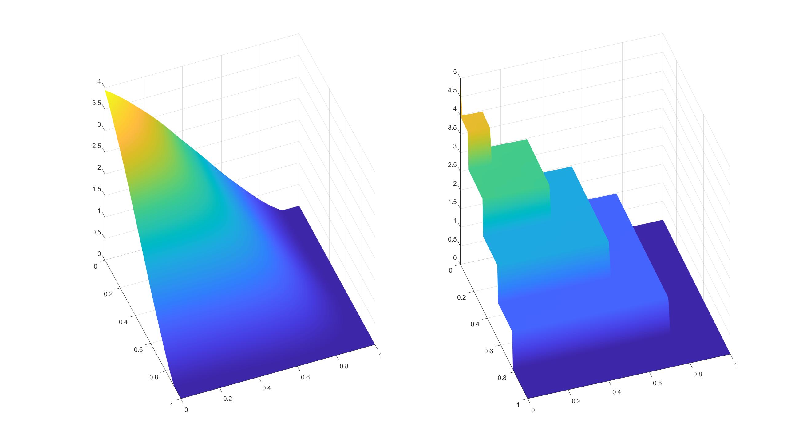
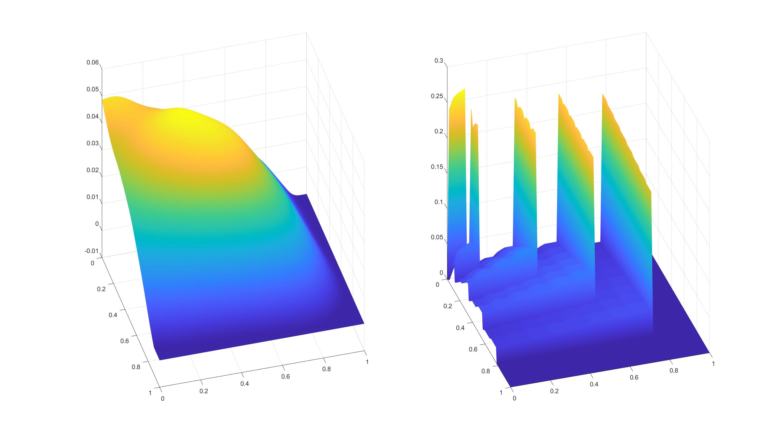
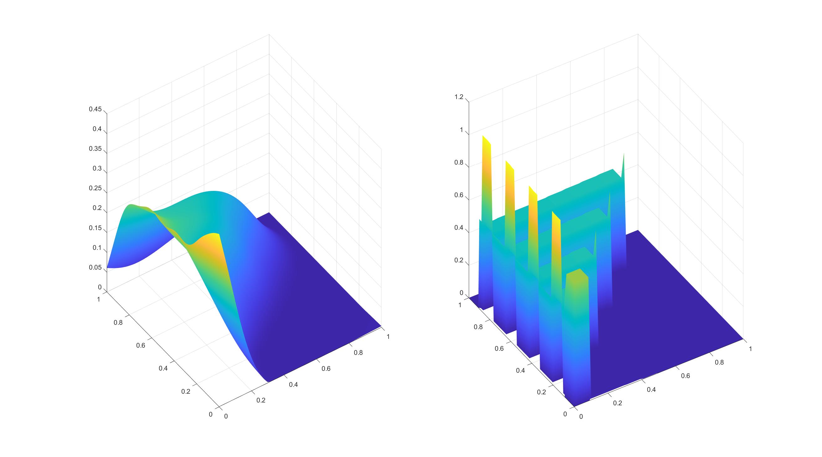
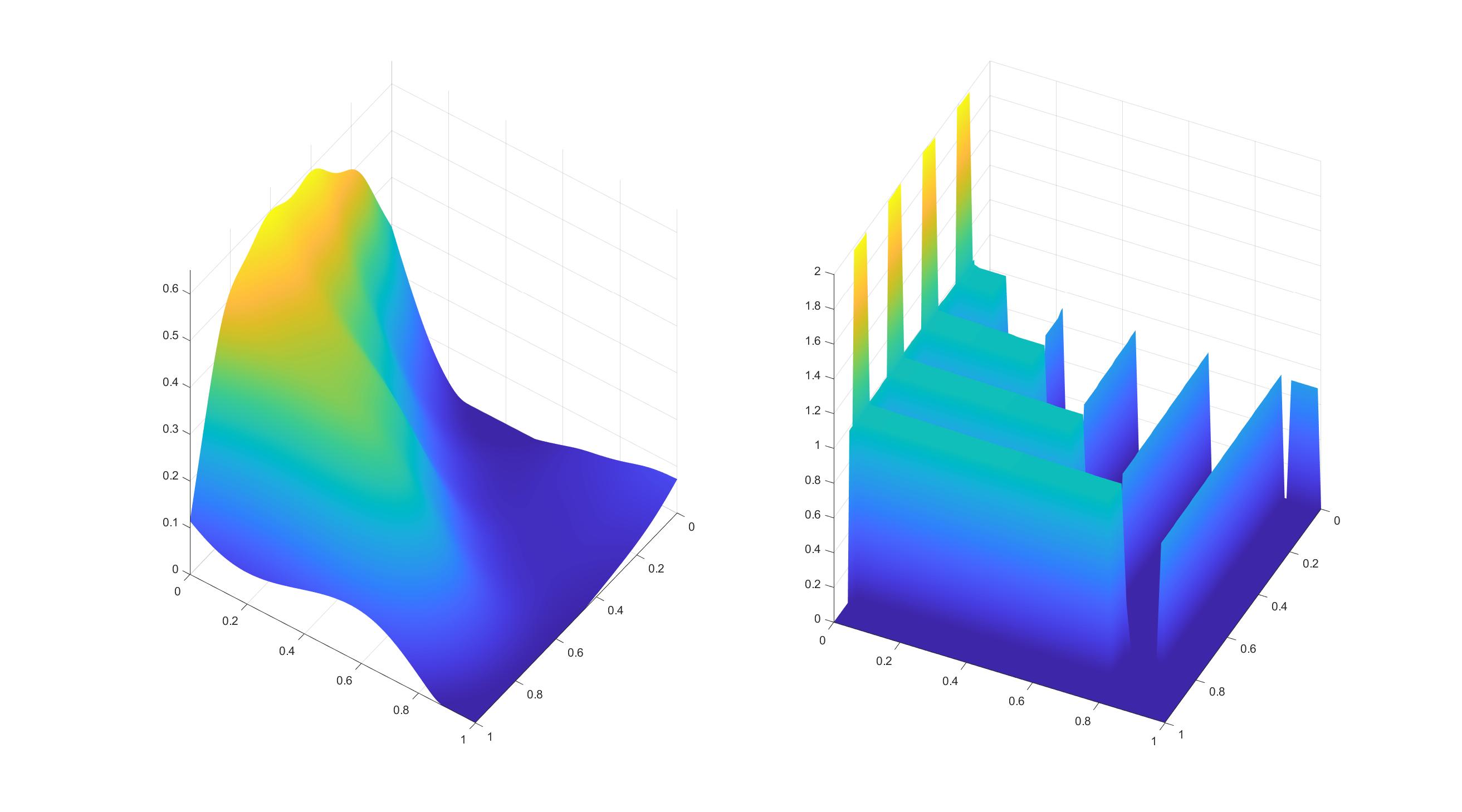
Figure 4: Examples of LKB-splines (first and third columns) which are the smoothed version of the corresponding KB-splines (second and fourth columns).

4 Numerical Approximation by LKB-splines

In this section, we will first demonstrate numerically that LKB-splines can approximate general continuous functions well based on $O(n^{d})$ equally-spaced sampled data locations. Then we use the matrix cross approximation technique to show that there are at most $O(nd)$ locations among those $O(n^{d})$ locations are pivotal. Therefore, we only need the function values at those pivotal locations in order to achieve a reasonable good approximation.

4.1 Numerical results based on $O(n^{d})$ data points

Let us design numerical experiments to demonstrate the power of LKB-splines for approximating functions in $C([0,1]^{d})$. We choose $41^{d}$ equally-spaced points ${\bf x}_{i}\in[0,1]^{d}$. For any continuous function $f\in C([0,1]^{d})$, we use the function values at these data locations to find an approximation $F_{n}=\sum_{j=1}^{dn}c_{j}LKB_{n,j}$ by using discrete least squares (DLS) method. In other words, we solve the following minimization problem:

$$\min_{c_{j}}\|f-\sum_{j=1}^{dn}c_{j}LKB_{n,j}\|_{\cal P},$$ (31)

where $\|f\|_{\cal P}$ is the RMS semi-norm based on the function values $f$ over these $41^{d}$ sampled data points in $[0,1]^{d}$. We shall report the accuracy $\|f-F_{n}(f)\|_{\cal PP}$, where $\|f\|_{\cal PP}$ is the RMS semi-norm based on $101^{d}$ function values. The current computational power enables to do the numerical experiments for $d=2$ with $n=100,200,\cdots,10,000$ and for $d=3$ with $n=100,200,\cdots,1000$.

For $d=2$, we choose the following 10 testing functions across different families of continuous functions to check the computational accuracy.

$$f_{1} = (1+2x+3y)/6;f_{2}=(x^{2}+y^{2})/2;f_{3}=xy;$$

$$f_{4} = (x^{3}+y^{3})/2;f_{5}=1/(1+x^{2}+y^{2});$$

$$f_{6} = \cos(1/(1+xy));f_{7}=\sin(2\pi(x+y));$$

$$f_{8} = \sin(\pi x)\sin(\pi y);f_{9}=\exp(-x^{2}-y^{2});$$

$$f_{10} = \max(x-0.5,0)\max(y-0.5,0);$$

For $d=3$, we choose the following 10 testing functions across different families of continuous functions to check the computational accuracy. The computational results are reported in Tables 1 and 2 (those columns associated with $41^{3}$).

$$f_{1} = (1+2x+3y+4z)/10;f_{2}=(x^{2}+y^{2}+z^{2})/3;f_{3}=(xy+yz+zx)/3;$$

$$f_{4} = (x^{3}y^{3}+y^{3}z^{3})/2;f_{5}=(x+y+z)/(1+x^{2}+y^{2}+z^{2});$$

$$f_{6} = \cos(1/(1+xyz));f_{7}=\sin(2\pi(x+y+z));$$

$$f_{8} = \sin(\pi x)\sin(\pi y)\sin(\pi z);f_{9}=\exp(-x^{2}-y^{2}-z^{2});$$

$$f_{10} = \max(x-0.5,0)\max(y-0.5,0)\max(z-0.5,0);$$

Remark 2

The major computational burden for these results Tables 1 and 2 is the denoise of the KB-splines to get LKB-splines which requires a large amount of data points and values as the noises are everwhere over $[0,1]^{d}$. When dimension $d\gg 1$ gets large, one has to use an exponentially increasing number of points and KB-spline values by, say a tensor product spline method for denoising, and hence, the computational cost will suffer the curse of dimensionality. However, the denoising step can be pre-computed once for all the approximation tasks. That is, once we have the LKB-splines, the rest of the computational cost is no more than the cost of solving a least squares problem. We leave the numerical results for $d>3$ in [58].

This shows the power of LKB-splines in approximating general continuous functions. However, the number of data points being sampled in order to achieve such approximation error is $O(n^{d})$. Therefore, when $d$ gets large, we still need exponentially many sampled data. Our final goal in this paper is to reduce this amount of data values. It turns out this goal can be achieved. In fact, we only need at most $O(nd)$ number of sampled data instead of $O(n^{d})$ in order to achieve the same order of approximation accuracy. Let us further explain our study in the next subsection.

Table 1: RMSEs (computed based on $101^{2}$ equally-spaced locations) of the DLS fitting (31) based on $41^{2}$ equally-spaced location and pivotal location in 2D.

	$n=100$		$n=1000$		$n=10000$
# sampled data	$41^{2}$	54	$41^{2}$	105	$41^{2}$	521
$f_{1}$	1.67e-05	2.60e-05	5.79e-06	1.02e-05	5.14e-07	1.21e-06
$f_{2}$	4.19e-04	8.92e-04	1.17e-04	2.61e-04	2.83e-05	6.62e-05
$f_{3}$	1.09e-04	2.19e-04	3.57e-05	7.46e-05	2.20e-05	5.67e-05
$f_{4}$	7.67e-04	1.70e-03	2.10e-04	5.11e-04	4.99e-05	1.11e-04
$f_{5}$	2.28e-04	5.04e-04	6.69e-05	1.47e-04	1.93e-05	4.08e-05
$f_{6}$	2.52e-04	6.51e-04	7.97e-05	1.94e-04	1.43e-05	2.73e-05
$f_{7}$	7.05e-02	1.32e-01	7.80e-03	2.25e-02	1.30e-03	3.30e-03
$f_{8}$	1.50e-03	2.29e-03	3.73e-04	1.01e-03	1.69e-04	4.37e-04
$f_{9}$	3.49e-04	7.97e-04	8.25e-05	1.98e-04	2.48e-05	5.52e-05
$f_{10}$	2.02e-03	3.79e-03	7.77e-04	1.82e-03	1.68e-04	4.10e-04

Table 2: RMSEs (computed based on $101^{3}$ equally-spaced locations) of the DLS fitting (31) based on $41^{3}$ equally-spaced location and pivotal location in 3D.

	$n=100$		$n=300$		$n=1000$
# sampled data	$41^{3}$	178	$41^{3}$	331	$41^{3}$	643
$f_{1}$	8.27e-06	2.25e-05	1.51e-06	4.20e-06	3.62e-07	7.48e-07
$f_{2}$	4.42e-05	1.68e-04	8.14e-06	2.18e-05	1.87e-06	4.11e-06
$f_{3}$	1.24e-05	3.79e-05	3.77e-06	9.41e-06	1.22e-06	2.53e-06
$f_{4}$	2.93e-04	5.60e-04	1.43e-04	2.55e-04	1.16e-04	2.63e-04
$f_{5}$	1.31e-04	3.46e-04	9.09e-05	1.66e-04	6.61e-05	1.20e-04
$f_{6}$	1.24e-04	3.22e-04	7.02e-05	1.34e-04	5.18e-05	1.09e-04
$f_{7}$	1.65e-02	5.29e-02	1.15e-02	1.71e-02	1.10e-02	1.85e-02
$f_{8}$	2.47e-03	8.28e-03	9.60e-04	1.94e-03	7.20e-04	1.19e-03
$f_{9}$	1.43e-04	3.84e-04	1.14e-04	2.01e-04	9.84e-05	3.95e-04
$f_{10}$	3.21e-04	9.74e-04	2.31e-04	4.00e-04	2.04e-04	3.91e-04

4.2 The pivotal data locations for breaking the curse of dimensionality

For convenience, let us use $M$ to indicate the data matrix associated with the discrete least squares problem (31). In other words, for $1\leq j\leq dn$, the $j$th column $M(:,j)$ consists of $\{LKB_{n,j}(\mathbf{x}_{i})\}$ where $\mathbf{x}_{i}\in[0,1]^{d}$ are those $41^{d}$ equally-spaced sampled points in 2D or 3D. Clearly, the experiment above requires $41^{d}$ data values which suffers from the curse of dimensionality. However, we in fact do not need such many data values. The main reason is that the data matrix $M$ has many zero columns or near zero columns due to the fact that for many $i=1,\cdots,nd$, the locations from $41^{d}$ equally-spaced points do not fall into the support of linear B-splines $b_{n,i}(t)$, $t\in[0,d]$, based on the map $z_{q}$. The structures of $M$ are shown in Figure 5 for the case of $n=1000$ when $d=2$.

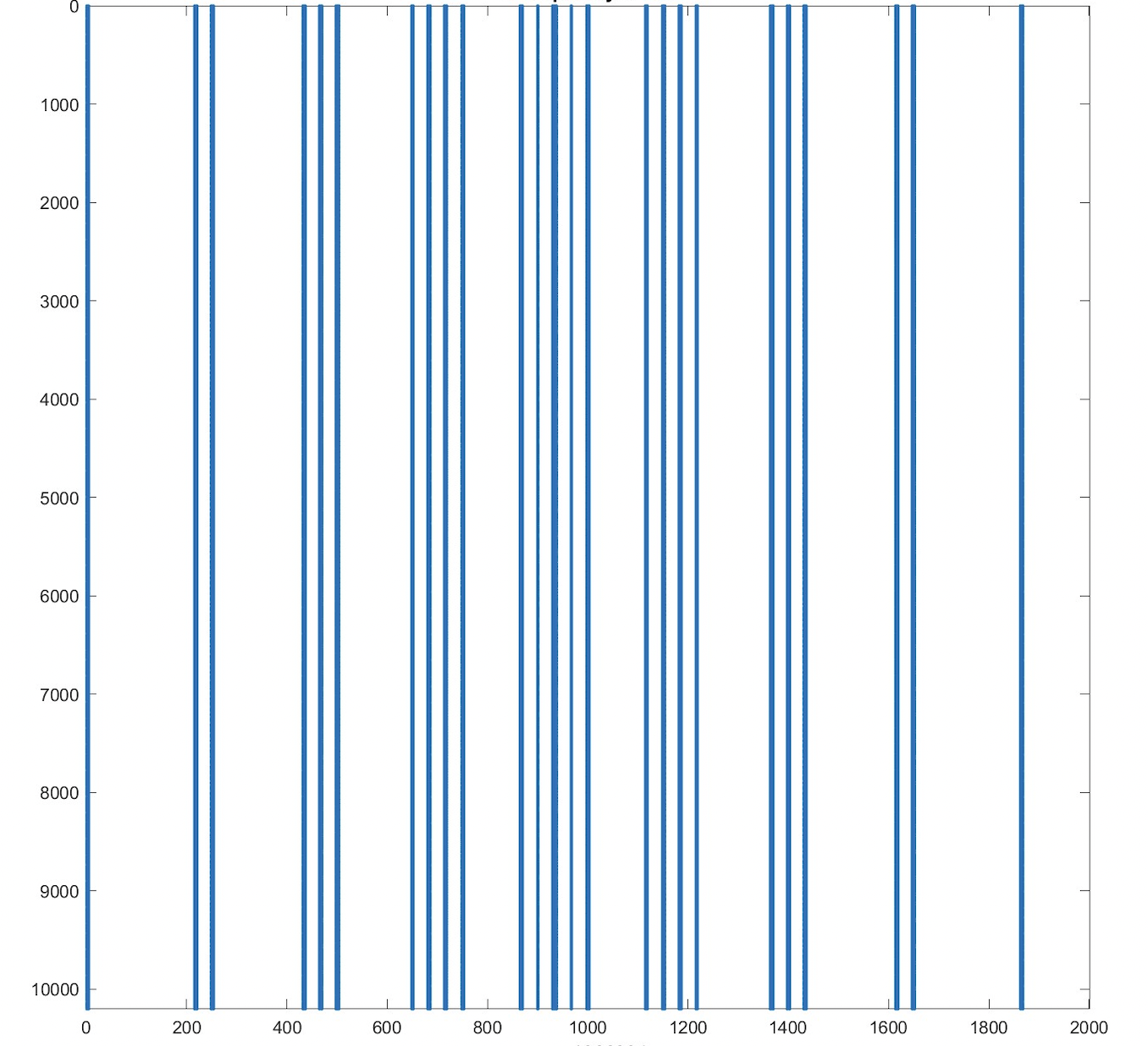
Figure 5: The sparsity pattern of data matrix for $n=1000$.

That is, there are many columns in $M$ whose entries are zero or near zero. Therefore, there exists a sparse solution to the discrete least squares fitting problem. We adopt the well-known orthogonal matching pursuit (OMP) (cf. e.g. [39]) to find a solution. For convenience, let us explain the sparse solution technique as follows. Over those $41^{d}$ points ${\bf x}_{i}\in[0,1]^{d}$, the columns in the matrix

$$M=[LKB_{n,j}({\bf x}_{i})]_{i=1,\cdots,41^{d},j=1,\cdots,dn}$$ (32)

are not linearly independent. Let $\Phi$ be the normalized matrix of $M$ in (32) and ${\bf b}=[f({\bf x}_{i})],i=1,\cdots,41^{d}$. Write ${\bf c}=(c_{1},\cdots,c_{dn})^{\top}$, we look for

$$\min\|{\bf c}\|_{0}:\Phi{\bf c}={\bf b}$$ (33)

where $\|{\bf c}\|_{0}$ stands for the number of nonzero entries of ${\bf c}$. See many numerical methods in ([39]). The near zero columns in $\Phi$ also tell us that the data matrix associated with (31) of size $41^{d}\times dn$ is not full rank $r<dn$. The LKB-splines associated with these near zero columns do not play a role. Therefore, we do not need all $dn$ LKB-splines. Furthermore, let us continue to explain that many data locations among these $41^{d}$ locations do not play an essential role.

To this end, we use the so-called matrix cross approximation (see [23], [24], [48], [20], [25], [1] and the literature therein). Let $r\geq 1$ be a rank of the approximation. It is known (cf. [23]) that when $M_{I,J}$ of size $r\times r$ has the maximal volume among all submatrices of $M$ of size $r\times r$, we have

$$\|M-M_{:,J}M_{I,J}^{-1}M_{I,:}\|_{C}\leq(1+r)\sigma_{r+1}(M),$$ (34)

where $\|\cdot\|_{C}$ is the Chebyshev norm of matrix and $\sigma_{r+1}(M)$ is the $r+1$ singular value of $M$, $M_{I,:}$ is the row block of $M$ associated with the indices in $I$ and $M_{:,J}$ is the column block of $M$ associated with the indices in $J$. The volume of a square matrix $A$ is the absolute value of the determinant of $A$.

One mainly needs to find a submatrix $M_{I,J}$ of $M$ such that $M_{I,J}$ has the maximal volume among all $r\times r$ submatrices of $M$. In practice, we use the concept called dominant matrix to replace the maximal volume. There are several algorithms, e.g. maxvol algorithm, available in the literature (cf. [24]). Recall that originally we need to solve the DLS problem $M{\bf x}_{f}\approx{\bf f}=[{\bf f}_{I};{\bf f}_{I^{c}}]$. However, these greedy based maxvol algorithms enable us to find a good submatrix $M_{I,J}$ and solve a much simpler discrete least squares problem $M_{I,J}\widehat{{\bf x}}\approx{\bf f}_{I}$. According to Theorem 8 in [1], that $\widehat{{\bf x}}$ is a good approximation of ${\bf x}_{f}$. Let us call the data locations associated with row indices $I$ the pivotal data locations. The pivotal data locations are shown in Figure 6. It is worthwhile to point out that such a set of pivotal locations is only dependent on the partition between $[0,d]$ when numerically build KB-splines, the sampled data when constructing LKB-splines, and the smoothing parameters for converting KB-splines to LKB-splines. However, such set of pivotal locations is independent of the target function to approximate.

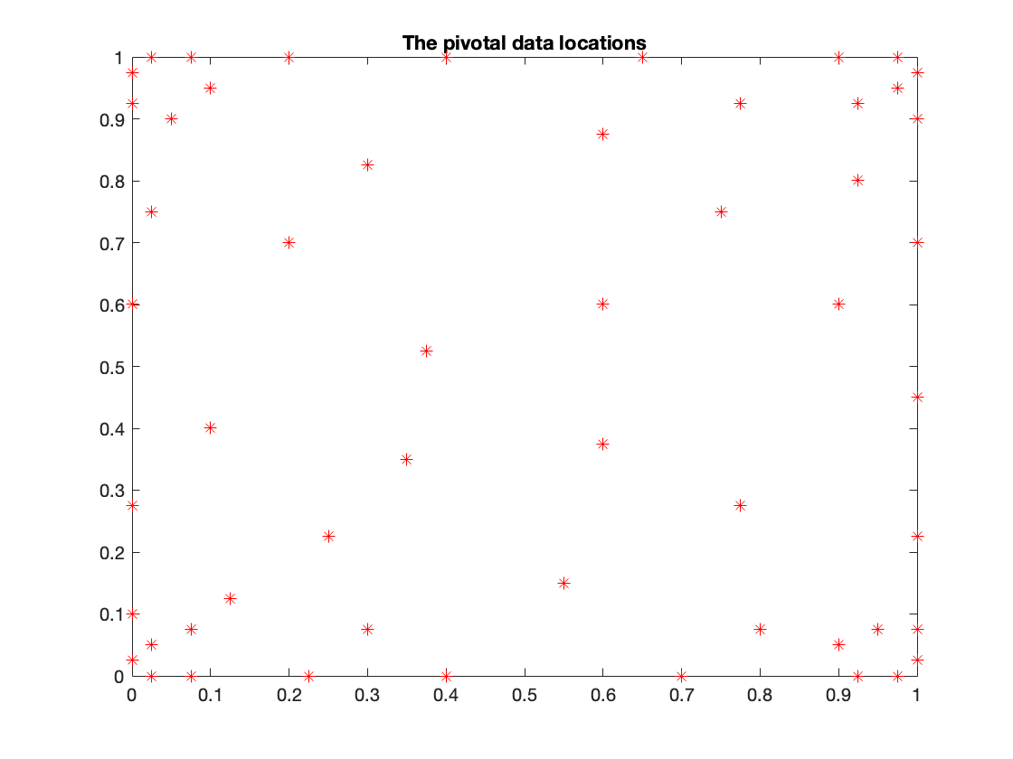
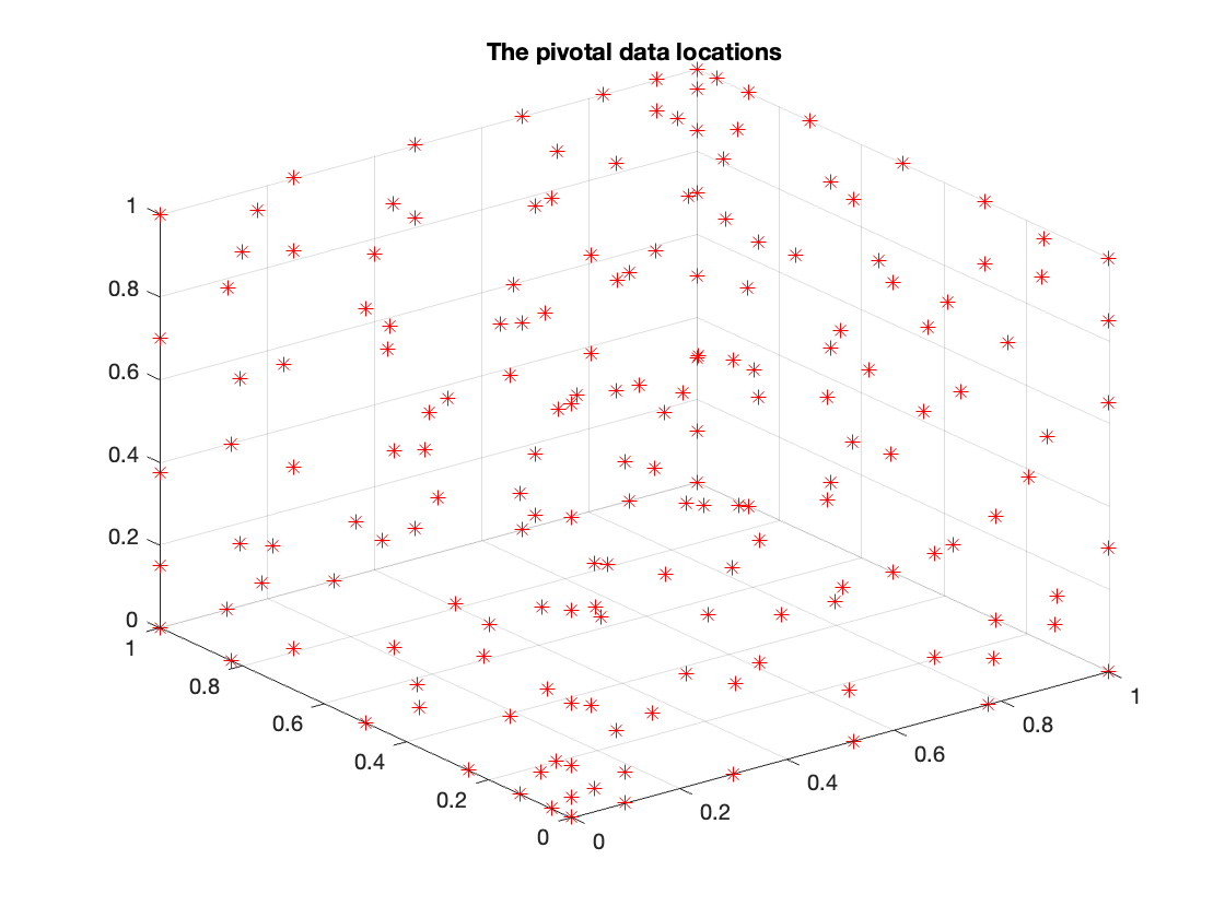
Figure 6: Pivotal data at 54 locations (selected from $41^{2}$ equally-spaced locations) in 2D and 178 locations (selected from $41^{3}$ equally-spaced locations) in 3D for $n=100$.

We now present some numerical results in Table 1 and 2 (those columns associated with $54,105,521$ and $178,331,643$) to demonstrate that the numerical approximation results based on pivotal data locations have the same order as the results based on data locations sampled on the uniform grid. We therefore conclude that the curse of dimensionality for 2D and 3D function approximation can be overcome if we use LKB-splines with pivotal data sets.

We also plot the approximation error of several aforementioned functions based on pivotal data locations against $n$ using log-log scale. The results are shown in Figure 7. It is worthwhile to note that the slopes in these plots are associated with the exponent $\alpha$ in Theorem 6. In other words, if the slope of an convergence plot for a function is smaller than $-1$, then we can numerically conclude that such a function belongs to the class of K-Lipschitz continuous functions. If the slope $\alpha$ satisfies $-1<\alpha<0$, then we can numerically conclude that such a function belongs to the class of K-Hölder continuous functions with the outer function $g$ belongs to $C^{0,\alpha}$. In Figure 8, we plot the number of pivotal locations against $n$, we can see that the number of pivotal locations increasing linearly with $n$, and the increasing rates (slopes) are at most $d$.

$f(x,y)=(x^{3}+y^{3})/2$	$f(x,y)=\sin(2\pi(x+y))$	$f(x,y)=\max(x-0.5,0)\max(y-0.5,0)$
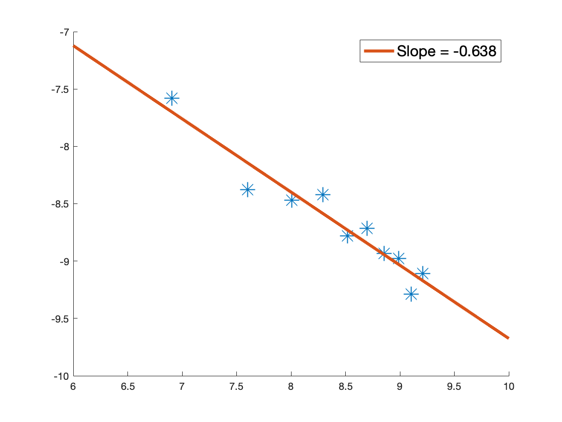
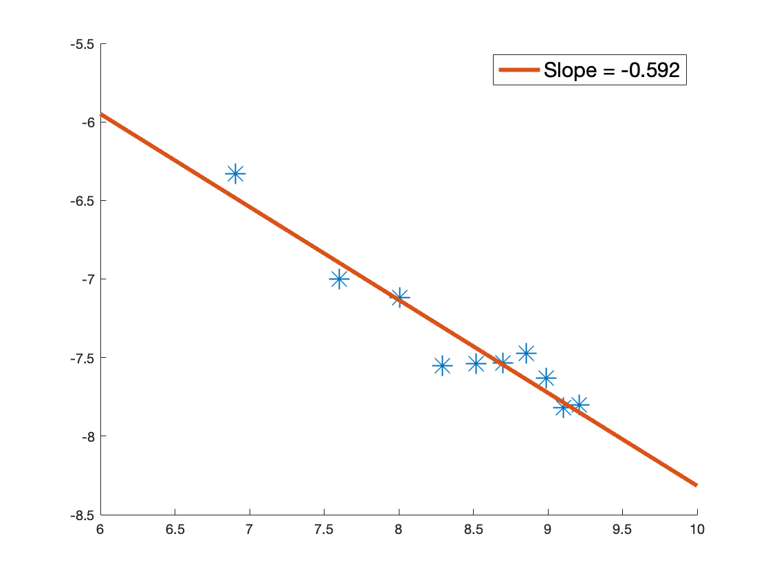
$f(x,y,z)=(1+2x+3y+4z)/10$	$f(x,y,z)=(xy+yz+zx)/3$	$f(x,y)=\sin(\pi x)\sin(\pi y)\sin(\pi z)$

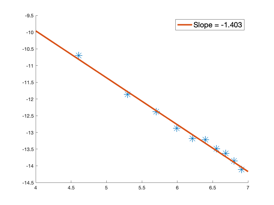
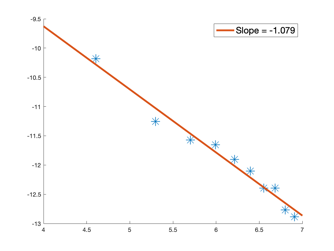
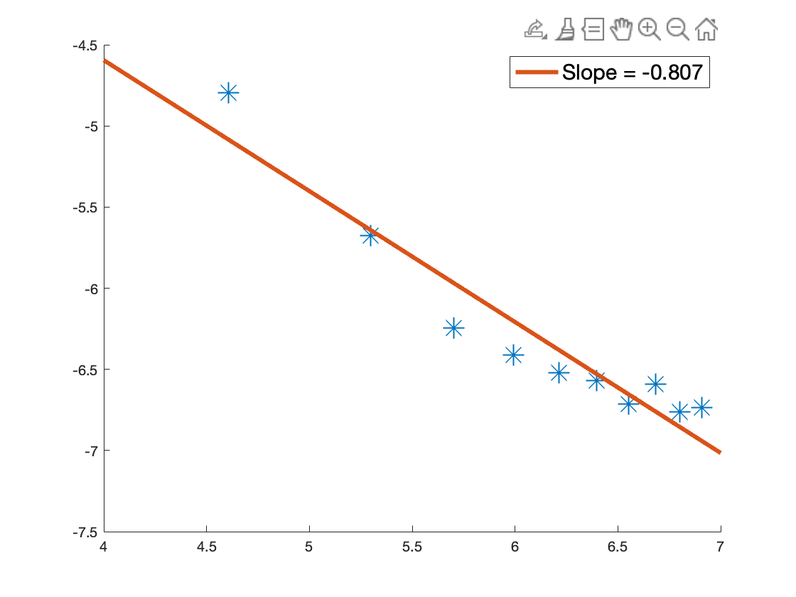
Figure 7: Plot of Convergence Rate using Log-log Scale for Functions in 2D and 3D.

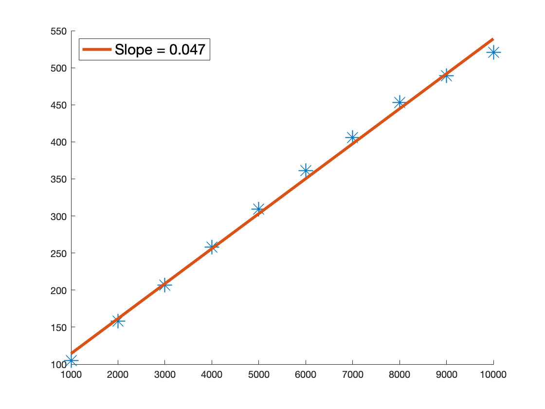
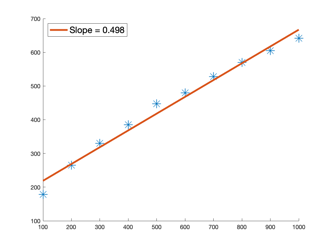
Figure 8: Number of Pivotal Locations (vertical axis) against $n$ (horizontal axia) in 2D (left) and in 3D (right).

Finally, let us end up this section with some important remarks.

Remark 3

The pivotal data set depends on the partition between $[0,d]$ when numerically build KB-splines, the sampled data when constructing LKB-splines, and the smoothing parameters for converting KB-splines to LKB-splines. For example, if we use randomly sampled points instead of equally-space points, or if we use $81\times 81$ equally-spaced points instead of $41\times 41$ equally-spaced points when constructing LKB-splines over $[0,1]^{2}$, then the location of the pivotal data are different and the size of pivotal data set is bigger than the ones shown in Figure 6.

Remark 4

Certainly, there are many functions such as $f(x,y)=\sin(100x)\sin(100y)$ or $f(x,y)=\tanh(100((2x-1)^{2}+(2y-1)^{2}-0.25))$ which the LKB-splines can not approximate well based on the pivotal data sets above. Such highly oscillated functions are hard to approximate even using other methods such as multivariate splines. One indeed needs a lot of the data (points and the function values over the points) to approximate them well. One may also consider to use Fourier basis rather than B-splines basis to approximate such highly oscillated trigonometric functions via KST. We leave it as a future research topic.

Remark 5

To duplicate the experimental results in this paper, we uploaded our MATLAB codes in https://github.com/zzzzms/KST4FunApproximation. In fact, we have tested more than 100 functions in 2D and 3D with pivotal data sets which enables us to approximate these functions very well.

References

- [1] K. Allen, M. -J. Lai, Z. Shen, Maximal volume matrix cross approximation for image compression and least squares solution, submitted, 2023 (https://arxiv.org/abs/2309.17403).
- [2] G. Awanou, M. -J. Lai, P. Wenston, The multivariate spline method for scattered data fitting and numerical solutions of partial differential equations, Wavelets and splines: Athens (2005), 24–74.
- [3] F. Bach, Breaking the curse of dimensionality with convex neural networks, Journal of Machine Learning Research, vol. 18, 2017, 1–53.
- [4] A. R. Barron. Universal approximation bounds for superpositions of a sigmoidal function, IEEE Transactions on Information theory, 39(3):930–945, 1993.
- [5] B J. Braun, An Application of Kolmogorov’s Superposition Theorem to Function Reconstruction in Higher Dimensions, PhD thesis, University of Bonn, 2009.
- [6] B. J. Braun and M. Griebel, On a constructive proof of Kolmogorov’s superposition theorem, Constructive Approximation, 30(3):653–675, 2009.
- [7] D. W. Bryant. Analysis of Kolmogorov’s superposition theorem and its implementation in applications with low and high dimensional data. PhD thesis, University of Central Florida, 2008
- [8] K. Chen, The upper bound on knots in neural networks, arXiv:1611.09448v2 [stat.ML] 30 Nov 2016.
- [9] G. Cybenko, Approximation by Superpositions of a Sigmoidal Function, Math. Control Signals Systems (1989) 2:303–314.
- [10] I. Daubechies, R. DeVore, S. Foucart, B. Hanin, and G. Petrova, Nonlinear Approximation and (Deep) ReLU Networks, Constructive Approximation 55, no. 1 (2022): 127-172.
- [11] R. DeVore, R. Howard, and C. Micchelli, Optimal nonlinear approximation, Manuscripta Mathematica, 63(4):469–478, 1989.
- [12] R. DeVore, B. Hanin, and G. Petrova, Neural Network Approximation, Acta Numerica 30 (2021): 327-444.
- [13] R. Doss, On the representation of continuous functions of two variables by means of addition and continuous functions of one variable. Colloquium Mathematicum, X(2):249–259, 1963.
- [14] Weinan E, Machine Learning and Computational Mathematics, arXiv:2009.14596v1 [math.NA] 23 Sept. 2020.
- [15] Weinan E, Chao Ma and Lei Wu, Barron spaces and the flow-induced function spaces for neural network models, Constructive Approximation 55, no. 1 (2022): 369-406
- [16] Weinan E and Stephan Wojtowytsch, Representation formulas and pointwise properties for Barron functions, Calculus of Variations and Partial Differential Equations 61, no. 2 (2022): 1-37.
- [17] Weinan E and Stephan Wojtowytsch, On the Banach spaces associated with multilayer ReLU networks: Function representation, approximation theory and gradient descent dynamics, https://arxiv.org/abs/2309.17403
- [18] B. L. Friedman, An improvement in the smoothness of the functions in Kolmogorov’s theorem on superpositions. Doklady Akademii Nauk SSSR, 117:1019–1022, 1967.
- [19] Z. Feng, Hilbert’s 13th problem. PhD thesis, University of Pittsburgh, 2010.
- [20] Irina Georgieva and Clemens Hofreithery, On the Best Uniform Approximation by Low-Rank Matrices, Linear Algebra and its Applications, vol.518(2017), Pages 159–176.
- [21] Girosi, F., and Poggio, T. (1989). Representation properties of networks: Kolmogorov’s theorem is irrelevant. Neural Computation, 1(4), 465-469.
- [22] I. Goodfellow, Y. Bengio, A. Courville, Deep Learning, MIT Press, 2016.
- [23] S. A. Goreinov and E. E. Tyrtyshnikov, The maximal-volume concept in approximation by low-rank matrices, Contemporary Mathematics, 208: 47–51, 2001.
- [24] S. A. Goreinov, I. V. Oseledets, D. V. Savostyanov, E. E. Tyrtyshnikov, N. L. Zamarashkin, How to find a good submatrix, in: Matrix Methods: Theory, Algorithms, Applications, (World Scientific, Hackensack, NY, 2010), pp. 247–256.
- [25] N. Kishore Kumar and J. Schneider, Literature survey on low rank approximation of matrices, Journal on Linear and Multilinear Algebra, vol. 65 (2017), 2212–2244.
- [26] M. Hansson and C. Olsson, Feedforward neural networks with ReLU activation functions are linear splines, Bachelor Thesis, Univ. Lund, 2017.
- [27] R. Hecht-Nielsen, Kolmogorov’s mapping neural network existence theorem. In Proceedings of the international conference on Neural Networks, volume 3, pages 11–14. New York: IEEE Press, 1987.
- [28] K. Hornik, Approximation capabilities of multilayer feedforward networks. Neural Networks 4, no. 2 (1991): 251-257.
- [29] B. Igelnik and N. Parikh, Kolmogorov’s spline network. IEEE Transactions on Neural Networks, 14(4):725–733, 2003.
- [30] J. M. Klusowski and Barron, A.R.: Approximation by combinations of ReLU and squared ReLU ridge functions with and controls. IEEE Transactions on Information Theory 64(12), 7649–7656 (2018).
- [31] A. N. Kolmogorov. The representation of continuous functions of several variables by superpositions of continuous functions of a smaller number of variables. Doklady Akademii Nauk SSSR, 108(2):179–182, 1956.
- [32] A. N. Kolmogorov, On the representation of continuous function of several variables by superposition of continuous function of one variable and its addition, Dokl. Akad. Nauk SSSR 114 (1957), 369–373.
- [33] V. Kurkov, Kolmogorov’s Theorem and Multilayer Neural Networks, Neural Networks, Vol. 5, pp. 501– 506, 1992.
- [34] M. -J. Lai, Multivariate splines for Data Fitting and Approximation, the conference proceedings of the 12th Approximation Theory, San Antonio, Nashboro Press, (2008) edited by M. Neamtu and Schumaker, L. L. pp. 210–228.
- [35] M.-J. Lai and J. Lee, A multivariate spline based collocation method for numerical solution of partial differential equations, SIAM J. Numerical Analysis, vol. 60 (2022) pp. 2405–2434.
- [36] M. -J. Lai and L. L. Schumaker, Spline Functions over Triangulations, Cambridge University Press, 2007.
- [37] M. -J. Lai and L. L. Schumaker, Domain Decomposition Method for Scattered Data Fitting, SIAM Journal on Numerical Analysis, vol. 47 (2009) pp. 911–928.
- [38] M. -J. Lai and Wang, L., Bivariate penalized splines for regression, Statistica Sinica, vol. 23 (2013) pp. 1399–1417.
- [39] M. -J. Lai and Y. Wang, Sparse Solutions of Underdetermined Linear Systems and Their Applications, SIAM Publication, 2021.
- [40] M. Laczkovich, A superposition theorem of Kolmogorov type for bounded continuous functions, J. Approx. Theory, vol. 269(2021), 105609.
- [41] X. Liu, Kolmogorov Superposition Theorem and Its Applications, Ph.D. thesis, Imperial College of London, UK, 2015.
- [42] J. Lu, Z. Shen, H. Yang, S. Zhang, Deep Network Approximation for Smooth Functions, SIAM Journal on Mathematical Analysis, 2021.
- [43] G. G. Lorentz, Metric entropy, widths, and superpositions of functions, Amer. Math. Monthly, 69 (1962), 469–485.
- [44] G. G. Lorentz, Approximation of Functions, Holt, Rinehart and Winston, Inc. 1966.
- [45] V. E. Maiorov, On best approximation by ridge functions, J. Approx. Theory 99 (1999),68–94.
- [46] S. Mallat, Understanding Deep Convolutional Network, Philosophical Transactions A, in 2016.
- [47] H. Mhaskar, C. A. Micchelli, Approximation by superposition of sigmoidal and radial basis functions, Adv. Appl. Math. 13 (3) (1992) 350–373.
- [48] A. Mikhaleva and I. V. Oseledets, Rectangular maximum-volume submatrices and their applications, Linear Algebra and its Applications, Vol. 538, 2018, Pages 187–211.
- [49] H. Montanelli and H. Yang, Error Bounds for Deep ReLU Networks using the Kolmogorov–Arnold Superposition Theorem. Neural Networks, 2020.
- [50] H. Montanelli, H. Yang, Q. Du, Deep ReLU Networks Overcome the Curse of Dimensionality for Bandlimited Functions. Journal of Computational Mathematics, 2021.
- [51] S. Morris, Hilbert 13: are there any genuine continuous multivariate real-valued functions? Bulletin of AMS, vol. 58. No. 1 (2021), pp 107–118.
- [52] A. Pinkus, Approximation theory of the MLP model in neural networks, Acta Numerica (1999), pp. 143–195.
- [53] P. P. Petrushev, Approximation by ridge functions and neural networks, SIAM J. Math. Anal. 30 (1998), 155–189.
- [54] M. J. Powell, Approximation theory and methods, Cambridge University Press, 1981.
- [55] J. Schmidt-Hieber, The Kolmogorov-Arnold representation theorem revisited. Neural Networks, 137 (2021), 119-126.
- [56] L. L. Schumaker, Spline Functions: Basic Theory, Third Edition, Cambridge University Press, 2007.
- [57] J. W. Segel and J. Xu, Approximation rates for neural networks with general activation functions, Neural Networks 128 (2020): 313-321.
- [58] Zhaiming Shen, Sparse Solution Techniques for Graph Clustering and Function Approximation. Ph.D. Dissertation, University of Georgia, 2024.
- [59] Z. Shen, H. Yang, S. Zhang. Neural Network Approximation: Three Hidden Layers Are Enough. Neural Networks, 2021.
- [60] J. W. Siegel and J. Xu. High-Order Approximation Rates for Shallow Neural Networks with Cosine and Activation Functions, Applied and Computational Harmonic Analysis 58 (2022): 1-26.
- [61] Sho Sonoda and Noboru Murata1, Neural network with unbounded activation functions is universal approximator, Applied and Computational Harmonic Analysis 43, no. 2 (2017): 233-268.
- [62] D. A. Sprecher, Ph.D. Dissertation, University of Maryland, 1963.
- [63] D. A. Sprecher, A representation theorem for continuous functions of several variables, Proc. Amer. Math. Soc. 16 (1965), 200–203.
- [64] D. A. Sprecher, On the structure of continuous functions of several variables. Transactions of the American Mathematical Society, 115:340–355, 1965.
- [65] D. A. Sprecher, On the structure of representation of continuous functions of several variables as finite sums of continuous functions of one variable. Proceedings of the American Mathematical Society, 17(1):98–105, 1966.
- [66] D. A. Sprecher, An improvement in the superposition theorem of Kolmogorov. Journal of Mathematical Analysis and Applications, 38(1):208–213, 1972.
- [67] D. A. Sprecher, A universal mapping for Kolmogorov’s superposition theorem. Neural Networks, 6(8):1089–1094, 1993.
- [68] D. A. Sprecher, A numerical implementation of Kolmogorov’s superpositions. Neural Networks, 9(5):765–772, 1996.
- [69] D. A. Sprecher, A Numerical Implementation of Kolmogorov’s Superpositions II. Neural Networks, 10(3):447–457, 1997.
- [70] M. Von Golitschek, Lai, M. -J. and Schumaker, L. L., Bounds for Minimal Energy Bivariate Polynomial Splines, Numerisch Mathematik, vol. 93 (2002) pp. 315–331.
- [71] L. Wang, G. Wang, M. -J. Lai, and Gao, L., Efficient Estimation of Partially Linear Models for Spatial Data over Complex Domains, Statistica Sinica, vol. 30 (2020) pp. 347–360.
- [72] D. Yarotsky, Error bounds for approximations with deep ReLU networks, Neural Networks 94 (2017): 103-114.
- [73] D. Yarotsky and A. Zhevnerchuk, The phase diagram of approximation rates for deep neural networks, Advances in neural information processing systems 33 (2020): 13005-13015.