Fermi acceleration in rotating drums

Abstract.

Consider hard balls in a bounded rotating drum. If there is no gravitation then there is no Fermi acceleration, i.e., the energy of the balls remains bounded forever. If there is gravitation, Fermi acceleration may arise. A number of explicit formulas for the system without gravitation are given. Some of these are based on an explicit realization, which we derive, of the well-known microcanonical ensemble measure.

1. Introduction

We will discuss systems of hard balls or pointlike particles in rotating drums. The main problem that we are going to address is whether there is Fermi acceleration in a rotating drum, i.e., whether the energy of the balls can go to infinity. The short answer is no, if there is no gravitation, and yes, if there is gravitation.

When there is no gravitation then the system has a conserved quantity and its analysis follows established methods from classical mechanics. In this case, our contributions consist of derivation of an explicit realization of the microcanonical ensemble measure and explicit formulas for some quantities characterizing the system.

The case of a rotating drum with gravitation is much harder to analyze explicitly, yet we provide some detailed calculations that support the claim of Fermi acceleration in that case.

In the rest of the introduction, we will discuss our models in more detail and outline the main results. We will also provide a review of related literature.

1.1. Rotating drum

Gas centrifuges used for separation of uranium isotopes have cylindrical rotors. Before we discuss a mathematical model inspired by cylindrical rotors, we first consider a model inspired by a centrifuge with an impeller (see Fig. 1).

It comes at no additional cost to analyze a general bounded $d$-dimensional domain $D$, with $d\geq 2$, (see Fig. 2), generalizing the centrifuge with impeller (Fig. 1). In these illustrations, $D$ consists of the part of the centrifuge in the exterior of the impeller blades. We assume that there exists a 2-dimensional subspace of $\mathds{R}^{d}$ (the “horizontal” subspace) in which $D$ is rotating with constant angular velocity about $(0,0)$, while other coordinates remain constant. Gas molecules are represented by hard balls. The collisions between the balls are assumed to be totally elastic, i.e., we assume conservation of total energy and momentum. The balls move with constant velocities between collisions. A ball reflects from the boundary of $D$ according to the classical specular reflection in the moving frame of reference which makes the reflecting wall static at the moment of collision. At a collision of a ball with the wall at a point where the horizontal component of the normal to the wall is not radial, evidently the energy of the ball increases when it collides with the wall moving towards the ball, and the energy of the ball decreases when it collides with the wall moving away from the ball. Since the energy of the balls goes up and down, in principle it is possible that it will grow to infinity (over the infinite time horizon), i.e., the Fermi acceleration might occur; the term refers to a model proposed by Fermi in [21]. A simple mathematical version of the model was presented by Ulam in [36].

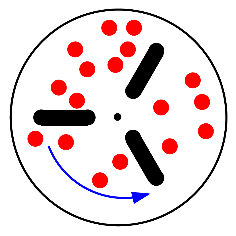
Figure 1. Horizontal cross-section of vertical centrifuge with a three-blade impeller.

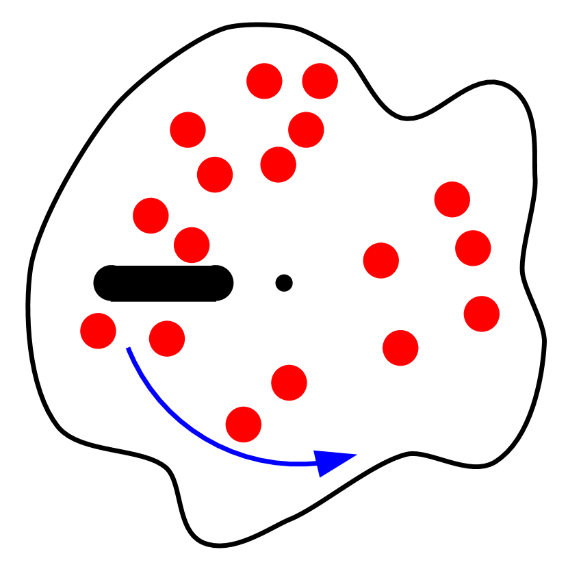
Figure 2. Horizontal cross-section of a rotating drum. The rotating walls include the outside boundary of the domain and an internal impeller.

It turns out that the dynamical system defined above has a conserved quantity and, as a consequence, there is no Fermi acceleration in this case. We will now present a more formal definition of the system and the conserved quantity.

Let $H$ be the two-dimensional subspace of $\mathds{R}^{d}$ spanned by the first two basis vectors. Consider a bounded $d$-dimensional domain with smooth boundary rotating with the constant angular velocity $\omega>0$ in $H$ about the origin. Let $P_{H}$ denote the projection on $H$ and let $\mathcal{R}(\theta)$ denote the rotation by angle $\theta$ in $H$. Set $L=\mathcal{R}(\pi/2)\circ P_{H}$. Suppose that the rotating drum $D$ holds $n$ balls, for some finite $n\geq 1$. Let $F$ be the moving frame of reference rotating with the centrifuge. In other words, the drum $D$ is static in $F$. For the $k$-th molecule, let $m_{k}$ be its mass, $v_{k}(t)\in\mathds{R}^{d}$ its velocity at time $t$, $v^{F}_{k}(t)\in\mathds{R}^{d}$ its velocity in $F$ at time $t$, $x_{k}(t)\in\mathds{R}^{d}$ its center at time $t$, $x_{k}^{F}(t)\in\mathds{R}^{d}$ its center in $F$ at time $t$, $x^{H}_{k}(t)\in H$ the projection of its center on $H$ at time $t$, and $x^{F,H}_{k}(t)\in H$ the projection of its center on $H$ in $F$ at time $t$. Note that $x^{H}_{k}(t)=P_{H}(x_{k}(t))$, $x^{F,H}_{k}(t)=P_{H}(x^{F}(t))$, $x_{k}^{F}(t)=\mathcal{R}(-\omega t)(x_{k}(t))$, $\|x^{F,H}_{k}(t)\|=\|x^{H}_{k}(t)\|$. The velocities are related by

(1.1) $$\mathcal{R}(\omega t)(v_{k}^{F}(t))=v_{k}(t)-\omega L(x_{k}(t))$$

(see Section 5.2). If $d=3$, the angular velocity is typically represented as the vector $\bm{\omega}:=\omega\bm{e_{3}}$ and then $\omega L(x_{k}(t))=\bm{\omega}\times x_{k}(t)$. Let

$$E^{F,K}(t) =\sum_{k=1}^{n}m_{k}\|v_{k}^{F}(t)\|^{2}/2,$$

(1.2) $$E^{F,P}(t) =-\sum_{k=1}^{n}m_{k}\omega^{2}\|x^{H}_{k}(t)\|^{2}/2,$$

$$E^{F}(t) =E^{F,K}(t)+E^{F,P}(t).$$

We will show in Propositions 5.4 and 2.1 that the quantity $E^{F}(t)$ is conserved, not only between collisions but also at collisions of balls or of a ball and a wall. Thus $E^{F}:=E^{F}(t)=E^{F}(0)$ for all $t\geq 0$. This can be interpreted as the conservation of energy in the rotating (non-inertial) frame of reference $F$. The sum of the “kinetic energy” $E^{F,K}(t)$ and “potential energy” $E^{F,P}(t)$, i.e., $E^{F}=E^{F,K}(t)+E^{F,P}(t)$, remains constant. The potential energy $E^{F,P}(t)$ is associated with the centrifugal force. There is no contribution from the Coriolis force. The usual kinetic energy in the inertial frame is of course preserved between collisions, since the balls are free, and at collisions of two balls, since these collisions are assumed elastic. But, as noted above, it is not preserved at collisions of a ball and a wall.

We will now sketch an argument that there is no Fermi acceleration, based on the conservation of $E^{F}$. Since the drum is represented by a bounded domain $D$ and the angular velocity $\omega$ is fixed, all quantities in the formula $-\sum_{k=1}^{n}m_{k}\omega^{2}\|x^{H}_{k}(t)\|^{2}/2$ stay bounded and, therefore, the potential energy $E^{F,P}(t)$ stays bounded. This and the fact that the energy $E^{F}$ is constant imply that the kinetic energy $E^{F,K}(t)$ must remain bounded. Again since the domain $D$ is bounded and $\omega$ is fixed, the difference $\|\mathcal{R}(\omega t)(v_{k}^{F}(t))-v_{k}(t)\|=\|\omega L(x_{k}(t))\|$ stays bounded. Thus the difference between $E^{F,K}(t)$ and the total energy in the inertial frame of reference $E^{K}(t):=\sum_{k=1}^{n}m_{k}\|v_{k}(t)\|^{2}/2$ remains bounded and, therefore, $E^{K}(t)$ remains bounded. Hence, there is no Fermi acceleration.

Next we describe an invariant measure for this model, a special case of the microcanonical ensemble (see [35, Sect. 1.2]). There are typically many invariant measures for the system defined above but the measure we will present is unique for some probabilistic systems defined later.

For $E^{F}\in\mathds{R}$, we will give a formula for an invariant measure on the level set

$$\mathcal{S}_{E^{F}}=\Big{\{}\left(x_{1}^{F},x_{2}^{F},\dots,x_{n}^{F},v_{1}^{F},v_{2}^{F},\dots,v_{n}^{F}\right):\sum_{k=1}^{n}m_{k}\|v_{k}^{F}\|^{2}/2-\sum_{k=1}^{n}m_{k}\omega^{2}\|x^{F,H}_{k}\|^{2}/2=E^{F}\Big{\}}$$

of the conserved function in the space of

$$\left(x_{1}^{F},x_{2}^{F},\dots,x_{n}^{F},v_{1}^{F},v_{2}^{F},\dots,v_{n}^{F}\right),$$

not $\left(x_{1},x_{2},\dots,x_{n},v_{1},v_{2},\dots,v_{n}\right)$. Since the balls have positive radii, the vector of centers $\left(x_{1}^{F},x_{2}^{F},\dots,x_{n}^{F}\right)$ is required to lie in the closed subset $\mathcal{D}$ of $D^{n}$ defined by the conditions that the interiors of the balls are contained in $D$ and do not overlap. Set $\mathcal{S}_{E^{F},\mathcal{D}}=\left\{\left(x_{1}^{F},x_{2}^{F},\dots,x_{n}^{F},v_{1}^{F},v_{2}^{F},\dots,v_{n}^{F}\right)\in\mathcal{S}_{E^{F}}:\left(x_{1}^{F},x_{2}^{F},\dots,x_{n}^{F}\right)\in\mathcal{D}\right\}$ and denote by $\mathcal{S}_{E^{F}}^{0}$, $\mathcal{S}_{E^{F},\mathcal{D}}^{0}$ the subsets of $\mathcal{S}_{E^{F}}$, $\mathcal{S}_{E^{F},\mathcal{D}}$, resp., for which $\left(v_{1}^{F},v_{2}^{F},\dots,v_{n}^{F}\right)\neq 0$; equivalently for which $E^{F}+\sum_{k=1}^{n}m_{k}\omega^{2}\|x^{F,H}_{k}\|^{2}/2>0$. Consider the bijection $\overline{\Phi}:\mathcal{S}^{0}_{E^{F},\mathcal{D}}\rightarrow\mathcal{D}\times S^{nd-1}$ given by

$$\overline{\Phi}\left(x_{1}^{F},x_{2}^{F},\dots,x_{n}^{F},v_{1}^{F},v_{2}^{F},\dots,v_{n}^{F}\right)=\left(x_{1}^{F},x_{2}^{F},\dots,x_{n}^{F},\overline{v}_{1}^{F},\overline{v}_{2}^{F},\dots,\overline{v}_{n}^{F}\right),$$

where $S^{nd-1}$ denotes the Euclidean unit sphere in $\mathds{R}^{nd}$ and

(1.3) $$\overline{v}_{k}^{F}=\frac{\sqrt{m_{k}}v_{k}^{F}}{\left(\sum_{k=1}^{n}m_{k}\|v_{k}^{F}\|^{2}\right)^{1/2}}.$$

On $\mathcal{S}^{0}_{E^{F},\mathcal{D}}$, the invariant measure can be written as

(1.4) $$f\left(x_{1}^{F},x_{2}^{F},\dots,x_{n}^{F}\right)\overline{\Phi}^{*}\left(d\sigma_{1}\left(\overline{v}_{1}^{F},\overline{v}_{2}^{F},\dots,\overline{v}_{n}^{F}\right)\,d\lambda\left(x_{1}^{F},x_{2}^{F},\dots,x_{n}^{F}\right)\right).$$

Here $d\sigma_{1}$ denotes the usual measure on the unit sphere $S^{nd-1}$, $d\lambda$ denotes Lebesgue measure on $\mathds{R}^{nd}$, $\overline{\Phi}^{*}\left(d\sigma_{1}\left(\overline{v}_{1}^{F},\overline{v}_{2}^{F},\dots,\overline{v}_{n}^{F}\right)\,d\lambda\left(x_{1}^{F},x_{2}^{F},\dots,x_{n}^{F}\right)\right)$ denotes the pullback of the product measure, and the density function $f$ is given by

(1.5) $$f\left(x_{1}^{F},x_{2}^{F},\dots,x_{n}^{F}\right)=\left(E^{F}+\sum_{k=1}^{n}m_{k}\omega^{2}\|x^{F,H}_{k}\|^{2}/2\right)^{nd/2-1}.$$

In particular, given $E^{F,P}$ (equivalently, given $E^{F,K}$, since $E^{F}$ is fixed), the kinetic energy of the system in the frame $F$ is equidistributed on the sphere, i.e., the vector

(1.6) $$\left(\sqrt{\frac{m_{1}}{2}}v_{1}^{F},\sqrt{\frac{m_{2}}{2}}v_{2}^{F},\dots,\sqrt{\frac{m_{n}}{2}}v_{n}^{F}\right)$$

is uniformly distributed on the $(nd-1)$-dimensional sphere centered at 0, with radius $\left(E^{F,K}\right)^{1/2}$.

1.2. Rotating drum with Lambertian reflections

Our next model is concerned with a rotating drum with a rough surface. On the mathematical side, this means that the walls $\partial D$ are smooth but reflections are not necessarily specular (i.e., the angle of reflection is not necessarily equal to the angle of incidence). We will consider a special class of random reflections. There are two sources of inspiration for this model. First, as we have already mentioned, gas centrifuges used for separation of uranium isotopes have cylindrical rotors. The surface of the rotor has to be rough or otherwise the molecules of gas would not have a tendency to rotate. The second reason for introducing random reflections is that the microcanonical ensemble is not the only invariant measure for the dynamical system described in Section 1.1. Fig. 3 shows a trivial invariant measure represented by a closed orbit of a single particle. The invariant measure is unique if the reflections from the walls are random; more precisely, it is unique for some random reflection laws.

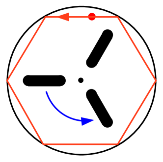
Figure 3. An invariant measure is represented by the closed orbit of a single particle.

Random reflections can be rigorously defined for hard balls of any size but on the physics side, only reflections of small balls from a rough surface can be expected to be random according to the definitions given below.

We will limit our model to random reflections which are natural in two ways: (i) the microcanonical ensemble is an invariant measure for the model with random reflections and (ii) the random reflections are the limit of deterministic reflections from rough (fractal) surfaces, assuming that the size of small crystals forming the rough surface goes to zero. Reflection laws with these properties have been studied in [3, 17, 29, 30, 31]. We will recall the characterization of such laws in Section 3.1. We will also state and prove an immediate corollary of that result, saying that if the random angle of reflection does not depend on the angle of incidence then the reflection law must be Lambertian, also known as the Knudsen law, defined as follows. Let $S^{d-1}$ be the unit sphere in $\mathds{R}^{d}$, let $S^{d-1}_{+}=\{(x_{1},x_{2},\dots,x_{d})\in S^{d-1}:x_{d}>0\}$, and ${\bf n}=(0,0,\dots,0,1)$. We say that the probability measure $\nu_{d}$ on $S^{d-1}_{+}$ is Lambertian if its density with respect to usual surface measure is

(1.7) $$f(v)=b_{d}\langle v,{\bf n}\rangle,$$

where $b_{d}>0$ is the normalizing constant.

Although Lambert’s work [24] precedes that of Knudsen [23] by more than one and a half centuries, it is appropriate to use Knudsen’s name in our context because he applied his model to gases, while Lambert was concerned with reflections of light.

We will consider a cylindrical drum rotating about its axis and a single pointlike particle reflecting from its surface. We will assume that the reflections are Lambertian in the frame of reference $F$. We will derive a formula for the expected value of the duration of the free flight between reflections from the cylindrical walls. We will show that the asymptotic winding number about the axis of rotation for the particle is equal to the angular velocity of the cylindrical rotor.

1.3. Rotating drum with gravitation and Lambertian reflections

The last model that we consider includes Lambertian reflections and gravitation. It is inspired by a bingo machine (see Fig. 4). In this case, we consider a pointlike particle reflecting from an infinitely heavy circular wall of a 2-dimensional drum with smooth or rough surface, and subject to gravitational force acting in the plane of rotation. We argue that there is Fermi acceleration in this model. The precise statement is given in Section 4. We note here that the mathematical heart of the argument is concerned with a simplified model in which two points are fixed on the wall in the inertial frame of reference (so that they do not move with the wall; see Fig. 5). We study a trajectory whose reflections alternate between the two fixed points. The segments of the trajectory become closer and closer to line segments and the energy of the reflecting particle goes to infinity. This simplified model is the basis of somewhat more realistic theorems.

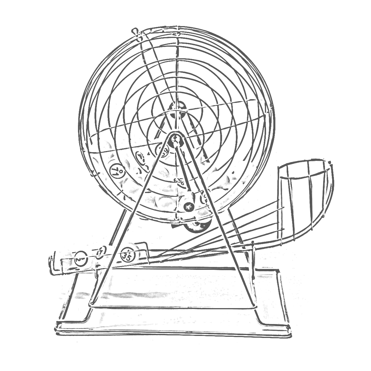
Figure 4. Bingo machine.

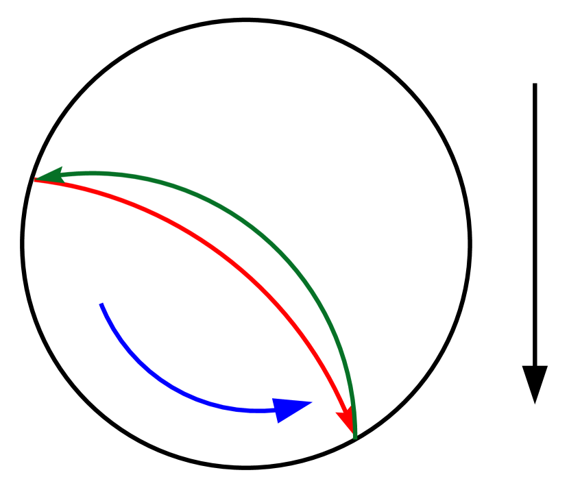
Figure 5. Rotating drum with gravitation and pseudo-Lambertian reflections. The black arrow represents gravity. The blue arrow represents angular velocity. The red and green paths represent two (of infinitely many) parabolic segments of a trajectory hitting two points fixed in the inertial frame of reference.

1.4. Literature review

Our paper involves Fermi acceleration, billiards with gravity, billiards with rotation, and Lambertian reflections, so we briefly review the literature on these topics.

There is vast literature on Fermi acceleration. We point out a recent addition [38], concerned with rectangular billiards with moving slits, because it is both interesting and contains an extensive literature review. See [15, 22, 26, 32] for surveys of Fermi acceleration.

Billiards with gravitation or other forces or potentials were considered in [13, 14, 16, 34].

Billiards models incorporating time-dependent boundaries, rotation, breathing walls or similar effects originated in the papers [21, 36] and were more recently analyzed in [4, 13, 16, 28, 33].

The relationship between rough billiard boundaries and random reflections (including Lambertian reflections; equivalently Knudsen law) was studied in [3, 10, 11, 12, 17, 18, 19, 20, 29, 30, 31].

2. Rotating drum with arbitrary shape and specular reflections

In this section we consider a rotating drum represented by a bounded domain $D\subset\mathds{R}^{d}$, for some $d\geq 2$, with smooth boundary, rotating with a fixed angular velocity $\omega>0$. The rotation applies only to a 2-dimensional plane $H$. All other coordinates of points in $D$ remain constant. We suppose that the drum $D$ holds $n$ hard (non-intersecting) balls for some finite $n\geq 1$. We will write $m_{k}>0$ for the mass of the $k$-th ball, $v_{k}(t)\in\mathds{R}^{d}$ will stand for its velocity at time $t$, and $x_{k}(t)\in\mathds{R}^{d}$ will be its center at time $t$.

To avoid uninteresting technical complications, we will assume that the curvature of $\partial D$ is small relative to the radii of the balls. More precisely, let $r_{\max}$ be the maximum of the ball radii. We will assume that for every point $y\in\partial D$, there is exactly one open ball of radius $r_{\max}$ contained in $D$ whose boundary is tangent to $\partial D$ at $y$, and the closure of this ball touches $\partial D$ only at $y$.

In this section we will assume that $\partial D$ and the surfaces of the balls are perfectly smooth so that their collisions do not involve friction and, therefore, they do not change the angular velocities of the balls. Hence, we can and will assume that the balls do not rotate.

We will assume that there are no simultaneous collisions of more than two balls (see [6] for a precise formulation). Unlike for collisions of two balls, in a simultaneous collision of more than two balls the evolution of the system is not uniquely determined by conservation of energy, momentum and angular momentum (see, for example [37]). In view of this assumption and that of the previous paragraph, for the evolution of the system to be uniquely defined at a collision, it is enough to assume conservation of energy and momentum. We will also assume that when a ball collides with the wall $\partial D$, it does not collide with another ball at the same time. The law of specular reflection in the rotating frame then determines the evolution at collisions involving the wall. The wall $\partial D$ will be assumed to be infinitely heavy so that we will exclude it from the energy and momentum balances.

Let $F$ be the non-inertial frame of reference which makes $D$ static. For the $k$-th particle, let $v^{F}_{k}(t)\in\mathds{R}^{d}$ be its velocity in $F$ at time $t$, given by (1.1), and $x^{H}_{k}(t)\in H$ be the projection of its center on $H$ at time $t$. Recall the definitions (1.1) of the energy quantities in $F$.

Recall from Section 1.1 that $L=\mathcal{R}(\pi/2)\circ P_{H}$, and note that for all $x$,

(2.1) $$\langle x,L(x)\rangle=\langle x-P_{H}(x),\mathcal{R}(\pi/2)\circ P_{H}(x)\rangle+\langle P_{H}(x),\mathcal{R}(\pi/2)\circ P_{H}(x)\rangle=0+0=0.$$

Proposition 2.1.

The energy $E^{F}(t)$ is a conserved quantity, i.e., it depends only on the initial conditions; it does not depend on time $t$.

Proof.

It follows from Proposition 5.4 that $E^{F}(t)$ does not depend on $t$ between collisions. We will next argue that $E^{F}(t)$ does not change its value at collision times.

The positions $x_{k}(t)$ are continuous across a collision time while the velocities $v_{k}(t)$ may have a jump discontinuity. The quantity $E^{F,P}(t)$ is therefore continuous so it suffices to show that $E^{F,K}(t)$ is continuous.

Suppose that balls $j$ and $k$ collide at time $s>0$. We denote $v_{j}^{\pm}=\lim_{t\to s^{\pm}}v_{j}(t)$ and similarly for $v_{k}^{\pm}$, $v_{j}^{F,\pm}$, and $v_{k}^{F,\pm}$. Since the collision is elastic, momentum and energy are conserved across the collision, so

$$m_{j}v_{j}^{+}+m_{k}v_{k}^{+} =m_{j}v_{j}^{-}+m_{k}v_{k}^{-}$$

$$m_{j}\|v_{j}^{+}\|^{2}+m_{k}\|v_{k}^{+}\|^{2} =m_{j}\|v_{j}^{-}\|^{2}+m_{k}\|v_{k}^{-}\|^{2}.$$

Using (1.1), we have

$$m_{j}\|v_{j}^{F}(t)\|^{2}+m_{j}\|v_{k}^{F}(t)\|^{2} =m_{j}\|v_{j}(t)-\omega L(x_{j}(t))\|^{2}+m_{k}\|v_{k}(t)-\omega L(x_{k}(t))\|^{2}$$

$$=m_{j}\|v_{j}(t)\|^{2}+m_{k}\|v_{k}(t)\|^{2}$$

$$\quad+m_{j}\omega^{2}\|L(x_{j}(t))\|^{2}+m_{k}\omega^{2}\|L(x_{k}(t))\|^{2}$$

$$\quad-2m_{j}\omega\langle v_{j}(t),L(x_{j}(t))\rangle-2m_{k}\omega\langle v_{k}(t),L(x_{k}(t))\rangle.$$

The first line after the last equality is continuous across the collision by conservation of energy in the inertial frame. The second line after the last equality is continuous since the quantities which appear in it are continuous. So it suffices to show that the last line is continuous across the collision. Denote $x_{j}(s)$, $x_{k}(s)$ simply by $x_{j}$, $x_{k}$. Using conservation of momemtum across the collision in the inertial frame, we have

$$\lim_{t\to s^{+}} \big{[}m_{j}\langle v_{j}(t),L(x_{j}(t))\rangle+m_{k}\langle v_{k}(t),L(x_{k}(t))\rangle\big{]}$$

$$=m_{j}\langle v_{j}^{+},L(x_{j})\rangle+m_{k}\langle v_{k}^{+},L(x_{k})\rangle$$

$$=m_{j}\langle v_{j}^{+},L(x_{j})\rangle+m_{k}\langle v_{k}^{+},L(x_{j})\rangle+m_{k}\langle v_{k}^{+},L(x_{k}-x_{j})\rangle$$

$$=\langle m_{j}v_{j}^{+}+m_{k}v_{k}^{+},L(x_{j})\rangle+m_{k}\langle v_{k}^{+},L(x_{k}-x_{j})\rangle$$

$$=\langle m_{j}v_{j}^{-}+m_{k}v_{k}^{-},L(x_{j})\rangle+m_{k}\langle v_{k}^{+},L(x_{k}-x_{j})\rangle$$

$$=m_{j}\langle v_{j}^{-},L(x_{j})\rangle+m_{k}\langle v_{k}^{-},L(x_{k})\rangle+m_{k}\langle v_{k}^{-},L(x_{j}-x_{k})\rangle+m_{k}\langle v_{k}^{+},L(x_{k}-x_{j})\rangle$$

$$=\lim_{t\to s^{-}}\big{[}m_{j}\langle v_{j}(t),L(x_{j}(t))\rangle+m_{k}\langle v_{k}(t),L(x_{k}(t))\rangle\big{]}+m_{k}\langle v_{k}^{+}-v_{k}^{-},L(x_{k}-x_{j})\rangle.$$

In an elastic collision of two balls, the component of velocity of each ball orthogonal to the line connecting the centers at the time of collision is continuous; it is only the component of velocity in the direction of the line of centers which reflects. So $v_{k}^{+}-v_{k}^{-}$ is a multiple of $x_{k}-x_{j}$. Since $\langle x,L(x)\rangle=0$ for all $x$ (see (2.1)), it follows the second term on the last line vanishes so that $E^{F,K}(t)$ is continuous across a collision time of two balls.

It is clear that $E^{F}(t)$ is continuous at the time of a collision between a ball and the wall $\partial D$ since the ball reflects according to the law of specular reflection in the frame $F$, so that $\|v^{F}(t)\|$ is preserved. We conclude that $E^{F}(t)$ is in fact a constant $E^{F}$. ∎

Proposition 2.2.

Let

$$R=\sup_{x\in D}\|x^{H}\|,\quad M=\sum_{k=1}^{n}m_{k},\quad E^{K}(t)=\sum_{k=1}^{n}m_{k}\|v_{k}(t)\|^{2}/2,$$

and let $E^{F}:=E^{F}(0)=E^{F}(t)$. For all $t>0$,

$$E^{K}(t)\leq 2E^{F}+2M\omega^{2}R^{2}.$$

In particular, since $E^{F}$ is constant, there is no Fermi acceleration.

Proof.

For all $t$,

(2.2) $$0\leq\left|E^{F,P}(t)\right|=\sum_{k=1}^{n}m_{k}\omega^{2}\|x^{H}_{k}(t)\|^{2}/2\leq M\omega^{2}R^{2}/2.$$

We have $\|\mathcal{R}(\omega t)(v_{k}^{F}(t))-v_{k}(t)\|=\omega\|L(x_{k}(t))\|\leq\omega R$, so

$$\|v_{k}(t)\|^{2} \leq 2\|v_{k}^{F}(t)\|^{2}+2\|\mathcal{R}(\omega t)(v_{k}^{F}(t))-v_{k}(t)\|^{2}\leq 2\|v_{k}^{F}(t)\|^{2}+2\omega^{2}R^{2}.$$

This and (2.2) imply that for any $t>0$,

$$E^{K}(t) =\sum_{k=1}^{n}\frac{m_{k}}{2}\|v_{k}(t)\|^{2}\leq\sum_{k=1}^{n}m_{k}\left(\|v_{k}^{F}(t)\|^{2}+\omega^{2}R^{2}\right)=2E^{F,K}(t)+M\omega^{2}R^{2}$$

$$=2(E^{F}-E^{F,P}(t))+M\omega^{2}R^{2}\leq 2E^{F}+2M\omega^{2}R^{2}.$$

∎

The next proposition concerns the invariant measure. Proposition 5.4 describes the invariant measure for the dynamical system consisting of noninteracting point particles free to roam in the whole Euclidean space. Our vector of centers $\left(x_{1}^{F},x_{2}^{F},\dots,x_{n}^{F}\right)$ is constrained to lie in $\mathcal{D}$, which has boundaries corresponding to collisions of the balls or of balls and the wall $\partial D$. Recall the level set $\mathcal{S}_{E^{F}}$ and its subsets $\mathcal{S}_{E^{F},\mathcal{D}}$ and $\mathcal{S}^{0}_{E^{F},\mathcal{D}}$ defined in the introduction.

Proposition 2.3.

Fix energy $E^{F}$ such that $\mathcal{S}^{0}_{E^{F},\mathcal{D}}\neq\emptyset$. The measure defined in (1.4) and (1.5) is the restriction to $\mathcal{S}^{0}_{E^{F},\mathcal{D}}$ of an invariant measure on $\mathcal{S}_{E^{F},\mathcal{D}}$.

Proof.

The invariant measure on $\mathcal{S}_{E^{F}}$ in the statement of Proposition 5.4 restricts to a measure on $\mathcal{S}_{E^{F},\mathcal{D}}\subset\mathcal{S}_{E^{F}}$ (making the obvious adjustment since the discussion in Section 5 is formulated in terms of momenta instead of velocities), which is invariant for $\left(x_{1}^{F},\dots,x_{n}^{F}\right)\notin\partial\mathcal{D}$, and whose restriction to $\mathcal{S}^{0}_{E^{F},\mathcal{D}}$ has the form (1.4), (1.5). It remains to analyze the collisions.

Recall that we are not considering simultaneous collisions of more than two balls nor collisions in which a ball collides with $\partial D$ at the same time that it collides with another ball. It is known that the set of initial conditions giving rise to simultaneous collisions of more than two balls has measure zero ([2]). We believe that the arguments of that paper apply also to simultaneous collisions of $\partial D$ and more than one ball.

At each point of $\partial\mathcal{D}$ corresponding to a collision of two balls or of a ball and $\partial D$, there is a collision map from the space of vectors of incoming velocities to that of outgoing velocities. It suffices to show that this map on velocities preserves the measure $d\sigma_{1}\left(\overline{v}_{1}^{F},\overline{v}_{2}^{F},\ldots,\overline{v}_{n}^{F}\right)$ appearing in (1.4).

Suppose that balls $j$ and $k$ collide at time $s>0$. The components of $v_{j}(t)$ and $v_{k}(t)$ orthogonal to the line connecting the locations $x_{j}(s)$ and $x_{k}(s)$ of the centers at time $s$ are continuous; only the components parallel to this line can jump. Set $\bm{e^{\|}}=\frac{x_{k}(s)-x_{j}(s)}{\|x_{k}(s)-x_{j}(s)\|}$ and

$$v_{j}^{\|\pm}=\lim_{t\to s^{\pm}}\left\langle v_{j}(t),\bm{e^{\|}}\right\rangle,\qquad v_{k}^{\|\pm}=\lim_{t\to s^{\pm}}\left\langle v_{k}(t),\bm{e^{\|}}\right\rangle.$$

A collision occurs only if $v_{j}^{\|-}>v_{k}^{\|-}$. This condition defines the space of incoming velocities. The space of outgoing velocities is defined by the complementary condition $v_{j}^{\|+}<v_{k}^{\|+}$. For the frame $F$ we similarly set

$$v_{j}^{F,\|\pm}=\lim_{t\to s^{\pm}}\left\langle\mathcal{R}(\omega t)v_{j}^{F}(t),\bm{e^{\|}}\right\rangle,\qquad v_{k}^{F,\|\pm}=\lim_{t\to s^{\pm}}\left\langle\mathcal{R}(\omega t)v_{k}^{F}(t),\bm{e^{\|}}\right\rangle.$$

In light of (1.1), we have

(2.3) $$v_{j}^{F,\|\pm}=v_{j}^{\|\pm}-\omega\left\langle L(x_{j}(s)),\bm{e^{\|}}\right\rangle$$

and similarly for $v_{k}^{F,\|\pm}$. On the right-hand side, the term $-\omega\left\langle L(x_{j}(s)),\bm{e^{\|}}\right\rangle$ is the same for both equations corresponding to $\pm$. Since $x_{j}(s)-x_{k}(s)$ is a multiple of $\bm{e^{\|}}$ and $\langle L(x),x\rangle=0$ for all $x$, the incoming and outgoing conditions are equivalent to $v_{j}^{F,\|-}>v_{k}^{F,\|-}$ and $v_{j}^{F,\|+}<v_{k}^{F,\|+}$.

Standard formulas for the transformation of velocities in a totally elastic reflection of balls in one dimension can be written in the following form

$$\begin{pmatrix}\sqrt{m_{j}}v_{j}^{\|+}\\ \\ \sqrt{m_{k}}v_{k}^{\|+}\end{pmatrix}=\begin{pmatrix}\displaystyle\frac{2\sqrt{m_{j}m_{k}}}{m_{j}+m_{k}}&\displaystyle\frac{m_{j}-m_{k}}{m_{j}+m_{k}}\\ \\ \displaystyle\frac{m_{k}-m_{j}}{m_{j}+m_{k}}&\displaystyle\frac{2\sqrt{m_{j}m_{k}}}{m_{j}+m_{k}}\end{pmatrix}\begin{pmatrix}\sqrt{m_{k}}v_{k}^{\|-}\\ \\ \sqrt{m_{j}}v_{j}^{\|-}\end{pmatrix}.$$

We claim that the same relation holds with $v_{j}^{\|+}$, $v_{k}^{\|+}$, $v_{j}^{\|-}$, $v_{k}^{\|-}$ replaced by $v_{j}^{F,\|+}$, $v_{k}^{F,\|+}$, $v_{j}^{F,\|-}$, $v_{k}^{F,\|-}$, i.e.

(2.4) $$\begin{pmatrix}\sqrt{m_{j}}v_{j}^{F,\|+}\\ \\ \sqrt{m_{k}}v_{k}^{F,\|+}\end{pmatrix}=\begin{pmatrix}\displaystyle\frac{2\sqrt{m_{j}m_{k}}}{m_{j}+m_{k}}&\displaystyle\frac{m_{j}-m_{k}}{m_{j}+m_{k}}\\ \\ \displaystyle\frac{m_{k}-m_{j}}{m_{j}+m_{k}}&\displaystyle\frac{2\sqrt{m_{j}m_{k}}}{m_{j}+m_{k}}\end{pmatrix}\begin{pmatrix}\sqrt{m_{k}}v_{k}^{F,\|-}\\ \\ \sqrt{m_{j}}v_{j}^{F,\|-}\end{pmatrix}.$$

According to (2.3), this is equivalent to the identity

$$\begin{pmatrix}\sqrt{m_{j}}\left\langle L(x_{j}(s),\bm{e^{\|}}\right\rangle\\ \\ \sqrt{m_{k}}\left\langle L(x_{k}(s),\bm{e^{\|}}\right\rangle\end{pmatrix}=\begin{pmatrix}\displaystyle\frac{2\sqrt{m_{j}m_{k}}}{m_{j}+m_{k}}&\displaystyle\frac{m_{j}-m_{k}}{m_{j}+m_{k}}\\ \\ \displaystyle\frac{m_{k}-m_{j}}{m_{j}+m_{k}}&\displaystyle\frac{2\sqrt{m_{j}m_{k}}}{m_{j}+m_{k}}\end{pmatrix}\begin{pmatrix}\sqrt{m_{k}}\left\langle L(x_{k}(s),\bm{e^{\|}}\right\rangle\\ \\ \sqrt{m_{j}}\left\langle L(x_{j}(s),\bm{e^{\|}}\right\rangle\end{pmatrix}.$$

A little computation shows that both components of this vector equation reduce to $\left\langle L(x_{j}(s)-x_{k}(s)),\bm{e^{\|}}\right\rangle=0$. As above, this holds since $x_{j}(s)-x_{k}(s)$ is a multiple of $\bm{e^{\|}}$ and $\langle L(x),x\rangle=0$ for all $x$. Thus (2.4) is verified.

Since $m_{j},m_{k}>0$ and

$$\left(\frac{2\sqrt{m_{j}m_{k}}}{m_{j}+m_{k}}\right)^{2}+\left(\frac{m_{j}-m_{k}}{m_{j}+m_{k}}\right)^{2}=1,$$

there is a unique $\alpha\in(-\pi/2,\pi/2)$ such that

$$\cos\alpha=\frac{2\sqrt{m_{j}m_{k}}}{m_{j}+m_{k}},\qquad\sin\alpha=\frac{m_{k}-m_{j}}{m_{j}+m_{k}}.$$

Hence we can write

(2.5) $$\begin{pmatrix}\displaystyle\sqrt{m_{j}}v_{j}^{F,\|+}\\ \displaystyle\sqrt{m_{k}}v_{k}^{F,\|+}\end{pmatrix}=\begin{pmatrix}\cos\alpha&-\sin\alpha\\ \sin\alpha&\cos\alpha\end{pmatrix}\begin{pmatrix}\displaystyle\sqrt{m_{k}}v_{k}^{F,\|-}\\ \displaystyle\sqrt{m_{j}}v_{j}^{F,\|-}\end{pmatrix}.$$

The incoming condition $v_{j}^{F,\|-}>v_{k}^{F,\|-}$ can be rewritten as

(2.6) $$\sqrt{m_{j}}v_{j}^{F,\|-}>\sqrt{\frac{m_{j}}{m_{k}}}\sqrt{m_{k}}v_{k}^{F,\|-}.$$

Straightforward calculations show that the map

$$\begin{pmatrix}u_{1}^{-}\\ u_{2}^{-}\end{pmatrix}\mapsto\begin{pmatrix}u_{1}^{+}\\ u_{2}^{+}\end{pmatrix}=\begin{pmatrix}\cos\alpha&-\sin\alpha\\ \sin\alpha&\cos\alpha\end{pmatrix}\begin{pmatrix}u_{2}^{-}\\ u_{1}^{-}\end{pmatrix}$$

is a bijection between the incoming half-plane $u_{1}^{-}>\sqrt{\frac{m_{j}}{m_{k}}}u_{2}^{-}$ and the outgoing half-plane $u_{1}^{+}<\sqrt{\frac{m_{j}}{m_{k}}}u_{2}^{+}$.

The transformation in (2.5) is the composition of the symmetry

$$\left(\sqrt{m_{j}}v_{j}^{F,\|-},\sqrt{m_{k}}v_{k}^{F,\|-}\right)\to\left(\sqrt{m_{k}}v_{k}^{F,\|-},\sqrt{m_{j}}v_{j}^{F,\|-}\right)$$

and rotation by the angle $\alpha$. Since the collision map leaves constant the velocity components orthogonal to $\bm{e^{\|}}$ and the velocities of the noncolliding balls, it is an orthogonal transformation in the space of $\left(\overline{v}_{1}^{F},\overline{v}_{2}^{F},\ldots,\overline{v}_{n}^{F}\right)$ given by (1.3), so certainly it maps the measure $d\sigma_{1}\left(\overline{v}_{1}^{F},\overline{v}_{2}^{F},\ldots,\overline{v}_{n}^{F}\right)$ on the incoming half-sphere to the same measure on the outgoing half-sphere. This completes the proof in the case of the collision of two balls.

The collision of a ball with the wall of the rotating drum is simpler. If the $j$-th ball collides with $\partial D$ at time $s$ and $\bm{\nu}$ denotes the outward-pointing normal at the point of contact, the incoming velocities are those for which $\langle v_{j}^{F}(s),\bm{\nu}\rangle>0$ and the outgoing velocities are those for which $\langle v_{j}^{F}(s),\bm{\nu}\rangle<0$. The collision map just reflects $v_{j}^{F}(s)$ across the tangent plane to $\partial D$ and leaves all other velocities unchanged. This map clearly preserves the measure $d\sigma_{1}\left(\overline{v}_{1}^{F},\overline{v}_{2}^{F},\ldots,\overline{v}_{n}^{F}\right)$. ∎

3. A pointlike particle in rotating drum

In this section, we will focus on the case of a single pointlike particle in a rotating drum. This model is inspired by “Knudsen gas,” i.e., gas diluted to the point that molecules typically do not collide on the length scale of the diameter of the drum; see [23].

3.1. Lambertian reflections as a model for a rough surface

In this subsection we will prove in Corollary 3.2 that the Knudsen reflection law (1.7) is the only random reflection distribution which can arise from classical specular reflections from a fractal surface consisting of small smooth crystals if we assume homogeneity and lack of memory, i.e., if we assume that the limiting distribution of the angle of reflection does not depend on the angle of incidence, and it is the same at all boundary points.

Corollary 3.2 follows easily from results in [3, 17, 29, 30, 31], stated below as Propositions 3.1 and 3.3. The results in [3] rediscovered (independently) those in [30]; both articles were concerned with two-dimensional models. The full generality in an arbitrary number of dimensions was achieved in [29, 31]. Our presentation will combine [3, Thms. 2.2, 2.3], [17, Sect. 4] and [31, Thms. 4.4, 4.5]. For a very detailed and careful presentation of the billiards model in the plane see [9, Ch. 2]. For the multidimensional setup see [31]. We will be somewhat informal as the technical aspects of the model are tangential to our project.

Suppose that $M$ is a subset of the half-space $\{(x_{1},x_{2},\dots,x_{d})\in\mathds{R}^{d}:x_{d}\leq 0\}$ and its intersection with every ball (with finite radius) consists of a finite number of smooth surfaces. Informally, $M$ consists of very small mirrors (walls of billiard tables) that are supposed to model a macroscopically flat but rough reflecting surface.

Recall (1.7) and the definitions preceding it. Let $L_{*}=\{(x_{1},x_{2},\dots,x_{d})\in\mathds{R}^{d}:x_{d}=0\}$ and $B=L_{*}\times S^{d-1}_{+}$. Define a $\sigma$-finite measure $\Lambda(dx,dv)$ on $B$ as the product of Lebesgue measure on $L_{*}$ and $\nu_{d}$ on $S^{d-1}_{+}$.

We will consider a pointlike particle trajectory in $\mathds{R}^{d}$ starting on $L_{*}$. We will consider trajectories which are straight line segments between reflections and will assume that they reflect from surfaces comprising $M$ according to the rule of specular reflection, that is, the angle of incidence is equal to the angle of reflection, for every reflection.

Suppose that a trajectory starts from $x\in L_{*}$ in the direction $-v$, where $v\in S^{d-1}_{+}$, at time 0, reflects from surfaces of $M$ and returns to $y\in L_{*}$ at a time $t$, and $t>0$ is the smallest time with this property. Let $w\in S^{d-1}_{+}$ be the velocity of the particle at time $t$. This defines a mapping $K:B\to B$, given by $K(x,v)=(y,w)$. Clearly, $K$ depends on $M$.

It can be proved (see, e.g., [3, Prop. 2.1]) that under mild and natural assumptions, for $\Lambda$-almost all $(x,v)\in B$, a trajectory starting from $x$ with velocity $-v$, and reflecting from surfaces comprising $M$ will return to $L_{*}$ after a finite number of reflections.

We will write $\operatorname{\mathds{P}}(x,v;dy,dw)$ to denote a Markov transition kernel on $B$, that is, for fixed $(x,v)\in B$, $\operatorname{\mathds{P}}(x,v;dy,dw)$ is a probability measure on $B$. We assume that $\operatorname{\mathds{P}}$ satisfies the usual measurability conditions in all variables.

We will use $\delta_{x}(y)$ to denote Dirac’s delta function. Recall the transformation $K$ and let $\operatorname{\mathds{P}}_{K}$ be defined by $\operatorname{\mathds{P}}_{K}(x,v;dy,dw)=\delta_{K(x,v)}(y,w)dydw$. In other words, $\operatorname{\mathds{P}}_{K}$ represents a deterministic Markov kernel, with the atom at $K(x,v)$.

If $\mu_{n}$, $n\geq 1$, and $\mu_{\infty}$ are non-negative $\sigma$-finite measures on some measurable space $\Gamma$ then we will say that $\mu_{n}$ converge weakly to $\mu_{\infty}$ if there exists a sequence of sets $\Gamma_{j}$, $j\geq 1$, such that $\bigcup_{j\geq 1}\Gamma_{j}=\Gamma$, $\mu_{n}(\Gamma_{j})<\infty$, $\mu_{\infty}(\Gamma_{j})<\infty$ for all $n$ and $j$, and for every fixed $j$, the finite measures $\mu_{n}|_{\Gamma_{j}}$ converge weakly to $\mu_{\infty}|_{\Gamma_{j}}$.

Proposition 3.1.

Suppose that for some sequence of sets $M_{n}$, corresponding transformations $K_{n}$, and some Markov transition kernel $\operatorname{\mathds{P}}(x,v;dy,dw)$, we have

$$\Lambda(dx,dv)\operatorname{\mathds{P}}_{K_{n}}(x,v;dy,dw)\to\Lambda(dx,dv)\operatorname{\mathds{P}}(x,v;dy,dw)$$

in the sense of weak convergence on $B^{2}$ as $n\to\infty$. Then $\operatorname{\mathds{P}}$ is symmetric with respect to $\Lambda$ in the sense that for any smooth functions $f$ and $g$ on $B$ with compact support we have

$$\int_{B^{2}}f(y,w)\operatorname{\mathds{P}}(x,v;dy,dw)g(x,v)\Lambda(dx,dv)=\int_{B^{2}}g(y,w)\operatorname{\mathds{P}}(x,v;dy,dw)f(x,v)\Lambda(dx,dv).$$

In particular, $\Lambda$ is invariant in the sense that

(3.1) $$\int_{B^{2}}f(y,w)\operatorname{\mathds{P}}(x,v;dy,dw)\Lambda(dx,dv)=\int_{B}f(x,v)\Lambda(dx,dv).$$

Recall that $\delta_{x}(y)$ denotes Dirac’s delta function. Suppose that the probability kernel $\operatorname{\mathds{P}}$ in Proposition 3.1 satisfies $\operatorname{\mathds{P}}(x,v;dy,dw)=\delta_{x}(y)dy\widetilde{\operatorname{\mathds{P}}}(x,v;dw)$ for some $\widetilde{\operatorname{\mathds{P}}}$. Heuristically, this means that the trajectory starting at $x$ is instantaneously reflected from a mirror located infinitesimally close to $L_{*}$. Then (3.1) implies that for all smooth bounded functions $f$ on $S^{d-1}_{+}$, and almost all $x$,

(3.2) $$\int_{\left(S^{d-1}_{+}\right)^{2}}f(w)\widetilde{\operatorname{\mathds{P}}}(x,v;dw)\nu_{d}(dv)=\int_{S^{d-1}_{+}}f(v)\nu_{d}(dv).$$

If, in addition, we assume that $\widetilde{\operatorname{\mathds{P}}}(x,v;dw)=\widetilde{\operatorname{\mathds{P}}}(dw)$, i.e., $\widetilde{\operatorname{\mathds{P}}}(x,v;dw)$ does not depend on $x$ and $v$, then for all smooth bounded functions $f$ on $S^{d-1}_{+}$,

$$\int_{\left(S^{d-1}_{+}\right)^{2}}f(w)\widetilde{\operatorname{\mathds{P}}}(dw)\nu_{d}(dv)=\int_{S^{d-1}_{+}}f(v)\nu_{d}(dv),$$

and, therefore,

(3.3) $$\int_{S^{d-1}_{+}}f(w)\widetilde{\operatorname{\mathds{P}}}(dw)=\int_{S^{d-1}_{+}}f(v)\nu_{d}(dv).$$

Hence, $\widetilde{\operatorname{\mathds{P}}}(dw)=\nu_{d}(dw)$. We have just proved the following result.

Corollary 3.2.

Suppose that for some sequence of sets $M_{n}$, corresponding transformations $K_{n}$, and some $\widetilde{\operatorname{\mathds{P}}}(dw)$, we have

$$\Lambda(dx,dv)\operatorname{\mathds{P}}_{K_{n}}(x,v;dy,dw)\to\Lambda(dx,dv)\widetilde{\operatorname{\mathds{P}}}(dw)$$

in the sense of weak convergence on $B^{2}$ as $n\to\infty$. Then

(3.4) $$\widetilde{\operatorname{\mathds{P}}}(dw)=\nu_{d}(dw),\qquad w\in S^{d-1}_{+}.$$

Recall that a reflection law is called Lambertian or Knudsen if it is given by (1.7) (in particular, it does not depend on the angle of incidence). Hence, under the assumptions of Corollary 3.2, the limiting reflection law is Lambertian.

Proposition 3.3.

Suppose that $\operatorname{\mathds{P}}(x,v;dy,dw)=\delta_{x}(y)dy\widetilde{\operatorname{\mathds{P}}}(x,v;dw)$ where $\widetilde{\operatorname{\mathds{P}}}$ satisfies for smooth $f$ and $g$,

$$\int_{\left(S^{d-1}_{+}\right)^{2}}f(w)\widetilde{\operatorname{\mathds{P}}}(x,v;dw)g(v)\nu_{d}(dv)=\int_{\left(S^{d-1}_{+}\right)^{2}}g(w)\widetilde{\operatorname{\mathds{P}}}(x,v;dw)f(v)\nu_{d}(dv).$$

Then there exists a sequence of sets $M_{n}$ and corresponding transformations $K_{n}$ such that

$$\Lambda(dx,dv)\operatorname{\mathds{P}}_{K_{n}}(x,v;dy,dw)\to\Lambda(dx,dv)\operatorname{\mathds{P}}(x,v;dy,dw)$$

weakly on $B^{2}$ as $n\to\infty$. Moreover, $M_{n}$ can be chosen in such a way that $M_{n}\subset\{(x_{1},x_{2},\dots,x_{d}):-1/n<x_{d}\leq 0\}$.

Remark 3.4.

The proposition applies to $\widetilde{\operatorname{\mathds{P}}}$ in (3.4), so a dynamical system with Lambertian reflections is the limit of a sequence of systems with specular deterministic reflections.

We will later apply our results from Section 5 and Proposition 2.3 on the stationary distribution given in (1.4)-(1.5) to the approximating sets $M_{n}$. Since we prove these results for smooth boundaries, we point out that it is easy to see that the sets $M_{n}$ in Proposition 3.3 can be chosen to be smooth.

3.2. Pointlike particle in cylindrical drum

We will now compute the average flight time for a single particle in a rotating cylindrical drum in $\mathds{R}^{d}$, $d\geq 2$, with a rough surface, i.e., with the Knudsen reflection law.

Since we are dealing with a single particle in this section, we will drop the subscript from the notation introduced in Section 1.1 and we will write $x(t)$ instead of $x_{1}(t)$, $m$ instead of $m_{1}$, etc. We will assume that the drum is the product of a finite ball and a finite or infinite cube, i.e.,

$$D_{\ell}=\left\{(z_{1},z_{2},\dots,z_{d}):z_{1}^{2}+z_{2}^{2}\leq\rho^{2},|z_{k}|\leq\ell\text{ for }3\leq k\leq d\right\},$$

for some $\rho\in(0,\infty)$ and $\ell\in(0,\infty)$, and $D_{\infty}=\cup_{l\geq 0}D_{\ell}$. Let

$$\partial_{c}D_{\ell}=\left\{(z_{1},z_{2},\dots,z_{d})\in\partial D_{\ell}:z_{1}^{2}+z_{2}^{2}=\rho^{2}\right\},\qquad\ell\in(0,\infty].$$

We will also need the torus $D_{T}$ defined by taking $D_{\infty}$ and identifying any two points $(z_{1},z_{2},\dots,z_{d})$ and $(z^{\prime}_{1},z^{\prime}_{2},\dots,z^{\prime}_{d})$ if for every $k=3,\dots,d$, $z_{k}-z^{\prime}_{k}$ is an even integer. The part of the boundary $\partial_{c}D_{T}$ is defined in a way analogous to the definition of $\partial_{c}D_{\ell}$.

Recall that for $z=(z_{1},z_{2},\dots,z_{d})\in\mathds{R}^{d}$, $z^{H}$ denotes $(z_{1},z_{2})$.

Suppose that the particle starts in $D_{\ell}$ at time $t=0$ with non-zero velocity, where $\ell\in(0,\infty]$. Let $\tau_{\ell}$ be the time of the first reflection from the boundary. The time $\tau_{T}$ is defined in an analogous way for the particle flight in the torus $D_{T}$.

Let $\operatorname{\mathds{E}}$ be the expectation corresponding to starting from a point in $\partial_{c}D_{\infty}$ with direction of velocity in the rotating frame distributed according to the Knudson law (3.4). We will be concerned only with $\operatorname{\mathds{E}}\tau_{\infty}$ which does not depend on the exact location of the starting point in $\partial_{c}D_{\infty}$, by rotational symmetry and shift invariance, so the starting point is not included in the notation.

Let $\mathcal{A}(d,r)$ denote the surface area of a $d$-dimensional sphere with radius $r$ (i.e., the boundary of a $(d+1)$-dimensional ball with radius $r$). By convention, $\mathcal{A}(0,r)=2$. Let $\mathcal{B}(d,1)=\mathcal{A}(d-1,1)/d$ denote the Lebesgue measure of the unit ball in $\mathbb{R}^{d}$.

Theorem 3.5.

Consider a single pointlike particle reflecting from the walls of $D_{\ell}$ according to the Knudsen law. Fix any $E^{F}$. If $E^{F}<0$ then let $\rho_{0}$ be defined by $E^{F}+m\omega^{2}\rho_{0}^{2}/2=0$ so $\rho_{0}=(-2E^{F}/(m\omega^{2}))^{1/2}$. If $E^{F}\geq 0$, set $\rho_{0}=0$.

(i) If $0<\ell<\infty$ and $\rho_{0}<\rho$ then the process $(x^{F}(t),v^{F}(t)/\|v^{F}(t)\|)$ has a unique stationary distribution in $D_{\ell}\times S$, where $S$ is the $(d-1)$-dimensional unit sphere.

For $0<\ell<\infty$, let $h_{\ell}(z,u)$ be the density of the stationary measure with respect to the product of Lebesgue measure on $D_{\ell}$ with normalized surface measure on $S$.

(ii) If $0<\ell<\infty$ and $E^{F}\geq 0$ then for $z\in D_{\ell}$ and $u\in S$,

(3.5) $$h_{\ell}\left(z,u\right) =\frac{dm\omega^{2}}{4(2\ell)^{d-2}\pi}\cdot\frac{\left(E^{F}+m\omega^{2}\|z^{H}\|^{2}/2\right)^{d/2-1}}{\left(E^{F}+m\omega^{2}\rho^{2}/2\right)^{d/2}-\left(E^{F}\right)^{d/2}}.$$

(iii) If $E^{F}\geq 0$ then

(3.6) $$\operatorname{\mathds{E}}\tau_{\infty} =\sqrt{\frac{2}{m}}\cdot\frac{\mathcal{B}(d,1)}{\mathcal{B}(d-1,1)}\cdot\frac{1}{\omega^{2}\rho}\cdot\frac{\left(E^{F}+m\omega^{2}\rho^{2}/2\right)^{d/2}-\left(E^{F}\right)^{d/2}}{\left(E^{F}+m\omega^{2}\rho^{2}/2\right)^{(d-1)/2}}.$$

(iv) If $0<\ell<\infty$, $E^{F}<0$ and $\rho_{0}<\rho$ then for $z\in D_{\ell}$ and $u\in S$,

(3.7) $$h_{\ell}\left(z,u\right) =\frac{dm\omega^{2}}{4(2\ell)^{d-2}\pi}\cdot\frac{\left(E^{F}+m\omega^{2}\|z^{H}\|^{2}/2\right)^{d/2-1}}{\left(E^{F}+m\omega^{2}\rho^{2}/2\right)^{d/2}}{\bf 1}_{(\rho_{0},\rho)}(\|z^{H}\|).$$

(v) If $E^{F}<0$ and $\rho_{0}<\rho$ then

(3.8) $$\operatorname{\mathds{E}}\tau_{\infty} =\sqrt{\frac{2}{m}}\cdot\frac{\mathcal{B}(d,1)}{\mathcal{B}(d-1,1)}\cdot\frac{1}{\omega^{2}\rho}\cdot\left(E^{F}+m\omega^{2}\rho^{2}/2\right)^{1/2}=\frac{\mathcal{B}(d,1)}{\mathcal{B}(d-1,1)}\cdot\frac{v_{*}}{\omega^{2}\rho},$$

where

(3.9) $$v_{*}:=\sqrt{(2/m)E^{F,K}}=\left((2/m)E^{F}+\omega^{2}\rho^{2}\right)^{1/2}$$

is the maximum speed in $F$.

Proof.

(i) The uniqueness follows from the following standard coupling argument. Two copies of the process can be constructed so that they hit the same point on the boundary at the end of their first flights (not necessarily the same time for both processes), with positive probability. By the strong Markov property, they will visit the same point on the boundary with probability 1. Another application of the strong Markov property and coupling shows that their evolutions following the visit of the same point can be identical, up to a shift in time. The ergodic theorem then implies that the stationary distributions have to be the same.

According to Remark 3.4, there exists a sequence of sets $D^{k}_{\ell}$, $k\geq 1$, converging to $D_{\ell}$ and such that the reflection laws in $D^{k}_{\ell}$’s converge to the Knudsen reflection law in the sense of Proposition 3.3. It follows from Proposition 2.3 that there exists a sequence of processes with specular reflection laws in $D^{k}_{\ell}$, $k\geq 1$, in the stationary regimes, with the stationary laws given by (1.4) and (1.5). Taking the limit, we conclude that there is a process in $D_{\ell}$ with the Knudsen reflection law and the stationary distribution given by (1.4) and (1.5). Hence, the form of the density $h_{\ell}(z,u)$ in (3.5) and (3.7) is given by (1.4) and (1.5), up to a constant. We will find the normalizing constants.

(ii) Let $z^{\perp}=z-z^{H}$, $\mathcal{B}_{2}(0,\rho)=\{z^{H}:\|z^{H}\|\leq\rho\}$ and $\mathcal{Q}_{d-2}(\ell)=\{z^{\perp}:|z_{k}|\leq\ell\text{ for }3\leq k\leq d\}$. The integral of unnormalized invariant measure is equal to

(3.10) $$C_{1} :=\int_{\mathcal{Q}_{d-2}(\ell)}\int_{\mathcal{B}_{2}(0,\rho)}\left(E^{F}+m\omega^{2}\|z^{H}\|^{2}/2\right)^{d/2-1}dz^{H}dz^{\perp}$$

$$=(2\ell)^{d-2}\int_{\mathcal{B}_{2}(0,\rho)}\left(E^{F}+m\omega^{2}\|z^{H}\|^{2}/2\right)^{d/2-1}dz^{H}$$

$$=(2\ell)^{d-2}\int_{0}^{\rho}2\pi r\left(E^{F}+m\omega^{2}r^{2}/2\right)^{d/2-1}dr$$

$$=(2\ell)^{d-2}\int_{0}^{\rho^{2}}\pi\left(E^{F}+m\omega^{2}s/2\right)^{d/2-1}ds$$

$$=\frac{4(2\ell)^{d-2}\pi}{dm\omega^{2}}\left(\left(E^{F}+m\omega^{2}\rho^{2}/2\right)^{d/2}-\left(E^{F}\right)^{d/2}\right).$$

It follows that the stationary (probability) density for the position of the particle is given by

$$h_{\ell}\left(z,u\right)=C_{1}^{-1}\left(E^{F}+m\omega^{2}\|z^{H}\|^{2}/2\right)^{d/2-1},\qquad z\in D_{\ell}.$$

This proves (3.5).

(iii) Consider the process $x(t)$ in the torus $D_{T}$ and assume that the process is in the stationary regime. Note that the stationary distribution of $x(t)$ in $D_{T}$ is given by (3.5) with $\ell=1$.

Consider a small time interval $[0,\Delta t]$. The particle can collide with $\partial_{c}D_{T}$ in this time interval only if its distance from $\partial_{c}D_{T}$ at time $t=0$ is less than $\varepsilon:=v_{*}\Delta t$, where $v_{*}$ is the maximum speed in $F$, given by (3.9). The probability that the particle is within distance $\varepsilon$ from $\partial_{c}D_{T}$ at time 0 is equal to $a+O(\varepsilon^{2})$, where

(3.11) $$a =h_{\ell}((\rho,0,\dots,0),u)(2\ell)^{d-2}2\pi\rho\varepsilon$$

$$=\frac{dm\omega^{2}}{4(2\ell)^{d-2}\pi}\cdot\frac{\left(E^{F}+m\omega^{2}\|z^{H}\|^{2}/2\right)^{d/2-1}}{\left(E^{F}+m\omega^{2}\rho^{2}/2\right)^{d/2}-\left(E^{F}\right)^{d/2}}(2\ell)^{d-2}2\pi\rho\varepsilon$$

$$=\frac{dm\omega^{2}\rho\varepsilon}{2}\cdot\frac{\left(E^{F}+m\omega^{2}\rho^{2}/2\right)^{d/2-1}}{\left(E^{F}+m\omega^{2}\rho^{2}/2\right)^{d/2}-\left(E^{F}\right)^{d/2}}.$$

We will use the formulas $\varepsilon=v_{*}\Delta t$, (3.9) and (3.11) in the following calculation. The probability of a reflection from $\partial_{c}D$ during the interval $[0,\Delta t]$ is approximately equal to, with accuracy $O((\Delta t)^{2})$,

$$\frac{a}{\mathcal{A}(d-1,\varepsilon)}\int_{0}^{\varepsilon}\int_{r}^{\varepsilon}\mathcal{A}(d-2,(\varepsilon^{2}-s^{2})^{1/2})\frac{ds}{(\varepsilon^{2}-s^{2})^{1/2}}\,dr$$

$$\quad=\frac{a}{\mathcal{A}(d-1,1)}\int_{0}^{1}\int_{r}^{1}\mathcal{A}(d-2,(1-s^{2})^{1/2})\frac{ds}{(1-s^{2})^{1/2}}\,dr$$

$$\quad=\frac{a\mathcal{A}(d-2,1)}{\mathcal{A}(d-1,1)}\int_{0}^{1}\int_{r}^{1}(1-s^{2})^{(d-3)/2}ds\,dr$$

$$\quad=\frac{a\mathcal{A}(d-2,1)}{\mathcal{A}(d-1,1)}\int_{0}^{1}\int_{0}^{s}(1-s^{2})^{(d-3)/2}dr\,ds$$

$$\quad=\frac{a\mathcal{A}(d-2,1)}{\mathcal{A}(d-1,1)}\int_{0}^{1}s(1-s^{2})^{(d-3)/2}ds$$

$$\quad=\frac{a\mathcal{A}(d-2,1)}{(d-1)\mathcal{A}(d-1,1)}$$

$$\quad=\frac{dm\omega^{2}\rho\varepsilon}{2}\cdot\frac{\left(E^{F}+m\omega^{2}\rho^{2}/2\right)^{d/2-1}}{\left(E^{F}+m\omega^{2}\rho^{2}/2\right)^{d/2}-\left(E^{F}\right)^{d/2}}\cdot\frac{\mathcal{A}(d-2,1)}{(d-1)\mathcal{A}(d-1,1)}$$

(3.12) $$\quad=\sqrt{\frac{m}{2}}\cdot\omega^{2}\rho\cdot\frac{\left(E^{F}+m\omega^{2}\rho^{2}/2\right)^{(d-1)/2}}{\left(E^{F}+m\omega^{2}\rho^{2}/2\right)^{d/2}-\left(E^{F}\right)^{d/2}}\cdot\frac{d\mathcal{A}(d-2,1)}{(d-1)\mathcal{A}(d-1,1)}\Delta t$$

By the ergodic theorem, $\operatorname{\mathds{E}}\tau_{T}$ is arbitrarily close to the reciprocal of the quantity in (3.12) (except for $\Delta t$), i.e., it is approximately equal to

(3.13) $$\sqrt{\frac{2}{m}}\cdot\frac{1}{\omega^{2}\rho}\cdot\frac{\left(E^{F}+m\omega^{2}\rho^{2}/2\right)^{d/2}-\left(E^{F}\right)^{d/2}}{\left(E^{F}+m\omega^{2}\rho^{2}/2\right)^{(d-1)/2}}\cdot\frac{(d-1)\mathcal{A}(d-1,1)}{d\mathcal{A}(d-2,1)}.$$

It is easy to see that $\operatorname{\mathds{E}}\tau_{\infty}=\operatorname{\mathds{E}}\tau_{T}$ so the last formula proves (3.6).

(iv) In this case, the analogue of (3.10) is

$$C_{2} :=\int_{\mathcal{Q}_{d-2}(\ell)}\int_{\mathcal{B}_{2}(0,\rho)\setminus\mathcal{B}_{2}(0,\rho_{0})}\left(E^{F}+m\omega^{2}\|z^{H}\|^{2}/2\right)^{d/2-1}dz^{H}dz^{\perp}$$

$$=(2\ell)^{d-2}\int_{\rho_{0}}^{\rho}2\pi r\left(E^{F}+m\omega^{2}r^{2}/2\right)^{d/2-1}dr$$

$$=(2\ell)^{d-2}\int_{\rho_{0}^{2}}^{\rho^{2}}\pi\left(E^{F}+m\omega^{2}s/2\right)^{d/2-1}ds$$

$$=\frac{4(2\ell)^{d-2}\pi}{dm\omega^{2}}\left(E^{F}+m\omega^{2}\rho^{2}/2\right)^{d/2}.$$

It follows that the stationary (probability) density for the position of the particle is given by

(3.14) $$h_{\ell}\left(z,u\right)=C_{2}^{-1}\left(E^{F}+m\omega^{2}\|z^{H}\|^{2}/2\right)^{d/2-1},\qquad z\in D_{\ell}.$$

This proves (3.7).

(v) In the present case, we modify (3.11) as follows,

$$a_{1} =h_{\ell}((\rho,0,\dots,0),u)(2\ell)^{d-2}2\pi\rho\varepsilon$$

$$=\frac{dm\omega^{2}\rho\varepsilon\left(E^{F}+m\omega^{2}\rho^{2}/2\right)^{d/2-1}}{2\left(E^{F}+m\omega^{2}\rho^{2}/2\right)^{d/2}}=\frac{dm\omega^{2}\rho\varepsilon}{2\left(E^{F}+m\omega^{2}\rho^{2}/2\right)}.$$

Hence, the approximate probability of a reflection during the interval $[0,\Delta t]$ is given by a formula analogous to (3.12),

$$(m/2)^{1/2}\omega^{2}\rho\left(E^{F}+m\omega^{2}\rho^{2}/2\right)^{-1/2}\cdot\frac{\mathcal{B}(d-1,1)}{\mathcal{B}(d,1)}\Delta t.$$

This implies that (3.13) should be modified as follows,

$$(2/m)^{1/2}\omega^{-2}\rho^{-1}\left(E^{F}+m\omega^{2}\rho^{2}/2\right)^{1/2}\frac{\mathcal{B}(d,1)}{\mathcal{B}(d-1,1)}.$$

Thus (3.8) is proved. ∎

Example 3.6.

(i) Suppose that $d=2$. The formulas in Theorem 3.5 take especially simple form in this case. If $E^{F}\geq 0$ then $h_{\ell}\left(z,u\right)$ is the uniform density in $D_{\ell}\times S$. If $E^{F}<0$ then $h_{\ell}\left(z,u\right)$ is the uniform density in $\{z\in D_{\ell}:\|z^{H}\|>\rho_{0}\}\times S$.

Recall (3.9) to see that if $E^{F}\geq 0$, then (3.6) can be written

$$\operatorname{\mathds{E}}\tau_{\infty} =\sqrt{\frac{2}{m}}\cdot\frac{1}{\omega^{2}\rho}\cdot\frac{\mathcal{B}(d,1)}{\mathcal{B}(d-1,1)}\cdot\frac{m\omega^{2}\rho^{2}}{2\left(E^{F}+m\omega^{2}\rho^{2}/2\right)^{1/2}}$$

$$=\sqrt{\frac{2}{m}}\cdot\frac{\pi}{2}\cdot\frac{m\rho}{2}\cdot v_{*}^{-1}(m/2)^{-1/2}=\frac{\pi\rho}{2v_{*}}.$$

If $E^{F}<0$, then (3.8) becomes

$$\operatorname{\mathds{E}}\tau_{\infty} =\frac{\pi v_{*}}{2\omega^{2}\rho}.$$

It is natural that $\operatorname{\mathds{E}}\tau_{\infty}$ goes to 0 as $v_{*}$ becomes very large (because the trajectory crosses the cylinder very fast) and the same is true when $v_{*}$ goes to 0 (because the particle stays very close to $\partial_{c}D$ during the whole flight). It is less obvious that $\operatorname{\mathds{E}}\tau_{\infty}$ should be a monotone function of $v_{*}$ (other parameters being fixed) in each regime $E^{F}\geq 0$ and $E^{F}<0$.

Curiously, if we fix $\rho$ and $v_{*}$ then $\operatorname{\mathds{E}}\tau_{\infty}$ does not depend (explicitly) on the angular velocity $\omega$ in the case $E^{F}>0$ but it does when $E^{F}<0$. In the last case, $\operatorname{\mathds{E}}\tau_{\infty}\to 0$ when $\omega\to\infty$ because the centrifugal force keeps the particle close to $\partial_{c}D$.

(ii) If $E^{F}=0$, formulas (3.5)-(3.6) agree with (3.7)-(3.8), as expected, and take the form

$$h_{\ell}\left(z,u\right) =\frac{d}{2(2\ell)^{d-2}\pi\rho^{d}}\|z^{H}\|^{d-2},\qquad z\in D_{\ell},$$

$$\operatorname{\mathds{E}}\tau_{\infty} =\frac{\mathcal{B}(d,1)}{\mathcal{B}(d-1,1)}\cdot\frac{1}{\omega}.$$

(iii) It is easily seen that for large $d$,

$$\operatorname{\mathds{E}}\tau_{\infty}\sim\sqrt{2\pi}\cdot\frac{v_{*}}{\omega^{2}\rho}\cdot d^{-1/2}$$

for all $E^{F}\in\mathbb{R}$ and $\rho>\rho_{0}$.

3.3. Rotation rate

We will prove that the asymptotic rotation rate for a pointlike particle in rotating drum is equal to the angular speed of the drum, for any drum shape, assuming the Knudsen reflection law. Our proof applies to any random reflection law that arises in Propositions 3.1 and 3.3, provided that the state space consists of one communicating class (the process is neighborhood irreducible).

Assume that the drum is bounded but has an arbitrary shape, as in Section 2. Recall that the rotation axis is orthogonal to the $(z_{1},z_{2})$-plane and that the drum rotates with angular velocity $\omega>0$ in $H$. If $x^{H}(t)\neq(0,0)$ for $t\in[0,s)$ then we can uniquely represent $x^{H}(t)$ on this time interval using the complex notation as $x^{H}(t)=\|x^{H}(t)\|\exp(i\Theta(t))$, $t\in[0,s)$, with the convention that $\Theta(0)=0$ and $\Theta(t)$ is continuous. Since the reflections are Lambertian, the probability that $x^{H}$ will hit $(0,0)$ is zero and, therefore, $\Theta(t)$ is well defined for all $t$, a.s.

Proposition 3.7.

The limit $\lim_{t\to\infty}\Theta(t)/t$ exists and is equal to $\omega$.

Proof.

We define $\Theta^{F}(t)$ in a way analogous to that for $\Theta(t)$. If $x^{F,H}(t)\neq(0,0)$ (this is equivalent to $x^{H}(t)\neq(0,0)$) for $t\in[0,s)$ then we uniquely represent $x^{F,H}(t)$ on $[0,s)$ as $x^{F,H}(t)=\|x^{F,H}(t)\|\exp(i\Theta^{F}(t))$, with the convention that $\Theta^{F}(0)=0$ and $\Theta^{F}(t)$ is continuous. Note that $\Theta^{F}(t)=\Theta(t)-\omega t$, so it will suffice to prove that $\lim_{t\to\infty}\Theta^{F}(t)/t=0$.

In view of the spherical symmetry of the velocities distribution in $F$, stated in (1.6), the ergodic theorem implies that if the limit $\lim_{t\to\infty}\Theta^{F}(t)/t$ exists then it must be 0.

Note that $\Theta$ can change by at most $\pi$ during one flight. Since $D$ is bounded and $\omega$ is constant, it follows that for some $c_{1}<\infty$, $\Theta^{F}$ can change by at most $c_{1}$ during one flight. Hence, the ergodic theorem applies.

It remains to show that the measure in (1.4)-(1.5), properly normalized, represents the unique stationary probability distribution for the process in the rotating frame $F$. The locations of reflection point on the boundary form a neighborhood irreducible process, by assumption. Two independent copies of the process will eventually find themselves (not necessarily at the same time) in positions from where they can hit some parts of the boundary with densities whose ratio is bounded away from zero and infinity. This can be used to show that one can construct two copies of the process that will couple in a finite time, a.s. Therefore, their distributions must converge to the same limiting distribution. The limit must be equal to the distribution given in (1.4)-(1.5). ∎

Proposition 3.8.

If $E^{F}<0$ then $\frac{d}{dt}\Theta(t)>0$.

Proof.

It follows from (1.1) that, given $x^{H}(t)$, the speed of the particle in $F$ is

$$\sqrt{\frac{2}{m}}\left(E^{F,K}\right)^{1/2}=\sqrt{\frac{2}{m}}\left(E^{F}+m\omega^{2}\|x^{H}(t)\|^{2}/2\right)^{1/2}.$$

If this speed is less than $\omega\|x^{H}(t)\|$ then $\Theta(t)$ must be increasing. The condition

$$\sqrt{\frac{2}{m}}\left(E^{F}+m\omega^{2}\|x^{H}(t)\|^{2}/2\right)^{1/2}<\omega\|x^{H}(t)\|$$

is equivalent to $E^{F}<0$. ∎

4. Rotating billiards table in gravitational field

Consider a rotating two-dimensional billiards table immersed in the gravitational field with a constant acceleration. We will show that there is no universal bound for the energy of the billiard particle, in an appropriate sense, in two cases: (i) if the billiards table is circular, rotates about its center, and the reflections are Lambertian; or (ii) the reflections are specular and the billiards table is a smooth, arbitrarily small, deformation of a disc. We will state these claims in a precise manner as Corollaries 4.6 and 4.7 at the end of this section.

The main technical results of this section are concerned with a model different from any of the two models mentioned above but closely related to them. Consider a two-dimensional billiards table in the shape of the disc with center $(0,0)$ and radius 1, rotating around its center with the angular velocity of $\omega>0$ radians per time unit in the counterclockwise (positive) direction. Assume that there is a gravitational field with constant acceleration, parallel to the disc, with the gravitational acceleration equal to $-g$ for some $g>0$, in the vertical direction. If $v(t)=(v_{x}(t),v_{y}(t))$ denotes the velocity of the particle then

$$\frac{\partial}{\partial t}v_{x}(t)=0,\qquad\frac{\partial}{\partial t}v_{y}(t)=-g,$$

for all $t$ that are not reflection times.

The above determines the trajectory between reflection times, assuming that the reflection times and the velocities just after reflections are given. In the following lemma we consider the motion without any reflections (more precisely, reflections are irrelevant for this lemma).

Lemma 4.1.

Consider any pair of distinct points $p_{1}$ and $p_{2}$ on the unit circle and gravitational acceleration $g>0$. There exists $w_{0}<\infty$ such that for any $w\geq w_{0}$ there is a unique initial velocity $v(0)$ such that all of the following conditions are satisfied,

(i) $\|v(0)\|=w$,

(ii) if the particle starts from $p_{1}$ with velocity $v(0)$ then its trajectory will pass through $p_{2}$,

(iii) the trajectory defined in (ii) will stay inside the open unit disc until it reaches $p_{2}$.

Proof.

The proof is based on totally elementary calculations so we will only sketch the main steps.

First, it is quite obvious that for any given $p_{1},p_{2}$ and $g$, there exists $w_{0}<\infty$ such that for any $w\geq w_{0}$ there exists (at least one) initial velocity $v(0)$ such that $\|v(0)\|=w$ and if the particle starts from $p_{1}$ at time 0 with velocity $v(0)$ then its trajectory will pass through $p_{2}$.

Second, it is easy to check that if $w$ is strictly greater than $w_{0}$ defined in the previous paragraph then there are exactly two initial velocities $\widetilde{v}(0)$ and $\widehat{v}(0)$ such that $\|\widetilde{v}(0)\|=\|\widehat{v}(0)\|=w$ and if the particle starts from $p_{1}$ at time 0 with velocity $\widetilde{v}(0)$ or $\widehat{v}(0)$ then its trajectory will pass through $p_{2}$. Extend these parabolic trajectories to negative times. For exactly one of these initial velocities, the highest point on the trajectory is attained between the times when the trajectory passes through $p_{1}$ and $p_{2}$.

Recall that the disc radius is 1. One can find $w_{1}<\infty$ so large that if $\|v(0)\|\geq w_{1}$ then there exists a trajectory such that its highest point is at least 3 units above $p_{1}$, and it is attained at a time between the hitting times of $p_{1}$ and $p_{2}$. This trajectory does not satisfy condition (iii) of the lemma, and, therefore, there is at most one trajectory satisfying (iii).

We will argue that the other trajectory satisfies (iii) provided that $w_{0}$ is large enough. The chord $C$ joining $p_{1}$ and $p_{2}$ forms the same, non-zero angle with the unit circle at both ends. When $\|v(0)\|$ increases then the slope of the trajectory between $p_{1}$ and $p_{2}$ converges uniformly to the slope of $C$. This implies (iii). ∎

Now we will define the reflection rules in the main model in this section.

Definition 4.2.

Consider any pair of distinct points $p_{1}=(x_{1},y_{1})$ and $p_{2}=(x_{2},y_{2})$ on the unit circle in non-rotating coordinate system. Let $s_{1}=0$ and suppose that the particle starts from $p_{1}$ at time $t=0=s_{1}$. If the initial velocity is such that the trajectory satisfies conditions (ii) and (iii) of Lemma 4.1 then we let $s_{2}$ be the hitting time of $p_{2}$. Recall the definition of the rotating frame of reference $F$ from Section 1.1. We reflect the particle at $p_{2}$ in such a way that (a) the energy is conserved in $F$ and, (b) the trajectory satisfies conditions (ii) and (iii) of Lemma 4.1, with roles of $p_{1}$ and $p_{2}$ interchanged. We let $s_{3}$ be the hitting time of $p_{1}$.

We proceed by induction. Suppose that $s_{2k+1}$ has been defined and the particle is at $p_{1}$ at time $s_{2k+1}$. We reflect the particle at $p_{1}$ in such a way that (a) the energy is conserved in $F$ and, (b) the trajectory satisfies conditions (ii) and (iii) of Lemma 4.1. We let $s_{2k+2}$ be the hitting time of $p_{2}$.

If $s_{2k}$ has been defined and the particle is at $p_{2}$ at time $s_{2k}$ then we reflect the particle at $p_{2}$ in such a way that (a) the energy is conserved in $F$ and, (b) the trajectory satisfies conditions (ii) and (iii) of Lemma 4.1, with roles of $p_{1}$ and $p_{2}$ interchanged. We let $s_{2k+1}$ be the hitting time of $p_{1}$.

The sequence $s_{1},s_{2},\dots$ might be finite, if conditions (ii) and (iii) of Lemma 4.1 cannot be satisfied at some stage.

Proposition 4.3.

For any $\omega,g$ and any pair of distinct points $p_{1}=(x_{1},y_{1})$ and $p_{2}=(x_{2},y_{2})$ on the unit circle there exists $w_{0}<\infty$ such that the following holds.

(i) If $|x_{1}|=|x_{2}|$ and $\|v(s_{1}+)\|\geq w_{0}$ then the sequence $s_{1},s_{2},\dots$ is infinite and $v(s_{k+2}+)=v(s_{k}+)$ for all $k\geq 1$.

(ii) If $x_{2}>x_{1}\neq-x_{2}$ and $v_{x}(s_{1}+)\geq w_{0}$ then the sequence $s_{1},s_{2},\dots$ is infinite and for all $k\geq 2$,

(4.1) $$v_{x}(s_{k+2}-)=v_{x}(s_{k}-)+\frac{(-1)^{k}}{v_{x}(s_{k}-)^{2}}\cdot\frac{g\omega(x_{2}-x_{1})^{3}(x_{1}+x_{2})}{(x_{2}-x_{1})^{2}+(y_{2}-y_{1})^{2}}+O\left(\frac{1}{|v_{x}(s_{k}-)|^{3}}\right).$$

Proof.

Recall that the billiards table is the disc with center $(0,0)$ and radius 1, rotating around its center with the angular velocity of $\omega$ radians per time unit in the counterclockwise (positive) direction. Hence, the billiards table boundary point which happens to be at $p_{1}$ is moving with the velocity $\omega(-y_{1},x_{1})$. The law of conservation of energy in the moving frame of reference $F$ requires that the vectors $v(s_{k}-)-\omega(-y_{1},x_{1})$ and $v(s_{k}+)-\omega(-y_{1},x_{1})$ have the same norm, for odd $k$. In other words,

(4.2) $$\big{(}v_{x}(s_{k}-)+\omega y_{1}\big{)}^{2}+\big{(}v_{y}(s_{k}-)-\omega x_{1}\big{)}^{2}=\big{(}v_{x}(s_{k}+)+\omega y_{1}\big{)}^{2}+\big{(}v_{y}(s_{k}+)-\omega x_{1}\big{)}^{2}.$$

The particle reflects at $p_{2}$ at times $s_{k}$ for even $k$. The analogous formula to (4.2) is

(4.3) $$\big{(}v_{x}(s_{k}-)+\omega y_{2}\big{)}^{2}+\big{(}v_{y}(s_{k}-)-\omega x_{2}\big{)}^{2}=\big{(}v_{x}(s_{k}+)+\omega y_{2}\big{)}^{2}+\big{(}v_{y}(s_{k}+)-\omega x_{2}\big{)}^{2}.$$

We argue separately in the cases $x_{1}=x_{2}$ and $x_{1}\neq x_{2}$. In each part we will derive a formula, similar in spirit to (4.1), relating speeds at consecutive reflection times. If the speeds never decrease below a certain threshold then we can appeal to Lemma (4.1) and conclude that the sequence $s_{1},s_{2},\dots$ is infinite.

(i) Suppose that $x_{1}=x_{2}$. In this case we have $y_{2}=-y_{1}$ and

(4.4) $$v_{x}(t)=0,\qquad t\geq 0.$$

For $k=2$, the equation (4.3) reduces to

(4.5) $$\big{(}v_{y}(s_{2}-)-\omega x_{2}\big{)}^{2}=\big{(}v_{y}(s_{2}+)-\omega x_{2}\big{)}^{2}.$$

Let $w=v_{y}(s_{2}-)$ and let $\delta$ be defined by $v_{y}(s_{2}+)=-v_{y}(s_{2}-)+\delta=-w+\delta$. We solve (4.5) for $\delta$ as follows,

$$w^{2}+\omega^{2}x_{2}^{2}-2\omega x_{2}w=\delta^{2}+(\omega x_{2}+w)^{2}-2\delta(\omega x_{2}+w),$$

$$\delta^{2}-2\delta(\omega x_{2}+w)+4\omega x_{2}w=0,$$

$$\delta=2\omega x_{2}\quad\text{ or }\quad\delta=2w.$$

If $\delta=2w$ then

$$v_{y}(s_{2}+)=-v_{y}(s_{2}-)+2w=-w+2w=w=v_{y}(s_{2}-).$$

This is impossible for geometric reasons. Hence, $\delta=2\omega x_{2}$ and, therefore,

(4.6) $$v_{y}(s_{2}+)=-v_{y}(s_{2}-)+\delta=-v_{y}(s_{2}-)+2\omega x_{2}.$$

A similar argument shows that $v_{y}(s_{3}+)=-v_{y}(s_{3}-)+2\omega x_{1}$. Thus

$$v_{y}(s_{3}+) =-v_{y}(s_{3}-)+2\omega x_{1}=-v_{y}(s_{2}+)+2\omega x_{1}$$

$$=-(-v_{y}(s_{2}-)+2\omega x_{2})+2\omega x_{1}=v_{y}(s_{2}-)=v_{y}(s_{1}+).$$

It is easy to see that the same argument applies to any $k$ and yields

(4.7) $$v(s_{k+2}+)=v(s_{k}+),\qquad k\geq 1.$$

An argument similar to that in (4.6) shows that

$$|v_{y}(s_{k+1}+)+v_{y}(s_{k}+)|\leq 2\omega|x_{1}|,\qquad k\geq 1.$$

This, (4.4) and (4.7) imply that for any $w_{0}$ there exists $w_{1}$ such that if $\|v(s_{1}+)\|\geq w_{1}$ then $\|v(s_{k}-)\|\geq w_{0}$ for all $k$. This bound and Lemma 4.1 prove that the sequence $s_{1},s_{2},\dots$ is infinite.

(ii) If $x_{1}\neq x_{2}$ then,

(4.8) $$\operatorname{sgn}(v_{x}(0+)) =\operatorname{sgn}(x_{2}-x_{1}),$$

$$v_{x}(0+)s_{2} =x_{2}-x_{1},$$

$$s_{2}=(x_{2}-x_{1})/v_{x}(0+) =(x_{2}-x_{1})/v_{x}(s_{2}-),$$

$$v_{y}(0+)s_{2}-(g/2)s_{2}^{2} =y_{2}-y_{1},$$

$$v_{y}(s_{1}+)=v_{y}(0+)=(g/2)s_{2}+(y_{2}-y_{1})/s_{2} =\frac{y_{2}-y_{1}}{x_{2}-x_{1}}v_{x}(s_{2}-)+\frac{g(x_{2}-x_{1})}{2v_{x}(s_{2}-)},$$

(4.9) $$v_{y}(s_{1}+) =\frac{y_{2}-y_{1}}{x_{2}-x_{1}}v_{x}(s_{1}+)+\frac{g(x_{2}-x_{1})}{2v_{x}(s_{1}+)},$$

(4.10) $$v_{y}(s_{2}-)=v_{y}(0+)-gs_{2} =\frac{y_{2}-y_{1}}{x_{2}-x_{1}}v_{x}(s_{2}-)-\frac{g(x_{2}-x_{1})}{2v_{x}(s_{2}-)}.$$

Exchanging the roles of $p_{1}$ and $p_{2}$, and shifting time from $s_{1}$ to $s_{2}$, we obtain a formula analogous to (4.9),

$$v_{y}(s_{2}+)=\frac{y_{1}-y_{2}}{x_{1}-x_{2}}v_{x}(s_{2}+)+\frac{g(x_{1}-x_{2})}{2v_{x}(s_{2}+)}=\frac{y_{2}-y_{1}}{x_{2}-x_{1}}v_{x}(s_{2}+)+\frac{g(x_{1}-x_{2})}{2v_{x}(s_{2}+)}.$$

This, (4.3) and (4.10) imply that

(4.11) $$\left(v_{x}(s_{2}-)+\omega y_{2}\right)^{2}+\left(\frac{y_{2}-y_{1}}{x_{2}-x_{1}}v_{x}(s_{2}-)-\frac{g(x_{2}-x_{1})}{2v_{x}(s_{2}-)}-\omega x_{2}\right)^{2}$$

$$\quad=\left(v_{x}(s_{2}+)+\omega y_{2}\right)^{2}+\left(\frac{y_{2}-y_{1}}{x_{2}-x_{1}}v_{x}(s_{2}+)+\frac{g(x_{1}-x_{2})}{2v_{x}(s_{2}+)}-\omega x_{2}\right)^{2}.$$

We make the following definitions to simplify the notation,

(4.12) $$w =v_{x}(s_{2}-),$$

(4.13) $$\delta =v_{x}(s_{2}-)+v_{x}(s_{2}+),$$

(4.14) $$\lambda =\frac{y_{2}-y_{1}}{x_{2}-x_{1}},$$

(4.15) $$\alpha =x_{2}-x_{1}.$$

Then $v_{x}(s_{2}+)=-w+\delta$ and (4.11) can be written in this form,

(4.16) $$\left(w+\omega y_{2}\right)^{2}+\left(\lambda w-\frac{g\alpha}{2w}-\omega x_{2}\right)^{2}$$

$$\quad=\left(-w+\delta+\omega y_{2}\right)^{2}+\left(\lambda(-w+\delta)-\frac{g\alpha}{2(-w+\delta)}-\omega x_{2}\right)^{2}.$$

This equation has to be also satisfied if $w=v_{x}(s_{2k}-)$ and $\delta=v_{x}(s_{2k}-)+v_{x}(s_{2k}+)$ for any integer $k\geq 1$. By symmetry, the following condition

(4.17) $$\left(w+\omega y_{1}\right)^{2}+\left(\lambda w+\frac{g\alpha}{2w}-\omega x_{1}\right)^{2}$$

$$\quad=\left(-w+\delta+\omega y_{1}\right)^{2}+\left(\lambda(-w+\delta)+\frac{g\alpha}{2(-w+\delta)}-\omega x_{1}\right)^{2},$$

has to be satisfied if $w=v_{x}(s_{2k+1}-)$ and $\delta=v_{x}(s_{2k+1}-)+v_{x}(s_{2k+1}+)$ for integer $k\geq 1$.

We can think of (4.16) and (4.17) as equations with unknown $\delta$, all other quantities being treated as known constants. It is obvious that the equations are satisfied by $\delta=2w$. We will call a solution relevant if $\delta\neq 2w$.

Direct computations show that (4.16) is equivalent to

$$\frac{(\delta-2w)\left(\alpha^{2}\delta g^{2}+4\alpha g\omega wx_{2}(\delta-w)-4w^{2}(\delta-w)^{2}\left(\delta\lambda^{2}+\delta-2\lambda\omega x_{2}+2\omega y_{2}\right)\right)}{4w^{2}(\delta-w)^{2}}$$

$$=0.$$

Note that, since we require that the consecutive reflections of the particle occur at $p_{1}$ and $p_{2}$, and $x_{1}\neq x_{2}$, we cannot have $v_{x}(s_{2}+)=0$. Hence, $v_{x}(s_{2}+)=-w+\delta\neq 0$ and, therefore $\delta-w\neq 0$. It follows that we are not dividing by 0 in the last formula. Thus, to find a relevant $\delta$, we need to solve

(4.18) $$\alpha^{2}\delta g^{2}+4\alpha g\omega wx_{2}(\delta-w)-4w^{2}(\delta-w)^{2}\left(\delta\lambda^{2}+\delta-2\lambda\omega x_{2}+2\omega y_{2}\right)=0.$$

We are interested in solutions for $|w|$ large, so set $u=w^{-1}$. Equation (4.18) becomes

(4.19) $$F(u,\delta):=4(1-u\delta)^{2}\Big{(}(1+\lambda^{2})\delta+2\omega(y_{2}-\lambda x_{2})\Big{)}+4\alpha g\omega x_{2}u^{2}(1-u\delta)-\alpha^{2}g^{2}u^{4}\delta=0.$$

When $u=0$ the unique solution is

$$\delta=\delta_{0}:=\frac{2\omega(\lambda x_{2}-y_{2})}{1+\lambda^{2}}.$$

Observe that $\partial_{\delta}F(0,\delta_{0})=4(1+\lambda^{2})\neq 0$. Therefore the implicit function theorem implies the existence of a unique real-analytic function $f(u)$ defined for $u$ near $0$ such that $f(0)=\delta_{0}$ and $F(u,f(u))=0$. The derivatives of $f$ at $u=0$ can be obtained by successively differentiating the equation $F(u,f(u))=0$ and evaluating at $u=0$. Differentiating once and using the product rule on the first term gives

$$4\big{(}(1-uf)^{2}\big{)}^{\prime}\cdot 0+4(1+\lambda^{2})f^{\prime}(0)+0+0=0,$$

so $f^{\prime}(0)=0$. Differentiating twice, applying the product rule twice on the first term and recalling $f^{\prime}(0)=0$ gives

$$4\big{(}(1-uf)^{2}\big{)}^{\prime\prime}\cdot 0+8\big{(}(1-uf)^{2}\big{)}^{\prime}\cdot 0+4(1+\lambda^{2})f^{\prime\prime}(0)+8\alpha g\omega x_{2}+0=0.$$

So

$$f^{\prime\prime}(0)=-\frac{2\alpha g\omega x_{2}}{1+\lambda^{2}}.$$

Set $\delta(w)=f(w^{-1})$. Then for $|w|$ sufficiently large, $\delta(w)$ is given by a convergent power series in $w^{-1}$ and $\delta=\delta(w)$ solves (4.16). If we set

$$\delta_{2}=\frac{1}{2}f^{\prime\prime}(0)=-\frac{\alpha g\omega x_{2}}{1+\lambda^{2}},$$

then the expansion of $\delta(w)$ in powers of $w^{-1}$ is

(4.20) $$\delta(w)=\delta_{0}+\delta_{2}w^{-2}+O(|w|^{-3}).$$

Recall the definition (4.14) of $\lambda$ to see that

(4.21) $$\delta_{0}=\frac{2\omega(\lambda x_{2}-y_{2})}{1+\lambda^{2}}=\frac{2\omega(\frac{y_{2}-y_{1}}{x_{2}-x_{1}}x_{2}-y_{2})}{1+\left(\frac{y_{2}-y_{1}}{x_{2}-x_{1}}\right)^{2}}=\frac{2\omega(x_{1}y_{2}-x_{2}y_{1})(x_{2}-x_{1})}{(x_{2}-x_{1})^{2}+(y_{2}-y_{1})^{2}}.$$

Likewise we use (4.14) and (4.15) to write

(4.22) $$\delta_{2}=-\frac{\alpha g\omega x_{2}}{1+\lambda^{2}}=-\frac{(x_{2}-x_{1})g\omega x_{2}}{1+\left(\frac{y_{2}-y_{1}}{x_{2}-x_{1}}\right)^{2}}=-\frac{(x_{2}-x_{1})^{3}g\omega x_{2}}{(x_{2}-x_{1})^{2}+(y_{2}-y_{1})^{2}}.$$

We use (4.12)-(4.13) and the generalization of this notation to even indices, together with (4.21)-(4.22), to write (4.20) in the following form,

(4.23) $$v_{x}(s_{2k+1}-)+v_{x}(s_{2k}-) =\frac{2\omega(x_{1}y_{2}-x_{2}y_{1})(x_{2}-x_{1})}{(x_{2}-x_{1})^{2}+(y_{2}-y_{1})^{2}}$$

$$\quad-\frac{(x_{2}-x_{1})^{3}g\omega x_{2}}{(x_{2}-x_{1})^{2}+(y_{2}-y_{1})^{2}}\frac{1}{v_{x}(s_{2k}-)^{2}}+O(|v_{x}(s_{2k}-)|^{-3}).$$

Since (4.17) can be obtained from (4.16) by exchanging the roles of $(x_{1},y_{1})$ and $(x_{2},y_{2})$, it follows from (4.23) that

(4.24) $$v_{x}(s_{2k+2}-)+v_{x}(s_{2k+1}-) =\frac{2\omega(x_{1}y_{2}-x_{2}y_{1})(x_{2}-x_{1})}{(x_{2}-x_{1})^{2}+(y_{2}-y_{1})^{2}}$$

$$\quad+\frac{(x_{2}-x_{1})^{3}g\omega x_{1}}{(x_{2}-x_{1})^{2}+(y_{2}-y_{1})^{2}}\frac{1}{v_{x}(s_{2k+1}-)^{2}}+O(|v_{x}(s_{2k+1}-)|^{-3}).$$

Subtracting (4.23) from (4.24) yields,

(4.25) $$v_{x}(s_{2k+2}-)-v_{x}(s_{2k}-) =\frac{(x_{2}-x_{1})^{3}g\omega}{(x_{2}-x_{1})^{2}+(y_{2}-y_{1})^{2}}\left(\frac{x_{1}}{v_{x}(s_{2k+1}-)^{2}}+\frac{x_{2}}{v_{x}(s_{2k}-)^{2}}\right)$$

$$\qquad+O(|v_{x}(s_{2k+1}-)|^{-3})+O(|v_{x}(s_{2k}-)|^{-3}).$$

Note that the signs of $v_{x}(s_{2k+1}-)$ and $v_{x}(s_{2k}-)$ are different and the same observation applies to $v_{x}(s_{2k+2}-)$ and $v_{x}(s_{2k+1}-)$. It follows from (4.23) that there exists $w_{2}$ such that if $|v_{x}(s_{2k}-)|\geq 2w_{2}$ then

(4.26) $$\Big{|}|v_{x}(s_{2k+1}-)|-|v_{x}(s_{2k}-)|\Big{|}\leq\frac{3\omega|(x_{1}y_{2}-x_{2}y_{1})(x_{2}-x_{1})|}{(x_{2}-x_{1})^{2}+(y_{2}-y_{1})^{2}}.$$

We increase $w_{2}$, if necessary, so that (4.26) combined with (4.24) yields $|v_{x}(s_{2k+1}-)|\geq w_{2}$ and

(4.27) $$\Big{|}|v_{x}(s_{2k+2}-)|-|v_{x}(s_{2k+1}-)|\Big{|}\leq\frac{4\omega|(x_{1}y_{2}-x_{2}y_{1})(x_{2}-x_{1})|}{(x_{2}-x_{1})^{2}+(y_{2}-y_{1})^{2}}.$$

In view of (4.26)-(4.27), formula (4.25) implies that there exists $w_{3}$ such that, assuming $|v_{x}(s_{2k}-)|\geq w_{3}$, we have

(4.28) $$v_{x}(s_{2k+2}-)=v_{x}(s_{2k}-)+\frac{g\omega(x_{2}-x_{1})^{3}(x_{1}+x_{2})}{v_{x}(s_{2k}-)^{2}\left((x_{2}-x_{1})^{2}+(y_{2}-y_{1})^{2}\right)}+O\left(\frac{1}{|v_{x}(s_{2k}-)|^{3}}\right).$$

This proves (4.1) for even $k$ and for all $x_{2}\neq x_{1}$. The proof for odd $k$ is analogous.

It follows from (4.1) that for some $w_{4}$, if $|v_{x}(s_{1}+)|\geq w_{4}$ then at least one of the sequences $\{|v_{x}(s_{2k}-)|,k\geq 1\}$ and $\{|v_{x}(s_{2k+1}-)|,k\geq 0\}$ is nondecreasing, depending on the sign of

$$\frac{g\omega(x_{2}-x_{1})^{3}(x_{1}+x_{2})}{(x_{2}-x_{1})^{2}+(y_{2}-y_{1})^{2}}.$$

This and (4.26)-(4.27) imply that for some $w_{5}$, if $|v_{x}(s_{1}+)|\geq w_{5}$ then $|v_{x}(s_{k}-)|\geq w_{4}$ for $k\geq 2$. We can choose arbitrarily large $w_{4}$, so we can apply Lemma 4.1 at all reflection times. Hence, if $x_{2}\neq x_{1}$ then the sequence $s_{1},s_{2},\dots$ is infinite.

It remains to show that if $x_{1}=-x_{2}\neq 0$, then $v(s_{k+2}+)=v(s_{k}+)$ for all $k\geq 1$. If we take $w=v_{x}(s_{2k}-)$ with $|w|$ sufficiently large, then $\delta=\delta(v_{x}(s_{2k}-))$ solves (4.16) and

$$v_{x}(s_{2k+1}-)=-v_{x}(s_{2k}-)+\delta(v_{x}(s_{2k}-)).$$

The two sides of (4.16) are symmetric, in the sense that exchanging the roles of $w$ and $-w+\delta$ turns the left hand side into the right hand side and vice versa. Therefore $\delta=\delta(v_{x}(s_{2k}-))$ also solves (4.16) for $w=-v_{x}(s_{2k}-)+\delta(v_{x}(s_{2k}-))=v_{x}(s_{2k+1}-)$. According to Lemma 4.4 proved below, it follows that $\delta=\delta(v_{x}(s_{2k}-))$ solves (4.17) for $w=v_{x}(s_{2k+1}-)$. The same implicit function theorem argument applied above to (4.16) can be applied to (4.17), implying the existence of a unique solution near $\delta_{0}$ for $|w|$ large. Thus

$$v_{x}(s_{2k+2}-)=-v_{x}(s_{2k+1}-)+\delta(v_{x}(s_{2k}-)).$$

So, for all $k$,

$$v_{x}(s_{2k+2}-) =-v_{x}(s_{2k+1}-)+\delta(v_{x}(s_{2k}-))$$

$$=-(-v_{x}(s_{2k}-)+\delta(v_{x}(s_{2k}-)))+\delta(v_{x}(s_{2k}-))$$

$$=v_{x}(s_{2k}-).$$

The proof that $v_{x}(s_{k+2}-)=v_{x}(s_{k}-)$ for $k$ odd is analogous. ∎

Lemma 4.4.

If $x_{1}=-x_{2}\neq 0$, then any solution $(w,\delta)$ to (4.16) is a solution to (4.17) and vice versa.

Proof.

The difference of the left hand sides of (4.16) and (4.17) is equal to

(4.29) $$\left(w+\omega y_{2}\right)^{2}+\left(\lambda w-\frac{g\alpha}{2w}-\omega x_{2}\right)^{2}-\left(w+\omega y_{1}\right)^{2}-\left(\lambda w+\frac{g\alpha}{2w}-\omega x_{1}\right)^{2}$$

$$=\left(\omega y_{2}\right)^{2}-\left(\omega y_{1}\right)^{2}+2w\omega(y_{2}-y_{1})+\left(\lambda w-\omega x_{2}\right)^{2}-\left(\lambda w-\omega x_{1}\right)^{2}$$

$$\quad-\frac{g\alpha}{w}\left(\lambda w-\omega x_{2}+\lambda w-\omega x_{1}\right)$$

$$=\left(\omega y_{2}\right)^{2}+\left(\omega x_{2}\right)^{2}-\left(\omega y_{1}\right)^{2}-\left(\omega x_{1}\right)^{2}+2w\omega(y_{2}-y_{1})-2\lambda w\omega(x_{2}-x_{1})$$

$$\quad-\frac{g\alpha}{w}\left(2\lambda w-\omega(x_{1}+x_{2})\right).$$

Since the points $p_{1}=(x_{1},y_{1})$ and $p_{2}=(x_{2},y_{2})$ lie on the unit circle,

(4.30) $$\left(\omega y_{2}\right)^{2}+\left(\omega x_{2}\right)^{2}=\left(\omega y_{1}\right)^{2}+\left(\omega x_{1}\right)^{2}=\omega^{2}.$$

Recall that $\lambda=\frac{y_{2}-y_{1}}{x_{2}-x_{1}}$ to see that

$$2w\omega(y_{2}-y_{1})-2\lambda w\omega(x_{2}-x_{1})=2w\omega(y_{2}-y_{1})-2\frac{y_{2}-y_{1}}{x_{2}-x_{1}}w\omega(x_{2}-x_{1})=0.$$

This, (4.29), (4.30) and the assumption that $x_{1}+x_{2}=0$ imply that the difference of the left hand sides of (4.16) and (4.17) is equal to

(4.31) $$-\frac{g\alpha}{w}\left(2\lambda w-\omega(x_{1}+x_{2})\right)=-2g\alpha\lambda+\frac{g\alpha\omega(x_{1}+x_{2})}{w}=-2g\alpha\lambda.$$

Note that the right hand side of (4.16) can be obtained from the left hand side by replacing $w$ with $-w+\delta$, and the same remark applies to (4.17). Since the right hand side of (4.31) does not depend on $w$, it follows that the difference of the right hand sides of (4.16) and (4.17) is equal to $-2g\alpha\lambda$. Hence, both differences are equal to each other. This proves the lemma. ∎

Corollary 4.5.

Suppose that assumptions of Proposition 4.3 (ii) hold; in particular, $x_{2}>x_{1}\neq-x_{2}$. There exists $w_{0}>0$ such that if $v_{x}(s_{1}+)>w_{0}$ then

(4.32) $$\lim_{t\to\infty}\frac{\|v(t-)\|^{2}}{t}=g\omega|x_{1}+x_{2}|.$$

Proof.

We will give the proof in the case $x_{1}+x_{2}>0$. The other case follows by symmetry.

Let $w_{0}$ be as in the statement of Proposition 4.3 (ii).

Under the assumptions of the corollary, it follows from (4.1) that if $k$ is even and

(4.33) $$c_{1}:=\frac{g\omega(x_{2}-x_{1})^{3}(x_{1}+x_{2})}{(x_{2}-x_{1})^{2}+(y_{2}-y_{1})^{2}}>0,$$

then,

$$v_{x}(s_{k+2}-)=v_{x}(s_{k}-)+\frac{c_{1}}{v_{x}(s_{k}-)^{2}}+O\left(\frac{1}{|v_{x}(s_{k}-)|^{3}}\right).$$

It follows, by comparison with the solution to the differential equation $v^{\prime}=c_{1}/v^{2}$, that for arbitrarily small $\varepsilon>0$, there exist $k_{0}$ such that for even $k\geq k_{0}$,

(4.34) $$(1-\varepsilon)(3c_{1}k/2)^{1/3}\leq|v_{x}(s_{k}-)|\leq(1+\varepsilon)(3c_{1}k/2)^{1/3}.$$

The first terms on the right hand sides of (4.23) and (4.24) do not depend on $v_{x}(s_{2k}-)$ and $v_{x}(s_{2k+1}-)$ so (4.34) holds not only for even $k$ but for odd $k$ as well (although $k_{0}$ might have to be adjusted).

Since $s_{k+1}-s_{k}=|x_{2}-x_{1}|/|v_{x}(s_{k}+)|$, (4.34) implies that for any $\varepsilon>0$ and sufficiently large $k$,

$$s_{k+1}-s_{k} \leq\frac{x_{2}-x_{1}}{(1-\varepsilon)(3c_{1}k/2)^{1/3}}=\frac{(x_{2}-x_{1})(2((x_{2}-x_{1})^{2}+(y_{2}-y_{1})^{2}))^{1/3}}{(1-\varepsilon)(3g\omega(x_{2}-x_{1})^{3}(x_{1}+x_{2})k)^{1/3}}$$

$$\leq(1+2\varepsilon)\left(\frac{2((x_{2}-x_{1})^{2}+(y_{2}-y_{1})^{2})}{3g\omega(x_{1}+x_{2})k}\right)^{1/3}.$$

The corresponding lower bound is

$$s_{k+1}-s_{k}\geq(1-2\varepsilon)\left(\frac{2((x_{2}-x_{1})^{2}+(y_{2}-y_{1})^{2})}{3g\omega(x_{1}+x_{2})k}\right)^{1/3}.$$

These bounds imply that for arbitrarily small $\varepsilon>0$ and large $k$,

(4.35) $$(1-\varepsilon)\left(\frac{(x_{2}-x_{1})^{2}+(y_{2}-y_{1})^{2}}{g\omega(x_{1}+x_{2})}\right)^{1/3}\left(\frac{3}{2}\right)^{2/3}k^{2/3}$$

$$\qquad\leq s_{k}\leq(1+\varepsilon)\left(\frac{(x_{2}-x_{1})^{2}+(y_{2}-y_{1})^{2}}{g\omega(x_{1}+x_{2})}\right)^{1/3}\left(\frac{3}{2}\right)^{2/3}k^{2/3}.$$

This, in turn, means that for arbitrarily small $\varepsilon>0$ and large $k$,

$$(1-\varepsilon)\frac{2}{3}\left(\frac{(x_{2}-x_{1})^{2}+(y_{2}-y_{1})^{2}}{g\omega(x_{1}+x_{2})}\right)^{-1/2}s_{k}^{3/2}$$

$$\qquad\leq k\leq(1+\varepsilon)\frac{2}{3}\left(\frac{(x_{2}-x_{1})^{2}+(y_{2}-y_{1})^{2}}{g\omega(x_{1}+x_{2})}\right)^{-1/2}s_{k}^{3/2}.$$

We combine this estimate with (4.33) and (4.34) to conclude that

$$|v_{x}(s_{k}-)| \leq(1+\varepsilon)\left(\frac{3}{2}\frac{g\omega(x_{2}-x_{1})^{3}(x_{1}+x_{2})}{(x_{2}-x_{1})^{2}+(y_{2}-y_{1})^{2}}\frac{2}{3}\left(\frac{(x_{2}-x_{1})^{2}+(y_{2}-y_{1})^{2}}{g\omega(x_{1}+x_{2})}\right)^{-1/2}s_{k}^{3/2}\right)^{1/3}$$

$$=(1+\varepsilon)\left(\frac{g\omega(x_{2}-x_{1})^{3}(x_{1}+x_{2})}{(x_{2}-x_{1})^{2}+(y_{2}-y_{1})^{2}}\left(\frac{(x_{2}-x_{1})^{2}+(y_{2}-y_{1})^{2}}{g\omega(x_{1}+x_{2})}\right)^{-1/2}s_{k}^{3/2}\right)^{1/3}$$

$$=(1+\varepsilon)(x_{2}-x_{1})\left(\frac{g\omega(x_{1}+x_{2})}{(x_{2}-x_{1})^{2}+(y_{2}-y_{1})^{2}}\right)^{1/2}s_{k}^{1/2}.$$

This, an analogous lower bound and (4.35) show that

$$\lim_{t\to\infty}\frac{|v_{x}(t-)|}{\sqrt{t}}=(x_{2}-x_{1})\left(\frac{g\omega(x_{1}+x_{2})}{(x_{2}-x_{1})^{2}+(y_{2}-y_{1})^{2}}\right)^{1/2}.$$

It follows from (4.10) that

$$\lim_{t\to\infty}\frac{|v_{y}(t-)|}{\sqrt{t}}=(y_{2}-y_{1})\left(\frac{g\omega(x_{1}+x_{2})}{(x_{2}-x_{1})^{2}+(y_{2}-y_{1})^{2}}\right)^{1/2}.$$

Hence, we have the following asymptotic behavior for the energy $\|v(t-)\|^{2}$,

$$\lim_{t\to\infty}\frac{\|v(t-)\|^{2}}{t}=\lim_{t\to\infty}\frac{v_{x}(t-)^{2}+v_{y}(t-)^{2}}{t}=g\omega(x_{1}+x_{2}).$$

∎

The following two corollaries are concerned with models, mentioned at the beginning of the section, that are more realistic than the model considered in Proposition 4.3 and Corollary 4.5.

Corollary 4.6.

Suppose that the billiards table is circular and reflections are Lambertian, with the energy of the particle conserved in $F$ for every reflection time $t$. For every rotation speed $\omega$ and acceleration $g>0$ there exist $w_{0}<\infty$ and a point $p_{1}$ on the unit circle such that for every $w_{1}\in(w_{0},\infty)$ there exists $\varepsilon>0$ such that the particle starting at $p_{1}$ with energy $w_{0}$ will attain energy $w_{1}$ with probability greater than $\varepsilon$.

Proof.

Step 1. According to Corollary 4.5, there exist points $p_{1}$ and $p_{2}$ on the unit circle and $w_{0}<\infty$ such that if the particle starts from $p_{1}$ with the initial speed in the $x$-direction greater than $w_{0}$, and reflecting according to the model described in Definition 4.2 then for every $w_{1}>w_{0}$, the energy of the particle will be greater than $2w_{1}$ at some time $t_{*}$. We will call this trajectory $\mathcal{T}$. Suppose that $\mathcal{T}$ undergoes exactly $m$ reflections before $t_{*}$.

Step 2. It is easy to see that each part of the trajectory, between two consecutive reflections, is a continuous function of the initial conditions in the following sense. Suppose that the trajectory starts from point $p_{3}$ on the unit circle at time $t=0$ with the initial velocity $v(0+)$ and it hits the unit circle at time $t_{1}>0$, at a point $p_{4}$, with the velocity $v(t_{1}-)$. Moreover, assume that the velocity $v(t_{1}-)$ is such that if the trajectory continues after time $t_{1}$ then it will immediately cross to the exterior of the unit disc. Then for every $\varepsilon_{1}>0$ there is $\delta_{1}>0$ such that if a trajectory starts from a point $p_{5}$ on the unit circle at time $t_{2}$ (positive or negative), with the initial velocity $\widetilde{v}(t_{2}+)$, satisfying $\|p_{3}-p_{5}\|\leq\delta_{1}$, $|t_{2}|\leq\delta_{1}$, and $\|\widetilde{v}(t_{2}+)-v(0+)\|\leq\delta_{1}$ then the new trajectory will hit the unit circle at a time $t_{3}>0$, at a point $p_{6}$, with velocity $v(t_{3}-)$, satisfying $\|p_{6}-p_{4}\|\leq\varepsilon_{1}$, $|t_{3}-t_{1}|\leq\varepsilon_{1}$, and $\|\widetilde{v}(t_{1}-)-v(t_{3}-)\|\leq\varepsilon_{1}$.

Step 3. Let $\theta_{1}$ denote a small (positive or negative) angle. Let $\mathcal{T}_{1}=\mathcal{T}_{1}(\theta_{1})$ be the trajectory such that the velocity vector of the particle just after $s_{1}=0$ forms the angle $\theta_{1}$ with the velocity of the particle represented by $\mathcal{T}$. The energy of the particle in $F$ is assumed to be the same in both cases, $\mathcal{T}$ and $\mathcal{T}_{1}$. The evolution of $\mathcal{T}_{1}$ is governed by Definition 4.2. It follows from Step 2 and an induction argument that if $|\theta_{1}|$ is sufficiently small then the energy of the particle will be greater than $(1+2^{-1})w_{1}$ at some time $u_{1}$, and, moreover, $\mathcal{T}_{1}$ will have $m$ reflections before $u_{1}$.

We proceed by induction. Suppose that $\mathcal{T}_{k}=\mathcal{T}_{k}(\theta_{1},\dots,\theta_{k})$ has been defined, with the definition depending on parameters $\theta_{1},\theta_{2},\dots,\theta_{k}$, and if $|\theta_{j}|$ is sufficiently small for $j=1,\dots,k$, then the energy of the particle following $\mathcal{T}_{k}$ is greater than $(1+2^{-k})w_{1}$ at some time $u_{k}$. Let $s_{k+1}$ be defined as in Definition 4.2, relative to $\mathcal{T}_{k}$. Suppose that $\theta_{k+1}$ is a small, positive or negative, angle. Let $\mathcal{T}_{k+1}$ be a trajectory equal to $\mathcal{T}_{k}$ until time $s_{k+1}$ and such that the velocity vector in $\mathcal{T}_{k+1}$ just after $s_{k+1}$ forms the angle $\theta_{k+1}$ with the velocity of the particle represented by $\mathcal{T}_{k}$. The energy of the particle in $F$ is assumed to be the same in both cases, $\mathcal{T}_{k}$ and $\mathcal{T}_{k+1}$. The evolution of $\mathcal{T}_{k+1}$ is governed by Definition 4.2 after time $s_{k+1}$. It follows from Step 2 and an induction argument that if $|\theta_{j}|$ is sufficiently small for $j=1,\dots,k+1$, then the energy of the particle following $\mathcal{T}_{k+1}$ is greater than $(1+2^{-k-1})w_{1}$ at some time $u_{k+1}$, and, moreover, $\mathcal{T}_{k+1}$ has $m$ reflections before $u_{k+1}$.

Let $\eta>0$ be so small that if $|\theta_{j}|<\eta$ for $j=1,\dots,m$, then the energy of the particle following $\mathcal{T}_{m}=\mathcal{T}_{m}(\theta_{1},\dots,\theta_{m})$ is greater than $(1+2^{-m})w_{1}$ at some time $u_{m}$ and $\mathcal{T}_{m}$ has $m$ reflections before $u_{m}$. We now consider the model with Lambertian reflections, with the particle starting from $p_{1}$. It is easy to see that there is a strictly positive probability that the random trajectory generated in this way will be equal to $\mathcal{T}_{m}=\mathcal{T}_{m}(\theta_{1},\dots,\theta_{m})$ for some $\theta_{1},\dots,\theta_{m}$ satisfying $|\theta_{j}|<\eta$ for $j=1,\dots,m$. Hence, there is strictly positive probability that the trajectory with Lambertian reflections will attain energy greater than $w_{1}$. ∎

Corollary 4.7.

For every rotation speed $\omega$ and acceleration $g>0$ there exists $w_{0}<\infty$ such that for every $w_{1}<\infty$ and $\varepsilon>0$ there exist a billiard table whose $C^{\infty}$-smooth boundary lies inside the annulus $\{x\in\mathds{R}^{2}:1<|x|<1+\varepsilon\}$, and a trajectory with specular reflections for the particle starting with energy $w_{0}$, such that the energy of the particle will exceed $w_{1}$ at some time.

Proof.

Recall trajectory $\mathcal{T}$ and the associated definitions ($p_{1},p_{2}$, etc.) from Step 1 of the proof of Corollary 4.6. Let $v(t)$ denote the velocity of $\mathcal{T}$ at time $t\geq 0$. Let $t_{1},t_{2},\dots$ be the times of reflections of $\mathcal{T}$. It follows from the continuity property of reflected billiard trajectories discussed in Step 2 of the proof of Corollary 4.6 that for every $n$ and $\varepsilon>0$ there exist sequences of distinct points $q_{1},q_{2},\dots,q_{n}$ and times $s_{1},s_{2},\dots,s_{n}$, such that

$$\|q_{2k+1}-p_{1}\| <\varepsilon,\qquad 1\leq 2k+1\leq n,$$

$$\|q_{2k}-p_{2}\| <\varepsilon,\qquad 1\leq 2k\leq n,$$

$$|s_{k}-t_{k}| <\varepsilon,\qquad 1\leq k\leq n,$$

and a trajectory $\widetilde{\mathcal{T}}$ with velocity $\widetilde{v}(t)$ such that it reflects at times $s_{k}$ at points $q_{k}$, and

(4.36) $$\|\widetilde{v}(s_{k}+)-v(t_{k}+)\|<\varepsilon,\qquad 1\leq k\leq n.$$

Moreover, energy in the rotating frame of reference $F$ is conserved for the reflections of $\widetilde{\mathcal{T}}$.

One can realize such collisions physically by perturbing the unit circle near points $q_{k}$ locally (i.e., so that the perturbations around distinct points $q_{k}$ do not overlap), in a $C^{\infty}$ way, so that the specular reflection sends the reflecting billiard trajectory in the moving domain from $q_{k}$ to $q_{k+1}$ at time $s_{k}$, for all $k$. Recall from Step 1 of the proof of Corollary 4.6 that the energy of $\mathcal{T}$ is greater than $2w_{1}$ at time $t_{*}$ and $t_{m+1}\geq t_{*}$. If $n=m+1$ and $\varepsilon>0$ is sufficiently small then it follows from (4.36) that the energy of $\widetilde{\mathcal{T}}$ is greater than $w_{1}$ at time $t_{*}$. ∎

5. Microcanonical ensemble formula

In this section we discuss the measure induced on a hypersurface by a smooth background measure and a defining function for the hypersurface. In the setting of classical mechanics this provides an invariant measure on an energy level surface (microcanonical ensemble), which we make explicit for motion under the influence of a potential. Undoubtedly this is well-known, but we have not found a suitable reference. We describe two specializations: first to a system of particles in a gravitational field, and second to the system discussed in this paper: free particles viewed by an observer rotating at constant angular velocity. In this section we use the methods and language of geometric mechanics. Background references for the discussion below are [25] for smooth manifolds and [1, 5, 27] for geometric mechanics.

Let $\mathcal{M}$ be a smooth manifold, let $d\mu$ be a smooth measure on $\mathcal{M}$ (i.e. a non-negative smooth density) and let $H\in C^{\infty}(\mathcal{M},\mathds{R})$. Let $\mathcal{M}^{r}=\{dH\neq 0\}$ denote the set of regular points of $H$. For $E\in\mathds{R}$, let $\mathcal{S}_{E}=\{H=E\}$ be the level set of $H$ and let $\mathcal{S}_{E}^{r}=\mathcal{S}_{E}\cap\mathcal{M}^{r}$ be the subset of regular points, a smoothly embedded hypersurface in $\mathcal{M}^{r}$. For each $E$, the pair $(d\mu,H)$ induces a measure on $\mathcal{S}_{E}^{r}$ as follows. If $\psi\in C_{c}(\mathcal{M}^{r})$ is a continuous function with compact support in $\mathcal{M}^{r}$, then $\int_{H<t}\psi\,d\mu$ is a $C^{1}$ function of $t$ which is non-decreasing if $\psi$ is non-negative. For each $E$, the assignment

$$\psi\mapsto\frac{d}{dt}\left(\int_{H<t}\psi\,d\mu\right)\Big{|}_{t=E}$$

defines a positive linear functional on $C_{c}(\mathcal{M}^{r})$; hence a Radon measure on $\mathcal{M}^{r}$ supported on $\mathcal{S}_{E}^{r}$ which we will denote $d\Sigma_{E}$. Another notation sometimes used for $d\Sigma_{E}$ is $\delta(H-E)d\mu$, where $\delta$ denotes the Dirac delta function. We can view $d\Sigma_{E}$ also as a measure on $\mathcal{S}_{E}^{r}$. No confusion should arise by using the same notation $d\Sigma_{E}$ for both interpretations.

It is clear from the definition that the construction of the measure $d\Sigma_{E}$ is invariant under diffeomorphisms. Namely, if $\varphi:\mathcal{M}\to\mathcal{M}$ is a diffeomorphism, then for each $E$ the measure associated to $(\varphi^{*}(d\mu),\varphi^{*}H)$ is $\varphi^{*}(d\Sigma_{E})$. Consequently if $d\mu$ and $H$ are invariant under $\varphi$, then so is $d\Sigma_{E}$.

The fundamental theorem of calculus implies that

(5.1) $$\int_{\mathcal{M}^{r}}\psi\,d\mu=\int_{-\infty}^{\infty}\left(\int_{\mathcal{S}_{E}^{r}}\psi\,d\Sigma_{E}\right)\,dE,\qquad\psi\in C_{c}(\mathcal{M}^{r}).$$

Suppose $G$ is a Riemannian metric on $\mathcal{M}$ and take $d\mu$ to be the Riemannian volume measure. The coarea formula (see [8], Corollary I.3.1) implies that the same equation (5.1) holds, but with $d\Sigma_{E}$ replaced by $d\mathcal{H}/|\nabla H|$, where $d\mathcal{H}$ denotes the surface measure (Hausdorff measure) induced on $\mathcal{S}_{E}^{r}$ by $G$, and $\nabla$ and $|\cdot|$ are the gradient and norm relative to $G$. Consequently $d\Sigma_{E}=d\mathcal{H}/|\nabla H|$. In particular, $d\mathcal{H}/|\nabla H|$ is independent of the choice of metric $G$ with volume form $dv_{G}=d\mu$.

There is an equivalent realization of $d\Sigma_{E}$ in terms of differential forms (see [1], Theorem 3.4.12). Set $\dim\mathcal{M}=D$. If $\mu$ is a $D$-form on $\mathcal{M}$, then it is easily seen that there is a unique $(D-1)$-form $\Sigma_{E}$ on $\mathcal{S}_{E}^{r}$ with the property that if $\overline{\sigma}$ is any $(D-1)$-form in a neighborhood of $\mathcal{S}_{E}^{r}$ satisfying $\overline{\sigma}|_{T\mathcal{S}_{E}^{r}}=\Sigma_{E}$, then $\mu=dH\wedge\overline{\sigma}$ on $\mathcal{S}_{E}^{r}$. If $d\mu=|\mu|$ is the measure determined by $\mu$, then $d\Sigma_{E}=|\Sigma_{E}|$. (Here $d\mu$ and $d\Sigma_{E}$ denote the measures discussed above, not the exterior derivatives of the differential forms.)

Next let $(\mathcal{M}^{2N},\Omega)$ be a symplectic manifold with corresponding volume form $\Omega^{N}$ and volume measure $d\mu:=|\Omega^{N}|$. If $H\in C^{\infty}(\mathcal{M},\mathds{R})$, the associated Hamiltonian vector field $X_{H}$ is defined by $X_{H}\mathbin{\mathchoice{\vbox{\vbox{ \hbox{\kern 4.0pt\vrule width=0.4pt,height=5.0pt} \hrule height=0.4pt}}}{\vbox{\vbox{ \hbox{\kern 4.0pt\vrule width=0.4pt,height=5.0pt} \hrule height=0.4pt}}}{\vbox{\vbox{ \hbox{\kern 3.0pt\vrule width=0.3pt,height=3.75pt} \hrule height=0.3pt}}}{\vbox{\vbox{ \hbox{\kern 2.0pt\vrule width=0.2pt,height=2.5pt} \hrule height=0.2pt}}}}\Omega=-dH$. Since $H$ is constant along the flow $\varphi_{t}$ of $X_{H}$, $\varphi_{t}$ determines a flow $\varphi_{t}|_{\mathcal{S}^{r}_{E}}$ on $\mathcal{S}^{r}_{E}$.

Proposition 5.1.

The measure $d\Sigma_{E}$ on $\mathcal{S}_{E}^{r}$ determined by $d\mu$ and $H$ is invariant under $\varphi_{t}|_{\mathcal{S}^{r}_{E}}$.

Proof.

$\Omega^{N}$ is $\varphi_{t}$-invariant by Liouville’s Theorem, and $dH$ is $\varphi_{t}$-invariant since $H$ is. It follows that $d\Sigma_{E}$ is invariant as well. ∎

The invariant measure $d\Sigma_{E}$ can be written concretely in the setting of motion under the influence of a potential. Let $(M^{N},g)$ be a Riemannian manifold and $V\in C^{\infty}(M)$. The cotangent bundle $\mathcal{M}:=T^{*}M$ has a canonical symplectic structure given by $\Omega=d\theta$, where $\theta=p_{i}dq^{i}$ is the tautological 1-form. Here $q^{i}$ are local coordinates on $M$ and $p_{i}$ the corresponding dual coordinates on the fibers of $T^{*}M$. In these coordinates, $|\Omega^{N}|$ has the form $|\Omega^{N}|=c_{N}d\lambda=c_{N}dq^{1}\cdots dq^{N}dp_{1}\cdots dp_{N}$, where $c_{N}>0$ is a constant depending only on $N$ and $d\lambda$ denotes $2N$-dimensional Lebesgue measure.

Consider a Hamiltonian of the form

(5.2) $$H(q,p)=\tfrac{1}{2}|p|^{2}_{g}+V(q)=\tfrac{1}{2}g^{ij}(q)p_{i}p_{j}+V(q).$$

For $E>\inf V$, set $M_{E}=\{q:V(q)<E\}\subset M$ and

$$\mathcal{S}_{E}^{0}=\{(q,p):H(q,p)=E\text{ and }p\neq 0\}\subset\mathcal{S}_{E}^{r},$$

with projection $\pi:\mathcal{S}_{E}^{0}\to M_{E}$. For fixed $q\in M_{E}$, the fiber $\pi^{-1}(\{q\})$ is the sphere $\{p\in T^{*}_{q}M:|p|^{2}=2(E-V(q))\}$ of radius $r(q)=\sqrt{2(E-V(q))}$. The map $\Phi:\mathcal{S}_{E}^{0}\to S^{*}M_{E}$ given by $\Phi(q,p)=(q,p/|p|)$ is a diffeomorphism, where $S^{*}M_{E}=\{(q,p):q\in M_{E},|p|=1\}$ is the unit cosphere bundle over $M_{E}$. We denote by $d\sigma_{1}(p)dv(q)$ the canonical measure on $S^{*}M_{E}$ determined by the volume measure $dv(q)$ of $g$ on $M_{E}$ and the usual surface measure $d\sigma_{1}(p)$ on each fiber $S^{*}_{q}M_{E}$ arising from its realization as the unit sphere in the Euclidean space $(T^{*}_{q}M,g)$. (By abuse of notation, here we denote by $g$ also the inner product induced on $T_{q}^{*}M$.)

Proposition 5.2.

When restricted to $\mathcal{S}_{E}^{0}$, the measure $d\Sigma_{E}$ determined by $|\Omega^{N}|$ and $H$ is given by

$$d\Sigma_{E}=c_{N}\big{(}2(E-V(q))\big{)}^{\frac{N}{2}-1}\Phi^{*}(d\sigma_{1}(p)dv(q)).$$

In particular, this measure is the restriction to $\mathcal{S}_{E}^{0}$ of a smooth measure on $\mathcal{S}_{E}^{r}$ which is invariant under the flow $\varphi_{t}|_{\mathcal{S}_{E}^{r}}$.

Proof.

We work locally over the domain of a coordinate chart in $M$. Let $q^{i}$, $1\leq i\leq N$ be local coordinates in $M_{E}$ and $p_{i}$ the induced linear coordinates on the fibers of $T^{*}M_{E}$. Then $d\mu=c_{N}d\lambda$ is a constant multiple of Lebesgue measure. The metric $G=g_{ij}(q)dq^{i}dq^{j}+g^{ij}(q)dp_{i}dp_{j}$ has volume measure $d\lambda$. According to the discussion above, $d\Sigma_{E}=c_{N}d\mathcal{H}/|\nabla H|$, where $d\mathcal{H}$ is surface measure on $\mathcal{S}_{E}^{r}$ with respect to the metric $G$. On $\mathcal{S}_{E}^{0}$ this can be expressed as

$$d\mathcal{H}=\frac{d\sigma_{r(q)}(p)dv(q)}{\cos\theta}.$$

Here $d\sigma_{r(q)}(p)$ denotes surface measure on the sphere $\{p\in T^{*}_{q}M:|p|=r(q)\}$ with fixed $q$ and $\theta$ is the angle with respect to $G$ between the normals $\nabla H$ and $\nabla_{p}|p|^{2}$, where $\nabla_{p}|p|^{2}$ denotes the gradient in the $p$ variables with $q$ held fixed. Now

$$\cos\theta=\frac{\langle\nabla H,\nabla_{p}|p|^{2}\rangle}{|\nabla H|\cdot|\nabla_{p}|p|^{2}|}=\frac{\langle\nabla_{p}|p|^{2},\nabla_{p}|p|^{2}\rangle}{2|\nabla H|\cdot|\nabla_{p}|p|^{2}|}=\frac{|\nabla_{p}|p|^{2}|}{2|\nabla H|}=\frac{|p|}{|\nabla H|}.$$

So

$$\begin{split}c_{N}^{-1}d\Sigma_{E}&=d\mathcal{H}/{|\nabla H|}=|p|^{-1}d\sigma_{r(q)}(p)dv(q)=|p|^{N-2}\frac{d\sigma_{r(q)}(p)}{|p|^{N-1}}dv(q)\\ &=\big{(}2(E-V(q))\big{)}^{\frac{N}{2}-1}\Phi^{*}(d\sigma_{1}(p)dv(q)).\end{split}$$

∎

We describe two examples in the next two sections. The first of these is simpler and needed for a different project, presented in [7]. The second example is used in this article.

5.1. Gravitational field

First consider $n$ noninteracting point particles of masses $m_{k}>0$, $1\leq k\leq n$, moving in $\mathds{R}^{d}$ under the influence of a gravitational field imparting a constant acceleration g. Write the position of the $k$-th particle as $x_{k}=(z_{k},w_{k})$ with $z_{k}\in\mathds{R}$ $w_{k}\in\mathds{R}^{d-1}$, where gravity acts in the downward $z_{k}$-direction. Denote the velocity of the $k$-th particle by $v_{k}\in\mathds{R}^{d}$ and its momentum by $p_{k}=m_{k}v_{k}$. Set $\mathbf{x}=\big{(}x_{1},x_{2},\ldots,x_{n}\big{)}$ and $\mathbf{v}=(v_{1},v_{2},\ldots,v_{n})$. In the context of the above discussion, take $M=\{\mathbf{x}\in\mathds{R}^{nd}\}$ so that $N=nd$, $q=\mathbf{x}$ and $p=(p_{1},\ldots,p_{n})$. The metric $g$ is given by

(5.3) $$g(\mathbf{v},\mathbf{v})=\sum_{k=1}^{n}m_{k}\|v_{k}\|^{2}=\sum_{k=1}^{n}\frac{1}{m_{k}}\|p_{k}\|^{2}=:|p|^{2}_{g},$$

where $\|\cdot\|$ denotes the Euclidean norm, and the potential $V$ is given by

$$V=\text{{\tt g}}\sum_{k=1}^{n}m_{k}z_{k}.$$

Since $dV$ is nowhere vanishing,

$$\mathcal{S}_{E}^{r}=\mathcal{S}_{E}=\{(q,p):\tfrac{1}{2}|p|_{g}^{2}+V(q)=E\}\quad\text{ and }\quad\mathcal{S}_{E}^{0}=\{(q,p)\in\mathcal{S}_{E}:p\neq 0\}.$$

The unit cosphere bundle is $S^{*}M_{E}=\{(q,p):q\in M_{E},\,\,|p|_{g}=1\}$. Let $S^{N-1}=\{\overline{p}\in\mathds{R}^{N}:\|\overline{p}\|=1$} denote the Euclidean usual unit sphere in $\mathds{R}^{N}$ and let $d\sigma_{1}(\overline{p})$ denote its usual measure. Define $\Psi:S^{*}M_{E}\to M_{E}\times S^{N-1}$ by

(5.4) $$S^{*}M_{E}\ni(q,p)\stackrel{{\scriptstyle\Psi}}{{\mapsto}}(q,\overline{p})\in M_{E}\times S^{N-1}$$

where

(5.5) $$\overline{p}=\left(\frac{p_{1}}{\sqrt{m_{1}}},\ldots,\frac{p_{N}}{\sqrt{m_{N}}}\right).$$

If we set $\overline{\Phi}=\Psi\circ\Phi$, then Proposition 5.2 implies

Proposition 5.3.

The measure

(5.6) $$\big{(}2(E-V(q))\big{)}^{\frac{N}{2}-1}\overline{\Phi}^{*}(d\sigma_{1}(\overline{p})dv(q))$$

is the restriction to $\mathcal{S}_{E}^{0}$ of a smooth measure on $\mathcal{S}_{E}$ which is invariant under the flow $\varphi_{t}|_{\mathcal{S}_{E}}$.

5.2. Rotating observer

This example is concerned with $n$ noninteracting free point particles of masses $m_{k}>0$, $1\leq k\leq n$, moving in $\mathds{R}^{d}$, $d\geq 2$, but viewed by an observer rotating with constant angular velocity $0<\omega\in\mathds{R}$. A discussion of motion observed by a rotating observer in the more general setting of time-dependent angular velocity vector and external force field can be found in §8.6 of [27]. First consider the case $n=1$ of a single particle. Write its position as $x=(y,z,w)$ with $y$, $z\in\mathds{R}$, $w\in\mathds{R}^{d-2}$, and write $x^{H}=(y,z,0)$ for its horizontal projection. Set

$$L=\begin{pmatrix}0&-1&0\\ 1&0&0\\ 0&0&0\end{pmatrix},\qquad A_{t}=\exp(t\omega L)=\begin{pmatrix}\cos(\omega t)&-\sin(\omega t)&0\\ \sin(\omega t)&\cos(\omega t)&0\\ 0&0&I\end{pmatrix},$$

where the $1\times 1\times(d-2)$ block decomposition corresponds to the decomposition of $x$. The position as viewed by the rotating observer is $x^{F}=(y^{F},z^{F},w^{F})$, where $x=A_{t}x^{F}$. Therefore

$$\begin{split}\dot{x}&=\dot{A_{t}}x^{F}+A_{t}\dot{x}^{F}\\ &=\dot{A_{t}}A_{t}^{-1}x+A_{t}\dot{x}^{F}\\ &=\omega Lx+A_{t}\dot{x}^{F}\end{split}$$

and

(5.7) $$\begin{split}\ddot{x}&=\omega L\dot{x}+\dot{A_{t}}\dot{x}^{F}+A_{t}\ddot{x}^{F}\\ &=\omega L\big{(}\omega Lx+A_{t}\dot{x}^{F}\big{)}+\omega LA_{t}\dot{x}^{F}+A_{t}\ddot{x}^{F}\\ &=\omega^{2}L^{2}x+2\omega LA_{t}\dot{x}^{F}+A_{t}\ddot{x}^{F}.\end{split}$$

Now $\ddot{x}=0$ since the particle is free. So multiplying (5.7) by $A_{t}^{-1}$ shows that the equation of motion as viewed by the rotating observer is

(5.8) $$\ddot{x}^{F}=\omega^{2}x^{F,H}-2\omega L\dot{x}^{F}.$$

The first term on the right-hand side is the observed centrifugal force and the second term the Coriolis force.

Equation (5.8) is clearly equivalent to the first order system

(5.9) $$\dot{q}=m^{-1}p,\qquad\dot{p}=m\omega^{2}q^{H}-2\omega Lp$$

via $q=x^{F}$. Now (5.9) is Hamiltonian, but with respect to the symplectic form

$$\widetilde{\Omega}=\Omega+2m\omega\,dy^{F}\wedge dz^{F}$$

rather than the canonical symplectic form $\Omega$ on $T^{*}\mathds{R}^{d}$. In fact, it is easily verified that the vector field

(5.10) $$X=m^{-1}p\cdot\partial_{q}+(m\omega^{2}q^{H}-2\omega Lp)\cdot\partial_{p}$$

satisfies $X\mathbin{\mathchoice{\vbox{\vbox{ \hbox{\kern 4.0pt\vrule width=0.4pt,height=5.0pt} \hrule height=0.4pt}}}{\vbox{\vbox{ \hbox{\kern 4.0pt\vrule width=0.4pt,height=5.0pt} \hrule height=0.4pt}}}{\vbox{\vbox{ \hbox{\kern 3.0pt\vrule width=0.3pt,height=3.75pt} \hrule height=0.3pt}}}{\vbox{\vbox{ \hbox{\kern 2.0pt\vrule width=0.2pt,height=2.5pt} \hrule height=0.2pt}}}}\widetilde{\Omega}=-dH$, where the Hamiltonian function is

$$H(q,p)=\frac{1}{2m}\|p\|^{2}-\frac{m}{2}\omega^{2}\|q^{H}\|^{2}=\frac{1}{2m}\|p\|^{2}-\frac{m}{2}\omega^{2}\left[(y^{F})^{2}+(z^{F})^{2}\right].$$

Thus $X=X_{H}$ is the Hamiltonian vector field associated to $H$ by the symplectic form $\widetilde{\Omega}$, and the corresponding Hamiltonian system is (5.9). In particular, $H$ is constant on any trajectory.

Observe that $\widetilde{\Omega}^{d}=\Omega^{d}$, so that $\widetilde{\Omega}$ and $\Omega$ induce the same volume form. Since Proposition 5.2 only involves the measure induced by $\Omega$, it applies to give a description of the measure induced on a level set of $H$ by $|\widetilde{\Omega}^{d}|$ and $H$, which is invariant under the flow $\varphi_{t}$ of $X_{H}$.

We remark that by making a change of the momentum variable, (5.8) can also be realized as Hamilton’s equations with respect to the canonical symplectic form. But in this realization the “potential energy” term in the Hamiltonian function depends on both position and momentum. See [27].

The same reasoning holds in the case of $n$ noninteracting free particles. Let their positions be $x_{k}$ and their observed positions be $x^{F}_{k}=(y^{F}_{k},z^{F}_{k},w^{F}_{k})$, $1\leq k\leq n$. Let $v^{F}_{k}=\dot{x}^{F}_{k}$ denote the observed velocity of the $k$-th particle, and $p_{k}=m_{k}v^{F}_{k}$ its observed momentum. Set $\mathbf{x}^{F}=(x^{F}_{1},\ldots,x^{F}_{n})$, $\mathbf{v}^{F}=(v^{F}_{1},v^{F}_{2},\ldots,v^{F}_{n})$. Again take $M=\{\mathbf{x}^{F}\in\mathds{R}^{N}\}$, $N=nd$, with coordinate $q=\mathbf{x}^{F}$, and set $p=(p_{1},\ldots,p_{n})$. The metric is again given by (5.3). Since the particles do not interact, (5.8) holds with $x^{F}$ replaced by $x^{F}_{k}$ for each $k$. The corresponding vector field $X$ is again given by (5.10) but now with $q$, $p\in\mathds{R}^{N}$. The equations of motion are equivalent to Hamilton’s equations for symplectic form on $T^{*}\mathds{R}^{N}$ given by

$$\widetilde{\Omega}=\Omega+2\omega\sum_{k=1}^{n}m_{k}dy^{F}_{k}\wedge dz^{F}_{k},$$

where $\Omega$ is the canonical symplectic form, and Hamiltonian

(5.11) $$H(q,p)=\frac{1}{2}\sum_{k=1}^{n}\frac{1}{m_{k}}\|p_{k}\|^{2}+V(q),\qquad V(q):=-\frac{1}{2}\omega^{2}\sum_{k=1}^{n}m_{k}\left[(y^{F}_{k})^{2}+(z^{F}_{k})^{2}\right].$$

The level surfaces of $H$ are given as usual by $\mathcal{S}_{E}=\{(q,p):\tfrac{1}{2}|p|_{g}^{2}+V(q)=E\}$. Note that $\mathcal{S}_{E}^{r}=\mathcal{S}_{E}$ for $E\neq 0$, while for $E=0$ one has $\mathcal{S}_{E}\setminus\mathcal{S}_{E}^{r}=\{(q,p):p=0,q=(x_{1}^{F},\ldots,x_{n}^{F})\text{ where }x_{1}^{F,H}=\ldots=x_{n}^{F,H}=0\}$. Also note that $\mathcal{S}_{E}^{0}=\mathcal{S}_{E}$ if $E>0$.

As in the previous example, define $\Psi$ by (5.4), (5.5) and $\overline{\Phi}=\Psi\circ\Phi$. Just as in Proposition 5.3, the measure defined by (5.6), with $V(q)$ now given by (5.11), is the restriction to $\mathcal{S}_{E}^{0}$ of a smooth measure on $\mathcal{S}_{E}^{r}$ ($=\mathcal{S}_{E}$ if $E\neq 0$) which is invariant under the flow $\varphi_{t}|_{\mathcal{S}_{E}^{r}}$. In case $E=0$, this measure extends to an invariant measure on $\mathcal{S}_{E}$ by requiring $\mathcal{S}_{E}\setminus\mathcal{S}_{E}^{r}$ to have measure $0$. Summarizing, we have

Proposition 5.4.

The Hamiltonian (5.11) is conserved for the system of $n$ noninteracting free particles in $\mathds{R}^{d}$ viewed by an observer rotating at constant angular velocity $\omega$. The measure

$$\big{(}2(E-V(q))\big{)}^{\frac{N}{2}-1}\overline{\Phi}^{*}(d\sigma_{1}(\overline{p})dv(q))$$

is the restriction to $\mathcal{S}_{E}^{0}$ of a measure on $\mathcal{S}_{E}$ which is invariant under the flow $\varphi_{t}|_{\mathcal{S}_{E}}$, where $\overline{p}$ is given by (5.5), $V(q)$ is given by (5.11), and $\varphi_{t}$ is the flow of $X$ on $T^{*}\mathds{R}^{nd}$.

6. Acknowledgments

We are grateful to Martin Hairer, Robert Hołyst, Domokos Szász and Balint Toth for very helpful advice.

References

• [1] Ralph Abraham and Jerrold E. Marsden. Foundations of mechanics. Benjamin/Cummings Publishing Co., Inc., Advanced Book Program, Reading, Mass., 1978. Second edition.
• [2] Roger Alexander. Time evolution for infinitely many hard spheres. Comm. Math. Phys., 49(3):217–232, 1976.
• [3] Omer Angel, Krzysztof Burdzy, and Scott Sheffield. Deterministic approximations of random reflectors. Trans. Amer. Math. Soc., 365(12):6367–6383, 2013.
• [4] Maxim Arnold and Vadim Zharnitsky. Pinball dynamics: unlimited energy growth in switching Hamiltonian systems. Comm. Math. Phys., 338(2):501–521, 2015.
• [5] V. I. Arnol’d. Mathematical methods of classical mechanics, volume 60 of Graduate Texts in Mathematics. Springer-Verlag, New York, second edition, 1989. Translated from the Russian by K. Vogtmann and A. Weinstein.
• [6] Krzysztof Burdzy and Mauricio Duarte. On the number of hard ball collisions. J. Lond. Math. Soc. (2), 101(1):373–392, 2020.
• [7] Krzysztof Burdzy and Jacek Małecki. Archimedes’ principle for ideal gas. 2021. Preprint, ArXiv:2102.01718.
• [8] Isaac Chavel. Isoperimetric inequalities, volume 145 of Cambridge Tracts in Mathematics. Cambridge University Press, Cambridge, 2001. Differential geometric and analytic perspectives.
• [9] Nikolai Chernov and Roberto Markarian. Chaotic billiards, volume 127 of Mathematical Surveys and Monographs. American Mathematical Society, Providence, RI, 2006.
• [10] Timothy Chumley, Renato Feres, and Hong-Kun Zhang. Diffusivity in multiple scattering systems. Trans. Amer. Math. Soc., 368(1):109–148, 2016.
• [11] Francis Comets, Serguei Popov, Gunter M. Schütz, and Marina Vachkovskaia. Knudsen gas in a finite random tube: transport diffusion and first passage properties. J. Stat. Phys., 140(5):948–984, 2010.
• [12] Scott Cook and Renato Feres. Random billiards with wall temperature and associated Markov chains. Nonlinearity, 25(9):2503–2541, 2012.
• [13] Diogo Ricardo da Costa, Carl P. Dettmann, and Edson D. Leonel. Circular, elliptic and oval billiards in a gravitational field. Communications in Nonlinear Science and Numerical Simulation, 22(1):731 – 746, 2015.
• [14] Dmitry Dolgopyat. Bouncing balls in non-linear potentials. Discrete Contin. Dyn. Syst., 22(1-2):165–182, 2008.
• [15] Dmitry Dolgopyat. Fermi acceleration. In Geometric and probabilistic structures in dynamics, volume 469 of Contemp. Math., pages 149–166. Amer. Math. Soc., Providence, RI, 2008.
• [16] Holger R. Dullin. Linear stability in billiards with potential. Nonlinearity, 11(1):151–173, 1998.
• [17] Renato Feres. Random walks derived from billiards. In Dynamics, ergodic theory, and geometry, volume 54 of Math. Sci. Res. Inst. Publ., pages 179–222. Cambridge Univ. Press, Cambridge, 2007.
• [18] Renato Feres, Jasmine Ng, and Hong-Kun Zhang. Multiple scattering in random mechanical systems and diffusion approximation. Comm. Math. Phys., 323(2):713–745, 2013.
• [19] Renato Feres and Hong-Kun Zhang. The spectrum of the billiard Laplacian of a family of random billiards. J. Stat. Phys., 141(6):1039–1054, 2010.
• [20] Renato Feres and Hong-Kun Zhang. Spectral gap for a class of random billiards. Comm. Math. Phys., 313(2):479–515, 2012.
• [21] Enrico Fermi. On the origin of the cosmic radiation. Phys. Rev., 75:1169–1174, Apr 1949.
• [22] V. Gelfreich, V. Rom-Kedar, and D. Turaev. Fermi acceleration and adiabatic invariants for non-autonomous billiards. Chaos, 22(3):033116, 21, 2012.
• [23] Martin Knudsen. The Kinetic Theory of Gases: Some Modern Aspects. Methuen & Co., London, 1934. (Methuen’s Monographs on Physical Subjects).
• [24] J.H. Lambert. Photometria sive de mensure de gratibus luminis, colorum umbrae. Eberhard Klett, 1760.
• [25] John M. Lee. Introduction to smooth manifolds, volume 218 of Graduate Texts in Mathematics. Springer, New York, second edition, 2013.
• [26] A. J. Lichtenberg, M. A. Lieberman, and R. H. Cohen. Fermi acceleration revisited. Phys. D, 1(3):291–305, 1980.
• [27] Jerrold E. Marsden and Tudor S. Ratiu. Introduction to mechanics and symmetry, volume 17 of Texts in Applied Mathematics. Springer-Verlag, New York, 1994.
• [28] N Meyer, L Benet, C Lipp, D Trautmann, C Jung, and T H Seligman. Chaotic scattering off a rotating target. Journal of Physics A: Mathematical and General, 28(9):2529–2544, may 1995.
• [29] A. Yu. Plakhov. Scattering in billiards and problems of Newtonian aerodynamics. Uspekhi Mat. Nauk, 64(5(389)):97–166, 2009. (translation in Russian Math. Surveys 64 (2009), no. 5, 873–938).
• [30] Alexander Plakhov. Billiard scattering on rough sets: two-dimensional case. SIAM J. Math. Anal., 40(6):2155–2178, 2009.
• [31] Alexander Plakhov. Exterior billiards. Springer, New York, 2012. Systems with impacts outside bounded domains.
• [32] L. D. Pustyl’nikov. Poincaré models, rigorous justification of the second law of thermodynamics from mechanics, and the Fermi acceleration mechanism. Uspekhi Mat. Nauk, 50(1(301)):143–186, 1995. Translation in Russian Math. Surveys 50 (1995), no. 1, 145–189.
• [33] L. D. Pustyl’nikov. A generalized Newtonian periodic billiard in a ball. Uspekhi Mat. Nauk, 60(2(362)):171–172, 2005. Translation in Russian Math. Surveys 60 (2005), no. 2, 365–366.
• [34] P.H. Richter, H.-J. Scholz, and A. Wittek. A breathing chaos. Nonlinearity, 3(1):45–67, Feb 1990.
• [35] David Ruelle. Statistical mechanics. World Scientific Publishing Co., Inc., River Edge, NJ; Imperial College Press, London, 1999. Rigorous results, Reprint of the 1989 edition.
• [36] S. M. Ulam. On some statistical properties of dynamical systems. In Proc. 4th Berkeley Sympos. Math. Statist. and Prob., Vol. III, pages 315–320. Univ. California Press, Berkeley, Calif., 1961.
• [37] L. N. Vaserstein. On systems of particles with finite-range and/or repulsive interactions. Comm. Math. Phys., 69(1):31–56, 1979.
• [38] Jing Zhou. A rectangular billiard with moving slits. Nonlinearity, 33(4):1542–1571, 2020.