Handing off the outcome of binary neutron star mergers for accurate and long-term postmerger simulations

Abstract

We perform binary neutron star (BNS) merger simulations in full dynamical general relativity with IllinoisGRMHD, on a Cartesian grid with adaptive-mesh refinement. After the remnant black hole has become nearly stationary, the evolution of the surrounding accretion disk on Cartesian grids over long timescales (${\sim}$1s) is suboptimal, as Cartesian coordinates over-resolve the angular coordinates at large distances, and the accreting plasma flows obliquely across coordinate lines dissipating angular momentum artificially from the disk. To address this, we present the HandOff, a set of computational tools that enables the transfer of general relativistic magnetohydrodynamic (GRMHD) and spacetime data from IllinoisGRMHD to Harm3d, a GRMHD code that specializes in modeling black hole accretion disks in static spacetimes over long timescales, making use of general coordinate systems with spherical topology. We demonstrate that the HandOff allows for a smooth and reliable transition of GRMHD fields and spacetime data, enabling us to efficiently and reliably evolve BNS dynamics well beyond merger. We also discuss future plans, which involve incorporating advanced equations of state and neutrino physics into BNS simulations using the HandOff approach.

I Introduction

The detection of the gravitational wave (GW) GW170817 and its electromagnetic counterparts confirms longstanding theses about the outcomes of binary neutron star (BNS) mergers. Although this event remains unique, the current high rate of GW detections suggests that similar events will follow [1]. The signal GW170817 is compatible with a BNS merger of total mass ${\sim}2.73~{}M_{\odot}$ and mass ratio $0.73-1.0$ (low spins assumed), in the galaxy NGC 4993 [2] at a distance of ${\sim}40~{}\mathrm{Mpc}$ [3, 4].

The observation of the coincident short $\gamma$-ray burst (SGRB) GRB 170817A after $1.7s$ from the merger [5] supports earlier theoretical connections between SGRB and BNS mergers [6, 7, 8, 9, 10]. In the standard picture, the merger remnant powers a mildly relativistic jet that drills through the postmerger medium and generates a hot cocoon. The jet-cocoon system eventually breaks out from the dense ejecta and releases $\gamma$-rays over wide angles [11, 12, 13, 14].

Kilonova emission detected in UV-optical-IR bands within the first hours and weeks after merger is consistent with radioactive heating from neutron-rich elements synthetized in the ejecta that decay either via $\beta$-decay, $\alpha$-decay, or spontaneous fission [15, 16, 17, 18, 19, 20]. This proves that BNS mergers are a propitious environment for the rapid neutron-capture process (r-process) and play an important role in the nucleosynthesis of the Universe [21, 22, 23, 24, 25]. More specifically, an early “blue” component in the kilonova spectrum, and a later “red” component, reveal multi-component ejecta, the former being lanthanide-poor, with lower opacity, plausibily ejected from the polar region of the remnant, and the latter being lanthanide-rich, with higher opacity, and tidally ejected around the equator of the system [see, for instance, Ref. 26].

Moreover, later light curves in radio [27] and X-rays [28] rise together in time as ${\sim}t^{0.8}$ [29], consistent with a single power-law of index $-0.6$ for synchrotron radiation, emitted by accelerated electrons in the shocked interstellar medium (ISM) [30]. The quick decline of these light curves as ${\sim}t^{-2.2}$ after their peaks at 150 days after merger [31, 32], and the measurement of apparent superluminal motion with very long-baseline interferometry [33] proves that this outflow is powered by an anisotropic and mildly relativistic outflow, viewed off axis by $15^{\circ}-30^{\circ}$, consistent with the picture of the jet-cocoon breakout [see also Refs. 34, 35].

Although this physical model is in agreement with the available data, many questions remain unanswered [see the reviews 36, 37, 38, 39, 40]. The equation of state (EOS) for the neutron stars (NSs) has been constrained by the GW signal and electromagnetic (EM) counterparts [4, 41], but remains degenerate [see 42, and references therein]. While the remnant compact object seems to have collapsed to a black hole (BH), the time of collapse remains uncertain, and the central engine for the jet could be both a rotating BH or a long-lived hypermassive neutron star (HMNS) [see 43, 44, 45]. Furthermore, the dependence of the total mass, composition, and magnetization of the ejecta on the properties of the binary, remains to be fully understood [see 46, 47].

Numerical simulations are key to answering these questions but, despite the remarkable progress in the last decades [48, 49, 50, 51, 52, 53, 54, 55, 56, 57, 58, 59, 60, 61, 62, 63, 64, 65, 66, 67, 68, 69, 70, 71, 72, 73, 74], there are still computational limitations to address. The key ingredients for a realistic simulation of a BNS merger and postmerger are, at least, Numerical Relativity (NR) for the evolution of the spacetime metric during the inspiral and merger, General-Relativistic Magnetohydrodynamics (GRMHD) for the evolution of the matter fields, realistic EOS as tabulated from nuclear interactions, and consistent emission, absorption and transport of neutrinos [see the reviews 36, 37, 74]. However, numerical codes that take NR into account usually make use of Cartesian coordinates in a hierarchy of inset boxes with different resolutions (Adaptive Mesh Refinement, AMR) and adopt a finest resolution of ${\sim}200~{}\mathrm{m}$ . Such a grid topology and resolution are insufficient to resolve in detail the length scales of the relevant mechanisms of the postmerger, like the magneto-rotational instability [MRI; see Ref. 76]. Moreover, since Cartesian coordinates over-resolve the angles at large distances, the outer boundary of such domains cannot be placed far enough without making the simulation prohibitively expensive. For this reason, outer boundaries are usually set at ${\sim}5000~{}\mathrm{km}$, preventing long-term simulations (${\sim}1~{}\mathrm{s}$) that can follow the propagation of outflows [see Refs. 46, 77]. Another drawback of such grid structure is that the approximate symmetries of the system change after merger and Cartesian coordinates with AMR introduce numerical dissipation in the postmerger disk that can dominate the long-term accretion. We will discuss about this issue later in the manuscript. See Ref. [44] for further comments on current computational limitations, and see Ref. [78] for NR simulations in spherical coordinates.

In this work we solve these computational problems by transitioning a BNS postmerger simulation from the code IllinoisGRMHD [79] that uses Cartesian AMR grids, to the code Harm3d [80, 81] that adopts a grid adapted to the requirements of the postmerger. Harm3d’s grid uses spherical-like coordinates for better conservation of angular momentum; the grid has higher resolution in the polar coordinate towards the equator if close to the BH, to resolve the disk, but higher resolution towards the polar axis if farther away, to resolve the jet-cocoon system. Further its outer boundary is far enough (${\sim}10^{5}~{}\mathrm{km}$) to include the region of the jet breakout. Finally, we use novel boundary conditions at the polar axis that allow us to fully resolve the funnel region. Transitioning between IllinoisGRMHD and Harm3d is possible because they rest on the same formalism for describing the GRMHD fields. However the numerical infrastructures of these codes are very different. Our new code HandOff consists of the set of routines needed to translate the state of a BNS postmerger from IllinoisGRMHD to Harm3d, and the description and validation of this package entails the main purpose of this work.

Our work is organized as follows. In Sec. II we describe the formalism and numerical methods adopted by the numerical codes IllinoisGRMHD and Harm3d, and we describe in detail the set of routines that compose the HandOff. In Sec. III we validate the HandOff in the well-known system of a magnetized torus around a rotating BH. Then in Sec. IV we apply the HandOff to a BNS postmerger, and show the continued evolution in Harm3d gives the results expected. Finally, in Sec. VI we present final remarks and our future work.

II The HandOff package

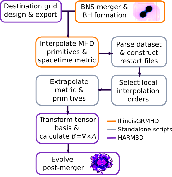
Figure 1: HandOff package workflow. The colors of the borders shows the code responsible for the task, with orange for IllinoisGRMHD, gray for standalone scripts, and purple for Harm3d.

We first describe the GRMHD formalism adopted by both IllinoisGRMHD and Harm3d, as well as the steps performed by the HandOff package that allow us to transition a BNS postmerger simulation from one code to the other. In Fig. 1 we show a sketch of the workflow around the HandOff: We perform a BNS merger simulation until BH formation with IllinoisGRMHD. At the same time, we design and export the numerical grid that we will use to continue the postmerger evolution in Harm3d. We interpolate the MHD primitives and spacetime metric of the postmerger onto this grid, and use these results to construct restart files readable by Harm3d. Then we select results from lower or higher orders of interpolation, depending on the local smoothness of each grid function. If the destination grid is larger than the original grid of IllinoisGRMHD, then we extrapolate the primitives and spacetime metric to populate the complementary cells. Finally, we transform the tensor basis from Cartesian coordinates to the new coordinate system, calculate the magnetic field from the curl of the magnetic vector potential, and continue the postmerger evolution in the new grid with the usual methods of Harm3d.

II.1 GRMHD formalism

The GRMHD formalisms on which IllinoisGRMHD and Harm3d are based are equivalent, but the formulation and conventions adopted by each code differ. Below we present the equations of motion as implemented in Harm3d, and we will describe the differences with IllinoisGRMHD when presenting the methods adopted for the BNS merger.

The evolution of the MHD fields follows from the integration of the general relativistic equations of motion for a perfect fluid with infinite conductivity (ideal MHD). These are the continuity equation, the local conservation of energy and momentum, and Maxwell’s equations [see, for instance, Refs. 80, 79, 82, 81]. In flux-conservative form, they read:

$$\partial_{t}\mathbf{U}(\mathbf{P})=-\partial_{i}\mathbf{F}^{i}+\mathbf{S}(\mathbf{P})\,,$$ (1)

where $\mathbf{P}$ is the vector of primitive variables, $\mathbf{U}$ the vector of conserved variables, $\mathbf{F}$ the fluxes, and $\mathbf{S}$ the sources:

$$\mathbf{P}=\left[\rho,p,\tilde{v}^{k},B^{k}\right]^{\mathrm{T}},$$ (2)

$$\mathbf{U}(\mathbf{P})=\sqrt{-g}\left[\rho u^{t},{T^{t}}_{t}+\rho u^{t},{T^{t}}_{j},B^{k}\right]^{\mathrm{T}},$$ (3)

$$\mathbf{F}^{i}(\mathbf{P})=\sqrt{-g}\left[\rho u^{i},{T^{i}}_{t}+\rho u^{i},\right.\left.{T^{i}}_{j},\left(b^{i}u^{k}-b^{k}u^{i}\right)\right]^{\mathrm{T}},$$ (4)

$$\mathbf{S}(\mathbf{P})=\sqrt{-g}\left[0,{T^{\kappa}}_{\lambda}{\Gamma^{\lambda}}_{t\kappa},\right.\left.{T^{\kappa}}_{\lambda}{\Gamma^{\lambda}}_{j\kappa},0^{k}\right]^{\mathrm{T}},$$ (5)

where $g$ denotes the determinant of the metric, $\rho$ is the rest mass density, $p$ is the fluid pressure, $u^{\mu}$ is the fluid four-velocity, and $\tilde{v}^{k}$ is the fluid velocity as measured by normal observers with four-velocity $n_{\mu}=(-\alpha,\vec{0})$, $\alpha=\sqrt{-1/g^{tt}}$, with $g^{\mu\nu}$ ($g_{\mu\nu}$) the contravariant (covariant) components of the spacetime metric. The magnetic field is represented by $B^{k}={}^{*}F^{kt}$, where ${}^{*}F^{\mu\nu}$ is the dual of the Maxwell tensor times $1/\sqrt{4\pi}$, $b^{\mu}=\left(\delta^{\mu}_{\nu}+u^{\mu}u_{\nu}\right)B^{\nu}/u^{t}$ is the projection of the magnetic field into the fluid’s comoving frame. In addition, ${\Gamma^{\lambda}}_{\mu\nu}$ is the affine connection and ${T^{\mu}}_{\nu}$ is the sum of the stress-energy tensor of a perfect fluid and the EM stress energy tensor, defined as:

$$T_{\mu\nu}=\left(\rho h+2{p_{\mathrm{m}}}\right)u_{\mu}u_{\nu}+\left(p+{p_{\mathrm{m}}}\right)g_{\mu\nu}-b_{\mu}b_{\nu}\,,$$ (6)

where $h=1+\epsilon+p/\rho$ denotes the specific enthalpy, $\epsilon$ the specific internal energy, and ${p_{\mathrm{m}}}=b^{\mu}b_{\mu}/2$ the magnetic pressure. The internal energy is $u=\rho\epsilon$, and we assume an adiabatic $\Gamma$-law equation of state: $p=(\Gamma-1)u$.

The HandOff package can be extended to deal with more general formalisms. For instance, if using a realistic and finite-temperature equation of state, we can also include the electron fraction and temperature of the plasma. We will describe such extensions to the HandOff package in an forthcoming article, where we will transition a simulation from IllinoisGRMHD to the numerical code HARM3D+NUC [81].

II.2 BNS merger

We simulate the BNS merger with the numerical code IllinoisGRMHD [79]. This code is implemented as a set of modules, or “thorns”, built upon the Cactus and Carpet infrastructure [84, 85], within the Einstein Toolkit framework [86, 87]. Carpet enables IllinoisGRMHD to sample the physical fields on Cartesian AMR numerical grids.

The integration in time of the conservation equations for the primitives $\rho,\ p,$ and $\tilde{v}^{k}$ follows from high-resolution shock-capturing (HRSC) schemes. To be precise, IllinoisGRMHD adopts the coordinate velocity $v^{k}=u^{k}/u^{0}$ as a primitive instead of $\tilde{v}^{k}$. HRSC schemes, in a nutshell, reconstruct the primitive variables at the cell interfaces, solve for the fluxes with an approximate Riemann solver, and integrate in time with the Method of Lines (MoL). The standard methods adopted are Piecewise Parabolic Method (PPM) [88] for the reconstruction of primitives, Harten-Lax-van Leer (HLL) for the approximate Riemann solver, and fourth-order Runge-Kutta (RK4) for the MoL integration.

The integration of the induction equation for $B^{k}$ requires further care because the propagation of truncation errors can violate the solenoidal constraint $\partial_{i}\left(\sqrt{-g}B^{i}\right)=0$. Constrained-transport schemes for $B^{k}$ have proven to avoid these violations by finite-differencing the derivatives in the induction equation with specific stencils [see, for instance, 89], but their scope is limited to uniform grids, unless special steps or conditions are implemented. IllinoisGRMHD instead evolves the vector potential $A_{k}$ directly at staggered locations on a given cell, ensuring that results match those adopting a standard constrained-transport algorithm [90]. The algorithm is summarized as follows. The induction equation is recast as an evolution equation for $A_{k}$, which is integrated with HRSC methods, and then $B^{k}$ is obtained from the curl of $A_{k}$, satisfying the solenoidal constraint to roundoff error .

After each time step, the primitive variables need to be recovered from the conserved variables in the conservative-to-primitive step. IllinoisGRMHD adopts a Newton-Raphson-based 2D recovery scheme, which is also available in Harm3d [92]. This step can fail, however, if the conserved variables become invalid during the evolution. This happens most often in regions where high accuracy is difficult to maintain: the low density “atmosphere”, inside the BH horizon, or at AMR refinement boundaries. IllinoisGRMHD enforces MHD inequalities that the conserved variables must satisfy in order to mitigate the number of recovery failures. If a failure still occurs, a backup primitive recovery method is used that is guaranteed to succeed, as described in Appendix A of [93].

The conservative-to-primitive step is prone to failure for lower densities of the artificial atmosphere. A typical value that results in robust, stable evolutions with small numbers of recovery failures is $\rho^{\mathrm{Cactus}}_{\mathrm{atm}}\sim 10^{-8}\rho_{\mathrm{max}}$, where $\rho_{\mathrm{max}}$ is the maximum initial baryonic density. The minimum allowed value for the conserved energy used by IllinoisGRMHD,

$$\tau\equiv\sqrt{-g}\left(\alpha T^{tt}-u^{t}\rho\right),$$ (7)

is obtained by assuming $\rho=\rho^{\mathrm{Cactus}}_{\rm atm}$, flat space, zero velocities, and zero magnetic fields, yielding

$$\tau_{\rm min}=\epsilon^{\mathrm{Cactus}}_{\rm atm}\rho^{\mathrm{Cactus}}_{\rm atm},$$ (8)

where the “atmosphere” energy $\epsilon^{\mathrm{Cactus}}_{\rm atm}=\epsilon(\rho_{\rm atm})$ is computed using the gamma-law EOS with $\Gamma=2$ and $K=0.0332\rho_{\rm nuc}c^{2}/n_{\rm nuc}^{\Gamma}=123.6$ (in code units), where $\rho_{\rm nuc}$ and $n_{\rm nuc}$ are the nuclear rest-mass and number densities, respectively. Empirically, we have determined that choosing an “atmosphere” value $\tau^{\mathrm{Cactus}}_{\rm atm}$ up to ${\sim}10^{2}\tau_{\rm min}$ (see Eq. (8)) leads to stable evolutions and accurate data transfers to Harm3d, while choosing values a few orders of magnitude larger can lead to an unstable transition.

During the BNS merger, the spacetime is highly dynamical and, besides integrating the equations of motion for the plasma, we need to integrate the equations of motion for the metric components $g_{\mu\nu}$. These equations are the Einstein field equations, written in the standard 3+1 Arnowitt-Deser-Misner (ADM) formalism [94], in the BSSNOK formulation [95, 96, 97]. In order to integrate these equations numerically, we use the thorn McLachlan [99], which has been written with the Kranc application.

II.3 Grid design and export

Numerical errors rapidly sap angular momentum from fluid flows that obliquely cross coordinate lines. Thus continuing to model the dynamics of a postmerger BH accretion disk over timescales far longer than the inspiral/merger timescale with moderate-resolution Cartesian AMR grids would be ill advised. Thus we choose a post-handoff grid that samples the remnant accretion disk in a spherical coordinate system designed specifically for modeling black hole accretion. The post-handoff grid is implemented within the same code adopted for post-handoff evolution: Harm3d.

To begin the handoff, Harm3d specifies the Cartesian coordinate locations of all cell centers, lower faces, and corners, for both physical and ghost cells on its spherical grid. The number of coordinates dumped, then, is $\left(N^{r}+2N_{\mathrm{G}}\right)\times\left(N^{\theta}+2N_{\mathrm{G}}\right)\times\left(N^{\phi}+2N_{\mathrm{G}}\right)\times 3\times 5$, where $N^{r}$, $N^{\theta}$, and $N^{\phi}$ are the number of cells in each dimension, $N_{\mathrm{G}}$ is the number of ghost cells beyond each coordinate boundary, $\times 3$ stands for each spatial dimension, and $\times 5$ for each cell location.

In case the numerical codes assume different values for the unity of mass in geometrical units, we normalize the exported coordinates. For instance, if the unit of length of the destination grid equals the mass of the black hole remnant $M_{\mathrm{BH}}$, but the unit of length during the merger equals $M_{\odot}$, then we multiply the exported coordinates of the destination grid by $M_{\mathrm{BH}}/M_{\odot}$.

II.4 Interpolation routine

In order to restart a GRMHD simulation in Harm3d we need two sets of grid functions at a given time: the MHD primitives $\mathbf{P}_{\mathrm{HandOff}}$, and the geometry of spacetime $\mathbf{g}_{\mathrm{HandOff}}$. We have implemented a thorn within the Cactus infrastructure that reads in the Cartesian coordinates of the cell positions of the destination grid and proceeds to interpolate both sets of grid functions into them.

Specifically, regarding the first set $\mathbf{P}_{\mathrm{HandOff}}$, we interpolate the following grid functions:

$$\mathbf{P}_{\mathrm{HandOff}}=\left\{\rho,p,\tilde{v}^{r},\tilde{v}^{\theta},\tilde{v}^{\phi},A_{x},A_{y},A_{z}\right\}.$$ (9)

We require most of the values of $\mathbf{P}_{\mathrm{HandOff}}$ only at the cell centers and, since their behavior can be smooth or discontinuous, we use three different orders of Lagrangian interpolation: first, second, and fourth. The vector potential components $A_{k}$ are an exception: To be consistent with the algorithms that calculate the curl of $A_{k}$ in Harm3d, we interpolate the components of $A_{k}$ into the corners of the destination cells. Further, we use third-order Hermite interpolation for $A_{k}$ since it ensures continuity in the first derivatives of the interpolant function. Notice that, although we will transform the basis of tensorial quantities later in the HandOff, we transform the Cartesian velocities $\left\{v^{x},v^{y},v^{z}\right\}$ to a spherical basis $\left\{v^{r},v^{\theta},v^{\phi}\right\}$ before interpolation. In this way, we avoid the propagation of truncation errors of dominant components—usually $\tilde{v}^{\phi}$—into other components during the basis transformation.

Regarding the second set, $\mathbf{g}_{\mathrm{HandOff}}$, consider that Harm3d does not evolve the spacetime metric, so the HandOff is limited to stationary geometries. Then $\mathbf{g}_{\mathrm{HandOff}}$ is simply given by the components of the four-dimensional metric in Cartesian coordinates:

$$\mathbf{g}_{\mathrm{HandOff}}=\left\{g_{\mu\nu}^{\mathrm{Cart}},\ \mu,\nu=t,x,y,z\right\}.$$ (10)

We interpolate $\mathbf{g}_{\mathrm{HandOff}}$ to every cell position and, since the metric components will be differentiated for the calculation of the affine connections, we use third-order Hermite interpolation that, as mentioned, ensures continuity in the first derivatives of the interpolant function.

Even in the equal-mass case, the collapsed BH after a BNS merger might have a gauge-induced velocity $\tilde{v}^{i}_{\mathrm{BH}}$. We correct for this effect by applying the interpolation routine in the frame of the BH. Specifically, we shift $x^{i}\rightarrow x^{i}-x^{i}_{\mathrm{BH}}$ and $\beta^{i}\rightarrow\beta^{i}+\tilde{v}^{i}_{\mathrm{BH}}$ before calculating and interpolating $\mathbf{P}_{\mathrm{HandOff}}$ and $\mathbf{g}_{\mathrm{HandOff}}$.

If the radial extent of the destination grid exceeds the boundaries of IllinoisGRMHD’s grid, then we set the grid functions to an undefined value, or NaN, at the corresponding cells. Marking cells in this way ensures that they are easily found and their values overwritten with extrapolated data later in the HandOff procedure.

The interpolation routine returns a unique file in binary format where the values of each grid function in the destination grid are stored in contiguous memory locations.

II.5 Parse dataset

With a standalone script, we parse the binary file that results from the interpolation routine, and construct restart files, readable by Harm3d. Specifically, we read each grid function and distribute it in an array of dimension $(N^{r}+2N_{\mathrm{G}},N^{\theta}+2N_{\mathrm{G}},N^{\phi}+2N_{\mathrm{G}})$. We discard the values of the primitives at the ghost cells as we will refill them at runtime based on the boundary conditions selected for the continued evolution. The vector potential $A_{k}$ entails an exception: We need to keep its interpolated values at the ghosts cells in order to calculate its curl when initializing the continued run. We also keep the interpolated values of the metric at the ghost cells, since these will be required at initialization for calculating the spacetime connections in the physical cells next to the coordinate boundaries.

We dump these reordered arrays in three restart files, each containing a different interpolation order for the primitives $\mathbf{P}_{\mathrm{HandOff}}$.

II.6 Selective interpolation orders

The truncation errors in an interpolation scheme over a smooth function are proportional to $\Delta x^{n+1}$, where $\Delta x$ denotes a measure of the grid resolution and $n$ the order of the algorithm. Higher orders are preferred for smooth functions to minimize the truncation error. MHD primitives, however, might present strong shocks and discontinuities that induce Gibbs phenomena when using high interpolation orders. Our strategy in the HandOff is to keep higher-order results where the solution is smooth, but lower-order results where it is sharp. To that end, for each primitive, we take the results from the first-order interpolation, which is free of Gibbs phenomena, and we compare its local values to the averages over its neighboring cells ($\pm 2$ cells in each dimension). If the relative error between these quantities is lower than $1\%$, then we take the local result from the fourth-order interpolation; if it is higher than $10\%$, then we take the first-order result; and if it is in between, then we take the second-order result. The final outcome of this step is a unique restart file that mixes first-, second-, and fourth-order results for the primitives $\mathbf{P}_{\mathrm{HandOff}}$.

This step is crucial for the robustness and precision of the HandOff. During our testing stage, we found that higher-order methods can introduce Gibbs phenomena in the MHD primitives at the boundaries of handed-off accretion disks, leading to severe MHD perturbations and shocks that were not in the original simulation, and preventing a continuous transition between codes. On the other hand, using solely lower-order methods compromised the accuracy of the transition.

II.7 Metric and primitives extrapolation

In case the outer boundary of the destination grid exceeds the outer boundary of the original grid, we extrapolate the geometry $\mathbf{g}_{\mathrm{HandOff}}$ and primitives $\mathbf{P}_{\mathrm{HandOff}}$ into the complementary cells.

Regarding the geometry $\mathbf{g}_{\mathrm{HandOff}}$, we treat each of the ten independent components of the four-metric individually. Unlike the primitives $\mathbf{P}_{\mathrm{HandOff}}$, the metric components will generally take nonzero values everywhere in the computational domain, falling off as inverse polynomials of radius. To extrapolate each metric component $g_{\mu\nu}$ out to the larger computational domain, we follow this procedure:

• Perform a low-order (up to $(l,m)=(4,\pm 4)$) spherical harmonic mode decomposition of the component at each radius $r$ in the destination grid The result is a radial array of mode coefficients $g_{\mu\nu}^{(l,m)}(r)\equiv\oint g_{\mu\nu}(r,\theta,\phi)Y_{lm}(\theta,\phi)d\Omega$.

• In a “trusted window” $r\in\{R_{1},R_{2}\}$, perform a least-squares fit of each mode coefficient $g_{\mu\nu}^{(l,m)}(r)$ to a power-law function $a_{0}+a_{1}/r^{n}$.

• Construct a new radial array of coefficients that transitions continuously from the original numerical data to the power-law fit over the course of the trusted window:

  $$\bar{g}_{\mu\nu}^{(l,m)}(r)=(1-\lambda(r))g_{\mu\nu}^{(l,m)}(r)+\lambda(r)(a_{0}+a_{1}/r^{n}),$$

  where

  $$\lambda(r)\equiv\begin{cases}0&r<R_{1}\\ \frac{r-R_{1}}{R_{2}-R_{1}}&R_{1}\leq r\leq R_{2}\\ 1&r>R_{2}\end{cases}$$

• Use the power-law fit to generate $g_{\mu\nu}^{(l,m)}(r)$ values for all $r>R_{2}$, extending to fill the full Harm3d domain.

• Finally, reconstruct $g_{\mu\nu}(r,\theta,\phi)$ at every point in the larger domain using the new extended $g_{\mu\nu}^{(l,m)}(r)$.

For some individual modes, the power-law functional least-squares fit may fail to converge—generally a symptom of that mode being dominated by low-amplitude noise. In these cases, we keep the original mode data out to $R_{2}$, and use the value at $r=R_{2}$ to fill the remainder of the domain—equivalent to setting $a_{0}=g_{\mu\nu}^{(l,m)}(R_{2}),a_{1}=0$.

After extrapolating the metric components, we proceed to extrapolate the primitives $\mathbf{P}_{\mathrm{HandOff}}$. We fill the complementary cells with the numerical atmosphere of Harm3d, $\rho=\rho_{\mathrm{atm}}$, $u=u_{\mathrm{atm}}$, where $\rho_{\mathrm{atm}},u_{\mathrm{atm}}$ are defined below, and we set the rest of the primitives to zero.

To avoid a sharp transition between the numerical atmospheres of IllinoisGRMHD and Harm3d at the the boundary between the handed-off and extrapolated primitives, we also adjust the handed-off atmosphere. If $\rho<1.1\times\rho_{\mathrm{atm}}^{\mathrm{Cactus}}$, we set $\rho=\rho_{\mathrm{atm}}$, $u=u_{\mathrm{atm}}$, and keep the rest of the primitives unchanged.

II.8 Continued evolution

At this stage we have a restart file in a format readable by Harm3d that contains the MHD primitives at the physical cell centers, the vector potential $A^{k}$ at the corners of physical and ghost cells, and the metric at all cell positions for all cells. Using existing restart routines, we read in and distribute the MHD primitives among different processors in Harm3d. The vector potential and metric components require specific routines that take into account the ghost cells and different cell positions when reading in and distributing its values.

We transform the metric and vector potential components from the Cartesian basis to the numerical basis of the destination grid:

$$g_{\mu^{\prime}\nu^{\prime}}=\frac{dx^{\alpha}_{\mathrm{Cart}}}{dx^{\mu^{\prime}}}\frac{dx^{\beta}_{\mathrm{Cart}}}{dx^{\nu^{\prime}}}g_{\alpha\beta}^{\mathrm{Cart}}\,,$$ (11)

$$A_{\mu^{\prime}}=\frac{dx^{\alpha}_{\mathrm{Cart}}}{dx^{\mu^{\prime}}}A_{\alpha}^{\mathrm{Cart}}\,,$$ (12)

and we transform the velocity from the spherical basis to numerical:

$$\tilde{v}^{\mu^{\prime}}=\frac{dx^{\mu^{\prime}}}{dx^{\alpha}_{\mathrm{sph}}}\tilde{v}^{\alpha}_{\mathrm{sph}}\,.$$ (13)

We calculate the curl of the vector potential $A_{k}$ with standard routines in Harm3d and obtain the magnetic field $B^{k}$ at the cell centers, maintaining the solenoidal constraint [102]. We also calculate the affine connections for the numerical metric with standard routines of Harm3d. These use fourth-order (second-order) finite differences for spatial (temporal) derivatives of the metric to obtain the Christöffel symbols; cell extents are used as the discrete spacing in the spatial finite differences, while a much smaller time spacing than the evolution’s Courant-limited time step is used in order to keep its truncation error smaller than that of the spatial difference. We typically limit the simulations from handed-off initial data (ID) to instances when the metric is nearly stationary, so the continued evolution is assumed to have a time-independent spacetime. For this reason during HandOff we simply use the same metric field data for all nominal time slices fed into the Harm3d affine connection routine, guaranteeing that all temporal derivatives will be zero.

We evolve the handed-off primitives over the numerical spacetime in the destination grid with the well-tested methods of Harm3d [103, 80, 81]. We integrate the equations of motion, Eq. (1), with HRSC schemes. We reconstruct the primitive variables to the cell interfaces through piecewise parabolic interpolation, we apply the Lax-Friedrichs formula to compute the local fluxes, and the method of lines for time integration with a second-order Runge-Kutta (RK2) method. The primitive variables are recovered from the conserved variables with the scheme described in [92, 81]. If the updates of $\rho$ or $u$ go below the corresponding atmosphere values $\rho_{\mathrm{atm}}=2\times 10^{-10}(r/M)^{-3/2}$, $u_{\mathrm{atm}}=2\times 10^{-12}(r/M)^{-5/2}$ they are reset to the latter. We use the constrained transport algorithm FluxCT [89] to evolve the magnetic field $B^{k}$ and maintain the solenoidal constraint. For more details, see Ref. [80].

III Code Verification: Fishbone-Moncrief disk

To verify the HandOff we take the case of a magnetized Fishbone-Moncrief (FM) disk [104] around a rotating BH. We evolve the system with IllinoisGRMHD and Harm3d independently, and we use the HandOff to perform several transitions between the codes at different stages of the simulation.

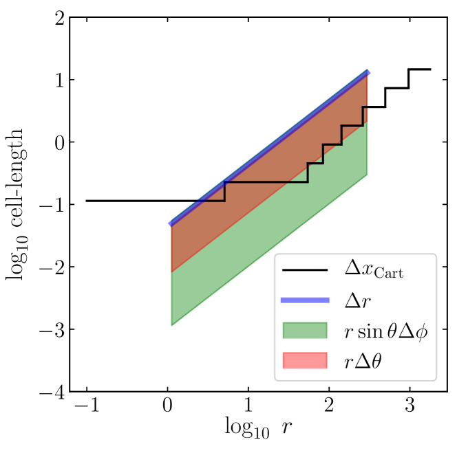
Figure 2: Cell lengths as a function of radii for the FM simulations in IllinoisGRMHD (black) and Harm3d (green, red, and blue). Shaded regions show how the cell lengths change over the full span of $\theta$. Note that regions of overlap between green and red appear brown in the plot.

We begin by setting the same initial data in IllinoisGRMHD and Harm3d for a magnetized FM disk around a BH of mass $M$ with specific angular momentum $a/M=0.9375$, as dictated by Ref. [105]. We evolve this data with IllinoisGRMHD and Harm3d up to $t=10^{4}M$. The grid in IllinoisGRMHD consists of a Cartesian hierarchy of eight refinement levels, as described in Ref. [105]. The grid in Harm3d has a spherical topology and consists of $128^{3}$ cells, parametrized by numerical coordinates that refine the resolution towards the equator and towards the BH, with the functional dependence used by Ref. [106] (we use $h=0.3$ in Eq. (8) of this reference). We make use of novel boundary conditions at the coordinate boundaries of $\theta$, i.e. at the polar axis, which allow us to fully extend $\theta\in(0,\pi)$. In Appendix B we describe the details of these boundary conditions. The coordinate boundaries of $\phi$ are internal to the domain, and the coordinate boundaries of $r\in\left[1.1M,300M\right]$ are physical boundaries, where we impose outflow boundary conditions.

In Fig. 2 we plot the cell lengths in both IllinoisGRMHD and Harm3d as a function of radii and for $\theta\in(0,\pi)$, and conclude the resolutions are comparable. The cell length $\Delta r$ grows as a function of radius because the radial resolution has an exponential dependence with radius. The cell length $r\sin\theta\Delta\phi$ grows as a function of radius because of its explicit radial dependence, and also spans different values at each radius because of its $\theta$ dependence. Finally the cell length $r\Delta\theta$ grows as a function of radius because of its explicit radial dependence and has different values for a given radius because $\Delta\theta$ is not uniform, but progressively smaller toward the equator. Such flexibility of the numerical grids in Harm3d to adapt optimally to the relevant physical processes is one of the main motivations behind the HandOff. In this case, the numerical grid in Harm3d has less than $\times 80$ cells than the numerical grid in IllinoisGRMHD and will bring comparable results.

As can be seen from Fig. 2, the numerical domain in Harm3d is contained in the domain in IllinoisGRMHD, therefore we do not need to extrapolate the primitives or metric (see Sec. II.7). We will validate the extrapolation procedure in the next section, where we apply the HandOff to a BNS postmerger.

We do the first transition at $t=0$, i.e. we hand off the initial data (ID) from IllinoisGRMHD to Harm3d. By comparing the resulting dataset with the ID constructed in Harm3d, we can measure the truncation error introduced in the HandOff. Based on the resolution of IllinoisGRMHD in the region of the disk $\Delta x_{\mathrm{IGM}}\approx 0.2274$, and the interpolation orders considered $n=1,2,3,4$, we expect the following values for the truncation errors

$$\epsilon\sim\Delta x_{\mathrm{IGM}}^{n+1}\sim\begin{cases}5\times 10^{-2},\ n=1\\ 1\times 10^{-2},\ n=2\\ 2\times 10^{-3},\ n=3\\ 6\times 10^{-4},\ n=4\end{cases}\,.$$ (14)

In Fig. 3 (left) we plot the interpolation orders selected for the primitive $\rho$, in the $xz$ plane. The distribution follows the expected behavior: At the core of the disk, around the position of the maximum of pressure at $r=12M$, fourth order interpolation is selected. In contrast, at the surface of the disk, where the density jumps to the value of the numerical floor, first order is selected. There is also a transition region in the body of the disk where second order is selected.

In Fig. 3 (right) we plot $\epsilon_{\mathrm{R}}[\rho]$ in the $xz$ plane, where

$$\epsilon_{\mathrm{R}}[P]=\frac{\left|P_{\mathrm{harm3d}}-P_{\mathrm{HandOff}}\right|}{\frac{1}{2}\left(\left|P_{\mathrm{harm3d}}\right|+\left|P_{\mathrm{HandOff}}\right|\right)}$$ (15)

is the relative error between the handed-off primitive and the value initialized in Harm3d. As expected from the estimates in Eq. (14), the body of the disk presents $\epsilon_{\mathrm{R}}[\rho]\sim 1\times 10^{-4}$ and transitions to $\epsilon_{\mathrm{R}}[\rho]\sim 1\times 10^{-2}$ near the surface of the disk. The region around the BH with higher errors happens because IllinoisGRMHD sets a tenuous atmosphere with $\rho>1.1\rho_{\mathrm{atm}}^{\mathrm{Cactus}}$ around the BH and the HandOff does not reset it to the Harm3d’s atmosphere. This is still a low-density region, where $\rho<1\times 10^{-5}$ in code units, and it does not affect our results. In global terms, the density-weighted relative error $\left<\epsilon_{\mathrm{R}}[\rho]\right>_{\rho}$, where

$$\left<X\right>_{\rho}=\frac{\int X\rho\sqrt{-g}\,dV}{\int\rho\sqrt{-g}\,dV},$$ (16)

is $\left<\epsilon_{\mathrm{R}}[\rho]\right>_{\rho}=2\times 10^{-4}$.

For the remaining primitives, we find equivalent distributions for the interpolation orders selected, but different values for the integrated errors. We find a higher integrated error for the internal energy $\left<\epsilon_{\mathrm{R}}[u]\right>_{\rho}=1\times 10^{-2}$ but this is dominated by random perturbations, introduced artificially to trigger accretion. We find lower errors for nonvanishing components of the velocity $\left<\epsilon_{\mathrm{R}}[v^{(1)}]\right>_{\rho}=8\times 10^{-6}$ and $\left<\epsilon_{\mathrm{R}}[v^{(3)}]\right>_{\rho}=1\times 10^{-5}$. These functions are smoother than $\rho$, and monotonically decrease in $r$ within the disk, explaining why the interpolation is more accurate. We find higher errors for the nonvanishing components of the magnetic field $\left<\epsilon_{\mathrm{R}}[B^{(1)}]\right>_{\rho}=\left<\epsilon_{\mathrm{R}}[B^{(2)}]\right>_{\rho}=1\times 10^{-1}$ that come from the propagation of truncation errors in $A_{k}^{\mathrm{Cart}}$ after the basis transformation and curl calculation. Regarding the primitives that are initialized to zero, we define the relative error by

$$\tilde{\epsilon}_{\mathrm{R}}[P]=\left|P_{\mathrm{HandOff}}\right|$$ (17)

and find $\left<\tilde{\epsilon}_{\mathrm{R}}[v^{(2)}]\right>_{\rho}=5\times 10^{-19}$ and $\left<\tilde{\epsilon}_{\mathrm{R}}[B^{(3)}]\right>_{\rho}=4\times 10^{-8}$. Comparing $\left<\tilde{\epsilon}_{\mathrm{R}}[v^{(2)}]\right>_{\rho}$ with $\left<\tilde{\epsilon}_{\mathrm{R}}[B^{(3)}]\right>_{\rho}$ we notice the convenience of transforming to the spherical basis before interpolation and the effect of error propagation by the curl calculation. In the case of the BNS postmerger, however, we expect these errors on the magnetic field components to be smaller, since the different components, and therefore the truncation errors, will be more comparable in magnitude.

In this validation test, we can also measure the truncation errors of the handed-off metric components , since we know their analytical values in advance. Overall, we find lower errors for the metric components than for the MHD primitives, $\left<\epsilon_{\mathrm{R}}[g_{\mu\nu}]\right>_{\rho}<1\times 10^{-7}$. These lower errors in the metric components were expected because these are differentiable functions, and because we use third-order interpolation in every cell.

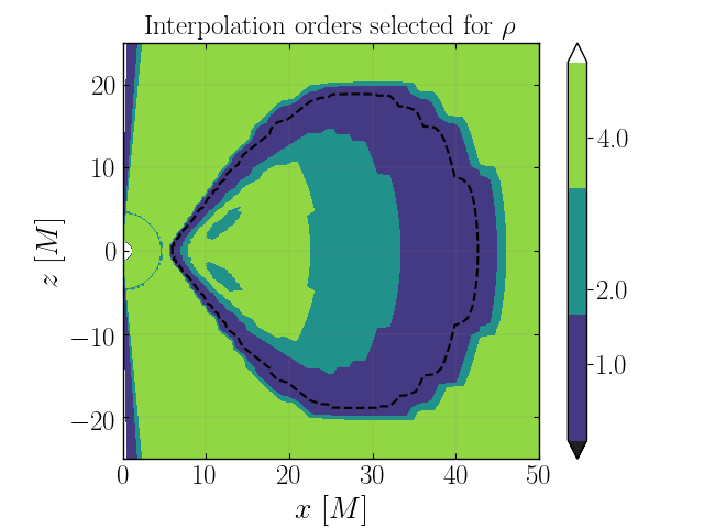
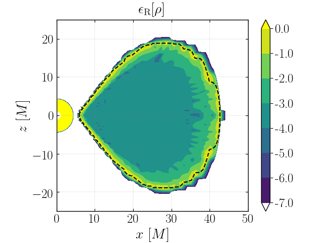
Figure 3: Interpolation orders selected (left) and the correspoding relative errors (right) for $\rho$, when handing-off ID for a magnetized FM from IllinoisGRMHD to Harm3d. Fourth order interpolation is selected at the core of the disk where $\rho$ is smooth, and first order interpolation is selected at the surface of the disk where there is a jump to the numerical floor. There is also a transition region where second order interpolation is selected. The numerical errors follow the expected values from the resolution and interpolation orders (see Eq. (14)).

After confirming that the handed-off ID and spacetime metric are consistent with our expectations, we evolve the dataset within Harm3d. We denote this simulation HandOff_0.

Defining the accretion rate as

$$-\frac{dM}{dt}(r)=\int\rho u^{r}\sqrt{-g}\,d\theta\,d\phi,$$ (18)

in Fig. 4 (top) we plot this quantity at the BH horizon for HandOff_0 (green) and for the fiducial run in Harm3d (light blue). We also include the accretion rate for the fiducial run in IllinoisGRMHD (orange). We notice the evolution of HandOff_0 is dynamically equivalent to the fiducial run in Harm3d, capturing the MRI growth, saturation, and relaxation.

To test the HandOff in a more realistic and turbulent scenario, we transition the same simulation from IllinoisGRMHD to Harm3d at $t=4.1\times 10^{3}M$. We denote this continued evolution HandOff_1. In Fig. 4 (top, red) we plot the resulting accretion rate and, again, we find the HandOff succesfully captures the dynamical state of the disk, reproducing the value of the accretion rate at the time of transition, and the spike in the accretion rate at $t\sim 5\times 10^{3}M$.

Finally, we perform a transition at $t=8.1\times 10^{3}M$ and we denote this continued evolution HandOff_2. In Fig. 4 (top, violet) we plot the resulting accretion rate and we notice its value at the transition time matches the value in IllinoisGRMHD, proving a continuous transition. The accretion rate then converges to the results of Harm3d. Indeed, while the state of the disk at the transition time is determined by IllinoisGRMHD, the continued evolution is determined by the numerical methods in Harm3d.

Beyond the local measure of the accretion rate, we analyze the continuity of global quantities after the HandOff. In Fig. 4 (bottom) we plot the integrated mass of the disk within $r=100M$, normalized by the initial mass $M_{0}$. We find the curves of HandOff_0, HandOff_1 and HandOff_2 match the results from IllinoisGRMHD at the time of transition, proving the high fidelity of the HandOff.

We conclude the HandOff succesfully translates the GRMHD state of a magnetized torus, and the spacetime metric, from a Cartesian-AMR grid within IllinoisGRMHD to a more flexible grid within Harm3d. In the next section we will apply the HandOff to the interesting case of a BNS postmerger.

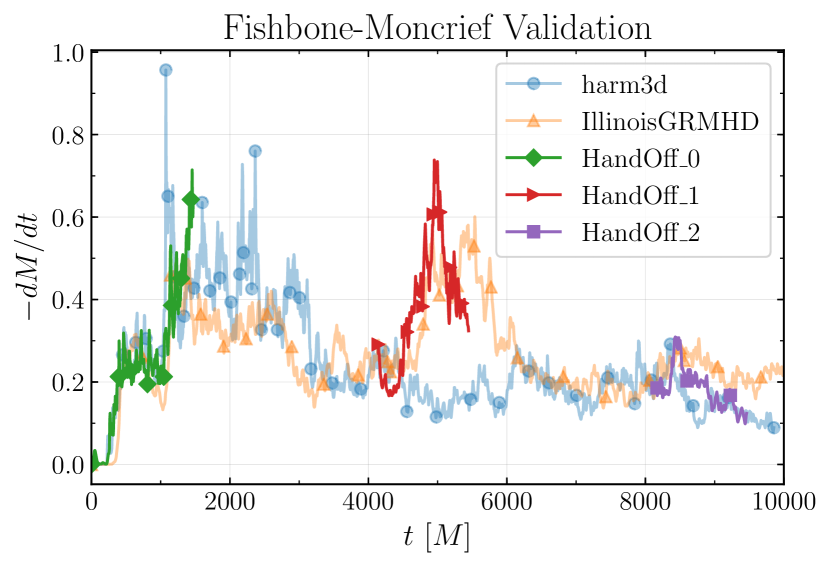
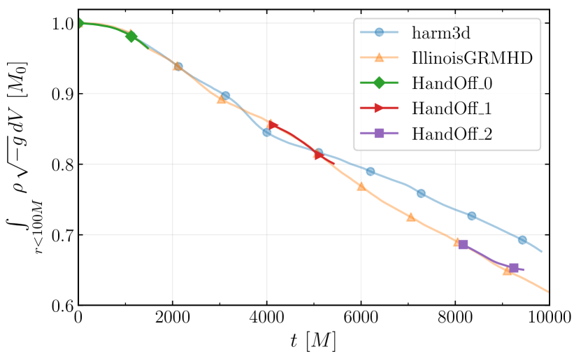
Figure 4: Accretion rate at the horizon (top) and total mass within $r=100M$ (bottom) as a function of time for the FM validation case. The curves harm3d and IllinoisGRMHD stand for the fiducial simulations with these codes. The curves HandOff_0, HandOff_1 and HandOff_2 represent handed-off runs from IllinoisGRMHD to Harm3d, at times $t=0,\ 4.1\times 10^{3},\ 8.1\times 10^{3}M$, respectively. In every case, the transition is continuous and the evolved system follows the expected behavior from the fiducial runs.

IV Results: BNS postmerger

In this section we evolve a BNS merger with IllinoisGRMHD and apply the HandOff to continue the postmerger evolution in Harm3d. The results presented in this section are well known from the literature, but serve to demonstrate the consistency and validity of the continued evolution from the HandOff.

IV.1 Merger proper

The ID for the BNS is similar to that of [58] [see also Refs. 64, 66, for similar settings]: Two NSs in a circular orbit, separated by ${\sim}45~{}\mathrm{km}$, each with a gravitational mass of $1.5~{}M_{\odot}$ and an equatorial radius of $13.6~{}\mathrm{km}$. We also initialize two poloidal magnetic fields, confined in each star, but with a maximum strength of ${\sim}10^{15}~{}\mathrm{G}$, three orders of magnitude higher than in Ref. [58]. We use a Cartesian-AMR grid centered in the center of mass of the system, with outer boundaries at ${\sim}5700~{}\mathrm{km}$, and seven refinement boundaries with a finest resolution of ${\sim}180~{}\mathrm{m}$. We model the fluid as an ideal gas, with adiabatic index $\Gamma=2$.

We evolve this ID with IllinoisGRMHD and, consistent with Ref. [58], we find the NSs inspiral towards the center of mass of the system as they transfer energy and angular momentum to gravitational waves (GWs), until they merge after $8~{}\mathrm{ms}$ (${\sim}3$ orbits). After merger, a HMNS forms but, given the large mass of the system, it promptly collapses to a BH (${\sim}8~{}\mathrm{ms}$ after merger). If we set the ID at time $t=0.0~{}\mathrm{s}$, then the BH forms at $t_{\mathrm{BH}}=0.017~{}\mathrm{s}$. We use the thorn AHFinderDirect [107] to locate the apparent horizon; the resulting BH has a mass of $2.911~{}M_{\odot}$, a specific angular momentum of $0.82$, and a drift velocity $v_{\mathrm{BH}}\sim 1\times 10^{-3}c$. At $t=t_{\mathrm{BH}}$, we add two refinement levels centered at the remnant, yielding a finest resolution after merger of ${\sim}50~{}\mathrm{m}$. The remnant is surrounded by an orbiting and magnetized torus, with mass $0.076~{}M_{\odot}$.

IV.2 Handing off the postmerger: Destination grids and boundary conditions

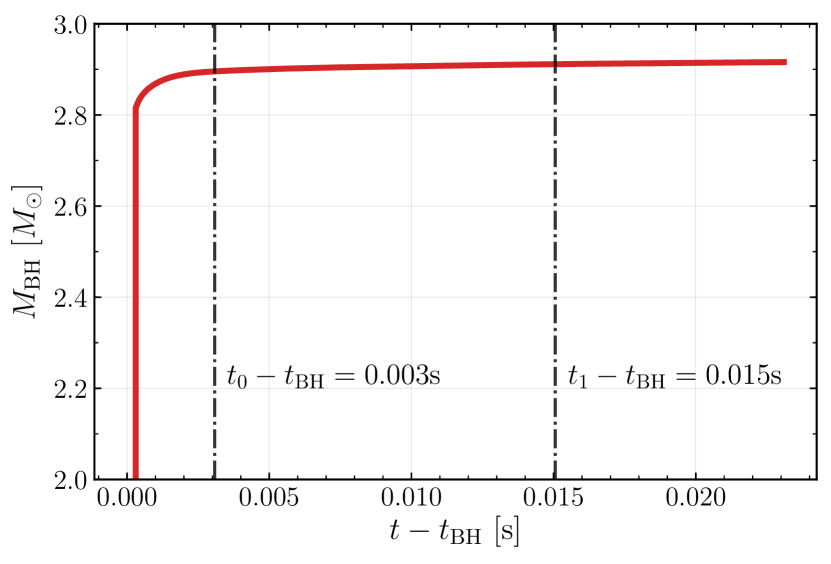
Figure 5: Mass of BH remnant from the BNS merger, as a function of time. Dashed-dotted lines represent the times at which we apply the HandOff. For our fiducial run, $M_{\mathrm{BH}}(t_{1})=2.911M_{\odot}$.

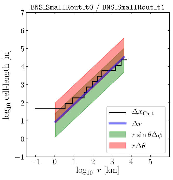
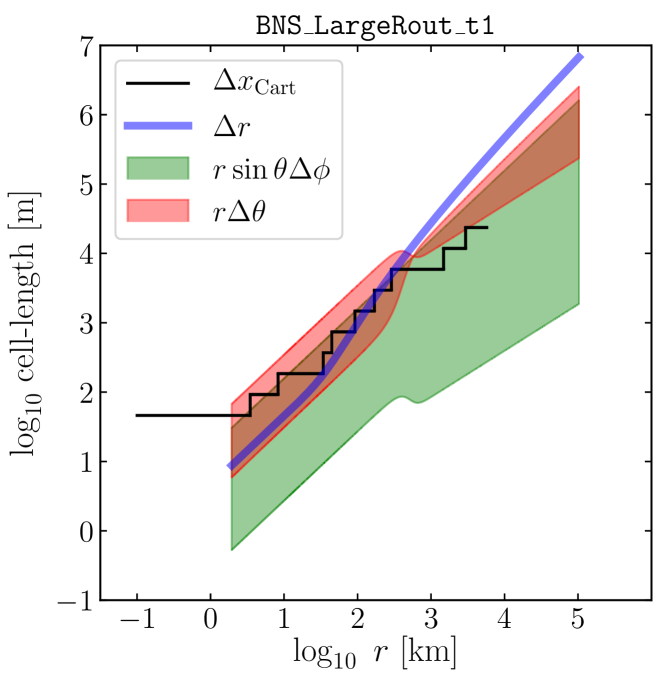
Figure 6: cell lengths for BNS postmerger simulations as a function of radii. The black line represent the resolution of the AMR-levels used during merger. Green, red, and blue points represent the grid lengths for spherical-like cells used during the continued evolution in BNS_SmallRout_t0 (left), BNS_SmallRout_t1 (left), and BNS_LargeRout_t1 (right).

After BH formation, we apply the HandOff and transition the BH-torus system to Harm3d. For consistency checks, we do the transition at different times and to different grids.

We do the first HandOff at $t_{0}=0.020~{}\mathrm{s}$, $0.003~{}\mathrm{s}$ after BH formation, and use a grid equivalent to that of Ref. [108], but with $\xi=0.65$, $\theta_{\mathrm{c}}\sim 1\times 10^{-14}$, and $n=7$ (see Eq. (22) of that reference), we set the radial extent $r\in(1.07,4291.53)~{}\mathrm{km}$, and use $1024\times 160\times 256$ cells. This grid is contained in the original grid for the merger, so we do not need to extrapolate the primitives or spacetime metric. We denote this transition, and continued evolution, BNS_SmallRout_t0. Using this same grid, we do a later transition, at $t_{1}=0.032~{}\mathrm{s}$, denoted BNS_SmallRout_t1. In Fig. 5 we plot the mass of the BH remnant $M_{\mathrm{BH}}$ as a function of time, calculated with the thorn QuasiLocalMeasures [109], and notice that $M_{\mathrm{BH}}$ is in a converging regime at times $t_{0}$ and $t_{1}$. Specifically, $M_{\mathrm{BH}}(t_{0})=2.895M_{\odot}$ and $M_{\mathrm{BH}}(t_{1})=2.911M_{\odot}$.

Next, we do a transition at the same time $t_{1}$, but to a grid designed specifically for a BNS postmerger. As described in the Introduction, this new grid has spherical topology, the outer boundary is far enough (${\sim}10^{5}~{}\mathrm{km}$) to capture the jet breakout, it has higher resolution in $\theta$ towards the equator if close to the BH to resolve the disk, but higher resolution towards the polar axis if farther away, to resolve the funnel region. The implementation details of this grid are described in Appendix A. In this case, since the destination grid is much larger than the original grid for the merger, we need to extrapolate the primitives and spacetime metric to the complementary cells. We denote this run BNS_LargeRout_t1, and consider it our fiducial simulation.

In Fig. 6 we include plots for the cell lengths of these grids as a function of radii and for $\theta\in(0,\pi)$, compared with the resolution in IllinoisGRMHD. We notice that, at the bulk of the disk ($r<200~{}\mathrm{km}$), cells at the equator have higher resolution for both $\theta$ and $r$ with respect to the original resolution in IllinoisGRMHD, and comparable resolution for $\phi$. The description of Fig. 6 (left) is similar to that of Fig. 2 in the previous section, for an exponential grid in $\Delta r$ with $\Delta\theta$ focused in the equator. The description of Fig. 6 (right) is more subtle and is given in Appendix A.

In every case, we apply novel boundary conditions of Harm3d at the polar axis that refer to neighboring cells in the domain, allowing us to extend $\theta\in(0,\pi)$ and to fully resolve the funnel region. See Appendix B for the details on implementing these boundary conditions. The coordinate boundaries of $\phi$ are are also internal to the domain, and the coordinate boundaries of $r$ are the actual physical boundaries, where we impose outflow boundary conditions.

IV.3 Handing off the postmerger: Initial data

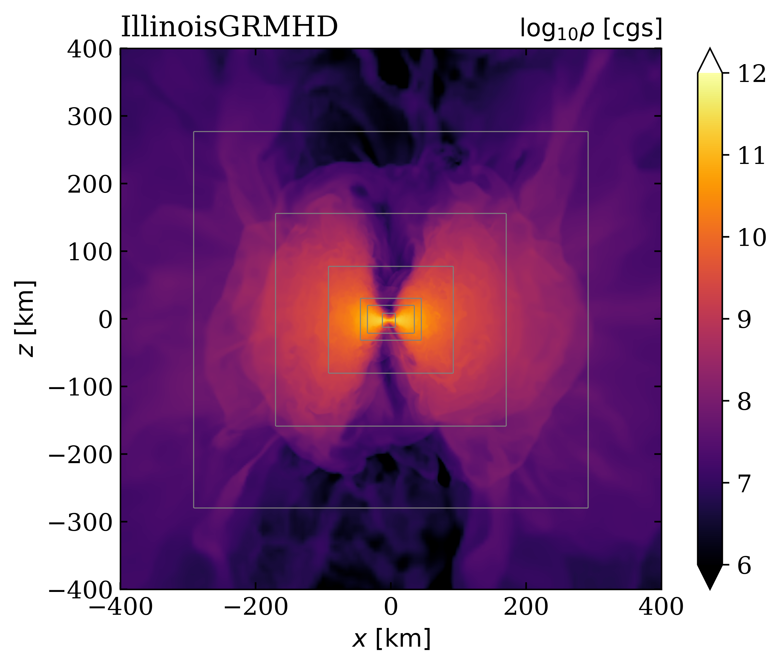
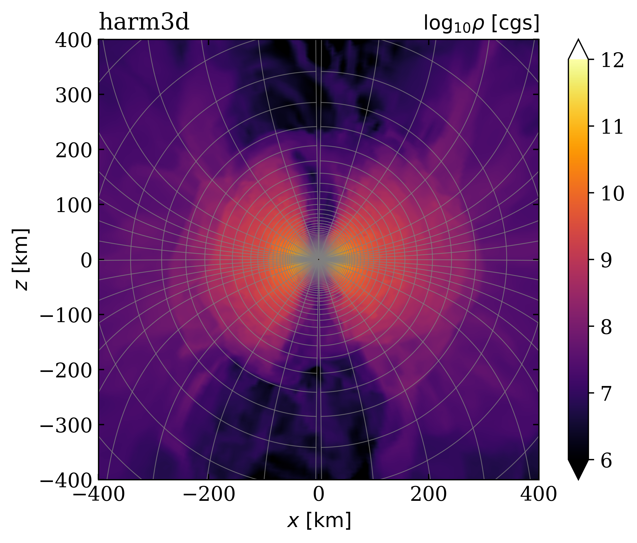
Figure 7: Baryonic density $\rho$ in the $xz$-plane for BNS_LargeRout_t1 before (top) and after (bottom) the hand-off procedure, in IllinoisGRMHD and Harm3d, respectively. The gray lines in the plot for IllinoisGRMHD represent the AMR boundaries and, in the plot for Harm3d, they represent 1 every 10 grid lines of the destination grid.

In Fig. 7 we plot the rest-mass density $\rho$ in the $x-z$ plane at the time of transition for BNS_LargeRout_t1 (bottom). We also plot the original data from IllinoisGRMHD (top), and we plot gray lines that represent the grid topology for each case. As a demonstration of the precision of the HandOff, we note the plots of $\rho$ are indistinguishable between the two codes.

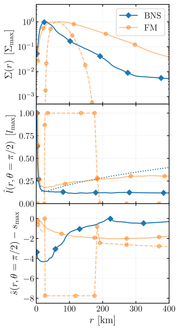
Figure 8: Disk measures for BNS_LargeRout_t1 at the time of transition (solid, diamond, blue), and for the FM disk evolved in Sec. III at $t=0$ (dashed, circle, orange) and $t=9000M$ (solid, circle, orange). From top to bottom, we plot the $\theta$-integrated and $\phi$-averaged density $\Sigma(r)$, the specific angular momentum at the equator $\hat{l}(r,\theta=\pi/2)$, and specific entropy at the equator $\hat{s}(r,\theta=\pi/2)$. The blue, dotted line in the middle panel represent the Keplerian value for $\hat{l}(r,\theta=\pi/2)$, given the mass and spin of the remnant BH.

In Fig. 8 we focus on the accretion disk around the remnant for BNS_LargeRout_t1 (solid, blue), and plot the $\theta$-integrated and $\phi$-averaged density:

$$\Sigma(r)=\frac{\int\sqrt{-g}\rho\,d\theta\,d\phi}{\int\sqrt{g_{\phi\phi}(\theta=\pi/2)}\,d\phi},$$ (19)

and the $\phi$-averaged specific angular momentum $\hat{l}~{}(r,\theta=~{}\pi/2)$ and specific entropy $\hat{s}~{}(r,\theta=~{}\pi/2)$ at the equator, where $l=u_{\phi}/u_{t}$, $s=\ln(p/\rho^{\Gamma})$, and

$$\hat{X}(r,\theta)=\frac{\int X\sqrt{g_{\phi\phi}}\,d\phi}{\int\sqrt{g_{\phi\phi}}\,d\phi}.$$ (20)

Since many references initialize the postmerger disk with an FM distribution [e.g. 110], or similar isentropic solutions with constant specific angular momentum, in Fig. 8 we also plot the latter quantities for the FM disk evolved in the previous section at $t=0$ (dashed, orange) and $t=9000M$ (solid, orange). For the FM, we set the unit of length assuming the central BH has a mass of $2.911~{}M_{\odot}$, and set the units of MHD variables assuming the code units are the same as in the BNS case. Comparing the postmerger disk with the curves for the evolved FM disk, we notice a steeper decay of $\Sigma(r)$ in the postmerger case. The angular momentum of the postmerger is rather constant at the bulk of the disk, but presents a peculiar decreasing trend. The specific entropy, on the other hand, presents the most remarkable difference. For the postmerger disk, it grows steeply outwards because of the shocked and ejected material from the merger.

The accretion disk is fairly magnetized. At the time of transition, for BNS_LargeRout_t1, we find the ratio of the $\rho$-weighted integrals of thermal and magnetic pressure to be:

$$\frac{\int p\rho\sqrt{-g}\,dV}{\int p_{\mathrm{m}}\rho\sqrt{-g}\,dV}\sim 140$$ (21)

For comparison, we find this ratio to be ${\sim}560$ and ${\sim}30$ for the the FM evolved in the last section, at $t=0$ and $t=9000M$, respectively. Therefore, according to this parameter, the magnetization of the relaxed FM is $\times 4-5$ larger than the initial postmerger disk. In the next subsection we analyze the evolution of this parameter.

We proceed to investigate the topology of the magnetic field. Following [111], the decomposition of the magnetic field into toroidal $B_{||}$ and poloidal $B_{\perp}$ components for nonaxysymmetric distributions of matter follows from the projection of the field with respect to the fluid frame:

$$B^{i}=B_{||}\frac{\tilde{v}^{i}}{\sqrt{\gamma_{ij}\tilde{v}^{i}\tilde{v}^{j}}}+B_{\perp}^{i}.$$ (22)

Then the magnetic energy can be decomposed into toroidal and poloidal components $E_{\mathrm{mag}}=E_{\mathrm{mag}}^{||}+E_{\mathrm{mag}}^{\perp}$, where these quantities can be computed independently as

$$E_{\mathrm{mag}}=\int T^{00}_{\mathrm{EM}}\alpha\sqrt{-g}\,dV,$$ (23)

$$E_{\mathrm{mag}}^{||}=\int\frac{1}{2}B_{||}B_{||}\frac{\sqrt{-g}}{\alpha}\,dV,$$ (24)

$$E_{\mathrm{mag}}^{\perp}=\int\frac{1}{2}g_{ij}B_{\perp}^{i}B_{\perp}^{j}\left(1+g_{ij}\tilde{v}^{i}\tilde{v}^{j}\right)\frac{\sqrt{-g}}{\alpha}\,dV.$$ (25)

In Appendix D we validate the interpretation of $E_{\mathrm{mag}}^{||}$ and $E_{\mathrm{mag}}^{\perp}$ as toroidal and poloidal components of the magnetic energy for accretion disks. At the time of transition, for BNS_LargeRout_t1, we find $E_{\mathrm{mag}}=3.136\times 10^{48}~{}\mathrm{erg}$, with $E_{\mathrm{mag}}^{||}=2.417\times 10^{48}~{}\mathrm{erg}$ and $E_{\mathrm{mag}}^{\perp}=7.192\times 10^{47}~{}\mathrm{erg}$ , i.e. we find the toroidal field is dominant. As a comparison, for the FM case, at $t=0$ and $t=9000M$, respectively, we find $E_{\mathrm{mag}}=1.197\times 10^{53}~{}\mathrm{erg},\ 1.928\times 10^{55}~{}\mathrm{erg}$, with $E_{\mathrm{mag}}^{||}=1.297\times 10^{52}~{}\mathrm{erg},\ 9.497\times 10^{54}\mathrm{erg}$ and $E_{\mathrm{mag}}^{\perp}=1.067\times 10^{53}~{}\mathrm{erg},\ 9.791\times 10^{54}~{}\mathrm{erg}$, i.e. it transitions from poloidal dominance to equipartition. Recall we have freedom of scale over the system of units in the FM disk, so only relative comparisons of $E_{\mathrm{mag}},E_{\mathrm{mag}}^{||},E_{\mathrm{mag}}^{\perp}$ within each run are meaningful.

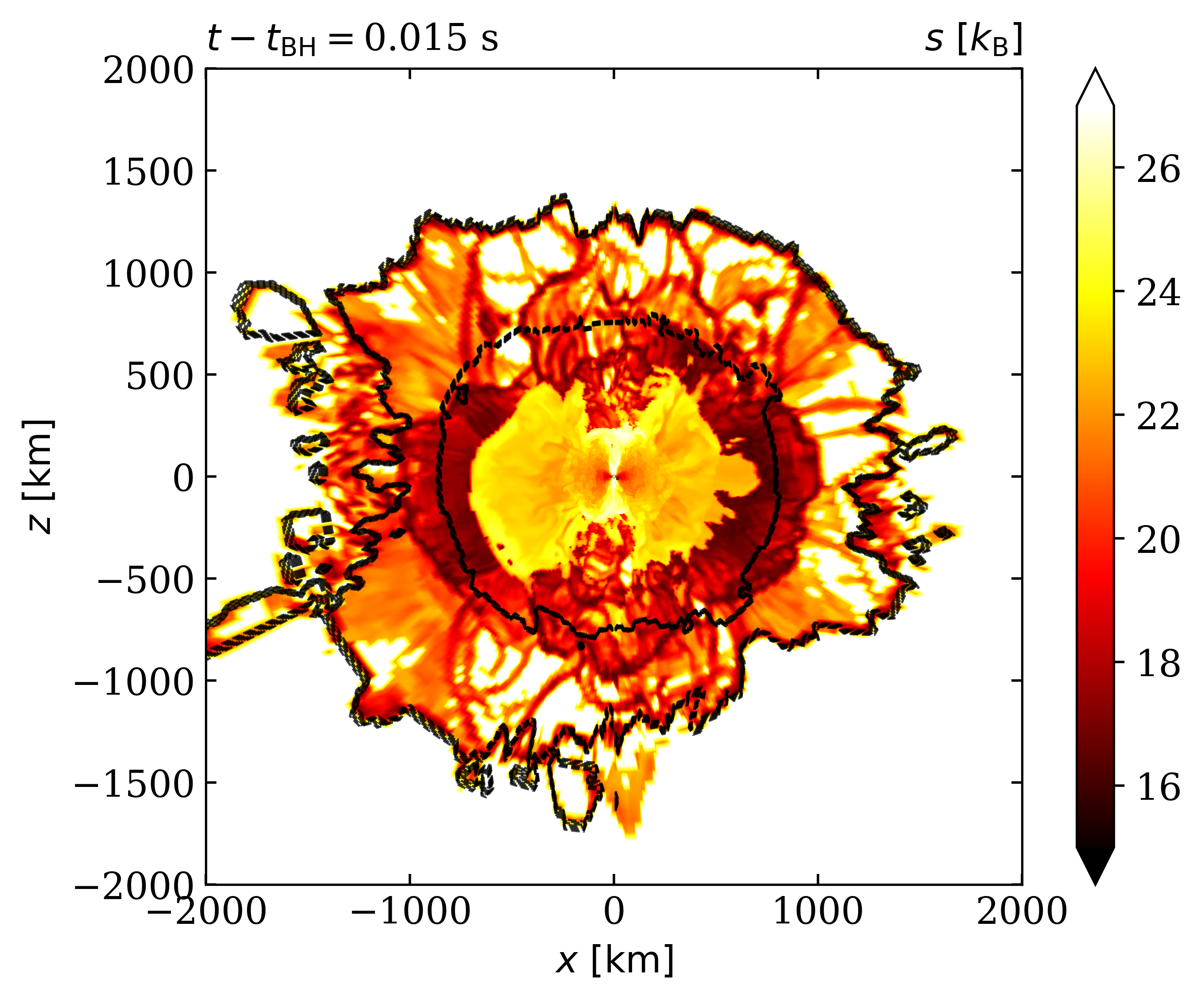
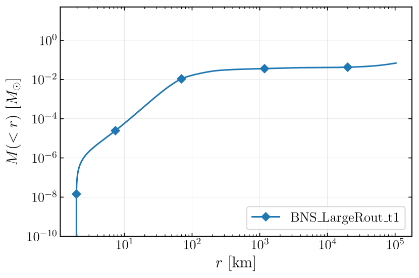
Figure 9: Specific entropy of dynamical ejecta for BNS_LargeRout_t1. Unbound matter with outgoing radial velocity is enclosed within black, dashed curves.

Figure 10: Integrated mass profile (see Eq. 26) for BNS_LargeRout_t1 at the time of hand off. We notice that, even though the domain is large, the integrated mass is dominated by the ejecta; the numerical atmosphere does not contribute significantly.

In addition to the accretion disk, the ID obtained from the HandOff includes the unbound debris from the merger (i.e., the dynamical ejecta). There are two main mechanisms of mass ejection during the merger, tidal interactions and shock heating [see, for instance, Ref. 112]. While the first mechanism predominantly expels cool material from the NSs to the orbital plane of the binary, the second ejects heated material quasiisotropically. In Fig. 10 we visualize the dynamical ejecta for BNS_LargeRout_t1 by plotting the specific entropy, along with dashed lines that contain the ejected material. We identify the ejecta as the parcels of fluid that are unbound, satisfying $(h+b^{2}/\rho)u_{t}<-1$, and move outwards, satisfying $v^{r}>0$. Indeed, we recognize regions with low entropy around the equator, which we associate with the early tidal ejecta, and a quasispherical region with higher entropy, which we associate with the shocked-heated ejecta. We find the total ejecta have a mass of $0.002M_{\odot}$, and an average radial velocity of $0.15c$. These values are consistent with the ranges found in the literature [46, 112, 37], supporting the validity of our methods. Regarding our specific model, the total mass of the ejecta is likely to be overestimated since we do not take neutrino cooling into account and this excess of internal energy increases the amount of unbound material [36]. In Fig. 10 we plot the mass profile

$$M(<r)=\int^{r}\rho\sqrt{-g}\,dV$$ (26)

for the radial extent of the domain and confirm that the enclosed mass in the simulation is dominated by the ejecta– the numerical atmosphere has a negligible contribution, even for such a large domain.

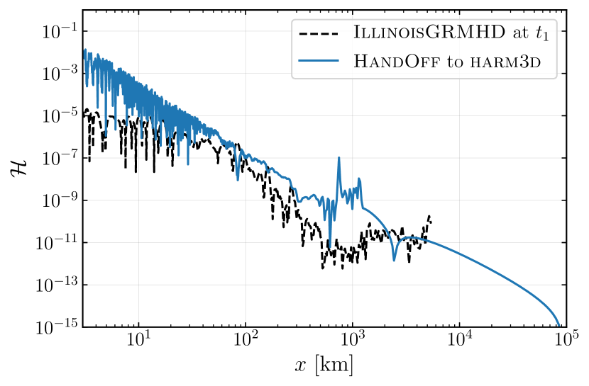
Figure 11: Hamiltonian constraint $\mathcal{H}$ at the $x$-axis at the time of transition for BNS_LargeRout_t1. We plot both the constraints for the evolved metric in IllinoisGRMHD (dashed, black), and for the interpolated/extrapolated metric in Harm3d after the HandOff (solid, blue).

As mentioned, the destination grid of BNS_LargeRout_t1 has its outer boundary much farther away than the original grid of IllinoisGRMHD. Then, as described in Sec. II.7, we need to extrapolate the primitives and spacetime metric. For the “trusted window” in the extrapolation of the spacetime metric, we use $R1=500M_{\odot}$ ($\sim 750\rm{km}$) and $R2=800M_{\odot}$ ($\sim 1200\rm{km}$).

To test the validity of both the interpolated and extrapolated geometry, in Fig. 11 we plot the Hamiltonian constraint along the $x$-axis for IllinoisGRMHD at the time of transition, and for Harm3d after the HandOff. For the latter, we neglect the contribution of matter and assume the spacetime is static. In the extrapolated region, we find the values of $\mathcal{H}$ to be comparable between both codes, although some deterioration in the transition region for Harm3d. In the accretion disk region, we find the values of $\mathcal{H}$ to be comparable between both codes, ensuring the validity of the spacetime metric. However, in the region close to the BH, we find the values of $\mathcal{H}$ to be worst for Harm3d after the HandOff. A similar behavior was found for the momentum constraints. In the following we discuss why this is not a significant concern.

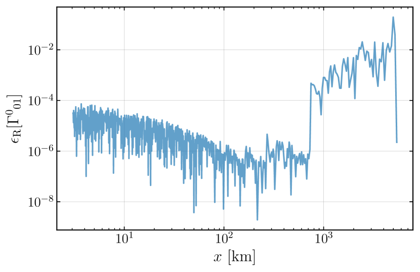
Figure 12: Relative error (see Eq. 15) between the affine connection ${\Gamma^{0}}_{01}$ in IllinoisGRMHD and its values as calculated from the interpolated/extrapolated metric in Harm3d.

Although the spacetime metric is transferred with high-fidelity, we noticed that in regions where the destination grid has higher resolution the interpolant function have regions of size $dx^{\mathrm{IGM}}$ in its domain where the functional form is that of a polynomial, and second order derivatives are not trustworthy. This deteriorates the values of the constraints near the BH. However, only first order derivatives of the spacetime metric play a role in the evolution equations, via the affine connections ${\Gamma^{\lambda}}_{\mu\nu}$. Comparing the relevant connections in IllinoisGRMHD with those recalculated in Harm3d from the interpolated/extrapolated metric, we find they agree with a relative error of order $\sim{}10^{-2}$ or lower in the BH surroundings, ensuring an equivalent gravitational field after the HandOff. As an example of this, in Fig. 12 we plot the relative errors for the case of ${\Gamma^{0}}_{01}$ along the x-axis. Noticeably, the relative errors raise in the region where the numerical metric is replaced by the extrapolated values, but the connections still remain comparable. Indeed, in the next subsection we will show that the evolution of the MHD fields in the extrapolated spacetime has the expected physical behavior, and matches the results from BNS_SmallRout_t1, where extrapolation is not required and the numerical metric is taken directly from interpolation. In particular, we will compare the radial velocity $v^{r}$ of the expanding ejecta of BNS_LargeRout_t1 in the extrapolated region with those results for BNS_SmallRout_t1.

To monitor the degree of axisymmetry of the transitioned spacetime metric we calculate the relative deviations of each local element of volume $\sqrt{-\left|g(r,\theta,\phi)\right|}$ from the corresponding $\phi$-average $\left<\sqrt{-\left|g(r,\theta,\phi)\right|}\right>_{\phi}$ for BNS_LargeRout_t1, and find that:

$$\frac{\left|\sqrt{-\left|g(r,\theta,\phi)\right|}-\left<\sqrt{-\left|g(r,\theta,\phi)\right|}\right>_{\phi}\right|}{\left|\left<\sqrt{-\left|g(r,\theta,\phi)\right|}\right>_{\phi}\right|}<3\times 10^{-3}.$$ (27)

Furthermore, to monitor the degree of stationarity of the transitioned spacetime metric we calculate the relative deviations of each local element of volume for BNS_SmallRout_t0 and BNS_SmallRout_t1 which make use of the same destination grid but transitioned at the different times $t_{0}$ and $t_{1}$, respectively. We find that:

$$\frac{2\left|\sqrt{-\left|g(t_{0},r,\theta,\phi)\right|}-\sqrt{-\left|g(t_{1},r,\theta,\phi)\right|}\right|}{\left|\sqrt{-\left|g(t_{0},r,\theta,\phi)\right|}\right|+\left|\sqrt{-\left|g(t_{1},r,\theta,\phi)\right|}\right|}<2\times 10^{-2}.$$ (28)

In this sense, we argue that the spacetime is approximately axisymmetric and static for the continued evolution in Harm3d.

IV.4 Handing off the postmerger: Continued evolution

We evolve BNS_LargeRout_t1 in Harm3d for $0.1~{}\mathrm{s}$, i.e. up to $0.115~{}\mathrm{s}$ after BH formation. As we describe below, during this period we find the BH accretes $0.023~{}M_{\odot}$ (${\sim}27\%$ of the initial mass of the torus), the accretion rate converges to ${\sim}0.1~{}M_{\odot}s^{-1}$ , the magnetic energy increases by ${\sim}50\%$, and the ejecta expand freely. We do not find significant magnetic outflows from the ergosphere of the remnant. We could have evolved the system for longer, but were limited by computational resources. We used 229 nodes of the the supercomputer Frontera , for approximately 5 days, implying a system usage of almost 30k SUs (System Units). Considering that the number of cells is $1024\times 200\times 400$ (see Appendix A), and that each node has $56$ processors, our code runs at a pace of almost 70k cell updates per second per processor. For consistency checks, we also evolve BNS_SmallRout_t0 and BNS_SmallRout_t1 for approximately $0.04~{}\mathrm{s}$.

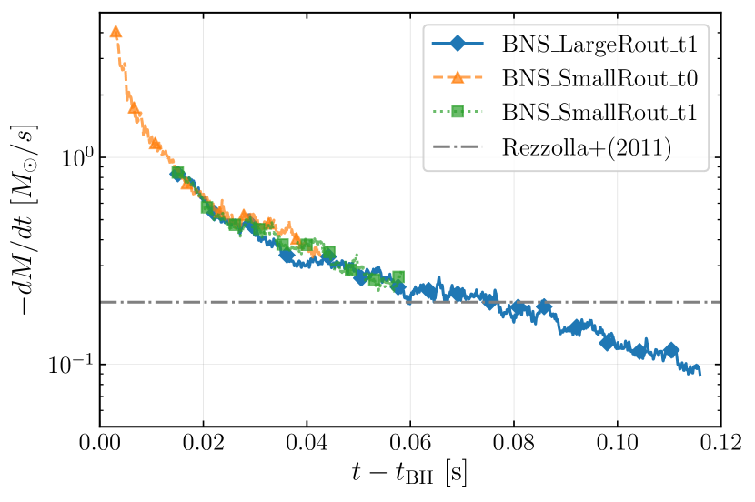
Figure 13: Accretion rate at the horizon for the BNS postmerger simulations, and the reference value of [58]. In every case, the transition is continuous, proving the robustness of the HandOff.

In Fig. 13 we plot the accretion rate at the horizon (${\sim}2.65~{}\mathrm{km}$) for BNS_SmallRout_t0, BNS_SmallRout_t1 and BNS_LargeRout_t1. The plot demonstrates the robustness of the HandOff in the following senses. First, the initial values of the accretion rate for the later transitions at $t_{1}$, BNS_SmallRout_t1 and BNS_LargeRout_t1, match the accretion rate of BNS_SmallRout_t0 at time $t_{1}$, proving both that the HandOff does not introduce unphysical transients and that the evolution of BNS_SmallRout_t0 follows the continuing run in IllinoisGRMHD. Second, the plot shows that the extrapolation of primitives and spacetime metric for BNS_LargeRout_t1 does not lead to unphysical results but matches the results from runs where extrapolation was not needed. Third, the accretion rate approximates to the reference value ${\sim}0.2~{}M_{\odot}s^{-1}$ [58].

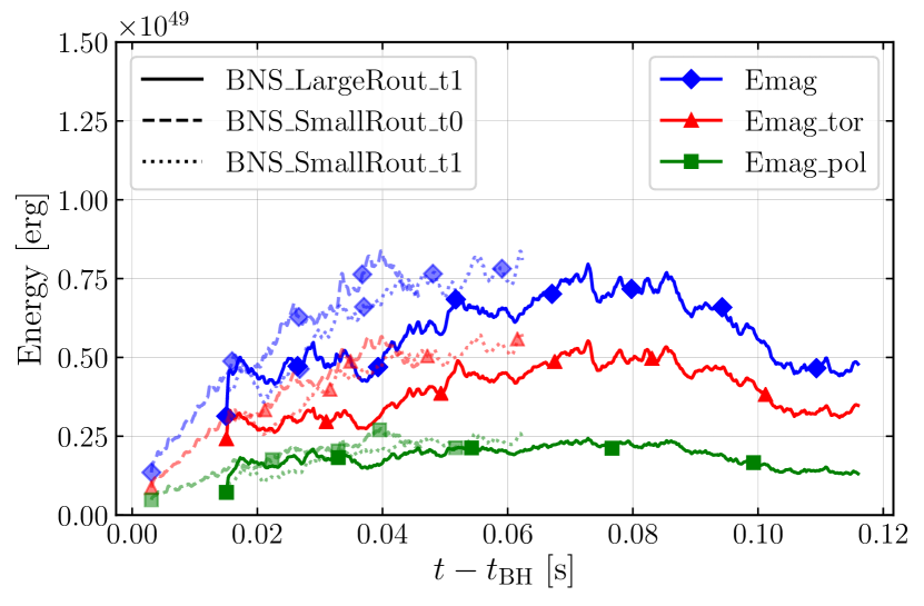
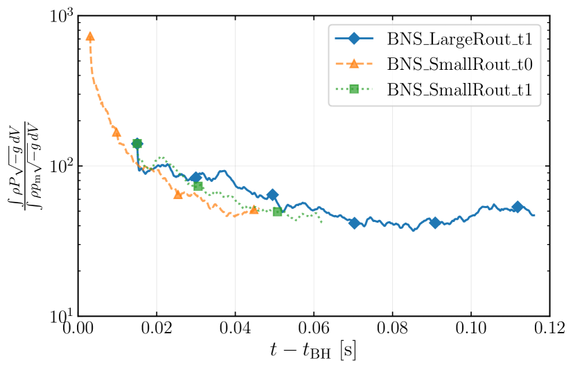
Figure 14: Top: Magnetic energy of BNS postmerger runs (blue), decomposed into toroidal (red) and poloidal (green) components. Bottom: Ratio of the $\rho$-weighted integrals of thermal and magnetic pressure, as a measure of the magnetization of the disk for BNS postmerger runs.

In Fig. 14 (top) we plot the evolution of the magnetic energy for our postmerger simulations, decomposed into toroidal and poloidal components (see Eqs. 23-25), integrated out of the BH horizon. For our fiducial run, BNS_LargeRout_t1, we find $E_{\mathrm{mag}}~{}\sim~{}10^{49}~{}\mathrm{erg}$, with a dominant toroidal component. Our results in this respect are not comparable with the reference simulations of Refs. [58] or [66], because their initial magnetic field was weaker than ours by three orders of magnitude. Instead, we consider the simulation H4B15d150 of Ref. [61], that has an initial field of similar strength, makes use of comparable resolution during the merger, and, though it uses a different EOS, the HMNS collapses to a BH rather promptly. With respect to this simulation, we find a consistent order of magnitude for $E_{\mathrm{mag}}$. Further, the dominance of the toroidal component after merger is a well-known result from the literature [see, for instance, Ref. 66]. From these results, we conclude the HandOff captures the correct strength and topology of the magnetic field after merger. In Appendix C we present resolution diagnostics that demonstrate that the MRI is properly resolved during our runs.

To better understand the effect of transitioning between codes on the magnetization of the disk, in Fig. 14 (top) we also plot the curves for the earlier transition BNS_SmallRout_t0, and for BNS_SmallRout_t1. For every simulation, we notice the magnetic energy grows initially, as expected from magnetic winding and the MRI, but we notice that the curves for the later transitions, BNS_SmallRout_t1 and BNS_LargeRout_t1, do not match the curves of BNS_SmallRout_t0 at $t_{1}$. Instead, the later transitions are initialized to a lower value than BNS_SmallRout_t0 at $t_{1}$, indicating that the magnetic growth is faster in Harm3d than in IllinoisGRMHD, plausibly because the grid of the former has higher resolution and spherical topology, better resolving the magnetic winding effects and the MRI. In fact, we notice that the magnetic energy of the later transitions have a very steep initial growth, until they catch up with the evolved values in BNS_SmallRout_t0.

To measure the dynamical relevance of the magnetic field in the disk, in Fig. 14 (bottom) we plot the evolution of the ratio of the $\rho$-weighted integrals of thermal and magnetic pressure (see Eq. (21)). We find that the dynamical relevance of the field grows in time, until saturation at ${\sim}50$. As a comparison, the FM evolved in the last section, has ${\sim}30$ for this ratio, at $t=9000M$.

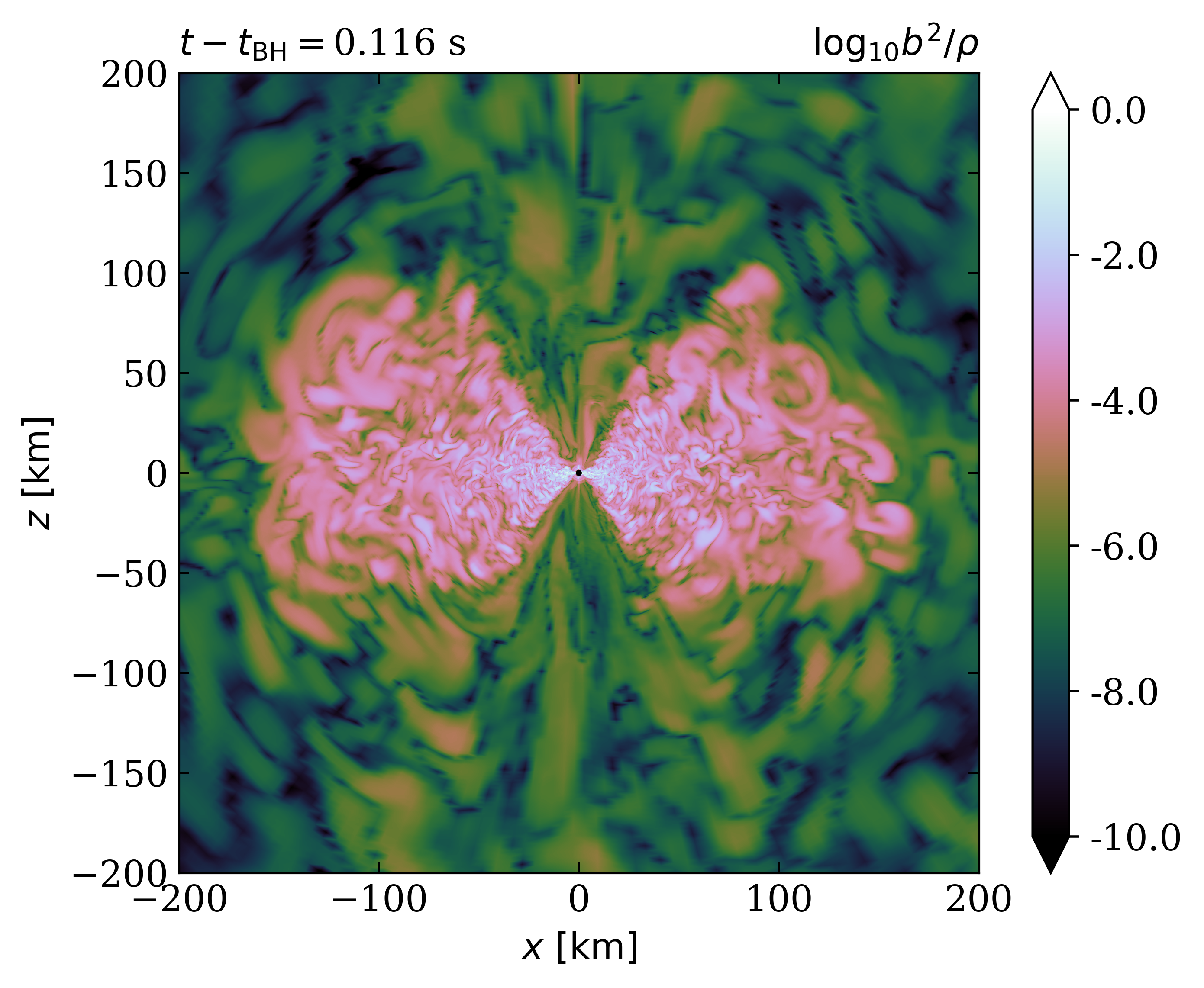
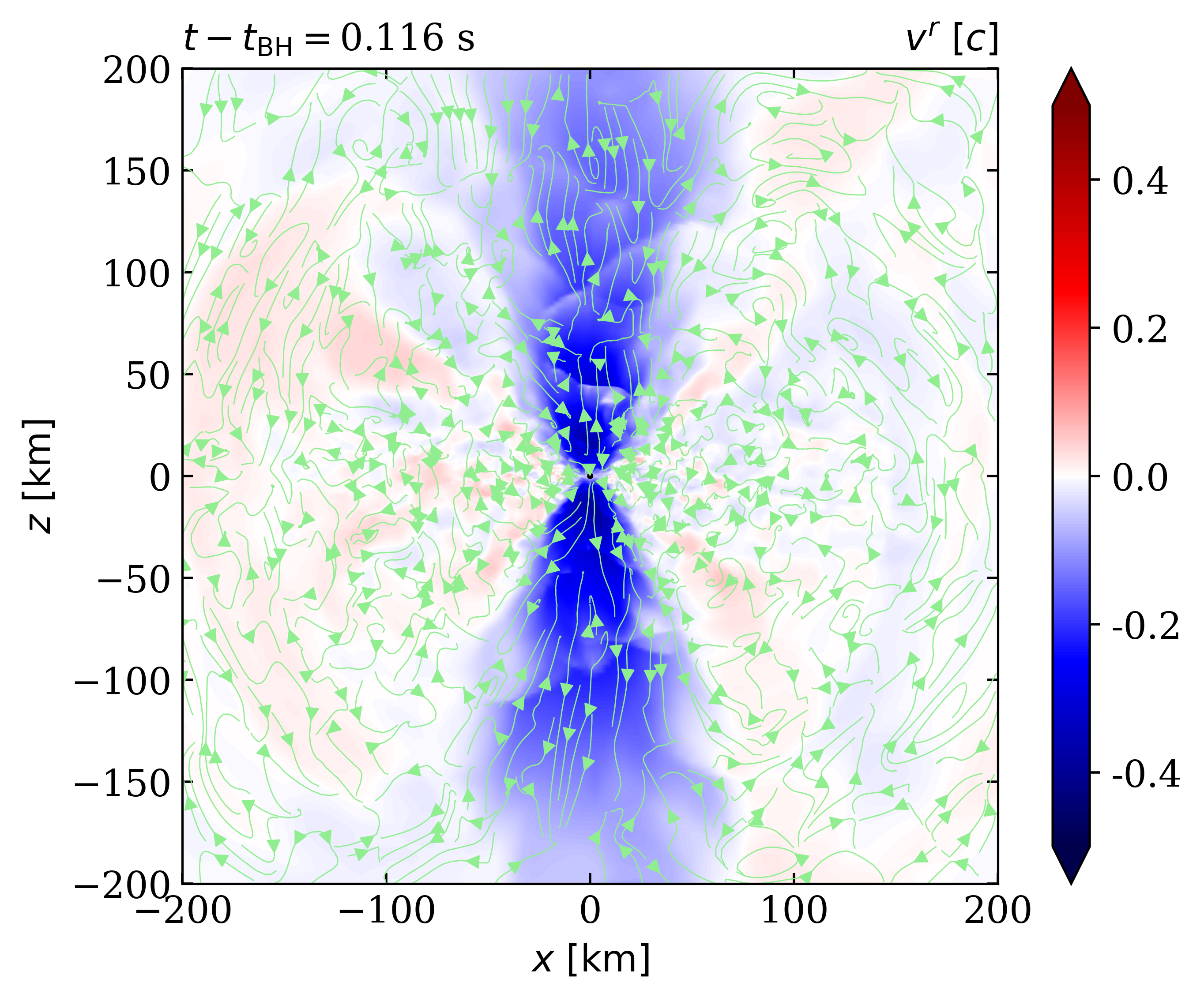
Figure 15: Left: Magnetization $b^{2}/\rho$ at the end of BNS_LargeRout_t1. We notice that, although the disk is fairly magnetized, the funnel is not magnetically dominated. Right: Radial velocity $v^{r}$ and magnetic field lines (green) at the end of BNS_LargeRout_t1. We notice the absence of outflows at the funnel, and that magnetic field lines are poorly ordered.

In Fig. 15 we show a poloidal plot of the magnetization $b^{2}/\rho$ (left), and of the radial velocity of the fluid (right) with magnetic field lines (green arrows), at the end of our fiducial run. Although the magnetization of the disk and the spin of the BH are rather high, we notice that the material in the funnel is not magnetically dominated and a jet has not developed. This is in agreement with results from [66]. Several reasons might help to explain the absence of magnetic outflows: accretion of predominantly toroidal fields disfavours the formation of large-scale magnetic fields at the funnel and its subsequent amplification [see, for instance, 114, 115, 116]; while a long-lived NS remnant can build a strong helical field at the funnel, prompt collapse prevents this scenario [72, 74]; we ignore the drag from neutrino winds, which might help lower the degree of baryon pollution in the polar regions [117]. Still, in Fig. 15 (right) we notice a moderate ordering of the magnetic field lines at the funnel, plausibly stretched by the inflowing material. A mildly relativistic jet might arise in the longer-term [see 74, and refs. therein]. While the magnetic outflows are supressed, Fig. 15 (right) shows outgoing parcels of fluid, or winds, at the boundary of the funnel and the disk [114].

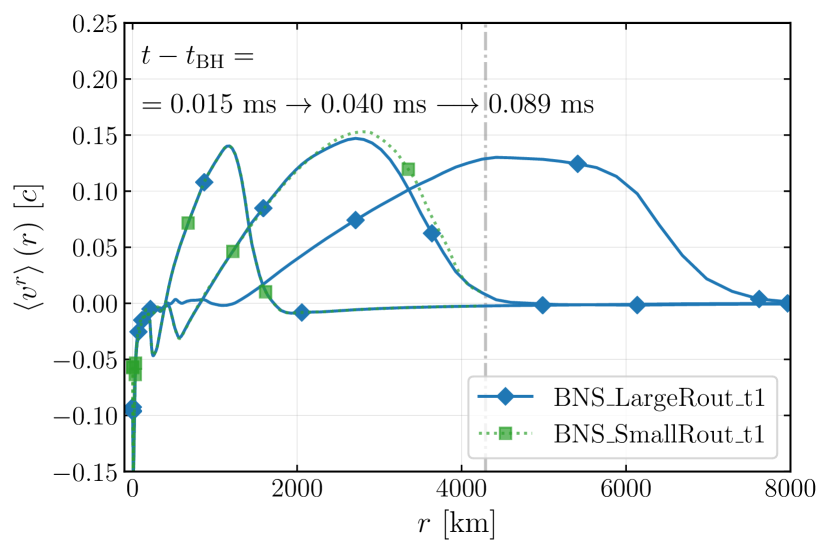
Figure 16: Radial velocity of the ejecta, averaged in $\theta$ and $\phi$, at three different times $t-t_{\mathrm{BH}}=0.015,\,0.04,\,0.089\,\mathrm{ms}$ (left to right). The gray,dotted-dashed line represents the outer boundary of BNS_SmallRout_t1. We notice that the ejecta expand freely through the domain, indicating that the numerical atmosphere and extrapolated metric (BNS_LargeRout_t1) introduced in the HandOff are physically valid. The qualitative agreement between the curves of BNS_SmallRout_t1 and BNS_LargeRout_t1 reflects the near equivalence between the interpolated numerical metric and extrapolated metric.

Finally, we demonstrate the physical validity of the extrapolated metric. In Fig. 16 we plot the radial velocity $v^{r}$ for BNS_LargeRout_t1 and BNS_SmallRout_t1, averaged in $\theta$ and $\phi$:

$$\left\langle v^{r}\right\rangle(r)=\frac{\int v^{r}\sqrt{-g}\,d\theta\,d\phi}{\int\sqrt{-g}\,d\theta\,d\phi}.$$ (29)

We plot $\left\langle v^{r}\right\rangle(r)$ far from the BH, at the boundary of the ejecta with the numerical atmosphere, at three different times: $t-t_{\mathrm{BH}}=0.015,\,0.04,\,0.089\,\mathrm{s}$ (left to right). The dotted-dashed line in Fig. 16 represents the outer boundary of BNS_SmallRout_t1 ($\sim 4300\ \mathrm{km}$). First, we notice that in both runs the ejecta expand freely through the domain, showing the continuity of the handed-off transition. Next, we notice the curves for BNS_LargeRout_t1 and BNS_SmallRout_t1 at $t-t_{\mathrm{BH}}=0.015,\,0.04\,\mathrm{s}$ are qualitatively the same. Since BNS_LargeRout_t1 makes use of the extrapolated metric, and BNS_SmallRout_t1 makes use of the interpolated numerical metric, we conclude these metrics are physically equivalent. We include a later curve for BNS_LargeRout_t1 at $t-t_{\mathrm{BH}}=0.089\,\mathrm{s}$ to show that the HandOff allows for the expansion of the ejecta even further out than the outer boundary of the merger simulation ($\sim 5700\ \mathrm{km}$). We do not include this curve for BNS_SmallRout_t1 because we did not evolve this run for long enough.

V Discussion

The key motivations behind the HandOff package are the advantages of using spherical coordinates over Cartesian to model azimuthal flows. In this article, we argued that spherical coordinates are preferable regarding both physical precision and computational performance. In this section, we provide proof and discussion around such motives.

V.1 Numerical dissipation

In the lore of numerical simulations of fluid dynamics there is a general conviction that momentum is evolved with higher precision if it is aligned with the direction of coordinate lines [for similar comments, see 118, 119, 120, 78]. On the contrary, if the fluid momentum crosses the coordinate faces obliquely, it will be subject to severer numerical errors. In this sense, simulations where linear momentum is most relevant are preferably simulated using Cartesian coordinates, but those that care on angular momentum conservation and transport are preferably simulated using coordinates with spherical topology. These numerical errors usually fall under the name of numerical dissipation—not to be confused with explicit numerical dissipation schemes that damp modes in the solution with wavelengths equal to the grid spacing [121]— and avoiding them in the case of postmerger accretion disks is one of the main motivations behind the HandOff.

A general proof and measure of this phenomenon remains elusive, as numerical errors in the fluxes are also affected by the grid resolution, the particular physical processes involved, and the numerical methods adopted. At the same time, fiducial exact solutions to turbulent MHD are scarce. Numerical experiments that capture the effects of numerical dissipation are usually limited to equilibrium solutions with spacetime symmetries, where some component of the momentum is to be conserved. For the case of a rotating star or an orbiting torus around a BH, one of the causes of Cartesian numerical dissipation has proven to be the poor choice of the coordinate vector base for the momentum decomposition; the best choice being a vector base aligned with the conserved component $l_{\phi}$, like spherical coordinates. This simplifies the source terms in the evolution equations, and reduces the propagation of numerical errors [118, 119, 120]. Plausibly there are other causes behind the Cartesian numerical dissipation in azimuthal flows, like truncation errors introduced when interpolating from the coarsest to finest grid at AMR boundaries. In this section we provide further numerical experiment to demonstrate the effects of Cartesian numerical dissipation in an orbiting torus.

V.1.1 Fishbone-Moncrief disk in hydrostatic equilibrium

Hydrodynamical Fishbone-Moncrief Test

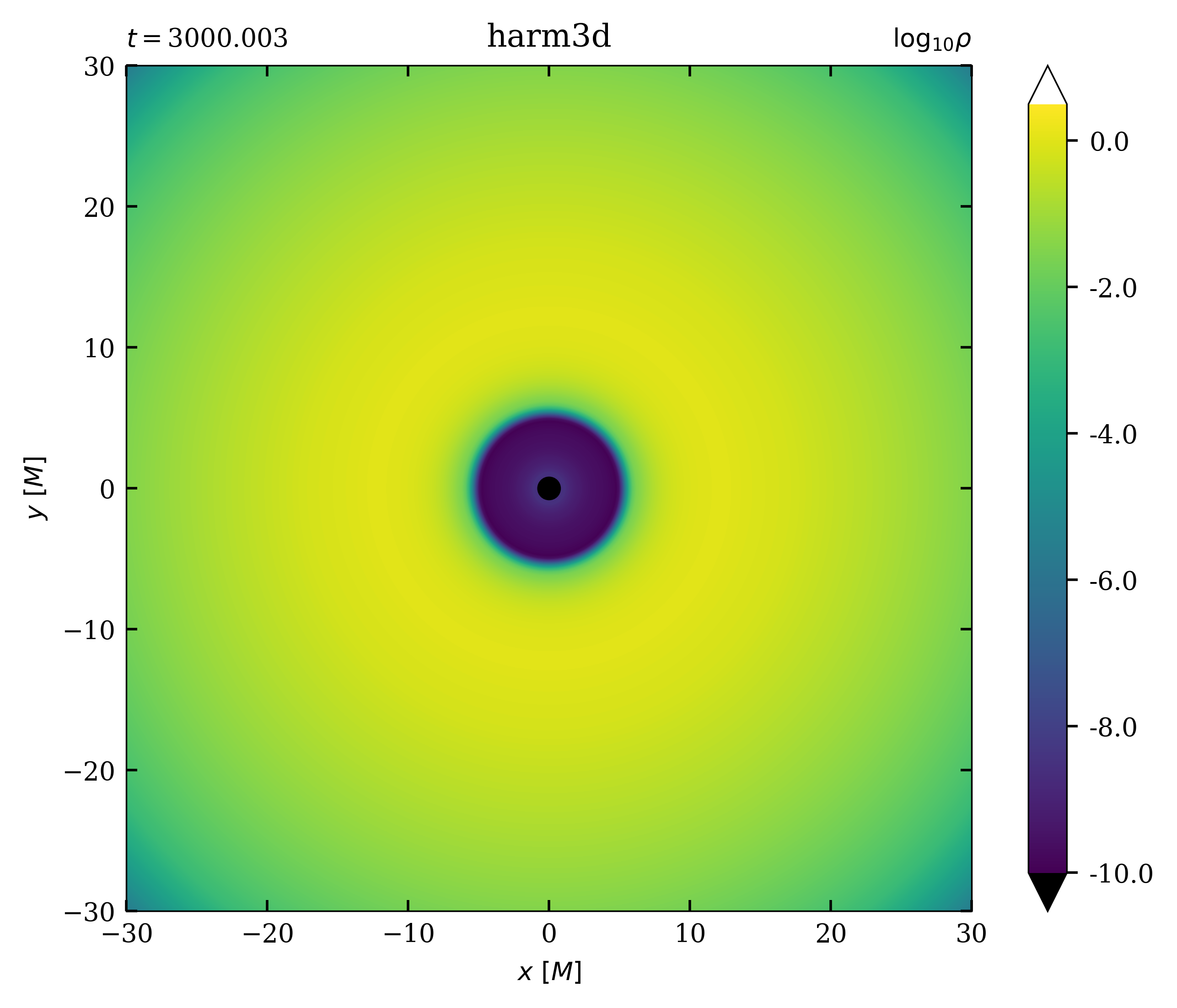
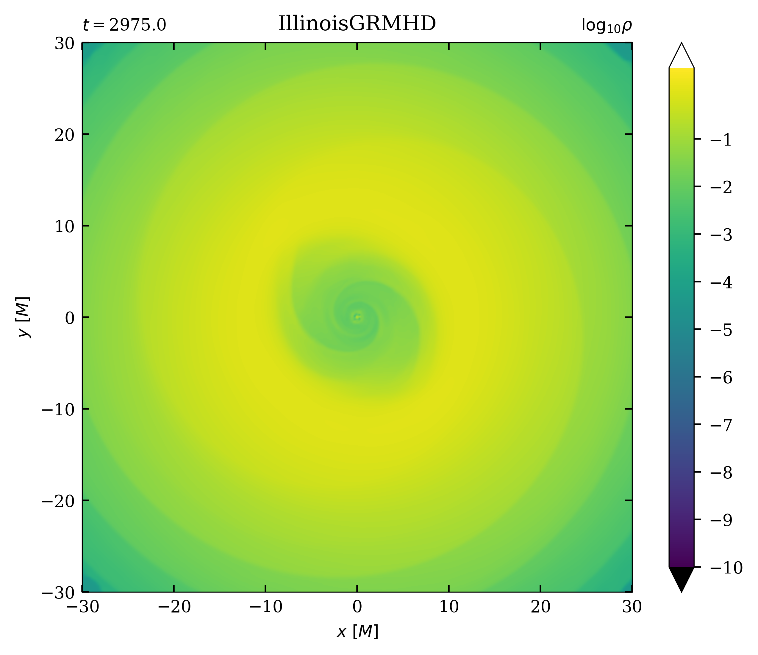
Figure 17: Rest-mass density $\rho$ at equatorial plane for hydrodynamical FM tests in Harm3d (left) and IllinoisGRMHD (right), at time $t\sim{}3000M$. As a consequence of Cartesian numerical dissipation, IllinoisGRMHD fails to maintain the initial hydrostatic equilibrium of the torus.

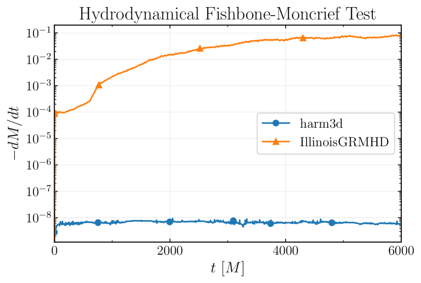
Figure 18: Accretion rate at the BH horizon as a function of time for hydrodynamical FM tests in Harm3d (blue, circle) and IllinoisGRMHD (orange, triangle). Being the formal solution $-dM/dt=0$, we notice that Harm3d with a spherical grid performs better than IllinoisGRMHD by 7 orders of magnitude.

Following Sec. III, we initialize a FM disk in both Harm3d and IllinoisGRMHD, with the same coordinate systems described in such Section. Here, however, we nullify the initial magnetic field and the initial perturbations to the gas pressure, so the ID is in hydrostatic equilibrium. We evolve the system with both codes for $6000M$ in time, and proceed to analyze the deviations from equilibrium as a measure of numerical dissipation.

In Fig. 17 we plot the density around the inner edge of the disk at the equatorial plane in both Harm3d (left) and IllinoisGRMHD (right) at $t=3000M$. We notice that Harm3d manages to maintain the initial cylindrical symmetry of the torus, but IllinoisGRMHD breaks the symmetry of the system developing spiral waves and angular momentum transport that causes accretion. Pressure-supported tori with constant specific angular momentum and entropy are unstable to nonaxisymmetric instabilities [see, for instance, 122] and Cartesian numerical dissipation seems to be triggering those. To better quantify the physical relevance of such instability, in Fig. 18 we plot the accretion rate through the BH horizon in each case. Since the analytical expectation is zero, we notice that Harm3d performs better than IllinoisGRMHD by seven orders of magnitude.

V.1.2 Magnetized Fishbone-Moncrief disk

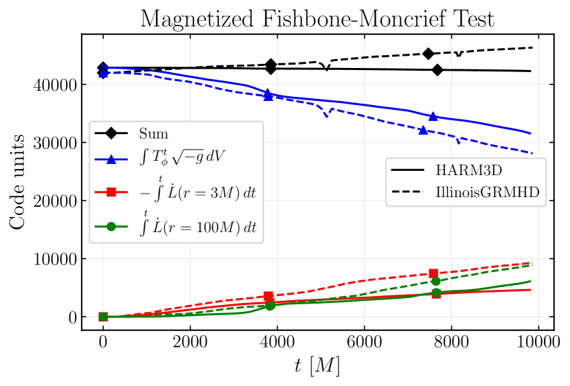
Figure 19: Angular momentum conservation as a function of time for a magnetized FM test in Harm3d (solid, black, diamond) and IllinoisGRMHD (dashed, black, diamond)– the other curves represent the different terms in Eq. (30). While Harm3d manages to conserve angular momentum by $1\%$ with a spherical grid, Cartesian coordinates with block-structured AMR in IllinoisGRMHD conserves angular momentum within $\%10$.

We showed that the effects of Cartesian numerical dissipation are drastic in the case of an orbiting torus in hydrostatic equilibrium. The generalization of this result to more general turbulent MHD flows, however, has its caveats. Indeed, in Sec. III we demonstrated that Cartesian coordinates with AMR can give qualitatively equivalent results than spherical coordinates for the case of a magnetized torus—although still inefficiently since the number of Cartesian cells was more than 80 times larger than of its spherical counterpart. Magnetic-induced turbulence break the laminarity of the azimuthal flow and lessen the numerical convenience of using a spherical grid. But still, a more in-depth analysis will show the superiority of spherical coordinates in modeling azimuthal flows.

In the magnetized FM evolved in Sec. III, given that the spacetime is isometric along the vector field $\partial_{\phi}$, the angular momentum of the plasma $\int T^{t}_{\mu}\partial^{\mu}_{\phi}\sqrt{-g}\,dV$ should be conserved. However, in these simulations, we lfose track of some angular momenta, as parcels of the plasma are accreted by the BH or expelled out of the outer boundary. We expect the following quantity to be conserved instead:

$$\begin{split}\Delta L(t)&=\int_{3M<r<100M}T^{t}_{\phi}\sqrt{-g}\,dV+\\ &+\int^{t}\dot{L}(r=3M)\,dt+\int^{t}\dot{L}(r=100M)\,dt,\end{split}$$ (30)

where the first term contains the angular momentum in the region $3M<r<100M$, and the second and third terms track the loss of angular through the boundaries $r=3M$ and $r=100M$, being $\dot{L}(r)$ the radial angular momentum flux:

$$\dot{L}(r)=\int-T^{r}_{\phi}\sqrt{-g}\,d\theta\,d\phi.$$ (31)

In Fig. 19 we plot these terms and their sum for both codes, Harm3d and IllinoisGRMHD. We find that Harm3d conserves angular momentum by $1\%$ but IllinoisGRMHD by $10\%$, demonstrating the higher fidelity of spherical coordinates in capturing the angular momentum conservation and transport.

V.2 Computational performance

There are many reasons why using Harm3d instead of IllinoisGRMHD for the postmerger evolution is computationally convenient: Flexible coordinate systems with spherical topology can sample the domain optimally and, for instance, do not over-resolve the angular coordinates at large distances like AMR-structured Cartesian coordinates. The absence of AMR boundaries in Harm3d reduces the number of buffer regions, improving memory usage and scaling. Freezing the spacetime evolution after spacetime equilibration significantly lessen the computational workload. For azimuthal flows, fewer numerical cells are required in spherical coordinates to capture the relevant physical processes (a factor of $\sim{}80$ for the FM test in Sec. III). The infrastructure around Harm3d is highly optimized and lightened for accretion disk simulations.

To demonstrate the computational efficiency of Harm3d, we compare the performance of IllinoisGRMHD when evolving the spacetime and matter fields of a stable neutron star, with the performance of Harm3d when evolving a magnetized torus in a static spacetime for a rotating BH. We submit both tests in a unigrid with $64^{3}$ cells, and make use of a single computational process. We find that IllinoisGRMHD performs $37,000$ cell updates per second per processor and Harm3d outperforms this by more than $\times 10$, performing $415,000$ cell updates per second per processor .

VI Summary and conclusions

We presented the tools to transition a GRMHD simulation between two numerical codes, IllinoisGRMHD and Harm3d, that make use of numerical grids with different resolutions and topologies. Moreover, we presented techniques to extrapolate the spacetime metric and MHD primitives to arbitrarily large radii, allowing us to extend the numerical domain of the destination grid. This set of methods, enclosed under the name of the HandOff, are particularly interesting for transitioning the outcomes of BNS or BH-NS mergers to a grid adapted to the geometry and requirements of the postmerger. In Appendix A we give the implementation details of this grid.

We validated the HandOff with the well-known case of a magnetized torus around a rotating BH. We applied the HandOff at different stages of the accretion process and confirmed the package successfully captures the state of the plasma and spacetime metric and transforms them to a general grid.

We applied the HandOff to a BNS postmerger, after the BH had formed. We modeled matter as a magnetized ideal fluid with adiabatic index $\Gamma=2$. To test the reliability of the HandOff, we applied it at different times and to different destination grids. Our fiducial simulation, BNS_LargeRout_t1, starts from ID provided by the HandOff at $t-t_{\mathrm{BH}}=0.015\mathrm{s}$, makes use of the large grid described in Appendix A, and lasts for ${\sim}~{}0.1\mathrm{s}$. Since the destination grid is larger than the initial grid for the merger, we needed to extrapolate the MHD primitives and spacetime metric to the complementary cells. After a careful analysis, we demonstrated our results from the HandOff are independent of the time of transition, and of the destination grid. Furthermore, we showed these results are in agreement with reference simulations in the literature.

In Sec. V.1 we demonstrated that the effects of Cartesian numerical dissipation are drastic for an orbiting torus in hydrostatic equilibrium, and moderate for a highly magnetized and turbulent torus. This implies that long-term simulations of accretion disks in BNS postmergers with block-structured AMR can be spoiled by Cartesian numerical dissipation, particularly in the absence of magnetic fields or even for realistic magnetic fields in the initial stars ($\sim 10^{12}\mathrm{G}$) that lead to mildly magnetized postmerger disks. For this reason, and the significant computational convenience of spherical grids to parameterize large computational domains, we consider that mapping the postmerger to a spherical grid is most convenient.

We conclude the HandOff enables us to perform long-term, highly accurate and coordinate-optimized simulations of BNS postmergers, generating ID from the end of a BNS merger simulation performed in full numerical relativity. Future work will focus on improving our models for the matter fields during the merger, adopting finite-temperature and tabulated EOS and taking neutrino effects into account. Next, we will extend the HandOff to transition these realistic simulations to the modern code HARM3D+NUC [81].

Appendix A Design of postmerger grid

The distorted spherical grid we often use in Harm3d, one that uses a uniform spacing in $\log(r)$ and is concentrated in the poloidal direction near the equator, is not particularly well-suited for long-term evolutions of ejecta launched closer to the equator and relatively narrow jets along the poles. In order to resolve the jet at large distances and keep the number of poloidal cells fixed, we must increase $\Delta\theta$ in the equator and decrease it near the poles as $r$ grows. Using larger $\Delta\theta$ at the smallest radii also allows us to use larger time steps, as they are set by the smallest cell-crossing time of the fastest MHD wave in the domain, which is usually determined by the innermost azimuthal extent at the poles, $\simeq r_{\mathrm{in}}\left(\Delta\theta/2\right)\,\Delta\phi$, where $r_{\mathrm{in}}$ is the innermost radial coordinate on the grid. This means that our conventional grid is adequate at smaller radii, but we must transition to one that is more focused along the poles at larger radii.

Since the goal is to capture the ejected material out to $\mathcal{O}(1\mathrm{s})$ of time or $\mathcal{O}(1~{}\mathrm{light-second})\sim\mathcal{O}(10^{5}GM_{\mathrm{BH}}/c^{2})$ of distance, our typical $\log(r)$ grid would require so many grid points it would be computationally prohibitive. Since the ejected material is expected to be nearly ballistic beyond $r\simeq 10^{3}M_{\mathrm{BH}}$, increasing $\Delta r(r)$ in a hyperexponential way provides an effective solution at covering large distances with fewer cells:

$$\begin{split}r(x^{\tiny\left(1\right)})=&r_{0}+\left(r_{\mathrm{in}}-r_{0}\right)\times\\ &\exp{\left[c_{1}\left(x^{\tiny\left(1\right)}/x_{\mathrm{he}}\right)+c_{2}\left(x^{\tiny\left(1\right)}/x_{\mathrm{he}}\right)^{{n}}\right]}\quad,\end{split}$$ (32)

where the coefficients in the exponent ensure that $r(0)=r_{\mathrm{in}}$, $r(x_{\mathrm{he}})=r_{\mathrm{he}}$, $r(1)=r_{\mathrm{out}}$ ($r_{\mathrm{out}}$ is the outermost radial coordinate):

$$c_{1}=\frac{d_{1}-d_{2}\,x_{\mathrm{he}}^{{n}}}{1-x_{\mathrm{he}}^{{n}-1}}\quad,\quad c_{2}=\frac{d_{2}\,x_{\mathrm{he}}^{{n}}-d_{1}\,x_{\mathrm{he}}^{{n}-1}}{1-x_{\mathrm{he}}^{{n}-1}}\quad,$$ (33)

and

$$d_{1}=\ln{\left(\frac{r_{\mathrm{he}}-r_{\mathrm{in}}}{r_{\mathrm{in}}-r_{0}}\right)}\quad,\quad d_{2}=\ln{\left(\frac{r_{\mathrm{out}}-r_{\mathrm{in}}}{r_{\mathrm{in}}-r_{0}}\right)}\quad.$$ (34)

For the run BNS_LargeRout_t1 we use $n=10$, $r_{0}=0$, $r_{\mathrm{in}}=1.31~{}M_{\odot}$ , $r_{\mathrm{he}}=10^{4}~{}M_{\odot}$, $r_{\mathrm{out}}=7.2\times 10^{4}M_{\odot}$, $dx^{\tiny\left(1\right)}=1/1024$, and $0\leq x^{\tiny\left(1\right)}\leq 1$.

The poloidal discretization joins two regions: an inner one with cells focused near the equator and an outer region with more cells near the poles. The two regions are smoothly and continuously connected through use of a transition function, similar to the strategy used in our “dual fisheye” grids [102]. The poloidal coordinate in terms of the numerical coordinate $x^{\tiny\left(2\right)}$ is:

$$\begin{split}\theta(x^{\tiny\left(2\right)})=&\pi\left\{x^{\tiny\left(2\right)}-a_{2}\left[\mathcal{T}(x^{\tiny\left(2\right)})-\mathcal{T}(1/2)-\right.\right.\\ &\left.\left.-\left(x^{\tiny\left(2\right)}-1/2\right)\left(\mathcal{T}(1)-\mathcal{T}(0)\right)\right]\right\}\quad,\end{split}$$ (35)

where $\mathcal{T}(x)$ is the integral of the approximate boxcar function from [102]:

$$\mathcal{T}(x^{\tiny\left(2\right)})\equiv\frac{1}{2}\left[\Sigma(x^{\tiny\left(2\right)}-1/2+\delta_{2})-\Sigma(x^{\tiny\left(2\right)}-1/2-\delta_{2})\right].$$ (36)

and

$$\Sigma(x)\equiv\frac{1}{h_{2}}\ln\cosh\left(h_{2}\ x\right)\quad.$$ (37)

Here, $h_{2}$ controls the steepness of the transition, and $\delta_{2}$ controls the fraction of cells that are in the equatorial portion of the poloidal grid. We use $h_{2}=20$, $\delta_{2}=0.3$, $dx^{\tiny\left(2\right)}=1/200$, and $0\leq x^{\tiny\left(2\right)}\leq 1$.

The transition between the inner and outer regions is handled by changing the amplitude of the grid distortion, $a_{2}$, with respect to $r$:

$$a_{2}=a_{2}(r)\equiv a_{2\mathrm{1}}f(r,r_{j},h_{j})+\left[1-f(r,r_{j},h_{j})\right]a_{2\mathrm{2}}\quad,$$ (38)

where the transition function is

$$f(r,r_{j},h_{j})\equiv\frac{1}{2}\left\{1+\tanh{\left[h_{j}\left(r-r_{j}\right)\right]}\right\}\quad.$$ (39)

The two amplitudes, $a_{2\mathrm{1}}$ and $a_{2\mathrm{2}}$, are set by different criteria. The amplitude for the inner portion is set so that the spacing near the equator is such that the number of cells per vertical disk scale height, $N_{H/r}$, is equal to the 32 cells recommended to adequately resolve the MRI [124]:

$$a_{2\mathrm{1}}=\frac{1-N_{2}\left(H/r\right)/\left(\pi N_{H/r}\right)}{1-2\delta_{2}}\quad,$$ (40)

where $N_{2}$ is the number of cell extents in the $x^{\tiny\left(2\right)}$ direction. The outer amplitude is set so that the poloidal spacing near the poles follow the parabolic flow contours often found in the jets of GRMHD simulations [125]: $z=R^{n_{1}}$, where $R\equiv r\sin{\theta}$ is the cylindrical radius, and $1<n_{1}\lesssim 2.67$ for general outflows. Using the small angle approximation, $\theta\simeq r^{n_{j}}$, where $n_{j}\equiv\left(1/n_{1}-1\right)$. The funnel wall shape arising in GRMHD simulations with spinning black holes closely follows the curve with $n_{1}\simeq 3/2$ or $n_{j}\simeq-1/3$ [125], and is the value used here. The amplitude, $a_{2\mathrm{2}}$, must vary with radius such that $d\theta_{j}$, the approximately $x^{\tiny\left(2\right)}$-independent spacing local to the jet, follows these contours at $r>r_{j}$, where $r_{j}$ is the radius at which we specify this transition occurs. At $r=r_{j}$, we set $d\theta_{j}$ to be $90\%$ of what it would be if the grid was uniform in $\theta$. The amplitude is finally calculated using this $r$-dependent $d\theta_{j}$:

$$a_{2\mathrm{2}}=-\frac{1-N_{2}d\theta_{j}(r)/\pi}{2\delta_{2}}\quad,$$ (41)

where $d\theta_{j}(r)=\left(0.9\pi/N_{2}\right)\left(r/r_{j}\right)^{n_{j}}$, $n_{j}=-1/3$, and $r_{j}=300M_{\odot}$.

The azimuthal grid spacing for the new grid remains uniform, with $\phi\in\left[0,2\pi\right]$ and $d\phi=2\pi/N_{3}$, where $N_{3}$ is the number of cells in the azimuthal extent.

In Fig. 6 (right) we plot the cell lengths of this grid, as a function of radii and $\theta\in(0,\pi)$. Regarding $\Delta r$, we notice the transition of its slope from exponential to hyperexponential at $r{\sim}10^{3}~{}\mathrm{km}$. Although $\Delta\phi$ is uniform, the cell length $r\sin\theta\Delta\phi$ grows with $r$ because of its explicit radial dependence, and spans different resolutions at a given radius because of the different values of $\theta\in(0,\pi)$. Finally, $r\Delta\theta$ also grows with $r$ because of its explicit radial dependence, and spans different values at a given radius because, as described above, $\Delta\theta$ is not uniform but focuses on the equator at small radii, and on the axis at larger radii. We notice this transition at $r{\sim}10^{3}~{}\mathrm{km}$.

Appendix B Boundary conditions at the axis

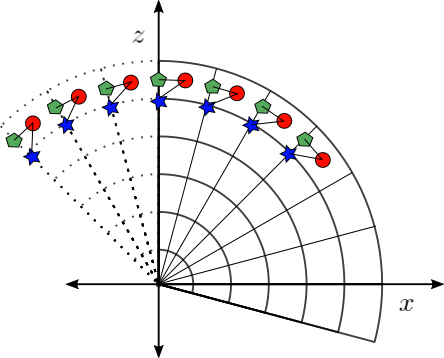
Figure 20: Sketch of grid cells next to the positive $z$-axis. Red circles represent the positions of the cell centers, green polygons represent the position of the lower $\theta$-face of each cell, and blue stars represent the lower corners. Dotted cells represent ghosts cells. The cell center of these ghost cells are mapped to the cell center of physical cells across the axis. The lower faces and corners of the ghost cells, however, are shifted by $+\Delta\theta$ and map to the upper-face of the corresponding physical cells.

Previous simulations of accretion disks in Harm3d excise a portion of the domain around the polar axis [see, for instance, 80, 108, 126]. In these simulations, the polar coordinate $\theta$ is restricted to an interval $(\theta_{\mathrm{c}},\pi-\theta_{\mathrm{c}}$), where $\theta_{\mathrm{c}}>0$ is the extent of the cutout in $\theta$ from the axis. This is convenient for two reasons: First, the coordinate singularity at the axis is excised from the domain. Second, the innermost azimuthal extent at the poles is increased from $r_{\mathrm{in}}\sin(\Delta\theta/2)\Delta\phi$ to $r_{\mathrm{in}}\sin(\theta_{\mathrm{c}}+\Delta\theta/2)\Delta\phi$ and, since the time step in spherical coordinates is restricted to the cell-crossing time of this extent, the time step is increased accordingly. However, cutting out the domain has its drawbacks: The simulation lacks a portion of the the funnel region and therefore of the magnetic outflows, and even the rest of the funnel might be affected by the boundary conditions imposed at the cutout, which are usually reflective or outflow.

These drawbacks are not severe in previous applications, where the funnel is mostly evacuated and the magnetic outflows expand through the numerical atmosphere, but that is not the case for a BNS postmerger. In the latter, the funnel is baryon polluted, with a complex magnetic field structure, and the magnetic outflows propagate through the dynamical ejecta creating a complex jet-cocoon system that eventually breaks-out from the debris. A cutout in $\theta$ would prohibit the appropriate modeling of these phenomena. For this reason, we remove the cutout and implement appropriate boundary conditions at the polar axis, as we describe below.

Formally, the cutout is still present to avoid the coordinate singularity at the axis, but it is reduced to a small value. Specifically, the cell centered coordinates of the cells next to the positive [negative] $z$-axis have coordinates $(r,\Delta\theta/2+\theta_{\mathrm{c}},\phi)$ [$(r,\pi-\Delta\theta/2-\theta_{\mathrm{c}},\phi)$], with $\theta_{\mathrm{c}}\sim 10^{-14}$. The three ghost cells in $\theta$ before [after] these cells are mapped to the physical coordinates across the axis, with cell centered coordinates $(r,\theta_{\mathrm{c}}+j\Delta\theta+\Delta\theta/2+\theta_{\mathrm{c}},\phi+\pi)$ [$(r,\pi-\theta_{\mathrm{c}}-j\Delta\theta-\Delta\theta/2-\theta_{\mathrm{c}},\phi+\pi)$], with $j=0,1,2$. In Fig. 20 we sketch the cell centers of physical and ghost cells (dashed) around the positive $z$-axis with red circles.

Although the cell centers of the ghost cells in $\theta$ match the cell centers of physical cells across the axis, that is not the case for the lower corners and lower $\theta$-faces. The cell-corners and lower $\theta$-faces of the ghost cells are shifted by $+\Delta\theta$, so they stand at a cell length distance from the corresponding cell positions at the boundary. In other words, the lower $\theta$-face of the ghost cells maps to the upper $\theta$-face of the physical cells across the axis. In Fig. 20 we sketch the positions of the lower $\theta$-faces for ghosts (dashed) and physical cells with green polygons, and the corners with blue stars. This is important, for instance, when calculating finite differences across the axis for the spacetime connections, or for the curl of $A_{\mu}$.

Having set the coordinates of the ghost cells in $\theta$, we evaluate the spacetime metric at these cells, and multiply its components $g_{\mu\nu}$ by parity factors that ensure continuity across the axis. In particular, we follow Refs. [78] (see Table 1 of that reference) and change the sign of $g_{t\theta},g_{r\theta},g_{\phi\theta}$ and their symmetric permutations. The metric component $g_{\phi\phi}$ tends to zero towards the axis, so we enforce $g_{\phi\phi}=1\times 10^{-14}$ if this component takes a smaller value at the $\theta$-face and corners of the physical cells next to the axis. We fill the ghost cells with MHD primitives from the matching physical cells, and take parity factors into account by changing the sign of the tensor components $B^{\theta},v^{\theta}$ [78]. We use the geometry and primitives in these ghost regions as boundary conditions to evolve the conserved variables in the physical cells next to the axis. Subsequently, the MHD primitives in the ghost cells are updated after each time step with the evolved values at the matching physical cells, and multiplied by the corresponding parity factors.

The evolution of the magnetic field requires further care. In the FluxCT algorithm [89], the electric field $\mathbf{E}$ is calculated at the cell-edges, and the extent or definition of those edges is singular for cells next to the axis. As first described by Refs. [127] (see the supplemental material of that reference), we find that a nonzero value of $E_{\phi}$ at the axis gives raise to an artificial growth of the magnetic flux in the radial direction. We apply the same techniques of Ref. [127] to circumvent this problem. Since the extent of the cell-edge in $\phi$ is zero at the axis, we set the electric field component $E_{\phi}$ to zero in those cells. Further, since the cell-edge in $r$ is the same for every cell around the axis at a given height $z$, we set $E_{r}$ to a unique value in these cells. This value results from the $\phi$-average of $E_{r}$ around the axis at height $z$.

Appendix C Resolution Diagnostics

In this appendix we calculate resolution diagnostics to demonstrate the convergence of the MRI-driven turbulence in the postmerger disk. We follow the analyses of Refs. [128, 108, 129, 76].

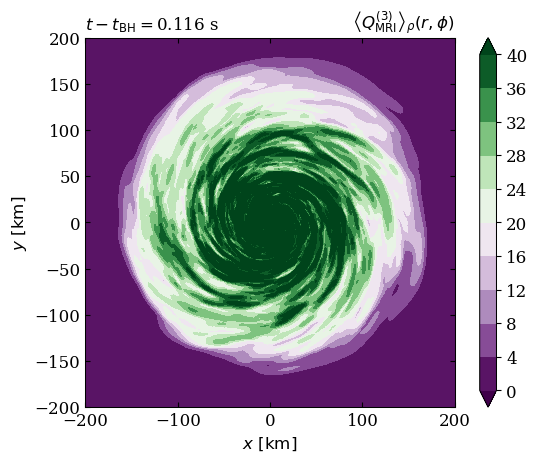
Figure 21: Quality factors of MRI resolution, weighted by $\rho$ and averaged in $\theta$. We emphasize they satisfy $\left\langle Q^{(2)}\right\rangle_{\rho}>10$ (left) and $\left\langle Q^{(3)}\right\rangle_{\rho}>20$ (right), adequately resolving the MRI wavelength.

We start by calculating the number of cells within the linear MRI wavelength, or quality factors:

$$Q^{(i)}=\frac{2\pi\left|b^{(i)}\right|}{\Delta x^{(i)}\Omega_{\mathrm{K}}(r)\sqrt{\rho h+2p_{\mathrm{m}}}}.$$ (42)

We multiply the latter by $\rho$ to focus on the disk, and average over the polar direction:

$$\left\langle Q^{(i)}\right\rangle_{\rho}(r,\phi)=\frac{\int_{0}^{1}Q^{(i)}\rho\sqrt{g^{\prime}}\,dx^{(2)}}{\int_{0}^{1}\rho\sqrt{g^{\prime}}\,dx^{(2)}}.$$ (43)

In Fig. 21 we plot these quantities at the end of BNS_LargeRout_t1, and notice they satisfy $\left\langle Q^{(2)}\right\rangle_{\rho}>10$ and $\left\langle Q^{(3)}\right\rangle_{\rho}>20$, the conditions for converged MRI behavior from resolution studies.

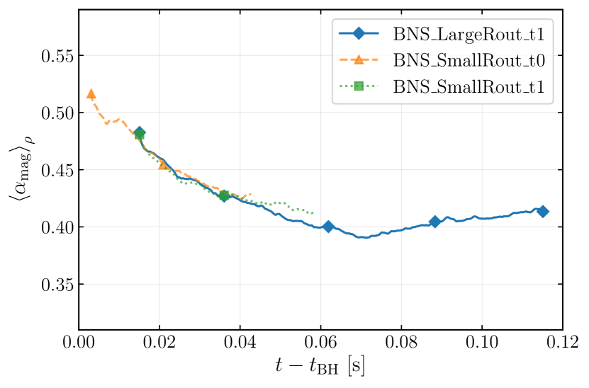
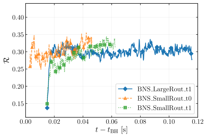
Figure 22: Nonlinear diagnostics of MRI resolution $\alpha_{\mathrm{mag}}$ (left) and $\mathcal{R}$ (right) (see Eqs. 44 and 45). They converge to $\sim 0.4$ and $\sim 0.3$, respectively, implying proper resolution of the MRI modes [128, 129].

We also calculate nonlinear diagnostics: The weighted ratio of the Maxwell stress to the magnetic pressure

$$\left<\alpha_{\mathrm{mag}}\right>_{\rho}=\frac{\int\alpha_{\mathrm{mag}}\rho\sqrt{g}\,dV}{\int\rho\sqrt{g}\,dV},\ \ \alpha_{\mathrm{mag}}=\frac{2\sqrt{b_{r}b^{r}}\sqrt{b_{\phi}b^{\phi}}}{b^{2}},$$ (44)

and the weighted ratio of energies between these components

$$\mathcal{R}=\frac{\int B_{r}B^{r}\rho\sqrt{-g}\,dV}{\int B_{\phi}B^{\phi}\rho\sqrt{-g}\,dV}.$$ (45)

In Fig. 22 we plot these quantities as a function of time. We find $\alpha_{\mathrm{mag}}$ becomes approximately constant, as expected from the correlation induced on $b^{r}$ and $b^{\phi}$ by the MRI, and converges to $\sim 0.4$, the saturation value of shearing-box simulations of Ref. [128]. On the other hand, we find $\mathcal{R}\sim 0.3>0.2$, satisfying the criteria of Ref. [129]. From this plot we also notice that the later transitions, BNS_SmallRout_t1 and BNS_LargeRout_t1, are initialized to a smaller value than BNS_SmallRout_t0 at such time, and then they rapidly catch up with the convergent value. This suggests the MRI was not properly resolved in IllinoisGRMHD, proving the need for the transition to a higher-resolution grid. We conclude the MRI is well resolved in the run BNS_LargeRout_t1 that makes use of the grid described in Appendix A.

Appendix D Magnetic field decomposition

Along this article, we decomposed the magnetic field in the direction of the fluid velocity $\tilde{v}^{i}$ and its orthogonal frame, and interpreted these as toroidal and poloidal components of the field, respectively (see Eqs. 23-25). This interpretation is supported by the reduction of this decomposition to poloidal-toroidal in the case of axisymmetric axial flows, and by Ref. [111] that successfully applied this decomposition and interpretation to rotating NSs. In this Appendix we demonstrate that such decomposition and interpretation are also valid for the case of magnetized accretion disks.

We decompose the magnetic field in terms of the poloidal coordinate vector $\phi^{i}$:

$$B^{i}=B_{\mathrm{tor}}\phi^{i}+B_{\mathrm{pol}}^{i},$$ (46)

where

$$\phi^{i}=\left[0,0,\frac{1}{\sqrt{g_{\phi\phi}}}\right],$$ (47)

$$B_{\mathrm{tor}}=B^{i}\phi_{i}.$$ (48)

It can be proved that the magnetic energy (Eq. 23) takes the form:

$$E_{\mathrm{mag}}=E^{\phi-\mathrm{tor}}_{\mathrm{mag}}+E^{\phi-\mathrm{pol}}_{\mathrm{mag}}+E^{\mathrm{\times}}_{\mathrm{mag}},$$ (49)

where

$$E^{\phi-\mathrm{pol}}_{\mathrm{mag}}=\frac{1}{2}\left[B^{2}_{\mathrm{pol}}\left(1+\tilde{v}^{2}\right)-\left(B^{i}_{\mathrm{pol}}\tilde{v}_{i}\right)^{2}\right],$$ (50)

$$E^{\phi-\mathrm{tor}}_{\mathrm{mag}}=\frac{1}{2}\left[B_{\mathrm{tor}}^{2}\left(1+\tilde{v}^{2}-\frac{\tilde{v}_{\phi}\tilde{v}_{\phi}}{\left|g_{\phi\phi}\right|}\right)\right],$$ (51)

$$E^{\mathrm{\times}}_{\mathrm{mag}}=-\left(B^{i}_{\mathrm{pol}}\tilde{v}_{i}\right)B_{\mathrm{tor}}\frac{\tilde{v}_{\phi}}{\sqrt{g_{\phi\phi}}}.$$ (52)

As we can see from the latter expressions, the decomposition in terms of the coordinate vector $\phi^{i}$ includes a cross term $E^{\mathrm{\times}}_{\mathrm{mag}}$ in the expansion of the magnetic energy.

Calculating the terms (50)-(52) for BNS_LargeRout_t1 and comparing them with the respective terms in the decomposition in terms of the fluid velocity, we found that $E^{\phi-\mathrm{pol}}_{\mathrm{mag}},E^{\phi-\mathrm{tor}}_{\mathrm{mag}}$ are of the same order of magnitude as $E^{\mathrm{pol}}_{\mathrm{mag}},E^{\mathrm{tor}}_{\mathrm{mag}}$, respectively, and that the cross term $E^{\mathrm{\times}}_{\mathrm{mag}}$ is negligible. This supports the interpretation of the terms $E^{\mathrm{pol}}_{\mathrm{mag}},E^{\mathrm{tor}}_{\mathrm{mag}}$ as poloidal and toroidal contributions to the magnetic energy in the case of accretion disks. This interpretation, however, might need to be revised in the presence of a relativistic jet, where fluid lines align with poloidal magnetic field lines at the funnel.

References

- Abbott et al. [2021] R. Abbott et al. (LIGO Scientific Collaboration and Virgo Collaboration), Gwtc-2: Compact binary coalescences observed by ligo and virgo during the first half of the third observing run, Phys. Rev. X 11, 021053 (2021).
- Coulter et al. [2017] D. A. Coulter, R. J. Foley, C. D. Kilpatrick, M. R. Drout, A. L. Piro, B. J. Shappee, M. R. Siebert, J. D. Simon, N. Ulloa, D. Kasen, B. F. Madore, A. Murguia-Berthier, Y.-C. Pan, J. X. Prochaska, E. Ramirez-Ruiz, A. Rest, and C. Rojas-Bravo, Swope supernova survey 2017a (sss17a), the optical counterpart to a gravitational wave source, Science 358, 1556 (2017).
- Abbott et al. [2017] B. P. Abbott et al. (LIGO Scientific Collaboration and Virgo Collaboration), Gw170817: Observation of gravitational waves from a binary neutron star inspiral, Phys. Rev. Lett. 119, 161101 (2017).
- Abbott et al. [2019] B. P. Abbott et al. (LIGO Scientific Collaboration and Virgo Collaboration), Properties of the binary neutron star merger gw170817, Phys. Rev. X 9, 011001 (2019).
- Goldstein et al. [2017] A. Goldstein et al., An ordinary short gamma-ray burst with extraordinary implications: Fermi -GBM detection of GRB 170817a, The Astrophysical Journal 848, L14 (2017).
- Eichler et al. [1989] D. Eichler, M. Livio, T. Piran, and D. N. Schramm, Nucleosynthesis, neutrino bursts and -rays from coalescing neutron stars, Nature 340, 126 (1989).
- Narayan et al. [1992] R. Narayan, B. Paczynski, and T. Piran, Gamma-Ray Bursts as the Death Throes of Massive Binary Stars, Astrophysical Journal Letters 395, L83 (1992).
- Lee and Ramirez-Ruiz [2007] W. H. Lee and E. Ramirez-Ruiz, The progenitors of short gamma-ray bursts, New Journal of Physics 9, 17 (2007).
- Nakar [2007] E. Nakar, Short-hard gamma-ray bursts, Physics Reports 442, 166 (2007), the Hans Bethe Centennial Volume 1906-2006.
- Berger [2014] E. Berger, Short-duration gamma-ray bursts, Annual Review of Astronomy and Astrophysics 52, 43 (2014).
- Gottlieb et al. [2018] O. Gottlieb, E. Nakar, and T. Piran, The cocoon emission - an electromagnetic counterpart to gravitational waves from neutron star mergers, Monthly Notices of the Royal Astronomical Society 473, 576 (2018).
- Lazzati et al. [2018] D. Lazzati, R. Perna, B. J. Morsony, D. Lopez-Camara, M. Cantiello, R. Ciolfi, B. Giacomazzo, and J. C. Workman, Late Time Afterglow Observations Reveal a Collimated Relativistic Jet in the Ejecta of the Binary Neutron Star Merger GW170817, Phys. Rev. Lett. 120, 241103 (2018).
- Bromberg et al. [2018] O. Bromberg, A. Tchekhovskoy, O. Gottlieb, E. Nakar, and T. Piran, The -rays that accompanied GW170817 and the observational signature of a magnetic jet breaking out of NS merger ejecta, Monthly Notices of the Royal Astronomical Society 475, 2971 (2018).
- Gottlieb et al. [2018] O. Gottlieb, E. Nakar, T. Piran, and K. Hotokezaka, A cocoon shock breakout as the origin of the gamma-ray emission in GW170817, Monthly Notices of the Royal Astronomical Society 479, 588 (2018).
- Soares-Santos et al. [2017] M. Soares-Santos et al., The electromagnetic counterpart of the binary neutron star merger LIGO/virgo GW170817. i. discovery of the optical counterpart using the dark energy camera, The Astrophysical Journal 848, L16 (2017).
- Drout et al. [2017] M. R. Drout et al., Light curves of the neutron star merger gw170817/sss17a: Implications for r-process nucleosynthesis, Science 358, 1570 (2017).
- Cowperthwaite et al. [2017] P. S. Cowperthwaite et al., The electromagnetic counterpart of the binary neutron star merger LIGO/virgo GW170817. II. UV, optical, and near-infrared light curves and comparison to kilonova models, The Astrophysical Journal 848, L17 (2017).
- Nicholl et al. [2017] M. Nicholl et al., The electromagnetic counterpart of the binary neutron star merger LIGO/virgo GW170817. III. optical and UV spectra of a blue kilonova from fast polar ejecta, The Astrophysical Journal 848, L18 (2017).
- Chornock et al. [2017] R. Chornock et al., The electromagnetic counterpart of the binary neutron star merger LIGO/virgo GW170817. IV. detection of near-infrared signatures of r-process nucleosynthesis with gemini-south, The Astrophysical Journal 848, L19 (2017).
- Pian et al. [2017] E. Pian et al., Spectroscopic identification of r-process nucleosynthesis in a double neutron-star merger, Nature (London) 551, 67 (2017).
- Li and Paczyński [1998] L.-X. Li and B. Paczyński, Transient events from neutron star mergers, The Astrophysical Journal 507, L59 (1998).
- Metzger et al. [2010] B. D. Metzger, G. Martínez-Pinedo, S. Darbha, E. Quataert, A. Arcones, D. Kasen, R. Thomas, P. Nugent, I. V. Panov, and N. T. Zinner, Electromagnetic counterparts of compact object mergers powered by the radioactive decay of r-process nuclei, Monthly Notices of the Royal Astronomical Society 406, 2650 (2010).
- Roberts et al. [2011] L. F. Roberts, D. Kasen, W. H. Lee, and E. Ramirez-Ruiz, Electromagnetic transients powered by nuclear decay in the tidal tails of coalescing compact binaries, The Astrophysical Journal 736, L21 (2011).
- Goriely et al. [2011] S. Goriely, A. Bauswein, and H.-T. Janka, r-process nucleosynthesis in dynamically ejected matter of neutron star mergers, The Astrophysical Journal 738, L32 (2011).
- Metzger and Berger [2012] B. D. Metzger and E. Berger, What is the most promising electromagnetic counterpart of a neutron star binary merger?, The Astrophysical Journal 746, 48 (2012).
- Kilpatrick et al. [2017] C. D. Kilpatrick et al., Electromagnetic evidence that sss17a is the result of a binary neutron star merger, Science 358, 1583 (2017).
- Hallinan et al. [2017] G. Hallinan et al., A radio counterpart to a neutron star merger, Science 358, 1579 (2017).
- Troja et al. [2017] E. Troja et al., The x-ray counterpart to the gravitational-wave event gw170817, Nature 551, 71 (2017).
- Mooley et al. [2018a] K. P. Mooley et al., A mildly relativistic wide-angle outflow in the neutron-star merger event gw170817, Nature 554, 207 (2018a).
- Margutti et al. [2018] R. Margutti et al., The binary neutron star event LIGO/virgo GW170817 160 days after merger: Synchrotron emission across the electromagnetic spectrum, The Astrophysical Journal 856, L18 (2018).
- Troja et al. [2018] E. Troja, L. Piro, G. Ryan, H. van Eerten, R. Ricci, M. H. Wieringa, S. Lotti, T. Sakamoto, and S. B. Cenko, The outflow structure of GW170817 from late-time broad-band observations, Monthly Notices of the Royal Astronomical Society: Letters 478, L18 (2018).
- Mooley et al. [2018b] K. P. Mooley, D. A. Frail, D. Dobie, E. Lenc, A. Corsi, K. De, A. J. Nayana, S. Makhathini, I. Heywood, T. Murphy, D. L. Kaplan, P. Chandra, O. Smirnov, E. Nakar, G. Hallinan, F. Camilo, R. Fender, S. Goedhart, P. Groot, M. M. Kasliwal, S. R. Kulkarni, and P. A. Woudt, A strong jet signature in the late-time light curve of GW170817, The Astrophysical Journal 868, L11 (2018b).
- Mooley et al. [2018c] K. P. Mooley, A. T. Deller, O. Gottlieb, E. Nakar, G. Hallinan, S. Bourke, D. A. Frail, A. Horesh, A. Corsi, and K. Hotokezaka, Superluminal motion of a relativistic jet in the neutron-star merger gw170817, Nature 561, 355 (2018c).
- Kasliwal et al. [2017] M. M. Kasliwal et al., Illuminating gravitational waves: A concordant picture of photons from a neutron star merger, Science 358, 1559 (2017).
- Ghirlanda et al. [2019] G. Ghirlanda et al., Compact radio emission indicates a structured jet was produced by a binary neutron star merger, Science 363, 968 (2019).
- Baiotti and Rezzolla [2017] L. Baiotti and L. Rezzolla, Binary neutron star mergers: a review of einstein’s richest laboratory, Reports on Progress in Physics 80, 096901 (2017).
- Shibata and Hotokezaka [2019] M. Shibata and K. Hotokezaka, Merger and mass ejection of neutron star binaries, Annual Review of Nuclear and Particle Science 69, 41 (2019).
- Ciolfi [2020a] R. Ciolfi, Binary neutron star mergers after GW170817, Frontiers in Astronomy and Space Sciences 7, 27 (2020a).
- Sarin and Lasky [2021] N. Sarin and P. D. Lasky, The evolution of binary neutron star post-merger remnants: a review, General Relativity and Gravitation 53, 59 (2021).
- Dietrich et al. [2021] T. Dietrich, T. Hinderer, and A. Samajdar, Interpreting binary neutron star mergers: describing the binary neutron star dynamics, modelling gravitational waveforms, and analyzing detections, General Relativity and Gravitation 53, 27 (2021).
- Radice et al. [2018] D. Radice, A. Perego, F. Zappa, and S. Bernuzzi, GW170817: Joint constraint on the neutron star equation of state from multimessenger observations, The Astrophysical Journal 852, L29 (2018).
- Raithel [2019] C. A. Raithel, Constraints on the neutron star equation of state from gw170817, The European Physical Journal A 55, 80 (2019).
- Margalit and Metzger [2017] B. Margalit and B. D. Metzger, Constraining the maximum mass of neutron stars from multi-messenger observations of GW170817, The Astrophysical Journal 850, L19 (2017).
- Ciolfi [2018] R. Ciolfi, Short gamma-ray burst central engines, International Journal of Modern Physics D 27, 1842004 (2018).
- Murguia-Berthier et al. [2021] A. Murguia-Berthier, E. Ramirez-Ruiz, F. De Colle, A. Janiuk, S. Rosswog, and W. H. Lee, The Fate of the Merger Remnant in GW170817 and Its Imprint on the Jet Structure, The Astrophysical Journal 908, 152 (2021).
- Hotokezaka et al. [2013] K. Hotokezaka, K. Kiuchi, K. Kyutoku, H. Okawa, Y.-i. Sekiguchi, M. Shibata, and K. Taniguchi, Mass ejection from the merger of binary neutron stars, Phys. Rev. D 87, 024001 (2013).
- Radice et al. [2018] D. Radice, A. Perego, K. Hotokezaka, S. A. Fromm, S. Bernuzzi, and L. F. Roberts, Binary Neutron Star Mergers: Mass Ejection, Electromagnetic Counterparts, and Nucleosynthesis, The Astrophysical Journal 869, 130 (2018).
- Davies et al. [1994] M. B. Davies, W. Benz, T. Piran, and F. K. Thielemann, Merging Neutron Stars. I. Initial Results for Coalescence of Noncorotating Systems, The Astrophysical Journal 431, 742 (1994).
- Rosswog et al. [1999] S. Rosswog, M. Liebendörfer, F. K. Thielemann, M. B. Davies, W. Benz, and T. Piran, Mass ejection in neutron star mergers, Astronomy and Astrophysics 341, 499 (1999).
- Oohara and Nakamura [1999] K.-i. Oohara and T. Nakamura, 3D General Relativistic Simulations of Coalescing Binary Neutron Stars, Progress of Theoretical Physics Supplement 136, 270 (1999).
- Shibata and Uryū [2000] M. Shibata and K. Uryū, Simulation of merging binary neutron stars in full general relativity: case, Phys. Rev. D 61, 064001 (2000).
- Shibata et al. [2003] M. Shibata, K. Taniguchi, and K. Uryū, Merger of binary neutron stars of unequal mass in full general relativity, Phys. Rev. D 68, 084020 (2003).
- Anderson et al. [2008] M. Anderson, E. W. Hirschmann, L. Lehner, S. L. Liebling, P. M. Motl, D. Neilsen, C. Palenzuela, and J. E. Tohline, Magnetized neutron-star mergers and gravitational-wave signals, Phys. Rev. Lett. 100, 191101 (2008).
- Baiotti et al. [2008] L. Baiotti, B. Giacomazzo, and L. Rezzolla, Accurate evolutions of inspiralling neutron-star binaries: Prompt and delayed collapse to a black hole, Phys. Rev. D 78, 084033 (2008).
- Liu et al. [2008] Y. T. Liu, S. L. Shapiro, Z. B. Etienne, and K. Taniguchi, General relativistic simulations of magnetized binary neutron star mergers, Phys. Rev. D 78, 024012 (2008).
- Giacomazzo et al. [2009] B. Giacomazzo, L. Rezzolla, and L. Baiotti, Can magnetic fields be detected during the inspiral of binary neutron stars?, Monthly Notices of the Royal Astronomical Society: Letters 399, L164 (2009).
- Giacomazzo et al. [2011] B. Giacomazzo, L. Rezzolla, and L. Baiotti, Accurate evolutions of inspiralling and magnetized neutron stars: Equal-mass binaries, Phys. Rev. D 83, 044014 (2011), arXiv:1009.2468 [gr-qc] .
- Rezzolla et al. [2011] L. Rezzolla, B. Giacomazzo, L. Baiotti, J. Granot, C. Kouveliotou, and M. A. Aloy, The Missing Link: Merging Neutron Stars Naturally Produce Jet-like Structures and Can Power Short Gamma-ray Bursts, Astrophysical Journal Letters 732, L6 (2011).
- Palenzuela et al. [2013] C. Palenzuela, L. Lehner, M. Ponce, S. L. Liebling, M. Anderson, D. Neilsen, and P. Motl, Electromagnetic and gravitational outputs from binary-neutron-star coalescence, Phys. Rev. Lett. 111, 061105 (2013).
- Foucart et al. [2015] F. Foucart, E. O’Connor, L. Roberts, M. D. Duez, R. Haas, L. E. Kidder, C. D. Ott, H. P. Pfeiffer, M. A. Scheel, and B. Szilagyi, Post-merger evolution of a neutron star-black hole binary with neutrino transport, Phys. Rev. D 91, 124021 (2015).
- Kiuchi et al. [2014] K. Kiuchi, K. Kyutoku, Y. Sekiguchi, M. Shibata, and T. Wada, High resolution numerical-relativity simulations for the merger of binary magnetized neutron stars, Phys. Rev. D 90, 041502 (2014).
- Kiuchi et al. [2015] K. Kiuchi, P. Cerdá-Durán, K. Kyutoku, Y. Sekiguchi, and M. Shibata, Efficient magnetic-field amplification due to the Kelvin-Helmholtz instability in binary neutron star mergers, Phys. Rev. D 92, 124034 (2015).
- Endrizzi et al. [2016] A. Endrizzi, R. Ciolfi, B. Giacomazzo, W. Kastaun, and T. Kawamura, General relativistic magnetohydrodynamic simulations of binary neutron star mergers with the APR4 equation of state, Classical and Quantum Gravity 33, 164001 (2016).
- Ruiz et al. [2016] M. Ruiz, R. N. Lang, V. Paschalidis, and S. L. Shapiro, Binary Neutron Star Mergers: A Jet Engine for Short Gamma-Ray Bursts, Astrophysical Journal Letters 824, L6 (2016).
- Fernández et al. [2017] R. Fernández, F. Foucart, D. Kasen, J. Lippuner, D. Desai, and L. F. Roberts, Dynamics, nucleosynthesis, and kilonova signature of black hole—neutron star merger ejecta, Classical and Quantum Gravity 34, 154001 (2017).
- Kawamura et al. [2016] T. Kawamura, B. Giacomazzo, W. Kastaun, R. Ciolfi, A. Endrizzi, L. Baiotti, and R. Perna, Binary neutron star mergers and short gamma-ray bursts: Effects of magnetic field orientation, equation of state, and mass ratio, Phys. Rev. D 94, 064012 (2016).
- Ciolfi et al. [2017] R. Ciolfi, W. Kastaun, B. Giacomazzo, A. Endrizzi, D. M. Siegel, and R. Perna, General relativistic magnetohydrodynamic simulations of binary neutron star mergers forming a long-lived neutron star, Phys. Rev. D 95, 063016 (2017).
- Ruiz and Shapiro [2017] M. Ruiz and S. L. Shapiro, General relativistic magnetohydrodynamics simulations of prompt-collapse neutron star mergers: The absence of jets, Phys. Rev. D 96, 084063 (2017).
- Ciolfi et al. [2019] R. Ciolfi, W. Kastaun, J. V. Kalinani, and B. Giacomazzo, First 100 ms of a long-lived magnetized neutron star formed in a binary neutron star merger, Phys. Rev. D 100, 023005 (2019).
- Ruiz et al. [2019] M. Ruiz, A. Tsokaros, V. Paschalidis, and S. L. Shapiro, Effects of spin on magnetized binary neutron star mergers and jet launching, Phys. Rev. D 99, 084032 (2019).
- Tsokaros et al. [2019] A. Tsokaros, M. Ruiz, V. Paschalidis, S. L. Shapiro, and K. Uryū, Effect of spin on the inspiral of binary neutron stars, Phys. Rev. D 100, 024061 (2019).
- Ciolfi [2020b] R. Ciolfi, Collimated outflows from long-lived binary neutron star merger remnants, Monthly Notices of the Royal Astronomical Society 495, L66 (2020b).
- Ruiz et al. [2020] M. Ruiz, A. Tsokaros, and S. L. Shapiro, Magnetohydrodynamic simulations of binary neutron star mergers in general relativity: Effects of magnetic field orientation on jet launching, Phys. Rev. D 101, 064042 (2020).
- Ciolfi [2020c] R. Ciolfi, The key role of magnetic fields in binary neutron star mergers, General Relativity and Gravitation 52, 59 (2020c).
- Note [1] Some exceptions being [61, 62, 76, 117].
- Kiuchi et al. [2018] K. Kiuchi, K. Kyutoku, Y. Sekiguchi, and M. Shibata, Global simulations of strongly magnetized remnant massive neutron stars formed in binary neutron star mergers, Phys. Rev. D 97, 124039 (2018).
- Ciolfi and Kalinani [2020] R. Ciolfi and J. V. Kalinani, Magnetically Driven Baryon Winds from Binary Neutron Star Merger Remnants and the Blue Kilonova of 2017 August, Astrophysical Journal Letters 900, L35 (2020).
- Mewes et al. [2020] V. Mewes, Y. Zlochower, M. Campanelli, T. W. Baumgarte, Z. B. Etienne, F. G. Lopez Armengol, and F. Cipolletta, Numerical relativity in spherical coordinates: A new dynamical spacetime and general relativistic MHD evolution framework for the Einstein Toolkit, Phys. Rev. D 101, 104007 (2020).
- Etienne et al. [2015] Z. B. Etienne, V. Paschalidis, R. Haas, P. Mösta, and S. L. Shapiro, IllinoisGRMHD: an open-source, user-friendly GRMHD code for dynamical spacetimes, Classical and Quantum Gravity 32, 175009 (2015).
- Noble et al. [2009] S. C. Noble, J. H. Krolik, and J. F. Hawley, Direct calculation of the radiative efficiency of an accretion disk around a black hole, The Astrophysical Journal 692, 411 (2009).
- Murguia-Berthier et al. [2021] A. Murguia-Berthier, S. C. Noble, L. F. Roberts, E. Ramirez-Ruiz, L. R. Werneck, M. Kolacki, Z. B. Etienne, M. Avara, M. Campanelli, R. Ciolfi, F. Cipolletta, B. Drachler, L. Ennoggi, J. Faber, G. Fiacco, B. Giacomazzo, T. Gupte, T. Ha, B. J. Kelly, J. H. Krolik, F. G. L. Armengol, B. Margalit, T. Moon, R. O’Shaughnessy, J. M. Rueda-Becerril, J. Schnittman, Y. Zenati, and Y. Zlochower, HARM3D+NUC: A new method for simulating the post-merger phase of binary neutron star mergers with GRMHD, tabulated EOS, and neutrino leakage, The Astrophysical Journal 919, 95 (2021).
- Cipolletta et al. [2020] F. Cipolletta, J. V. Kalinani, B. Giacomazzo, and R. Ciolfi, Spritz: a new fully general-relativistic magnetohydrodynamic code, Classical and Quantum Gravity 37, 135010 (2020).
- Note [2] See http://www.cactuscode.org/.
- Goodale et al. [2003] T. Goodale, G. Allen, G. Lanfermann, J. Massó, T. Radke, E. Seidel, and J. Shalf, The Cactus framework and toolkit: Design and applications, in Vector and Parallel Processing – VECPAR’2002, 5th International Conference, Lecture Notes in Computer Science (Springer, Berlin, 2003).
- Schnetter et al. [2004] E. Schnetter, S. H. Hawley, and I. Hawke, Evolutions in 3-D numerical relativity using fixed mesh refinement, Class. Quantum Grav. 21, 1465 (2004).
- Löffler et al. [2012] F. Löffler, J. Faber, E. Bentivegna, T. Bode, P. Diener, R. Haas, I. Hinder, B. C. Mundim, C. D. Ott, E. Schnetter, G. D. Allen, M. Campanelli, and P. Laguna, The Einstein Toolkit: A Community Computational Infrastructure for Relativistic Astrophysics, Class. Quant. Grav. 29, 115001 (2012).
- Haas et al. [2020] R. Haas et al., The einstein toolkit (2020), to find out more, visit http://einsteintoolkit.org.
- Colella and Woodward [1984] P. Colella and P. R. Woodward, The piecewise parabolic method (ppm) for gas-dynamical simulations, Journal of Computational Physics 54, 174 (1984).
- Toth [2000] G. Toth, The constraint in shock-capturing magnetohydrodynamics codes, Journal of Computational Physics 161, 605 (2000).
- Evans and Hawley [1988] C. R. Evans and J. F. Hawley, Simulation of Magnetohydrodynamic Flows: A Constrained Transport Model, The Astrophysical Journal 332, 659 (1988).
- Note [3] The definition of the magnetic field primitives in IllinoisGRMHD differs from the definition introduced previously in this manuscript. Specifically .
- Noble et al. [2006] S. C. Noble, C. F. Gammie, J. C. McKinney, and L. D. Zanna, Primitive variable solvers for conservative general relativistic magnetohydrodynamics, The Astrophysical Journal 641, 626 (2006).
- Etienne et al. [2012] Z. B. Etienne, Y. T. Liu, V. Paschalidis, and S. L. Shapiro, General relativistic simulations of black hole-neutron star mergers: Effects of magnetic fields, Phys. Rev. D 85, 064029 (2012).
- Arnowitt et al. [1962] R. Arnowitt, S. Deser, and C. W. Misner, Chapter 7, in Gravitation: An introduction to current research, edited by L. Witten (Wiley, 1962) pp. 227–265.
- Nakamura et al. [1987] T. Nakamura, K. Oohara, and Y. Kojima, General Relativistic Collapse to Black Holes and Gravitational Waves from Black Holes, Progress of Theoretical Physics Supplement 90, 1 (1987).
- Shibata and Nakamura [1995] M. Shibata and T. Nakamura, Evolution of three-dimensional gravitational waves: Harmonic slicing case, Phys. Rev. D 52, 5428 (1995).
- Baumgarte and Shapiro [1998] T. W. Baumgarte and S. L. Shapiro, Numerical integration of einstein’s field equations, Phys. Rev. D 59, 024007 (1998).
- Note [4] See https://www.cct.lsu.edu/~eschnett/McLachlan/.
- Brown et al. [2009] D. Brown, P. Diener, O. Sarbach, E. Schnetter, and M. Tiglio, Turduckening black holes: an analytical and computational study, Phys. Rev. D 79, 044023 (2009).
- Note [5] See http://kranccode.org/.
- Note [6] Publicly available at https://github.com/zachetienne/nrpytutorial/blob/master/Tutorial-ETK_thorn-Interpolation_to_Arbitrary_Grids_multi_order.ipynb.
- Zilhão and Noble [2014] M. Zilhão and S. C. Noble, Dynamic fisheye grids for binary black hole simulations, Classical and Quantum Gravity 31, 065013 (2014).
- Gammie et al. [2003] C. F. Gammie, J. C. McKinney, and G. Toth, HARM: A numerical scheme for general relativistic magnetohydrodynamics, The Astrophysical Journal 589, 444 (2003).
- Fishbone and Moncrief [1976] L. G. Fishbone and V. Moncrief, Relativistic fluid disks in orbit around Kerr black holes., The Astrophysical Journal 207, 962 (1976).
- Porth et al. [2019] O. Porth et al., The Event Horizon General Relativistic Magnetohydrodynamic Code Comparison Project, Astrophysical Journal Supplement Series 243, 26 (2019).
- McKinney and Gammie [2004] J. C. McKinney and C. F. Gammie, A measurement of the electromagnetic luminosity of a kerr black hole, The Astrophysical Journal 611, 977 (2004).
- Thornburg [2004] J. Thornburg, A Fast Apparent-Horizon Finder for 3-Dimensional Cartesian Grids in Numerical Relativity, Class. Quantum Grav. 21, 743 (2004).
- Noble et al. [2012] S. C. Noble, B. C. Mundim, H. Nakano, J. H. Krolik, M. Campanelli, Y. Zlochower, and N. Yunes, Circumbinary Magnetohydrodynamic Accretion into Inspiraling Binary Black Holes, The Astrophysical Journal 755, 51 (2012).
- Dreyer et al. [2003] O. Dreyer, B. Krishnan, D. Shoemaker, and E. Schnetter, Introduction to isolated horizons in numerical relativity, Phys. Rev. D 67, 024018 (2003).
- Siegel and Metzger [2017] D. M. Siegel and B. D. Metzger, Three-dimensional general-relativistic magnetohydrodynamic simulations of remnant accretion disks from neutron star mergers: Outflows and -process nucleosynthesis, Phys. Rev. Lett. 119, 231102 (2017).
- Franci et al. [2013] L. Franci, R. De Pietri, K. Dionysopoulou, and L. Rezzolla, Dynamical bar-mode instability in rotating and magnetized relativistic stars, Phys. Rev. D 88, 104028 (2013).
- Sekiguchi et al. [2015] Y. Sekiguchi, K. Kiuchi, K. Kyutoku, and M. Shibata, Dynamical mass ejection from binary neutron star mergers: Radiation-hydrodynamics study in general relativity, Phys. Rev. D 91, 064059 (2015).
- Note [7] Visit https://frontera-portal.tacc.utexas.edu/.
- De Villiers et al. [2005] J.-P. De Villiers, J. F. Hawley, J. H. Krolik, and S. Hirose, Magnetically Driven Accretion in the Kerr Metric. III. Unbound Outflows, The Astrophysical Journal 620, 878 (2005).
- Beckwith et al. [2008] K. Beckwith, J. F. Hawley, and J. H. Krolik, The Influence of Magnetic Field Geometry on the Evolution of Black Hole Accretion Flows: Similar Disks, Drastically Different Jets, The Astrophysical Journal 678, 1180 (2008).
- McKinney et al. [2012] J. C. McKinney, A. Tchekhovskoy, and R. D. Blandford, General relativistic magnetohydrodynamic simulations of magnetically choked accretion flows around black holes, Monthly Notices of the Royal Astronomical Society 423, 3083 (2012).
- Mösta et al. [2020] P. Mösta, D. Radice, R. Haas, E. Schnetter, and S. Bernuzzi, A magnetar engine for short GRBs and kilonovae, The Astrophysical Journal 901, L37 (2020).
- Call et al. [2010] J. M. Call, J. E. Tohline, and L. Lehner, A generalized advection formalism for relativistic fluid simulations, Classical and Quantum Gravity 27, 175002 (2010).
- Mignone, A. et al. [2012] Mignone, A., Flock, M., Stute, M., Kolb, S. M., and Muscianisi, G., A conservative orbital advection scheme for simulations of magnetized shear flows with the plutode, A&A 545, A152 (2012).
- Byerly et al. [2014] Z. D. Byerly, B. Adelstein-Lelbach, J. E. Tohline, and D. C. Marcello, A Hybrid Advection Scheme for Conserving Angular Momentum on a Refined Cartesian Mesh, Astrophys. J. Suppl. 212, 23 (2014), arXiv:1404.5942 [astro-ph.SR] .
- Kreiss et al. [1973] H. Kreiss, J. Oliger, G. A. R. P. J. O. Committee, I. C. of Scientific Unions, and W. M. Organization, Methods for the Approximate Solution of Time Dependent Problems, GARP publications series (International Council of Scientific Unions, World Meteorological Organization, 1973).
- Zurek and Benz [1986] W. H. Zurek and W. Benz, Redistribution of Angular Momentum by Nonaxisymmetric Instabilities in a Thick Accretion Disk, The Astrophysical Journal 308, 123 (1986).
- Note [8] Since IllinoisGRMHD uses RK4 for time-integration and Harm3d uses RK2, we consider the number of cell updates per timestep to be the number of cells and , respectively.
- Sorathia et al. [2012] K. A. Sorathia, C. S. Reynolds, J. M. Stone, and K. Beckwith, Global Simulations of Accretion Disks. I. Convergence and Comparisons with Local Models, The Astrophysical Journal 749, 189 (2012).
- Nakamura et al. [2018] M. Nakamura, K. Asada, K. Hada, H.-Y. Pu, S. Noble, C. Tseng, K. Toma, M. Kino, H. Nagai, K. Takahashi, J.-C. Algaba, M. Orienti, K. Akiyama, A. Doi, G. Giovannini, M. Giroletti, M. Honma, S. Koyama, R. Lico, K. Niinuma, and F. Tazaki, Parabolic Jets from the Spinning Black Hole in M87, The Astrophysical Journal 868, 146 (2018).
- Bowen et al. [2019] D. B. Bowen, V. Mewes, S. C. Noble, M. Avara, M. Campanelli, and J. H. Krolik, Quasi-periodicity of supermassive binary black hole accretion approaching merger, The Astrophysical Journal 879, 76 (2019).
- Liska et al. [2017] M. Liska, C. Hesp, A. Tchekhovskoy, A. Ingram, M. van der Klis, and S. Markoff, Formation of precessing jets by tilted black hole discs in 3D general relativistic MHD simulations, Monthly Notices of the Royal Astronomical Society: Letters 474, L81 (2017).
- Hawley et al. [2011] J. F. Hawley, X. Guan, and J. H. Krolik, Assessing quantitative results in accretion simulations: From local to global, The Astrophysical Journal 738, 84 (2011).
- Hawley et al. [2013] J. F. Hawley, S. A. Richers, X. Guan, and J. H. Krolik, Testing convergence for global accretion disks, The Astrophysical Journal 772, 102 (2013).