marginparsep has been altered.
topmargin has been altered.
marginparwidth has been altered.
marginparpush has been altered.
The page layout violates the ICML style. Please do not change the page layout, or include packages like geometry, savetrees, or fullpage, which change it for you. We’re not able to reliably undo arbitrary changes to the style. Please remove the offending package(s), or layout-changing commands and try again. We would like to thank the reviewers for their generous comments and suggestions.

[R2, R3] Related work ma2020learning, arxiv: 2002.09650. Thank you for the reference! We will include a thorough discussion on both theoretical and experimental aspects in the revision. Similarly as existing IOT papers, ma2020learning obtained a unique approximation of the ‘ground truth’ $C^{*}$, even though generically, IOT yields a set of cost matrices. Instead of placing a specific constraint on the cost matrix, ma2020learning allows a general form of constraint. We construct a Bayesian framework to study the geometry of the entire IOT solutions. Fig.4 shows that our inference (softly constrained by prior) is comparable to hard Toeplitz constraints posed by (Stuart & Wolfram, 2020). Due to time constraints and unavailable code for other models, we plan to add a comparison to RIOT and ma2020learning on symmetric cost (as Fig.1 ma2020learning) in revision. Add an experiment and comparison accordingly?

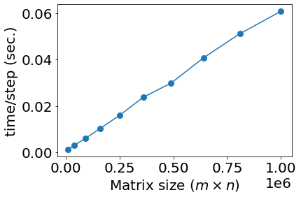
Figure 1: PIOT running time per MC step v.s. matrix size.

[R2, R3] Running time of PIOT method. The experiments are performed on computing clusters with nodes equipped with 40 Intel Xeon 2.10 GHz CPUs and 192 GB memory. The PIOT inference has a linear computational complexity of $\mathcal{O}(mn)$ ($m$ and $n$ are the dimensions of the matrix.) as shown in Fig. 1. The slope can be further reduced by optimizing the implementation, which we have not done. Prediction uses the entropy-regularized OT (EOT). Note that our algorithm is highly parallelizable. Add this plot to camera ready?

[R2] ‘Further quantification and empirical investigation.’ Yes, will do! In practice, cost matrices are not accessible.To verify our method, for synthetic data, we compared our posterior against the ground truth in Fig.4. For real data, as R2 point out, the consistency is verified by ‘transport to cost, and going back from cost to transport’ approach. In revision, we will add further analysis by varying matrix size, choice of hyperparameters and constraint on cost. Do we want to do this?

[R2] Noise(missing) on more than one element. Results hold for the general setting! To simplify the notation, without loss, we assumed noise only occurs on one element (as the general case may be treated as compositions of such). For instance, Prop 3.17 still holds with the modification that the $\mathbb{B}_{a}(T)$ shall contain all the noisy matrices, the distance shall be calculated for two sets of parallel hyperplanes. will add explanation in the main text.

[R4] Experimental settings and conclusions. The parameters for each experiment are provided in the text. For the hardware setting please see the response of Running time of PIOT method. above. For the conclusion, we demonstrate the results in figures and a table with discussions in the text. See, for example, the paragraph starting from line 425, where we discuss the results depicted in Fig. 5. will double check we have these

[R5] Why entropy regularized OT. EOT was chosen because: 1. OT plan is general sparse (deterministic), and zero elements do not carry sufficient information to apply any meaningful inference on the cost. In particular, zero in the plan does not necessarily imply that the corresponding cost is infinity. 2. EOT both takes into account of the uncertainty and incompleteness of observed data, and is faster (Cuturi, 2013). 3. When $\lambda$ goes to 0, it recovers OT. will incorporate to the main text

[R5] Interpretation of the inferred cost. Yes, there is an interpretation. For the European migration data the cost function is not simply the Euclidean distance between countries but could be a combination of complex factors such as ticket prices, international relationships, and languages. To model all the factors is complicated and impractical. Strong priors or constraints may simplify the problem (stuart2020inverse), but uniform priors and softer constraints provide us less-biased results. We develop a probabilistic method, analyze the underlying geometry, and infer the migration costs quantitatively. The inferred cost is then a consequence of the costs from the hidden factors. In Table 1 and the last two paragraphs we consider cases where there is a noise or a missing value, which are common in real world data. We demonstrate that our method accurately predict missing values. will incorporate.

[MR] ‘the authors should make it much more clear that this work address only the *discrete* setting. The word ”discrete” appears only once in the entire draft. Rather, as R2 and R5 recommend, it should appear in the title so as to not give the false impression that the continuous cost setting has been addressed and solved.’ — shall we do this?

[R2] – make all the figures and fonts bigger.

[R5] – Add line numbers to Algorithm 1 may be useful

[R5] – Figure 3: There is no label for the x-axis