Neurashed: A Phenomenological Model for Imitating
Deep Learning Training

Abstract

To advance deep learning methodologies in the next decade, a theoretical framework for reasoning about modern neural networks is needed. While efforts are increasing toward demystifying why deep learning is so effective, a comprehensive picture remains lacking, suggesting that a better theory is possible. We argue that a future deep learning theory should inherit three characteristics: a hierarchically structured network architecture, parameters iteratively optimized using stochastic gradient-based methods, and information from the data that evolves compressively. As an instantiation, we integrate these characteristics into a graphical model called neurashed. This model effectively explains some common empirical patterns in deep learning. In particular, neurashed enables insights into implicit regularization, information bottleneck, and local elasticity. Finally, we discuss how neurashed can guide the development of deep learning theories.

1 Introduction

Deep learning is recognized as a monumentally successful approach to many data-extensive applications in image recognition, natural language processing, and board game programs [1, 2, 3]. Despite extensive efforts [4, 5, 6], however, our theoretical understanding of how this increasingly popular machinery works and why it is so effective remains incomplete. This is exemplified by the substantial vacuum between the highly sophisticated training paradigm of modern neural networks and the capabilities of existing theories. For instance, the optimal architectures for certain specific tasks in computer vision remain unclear [7].

To better fulfill the potential of deep learning methodologies in increasingly diverse domains, heuristics and computation are unlikely to be adequate—a comprehensive theoretical foundation for deep learning is needed. Ideally, this theory would demystify these black-box models, visualize the essential elements, and enable principled model design and training. A useful theory would, at a minimum, reduce unnecessary computational burden and human costs in present-day deep-learning research, even if it could not make all complex training details transparent.

Unfortunately, it is unclear how to develop a deep learning theory from first principles. Instead, in this paper we take a phenomenological approach that captures some important characteristics of deep learning. Roughly speaking, a phenomenological model provides an overall picture rather than focusing on details, and allows for useful intuition and guidelines so that a more complete theoretical foundation can be developed.

To address what characteristics of deep learning should be considered in a phenomenological model, we recall the three key components in deep learning: architecture, algorithm, and data [8]. The most pronounced characteristic of modern network architectures is their hierarchical composition of simple functions. Indeed, overwhelming evidence shows that multiple-layer architectures are superior to their shallow counterparts [9], reflecting the fact that high-level features are hierarchically represented through low-level features [10, 11]. The optimization workhorse for training neural networks is stochastic gradient descent or Adam [12], which iteratively updates the network weights using noisy gradients evaluated from small batches of training samples. Overwhelming evidence shows that the solution trajectories of iterative optimization are crucial to generalization performance [13]. It is also known that the effectiveness of deep learning relies heavily on the structure of the data [14, 15], which enables the compression of data information in the late stages of deep learning training [16, 17].

2 Neurashed

We introduce a simple, interpretable, white-box model that simultaneously possesses the hierarchical, iterative, and compressive characteristics to guide the development of a future deep learning theory. This model, called neurashed, is represented as a graph with nodes partitioned into different levels (Figure 1). The number of levels is the same as the number of layers of the neural network that neurashed imitates. Instead of corresponding with a single neuron in the neural network, an $l$-level node in neurashed represents a feature that the neural network can learn in its $l$-layer. For example, the nodes in the first/bottom level denote lowest-level features, whereas the nodes in the last/top level correspond to the class membership in the classification problem. To describe the dependence of high-level features on low-level features, neurashed includes edges between a node and its dependent nodes in the preceding level. This reflects the hierarchical nature of features in neural networks.

Figure 1: A neurashed model that imitates a four-layer neural network for a three-class classification problem. For instance, the feature represented by the leftmost node in the second level is formed by the features represented by the three leftmost nodes in the first level.

Given any input sample, a node in neurashed is in one of two states: firing or not firing. The unique last-level node that fires for an input corresponds with the label of the input. Whether a node in the first level fires or not is determined by the input. For a middle-level node, its state is determined by the firing pattern of its dependent nodes in the preceding levels. For example, let a node represent cat and its dependent nodes be cat head and cat tail. We activate cat when either or both of the two dependent nodes are firing. Alternatively, let a node represent panda head and consider its dependent nodes dark circle, black ear, and white face. The panda head node fires only if all three dependent nodes are firing.

We call the subgraph induced by the firing nodes the feature pathway of a given input. Samples from different classes have relatively distinctive feature pathways, commonly shared at lower levels but more distinct at higher levels. By contrast, feature pathways of same-class samples are identical or similar. An illustration is given in Figure 2.

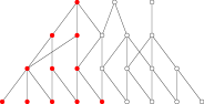
(a) Class 1a

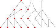
(b) Class 1b

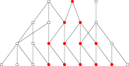
(c) Class 2

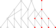
(d) Class 3

Figure 2: Feature pathways of the neurashed model in Figure 1. Firing nodes are marked in red. Class 1 includes two types of samples with slightly different feature pathways, which is a reflection of heterogeneity in real-life data [18].

To enable prediction, all nodes $F$ except for the last-level nodes are assigned a nonnegative value $\lambda_{F}$ as a measure of each node’s ability to sense the corresponding feature. A large value of $\lambda_{F}$ means that when this node fires it can send out strong signals to connected nodes in the next level. Hence, $\lambda_{F}$ is the amplification factor of $F$. Moreover, let $\eta_{fF}$ denote the weight of a connected second-last-level node $f$ and last-level node $F$. Given an input, we define the score of each node, which is sent to its connected nodes on the next level: For any first-level node $F$, let score $S_{F}=\lambda_{F}$ if $F$ is firing and $S_{F}=0$ otherwise; for any firing middle-level node F, we recursively define

$$S_{F}=\lambda_{F}\sum_{f\rightarrow F}S_{f},$$

where the sum is over all dependent nodes $f$ of $F$ in the lower level. Likewise, let $S_{F}=0$ for any non-firing middle-level node $F$. For the last-level nodes $F_{1},\ldots,F_{K}$ corresponding to the $K$ classes, let

$$Z_{j}=\sum_{f\rightarrow{F_{j}}}\eta_{fF_{j}}S_{f}$$ (2.1)

be the logit for the $j$th class, where the sum is over all second-last-level dependent nodes $f$ of $F_{j}$. Finally, we predict the probability that this input is in the $j$th class as

$$p_{j}(x)=\frac{\exp(Z_{j})}{\sum_{i=1}^{K}\exp(Z_{i})}.$$

To mimic the iterative characteristic of neural network training, we must be able to update the amplification factors for neurashed during training. At initialization, because there is no predictive ability as such for neurashed, we set $\lambda_{F}$ and $\eta_{fF}$ to zero, other constants, or random numbers. In each backpropagation, a node is firing if it is in the union of the feature pathways of all training samples in the mini-batch for computing the gradient. We increase the amplification ability of any firing node. Specifically, if a node $F$ is firing in the backpropagation, we update its amplification factor $\lambda_{F}$ by letting

$$\lambda_{F}\leftarrow g^{+}(\lambda_{F}),$$

where $g^{+}$ is an increasing function satisfying $g^{+}(x)>x$ for all $x\geq 0$. The simplest choices include $g^{+}(x)=ax$ for $a>1$ and $g^{+}(x)=x+c$ for $c>0$. The strengthening of firing feature pathways is consistent with a recent analysis of simple hierarchical models [19, 20]. By contrast, for any node $F$ that is not firing in the backpropagation, we decrease its amplification factor by setting

$$\lambda_{F}\leftarrow g^{-}(\lambda_{F})$$

for an increasing function $g^{-}$ satisfying $0\leq g^{-}(x)\leq x$; for example, $g^{-}(x)=bx$ for some $0<b\leq 1$. This recognizes regularization techniques such as weight decay, batch normalization [21], layer normalization [22], and dropout [23] in deep-learning training, which effectively impose certain constraints on the weight parameters [24]. Update rules $g^{+},g^{-}$ generally vary with respect to nodes and iteration number. Likewise, we apply rule $g^{+}$ to $\eta_{fF}$ when the connected second-last-level node $f$ and last-level node $F$ both fire; otherwise, $g^{-}$ is applied.

The training dynamics above could improve neurashed’s predictive ability. In particular, the update rules allow nodes appearing frequently in feature pathways to quickly grow their amplification factors. Consequently, for an input $x$ belonging to the $j$th class, the amplification factors of most nodes in its feature become relatively large during training, and the true-class logit $Z_{j}$ also becomes much larger than the other logits $Z_{i}$ for $i\neq j$. This shows that the probability of predicting the correct class $p_{j}(x)\rightarrow 1$ as the number of iterations tends to infinity.

The modeling strategy of neurashed is similar to a watershed, where tributaries meet to form a larger stream (hence “neurashed”). This modeling strategy gives neurashed the innate characteristics of a hierarchical structure and iterative optimization. As a caveat, we do not regard the feature representation of neurashed as fixed. Although the graph is fixed, the evolving amplification factors represent features in a dynamic manner. Note that neurashed is different from capsule networks [25] and GLOM [10] in that our model is meant to shed light on the black box of deep learning, not serve as a working system.

3 Insights into Puzzles

Implicit regularization. Conventional wisdom from statistical learning theory suggests that a model may not perform well on test data if its parameters outnumber the training samples; to avoid overfitting, explicit regularization is needed to constrain the search space of the unknown parameters [26]. In contrast to other machine learning approaches, modern neural networks—where the number of learnable parameters is often orders of magnitude larger than that of the training samples—enjoy surprisingly good generalization even without explicit regularization [27]. From an optimization viewpoint, this shows that simple stochastic gradient-based optimization for training neural networks implicitly induces a form of regularization biased toward local minima of low “complexity” [13, 28]. However, it remains unclear how implicit regularization occurs from a geometric perspective [29, 30, 31].

To gain geometric insights into implicit regularization using our conceptual model, recall that only firing features grow during neurashed training, whereas the remaining features become weaker during backpropagation. For simplicity, consider stochastic gradient descent with a mini-batch size of 1. Here, only common features shared by samples from different classes constantly fire in neurashed, whereas features peculiar to some samples or certain classes fire less frequently. As a consequence, these common features become stronger more quickly, whereas the other features grow less rapidly or even diminish.

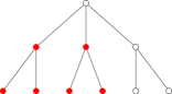
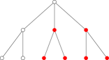
Small-batch training

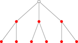
Large-batch training

Figure 3: Part of neurashed that corresponds to a single class. The two top plots in the left panel show two feature pathways, and the top plot in the right panel denotes the firing pattern when both feature pathways are included in the batch (the last-level node is firing but is not marked in red for simplicity). The two bottom plots represent the learned neurashed models, where larger nodes indicate larger amplification factors.

When gradient descent or large-batch stochastic gradient descent are used, many features fire in each update of neurashed, thereby increasing their amplification factors simultaneously. By contrast, a small-batch method constructs the feature pathways in a sparing way. Consequently, the feature pathways learned using small batches are sparser, suggesting a form of compression. This comparison is illustrated in Figure 3, which implies that different samples from the same class tend to exhibit vanishing variability in their high-level features during later training, and is consistent with the recently observed phenomenon of neural collapse [32]. Intuitively, this connection is indicative of neurashed’s compressive nature.

Although neurashed’s geometric characterization of implicit regularization is currently a hypothesis, much supporting evidence has been reported, empirically and theoretically. Empirical studies in [33, 34] showed that neural networks trained by small-batch methods generalize better than when trained by large-batch methods. Moreover, [35, 36] showed that neural networks tend to be more accurate on test data if these models leverage less information of the images. From a theoretical angle, [37] related generalization performance to a solution’s sparsity level when a simple nonlinear model is trained using stochastic gradient descent.

Information bottleneck. In [16, 17], the information bottleneck theory of deep learning was introduced, based on the observation that neural networks undergo an initial fitting phase followed by a compression phase. In the initial phase, neural networks seek to both memorize the input data and fit the labels, as manifested by the increase in mutual information between a hidden level and both the input and labels. In the second phase, the networks compress all irrelevant information from the input, as demonstrated by the decrease in mutual information between the hidden level and input.

Instead of explaining how this mysterious phenomenon emerges in deep learning, which is beyond our scope, we shed some light on information bottleneck by producing the same phenomenon using neurashed. As with implicit regularization, we observe that neurashed usually contains many redundant feature pathways when learning class labels. Initially, many nodes grow and thus encode more information regarding both the input and class labels. Subsequently, more frequently firing nodes become more dominant than less frequently firing ones. Because nodes compete to grow their amplification factors, dominant nodes tend to dwarf their weaker counterparts after a sufficient amount of training. Hence, neurashed starts to “forget” the information encoded by the weaker nodes, thereby sharing less mutual information with the input samples (see an illustration in Figure 4). The compressive characteristic of neurashed arises, loosely speaking, from the internal competition among nodes. This interpretation of the information bottleneck via neurashed is reminiscent of the human brain, which has many neuron synapses during childhood that are pruned to leave fewer firing connections in adulthood [38].

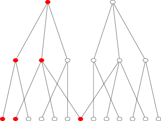
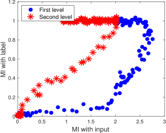
Figure 4: A neurashed model for a binary classification problem. All four firing patterns of Class 1 on the first level (from left to right): $(1,2,7),(2,3,7),(4,5,7),(5,6,7)$. In the second level, the first and third nodes fire if one or more dependent nodes fire, and the second (dominant) node fires if two or more dependent nodes fire. The left panel displays a feature pathway of Class 1. Class 2 has four feature pathways that are symmetric to those of Class 1. The right panel shows the information bottleneck phenomenon for this neurashed model. As with [17], noise is added in calculating the mutual information (MI) between the first/second level and the input (8 types)/labels (2 types). More details are given in the appendix.

Local elasticity. Last, we consider a recently observed phenomenon termed local elasticity [39] in deep learning training, which asks how the update of neural networks via backpropagation at a base input changes the prediction at a test sample. Formally, for $K$-class classification, let $z_{1}(x,w),\ldots,z_{K}(x,w)$ be the logits prior to the softmax operation with input $x$ and network weights $w$. Writing $w^{+}$ for the updated weights using the base input $x$, we define

$$\mathrm{LE}(x,x^{\prime}):=\frac{\sqrt{\sum_{i=1}^{K}(z_{i}(x^{\prime},w^{+})-z_{i}(x^{\prime},w))^{2}}}{\sqrt{\sum_{i=1}^{K}(z_{i}(x,w^{+})-z_{i}(x,w))^{2}}}$$

as a measure of the impact of base $x$ on test $x^{\prime}$. A large value of this measure indicates that the base has a significant impact on the test input. Through extensive experiments, [39] demonstrated that well-trained neural networks are locally elastic in the sense that the value of this measure depends on the semantic similarity between two samples $x$ and $x^{\prime}$. If they are similar—say, images of a cat and tiger—the impact is significant, and if they are dissimilar—say, images of a cat and turtle—the impact is low. Experimental results are shown in Figure 5. For comparison, local elasticity does not appear in linear classifiers because of the leverage effect. More recently, [40, 41, 42] showed that local elasticity implies good generalization ability.

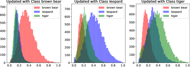
Figure 5: Histograms of $\mathrm{LE}(x,x^{\prime})$ evaluated on the pre-trained VGG-19 network [43]. For example, in the left panel the base input $x$ are images of brown bears. Each class contains 120 images sampled from ImageNet [44]. Tiger and leopard are felines and similar.

We now show that neurashed exhibits the phenomenon of local elasticity, which yields insights into how local elasticity emerges in deep learning. To see this, note that similar training samples share more of their feature pathways. For example, the two types of samples in Class 1 in Figure 2 are presumably very similar and indeed have about the same feature pathways; Class 1 and Class 2 are more similar to each other than Class 1 and Class 3 in terms of feature pathways. Metaphorically speaking, applying backpropagation at an image of a leopard, the feature pathway for leopard strengthens as the associated amplification factors increase. While this update also strengthens the feature pathway for tiger, it does not impact the brown bear feature pathway as much, which presumably overlaps less with the leopard feature pathway. This update in turn leads to a more significant change in the logits (2.1) of an image of a tiger than those of a brown bear. Returning to Figure 2 for an illustration of this interpretation, the impact of updating at a sample in Class 1a is most significant on Class 1b, less significant on Class 2, and unnoticeable on Class 3.

4 Outlook

In addition to shedding new light on implicit regularization, information bottleneck, and local elasticity, neurashed is likely to facilitate insights into other common empirical patterns of deep learning. First, a byproduct of our interpretation of implicit regularization might evidence a subnetwork with comparable performance to the original, which could have implications on the lottery ticket hypothesis of neural networks [45]. Second, while a significant fraction of classes in ImageNet [44] have fewer than 500 training samples, deep neural networks perform well on these classes in tests. Neurashed could offer a new perspective on these seemingly conflicting observations—many classes are basically the same (for example, ImageNet contains 120 dog-breed classes), so the effective sample size for learning the common features is much larger than the size of an individual class. Last, neurashed might help reveal the benefit of data augmentation techniques such as cropping. In the language of neurashed, cat head and cat tail each are sufficient to identify cat. If both concepts appear in the image, cropping reinforces the neurashed model by impelling it to learn these concepts separately. Nevertheless, these views are preliminary and require future consolidation.

While closely resembling neural networks in many aspects, neurashed is not merely intended to better explain some phenomena in deep learning. Instead, our main goal is to offer insights into the development of a comprehensive theoretical foundation for deep learning in future research. In particular, neurashed’s efficacy in interpreting many puzzles in deep learning could imply that neural networks and neurashed evolve similarly during training. We therefore believe that a comprehensive deep learning theory is unlikely without incorporating the hierarchical, iterative, and compressive characteristics. That said, useful insights can be derived from analyzing models without these characteristics in some specific settings [4, 46, 47, 48, 49, 50, 51, 52, 53, 54].

Integrating the three characteristics in a principled manner might necessitate a novel mathematical framework for reasoning about the composition of nonlinear functions. Because it could take years before such mathematical tools become available, a practical approach for the present, given that such theoretical guidelines are urgently needed [55], is to better relate neurashed to neural networks and develop finer-grained models. For example, an important question is to determine the unit in neural networks that corresponds with a feature node in neurashed. Is it a filter in the case of convolutional neural networks? Another topic is the relationship between neuron activations in neural networks and feature pathways in neurashed. To generalize neurashed, edges could be fired instead of nodes. Another potential extension is to introduce stochasticity to rules $g^{+}$ and $g^{-}$ for updating amplification factors and rendering feature pathways random or adaptive to learned amplification factors. Owing to the flexibility of neurashed as a graphical model, such possible extensions are endless.

Acknowledgments

We would like to thank Patrick Chao, Zhun Deng, Cong Fang, Hangfeng He, Qingxuan Jiang, Konrad Kording, Yi Ma, and Jiayao Zhang for helpful discussions and comments. This work was supported in part by NSF through CAREER DMS-1847415 and CCF-1934876, an Alfred Sloan Research Fellowship, and the Wharton Dean’s Research Fund.

Appendix

All eight feature pathways of the neurashed model in Figure 4. The left column and right column correspond to Class 1 and Class 2, respectively.

In the experimental setup of the right panel of Figure 4, all amplification factors at initialization are set to independent uniform random variables on $(0,0.01)$. We use $g^{-}(\lambda_{F})=1.022^{-\frac{1}{4}}\lambda_{F}$ and $g^{+}(\lambda_{F})=1.022^{\frac{11}{4}}\lambda_{F}$ for all hidden nodes except for the 7th (from left to right) node, which uses $g^{+}(\lambda_{F})=1.022^{\frac{3}{4}}\lambda_{F}$. In the early phase of training, the firing pattern on the second level improves at distinguishing the two types of samples in Class 1, depending on whether the 1st or 3rd node fires. This also applies to Class 2. Hence, the mutual information between the second level and the input tends to $\log_{2}4=2$. By contrast, in the late stages, the amplification factors of the 1st and 3rd nodes become negligible compared with that of the 2nd node, leading to indistinguishability between the two types in Class 1. As a consequence, the mutual information tends to $\log_{2}2=1$. The discussion on the first level is similar and thus is omitted.

References

- [1] Alex Krizhevsky, Ilya Sutskever and Geoffrey E Hinton “Imagenet classification with deep convolutional neural networks” In Communications of the ACM 60.6 AcM New York, NY, USA, 2017, pp. 84–90
- [2] Yann LeCun, Yoshua Bengio and Geoffrey Hinton “Deep learning” In Nature 521.7553 Nature Publishing Group, 2015, pp. 436–444
- [3] David Silver et al. “Mastering the game of Go with deep neural networks and tree search” In Nature 529.7587 Nature Publishing Group, 2016, pp. 484–489
- [4] Arthur Jacot, Franck Gabriel and Clément Hongler “Neural tangent kernel: convergence and generalization in neural networks” In Advances in Neural Information Processing Systems, 2018, pp. 8580–8589
- [5] Peter L Bartlett, Dylan J Foster and Matus Telgarsky “Spectrally-normalized margin bounds for neural networks” In Advances in Neural Information Processing Systems, 2017, pp. 6241–6250
- [6] Julius Berner, Philipp Grohs, Gitta Kutyniok and Philipp Petersen “The Modern Mathematics of Deep Learning” In arXiv preprint arXiv:2105.04026, 2021
- [7] Ilya Tolstikhin et al. “MlP-mixer: An all-MLP architecture for vision” In arXiv preprint arXiv:2105.01601, 2021
- [8] Lenka Zdeborová “Understanding deep learning is also a job for physicists” In Nature Physics 16.6 Nature Publishing Group, 2020, pp. 602–604
- [9] Ronen Eldan and Ohad Shamir “The power of depth for feedforward neural networks” In Conference on Learning Theory, 2016, pp. 907–940 PMLR
- [10] Geoffrey Hinton “How to represent part-whole hierarchies in a neural network” In arXiv preprint arXiv:2102.12627, 2021
- [11] Andrey A Bagrov, Ilia A Iakovlev, Askar A Iliasov, Mikhail I Katsnelson and Vladimir V Mazurenko “Multiscale structural complexity of natural patterns” In Proceedings of the National Academy of Sciences 117.48 National Acad Sciences, 2020, pp. 30241–30251
- [12] Diederik P Kingma and Jimmy Ba “Adam: A Method for Stochastic Optimization” In International Conference on Learning Representations, 2015
- [13] Daniel Soudry, Elad Hoffer, Mor Shpigel Nacson, Suriya Gunasekar and Nathan Srebro “The implicit bias of gradient descent on separable data” In The Journal of Machine Learning Research 19.1 JMLR. org, 2018, pp. 2822–2878
- [14] Avrim L Blum and Ronald L Rivest “Training a 3-node neural network is NP-complete” In Neural Networks 5.1 Elsevier, 1992, pp. 117–127
- [15] Sebastian Goldt, Marc Mézard, Florent Krzakala and Lenka Zdeborová “Modeling the Influence of Data Structure on Learning in Neural Networks: The Hidden Manifold Model” In Physical Review X 10.4 APS, 2020, pp. 041044
- [16] Naftali Tishby and Noga Zaslavsky “Deep learning and the information bottleneck principle” In 2015 IEEE Information Theory Workshop (ITW), 2015, pp. 1–5 IEEE
- [17] Ravid Shwartz-Ziv and Naftali Tishby “Opening the black box of deep neural networks via information” In arXiv preprint arXiv:1703.00810, 2017
- [18] Vitaly Feldman “Does learning require memorization? a short tale about a long tail” In Symposium on Theory of Computing, 2020, pp. 954–959
- [19] Tomaso Poggio, Andrzej Banburski and Qianli Liao “Theoretical issues in deep networks” In Proceedings of the National Academy of Sciences 117.48 National Acad Sciences, 2020, pp. 30039–30045
- [20] Zeyuan Allen-Zhu and Yuanzhi Li “Backward feature correction: How deep learning performs deep learning” In arXiv preprint arXiv:2001.04413, 2020
- [21] Sergey Ioffe and Christian Szegedy “Batch normalization: Accelerating deep network training by reducing internal covariate shift” In International Conference on Machine Learning, 2015, pp. 448–456 PMLR
- [22] Jimmy Lei Ba, Jamie Ryan Kiros and Geoffrey E Hinton “Layer normalization” In arXiv preprint arXiv:1607.06450, 2016
- [23] Nitish Srivastava, Geoffrey Hinton, Alex Krizhevsky, Ilya Sutskever and Ruslan Salakhutdinov “Dropout: A simple way to prevent neural networks from overfitting” In The Journal of Machine Learning Research 15.1 JMLR. org, 2014, pp. 1929–1958
- [24] Cong Fang, Hangfeng He, Qi Long and Weijie J Su “Exploring Deep Neural Networks via Layer-Peeled Model: Minority Collapse in Imbalanced Training” In Proceedings of the National Academy of Sciences, 2021
- [25] Sara Sabour, Nicholas Frosst and Geoffrey E Hinton “Dynamic routing between capsules” In Advances in Neural Information Processing Systems 31, 2017, pp. 3859–3869
- [26] Jerome Friedman, Trevor Hastie and Robert Tibshirani “The elements of statistical learning” Springer Series in Statistics New York, 2001
- [27] Chiyuan Zhang, Samy Bengio, Moritz Hardt, Benjamin Recht and Oriol Vinyals “Understanding deep learning (still) requires rethinking generalization” In Communications of the ACM 64.3 ACM New York, NY, USA, 2021, pp. 107–115
- [28] Peter L Bartlett, Philip M Long, Gábor Lugosi and Alexander Tsigler “Benign overfitting in linear regression” In Proceedings of the National Academy of Sciences 117.48 National Acad Sciences, 2020, pp. 30063–30070
- [29] Vaishnavh Nagarajan and J. Zico Kolter “Uniform convergence may be unable to explain generalization in deep learning” In Advances in Neural Information Processing Systems 32, 2019
- [30] Noam Razin and Nadav Cohen “Implicit Regularization in Deep Learning May Not Be Explainable by Norms” In Advances in Neural Information Processing Systems 33, 2020
- [31] Zhi-Hua Zhou “Why over-parameterization of deep neural networks does not overfit?” In Science China Information Sciences 64.1 Science China Press, 2021, pp. 1–3
- [32] Vardan Papyan, XY Han and David L Donoho “Prevalence of neural collapse during the terminal phase of deep learning training” In Proceedings of the National Academy of Sciences 117.40 National Acad Sciences, 2020, pp. 24652–24663
- [33] Nitish Shirish Keskar, Dheevatsa Mudigere, Jorge Nocedal, Mikhail Smelyanskiy and Ping Tak Peter Tang “On large-batch training for deep learning: Generalization gap and sharp minima” In arXiv preprint arXiv:1609.04836, 2016
- [34] Samuel Smith, Erich Elsen and Soham De “On the Generalization Benefit of Noise in Stochastic Gradient Descent” In International Conference on Machine Learning, 2020, pp. 9058–9067 PMLR
- [35] Andrew Ilyas, Shibani Santurkar, Logan Engstrom, Brandon Tran and Aleksander Madry “Adversarial Examples Are Not Bugs, They Are Features” In Advances in Neural Information Processing Systems 32, 2019
- [36] Kai Xiao, Logan Engstrom, Andrew Ilyas and Aleksander Madry “Noise or signal: The role of image backgrounds in object recognition” In International Conference on Learning Representations, 2021
- [37] Jeff Z HaoChen, Colin Wei, Jason D Lee and Tengyu Ma “Shape matters: Understanding the implicit bias of the noise covariance” In arXiv preprint arXiv:2006.08680, 2020
- [38] Irwin Feinberg “Schizophrenia: caused by a fault in programmed synaptic elimination during adolescence?” In Journal of Psychiatric Research 17.4 Elsevier, 1982, pp. 319–334
- [39] Hangfeng He and Weijie J Su “The Local Elasticity of Neural Networks” In International Conference on Learning Representations, 2020
- [40] Shuxiao Chen, Hangfeng He and Weijie J Su “Label-Aware Neural Tangent Kernel: Toward Better Generalization and Local Elasticity” In Advances in Neural Information Processing Systems 33, 2020, pp. 15847–15858
- [41] Zhun Deng, Hangfeng He and Weijie J Su “Toward Better Generalization Bounds with Locally Elastic Stability” In International Conference on Machine Learning, 2021
- [42] Jiayao Zhang, Hua Wang and Weijie J Su “Imitating Deep Learning Dynamics via Locally Elastic Stochastic Differential Equations” In Advances in Neural Information Processing Systems 34, 2021
- [43] Karen Simonyan and Andrew Zisserman “Very deep convolutional networks for large-scale image recognition” In arXiv preprint arXiv:1409.1556, 2014
- [44] Jia Deng, Wei Dong, Richard Socher, Li-Jia Li, Kai Li and Li Fei-Fei “ImageNet: A large-scale hierarchical image database” In 2009 IEEE Conference on Computer Vision and Pattern Recognition, 2009, pp. 248–255 IEEE Computer Society
- [45] Jonathan Frankle and Michael Carbin “The Lottery Ticket Hypothesis: Finding Sparse, Trainable Neural Networks” In International Conference on Learning Representations, 2018
- [46] Lenaic Chizat, Edouard Oyallon and Francis Bach “On lazy training in differentiable programming” In Advances in Neural Information Processing Systems, 2019
- [47] Lei Wu, Chao Ma and Weinan E “How SGD selects the global minima in over-parameterized learning: A dynamical stability perspective” In Advances in Neural Information Processing Systems, 2018, pp. 8289–8298
- [48] Song Mei, Andrea Montanari and Phan-Minh Nguyen “A mean field view of the landscape of two-layer neural networks” In Proceedings of the National Academy of Sciences 115.33 National Academy of Sciences, 2018, pp. E7665–E7671
- [49] Lénaïc Chizat and Francis Bach “On the global convergence of gradient descent for over-parameterized models using optimal transport” In Advances in Neural Information Processing Systems, 2018, pp. 3040–3050
- [50] Mikhail Belkin, Daniel Hsu, Siyuan Ma and Soumik Mandal “Reconciling modern machine-learning practice and the classical bias–variance trade-off” In Proceedings of the National Academy of Sciences 116.32 National Acad Sciences, 2019, pp. 15849–15854
- [51] Jaehoon Lee, Lechao Xiao, Samuel S Schoenholz, Yasaman Bahri, Roman Novak, Jascha Sohl-Dickstein and Jeffrey Pennington “Wide neural networks of any depth evolve as linear models under gradient descent” In arXiv preprint arXiv:1902.06720, 2019
- [52] Zhi-Qin John Xu, Yaoyu Zhang and Yanyang Xiao “Training behavior of deep neural network in frequency domain” In International Conference on Neural Information Processing, 2019, pp. 264–274 Springer
- [53] Samet Oymak and Mahdi Soltanolkotabi “Towards moderate overparameterization: global convergence guarantees for training shallow neural networks” In IEEE Journal on Selected Areas in Information Theory IEEE, 2020
- [54] Kwan Ho Ryan Chan, Yaodong Yu, Chong You, Haozhi Qi, John Wright and Yi Ma “ReduNet: A White-box Deep Network from the Principle of Maximizing Rate Reduction” In arXiv preprint arXiv:2105.10446, 2021
- [55] Weinan E “The dawning of a new era in applied mathematics” In Notices of the American Mathematical Society 68.4 American Mathematical Society, 2021, pp. 565–571