Solar mass black holes from neutron stars and bosonic dark matter

Abstract

Black holes with masses $\approx 1\,M_{\odot}$ cannot be produced via stellar evolution. A popular scenario of their formation involves transmutation of neutron stars — by accumulation of dark matter triggering gravitational collapse in the star centers. We show that this scenario can be realized in the models of bosonic dark matter despite the apparently contradicting requirements on the interactions of dark matter particles: on the one hand, they should couple to neutrons strongly enough to be captured inside the neutron stars, on the other, their loop–induced self–interactions impede collapse. Observing that these conflicting conditions are imposed at different scales, we demonstrate that models with efficient accumulation of dark matter can be deformed at large fields to make unavoidable its subsequent collapse into a black hole. Workable examples include weakly coupled models with bended infinite valleys.

I Introduction

The existing gravitational wave detectors are sensitive to compact objects — black holes (BHs) and neutron stars (NSs) — of masses ranging from tens of solar masses down to $M_{\odot}$, see Abbott et al. (2017, 2021a). Thus far, few tens of coalescing BHs and several BH–NS systems were detected Abbott et al. (2019, 2021b, 2021c, 2021d), while hundreds of observations are further expected in the near future. This will be sufficient to map out the mass function of the stellar–size BHs.

Standard stellar evolution predicts no BHs lighter than the heaviest neutron stars, as the Fermi pressure stabilizes the neutron cores at masses below ${2.5M_{\odot}}$, cf. Rhoades and Ruffini (1974); Lattimer (2012); Özel and Freire (2016). The BH mass function is hence expected to have a gap below this value, and any detection in that region would automatically imply existence of an exotic mechanism for black hole formation. We will refer to such light BHs as “solar mass black holes.”

A widely discussed possibility is production of solar mass BHs in the early Universe from small–scale density perturbations. It has a natural extension: these objects may also play the role of dark matter (DM). The latter hypothesis, however, is strongly constrained by lensing Tisserand et al. (2007), CMB measurements Ricotti et al. (2008); Ali-Haïmoud and Kamionkowski (2017), and even the gravitational wave observations themselves Sasaki et al. (2018).

Alternatively, the solar mass BHs may appear in the present Universe due to neutron star collapses caused by seed BHs Goldman and Nussinov (1989). The latter BHs may in turn be of primordial origin, and be small enough to evade the lensing and CMB constraints. This option, however, still relies on cosmology to produce a sufficient seed BH population.

A more intriguing possibility is the formation of seed BHs through the gravitational collapse of dark matter accumulated by old neutron stars Kouvaris and Tinyakov (2011a, b); McDermott et al. (2012); Bell et al. (2013); Kouvaris et al. (2018); Garani et al. (2019); Dasgupta et al. (2021). A sufficient accumulation is possible only if the DM is asymmetric Davoudiasl and Mohapatra (2012) and does not annihilate in the stellar core. In the simplest case one assumes that the DM particles carry a conserved global charge ensuring their stability, and their antiparticles disappear during the early stages of cosmological evolution.

In the present paper we focus on the last scenario. Our goal is to identify DM models where such catalyzed transmutation of the neutron stars into the solar mass BHs can take place. The mechanism we consider involves four stages: (i) capture of DM by the neutron star; (ii) its thermalization; (iii) concentration in the star center and gravitational collapse into a seed BH; (iv) accretion of the star material onto the BH and formation of the solar mass BH. Given the DM abundance, the stage (i) sets the maximum mass of DM that can be accumulated by the neutron star. On the other hand, the stage (iii) requires some minimum amount of DM for the successful gravitational collapse. The viability of the overall scenario depends on the possibility to satisfy both requirements in the same DM model.

Stages (i), (ii), and (iv), i.e. the beginning of the process and its very end, have been extensively discussed in the literature, see the review Tinyakov et al. and Kouvaris and Tinyakov (2014); Génolini et al. (2020). We will provide a short summary of these results in the next section. The main part of this paper considers model–dependent evolution and gravitational collapse of dense dark matter cloud at stage (iii).

The minimum number of particles required for collapse is different in the cases of bosonic and fermionic dark matter, and crucially depends on the DM self–interactions. In the ensemble of free DM fermions, the Fermi pressure balances self–gravity and halts the gravitational collapse unless the total particle number exceeds the (analog of the) Chandrasekhar limit Chandrasekhar (1931),

$$\text{free fermions:}\quad N_{cr}\sim\left({M_{\rm Pl}\over m}\right)^{3}\sim 10^{57}\left({{\rm GeV}\over m}\right)^{3}\,,$$ (1)

where $m$ is the DM mass. This number is prohibitively large unless $m$ is in the 100 TeV range or above Kouvaris et al. (2018). While not necessarily impossible, such scenarios with super-heavy asymmetric dark matter are outside of the mainstream cosmological models, and we do not consider them here.

If the DM is bosonic and non–interacting, the gravitational attraction of its particles is balanced by the kinetic (“quantum”) pressure guaranteed by the uncertainty principle. Gravitational collapse happens if the particle number exceeds the critical value

$$\text{free bosons:}\quad N_{cr}\sim\left({M_{\rm Pl}\over m}\right)^{2}\sim 10^{38}\left({{\rm GeV}\over m}\right)^{2}\,,$$ (2)

which is parametrically smaller than in the case of fermions. Bosonic DM is therefore a more promising candidate for the creation of seed BHs. In the rest of this paper we will focus on bosons.

While looking advantageous in the free case, Eq. (2), however, can be ruined by very weak DM self–interactions which are generically present in our scenario. Indeed, DM capture and thermalization at stages (i) and (ii) are possible only for sufficiently strong DM–nucleon interactions which in turn induce DM self–couplings via loops Bell et al. (2013). In the simple one–field models, the induced terms in the DM potential are quartic in fields and should be positive, i.e. repulsive, for vacuum stability. In effect, they generically oppose the gravitational collapse and increase the required critical DM multiplicity to unacceptably large values. We have therefore conflicting conditions on the DM model.

In this paper we show that the conflict can be resolved. Namely, the number of DM particles required for collapse can be almost as small as in Eq. (2), and all of these particles can be accumulated inside the neutron star by scattering off nucleons. We start by clarifying and quantifying the requirements on the DM models. Then we propose a generic mechanism to satisfy them simultaneously. We find that the smallest DM multiplicity for collapse is achieved in the models where: (i) the DM potential includes a long valley extending to large, in some cases Planckian fields, and the cutoff of this potential is high enough; (ii) both attractive and repulsive self–interactions are suppressed along this valley; (iii) loop quantum corrections from interactions with the visible sector do not break the condition (ii).

Our mechanism is based on the fact that the conflicting requirements are imposed at different scales. The DM capture depends on the physics in the vicinity of vacuum, while self–interactions obstructing the gravitational collapse should vanish at strong fields. Thus, one can make the potential valley bended in the field space. It may start going along the dark matter field $\phi$, then take a turn at some $|\phi|\gtrsim\Lambda$ and continue in the direction of another field $\chi$. In this case the interaction of $\phi$–particles with nucleons, as we will argue, does not generate an effective potential for $\chi$, and the latter may grow and collapse into a BH almost as in the free bosonic case.

The rest of this paper is organized as follows. We review accumulation and thermalization of DM inside the neutron stars in Sec. II. General requirements on the DM models with the smallest critical multiplicities for gravitational collapse are derived in Sec. III. In Sec IV we propose a mechanism to satisfy these requirements. We conclude in Sec. V.

II DM inside the neutron star

In this section we summarize the existing results on DM capture and thermalization in the neutron star. Two points will be essential for us: (i) the total amount of captured DM and its dependence on the strength of DM–neutron interactions; (ii) the fact that with time this DM forms a Bose–Einstein condensate described by classical fields.

For concreteness we will assume that the DM particles are globally charged scalars with mass $m$ belonging to the typical WIMP range from GeV to a few TeV.

II.1 DM capture

Two generic mechanisms trap DM inside the neutron star: accumulation during the star lifetime and gravitational capture at the star formation. These mechanisms are cumulative. Potentially, they may provide comparable amounts of trapped DM.

In the next sections we consider accumulation of DM particles from the ambient galactic halo Press and Spergel (1985); Gould (1988). Far away from the neutron star, the distribution of DM velocities is nearly Maxwellian with small dispersion ${\bar{v}}^{2}$, e.g. $\bar{v}\sim 10^{-3}$ in the Milky Way. But the particles acquire semi–relativistic speeds ${\sim 0.5}$ as they fall into the neutron star. With masses in the WIMP range, they lose energies of order $m_{n}$ — the neutron’s rest mass — in collisions with neutrons. This is much larger than the asymptotic energies of the particles; thus, most of them bind gravitationally to the neutron star after the first collision. Besides, the momentum transfer in their collisions marginally exceeds the Fermi momentum of neutrons, so that the degeneracy of the latter does not play a crucial role. Neglecting the degeneracy is a crude approximation that overestimates the capture rate Bell et al. (2020, 2021a); Anzuini et al. , but in view of comparable astrophysical uncertainties we will use it for simplicity. Finally, we will ignore general relativity effects which enhance the capture rate by an order 1 number, see Ref. Kouvaris (2008).

Under these assumptions, the capture rate, i.e. the number of trapped DM particles per unit time, takes the form Press and Spergel (1985); Gould (1988),

$$\frac{dN}{dt}\approx\sqrt{24\pi}\,G\;{\rho_{\rm DM}\over m\bar{v}}\,M_{*}R_{*}f\,.$$ (3)

Here $\rho_{\rm DM}$ is ambient DM density, $M_{*}$ and $R_{*}$ represent the mass and the radius of the neutron star, and we introduced the probability $f\leq 1$ for the DM particle to scatter during one pass through the star. The value of $f$ is proportional to the DM–neutron cross section $\sigma$,

$$f={\sigma/\sigma_{\rm crit}}\qquad\mbox{if}\qquad\sigma<\sigma_{\rm crit}\,,$$ (4)

and $f=1$ otherwise. Here the proportionality coefficient (“critical” cross section Press and Spergel (1985)) depends on the neutron star parameters,

$$\sigma_{\rm crit}\sim R_{*}^{2}m_{n}/M_{*}\sim 10^{-45}{\rm cm}^{2}\;,$$

where we used ${M_{*}\sim 1.5\,M_{\odot}}$ and ${R_{*}\sim 10\;\mbox{km}}$ in the estimate. Notably, $\sigma_{\mathrm{crit}}$ is comparable to the upper limits on the DM–nucleon cross section coming from the direct detection experiments Akerib et al. (2017); Aprile et al. (2018); Xia et al. (2019); Aprile et al. (2019); Amole et al. (2019).

Since $dN/dt\propto m^{-1}$, the accumulation rate of dark mass does not directly depend on $m$. Integrating Eq. (3), we obtain the total DM mass inside the 10 Gyr old neutron star,

$$\text{MW}:~{}M_{\rm tot} \sim 7\times 10^{42}\,{\rm GeV}f\sim 7\times 10^{-15}M_{\odot}f,$$ (5)

$$\text{dwarf}:~{}M_{\rm tot} \sim 8\times 10^{46}\,{\rm GeV}f\sim 7\times 10^{-11}M_{\odot}f\,.$$ (6)

The above two options differ by the parameters of the ambient DM distribution: $\bar{v}\approx 220$ km/s, ${\rho_{\rm DM}\approx 0.3}$ GeV/cm³ in the Milky Way (MW) and ${\bar{v}\sim 7}$ km/s, ${\rho_{\rm DM}\sim 100}$ GeV/cm³ in the densest dwarf galaxies Strigari et al. (2007, 2008). Besides, taking $f=1$ turns the above estimates into model–independent upper limits on the total DM mass that can be captured by the neutron star in the respective environments.

Another possibility is a gravitational trapping of the DM during formation of the neutron star Capela et al. (2013, 2014). The latter objects are created in the supernova collapses of ordinary stars with masses above $\sim 9M_{\odot}$, which, in turn, are born in giant molecular clouds. Originally, as the baryonic gas contracts adiabatically into a proca star, a low–velocity fraction of the ambient DM gets trapped by its gravitational well. Eventually, this DM ends up in the center of a heavy progenitor star; estimates of Capela et al. (2013, 2014) show that the captured DM mass is close to Eqs. (5), (6) within an order of magnitude. Later, a fraction of the star DM is inherited by the neutron star in the course of supernova collapse. That last process has never been considered in the literature, but our rough estimate suggests that the respective suppression of $M_{\rm tot}$ lies between $1$ and $10^{-3}$.

In the rest of this paper we will use Eqs. (5), (6) and ignore the second, “gravitational capture” mechanism despite the fact that it seems less sensitive to non–gravitational DM interactions. Indeed, that additional mechanism cannot dramatically change the amount of captured DM even in the best case. Besides, it depends on the multi–stage neutron star formation which is subject to large astrophysical uncertainties. Finally, it does in fact rely on the DM–DM and DM–neutron interactions, albeit in a subtle and indirect way: the non–gravitational couplings are needed to thermalize the DM particles inside the progenitor star and mix them in the phase space, or none would lose enough energy to get into the neutron star.

II.2 Thermalization and condensation

Once gravitationally bound, the DM particles settle on star–crossing orbits and continue to lose energies in repeating collisions with neutrons until a thermal equilibrium is reached. Their kinetic energies reduce to the neutron star temperature ${T\sim 10^{5}}$ K and their orbits shrink to the “thermal” radius,

$$r_{\rm th}\approx\left({9T\over 8\pi G\rho_{c}m}\right)^{1/2}\sim 20\,{\rm cm}\left({100\,{\rm GeV}\over m}\right)^{1/2}\,,$$ (7)

where we substituted the density ${\rho_{c}\sim 10^{15}}$ g/cm³ of the neutron star core. The particles steadily arrive into the central DM cloud during the entire lifetime of the neutron star with the rate (3).

The characteristic time of this thermalization process was estimated in Refs. Goldman and Nussinov (1989); Garani et al. (2021). For almost any model within our scenario, it is much shorter than the age of the Universe  Goldman and Nussinov (1989). Indeed, we had already mentioned that BH formation requires a large number of DM particles inside the neutron star Bell et al. (2013). To capture all of them, one usually assumes the largest possible DM–neutron cross section ${\sigma\sim\sigma_{\mathrm{crit}}}$, and even that may be insufficient. With these interactions, the DM particles equilibrate quickly, since every star crossing in the beginning of the process leads to scattering. On the other hand, we will be able to consider very small DM–neutron cross sections once the new mechanism for reducing the required multiplicity to Eq. (2) is invoked. In that case a necessity to thermalize the DM imposes the strongest constraint on its interactions with neutrons.

As the DM particles continue to accumulate, the multiplicity $N$ of the central cloud grows at a fixed radius (7). Eventually, the mean distance between the particles $r_{\mathrm{th}}N^{-1/3}$ drops below the size $(mT)^{-1/2}$ of their wave functions. This happens at

$$\mathrm{BEC:}\;\;\;\;N\gtrsim 0.2\;T^{3}M_{pl}^{3}\,\rho_{c}^{-3/2}\sim 10^{36}\,,$$ (8)

i.e. significantly before the maximal number of particles (5), (6) is reached. At this point the particle wave functions start to overlap and Bose–Einstein condensate forms in the thermal cloud Semikoz and Tkachev (1995); Khlebnikov and Tkachev (2000); Levkov et al. (2018); Chen et al. (2021). Since then, most of the thermalized DM particles occupy the lowest level in the combined DM and neutron star gravitational potential, with the thermal energy being carried by a few remaining particles.

Thanks to large occupation numbers (8), the Bose–Einstein condensate at the lowest level can be described by a classical DM field $\phi(x)$. From the very beginning it forms a non-rotating Dmitriev et al. (2021) self–bound soliton which is almost detached from the neutron star surroundings. Indeed, even at multiplicity (8) the gravitational field of this object can be estimated to exceed the neutron star’s, and with time the soliton mass grows. We will call this soliton a Bose star Ruffini and Bonazzola (1969); Tkachev (1986) or a Q–ball Friedberg et al. (1976); Coleman (1985); Lee and Pang (1992) if it is mostly bound by self–gravity or by attractive self–interactions, respectively. In either case, the properties of the soliton can be determined by solving the stationary classical field equations, where a single free parameter is the total number of accumulated DM particles $N$.

With the soliton formation the final, model–dependent and nonlinear, stage of DM evolution begins. As $N$ increases from Eq. (8) to the maximal values in Eqs. (5), (6), the soliton becomes heavier. It collapses gravitationally if the condition for collapse — the hoop conjecture — gets satisfied prior to accumulating the maximal amount of DM. If, to the contrary, the soliton size exceeds its Schwarzschild radius even for the largest $N$ in Eq. (6), the black hole does not form.

Let us finish Section by commenting on DM thermalization in white dwarfs — second to best compact objects accumulating DM. Their cores are significantly more dilute, ${\rho_{c}\lesssim 10^{8}\,\mbox{g}/\mbox{cm}^{3}}$, and have higher typical temperatures ${T\gtrsim 10^{6}\,\mbox{K}}$ as compared to the neutron stars, see Chabrier et al. (2000). Thus, Bose–Einstein condensation of dark matter particles in their centers would require larger DM multiplicity $N\gtrsim 10^{49}$, see Eq. (8). But in fact, the DM inside the thermal radius becomes self–gravitating before that, at ${N\gtrsim{10^{46}}\,(m/100\,\mbox{GeV})^{-5/2}}$. It collapses gravithermally and forms a compact object where the subsequent DM cooling and (possibly) Bose–Einstein condensation occur. This process deserves a separate study, which is outside of the scope of this paper.

III Selection rules

III.1 Optimizing the DM model

As we stressed in the Introduction, interactions generically detain the gravitational collapse until the number of DM particles becomes parametrically larger than in Eq. (2), and this is often too large to be accumulated by the neutron star during the Universe’s lifetime. To gain a more quantitative understanding of the numbers, we start with the simplest scalar DM described by a single complex field,

$${\cal L}=|\nabla_{\mu}\phi|^{2}-V(|\phi|)\,.$$ (9)

We will try to optimize its scalar potential $V$ in a way that minimizes the dark matter multiplicity required for collapse. We consider minimal coupling to gravity and ignore interactions with the visible matter — those will be added later. Importantly, we also assume that the typical scale(s) $\Lambda$ in the potential $V$ are essentially sub–Planckian,

$$\Lambda\ll M_{pl}\,.$$ (10)

This separates our model from the effects of quantum gravity.

Suppose a compact, stationary, and stable solitonic configuration of the scalar field — a Q–ball or a Bose star — is formed inside the neutron star. Let us compute its mass $M$ and radius $R$ as functions of the global charge $N$. By conservation law, the latter quantity counts the number of dark matter particles appended to the Bose–Einstein condensate. We recall, first, that a generic stationary solution in the model (9) has the form,

$$\phi=\varphi(\bm{x})\;\mathrm{e}^{-i\omega t}\,.$$ (11)

Here we introduced the real–valued soliton profile $\varphi(\bm{x})$ and the energy $\omega$ of particles inside it. Second, the gravitational field of the soliton is expected to be small, $g_{\mu\nu}\approx\eta_{\mu\nu}$, except for the critical case when gravitational collapse is about to happen. In this case the flat–space Noether charge can be used:

$$N\approx i\int d^{3}\bm{x}\;\left(\phi^{*}\partial_{0}\phi-\phi\partial_{0}\phi^{*}\right)\sim\omega\varphi_{0}^{2}R^{3}\,,$$ (12)

where the last equality is a crude estimate in terms of the soliton size $R$ and the field $\varphi_{0}\sim\varphi(0)$ in its center. Since every particle inside the soliton has energy $\omega$, the total mass of this object is of order ${M\sim\omega N}$.

Figure 1: Possible forms of the scalar potential.

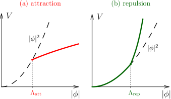
Recall, however, that the soliton parameters $\varphi_{0}$ and $R$ are related by the field equations which involve the scalar potential $V(\varphi_{0})$. We therefore consider two options. First, one can assume that the potential grows almost quadratically at weak fields, $V\sim m^{2}|\phi|^{2}$, and then flattens out beyond some scale $\Lambda_{\mathrm{att}}$ like $V\propto|\phi|^{\alpha}$ with $\alpha<2$, see Fig. 1(a). This case corresponds to particle attraction inside the solitonic core, as the energy per unit charge is smaller than the particle mass. At strong fields we approximate,

$$V\approx m^{2}|\phi|^{\alpha}\;\Lambda_{\mathrm{att}}^{2-\alpha}\qquad\mbox{at}\qquad|\phi|\gtrsim\Lambda_{\mathrm{att}}\,,$$ (13)

where $0<\alpha<2$. It is precisely the scalar self–interaction that holds the soliton — the Coleman’s Q–ball Coleman (1985) — together, since gravity is weaker: $\Lambda_{\mathrm{att}}\ll M_{pl}$ according to Eq. (10). In the field equation, the self–attraction is balanced by the kinetic pressure: $\partial_{i}^{2}\phi\sim V^{\prime}\sim\omega^{2}\phi$, or

$$\varphi_{0}/R^{2}\sim m^{2}\varphi_{0}^{\alpha-1}\;\Lambda_{\mathrm{att}}^{2-\alpha}\sim\omega^{2}\varphi_{0}\,,$$ (14)

see Appendix A for details. This gives $\omega\sim R^{-1}$,

$$N\sim(R\Lambda_{\mathrm{att}})^{2}(Rm)^{4/(2-\alpha)}\;,\;\;\;\;\mbox{and}\;\;\;\;M\sim N/R\,,$$ (15)

where we parametrize the soliton configurations with their sizes $R$.

The soliton collapses gravitationally when its compactness $R_{g}/R=2M/(M_{pl}^{2}R)$ becomes of order one, i.e. at masses above critical,

$$M_{cr}\approx RM_{pl}^{2}/2\sim\omega N_{cr}\,.$$ (16)

Substituting this relation into Eq. (15), we obtain the number of DM particles needed for collapse,

$$N_{cr}\sim\frac{M_{pl}^{2}}{m^{2}}\,\left(\frac{M_{pl}}{\Lambda_{\mathrm{att}}}\right)^{2-\alpha}\quad\mbox{for}\;\;0<\alpha<2\,.$$ (17)

At the critical point, the field inside the soliton is Planckian: $\varphi_{0,\,cr}\sim M_{pl}$, cf. Eqs. (14), (15), and (17).

Notably, the critical multiplicity (17) is minimal at ${\alpha=2}$ when the “free bosonic” expression (2) is recovered. The other values of $\alpha<2$ are less advantageous, as $\Lambda_{\mathrm{att}}$ is parametrically below the Planck scale. One obtains almost the “fermionic” multiplicity (1) in the case $V\propto|\phi|$ and even larger $N_{cr}$ for the $\phi$–independent potential. Thus, contrary to naive expectations particle attraction obstructs collapse, the reason being that the energy per particle $\omega$ becomes much smaller than $m$.

One can push the above “attractive” option to the extreme assuming that the scalar potential $V(\phi)$ decreases at strong fields, e.g. $V\propto-|\phi|^{\alpha}$. However, that would destabilize the soliton making its field evolve towards lower $V$, cf. Zakharov and Kuznetsov (2012); Levkov et al. (2017a). With no new positive terms in the potential to stop the process, the region with $V(\phi)<0$ would be eventually reached Panin and Smolyakov (2019); then the soliton turns into an expanding and Universe–destroying bubble of true vacuum Coleman (1979). Even if the bubble can be somehow forced to collapse gravitationally, the region in its center still breaks the positivity conditions, so that a naked singularity may appear instead of a black hole. If, alternatively, the potential starts growing at larger fields, again, the field stops rolling at that point, thus bringing us back to the two options in Fig. 1.

Equation (17) hints at the possibility that the second option of repulsive self–interactions with $\alpha>2$ may be more interesting, see Fig. 1(b). In this case the only attractive force is gravity. The respective soliton is called a Bose star Ruffini and Bonazzola (1969); Tkachev (1986), since it is bound by gravitational attraction compensating interaction pressure of Bose particles inside it. Note that the repulsive energy gives a subdominant contribution to the mass of the subcritical object because its opponent — the gravitational energy — remains small until the rim of collapse. We therefore keep two terms in the potential,

$$V\approx m^{2}|\phi|^{2}+m^{2}|\phi|^{\alpha}\;\Lambda_{\mathrm{rep}}^{2-\alpha}\,,$$ (18)

where now $\alpha>2$, the field $\phi$ is arbitrary, and $\Lambda_{\mathrm{rep}}$ satisfies Eq. (10). Performing the estimates similar to the ones before Ho et al. , we find out that the Bose star collapses gravitationally only at $\alpha>8/3$, see Appendix A for details. In this case the soliton field indeed gets stuck in the region of subdominant self–interactions ${\varphi_{0}\lesssim\Lambda_{\mathrm{rep}}}$ until the collapse, at which point $\varphi_{0,\,cr}\sim\Lambda_{\mathrm{rep}}$ and the soliton charge equals

$$N_{cr}\sim\frac{M_{pl}^{3}}{\Lambda_{\mathrm{rep}}m^{2}}\qquad\mbox{for $\alpha>8/3$}\,.$$ (19)

Notably, this critical multiplicity is independent of $\alpha$, see also Refs. Colpi et al. (1986) and Ho et al. . At $\Lambda_{rep}\sim m$ the expression (19) reproduces the fermionic result (1). The way to decrease the multiplicity is to increase $\Lambda_{\mathrm{rep}}$ suppressing the self–repulsion. At $\Lambda_{\mathrm{rep}}\sim M_{pl}$ that force is as weak as gravity, the field inside the critical Bose star is Planckian, and we obtain the “free bosonic” formula (2), again.

The remaining region $2<\alpha<8/3$ is worst of them all, since in that case the Bose–Einstein condensate does not clump under self–gravity. Indeed, an estimate of Appendix A shows that the self–repulsion $|\phi|^{\alpha}$ with $\alpha$ in this range is stronger than gravity at large distances. It makes the DM condensate spread over the entire volume available inside the neutron star gravitational field.

We conclude that the critical particle number $N_{cr}$ is smallest in the restricted class of models with long, Planckian–size valleys ${|\phi|\lesssim M_{pl}}$ and almost quadratic potentials $V\propto|\phi|^{2}$ at their bottoms. Any interaction impedes collapse and sharply increases the critical multiplicity. In particular, self–repulsion becomes strong, almost equivalent to the Fermi pressure at large fields — hence the “fermionic” result (19). Self–attraction does not help either: it provides negative binding energy and lowers the soliton mass which is bad for collapse. The respective critical particle number is also parametrically larger, see Eq. (17).

In the optimal model with exactly quadratic potential, the kinetic pressure inside the Bose star is compensated by the gravitational attraction Kaup (1968); Ruffini and Bonazzola (1969); Schunck and Mielke (2003). The respective object becomes gravitationally unstable at $\varphi_{0,\,cr}\sim M_{pl}$. It has the critical multiplicity Kaup (1968)

$$N_{cr}\approx 0.653\,M_{pl}^{2}/m^{2}\qquad\mbox{for $\alpha=2$}\,.$$ (20)

This result agrees with the estimate in Eq. (2). Nonrelativistic approximation remains valid during the most part of the Bose star growth and gets marginally broken at the rim of collapse.

III.2 Obstruction by quantum corrections

How far the DM model can deviate from the free bosonic theory? To find out, we require that the critical multiplicity for collapse $N_{cr}$ does not exceed the maximal amount (6) of captured DM: ${mN_{cr}\lesssim M_{\rm tot}^{\mathrm{dwarf}}}$.

In the attractive case, this condition bounds from below the scale $|\phi|\sim\Lambda_{\mathrm{att}}$ at which the scalar potential flattens out in Fig. 1(a):

$$\Lambda_{\mathrm{att}}\gtrsim M_{pl}\left(\frac{2\times 10^{-9}\;{\rm GeV}}{f\;m}\right)^{1/(2-\alpha)}\!\!\!\!,$$ (21)

see Eqs. (6), (17) and recall that $0<\alpha<2$. Typically, $\Lambda_{\mathrm{att}}$ is very large. Indeed, since the critical Q–ball has $\varphi_{0}\sim M_{pl}$, the model with flat potential should be trustable, i.e. renormalizable and weakly coupled, all the way up to the Planckian scale. The only manifestly renormalizable flat potential is $V=\mathrm{const}$, it appears Levkov et al. (2017b) e.g. in the celebrated Friedberg–Lee–Sirlin model Friedberg et al. (1976). In this case

$$\Lambda_{\mathrm{att}}\gtrsim 5\times 10^{13}\;\mbox{GeV}\;(mf/100\,\mathrm{GeV})^{-1/2}\;,\;\;\alpha=0\,.$$ (22)

Soon we will see that large scales (21), (22) are problematic because multiloop corrections to the scalar potential become relevant at $\varphi_{0}\ll\Lambda_{\mathrm{att}}$. They generate interaction pressure and prevent collapse.

The scale $\Lambda_{\mathrm{att}}$ can be substantially lowered in a specific class of renormalizable multifield models where the potentials at the bottoms of curved valleys have ${\alpha\approx 2}$. We will consider this option in Sec. IV.

In the opposite, self–repulsive case the inequality $mN_{cr}\lesssim M_{\rm tot}^{\mathrm{dwarf}}$ also provides a large scale

$$\Lambda_{\mathrm{rep}}\gtrsim 2\times 10^{8}\;\mbox{GeV}\;(mf/100\,\mathrm{GeV})^{-1}\,,$$ (23)

following from Eqs. (6) and (19). This condition strongly suppresses all repulsive self–interactions at fields ${|\phi|\lesssim\Lambda_{\mathrm{rep}}}$, see Eq. (18). For example, in the $\lambda_{4}|\phi|^{4}/4$ case,

$$\lambda_{4}\equiv(2m/\Lambda_{\mathrm{rep}})^{2}\lesssim 7\times 10^{-13}f^{2}(m/100\,\mathrm{GeV})^{4}\,.$$ (24)

It is worth remarking that the renormalizability of the repulsive potential is not required, since the Bose star field ${\varphi_{0}\lesssim\Lambda_{\mathrm{rep}}}$ remains parametrically below the natural cutoff of the theory (18) prior to collapse.

Now, recall that our dark matter should interact with the visible sector, and strongly enough, in order to be captured by the neutron star. The respective couplings should be renormalizable and stay under control at strong fields — hence, their forms are constrained by the Standard Model symmetries. Let us demonstrate that, generically, loop corrections from these interactions break the desired properties of the dark matter potential: lift its flat parts and generate unacceptably large repulsive vertices, as has been first pointed out in Bell et al. (2013).

Figure 2: Scattering $\phi n\to\phi n$.

Couple, e.g., the field $\phi$ to the Higgs doublet $H(x)$ by deforming the potential of the latter to

$$V=\lambda_{H}\left(H^{\dagger}H-\frac{v^{2}}{2}-\frac{y|\phi|^{2}}{2\lambda_{H}}\right)^{2}+m^{2}|\phi|^{2}\,,$$ (25)

cf. Shaposhnikov and Tkachev (2006); Bezrukov and Gorbunov (2010). Here $v\approx 246\,\mbox{GeV}$ and ${\lambda_{H}\approx 0.13}$ are the standard Higgs parameters, and the new constant $y$ regulates its interactions with the dark sector. Notably, the model is weakly coupled at ${y\ll(4\pi\lambda_{H})^{1/2}\sim 1}$.

The physical Higgs field $h(x)$ is defined as ${H^{\dagger}H=(v+h)^{2}/2}$. It interacts with neutrons $n$ via the effective Yukawa vertex ${V_{hnn}\approx 2m_{n}h\bar{n}n/(9v)}$ which is known up to light quark contributions giving a factor $1\div 2$ Shifman et al. (1978); Cirelli et al. (2013); $m_{n}\approx\mbox{GeV}$ is the neutron mass. This means that the dark matter also scatters off neutrons. The respective diagram is shown in Fig. 2 and the cross section at nonrelativistic momenta equals

$$\sigma=\frac{y^{2}m_{n}^{4}}{81\pi m_{H}^{4}m^{2}}\,,$$ (26)

where $m_{H}=v(2\lambda_{H})^{1/2}\approx 125\,\mbox{GeV}$. Importantly, the scattering probability ${f\equiv\sigma/\sigma_{\mathrm{crit}}<1}$ should be large enough to capture the $\phi$–particles inside the neutron star, see the constraints (21), (23). Thus, the coupling $y$ is large.

On the other hand, the same coupling (25) generates DM pressure at strong fields. In fact, we have already tuned this potential to cancel DM self–interactions at the classical level. Namely, at large fixed $\varphi_{0}=|\phi|$ the Higgs field adjusts itself to minimize the first term in Eq. (25),

$$H^{{\dagger}}H\equiv\frac{1}{2}(h+v)^{2}=\frac{v^{2}}{2}+\frac{y|\phi|^{2}}{2\lambda_{H}}\,.$$ (27)

As a consequence, the tree potential is quadratic at the bottom of this potential valley, ${V\approx m^{2}|\phi|^{2}}$. Nevertheless, the self–coupling reappears, again, once loop contributions from the visible matter are included. As an illustration, let us first ignore all fields except for the Higgs boson and $\phi$ itself. Then their one–loop effective potential Weinberg (2013) at large $|\phi|\propto h$ along the valley (27) equals,

$$\Delta V_{\mathrm{1-loop}}\approx\lambda_{4,\,\mathrm{eff}}\,|\phi|^{4}/4\,.$$ (28)

where $\lambda_{4,\,\mathrm{eff}}=y^{2}L/(2\pi^{2})+O(y^{3}/\lambda_{H})$ is a correction to the $|\phi|^{4}$ self–coupling, ${L=\ln(|\phi|/\Lambda_{\mathrm{ren}})}$, and ${\Lambda_{\mathrm{ren}}\sim m}$ is a renormalization scale. Note that a proper calculation of the effective potential at strong fields includes renormalization group resummation of the leading logs Bednyakov et al. (2013); Chetyrkin and Zoller (2013). However, that usually introduces an order–one factor in $\lambda_{4,\,\mathrm{eff}}$ which does not affect our estimates.

We see that Eq. (28) brings in the $|\phi|^{4}$ repulsion even if it was absent before. Moreover, since $\lambda_{4,\,\mathrm{eff}}$ logarithmically depends on the field, the new contribution cannot be canceled by any renormalizable counter-terms even if an arbitrarily precise fine–tuning is allowed. An obvious way out is to make the one–loop repulsion small, so that it does not preclude black hole formation. Requiring $\lambda_{4,\,\mathrm{eff}}$ to satisfy Eq. (24) with $\sigma$ given by Eq. (26), we obtain the inequality

$$y\gtrsim 400\,L^{1/2}>400\,,$$ (29)

which cannot be satisfied in a weakly coupled model with $y\ll 1$. Moreover, even this unacceptable lower limit can be achieved only if $m\gtrsim{\rm PeV}$. We conclude that either the coupling constant $y$ is too small for accumulating the required amount of $\phi$–particles, or the interaction pressure caused by the same constant prevents the $\phi$–condensate from collapsing.

As an alternative, one may try to couple $\phi$ to fermions that generate negative terms in the effective potential. In the model (25) this amounts to recalling that every massive Standard Model field gives a potential to Higgs and therefore produces a vertex $|\phi|^{4}\propto h^{4}$ along the valley (27). The leading contribution is negative and comes from the top quark Yukawa coupling $y_{t}\approx 1$. We obtain $\delta\lambda_{4,\,\mathrm{eff}}=-3y^{2}y_{t}^{2}L/(8\pi^{2}\lambda_{H}^{2})$. This definitely destabilizes the valley Buttazzo et al. (2013); Bednyakov et al. (2015) unless even larger positive $|\phi|^{4}$ terms are introduced, which, however, returns us to the no–go estimates given above.

Somewhat more elegantly, one may organize a (partial) cancellation between the fermionic and bosonic loops. But that would mean upgrading the Standard Model to (N)MSSM. In that case the inequality $mN_{cr}\lesssim M_{\rm tot}^{\mathrm{dwarf}}$ imposes strong constraints on the supersymmetry–breaking operators that detune the cancellation Bell et al. (2013). In Sec. IV we consider more economic and general possibility.

To sum up, loop corrections from the visible sector are dangerous, generic, and cannot be avoided. Thus, we need a special mechanism to tame them.

III.3 Requirements for the DM model

Let us summarize the properties of dark matter model needed for black hole formation inside the neutron star.

(a) The scalar potential of the model should include a long valley parametrized by the complex scalar $\phi$. The valley should extend to large fields: to $|\phi|\sim M_{pl}$ in the case of attractive self–interactions (13) or, in the repulsive case (18), at least to the scale ${|\phi|\sim\Lambda_{\mathrm{rep}}}$ given in Eq. (23). The model should remain weakly coupled at these fields i.e. be renormalizable or have a sufficiently high cutoff.

(b) The potential should be almost quadratic along the valley, ${V\approx m^{2}|\phi|^{2}}$. All its repulsive terms should be suppressed at least by the scale $\Lambda_{\mathrm{rep}}$ in Eqs. (18), (23). The potential may become flatter than quadratic (attractive) inside finite $\phi$ intervals, but that should not ruin its renormalizability or destabilize the vacuum. If the potential becomes attractive asymptotically at ${|\phi|\gtrsim\Lambda_{\mathrm{att}}}$, like in Eq. (13), the scale $\Lambda_{\mathrm{att}}$ should be sufficiently high, see Eq. (21).

(c) Quantum corrections from the dark matter and visible sectors should not destabilize the valley or create effective interactions breaking the condition (b).

We have already demonstrated that the condition (c) is usually violated by dark matter interactions with the visible sector in one–field DM models. We now turn to models where this can be avoided.

IV Models with bended valleys

IV.1 The mechanism

Start from the arbitrary model for the DM field $\phi$ and add the second complex scalar $\chi$ in such a way that $\phi$ and $\chi$ have global charges 1 and 2, respectively. The coupling between the two is then chosen in a specific renormalizable and positive–definite form,

$$V=\lambda\left|\phi^{2}-\Lambda\chi\right|^{2}+m^{2}|\phi|^{2}+\lambda^{\prime}\,|\phi|^{4}/4\,,$$ (30)

where the last two terms represent the original $\phi$ potential. This model is invariant under phase rotations ${\phi\to\mathrm{e}^{i\theta}\phi}$ and $\chi\to\mathrm{e}^{2i\theta}\chi$. In the vacuum $\phi=\chi=0$ all fields are massive: ${m_{\phi}=m}$ and ${m_{\chi}=\Lambda\lambda^{1/2}}$. We will assume that the first term in the potential is the largest:

$$m\ll\Lambda\lambda^{1/2}\qquad\mbox{and}\qquad\lambda^{\prime}\ll\lambda\,.$$ (31)

This means, in particular, that the $\chi$–particles are heavy and do not change cosmology.

The trick of the new model is to make the potential valley bend in the $\phi$—$\chi$ space. Indeed, the low–energy field configurations are expected to minimize the largest term in Eq. (30), i.e. satisfy

$$\chi=\phi^{2}/\Lambda\,.$$ (32)

The other terms of $V$ create a small potential along this valley. The same is true, in particular, for the stationary nonrelativistic soliton,

$$\phi=\varphi(\bm{x})\,\mathrm{e}^{-i\omega t}\;,\qquad\chi=\tilde{\chi}(\bm{x})\,\mathrm{e}^{-2i\omega t}\,,$$ (33)

which has real profiles $\varphi$, $\tilde{\chi}$ satisfying Eq. (32).

Let us explicitly demonstrate that the valley extends in the $\phi$ direction at small fields, then takes a turn at ${\phi\sim\chi\sim\Lambda}$ and goes along $\chi$. To this end we introduce a combination $\rho(\bm{x})$ of the solitonic profiles which has a canonical kinetic term along the valley: $(\partial_{i}\rho)^{2}=(\partial_{i}\varphi)^{2}+(\partial_{i}\tilde{\chi})^{2}$. Using Eq. (32) and integrating, we find

$$\rho(\varphi)=\frac{\varphi}{2}\sqrt{1+\frac{4\varphi^{2}}{\Lambda^{2}}}+\frac{\Lambda}{4}\,\mathrm{arcsinh}\left(\frac{2\varphi}{\Lambda}\right)\,.$$ (34)

The classical potential $V(\rho)$ at the bottom of the valley is obtained by inverting Eq. (34) and substituting $\varphi(\rho)$ into the last two terms of Eq. (30).

At small fields we get $\rho\approx\varphi$; hence, the valley stretches in the $\phi$ direction, indeed. Taylor series expansion in $\rho/\Lambda\ll 1$ then gives a nonlinear valley potential,

$$V(\rho)=m^{2}\rho^{2}+\lambda_{\rho}\rho^{4}/4+O(\rho^{6}/\Lambda^{4})$$ (35)

with ${\lambda_{\rho}=\lambda^{\prime}-16m^{2}/(3\Lambda^{2})}$. We have already discussed in Sec. III that the $\rho^{4}$ term cannot be large positive, or it would stop the soliton from growing. Requiring

$$\lambda^{\prime}/4=\beta(m/\Lambda)^{2}\;,\qquad\beta\lesssim 1\,,$$ (36)

we ensure that the effective coupling is attractive at small fields: ${\lambda_{\rho}<0}$. This is not dangerous for vacuum stability, since the overall potential of our model is explicitly positive–definite.

The region $\phi\gg\Lambda$ is entirely different. Expression (34) gives $\rho\approx\varphi^{2}/\Lambda$ meaning that the valley runs along $\tilde{\chi}\approx\rho$. At the same time, the potential at the bottom of the valley is quadratic: ${V(\rho)=\mu^{2}\rho^{2}+}(\mbox{smaller terms})$, where we denoted

$$\mu=m\beta^{1/2}\lesssim m\,,$$ (37)

and used Eqs. (30), (36). So, quartic self–interaction in this part of the valley is absent, and the effective $\rho$ mass is smaller than $m$.

Now we see how the bended valley (32) works. Originally, the model (30) includes the term $\lambda^{\prime}|\phi|^{4}$ creating pressure. The same term, however, reduces to a mass $|\phi|^{4}\propto|\chi|^{2}$ once the valley takes a turn. Moreover, this property is valid even at the quantum level.

Indeed, an explicit one–loop calculation Weinberg (2013) gives quartic effective potential at large fields: $\Delta V_{\mathrm{1-loop}}\approx\lambda_{4,\,\mathrm{eff}}\;|\phi|^{4}/4+O(\phi^{2})$ with

$$\lambda_{4,\,\mathrm{eff}}=\frac{2}{\pi^{2}}(2\lambda^{2}+\lambda\lambda^{\prime}+5\lambda^{\prime 2}/32)\,\ln\frac{|\phi|}{\Lambda_{\mathrm{ren}}}\;.$$ (38)

Thus, quantum fluctuations of $\phi$ and $\chi$ somewhat increase the constant ${\lambda^{\prime}\to\lambda^{\prime}+\lambda_{4,\,\mathrm{eff}}}$ in front of ${|\phi|^{4}\propto|\chi|^{2}}$, but do not prevent the Bose star from growing if Eq. (36) remains satisfied:

$$\lambda^{\prime}+\lambda_{4,\mathrm{eff}}<4(m/\Lambda)^{2}\,.$$ (39)

The latter inequality is easily met if $\Lambda$ is not too far away from $m$.

One may wonder, why the dangerous terms $\Delta V=c_{1}|\phi\chi|^{2}+c_{2}|\chi|^{4}$ are not generated at the one–loop level. If present, they would create an undesired pressure inside the strong–field soliton. However, the auxiliary field $\chi$ enters the interaction potential in the combination $\Lambda\chi$, where $\Lambda$ has mass dimension 1. On dimensional grounds, $c_{2}\sim c_{1}^{2}\sim(\Lambda/\Lambda_{\mathrm{cutoff}})^{4}$, where $\Lambda_{\mathrm{cutoff}}$ is a cutoff for loops. Thus, the multiloop diagrams for the dangerous terms converge, the constants $c_{1}$, $c_{2}$ do not depend logarithmically on the fields, and one can tune them to zero at $\phi,\,\chi\gg\Lambda$. Barring this fine–tuning, the quantum corrections are harmless in the model (30).

Let us visualize the growth of the Bose–Einstein condensate in the model of this Section. Initially, it forms a Bose star held by the gravitational forces. This object becomes denser with time due to continuous inflow of dark matter particles. At ${\rho\sim m^{2}/(|\lambda_{\rho}|M_{pl})\ll\Lambda}$ the $\lambda_{\rho}\rho^{4}$ self–attraction overcomes the kinetic pressure, and the Bose star collapses as a bosenova Zakharov and Kuznetsov (2012); Chavanis (2011). This means that its central part starts squeezing in a particular self–similar fashion Zakharov and Kuznetsov (2012); Levkov et al. (2017a) developing strong fields. The squeeze–in halts when the field in the center reaches ${\rho\sim\Lambda}$ and the valley potential stops being attractive, cf. Eby et al. (2016a); Levkov et al. (2017a).

This is the moment when a droplet of much denser condensate with $\rho\sim\chi\gtrsim\Lambda$ appears in the Bose star center. At first, it has the field strength $\chi\sim\Lambda$. However, the droplet is expected to grow in density towards $\chi\gg\Lambda$ as more $\chi$–particles join in. Indeed, once it is there, a condensation process $\phi\phi\to\chi$ with energy release $2m-\mu$ becomes allowed. Even if one assumes that this direct process is ineffective dynamically, the condensation should continue in other, recurrent way. Without direct transmutation into $\chi$, the $\phi$ particles would create another dilute Bose star around the $\chi$–droplet, and that star would collapse, again, feeding the droplet. In any case all global charge should be eventually transported into the dense $\chi$–cloud and may never leave it due to large binding energy $2m-\mu$ of the $\chi$ particles, cf. Eq. (37).

Notably, we expect that the central $\chi$–cloud quickly thermalizes into a dense and non–interacting Bose star with $\chi\gg\Lambda$. Indeed, the $\chi$–particles effectively scatter with self–coupling $\gtrsim\lambda^{\prime}$ at the cloud boundaries. In there, ${\chi\sim\Lambda}$ and hence the particle number density is huge: $n\sim\mu\Lambda^{2}$. A conservative estimate constrains the relaxation time from the above Zakharov et al. (1992); Semikoz and Tkachev (1995); Levkov et al. (2018),

$$\tau_{\chi}\sim(\xi\sigma_{\phi\phi}v_{\chi}nf)^{-1}\ll 40\,\mbox{yr}\;v_{\chi}^{2}\;\frac{(100\,\mathrm{GeV})^{3}}{\mu\Lambda^{2}}\,,$$ (40)

where $\xi\gg(\Lambda/M_{pl})^{2}$ is the time fraction spent by the particles at the cloud periphery, $\sigma_{\phi\phi}\gtrsim\lambda^{\prime 2}/(64\pi\mu^{2})$ is their cross section, $f\propto n/(\mu v_{\chi})^{3}$ is the phase–space density, $v_{\chi}$ is velocity, and we used Eqs. (36), (37). Even the most conservative choices of parameters give small $\tau_{\chi}$ compared to the lifetime of the Universe – thus, the relaxation is effective, indeed.

Now, we recall that the self–interactions are absent at ${\chi\gg\Lambda}$. This means that the respective Bose star will grow pressureless until it collapses gravitationally into a black hole. The latter event requires the critical charge

$$N_{cr}\approx 1.3\,M_{pl}^{2}/(\beta m^{2})\,,$$ (41)

where the numerical coefficient is larger by a factor $2/\beta$ than in Eq. (20) because $\chi\sim\rho$ has global charge 2 and mass ${\mu=m\beta^{1/2}}$.

We thus constructed a model with almost an optimal critical multiplicity for the collapse of Bose–Einstein condensate into a black hole. In the next Section we will see that interaction with the visible sector and hence DM capture can be added to this model without disrupting the picture.

IV.2 Adding interactions with the visible sector

We couple the DM field to the Higgs doublet in the same way as before — by adding the first term in Eq. (25) to the scalar potential (30). This makes the $\phi$–particles scatter off neutrons with the cross section $\sigma\propto y^{2}$ in Eq. (26). Importantly, we leave $\chi$ to interact only with $\phi$. This maintains the desired properties of the strong–field Bose stars in our model.

Now, the Higgs field changes along the potential valley (32) according to Eq. (27). As a consequence, a nonzero Higgs profile $h(\bm{x})$ is generated inside every stationary soliton. A combination of the three profiles — $\varphi$, $\tilde{\chi}$, and $h$ — with the canonical kinetic term is

$$\rho(\varphi)=\int_{0}^{\varphi}d\varphi^{\prime}\sqrt{1+\frac{4\varphi^{\prime 2}}{\Lambda^{2}}+\frac{y^{2}\varphi^{\prime 2}}{\lambda_{H}(m_{H}^{2}+2y\varphi^{\prime 2})}}\,,$$ (42)

where the last contribution comes from the Higgs field.

Notably, with interactions (25) included, the effect of the bended valley remains essentially the same. Indeed, $\rho$ is still proportional to $\varphi$ and $\tilde{\chi}$ at $\rho\ll\Lambda$ and $\rho\gg\Lambda$, respectively. In the weak–field regime $\rho\lesssim\Lambda$ the valley potential is nonlinear, Eq. (35), and has almost the same quartic constant $\lambda_{\rho}$ as before. We therefore again impose the condition (36) to make $\lambda_{\rho}$ negative at weak fields. Once the valley turns at $\rho\gg\Lambda$, the potential $V(\rho)$ becomes quadratic with mass (37), as guaranteed by the mechanism of the previous Section.

All these nice properties remain valid because $\chi$ does not couple directly to the Standard Model fields and still enters the overall potential in the combination $\Lambda\chi$ with dimensionful $\Lambda$. This makes the nonlinear interactions vanish in the strong–field region, and they cannot be generated by loops. We check the latter property by computing the one–loop effective potential in the three–field model of $\phi$, $\chi$, and $H$ at the bottom of the valley (27), (32). The result at large fields is given by Eq. (28), where the constant $\lambda_{4,\,\mathrm{eff}}$ equals Eq. (38) plus the Higgs contribution

$$\delta\lambda_{4,\,\mathrm{eff}}=\frac{y^{2}}{\pi^{2}\lambda_{H}}\!\left(\lambda+\frac{\lambda_{H}}{2}+\frac{y}{2}+\frac{3\lambda^{\prime}}{8}+\frac{y^{2}}{8\lambda_{H}}\right)\ln\frac{|\phi|}{\Lambda_{\mathrm{ren}}}\,.$$

Similarly, the other Standard Model fields are expected to generate $\Delta V_{\mathrm{1-loop}}\propto h^{4}\propto|\phi|^{4}$. Regardless of the value of $\lambda_{4,\,\mathrm{eff}}$, the loop corrections safely change the mass $|\phi|^{4}\propto|\chi|^{2}$ in the strong–field region. The value of $\mu$ then can be made positive by adjusting $\lambda^{\prime}$. For simplicity we assume below that the loop corrections are small compared to $\lambda^{\prime}$.

Without the interaction pressure, the strong–field Bose star collapses gravitationally at almost optimal critical charge (41). This value cannot exceed the total number of captured dark matter particles, $M_{\rm tot}^{\mathrm{(dwarf)}}/m>N_{cr}$. One obtains the inequality

$$y>10^{-7}\,\left(m\over 100\,\mbox{GeV}\right)^{1/2}\beta^{-1/2}$$ (43)

using Eqs. (6), (26), and (41). This constraint is relatively mild and can be easily satisfied.

Indeed, let us show that a viable parametric region for our model can be selected. One starts by specifying $m$ within the WIMP mass range and $\beta\lesssim 1$. The coupling constant $y$ is then chosen to satisfy Eq. (43) together with the constraints from the DM detection experiments. Below we will argue that a narrower region

$$2\times 10^{-6}\lesssim y\;\left(m\over 100\,\mbox{GeV}\right)^{-1/2}\lesssim 2\times 10^{-5}\,\beta^{-1/2}$$ (44)

is better for phenomenology. The next parameters are $\lambda$ and $\lambda^{\prime}\ll\lambda$. In the simplest case one takes ${\lambda\sim y/\lambda_{H}^{1/2}}$ and $\lambda^{\prime}\gtrsim\lambda^{2}$, thus suppressing the running of $\lambda^{\prime}$: $\lambda_{4,\,\mathrm{eff}}$, $\delta\lambda_{4,\,\mathrm{eff}}\lesssim\lambda^{\prime}$. Finally, the scale $\Lambda$ is given by Eq. (36). We conclude that all the constraints can be satisfied if the hierarchy

$$\lambda^{\prime}\sim\lambda^{2}\sim y^{2}/\lambda_{H}\;,\qquad\Lambda\sim m/\lambda\;,\qquad\beta\lesssim 1$$ (45)

is valid and $y$ belongs to the interval (44).

IV.3 Generalizations

So far we relied on fine–tuning to kill the $|\phi\chi|^{2}$ and $|\chi|^{4}$ terms in the potential. If added, these interactions should be extremely weak — say, the operator $\lambda_{2}^{\prime}|\chi|^{4}/4$ should satisfy the analog of Eq. (24):

$$\lambda_{2}^{\prime}\lesssim 2\times 10^{-13}\,f^{2}\beta^{3}\left(m/100\,\mbox{GeV}\right)^{4}\,.$$

Can we allow stronger interactions at $|\chi|\gtrsim\Lambda$?

The answer is yes, if extra auxiliary scalars are introduced. Namely, let us add the $|\chi|^{4}$ term along with the new field $\chi_{2}$ that has a global charge 4. The new terms in the potential are

$$V_{2}=\lambda_{2}|\chi^{2}-\Lambda_{2}\chi_{2}|^{2}+\lambda^{\prime}_{2}|\chi|^{4}/4\,,$$ (46)

where $\lambda_{2}^{\prime}=4\beta_{2}(\mu/\Lambda_{2})^{2}$ and $\beta_{2}\lesssim 1$; cf. Eq. (36). Now, the valley takes a second turn at ${\chi\sim\chi_{2}\sim\Lambda_{2}}$, before the $|\chi|^{4}$ interaction becomes relevant.

One can continue this procedure and arrive at the “clockwork–like” model with $n$ fields $\chi_{i}$, a hierarchy of scales $\Lambda\ll\Lambda_{2}\ll\dots\ll\Lambda_{n}$, masses at strong fields ${\mu_{i}=\mu_{i-1}\beta_{i}^{1/2}}$, and many coupling constants ${\lambda_{i}^{\prime}\equiv(2\mu_{i}/\Lambda_{i})^{2}}$, where $\beta_{i}\lesssim 1$. The Bose star made of the last field $\chi_{n}$ collapses gravitationally at the critical charge

$$N_{cr}=(M_{pl}/m)^{2}\prod_{i=1}^{n}(2/\beta_{i})\,.$$ (47)

If $n\sim O(1)$, this multiplicity is not exceedingly large.

Of course, the field $\chi$ can be made interacting in other, old–fashioned ways — say, by supersymmetry. To this end one upgrades this field to the supersymmetric sector with a flat direction Gherghetta et al. (1996) which represents the $|\chi|\gtrsim\Lambda$ part of the valley. The flat direction should be lifted by soft terms giving the mass to the condensate. Then the superpotential will be protected from quantum corrections as long as its fields couple to the visible matter via the dimensionful constant $\Lambda$.

V Conclusions

We considered formation of black holes with masses ${\approx 1\,M_{\odot}}$ by means of bosonic dark matter collapse inside neutron stars. This scenario includes DM capture by the neutron stars, its thermalization with neutrons, Bose–Einstein condensation, and at last — gravitational collapse into seed black holes which eventually consume the stars. The overall process includes two conflicting requirements on the DM model Bell et al. (2013). On the one hand, the DM can be captured only if it interacts strongly enough with the visible sector. On the other hand, loop contributions of the same interactions generate DM self–couplings and hence pressure inside dense DM clouds, impeding their collapse. We have found, in agreement with Ref. Bell et al. (2013), that the conflict cannot be resolved by tuning the parameters of the single–field DM models, neither can it be achieved by optimization of their scalar potentials.

Using the crucial observation that the conflicting requirements are imposed at different scales, we proposed a mechanism that enables black hole formation within this scenario. The respective DM models are deformed at strong fields, i.e. in the regions inaccessible to the direct experiments. Their scalar potentials include bended valleys that go along the dark matter scalar $\phi$ at $|\phi|\lesssim\Lambda$ and then turn in the direction of a new field $\chi$. In this case $\chi$ self–pressure can be made small and, notably, can be protected from all quantum corrections by super–renormalizable couplings to other fields, supersymmetry, or a “clockwork–like” mechanism. As a consequence, the growth of the DM cloud inside the neutron star includes a phase transition $\phi\phi\to\chi$ at a certain density followed by the gravitational collapse of the pressureless $\chi$ condensate.

In our model formation of a black hole requires a relatively small number Eq. (41) of DM particles which can be accumulated inside the neutron star even at extremely weak couplings, see e.g. Eq. (43) in the case of interaction (25). However, other conditions become relevant at this point. First, the newborn seed black hole cannot be too light, $M_{\mathrm{BH}}\gtrsim 10^{13}\,\mbox{g}$, or it evaporates faster than it accretes neutrons Kouvaris and Tinyakov (2011b). In our model $M_{\mathrm{BH}}\approx\mu N_{cr}/2$, so this condition constrains an effective mass $\mu$ of the auxiliary scalar $\chi$ at strong fields,

$$\mu\equiv m\beta^{1/2}\lesssim 17\;\mbox{GeV}\,,$$ (48)

where Eq. (41) was used, $m$ is the mass of the DM particles, and $\beta\lesssim 1$ parametrizes their self–interactions via Eq. (36). Taking sufficiently small $\beta$, one fulfills Eq. (48) in the entire WIMP mass range.

Second, thermalization of DM with neutrons is an obligatory part of our scenario needed to form a dense central cloud. But at weak couplings the equilibrium may be unachievable even on the cosmological timescales, since DM interactions with neutrons are further suppressed at low energies by Pauli blocking Goldman and Nussinov (1989). For scalar vertices, the respective thermalization time was estimated in Garani et al. (2021) as $\tau_{\mathrm{NS}}\approx 35\pi^{2}/(12\sigma mT^{2})$, where ${T\sim 10^{5}\,\mbox{K}}$ is the neutron star temperature and $\sigma$ is the DM–neutron cross section in vacuum, Eq. (26). Requiring ${\tau_{\mathrm{NS}}\lesssim 10^{10}}$ yr, we constrain the coupling constant,

$$y\gtrsim 2\times 10^{-6}\,\left(m\over 100\,\mbox{GeV}\right)^{1/2}\,.$$ (49)

This condition is marginally stronger than Eq. (43) needed for capture.

Third and finally, our mechanism should not be too efficient in turning all neutron stars into solar–mass black holes — after all, thousands of neutron stars are observed in our Galaxy. One way to suppress their transmutation is to make the DM–neutron coupling moderately small, so that only the densest DM environments would allow the stars to accumulate the critical mass for collapse. Using the Milky Way parameters, we require ${M_{\rm tot}^{\mathrm{MW}}\lesssim mN_{cr}}$ or

$$y\lesssim 2\times 10^{-5}\;\left(m\over 100\,\mbox{GeV}\right)^{1/2}\,\beta^{-1/2}\,,$$ (50)

where Eqs. (5), (26), and (41) were used. Note that Eq. (50) is not far from the conditions (43), (49); this is due to the fact that the DM parameters vary by only a few orders of magnitude from galaxy to galaxy.

It is worth noting that we have disregarded several points which are important for the scenario of this paper. First, it is crucial that the DM is non–annihilating and satisfies constraints coming from its generation in the early Universe and from the DM detection experiments. It remains to be seen if all these conditions can be fitted together with the requirements of our mechanism.

Second, we have not analyzed the astrophysical signatures of the neutron stars converting into the solar–mass black holes. In our scenario, the transmutation is controlled by a single parameter — the number of DM particles $N_{cr}$ required for collapse. Thus, regardless of the underlying DM model the neutron stars will be converted in the parts of the Universe where the DM abundance and velocity ensure its efficient accumulation. As a consequence, solar–mass black holes will be distributed in a specific way among the galaxies of different types. For example, a discovery of old neutron stars in the dwarf galaxies — the best–known environments for the DM accumulation — would exclude a sizable overall abundance of the transmuted neutron stars in the Universe.

Third, several parts of our mechanism deserve a detailed numerical study. We expect that the phase transition of the DM particles into the $\chi$ quanta proceeds in a spectacular first–order way, starting as a self–similar bosenova collapse Zakharov and Kuznetsov (2012); Levkov et al. (2017a) and ending up with formation of a dense $\chi$ condensate. This full two–stage proscess has never been simulated before; in the main text we have just crudely estimated the time of $\chi$ condensation to be small, see Eq. (40). The other unexplored subject is the growth of the $\chi$ Bose–Einstein condensate in the end of the process. We assumed that the growth continues even when the condensate becomes incredibly small in size. On the one hand, this optimism is based on the fact that unlike in Refs. Levkov et al. (2018); Eggemeier and Niemeyer (2019); Chen et al. (2020, 2021), the DM interactions in our model are short–range. On the other hand, even in the worst case the growth of the $\chi$–condensate may proceed in a recurring indirect way: by growing the $\phi$ condensate via thermalization to the point when the transition $\phi\phi\to\chi$ happens, and then growing the $\phi$ condensate, again. The details of this process also should be studied numerically.

Fourth, although viability of our new mechanism does not depend on the details of dark matter capture and thermalization, its predictions in a particular model rely on a quantitative description of these phenomena. Thus, precise identification of a phenomenologically acceptable parameter region for the dark matter model should include studies of astrophysical uncertainties, equation of state for the nuclear matter, and DM interactions with it. Besides, renormalization group equations should be solved for the dark matter constants $\lambda^{\prime}$ and $\lambda$ which are scale–dependent and run on par with the Standard Model couplings.

Fifth and finally, it might be interesting to explore dark matter collapse in the centers of white dwarfs within our model. Despite being more dilute than the neutron stars, the latter objects are also better understood, which makes them a perspective testing ground for dark matter studies.

In a nutshell, our study demonstrates that almost any model of bosonic DM can be modified at strong fields in such a way that the solar–mass black holes can appear by transmuting the neutron stars. This calls for a proper identification of low–mass compact objects in astrophysical observations, cf. Abbott et al. (2021e) and Abbott et al. (2021f).

Appendix A Q–ball and Bose star parameters

Here we derive parametric dependence of the soliton mass $M$ and radius $R$ on its global charge $N$ in the models of Sec. III. To this end we adopt a simple version of the variational ansatz Ho et al. ; Chavanis (2011); Eby et al. (2016b) ignoring order–one numerical coefficients wherever possible. We will separately study the solitonic Q–ball Nugaev and Shkerin (2020) stabilized by the attractive self–interactions and the gravitationally bound Bose star Visinelli in the case of self–repulsion.

Start with the Q–ball in the model (9) for the complex scalar field $\phi(x)$. We will assume that its scalar potential $V$ becomes flat, i.e. attractive, at strong fields ${|\phi|\gtrsim\Lambda_{\rm att}}$, where it can be roughly approximated as a power–law (13) with $\alpha<2$. Suppose the stationary Q–ball in this model has the form of a single bell–shaped lump with typical field strength $\varphi_{0}$ and size $R$:

$$\phi=\varphi_{0}\,f(\bm{x}/R)\,\mathrm{e}^{-i\omega t}\;,$$ (51)

where $f(\bm{y})$ is a dimensionless order–one function with the support at ${|\bm{y}|=|\bm{x}|/R\lesssim 1}$; the time dependence follows from Eq. (11).

Since the Q–ball is mostly bound by the self–attraction, we can compute its parameters in flat spacetime ignoring gravity. Substituting Eq. (51) into the energy and charge of this object, we get,

$$M\sim\omega^{2}\varphi_{0}^{2}R^{3}+\varphi_{0}^{2}R+m^{2}\varphi_{0}^{\alpha}\Lambda_{\rm att}^{2-\alpha}R^{3}\;,$$ (52)

$$N\sim\omega\varphi_{0}^{2}R^{3}\;,$$ (53)

where we omitted $\varphi_{0}$– and $R$–independent numerical coefficients of order 1 in front of every term — these come from the integrals over $\bm{y}$ of powers of $f(\bm{y})$ and its derivatives.

We now minimize $M$ with respect to $\varphi_{0}$ and $R$ at a fixed $N$. Expressing $\omega$ from Eq. (53), we substitute it into Eq. (52) and differentiate the result with respect to the unknowns. We get,

$$\varphi_{0}{\partial M\over\partial\varphi_{0}} \sim-{2N^{2}\over\varphi_{0}^{2}R^{3}}+2\varphi_{0}^{2}R+\alpha m^{2}\varphi_{0}^{\alpha}\Lambda_{\rm att}^{2-\alpha}R^{3}=0\;,$$

$$R\,{\partial M\over\partial R} \sim-{3N^{2}\over\varphi_{0}^{2}R^{3}}+\varphi_{0}^{2}R+3m^{2}\varphi_{0}^{\alpha}\Lambda_{\rm att}^{2-\alpha}R^{3}=0\;.$$

Notably, the solution of these equations does not exist at ${\alpha\geq 2}$ when self–attraction changes to self–repulsion. Away from that region, all terms in the equations are of the same order:

$$\varphi_{0}^{2-\alpha}\sim(mR)^{2}\Lambda_{\mathrm{att}}^{2-\alpha}\quad\mbox{and}\quad N\sim\varphi_{0}^{2}R^{2}\,.$$ (54)

Using Eq. (53), we find that ${\omega\sim R^{-1}}$ and reproduce Eqs. (14), (15) from the main text.

It is worth noting that $\omega\sim R^{-1}\ll m$ at sufficiently large $N$, see Eq. (15). Thus, the particles inside the large Q–ball are very light due to mass deficit. As a consequence, the overall soliton is lighter and less amenable to gravitational collapse than a collection of free particles with the same charge.

Now, consider a Bose star in the model with the scalar potential (18) and $\alpha>2$. Recall that the flat–space solution does not exist in this case — hence, we add gravitational attraction. In the stationary non–relativistic limit, this amounts to introducing the metric $g_{00}=1+2U$ and $g_{ij}=-(1-2U)\,\delta_{ij}$, where $U<0$ is a time–independent Newtonian potential, ${|U|\ll 1}$. With gravity included, the energy and charge of the nonrelativistic soliton read,

$$M=\int d^{3}\bm{x}\,\Bigl{\{}(1-4U)|\partial_{0}\phi|^{2}+|\partial_{i}\phi|^{2}+(\partial_{i}U)^{2}/(8\pi G)$$

$$\qquad\qquad\;\;+(1-2U)\,m^{2}|\phi|^{2}+m^{2}|\phi|^{\alpha}\Lambda_{\mathrm{rep}}^{2-\alpha}\Bigr{\}}\,,$$ (55)

$$N=i\int d^{3}\bm{x}\,(1-4U)(\phi^{*}\partial_{0}\phi-\phi\partial_{0}\phi^{*})\,,$$ (56)

where the last term in the first line represents the energy density of the gravitational field and we ignored the gravitational effect of the self–interaction energy ${\delta V\propto|\phi|^{\alpha}}$.

Following the same strategy as before, we assume that the solution has the form (51) characterized by the field strength $\varphi_{0}$, size $R$, and the gravitational potential in the center $U_{0}$. Omitting all order–one coefficients, again, we find,

$$M\sim(1-4U_{0})\,\omega^{2}\varphi_{0}^{2}R^{3}+\varphi_{0}^{2}R+U_{0}^{2}R/G$$

$$\quad+(1-2U_{0})\,m^{2}\varphi_{0}^{2}R^{3}+m^{2}\varphi_{0}^{\alpha}\Lambda_{\mathrm{rep}}^{2-\alpha}R^{3}\,,$$ (57)

$$N\sim(1-4U_{0})\,\omega\varphi_{0}^{2}R^{3}\,,$$ (58)

cf. Eqs. (52), (53). Below we also disregard the gradient energy of the soliton $\varphi_{0}^{2}R$, checking a posteriori that it is small.

Next, we express $\omega$ from Eq. (58), substitute it into Eq. (57), and minimize the resulting energy with respect to $\varphi_{0}$, $R$, and $U_{0}$. The extremality conditions are,

$$-(1+4U_{0})\,{2N^{2}\over\varphi_{0}^{2}R^{3}}+2\,(1-2U_{0})\,m^{2}\varphi_{0}^{2}R^{3}$$

$$\mbox{\hskip 105.2751pt}+\alpha m^{2}\varphi_{0}^{\alpha}\Lambda_{\mathrm{rep}}^{2-\alpha}R^{3}=0\,,$$ (59)

$$-(1+4U_{0})\,{3N^{2}\over\varphi_{0}^{2}R^{3}}+3\,(1-2U_{0})\,m^{2}\varphi_{0}^{2}R^{3}$$

$$\mbox{\hskip 56.9055pt}+U_{0}^{2}R/G+3m^{2}\varphi_{0}^{\alpha}\Lambda_{\mathrm{rep}}^{2-\alpha}R^{3}=0\,,$$ (60)

$$\frac{2N^{2}}{\varphi_{0}^{2}R^{3}}+\frac{U_{0}R}{G}-m^{2}\varphi_{0}^{2}R^{3}=0\;,$$ (61)

where we recalled that $|U_{0}|\ll 1$. It is peculiar that the above system is almost degenerate: Eqs. (59) and (60) differ only by the last terms suppressed as $U_{0}^{2}$ or $\Lambda_{\mathrm{rep}}^{2-\alpha}$. This is a consequence of the fact that the dominant part of the potential is quadratic. To the leading order, both equations give the standard expression for the number of nonrelativistic particles,

$$N\sim m\varphi_{0}^{2}R^{3}\,.$$ (62)

Now, Eq. (61) takes a familiar form ${U_{0}\sim-GmN/R}$. The last relation is found from the linear combination of Eqs. (59) and (60) such that the large terms cancel. We get,

$$2U_{0}^{2}/G\sim 3\,(\alpha-2)\,(mR)^{2}\varphi_{0}^{\alpha}\Lambda_{\mathrm{rep}}^{2-\alpha}\,.$$ (63)

Since the left–hand side is positive, the solution exists precisely in the case $\alpha>2$. One finally obtains,

$$\varphi_{0}\sim\Lambda_{\mathrm{rep}}\;\xi^{\,\mbox{\footnotesize$2\over 3\alpha-8$}}\;,\qquad R\sim\frac{M_{pl}}{m\Lambda_{\mathrm{rep}}}\;\xi^{\,\mbox{\footnotesize$\alpha-4\over 3\alpha-8$}}\,,$$ (64)

where $\xi\equiv Nm^{2}\Lambda_{\mathrm{rep}}/M_{pl}^{3}$.

The interpretation of the above solution is essentially different in the cases $2<\alpha<8/3$ and ${\alpha>8/3}$. If $\alpha$ exceeds $8/3$, the Bose star is stable at $\xi<1$. Its field steadily grows with the multiplicity reaching ${\varphi_{0}\sim\Lambda_{\mathrm{rep}}}$ at $\xi\sim 1$. At this point, the soliton’s gravitational potential $U_{0}\sim-\xi^{(2\alpha-4)/(3\alpha-8)}$ becomes of order one and a black hole forms, see Eq. (63). Notably, at the brink of collapse $mR\sim M_{pl}/\Lambda_{\mathrm{rep}}\gg 1$ — thus, the soliton remains nonrelativistic, indeed. Also, the gradient term $\varphi_{0}^{2}R$ in Eq. (57) is much smaller than the binding energy $U_{0}^{2}R/G$, as we assumed.

In the opposite case $2<\alpha<8/3$ the scalar self–repulsion triumphs over gravity at large distances. Indeed, expressing $\varphi_{0}$ from Eq. (62), one learns that at a fixed $N$ the self–repulsion energy of the nonrelativistic condensate grows faster with its size $R$ than the gravitational binding energy: $(\varphi_{0}^{\alpha}R^{3})/(U_{0}^{2}R)\propto R^{(8-3\alpha)/2}$, see Eq. (57). This means that clumps of Bose–Einstein condensate spread over the entire volume offered by the external conditions. The solutions (64) in this case break the Vakhitov–Kolokolov criterion Vakhitov and Kolokolov (1971); Zakharov and Kuznetsov (2012) $d\omega/dN\sim m\,dU_{0}/dN<0$ necessary for stability. Thus, they represent the maxima of the potential energy and determine the minimum size $R$ to which the condensate should be squeezed for gravity to dominate. We do not consider any external forces in this paper — hence, the black hole does not form in the case $2<\alpha<8/3$ at all.

References

- Abbott et al. (2017) B. P. Abbott et al. (LIGO Scientific, Virgo), Phys. Rev. Lett. 119, 161101 (2017), arXiv:1710.05832 .
- Abbott et al. (2021a) R. Abbott et al. (LIGO Scientific, VIRGO, KAGRA), (2021a), arXiv:2109.12197 .
- Abbott et al. (2019) B. P. Abbott et al. (LIGO Scientific, Virgo), Phys. Rev. X 9, 031040 (2019), arXiv:1811.12907 .
- Abbott et al. (2021b) R. Abbott et al. (LIGO Scientific, Virgo), Phys. Rev. X 11, 021053 (2021b), arXiv:2010.14527 .
- Abbott et al. (2021c) R. Abbott et al. (LIGO Scientific, KAGRA, VIRGO), Astrophys. J. Lett. 915, L5 (2021c), arXiv:2106.15163 .
- Abbott et al. (2021d) R. Abbott et al. (LIGO Scientific, VIRGO, KAGRA), (2021d), arXiv:2111.03606 .
- Rhoades and Ruffini (1974) C. E. Rhoades, Jr. and R. Ruffini, Phys. Rev. Lett. 32, 324 (1974).
- Lattimer (2012) J. M. Lattimer, Ann. Rev. Nucl. Part. Sci. 62, 485 (2012), arXiv:1305.3510 .
- Özel and Freire (2016) F. Özel and P. Freire, Ann. Rev. Astron. Astrophys. 54, 401 (2016), arXiv:1603.02698 .
- Tisserand et al. (2007) P. Tisserand et al. (EROS-2), Astron. Astrophys. 469, 387 (2007), arXiv:astro-ph/0607207 .
- Ricotti et al. (2008) M. Ricotti, J. P. Ostriker, and K. J. Mack, Astrophys. J. 680, 829 (2008), arXiv:0709.0524 .
- Ali-Haïmoud and Kamionkowski (2017) Y. Ali-Haïmoud and M. Kamionkowski, Phys. Rev. D 95, 043534 (2017), arXiv:1612.05644 .
- Sasaki et al. (2018) M. Sasaki, T. Suyama, T. Tanaka, and S. Yokoyama, Class. Quant. Grav. 35, 063001 (2018), arXiv:1801.05235 .
- Goldman and Nussinov (1989) I. Goldman and S. Nussinov, Phys. Rev. D 40, 3221 (1989).
- Kouvaris and Tinyakov (2011a) C. Kouvaris and P. Tinyakov, Phys. Rev. D 83, 083512 (2011a), arXiv:1012.2039 .
- Kouvaris and Tinyakov (2011b) C. Kouvaris and P. Tinyakov, Phys. Rev. Lett. 107, 091301 (2011b), arXiv:1104.0382 .
- McDermott et al. (2012) S. D. McDermott, H.-B. Yu, and K. M. Zurek, Phys. Rev. D 85, 023519 (2012), arXiv:1103.5472 .
- Bell et al. (2013) N. F. Bell, A. Melatos, and K. Petraki, Phys. Rev. D 87, 123507 (2013), arXiv:1301.6811 .
- Kouvaris et al. (2018) C. Kouvaris, P. Tinyakov, and M. H. G. Tytgat, Phys. Rev. Lett. 121, 221102 (2018), arXiv:1804.06740 .
- Garani et al. (2019) R. Garani, Y. Genolini, and T. Hambye, JCAP 05, 035 (2019), arXiv:1812.08773 .
- Dasgupta et al. (2021) B. Dasgupta, R. Laha, and A. Ray, Phys. Rev. Lett. 126, 141105 (2021), arXiv:2009.01825 .
- Davoudiasl and Mohapatra (2012) H. Davoudiasl and R. N. Mohapatra, New J. Phys. 14, 095011 (2012), arXiv:1203.1247 .
- (23) P. Tinyakov, M. S. Pshirkov, and S. B. Popov, arXiv:2110.12298 .
- Kouvaris and Tinyakov (2014) C. Kouvaris and P. Tinyakov, Phys. Rev. D 90, 043512 (2014), arXiv:1312.3764 .
- Génolini et al. (2020) Y. Génolini, P. Serpico, and P. Tinyakov, Phys. Rev. D 102, 083004 (2020), arXiv:2006.16975 .
- Chandrasekhar (1931) S. Chandrasekhar, Astrophys. J. 74, 81 (1931).
- Press and Spergel (1985) W. H. Press and D. N. Spergel, Astrophys. J. 296, 679 (1985).
- Gould (1988) A. Gould, Astrophys. J. 328, 919 (1988).
- Bell et al. (2020) N. F. Bell, G. Busoni, S. Robles, and M. Virgato, JCAP 09, 028 (2020), arXiv:2004.14888 .
- Bell et al. (2021a) N. F. Bell, G. Busoni, S. Robles, and M. Virgato, JCAP 03, 086 (2021a), arXiv:2010.13257 .
- (31) F. Anzuini, N. F. Bell, G. Busoni, T. F. Motta, S. Robles, A. W. Thomas, and M. Virgato, arXiv:2108.02525 .
- Kouvaris (2008) C. Kouvaris, Phys. Rev. D 77, 023006 (2008), arXiv:0708.2362 .
- Akerib et al. (2017) D. S. Akerib et al. (LUX), Phys. Rev. Lett. 118, 251302 (2017), arXiv:1705.03380 .
- Aprile et al. (2018) E. Aprile et al. (XENON), Phys. Rev. Lett. 121, 111302 (2018), arXiv:1805.12562 .
- Xia et al. (2019) J. Xia et al. (PandaX-II), Phys. Lett. B 792, 193 (2019), arXiv:1807.01936 .
- Aprile et al. (2019) E. Aprile et al. (XENON), Phys. Rev. Lett. 122, 141301 (2019), arXiv:1902.03234 .
- Amole et al. (2019) C. Amole et al. (PICO), Phys. Rev. D 100, 022001 (2019), arXiv:1902.04031 .
- Strigari et al. (2007) L. E. Strigari, S. M. Koushiappas, J. S. Bullock, and M. Kaplinghat, Phys. Rev. D 75, 083526 (2007), arXiv:astro-ph/0611925 .
- Strigari et al. (2008) L. E. Strigari, S. M. Koushiappas, J. S. Bullock, M. Kaplinghat, J. D. Simon, M. Geha, and B. Willman, Astrophys. J. 678, 614 (2008), arXiv:0709.1510 .
- Capela et al. (2013) F. Capela, M. Pshirkov, and P. Tinyakov, Phys. Rev. D 87, 023507 (2013), arXiv:1209.6021 .
- Capela et al. (2014) F. Capela, M. Pshirkov, and P. Tinyakov, Phys. Rev. D 90, 083507 (2014), arXiv:1403.7098 .
- Garani et al. (2021) R. Garani, A. Gupta, and N. Raj, Phys. Rev. D 103, 043019 (2021), arXiv:2009.10728 .
- Semikoz and Tkachev (1995) D. V. Semikoz and I. I. Tkachev, Phys. Rev. Lett. 74, 3093 (1995), arXiv:hep-ph/9409202 .
- Khlebnikov and Tkachev (2000) S. Khlebnikov and I. Tkachev, Phys. Rev. D 61, 083517 (2000), arXiv:hep-ph/9902272 .
- Levkov et al. (2018) D. G. Levkov, A. G. Panin, and I. I. Tkachev, Phys. Rev. Lett. 121, 151301 (2018), arXiv:1804.05857 .
- Chen et al. (2021) J. Chen, X. Du, E. Lentz, and D. J. E. Marsh, (2021), arXiv:2109.11474 .
- Dmitriev et al. (2021) A. S. Dmitriev, D. G. Levkov, A. G. Panin, E. K. Pushnaya, and I. I. Tkachev, Phys. Rev. D 104, 023504 (2021), arXiv:2104.00962 .
- Ruffini and Bonazzola (1969) R. Ruffini and S. Bonazzola, Phys. Rev. 187, 1767 (1969).
- Tkachev (1986) I. I. Tkachev, Sov. Astron. Lett. 12, 305 (1986).
- Friedberg et al. (1976) R. Friedberg, T. D. Lee, and A. Sirlin, Phys. Rev. D 13, 2739 (1976).
- Coleman (1985) S. R. Coleman, Nucl. Phys. B 262, 263 (1985), [Erratum: Nucl.Phys.B 269, 744 (1986)].
- Lee and Pang (1992) T. D. Lee and Y. Pang, Phys. Rept. 221, 251 (1992).
- Chabrier et al. (2000) G. Chabrier, P. Brassard, G. Fontaine, and D. Saumon, Astrophys. J. 543, 216 (2000).
- Zakharov and Kuznetsov (2012) V. E. Zakharov and E. A. Kuznetsov, Phys. Usp. 55, 535 (2012).
- Levkov et al. (2017a) D. G. Levkov, A. G. Panin, and I. I. Tkachev, Phys. Rev. Lett. 118, 011301 (2017a), arXiv:1609.03611 .
- Panin and Smolyakov (2019) A. G. Panin and M. N. Smolyakov, Eur. Phys. J. C 79, 150 (2019), arXiv:1810.03558 .
- Coleman (1979) S. R. Coleman, Subnucl. Ser. 15, 805 (1979).
- (58) J. Ho, S.-j. Kim, and B.-H. Lee, arXiv:gr-qc/9902040 .
- Colpi et al. (1986) M. Colpi, S. L. Shapiro, and I. Wasserman, Phys. Rev. Lett. 57, 2485 (1986).
- Kaup (1968) D. J. Kaup, Phys. Rev. 172, 1331 (1968).
- Schunck and Mielke (2003) F. E. Schunck and E. W. Mielke, Class. Quant. Grav. 20, R301 (2003), arXiv:0801.0307 .
- Levkov et al. (2017b) D. Levkov, E. Nugaev, and A. Popescu, JHEP 12, 131 (2017b), arXiv:1711.05279 .
- Shaposhnikov and Tkachev (2006) M. Shaposhnikov and I. Tkachev, Phys. Lett. B 639, 414 (2006), arXiv:hep-ph/0604236 .
- Bezrukov and Gorbunov (2010) F. Bezrukov and D. Gorbunov, JHEP 05, 010 (2010), arXiv:0912.0390 .
- Shifman et al. (1978) M. A. Shifman, A. I. Vainshtein, and V. I. Zakharov, Phys. Lett. B 78, 443 (1978).
- Cirelli et al. (2013) M. Cirelli, E. Del Nobile, and P. Panci, JCAP 10, 019 (2013), arXiv:1307.5955 .
- Bell et al. (2021b) N. F. Bell, G. Busoni, T. F. Motta, S. Robles, A. W. Thomas, and M. Virgato, Phys. Rev. Lett. 127, 111803 (2021b), arXiv:2012.08918 .
- Weinberg (2013) S. Weinberg, The quantum theory of fields. Vol. 2: Modern applications (Cambridge University Press, 2013).
- Bednyakov et al. (2013) A. V. Bednyakov, A. F. Pikelner, and V. N. Velizhanin, Phys. Lett. B 722, 336 (2013), arXiv:1212.6829 .
- Chetyrkin and Zoller (2013) K. G. Chetyrkin and M. F. Zoller, JHEP 04, 091 (2013), [Erratum: JHEP 09, 155 (2013)], arXiv:1303.2890 .
- Buttazzo et al. (2013) D. Buttazzo, G. Degrassi, P. P. Giardino, G. F. Giudice, F. Sala, A. Salvio, and A. Strumia, JHEP 12, 089 (2013), arXiv:1307.3536 .
- Bednyakov et al. (2015) A. V. Bednyakov, B. A. Kniehl, A. F. Pikelner, and O. L. Veretin, Phys. Rev. Lett. 115, 201802 (2015), arXiv:1507.08833 .
- Chavanis (2011) P.-H. Chavanis, Phys. Rev. D 84, 043531 (2011), arXiv:1103.2050 .
- Eby et al. (2016a) J. Eby, M. Leembruggen, P. Suranyi, and L. C. R. Wijewardhana, JHEP 12, 066 (2016a), arXiv:1608.06911 .
- Zakharov et al. (1992) V. Zakharov, V. L’vov, and G. Falkovich, Kolmogorov Spectra of Turbulence I. Wave Turbulence (Springer Berlin Heidelberg, 1992).
- Gherghetta et al. (1996) T. Gherghetta, C. F. Kolda, and S. P. Martin, Nucl. Phys. B 468, 37 (1996), arXiv:hep-ph/9510370 .
- Eggemeier and Niemeyer (2019) B. Eggemeier and J. C. Niemeyer, Phys. Rev. D 100, 063528 (2019), arXiv:1906.01348 .
- Chen et al. (2020) J. Chen, X. Du, E. W. Lentz, D. J. E. Marsh, and J. C. Niemeyer, (2020), arXiv:2011.01333 .
- Abbott et al. (2021e) R. Abbott et al. (LIGO Scientific, VIRGO, KAGRA), (2021e), arXiv:2111.03634 .
- Abbott et al. (2021f) R. Abbott et al. (LIGO Scientific, VIRGO, KAGRA), (2021f), arXiv:2111.03608 .
- Eby et al. (2016b) J. Eby, C. Kouvaris, N. G. Nielsen, and L. C. R. Wijewardhana, JHEP 02, 028 (2016b), arXiv:1511.04474 .
- Nugaev and Shkerin (2020) E. Y. Nugaev and A. V. Shkerin, J. Exp. Theor. Phys. 130, 301 (2020), arXiv:1905.05146 .
- (83) L. Visinelli, arXiv:2109.05481 .
- Vakhitov and Kolokolov (1971) N. G. Vakhitov and A. A. Kolokolov, Radiophys. Quantum Electron. 16, 783 (1971).