ChiliPDF: Chebyshev Interpolation for Parton Distributions

Abstract

Parton distribution functions (PDFs) are an essential ingredient for theoretical predictions at colliders. Since their exact form is unknown, their handling and delivery for practical applications relies on approximate numerical methods. We discuss the implementation of PDFs based on a global interpolation in terms of Chebyshev polynomials. We demonstrate that this allows for significantly higher numerical accuracy at lower computational cost compared with local interpolation methods such as splines. Whilst the numerical inaccuracy of currently used local methods can become a nontrivial limitation in high-precision applications, in our approach it is negligible for practical purposes. This holds in particular for differentiation and for Mellin convolution with kernels that have end point singularities. We illustrate our approach for these and other important numerical operations, including DGLAP evolution, and find that they are performed accurately and fast. Our results are implemented in the C++ library ChiliPDF.

1 Introduction

Theoretical predictions at hadron colliders require parton distribution functions (PDFs), which describe the partonic content of the colliding hadrons. PDFs are nonperturbative objects and their exact form is unknown, such that their handling and delivery in practical applications requires approximate numerical methods. Currently available tools use local interpolation over a finite grid of function values, such as splines. For example, the LHAPDF library [1], which has de facto become the standard interface with which PDFs are provided to the community, implements a cubic spline interpolation.

In this paper, we demonstrate a different approach for the numerical representation of PDFs, which is based on a global, high-order interpolation using Chebyshev polynomials, and which allows for significantly higher numerical accuracy at lower computational cost than local interpolation methods. We have implemented this approach in the C++ library ChiliPDF, which is used for most of the numerical demonstrations in the following. We think, however, that the methods presented in our paper are of interest beyond their implementation in a specific software package.

There is a long history of using families of polynomials for handling PDFs or related quantities. Without any claim to completeness, let us mention a few examples. To express PDFs in terms of their Mellin moments, Bernstein polynomials were proposed in ref. [2] and Jacobi polynomials in ref. [3]. An explicit solution of the evolution equations was obtained in refs. [4, 5] by expanding PDFs and splitting functions in Laguerre polynomials. More references and discussion can be found in refs. [6, 7, 8]. To compute analytically the complex Mellin moments of parton luminosities, refs. [9, 10] used an expansion in Chebyshev polynomials. The latter also appear in the parameterization of initial conditions in the PDF fits of refs. [11, 12, 13, 14]. We find that all these methods differ quite significantly from each other and from the method to be presented in this work.

Let us emphasize that we are not concerned here with the question of how best to parameterize input PDFs that are fitted to data, nor with the associated systematic error or bias due to the choice of parameterization. For our purposes, we consider the fitted input PDFs to be known “exactly”. Our method could be used to address this parameterization issue as well, but we leave this for future exploration.

What we are concerned with is the numerical implementation and handling of PDFs in practical applications, for instance when using PDFs evolved to some scale to obtain quantitative predictions from analytic cross section formulae or with Monte-Carlo event generators. The interpolation of PDFs comes with an inherent inaccuracy that is of purely numerical origin, similar to numerical integration errors. Such inaccuracies should at the very least be small compared to uncertainties due to physics approximations such as the perturbative expansion. But ideally, one would like such inaccuracies to be negligible or at least small enough to be of no practical concern. We will show that this goal can indeed be achieved with Chebyshev interpolation.

Several observations lead us to believe that the performance of available local interpolation methods is becoming insufficient. Generically, the relative accuracy of the interpolation provided by LHAPDF is expected (and found to be) in the ballpark of $10^{-3}$ to $10^{-4}$. For high-precision predictions this is already close — perhaps uncomfortably close — to the desired percent-level theoretical precision. Moreover, PDFs typically appear in the innermost layer of the numerical evaluation, whose output is then further processed. For example, they enter at the maximally differential level, which is subject to subsequent numerical integrations. Each step comes with some loss of numerical precision, which means the innermost elements should have a higher numerical accuracy than what is desired for the final result. If an integration routine becomes sensitive to numerical PDF inaccuracies, its convergence and hence the computational cost can suffer greatly, because the integrator can get distracted (or even stuck) trying to integrate numerical noise. We have explicitly observed this effect for quadrature-based integrators, which for low-dimensional integrations are far superior to Monte-Carlo integrators, but whose high accuracy and fast convergence strongly depends on the smoothness of the integrand. Another issue is that with increasing perturbative order, the convolution kernels in cross section formulae become more and more steep or strongly localized. This requires a higher numerical accuracy of the PDF, because its convolution with such kernels is sensitive not just to its value but also to its derivatives or its detailed shape. In ref. [15], it was indeed observed that the limited numerical accuracy of PDFs provided by LHAPDF can cause instabilities in the final result.

Many applications require an accurate and fast execution of nontrivial operations on PDFs, such as taking Mellin moments, computing Mellin convolutions with various kernels, taking derivatives, and so forth. A prominent example is DGLAP evolution, which has been extensively studied in the literature, see e.g. refs. [16, 17, 18, 19, 20], and for which there is a variety of codes that solve the evolution equations either via Mellin moments [21, 22, 23] or directly in $x$ space [24, 25, 26, 27, 28]. The latter require in particular the repeated Mellin convolution of PDFs with splitting functions, in addition to interpolation in $x$.

Another important application is the computation of beam functions and similar quantities, which typically appear in resummation formulae. In multiscale problems, beam functions can depend on additional dynamic variables [29, 30, 31, 32, 33, 34, 35, 36, 37], in which case their evaluation necessitates fast on-the-fly evaluation of Mellin convolutions and in some cases their subsequent DGLAP evolution. A further area is the calculation of subleading power corrections, where the first and second derivatives of PDFs with respect to $x$ are explicitly required [38, 39, 40, 41, 42, 43, 44]. With cubic splines, the first and second derivative respectively correspond to quadratic and linear interpolation and hence suffer from a poor accuracy. Numerical instabilities in derivatives computed from spline interpolants were for instance reported in ref. [45].

Last but not least, for double parton distributions [46] or other multi-dimensional distribution functions, local interpolation methods become increasingly cumbersome due to the large number of variables and even larger number of distributions. By contrast, our global interpolation approach allows for a controllable numerical accuracy with reasonable memory and runtime requirements. This will be discussed in future work.

Clearly, there is always a trade-off between the numerical accuracy of a method and its computational cost, and the accuracy of different methods should be compared at similar computational cost (or vice versa). In our case, the primary cost indicator is the number of points on the interpolation grid, which controls both the number of CPU operations and the memory footprint. As a result of its low polynomial order, local spline interpolation has an accuracy that scales rather poorly with the grid size, so that even a moderate increase in precision requires a substantial increase in computational effort. This can be (partially) offset by improving the performance of the implementation itself, see for example refs. [28, 47]. Such improvements can be made for any given method, but they do not change the accuracy scaling of the method itself.

Global interpolation approximates a function over its domain by a single, high-order polynomial. On an equispaced grid, this leads to large oscillations near the edges of the interpolation interval, such that the interpolant never converges and may in fact diverge exponentially. This is well known as Runge’s phenomenon [48]. It is often misinterpreted as a problem of polynomial interpolation in general, which may be one reason why local interpolation methods such as splines tend to be preferred. What is perhaps not sufficiently appreciated [49] is the fact that Runge’s phenomenon is caused by the use of an equidistant grid and can be completely avoided by using a non-equidistant grid that clusters the grid points toward the edges of the interval. An example for this is Chebyshev interpolation, which leads to a well-convergent approximation, i.e., one that can be made arbitrarily precise by increasing the number of interpolation points. Moreover, approximation with Chebyshev polynomials on a finite interval is closely related to and thus as reliable as the Fourier series approximation for periodic functions. We find that Chebyshev interpolation for PDFs has an excellent accuracy scaling. As we will show, it easily outperforms local spline interpolation by many orders of magnitude in accuracy for the same or even lower number of grid points.

In the next section, we provide some mathematical background on Chebyshev interpolation as we require it. In section 3, we present the global Chebyshev interpolation of PDFs used in ChiliPDF and compare its accuracy with local spline interpolation. We also discuss methods for estimating the numerical accuracy, as well as the basic operations of taking derivatives and integrals of PDFs. In sections 4 and 5, we describe the implementation and accurate evaluation of Mellin convolutions and of DGLAP evolution with ChiliPDF. We conclude in section 6. In an appendix, we discuss the performance of different Runge-Kutta algorithms for solving the evolution equations.

2 Chebyshev interpolation

In this section, we give a brief account of Chebyshev interpolation, i.e. the interpolation of a function that is discretized on a grid of Chebyshev points. This includes the topics of differentiation, integration, and of estimating the interpolation accuracy. A wealth of further information and mathematical background can be found in ref. [50].

Throughout this section, we consider functions of a variable $t$ restricted to the interval $[-1,1]$. The relation between $t$ and the momentum fraction $x$ of a PDF is specified in section 3.

Chebyshev polynomials.

The Chebyshev polynomials of the first and second kind, $T_{k}(t)$ and $U_{k}(t)$, are defined by

$$T_{k}(\cos\theta) =\cos k\mskip 1.5mu\theta\,, U_{k}(\cos\theta) =\frac{\sin(k+1)\mskip 1.5mu\theta}{\sin\theta}$$ (2.1)

for integer $k\geq 0$. They are related by differentiation as $\mathrm{d}T_{k}(t)/\mathrm{d}t=k\mskip 1.5muU_{k-1}(t)$, and they are bounded by $|T_{k}(t)|\leq 1$ and $|U_{k}(t)|\leq k+1$. The relations

$$V_{k}(-t) =(-1)^{k}\,V_{k}(t)\,, V_{0}(t) =1\,, V_{k+2}(t) =2t\mskip 1.5muV_{k+1}(t)-V_{k}(t)$$ (2.2)

hold for both $V=T$ and $V=U$. They show that $T_{k}(t)$ and $U_{k}(t)$ are indeed polynomials, which may not be immediately obvious from eq. (2.1). Both families of polynomials form an orthogonal set, i.e. for $k,m\geq 0$ they satisfy

$$\int_{-1}^{1}\frac{\mathrm{d}t}{\sqrt{1-t^{2}}}\;T_{k}(t)\,T_{m}(t) =\frac{\alpha_{k}\mskip 1.5mu\pi}{2}\,\delta_{km}\,, \int_{-1}^{1}\!\mathrm{d}t\,\sqrt{1-t^{2}}\;U_{k}(t)\,U_{m}(t) =\frac{\pi}{2}\,\delta_{km}\,,$$ (2.3)

where $\alpha_{0}=2$ and $\alpha_{k}=1$ otherwise.

For given $N$, the Chebyshev points are given by

$$t_{j} =\cos\theta_{j}\,,\qquad\theta_{j}=\frac{j\pi}{N}\qquad\text{with}\quad j=0,\ldots,N\,.$$ (2.4)

They form a descending series from $t_{0}=1$ to $t_{N}=-1$ and satisfy the symmetry property $t_{N-j}=-t_{j}$. The polynomial $T_{N}(t)$ assumes its maxima $+1$ and minima $-1$ at the Chebyshev points. We call the set of Chebyshev points a Chebyshev grid. Using eq. (2.1) and expressing sines and cosines as complex exponentials, one readily derives the discrete orthogonality relations

$$\sum_{j=0}^{N}\,\beta_{j}\mskip 1.5muT_{k}(t_{j})\,T_{m}(t_{j}) =\frac{N}{2\beta_{k}}\,\delta_{km} \text{for}\quad k,m=0,\ldots,N,$$

$$\sum_{j=1}^{N-1}\bigl{(}1-t_{j}^{2}\mskip 1.5mu\bigr{)}\,U_{k-1}(t_{j})\,U_{m-1}(t_{j}) =\frac{N}{2}\,\delta_{km} \text{for}\quad k,m=1,\ldots,N-1,$$ (2.5)

where $\beta_{0}=\beta_{N}=1/2$ and $\beta_{j}=1$ otherwise.

Notice that the density of Chebyshev points increases from the center toward the end points of the interval $[-1,1]$. This feature is crucial to avoid Runge’s phenomenon for equispaced interpolation grids, as discussed in the introduction.

Chebyshev interpolation and Chebyshev series.

We now consider the approximation of a function $f(t)$ by a finite sum of Chebyshev polynomials $T_{k}(t)$. Using $T_{k}(t_{j})=T_{j}(t_{k})$ and the first relation in eq. (2), one finds that the sum

$$p_{N}(t) =\sum_{k=0}^{N}\,\beta_{k}\mskip 1.5muc_{k}\mskip 1.5muT_{k}(t)$$ (2.6)

with the interpolation coefficients

$$c_{k} =\frac{2}{N}\sum_{j=0}^{N}\,\beta_{j}\mskip 1.5muf(t_{j})\,T_{k}(t_{j})$$ (2.7)

satisfies

$$p_{N}(t_{j}) =f(t_{j})\qquad\text{for}\quad j=0,\ldots,N\,.$$ (2.8)

In other words, $p_{N}(t)$ is the unique polynomial of order $N$ that equals the function $f(t)$ at the $N+1$ Chebyshev points $t_{0},\ldots,t_{N}$. We therefore call $p_{N}(t)$ the Chebyshev interpolant.

A sufficiently smooth function $f(t)$ can be expanded in the Chebyshev series

$$f(t) =\lim_{N\to\infty}f_{N}(t)\,, f_{N}(t) =\sum_{k=0}^{N}a_{k}\mskip 1.5muT_{k}(t)\,,$$ (2.9)

whose series coefficients

$$a_{k} =\frac{2}{\alpha_{k}\mskip 1.5mu\pi}\int_{-1}^{1}\frac{\mathrm{d}t}{\sqrt{1-t^{2}}}\;f(t)\,T_{k}(t)$$ (2.10)

readily follow from the first orthogonality relation in eq. (2.3). Substituting $t=\cos\theta$ and using eq. (2.1), we recognize in eqs. (2.9) and (2.10) the Fourier cosine series for the function $F(\theta)=f(\cos\theta)$, which is periodic and even in $\theta$. The Chebyshev series on the interval $[-1,1]$ is thus nothing but the Fourier series of a periodic function in disguise, with the same excellent convergence properties for $N\to\infty$. The Chebyshev series $f_{N}(t)$ is not immediately useful in practice, because its coefficients can only be obtained by explicitly carrying out the integral in eq. (2.10). The Chebyshev interpolant $p_{N}(t)$, however, can be computed very efficiently (see below) and only requires evaluating $f(t_{j})$ at the $N+1$ Chebyshev points. The key property of interpolating in the Chebyshev points is that the resulting interpolation coefficients $c_{k}$ approach the series coefficients $a_{k}$ in the limit $N\to\infty$. Their precise relation can be found in [50, chapter 4]. It is therefore guaranteed that $p_{N}(t)$ approaches $f_{N}(t)$ and thus $f(t)$ for $N\to\infty$.

Interpolation accuracy.

How accurately $p_{N}(t)$ approximates the function $f(t)$ depends on the smoothness of $f$ and its derivatives. We give here a convergence statement that is useful for the interpolation of PDFs. For typical parameterizations, input-scale PDFs are analytic functions of the momentum fraction $x$ for $0<x<1$, but nonanalytic at $x=1$, where they behave like $(1-x)^{\beta}$ with noninteger $\beta$. We anticipate that this corresponds to a behavior like $(1+t)^{\beta}$ at $t=-1$ when we map an $x$ interval onto a Chebyshev grid in $t$.

Suppose that on the interval $[-1,1]$ the function $f$ and its derivatives up to $f^{(\nu-1)}$ with $\nu\geq 1$ are Lipschitz continuous, and that the derivative $f^{(\nu)}$ is of bounded variation $V$. We recall that a function $F(t)$ is Lipschitz continuous on $[-1,1]$ if there exists a constant $C$ such that $|F(s)-F(t)|\leq C\mskip 1.5mu|s-t|$ for all $s,t\in[-1,1]$. A differentiable function $F(t)$ is of bounded variation $V$ on $[-1,1]$ if the integral

$$V =\int_{-1}^{1}\mathrm{d}t\,|F^{\prime}(t)|=\sum_{k=0}^{K}|F(t_{k+1})-F(t_{k})|$$ (2.11)

is finite, where in the second step we have split the interval $[-1,1]$ into $K$ subintervals with boundaries $t_{0},\ldots,t_{K+1}$ such that on each subinterval $F^{\prime}(t)$ has a definite sign. Under these conditions, one has

$$\big{|}f(t)-p_{N}(t)\big{|} \leq\frac{4V}{\pi\nu(N-\nu)^{\nu}}$$ (2.12)

for all $N>\nu$ and all $t\in[-1,1]$. We note that the Chebyshev series has a similar convergence property, which is obtained by replacing $p_{N}(t)$ with $f_{N}(t)$ and $4V$ with $2V$ in eq. (2.12).

For the example of a function $f(t)=(1+t)^{n+\delta}$ with integer $n\geq 1$ and $0<\delta<1$, the above statement holds with $\nu=n$. The function and its derivatives up to $f^{(n-1)}$ are Lipschitz continuous on $[-1,1]$. The $n$th derivative is proportional to $(1+t)^{\delta}$ and not Lipschitz continuous but of bounded variation. The $(n+1)$st derivative is proportional to $(1+t)^{-1+\delta}$ and thus not of bounded variation, because it diverges at $t=-1$.

It is important to note that eq. (2.12) provides a bound on the maximal absolute interpolation error anywhere in the interval. Often the absolute interpolation error will be much smaller over most of the interval. In the vicinity of a point where $f(t)$ goes to zero, the relative error can still remain large, and the convergence $p_{N}(t)/f(t)\to 1$ for $N\to\infty$ is in general not uniform over the full interval. We will indeed see this for the interpolation of PDFs close to zero crossings or to the end point $x=1$.

Barycentric formula.

A simple and efficient way to compute the Chebyshev interpolant is given by the barycentric formula

$$p_{N}(t) =\sum_{j=0}^{N}f(t_{j})\,b_{j}(t)\,,$$ (2.13)

where $t_{j}$ denotes again the Chebyshev points, and the barycentric basis functions are given by

$$b_{j}(t) =\,\frac{\beta_{j}\,(-1)^{j}}{t-t_{j}}\Bigg{/}\sum_{i=0}^{N}\frac{\beta_{i}\,(-1)^{i}}{t-t_{i}}\,.$$ (2.14)

$b_{j}(t)$ is a polynomial of order $N$, although this is not evident from eq. (2.14). The number of operations for evaluating the barycentric formula scales like $N$. The formula is found to be numerically stable in the interpolation interval. We note that it is not stable for extrapolating the function $f(t)$ outside this interval [50, chapter 5].

The representation given by eqs. (2.13) and (2.14) is a special case of the barycentric formula for the polynomial $L(u)$ of order $N$ that interpolates a function $f(u)$ given on a set of $N+1$ distinct points $u_{0},\ldots,u_{N}\mskip 1.5mu$:

$$L_{N}(u) =\sum_{j=0}^{N}f(u_{j})\,\ell_{j}(u)$$ (2.15)

with basis functions

$$\ell_{j}(u) =\frac{\lambda_{j}}{u-u_{j}}\Bigg{/}\sum_{i=0}^{N}\frac{\lambda_{i}}{u-u_{i}}\,, (\lambda_{i})^{-1} =\prod_{j\neq i}\,(u_{j}-u_{i})\,.$$ (2.16)

$L_{N}$ is called the Lagrange polynomial for the pairs of values $\{u_{j},f(u_{j})\}$. We will again use eq. (2.15) below. The simple form of eq. (2.14) comes from the fact that the Chebyshev points yield the very simple weights $\lambda_{i}=\beta_{i}\mskip 1.5mu(-1)^{i}\,2^{n-1}/n$.

Differentiation.

Given the Chebyshev interpolant $p_{N}(t)$ for a function $f(t)$, one can approximate the derivative $f^{\prime}(t)=\mathrm{d}f(t)/\mathrm{d}t$ by the derivative $p^{\prime}_{N}(t)$. Note that in general $f^{\prime}$ is not equal to $p^{\prime}_{N}$ at the Chebyshev points. Obviously, one cannot compute the exact values of $f^{\prime}(t_{j})$ from the function values $f(t_{j})$ on the grid.

The derivative $p^{\prime}_{N}(t)$ is a polynomial of degree $N-1$ and thus also a polynomial of degree $N$ (with vanishing coefficient of $t^{N}$). It is therefore identical to its own Chebyshev interpolant of order $N$, so we can compute it on the full interval $[-1,1]$ by the barycentric formula

$$p^{\prime}_{N}(t) =\sum_{j=0}^{N}p^{\prime}_{N}(t_{j})\,b_{j}(t)\,.$$ (2.17)

To obtain the values of $p^{\prime}_{N}(t_{j})$, we take the derivative of eq. (2.6) using $T^{\prime}{\!}_{k}=k\mskip 1.5muU_{k-1}$. The resulting discrete sums are easily evaluated using eq. (2.1) and expressing the sine function in terms of complex exponentials. We then obtain the relation

$$p^{\prime}_{N}(t_{j}) =\sum_{k=0}^{N}\,D_{jk}\,f(t_{k})$$ (2.18)

with $D_{00}=-D_{NN}=(2N^{2}+1)/6$ and

$$D_{jj} =-\dfrac{\cos\theta_{j}}{2\sin^{2}\theta_{j}}\quad\text{for}\quad j\neq 0,N,\quad D_{jk} =\dfrac{\beta_{k}}{\beta_{j}}\,\dfrac{(-1)^{j+k}}{t_{j}-t_{k}}\quad\text{for}\quad j\neq k\,.$$ (2.19)

Note that the matrix multiplication (2.18) maps a vector $f(t_{k})=\text{\it const}$ onto the zero vector, as it must be because the derivative of a constant function is zero.

Higher derivatives of the Chebyshev interpolant $p_{N}(t)$ can be computed by repeated multiplication of $f(t_{k})$ with the differentiation matrix $D_{jk}$ and subsequent application of the barycentric formula. Since each derivative reduces the degree of the interpolating polynomial by $1$, the accuracy of approximating $f^{(n)}(t)$ by $p^{(n)}_{N}(t)$ gradually degrades with increasing $n$. This loss of accuracy can be accounted for by choosing a sufficiently large order $N$ to start with.

Integration.

Using eq. (2.6) together with

$$\ \int_{-1}^{1}\mathrm{d}t\,T_{k}(t) =\begin{cases}2/(1-k^{2})&\text{for even $k$,}\\ 0&\text{for odd $k$,}\end{cases}$$ (2.20)

one readily obtains the integration rule

$$\int_{-1}^{1}\mathrm{d}t\,f(t) \approx\sum_{\genfrac{}{}{0.0pt}{}{k=0}{\text{even}}}^{N}\,\frac{2\mskip 1.5mu\beta_{k}\mskip 1.5muc_{k}}{1-k^{2}}=\sum_{j=0}^{N}\,w_{j}\mskip 1.5muf(t_{j})\;$$ (2.21)

with weights

$$w_{j} =\frac{4\beta_{j}}{N}\,\sum_{\genfrac{}{}{0.0pt}{}{k=0}{\text{even}}}^{N}\,\beta_{k}\,\frac{\cos(k\mskip 1.5mu\theta_{j})}{1-k^{2}}\,.$$ (2.22)

This is known as Clenshaw-Curtis quadrature. A detailed discussion of its accuracy (and comparison with Gauss quadrature) can be found in ref. [50, chapter 19] and ref. [51].

Interpolation without end points.

The interpolant (2.6) is a sum over Chebyshev polynomials $T_{k}$. Another interpolant can be obtained from the polynomials $U_{k}$, namely

$$q_{N-2}(t) =\sum_{k=1}^{N-1}\,d_{k}\mskip 1.5muU_{k-1}(t)$$ (2.23)

with coefficients

$$d_{k} =\frac{2}{N}\sum_{j=1}^{N-1}\,f(t_{j})\,\bigl{(}1-t_{j}^{2}\mskip 1.5mu\bigr{)}\,U_{k-1}(t_{j})\,.$$ (2.24)

Using the second relation in eq. (2) together with $\sin\theta_{j}\,U_{k-1}(t_{j})=\sin\theta_{k}\,U_{j-1}(t_{k})$, one finds that

$$q_{N-2}(t_{j}) =f(t_{j})\qquad\text{for}\quad j=1,\ldots,N-1\,.$$ (2.25)

This means that $q_{N-2}(t)$ interpolates $f(t)$ on the same Chebyshev points as $p_{N}(t)$, with the exception of the interval end points. Correspondingly, $q_{N-2}$ has polynomial degree $N-2$ rather than $N$, as is evident from eq. (2.23). We thus have an alternative approximation for $f(t)$, which can be computed from the same discretized function values as those needed for computing $p_{N}(t)$. For sufficiently large $N$, one may expect that $q_{N-2}$ approximates $f(t)$ only slightly less well than $p_{N}(t)$, given that its polynomial degree is only smaller by two units. We may hence use $|\mskip 1.5muq_{N-2}(t)-p_{N}(t)|$ as a conservative estimate for the interpolation error $|f(t)-p_{N}(t)|$.

To evaluate $q_{N-2}(t)$, we can again use a barycentric formula, namely

$$q_{N-2}(t) =\sum_{j=1}^{N-1}f(t_{j})\,\tilde{b}_{j}(t)\,.$$ (2.26)

The corresponding basis functions

$$\tilde{b}_{j}(t) =\,\frac{(-1)^{j}\,\sin^{2}\theta_{j}}{t-t_{j}}\Bigg{/}\sum_{i=1}^{N-1}\frac{(-1)^{i}\,\sin^{2}\theta_{i}}{t-t_{i}}$$ (2.27)

can easily be obtained from eq. (2.14) by comparing the general expressions (2.15) and (2.16) for the sets of points $t_{j}$ with $j=0,\ldots N$ or $j=1,\ldots N-1$. We note that using the barycentric formula (2.26) in the full interval $[-1,1]=[t_{N},t_{0}]$ involves an extrapolation from the interval $[t_{N-1},t_{1}]$ on which $q_{N-2}(t)$ interpolates $f(t)$. For sufficiently large $N$, the extrapolation is however very modest, because $t_{N-1}-t_{N}=t_{0}-t_{1}\approx\pi^{2}/(2N^{2})$.

Formulae for differentiation and integration of $f(t)$ that use the approximant $q_{N-2}$ are easily derived in analogy to the formulae that use $p_{N}$. For differentiation, one obtains

$$q^{\prime}_{N-2}(t) =\sum_{j=1}^{N-1}q^{\prime}_{N-2}(t_{j})\,\tilde{b}_{j}(t)$$ (2.28)

and

$$q^{\prime}_{N-2}(t_{j}) =\sum_{k=1}^{N-1}\,\widetilde{D}_{jk}\,f(t_{k})$$ (2.29)

with

$$\widetilde{D}_{jj} =\dfrac{3\cos\theta_{j}}{2\sin^{2}\theta_{j}}\,, \widetilde{D}_{jk} =\dfrac{\sin^{2}\theta_{k}}{\sin^{2}\theta_{j}}\;\dfrac{(-1)^{j+k}}{t_{j}-t_{k}}\quad\text{for}\quad j\neq k\,.$$ (2.30)

For integration, one uses

$$\int_{-1}^{1}\mathrm{d}t\,U_{j-1}(t) =\begin{cases}2/j&\text{for odd $j$,}\\ 0&\text{for even $j$,}\end{cases}$$ (2.31)

to obtain an open integration rule

$$\int_{-1}^{1}\mathrm{d}t\,f(t) \approx\sum_{\genfrac{}{}{0.0pt}{}{k=1}{\text{odd}}}^{N-1}\,\frac{2\mskip 1.5mud_{k}}{k}=\sum_{j=1}^{N-1}\,\tilde{w}_{j}\mskip 1.5muf(t_{j})\;$$ (2.32)

with weights

$$\tilde{w}_{j} =\frac{4\sin\theta_{j}}{N}\,\sum_{\genfrac{}{}{0.0pt}{}{k=1}{\text{odd}}}^{N-1}\,\frac{\sin(k\mskip 1.5mu\theta_{j})}{k}\,.$$ (2.33)

This is well known as Fejér’s second rule, see e.g. ref. [52].

Using eq. (2.32) to estimate the error of Clenshaw-Curtis integration (2.21) is similar to Gauss-Kronrod quadrature [53, 54], where for a grid with $2N+1$ points one has an integration rule of order $3N+1$ and a Gauss rule of order $2N-1$, where the latter uses a subset of the points and is used to estimate the integration uncertainty. The difference in polynomial orders between the two rules is hence larger in this case than for the pair of Clenshaw-Curtis and Fejér rules, so that one may expect the error estimate in the latter case to be closer to the actual error. We shall come back to this in section 3.4.

Given the Chebyshev grid (2.4) with $N+1$ points for even $N$, one might also think of estimating the integration or interpolation accuracy by using the subgrid $t_{0},t_{2},\ldots t_{N-2},t_{N}$, which has $N/2+1$ points and is again a Chebyshev grid. For the grids and functions we will consider in this work, this would however give a gross overestimate of the actual error, because the interpolant with $N/2+1$ points is significantly worse than the one with $N+1$ points. By contrast, using interpolation without the end points of the original $N+1$ point grid, we obtain error estimates that are rather reliable, as will be shown in section 3.4.

3 Chebyshev interpolation of PDFs

3.1 Interpolation strategy

To interpolate a parton distribution function $f(x)$ in the momentum fraction $x$, we interpolate the function $\tilde{f}(x)=xf(x)$ in the variable $u=\ln x$. For a given minimum momentum fraction $x_{0}$, the interval $[x_{0},1]$ is thus mapped onto the interval $[u_{0},0]$. For reasons discussed below, we usually split the $x$ interval into a few subintervals. On each subinterval, we perform a linear transformation from $u=\ln x$ to $t\in[-1,1]$ and introduce a Chebyshev grid in $t$, which is used to interpolate the function as described in section 2. To specify the full grid, which is a conjunction of $k$ subgrids, we use the notation

$$[x_{0},\mskip 1.5mux_{1},\mskip 1.5mu\ldots,\mskip 1.5mu1]_{(n_{1},\mskip 1.5mun_{2},\mskip 1.5mu\ldots,\mskip 1.5mun_{k})}\,,$$ (3.1)

where the $x_{i}$ are the subinterval boundaries and $n_{i}=N_{i}+1$ is the number of Chebyshev points for subgrid $i$. We will refer to this as an $(n_{1},n_{2},\ldots,n_{k})$-point grid. Note that adjacent subgrids share their end points, so that the total number of grid points is $n_{\mathrm{pts}}=\sum_{i}n_{i}-(k-1)$.

To be specific, let us consider one subgrid with $N+1$ points $u_{0},\ldots,u_{N}$, which is mapped by a linear transform onto the Chebyshev grid $t_{0},\ldots,t_{N}$ given by eq. (2.4). The corresponding grid points in $x$ are $x_{i}=e^{u_{i}}$. We can then interpolate the PDF using the barycentric formula

$$\tilde{f}(x) \approx\sum_{j=0}^{N}\tilde{f}_{j}\,b_{j}(\ln x) \text{for~{}}x_{0}\leq x\leq x_{N}\,,$$ (3.2)

where

$$\tilde{f}_{j} =x_{j}\mskip 1.5muf(x_{j})\,, b_{j}(u) =\,\frac{\beta_{j}\,(-1)^{j}}{u-u_{j}}\Bigg{/}\sum_{i=0}^{N}\frac{\beta_{i}\,(-1)^{i}}{u-u_{i}}\,.$$ (3.3)

Here we have used that the form of the barycentric basis functions (2.14) remains unchanged under a linear transform of the interpolation variable. Formulae analogous to eq. (3.2) can be used to interpolate functions derived from PDFs, such as their derivatives (see section 3.3) or Mellin convolutions of PDFs with an integral kernel (see section 4).

One reason to use subgrids concerns error propagation. As seen in eq. (3.2), the interpolation of $\tilde{f}$ at a certain value $x$ involves the values of $\tilde{f}$ on all grid points in the interpolation interval, although the weight of points close to $x$ is higher than the weight of points far away. In an $x$ region where $\tilde{f}$ is much smaller than its maximum in the interval, numerical errors from regions of large $\tilde{f}$ can strongly affect the interpolation accuracy. This is not much of an issue in our tests below, where $\tilde{f}$ is computed from an analytic expression, but it does become important when interpolating a PDF that has been evolved to a higher scale and is thus affected by numerical errors from the solution of the DGLAP equations.

So on one hand, the accuracy depends on the behavior of the interpolated function on each subgrid. On the other hand, using multiple subgrids for a fixed total number $n_{\mathrm{pts}}$ of points decreases the polynomial degree of the interpolant on each subgrid, and the accuracy quickly degrades when the polynomial degree becomes too small. Hence, for given $n_{\mathrm{pts}}$ and $x_{0}$, there is a certain range for the number of subgrids that give the best performance for typical PDFs. We find that the optimum is to take 2 or 3 subgrids for the values of $n_{\mathrm{pts}}$ and $x_{0}$ used in the following.

To study the accuracy of Chebyshev interpolation for typical PDFs, we consider a number of representative test functions, covering a broad range of shapes and analytic forms,

$$xf_{1}(x) =0.0703\;x^{-0.415\,(1+4.44\,x)\,(1+0.0373\,\ln x)}\;(1-x)^{7.75}\,,$$

$$xf_{2}(x) =17.217\;x^{-0.33293}\,(1-x)^{5.3687}$$

$$\quad\times\bigl{[}1-1.664\;T_{1}(1-2\sqrt{x})+0.99169\;T_{2}(1-2\sqrt{x})$$

$$\quad\quad-0.42245\;T_{3}(1-2\sqrt{x})+0.10176\;T_{4}(1-2\sqrt{x})\bigr{]}\,,$$

$$xf_{3}(x) =4.34\;x^{-0.015}\,(1-x)^{9.11}-1.048\;x^{-0.167}\,(1-x)^{25.0}\,,$$

$$xf_{4}(x) =7.4\;x^{0.92}\,(1-x)^{4.6}\,\left(1-2.8\;\sqrt{x}+4.5\;x-2.0\;x^{2}\right)\,,$$ (3.4)

where $T_{k}$ denotes the Chebyshev polynomials defined in eq. (2.1). These functions correspond to PDFs at the input scales of several common PDF sets. Specifically, we have $f_{1}=\bar{u}$ at NNLO for ABMP16 [55], $f_{2}=g$ at LO for MMHT2014 [14], $f_{3}=g$ at NLO for HERAPDF2.0 [56], and $f_{4}=d_{v}$ at NLO for JR14 [57]. We have studied several other functions, including $xf(x)\propto x^{-0.7}\mskip 1.5mu(1-x)^{9.2}$, which decreases very steeply and behaves like a typical gluon density at high scale. The results shown in the following are representative of this more extended set of functions.

Throughout this work, the relative numerical accuracy of interpolation for a given quantity is obtained as

$$\text{relative accuracy}=\bigl{|}\text{interpolated result}/\text{exact result}-1\bigr{|}\,,$$ (3.5)

where the exact result is evaluated using the analytic form of the functions in eq. (3.1). In most plots, we also show the exact result itself as a thick black line, which is solid (dashed) when the result is positive (negative). The relative accuracy for other numerical operations is obtained in full analogy to eq. (3.5).

3.2 Interpolation accuracy and comparison with splines

We now compare Chebyshev interpolation with local interpolation. As a prominent example for a method widely used in high-energy physics calculations, we take the interpolation provided by the LHAPDF library [1], which has become a standard interface for accessing parton densities. LHAPDF offers linear and cubic splines in either $x$ or $\ln x$. We use cubic splines in $\ln x$, which is the default in LHAPDF and gives the most accurate results among these options. For brevity, we refer to these as “L-splines” in the following. Since spline interpolants come in a wide variety, we also consider the cubic splines used by the Interpolation command of Mathematica (versions 11 and 12) and refer to them as “M-splines”. For M-splines, both the first and second derivative of the interpolant are continuous, whilst for L-splines only the first derivative is continuous but the second is not.

PDF set	$x_{0}$	$n_{\mathrm{pts}}$	$\rho=-n_{\mathrm{pts}}/\log_{10}(x_{0})$
MMHT2014 [14]	$10^{-6}$	64	10.7
ABMP16 [55]	$10^{-7}$	99	14.1
NNPDF3.1 [58]	$10^{-9}$	150	16.7
CT18 [59]	$0.926\times 10^{-9}$	161	17.8
JR14 [57]	$10^{-9}$	190	21.1
MSHT20 [60]	$10^{-6}$	127	21.2
NNPDF4.0 [61]	$10^{-9}$	196	21.8
CT14 [62]	$10^{-9}$	240	26.7
HERAPDF2.0 [56]	$0.99\times 10^{-6}$	199	33.1

Table 1: LHAPDF grid parameters for several common PDFs ordered by increasing grid density.

The interpolation grids used in LHAPDF depend on the PDF set and cover a wide range in the minimum momentum fraction $x_{0}$ and in the total number of grid points $n_{\mathrm{pts}}$, as shown in table 1 for several common PDF sets. The resulting average density of points per decade in $x$ is $\rho=-n_{\mathrm{pts}}/\log_{10}(x_{0})$ and essentially determines the numerical accuracy of the spline interpolation. For the sake of comparison, we use the grids with the smallest and the largest density among common PDF sets, which happen to be the MMHT2014 grid ($n_{\mathrm{pts}}=64$ with $\rho=10.7$) and the HERAPDF2.0 grid ($n_{\mathrm{pts}}=199$ with $\rho=33.1$).

Figure -119: Relative interpolation accuracy (3.5) for the sample PDFs $f_{1}(x)$ and $f_{3}(x)$ in eq. (3.1). The spline interpolants (green and blue) use the low-density grid with $n_{\mathrm{pts}}=64$. The Chebyshev interpolation (red) uses the grid $[10^{-6},0.2,1]_{(32,\mskip 1.5mu32)}$, which has $n_{\mathrm{pts}}=63$. Here and in similar plots, the exact result that is being interpolated is shown in black (and dashed where the result is negative).

Figure -118: As figure -118, but for denser grids. The spline interpolants (green and blue) use the high-density grid with $n_{\mathrm{pts}}=199$. The Chebyshev interpolation (red) uses the grid $[10^{-6},0.2,1]_{(40,\mskip 1.5mu32)}$, which has $n_{\mathrm{pts}}=71$.

Figure -117: Relative interpolation accuracy for the sample PDFs $f_{2}(x)$ and $f_{4}(x)$ in eq. (3.1). The L-splines (green) use the high-density grid with $n_{\mathrm{pts}}=199$. The Chebyshev interpolations use grids with $n_{\mathrm{pts}}=71$, either with a single subgrid (blue) or with two subgrids $[10^{-6},0.2,1]_{(40,\mskip 1.5mu32)}$ (red).

Figure -116: As figure -116, but showing the absolute instead of relative interpolation accuracy for $xf(x)$, i.e. the absolute difference between the interpolated and exact results.

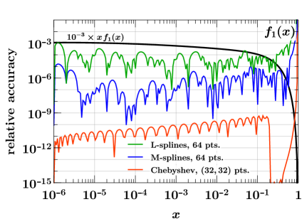
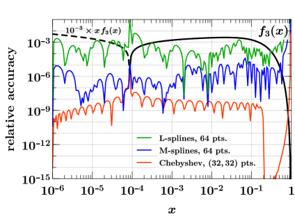
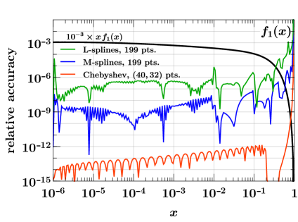
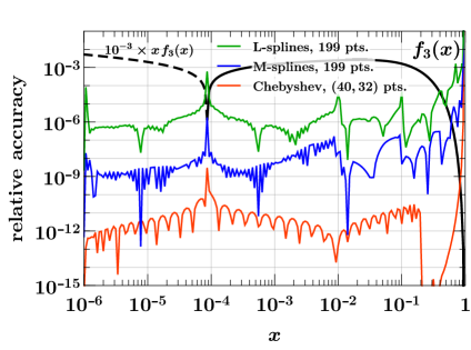
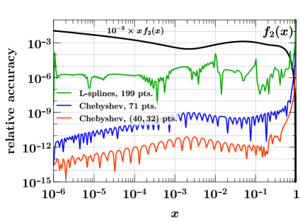
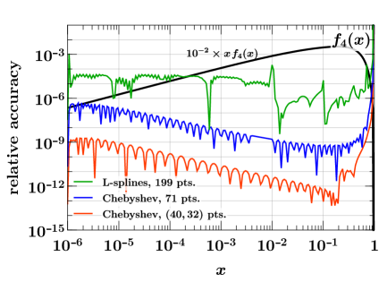
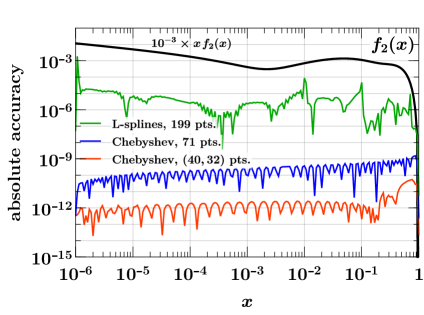
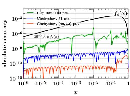
In figure -118 we compare the spline interpolation on the low-density grid (MMHT2014 grid with $n_{\mathrm{pts}}=64$) with Chebyshev interpolation on a $(32,32)$-point grid, which has nearly the same total number of points ($n_{\mathrm{pts}}=63$). The M-splines turn out to be more accurate than the L-splines, but this comes at the expense of them being more complex to construct. The Chebyshev interpolation achieves a significantly higher accuracy by several orders of magnitude than either of the splines. This reflects that, contrary to splines, Chebyshev interpolation uses polynomials of a high degree. In figure -118, we compare splines on the high-density grid (HERAPDF2.0 grid with $n_{\mathrm{pts}}=199$) with Chebyshev interpolation on a $(40,32)$-point grid with a total of $n_{\mathrm{pts}}=71$. Here, even with less than half the number of points, the Chebyshev interpolation achieves several orders of magnitude higher accuracy. This also highlights that the interpolation accuracy scales much better with the number of points for Chebyshev interpolation than for splines.

In figure -116 we compare the accuracy of interpolation on a single Chebyshev grid with the accuracy obtained with the two subgrids used in figure -118. We see that for the same total number of points, interpolation on two subgrids is more accurate, as anticipated above.

We observe in figures -118 to -116 that the relative accuracy varies with $x$ for Chebyshev interpolation somewhat more than it does for splines. In fact, the absolute accuracy of Chebyshev interpolation varies much less with $x$, as can be seen by comparing figure -116 with figure -116. The opposite holds for splines, where the relative accuracy shows less variation than the absolute one. This reflects that Chebyshev interpolation is “global” over the full interpolation interval, whilst splines are quite “local” (although the continuity conditions for neighboring splines lead to some correlation over larger distances in $x$).

As is seen in figures -118 to -116, the relative accuracy degrades in the limit $x\to 1$ for both splines and Chebyshev interpolation. This is not surprising, because in this limit the PDFs in eq. (3.1) approach zero. Moreover, they behave like $(1-x)^{\beta}$ with noninteger $\beta$ and are hence nonanalytic at $x=1$. This behavior cannot be accurately reproduced by interpolating polynomials in the vicinity of $x=1$, whatever their degree. We emphasize that this problem concerns the relative interpolation accuracy. As seen in figure -116, the absolute error of interpolation does remain small for $x$ up to $1$, as is expected from eq. (2.12). This is sufficient for many practical purposes, including the evaluation of convolution integrals that appear in cross sections or evolution equations. If high relative accuracy is required at large $x$, one needs to use subgrids with a sufficient number of points tailored to the region of interest.

3.3 Differentiation and integration

We now turn to Chebyshev interpolation for derivatives of the function $\tilde{f}(x)=xf(x)$. We use the barycentric formula (2.17) and its analog for the second derivative, multiplying of course with the Jacobian for the variable transformation from $t$ to $x$. For comparison, we also take the numerical derivative $(\tilde{f}_{\text{sp}}(x+h)-\tilde{f}_{\text{sp}}(x-h))/2h$ of the L-spline interpolant $\tilde{f}_{\text{sp}}(x)$. We use a variable step size $h=10^{-4}\,x$, having verified that the result remains stable when decreasing $h$ even further. The second derivative of $\tilde{f}_{\text{sp}}$ is evaluated in an analogous way.

Figure -115: Relative accuracy of the first derivative (top) and second derivative (bottom) for Chebyshev interpolation (red) and numerical differentiation of L-splines (green). The grids used on the left have lower $n_{\mathrm{pts}}$ as in figure -118, and those on the right have higher $n_{\mathrm{pts}}$ as in figure -118.

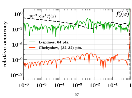
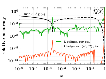
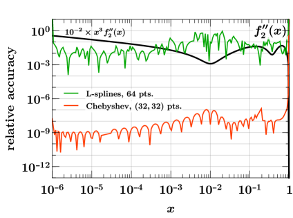
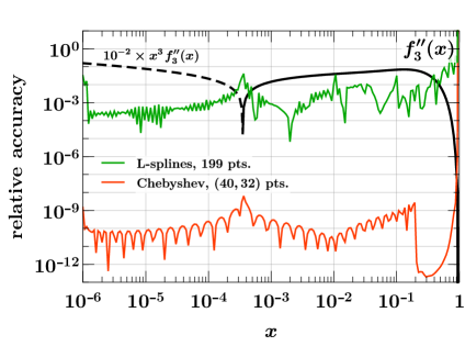
In figure -115 we consider the quantities

$$x^{2}f^{\mskip 1.5mu\prime}(x) =x\mskip 1.5mu\tilde{f}^{\mskip 1.5mu\prime}(x)-\tilde{f}(x)\,, x^{3}f^{\mskip 1.5mu\prime\prime}(x) =x^{2}\mskip 1.5mu\tilde{f}^{\mskip 1.5mu\prime\prime}(x)-2x\mskip 1.5mu\tilde{f}^{\mskip 1.5mu\prime}(x)+2\tilde{f}(x)$$ (3.6)

and the accuracy of evaluating them using the two methods just described. We see that with Chebyshev interpolants, a significantly higher accuracy is obtained. This is not surprising, since the polynomials approximating the derivatives are of a high degree in that case, whereas with cubic splines, one locally has a quadratic polynomial for the first derivative and a linear approximation for the second derivative. For the low-density grid with $n_{\mathrm{pts}}=64$, the L-splines in fact give errors around $10\%$ for the first and $100\%$ for the second derivative in parts of the $x$ range. We note that on each Chebyshev grid, the absolute accuracy of the derivatives (not shown here) has a milder variation in $x$ than the relative one, following the pattern we saw in figure -116 for $xf(x)$ itself.

Figure -114: Relative accuracy of the truncated Mellin moments (3.7) with $x_{0}=10^{-9}$ and with $j=2$ (top) or $j=10$ (bottom), for $f_{2}(x)$ (left) or $f_{4}(x)$ (right). We use Chebyshev grids with $k=1$ to $4$ subgrids and $n_{\mathrm{pts}}/k$ points per subgrid, namely $[x_{0},1]$ (blue), $[x_{0},0.2,1]$ (red), $[x_{0},10^{-3},0.5,1]$ (green), and $[x_{0},10^{-6},10^{-3},0.5,1]$ (yellow). The results for different $n_{\mathrm{pts}}$ are connected by lines to guide the eye.

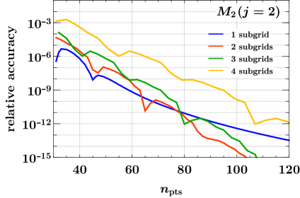
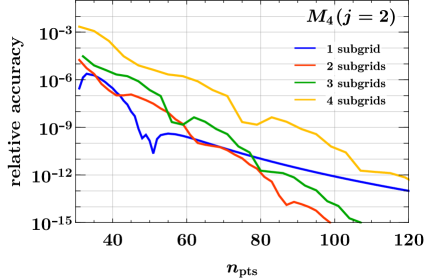
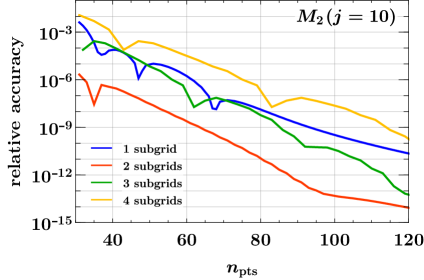
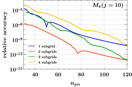
To explore the accuracy of numerical integration, we consider the truncated Mellin moments

$$M_{i}(j) =\int_{x_{0}}^{1}\mathrm{d}x\;x^{j-1}\,f_{i}(x)\,,$$ (3.7)

where the lower integration limit is the lowest point $x_{0}$ of the grid. In figure -114, we show the dependence of the relative accuracy on the total number of grid points when using $1$ to $4$ subgrids of equal size. The advantage of using subgrids is clearly seen, especially for high moment index $j$, which emphasizes the large $x$ region of the integrand. We find that taking 2 or 3 subgrids gives best results for a wide range of $j$. The disadvantage of using interpolants with lower polynomial degree becomes the dominant limiting factor with 4 or more subgrids.

3.4 Estimating the numerical accuracy

Let us now take a closer look at methods to estimate the numerical accuracy of interpolation or integration with Chebyshev polynomials. An obvious option is to re-compute the quantity of interest with an increased number of points. However, the examples in figure -114 show that the accuracy is not a strictly decreasing function of $n_{\mathrm{pts}}$, and we see fluctuations with local minima and maxima as $n_{\mathrm{pts}}$ varies by about $10$ units. For a reliable estimate, one should therefore take a sufficiently large increase in $n_{\mathrm{pts}}$. Increasing $n_{\mathrm{pts}}$ in several steps provides an additional way of ensuring that the estimate is trustworthy.

The procedure just described can give sound accuracy estimates and is what we will adopt for assessing the accuracy of DGLAP evolution in section 5.3. However, since the result must be evaluated multiple times on increasingly dense grids, this procedure can be computationally expensive, especially when the cost scales more than linearly with the number of grid points. This is indeed the case of DGLAP evolution, where the evaluation of convolution integrals involves $n_{\mathrm{pts}}\times n_{\mathrm{pts}}$ matrices.

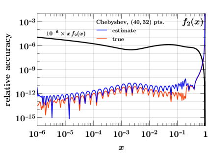
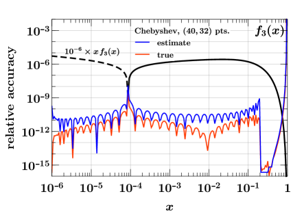
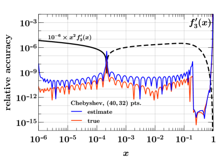
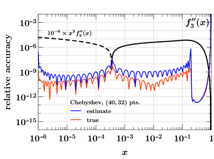
An alternative with much less computational overhead is to estimate the accuracy from the difference between Chebyshev interpolation and interpolation on the same grid without the end points, as described in section 2. This does not require any additional function evaluations. We compare this estimate with the actual interpolation accuracy in figure -113. In the subinterval for large $x$, the estimate is very close to the true error, whilst in the subinterval for small to intermediate $x$ it somewhat overestimates the actual numerical error. The amount of overestimation is highest close to the interval limits, which is not surprising, because this is where the two interpolation methods differ most. The corresponding comparison for differentiation is shown in figure -112 and follows the same pattern. We also note that the quality of the estimate for other sample PDFs is as good as or even better than in the examples shown here.

Figure -113: Comparison of the true relative interpolation accuracy (red) and its estimate (blue) obtained from the difference between interpolation on the Chebyshev grid with and without its end points. The $(40,32)$-point grid used is the same as in figure -118.

Figure -112: Comparison of true (red) and estimated (blue) interpolation accuracy as in figure -113, but for the first and second derivative of the sample PDF $f_{3}(x)$.

Figure -111: Comparison of the relative integration accuracy (solid) and its estimate (dashed) for Clenshaw-Curtis (red) and Gauss-Kronrod (green) quadrature. The considered integrals are the truncated Mellin moments $M_{i}(j)$ of the test functions $f_{i}(x)$ with $i=2,3$. For both methods we use two subgrids $[10^{-9},0.2,1]_{(41,\mskip 1.5mu31)}$ with the appropriate Chebyshev or Gauss-Kronrod points for the integration variable $\ln x$. In the accuracy estimates, the results for a given integration rule are first added for the two subintervals, and then the absolute difference between the involved higher-order and lower-order rules is taken.

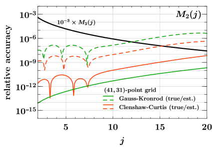
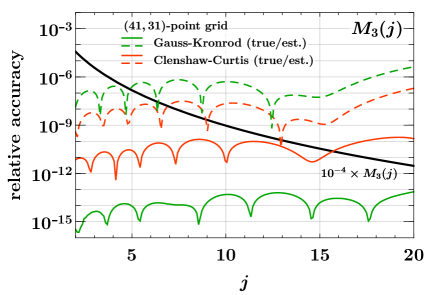
The analog for integration of the previous method is to estimate the accuracy of Clenshaw-Curtis integration from the difference to the Fejér quadrature rule. In figure -111, we compare this estimate with the actual numerical error for the Mellin moment (3.7). We find that it tends to overestimate the actual error by two to three orders of magnitude, which is more than what we saw for interpolation. For comparison, we also show the relative accuracy obtained with the widely used Gauss-Kronrod rule, using the same two subintervals and the same number of grid points per subinterval as for Clenshaw-Curtis. As is commonly done, the accuracy estimate for Gauss-Kronrod is obtained from the difference between the nominal Gauss-Kronrod rule and the lower-order Gauss rule on a subset of the grid points. We see that the Gauss-Kronrod rule has the highest accuracy. In practical applications, the true result is however not known, and an integrator is only as good as its accuracy estimation. Here, the accuracy estimate for Gauss-Kronrod is much worse than our estimate for Clenshaw-Curtis. As discussed at the end of section 2, this is not unexpected given the comparison of polynomials orders, but it is interesting to see that the quantitative effect can be as pronounced as in our examples. We also note that the quantitative differences between the integration methods vary significantly with the shape of the integrands, as is evident from the two panels in figure -111.

Overall, as far as numerical accuracy estimates are concerned, using interpolation, differentiation, or integration without the end points of a Chebyshev grid can be considered as an inexpensive estimate of reasonable quality. It is not an alternative to the high-quality estimate one can achieve by a stepwise increase in the number of grid points. Its biggest advantage is thus to provide a fast and reliable indicator whether the accuracy of a result is sufficient or calls for a dedicated, more expensive investigation.

4 Mellin convolution

In this section, we consider the Mellin convolution of a PDF with an integral kernel, such as a DGLAP splitting function, a beam-function matching kernel, or a hard-scattering coefficient. In terms of the scaled PDF $\tilde{f}(x)=xf(x)$, we wish to compute

$$\bigl{(}K\otimes\tilde{f}\,\bigr{)}(x) =\int_{x}^{1}\frac{\mathrm{d}z}{z}\,K(z)\,\tilde{f}\left(\frac{x}{z}\right)\,.$$ (4.1)

Here, $K(z)$ is the scaled kernel, given e.g. by $K(z)=z\mskip 1.5muP(z)$ for a DGLAP splitting function $P(z)$.

Let us see how eq. (4.1) can be evaluated in a discretized setting. For simplicity, we first consider a single Chebyshev grid for the range $x_{0}\leq x\leq 1$ as described in section 3.1. The convolution $(K\otimes\tilde{f})(x)$ is a function of $x$ over the same domain as $\tilde{f}(x)$. Hence, we can interpolate it in complete analogy to $\tilde{f}(x)$ itself. For this purpose, we only need to evaluate eq. (4.1) at the grid points $x_{i}$,

$$\bigl{(}K\otimes\tilde{f}\,\bigr{)}(x_{i}) =\int_{x_{i}}^{1}\!\frac{\mathrm{d}{z}}{z}\,K(z)\,\tilde{f}\left(\frac{x_{i}}{z}\right)\approx\int_{x_{i}}^{1}\frac{\mathrm{d}{z}}{z}\,K(z)\,\sum_{j=0}^{N}\tilde{f}_{j}\,b_{j}\left(\ln\frac{x_{i}}{z}\right)\,,$$ (4.2)

where in the last step we used the barycentric formula (3.2) to interpolate $\tilde{f}(x_{i}/z)$ under the integral. Introducing the kernel matrix

$$K_{ij} =\int_{x_{i}}^{1}\frac{\mathrm{d}{z}}{z}\,K(z)\,b_{j}\left(\ln\frac{x_{i}}{z}\right)\,,$$ (4.3)

we can compute the function values of $K\otimes\tilde{f}$ on the grid by a simple matrix multiplication,

$$\bigl{(}K\otimes\tilde{f}\,\bigr{)}(x_{i}) \approx\sum_{j=0}^{N}K_{ij}\mskip 1.5mu\tilde{f}_{j}\,.$$ (4.4)

Importantly, the matrix $K_{ij}$ only depends on the given kernel and grid but not on $\tilde{f}$. It can thus be pre-computed once using standard numerical integration routines.

In general, $K(z)$ is a distribution rather than an ordinary function. Restricting ourselves to plus and delta distributions, we write

$$K(z) =K_{\text{sing}}(z)+K_{\text{reg}}(z)+\delta(1-z)\,K_{\delta}\,,$$ (4.5)

where $K_{\text{sing}}(z)$ is the singular part of the kernel and contains plus distributions. The function $K_{\text{reg}}(z)$ contains at most an integrable singularity at $z=1$, for instance powers of $\ln(1-z)$. The separation between $K_{\text{sing}}$ and $K_{\text{reg}}$ is not unique and may be adjusted as is convenient. The convolution (4.1) can now be written as

$$\bigl{(}K\otimes\tilde{f}\,\bigr{)}(x) =\int_{x}^{1}\frac{\mathrm{d}{z}}{z}\,K_{\text{sing}}(z)\left[\tilde{f}\left(\frac{x}{z}\right)-\tilde{f}(x)\right]+\int_{x}^{1}\!\frac{\mathrm{d}{z}}{z}\,K_{\text{reg}}(z)\,\tilde{f}\left(\frac{x}{z}\right)+K_{d}(x)\,\tilde{f}(x)\,,$$ (4.6)

where

$$K_{d}(x) =K_{\delta}+\int_{x}^{1}\frac{\mathrm{d}{z}}{z}\,K_{\text{sing}}(z)$$ (4.7)

can be evaluated analytically if the separation between $K_{\text{sing}}$ and $K_{\text{reg}}$ is chosen appropriately. Due to the explicit subtraction of $\tilde{f}(x)$ in the first integral in eq. (4.6), the plus prescription in $K_{\text{sing}}$ can now be omitted, because

$$\int_{x}^{1}\!\mathrm{d}{z}\,\bigl{[}g(z)\bigr{]}_{+}\;h(z) =\int_{x}^{1}\!\mathrm{d}{z}\,g(z)\,h(z)\qquad\text{for}\quad h(1)=0\,.$$ (4.8)

From the definition (4.7) one readily finds that $K_{d}(x)$ diverges like $\ln^{n+1}(1-x)$ for $x\to 1$ if $K(z)$ contains a term $\mathcal{L}_{n}(1-z)$, where we write

$$\mathcal{L}_{n}(y)=\biggl{[}\frac{\ln^{n}(y)}{y}\biggr{]}_{+}$$ (4.9)

for the logarithmic plus distribution of degree $n$. However, a PDF vanishes much faster for $x\to 1$ than $K_{d}(x)$ diverges, such that the product $K_{d}(x)\,\tilde{f}(x)$ tends to zero in that limit.

Applying eq. (4.6) to the evaluation of the $K_{ij}$ matrix in eq. (4.3), we have

$$K_{ij} =\int_{u_{i}}^{0}\!\mathrm{d}v\;K_{\text{sing}}(e^{v})\,\bigl{[}b_{j}(u_{i}-v)-\delta_{ij}\bigr{]}+\int_{u_{i}}^{0}\!\mathrm{d}v\;K_{\text{reg}}(e^{v})\,b_{j}(u_{i}-v)+\delta_{ij}\,K_{d}(x_{i})\,,$$ (4.10)

where $u_{i}$ and $u_{j}$ are grid points in $u$, and where we have changed the integration variable to $v=\ln z$. The plus prescription in $K_{\text{sing}}$ can again be omitted, because the term in square brackets vanishes at least linearly in $v$ for $v\to 0$. Hence, all integrals can be evaluated numerically, for which we use an adaptive Gauss-Kronrod routine.

Given that $x_{N}=1$, the matrix element $K_{N\mskip-1.5muN}$ is ill defined if $K$ contains a plus distribution, because $K_{d}(x)$ diverges for $x\to 1$ in that case. This does not present any problem: we already noticed that $K_{d}(x)\,\tilde{f}(x)\to 0$ for $x\to 1$, which translates to $K_{N\mskip-1.5muN}\mskip 1.5mu\tilde{f}_{N}=0$ in the discretized version. This term may hence be omitted in the matrix multiplication (4.4), along with all other terms $K_{iN}\mskip 1.5mu\tilde{f}_{N}$.

It is not difficult to generalize the preceding discussion to the case of several subgrids in $u$, each of which is mapped onto a Chebyshev grid. One then has a distinct set of barycentric basis functions for each subgrid. If $u_{j}$ and $u_{i}-v$ are not on the same subgrid, then the basis function $b_{j}(u_{i}-v)$ in eq. (4.10) must be set to zero. As a consequence, the matrix $K_{ij}$ has blocks in which all elements are zero. Let us, however, note that $K_{ij}$ always has nonzero elements below the diagonal $i=j$ and is not an upper triangular matrix.

We now study the numerical accuracy of this method relative to the exact result, which we obtain by the direct numerical evaluation of the convolution integral (4.6). For comparison, we also show the accuracy of the result obtained by approximating $\tilde{f}(x)$ in eq. (4.6) with its L-splines interpolant and performing the convolution integral numerically. All explicit numerical integrals in this study are performed at sufficiently high precision to not influence the results.

Figure -110: Relative accuracy of Mellin convolutions. The red curves correspond to Chebyshev interpolation for both the PDF and the convolution result, as described in the text. The green curves are obtained by performing the numerical convolution integral for the PDF interpolated with L-splines. Details about the convolution kernels are given in the text. On the left, we use the same grids as in figure -118, with $n_{\mathrm{pts}}=63$ for Chebyshev interpolation and $n_{\mathrm{pts}}=64$ for L-splines. On the right, we use the Chebyshev grid $[10^{-9},0.2,1]_{(40,32)}$ with $n_{\mathrm{pts}}=71$ and for L-splines a grid with $n_{\mathrm{pts}}=150$ (corresponding to the NNPDF3.1 grid in table 1).

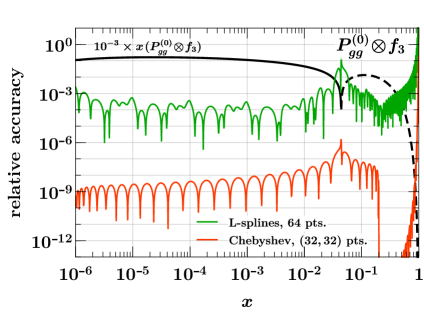
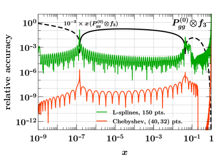
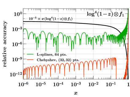
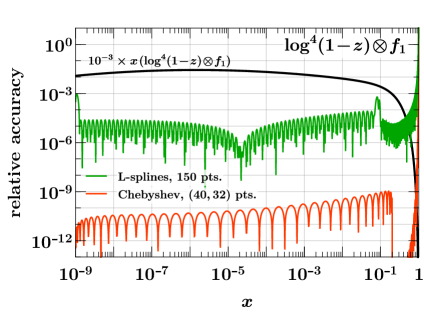
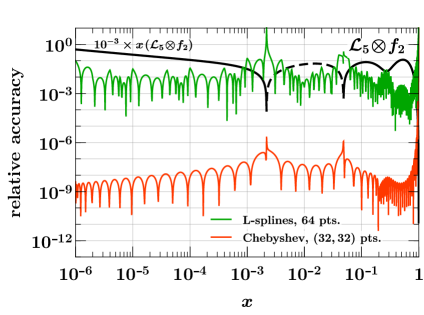
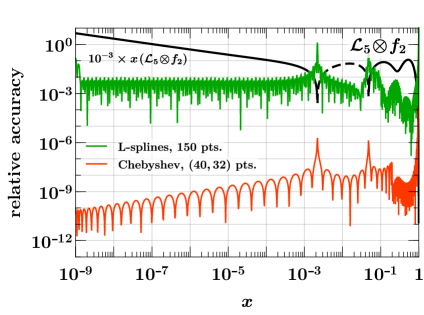
In figure -110, we show the results of this exercise for the convolution of our sample PDFs $f_{i}(x)$ with kernels that have different singular behavior at the end point $z=1$. The kernel in the top row is the leading-order DGLAP splitting function $P_{gg}$, which contains a term $\mathcal{L}_{0}(1-z)$. The kernel in the second row is $\ln^{4}(1-z)$, which is the most singular term in the three-loop splitting functions $P_{gq}$ and $P_{qg}$ [63, 64]. In the bottom row, we take $\mathcal{L}_{5}(1-z)$ as kernel, which appears in the N³LO corrections to the rapidity spectrum of inclusive Higgs production in $pp$ collisions [15]. In all cases, the accuracy of our Chebyshev based method is several orders of magnitude higher than the one obtained when interpolating PDFs with L-splines and then performing the convolution integral.

The numerical inaccuracies for the convolution with $\mathcal{L}_{5}(1-z)$ using L-splines are in the percent range over a wide range of $x$ and much higher than those for the other kernels we looked at. This is in line with the results of ref. [15], which finds that the convolution of $\mathcal{L}_{5}(1-z)$ with PDFs from the LHAPDF library can lead to considerable numerical instabilities. The PDFs used in that work are those of the NNPDF3.0 analysis [65], and for the sake of comparison we use the corresponding grid for spline interpolation in the plots on the right of figure -110.

An alternative method to evaluate the convolution is to use the Chebyshev interpolant of $\tilde{f}$ and perform the convolution integral itself numerically, analogous to what we did with L-splines above. This avoids the additional interpolation of $(K\otimes\tilde{f})$ that happens in the above kernel matrix method. The numerical accuracy of this alternative method differs slightly from the accuracy of the kernel matrix method, but it is of the same order of magnitude. Hence, the additional interpolation of $(K\otimes\tilde{f})$ does not introduce a significant penalty in accuracy beyond that of interpolating $\tilde{f}$ itself. This makes the kernel matrix method far more attractive, as it avoids the evaluation of a numerical integral for each desired $\tilde{f}$ and $x$.

5 DGLAP evolution

5.1 Numerical solution of DGLAP equations

In this section, we present our approach to the numerical solution of the DGLAP evolution equations [66, 67, 68]. Up to order $\alpha_{s}^{n+1}$, they read

$$\frac{\mathrm{d}f(x,\mu)}{\mathrm{d}\ln\mu^{2}} =\sum_{m=0}^{n}\,\left[\frac{\alpha_{s}(\mu)}{4\pi}\right]^{m+1}\,\bigl{(}P^{(m)}\otimes f(\mu)\bigr{)}(x)\,,$$ (5.1)

where $P^{(m)}$ is the splitting function at order $m$. For notational simplicity, we suppress the indices for the parton type and the associated sum on the right-hand side. To solve eq. (5.1), we discretize the scaled PDFs $\tilde{f}(x)=xf(x)$ on a Chebyshev grid and evaluate the Mellin convolutions on the right-hand side as discussed in section 4. The integro-differential equation (5.1) then turns into a coupled system of ordinary differential equations (ODEs),

$$\frac{\mathrm{d}\tilde{f}_{i}(\mu)}{\mathrm{d}\ln\mu^{2}} =\sum_{j=0}^{N}\,\sum_{m=0}^{n}\,\left[\frac{\alpha_{s}(\mu)}{4\pi}\right]^{m+1}\,\widetilde{P}_{ij}^{(m)}\,\tilde{f}_{j}(\mu)\,,$$ (5.2)

where $\tilde{f}_{i}(\mu)=\tilde{f}(x_{i},\mu)$ and $\widetilde{P}_{ij}^{(m)}$ is the kernel matrix for $K(z)\equiv zP^{(m)}(z)$ as defined in eq. (4.3). This system of ODEs can be solved numerically using the standard Runge-Kutta algorithm, which is described in more detail in appendix A. This formulation as a linear system of ODEs by discretization in $x$ is common to many approaches that solve the DGLAP equations in $x$ space [17, 18, 19, 26, 25, 27]. By using the Chebyshev grid for the discretization in $x$, the resulting evolved PDF can then be Chebyshev interpolated.

The Runge-Kutta algorithm uses a discretization of the evolution variable $t$ (not to be confused with the argument of Chebyshev polynomials in section 2). It is advantageous if the function multiplying $\tilde{f}$ on the right-hand side of the evolution equation depends only weakly on $t$, because this tends to give a uniform numerical accuracy of evolution with a fixed step size in $t$. We therefore evolve in the variable

$$t =-\ln\alpha_{s}(\mu)$$ (5.3)

instead of $\ln\mu^{2}$. For the running coupling at order $n$, we write

$$\frac{\mathrm{d}\mskip 1.5mu\alpha_{s}^{-1}}{\mathrm{d}\ln\mu^{2}} =-\frac{\beta(\alpha_{s})}{\alpha_{s}^{2}}=\sum_{m=0}^{n}\frac{\beta_{m}}{4\pi}\,\left(\frac{\alpha_{s}}{4\pi}\right)^{m}$$ (5.4)

and use a Runge-Kutta routine (see the end of appendix A) to solve for $\alpha_{s}^{-1}$ as a function of $\ln\mu^{2}$. At leading order, the DGLAP equation (5.1) then becomes

$$\frac{\mathrm{d}f(t)}{\mathrm{d}t}=\frac{1}{\beta_{0}}\,P^{(0)}\otimes f(t)\,.$$ (5.5)

with no explicit $t$ dependence on the right-hand side. Using $\alpha_{s}=e^{-t}$, we have at NLO

$$\frac{\mathrm{d}f(t)}{\mathrm{d}t}=\frac{1}{\beta_{0}+(\beta_{1}/4\pi)\,e^{-t}}\biggl{[}P^{(0)}+\frac{P^{(1)}}{4\pi}\,e^{-t}\biggr{]}\otimes f(t)\,,$$ (5.6)

where an explicit $t$ dependence appears in the two-loop terms with $\beta_{1}$ and $P^{(1)}$. The corresponding equations at NNLO and higher are easily written down.

The pattern of mixing between quarks, antiquarks, and gluons under DGLAP evolution is well known. Its structure at NNLO is given in refs. [69, 63] and remains the same at higher orders. To reduce mixing to a minimum, we work in the basis formed by

$$g, \Sigma^{\pm}=\sum_{i}q_{i}^{\pm},$$

$$u^{\pm}-d^{\pm}, d^{\pm}-s^{\pm}, s^{\pm}-c^{\pm}, c^{\pm}-b^{\pm}, b^{\pm}-t^{\pm}\,,$$ (5.7)

where $q^{\pm}=q\pm\bar{q}$. Contrary to the often-used flavor nonsinglet combinations $u+d-2s$, $u+d+s-3c$, etc., the differences between consecutive flavors in eq. (5.1) are less prone to a loss of numerical accuracy due to rounding effects in regions where the strange and heavy-quark distributions are much smaller than their counterparts for $u$ and $d$ quarks. Note that at NNLO, the combination $\Sigma^{-}$ has a different evolution kernel than the flavor differences in the second line of eq. (5.1). This is due to graphs that have a $t$ channel cut involving only gluons.

We implement the unpolarized splitting functions at LO and NLO in their exact analytic forms. For the unpolarized NNLO splitting functions, we use the approximate expressions given in refs. [69, 63], which are constructed from a functional basis containing only the distributions $\mathcal{L}_{0}(1-z)$, $\delta(1-z)$ and polynomials in $z$, $1/z$, $\ln z$, and $\ln(1-z)$. With these parameterizations, the numerical evaluation of the kernel matrices in all channels takes about as long for $P^{(2)}$ as it does for $P^{(1)}$.

Both $\alpha_{s}$ and the PDFs depend on the number $n_{F}$ of quark flavors that are treated as light and included in the $\overline{\text{MS}}$ renormalization of these quantities. For the conversion between $\alpha_{s}$ for different $n_{F}$, we use the matching conditions in ref. [70] at the appropriate order. For the transition between PDFs with different $n_{F}$, we implement the matching kernels given in ref. [71], which go up to order $\alpha_{s}^{2}$. We have verified that they agree with the independent calculation in ref. [72]. The Mellin convolutions of matching kernels with PDFs are also evaluated as described in section 4.

5.2 Validation

To validate our DGLAP evolution algorithm, we compare our results with the benchmark tables in section 1.33 of ref. [73] and section 4.4 of ref. [74]. These tables contain PDFs evolved to the scale $\mu=100\,\mathrm{GeV}$ from initial conditions given in analytic form at $\mu_{0}=\sqrt{2}\mskip 1.5mu\,\mathrm{GeV}$. Evolution is performed at LO, NLO and NNLO, either at fixed $n_{F}=4$ or with a variable number of flavors $n_{F}=3\dots 5$ and flavor transitions at scales $\mu_{c}$ and $\mu_{b}$. The default choice is $\mu_{c}=m_{c}=\sqrt{2}\,\mathrm{GeV}$ and $\mu_{b}=m_{b}=4.5\,\mathrm{GeV}$. We compare with the LO and NLO results in ref. [73] and with the NNLO results in ref. [74]. The latter are obtained with the same parameterized NNLO splitting functions that we use. Furthermore, the parameterization in eq. (3.5) of ref. [22] is used for the two-loop matching kernel for the transition from a gluon to a heavy quark. We also use this parameterization for the sake of the present comparison, noting that visible differences with the benchmark results appear when we use the exact analytic form for this kernel instead.

The benchmark tables were obtained using two programs, HOPPET [25] and QCD-Pegasus [22], both run with high-precision settings. The former solves the evolution equations in $x$ space, whilst the latter uses the Mellin moment technique. The tables give results for the evolved PDFs at 11 values of $x$ between $10^{-7}$ and $0.9$. The results are given with five significant digits, with the exception of several sea-quark combinations at $x=0.9$, which are very small and are given to only four significant digits.

As specified in ref. [73], evolution with HOPPET was performed by using seventh-order polynomials for the interpolation on multiple $x$ grids spanning the interval $[10^{-8},1]$ with a total of $n_{\mathrm{pts}}=1,\!170$. A uniform grid in $\ln\mu^{2}$ was used, with 220 points between $\mu=\sqrt{2}\mskip 1.5mu\,\mathrm{GeV}$ and $1000\,\mathrm{GeV}$. The results were verified to be stable within a $10^{-5}$ relative error for $x<0.9$ by comparing them with the results of the same program with half the number of points on both the $x$ and the $\mu$ grids. Furthermore, they were compared with the results obtained with QCD-Pegasus.

For the comparison with our approach, we use a Chebyshev grid with 3 subgrids $[10^{-8},10^{-3},0.5,1]_{(24,\mskip 1.5mu24,\mskip 1.5mu24)}$ which has $n_{\mathrm{pts}}=70$. The DGLAP equations are solved using a Runge-Kutta algorithm with the DOPRI8 method (see appendix A) and a maximum step size in $t$ of $h=0.1$. This amounts to about 12 Runge-Kutta steps from the starting scale to $\mu=100\,\mathrm{GeV}$. Our results for the benchmark numbers (rounded as stated above) remain the same if we take $40$ instead of $24$ points for each subgrid in $x$. They also remain unchanged if we use the same Runge-Kutta method with maximum step size $h=0.3$ or $h=0.02$.

We compare our results with the numbers reported in tables 2, 3, 4 of ref. [73] and in tables 14 and 15 of ref. [74], which cover unpolarized evolution both with fixed $n_{F}=4$ and with variable $n_{F}=3\ldots 5$. Whilst the tables also give results for evolution with different scales $\mu_{\text{r}}$ in $\alpha_{s}$ and $\mu_{\text{f}}$ in the PDFs, we always set $\mu_{\text{r}}=\mu_{\text{f}}$. We agree with all benchmark numbers, except for those given in our tables 3 and 3. In all cases where we differ, the differences can be attributed to the benchmark results and fall into two categories:

1. The benchmark tables contain a number of entries, marked by an asterisk, for which the results of the two used codes differ in the sixth digit and give different numbers when rounded to five digits. The number with the smaller modulus is then given in the tables. In several cases, our result agrees with number with the larger modulus and in this sense agree with the benchmark results.

2. We differ from the benchmark numbers in five more cases. For the two cases at NNLO, the benchmark results have typographical errors in the exponent. In the other three cases, we differ by one unit in the fifth digit. We contacted the authors of the benchmark tables, who confirmed that indeed their respective codes agree with our numbers [75].

order	$x$	$xu_{v}$	$xd_{v}$	$xL_{-}$	$2xL_{+}$	$xs_{+}$	$xc_{+}$	$g$
LO	$0.5$					$7.3137^{-4}$
	$0.9$						$4.8894^{-9}_{*}$
NLO	$10^{-7}$					$6.6914^{+1}_{*}$		$1.1484^{+3}_{*}$
	$10^{-4}$							$9.2873^{+1}_{*}$
	$10^{-3}$				$6.1649^{+0}_{*}$
	$10^{-2}$					$8.4221^{-1}_{*}$

Table 2: Results for evolution with $n_{F}=4$ for which we differ from the numbers in the benchmark tables in ref. [73]. The notation for PDF combinations is $L_{\pm}=\bar{d}\pm\bar{u}$ and $q_{+}=q+\bar{q}$ for $q=s,c$. The number format $a^{b}$ is shorthand for $a\times 10^{b}$. As discussed in the text, all differences can be attributed to the benchmark results, where entries with an asterisk correspond to category 1 and the entry in blue corresponds to category 2. We note that in the table headers of ref. [73] it should read $2xL_{+}$ instead of $xL_{+}$.

order	$x$	$xu_{v}$	$xd_{v}$	$xL_{-}$	$2xL_{+}$	$xs_{+}$	$xc_{+}$	$xb_{+}$	$g$
LO	$10^{-7}$							$4.6071^{+1}$
NLO	$10^{-6}$								$5.2290^{+2}_{*}$
	$0.7$	$2.0102^{-2}$
NNLO	$10^{-7}$		$1.0699^{-4}$						$9.9694^{+2}$

Table 3: As table 3, but for evolution and flavor matching from $n_{F}=3\ldots 5$. The corresponding benchmark tables are in ref. [73] for LO and NLO and in ref. [74] for NNLO.

5.3 Numerical accuracy

We now study the numerical accuracy of our method in some detail. We use $x_{0}=10^{-7}$ and 3 subgrids. The evolution equations are solved with the DOPRI8 method (see appendix A). To assess the accuracy, we compare three settings with different numbers of grid points and different Runge-Kutta steps $h$:

1. $[10^{-7},10^{-2},0.5,1]_{(24,\mskip 1.5mu24,\mskip 1.5mu24)}$ ($n_{\mathrm{pts}}=70$) and $h=0.1$,

2. $[10^{-7},10^{-2},0.5,1]_{(40,\mskip 1.5mu40,\mskip 1.5mu40)}$ ($n_{\mathrm{pts}}=118$) and $h=0.1$,

3. $[10^{-7},10^{-2},0.5,1]_{(40,\mskip 1.5mu40,\mskip 1.5mu40)}$ ($n_{\mathrm{pts}}=118$) and $h=0.004$.

To estimate the numerical error due to the discretization in $x$, we take the difference between settings 1 and 2, whereas the error due to the Runge-Kutta algorithm is estimated from the difference between settings 2 and 3. For the combined error, we take the difference between settings 1 and 3. Note that these estimates correspond to the accuracy of setting 1. We use the same initial conditions at $\mu_{0}=\sqrt{2}\mskip 1.5mu\,\mathrm{GeV}$ as in the benchmark comparison described in the previous subsection. Starting at $n_{F}=3$, heavy flavors are added at $m_{c}=\sqrt{2}\mskip 1.5mu\,\mathrm{GeV}$, $m_{b}=4.5\,\mathrm{GeV}$, and $m_{t}=175\,\mathrm{GeV}$. In the remainder of this section, we always evolve and match at NNLO.

Figure -109: Relative numerical accuracy of NNLO DGLAP evolution and flavor matching from $\mu_{0}=\sqrt{2}\mskip 1.5mu\,\mathrm{GeV}$ and $n_{F}=3$ to $\mu=100\,\mathrm{GeV}$ and $n_{F}=5$. We use the PDFs defined in refs. [73, 74]. The top row shows quark, antiquark, and gluon distributions (with $f_{\text{sea}}\in\{\bar{u},\bar{d},s,\bar{s},c,\bar{c},b,\bar{b}\}$), and the bottom row shows the differences $q-\bar{q}$.

Figure -108: As figure -109, but for evolution and flavor matching up to $\mu=10\,\mathrm{TeV}$ and $n_{F}=6$.

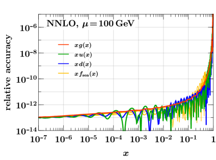
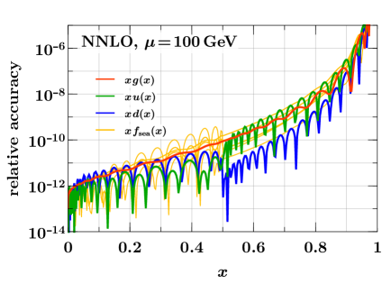
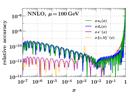
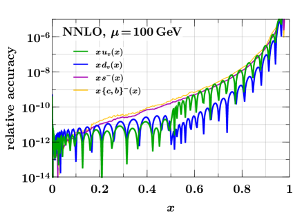
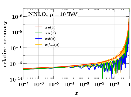
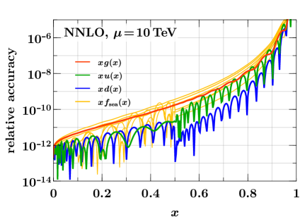
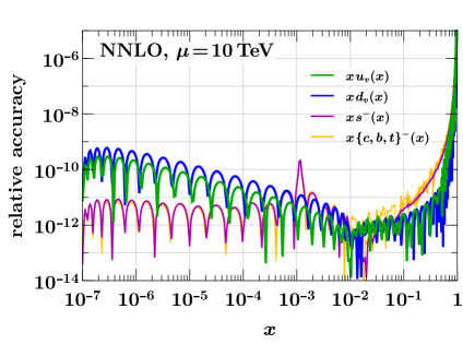
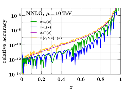
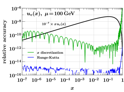
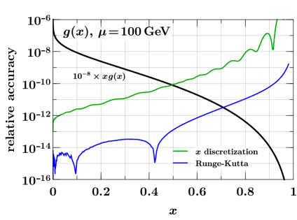
The combined discretization and Runge-Kutta accuracy for evolution to $\mu=100\,\mathrm{GeV}$ and $\mu=10\,\mathrm{TeV}$ is shown in figures -109 and -108, respectively, both for the individual parton flavors $g$, $q$, $\bar{q}$, and for the valence combinations $q^{-}=q-\bar{q}$. The relative accuracy is better than $10^{-7}$ up to $x\leq 0.8$, and much better than that for smaller $x$. The same holds when we evolve to $\mu=1.01\mskip 1.5mum_{c}$ or $\mu=1.01\mskip 1.5mum_{b}$, where the charm or bottom distributions are very small. The relative accuracy of $u_{v}$ and $d_{v}$ increases towards small $x$. This reflects the strong decrease of these distributions in the small-$x$ limit, as we already observed and explained in section 3. The combinations $s^{-}$, $c^{-}$, $b^{-}$, and $t^{-}$ show less variation at small $x$, and so does their relative accuracy.

In figure -107 we show examples for the separate errors due to discretization and the Runge-Kutta algorithm. With our settings, the overall numerical accuracy is entirely determined by the discretization in $x$, whilst the inaccuracy due to the Runge-Kutta algorithm can be neglected. The Runge-Kutta accuracy for $u_{v}$ is in fact determined by the machine precision except for very large $x$, as signaled by the noisy behavior of the error curve.

Figure -107: Relative accuracy of NNLO DGLAP evolution and flavor matching, distinguishing the contributions due to $x$-space discretization (green) and the Runge-Kutta algorithm (blue). The plot on the left shows $x\mskip 1.5muu_{v}(x)$ and the plot on the right $x\mskip 1.5mug(x)$. Notice the different scales in $x$.

It is often found that backward evolution, i.e. evolution from a higher to a lower scale, is numerically unstable. The structure of the DGLAP equations is such that the relative uncertainties (physical or numerical) of PDFs become larger when one evolves from a scale $\mu_{1}$ to a lower scale $\mu_{0}$. This property is shared by other renormalization group equations in QCD, including the one for $\alpha_{s}(\mu)$. To which extent it leads to numerically unreliable results is, however, a separate question.

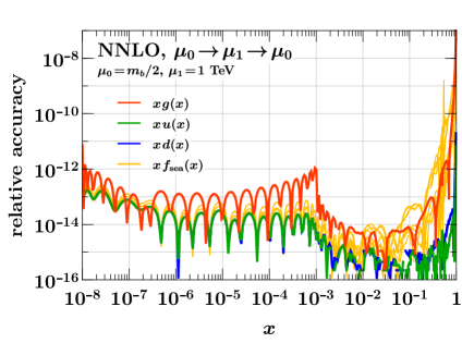
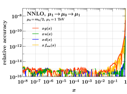
To study backward evolution within our method, we perform the following exercise. We start with the input PDFs of the benchmark comparison, evolve them with $n_{F}=4$ from $\sqrt{2}\mskip 1.5mu\,\mathrm{GeV}$ to $m_{b}/2=2.25\,\mathrm{GeV}$ and match to $n_{F}=5$ at that point. The result is taken as initial condition for $n_{F}=5$ evolution from $\mu_{0}=2.25\,\mathrm{GeV}$ to $\mu_{1}=1\,\mathrm{TeV}$ (step 1). The result of step 1 is evolved down to $\mu_{0}$ (step 2), and the result of step 2 is again evolved up to $\mu_{1}$ (step 3). We thus have two quantities that are sensitive to the accuracy of backward evolution:

• the difference between the output of step 2 and the input to step 1, which corresponds to the evolution path $\mu_{0}\to\mu_{1}\to\mu_{0}$,

• the difference between the output of step 3 and the input to step 2, corresponding to the evolution path $\mu_{1}\to\mu_{0}\to\mu_{1}$.

The relative accuracy for the two evolution paths is shown in figure -106 for the DOPRI8 method with maximum step size $h=0.1$. In both cases, we find very high accuracy, in some cases near machine precision as signaled by the noisy behavior of the curves. Relative errors tend to be larger for the evolution path $\mu_{0}\to\mu_{1}\to\mu_{0}$, but they are all below $10^{-8}$ for $x\leq 0.9$ (except in the vicinity of zero crossings). Note that a high accuracy is also obtained for the small combinations $s^{-}$, $c^{-}$, and $b^{-}$, which are induced by evolution at order $\alpha_{s}^{3}$.

Figure -106: Relative accuracy of NNLO DGLAP evolution at fixed $n_{F}=5$ from $\mu_{0}\to\mu_{1}\to\mu_{0}$ (left) and from $\mu_{1}\to\mu_{0}\to\mu_{1}$ (right). The scales are $\mu_{0}=2.25\,\mathrm{GeV}$ and $\mu_{1}=1\,\mathrm{TeV}$, and the DOPRI8 method with maximum step size $h=0.1$ is used to solve the evolution equations. The same grid in $x$ is used as for the benchmark comparison in section 5.2.

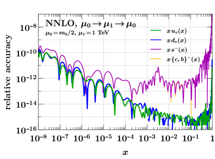
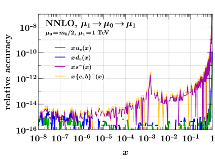
We have also repeated our exercise with the widely-used RK4 method and $h=0.03$, which requires approximately the same number of function calls as DOPRI8 with $h=0.1$ (see the appendix for more detail). This yields relative errors that are orders of magnitude larger for both evolution paths, but still below $10^{-5}$ for $x\leq 0.9$ and away from zero crossings. This shows the significant benefit of using Runge-Kutta methods with high order for DGLAP evolution. Nevertheless, even with the standard RK4 method, we find no indication for numerical instabilities of backward evolution in our setup.

Finally, we note that a Runge-Kutta method with less than the 13 stages of DOPRI8 can be useful if one needs to perform evolution in many small steps, for instance when computing jet cross sections with $\mu\sim p_{T}$ for a dense grid in the transverse jet momentum $p_{T}$. Setting $h\sim 0.03$, we find the DOPRI6 method with its 8 stages to be well suited for such situations.

6 Conclusions

We have shown that a global interpolation using high-order Chebyshev polynomials allows for an efficient and highly accurate numerical representation of PDFs. Compared with local interpolation methods on equispaced grids, such as splines, our method can reach much higher numerical accuracies whilst keeping the computational cost at a comparable or reduced level.

Not only interpolation, but also differentiation and integration of PDFs are numerically accurate and computationally simple in our approach. The same holds for the Mellin convolution of a PDF with an integral kernel, which can be implemented as a simple multiplication with a pre-computed matrix. In particular, high accuracy is retained if the kernel has a strong singularity at the integration end point, such as $\bigl{[}\ln^{5}(1-z)/(1-z)\bigr{]}_{+}$ or $\ln^{4}(1-z)$. Even for such demanding applications, it is possible to achieve a numerical accuracy below $10^{-6}$ with only about $60$ to $70$ grid points. Hence, with our method, numerical inaccuracies become safely negligible for practical physics calculations involving PDFs. If desired, the inaccuracy caused by the interpolation can be estimated with modest additional computational effort by using interpolation on the same grid without the end points. This yields an estimate that is appropriately conservative, but not as overly conservative as the estimate we obtain with Gauss-Kronrod quadrature in the case of integration.

By combining our Chebyshev-based interpolation with a Runge-Kutta method of high order, we obtain a very accurate implementation of DGLAP evolution. Using 70 grid points in $x$ and evolving from $\mu=1.41\,\mathrm{GeV}$ to $\mu=10\,\mathrm{TeV}$, we find relative errors below $10^{-7}$ for $x$ between $10^{-7}$ and $0.8$. We successfully tested our implementation against the benchmark evolution tables in refs. [73, 74]. Performing backward evolution with our method, we find no indications for any numerical instabilities.

Let us briefly point out differences between our implementation of Chebyshev interpolation and the use of Chebyshev polynomials in parameterizations of PDFs. Perhaps most striking is that the order of the highest polynomial used is much larger in our case. There are several reasons for this. First, our approach aims at keeping uncertainties due to interpolation small compared to physics uncertainties. By contrast, as argued in [13], a PDF parameterization need not be much more accurate (relative to the unknown true form) than the uncertainty resulting from fitting the PDFs to data. Second, as we have seen, polynomials up to order 20 or 40 can be handled with ease in our method, whereas PDF determinations naturally tend to limit the number of parameters to be fitted to data. Third, the detailed functional forms used in the PDF parameterizations refs. [11, 12, 13, 14] at a fixed scale $\mu$ differ from each other and from the form (3.2) we use for interpolation at any scale $\mu$. It may be interesting to further investigate the impact of these differences on the number of polynomials required for a satisfactory description of PDFs.

Our approach is implemented in the C++ library ChiliPDF, which is still under development and which we plan to eventually make public. To give a sense of its current performance, we note that the evaluation of the interpolated PDF takes less than a microsecond. With the settings in section 5.2, NNLO DGLAP evolution from $\mu=1.41\,\mathrm{GeV}$ to $\mu=100\,\mathrm{GeV}$ at $n_{F}=4$ takes on the order of 10 to 20 milliseconds. If significantly faster access to evolved PDFs is needed, it may be preferable to pre-compute the $\mu$ dependence and use interpolation in both $x$ and $\mu$. This can easily be done using the techniques we have described.

To conclude, let us mention additional features that are already available in ChiliPDF but not discussed here: $(i)$ polarized evolution up to NNLO for longitudinal and up to NLO for transverse and linear polarizations, with flavor matching up to NLO for all cases, $(ii)$ combined QCD and QED evolution of PDFs with kernels up to $\mathcal{O}(\alpha_{s}\mskip 1.5mu\alpha)$ and $\mathcal{O}(\alpha^{2})$, with QED flavor matching up to $\mathcal{O}(\alpha)$, and $(iii)$ evolution and flavor matching of double parton distributions $F(x_{1},x_{2},\vec{y}\mskip 1.5mu;\mu_{1},\mu_{2})$. For the latter, accuracy goals are typically lower than for computations involving PDFs, but the possibility to work with a low number of grid points is crucial for keeping memory requirements manageable. This will be described in a future paper.

Appendix A Runge-Kutta methods

In this appendix, we take a closer look at the Runge-Kutta (RK) algorithm, which we use to solve the discretized DGLAP equation (5.2), as well as the renormalization group equation (5.4) for the running coupling. We pay special attention to different Runge-Kutta methods and their accuracy.

The RK algorithm solves the initial value problem

$$\mathrm{d}y(t)/\mathrm{d}t =F(t,y) \text{with~{}~{}}y(t_{0}) =y_{0}\,.$$ (A.1)

It approximates the solution $y(t)$ by the set of values $y_{i}\approx y(t_{i})$ at equispaced points $t_{i}$. The distance between two consecutive points is called the step size $h=t_{i+1}-t_{i}$, and the algorithm computes $y_{i+1}$ from the approximate solution $y_{i}$ at the previous point. The solution at a given $t_{f}$ is obtained by dividing the interval $[t_{0},t_{f}]$ into $N$ steps, such that $t_{f}=t_{N}$. When using the algorithm in our work, we fix a maximum step size $h_{\text{max}}$. For any given $t_{0}$ and $t_{f}$, the number of steps is then taken as the smallest integer $N$ that satisfies $|t_{f}-t_{0}|/N\leq h_{\text{max}}$. For brevity, $h_{\text{max}}$ is denoted by $h$ in section 5.

In so-called explicit RK methods, the algorithm for a step is of the form

$$y_{i+1}=y_{i}+h\sum_{j=1}^{s}b_{j}\mskip 1.5muk_{j}$$ (A.2)

with

$$k_{1} =F(t_{i},\mskip 1.5muy_{i})\,,$$

$$k_{2} =F(t_{i}+h\mskip 1.5muc_{2},\mskip 1.5muy_{i}+h\mskip 1.5mua_{21}\mskip 1.5muk_{1})\,,$$

$$k_{3} =F\bigl{(}t_{i}+h\mskip 1.5muc_{3},\mskip 1.5muy_{i}+h\mskip 1.5mu[a_{31}\mskip 1.5muk_{1}+a_{32}\mskip 1.5muk_{2}]\mskip 1.5mu\bigr{)}\,,$$

$$\vdots$$

$$k_{s} =F\bigl{(}t_{i}+h\mskip 1.5muc_{s},\mskip 1.5muy_{i}+h\mskip 1.5mu[a_{s1}\mskip 1.5muk_{1}+\dots+a_{s,s-1}\mskip 1.5muk_{s-1}]\mskip 1.5mu\bigr{)}\,.$$ (A.3)

In standard nomenclature, one calls $s$ the number of stages, $a_{ij}$ the RK matrix, $b_{i}$ the weights and $c_{i}$ the nodes. Different RK methods are characterized by different values of these parameters.

A method is of order $p$ if a single step has a numerical accuracy of $\mathcal{O}(h^{p+1})$. For a given set of RK parameters, it is easy to determine $p$ from eqs. (A.2) and (A) by a Taylor expansion in $h$. Since for given $t_{0}$ and $t_{f}$ the number of required steps scales like $1/h$, the cumulated numerical error of $N$ steps in the solution of the initial value problem (A.1) is

$$y_{N}=y(t_{f})+\mathcal{O}(h^{p})\,.$$ (A.4)

A broad range of RK methods with different orders and numbers of stages is known [77]. Widely used is the RK4 method, also called the “classic RK method” or simply “the RK method”, which has four stages and order $p=4$. We also investigate several methods with $p>4$, one by Cash and Karp [78] and three by Dormand and Prince [79, 80]. According to their order, we denote the latter by DOPRI5, DOPRI6, and DOPRI8. The main parameters of these methods are given in table 4. As noted in ref. [80], the order of the DOPRI6 method is 7 rather than 6 if the function $F(t,y)$ in eq. (A.1) has no explicit $t$ dependence. The numerical study described below suggests that the DOPRI8 method is of order 10 if $F(t,y)$ is $t$ independent. We do not attempt to provide a general proof for this conjecture and hence put a question mark next to the corresponding entry in our table.

method	RK4	Cash-Karp	DOPRI5	DOPRI6	DOPRI8
order $(p)$	4	5	5	6(7)	8(10?)
stages $(s)$	4	6	7	8	13

Table 4: Order and number of stages of the different Runge-Kutta methods investigated in this work. The entries in parentheses are explained in the text.

To quantify the performance of the different methods for DGLAP evolution, we evolve the sample PDF $f_{1}(x)$ given in eq. (3.1) with the DGLAP kernel for the flavor non-singlet combination $u^{+}-d^{\mskip 1.5mu+}$, either at LO or at NLO. As can be seen in eqs. (5.5) and (5.6), LO evolution corresponds to a $t$ independent function $F(t,y)$, whereas NLO evolution implies an explicit $t$ dependence in $F(t,y)$. We evolve from $t_{0}=0.7$ to $t_{f}=1.7$. According to eq. (5.3), this respectively gives $\alpha_{s}\approx 0.5$ and $\alpha_{s}\approx 0.18$, so that the $t$ dependence of $F(t,y)$ for NLO evolution is quite strong at the lower end of the evolution interval.

To monitor the accuracy of evolution, we consider either the evolved PDF at a given $x$ or the truncated Mellin moment (3.7) with a given moment index $j$. The results are similar in both cases. In figure -105, we show the accuracy for the moment with $j=3$ as a function of $N_{\text{fc}}=s\mskip 1.5muN_{\text{steps}}$, where $s$ is the number of stages of the RK method and $N_{\text{steps}}$ the number of RK steps between $t_{0}$ to $t_{f}$. Hence, $N_{\text{fc}}$ is the total number of calls to the function $F(t,y)$ during evolution. The accuracy is determined from the difference between the solution at the selected $N_{\text{fc}}$ and the solution at a value of $N_{\text{fc}}$ in the region where the result does not significantly change any more.

Figure -105: Relative accuracy of different Runge-Kutta methods as a function of the total number $N_{\text{fc}}=s\mskip 1.5muN_{\text{steps}}$ of calls to the function $F(t,y)$ in eq. (A.1). The accuracy is evaluated for the truncated Mellin moment $M(j)$ of the sample PDF $f_{1}(x)$, evolved from $t_{0}=0.7$ to $t_{f}=1.7$. The lines connecting the points correspond to a fitted power law $(N_{\text{fc}})^{-p}$ with $p$ reported in the legend.

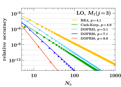
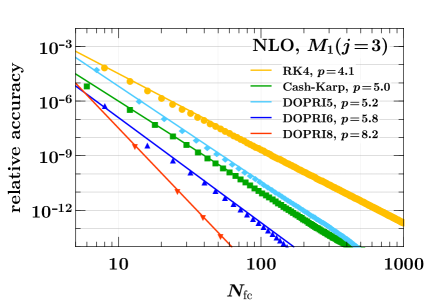
For each RK method, we can identify a region in which the accuracy follows a power law $(N_{\text{fc}})^{-p}$. We determine the corresponding value $p$ by a fit and find it in reasonable agreement with the order of the method. This indicates that in the corresponding region of $N_{\text{fc}}$ the error estimate in eq. (A.4) is indeed applicable.

Our investigation shows the significant advantage of RK methods with high order $p$ for solving the DGLAP equations. For the example shown in the figure, the DOPRI8 method yields a relative accuracy below $10^{-8}$ with a single step (corresponding to 13 function calls), and the limits of machine precision are reached with 50 to 100 function calls.

A similar conclusion can be drawn for the computation of $\alpha_{s}(\mu)$ from eq. (5.4). To illustrate this, we evolve $\alpha_{s}(M_{Z})=0.118$ down to $\mu_{0}=2.25\,\mathrm{GeV}$ with $n_{F}=5$. We use the DOPRI8 method and impose a maximum step size $h_{\text{max}}=0.2$. The evolved value $\alpha_{s}(\mu_{0})$ is then inserted into the exact analytic expression of $\mu(\alpha_{s})$ at the appropriate perturbative order. Both at NLO and at NNLO, we find that the resulting value of $\mu$ agrees with $\mu_{0}$ at the level of $2\times 10^{-15}$.

References

- [1] A. Buckley, J. Ferrando, S. Lloyd, K. Nordström, B. Page, M. Rüfenacht et al., LHAPDF6: parton density access in the LHC precision era, Eur. Phys. J. C75 (2015) 132 [1412.7420].
- [2] F. J. Yndurain, Reconstruction of the Deep Inelastic Structure Functions from their Moments, Phys. Lett. B 74 (1978) 68.
- [3] G. Parisi and N. Sourlas, A Simple Parametrization of the Dependence of the Quark Distributions in QCD, Nucl. Phys. B 151 (1979) 421.
- [4] W. Furmanski and R. Petronzio, A Method of Analyzing the Scaling Violation of Inclusive Spectra in Hard Processes, Nucl. Phys. B 195 (1982) 237.
- [5] R. Kobayashi, M. Konuma and S. Kumano, FORTRAN program for a numerical solution of the nonsinglet Altarelli-Parisi equation, Comput. Phys. Commun. 86 (1995) 264 [hep-ph/9409289].
- [6] J. Chyla and J. Rames, On Methods of Analyzing Scaling Violation in Deep Inelastic Scattering, Z. Phys. C 31 (1986) 151.
- [7] J. Blümlein, M. Klein, G. Ingelman and R. Rückl, Testing QCD Scaling Violations in the HERA Energy Range, Z. Phys. C 45 (1990) 501.
- [8] V. G. Krivokhizhin, S. P. Kurlovich, R. Lednicky, S. Nemecek, V. V. Sanadze, I. A. Savin et al., Next-to-leading order QCD analysis of structure functions with the help of Jacobi polynomials, Z. Phys. C 48 (1990) 347.
- [9] M. Bonvini, S. Forte and G. Ridolfi, Soft gluon resummation of Drell-Yan rapidity distributions: Theory and phenomenology, Nucl. Phys. B 847 (2011) 93 [1009.5691].
- [10] M. Bonvini and S. Marzani, Resummed Higgs cross section at N3LL, JHEP 09 (2014) 007 [1405.3654].
- [11] J. Pumplin, Parametrization dependence and in parton distribution fitting, Phys. Rev. D 82 (2010) 114020 [0909.5176].
- [12] A. Glazov, S. Moch and V. Radescu, Parton Distribution Uncertainties using Smoothness Prior, Phys. Lett. B 695 (2011) 238 [1009.6170].
- [13] A. D. Martin, A. J. T. M. Mathijssen, W. J. Stirling, R. S. Thorne, B. J. A. Watt and G. Watt, Extended Parameterisations for MSTW PDFs and their effect on Lepton Charge Asymmetry from W Decays, Eur. Phys. J. C 73 (2013) 2318 [1211.1215].
- [14] L. A. Harland-Lang, A. D. Martin, P. Motylinski and R. S. Thorne, Parton distributions in the LHC era: MMHT 2014 PDFs, Eur. Phys. J. C75 (2015) 204 [1412.3989].
- [15] F. Dulat, B. Mistlberger and A. Pelloni, Differential Higgs production at N3LO beyond threshold, JHEP 01 (2018) 145 [1710.03016].
- [16] M. Miyama and S. Kumano, Numerical solution of evolution equations in a brute force method, Comput. Phys. Commun. 94 (1996) 185 [hep-ph/9508246].
- [17] P. G. Ratcliffe, A matrix approach to numerical solution of the DGLAP evolution equations, Phys. Rev. D 63 (2001) 116004 [hep-ph/0012376].
- [18] C. Pascaud and F. Zomer, A Fast and precise method to solve the Altarelli-Parisi equations in x space, hep-ph/0104013.
- [19] M. Dasgupta and G. Salam, Resummation of the jet broadening in DIS, Eur. Phys. J. C 24 (2002) 213 [hep-ph/0110213].
- [20] NNPDF collaboration, L. Del Debbio, S. Forte, J. I. Latorre, A. Piccione and J. Rojo, Neural network determination of parton distributions: The Nonsinglet case, JHEP 03 (2007) 039 [hep-ph/0701127].
- [21] S. Weinzierl, Fast evolution of parton distributions, Comput. Phys. Commun. 148 (2002) 314 [hep-ph/0203112].
- [22] A. Vogt, Efficient evolution of unpolarized and polarized parton distributions with QCD-PEGASUS, Comput. Phys. Commun. 170 (2005) 65 [hep-ph/0408244].
- [23] A. Candido, F. Hekhorn and G. Magni, EKO: Evolution Kernel Operators, 2202.02338.
- [24] A. Cafarella, C. Coriano and M. Guzzi, Precision Studies of the NNLO DGLAP Evolution at the LHC with CANDIA, Comput. Phys. Commun. 179 (2008) 665 [0803.0462].
- [25] G. P. Salam and J. Rojo, A Higher Order Perturbative Parton Evolution Toolkit (HOPPET), Comput. Phys. Commun. 180 (2009) 120 [0804.3755].
- [26] M. Botje, QCDNUM: Fast QCD Evolution and Convolution, Comput. Phys. Commun. 182 (2011) 490 [1005.1481].
- [27] V. Bertone, S. Carrazza and J. Rojo, APFEL: A PDF Evolution Library with QED corrections, Comput. Phys. Commun. 185 (2014) 1647 [1310.1394].
- [28] V. Bertone, APFEL++: A new PDF evolution library in C++, PoS DIS2017 (2018) 201 [1708.00911].
- [29] M. Procura, W. J. Waalewijn and L. Zeune, Resummation of Double-Differential Cross Sections and Fully-Unintegrated Parton Distribution Functions, JHEP 02 (2015) 117 [1410.6483].
- [30] G. Lustermans, J. K. L. Michel, F. J. Tackmann and W. J. Waalewijn, Joint two-dimensional resummation in and -jettiness at NNLL, JHEP 03 (2019) 124 [1901.03331].
- [31] G. Lustermans, J. K. L. Michel and F. J. Tackmann, Generalized Threshold Factorization with Full Collinear Dynamics, 1908.00985.
- [32] J. R. Gaunt and M. Stahlhofen, The Fully-Differential Quark Beam Function at NNLO, JHEP 12 (2014) 146 [1409.8281].
- [33] J. R. Gaunt and M. Stahlhofen, The fully-differential gluon beam function at NNLO, JHEP 07 (2020) 234 [2004.11915].
- [34] A. Hornig, D. Kang, Y. Makris and T. Mehen, Transverse Vetoes with Rapidity Cutoff in SCET, JHEP 12 (2017) 043 [1708.08467].
- [35] J. K. L. Michel, P. Pietrulewicz and F. J. Tackmann, Jet Veto Resummation with Jet Rapidity Cuts, JHEP 04 (2019) 142 [1810.12911].
- [36] M. Bonvini, A. S. Papanastasiou and F. J. Tackmann, Resummation and matching of b-quark mass effects in production, JHEP 11 (2015) 196 [1508.03288].
- [37] P. Pietrulewicz, D. Samitz, A. Spiering and F. J. Tackmann, Factorization and Resummation for Massive Quark Effects in Exclusive Drell-Yan, JHEP 08 (2017) 114 [1703.09702].
- [38] I. Moult, L. Rothen, I. W. Stewart, F. J. Tackmann and H. X. Zhu, Subleading Power Corrections for N-Jettiness Subtractions, Phys. Rev. D 95 (2017) 074023 [1612.00450].
- [39] I. Moult, L. Rothen, I. W. Stewart, F. J. Tackmann and H. X. Zhu, N -jettiness subtractions for at subleading power, Phys. Rev. D 97 (2018) 014013 [1710.03227].
- [40] M. A. Ebert, I. Moult, I. W. Stewart, F. J. Tackmann, G. Vita and H. X. Zhu, Power Corrections for N-Jettiness Subtractions at , JHEP 12 (2018) 084 [1807.10764].
- [41] R. Boughezal, X. Liu and F. Petriello, Power Corrections in the N-jettiness Subtraction Scheme, JHEP 03 (2017) 160 [1612.02911].
- [42] R. Boughezal, A. Isgrò and F. Petriello, Next-to-leading-logarithmic power corrections for -jettiness subtraction in color-singlet production, Phys. Rev. D 97 (2018) 076006 [1802.00456].
- [43] A. Bhattacharya, I. Moult, I. W. Stewart and G. Vita, Helicity Methods for High Multiplicity Subleading Soft and Collinear Limits, JHEP 05 (2019) 192 [1812.06950].
- [44] M. A. Ebert, I. Moult, I. W. Stewart, F. J. Tackmann, G. Vita and H. X. Zhu, Subleading power rapidity divergences and power corrections for qT, JHEP 04 (2019) 123 [1812.08189].
- [45] R. D. Ball, E. R. Nocera and J. Rojo, The asymptotic behaviour of parton distributions at small and large , Eur. Phys. J. C 76 (2016) 383 [1604.00024].
- [46] M. Diehl and J. R. Gaunt, Double parton scattering theory overview, Adv. Ser. Direct. High Energy Phys. 29 (2018) 7 [1710.04408].
- [47] S. Carrazza, J. M. Cruz-Martinez and M. Rossi, PDFFlow: Parton distribution functions on GPU, Comput. Phys. Commun. 264 (2021) 107995 [2009.06635].
- [48] C. Runge, Über empirische Funktionen und die Interpolation zwischen äquidistanten Ordinaten, Z. Math. Phys. 46 (1901) 224.
- [49] L. N. Trefethen, “Six Myths of Polynomial Interpolation and Quadrature.” https://people.maths.ox.ac.uk/trefethen/mythspaper.pdf, 2011.
- [50] L. N. Trefethen, Approximation Theory and Approximation Practice. Society for Industrial and Applied Mathematics, 2012.
- [51] L. N. Trefethen, Is Gauss Quadrature Better than Clenshaw–Curtis?, SIAM Review 50 (2008) 67.
- [52] J. Waldvogel, Fast Construction of the Fejér and Clenshaw–Curtis Quadrature Rules, Bit Numer. Math. 46 (2006) 195.
- [53] Gauss-Kronrod quadrature formula, in Encyclopedia of Mathematics, https://www.encyclopediaofmath.org/index.php/Gauss-Kronrod_quadrature_formula.
- [54] T. N. L. Patterson, The optimum addition of points to quadrature formulae, Math. Comp. 22 (1968) 847.
- [55] S. Alekhin, J. Blümlein, S. Moch and R. Placakyte, Parton distribution functions, , and heavy-quark masses for LHC Run II, Phys. Rev. D96 (2017) 014011 [1701.05838].
- [56] H1, ZEUS collaboration, H. Abramowicz et al., Combination of measurements of inclusive deep inelastic scattering cross sections and QCD analysis of HERA data, Eur. Phys. J. C75 (2015) 580 [1506.06042].
- [57] P. Jimenez-Delgado and E. Reya, Delineating parton distributions and the strong coupling, Phys. Rev. D89 (2014) 074049 [1403.1852].
- [58] NNPDF collaboration, R. D. Ball et al., Parton distributions from high-precision collider data, Eur. Phys. J. C 77 (2017) 663 [1706.00428].
- [59] T.-J. Hou et al., New CTEQ global analysis of quantum chromodynamics with high-precision data from the LHC, Phys. Rev. D 103 (2021) 014013 [1912.10053].
- [60] S. Bailey, T. Cridge, L. A. Harland-Lang, A. D. Martin and R. S. Thorne, Parton distributions from LHC, HERA, Tevatron and fixed target data: MSHT20 PDFs, Eur. Phys. J. C 81 (2021) 341 [2012.04684].
- [61] R. D. Ball et al., The Path to Proton Structure at One-Percent Accuracy, 2109.02653.
- [62] S. Dulat, T.-J. Hou, J. Gao, M. Guzzi, J. Huston, P. Nadolsky et al., New parton distribution functions from a global analysis of quantum chromodynamics, Phys. Rev. D 93 (2016) 033006 [1506.07443].
- [63] A. Vogt, S. Moch and J. A. M. Vermaseren, The Three-loop splitting functions in QCD: The Singlet case, Nucl. Phys. B691 (2004) 129 [hep-ph/0404111].
- [64] J. Ablinger, A. Behring, J. Blümlein, A. De Freitas, A. von Manteuffel and C. Schneider, The three-loop splitting functions and , Nucl. Phys. B 922 (2017) 1 [1705.01508].
- [65] NNPDF collaboration, R. D. Ball et al., Parton distributions for the LHC Run II, JHEP 04 (2015) 040 [1410.8849].
- [66] Y. L. Dokshitzer, Calculation of the Structure Functions for Deep Inelastic Scattering and e+ e- Annihilation by Perturbation Theory in Quantum Chromodynamics., Sov. Phys. JETP 46 (1977) 641.
- [67] V. N. Gribov and L. N. Lipatov, Deep inelastic e p scattering in perturbation theory, Sov. J. Nucl. Phys. 15 (1972) 438.
- [68] G. Altarelli and G. Parisi, Asymptotic Freedom in Parton Language, Nucl. Phys. B126 (1977) 298.
- [69] S. Moch, J. A. M. Vermaseren and A. Vogt, The Three loop splitting functions in QCD: The Nonsinglet case, Nucl. Phys. B688 (2004) 101 [hep-ph/0403192].
- [70] K. Chetyrkin, B. A. Kniehl and M. Steinhauser, Strong coupling constant with flavor thresholds at four loops in the MS scheme, Phys. Rev. Lett. 79 (1997) 2184 [hep-ph/9706430].
- [71] M. Buza, Y. Matiounine, J. Smith and W. van Neerven, Charm electroproduction viewed in the variable flavor number scheme versus fixed order perturbation theory, Eur. Phys. J. C 1 (1998) 301 [hep-ph/9612398].
- [72] A. Behring, I. Bierenbaum, J. Blümlein, A. De Freitas, S. Klein and F. Wißbrock, The logarithmic contributions to the asymptotic massive Wilson coefficients and operator matrix elements in deeply inelastic scattering, Eur. Phys. J. C 74 (2014) 3033 [1403.6356].
- [73] W. Giele et al., The QCD / SM working group: Summary report, in Physics at TeV colliders. Proceedings, Euro Summer School, Les Houches, France, May 21-June 1, 2001, pp. 275–426, 2002, hep-ph/0204316.
- [74] M. Dittmar et al., Working Group I: Parton distributions: Summary report for the HERA LHC Workshop Proceedings, hep-ph/0511119.
- [75] G. P. Salam and A. Vogt, private communication.
- [76] E. Ruiz Arriola, NLO evolution for large scale distances, positivity constraints and the low-energy model of the nucleon, Nucl. Phys. A 641 (1998) 461.
- [77] E. Hairer, S. P. Nørsett and G. Wanner, Solving Ordinary Differential Equations I: Nonstiff Problems. Springer-Verlag, 1993.
- [78] J. R. Cash and A. H. Karp, A variable order runge-kutta method for initial value problems with rapidly varying right-hand sides, ACM Trans. Math. Softw. 16 (1990) 201.
- [79] J. Dormand and P. Prince, A family of embedded runge-kutta formulae, Journal of Computational and Applied Mathematics 6 (1980) 19 .
- [80] P. Prince and J. Dormand, High order embedded runge-kutta formulae, Journal of Computational and Applied Mathematics 7 (1981) 67 .