A Formal Model for Polarization
under Confirmation Bias in Social Networks

Abstract.

We describe a model for polarization in multi-agent systems based on Esteban and Ray’s standard family of polarization measures from economics. Agents evolve by updating their beliefs (opinions) based on an underlying influence graph, as in the standard DeGroot model for social learning, but under a confirmation bias; i.e., a discounting of opinions of agents with dissimilar views. We show that even under this bias polarization eventually vanishes (converges to zero) if the influence graph is strongly-connected. If the influence graph is a regular symmetric circulation, we determine the unique belief value to which all agents converge. Our more insightful result establishes that, under some natural assumptions, if polarization does not eventually vanish then either there is a disconnected subgroup of agents, or some agent influences others more than she is influenced. We also prove that polarization does not necessarily vanish in weakly-connected graphs under confirmation bias. Furthermore, we show how our model relates to the classic DeGroot model for social learning. We illustrate our model with several simulations of a running example about polarization over vaccines and of other case studies. The theoretical results and simulations will provide insight into the phenomenon of polarization.

1. Introduction

Distributed systems have changed significantly with the advent of social networks. In the previous incarnation of distributed computing [Lyn96], the emphasis was on consistency, fault tolerance, resource management, and related topics; these were all characterized by interaction between processes. The new era of distributed systems adds an emphasis on the flow of epistemic information (facts, beliefs, lies) and its impact on democracy and on society at large.

Social networks may facilitate civil discourse by enabling a prompt exchange of facts, beliefs and opinions among members of a community. Nevertheless, users in social networks may shape their beliefs by attributing more value to the opinions of influential figures. This common cognitive bias is known as authority bias [Ram19]. Furthermore, social networks often target their users with information that they may already agree with to keep engagement. It is known that users tend to give more value to opinions that confirm their own preexisting beliefs [AWA10] in another common cognitive bias known as confirmation bias. As a result, social networks can cause their users to become radical and isolated in their own ideological circle, potentially leading to dangerous splits in society [Boz13] in a phenomenon known as polarization [AWA10].

Indeed, social media platforms have played a key role in the polarization of political processes. Referenda such as Brexit and the Colombian Peace Agreement, as well as recent presidential elections in Brazil and USA are compelling examples of this phenomenon [Kir17]. These cases illustrate that messages in social media with elements of extremist ideology in political and public discourse may cause polarization and negatively influence fundamental decision-making processes.

Consequently, we believe that developing a model that focuses on central aspects in social networks, such as influence graphs and evolution of users’ beliefs, represents a significant contribution to the understanding of the phenomenon of polarization. In fact, there is a growing interest in the development of models for the analysis of polarization and social influence in networks [LSSZ13, PMC16, SPGK18, GG16, Eld19, CGMJCK13, Ped, DeG74, GJ10, Chr16, SLG11, SLG13, Hun17]. Since polarization involves non-terminating systems with multiple agents simultaneously exchanging information (opinions), concurrency models are a natural choice to capture the dynamics of this phenomenon.

Our approach

In this paper we present a multi-agent model for polarization inspired by linear-time models of concurrency where the state of the system evolves in discrete time units (in particular [SJG94, NPV02, Val01]). In each time unit, the users, called agents, update their beliefs about a given proposition of interest by taking into account the beliefs of their neighbors through an underlying weighted influence graph. The belief update gives more value to the opinion of agents with higher influence (authority bias) and to the opinion of agents with similar views (confirmation bias). Furthermore, the model is equipped with a polarization measure based on the seminal work in economics by Esteban and Ray [ER94]. Polarization is measured at each time unit and it is zero if all agents’ beliefs fall within an interval of agreement about the proposition.

Our goal is to explore how the combination of influence graphs and cognitive biases in our model can lead to polarization. The closest related work is that on DeGroot models [DeG74]. These are the standard linear models for social learning whose analyses can be carried out by standard linear techniques from Markov chains. Nevertheless, a novelty in our model is that its update function extends the classical update from DeGroot models with confirmation bias. As we elaborate in Section 6.1, the extension makes the model no longer linear and thus mathematical tools like Markov chains are not applicable in a straightforward way. Our model also incorporates a polarization measure in a model for social learning and extends the classical convergence results of DeGroot models to the confirmation bias case.

Main Contributions

We introduce a variant of the standard DeGroot model where agents can update their beliefs under confirmation bias. By employing techniques from calculus, graph theory, and flow networks, we identify how networks and beliefs are structured, for agents subject to confirmation bias, when polarization does not disappear. Furthermore, we illustrate and discuss some perhaps unexpected aspects of the temporal evolution of polarization by means of a series of elucidating simulations. In particular, we address the non-monotonic evolution of polarization as well as the effect on polarization of various update functions, influence graphs, and initial belief configurations among agents.

The following are our main theoretical contributions. Assuming confirmation bias and some natural conditions about the initial belief values, we show that:

1. Polarization eventually disappears (converges to zero) if the influence graph is strongly-connected (Definition 4.2).

2. If polarization does not disappear then either there is a disconnected subgroup of agents (i.e., the influence graph is not weakly connected, see Definition 17), or some agent influences others more than she is influenced, or all the agents are initially radicalized (i.e., each individual holds the most extreme value either in favor or against the given proposition of interest).

3. If the influence graph is a regular symmetric circulation (Section 5.3) we determine the unique belief value all agents converge to.

An implementation in Python of the model and the corresponding simulations presented in this paper are publicly available on GitHub [AAK⁺21].

All in all, our formal model, theoretical results, and experimental observations provide insight into the phenomenon of polarization, and are a step toward the design of robust computational models and simulation software for human cognitive and social processes.

Organization

In Section˜2 we introduce our formal model, and in Section 3 we provide a series of examples and simulations uncovering interesting new insights and complex characteristics of the evolution of beliefs and polarization under confirmation bias. The first contribution listed above appears in Section 4 while the other two appear in Section 5. We discuss DeGroot and other related work in Section 6, and conclude in Section 7. For the sake of readability, the proofs follow in Appendix B.

2. The Model

Here we present our polarization model, which is composed of “static” and “dynamic” elements. We presuppose basic knowledge of calculus and graph theory [Soh14, Die17].

2.1. Static Elements of the Model

Static elements of the model represent a snapshot of a social network at a given point in time. They include the following components:

• A (finite) set $\mathcal{A}=\{0,1,\ldots,n{-}1\}$ of $n\geq 1$ agents.

• A proposition $p$ representing a declarative sentence, proposing something as being true. We shall refer to $p$ as a statement or proposition. For example $p$ could be the statement “vaccines are safe”, “Brexit was a mistake”, or “climate change is real and is caused by human activity”. We shall see next how each agent in $\mathcal{A}$ assigns a value to $p$. The sentence $p$ is atomic in the sense that the value assigned to $p$ is obtained from $p$ as a whole; i.e., it is not obtained by composing values assigned to other sentences.

• A belief configuration $B:\mathcal{A}\rightarrow[0,1]$ such that for each agent $i\in\mathcal{A}$, the value $B_{i}=B(i)$ represents the confidence of agent $i\in\mathcal{A}$ in the veracity of proposition $p$. The higher the value $B_{i}$, the higher the confidence of agent $i$ in the veracity of $p$. Extreme values $0$ and $1$ represent a firm belief of agent $i$ in, respectively, the falsehood or truth of $p$. A belief configuration $B$ can also be represented as a tuple $(B_{0},\ldots,B_{n-1})$. Given the set of agents $\mathcal{A}$, we use $[0,1]^{\mathcal{A}}$ to denote the set all belief configurations over $\mathcal{A}$.

• A polarization measure $\rho:[0,1]^{\mathcal{A}}\rightarrow\mathbb{R}^{+}$ mapping belief configurations to the non-negative real numbers. Given a belief configuration $B=(B_{0},\ldots,B_{n-1})$, the value $\rho(B)$ indicates the polarization among all the agents in $\mathcal{A}$ given their beliefs $B_{0},\ldots,B_{n-1}$ about the veracity of the statement $p$. The higher the value $\rho(B)$, the higher the polarization amongst the agents in $\mathcal{A}$.

There are several polarization measures described in the literature. In this work we employ the influential family of measures proposed by Esteban and Ray [ER94].

In the rest of the paper, we will use the following notion. We say that $(\pi,y)=(\pi_{0},\allowbreak\pi_{1},\allowbreak\ldots,\allowbreak\pi_{k{-}1},\allowbreak y_{0},\allowbreak y_{1},\allowbreak\ldots,\allowbreak y_{k{-}1})$ is a distribution if $y\in\mathbb{R}^{k}$, $\sum_{i=0}^{k-1}\pi_{i}=1$ and for every $i,j$ we have $\pi_{i}\geq 0$ and $y_{i}\neq y_{j}$ whenever $j\neq i$. We use $\mathcal{D}$ to denote the set of all distributions.

[Esteban-Ray Polarization, [ER94]] An Esteban-Ray polarization measure is a mapping $\rho_{\mathit{ER}}:\mathcal{D}\allowbreak\mathrel{\mathop{\hbox to11.99998pt{\rightarrowfill}}\limits}\mathbb{R}^{+}$ for which there are constants $K>0$ and $\alpha\in(0,2)$ such that for every $(\pi,y)=(\pi_{0},\allowbreak\pi_{1},\allowbreak\ldots,\allowbreak\pi_{k{-}1},\allowbreak y_{0},\allowbreak y_{1},\allowbreak\ldots,\allowbreak y_{k{-}1})\in\mathcal{D}$ we have

$$\rho_{\mathit{ER}}(\pi,y)=K\sum_{i=0}^{k-1}\sum_{j=0}^{k-1}\pi_{i}^{1+\alpha}\pi_{j}|y_{i}-y_{j}|.$$

The higher the value of $\rho_{\mathit{ER}}(\pi,y)$, the more polarized distribution $(\pi,y)$ is. The measure captures the intuition that polarization is accentuated by both intra-group homogeneity and inter-group heterogeneity. Moreover, it assumes that the total polarization is the sum of the effects of individual agents on one another. This measure (family) can be derived from a set of intuitively reasonable axioms [ER94], which are presented in Appendix A. Succinctly, the measure considers a society as highly polarized when agents can be divided into two clusters of similar size, one in which everyone has a high level of confidence in the veracity of the proposition, and the other in which everyone has a low level of confidence in the veracity of that same proposition. On the other hand, the measure considers a society as not polarized at all when all individuals share a similar level of belief, and considers it as slightly polarized when all individuals hold different levels of belief, without forming distinctive clusters of similar opinions (i.e., the spread of opinions is diffuse.)

Note that $\rho_{\mathit{ER}}$ is defined on a discrete distribution, whereas in our model a general polarization metric is defined on a belief configuration $B:\mathcal{A}\rightarrow[0,1]$. To apply $\rho_{\mathit{ER}}$ to our setup in [AKV19] we converted the belief configuration $B$ into an appropriate distribution $(\pi,y)$.

First we need some notation: Let $D_{k}$ be a discretization of the interval $[0,1]$ into $k>0$ consecutive non-overlapping, non-empty intervals (bins) $I_{0},I_{1},\ldots,I_{k-1}$. We use the term borderline points of $D_{k}$ to refer to the end-points of $I_{0},I_{1},\ldots,I_{k-1}$ different from 0 and 1. Given a belief configuration $B$, define the belief distribution of $B$ in $D_{k}$ as $\mathbf{bd}(B,D_{k})=(\pi_{0},\allowbreak\pi_{1},\allowbreak\ldots,\allowbreak\pi_{k{-}1},\allowbreak y_{0},\allowbreak y_{1},\allowbreak\ldots,\allowbreak y_{k{-}1})$ where each $y_{i}$ is the mid-point of $I_{i}$, and $\pi_{i}$ is the fraction of agents having their belief in $I_{i}$.

[$k$-bin polarization, [AKV19]]

An Esteban-Ray polarization measure for belief configurations over $D_{k}$ is a mapping $\rho:[0,1]^{\mathcal{A}}\rightarrow\mathbb{R}^{+}$ such that for some Esteban-Ray polarization measure $\rho_{\mathit{ER}}$, we have

$$\rho(B)=\rho_{\mathit{ER}}(\mathbf{bd}(B,D_{k}))$$

for every belief configuration $B\in[0,1]^{\mathcal{A}}.$

Notice that when there is consensus about the proposition $p$ of interest, i.e., when all agents in belief configuration $B$ hold the same belief value, we have $\rho(B)=0$. This happens exactly when all agents’ beliefs fall within the same bin of the underlying discretization $D_{k}$. The following property is an easy consequence from Definition 2.1 and Definition 2.1.

Proposition 1 (Zero Polarization).

Let $\rho$ be a Esteban-Ray polarization measure for belief configurations over a discretization $D_{k}=I_{0},\ldots,I_{k-1}$. Then $\rho(B)=0$ iff there exists $m\in\{0,\ldots,k{-}1\}$ such that for all $i\in\mathcal{A}$, $B_{i}\in I_{m}$.

2.2. Dynamic Elements of the Model

Dynamic elements formalize the evolution of agents’ beliefs as they interact over time and are exposed to different opinions. They include:

• A time frame

  $$\mathcal{T}{=}\{0,1,2,\ldots\}$$

  representing the discrete passage of time.

• A family of belief configurations

  $$\{B^{t}:\mathcal{A}\rightarrow[0,1]\}_{t\in{\mathcal{T}}}$$

  such that each $B^{t}$ is the belief configuration of agents in $\mathcal{A}$ with respect to proposition $p$ at time step $t\in\mathcal{T}$.

• A weighted directed graph

  $$\mathcal{I}:\mathcal{A}\times\mathcal{A}\rightarrow[0,1].$$

  The value $\mathcal{I}(i,j)$, written $\mathcal{I}_{i,j}$, represents the direct influence that agent $i$ has on agent $j$, or the weight $i$ carries with $j$. A higher value means that agent $j$ will have higher confidence in agent $i$’s opinion and, therefore, will give this opinion more weight when incorporating it into its own. Conversely, $\mathcal{I}_{i,j}$ can also be viewed as the trust or confidence that $j$ has in $i$. We assume that $\mathcal{I}_{i,i}=1$ for every agent $i$, meaning that agents are self-confident. We shall often refer to $\mathcal{I}$ simply as the influence (graph) $\mathcal{I}$.

  We distinguish, however, the direct influence $\mathcal{I}_{i,j}$ that $i$ has on $j$ from the overall effect of $i$ on $j$’s belief. This effect is a combination of various factors, including direct influence, their current opinions, the topology of the influence graph, and how agents reason. This overall effect is captured by the update function below.

• An update function

  $$\mu:(B^{t},\mathcal{I})\mapsto B^{t+1}$$

  mapping belief configuration $B^{t}$ at time $t$ and influence graph $\mathcal{I}$ to new belief configuration $B^{t+1}$ at time $t+1$. This function models the evolution of agents’ beliefs over time. We adopt the following premises.

1. Agents present some Bayesian reasoning: Agents’ beliefs are updated at every time step by combining their current belief with a correction term that incorporates the new evidence they are exposed to in that step –i.e., other agents’ opinions. More precisely, when agent $j$ interacts with agent $i$, the former affects the latter moving $i$’s belief towards $j$’s, proportionally to the difference $B^{t}_{j}{-}B^{t}_{i}$ in their beliefs. The intensity of the move is proportional to the influence $\mathcal{I}_{j,i}$ that $j$ carries with $i$. The update function produces an overall correction term for each agent as the average of all other agents’ effects on that agent, and then incorporates this term into the agent’s current belief.  The factor $\mathcal{I}_{j,i}$ allows the model to capture authority bias [Ram19], by which agents’ influences on each other may have different intensities (by, e.g., giving higher weight to an authority’s opinion).

2. Agents may be prone to confirmation bias: Agents may give more weight to evidence supporting their current beliefs while discounting evidence contradicting them, independently from its source. This behavior in known in the psychology literature as confirmation bias [AWA10], and is captured in our model as follows.

   When agent $j$ interacts with agent $i$ at time $t$, the update function moves agent $i$’s belief toward that of agent $j$, proportionally to the influence $\mathcal{I}_{j,i}$ of $j$ on $i$, but with a caveat: the move is stronger when $j$’s belief is similar to $i$’s than when it is dissimilar. This is realized below by making the move proportional to what we shall call confirmation-bias factor $\beta^{t}_{i,j}=1-|B^{t}_{j}{-}B^{t}_{i}|$. Clearly, the closer the beliefs of agents $i$ and $j$ at time $t$, the higher the factor $\beta^{t}_{i,j}$.

The premises above are formally captured in the following update-function. As usual, given a set $S$, we shall use $|S|$ to denote the cardinality of $S$.

[Confirmation-bias update function] Let $B^{t}$ be a belief configuration at time $t\in\mathcal{T}$, and $\mathcal{I}$ be an influence graph. The confirmation-bias update-function is the map $\mu^{\textit{CB}}:({B^{t}},{\mathcal{I}})\mapsto B^{t+1}$ with $B^{t+1}$ given by

$$B^{t+1}_{i}=B^{t}_{i}+\frac{1}{|\mathcal{A}_{i}|}\sum_{j\in\mathcal{A}_{i}}\beta^{t}_{i,j}\,\mathcal{I}_{j,i}\,(B^{t}_{j}-B^{t}_{i}),$$ (1)

for every agent $i\in\mathcal{A}$, where $\mathcal{A}_{i}=\{j\in\mathcal{A}\mid\mathcal{I}_{j,i}>0\}$ is the set of neighbors of $i$ and $\beta^{t}_{i,j}=1-|B^{t}_{j}{-}B^{t}_{i}|$ is the confirmation-bias factor of $i$ with respect to $j$ given their beliefs at time $t$.

The expression $\nicefrac{{1}}{{|\mathcal{A}_{i}|}}\sum_{j\in\mathcal{A}_{i}}\beta^{t}_{i,j}\,\mathcal{I}_{j,i}\,(B^{t}_{j}-B^{t}_{i})$ on the right-hand side of Definition 2.2 is a correction term incorporated into agent $i$’s original belief $B^{t}_{i}$ at time $t$. The correction is the average of the effect of each neighbor $j\in\mathcal{A}_{i}$ on agent $i$’s belief at that time step. The value $B^{t+1}_{i}$ is the resulting updated belief of agent $i$ at time $t+1$. By rewriting (1) as $B^{t+1}_{i}=\nicefrac{{1}}{{|\mathcal{A}_{i}|}}\sum_{j\in\mathcal{A}_{i}}\beta^{t}_{i,j}\,\mathcal{I}_{j,i}\,B^{t}_{j}+\left(1-\beta^{t}_{i,j}\,\mathcal{I}_{j,i}\right)B^{t}_{i}$, it is easy to verify that $B^{t+1}_{i}\in[0,1]$, since: (i) we divide the result of the summation by the number of terms; and (ii) each term of the summation also belongs to the interval $[0,1]$, as it is a convex combination of the beliefs of agent $i$’s neighbors at time $t$ and its own belief, both in the interval $[0,1]$.

The confirmation-bias factor $\beta^{t}_{i,j}$ lies in the interval $[0,1]$, and the lower its value, the more agent $i$ discounts the opinion provided by agent $j$ when incorporating it. It is maximum when agents’ beliefs are identical, and minimum when their beliefs are extreme opposites.

Remark 2 (Classical Update: Authority Non-Confirmatory Bias).

In this paper we focus on confirmation-bias update and, unless otherwise stated, assume the underlying function is given by Definition 2.2. Nevertheless, in Sections 5.3 and 6.1 we will consider a classical update $\mu^{C}:({B^{t}},{\mathcal{I}}){\mapsto}B^{t+1}$ that captures non-confirmatory authority-bias and is obtained by replacing the confirmation-bias factor $\beta^{t}_{i,j}$ in Definition 2.2 with 1. That is,

$$B^{t+1}_{i}=B^{t}_{i}+\frac{1}{|\mathcal{A}_{i}|}\sum_{j\in\mathcal{A}_{i}}\mathcal{I}_{j,i}\,(B^{t}_{j}{-}B^{t}_{i}).$$ (2)

We refer to this function as classical because it is closely related to the standard update function of the DeGroot models for social learning from Economics [DeG74]. This correspondence will be formalized in Section 6.1.

Remark 3.

A preliminary and slightly different version of the biases in Definition 2.2 and Remark 2 using in Equations 1 and 2 the set $\mathcal{A}$ instead of $\mathcal{A}_{i}$ were given [AKV19]. As a consequence these preliminary definitions take into account the weighted average of all agents’ beliefs rather that only those of the agents that have an influence over agent $i$.

3. Running Example and Simulations

In this section we present a running example, as well as several simulations, that motivate our theoretical results from the following sections. We start by stating some assumptions that will be adopted throughout this section.

3.1. General assumptions

Recall that we assume $\mathcal{I}_{i,i}=1$ for every $i\in\mathcal{A}$. However, for simplicity, in all figures of influence graphs we omit self-loops. In all cases we limit our analyses to a fixed number of time steps. We compute a polarization measure from Definition 2.1 with parameters $\alpha=1.6$, as suggested by Esteban and Ray [ER94], and $K=1,000$. Moreover, we employ a discretization $D_{k}$ of the interval $[0,1]$ into $k=5$ bins, each representing a possible general position with respect to the veracity of the proposition $p$ of interest:

• strongly against: $[0,0.20)$;

• fairly against: $[0.20,0.40)$;

• neutral/unsure: $[0.40,0.60)$;

• fairly in favour: $[0.60,0.80)$; and

• strongly in favour: $[0.80,1]$.

In all definitions we let $\mathcal{A}=\{0,1,\ldots,n{-}1\}$, and $i,j\in\mathcal{A}$ be generic agents.

3.2. Running example

As a motivating example we consider the following hypothetical situation.

[Vaccine Polarization] Consider the sentence “vaccines are safe” as the proposition $p$ of interest. Assume a set $\mathcal{A}$ of $6$ agents that is initially extremely polarized about $p$: Agents 0 and 5 are absolutely confident, respectively, in the falsehood or truth of $p$, whereas the others are equally split into strongly in favour and strongly against $p$. Consider first the situation described by the influence graph in Figure 1(a). Nodes 0, 1 and 2 represent anti-vaxxers, whereas the rest are pro-vaxxers. In particular, note that although initially in total disagreement about $p$, Agent 5 carries a lot of weight with Agent 0. In contrast, Agent $0$’s opinion is very close to that of Agents 1 and 2, even if they do not have any direct influence over him. Hence the evolution of Agent $0$’s beliefs will be mostly shaped by that of Agent $5$. As can be observed in the evolution of agents’ opinions in Figure 1(a), Agent 0 (represented by the purple line) moves from being initially strongly against $p$ (i.e., having an opinion in the range of $[0.00,0.20)$ at time step $0$) to being fairly in favour of $p$ (i.e., having an opinion in the range of $[0.60,0.80)$) around time step 8. Moreover, polarization eventually vanishes (i.e., becomes zero) around time 20, as agents reach the consensus of being fairly against $p$.

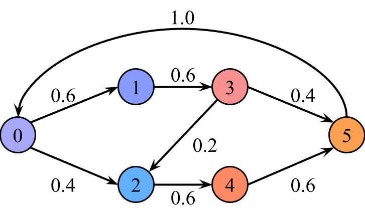
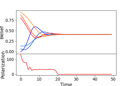
(a) Influence graph $\mathcal{I}$ and the corresponding evolution of beliefs and polarization for Example 3.2.

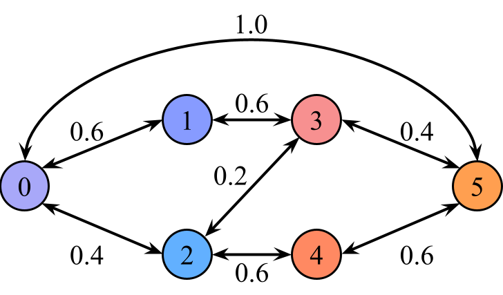
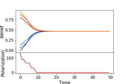
(b) Adding inverse influences to Figure 1(a).

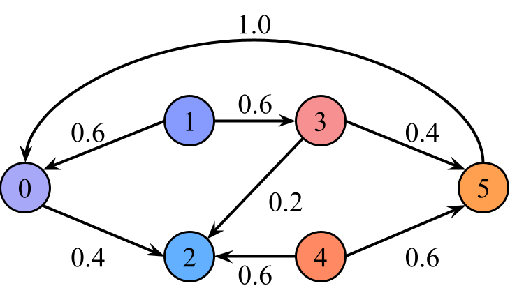
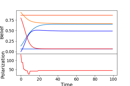
(c) Inversion of the influences $\mathcal{I}_{0,1}$ and $\mathcal{I}_{2,4}$ in Figure 1(a).

Figure 1. Influence graphs and the corresponding evolution of beliefs and polarization for Example 3.2. In each figure, the left-hand size is a graph representation of an influence graph, with nodes representing agents and each arrow from an agent $i$ to an agent $j$ labelled with the influence $\mathcal{I}_{i,j}$ the former carries on the latter. In each graph on the right-hand side, the $x$-axis represents the passage of time, and the $y$-axis is divided into: (i) an upper half depicting the evolution of beliefs for each agent at each time step (with each line representing the agent of same color in the corresponding influence graph); and (ii) a lower half depicting the corresponding measure of polarization of the network at each time step. In all cases the initial belief values for Agents $0$ to $5$ are, respectively, $0.0$, $0.0\overline{6}$, $0.1\overline{3}$, $0.8$, $0.8\overline{6}$, and $0.9\overline{3}$.

Now consider the influence graph in Figure 1(b), which is similar to Figure 1(a), but with reciprocal influences (i.e., the influence of $i$ over $j$ is the same as the influence of $j$ over $i$). Now Agents 1 and 2 do have direct influences over Agent 0, so the evolution of Agent $0$’s belief will be partly shaped by initially opposed agents: Agent 5 and the anti-vaxxers. But since Agent $0$’s opinion is very close to that of Agents 1 and 2, the confirmation-bias factor will help in keeping Agent $0$’s opinion close to their opinion against $p$. In particular, in contrast to the situation in Figure 1(a), Agent $0$ never becomes in favour of $p$. The evolution of the agents’ opinions and their polarization is shown in Figure 1(b). Notice that polarization vanishes around time 8 as the agents reach consensus, but this time they are more positive about (less against) $p$ than in the first situation.

Finally, consider the situation in Figure 1(c) obtained from Figure 1(a) by inverting the influences of Agent 0 over Agent 1 and Agent 2 over Agent 4. Notice that Agents 1 and 4 are no longer influenced by anyone though they influence others. Thus, as shown in Figure 1(c), their beliefs do not change over time, which means that the group does not reach consensus and polarization never disappears though it is considerably reduced. $\lhd$ The above example illustrates complex non-monotonic, overlapping, convergent, and non-convergent evolution of agent beliefs and polarization even in a small case with $n=6$ agents. Next we shall consider richer simulations on a greater variety of scenarios. These are instrumental in providing insight for theoretical results to be proven in the following sections.

3.3. Simulations

Here we present simulations for several influence graph topologies with $n=1,000$ agents (unless stated otherwise), which illustrate more complex behavior emerging from confirmation-bias interaction among agents. Our theoretical results in the next sections bring insight into the evolution of beliefs and polarization depending on graph topologies.

Next we provide the contexts used in our simulations.

Initial belief configurations

We consider the following initial belief configurations, depicted in Figure 2:

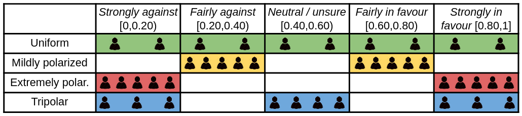
Figure 2. Depiction of the general shape of initial belief configurations (formally defined in Section 3.3), recreated here for a small group of only $n=10$ agents for exemplification purposes (since in the simulations the number of agents used is much larger). Each row represents an initial belief configuration, and the 10 agents’ opinions are distributed into columns according to their level of belief in the veracity of the proposition of interest. Empty cells represent positions that are not held by any agent, whereas the other cells have agents with beliefs uniformly distributed in the corresponding range (as formally defined in Section 3.3). Colors are used only to facilitate the visualization of each configuration.

• A uniform belief configuration representing a set of agents whose beliefs are as varied as possible, all equally spaced in the interval $[0,1]$: for every $i$,

  $$B^{0}_{i}=\nicefrac{{i}}{{(n{-}1)}}.$$

• A mildly polarized belief configuration with agents evenly split into two groups with moderately dissimilar inter-group beliefs compared to intra-group beliefs: for every $i$,

  $$B^{0}_{i}=\begin{cases}\nicefrac{{0.2i}}{{\lceil\nicefrac{{n}}{{2}}\rceil}}+0.2,&\text{if $i<\lceil\nicefrac{{n}}{{2}}\rceil$,}\\ \nicefrac{{0.2(i{-}\lceil\nicefrac{{n}}{{2}}\rceil)}}{{(n{-}\lceil\nicefrac{{n}}{{2}}\rceil)}}+0.6&\text{otherwise.}\end{cases}$$

• An extremely polarized belief configuration representing a situation in which half of the agents strongly believe the proposition, whereas half strongly disbelieve it: for every $i$,

  $$B^{0}_{i}=\begin{cases}\nicefrac{{0.2i}}{{\lceil\nicefrac{{n}}{{2}}\rceil}},&\text{if $i<\lceil\nicefrac{{n}}{{2}}\rceil$,}\\ \nicefrac{{0.2(i{-}\lceil\nicefrac{{n}}{{2}}\rceil)}}{{(n{-}\lceil\nicefrac{{n}}{{2}}\rceil)}}+0.8,&\text{otherwise.}\end{cases}$$

• A tripolar configuration with agents divided into three groups: for every $i$,

  $$B^{0}_{i}=\begin{cases}\nicefrac{{0.2i}}{{\lfloor\nicefrac{{n}}{{3}}\rfloor}},&\text{if $i<\lfloor{\nicefrac{{n}}{{3}}}\rfloor$,}\\ \nicefrac{{0.2(i{-}\lfloor{\nicefrac{{n}}{{3}}}\rfloor)}}{{(\lceil\nicefrac{{2n}}{{3}}\rceil{-}\lfloor{\nicefrac{{n}}{{3}}}\rfloor)}}+0.4,&\text{if $\lfloor{\nicefrac{{n}}{{3}}}\rfloor\leq i<\lceil\nicefrac{{2n}}{{3}}\rceil$,}\\ \nicefrac{{0.2(i{-}\lceil\nicefrac{{2n}}{{3}}\rceil)}}{{(n{-}\lceil\nicefrac{{2n}}{{3}}\rceil)}}+0.8,&\text{otherwise.}\end{cases}$$

Influence graphs

As for influence graphs, we consider the following ones, depicted in Figure 3:

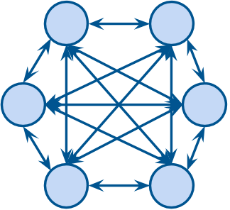
(a) $C$-clique.

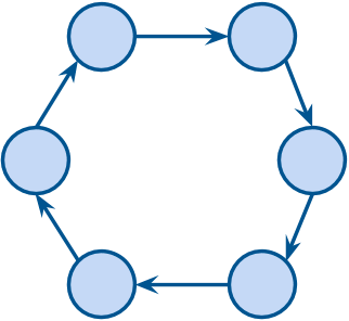
(b) Circular.

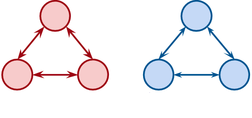
(c) Disconnected groups.

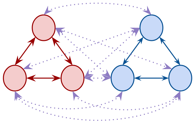
(d) Faintly communicating groups.

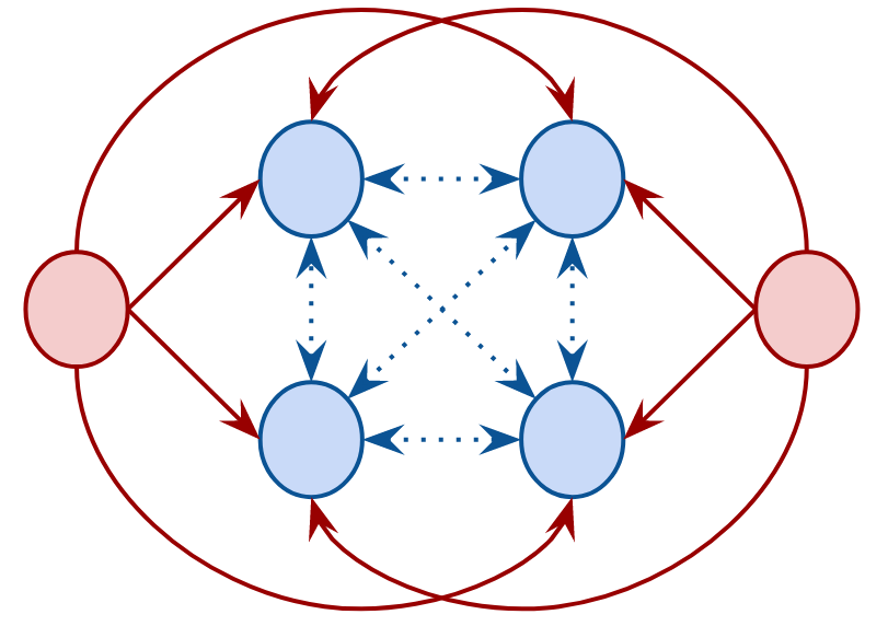
(e) Unrelenting influencers.

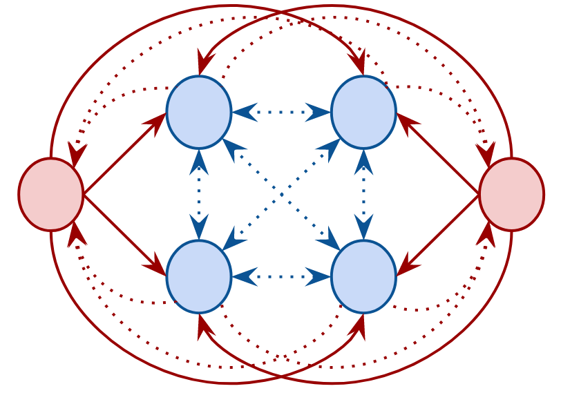
(f) Malleable influencers.

Figure 3. Depiction of the general shape of influence graphs (formally defined in Section 3.3), recreated here for a small group of only $n=6$ agents for exemplification purposes (since in the simulations the number of agents used is much larger). Solid (respectively, dashed) arrows indicate that the originating agent has relatively high (respectively, low) influence on the receiving agent. In influence graphs in which agents can be divided into groups with different behaviors, colors are used to indicate such groups.

• A $C$-clique influence graph $\mathcal{I}^{\textit{clique}}$, in which each agent influences every other with constant value $C=0.5$: for every $i,j$ such that $i{\neq}j$,

  $$\mathcal{I}^{\textit{clique}}_{i,j}=0.5~{}.$$

  This represents the particular case of a social network in which all agents interact among themselves, and are all immune to authority bias.

• A circular influence graph $\mathcal{I}^{\textit{circ}}$ representing a social network in which agents can be organized in a circle in such a way each agent is only influenced by its predecessor and only influences its successor: for every $i,j$ such that $i{\neq}j$,

  $$\mathcal{I}^{\textit{circ}}_{i,j}=\begin{cases}0.5,&\text{if (i{+}1)\,\text{mod}\,n = j,}\\ 0,&\text{otherwise.}\end{cases}$$

  This is a simple instance of a balanced graph (in which each agent’s influence on others is as high as the influence received, as in Definition 5.1 ahead), which is a pattern commonly encountered in some sub-networks.

• A disconnected influence graph $\mathcal{I}^{\textit{disc}}$ representing a social network sharply divided into two groups in such a way that agents within the same group can considerably influence each other, but not at all agents in the other group: for every $i,j$ such that $i{\neq}j$,

  $$\mathcal{I}^{\textit{disc}}_{i,j}=\begin{cases}0.5,&\text{if $i,j$ are both ${<}\lceil\nicefrac{{n}}{{2}}\rceil$ or both ${\geq}\lceil\nicefrac{{n}}{{2}}\rceil$,}\\ 0,&\text{otherwise.}\end{cases}$$

• A faintly communicating influence graph $\mathcal{I}^{\textit{faint}}$ representing a social network divided into two groups that evolve mostly separately, with only faint communication between them. More precisely, agents from within the same group influence each other much more strongly than agents from different groups: for every $i,j$ such that $i{\neq}j$,

  $$\mathcal{I}^{\textit{faint}}_{i,j}=\begin{cases}0.5,&\text{if $i,j$ are both ${<}\lceil\nicefrac{{n}}{{2}}\rceil$ or both ${\geq}\lceil\nicefrac{{n}}{{2}}\rceil$,}\\ 0.1,&\text{otherwise.}\end{cases}$$

  This could represent a small, ordinary social network, where some close groups of agents have strong influence on one another, and all agents communicate to some extent.

• An unrelenting influencers influence graph $\mathcal{I}^{\textit{unrel}}$ representing a scenario in which two agents (say, $0$ and $n{-}1$) exert significantly stronger influence on every other agent than these other agents have among themselves: for every $i,j$ such that $i{\neq}j$,

  $$\mathcal{I}^{\textit{unrel}}_{i,j}=\begin{cases}0.6,&\text{if $i=0$ and $j\neq n{-}1$ or $i=n{-}1$ and $j\neq 0$,}\\ 0,&\text{if $j=0$ or $j=n{-}1$,}\\ 0.1,&\text{if $0\neq i\neq n{-}{1}$ and $0\neq j\neq n{-}{1}$.}\end{cases}$$

  This could represent, e.g., a social network in which two totalitarian media companies dominate the news market, both with similarly high levels of influence on all agents. The networks have clear agendas to push forward, and are not influenced in a meaningful way by other agents.

• A malleable influencers influence graph $\mathcal{I}^{\textit{malleable}}$ representing a social network in which two agents have strong influence on every other agent, but are barely influenced by anyone else: for every $i,j$ such that $i{\neq}j$,

  $$\mathcal{I}^{\textit{malleable}}_{i,j}=\begin{cases}0.8,&\text{if $i=0$ and $j\neq n{-}1$,}\\ 0.4,&\text{if $i=n{-}1$ and $j\neq 0$,}\\ 0.1,&\text{if $j=0$ or $j=n{-}1$,}\\ 0.1,&\text{if $0\neq i\neq n{-}{1}$ and $0\neq j\neq n{-}{1}$.}\end{cases}$$

  This scenario could represent a situation similar to the “unrelenting influencers” scenario above, with two differences. First, one TV network has much higher influence than the other. Second, the networks are slightly influenced by all the agents (e.g., by checking ratings and choosing what news to cover accordingly).

We simulated the evolution of agents’ beliefs and the corresponding polarization of the network for all combinations of initial belief configurations and influence graphs presented above, using both the confirmation-bias update-function (Definition 2.2) and the classical update-function (Remark 2). Simulations of circular influences used $n=12$ agents, whereas the rest used $n=1,000$ agents. Both the Python implementation of the model and the Jupyter Notebook containing the simulations are available on GitHub [AAK⁺21].

The cases in which agents employ the confirmation-bias update-function, which is the core of the present work, are summarized in Figure 4. In that figure, each column corresponds to a different initial belief configuration, and each row corresponds to a different influence graph, so we can visualize how the behavior of polarization under confirmation bias changes when we fix an influence graph (row) and vary the initial belief configuration (column), or vice-versa. In Section 4 and Section 5 we shall discuss some of these results in more detail when illustrating our formal results. But first, in the following section we highlight some insights on the evolution of polarization we obtain from the whole set of simulations.

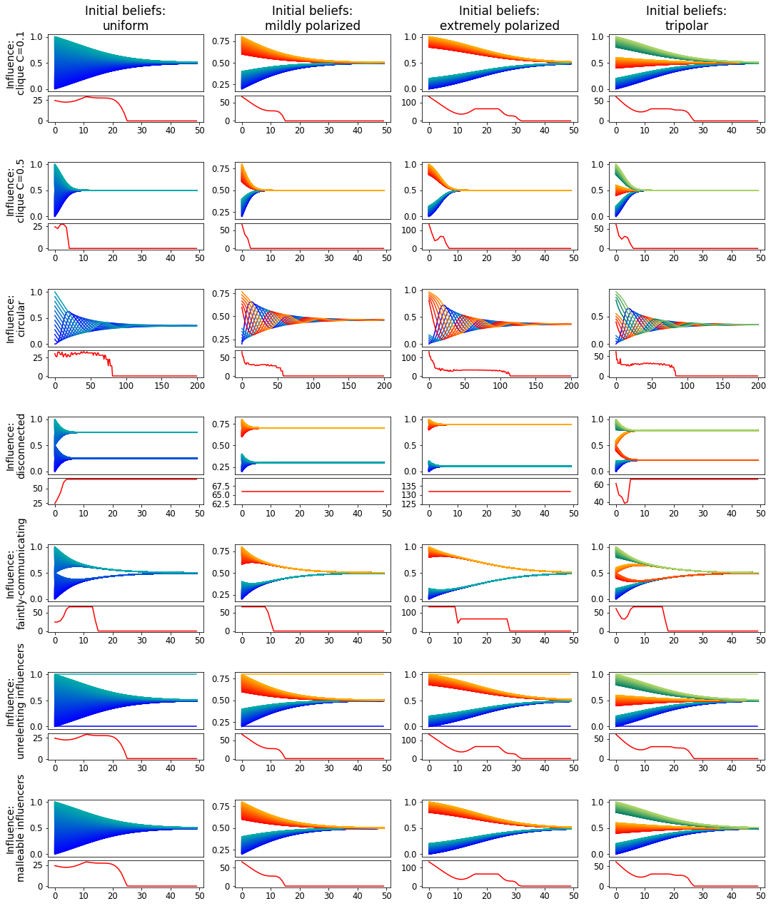
Figure 4. Evolution of belief and polarization under confirmation-bias. Each row (resp. column) contains all graphs with the same influence graph (resp. initial belief configuration). Circular influences used $n=12$ agents, the rest used $n=1,000$ agents. Each graph should be read as in Figure 1. Agents with similar behavior are grouped by colors: e.g., in all graphs in the rightmost column (tripolar initial belief configuration) all agents initiating in one of the three poles have the same color (green, orange, or blue).

3.4. Insights from simulations

We divide our discussion into “expected” and “unexpected” behaviors identified.

3.4.1. Analysis of “expected” behavior of polarization.

We start by considering the cases in which our simulations agree with some perhaps “expected” behavior of polarization. For this task, we focus on a scenario in which agents start off with varied opinions, represented by the uniform initial belief configuration, and all interact with each other via a $C$-clique influence graph. We consider both the cases in which agents incorporate new information in a classic way without confirmation bias (Remark 2), and in which agents present confirmation bias (Definition 2.2). These “expected” results are shown in Figure 5.

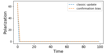
(a) Comparison of update functions under the mildly polarized initial belief configuration, and the $C$-clique influence graph.

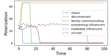
(b) Comparison of influence graphs under the confirmation-bias update function, and the uniform initial belief configuration.

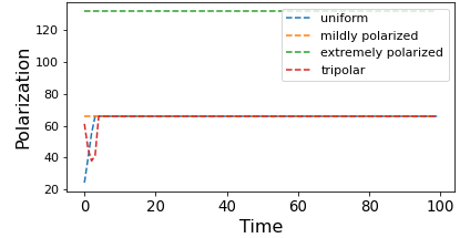
(c) Comparison of initial belief configurations under the $C$-clique influence graph, and the classical update.

Figure 5. Examples of “expected” behavior of the evolution of polarization.

In particular, Figure 5(a) meets our expectation that social networks in which all agents can interact in a direct way eventually converge to a consensus (i.e., polarization disappears), even if agents start off with very different opinions and are prone to confirmation bias. Figure 5(b) shows that for the same fixed update function and initial belief configuration, different interaction graphs may lead to very different evolutions of polarization: it grows to a maximum if agents are disconnected, achieves a very low yet non-zero value in the presence of 2 unrelenting influencers, and disappears in all other cases (i.e., when agents can influence each other, even if indirectly). Finally, Figure 5(c) shows that when there are agents that do not communicate with each other at all, as in a disconnected influence graph, then even rational agents updating beliefs according to the classic update function may not reach consensus, and polarization may stabilize at relatively high values.

We notice that some of the expected behaviors described in this section will follow from the results of in Section 5 (see, e.g., Theorem 16).

3.4.2. Analysis of perhaps “unexpected” behavior of polarization.

We now turn our attention interesting cases in which the simulations help shed light on perhaps counter-intuitive behavior of the dynamics of polarization. In the following we organize these insights into several topics.

Polarization is not necessarily a monotonic function of time.

At first glance it may seem that for a fixed social network configuration, polarization either only increases or decreases with time. Perhaps surprisingly, this is not so, as illustrated in Figure 6.

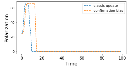
(a) Comparison of update functions under the uniform initial belief configuration, and the faintly communicating influence graph.

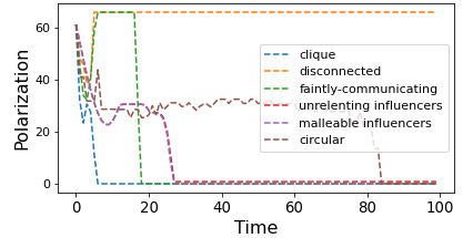
(b) Comparison of interaction graphs under the confirmation-bias update, and the midly polarized initial belief configuration.

Figure 6. Examples of cases in which the evolution of polarization is not monotonic.

We start by noticing that Figure 6(a) shows that for a uniform initial belief configuration and an interaction graph with two faintly communicating groups, no matter the update function, polarization increases before decreasing again and stabilizing at a lower level. This is explained by the fact that in such a set-up agents within the same group will reach consensus relatively fast, which will lead society to two clear poles and increase polarization at an initial stage. However, as the two groups continue to communicate over time, even if faintly, a general consensus is eventually achieved.

Figure 6(b) shows that a tripolar social network in which agents have confirmation bias, a similar phenomenon occurs for all interaction graphs. The only exceptions are the cases of disconnected groups, in which polarization stabilizes at a high level, and of unrelenting influencers, in which polarization stabilizes at a very low yet non-zero level. In the first case, this happens because the disconnected groups reach internal consensus but remain far from the other group, since they do not communicate. This represents a high level of polarization. The case of two unrelenting influencers retains a low level of polarization simply because the opinions of the unrelenting influencers never change, even if the rest of agents attain consensus. Another interesting case is that of two faintly communicating groups: here polarization first increases as the groups reach internal consensus, but then the two groups move toward one another and polarization decreases. The other two interaction graphs also stabilize to zero polarization.

The effect of different update functions.

Figure 7 shows a comparison of different update functions in various interesting scenarios.

(a) Comparison of update functions under the uniform initial belief configuration, and the disconnected influence graph.

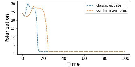
(b) Comparison of update functions under the uniform belief configuration and the unrelenting-influencers influence graph.

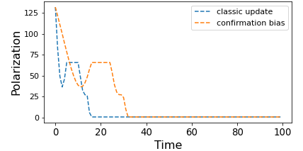
(c) Comparison of update functions under the extremely-polarized initial belief configuration, and the unrelenting-influencers influence graph.

Figure 7. Comparison of different update functions.

In particular, Figure 7(a) shows that, as expected, polarization can permanently increase in a disconnected social network, with little difference between the behavior of different update functions. Figure 7(b) depicts the effects of the two different update functions beginning from a uniform belief configuration, with two unrelenting influencers as the influence function. In both cases, all agents except the influencers eventually reach a belief value of 0.5 (the middle of the belief spectrum, between the two extreme agents), representing an increased but still fairly low level of polarization. The classic belief update function achieves this equilibrium fastest, since in under confirmation bias agents are less influenced by others whose beliefs are far from their own, so their beliefs change more slowly. Finally, Figure 7(c) shows that even under two extreme unrelenting influencers, consensus is eventually nearly reached, since everyone except the influencers eventually reaches a belief configuration between the beliefs of the two influencers.

The effect of different interaction graphs.

Figure 8 shows a comparison of different interaction graphs in various scenarios.

(a) Comparison of interaction graphs under the confirmation-bias update, and the uniform initial belief configuration.

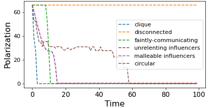
(b) Comparison of interaction graphs under the confirmation-bias update, and the mildly polarized initial belief configuration.

Figure 8. Comparison of different interaction graphs.

Figures 8(a) and 8(b) show that a faintly communicating graph leads to a temporary peak in polarization, which is reversed in all cases. As we discussed, this is explained by the fact that agents within the same group achieve consensus faster than agents in different groups, leading to a temporary increase in polarization. Note as well that both figures show that the presence of two unrelenting influencers pushing their agendas is sufficient prevent consensus-reaching, even if polarization remains at a very low level.

The effect of different initial belief configurations.

Figure 9 compares different belief configurations in various scenarios.

(a) Comparison of initial belief configurations under the disconnected influence graph, and the classical update.

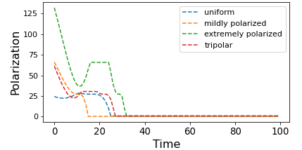
(b) Comparison of initial belief configurations under the unrelentin-influencers influence graph, and the confirmation-bias update.

Figure 9. Comparison of different initial belief configurations.

Figure 9(a) and Figure 9(b) show that even initial configurations with very different levels of polarization can converge to a same polarization level under both classic update and confirmation bias. However, not all initial belief configurations converge to a same final value, as is the case with the extremely polarized curve in Figure 9(a).

4. Belief and Polarization Convergence

Polarization tends to diminish as agents approximate a consensus, i.e., as they (asymptotically) agree upon a common belief value for the proposition of interest. Here and in Section 5 we consider meaningful families of influence graphs that guarantee consensus under confirmation bias. We also identify fundamental properties of agents, and the value of convergence. Importantly, we relate influence with the notion of flow in flow networks, and use it to identify necessary conditions for polarization not converging to zero.

4.1. Polarization at the limit

Proposition 1 states that our polarization measure on a belief configuration (Definition 2.1) is zero exactly when all belief values in it lie within the same bin of the underlying discretization $D_{k}=I_{0}\ldots I_{k-1}$ of $[0,1]$. In our model polarization converges to zero if all agents’ beliefs converge to a same non-borderline value. More precisely:

Lemma 4 (Zero Limit Polarization).

Let $v$ be a non-borderline point of $D_{k}$ such that for every $i\in\mathcal{A}$, $\lim_{t\allowbreak\mathrel{\mathop{\hbox to8.4pt{\rightarrowfill}}\limits}\infty}B^{t}_{i}=v$. Then $\lim_{t\allowbreak\mathrel{\mathop{\hbox to8.4pt{\rightarrowfill}}\limits}\infty}\rho(B^{t})=0$.

To see why we exclude the $k-1$ borderline values of $D_{k}$ in the above lemma, assume $v\in I_{m}$ where $m\in\{0,\ldots,k-1\}$ is a borderline value. Suppose that there are two agents $i$ and $j$ whose beliefs converge to $v$, but with the belief of $i$ staying always within $I_{m}$ whereas the belief of $j$ remains outside of $I_{m}$. Under these conditions one can verify, using Definition 2.1 and Definition 2.1, that $\rho$ will not converge to $0$. This situation is illustrated in Figure 10(b) assuming a discretization $D_{2}=[0,\nicefrac{{1}}{{2}}),[\nicefrac{{1}}{{2}},1]$ whose only borderline is $\nicefrac{{1}}{{2}}$. Agents’ beliefs converge to value $v=\nicefrac{{1}}{{2}}$, but polarization does not converge to 0. In contrast, Figure 10(c) illustrates Lemma 4 for $D_{3}=[0,\nicefrac{{1}}{{3}}),[\nicefrac{{1}}{{3}},\nicefrac{{2}}{{3}}),[\nicefrac{{2}}{{3}},1]$.  

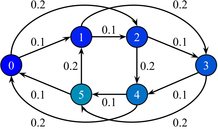
(a) Influence graph.

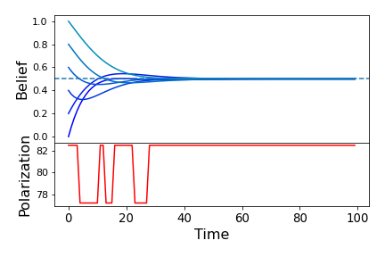
(b) Evolution of beliefs and polarization, 2 bins.

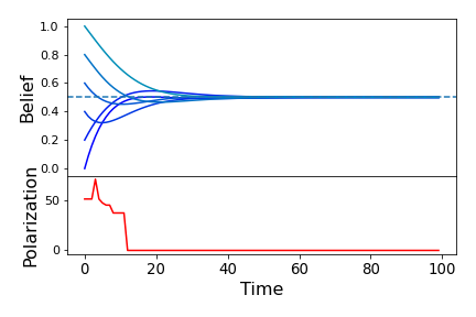
(c) Evolution of beliefs and polarization, 3 bins.

Figure 10. Belief convergence to borderline value $0.5$. Polarization does not converge to 0 with equal-length 2 bins (Figure 10(b)) but it does with 3 equal-length bins (Figure 10(c)). In all cases the initial belief values for Agents $0$ to $5$ are, respectively, $0.0$, $0.2$, $0.4$, $0.6$, $0.8$, and $1.0$ and the influence graph is the one depicted in Figure 10(a). The graphs for the evolution of belief and polarization should be read as in Figure 1.

4.2. Convergence under Confirmation Bias in Strongly Connected Influence

We now introduce the family of strongly-connected influence graphs, which includes cliques, that describes scenarios where each agent has an influence over all others. Such influence is not necessarily direct in the sense defined next, or the same for all agents, as in the more specific cases of cliques.

[Influence Paths] Let $C\in(0,1]$. We say that $i$ has a direct influence $C$ over $j$, written $i{\stackrel{{\scriptstyle\,\,C\,\,}}{{\rightarrow}}}j$, if $\mathcal{I}_{i,j}=C$.

An influence path is a finite sequence of distinct agents from $\mathcal{A}$ where each agent in the sequence has a direct influence over the next one. Let $p$ be an influence path $i_{0}i_{1}\ldots i_{n}$. The size of $p$ is $|p|=n$. We also use $i_{0}{\stackrel{{\scriptstyle\,\,C_{1}\,\,}}{{\rightarrow}}}i_{1}{\stackrel{{\scriptstyle\,\,C_{2}\,\,}}{{\rightarrow}}}\ldots{\stackrel{{\scriptstyle\,\,C_{n}\,\,}}{{\rightarrow}}}i_{n}$ to denote $p$ with the direct influences along this path. We write $i_{0}\stackrel{{\scriptstyle\,\,C\,\,}}{{\leadsto_{p}}}i_{n}$ to indicate that the product influence of $i_{0}$ over $i_{n}$ along $p$ is $C=C_{1}\times\cdots\times C_{n}$.

We often omit influence or path indices from the above arrow notations when they are unimportant or clear from the context. We say that $i$ has an influence over $j$ if $i{\stackrel{{\scriptstyle\,\,\,\,}}{{\leadsto}}}j$.

The next definition is akin to the graph-theoretical notion of strong connectivity. [Strongly Connected Influence] We say that an influence graph $\mathcal{I}$ is strongly connected if for all $i$, $j\in\mathcal{A}$ such that $i{\neq}j$, $i{\stackrel{{\scriptstyle\,\,\,\,}}{{\leadsto}}}j$.

Remark 5.

For technical reasons we assume that, initially, there are no two agents $i,j\in\mathcal{A}$ such that $B^{0}_{i}=0$ and $B^{0}_{j}=1$. This implies that for every $i,j\in\mathcal{A}$: $\beta^{0}_{i,j}>0$ where $\beta^{0}_{i,j}$ is the confirmation bias of $i$ towards $j$ at time $0$ (See Definition 2.2). Nevertheless, at the end of this section we will address the cases in which this condition does not hold.

We shall use the following notation for the extreme beliefs of agents.

[Extreme Beliefs] Define $max^{t}=\max_{i\in\mathcal{A}}B^{t}_{i}$ and $min^{t}=\max_{i\in\mathcal{A}}B^{t}_{i}$ as the functions giving the maximum and minimum belief values, respectively, at time $t$.

It is worth noticing that extreme agents –i.e., those holding extreme beliefs– do not necessarily remain the same across time steps. Figure 1(a) illustrates this point: Agent 0 goes from being the one most against the proposition of interest at time $t=0$ to being the one most in favour of it around $t=8$. Also, the third row of Figure 4 shows simulations for a circular graph under several initial belief configurations. Note that under all initial belief configurations different agents alternate as maximal and minimal belief holders.

Nevertheless, in what follows will show that the beliefs of all agents, under strongly-connected influence and confirmation bias, converge to the same value since the difference between $min^{t}$ and $max^{t}$ goes to 0 as $t$ approaches infinity. We begin with a lemma stating a property of the confirmation-bias update: The belief value of any agent at any time is bounded by those from extreme agents in the previous time unit.

Lemma 6 (Belief Extremal Bounds).

For every $i\in\mathcal{A}$, $min^{t}\leq B^{t+1}_{i}\leq max^{t}$.

The next corollary follows from the assumption in Remark 5 and Lemma 6.

Corollary 7.

For every $i,j\in\mathcal{A}$, $t\geq 0$: $\beta^{t}_{i,j}>0$.

Note that monotonicity does not necessarily hold for belief evolution. This is illustrated by Agent 0’s behavior in Figure 1(a). However, it follows immediately from Lemma 6 that $min$ and $max$ in Definition 5 are monotonically non-decreasing and non-increasing functions of $t$.

Corollary 8 (Monotonicity of Extreme Beliefs).

$max^{t+1}\leq max^{t}$ and $min^{t+1}\geq min^{t}$ for all $t\in{\rm Nature}$.

Monotonicity and the bounding of $max^{\cdot}$, $min^{\cdot}$ within $[0,1]$ lead us, via the Monotonic Convergence Theorem [Soh14], to the existence of limits for beliefs of extreme agents.

Theorem 9 (Limits of Extreme Beliefs).

There are $U,L\in[0,1]$ such that $\lim_{t\allowbreak\mathrel{\mathop{\hbox to8.4pt{\rightarrowfill}}\limits}\infty}max^{t}=U$ and $\lim_{t\allowbreak\mathrel{\mathop{\hbox to8.4pt{\rightarrowfill}}\limits}\infty}min^{t}=L$.

We still need to show that $U$ and $L$ are the same value. For this we prove a distinctive property of agents under strongly connected influence graphs: the belief of any agent at time $t$ will influence every other agent by the time $t+|\mathcal{A}|-1$. This is precisely formalized below in Lemma 11. First, however, we introduce some bounds for confirmation-bias and influence, as well as notation for the limits in Theorem 9.

[Min Factors] Define $\beta_{min}=\min_{i,j\in\mathcal{A}}\beta^{0}_{i,j}$ as the minimal confirmation bias factor at $t=0$. Also let $\mathcal{I}_{min}$ be the smallest positive influence in $\mathcal{I}$. Furthermore, let $L=\lim_{t\allowbreak\mathrel{\mathop{\hbox to8.4pt{\rightarrowfill}}\limits}\infty}min^{t}$ and $U=\lim_{t\allowbreak\mathrel{\mathop{\hbox to8.4pt{\rightarrowfill}}\limits}\infty}max^{t}$.

Notice that since $min^{t}$ and $max^{t}$ do not get further apart as the time $t$ increases (Corollary 8), $\min_{i,j\in\mathcal{A}}\beta^{t}_{i,j}$ is a non-decreasing function of $t$. Therefore $\beta_{min}$ acts as a lower bound for the confirmation-bias factor in every time step.

Proposition 10.

$\beta_{min}=\min_{i,j\in\mathcal{A}}\beta^{t}_{i,j}$ for every $t>0$.

We use the factor $\beta_{min}$ in the next result to establish that the belief of agent $i$ at time $t$, the minimum confirmation-bias factor, and the maximum belief at $t$ act as bound of the belief of $j$ at $t+|p|$, where $p$ is an influence path from $i$ and $j$.

Lemma 11 (Path bound).

If $\mathcal{I}$ is strongly connected:

1. Let $p$ be an arbitrary path $i\stackrel{{\scriptstyle\,\,C\,\,}}{{\leadsto_{p}}}j$. Then

   $$B^{t+|p|}_{j}\leq max^{t}+\nicefrac{{C\beta_{min}^{|p|}}}{{|\mathcal{A}|^{|p|}}}(B^{t}_{i}-max^{t}).$$

2. Let $\mathtt{m}^{t}\in\mathcal{A}$ be an agent holding the least belief value at time $t$ and $p$ be a path such that $\mathtt{m}^{t}\stackrel{{\scriptstyle\,\,\,\,}}{{\leadsto_{p}}}i$. Then

   $$B^{t+|p|}_{i}\leq max^{t}-\delta,$$

   with $\delta=\left(\nicefrac{{\mathcal{I}_{min}\beta_{min}}}{{|\mathcal{A}|}}\right)^{|p|}(U-L)$.

Next we establish that all beliefs at time $t+|\mathcal{A}|-1$ are smaller than the maximal belief at $t$ by a factor of at least $\epsilon$ depending on the minimal confirmation bias, minimal influence and the limit values $L$ and $U$.

Lemma 12.

Suppose that $\mathcal{I}$ is strongly-connected.

1. If $B^{t+n}_{i}\leq max^{t}-\gamma$ and $\gamma\geq 0$ then $B^{t+n+1}_{i}\leq max^{t}-\nicefrac{{\gamma}}{{|\mathcal{A}|}}$.

2. $B^{t+|\mathcal{A}|-1}_{i}\leq max^{t}-\epsilon$, where $\epsilon$ is equal to $\left(\nicefrac{{\mathcal{I}_{min}\beta_{min}}}{{|\mathcal{A}|}}\right)^{|\mathcal{A}|-1}(U-L)$.

Lemma 12(2) states that $\max^{\cdot}$ decreases by at least $\epsilon$ after $|A|-1$ steps. Therefore, after $m(|A|-1)$ steps it should decrease by at least $m\epsilon$.

Corollary 13.

If $\mathcal{I}$ is strongly connected, $max^{t+m(|\mathcal{A}|-1)}\leq max^{t}-m\epsilon$ for $\epsilon$ in Lemma 12.

We can now state that in strongly connected influence graphs extreme beliefs eventually converge to the same value. The proof uses Corollary 7 and Corollary 13 above.

Theorem 14.

If $\mathcal{I}$ is strongly connected then $\lim_{t\allowbreak\mathrel{\mathop{\hbox to8.4pt{\rightarrowfill}}\limits}\infty}max^{t}=\lim_{t\allowbreak\mathrel{\mathop{\hbox to8.4pt{\rightarrowfill}}\limits}\infty}min^{t}$.

Combining Theorem 14, the assumption in Remark 5 and the Squeeze Theorem [Soh14], we conclude that for strongly-connected graphs, all agents’ beliefs converge to the same value.

Corollary 15.

If $\mathcal{I}$ is strongly connected then for all $i,j\in\mathcal{A},\lim_{t\allowbreak\mathrel{\mathop{\hbox to8.4pt{\rightarrowfill}}\limits}\infty}B^{t}_{i}=\lim_{t\allowbreak\mathrel{\mathop{\hbox to8.4pt{\rightarrowfill}}\limits}\infty}B^{t}_{j}$.

4.2.1. The Extreme Cases.

We assumed in Remark 5 that there were no two agents $i,j$ such that $B^{t}_{i}=0$ and $B^{t}_{j}=1$. Theorem 16 below addresses the situation in which this does not happen. More precisely, it establishes that under confirmation-bias update, in any strongly-connected, non-radical society, agents’ beliefs eventually converge to the same value.

[Radical Beliefs] An agent $i\in\mathcal{A}$ is called radical if $B_{i}=0$ or $B_{i}=1$. A belief configuration $B$ is radical if every $i\in\mathcal{A}$ is radical.

Theorem 16 (Confirmation-Bias Belief Convergence).

In a strongly connected influence graph and under the confirmation-bias update-function, if $B^{0}$ is not radical then for all $i,j\in\mathcal{A}$, $\lim_{t\allowbreak\mathrel{\mathop{\hbox to8.4pt{\rightarrowfill}}\limits}\infty}B^{t}_{i}=\lim_{t\allowbreak\mathrel{\mathop{\hbox to8.4pt{\rightarrowfill}}\limits}\infty}B^{t}_{j}$. Otherwise for every $i\in\mathcal{A}$, $B^{t}_{i}=B^{t+1}_{i}\in\{0,1\}$.

We conclude this section by emphasizing that belief convergence is not guaranteed in non strongly-connected graphs. Figure 1(c) from the vaccine example shows such a graph where neither belief convergence nor zero-polarization is obtained.

5. Conditions for Polarization

We now use concepts from flow networks to identify insightful necessary conditions for polarization never disappearing. Understanding the conditions when polarization does not disappear under confirmation bias is one of the main contributions of this paper.

5.1. Balanced Influence: Circulations

The following notion is inspired by the circulation problem for directed graphs (or flow network) [Die17]. Given a graph $G=(V,E)$ and a function $c:E\allowbreak\mathrel{\mathop{\hbox to11.99998pt{\rightarrowfill}}\limits}\mathbb{R}$ (called capacity), the problem involves finding a function $f:E\allowbreak\mathrel{\mathop{\hbox to11.99998pt{\rightarrowfill}}\limits}\mathbb{R}$ (called flow) such that:

1. $f(e)\leq c(e)$ for each $e\in E$; and

2. $\sum_{(v,w)\in E}f(v,w)=\sum_{(w,v)\in E}f(w,v)$ for all $v\in V$.

Such an $f$ exists is called a circulation for $G$ and $c$.

Thinking of flow as influence, the second condition, called flow conservation, corresponds to requiring that each agent influences others as much as is influenced by them.

[Balanced Influence] We say that $\mathcal{I}$ is balanced (or a circulation) if every $i\in\mathcal{A}$ satisfies the constraint $\sum_{j\in\mathcal{A}}\mathcal{I}_{i,j}=\sum_{j\in\mathcal{A}}\mathcal{I}_{j,i}$.

Cliques and circular graphs, where all (non-self) influence values are equal, are balanced (see Figure 3(b)). The graph of our vaccine example (Figure 1) is a circulation that is neither a clique nor a circular graph. Clearly, influence graph $\mathcal{I}$ is balanced if it is a solution to a circulation problem for some $G=(\mathcal{A},\mathcal{A}\times\mathcal{A})$ with capacity $c:\mathcal{A}\times\mathcal{A}\allowbreak\mathrel{\mathop{\hbox to11.99998pt{\rightarrowfill}}\limits}[0,1]$.

Next we use a fundamental property from flow networks describing flow conservation for graph cuts [Die17]. Interpreted in our case it says that any group of agents $A{\subseteq}\mathcal{A}$ influences other groups as much as they influence $A$.

Proposition 17 (Group Influence Conservation).

Let $\mathcal{I}$ be balanced and $\{A,B\}$ be a partition of $\mathcal{A}$. Then

$$\sum_{i\in A}\sum_{j\in B}\mathcal{I}_{i,j}=\sum_{i\in A}\sum_{j\in B}\mathcal{I}_{j,i}.$$

We now define weakly connected influence. Recall that an undirected graph is connected if there is path between each pair of nodes.

[Weakly Connected Influence] Given an influence graph $\mathcal{I}$, define the undirected graph $G_{\mathcal{I}}=(\mathcal{A},E)$ where $\{i,j\}\in E$ if and only if $\mathcal{I}_{i,j}>0$ or $\mathcal{I}_{j,i}>0$. An influence graph $\mathcal{I}$ is called weakly connected if the undirected graph $G_{\mathcal{I}}$ is connected.

Weakly connected influence relaxes its strongly connected counterpart. However, every balanced, weakly connected influence is strongly connected as implied by the next lemma. Intuitively, circulation flows never leaves strongly connected components.

Lemma 18.

If $\mathcal{I}$ is balanced and $\mathcal{I}_{i,j}>0$ then $j{\stackrel{{\scriptstyle\,\,\,\,}}{{\leadsto}}}i$.

5.2. Conditions for Polarization

We have now all elements to identify conditions for permanent polarization. The convergence for strongly connected graphs (Theorem 16), the polarization at the limit lemma (Lemma 4), and Lemma 18 yield the following noteworthy result.

Theorem 19 (Conditions for Polarization).

Suppose that $\lim_{t\allowbreak\mathrel{\mathop{\hbox to8.4pt{\rightarrowfill}}\limits}\infty}\rho(B^{t}){\neq}0$. Then either:

1. $\mathcal{I}$ is not balanced;

2. $\mathcal{I}$ is not weakly connected;

3. $B^{0}$ is radical; or

4. for some borderline value $v$, $\lim_{t\allowbreak\mathrel{\mathop{\hbox to8.4pt{\rightarrowfill}}\limits}\infty}B^{t}_{i}=v$ for each $i\in\mathcal{A}$.

Hence, at least one of the four conditions is necessary for the persistence of polarization. If (1) then there must be at least one agent that influences more than what he is influenced (or vice versa). This is illustrated in Figure 1(c) from the vaccine example, where Agent 2 is such an agent. If (2) then there must be isolated subgroups of agents; e.g., two isolated strongly-connected components where the members of the same component will achieve consensus but the consensus values of the two components may be very different. This is illustrated in the fourth row of Figure 4. Condition (3) can be ruled out if there is an agent that is not radical, like in all of our examples and simulations. As already discussed, (4) depends on the underlying discretization $D_{k}$ (e.g., assuming equal-length bins if $v$ is borderline in $D_{k}$ it is not borderline in $D_{k+1}$, see Figure 10.).

5.3. Reciprocal and Regular Circulations

The notion of circulation allowed us to identify potential causes of polarization. In this section we will also use it to identify meaningful topologies whose symmetry can help us predict the exact belief value of convergence.

A reciprocal influence graph is a circulation where the influence of $i$ over $j$ is the same as that of $j$ over $i$, i.e, $\mathcal{I}_{i,j}=\mathcal{I}_{j,i}$. Also a graph is (in-degree) regular if the in-degree of each nodes is the same; i.e., for all $i,j\in\mathcal{A}$, $|\mathcal{A}_{i}|=|\mathcal{A}_{j}|$.

As examples of regular and reciprocal graphs, consider a graph $\mathcal{I}$ where all (non-self) influence values are equal. If $\mathcal{I}$ is circular then it is a regular circulation, and if $\mathcal{I}$ is a clique then it is a reciprocal regular circulation. Also we can modify slightly our vaccine example to obtain a regular reciprocal circulation as shown in Figure 11.

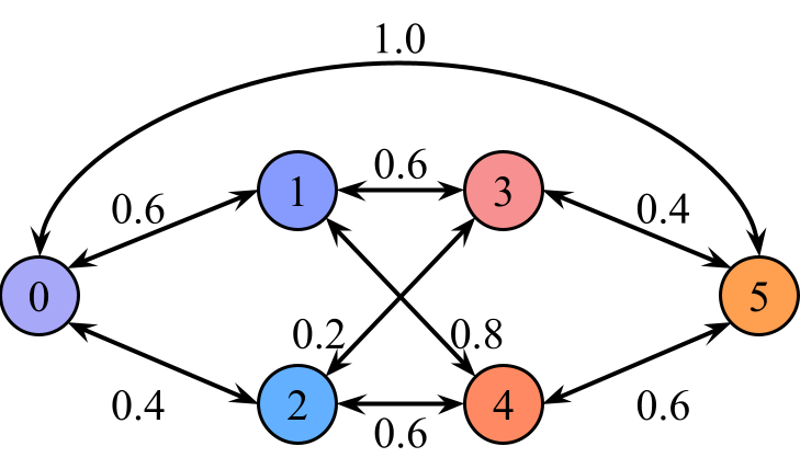
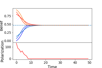
Figure 11. Regular and reciprocal influence, and the corresponding evolution of beliefs and polarization. This figure should be read as Figure 1.

The importance of regularity and reciprocity of influence graphs is that their symmetry is sufficient to the determine the exact value all the agents converge to under confirmation bias: the average of initial beliefs. Furthermore, under classical update (see Remark 2), we can drop reciprocity and obtain the same result. The result follows from Lemma 18, Theorem 16, Corollary 21, the Squeeze Theorem [Soh14] and by showing that $\sum_{i\in\mathcal{A}}B^{t}_{i}=\sum_{i\in\mathcal{A}}B^{t+1}_{i}$ using symmetries derived from reciprocity, regularity, and the fact that $\beta^{t}_{i,j}=\beta^{t}_{j,i}$.

Theorem 20 (Consensus Value).

Suppose that $\mathcal{I}$ is regular and weakly connected. If $\mathcal{I}$ is reciprocal and the belief update is confirmation-bias, or if the influence graph $\mathcal{I}$ is a circulation and the belief update is classical, then, for every $i\in\mathcal{A}$,

$$\lim_{t\allowbreak\mathrel{\mathop{\hbox to8.4pt{\rightarrowfill}}\limits}\infty}B^{t}_{i}=\frac{1}{|\mathcal{A}|}\sum_{j\in\mathcal{A}}B^{0}_{j}.$$

6. Related Work

6.1. Comparison to DeGroot’s model

DeGroot proposed a very influential model, closely related to our work, to reason about learning and consensus in multi-agent systems [DeG74], in which beliefs are updated by a constant stochastic matrix at each time step. More specifically, consider a group $\{1,2,\ldots,k\}$ of $k$ agents, such that each agent $i$ holds an initial (real-valued) opinion $F_{i}^{0}$ on a given proposition of interest. Let $T_{i,j}$ be a non-negative weight that agent $i$ gives to agent $j$’s opinion, such that $\sum_{j=1}^{k}T_{i,j}{=}1$. DeGroot’s model posits that an agent $i$’s opinion $F_{i}^{t}$ at any time $t{\geq}1$ is updated as $F_{i}^{t}{=}\sum_{j{=}1}^{k}T_{i,j}F_{i}^{t-1}$. Letting $F^{t}$ be a vector containing all agents’ opinions at time $t$, the overall update can be computed as $F^{t{+}1}{=}TF^{t}$, where $T{=}\{T_{i,j}\}$ is a stochastic matrix. This means that the $t$-th configuration (for $t{\geq}1$) is related to the initial one by $F^{t}{=}T^{t}F^{0}$, which is a property thoroughly used to derive results in the model.

When we use classical update (as in Remark 2), our model reduces to DeGroot’s via the transformation $F_{i}^{0}{=}B^{0}_{i}$, and $T_{i,j}{=}\nicefrac{{1}}{{|\mathcal{A}_{i}|}}\ \mathcal{I}_{j,i}$ if $i{\neq}j$, or $T_{i,j}{=}1{-}\nicefrac{{1}}{{|\mathcal{A}_{i}|}}\sum_{j{\in}\mathcal{A}_{i}}\mathcal{I}_{j,i}$ otherwise. Notice that $T_{i,j}{\leq}1$ for all $i$ and $j$, and, by construction, $\sum_{j{=}1}^{k}T_{i,j}{=}1$ for all $i$. The following result is an immediate consequence of this reduction.

Corollary 21.

In a strongly connected influence graph $\mathcal{I}_{,}$ and under the classical update function, for all $i,j{\in}\mathcal{A}$,

$$\lim_{t{\allowbreak\mathrel{\mathop{\hbox to8.4pt{\rightarrowfill}}\limits}}\infty}B^{t}_{i}=\lim_{t{\allowbreak\mathrel{\mathop{\hbox to8.4pt{\rightarrowfill}}\limits}}\infty}B^{t}_{j}.$$

Unlike its classical counterpart, however, the confirmation-bias update (Definition 2.2) does not have an immediate correspondence with DeGroot’s model. Indeed, this update is not linear due the confirmation-bias factor $\beta^{t}_{i,j}{=}1{-}|B^{t}_{j}{-}B^{t}_{i}|$. This means that in our model there is no immediate analogue of the relation among arbitrary configurations and the initial one as the relation in DeGroot’s model (i.e., $F^{t}{=}T^{t}F^{0}$). Therefore, proof techniques usually used in DeGroot’s model (e.g., based on Markov properties) are not immediately applicable to our model. In this sense our model is an extension of DeGroot’s, and we need to employ different proof techniques to obtain our results.

The Degroot-like models are also used in [GJ10]. Rather than examining polarization and opinions, this work is concerned with the network topology conditions under which agents with noisy data about an objective fact converge to an accurate consensus, close to the true state of the world. As already discussed the basic DeGroot model does not include confirmation bias, however [SSVL20, MBA20, MF15, HK02, CVCL20] all generalize DeGroot-like models to include functions that can be thought of as modelling confirmation bias in different ways, but with either no measure of polarization or a simpler measure than the one we use. [Mor05] discusses DeGroot models where the influences change over time, and [GS16] presents results about generalizations of these models, concerned more with consensus than with polarization.

6.2. Other related work

We summarize some other relevant approaches and put into perspective the novelty of our approach.

Polarization

Polarization was originally studied as a psychological phenomenon in [ML76], and was first rigorously and quantitatively defined by economists Esteban and Ray [ER94]. Their measure of polarization, discussed in Section 2, is influential, and we adopt it in this paper. Li et al. [LSSZ13], and later Proskurnikov et al. [PMC16] modeled consensus and polarization in social networks. Like much other work, they treat polarization simply as the lack of consensus and focus on when and under what conditions a population reaches an agreement. Elder’s work [Eld19] focuses on methods to avoid polarization, without using a quantitative definition of polarization.

Formal Models

Sîrbu et al. [SPGK18] use a model that updates probabilistically to investigate the effects of algorithmic bias on polarization by counting the number of opinion clusters, interpreting a single opinion cluster as consensus. Leskovec et al. [GG16] simulate social networks and observe group formation over time. Though belief update and group formation are related to our work [SPGK18, GG16] are not concerned with a measure for polarization.

Logic-based approaches

Liu et al. [LSG14] use ideas from doxastic and dynamic epistemic logics to qualitatively model influence and belief change in social networks. Seligman et al. [SLG11, SLG13] introduce a basic “Facebook logic.” This logic is non-quantitative, but its interesting point is that an agent’s possible worlds are different social networks. This is a promising approach to formal modeling of epistemic issues in social networks. Christoff [Chr16] extends facebook logic and develops several non-quantitative logics for social networks, concerned with problems related to polarization, such as information cascades. Young Pederson et al. [Ped, PSÅ19, PSÅ20] develop a logic of polarization, in terms of positive and negeative links between agents, rather than in terms of their quantitative beliefs. Baltag et al. [BCRS19] develop a dynamic epistemic logic of threshold models with imperfect information. In these models, agents either completely believe or completely disbelieve a proposition, and they update their belief over time based on the proportion of their neighbors that believe the proposition. Although this work is not concerned with polarization, it would be interesting to compare the situations where our model converges to the longterm outcomes of their threshold models, and consider the implications of the epistemic logic developed in their paper for our model. Hunter [Hun17] introduces a logic of belief updates over social networks where closer agents in the social network are more trusted and thus more influential. While beliefs in this logic are non-quantitative, there is a quantitative notion of influence between users.

Work on Users’ Influence

The seminal paper Huberman et al. [HRW08] is about determining which friends or followers in a user’s network have the most influence on the user. Although this paper does not quantify influence between users, it does address an important question to our project. Similarly, [DVZ03] focuses on finding most influential agents. This work on highly influential agents is relevant to our finding that such agents can maintain a network’s polarization over time.

Work on decentralized gossip protocols also examines the problem of information diffusion among agents from a different perspective [AGvdH15, AGvdH18, AvDGvdH14a, AvDGvdH14b]. The goal of a gossip protocol is for all the agents in a network to share all their information with as few communication steps as possible, using their own knowledge to choose their communication actions at each step. It may be possible to generalize results from gossip protocols in order to understand how quickly it is possible for a social network to reach consensus under certain conditions.

7. Conclusions and Future Work

In this paper we proposed a model for polarization and belief evolution for multi-agent systems under confirmation bias; a recurrent and systematic pattern of deviation from rationality when forming opinions in social networks and in society in general. We extended previous results in the literature by showing that also under confirmation bias, whenever all agents can directly or indirectly influence each other, their beliefs always converge, and so does polarization as long as the convergence value is not a borderline point. Nevertheless, we believe that our main contribution to the study of polarization is understanding how outcomes are structured when convergence does not obtain and polarization persists. Indeed, we have identified necessary conditions when polarization does not disappear, and the convergence values for some important network topologies.

As future work we plan to explore the following directions aimed at making the present model more robust.

7.1. Dynamic Influence

In the current work, we consider one agent’s influence on another to be static. For modelling short term belief change, this is a reasonable decision, but in order to model long term belief change in social networks over time, we need to include dynamic influence. In particular, agent $a$’s influence on agent $b$ should become stronger over time if agent $a$ sees $b$ as reliable, which means that $b$ mostly sends messages that are already close to the beliefs of agent $a$. Thus, we plan enrich our model with dynamic influence between agents: agent $a$’s influence on $b$ becomes stronger if $a$ communicates messages that $b$ agrees with, and it becomes weaker if $b$ mostly disagrees with the beliefs that are communicated by $a$. We expect that this change to the model will tend to increase group polarization, as agents who already tend to agree will have increasingly stronger influence on one another, and agents who disagree will influence one another less and less. This will be particularly useful for modelling filter bubbles [FGR16], and we will consult empirical work on this phenomenon in order to correctly include influence update in our model.

7.2. Multi-dimensional beliefs

The current paper considers the simple case where agents only have beliefs about one proposition. This simplification may be quite useful for modelling some realistic scenarios, such as beliefs along a liberal/conservative political spectrum, but we believe that it will not be sufficient for modelling all situations. To that end, we plan to develop models where agents have beliefs about multiple issues. This would allow us to represent, for example, Nolan’s two-dimensional spectrum of political beliefs, where individuals can be economically liberal or conservative, and socially liberal or conservative [BM68], since more nuanced belief situations such as this one cannot be modelled in a one-dimensional space. Since Esteban-Ray polarization considers individuals along a one-dimensional spectrum, we will extend Esteban-Ray polarization to more dimensions, or develop a new, multi-dimensional definition of polarization.

7.3. Sequential and asynchronous communication

In our current model, all agents communicate synchronously at every time step and update their beliefs accordingly. This simplification is a reasonable approximation of belief update for an initial study of group polarization, but in real social networks, communication may be both asynchronous and sequential, in the sense that messages are sent one by one between a pair of agents, rather than every agent sending every connected agent a message at every time step as in the current model. The current model is deterministic, but introducing sequential messages will add nondeterminism to the model, bringing new complications. We plan to develop a logic in the style of dynamic epistemic logic [Pla07] in order to reason about sequential messages. Besides being sequential, communication in real social networks is also asynchronous, making it particularly difficult to represent agents’ knowledge and beliefs about one another, as discussed in [KMS15, KMS19]. Eventually, we plan to include asynchronous communication and its effects on beliefs in our model.

7.4. Integrating our approach with data

The current model is completely theoretical, and in some of the ways mentioned above it is an oversimplification. Eventually, when our model is more mature, we plan to use data gathered from real social networks both to verify our conclusions and to allow us to choose the correct parameters in our models (e.g. a realistic threshold for when the backfire effect occurs). Fortunately, there is an increasing amount of empirical work being done on issues such as polarization in social networks [BAB⁺18, KLCKK14, CGMJCK13]. This will make it easier for us to compare our model to the real state of the world and improve it.

7.5. Applications to issues other than polarization

Our model of changing beliefs in social networks certainly has other applications besides group polarization. One important issue is the development of false beliefs and the spread of misinformation. In order to explore this problem we again need the notion of outside truth. One of our goals is to learn the conditions under which agents’ beliefs tend to move close to truth, and under what conditions false beliefs tend to develop and spread. In particular, we hope to understand whether there are certain classes of social networks which are resistant to the spread of false belief due to their topology and influence conditions.

7.6. Process Calculus

We plan to develop a process calculus which incorporates structures from social networks, such as communication, influence, priority, publicly posted messages, and individual opinions and beliefs. Since process calculi are an efficient, powerful, well studied formalism for reasoning about concurrent multi-agent systems, using them to represent social networks would simplify our models and give us access to already developed tools. In [KPPV12, HPRV15, GKQ⁺19, GHP⁺16, AVV09] we developed process calculi and information systems to reason about the evolution of agents’ beliefs and knowledge. Nevertheless, these works do not address the notion of polarization or consensus among the agents of a system.

Acknowledgments

We would like to thank Benjamin Golub for insightful remarks and referring us to important related work.

Appendix A Axioms for Esteban-Ray polarization measure

The Esteban-Ray polarization measure used in this paper was developed as the only function (up to constants $\alpha$ and $K$) satisfying all of the following conditions and axioms [ER94]:

Condition H:

The ranking induced by the polarization measure over two distributions is invariant with respect to the size of the population: 

$$\rho_{\mathit{ER}}(\pi,y)\geq\rho_{\mathit{ER}}(\pi^{\prime},y^{\prime})\quad\rightarrow\quad\forall\lambda>0,\,\,\rho_{\mathit{ER}}(\lambda\pi,y)\geq\rho_{\mathit{ER}}(\lambda\pi^{\prime},y^{\prime})~{}.$$

Axiom 1:

Consider three levels of belief $p,q,r\in[0,1]$ such that the same proportion of the population holds beliefs $q$ and $r$, and a significantly higher proportion of the population holds belief $p$. If the groups of agents that hold beliefs $q$ and $r$ reach a consensus and agree on an “average” belief $\nicefrac{{(q+r)}}{{2}}$, then the social network becomes more polarized.

Axiom 2:

Consider three levels of belief $p,q,r\in[0,1]$, such that $q$ is at least as close to $r$ as it is to $p$, and $p>r$. If only small variations on $q$ are permitted, the direction that brings it closer to the nearer and smaller opinion ($r$) should increase polarization.

Axiom 3:

Consider three levels of belief $p,q,r\in[0,1]$, such that $p<q<r$ and there is a non-zero proportion of the population holding belief $q$. If the proportion of the population that holds belief $q$ is equally split into holding beliefs $q$ and $r$, then polarization increases.

Appendix B Proofs

See 4

Proof B.1.

Let be any real $\epsilon>0$. It suffices to find $N\in\mathbb{R}$ such that for every $t>N$,
$Pfun{B^{t}}<\epsilon.$ Let $I_{m}$ be the bin of $D_{k}$ such that $v\in I_{m}.$ Let $l$ and $r$ be the left and right endpoints of $I_{m}$, respectively.

Take

$$\epsilon^{\prime}=\begin{cases}r&\textrm{ if }v=0,\\ l&\textrm{ if }v=1,\\ \min\{v-l,r-v\}&\textrm{otherwise}.\end{cases}$$

Clearly $\epsilon^{\prime}>0$ because $v$ is not a borderline point. Since

$$\lim_{t\allowbreak\mathrel{\mathop{\hbox to8.4pt{\rightarrowfill}}\limits}\infty}B^{t}_{i}=v,$$

there is some $N_{i}\in\mathbb{R}$ such that for every $t>N_{i}$, $|v-B^{t}_{i}|<\epsilon^{\prime}$. This implies that $B^{t}_{i}\in I_{m}$ for every $t>N_{i}$. Take

$$N=\max\{N_{i}|i\in\mathcal{A}\}.$$

From Proposition 1 $\rho(B^{t})=0<\epsilon$ for every $t>N$, as wanted. ∎

See 6

References

- [AAK+21] Mário S. Alvim, Bernardo Amorim, Sophia Knight, Santiago Quintero, and Frank Valencia. Polarization Simulator. https://github.com/Sirquini/Polarization, 2021.
- [AGvdH15] Krzysztof R. Apt, Davide Grossi, and Wiebe van der Hoek. Epistemic Protocols for Distributed Gossiping. In Proceedings of the 15th Conference on Theoretical Aspects of Rationality and Knowledge (TARK 2015), volume 215 of EPTCS, pages 51–66, 2015. doi:10.4204/EPTCS.215.5.
- [AGvdH18] Krzysztof R. Apt, Davide Grossi, and Wiebe van der Hoek. When Are Two Gossips the Same? Types of Communication in Epistemic Gossip Protocols. CoRR, abs/1807.05283, 2018. arXiv:1807.05283.
- [AKV19] Mário S. Alvim, Sophia Knight, and Frank Valencia. Toward a formal model for group polarization in social networks. In The Art of Modelling Computational Systems: A Journey from Logic and Concurrency to Security and Privacy - Essays Dedicated to Catuscia Palamidessi on the Occasion of Her 60th Birthday, volume 11760 of LNCS, pages 419–441. Springer, 2019. doi:10.1007/978-3-030-31175-9\_24.
- [AvDGvdH14a] Maduka Attamah, Hans van Ditmarsch, Davide Grossi, and Wiebe van der Hoek. A Framework for Epistemic Gossip Protocols. In Proceedings of the 12th European Conference on Multi-Agent Systems (EUMAS 2014), volume 8953 of LNCS, pages 193–209. Springer, 2014. doi:10.1007/978-3-319-17130-2\_13.
- [AvDGvdH14b] Maduka Attamah, Hans van Ditmarsch, Davide Grossi, and Wiebe van der Hoek. Knowledge and Gossip. In Proceedings of the 21st European Conference on Artificial Intelligence (ECAI 2014), volume 263 of Frontiers in Artificial Intelligence and Applications, pages 21–26. IOS Press, 2014. doi:10.3233/978-1-61499-419-0-21.
- [AVV09] Jesús Aranda, Frank D. Valencia, and Cristian Versari. On the Expressive Power of Restriction and Priorities in CCS with Replication. In Proceedings of the 12th International Conference on Foundations of Software Science and Computational Structures (FOSSACS 2009), volume 5504 of LNCS, pages 242–256. Springer, 2009. doi:10.1007/978-3-642-00596-1\_18.
- [AWA10] Elliot Aronson, Timothy Wilson, and Robin Akert. Social Psychology. Upper Saddle River, NJ : Prentice Hall, 7 edition, 2010.
- [BAB+18] Christopher A. Bail, Lisa P. Argyle, Taylor W. Brown, John P. Bumpus, Haohan Chen, M. B. Fallin Hunzaker, Jaemin Lee, Marcus Mann, Friedolin Merhout, and Alexander Volfovsky. Exposure to opposing views on social media can increase political polarization. Proceedings of the National Academy of Sciences, 115(37):9216–9221, 2018. doi:10.1073/pnas.1804840115.
- [BCRS19] Alexandru Baltag, Zoé Christoff, Rasmus K. Rendsvig, and Sonja Smets. Dynamic Epistemic Logics of Diffusion and Prediction in Social Networks. Stud Logica, 107(3):489–531, 2019. doi:10.1007/s11225-018-9804-x.
- [BM68] Maurice C. Bryson and William R. McDill. The Political Spectrum: A Bi-Dimensional Approach. Rampart Journal of Individualist Thought, pages 19–26, 1968.
- [Boz13] Engin Bozdag. Bias in algorithmic filtering and personalization. Ethics and Information Technology, 15(3):209–227, 2013. doi:10.1007/s10676-013-9321-6.
- [CGMJCK13] P.H. Calais Guerra, Wagner Meira Jr, Claire Cardie, and R Kleinberg. A measure of polarization on social media networks based on community boundaries. Proceedings of the 7th International Conference on Weblogs and Social Media (ICWSM 2013), pages 215–224, 01 2013. doi:10.1609/icwsm.v7i1.14421.
- [Chr16] Zoé Christoff. Dynamic logics of networks: information flow and the spread of opinion. PhD thesis, PhD Thesis, Institute for Logic, Language and Computation, University of Amsterdam, 2016.
- [CVCL20] Simone Cerreia-Vioglio, Roberto Corrao, and Giacomo Lanzani. Robust Opinion Aggregation and its Dynamics. Working Papers 662, IGIER (Innocenzo Gasparini Institute for Economic Research), Bocconi University, 2020.
- [DeG74] Morris H. DeGroot. Reaching a consensus. Journal of the American Statistical Association, 69(345):118–121, 1974. doi:10.2307/2285509.
- [Die17] Reinhard Diestel. Graph Theory. Graduate Texts in Mathematics. Springer-Verlag, 5th edition, 2017. doi:10.1007/978-3-662-53622-3.
- [DVZ03] Peter M DeMarzo, Dimitri Vayanos, and Jeffrey Zwiebel. Persuasion Bias, Social Influence, and Unidimensional Opinions. The Quarterly Journal of Economics, 118(3):909–968, 2003. doi:10.1162/00335530360698469.
- [Eld19] Alexis Elder. The interpersonal is political: unfriending to promote civic discourse on social media. Ethics and Information Technology, pages 1–10, 2019. doi:10.1007/s10676-019-09511-4.
- [ER94] Joan-María Esteban and Debraj Ray. On the Measurement of Polarization. Econometrica, 62(4):819–851, 1994. doi:10.2307/2951734.
- [FGR16] Seth Flaxman, Sharad Goel, and Justin M Rao. Filter bubbles, echo chambers, and online news consumption. Public opinion quarterly, 80(S1):298–320, 2016.
- [GG16] Floriana Gargiulo and Yerali Gandica. The role of homophily in the emergence of opinion controversies. CoRR, abs/1612.05483, 2016. arXiv:1612.05483.
- [GHP+16] Michell Guzmán, Stefan Haar, Salim Perchy, Camilo Rueda, and Frank Valencia. Belief, Knowledge, Lies and Other Utterances in an Algebra for Space and Extrusion. Journal of Logical and Algebraic Methods in Programming, September 2016. doi:10.1016/j.jlamp.2016.09.001.
- [GJ10] Benjamin Golub and Matthew O. Jackson. Naïve Learning in Social Networks and the Wisdom of Crowds. American Economic Journal: Microeconomics, 2(1):112–49, 2010. doi:10.1257/mic.2.1.112.
- [GKQ+19] Michell Guzmán, Sophia Knight, Santiago Quintero, Sergio Ramírez, Camilo Rueda, and Frank D. Valencia. Reasoning about Distributed Knowledge of Groups with Infinitely Many Agents. In Proceedings of the 30th International Conference on Concurrency Theory (CONCUR 2019), volume 29, pages 1–29, August 2019. doi:10.4230/LIPIcs.CONCUR.2019.29.
- [GS16] Benjamin Golub and Evan Sadler. Learning in Social Networks. In The Oxford Handbook of the Economics of Networks. Oxford University Press, 04 2016. doi:10.1093/oxfordhb/9780199948277.013.12.
- [HK02] Rainer Hegselmann and Ulrich Krause. Opinion Dynamics and Bounded Confidence, Models, Analysis and Simulation. Journal of Artificial Societies and Social Simulation, 5(3):2, 2002. URL: https://www.jasss.org/5/3/2.html.
- [HPRV15] Stefan Haar, Salim Perchy, Camilo Rueda, and Frank Valencia. An Algebraic View of Space/Belief and Extrusion/Utterance for Concurrency/Epistemic Logic. In Proceedings of the 17th International Symposium on Principles and Practice of Declarative Programming (PPDP 2015), pages 161–172. ACM SIGPLAN, July 2015. doi:10.1145/2790449.2790520.
- [HRW08] Bernardo A Huberman, Daniel M Romero, and Fang Wu. Social networks that matter: Twitter under the microscope. CoRR, abs/0812.1045, 2008. arXiv:0812.1045.
- [Hun17] Aaron Hunter. Reasoning About Trust and Belief Change on a Social Network: A Formal Approach. In Proceedings of the 13th International Conference on Information Security Practice and Experience (ISPEC 2017), pages 783–801. Springer, 2017. doi:10.1007/978-3-319-72359-4_49.
- [Kir17] E.J. Kirby. The city getting rich from fake news. BBC News Documentary, 05 2017. URL: https://www.bbc.com/news/magazine-38168281.
- [KLCKK14] Jae Kook Lee, Jihyang Choi, Cheonsoo Kim, and Yonghwan Kim. Social Media, Network Heterogeneity, and Opinion Polarization. Journal of Communication, 64, 08 2014. doi:10.1111/jcom.12077.
- [KMS15] Sophia Knight, Bastien Maubert, and François Schwarzentruber. Asynchronous Announcements in a Public Channel. In Proceedings of the 12th International Colloquium on Theoretical Aspects of Computing (ICTAC 2015), pages 272–289, 2015. doi:10.1007/978-3-319-25150-9_17.
- [KMS19] Sophia Knight, Bastien Maubert, and François Schwarzentruber. Reasoning about knowledge and messages in asynchronous multi-agent systems. Mathematical Structures in Computer Science, 29(1):127–168, 2019. doi:10.1017/S0960129517000214.
- [KPPV12] Sophia Knight, Catuscia Palamidessi, Prakash Panangaden, and Frank D. Valencia. Spatial and Epistemic Modalities in Constraint-Based Process Calculi. In Proceedings of the 23rd International Conference on Concurrency Theory (CONCUR 2012), pages 317–332, 2012. doi:10.1007/978-3-642-32940-1_23.
- [LSG14] Fenrong Liu, Jeremy Seligman, and Patrick Girard. Logical dynamics of belief change in the community. Synthese, 191(11):2403–2431, Jul 2014. doi:10.1007/s11229-014-0432-3.
- [LSSZ13] Lin Li, Anna Scaglione, Ananthram Swami, and Qing Zhao. Consensus, polarization and clustering of opinions in social networks. IEEE Journal on Selected Areas in Communications, 31(6):1072–1083, 2013. doi:10.1109/JSAC.2013.130609.
- [Lyn96] Nancy A. Lynch. Distributed Algorithms. The Morgan Kaufmann Series in Data Management Systems. Morgan Kaufmann Publishers, 1996.
- [MBA20] Y. Mao, S. Bolouki, and E. Akyol. Spread of Information With Confirmation Bias in Cyber-Social Networks. IEEE Transactions on Network Science and Engineering, 7(2):688–700, 2020. doi:10.1109/TNSE.2018.2878377.
- [MF15] Manuel Mueller-Frank. Reaching Consensus in Social Networks. IESE Research Papers D/1116, IESE Business School, February 2015. doi:10.2139/ssrn.2693704.
- [ML76] D. G Myers and H. Lamm. The Group Polarization Phenomenon. Psychological Bulletin, 1976. doi:10.1037/0033-2909.83.4.602.
- [Mor05] L. Moreau. Stability of multiagent systems with time-dependent communication links. IEEE Transactions on Automatic Control, 50(2):169–182, 2005. doi:10.1109/TAC.2004.841888.
- [NPV02] Mogens Nielsen, Catuscia Palamidessi, and Frank D. Valencia. Temporal Concurrent Constraint Programming: Denotation, Logic and Applications. Nordic Journal of Computing, 9(1):145–188, 2002. URL: https://dl.acm.org/doi/abs/10.5555/643009.643014.
- [Ped] Mina Young Pedersen. Polarization and Echo Chambers: A Logical Analysis of Balance and Triadic Closure in Social Networks. URL: https://eprints.illc.uva.nl/id/eprint/1700/.
- [Pla07] Jan Plaza. Logics of public communications. Synthese, 158(2):165–179, 2007. doi:10.1007/s11229-007-9168-7.
- [PMC16] A. V. Proskurnikov, A. S. Matveev, and M. Cao. Opinion Dynamics in Social Networks With Hostile Camps: Consensus vs. Polarization. IEEE Transactions on Automatic Control, 61(6):1524–1536, June 2016. doi:10.1109/TAC.2015.2471655.
- [PSÅ19] Mina Young Pedersen, Sonja Smets, and Thomas Ågotnes. Analyzing Echo Chambers: A Logic of Strong and Weak Ties. In Proceedings of the 7th International Workshop on Logic, Rationality and Interaction (LORI 2019), pages 183–198. Springer, 2019. doi:10.1007/978-3-662-60292-8_14.
- [PSÅ20] Mina Young Pedersen, Sonja Smets, and Thomas Ågotnes. Further Steps Towards a Logic of Polarization in Social Networks. In Logic and Argumentation, pages 324–345. Springer International Publishing, 2020. doi:10.1007/978-3-030-44638-3_20.
- [Ram19] Verónica Juárez Ramos. Analyzing the Role of Cognitive Biases in the Decision-Making Process. IGI Global, 2019. doi:10.4018/978-1-5225-2978-1.
- [SJG94] Vijay A. Saraswat, Radha Jagadeesan, and Vineet Gupta. Foundations of timed concurrent constraint programming. In Proceedings the 9th Symposium on Logic in Computer Science (LICS 1994), pages 71–80. IEEE, 1994. doi:10.1109/LICS.1994.316085.
- [SLG11] Jeremy Seligman, Fenrong Liu, and Patrick Girard. Logic in the community. In Indian Conference on Logic and Its Applications (ICLA 2011), pages 178–188. Springer, 2011. doi:10.1007/978-3-642-18026-2_15.
- [SLG13] Jeremy Seligman, Fenrong Liu, and Patrick Girard. Facebook and the epistemic logic of friendship. CoRR, abs/1310.6440, 2013. arXiv:1310.6440.
- [Soh14] Houshang H. Sohrab. Basic Real Analysis. Birkhauser Basel, 2nd edition, 2014. doi:10.1007/0-8176-4441-5.
- [SPGK18] Alina Sîrbu, Dino Pedreschi, Fosca Giannotti, and János Kertész. Algorithmic bias amplifies opinion polarization: A bounded confidence model. CoRR, abs/1803.02111, 2018. arXiv:1803.02111.
- [SSVL20] Orowa Sikder, Robert Smith, Pierpaolo Vivo, and Giacomo Livan. A minimalistic model of bias, polarization and misinformation in social networks. Scientific Reports, 10, 03 2020. doi:10.1038/s41598-020-62085-w.
- [Val01] Frank D. Valencia. Temporal Concurrent Constraint Programming. In Proceedings of the 7th International Conference on Principles and Practice of Constraint Programming (CP 2001), volume 2239 of LNCS, page 786. Springer, 2001. doi:10.1007/3-540-45578-7\_84.