Phase diagram and Topological Expansion in the complex Quartic Random Matrix Model

Abstract.

We use the Riemann-Hilbert approach, together with string and Toda equations, to study the topological expansion in the quartic random matrix model. The coefficients of the topological expansion are generating functions for the numbers $\mathscr{N}_{j}(g)$ of $4$-valent connected graphs with $j$ vertices on a compact Riemann surface of genus $g$. We explicitly evaluate these numbers for Riemann surfaces of genus $0,1,2,$ and $3$. Also, for a Riemann surface of an arbitrary genus $g$, we calculate the leading term in the asymptotics of $\mathscr{N}_{j}(g)$ as the number of vertices tends to infinity. Using the theory of quadratic differentials, we characterize the critical contours in the complex parameter plane where phase transitions in the quartic model take place, thereby proving a result of David [Dav91]. These phase transitions are of the following four types: a) one-cut to two-cut through the splitting of the cut at the origin, b) two-cut to three-cut through the birth of a new cut at the origin, c) one-cut to three-cut through the splitting of the cut at two symmetric points, and d) one-cut to three-cut through the birth of two symmetric cuts.

1. Introduction and Main Results

Our starting point is the unitary ensemble of $n\times n$ Hermitian random matrices,

(1.1) $$\textrm{d}\mu_{nN}(M;u)=\frac{1}{\tilde{\mathcal{Z}}_{nN}(u)}e^{-N\mathrm{Tr}\,\mathscr{V}(M;u)}\textrm{d}M,$$

with the quartic potential

(1.2) $$\mathscr{V}(z;u)=\frac{z^{2}}{2}+\frac{uz^{4}}{4},$$

where $u>0$ and $N>0$ are parameters of the model, and

(1.3) $$\tilde{\mathcal{Z}}_{nN}(u)=\int_{\mathcal{H}_{n}}e^{-N\mathrm{Tr}\,\mathscr{V}(M;u)}\textrm{d}M.$$

is the partition function.

As well known (see, e.g., [BL14]), the ensemble of eigenvalues of $M$,

$$Me_{k}=z_{k}e_{k},\;k=1,\ldots,n,$$

is given by the probability distribution

(1.4) $$\textrm{d}\mu_{nN}(z;u) =\frac{1}{\mathcal{Z}_{nN}(u)}\prod_{1\leq j<k\leq n}(z_{j}-z_{k})^{2}\prod^{n}_{j=1}\exp\left[-N\left(\frac{z^{2}_{j}}{2}+\frac{uz^{4}_{j}}{4}\right)\right]\textrm{d}z_{1}\cdots\textrm{d}z_{n},$$

$$z=\left\{z_{1},\ldots,z_{n}\right\},$$

where

(1.5) $$\mathcal{Z}_{nN}(u)=\int^{\infty}_{-\infty}\cdots\int^{\infty}_{-\infty}\prod_{1\leq j<k\leq n}(z_{j}-z_{k})^{2}\prod^{n}_{j=1}\exp\left[-N\left(\frac{z^{2}_{j}}{2}+\frac{uz^{4}_{j}}{4}\right)\right]\textrm{d}z_{1}\cdots\textrm{d}z_{n},$$

is the eigenvalue partition function. The partition functions $\tilde{\mathcal{Z}}_{nN}(u)$ and $\mathcal{Z}_{nN}(u)$ are related by the formula,

(1.6) $$\frac{\mathcal{Z}_{nN}(u)}{\tilde{\mathcal{Z}}_{nN}(u)}=\frac{1}{\pi^{n(n-1)/2}}\prod_{k=1}^{n}k!$$

(see, e.g., [BL14]).

We define the free energy of the unitary ensemble of $n\times n$ Hermitian random matrices as

(1.7) $$\mathscr{F}_{nN}(u)=\frac{1}{n^{2}}\ln\,\frac{\tilde{\mathcal{Z}}_{nN}(u)}{\tilde{\mathcal{Z}}_{nN}(0)}\,.$$

Observe that by (1.6),

(1.8) $$\mathscr{F}_{nN}(u)=\frac{1}{n^{2}}\ln\,\frac{{\mathcal{Z}}_{nN}(u)}{{\mathcal{Z}}_{nN}(0)}\,.$$

The quantity

(1.9) $${\mathcal{Z}}_{nN}(0)=\int^{\infty}_{-\infty}\cdots\int^{\infty}_{-\infty}\prod_{1\leq j<k\leq n}(z_{j}-z_{k})^{2}\prod^{n}_{j=1}\exp\left(\frac{-Nz^{2}_{j}}{2}\right)\textrm{d}z_{1}\cdots\textrm{d}z_{n}$$

is the partition function of the Gaussian unitary ensemble (GUE), and it is equal to

(1.10) $${\mathcal{Z}}_{nN}(0)={\mathcal{Z}}^{\rm GUE}_{nN}=\left(\frac{n}{N}\right)^{n^{2}}\frac{(2\pi)^{n/2}}{(2n)^{n^{2}/2}}\prod_{k=1}^{n}k!.$$

We will be especially interested in the free energy in the case when $n=N$. The free energy $\mathscr{F}_{NN}(u)$ admits the asymptotic expansion,

(1.11) $$\mathscr{F}_{NN}(u)\sim\sum_{g=0}^{\infty}\frac{\mathcal{f}_{2g}(u)}{N^{2g}}\,,$$

in the sense that for any integer $M>0$, as $N\to\infty$,

(1.12) $$\mathscr{F}_{NN}(u)=\sum_{g=0}^{M}\frac{\mathcal{f}_{2g}(u)}{N^{2g}}+O\left(N^{-2(M+1)}\right)\,.$$

In addition, the coefficients $\mathcal{f}_{2g}(u)$ are analytic functions of $u$ in a neighborhood of the origin independent of $g$. This was proven by Bleher and Its in [BI05], for any $u>0$, and for general real 1-cut potentials $V$ in [EM03]. More recently, probabilistic arguments have been used to study partition functions for generalized $\beta$ ensembles (again with real 1-cut potentials) in [BG13]. Moreover, the asymptotics of the partition function for the real Gaussian-type, Laguerre-type, and Jacobi-type 1-cut potentials $V$ were found using Riemann-Hilbert analysis in [Cha18], and [CG21].

Asymptotic expansion (1.11) is called the topological expansion, and its study was initiated in the classical work of Bessis, Itzykson, and Zuber [BIZ80]. As shown in [BIZ80], the functions $\mathcal{f}_{2g}(u)$ are generating functions for the number of topologically different 4-valent graphs with $j$ vertices, $\mathscr{N}_{g}(j)$, on a closed Riemannian surface of genus $g$. We will discuss this remarkable fact later.

To evaluate the asymptotics of the Taylor coefficients of the functions $\mathcal{f}_{2g}(u)$, we will study an analytic continuation of the partition function $\mathcal{Z}_{NN}(u)$ to the complex plane in $u$ and singularities of the analytic continuation. Observe that integral (1.5) defining the eigenvalue partition $\mathcal{Z}_{NN}(u)$ converges for $\Re u>0$, and we will prove that topological expansion (1.11) is valid for any $u$ with $\Re u>0$. Also, we will prove that all the functions $\mathcal{f}_{2g}(u)$ are analytic in the half-plane $\Re u>0$.

To extend the partition function $\mathcal{Z}_{nN}(u)$ to $\Re u\leq 0$, we will use a regularization of $\mathcal{Z}_{nN}(u)$. Assume first that $u>0$, and let us make the change of variables

(1.13) $$z_{j}=\sigma^{1/2}\zeta_{j}\quad\text{and}\quad u=\sigma^{-2}\,,\quad\sigma>0,$$

in the integral in (1.5):

(1.14) $$\mathcal{Z}_{nN}(u) =\int^{\infty}_{-\infty}\cdots\int^{\infty}_{-\infty}\prod_{1\leq j<k\leq n}(z_{j}-z_{k})^{2}\prod^{n}_{j=1}\exp\left[-N\left(\frac{z^{2}_{j}}{2}+\frac{uz^{4}_{j}}{4}\right)\right]\textrm{d}z_{1}\cdots\textrm{d}z_{n}$$

$$=\sigma^{\frac{n^{2}}{2}}\int^{\infty}_{-\infty}\cdots\int^{\infty}_{-\infty}\prod_{1\leq j<k\leq n}(\zeta_{j}-\zeta_{k})^{2}\prod^{n}_{j=1}\exp\left[-N\left(\frac{\sigma\zeta^{2}_{j}}{2}+\frac{\zeta^{4}_{j}}{4}\right)\right]\textrm{d}\zeta_{1}\cdots\textrm{d}\zeta_{n}.$$

Define now the quartic polynomial

(1.15) $$V(\zeta;\sigma):=\mathscr{V}(\sigma^{1/2}\zeta;\sigma^{-2})=\frac{\sigma\zeta^{2}}{2}+\frac{\zeta^{4}}{4},$$

The corresponding partition function of eigenvalues is given by

(1.16) $$Z_{nN}(\sigma)=\int^{\infty}_{-\infty}\cdots\int^{\infty}_{-\infty}\prod_{1\leq j<k\leq n}(\zeta_{j}-\zeta_{k})^{2}\prod^{n}_{j=1}\exp\left[-N\left(\frac{\sigma\zeta^{2}_{j}}{2}+\frac{\zeta^{4}_{j}}{4}\right)\right]\textrm{d}\zeta_{1}\cdots\textrm{d}\zeta_{n},$$

which converges for all $\sigma\in{\mathbb{C}}$ and defines $Z_{nN}(\sigma)$ as an entire function on the complex plane. Note that

(1.17) $$\mathcal{Z}_{nN}(u)=\sigma^{\frac{n^{2}}{2}}Z_{nN}(\sigma),\quad\sigma=u^{-1/2}.$$

This formula gives an analytic continuation of the partition function $\mathcal{Z}_{nN}(u)$ to the two-sheet covering of the complex plane.

Similar to (1.8) we define the free energy for the quartic polynomial (1.15) as

(1.18) $$F_{nN}(\sigma)=\frac{1}{n^{2}}\ln\,\frac{Z_{nN}(\sigma)}{{\mathcal{Z}}_{nN}^{\rm GUE}}\,,$$

where the value of ${\mathcal{Z}}_{nN}^{\rm GUE}$ is given in formula (1.10). From formulae (1.17) and (1.8) we obtain the relation between the free energies ${\mathscr{F}}_{nN}(u)$ and $F_{nN}(\sigma)$:

(1.19) $$\mathscr{F}_{nN}(u)=\frac{\ln\sigma}{2}+F_{nN}(\sigma),\quad\sigma=u^{-1/2}.$$

In this work our goal will be

1. to find and calculate critical curves of the matrix model with the quartic polynomial $V(z;\sigma)$ on the complex plane $\sigma\in{\mathbb{C}}$, and

2. to prove the topological expansion of the free energy $F_{NN}(\sigma)$ in the one-cut region on the complex plane $\sigma$ and calculate the coefficients of the topological expansion.

Below we formulate our main results.

1.1. Phase Diagram

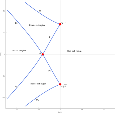
Figure 1. The phase diagram of the complex quartic random matrix model in the $\sigma$-plane. This phase diagram first appeared in the work [Dav91] of David. The Painlevé II double scaling limit corresponding to the multi-critical point $\sigma=-2$ was studied in [BI03], while the Painlevé I double scaling limit associated to the multi-critical points $\sigma=\pm\textrm{i}\sqrt{12}$ was investigated in [DK06]. The borders labeled by $\gamma_{1}$ through $\gamma_{4}$ separating the one-cut region from the three-cut region are the same lines shown in Figure 13 by labels I, XII, VII, and IX; and the borders labeled by $\gamma_{5}$ and $\gamma_{6}$ separating the two-cut region from the three-cut region are the same lines shown in Figure 15 by labels 1 and 2.

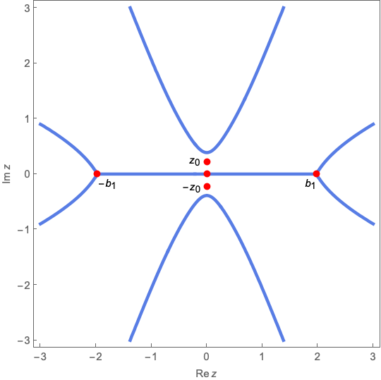
(a) $\mathscr{J}^{(1)}_{\sigma_{1}}$ at $\sigma_{1}=-1.9$.

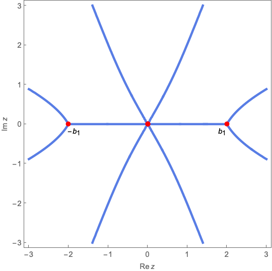
(b) $\mathscr{J}^{(1)}_{\sigma_{\mbox{\tiny cr}}}$ (or $\mathscr{J}^{(2)}_{\sigma_{\mbox{\tiny cr}}}$) at $\sigma_{\mbox{\tiny cr}}=-2$

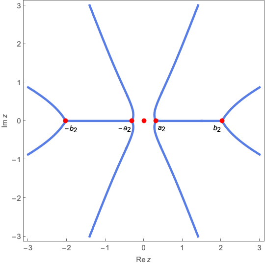
(c) $\mathscr{J}^{(2)}_{\sigma_{2}}$ at $\sigma_{2}=-2.1$

Figure 6. Snapshots of the continuous evolution of the critical graph $\mathscr{J}^{(1)}_{\sigma_{1}}$ to the critical graph $\mathscr{J}^{(2)}_{\sigma_{2}}$ as $\sigma$ varies from $\sigma_{1}=-1.9$ to $\sigma_{2}=-2.1$ through the multi-critical point $\sigma_{\mbox{\tiny cr}}=-2$ (locate the $\sigma$-values in Figure 1). At the critical value, just before the split, the point $z_{0}$ gets trapped at the origin between different portions of the critical graph.

The phase diagram of the complex quartic matrix model first appeared in the work [Dav91] of David (See Figure 1 below and Figure 5 of [Dav91]). Later in the work [BT15], Bertola and Tovbis found the phase diagram in the two-sheeted $u$-plane based on numerical computations, which under the change of parameters (1.13) is equivalent to Figure 1 (See Figure 6 in [BT15]). They also considered several other cases for the contour of integration in (1.5) other than the real axis, and among other things, in each case found the phase diagram (see Figures 4 through 9 in [BT15]) by computer-assisted methods. In [BT15] the authors did not provide a rigorous description of the phase diagram characterizing the boundaries of regions with different numbers of cuts. However, in [BT16], they developed such an analysis for a different configuration of contours of orthogonality, obtained explicit equations which provide an implicit characterization of the boundaries, and a proof that the regular case is open with respect to the parameters.

In the present work, one objective is to provide an explicit characterization of all the boundary curves shown in Figure 1, in terms of critical trajectories of new auxiliary quadratic differentials in the parameter space, originally discovered in [BDY17] for the case of a cubic potential. Along the way we do provide an independent proof that the regular one-cut, two-cut, and three-cut regimes are open, which is more straightforward than the approach of [BT16] because it is tailored to the quartic situation.

The phase diagram of the matrix model with the quartic polynomial $V(z;\sigma)$ on the complex plane $\sigma\in{\mathbb{C}}$ is described in terms of the underlying equilibrium measure

(1.20) $$\textrm{d}\nu_{\rm eq}(z;\sigma)=\frac{1}{\pi\textrm{i}}\,[Q(z;\sigma)^{1/2}]_{+}\textrm{d}z.$$

Here $Q(z;\sigma)$ is a polynomial in $z$ of degree 6 and the intervals of the support of the equilibrium measure (the cuts) are critical trajectories of the quadratic differential $Q(z;\sigma)\,\textrm{d}z^{2}$. See the work of Kuijlaars and Silva [KS15] and §3 below. For the quartic polynomial (1.15) the equilibrium measure can have 1, 2, or 3 cuts. See the works of Bertola and Tovbis [BT15, BT16] and §3 below. Figure 1 depicts the phase regions on the complex plane $\sigma$ corresponding to different numbers of cuts. There are three critical points on the phase diagram,

(1.21) $$\sigma_{1}=-2\quad\textrm{ and}\quad\sigma_{2,3}=\pm\sqrt{12}\,\textrm{i},$$

and six critical curves, separating different phase regions. We will denote by $\mathcal{C}[a,b]$ a critical curve connecting the points $a$ and $b$. We will also denote by $\mathcal{C}[a,e^{\textrm{i}\theta}\infty]$ a critical curve which goes from the point $a$ to $\infty$ on the complex plane approaching the direction with angle $\theta$ at infinity.

Observe that the phase diagram is symmetric with respect to the real axis $\sigma$, and the critical curves on the phase diagram are of the two types:

1. split of a cut, and

2. birth of a cut.

Notice that on the phase diagram 1 the curves

(1.22) $$\gamma_{1,2}=\mathcal{C}[-2,\pm\sqrt{12}\,\textrm{i}]$$

correspond to the split of a cut, and the ones

(1.23) $$\gamma_{3,4}=\mathcal{C}[\pm\sqrt{12}\,\textrm{i},e^{\pi\mp\pi/4}\infty],\quad\gamma_{5,6}=\mathcal{C}[-2,e^{\pi\mp\pi/4}\infty],$$

to the birth of a cut.

Our first main result in this paper is a description of the critical curves $\gamma_{1},\ldots,\gamma_{6}$ in terms of critical trajectories of some auxiliary quadratic differentials. We will denote by $\Gamma[a,b]$ a trajectory of a quadratic differential connecting the points $a$ and $b$.

Theorem 1.1.

Part I. Critical curves separating one-cut and three-cut regions. Let us make the substitution

(1.24) $$\sigma=-\frac{3\beta}{4}+\frac{4}{\beta}\,.$$

Then the critical curves $\gamma_{1},\gamma_{2},\gamma_{3},\gamma_{4}$ mapped to the $\beta$-plane are critical trajectories of the quadratic differential $\Xi(\beta){\textrm{d}}\beta^{2}$, where

(1.25) $$\Xi(\beta)=-\frac{(3\beta^{2}+16)^{3}(\beta^{2}-16)}{1024\,\beta^{6}}\,.$$

Part II. Critical curves separating two-cut and three-cut regions. The curves $\gamma_{5}$ and $\gamma_{6}$ are critical trajectories of the quadratic differential $\Upsilon(\sigma){\textrm{d}}\sigma^{2}$, where

(1.26) $$\Upsilon(\sigma)=\frac{\sigma^{2}}{4}-1.$$

Let us comment on Theorem 1.1. According to formula (1.25), the quadratic differential $\Xi(\beta){\textrm{d}}\beta^{2}$ has five finite critical points: one pole, $\beta_{0}=0$, and four zeros, $\beta_{1},\beta_{2},\beta_{3},\beta_{4}$, where

(1.27) $$\beta_{1,2}=\pm 4,\quad\beta_{3,4}=\pm\frac{4\textrm{i}}{\sqrt{3}}\,,$$

as shown in Figure 12. The pole $\beta_{0}$ is of degree 6, the zeros $\beta_{3,4}=\displaystyle\pm\frac{4\textrm{i}}{\sqrt{3}}$ are of degree 3, and the zeros $\beta_{1,2}=\pm 4$ of degree 1. Correspondingly, there are five critical trajectories of the quadratic differential emanating from $\beta_{3}$ and $\beta_{4}$, at the angle of $72^{\circ}$ to each other, and there are three critical trajectories emanating from each of the simple critical points, $\beta_{1}$ and $\beta_{2}$, at the angle of $120^{\circ}$ to each other. Finally, there are four critical trajectories emanating from the origin, at the angle of $90^{\circ}$ to each other. See Figure 12.

Observe that substitution (1.24) is a scaled Joukowski transformation. It maps the points as follows:

(1.28) $$\beta=\pm 4\mapsto\sigma=\mp 2,\quad\beta=\pm\frac{4\textrm{i}}{\sqrt{3}}\mapsto\sigma=\mp\sqrt{12}\,\textrm{i}\,.$$

Respectively, it maps the critical trajectories of the quadratic differential $\Xi(\beta)\textrm{d}\beta^{2}$ to the critical curves as follows:

(1.29) $$\Gamma\left[4,\mp\frac{4\textrm{i}}{\sqrt{3}}\right]\to\mathcal{C}\left[-2,\pm\sqrt{12}\,\textrm{i}\right]=\gamma_{1,2},$$

$$\Gamma\left[\mp\frac{4\textrm{i}}{\sqrt{3}},0\right]\;(\Re\beta\geq 0)\to\mathcal{C}[\pm\sqrt{12}\,\textrm{i},e^{\pi\mp\pi/4}\infty]=\gamma_{3,4}.$$

This gives the critical curves $\gamma_{1},\gamma_{2},\gamma_{3},\gamma_{4}$ as the Joukowski type map of the critical trajectories of the quadratic differential $\Xi(\beta)\textrm{d}\beta^{2}$. Observe that the one-cut region on the $\beta$-plane is bounded by the trajectories

$$\Gamma\left[4,\pm\frac{4\textrm{i}}{\sqrt{3}}\right]\quad\textrm{and}\quad\Gamma\left[\pm\frac{4\textrm{i}}{\sqrt{3}},0\right]\;(\Re\beta\geq 0).$$

See Figure 12.

Furthermore, the critical curves $\gamma_{5},\;\gamma_{6}$, separating two-cut and three-cut regions, are critical trajectories of the quadratic differential $\Upsilon(\sigma)\textrm{d}\sigma^{2}$, where $\Upsilon(\sigma)$ is given in (1.26). Observe that $\Upsilon(\sigma)$ has two simple critical points $\sigma_{1,2}=\pm 2$, and the critical curves $\gamma_{5},\;\gamma_{6}$ are the critical trajectories of the quadratic differential $\Upsilon(\sigma)\textrm{d}\sigma^{2}$ labeled by $1$ and $2$ in Figure 15. We prove Theorem 1.1 in §4.

Our second main result in this paper, which we prove in §3, is a description of the equilibrium measure in different phase regions on the phase diagram.

Theorem 1.2.

Part I. One-cut region. Let $\mathcal{O}_{1}$ be the open set on the complex plane $\sigma$ lying to the right of the curves $\gamma_{1},\;\gamma_{2},\gamma_{3}$, and $\gamma_{4}$, see Figure 1. Then for all $\sigma\in\mathcal{O}_{1}$

1. The equilibrium measure $\nu_{\rm eq}=\nu_{\rm eq}(\sigma)$ is regular.

2. $\nu_{\rm eq}$ has a one-cut support $\Gamma[-b_{1},b_{1}]$ which is a critical trajectory of the quadratic differential $(z^{2}-z_{0}^{2})^{2}(z^{2}-b_{1}^{2}){\textrm{d}}z^{2}$.

3. The critical points $b_{1}$ and $z_{0}$ of this quadratic differential depend analytically on $\sigma\in\mathcal{O}_{1}$.

Part II. Two-cut region. Let $\mathcal{O}_{2}$ be the open set on the complex plane $\sigma$ lying to the left of the curves $\gamma_{5},\;\gamma_{6}$, see Figure 1. Then for all $\sigma\in\mathcal{O}_{2}$

1. The equilibrium measure $\nu_{\rm eq}=\nu_{\rm eq}(\sigma)$ is regular.

2. $\nu_{\rm eq}$ has a two-cut support $\Gamma[-b_{2},-a_{2}]\cup\Gamma[a_{2},b_{2}]$ where the support cuts are critical trajectories of the quadratic differential $z^{2}(z^{2}-a_{2}^{2})(z^{2}-b_{2}^{2}){\textrm{d}}z^{2}$.

3. The critical points $a_{2}$ and $b_{2}$ of this quadratic differential depend analytically on $\sigma\in\mathcal{O}_{2}$.

Part III. Three-cut region. Let $\mathcal{O}_{3}$ be the open set on the complex plane $\sigma$ consisting of two connected components, $\mathcal{O}_{3}=\mathcal{O}_{31}\cup\mathcal{O}_{32}$, lying to the left of the curves $\gamma_{1},\;\gamma_{3},\;\gamma_{5}$ and $\gamma_{2},\;\gamma_{4},\;\gamma_{6}$, see Figure 1. Then for all $\sigma\in\mathcal{O}_{3}$

1. The equilibrium measure $\nu_{\rm eq}=\nu_{\rm eq}(\sigma)$ is regular.

2. $\nu_{\rm eq}$ has a three-cut support $\Gamma[-c_{3},-b_{3}]\cup\Gamma[-a_{3},a_{3}]\cup\Gamma[a_{3},b_{3}]$, where the support cuts are critical trajectories of the quadratic differential $(z^{2}-a_{3}^{2})(z^{2}-b_{3}^{2})(z^{2}-c_{3}^{2}){\textrm{d}}z^{2}$.

Remark 1.3.

In fact $\Re a_{3},\Im a_{3},\Re b_{3},\Im b_{3},\Re c_{3}$ and $\Im c_{3}$ are real-analytic functions of $\Re\sigma$ and $\Im\sigma$ for all $\sigma\in\mathcal{O}_{3}$. In [BBG⁺22], in the more general context where the external field is of even degree $2p$, $p\in{\mathbb{N}}$, among other things we establish the real-analyticity of the real and imaginary parts of the end-points for all $q$-cut regimes, $1\leq q\leq 2p-1$, with respect to the real and imaginary parts of the complex parameters in the external field.

1.2. Topological Expansion of the Free Energy and Combinatorics of Four-valent Graphs

Our third main result in this paper concerns the topological expansion of the free energy,

(1.30) $$F_{NN}(\sigma)=\frac{1}{N^{2}}\ln\frac{Z_{NN}(\sigma)}{{\mathcal{Z}}_{NN}^{\rm GUE}}\,.$$

The existence of the $\displaystyle\frac{1}{N^{2}}$ expansion of the free energy for general real potentials

$$\mathscr{V}(z)=\frac{z^{2}}{2}+\sum^{\nu}_{k=1}u_{k}z^{k},$$

is proven in [EM03], where $u_{k}\in{\mathbb{R}}$ are such that the corresponding partition function exists. The analogous result for the complex cubic potential $\mathscr{V}(z)=\frac{z^{2}}{2}+uz^{3}$ was proven in [BD12], and in this work we extend this result for the complex quartic potential (1.2), or equivalently for (1.15).

Theorem 1.4.

For all $\sigma$ in the one-cut region $\mathcal{O}_{1}$, the free energy $F_{NN}(\sigma)$ admits the topological expansion,

(1.31) $$F_{NN}(\sigma)\sim\sum_{g=0}^{\infty}\frac{f_{2g}(\sigma)}{N^{2g}}\,,$$

and the functions $f_{2g}(\sigma)$ are analytic in $\sigma$ for all $\sigma\in\mathcal{O}_{1}$.

Remark 1.5.

Due to (1.19), we also have

(1.32) $$\mathscr{F}_{NN}(u)\sim\sum_{g=0}^{M}\frac{\mathcal{f}_{2g}(u)}{N^{2g}}\,.$$

In §6 we show that the coefficients $\mathcal{f}_{2g}(u)$ are analytic functions of $u$ in a neighborhood of the origin independent of $g$, more precisely in a disk of radius $\frac{1}{12}$.

As mentioned before, (1.32) is referred to as the topological expansion of the partition function. Roughly, the quest for models of quantum gravity led to the 2-dimensional reduction in which large but finite collections of different geometries on Riemann surfaces are considered, and one seeks a natural probability measure on these geometries. F. David [Dav85] and V. Kazakov [Kaz85] first introduced such random surfaces discretized using polygons to define models of two-dimensional quantum gravity, making use of the connection between graphical enumeration and integrals over large matrices discovered by t’Hooft [tH74]. To understand the probability measure, one needs to know how many of these geometries there are, and the problem in enumerative geometry that emerges is to count the number of graphs that can be embedded into a Riemann surface, according to the genus of the surface and the number of vertices of different valences. As discovered in the subsequent works [BIPZ78], [Bes79] and [BIZ80], the topological expansion above should be an expansion of generating functions, in which $\mathcal{f}_{2g}(u)$ is a combinatorial generating function whose $j$-th coefficient yields the number of labelled graphs with $j$ vertices of valence 4, that can be embedded in a Riemann surface of genus $g$. Yet another connection was discovered by Witten [Wit91], to the intersection theory of the moduli space of Riemann surfaces, where intersection numbers can also be computed using matrix integrals.

Since the emergence of rigorous mathematical analysis of the partition function by Riemann-Hilbert methods in [EM03] and in [BI05], there have followed works aimed at extracting explicit information about the generating functions and about the important combinatorial coefficients. For example, in [EMP08] the authors initiated an investigation of the generating functions in the topological expansion in the case that all vertices were of a fixed, even, valence. They made use of both the Toda equations and the string equations, and provided a description of structural properties of the generating functions in terms of inversion of certain differential operators. They extracted some explicit information for enumeration of maps on surfaces of genus $0$, $1$, and $2$, along with recursive definitions for higher genus. (Explicit representation of the generating function means a complete solution of the combinatorial problem for each genus and maps of a fixed valence type.) Later, Ercolani [Erc11, Erc14] continued this research, analyzing a hierarchy of partial differential equations coming from the Toda lattice equations (and the asymptotic expansion of the partition function) and derived semi-explicit characterizations of the $\mathcal{f}_{2g}(u)$ as rational functions of other auxiliary functions.

As already mentioned above, for the three-valent case (the cubic matrix model), the Riemann-Hilbert analysis and topological expansion were established in [BD12] and [BDY17], where in particular the authors explicitly evaluated the combinatorial coefficients explicitly for genus $0$ and $1$. Characterization results for the generating functions for other odd valences have recently been obtained by Ercolani and Waters [EW21].

An interesting difference in approach between the present work and the works [Erc11, Erc14, EMP08, EW21] is the following: we exploit the string equation and a (possibly new) explicit equation for the first derivative of the free energy (6.2) to obtain recursive relations, whereas in the works of Ercolani and collaborators, they use the string equation and a hierarchy of partial differential equations derived from the Toda lattice system of ordinary differential equations. At present our equation for the first derivative of the free energy is only known for the quartic model, while the analysis of Ercolani and collaborators works for more general single valence settings.

In §6 we establish a number of results concerning these generating functions. We provide recursive relations in $g$, as well as explicit representations for $g=0,1,2,$ and $3$. The representations (6.140), (6.141), and (6.142) respectively for $g=0,1$, and $2$ agree with the classical paper of Bessis, Itzykson, and Zuber [BIZ80], while we believe the result for $g=3$ is new. As with other representations, the recursive algorithm does yield explicit representations for any genus, but requires more effort as the genus increases. To that end, let us highlight the following result regarding enumeration of graphs.

Theorem 1.6.

Let $\mathscr{N}_{j}(g)$ be the number of connected labeled 4-valent graphs with $j$ vertices which are realizable on a closed Riemann surface of genus $g$ , but not realizable on Riemann surfaces of lower genus. For the Riemann surface of genus three we have

(1.33) $$\begin{split}\mathscr{N}_{j+4}(3)&=\frac{16\cdot 48^{j}\left(j+3\right)!}{3(j)!}\times\\ &\left(\frac{2741}{10}(j+5)!-\frac{291}{10}j(j+4)!-\frac{2741}{1260}\frac{(2j+9)!}{4^{j}(j+4)!}-\frac{292j(2j+7)!}{315\cdot 4^{j}(j+3)!}\right),\quad j\in{\mathbb{N}},\end{split}$$

where $\mathscr{N}_{1}(3)=\mathscr{N}_{2}(3)=\mathscr{N}_{3}(3)=\mathscr{N}_{4}(3)=0$, that is to say all connected labeled 4-valent graphs with $1,2,3,$ or $4$ vertices can be realized on the sphere, torus, or the two-holed torus.

We also highlight a result that describes the asymptotic behavior of the number of four-valent graphs on a Riemann surface of arbitrary genus $g$, as the number of vertices grows to infinity. The following result is basically a corollary of Theorem 6.8.

Theorem 1.7.

The asymptotics of the number of connected labeled $4$-valent graphs on a Riemann surface of genus $g\in{\mathbb{N}}\cup\{0\}$, as the number of vertices tends to infinity, is given by

(1.34) $$\mathscr{N}_{j}(g)=\mathcal{K}_{g}48^{j}j!j^{\frac{5g-7}{2}}\left(1+O(j^{-1/2})\right),\qquad j\to\infty,$$

where the constants $\mathcal{K}_{g}$ are the same as the ones in Theorem 6.8:

(1.35) $$\mathcal{K}_{g}=\begin{cases}\displaystyle\frac{12^{\frac{5g-1}{2}}}{\left(\frac{5g-5}{2}\right)!}\frac{1}{5g-3}\mathcal{C}_{2g},&g=2k+1,\\[10.0pt] \displaystyle\frac{12^{\frac{5g-1}{2}}2^{5g-4}}{\sqrt{\pi}}\frac{\left(\frac{5g-4}{2}\right)!}{\left(5g-3\right)!}\mathcal{C}_{2g},&g=2k,\end{cases}\qquad k\in{\mathbb{N}},$$

while $\mathcal{K}_{0}=2^{-1}\pi^{-1/2}$, and $\mathcal{K}_{1}=24^{-1}$, where the constants $\mathcal{C}_{2g}$ can be found recursively from the following relations

(1.36) $$\mathcal{C}_{2g}=\frac{1}{2^{3}3^{\frac{1}{2}}}\sum^{g-1}_{\ell=1}\mathcal{C}_{2g-2\ell}\mathcal{C}_{2\ell}+\frac{(5g-6)(5g-4)}{2^{8}3^{\frac{7}{2}}}\mathcal{C}_{2g-2},\qquad\mathcal{C}_{0}=-2^{2}3^{\frac{1}{2}},\qquad g\in{\mathbb{N}}.$$

Remark 1.8.

It is worth noticing that the constants $\mathcal{C}_{2g}$ also arise in the asymptotic expansion of the one-parameter family of the Boutroux tronquée solutions $u(\tau)=u(\tau;\alpha)$ to the Painlevé I equation

$$u^{\prime\prime}(\tau)=6u^{2}(\tau)+\tau$$

as $\tau\to-\infty$. Namely, as $\tau\to-\infty$,

$$u(\tau;\alpha)\sim\sqrt{-\frac{\tau}{6}}\,\sum_{k=0}^{\infty}a_{k}(-\tau)^{-5k/2},$$

where the coefficients $a_{k}$ do not depend on the parameter $\alpha$, and they are given by the nonlinear recursion

(1.37) $$a_{0}=1,\quad a_{k+1}=\frac{25k^{2}-1}{8\sqrt{6}}\,a_{k}-\frac{1}{2}\sum_{m=1}^{k}a_{m}a_{k+1-m}$$

(see, e.g., the works [BDn16, Bou13, CCH15, Erc11, Erc14, Kap04]). Define now the rescaled Boutroux functions

$$y(t)=-2^{8/5}3^{2/5}u(-2^{9/5}3^{6/5}t).$$

Then it can be checked directly, by using (1.37), that as $t\to\infty$,

$$y(t)\sim\sum_{g=0}^{\infty}\mathcal{C}_{2g}t^{(1-5g)/2},$$

where the coefficients $\mathcal{C}_{2g}$ are given by nonlinear recursion (1.36). Therefore, the coefficients $\mathcal{C}_{2g}$ coincide with the coefficients of the asymptotic expansion of the rescaled Boutroux functions $y(t)$ as $t\to\infty$.

The appearance of the Boutroux tronquée solutions can be explained as follows. Under the substitution $u=\sigma^{-2}$ (see formula (1.13)), the critical points $\sigma=\pm\textrm{i}\sqrt{12}$ and $\sigma=-2$ on the phase diagram, depicted on Figure 1 above, are mapped to the points $u=-\frac{1}{12}$ and $u=\frac{1}{4}$, respectively. The point $u=-\frac{1}{12}$ is closer to the origin than the one $u=\frac{1}{4}\,,$ and it determines the asymptotic behavior of the Taylor coefficients of the functions $f_{2g}(u)$ at the origin. But as shown in the paper [DK06] of Duits and Kuijlaars, the double scaling limit of the model at the critical point $u=-\frac{1}{12}$ is described in terms of a Boutroux tronquée solution to the Painlevé I equation. It is noteworthy that the double scaling limit of the matrix model at the critical point $u=-\frac{1}{12}$ gives rise to the 2D continuous quantum gravity of Polyakov (see, e.g., the papers [DFGZJ95] and [Wit91], and references therein).

Remark 1.9.

The formula (1.34) was formulated as a conjecture in the introduction of [FIKN06] (see pages 27 through 29 of [FIKN06] for the relevant references). Here we directly quote from [FIKN06]:

“The status of

$$\mathscr{N}_{j}(g)\sim\mathcal{K}_{g}48^{j}j!j^{\frac{5g-7}{2}}$$

remains that of a conjecture. Nevertheless, the current level of development of the Riemann-Hilbert techniques, and the experience with other combinatorial problems e.g. in random permutations [BDJ99], suggest that all the gaps in the above construction will be soon filled.”

Indeed in Theorem 1.7 above we have not only established this conjecture, but furthermore we have also characterized the constants $\mathcal{K}_{g}$ explicitly in terms of the constants $\mathcal{C}_{2g}$. It should be mentioned that in the recent preprint [EW21] mentioned above, the authors provide an analogue of (1.34) and (1.35) for the general single even-valence potential. The result in the preprint is stated for even numbers of vertices (see equation A.9 of [EW21]), but by comparing to our result the form of the asymptotics surely holds for both even and odd numbers of vertices. They omit the proof, but presumably it follows from a similar analysis done in the same paper for a different combinatorial problem (see Corollary 10.8 of [EW21]).

Remark 1.10.

A very interesting direction of research is to explore the precise connection between the asymptotics of the labeled graphs embedded on a Riemann surface of genus $g$ as the number of vertices go to infinty (as addressed in Theorem 1.7 for the four-valent case, and in Theorem 1.4 of [BD12] for the three-valent case) and the asymptotics of the number of the so-called rooted maps as the number of edges goes to infinity.

Let us recall some definitions regarding the latter asymptotics from [BGR08]. Let $\Sigma_{g}$ be the orientable surface of genus $g$. A map on $\Sigma_{g}$ is a graph $G$ embedded on $\Sigma_{g}$ such that all components of $\Sigma_{g}\setminus G$ are simply connected regions. These components are called faces of the map. A map is rooted by distinguishing an edge, an end vertex of the edge and a side of the edge. Let us denote by $M_{n,g}$ the number of rooted maps on $\Sigma_{g}$ with $n$ edges. In [BC86] Bender and Canfield showed that

(1.38) $$M_{n,g}\sim t_{g}n^{\frac{5g-5}{2}}12^{n}\quad\text{as}\quad n\to\infty,$$

where the $t_{g}$ are positive constants which can be calculated recursively. One can already observe the apparent similarity between (1.38) and (1.34), which becomes even more interesting when one observes that the first three values for $t_{g}$ are given in [BC86] by

$$t_{0}=\frac{2}{\sqrt{\pi}}\equiv 4\mathcal{K}_{0},\qquad t_{1}=\frac{1}{24}\equiv\mathcal{K}_{1},\quad\text{and}\quad t_{2}=\frac{7}{4320\sqrt{\pi}}\equiv\frac{1}{4}\mathcal{K}_{2}.$$

An analogous similarity can also be seen when one compares (1.38) with equation 1.25 of [BD12] which gives the asymptotics of the number of labeled three-valent graphs as the number of vertices goes to infinity. For the asymptotics of the rooted maps see also the works [BC86, BGR08, Gao91, Gao93, GLMn08] and references therein.

1.3. Outline

The paper is organized as follows:

• In §2 we derive the end-point equations in the one-cut, two-cut, and three-cut regimes. These endpoint equations are algebraic in the one-cut and two-cut case, thereby allowing for explicit solutions. In the one-cut and two-cut cases we find explicit expressions for the $g$-function and the Euler-Lagrange constants.

• In §3 we prove results about the structure of critical graphs in the $z$-plane using the theory of quadratic differentials. We also prove the openness of one-cut, two-cut, and three-cut regimes.

• In §4 we use auxiliary quadratic differentials to prove the phase diagram as depicted in Figure 1.

• In §5 we prove the topological expansion of the recurrence coefficients of the orthogonal polynomials using the Riemann-Hilbert analysis and the String equations.

• In §6 we derive the Toda equations. We use the equation for $\mathcal{F}^{\prime}$ to prove the topological expansion for the free energy. As a result we extract the combinatorial information about the connected labeled $4$-valent graphs Riemann surfaces of various genera.

• Finally in the Appendix 7 we provide visual illustrations of four valent graphs on the sphere and the torus with one and two vertices. We hope this helps for a deeper understanding of the combinatorial formulae (6.140) through (6.143).

2. Equilibrium Measure

In this section we first discuss the equilibrium measure for a general complex polynomial $V(z)$, and then we will specify it to the equilibrium measure of the quartic complex polynomial (1.15).

2.1. Equilibrium Measure for a General Complex Polynomial.

Let

(2.1) $$V(z)=\frac{z^{2p}}{2p}+\sum_{j=1}^{2p-1}\frac{v_{j}z^{j}}{j}$$

be a polynomial of even degree $2p$ with the leading coefficient $\displaystyle\frac{1}{2p}$ and complex coefficients $\displaystyle\frac{v_{j}}{j}\,,\;j=1,\ldots,2p-1$. We follow the work of Kuijlaars and Silva [KS15], also see the works [Rak12], [MFR11], [Ber11].

For a given $\varepsilon$, such that

$$\frac{\pi}{4p}>\varepsilon>0,$$

consider the sectors

(2.2) $$S^{+}_{\varepsilon} =\left\{z\in{\mathbb{C}}\;\Big{|}\;|\arg z|\leq\frac{\pi}{4p}-\varepsilon\right\},$$

$$S^{-}_{\varepsilon} =\left\{z\in{\mathbb{C}}\;\Big{|}\;|\arg z-\pi|\leq\frac{\pi}{4p}-\varepsilon\right\}.$$

Observe that in these sectors,

(2.3) $$\lim_{z\to\infty}\Re V(z)=\infty.$$

Let us define a class $\mathcal{T}$ of admissible contours on the complex plane. By a contour we mean a continuous curve $z=z(t)$, $-\infty<t<\infty$, without self-intersections. We say that a contour $\Gamma$ is admissible if

1. The contour $\Gamma$ is a finite union of $C^{1}$ Jordan arcs.

2. There exists $\varepsilon>0$ and $r_{0}>0$, such that $\Gamma$ goes from $S^{-}_{\varepsilon}$ to $S^{+}_{\varepsilon}$ in the sense that $\forall\,r>r_{0},$ $\exists\,t_{0}<t_{1}$ such that

   $$z(t)\in S^{-}_{\varepsilon}\setminus D_{r}\quad\forall\,t<t_{0};\quad z(t)\in S^{+}_{\varepsilon}\setminus D_{r}\quad\forall\,t>t_{1},$$

   where $D_{r}$ is the disk centered at the origin with radius $r$. We will assume that the contour $\Gamma$ is oriented from $(-\infty)$ to $(+\infty)$, where $(-\infty)$ lies in the sector $S^{-}_{\varepsilon}$ and $(+\infty)$ in the sector $S^{+}_{\varepsilon}$. The orientation defines an order on the contour $\Gamma$.

An example of an admissible contour is the real line.

Let $\Gamma\in\mathcal{T}$ be an admissible contour and $\mathcal{P}(\Gamma)$ the space of probability measures $\nu$ on $\Gamma$ such that

(2.4) $$\underset{\Gamma}{\int} |\Re V(s)|\,\textrm{d}\nu(s)<\infty.$$

Consider the following real-valued functional on $\mathcal{P}(\Gamma)$:

(2.5) $$I_{V,\Gamma}(\nu):=\underset{\Gamma\,\times\,\Gamma}{\iint}\log\frac{1}{|z-s|}\,\textrm{d}\nu(z)\textrm{d}\nu(s)+\int_{\Gamma}\Re V(s)\,\textrm{d}\nu(s).$$

Then there exists a unique minimizer $\nu_{V,\Gamma}$ of the functional $I_{V,\Gamma}(\nu)$, so that

(2.6) $$\min_{\nu\in\mathcal{P}(\Gamma)}I_{V,\Gamma}(\nu)=I_{V,\Gamma}(\nu_{V,\Gamma}).$$

See the work [ST97].

The probability measure $\nu_{V,\Gamma}$ is called the equilibrium measure of the functional $I_{V,\Gamma}(\nu)$. The support of $\nu_{V,\Gamma}$ is a compact set $J_{V,\Gamma}\subset\Gamma$. An important fact is that the equilibrium measure is uniquely determined by the Euler–Lagrange variational conditions. Namely, $\nu_{V,\Gamma}$ is the unique probability measure $\nu$ on $\Gamma$ such that there exists a constant $l$, a Lagrange multiplier, such that

(2.7) $$U^{\nu}(z)+\frac{1}{2}\,\Re V(z)=\ell,\quad z\in\textrm{supp}\,\nu,$$

$$U^{\nu}(z)+\frac{1}{2}\,\Re V(z)\geq\ell,\quad z\in\Gamma\setminus\textrm{supp}\,\nu,$$

where

(2.8) $$U^{\nu}(z)=\int_{\Gamma}\log\frac{1}{|z-s|}\,\textrm{d}\nu(s)$$

is the logarithmic potential of the measure $\nu$ [ST97].

Now we maximize $I_{V}(\nu_{V,\Gamma})$ over $\Gamma\in\mathcal{T}$. The main result of the work of Kuijlaars and Silva concerns the existence and properties of the maximizing contour $\Gamma_{0}\in\mathcal{T}$. They prove that the maximizing contour $\Gamma_{0}\in\mathcal{T}$ exists, and the equilibrium measure

$$\nu_{\rm eq}=\nu_{V,\Gamma_{0}}$$

on $\Gamma_{0}$ is supported by a set $J\subset\Gamma_{0}$ which is a finite union of analytic arcs $\Gamma_{0}[a_{k},b_{k}]\subset\Gamma_{0},\;k=1,\ldots,q$,

$$J=\bigcup_{k=1}^{q}\Gamma_{0}[a_{k},b_{k}],\quad a_{1}<b_{1}\leq a_{2}<b_{2}\leq\ldots\leq a_{q}<b_{q},$$

that are critical trajectories of a quadratic differential $Q(z)\,\textrm{d}z^{2}$ (see the beginning of §3 for a review of definitions and basic facts about quadratic differentials), where $Q(z)$ is a polynomial of degree

(2.9) $$\deg Q(z)=2\deg V(z)-2=4p-2.$$

Furthermore, Kuijlaars and Silva prove that the polynomial $Q(z)$ is equal to

(2.10) $$Q(z)=\left(-\omega(z)+\frac{V^{\prime}(z)}{2}\right)^{2},$$

where

(2.11) $$\omega(z)=\int_{J}\frac{\textrm{d}\nu_{\rm eq}(s)}{z-s}$$

is the resolvent of the measure $\nu_{0}$. Expanding

$$\frac{1}{z-s}=\frac{1}{z}+\frac{s}{z^{2}}+\frac{s^{2}}{z^{3}}+\ldots,$$

we obtain that as $z\to\infty$,

(2.12) $$\omega(z)=\frac{1}{z}+\frac{m_{1}}{z^{2}}+\ldots,\quad m_{k}=\int_{J}s^{k}\textrm{d}\nu_{\rm eq}(s).$$

In addition, the equilibrium measure $\nu_{\rm eq}$ is absolutely continuous with respect to the arc length and

(2.13) $$\textrm{d}\nu_{\rm eq}(s)=\frac{1}{\pi\textrm{i}}\,Q_{+}(s)^{1/2}\textrm{d}s,$$

where $Q_{+}(s)^{1/2}$ is the limiting value of the function

(2.14) $$Q(z)^{1/2}=-\int_{J}\frac{\textrm{d}\nu_{\rm eq}(s)}{z-s}+\frac{V^{\prime}(z)}{2},$$

as $z\to s\in J$ from the left-hand side of $J$ with respect to the orientation of the contour $\Gamma_{0}$ from $(-\infty)$ to $\infty$. Observe that as $z\to\infty$,

(2.15) $$Q(z)^{1/2}=-\left(\frac{1}{z}+\frac{m_{1}}{z^{2}}+\ldots\right)+\frac{1}{2}\left(z^{2p-1}+\sum_{j=1}^{2p-1}v_{j}z^{j-1}\right).$$

A very important result of Kuijlaars and Silva is that the equilibrium measure $\nu_{\rm eq}$ is unique as the max-min measure. On the other hand, the contour $\Gamma_{0}$ is not unique because it can be deformed outside of the support $J$ of $\nu_{\rm eq}$.

2.2. The $g$-function.

We define the $g$-function as

(2.16) $$g(z)=\int_{J}\log(z-s)\,\textrm{d}\nu_{\rm eq}(s),$$

where for a fixed $s\in J$, we consider a cut of $\log(z-s)$ on the part of the curve $\Gamma_{0}$ where $z<s$ with respect to the ordering on $\Gamma_{0}$. Observe that by (2.11),

(2.17) $$g^{\prime}(z)=\int_{J}\frac{\textrm{d}\nu_{\rm eq}(s)}{z-s}=\omega(z),$$

In addition, by (2.8), the logarithmic potential $U^{\nu_{\rm eq}}(z)$ is equal to

(2.18) $$U^{\nu_{\rm eq}}(z)=\int_{J}\log\frac{1}{|z-s|}\,\textrm{d}\nu_{\rm eq}(s)=-\Re g(z)$$

hence the Euler–Lagrange variational conditions (2.7) can be written as

(2.19) $$-\Re g(z)+\frac{1}{2}\,\Re V(z)=\ell,\quad z\in J,$$

$$-\Re g(z)+\frac{1}{2}\,\Re V(z)\geq\ell,\quad z\in\Gamma_{0}\setminus J.$$

2.3. Regular and Singular Equilibrium Measures

An equilibrium measure $\nu_{\rm eq}$ is called regular if the following three conditions hold:

1. The arcs $\Gamma_{0}[a_{k},b_{k}],\;k=1,\ldots,q,$ of the support of $\nu_{\rm eq}$ are disjoint.

2. The end-points $\{a_{k},b_{k},\;k=1,\ldots,q\}$ are simple zeros of the polynomial $Q(s)$.

3. There is a contour $\Gamma_{0}$ containing the support $J$ of $\nu_{\rm eq}$ such that

   (2.20) $$U^{\nu}(z)+\frac{1}{2}\,\Re V(z)>\ell,\quad z\in\Gamma_{0}\setminus J.$$

An equilibrium measure $\nu_{\rm eq}$ is called singular (or critical) if it is not regular.

2.3.1. Regular Equilibrium Measures

Suppose that an equilibrium measure $\nu_{\rm eq}$ is regular. Since the resolvent

(2.21) $$\omega(z)=\int_{J}\frac{\textrm{d}\nu_{\rm eq}(s)}{z-s}$$

is analytic on ${\mathbb{C}}\setminus J$, it follows from equation (2.10) that if the equilibrium measure $\nu_{0}$ is regular then all the zeros of the polynomial $Q(z)$ different from the end-points $\{a_{k},b_{k},\;k=1,\ldots,q\}$ are of even degree, hence $Q(z)$ can be written as

(2.22) $$Q(z)=\frac{1}{4}\,h(z)^{2}R(z),$$

where $h(z)$ is a polynomial,

(2.23) $$h(z)=\prod_{j=0}^{r}(z-z_{j}),$$

with zeroes $z_{0},\ldots,z_{r}$ different from the end-points $\{a_{k},b_{k},\;k=1,\ldots,q\}$, and

(2.24) $$R(z)=\prod_{k=1}^{q}(z-a_{k})(z-b_{k}).$$

Thus,

(2.25) $$Q(z)=\frac{1}{4}\,h(z)^{2}R(z)=\frac{1}{4}\prod_{j=0}^{r}(z-z_{j})^{2}\prod_{k=1}^{q}(z-a_{k})(z-b_{k}).$$

By taking the square root with the plus sign, we obtain that

(2.26) $$Q(z)^{1/2}=\frac{1}{2}\,h(z)R(z)^{1/2}=\frac{1}{2}\prod_{j=0}^{r}(z-z_{j})\left[\prod_{k=1}^{q}(z-a_{k})(z-b_{k})\right]^{1/2},$$

Correspondingly, equation (2.13) can be rewritten as

(2.27) $$\textrm{d}\nu_{\rm eq}(z) =\frac{1}{2\pi\textrm{i}}\,h(z)R_{+}(z)^{1/2}\textrm{d}z=\frac{1}{2\pi\textrm{i}}\,\prod_{j=0}^{r}(z-z_{j})\left[\prod_{k=1}^{q}(z-a_{k})(z-b_{k})\right]_{+}^{1/2}\textrm{d}z.$$

Now we will apply the above results for the equilibrium measure of a general complex polynomial $V(z)$ to the quartic polynomial

$$V(z)=V(z;\sigma)=\frac{z^{4}}{4}+\frac{\sigma z^{2}}{2}\,,\quad\sigma\in{\mathbb{C}}.$$

2.4. Equilibrium Measures for the Quartic Polynomials $V(z;\sigma)$

For the quartic polynomial in hand, equation (2.10) for the polynomial $Q(z)$ reads

(2.28) $$Q(z)=\left(-\omega(z)+\frac{z^{3}+\sigma z}{2}\right)^{2},\quad\omega(z)=\int_{J}\frac{\textrm{d}\nu_{\rm eq}(s)}{z-s}\,.$$

Since the polynomial $V(z)$ is even, the uniqueness of the equilibrium measure $\nu_{\rm eq}$ implies that

1. $\nu_{\rm eq}$ is even, $\nu_{\rm eq}(-s)=\nu_{\rm eq}(s)$.

2. The resolvent $\omega(z)$ is odd, $\omega(-z)=-\omega(z)$, and

3. The polynomial $Q(z)$ is even, $Q(-z)=Q(z)$.

Considering $z\to\infty$, we obtain that

(2.29) $$Q(z)=\left(\frac{z^{3}+\sigma z}{2}-\frac{1}{z}-\frac{m_{2}}{z^{3}}-\ldots\right)^{2}=\frac{1}{4}\big{[}z^{6}+2\sigma z^{4}+(\sigma^{2}-4)z^{2}-4(\sigma+m_{2})\big{]}.$$

Since $Q(z)$ is a polynomial of degree 6, the possible number of cuts $q$ in formula (2.25) can be $q=1,2,$ and $3$. Let us consider them in more detail.

2.4.1. One-Cut Equilibrium Measure

When $q=1$, formula (2.25) gives that

(2.30) $$Q(z)=\frac{1}{4}\,(z-z_{0})^{2}(z-z_{1})^{2}(z-a_{1})(z-b_{1}).$$

Since the equilibrium measure $\nu_{0}$ is even and the polynomial $Q(z)$ is even, we have that

(2.31) $$-a_{1}=b_{1},\quad-z_{1}=z_{0},$$

hence

(2.32) $$Q(z)=\frac{1}{4}\left(z^{2}-z_{0}^{2}\right)^{2}(z^{2}-b_{1}^{2}).$$

Equating this expression to the one (2.29), we obtain that

(2.33) $$(z^{2}-c^{2})^{2}(z^{2}-b^{2})=z^{6}+2\sigma z^{4}+(\sigma^{2}-4)z^{2}-4(\sigma+m_{2}).$$

Comparing the coefficients at $z^{4}$ and $z^{2}$, we obtain the system of equations,

(2.34) $$\left\{\;\begin{aligned} &b_{1}^{2}+2z_{0}^{2}=-2\sigma,\\ &2b_{1}^{2}z_{0}^{2}+z_{0}^{4}=\sigma^{2}-4.\end{aligned}\right.$$

From the first equation we have that

$$\sigma=-\frac{b_{1}^{2}}{2}-z_{0}^{2}.$$

Substituting this expression into the second equation and simplifying we obtain that

$$b_{1}^{2}(b_{1}^{2}-4z_{0}^{2})=16.$$

Thus, we have the system of equations,

(2.35) $$\left\{\;\begin{aligned} &b_{1}^{2}+2z_{0}^{2}=-2\sigma,\\ &b_{1}^{2}(b_{1}^{2}-4z_{0}^{2})=16.\end{aligned}\right.$$

Solving it we obtain that

(2.36) $$b_{1}^{2}=\frac{2}{3}\left(-\sigma\pm\sqrt{12+\sigma^{2}}\right)\quad\text{and}\quad z_{0}^{2}=\frac{1}{3}\left(-2\sigma\mp\sqrt{12+\sigma^{2}}\right).$$

As shown by Bleher and Its (see [BI99, BI03, BI05]), for real $\sigma>-2$, the one-cut equilibrium measure persists with a real $b_{1}>0$. This determines the sign in the latter formulae,

(2.37) $$b_{1}=\sqrt{\frac{2}{3}\left(-\sigma+\sqrt{12+\sigma^{2}}\right)}\quad\text{and}\quad z_{0}=\sqrt{\frac{1}{3}\left(-2\sigma-\sqrt{12+\sigma^{2}}\right)}.$$

Observe that for $\sigma=-2$, we have $b_{1}=2$ and $z_{0}=0$. Theorem 1.1 tells us that the point $\sigma=-2$ corresponds to a split of the cut $[-2,2]$ at $z_{0}=0$, when $\sigma$ is decreasing from $\sigma>-2$ to $\sigma<-2$. As shown in [BI03], the critical behavior of the quartic model at $\sigma=-2$ is governed by the Hastings-McLeod solution to the second Painlevé equation PII. In what follows we will show that formulae (2.37) are analytically extended from the real half-line $\sigma>-2$ to the whole one-cut region $\sigma\in\mathcal{O}_{1}$ on the complex plane.

Remark 2.1.

Notice that the branch cuts for $z_{0}(\sigma)$ and $b_{1}(\sigma)$ are different. Indeed for $b_{1}(\sigma)$, since $-\sigma+\sqrt{12+\sigma^{2}}\neq 0$ for all $\sigma$, there are only two branch cuts $L_{\pm}$ emanating from $\pm\textrm{i}\sqrt{12}$. However when we consider $z_{0}(\sigma)$, we notice that $-2\sigma-\sqrt{12+\sigma^{2}}$ does vanish for $\sigma=-2$. So, for $z_{0}(\sigma)$, apart from the two branch cuts emanating from $\pm\textrm{i}\sqrt{12}$ (which we chose to be $L_{\pm}$: the same as the ones for $b_{1}(\sigma)$) there is one more branch cut $L$ which emanates from $-2$. In this work we choose $L_{\pm}=\pm\textrm{i}\sqrt{12}-t$ and $L=-2-t$, $t>0$. We choose the branches so that for $\sigma>-2$:

$$z_{0}(\sigma)=\textrm{i}y_{0}\quad\mbox{with}\quad y_{0}>0,\qquad\quad\text{and}\quad\qquad b_{1}(\sigma)>0.$$

Since $z^{2}_{0}(\sigma)\in(0,\infty)$ for $\sigma\in(-\infty,-2)$, the branch cut in the $z_{0}^{2}$-plane is the positive real axis and we fix the branch of $z_{0}$ by fixing $0\leq\arg(z^{2}_{0})<2\pi$.

In the one-cut regime the $g$ function can be explicitly computed. To this end, using (2.10), (2.17), and (2.32) we can write

(2.38) $$g(z;\sigma)=\frac{V(z)+\ell^{(1)}_{*}}{2}+\frac{\eta_{1}(z;\sigma)}{2},\qquad z\in{\mathbb{C}}\setminus\Gamma_{\sigma}(-\infty,b_{1}],$$

where

(2.39) $$\eta_{1}(z;\sigma):=-\int^{z}_{b_{1}}(s^{2}-z^{2}_{0})\sqrt{s^{2}-b_{1}^{2}}\textrm{d}s,\qquad z\in{\mathbb{C}}\setminus\Gamma_{\sigma}(-\infty,b_{1}],$$

in which the path of integration does not cross $\Gamma_{\sigma}(-\infty,b_{1}(\sigma)]$. Notice that

(2.40) $$\eta_{1,+}(z)=-\eta_{1,-}(z),\qquad z\in J_{\sigma},$$

and

(2.41) $$\eta_{1,+}(z)-\eta_{1,-}(z)=4\pi\textrm{i},\qquad z\in\Gamma_{\sigma}(-\infty,-b_{1}).$$

Using several integration by parts and trigonometric substitutions we find

(2.42) $$\eta_{1}(z;\sigma)=\frac{z}{8}(b_{1}^{2}+4z^{2}_{0}-2z^{2})\sqrt{z^{2}-b_{1}^{2}}+2\log\left(\frac{z+\sqrt{z^{2}-b_{1}^{2}}}{b_{1}}\right),$$

where we have used (2.35) in simplifying the expression. Therefore we have the following explicit form of the $g$-function in the one-cut regime

(2.43) $$g(z;\sigma)=\frac{1}{2}\left(\frac{\sigma z^{2}}{2}+\frac{z^{4}}{4}+\ell^{(1)}_{*}\right)-\frac{z}{16}(b_{1}^{2}+4\sigma+2z^{2})\sqrt{z^{2}-b_{1}^{2}}+\log\left(\frac{z+\sqrt{z^{2}-b_{1}^{2}}}{b_{1}}\right),$$

where we have also used (2.35). Here the branches must be chosen to ensure that the branch cut for $g$ is $\Gamma_{\sigma}(-\infty,b_{1}]$. Also the constant $\ell_{*}^{(1)}$ can be found using the requirement that

$$g(z;\sigma)=\log z+\mathcal{O}(z^{-1})$$

as $z\to\infty$. Indeed,

(2.44) $$\ell^{(1)}_{*}=\frac{1}{12}\left(\sigma^{2}-\sigma\sqrt{12+\sigma^{2}}\right)+\log\left(-\sigma+\sqrt{12+\sigma^{2}}\right)-\frac{1}{2}-\log 6.$$

In what follows we use the notations

(2.45) $$\mathscr{G}^{(j)}_{1}(z;\sigma):=g_{+}(z;\sigma)-g_{-}(z;\sigma),$$

and

(2.46) $$\mathscr{G}^{(j)}_{2}(z;\sigma):=g_{+}(z;\sigma)+g_{-}(z;\sigma)-V(z;\sigma)-\ell^{(j)}_{*},$$

for $j=1,2$, and $3$, respectively associated with the one-cut, two-cut, and three-cut regimes. We have

(2.47) $$\mathscr{G}^{(1)}_{1}(z;\sigma)=\begin{cases}0,&z\in\Gamma_{\sigma}(b_{1},\infty),\\ \eta_{1,+}(z;\sigma),&z\in J_{\sigma},\\ 2\pi\textrm{i},&z\in\Gamma_{\sigma}(-\infty,-b_{1}),\end{cases}$$

(2.48) $$\mathscr{G}^{(1)}_{2}(z;\sigma)=\begin{cases}\eta_{1}(z;\sigma),&z\in\Gamma_{\sigma}(b_{1},\infty)\\ 0,&z\in J_{\sigma},\\ \eta_{1,\pm}(z;\sigma)\mp 2\pi\textrm{i},&z\in\Gamma_{\sigma}(-\infty,-b_{1}).\end{cases}$$

Note that for $z\in J_{\sigma}$, in particular we have

(2.49) $$\Re(g_{+}(z;\sigma))+\Re(g_{-}(z;\sigma))-\Re V(z;\sigma)-\Re(\ell^{(1)}_{*})=0.$$

Also, since $\rho_{V}(s;\sigma)\textrm{d}s$ is a probability measure and thus real-valued on $J_{\sigma}$, we have

(2.50) $$\Re(g_{+}(z;\sigma))+\Re(g_{-}(z;\sigma))=2\int_{J_{\sigma}}\log|z-s|\textrm{d}\nu_{\rm eq}(s).$$

Comparing the last two equations with (2.8) and the first member of (2.7) implies that the Euler-Lagrange constant $\ell$ is given by

(2.51) $$\ell\equiv\ell^{(1)}=-\frac{\Re\ell^{(1)}_{*}}{2},$$

where $\ell_{*}^{(1)}$ is explicitly given by (2.44).

2.4.2. Two-Cut Equilibrium Measure

Consider now a regular equilibrium measure with two cuts,

(2.52) $$J=\Gamma[a_{1},b_{1}]\cup\Gamma[a_{2},b_{2}].$$

When $q=2$, formula (2.25) gives that

(2.53) $$Q(z)=\frac{1}{4}\,(z-c)^{2}(z-a_{1})(z-b_{1})(z-a_{2})(z-b_{2}).$$

Since the polynomial $Q(z)$ is even, we have that $c=0$ and, in general, we have the two cases for the end-points $a_{1}<b_{1}<a_{2}<b_{2}$:

1. Either

   (2.54) $$-a_{1}=b_{2},\quad-b_{1}=a_{2},$$

   or

2. (2.55) $$-a_{1}=b_{1},\quad-a_{2}=b_{2},$$

but we will see that the latter case is impossible, hence $Q(z)$ has the form

(2.56) $$Q(z)=\frac{1}{4}\,z^{2}(z^{2}-a_{2}^{2})(z^{2}-b_{2}^{2}).$$

Matching this expression to (2.29), we obtain that

(2.57) $$z^{2}(z^{2}-a_{2}^{2})(z^{2}-b_{2}^{2})=z^{6}+2\sigma z^{4}+(\sigma^{2}-4)z^{2}-4(\sigma+m_{2}),$$

and equating the coefficients at $z^{4}$ and $z^{2}$ on the left and right, we obtain the system of equations,

(2.58) $$a_{2}^{2}+b_{2}^{2}+2\sigma=0,\quad(a_{2}^{2}-b_{2}^{2})^{2}=16.$$

Solving it, we obtain that

(2.59) $$a_{2}^{2}=\mp 2-\sigma,\quad b_{2}^{2}=\pm 2-\sigma.$$

For any real $\sigma<-2$ we have that

(2.60) $$a_{2}=\sqrt{-2-\sigma},\quad b_{2}=\sqrt{2-\sigma}$$

(see [BI99]). We will see below that the latter equations hold in the whole two-cut region $\sigma\in\mathcal{O}_{2}$ on the complex plane. Similar to the one-cut regime, in the two-cut regime the $g$ function can also be explicitly computed. Using (2.10), (2.17), and (2.56) we can write

(2.61) $$g(z;\sigma)=\frac{V(z)+\ell^{(2)}_{*}}{2}+\frac{\eta_{2}(z;\sigma)}{2},\qquad z\in{\mathbb{C}}\setminus\Gamma_{\sigma}(-\infty,b_{2}],$$

where

(2.62) $$\eta_{2}(z;\sigma):=-\int^{z}_{b_{2}}s\sqrt{(s^{2}-b_{2}^{2})(s^{2}-a_{2}^{2})}\textrm{d}s,$$

in which the path of integration does not cross $\Gamma_{\sigma}(-\infty,b_{2}]$. The latter integral can be evaluated explicitly

(2.63) $$\begin{split}\eta_{2}(z;\sigma)&=-\frac{1}{4}(z^{2}-\frac{b_{2}^{2}+a_{2}^{2}}{2})\sqrt{(z^{2}-b_{2}^{2})(z^{2}-a_{2}^{2})}\\ &+\frac{1}{4}\left(\frac{b_{2}^{2}-a_{2}^{2}}{2}\right)^{2}\log\left[\frac{2z^{2}-b_{2}^{2}-a_{2}^{2}+2\sqrt{(z^{2}-b_{2}^{2})(z^{2}-a_{2}^{2})}}{b_{2}^{2}-a_{2}^{2}}\right].\end{split}$$

In view of (2.60) this can be simplified as

(2.64) $$\begin{split}\eta_{2}(z;\sigma)&=-\frac{1}{4}(z^{2}+\sigma)\sqrt{(z^{2}+\sigma-2)(z^{2}+\sigma+2)}\\ &+\log\left[\frac{z^{2}+\sigma+\sqrt{(z^{2}+\sigma-2)(z^{2}+\sigma+2)}}{2}\right].\end{split}$$

So we have the following explicit form of the $g$-function in the two-cut regime

(2.65) $$\begin{split}g(z;\sigma)&=\frac{1}{2}\left(\frac{\sigma z^{2}}{2}+\frac{z^{4}}{4}+\ell^{(2)}_{*}\right)-\frac{1}{8}(z^{2}+\sigma)\sqrt{(z^{2}+\sigma-2)(z^{2}+\sigma+2)}\\ &+\frac{1}{2}\log\left[\frac{z^{2}+\sigma+\sqrt{(z^{2}+\sigma-2)(z^{2}+\sigma+2)}}{2}\right].\end{split}$$

The constant $\ell_{*}^{(2)}$ can be found using the requirement that

$$g(z;\sigma)=\log z+\mathcal{O}(z^{-1})$$

as $z\to\infty$. In this way we obtain that

(2.66) $$\ell^{(2)}_{*}=\frac{\sigma^{2}}{4}-\frac{1}{2}.$$

Recalling (2.45) and (2.46) and straightforward calculations we have

(2.67) $$\mathscr{G}^{(2)}_{1}(z;\sigma)=\begin{cases}0,&z\in\Gamma_{\sigma}[b_{2},\infty),\\ \eta_{2,+}(z;\sigma),&z\in\Gamma_{\sigma}[a_{2},b_{2}],\\ \pi\textrm{i},&z\in\Gamma_{\sigma}[-a_{2},a_{2}],\\ \eta_{2,+}(z;\sigma),&z\in\Gamma_{\sigma}[-b_{2},-a_{2}],\\ 2\pi\textrm{i},&z\in\Gamma_{\sigma}(-\infty,-b_{2}],\end{cases}$$

and

(2.68) $$\mathscr{G}^{(2)}_{2}(z;\sigma)=\begin{cases}\eta_{2}(z;\sigma),&z\in\Gamma_{\sigma}[b_{2},\infty),\\ 0&z\in\Gamma_{\sigma}[a_{2},b_{2}],\\ \eta_{2,\pm}(z;\sigma)\mp\pi\textrm{i},&z\in\Gamma_{\sigma}[-a_{2},a_{2}],\\ 0,&z\in\Gamma_{\sigma}[-b_{2},-a_{2}],\\ \eta_{2,\pm}(z;\sigma)\mp 2\pi\textrm{i},&z\in\Gamma_{\sigma}(-\infty,-b_{2}],\\ \end{cases}$$

where we have used the fact that

$$\int_{-a_{2}}^{a_{2}}s\sqrt{(s^{2}-b_{2}^{2})(s^{2}-a_{2}^{2})}=0.$$

Notice that on the support we have

(2.69) $$g_{+}(z;\sigma)+g_{-}(z;\sigma)-V(z;\sigma)-\ell^{(2)}_{*}=0.$$

Taking the real part of this equation and comparing with (2.7) and (2.8) we find that the two-cut Euler-Lagrange constant $\ell$ is given by

(2.70) $$\ell\equiv\ell^{(2)}=-\frac{\Re\ell^{(2)}_{*}}{2},$$

where $\ell_{*}^{(2)}$ is given by (2.66).

2.4.3. Three-Cut Equilibrium Measure

Consider now a regular equilibrium measure with three cuts, when

(2.71) $$J=\Gamma[a_{1},b_{1}]\cup\Gamma[a_{2},b_{2}]\cup\Gamma[a_{3},b_{3}],\qquad a_{1}<b_{1}<a_{2}<b_{2}<a_{3}<b_{3}.$$

In this case formula (2.25) gives that

(2.72) $$Q(z)=\frac{1}{4}R(z)=\frac{1}{4}\,(z-a_{1})(z-b_{1})(z-a_{2})(z-b_{2})(z-a_{3})(z-b_{3}).$$

The evenness of $Q(z)$ implies that

(2.73) $$-a_{1}=b_{3}\equiv c_{3},\quad-b_{1}=a_{3}\equiv b_{3},\quad-a_{2}=b_{2}\equiv a_{3},$$

hence

(2.74) $$Q(z)=\frac{1}{4}\,(z^{2}-a_{3}^{2})(z^{2}-b_{3}^{2})(z^{2}-c_{3}^{2}).$$

Matching this equation to (2.29), we obtain that

(2.75) $$(z^{2}-b_{2}^{2})(z^{2}-a_{3}^{2})(z^{2}-b_{3}^{2})=z^{6}+2\sigma z^{4}+(\sigma^{2}-4)z^{2}-4(\sigma+m_{2}),$$

and equating the coefficients at $z^{4}$ and $z^{2}$, we obtain the system of two algebraic equations with three unknowns,

(2.76) $$a_{3}^{2}+b_{3}^{2}+c_{3}^{2}+2\sigma=0,$$

$$a_{3}^{4}+b_{3}^{4}+c_{3}^{4}-2a_{3}^{2}b_{3}^{2}-2b_{3}^{2}c_{3}^{2}-2a_{3}^{2}c_{3}^{2}=16.$$

The above equations provide four real conditions to determine the six real unknowns $\Re a_{3},\Im a_{3},\Re b_{3},\Im b_{3},\Re c_{3},\Im c_{3}$. Below we justify that the remaining two real conditions for determining the end points are given by

(2.77) $$\Re\left(\displaystyle\int^{b_{3}}_{a_{3}}\sqrt{R(s)}\textrm{d}s\right)=0,$$

(2.78) $$\Re\left(\displaystyle\int^{c_{3}}_{b_{3}}\left(\sqrt{R(s)}\right)_{+}\textrm{d}s\right)=0.$$

To that end, we use (2.10), (2.17), and (2.74) to write the $g$-function as

(2.79) $$g(z;\sigma)=\frac{V(z)+\ell^{(3)}_{*}}{2}+\frac{\eta_{3}(z;\sigma)}{2},\qquad z\in{\mathbb{C}}\setminus\Gamma_{\sigma}(-\infty,c_{3}],$$

where

(2.80) $$\eta_{3}(z;\sigma):=-\int^{z}_{c_{3}}\sqrt{R(s)}\textrm{d}s=-\int^{z}_{c_{3}}\sqrt{(s^{2}-a_{3}^{2})(s^{2}-b_{3}^{2})(s^{2}-c_{3}^{2})}\textrm{d}s,$$

in which the path of integration does not cross $\Gamma_{\sigma}(-\infty,c_{3}]$. On the support we have

(2.81) $$g_{+}(z;\sigma)+g_{-}(z;\sigma)-V(z)-\ell^{(3)}_{*}=\begin{cases}0,&z\in\Gamma_{\sigma}[b_{3},c_{3}]\\ \displaystyle\int^{b_{3}}_{a_{3}}\sqrt{R(s)}\textrm{d}s,&z\in\Gamma_{\sigma}[-a_{3},a_{3}]\\ \displaystyle\int^{b_{3}}_{a_{3}}\sqrt{R(s)}\textrm{d}s+\displaystyle\int^{-a_{3}}_{-b_{3}}\sqrt{R(s)}\textrm{d}s,&z\in\Gamma_{\sigma}[-c_{3},-b_{3}]\\ \end{cases}$$

Taking the real part of this equation and comparing with (2.7) and (2.8) yields

(2.82) $$\ell\equiv\ell^{(3)}=-\frac{\Re\ell^{(3)}_{*}}{2},$$

(2.83) $$\Re\left(\displaystyle\int^{b_{3}}_{a_{3}}\sqrt{R(s)}\textrm{d}s\right)=0,\quad\text{and}\quad\Re\left(\displaystyle\int^{-a_{3}}_{-b_{3}}\sqrt{R(s)}\textrm{d}s\right)=0.$$

Equations in (2.83) are the three-cut gap conditions. Note that, due to the symmetry of $R$, if one of the above gap conditions hold, the other one holds automatically as well, so the requirement (2.77) is justified. Since the equilibrium measure (2.13) is positive along the support, we have an immediate justification of the requirement (2.78).

3. Critical graphs in the $z$-plane

This section is devoted to characterization of the boundaries between the one-cut, two-cut and the three-cut regimes in the $\sigma$-plane using the theory of quadratic differentials.

Here we briefly recall some definitions and basic facts about quadratic differentials from [Str84]. The critical points of a quadratic differential $Q(z)\textrm{d}z^{2}$ are the zeroes and poles of $Q(z)$, while all other points are called regular points of $Q(z)\textrm{d}z^{2}$. For any fixed $0\leq\theta<2\pi$ the $\theta$-arc of a quadratic differential $Q(z)\textrm{d}z^{2}$ is defined as the smooth curve $L_{\theta}$ along which

(3.1) $$\arg Q(z)\textrm{d}z^{2}=\theta,$$

and thus a $\theta$-arc can only contain regular points of $Q$, because at the singular points the argument is not defined. Through each regular point of a meromorphic quadratic differential passes exactly one $\theta$-arc. A maximal $\theta$-arc is called a $\theta$-trajectory. We will refer to a $\pi$-trajectory ( resp. $0$-trajectory) which is incident with a critical point as a critical trajectory (resp. critical orthogonal trajectory). If $b$ is a critical point of $Q(z)\textrm{d}z^{2}$, then the totality of the solutions to

(3.2) $$\Re\left(\int^{z}_{b}\sqrt{Q(s)}\textrm{d}s\right)=0,$$

is referred to as the critical graph of $\int^{z}_{b}\sqrt{Q(s)}\textrm{d}s$ (see §5 of [Str84]). A critical (orthogonal) trajectory is called short if it is incident only with finite critical points. A simple closed geodesic polygon with respect to a meromorphic quadratic differential $Q(z)\textrm{d}z^{2}$ (also referred to as a $Q$-polygon) is a Jordan curve $\Sigma$ composed of open $\theta$-arcs and their endpoints. The endpoints may be regular or critical points of $Q(z)\textrm{d}z^{2}$, which form the vertices of the $Q$-polygon. By a loop we mean a geodesic polygon whose single vertex is a singular point of the associated quadratic differential. If at least one of the end points of $\Sigma$ is a singular point, we call it a singular geodesic polygon. Let $\Sigma$ by a $Q$-polygon, and let $\texttt{V}_{\Sigma}$ and $\texttt{Int}\Sigma$ denote its set of vertices and interior respectively. The Teichmüller’s lemma states that

(3.3) $$\#\texttt{V}_{\Sigma}-2=\sum_{z\in\texttt{V}_{\Sigma}}(\texttt{ord}(z)+2)\frac{\theta(z)}{2\pi}+\sum_{z\in\texttt{Int}\Sigma}\texttt{ord}(z),$$

where $\theta(z)$ is the interior angle of $\Sigma$ at $z$, and $\texttt{ord}(z)$ is the order of the point $z$ with respect to the quadratic differential: it is zero for a regular point, it is $n$ ($-n$) if $z$ is a zero (pole) of order $n\in{\mathbb{N}}$ of the quadratic differential.

3.1. The One-cut Regime

Let us recall the definition of the function $\eta$ introduced in §2.4:

(3.4) $$\eta_{1}(z;\sigma):=-\int^{z}_{b_{1}(\sigma)}\left(s^{2}-z^{2}_{0}(\sigma)\right)\sqrt{s^{2}-b^{2}_{1}(\sigma)}\textrm{d}s.$$

We sometimes need to choose the starting point of integration to be $\pm z_{0}(\sigma)$, so $\eta$ as defined above may be denoted by $\eta_{b_{1}}$, and $\eta_{\pm z_{0}}$ denotes the right hand side of (3.4) when the starting point of integration is replaced by $\pm z_{0}(\sigma)$ (for example see the caption of Figure 2(a)).

Definition 3.1.

The one-cut regime $\mathcal{O}_{1}$ in the $\sigma$-plane is defined as the collection of all $\sigma\in{\mathbb{C}}$ such that

1. The critical graph $\mathscr{J}^{(1)}_{\sigma}$ of all points $z$ satisfying

   (3.5) $$\Re\left[\eta_{1}(z;\sigma)\right]=0,$$

   contains a single Jordan arc $J_{\sigma}$ connecting $-b_{1}(\sigma)$ to $b_{1}(\sigma)$,

2. The points $\pm z_{0}(\sigma)$ do not lie on $J_{\sigma}$, and

3. There exists a complementary arc $\Gamma_{\sigma}(b_{1}(\sigma),\infty)$ which lies entirely in

   (3.6) $$\left\{z:\Re\left[\eta_{1}(z;\sigma)\right]<0\right\},$$

   which encompasses $(M(\sigma),\infty)$ for some $M(\sigma)>0$.

For a fixed $\sigma$ we refer to the collection of all $z$ satisfying $\Re[\eta_{1}(z;\sigma)]<0$ as the $\sigma$-stable lands , and to the collection of all $z$ satisfying $\Re[\eta_{1}(z;\sigma)]>0$ as the $\sigma$-unstable lands (see Figure 3, and the third component of Definition 3.1).

Remark 3.2.

For almost all choices of branch cuts $L_{\pm}$, and $L$ (recall Remark 2.1) there are certain choices of $\sigma$ for which one of the components of definition 3.1 does not hold. For example, for the choice of $L_{\pm}$, and $L$ mentioned in Remark 2.1 we give the following three examples:

• For $\sigma=-1+1.9\textrm{i}$ the first component of Definition 3.1 does not hold, as shown in Figure 4(c),

• For $\sigma\simeq-1+1.7795\textrm{i}$ the second component of Definition 3.1 does not hold, as shown in Figure 4(b),

• For $\sigma=-1.35+4\textrm{i}$ the third component of Definition 3.1 does not hold, as shown in Figure 3(h).

Lemma 3.3.

The set $\mathscr{J}^{(1)}_{\sigma}$ is symmetric with respect to the origin.

Proof.

In view of the first part of Definition 3.1, this simply follows from the identity

(3.7) $$\eta_{1}(-z;\sigma)=\eta_{1}(z;\sigma)\pm 2\pi\textrm{i}.$$

∎

The following Lemma and Lemma 3.24 are particular cases of the more general Theorem which states that for a general polynomial potential of degree $p$, each one of the $q$-cut critical graphs, $1\leq q\leq 2p-1$, deforms continuously with respect to the parameters in the potential (see Theorem 3 of [BBG⁺22]).

Lemma 3.4.

[Theorem 3 of [BBG⁺22]] The critical graph $\mathscr{J}^{(1)}_{\sigma}$ deforms continuously with respect to $\sigma$.

Consider the one-cut quadratic differential

(3.8) $$Q_{1}(z;\sigma)\textrm{d}z^{2}:=\left(z^{2}-z^{2}_{0}(\sigma)\right)^{2}\left(z^{2}-b^{2}_{1}(\sigma)\right)\textrm{d}z^{2}.$$

By Theorem $7.1$ of [Str84], if all four singular points $\pm b_{1}$ and $\pm z_{0}$ are distinct, there are three $\theta$-trajectories, $0\leq\theta<2\pi$, emanating from $z=b_{1}(\sigma)$ and $z=-b_{1}(\sigma)$ each, while there are four $\theta$-trajectories emanating from $z=z_{0}(\sigma)$ and $z=-z_{0}(\sigma)$. Two adjacent $\theta$-trajectories make an angle of $2\pi/3$ when they arrive at $z=\pm b_{1}(\sigma)$, while two adjacent $\theta$-trajectories make an angle of $\pi/2$ when they arrive at $z=\pm z_{0}(\sigma)$ (See Figure 2(a) and its caption). The representation of the quadratic differential $Q_{1}(z;\sigma)\textrm{d}z^{2},$ near $z=\infty$ is

(3.9) $$\frac{1}{\tilde{z}^{4}}Q_{1}\left(\frac{1}{\tilde{z}};\sigma\right)\textrm{d}\tilde{z}^{2}$$

for $\tilde{z}$ near zero. Therefore $z=\infty$ is a pole of order $10$ for the quadratic differential $Q_{1}(z;\sigma)\textrm{d}z^{2}$. According to Theorem $7.4$ of [Str84], for each $0\leq\theta<2\pi$, there are $8$ directions along which $\theta$-trajectories approach $\infty$. More precisely, notice that near infinity $Q_{1}(z;\sigma)\textrm{d}z^{2}\sim z^{6}\textrm{d}z^{2}$, thus

(3.10) $$\eta_{1}(z;\sigma)=-\int^{z}_{b_{1}}\sqrt{Q_{1}(s;\sigma)}\textrm{d}s\sim-\frac{z^{4}}{4},\qquad z\to\infty.$$

Therefore the critical trajectories (solutions to $\Re[\eta_{1}(z;\sigma)]=0$) approach to infinity along the directions $\displaystyle\frac{\pi}{8}+\displaystyle\frac{k\pi}{4}$, $k=0,\cdots,7$, and orthogonal trajectories (solutions to $\Im[\eta_{1}(z;\sigma)]=0$) approach to infinity along the directions $\displaystyle\frac{k\pi}{4}$, $k=0,\cdots,7$.

Lemma 3.5.

There are no singular finite geodesic polygons with one or two vertices associated to the quadratic differential (3.8).

Proof.

Suppose that such a singular finite $Q_{1}$-polygon exists. For this geodesic polygon, the left hand side of (3.3) is either $-1$ or zero, while the right hand side of (3.3) is certainly a positive integer. This is because such a polygon can not enclose a pole as the quadratic differential (3.8) has no finite poles, and because $\texttt{ord}(\pm b_{1})=1$, $\texttt{ord}(\pm z_{0})=2$, $\theta(\pm b_{1})\in\{\frac{2\pi}{3},\frac{4\pi}{3}\}$ and $\theta(\pm z_{0})\in\{\frac{\pi}{2},\pi,\frac{3\pi}{2}\}$ and the more singular points $\mathscr{L}$ encloses, the larger the right hand side gets. Therefore (3.3) can not hold for such a polygon and this finishes the proof. ∎

Definition 3.6.

If all four singular points $\pm b_{1}$ and $\pm z_{0}$ are distinct, We denote the local critical arcs incident to $\pm b_{1}(\sigma)$ by $\mathcal{l}^{(\pm b_{1}(\sigma))}_{1}$, $\mathcal{l}^{(\pm b_{1}(\sigma))}_{2}$, and $\mathcal{l}^{(\pm b_{1}(\sigma))}_{3}$ (labeled in counterclockwise direction), where $\mathcal{l}^{(b_{1}(\sigma))}_{1}$ and $\mathcal{l}^{(-b_{1}(\sigma))}_{1}$ are the ones which are part of $J_{\sigma}$ (see Definition 3.1).

In what follows in the paper, sometimes we also use the same notations for the critical trajectories incident with $\pm b_{1}(\sigma)$. We also usually suppress the dependence on $\sigma$ for these objects when it causes no confusion. Notice that Lemma 3.5 implies that the critical arcs $\mathcal{l}^{(b_{1})}_{2}$ or $\mathcal{l}^{(b_{1})}_{3}$ can not be connected to either $\mathcal{l}^{(-b_{1})}_{2}$ or $\mathcal{l}^{(-b_{1})}_{3}$.

Lemma 3.7.

Let $\gamma\in\left\{\ell_{2}^{(b_{1})},\ell_{3}^{(b_{1})},\ell_{2}^{(-b_{1})},\ell_{3}^{(-b_{1})}\right\}$. If neither $z_{0}(\sigma)$ or $-z_{0}(\sigma)$ lie on $\gamma$, then $\gamma$ must extend off to infinity.

Proof.

First assume that $z_{0}(\sigma)$ (and thus $-z_{0}(\sigma)$ due to Lemma 3.3) does not lie on $\mathscr{J}^{(1)}_{\sigma}$. This means that no critical arcs emanating from $\pm z_{0}(\sigma)$ can be connected to the critical arcs emanating from $\pm b_{1}(\sigma)$. Now, due to Lemma 3.5 the only possibility left for the critical arcs $\mathcal{l}^{(\pm b_{1})}_{2}$ and $\mathcal{l}^{(\pm b_{1})}_{3}$ is that all of them must extend to infinity. Now, if $z_{0}(\sigma)$ does lie on $\mathscr{J}^{(1)}_{\sigma}$, then $-z_{0}(\sigma)$ also lies on $\mathscr{J}^{(1)}_{\sigma}$. Therefore one critical arc emanating from $z_{0}(\sigma)$ must be connected to one of the critical arcs emanating from $\pm b_{1}(\sigma)$, and one critical arc emanating from $-z_{0}(\sigma)$ must be connected to one of the critical arcs emanating from $\pm b_{1}(\sigma)$, these two connections mean that the only other possibility for the other two critical arcs (which $\pm z_{0}(\sigma)$ do not hit) is to extend to infinity. ∎

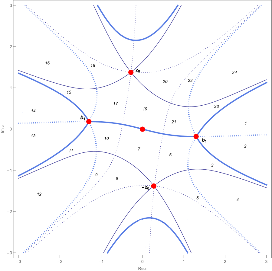
(a) The critical and critical orthogonal trajectories of the one-cut quadratic differential $Q_{1}(z;\sigma)\textrm{d}z^{2}$ incident with $\pm b_{1}$ and $\pm z_{0}$. Thick lines are associated with $\Re[\eta_{1}(z;\sigma)]=0$ (solid) and $\Im[\eta_{1}(z;\sigma)]=0$ (dotted), while the thin lines are associated with $\Re[\eta_{1,z_{0}}(z;\sigma)]=0$ (solid) and $\Im[\eta_{1,z_{0}}(z;\sigma)]=0$ (dotted), where we remind that $\eta_{1,e}(z;\sigma)=\int^{z}_{e}\sqrt{Q_{1}(s;\sigma)}\textrm{d}s$, and $\eta_{1}(z;\sigma)\equiv\eta_{1,b_{1}}(z;\sigma)$. The red dot which is not labeled represents the origin. We have only shown the "humps" $\mathcal{L}^{(1)}_{\sigma}$ and $\mathcal{L}^{(2)}_{\sigma}$ associated with $\Re[\eta_{1,b_{1}}(z;\sigma)]=0$ (See Lemma 3.12), and have not shown the humps associated with $\Im[\eta_{1,b_{1}}(z;\sigma)]=0$, $\Re[\eta_{1,z_{0}}(z;\sigma)]=0$, and $\Im[\eta_{1,z_{0}}(z;\sigma)]=0$ for simplicity of the Figure. Notice that $\eta_{1}(z;\sigma)\sim(z\mp b_{1})^{3/2}$ as $z\to\pm b_{1}$, while $\eta_{1}(z;\sigma)\sim(z\mp z_{0})^{2}$ as $z\to\pm z_{0}$, which determines the number of critical (critical orthogonal) trajectories incident with $\pm b_{1}$ and $\pm z_{0}$. The critical trajectories approach to infinity along the eight directions $\pi/8+k\pi/4$, and orthogonal trajectories approach to infinity along the eight directions $k\pi/4$, $k=0,\cdots,7$.

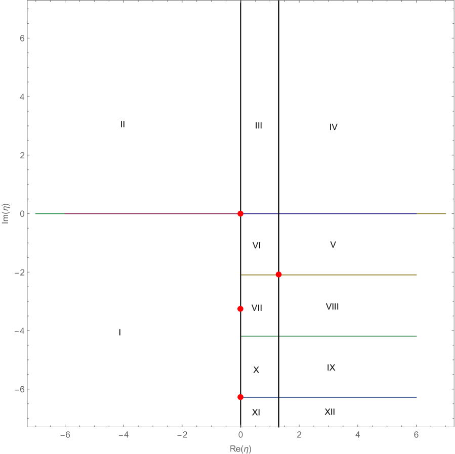
(b) The image $\eta_{1}(\Omega;\sigma)$, where $\Omega$ is the union of the regions labeled by $1$ through $12$ in Figure 2(a). Each strip-like region labeled by a Roman numeral corresponds to the region in Figure 2(a) labeled by the same number in Arabic numerals; for example the image of the region labeled by $6$ in Figure 2(a) is the region labeled by VI. Notice that $\eta_{1}(b_{1};\sigma)=0$, $\eta_{1,-}(0;\sigma)=-\pi\textrm{i}$, and $\eta_{1,-}(-b_{1};\sigma)=-2\pi\textrm{i}$, while the red point in the fourth quadrant represents $\eta_{1}(-z_{0};\sigma)$. The map $\eta$ is clearly not conformal at $\pm b_{1}$ and $\pm z_{0}$. For example a neighborhood of $b_{1}$ intersected with the regions labeled by 1, 2, 3, and 6 gets mapped to a full neighborhood of the origin in the $\eta$-plane due to $\eta_{1}(z;\sigma)\sim(z-b_{1})^{3/2}$ as $z\to b_{1}$, while a neighborhood of $-z_{0}$ intersected with the regions labeled by 5, 6, 7, and 8 gets mapped to a full neighborhood of $\eta_{1}(-z_{0};\sigma)$ in the $\eta$-plane due to $\eta_{1}(z;\sigma)\sim(z+z_{0})^{2}$ as $z\to-z_{0}$. The image $\eta_{1}(\Omega;\sigma)$ as depicted above shows that the regions in Figure 2(a) labeled by 1 and 2 are stable lands, meaning that they can host the complementary contours $\Gamma_{\sigma}[b_{1},\infty]$ and $\Gamma_{\sigma}[-\infty,-b_{1}]$, respectively.

Figure 2. Demonstration of the conformal mapping between the regions labeled by 1 through 12 in the $z$-plane to the $\eta_{1}$-plane. $\eta_{1}$ also maps the regions labeled by 13 to 24 to the entire plane as well. These conformal maps illustrate that the regions labeled by 1,2,13, and 14 are stable lands as shown in Figure 3(a). The stable lands in Figures 3(b) through 3(h) can be justified similarly.

Definition 3.8.

If $\Re\left[\eta_{1}(\pm z_{0}(\sigma);\sigma)\right]\neq 0$, we define $\Delta^{(b_{1})}$ (resp. $\Delta^{(-b_{1})}$) to be the geodesic polygon with vertices $b_{1}$ (resp. $-b_{1}$) and $\infty$, composed of $\ell_{2}^{(b_{1})}$ and $\ell_{3}^{(b_{1})}$ (resp. $\ell_{2}^{(-b_{1})}$ and $\ell_{3}^{(-b_{1})}$) with interior angle $2\pi/3$ at $b_{1}$ (resp. $-b_{1}$).

The following lemma is an immediate consequence of applying the Teichmüller’s lemma to the polygons $\Delta^{(\pm b_{1})}$.

Lemma 3.9.

The critical trajectories $\ell_{2}^{(b_{1})}$ and $\ell_{3}^{(b_{1})}$ approach to infinity along two directions $\pi/4$ apart if the geodesic polygon $\Delta^{(b_{1})}$ does not enclose $\pm z_{0}$, while they approach to infinity along two directions $3\pi/4$ apart if the geodesic polygon $\Delta^{(b_{1})}$ encloses one of $\pm z_{0}$. Due to symmetry the above statement is correct if we replace $b_{1}$ by $-b_{1}$.

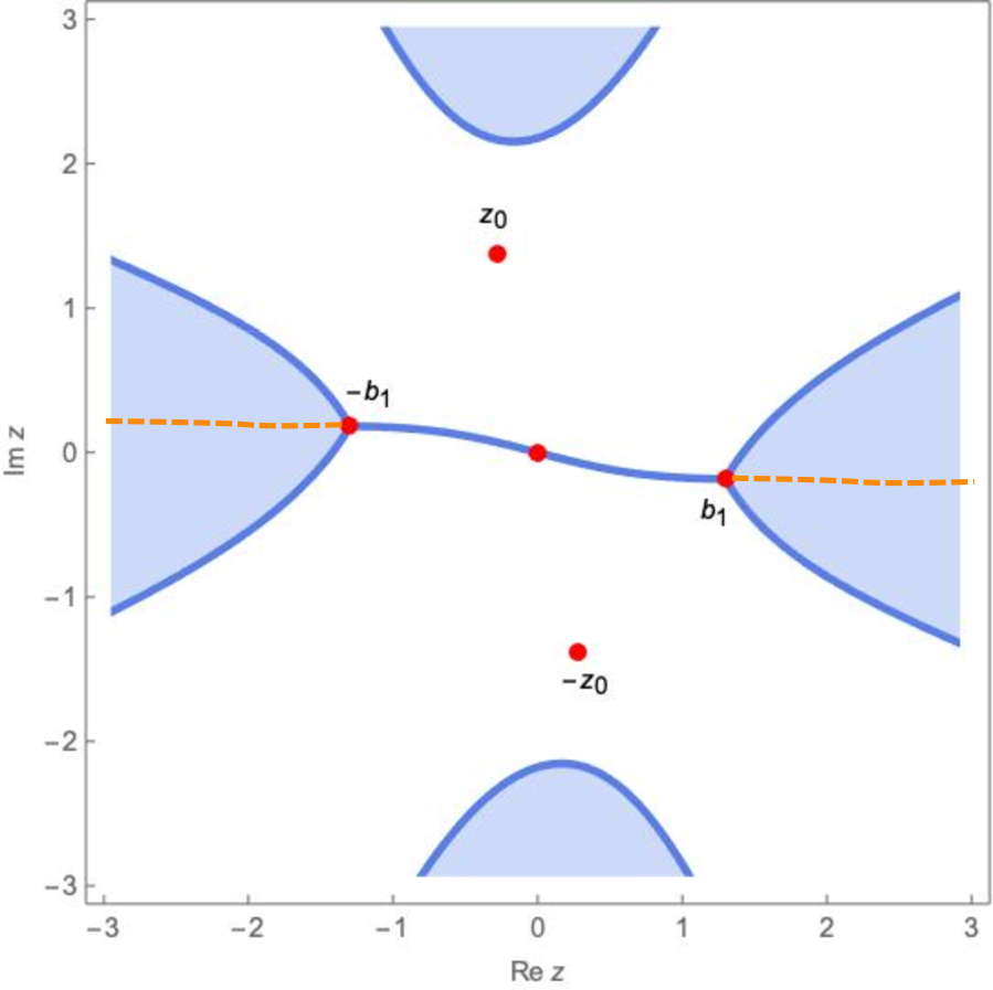
(a) $\sigma=1+\textrm{i}$.

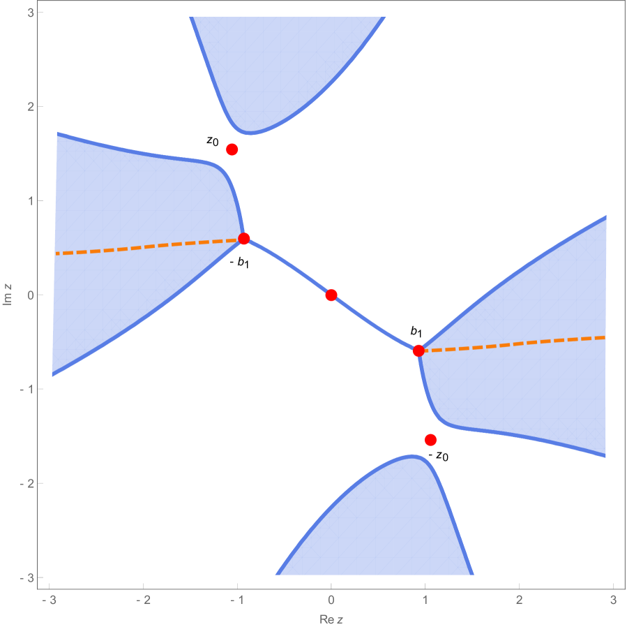
(b) $\sigma=1+3.8\textrm{i}$.

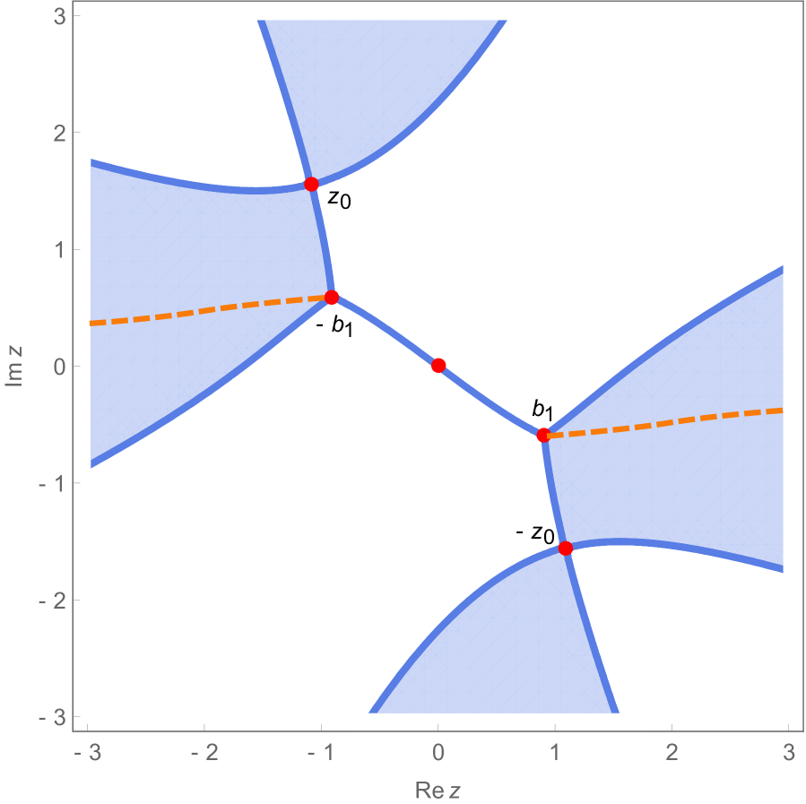
(c) $\sigma_{\mbox{cr}}\simeq 1+3.92\textrm{i}$.

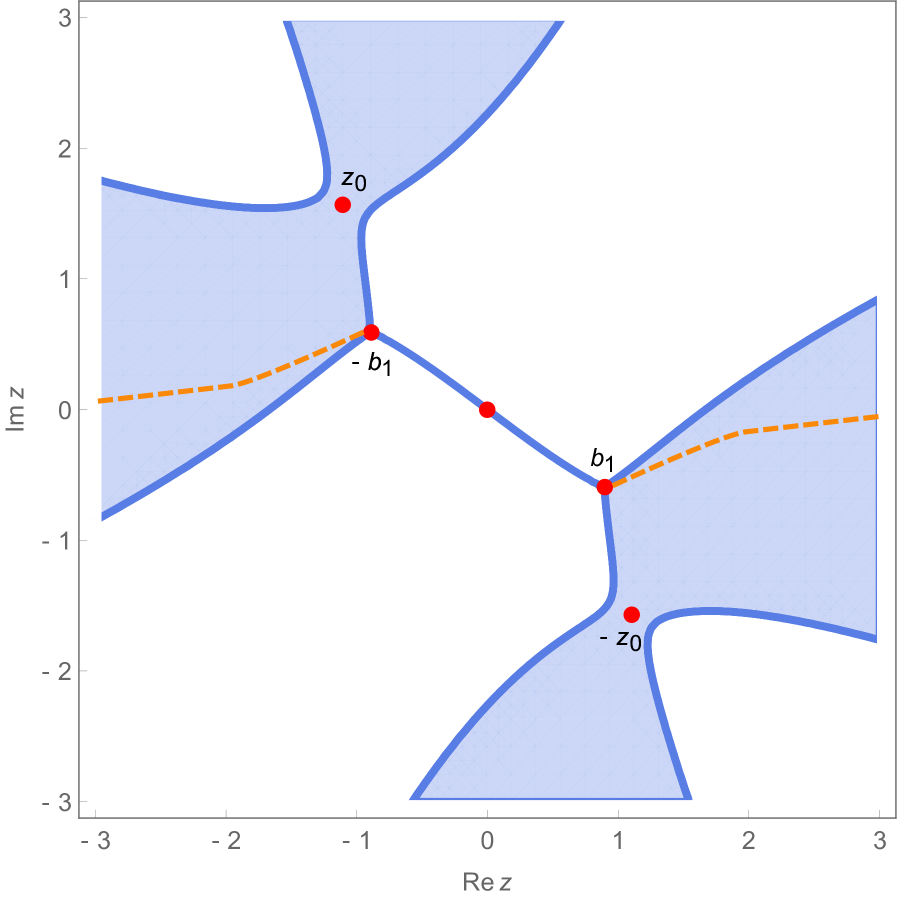
(d) $\sigma=1+4\textrm{i}$.

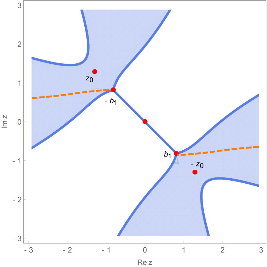
(e) $\sigma=4\textrm{i}$.

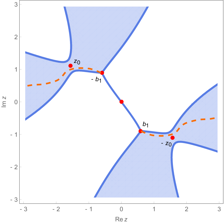
(f) $\sigma=-1+4\textrm{i}$.

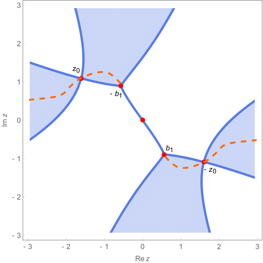
(g) $\sigma_{\mbox{cr}}\simeq-1.15+4\textrm{i}$.

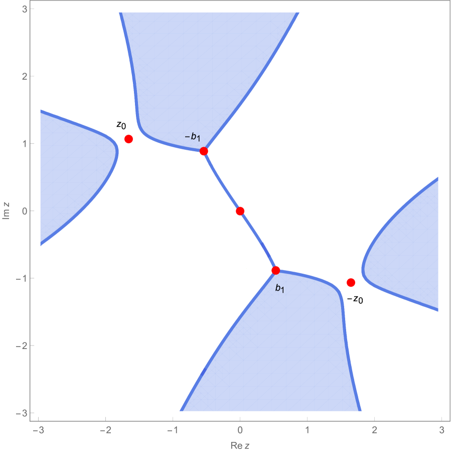
(h) $\sigma=-1.35+4\textrm{i}$.

Figure 3. This sequence of figures shows allowable regions in light blue through which the contour of integration (for the orthogonal polynomials) must pass, for a varying collection of values of $\sigma$. Regions in light blue are the $\sigma$-stable lands where $\Re[\eta_{1}(z;\sigma)]<0$ and the regions in white are the $\sigma$-unstable lands where $\Re[\eta_{1}(z;\sigma)]>0$. We denote the local critical arcs incident to $\pm b_{1}(\sigma)$ by $\mathcal{l}^{(\pm b_{1})}_{1}$, $\mathcal{l}^{(\pm b_{1})}_{2}$, and $\mathcal{l}^{(\pm b_{1})}_{3}$ (labeled in counterclockwise direction), where $\mathcal{l}^{(b_{1})}_{1}$ and $\mathcal{l}^{(-b_{1})}_{1}$ are the ones which are part of $J_{\sigma}\equiv\Gamma_{\sigma}[-b_{1},b_{1}]$. When $\pm z_{0}(\sigma)$ are in the $\sigma$-unstable lands, the Teichmüller’s lemma for the geodesic polygon comprised of $\ell^{(b_{1})}_{2}$ and $\ell^{(b_{1})}_{3}$ with vertices at $b_{1}(\sigma)$ and $\infty$, necessitates that $\ell^{(b_{1})}_{2}$ and $\ell^{(b_{1})}_{3}$ approach infinity along two directions $\pi/4$ radians apart (see Figures (a), (b) and (h) above), while when $\pm z_{0}(\sigma)$ are in the $\sigma$-stable lands, the Teichmüller’s lemma for the same geodesic polygon necessitates that $\ell^{(b_{1})}_{2}$ and $\ell^{(b_{1})}_{3}$ approach infinity along two directions $3\pi/4$ radians apart (see Figures (d), (e) and (f) above). In all figures above the first and the second requirements of Definition 3.1 is fulfilled. However, Figures (g) and (h) correspond to $\sigma$ values where the third requirement of Definition 3.1 is not met, while for $\sigma$ values corresponding to Figures (a) through (f), the orange dashed lines show that this requirement is fulfilled. In Figure 14(b) we show the location of these points with respect to the critical lines in the $\sigma$-plane.

Definition 3.10.

The subset $\mathcal{O}^{*}_{1}$ in the $\sigma$-plane is the collection of all $\sigma\in{\mathbb{C}}$ such that

1. The critical graph $\mathscr{J}^{(1)}_{\sigma}$ of all points $z$ satisfying

   (3.11) $$\Re\left[\eta_{1}(z;\sigma)\right]=0,$$

   contains a single Jordan arc $J_{\sigma}$ connecting $-b_{1}(\sigma)$ to $b_{1}(\sigma)$,

2. The points $\pm z_{0}(\sigma)$ do not lie on $\mathscr{J}^{(1)}_{\sigma}$, and

3. There exists a complementary arc $\Gamma_{\sigma}(b_{1}(\sigma),\infty)$ which lies entirely in the component of the set

   (3.12) $$\left\{z:\Re\left[\eta_{1}(z;\sigma)\right]<0\right\},$$

   which encompasses $(M(\sigma),\infty)$ for some $M(\sigma)>0$.

Notice that $\mathcal{O}^{*}_{1}\subseteq\mathcal{O}_{1}$, since for the definition of $\mathcal{O}^{*}_{1}$ the location of $z_{0}$ is further restricted than what is required for the definition of $\mathcal{O}_{1}$. In Theorem 4.5 the significance of distinguishing these two sets will become more clear. Here in the rest of this section we will focus on proving the following Theorem:

Theorem 3.11.

The set $\mathcal{O}^{*}_{1}$ is open.

We prove this Theorem by proving several lemmas associated to the different requirements of Definition 3.10. In the following three lemmas we establish some structural properties of the critical graph $\mathscr{J}^{(1)}_{\sigma}$.

Lemma 3.12.

Suppose that $\sigma\in\mathcal{O}^{*}_{1}$ and $\Re[\eta_{1}(\pm z_{0}(\sigma);\sigma)]>0$. Then there exist two disjoint curves $\mathcal{L}^{(1)}_{\sigma}$ and $\mathcal{L}^{(2)}_{\sigma}$ as subsets of $\mathscr{J}^{(1)}_{\sigma}$, which have no intersections with $\pm b_{1}(\sigma)$, $\pm z_{0}(\sigma)$, $J_{\sigma}$, $\ell_{2}^{(b_{1})},\ell_{3}^{(b_{1})},\ell_{2}^{(-b_{1})}$, and $\ell_{3}^{(-b_{1})}$. Moreover, the curve $\mathcal{L}^{(1)}_{\sigma}$ approaches to infinity along the two directions $3\pi/8$ and $5\pi/8$, the curve $\mathcal{L}^{(2)}_{\sigma}$ approaches to infinity along the two directions $-3\pi/8$ and $-5\pi/8$, and the rays $\ell_{2}^{(b_{1})},\ell_{3}^{(b_{1})},\ell_{2}^{(-b_{1})}$, and $\ell_{3}^{(-b_{1})}$ respectively approach to infinity along the directions $-\pi/8$, $\pi/8$, $7\pi/8$, and $-7\pi/8$.

Proof.

Since $\Re[\eta_{1}(\pm z_{0}(\sigma);\sigma)]\neq 0$, all four rays $\ell_{2}^{(b_{1})},\ell_{3}^{(b_{1})},\ell_{2}^{(-b_{1})}$, and $\ell_{3}^{(-b_{1})}$ must extend off to infinity according to Lemma 3.7. By a conformal mapping argument, one can easily confirm that in a neighborhood $\mathscr{O}$ of $b_{1}(\sigma)$, for all $z\in\mathscr{O}\cap\Delta^{(b_{1})}$ we have $\Re[\eta_{1}(z;\sigma)]<0$. Since $\sigma\in\mathcal{O}^{*}_{1}$, some ray $\Gamma_{\sigma}(b_{1}(\sigma),\infty)$ must start from $b_{1}(\sigma)$ within the subset $\mathscr{O}\cap\Delta^{(b_{1})}$ and stay within $\Delta^{(b_{1})}$ (intersection of $\Gamma_{\sigma}(b_{1}(\sigma),\infty)$ with boundaries of $\Delta^{(b_{1})}$ is not possible since on $\Gamma_{\sigma}(b_{1}(\sigma),\infty)$ we have $\Re[\eta_{1}(z;\sigma)]<0$ while on the boundaries of $\Delta^{(b_{1})}$ we have $\Re[\eta_{1}(z;\sigma)]=0$).

Now, we show that the interior of $\Delta^{(b_{1})}$ does not contain $\pm z_{0}(\sigma)$. It suffices to prove that the sign of $\Re[\eta_{1}(z;\sigma)]$ does not change in the interior of $\Delta^{(b_{1})}$, because if so, then for all $z$ in the interior of $\Delta^{(b_{1})}$ we would have $\Re[\eta_{1}(z;\sigma)]<0$, while it is assumed that $\Re[\eta_{1}(\pm z_{0}(\sigma);\sigma)]>0$. Notice that due to continuity, the sign of $\Re[\eta_{1}(z;\sigma)]$ could only change in the interior of $\Delta^{(b_{1})}$ if there is a curve $\mathcal{L}$ separating the regions where $\Re[\eta_{1}(z;\sigma)]<0$ and $\Re[\eta_{1}(z;\sigma)]>0$ with the following properties: $\mathcal{L}$ is a solution of $\Re[\eta_{1}(z;\sigma)]=0$, lies within $\Delta^{(b_{1})}$ and not intersecting its boundaries $\ell_{2}^{(b_{1})}$ and $\ell_{3}^{(b_{1})}$. Being a critical trajectory, the curve $\mathcal{L}$ must go off to infinity. In the region circumscribed by $\mathcal{L}$ and the boundaries of $\Delta^{(b_{1})}$ we have $\Re[\eta_{1}(z;\sigma)]<0$ so it can not contain $\pm z_{0}(\sigma)$. The interior of $\mathcal{L}$ (where $\Re[\eta_{1}(z;\sigma)]>0$) can not contain $z_{0}(\sigma)$ either, since if it does, $\mathcal{L}$ has to approach to infinity along two directions $3\pi/4$ radians apart by Teichmüller’s lemma, which then means that the boundaries of $\Delta^{(b_{1})}$ must approach to infinity along two directions $5\pi/4$ radians apart. But this is a contradiction, since the symmetry relation (3.7) would imply that there has to be intersections between the boundaries of $\Delta^{(b_{1})}$ and $\Delta^{(-b_{1})}$, which is not possible as the only singular points for the quadratic differential (3.8) are $\pm b_{1}(\sigma)$ and $\pm z_{0}(\sigma)$. This finishes the proof that the interior of $\Delta^{(b_{1})}$ does not contain $\pm z_{0}(\sigma)$.

Now it is clear that $\ell_{2}^{(b_{1})}$ and $\ell_{3}^{(b_{1})}$ must approach to infinity along the directions $-\pi/8$ and $\pi/8$ respectively, as any other choice either: a) does not allow $\Delta^{(b_{1})}$ to encompass $(M(\sigma),\infty)$ for some $M(\sigma)>0$, or b) violates Lemma 3.9. By the symmetry relation (3.7) we immediately conclude that $\ell_{2}^{(-b_{1})}$, and $\ell_{3}^{(-b_{1})}$ respectively approach to infinity along the directions $7\pi/8$, and $-7\pi/8$.

These rays provide four solutions at infinity. Since there are eight solutions at infinty, the other four solutions must come from two curves $\mathcal{L}^{(1)}_{\sigma}$ and $\mathcal{L}^{(2)}_{\sigma}$ each pointing towards infinity in two directions $\pi/4$ radians apart. Each of these curves do approach to infinity along two directions as they can not be incident with $\pm z_{0}(\sigma)$ or $\pm b_{1}(\sigma)$. The curves $\mathcal{L}^{(1)}_{\sigma}$ and $\mathcal{L}^{(2)}_{\sigma}$ must be symmetric with respect to the origin due to (3.7). We denote the one in the upper-half plane by $\mathcal{L}^{(1)}_{\sigma}$ and the one in the lower-half plane by $\mathcal{L}^{(2)}_{\sigma}$. From what we proved earlier about the rays $\ell_{2}^{(b_{1})},\ell_{3}^{(b_{1})},\ell_{2}^{(-b_{1})}$, and $\ell_{3}^{(-b_{1})}$, it is now clear that the curve $\mathcal{L}^{(1)}_{\sigma}$ approaches to infinity along the two directions $3\pi/8$ and $5\pi/8$, the curve $\mathcal{L}^{(2)}_{\sigma}$ approaches to infinity along the two directions $-3\pi/8$ and $-5\pi/8$. ∎

The following lemmas can be proven using identical arguments and thus we only state the result (see Figure 3(d)).

Lemma 3.13.

Suppose that $\sigma\in\mathcal{O}^{*}_{1}$, $\Re[\eta_{1}(\pm z_{0}(\sigma);\sigma)]<0$, and $\Re[z_{0}(\sigma)]<0$. Then there exist two disjoint curves $\mathcal{L}^{(3)}_{\sigma}$ and $\mathcal{L}^{(4)}_{\sigma}$ as subsets of $\mathscr{J}^{(1)}_{\sigma}$, which have no intersections with $\pm b_{1}(\sigma)$, $\pm z_{0}(\sigma)$, $J_{\sigma}$, $\ell_{2}^{(b_{1})},\ell_{3}^{(b_{1})},\ell_{2}^{(-b_{1})}$, and $\ell_{3}^{(-b_{1})}$. Moreover, the curve $\mathcal{L}^{(3)}_{\sigma}$ approaches to infinity along the two directions $5\pi/8$ and $7\pi/8$, the curve $\mathcal{L}^{(4)}_{\sigma}$ approaches to infinity along the two directions $-3\pi/8$ and $-\pi/8$, and the rays $\ell_{2}^{(b_{1})},\ell_{3}^{(b_{1})},\ell_{2}^{(-b_{1})}$, and $\ell_{3}^{(-b_{1})}$ respectively approach to infinity along the directions $-5\pi/8$, $\pi/8$, $3\pi/8$, and $-7\pi/8$.

Lemma 3.14.

Suppose that $\sigma\in\mathcal{O}^{*}_{1}$, $\Re[\eta_{1}(\pm z_{0}(\sigma);\sigma)]<0$, and $\Re[z_{0}(\sigma)]>0$. Then there exist two disjoint curves $\mathcal{L}^{(5)}_{\sigma}$ and $\mathcal{L}^{(6)}_{\sigma}$ as subsets of $\mathscr{J}^{(1)}_{\sigma}$, which have no intersections with $\pm b_{1}(\sigma)$, $\pm z_{0}(\sigma)$, $J_{\sigma}$, $\ell_{2}^{(b_{1})},\ell_{3}^{(b_{1})},\ell_{2}^{(-b_{1})}$, and $\ell_{3}^{(-b_{1})}$. Moreover, the curve $\mathcal{L}^{(5)}_{\sigma}$ approaches to infinity along the two directions $\pi/8$ and $3\pi/8$, the curve $\mathcal{L}^{(6)}_{\sigma}$ approaches to infinity along the two directions $-5\pi/8$ and $-7\pi/8$, and the rays $\ell_{2}^{(b_{1})},\ell_{3}^{(b_{1})},\ell_{2}^{(-b_{1})}$, and $\ell_{3}^{(-b_{1})}$ respectively approach to infinity along the directions $-\pi/8$, $5\pi/8$, $7\pi/8$, and $-3\pi/8$.

Lemma 3.15.

When $z_{0}(\sigma)\in\mathscr{J}^{(1)}_{\sigma}$, the components $\mathcal{L}^{(j)}_{\sigma}$ and $\mathcal{L}^{(j+1)}_{\sigma}$, $j=1,3,5$ (respectively for the curves defined in Lemmas 3.12, 3.13, and 3.14), are connected to the rest of the critical graph at $\pm z_{0}$.

Proof.

This is the only possibility, as if $\mathcal{L}^{(j)}_{\sigma}$ and $\mathcal{L}^{(j+1)}_{\sigma}$ are not connected to the rest of the critical graph at $\pm z_{0}$, one would have too many (more than $8$) solutions of the equation $\Re[\eta_{1}(z;\sigma)]=0$ at $\infty$. ∎

Lemma 3.16.

Any $\sigma>-2$ belongs to $\mathcal{O}^{*}_{1}$ and $\pm z_{0}(\sigma)$ belong to unstable lands.

Proof.

For $\sigma>-2$, we know that $b_{1}>0$ and $z_{0}=\textrm{i}y_{0}$, with $y_{0}>0$. The local structure of the critical trajectories in a neighborhood of the critical points can be easily found by finding a ray on which $Q_{1}(z;\sigma)\textrm{d}z^{2}<0$. Locally, the other critical trajectories will be then determined based on how many critical directions are incident with the critical point. It is clear that the real interval $(-b_{1},b_{1})$ must be a short critical trajectory, because it is incident with $\pm b_{1}$, $Q_{1}(z;\sigma)<0$ for all $z\in(-b_{1},b_{1})$, and $\textrm{d}z^{2}>0$ for all infinitesimal real line segments $\textrm{d}z$. Using the explicit formula (4.1) one can show that $\Re[\eta_{1}(z_{0}(\sigma);\sigma)]>0$ for all $\sigma>-2$. Using (3.7), we immediately have $\Re\left[\eta_{1}\left(-z_{0}(\sigma);\sigma\right)\right]>0$ for all $\sigma>-2$, as well. So far we have shown that all $\sigma>-2$ satisfy the first two requirements of Definition 3.10. Now, we prove that the third requirement is met as well. Notice that, for fixed $\sigma>-2$, the function $\eta_{1}(x;\sigma)$ is real and negative for all $x>b_{1}(\sigma)$. This means that the complementary arc $\Gamma_{\sigma}(b_{1}(\sigma),\infty)$ in the third requirements of Definition 3.10, can be chosen as the real interval $(b_{1}(\sigma);\infty)$ for $\sigma>-2$.

∎

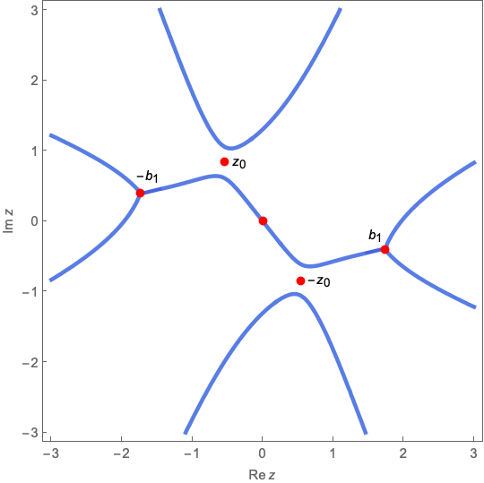
(a) The critical graph $\mathscr{J}^{(1)}_{\sigma}$ when there is a connection from $-b_{1}$ to $b_{1}$.

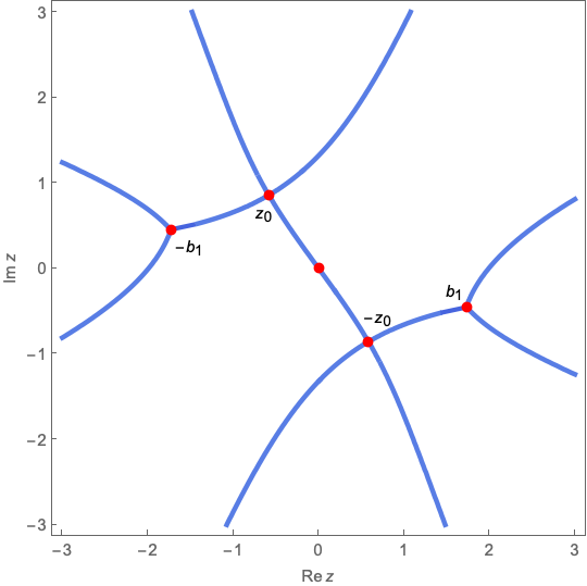
(b) The critical graph $\mathscr{J}^{(1)}_{\sigma}$ at a critical value $\sigma_{*}$ (See Lemma 3.18).

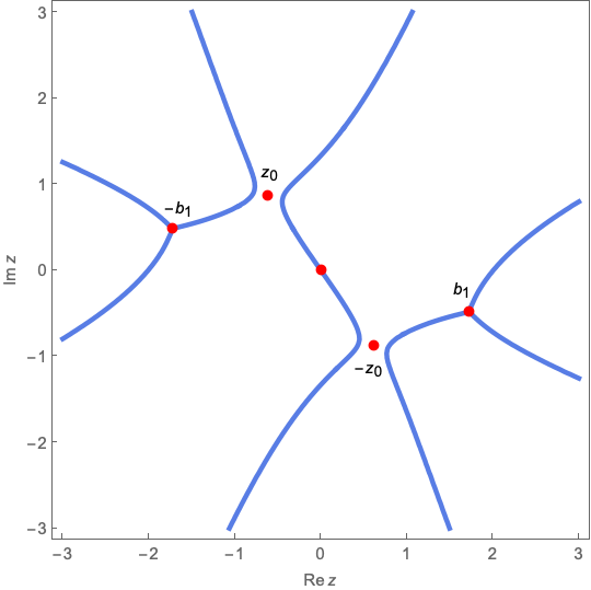
(c) The critical graph $\mathscr{J}^{(1)}_{\sigma}$ when there is no connection from $-b_{1}$ to $b_{1}$.

Figure 4. Schematic of the continuous deformation of the critical graph $\mathscr{J}^{(1)}_{\sigma}$ ( the collection of all points $z$ satisfying $\Re\left[\eta_{1}(z;\sigma)\right]=0$ ) from a $\sigma\in\mathcal{O}^{*}_{1}$ where there is a connection from $-b_{1}$ to $b_{1}$, to a $\sigma\notin\mathcal{O}^{*}_{1}$ where $-z_{0}$ and $z_{0}$ both lie on $\mathscr{J}^{(1)}_{\sigma}$, and finally to a $\sigma\notin\mathcal{O}^{*}_{1}$ where there is no connection from $-b_{1}$ to $b_{1}$.

Lemma 3.17.

Let $\sigma_{0}\in\mathcal{O}^{*}_{1}$ and not on the branch cuts of $\Re[\eta_{1}(z_{0}(\sigma);\sigma)]$. Then there exists $\delta>0$, such that for all $\sigma$ in the $\delta$-neighborhood $\{\sigma:|\sigma-\sigma_{0}|<\delta\}$ of $\sigma_{0}$, the points $\pm z_{0}(\sigma)$ do not lie on $\mathscr{J}^{(1)}_{\sigma}$.

Proof.

Since $\sigma_{0}\in\mathcal{O}^{*}_{1}$ we have $\Re[\eta_{1}(z_{0}(\sigma_{0});\sigma_{0})]\neq 0$, so without loss of generality assume that $\Re[\eta_{1}(z_{0}(\sigma_{0});\sigma_{0})]>0$. Since the function $\Re[\eta_{1}(z_{0}(\sigma);\sigma)]$ is continuous at $\sigma_{0}$, there exists $\delta>0$, such that the sign of $\Re[\eta_{1}(z_{0}(\sigma);\sigma)]$ is the same as sign of $\Re[\eta_{1}(z_{0}(\sigma_{0});\sigma_{0})]$ for all $\sigma$ in the $\delta$-neighborhood $\{\sigma:|\sigma-\sigma_{0}|<\delta\}$ of $\sigma_{0}$. ∎

Lemma 3.18.

Let $\sigma_{0}$ and $\delta$ have the same meaning as in Lemma 3.17. For any $\hat{\sigma}$ in the $\delta$-neighborhood of $\sigma_{0}$, there is still a connection from $-b_{1}(\hat{\sigma})$ to $b_{1}(\hat{\sigma})$ and therefore there still exist two disjoint curves $\mathcal{L}^{(1)}_{\hat{\sigma}}$ and $\mathcal{L}^{(2)}_{\hat{\sigma}}$ as subsets of $\mathscr{J}^{(1)}_{\hat{\sigma}}$ with the same description as given in Lemma 3.12, Lemma 3.13, or Lemma 3.14.

Proof.

Assume that, at $\hat{\sigma}$ there is no longer a connection from $-b_{1}(\hat{\sigma})$ to $b_{1}(\hat{\sigma})$. Therefore all six rays $\ell_{1}^{(b_{1}(\hat{\sigma}))}$,$\ell_{2}^{(b_{1}(\hat{\sigma}))},$ $\ell_{3}^{(b_{1}(\hat{\sigma}))},$ $\ell_{1}^{(-b_{1}(\hat{\sigma}))},$ $\ell_{2}^{(-b_{1}(\hat{\sigma}))},$ $\ell_{3}^{(-b_{1}(\hat{\sigma}))}$ must extend to infinity since none can be connected to either $z_{0}(\hat{\sigma})$ or $-z_{0}(\hat{\sigma})$ by the choice of $\delta$. The other two solutions at infinity must come from a curve $\mathcal{L}$ symmetric with respect to the origin. Since we have four finite singular points, $\mathcal{L}$ must have one singular point of order 2 ($z_{0}(\hat{\sigma})$ or $-z_{0}(\hat{\sigma})$) and one singular point of order one ($b_{1}(\hat{\sigma})$ or $-b_{1}(\hat{\sigma})$) on one side, and the other pair of singular points on the other side. By Teichmüller’s lemma this curve approaches to infinity along two rays $\pi$ radians apart as shown in Figure 4(c).

Consider a path $\gamma:[0,1]\to\{\sigma:|\sigma-\sigma_{0}|<\delta\}$, with $\gamma(0)=\sigma_{0}$ and $\gamma(1)=\hat{\sigma}$. Since the level sets $\mathscr{J}^{(1)}_{\sigma}$ deform in a continuous fashion with respect to $\sigma$ (for a schematic of three snapshots of this deformation see Figure 4), the above scenario requires existence of a value $\sigma_{*}=\gamma(t_{*})$ for some $0<t_{*}<1$ such that $z_{0}(\sigma_{*})\in\mathscr{J}^{(1)}_{\sigma_{*}}$. But this is impossible by the choice of $\delta$ in Lemma 3.17, as it would mean $\Re[\eta_{1}(z_{0}(\sigma_{*}),\sigma_{*})]=0$. ∎

Lemma 3.19.

Let $\sigma_{0}$ and $\delta$ have the same meaning as in Lemma 3.17. Then for all $\sigma$ in the $\delta$-neighborhood of $\sigma_{0}$, there exists a complementary arc $\Gamma_{\sigma}(b_{1}(\sigma),\infty)$ which lies entirely in the component of the set

(3.13) $$\left\{z:\Re\left[\eta_{1}(z;\sigma)\right]<0\right\},$$

which encompasses $(M(\sigma),\infty)$ for some $M(\sigma)>0$.

Proof.

The structure of critical trajectories does not change unless $z_{0}(\sigma)$ hits the set $\mathscr{J}^{(1)}_{\sigma}$. By the choice of $\delta$ and $\sigma_{0}$, this does not happen for any $\sigma$ in the $\delta$-neighborhood of $\sigma_{0}$. ∎

Lemmas 3.17, 3.18, and 3.19 are together equivalent to Theorem 3.11.

3.2. The Two-cut Regime.

Let us recall from §2.4.2 that the quadratic differential for the two cut regime is

(3.14) $$Q_{2}(z;\sigma)\textrm{d}z^{2}:=z^{2}\left(z^{2}-a^{2}_{2}(\sigma)\right)\left(z^{2}-b^{2}_{2}(\sigma)\right)\textrm{d}z^{2}.$$

From (2.60) we recall that $a_{2}\neq b_{2}$ and $a_{2},b_{2}\neq 0$ away from $\sigma=\pm 2$. Identical to the one-cut quadratic differential (3.8), we can show that the solutions to $\Re[\eta_{2}(z;\sigma)]$ approach to infinity along the eight directions

$$\{\pi/8+k\pi/4:k=0,\cdots,7\}.$$

Lemma 3.20.

There are no singular finite geodesic polygons with one or two vertices associated to the quadratic differential (3.14).

Proof.

The proof is identical to the proof of Lemma 3.5. ∎

Definition 3.21.

Define the subset $\mathcal{O}_{2}$ in the $\sigma$-plane as the collection of all $\sigma\in{\mathbb{C}}$ such that

1. The critical graph $\mathscr{J}^{(2)}_{\sigma}$ of all points $z$ satisfying

   (3.15) $$\Re\left[\eta_{2}(z;\sigma)\right]=0,$$

   contains a single Jordan arc connecting $-b_{2}(\sigma)$ to $-a_{2}(\sigma)$ and a single Jordan arc connecting $a_{2}(\sigma)$ to $b_{2}(\sigma)$,

2. There exists a complementary arc $\Gamma_{\sigma}(b_{2}(\sigma),\infty)$ which lies entirely in the component of the set

   (3.16) $$\left\{z:\Re\left[\eta_{2}(z;\sigma)\right]<0\right\},$$

   which encompasses $(M(\sigma),\infty)$ for some $M(\sigma)>0$,

3. There exists a complementary arc $\Gamma_{\sigma}(-a_{2}(\sigma),a_{2}(\sigma))$ which lies entirely in the component of the set

   (3.17) $$\left\{z:\Re\left[\eta_{2}(z;\sigma)\right]<0\right\}.$$

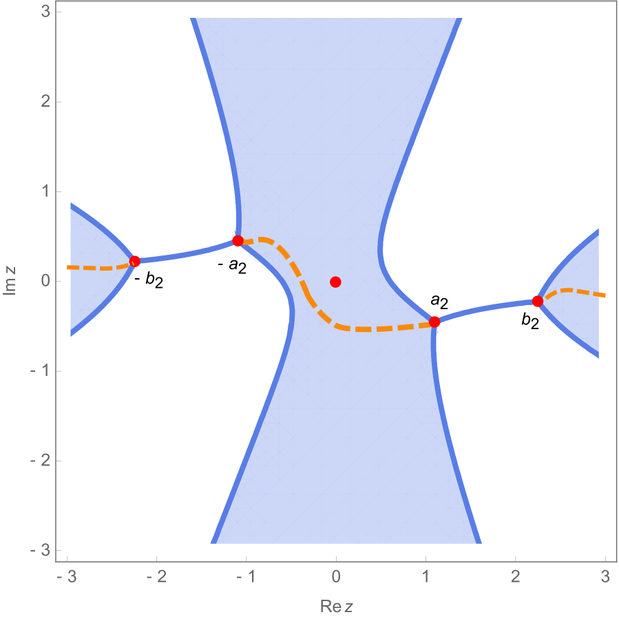
(a) $\sigma=-3+\textrm{i}$.

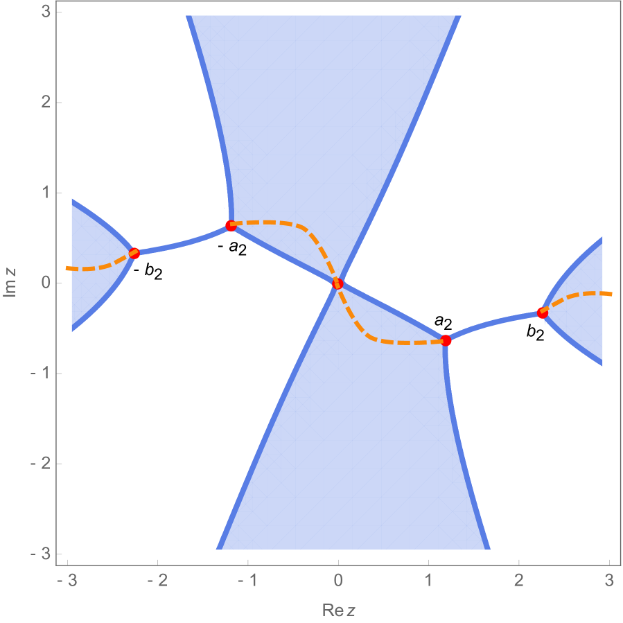
(b) $\sigma_{\mbox{cr}}\simeq-3+1.5\textrm{i}$.

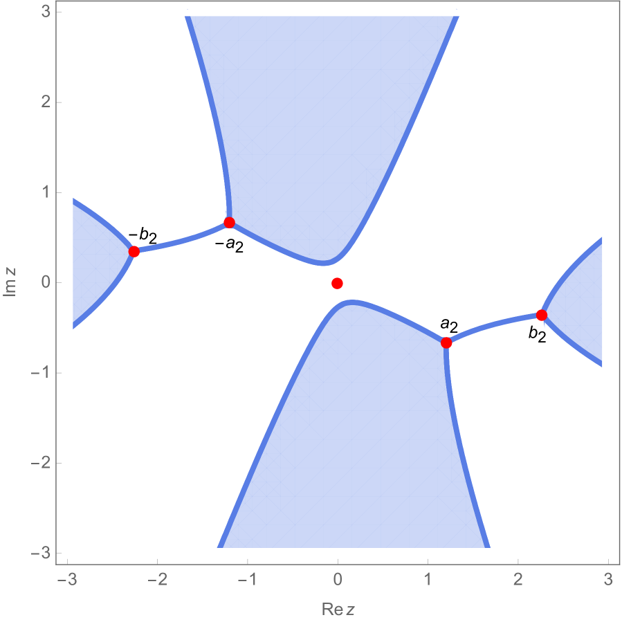
(c) $\sigma=-3+1.6\textrm{i}$.

Figure 5. This sequence of figures shows allowable regions in light blue through which the contour of integration (for the orthogonal polynomials) must pass, for a varying collection of values of $\sigma$. Regions in light blue are the $\sigma$-stable lands where $\Re[\eta_{2}(z;\sigma)]<0$ and the regions in white are the $\sigma$-unstable lands where $\Re[\eta_{2}(z;\sigma)]>0$. Figure (a) corresponds to a $\sigma\in\mathcal{O}_{2}$ as all conditions of Definition 3.21 are satisfied. Figures (b) and (c) do not correspond to $\sigma\in\mathcal{O}_{2}$, as the third requirement of the definition 3.21 is not satisfied.

Theorem 3.22.

The set $\mathcal{O}_{2}$ as defined in Definition 3.21 is open.

The following Lemmas, collectively, establish the above Theorem.

Lemma 3.23.

The set $\mathscr{J}^{(2)}_{\sigma}$ is symmetric with respect to the origin.

Proof.

In view of the first part of Definition 3.21, this simply follows from the identity

(3.18) $$\eta_{2}(-z;\sigma)=\eta_{2}(z;\sigma)\pm 2\pi\textrm{i}.$$

∎

Lemma 3.24.

[Theorem 3 of [BBG⁺22]] The critical graph $\mathscr{J}^{(2)}_{\sigma}$ deforms continuously with respect to $\sigma$.

Lemma 3.25.

If $0\in\mathscr{J}^{(2)}_{\sigma}$, either $\ell^{(a_{2})}_{2}$ must connect to $\ell^{(-a_{2})}_{2}$, or $\ell^{(a_{2})}_{3}$ must connect to $\ell^{(-a_{2})}_{3}$ at the origin.

Proof.

This is necessary due to symmetry and to avoid too many (more than $8$) solutions of the equation $\Re[\eta_{2}(z;\sigma)]=0$ at $\infty$. ∎

Corollary 3.25.1.

If for some $\sigma$ we have $0\in\mathscr{J}^{(2)}_{\sigma}$, then $\sigma\notin\mathcal{O}_{2}$.

Proof.

This is obvious now from the previous Lemma, since any path $\Gamma_{\sigma}(-a_{2},a_{2})$ can not entirely lie in $\left\{z:\Re\left[\eta_{2}(z;\sigma)\right]<0\right\}$ as $\mathscr{J}^{(2)}_{\sigma}$ has formed a barrier between $-a_{2}$ and $a_{2}$ (See Figure 5(b)). ∎

Lemma 3.26.

Any $\sigma<-2$ belongs to $\mathcal{O}_{2}$.

Proof.

This can be proven in an identical way as Lemma 3.16 and we do not provide the details here. ∎

Lemma 3.27.

Let $\sigma_{0}\in\mathcal{O}_{2}$ and not on the branch cuts of $\Re[\eta_{2}(0;\sigma)]$. Then there exists $\delta>0$, such that for all $\sigma$ in the $\delta$-neighborhood $\{\sigma:|\sigma-\sigma_{0}|<\delta\}$ of $\sigma_{0}$, the point at the origin does not lie on $\mathscr{J}^{(2)}_{\sigma}$.

Proof.

Since $\sigma_{0}\in\mathcal{O}_{2}$ we have $\Re[\eta_{2}(0;\sigma_{0})]\neq 0$. Since the function $\Re[\eta_{2}(0;\sigma)]$ is continuous at $\sigma_{0}$, there exists $\delta>0$, such that the sign of $\Re[\eta_{2}(0;\sigma)]$ is the same as sign of $\Re[\eta_{2}(0;\sigma_{0})]$ for all $\sigma$ in the $\delta$-neighborhood $\{\sigma:|\sigma-\sigma_{0}|<\delta\}$ of $\sigma_{0}$. ∎

The points $\pm a_{2}$ and $\pm b_{2}$ are all simple zeros of the quadratic differential. So three critical trajectories emanate from each one. We denote the local critical arcs incident to $p$ by $\ell^{(p)}_{1}$, $\ell^{(p)}_{2}$, $\ell^{(p)}_{3}$ (labeled in counterclockwise direction), where $\ell^{(p)}_{1}$ is the critical arc emanating from $p$ which makes the connection prescribed in the first requirement of Definition 3.21, $p=\pm a_{2},\pm b_{2}$.

Lemma 3.28.

Let $\sigma\in\mathcal{O}_{2}$. The critical arcs $\ell_{2}^{(-b_{2})}$, $\ell_{3}^{(-b_{2})}$, $\ell_{2}^{(-a_{2})}$, $\ell_{3}^{(-a_{2})}$,$\ell_{2}^{(a_{2})}$, $\ell_{3}^{(a_{2})}$,$\ell_{2}^{(b_{2})}$, and $\ell_{3}^{(b_{2})}$, respectively approach to infinity along the directions $7\pi/8$, $-7\pi/8$, $-5\pi/8$, $5\pi/8$, $3\pi/8$, $-3\pi/8$, $-\pi/8$, and $\pi/8$. Moreover, the $\sigma$-stable and $\sigma$-unstable lands having these critical arcs as boundaries are as given in Figure 5(a), and in particular, $\Re[\eta_{2}(0;\sigma)]<0$.

Proof.

It is easy to verify that no two critical arcs from the set $\bm{L}:=\{\ell^{(p)}_{2},\ell^{(p)}_{3}:p=\pm a_{2},\pm b_{2}\}$, can be connected to one another, as it would violate Lemma 3.20, or would lead to geodesic polygons with more than two vertices which are not allowed by Teichmüller’s Lemma. Moreover, no critical arc from the set $\bm{L}$ can be connected to the origin due to the third requirement of the Definition 3.21. Therefore all critical arcs from the set $\bm{L}$ must approach infinity.

Notice that the point at the origin can not be enclosed by the geodesic polygon with vertices $b_{2}$ and $\infty$ defined by $\ell_{2}^{(b_{2})}$, $\ell_{3}^{(b_{2})}$. This is because, due to the symmetry of the critical graph with respect to the origin, $\ell_{2}^{(b_{2})}$ and $\ell_{3}^{(b_{2})}$ are respectively reflections of $\ell_{2}^{(-b_{2})}$ and $\ell_{3}^{(-b_{2})}$ through the origin. So if the the geodesic polygon with vertices $b_{2}$ and $\infty$ defined by $\ell_{2}^{(b_{2})}$, $\ell_{3}^{(b_{2})}$ encloses the origin, so does the geodesic polygon with vertices $-b_{2}$ and $\infty$ defined by $\ell_{2}^{(-b_{2})}$, $\ell_{3}^{(-b_{2})}$. But this would mean that there is an intersection between at least one ray emanating from $b_{2}$ and one ray emanating from $-b_{2}$ at a regular point, which is impossible. For a similar reason, one can show that the endpoints $-b_{2},-a_{2}$ and $a_{2}$ can not be enclosed by the geodesic polygon with vertices $b_{2}$ and $\infty$ defined by $\ell_{2}^{(b_{2})}$, $\ell_{3}^{(b_{2})}$. Now the Teichmüller’s Lemma implies that the critical rays $\ell_{2}^{(b_{2})}$ and $\ell_{3}^{(b_{2})}$ must approach $\infty$ along two directions $\pi/4$ radians apart. Therefore, in order to satisfy the third requirement of the Definition 3.21, $\ell_{2}^{(b_{2})}$ and $\ell_{3}^{(b_{2})}$ must respectively approach to $-\pi/8$, and $\pi/8$.

Now, we notice that the geodesic polygon with three vertices $a_{2},b_{2}$, and $\infty$, comprised of $\ell^{(b_{2})}_{1},\ell^{(b_{2})}_{3}$, and $\ell^{(a_{2})}_{2}$ can not enclose the origin, because in that case, by symmetry it would enforce the geodesic polygon with three vertices $-a_{2},-b_{2}$, and $\infty$, comprised of $\ell^{(-b_{2})}_{1},\ell^{(-b_{2})}_{3}$, and $\ell^{(-a_{2})}_{2}$ also enclose the origin, which then implies the failure of the fourth requirement of the Definition 3.21 (See Figure 5(c)). The same argument shows that the geodesic polygon with three vertices $a_{2},b_{2}$, and $\infty$, comprised of $\ell^{(b_{2})}_{1},\ell^{(b_{2})}_{2}$, and $\ell^{(a_{2})}_{3}$ can not enclose the origin as well. The Teichmüller’s lemma for these geodesic polygons now ensures that a) the critical rays $\ell^{(b_{2})}_{3}$, and $\ell^{(a_{2})}_{2}$ must approach infinity along two directions $\pi/4$ radians apart, and b) the critical rays $\ell^{(b_{2})}_{2}$ and $\ell^{(a_{2})}_{3}$ must approach infinity along two directions $\pi/4$ radians apart. Due to what we have already found about $\ell_{2}^{(b_{2})}$ and $\ell_{3}^{(b_{2})}$, we immediately conclude that $\ell_{2}^{(a_{2})}$ and $\ell_{3}^{(a_{2})}$, respectively approach to infinity along the directions $3\pi/8$ and $-3\pi/8$. The angles of approach to infinity for $\ell_{2}^{(-b_{2})}$, $\ell_{3}^{(-b_{2})}$, $\ell_{2}^{(-a_{2})}$, and $\ell_{3}^{(-a_{2})}$ are found by symmetry.

As shown above, the origin does not belong to any of the three geodesic polygons having $b_{2}$ as a common vertex, and due to symmetry, it does not belong to any of the three geodesic polygons having $-b_{2}$ as a common vertex. So the origin has to belong to the geodesic polygon with three vertices $\pm a_{2}$ and $\infty$ (see Figure 5(a)). By a straightforward conformal mapping argument similar to the one shown in Figure 2, we can show that one has the $\sigma$-stable and $\sigma$-unstable lands as shown in Figure 5(a), which in particular implies $\Re[\eta_{2}(0;\sigma)]<0$. ∎

Lemma 3.29.

Let $\sigma_{0}$ and $\delta$ have the same meaning as in Lemma 3.27. For any $\sigma$ in the $\delta$-neighborhood of $\sigma_{0}$, the first requirement of Definition 3.21 is still met.

Proof.

For the sake of arriving at a contradiction, assume that for some $\hat{\sigma}$ in the $\delta$-neighborhood of $\sigma_{0}$ there is no connection between $-b_{2}(\hat{\sigma})$ to $-a_{2}(\hat{\sigma})$, and thus, due to symmetry, no connection between $a_{2}(\hat{\sigma})$ to $b_{2}(\hat{\sigma})$. By the choice of $\delta$, for all $\sigma$ in the $\delta$-neighborhood of $\sigma_{0}$, in particular for $\hat{\sigma}$, the point at the origin does not lie on $\mathscr{J}^{(2)}_{\sigma}$. Therefore $\Re[\eta_{2}(0;\hat{\sigma})]\neq 0$. This means that all critical arcs in the set $\{\ell^{(p)}_{1},\ell^{(p)}_{2},\ell^{(p)}_{3}:p=\pm a_{2},\pm b_{2}\}$ must approach to infinity (again, it is easy to observe that no two critical arcs in the set $\{\ell^{(p)}_{1},\ell^{(p)}_{2},\ell^{(p)}_{3}:p=\pm a_{2},\pm b_{2}\}$ can be connected to one another, as it would violate the Teichmüller’s lemma). But this would mean one has twelve solutions at $\infty$, which is a contradiction. ∎

Lemma 3.30.

Let $\sigma_{0}$ and $\delta$ have the same meaning as in Lemma 3.27. For any $\sigma$ in the $\delta$-neighborhood of $\sigma_{0}$, the third and the fourth requirements of Definition 3.21 are still met.

Proof.

Due to continuous deformation of $\mathscr{J}^{(2)}_{\sigma}$ with respect to $\sigma$, as $\sigma$ varies from $\sigma_{0}$ in the $\delta$-neighborhood of $\sigma_{0}$, the critical trajectories $\ell^{(\pm a_{2})}_{2}$, $\ell^{(\pm a_{2})}_{3}$, $\ell^{(\pm b_{2})}_{2}$, and $\ell^{(\pm b_{2})}_{3}$ continuously deform without hitting the origin. This ensures that one has the same structure for the critical graph as shown in Figure 5(a). Thus, the third and the fourth requirements of the Definition 3.21 are still met. ∎

Lemmas 3.27, 3.29, and 3.30 together imply Theorem 3.22.

3.3. The Three-cut Regime

The quadratic differential for the three-cut regime is

(3.19) $$Q_{3}(z;\sigma)\textrm{d}z^{2}:=\left(z^{2}-a^{2}_{3}(\sigma)\right)\left(z^{2}-b^{2}_{3}(\sigma)\right)\left(z^{2}-c^{2}_{3}(\sigma)\right)\textrm{d}z^{2}.$$

Also denote

(3.20) $$\eta_{3}(z;\sigma):=\int_{c_{3}}^{z}\sqrt{\left(s^{2}-a^{2}_{3}(\sigma)\right)\left(s^{2}-b^{2}_{3}(\sigma)\right)\left(s^{2}-c^{2}_{3}(\sigma)\right)}\textrm{d}s$$

Identical to the one-cut quadratic differential (3.8), we can show that the three-cut critical trajectories (solutions of $\Re[\eta_{3}(z;\sigma)]=0$) approach to infinity along the eight directions

$$\{\pi/8+k\pi/4:k=0,\cdots,7\}.$$

Definition 3.31.

Define the subset $\mathcal{O}_{3}$ in the $\sigma$-plane as the collection of all $\sigma\in{\mathbb{C}}$ such that the points $a_{3}(\sigma)\neq 0$, $b_{3}(\sigma)$, and $c_{3}(\sigma)$ as solutions of (2.76), (2.77), and (2.78) are distinct and

1. The critical graph $\mathscr{J}^{(3)}_{\sigma}$ of all points $z$ satisfying

   (3.21) $$\Re\left[\eta_{3}(z;\sigma)\right]=0,$$

   contains a single Jordan arc connecting $-c_{3}(\sigma)$ to $-b_{3}(\sigma)$, a single Jordan arc connecting $-a_{3}(\sigma)$ to $a_{3}(\sigma)$, and a single Jordan arc connecting $b_{3}(\sigma)$ to $c_{3}(\sigma)$.

2. There exists a complementary arc $\Gamma_{\sigma}(c_{3}(\sigma),\infty)$ which lies entirely in the component of the set

   (3.22) $$\left\{z:\Re\left[\eta_{3}(z;\sigma)\right]<0\right\},$$

   which encompasses $(M(\sigma),\infty)$ for some $M(\sigma)>0$.

3. There exists a complementary arc $\Gamma_{\sigma}(a_{3}(\sigma),b_{3}(\sigma))$ which lies entirely in the component of the set

   (3.23) $$\left\{z:\Re\left[\eta_{3}(z;\sigma)\right]<0\right\}.$$

Theorem 3.32.

$\mathcal{O}_{3}$ is an open set.

Proof.

Let $\sigma_{0}\in\mathcal{O}_{3}$. For the sake of arriving at a contradiction, let us assume that there is no neighborhood of $\sigma_{0}$ consisting only of $\sigma\in\mathcal{O}_{3}$. This means that there exists a sequence $\{\sigma_{k}\}^{\infty}_{k=1}$ converging to $\sigma_{0}$, so that $\sigma_{k}\notin\mathcal{O}_{3}$. Since for all $\sigma$, the equilibrium measure and the Riemann-Hilbert contour exists and is unique ([KS15] uniqueness in the gaps are up to homotopy) $\sigma_{k}$ belongs to $\overline{\mathcal{O}_{1}}\cup\overline{\mathcal{O}_{2}}$. Therefore there is a subsequence $\{\hat{\sigma}_{j}\}^{\infty}_{j=1}$ of $\{\sigma_{k}\}^{\infty}_{k=1}$ convergent to $\sigma_{0}$, with $\hat{\sigma}_{j}$ either all belong to $\overline{\mathcal{O}_{1}}$ or all belong to $\overline{\mathcal{O}_{2}}$. Without loss of generality, let us assume that $\hat{\sigma}_{j}$ all belong to $\overline{\mathcal{O}_{1}}$. Now consider a subsequence $\{\tilde{\sigma}_{\ell}\}^{\infty}_{\ell=1}$ of $\{\hat{\sigma}_{j}\}^{\infty}_{j=1}$ convergent to $\sigma_{0}$ so that all $\tilde{\sigma}_{\ell}$ belong to $\mathcal{O}_{1}$. Notice that we can always choose such a sequence, because even if there are infinitely many members of $\{\hat{\sigma}_{j}\}^{\infty}_{j=1}$ belonging to $\overline{\mathcal{O}_{1}}\setminus\mathcal{O}_{1}$, for each $j$ we can consider a sequence $\{\sigma^{(j)}_{m}\}^{\infty}_{m=1}\subset\mathcal{O}_{1}$ convergent to $\hat{\sigma}_{j}$, and then via a diagonal process we can choose a sequence entirely in $\mathcal{O}_{1}$ convergent to $\sigma_{0}$. But since $\mathcal{O}_{1}$ is open, a sequence entirely in $\mathcal{O}_{1}$ can only converge to $\sigma_{0}\notin\mathcal{O_{1}}$, only if $\sigma_{0}\in\overline{\mathcal{O}_{1}}\setminus\mathcal{O}_{1}$. But if $\sigma_{0}\in$ I $\cup$ XII we know that $a_{3}(\sigma_{0})=b_{3}(\sigma_{0})$, and if $\sigma_{0}\in$ VII $\cup$ IX we know that $b_{3}(\sigma_{0})=c_{3}(\sigma_{0})$ (See Figure 1), in either case we would have $\sigma_{0}\notin\mathcal{O}_{3}$, which is a contradiction. ∎

3.4. Evolution of the Critical Graphs and the Support of the Equilibrium Measure Through Phase Transitions.

The critical contours in Figure 1 divide the complex $\sigma$-plane into the one-cut, two-cut and three-cut regimes. We observe that the phase transition from the one-cut to the two-cut regime occurs only through the multi-critical point at $\sigma=-2$. Indeed, in the following figures one can see how the support of the equilibrium measure splits into two symmetric cuts as $\sigma$ is altered from one-cut regime through $\sigma=-2$ into the two-cut regime:

Figures 7, and 8 below show how the critical graph continuously evolves (see Lemmas 3.4 and 3.24) as $\sigma$ changes from a non-critical real value to a critical value.

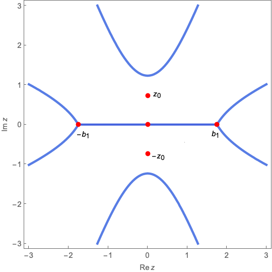
(a) $\sigma=-1$

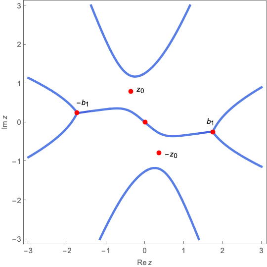
(b) $\sigma=-1+\textrm{i}$

(c) $\sigma=-1+1.6\textrm{i}$

(d) $\sigma_{\mbox{\tiny cr}}\simeq-1+1.7795\textrm{i}$

Figure 7. Snapshots of the continuous evolution of the critical graph $\mathscr{J}^{(1)}_{\sigma}$ as $\sigma$ changes from $-1$ in the vertical direction up to the critical value $\sigma_{\mbox{\tiny cr}}\simeq-1+1.7795\textrm{i}$ (locate the $\sigma$-values in Figure 1). At the critical value, just before the split of the support of the equilibrium measure, the point $z_{0}$ gets trapped between various portions of the critical graph.

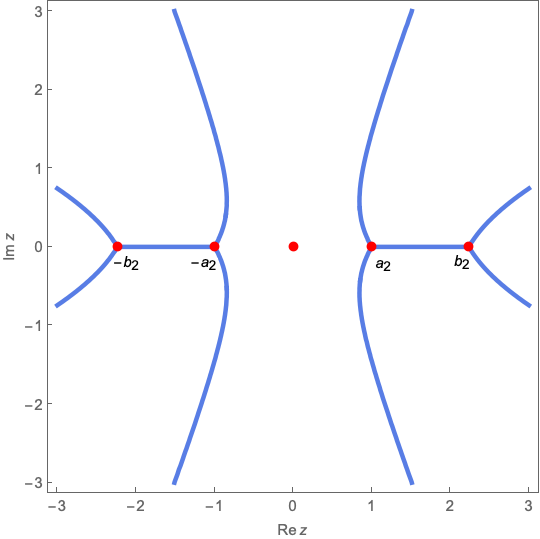
(a) $\sigma=-3$

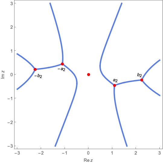
(b) $\sigma=-3+\textrm{i}$

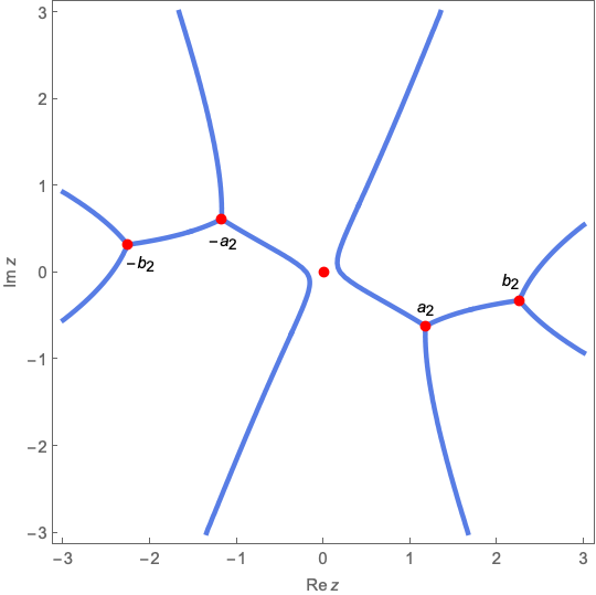
(c) $\sigma=-3+1.45\textrm{i}$

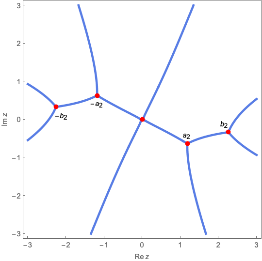
(d) $\sigma_{\mbox{\tiny cr}}\simeq-3+1.5025\textrm{i}$

Figure 8. Snapshots of the continuous evolution of the critical graph $\mathscr{J}^{(2)}_{\sigma}$ as $\sigma$ changes from $-3$ in the vertical direction up to the critical value $\sigma_{\mbox{\tiny cr}}\simeq-3+1.5025\textrm{i}$ (locate the $\sigma$-values in Figure 1). At the critical value, just before the birth of a cut at the origin, the origin gets trapped between different portions of the critical graph.

In Figures 9 through 11 we show how the support of the equilibrium measure evolves when it is altered from pre-critical one-cut or two-cut values to post-critical three-cut ones.

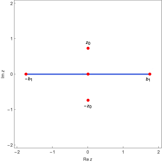
(a) $\sigma=-1$

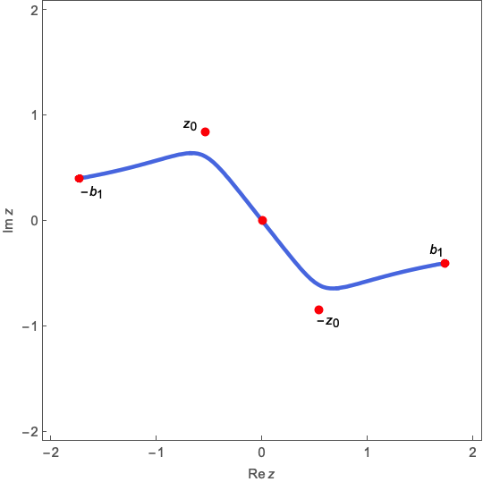
(b) $\sigma=-1+1.6\textrm{i}$

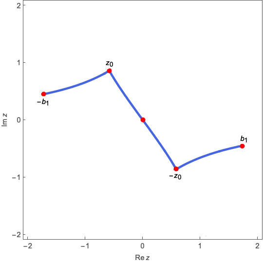
(c) $\sigma_{\mbox{\tiny cr}}\simeq-1+1.7795\textrm{i}$

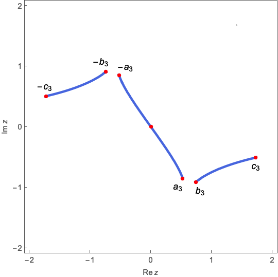
(d) $\sigma=-1+2\textrm{i}$

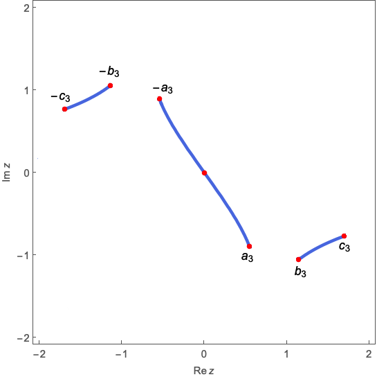
(e) $\sigma=-1+3\textrm{i}$

Figure 9. Snapshots of the continuous evolution of the support of the equilibrium measure in transition from the one-cut into the three-cut regime: the support of the equilibrium measure is at the onset of splitting into three symmetric cuts with respect to the origin at a critical value $\sigma_{\mbox{\tiny cr}}\in\gamma_{1}$ , See Figure 1.

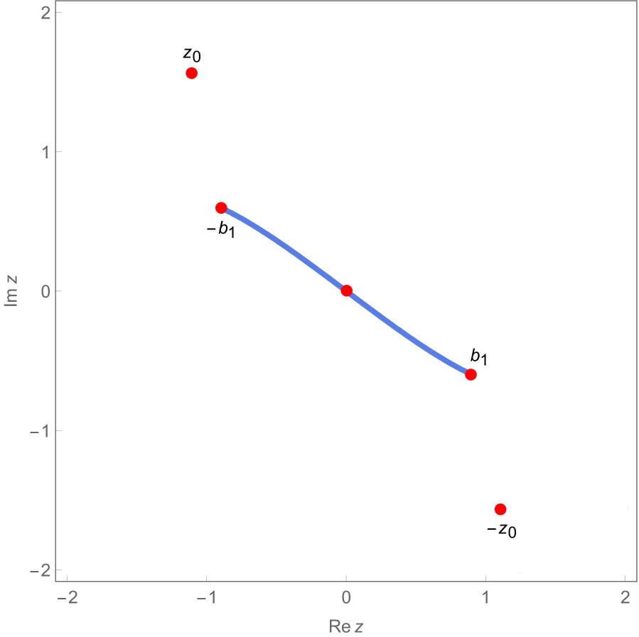
(a) $\sigma=1+4\textrm{i}$

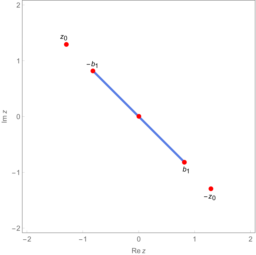
(b) $\sigma=4\textrm{i}$

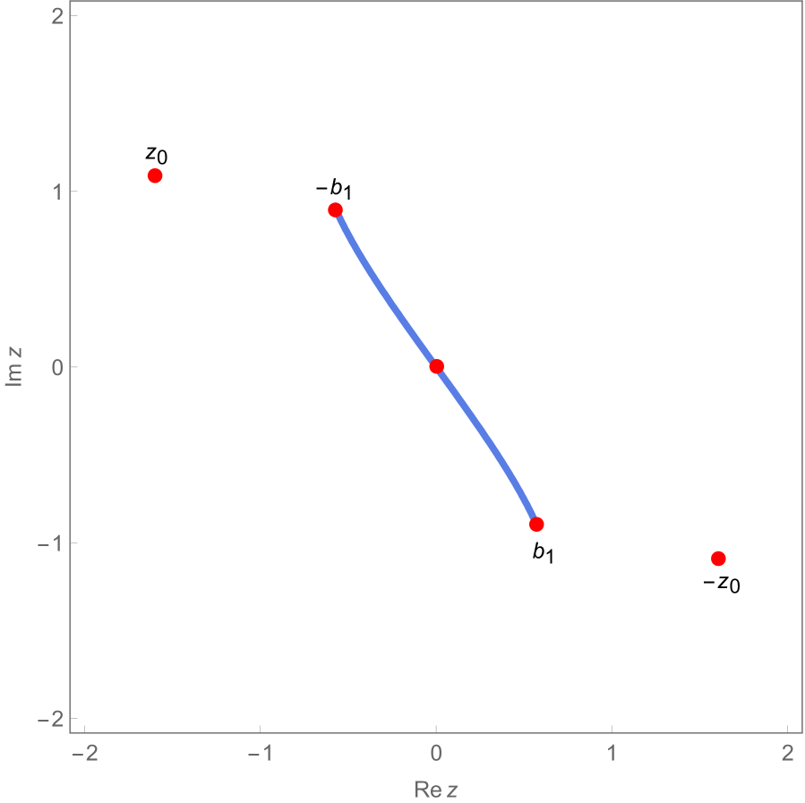
(c) $\sigma_{\mbox{\tiny cr}}\simeq-1.15+4\textrm{i}$

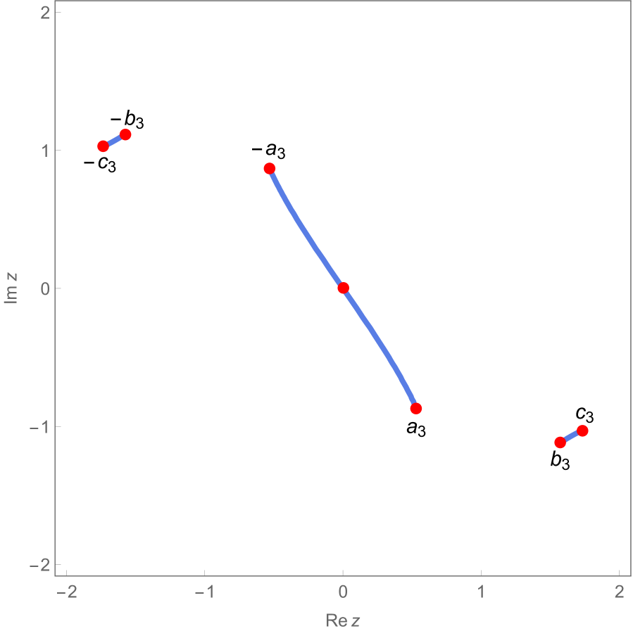
(d) $\sigma=-1.35+4\textrm{i}$

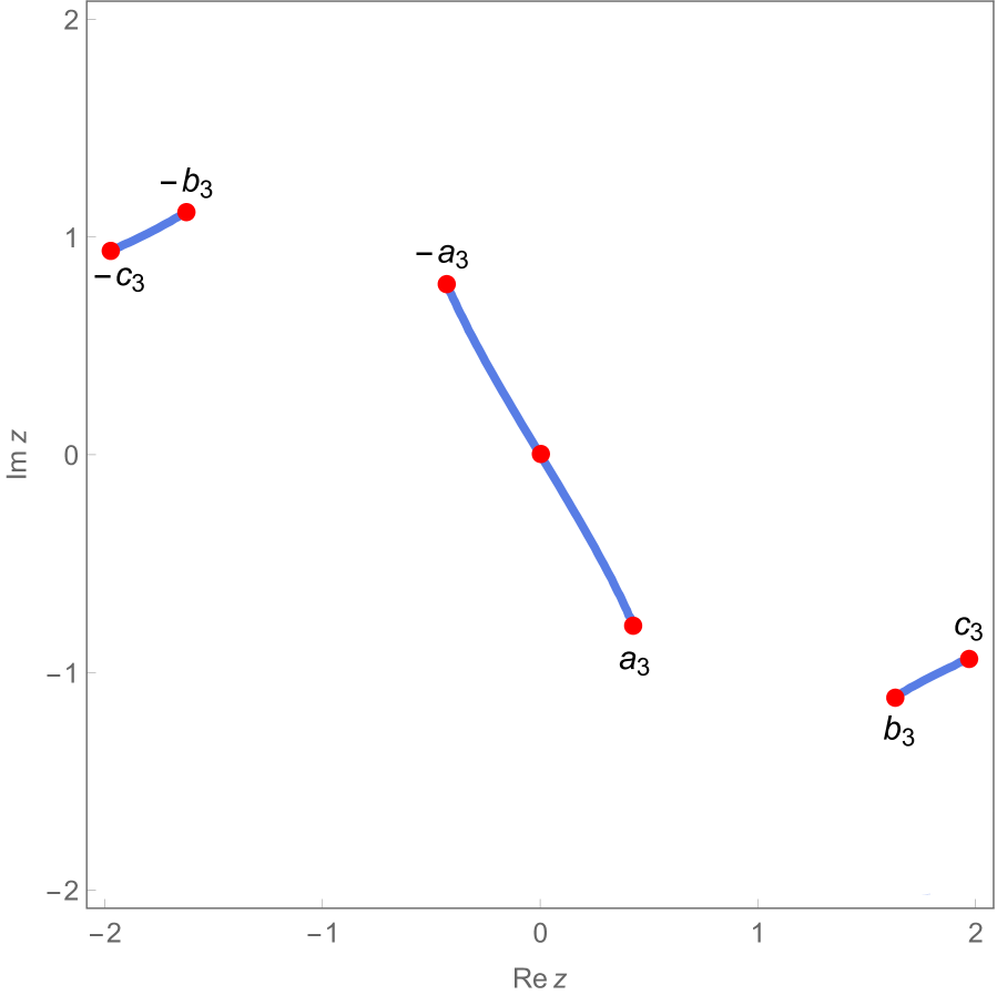
(e) $\sigma=-2+4\textrm{i}$

Figure 10. Snapshots of the continuous evolution of the support of the equilibrium measure in transition from the one-cut into the three-cut regime via birth of two symmetric cuts at $\pm z_{0}(\sigma_{\mbox{cr}})$, for some $\sigma_{\mbox{cr}}\in\gamma_{3}$, See Figure 1. Also, see Figure 14(b) to see the respective location of points with respect to the critical contours in the $\sigma$-plane.

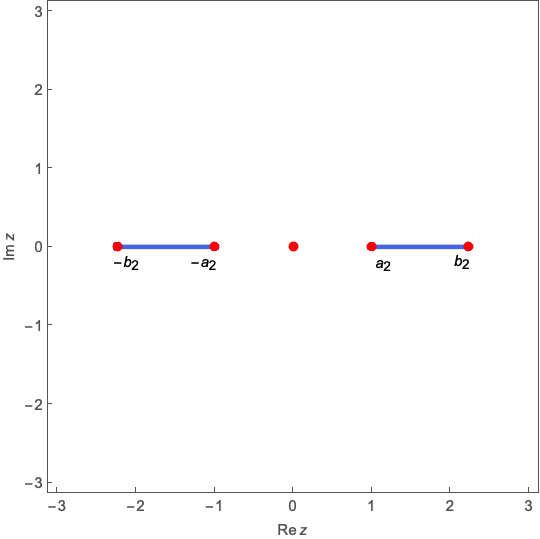
(a) $\sigma=-3$

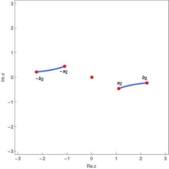
(b) $\sigma=-3+\textrm{i}$

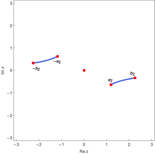
(c) $\sigma_{\mbox{\tiny cr}}=-3+1.5025\textrm{i}$

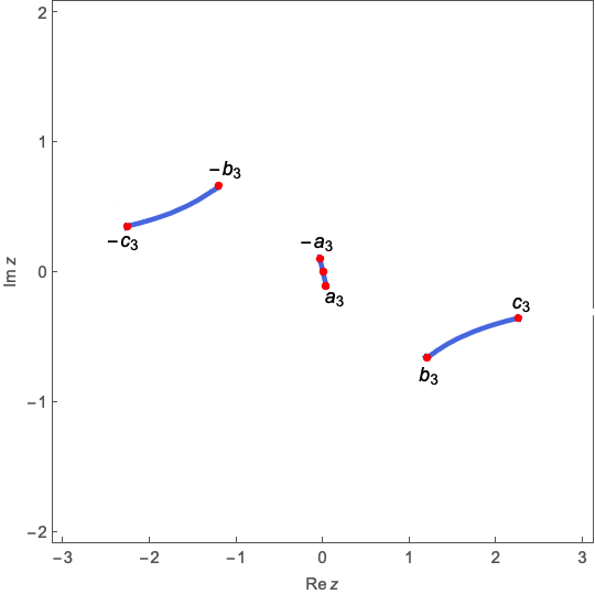
(d) $\sigma=-3+1.6\textrm{i}$

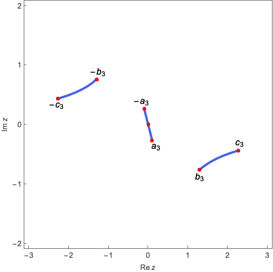
(e) $\sigma=-3+2\textrm{i}$

Figure 11. Snapshots of the continuous evolution of the support of the equilibrium measure in transition from the two-cut into the three-cut regime: at a critical value $\sigma_{\mbox{\tiny cr}}\in\gamma_{5}$ (see Figure 1) a cut is about to be born at the origin yielding a system of three symmetric cuts with respect to the origin.

4. Phase Diagram in the $\sigma$-plane and Auxiliary Quadratic Differentials

Similar to the approach taken in [BDY17], to analytically describe the transitions from the one-cut to the three-cut regime and from the two-cut to the three-cut regime we can use the critical trajectories of the associated auxiliary quadratic differentials.

4.1. One-cut to Three-cut Transition.

In this subsection we search for an analytic description for the values of $\sigma$ such that $z_{0}(\sigma)\in\mathscr{J}^{(1)}_{\sigma}$, that is $\Re[\Psi(\sigma)]=0$ where

(4.1) $$\begin{split}\Psi(\sigma)&:=\eta_{1}(z_{0}(\sigma);\sigma)=-\frac{\sigma}{4}\sqrt{\frac{1}{3}\left(-2\sigma-\sqrt{12+\sigma^{2}}\right)}\sqrt{-\sqrt{12+\sigma^{2}}}\\ &+2\log\left(\frac{\sqrt{\frac{1}{3}\left(-2\sigma-\sqrt{12+\sigma^{2}}\right)}+\sqrt{-\sqrt{12+\sigma^{2}}}}{\sqrt{\frac{2}{3}\left(-\sigma+\sqrt{12+\sigma^{2}}\right)}}\right).\end{split}$$

If we compute

(4.2) $$\left[\frac{\textrm{d}\Psi}{\textrm{d}\sigma}\right]^{2}=\frac{1}{12}\left(12+\sigma^{2}+2\sigma\sqrt{12+\sigma^{2}}\right),$$

we do not obtain a meromorphic quadratic differential, which is the preferred object to deal with (as opposed to what we had in (4.11)). However, if we express $\sigma$ and $z_{0}(\sigma)$ in terms of $b_{1}\equiv b_{1}(\sigma)$ via (2.35), then a direct calculation shows that in the variable $b_{1}$ we do obtain a meromorphic quadratic differential:

(4.3) $$\Xi(b_{1}):=\left[\frac{\textrm{d}\Psi}{\textrm{d}b_{1}}\right]^{2}=\frac{(16-b_{1}^{4})(16+3b_{1}^{4})^{3}}{256b_{1}^{10}}.$$

We can make things a bit simpler, as in the variable $\beta:=b_{1}^{2}$ we arrive at:

(4.4) $$\Xi(\beta)=\left[\frac{\textrm{d}\Psi}{\textrm{d}\beta}\right]^{2}=\frac{(16-\beta^{2})(16+3\beta^{2})^{3}}{1024\beta^{6}}.$$

Thus we can express $\Psi$ as

(4.5) $$\Psi(\beta)=\int^{\beta}_{-\frac{4\textrm{i}}{\sqrt{3}}}\sqrt{\Xi(s)}\textrm{d}s.$$

The initial point of integration is chosen to be $\beta=-4\textrm{i}/\sqrt{3}$ as this corresponds to $b_{1}=z_{0}$ (and $\sigma=i\sqrt{12}$) where $\Psi=0$. Therefore, the preimage (under the map $\sigma\mapsto\beta$) of the critical trajectories of the quadratic differential $\Xi(\beta)\textrm{d}\beta^{2}$ includes, and as described further below not equal to, the set $\{\sigma\ :\ \Re[\eta_{1}(z_{0}(\sigma);\sigma)]=0\}$. So one is naturally directed to study the critical trajectories of the auxiliary quadratic differential $\Xi(\beta)\textrm{d}\beta^{2}$. Notice that it has two simple zeros at $\pm 4$, two zeros of order three at $\pm 4\textrm{i}/\sqrt{3}$, a pole of order six at zero and a pole of order six at infinity (recall (3.9)). Therefore three critical trajectories emanate from $\beta=4$ and $\beta=-4$ each, while five critical trajectories emanate from $\beta=4\textrm{i}/\sqrt{3}$ and $\beta=-4\textrm{i}/\sqrt{3}$ each (Theorem $7.1$ of [Str84]). Also, there are 4 critical trajectories incident with $\beta=0$ and $\beta=\infty$ (Theorem $7.4$ of [Str84]). The local structure of the critical trajectories in a neighborhood of the critical points can be easily found by finding a ray on which $\Xi(\beta)\textrm{d}\beta^{2}<0$. Locally, the other critical trajectories will be then determined based on how many critical directions are incident with the critical point. For example it is simple to check that $\Xi(\beta)\textrm{d}\beta^{2}<0$ when $\beta=\varepsilon i+4\textrm{i}/\sqrt{3}$, $\varepsilon>0$. The other four critical directions at $4\textrm{i}/\sqrt{3}$ are now determined by forming equal angles $2\pi/5$ between adjacent critical directions. Similar analysis gives the local structure in the neighborhood of other critical points. At infinity $\Xi(\beta)\textrm{d}\beta^{2}\sim-\frac{27}{1024}\beta^{2}\textrm{d}\beta^{2}$, thus the integral of its square root behaves like $\frac{3\textrm{i}\sqrt{3}}{64}\beta^{2}$ and thus the four solutions to $\Re[\Psi(\beta)]=0$ near infinity respectively have asymptotic angles $0$, $\pi/2$, $\pi$, and $3\pi/2$. Using this for solutions near infinity, and having already determined the local critical structure near finite critical points, the only global structure (connection of critical trajectories) consistent with the Teichmüller’s lemma is shown in Figure 12. A calculation shows that $\Psi(\beta)$ as defined in (4.5) differs from $\Psi(-\beta)$ and from $\Psi(\overline{\beta})$ by additive purely imaginary quantities. This explains the symmetry with respect to the origin and the real axis in Figure 12.

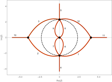
Figure 12. The red lines show the critical graph $\mathcal{T}$ of the auxiliary quadratic differential $2^{-10}\beta^{-6}(16-\beta^{2})(16+3\beta^{2})^{3}\textrm{d}\beta^{2}\equiv\Xi(\beta)\textrm{d}\beta^{2}$ in the $\beta$-plane. The black dots show the critical points of $\Xi(\beta)\textrm{d}\beta^{2}$: simple zeros at $\pm 4$, zeros of order three at $\pm 4\textrm{i}/\sqrt{3}$, pole of order six at zero. The actual critical graph in the $\sigma$-plane corresponding to the transition form the 1-cut regime to the 3-cut regime is a subset of the image of $\mathcal{T}$ under the Joukowsky map $\sigma=-\frac{3}{4}\beta+\frac{4}{\beta}$ (see Figure 13) which maps both the interior and the exterior of the circle of radius $4/\sqrt{3}$ onto the complement of the imaginary line segment in the $\sigma$-plane connecting $-\textrm{i}\sqrt{12}$ to $\textrm{i}\sqrt{12}$.

From (2.36) we can simply express $z^{2}_{0}$ and $\sigma$ in terms of $\beta$ as

(4.6) $$z^{2}_{0} =\frac{\beta}{4}+\frac{4}{\beta},$$

(4.7) $$\sigma =-\frac{3}{4}\beta+\frac{4}{\beta}.$$

We observe that the map from the $\beta$-plane to the $\sigma$-plane is a Joukowski map which maps both the interior and the exterior of the circle of radius $4/\sqrt{3}$ onto the complement of the imaginary line segment in the $\sigma$-plane connecting $-\textrm{i}\sqrt{12}$ to $\textrm{i}\sqrt{12}$. Therefore the image $\widehat{\Sigma}$ of the critical trajectories of $\Xi(\beta)\textrm{d}\beta^{2}$ in the $\beta$-plane under the Joukowsky map $\beta\mapsto\sigma$ provides all the candidates for the 1-cut to 3-cut phase transition in the $\sigma$-plane.

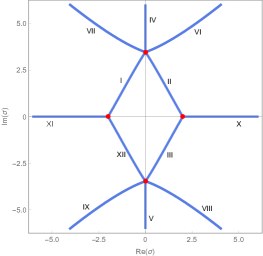
Figure 13. The image $\widehat{\Sigma}$ of the critical graph $\mathcal{T}$ of $2^{-10}\beta^{-6}(16-\beta^{2})(16+3\beta^{2})^{3}\textrm{d}\beta^{2}\equiv\Xi(\beta)\textrm{d}\beta^{2}$ under the Joukowsky map $\beta\mapsto\sigma=-\frac{3}{4}\beta+\frac{4}{\beta}$. The red dots at $\pm 2$ and $\pm\textrm{i}\sqrt{12}$ are the images of the critical points of $\Xi(\beta)\textrm{d}\beta^{2}$. The components I, II, III, IV, V, X, XI, and XII are the images of the parts of $\mathcal{T}$ in the exterior of the circle of radius $4/\sqrt{3}$, while the components VI, VII, VIII, and IX are the images of the parts of $\mathcal{T}$ in the interior of the circle of radius $4/\sqrt{3}$ (see Figure 12).

Inverting the Joukowsky map we obtain

(4.8) $$\beta^{(\pm)}(\sigma)=\frac{2}{3}\left(-\sigma\pm\sqrt{12+\sigma^{2}}\right).$$

We choose the branch cuts for the square root to be the two rays connecting $\textrm{i}\sqrt{12}$ to $-\infty+\textrm{i}\sqrt{12}$ and $-\textrm{i}\sqrt{12}$ to $-\infty-\textrm{i}\sqrt{12}$, and we fix the branch according to $\arg(\sigma-\textrm{i}\sqrt{12})=0$ for $\sigma=x+\textrm{i}\sqrt{12}$, and $\arg(\sigma+\textrm{i}\sqrt{12})=0$ for $\sigma=x-\textrm{i}\sqrt{12}$, $x>0$. However, recalling (2.37), our one-cut computations are based on $\beta^{(+)}$, not $\beta^{(-)}$. Therefore, among the twelve components of $\widehat{\Sigma}$, the actual candidates for 1-cut to 3-cut phase transition in the $\sigma$-plane are those which get mapped by $\beta^{(+)}$ to the critical trajectories of $\Xi(\beta)\textrm{d}\beta^{2}$ in the $\beta$-plane. By straight-forward calculations we observe that $\beta^{(+)}$ does not map the components of $\widehat{\Sigma}$ labeled by II, III, IV, V, and X to $\mathcal{T}$, while it does map the components of $\widehat{\Sigma}$ labeled by I, XII, VI, VII, VIII, IX, and XI respectively to the components of $\mathcal{T}$ labeled by $1$, $12$, $6$, $7$, $8$, $9$, and $11$ ( Actually it can be checked that $\beta^{(-)}$ maps the components of $\widehat{\Sigma}$ labeled by II, III, IV, V, and X respectively to the components of $\mathcal{T}$ labeled by $2$, $3$, $4$, $5$, and $10$ ). This means that the only places in the $\sigma$-plane at which 1-cut to 3-cut phase transition could happen are the components of $\widehat{\Sigma}$ labeled by I, XII, VI, VII, VIII, IX, and XI, see Figure 14(a).

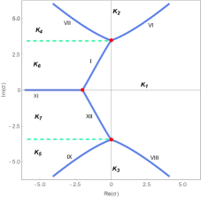
(a) The set $\widehat{\Sigma}$ shown in Figure 13 without its components labeled by II, III, IV, V, and X. Notice that $\beta^{(+)}$ maps the components of $\widehat{\Sigma}$ labeled by I, XII, VI, VII, VIII, IX, and XI respectively to the components of $\mathcal{T}$ labeled by $1$,$12$,$6$,$7$,$8$,$9$, and $11$, while it does not map the components of $\widehat{\Sigma}$ labeled by II, III, IV, V, and X to $\mathcal{T}$ (See Figures 12 and 13). We use the convention that the multicritical points at $\sigma=-2$ and $\sigma=\pm\textrm{i}\sqrt{12}$ belong to the critical lines incident to them, for instance $-2,\textrm{i}\sqrt{12}\in$ I. The green dashed lines represent the branch cuts $L_{\pm}$ (see Remark 2.1). To rigorously understand the boundaries of the one-cut region we study the sign of $\Re[\eta_{1}(\pm z_{0}(\sigma);\sigma)]$ in the infinite regions $\bm{K}_{i}$, $i=1,\cdots,5$.

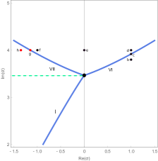
(b) An enlargement of Figure 14(a) around the point $\textrm{i}\sqrt{12}$ which shows the relative location of points B through H considered in Figure 3 with respect to the lines VI and VII. We recall that $b=1+3.8\textrm{i}$, $c\simeq 1+3.9187\textrm{i}$, $d=1+4\textrm{i}$, $e=4\textrm{i}$, $f=-1+4\textrm{i}$, $g\simeq-1.15+4\textrm{i}$, $h=-1.35+4\textrm{i}$. As shown in Figure 3, at the parameter values $c$ and $g$, the points $\pm z_{0}(\sigma)$ lie on the critical graph. At the parameter values $b$ and $h$, the points $\pm z_{0}(\sigma)$ belong to the unstable lands, while at the parameter values $d$, $e$, and $f$, the points $\pm z_{0}(\sigma)$ belong to stable lands. The alignment of the points $\pm b_{1}$ and $\pm z_{0}$ along the bisector of the second and fourth quadrants for $\sigma=\textrm{i}y$, with $y>\sqrt{12}$, is in particular shown for point $e$ in Figure 3(e).

Figure 14. Part (a) shows the remaining candidates (all values of $\sigma$ on the blue curves) for the one-cut to three-cut transitions. Part (b) shows an enlarged picture in a neighborhood of the tri-critical point $\textrm{i}\sqrt{12}$.

We will later show that for another reason the 1-cut to 3-cut phase transition could not happen along the component labeled by XI, and for yet another reason it can not happen along the components labeled by VI and VIII.

Lemma 4.1.

Let $\sigma\in$ I $\cup$ VI $\cup$ XII $\cup$ VIII  and different from $-2$ and $\pm\textrm{i}\sqrt{12}$. Then one of the following three possibilities holds:

• $\pm z_{0}(\sigma)\in J_{\sigma}$

• $z_{0}(\sigma)\in\ell_{2}^{(-b_{1}(\sigma))}$ and $-z_{0}(\sigma)\in\ell_{2}^{(b_{1}(\sigma))}$

• $z_{0}(\sigma)\in\ell_{3}^{(b_{1}(\sigma))}$ and $-z_{0}(\sigma)\in\ell_{3}^{(-b_{1}(\sigma))}$.

Proof.

This follows from continuous deformations of $z_{0}(\sigma)$ and $\mathscr{J}^{(1)}_{\sigma}$ with respect to $\sigma$. So we start from some $\sigma_{0}>-2$ where we know the structure $\mathscr{J}^{(1)}_{\sigma}$, and $\pm z_{0}(\sigma_{0})=\pm\textrm{i}y_{0}$, for some $y_{0}>0$ (See, e.g. Figure 7(a) for $\sigma_{0}=-1$). If we continuously deform $z_{0}(\sigma)$ and $\mathscr{J}^{(1)}_{\sigma}$ starting from $\sigma_{0}$ it is clear that $z_{0}(\sigma_{1})$ can only hit $J_{\sigma_{1}}$, $\ell_{2}^{(-b_{1}(\sigma_{1}))}$, or $\ell_{3}^{(b_{1}(\sigma_{1}))}$. The three possibilities in the statement of the Lemma now follow from Lemma 3.3, more precisely: i) if $z\in\ell_{2}^{(-b_{1}(\sigma))}$ then $-z\in\ell_{2}^{(b_{1}(\sigma))}$, ii) if $z\in\ell_{3}^{(-b_{1}(\sigma))}$ then $-z\in\ell_{3}^{(b_{1}(\sigma))}$, and iii) if $z\in J_{\sigma}$ then $-z\in J_{\sigma}$. ∎

Theorem 4.2.

For $\sigma\in\mbox{I}\cup\mbox{XII}$, it holds that $\pm z_{0}(\sigma)\in J_{\sigma}$.

Proof.

We only prove the theorem for $\sigma\in$ I, as the theorem for $\sigma\in$ XII can be proven identically. Notice that for $\sigma=-2\in$ I (see the caption of Figure 14(a)), we indeed have $\pm z_{0}(-2)=0\in J_{-2}=[-2,2]$. Obviously for all $\sigma\in$ I, we need to have $z_{0}(\sigma)$ either belong to $J_{\sigma}$ or to $\mathscr{J}_{\sigma}\setminus J_{\sigma}$. For the sake of arriving at a contradiction, let us assume that for some $\sigma_{1}\in$ I, $z_{0}(\sigma_{1})$ belongs to $\mathscr{J}_{\sigma}\setminus J_{\sigma}$. Due to continuity in deformations of $z_{0}(\sigma)$ and $\mathscr{J}_{\sigma}^{(1)}$, there has to be some intermediate $\sigma_{0}\in$ I between $\sigma=-2$ and $\sigma_{1}$ so that $z_{0}(\sigma_{0})$ simultaneously belongs to $J_{\sigma_{0}}$ and $\mathscr{J}_{\sigma_{0}}\setminus J_{\sigma_{0}}$. But this would lead to a geodesic polygon with two vertices at one of $\pm b_{1}(\sigma_{0})$ and $z_{0}(\sigma_{0})$ which is impossible due to Lemma 3.5. One gets the same contradiction using the identical argument for $-z_{0}(\sigma_{1})$. ∎

Lemma 4.3.

In $\bm{K}_{1}$ we have $\Re[\eta_{1}(\pm z_{0}(\sigma);\sigma)]>0$ while in $\bm{K}_{2}\cup\bm{K}_{3}$ we have $\Re[\eta_{1}(\pm z_{0}(\sigma);\sigma)]<0$.

Proof.

Consider the region $\bm{K}_{1}$ shown in Figure 14(a). under the map $\beta^{(+)}$ (see (4.8)) this region is mapped to the region bounded by the components 1, 12, 6, and 8 shown in Figure 12, which we denote by $K_{1}$. Also, the region $\bm{K}_{2}$ gets mapped by $\beta^{(+)}$ to the interior of the components 6 and 7 of Figure 12 , which we denote by $K_{2}$, while the region $\bm{K}_{3}$ is mapped by $\beta^{(+)}$ to the interior of the components 8 and 9 of Figure 12, which we denote by $K_{3}$.

Consider the conformal map (4.5) restricted to $K_{1}\cup K_{2}$. It is straightforward to see that $\Psi$ maps $K_{1}\cup K_{2}$ to the entire $\Psi$-plane, where $K_{1}$ is either mapped to the right-half or the left-half plane. Indeed, $\Psi$ maps $K_{1}$ to the right half plane and $K_{2}$ to the left half plane. To see this it is enough to find a single point $\beta_{0}\in K_{1}$ and show that $\Re[\Psi(\beta_{0})]>0$. Recall that the set $\{\sigma:\sigma>-2\}$ is inside $\bm{K}_{1}$, and its image $(0,4)\subset K_{1}$. From Lemma 3.16 we know that $\Re[\Psi(\beta)]>0$ for all $\beta\in(0,4)$ and thus for all $\beta\in K_{1}$, and consequently $\Re[\Psi(\beta)]<0$ for all $\beta\in K_{2}$. Consequently, $\Re\left[\Psi\left(\sigma\right)\right]>0$ for all $\sigma\in\bm{K}_{1}$ and $\Re\left[\Psi\left(\sigma\right)\right]<0$ for all $\sigma\in\bm{K}_{2}$.

Similarly, by considering the conformal map

$$\Psi_{*}(\beta)=\int^{\beta}_{\frac{4\textrm{i}}{\sqrt{3}}}\sqrt{\Xi(s)}\textrm{d}s,$$

restricted to $K_{1}\cup K_{3}$, we can show that $\Re\left[\Psi\left(\sigma\right)\right]<0$ for all $\sigma\in\bm{K}_{3}$. So we have justified that when $\sigma$ passes from $\bm{K}_{1}$ to $\bm{K}_{2}$ (resp. $\bm{K}_{3}$) through VI (resp. VIII), the function $\Re\left[\Psi\left(\sigma\right)\right]\equiv\Re\left[\eta_{1}\left(z_{0}(\sigma);\sigma\right)\right]$ changes sign from positive to negative, that is $z_{0}(\sigma)$ moves from an unstable land to a stable land. We have the same conclusion for $-z_{0}(\sigma)$ due to (3.7). ∎

Theorem 4.4.

It holds that

• $-z_{0}(\sigma)\in\ell_{2}^{(b_{1})}$ and $z_{0}(\sigma)\in\ell_{2}^{(-b_{1})}$ for $\sigma\in\mbox{VI}$,

• $z_{0}(\sigma)\in\ell_{3}^{(b_{1})}$ and $-z_{0}(\sigma)\in\ell_{3}^{(-b_{1})}$, for $\sigma\in\mbox{VIII}$,

• $-z_{0}(\sigma)\in\ell_{3}^{(b_{1})}$ and $z_{0}(\sigma)\in\ell_{3}^{(-b_{1})}$, for $\sigma\in\mbox{VII},$ and

• $z_{0}(\sigma)\in\ell_{2}^{(b_{1})}$ and $-z_{0}(\sigma)\in\ell_{2}^{(-b_{1})}$, for $\sigma\in\mbox{IX}$.

Proof.

We only prove this for $\sigma\in$ VI and $\sigma\in$ VII, as the proof for $\sigma\in$ VIII and $\sigma\in$ IX can be done identically. We first show this locally in an $\varepsilon$-neighborhood $D_{\varepsilon}(\textrm{i}\sqrt{12})$ of $\textrm{i}\sqrt{12}$, for small enough $\varepsilon>0$. Notice that as $\sigma$ approaches to $\textrm{i}\sqrt{12}$, $\mp z_{0}(\sigma)$ approaches to $\pm b_{1}(\sigma)$. So we consider the asymptotics of $\eta_{1}(-z_{0}(\sigma);\sigma)$ as $\sigma$ approaches to $\textrm{i}\sqrt{12}$. We indeed find that the order of vanishing is $5/4$:

(4.9) $$\eta_{1}(-z_{0}(\sigma);\sigma)=\frac{4\sqrt{2}}{5}3^{-1/8}e^{3\pi\textrm{i}/8}\left(\sigma-\textrm{i}\sqrt{12}\right)^{5/4}\left(1+O\left(\left(\sigma-\textrm{i}\sqrt{12}\right)^{1/4}\right)\right).$$

From the properties of the auxiliary quadratic differential we know that the local angle between the components labeled by $1$ and $6$ in Figure 12 is $2\pi/5$. The map (4.7) is not conformal at $\beta=-4\textrm{i}/\sqrt{3}$, indeed

$$\sigma(-\frac{4\textrm{i}}{\sqrt{3}})=\textrm{i}\sqrt{12},\qquad\sigma^{\prime}(-\frac{4\textrm{i}}{\sqrt{3}})=0,\qquad\sigma^{\prime\prime}(-\frac{4\textrm{i}}{\sqrt{3}})=-\frac{3\sqrt{3}}{8}\textrm{i}.$$

This means that the local angle at $\textrm{i}\sqrt{12}$ between the images I and VI (see Figure 14(a)) of $1$ and $6$ is $4\pi/5$. This analysis also gives us the local angles $\theta_{1},\theta_{6},\theta_{7}$ respectively of components I, VI, and VII made with the ray $x+\textrm{i}\sqrt{12}$, $x>0$:

$$\theta_{1}=\frac{-7\pi}{10},\qquad\theta_{6}=\frac{\pi}{10},\qquad\theta_{7}=\frac{9\pi}{10},\qquad\mbox{where}\qquad\sigma-\textrm{i}\sqrt{12}=\rho e^{\textrm{i}\theta},\qquad-\pi<\theta<\pi.$$

We can now notice that

• If $\sigma\in$ I, the leading order approximation of $\eta_{1}(-z_{0}(\sigma);\sigma)$ given by (4.9), is purely imaginary $\textrm{i}y_{1}(\rho)$, with $y_{1}(\rho)<0$,as $3\pi/8+5\theta_{1}/4=-\pi/2$,

• If $\sigma\in$ VI, the leading order approximation of $\eta_{1}(-z_{0}(\sigma);\sigma)$ given by (4.9), is purely imaginary $\textrm{i}y_{6}(\rho)$, with $y_{6}(\rho)>0$, as $3\pi/8+5\theta_{6}/4=\pi/2$, and

• If $\sigma\in$ VII, the leading order approximation of $\eta_{1}(-z_{0}(\sigma);\sigma)$ given by (4.9), is purely imaginary $\textrm{i}y_{7}(\rho)$, with $y_{7}(\rho)<0$, as $3\pi/8+5\theta_{7}/4=3\pi/2$.

This means that as $\sigma$ approaches to VI, from $\bm{K}_{1}\cap D_{\varepsilon}(\textrm{i}\sqrt{12})$, $-z_{0}(\sigma)$ must approach $\ell^{(b_{1}(\sigma))}_{2}$ from the right (We orient $\ell^{(b_{1}(\sigma))}_{2}$, $\ell^{(b_{1}(\sigma))}_{3}$, $\ell^{(-b_{1}(\sigma))}_{2}$, and $\ell^{(-b_{1}(\sigma))}_{3}$ in the outward direction as they emanate from $\pm b_{1}(\sigma)$), where we know that $\Im(\eta(z;\sigma))>0$ (See Figures 2(a) and 2(b)), and as $\sigma$ approaches to VII, from $\bm{K}_{2}\cap D_{\varepsilon}(\textrm{i}\sqrt{12})$, $-z_{0}(\sigma)$ must approach from the right to $\ell^{(b_{1}(\sigma))}_{3}$ where we know that $\Im(\eta(z;\sigma))<0$ by the identical conformal mapping arguments used to draw the Figures 2(a) and 2(b). Notice in the latter case, $-z_{0}(\sigma)$ can not approach the support $J_{\sigma}$ where we also know $\Im(\eta(z;\sigma))<0$. This is because it has to do so via the unstable lands, while in $\bm{K}_{2}$ we know that $\Re[\eta(-z_{0}(\sigma);\sigma)]<0$. The symmetry implies that as $\sigma$ approaches to VI, from $\bm{K}_{1}\cap D_{\varepsilon}(\textrm{i}\sqrt{12})$, $z_{0}(\sigma)$ must approach $\ell^{(-b_{1}(\sigma))}_{2}$ from the right, and as $\sigma$ approaches to VII, from $\bm{K}_{2}\cap D_{\varepsilon}(\textrm{i}\sqrt{12})$, $z_{0}(\sigma)$ must approach from the right to $\ell^{(-b_{1}(\sigma))}_{3}$.

Now we extend this local result to the entirety of VI and VII using the same argument presented in Theorem 4.2.

∎

Due to Lemma 4.4, the values of $\sigma\in\mbox{VI}\cup\mbox{VIII}$ do not belong to $\mathcal{O}^{*}_{1}$. However, in the following Theorem we show that they do belong to the larger set $\mathcal{O}_{1}$ (recall the Definitions 3.1 and 3.10).

Theorem 4.5.

All $\sigma\in\mbox{VI}\cup\mbox{VIII}$ belong to $\mathcal{O}_{1}$.

Proof.

By Theorem 4.4, at $\sigma_{*}\in$ VI, we have $-z_{0}(\sigma_{*})\in\ell_{2}^{(b_{1})}$ and $z_{0}(\sigma_{*})\in\ell_{2}^{(-b_{1})}$. By Lemma 3.15, there are no disconnected components for the critical graph and one has four critical trajectories incident at right angles at both $\pm z_{0}(\sigma_{*})$. Among these four critical trajectories, two must come from the two legs $\mathcal{L}^{(\sigma_{*})}_{2,l}$ and $\mathcal{L}^{(\sigma_{*})}_{2,r}$ of $\mathcal{L}^{(\sigma_{*})}_{2}$ which make a $\pi/2$ angle with each other at $-z_{0}(\sigma_{*})$ and approach to infinity respectively along the directions $-5\pi/8$ and $-3\pi/8$, while the other two must come from $\ell_{2}^{(b_{1})}$ folding at a $\pi/2$ angle into a short critical trajectory $\hat{\ell}^{(b_{1}(\sigma_{*}))}_{2}$ (connecting $b_{1}(\sigma_{*})$ to $-z_{0}(\sigma_{*})$) and another component $\check{\ell}^{(b_{1}(\sigma_{*}))}_{2}$ connecting $z_{0}(\sigma_{*})$ to infinity along the angle $-\pi/8$. Notice that $\ell_{3}^{(b_{1})}$ must still approach to infinity at the angle $\pi/8$ when $\sigma_{*}\in$ VI, due to continuity of deformations and that it has not been hit by $\pm z_{0}(\sigma_{*})$. Thus, when $\sigma_{*}\in$ VI, one still has the region $\Omega^{(\sigma_{*})}_{1}$ which encompasses $(M(\sigma_{*}),\infty)$ for some $M(\sigma_{*})>0$ (See Figure 3(c)).

Notice that there is still a single connection from $-b_{1}(\sigma_{*})$ to $b_{1}(\sigma_{*})$ to avoid having too many solutions at $\infty$. This proves that any $\sigma\in$ VI belongs to $\mathcal{O}_{1}$. An identical argument shows that any $\sigma\in$ VIII belongs to $\mathcal{O}_{1}$. ∎

Theorem 4.6.

The regions $\bm{K}_{2}$ and $\bm{K}_{3}$ shown in Figure 14(a) both belong to $\mathcal{O}^{*}_{1}$.

Proof.

We only prove this for $\bm{K}_{2}$ as the proof for $\bm{K}_{3}$ is identical. As $\sigma$ moves from $\sigma_{*}\in$ VI to some $\sigma_{1}\in\bm{K}_{2}$, $\pm z_{0}(\sigma_{1})$ must lie in $\sigma_{1}$-stable lands by Lemma 4.3. Recalling Figure 3(c) for $\sigma_{*}\in$ VI, this is only possible if at the onset of the entrance of $z_{0}$ into the stable lands, $\mathcal{L}^{(\sigma_{*})}_{2,l}$ and $\hat{\ell}^{(b_{1}(\sigma_{*}))}_{2}$ form the new $\ell^{(b_{1})}_{2}$ and $\mathcal{L}^{(\sigma_{*})}_{2,r}$ and $\check{\ell}^{(b_{1}(\sigma_{*}))}_{2}$ form the new hump $\mathcal{L}^{(4)}_{\sigma}$ (these notations are introduced partially in the proof of Theorem 4.5 and in the statement of Theorem 3.13), as the other possibility where $\hat{\ell}^{(b_{1}(\sigma_{*}))}_{2}$ and $\check{\ell}^{(b_{1}(\sigma_{*}))}_{2}$ form the new $\ell^{(b_{1})}_{2}$ is not allowed by the Teichmüller’s lemma regardless of which stable land $z_{0}$ enters. This means that one indeed has Figure 3(d) once $\sigma$ moves from $\sigma_{*}\in$ VI to some $\sigma_{1}\in\bm{K}_{2}$. Since at $\sigma_{1}$, $\ell^{(b_{1})}_{3}$ still approaches to $\infty$ along the $\pi/8$ direction, $\ell^{(b_{1})}_{2}$ approaches to $\infty$ along the $-5\pi/8$ direction. At $\sigma_{1}$ one indeed has a contour $\Gamma_{\sigma_{1}}(b_{1}(\sigma_{1}),\infty)$ entirely in the stable lands which encompasses $(M(\sigma_{1}),\infty)$ for some $M(\sigma_{1})>0$ (See the orange dashed lines in Figure 3(d)). One always has this connection to infinty as long as $z_{0}(\sigma)$ does not hit $\ell^{(b_{1})}_{3}$ which could block this access to the positive real axis (See Figures 3(e) and 3(f)). But for all $\sigma\in\bm{K}_{2}$ this does not happen which finishes the proof that $\bm{K}_{2}\subset\mathcal{O}^{*}_{1}$. ∎

Theorem 4.7.

The lines VII and IX form part of the boundaries of the one-cut region. More precisely, for all $\sigma\in$ VII $\cup$ IX, and all $\sigma\in\bm{K}_{4}\cup\bm{K}_{5}$ the one-cut definition does not hold.

Proof.

We only provide the proof for $\sigma\in$ VII $\cup\bm{K}_{4}$, as the proof for $\sigma\in$ IX $\cup\bm{K}_{5}$ is exactly identical. Recall that by $\bm{K}_{4}$, we denote the infinite region in the $\sigma$-plane bounded by $L_{+}$ and VII (see Remark 2.1 and Figure 14(a)). At $\sigma_{*}\in$ VII, by Theorem 4.4, we know that $\pm z_{0}(\sigma_{*})\in\ell^{(\mp b_{1}(\sigma_{*}))}_{3}$, and by a similar reasoning to that provided in the proof of Theorem 4.5, we know that the structure of the stable and unstable lands are as depicted in Figure 3(g). This shows that no $\sigma\in$ VII belongs to $\mathcal{O}_{1}$ since the third requirement of Definition 3.1 can not be met.

We denote the four critical trajectories incident with $-z_{0}(\sigma_{*})$, as

• $\mathcal{L}^{(\sigma_{*})}_{4,l}$ and $\mathcal{L}^{(\sigma_{*})}_{4,r}$ obtained from folding of $\mathcal{L}^{(\sigma_{0})}_{4}$ in two perpendicular components at $-z_{0}(\sigma_{*})$, in the limiting process $\bm{K}_{2}\ni\sigma_{0}\to\sigma_{*}\in$ VII (for the notation $\mathcal{L}_{4}$ recall Lemma 3.13),

• the short critical trajectory $\hat{\ell}^{(b_{1}(\sigma_{*}))}_{3}$ (connecting $b_{1}(\sigma_{*})$ to $-z_{0}(\sigma_{*})$), and $\check{\ell}^{(b_{1}(\sigma_{*}))}_{3}$ connecting $z_{0}(\sigma_{*})$ to infinity along the angle $\pi/8$, which are obtained from folding of $\ell^{(b_{1}(\sigma_{0}))}_{3}$ in two perpendicular components at $-z_{0}(\sigma_{*})$, in the limiting process $\bm{K}_{2}\ni\sigma_{0}\to\sigma_{*}\in$ VII.

By a similar argument to that shown in the proof of Lemma 4.3, we can show that $\Re[\eta_{1}(\pm z_{0}(\sigma);\sigma)]>0$ for all $\sigma\in\bm{K}_{4}$. In other words, as $\sigma$ moves from $\sigma_{*}\in$ VII to some $\sigma_{1}\in\bm{K}_{4}$, $\pm z_{0}(\sigma_{1})$ must lie in $\sigma_{1}$-unstable lands. This is only possible if at the onset of the entrance of $z_{0}$ into the unstable lands, $\mathcal{L}^{(\sigma_{*})}_{4,l}$ and $\hat{\ell}^{(b_{1}(\sigma_{*}))}_{3}$ together form the new $\ell^{(b_{1})}_{3}$ and $\mathcal{L}^{(\sigma_{*})}_{4,r}$ and $\check{\ell}^{(b_{1}(\sigma_{*}))}_{3}$ together form the new hump which provides the necessary solutions at $\infty$. Notice that the other possibilities lead to contradiction with Teichmüller’s lemma, regardless of which unstable land $z_{0}$ enters. This means that one indeed has the Figure 3(h), which proves that all $\sigma\in\bm{K}_{4}$ can not belong to $\mathcal{O}_{1}$ as the third requirement of Definition 3.1 can not be met.

∎

Theorem 4.8.

The lines I and XII form part of the boundaries of the one-cut region. More precisely, for all $\sigma\in$ I $\cup$ XII, and all $\sigma\in\bm{K}_{6}\cup\bm{K}_{7}$ the one-cut definition does not hold.

Proof.

We only provide the proof for $\sigma\in$ I $\cup\bm{K}_{6}$, as the proof for $\sigma\in$ XII $\cup\bm{K}_{7}$ is exactly identical. First notice that on I the second requirement of Definition 3.1 can not be met due to Theorem 4.2.

Now we show that any point $\sigma\in\bm{K}_{6}$ does not belong to $\mathcal{O}^{*}_{1}$. For the sake of arriving at a contradiction, assume that there exists a $\sigma_{1}\in\bm{K}_{6}$ which belongs to $\mathcal{O}^{*}_{1}$. We can now deform the branch-cut $L_{+}$ (see Remark 2.1) so that the point $\sigma_{1}$ and the component VII lie on the same side of $L_{+}$. But since $\mathcal{O}^{*}_{1}$ is open, this means that all $\sigma$ bounded by the deformed branch cut $L_{+}$, and the component VII must belong to $\mathcal{O}^{*}_{1}$. This contradicts Theorem 4.7. ∎

Theorems 4.5, 4.6, 4.7, 4.8 and the fact that $\bm{K}_{1}\subset\mathcal{O}^{*}_{1}$ can be formulated as the following Theorem.

Theorem 4.9.

The one-cut region is the region labeled so in Figure 1.

This characterization, immediately implies the openness on the one-cut region.

Corollary 4.9.1.

The set $\mathcal{O}_{1}$ is open.

4.2. Two-cut to Three-cut Transition.

Due to the symmetry with respect to the origin, the transition from the two-cut regime to the three-cut regime could only occur through birth of a cut at the origin. Define

(4.10) $$\Phi(\sigma):=\eta_{2}(0;\sigma)=-\frac{\sigma\sqrt{\sigma^{2}-4}}{4}+\log\left[\frac{\sigma+\sqrt{\sigma^{2}-4}}{2}\right].$$

The values of $\sigma$ for which such a transition takes place are those at which the real part of (4.10) vanishes. A calculation shows

(4.11) $$\Upsilon(\sigma):=\left[\frac{\textrm{d}\Phi}{\textrm{d}\sigma}\right]^{2}=\frac{1}{4}(\sigma^{2}-4).$$

Thus the auxiliary quadratic differential associated to the transition from the two-cut regime to the three-cut regime is $\Upsilon(\sigma)\textrm{d}\sigma^{2}$, since we can express $\Phi(\sigma)$ as

(4.12) $$\Phi(\sigma)=\int_{2}^{\sigma}\sqrt{\Upsilon(s)}\textrm{d}s,$$

where we have chosen the lower bound of integration as such since at $\Phi(2)=0$. The auxiliary quadratic differential $\Upsilon(\sigma)\textrm{d}\sigma^{2}$ has two simple zeros at $\pm 2$ and a pole of order $6$ at infinity (recall (3.9)). Therefore three critical trajectories emanate from $\sigma=2$ and $\sigma=-2$ each, and four critical trajectories are incident with infinity. At infinity $\Upsilon(\sigma)\textrm{d}\sigma^{2}\sim\frac{1}{4}\sigma^{2}\textrm{d}\sigma^{2}$, thus the integral of its square root behaves like $\frac{1}{4}\sigma^{2}$ and thus the four solutions to $\Re[\Phi(\sigma)]=0$ near infinity respectively have asymptotic angles $\pi/4$, $3\pi/4$, $5\pi/4$, and $7\pi/4$. Since $\Upsilon(\sigma)\textrm{d}\sigma^{2}<0$ at any point in $(-2,2)$, we can immediately determine the local structure of critical trajectories at $\pm 2$. A calculation shows that $\Phi(\sigma)$ as defined in (4.12) differs from $\Phi(-\sigma)$ and from $\Phi(\bar{\sigma})$ by additive purely imaginary quantities which imposes a symmetry with respect to the origin and with respect to the real axis in the critical graph of $\Upsilon(\sigma)\textrm{d}\sigma^{2}$, which also means that one has a symmetry with respect to the imaginary axis as well. This symmetry ensures that the geodesic polygon with vertices $\sigma=2$ and $\infty$ must entirely lie in the right half-plane, because if the polygon were to hit the imaginary axis at say $\textrm{i}y_{*}$, it would make $\sigma=\textrm{i}y_{*}$ (and also $\sigma=-\textrm{i}y_{*}$) a non-regular point of the quadratic differential $\Upsilon(\sigma)\textrm{d}\sigma^{2}$, which is a contradiction (recall that through each regular point of a meromorphic quadratic differential passes exactly one $\theta$-arc). Based on what we discussed above and what we know about the asymptotic angles at infinity, the critical graph shown in Figure 15 is indeed correct.

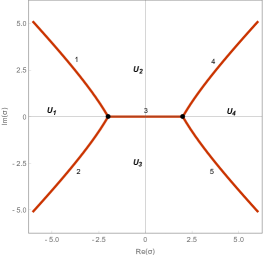
Figure 15. The critical graph $\textstyle\widehat{\vrule width=0.0pt,height=6.14998pt\vrule height=0.0pt,width=6.50002pt}$ $\textstyle\Sigma$ of the auxiliary quadratic differential $\frac{1}{4}(\sigma^{2}-4)\textrm{d}\sigma^{2}\equiv\Upsilon(\sigma)\textrm{d}\sigma^{2}$ whose components are the candidates for the two-cut to the three-cut transition. The black dots show the critical points of $\Upsilon(\sigma)\textrm{d}\sigma^{2}$ which are simple zeros at $\pm 2$.

We can prove the following Lemma similarly as we proved Lemma 4.3, thus we do not provide the details.

Lemma 4.10.

In $\bm{U}_{1}$ we have $\Re[\eta_{2}(0;\sigma)]<0$ while in $\bm{U}_{2}\cup\bm{U}_{3}$ we have $\Re[\eta_{2}(0;\sigma)]>0$.

Theorem 4.11.

The two-cut regime is the region labeled so in Figure 1.

Proof.

Firstly, recalling Lemma 3.26 and Theorem 3.22 we can show that $\bm{U}_{1}\subset\mathcal{O}_{2}$. By Corollary 3.25.1, none of the lines labeled by $\bm{1}$ to $\bm{5}$ in Figure 15 belong to $\mathcal{O}_{2}$. Now, we show that no $\sigma\in\bm{U}_{4}$ can belong to $\mathcal{O}_{2}$. Indeed as described above, the region $\bm{U}_{4}$ must lie entirely in the right half plane which itself belongs to the one-cut region by Theorem 4.9, so $\bm{U}_{4}\subset\mathcal{O}_{1}$. Due to the uniqueness of the support of the equilibrium measure no $\sigma\in\bm{U}_{4}$ can belong to $\mathcal{O}_{2}$. Recalling Lemma 3.25, we know that for $\sigma_{0}\in\bm{1}$, either $\ell^{(a_{2})}_{2}$ must connect to $\ell^{(-a_{2})}_{2}$, or $\ell^{(a_{2})}_{3}$ must connect to $\ell^{(-a_{2})}_{3}$ at the origin (see, e.g. Figure 5(b)). Similar to the argument provided in Theorem 4.7 we can show that the only possible transition for the critical graph of $Q_{2}(z;\sigma)\textrm{d}z^{2}$ as $\bm{1}\ni\sigma_{0}\to\sigma_{1}\in\bm{U}_{2}$ is the one shown from Figure 5(b) to Figure 5(c). This makes sure that no point in $\bm{U}_{2}$ could belong to $\mathcal{O}_{2}$ (recall Theorem 3.22). Identically one can show that no point in $\bm{U}_{3}$ could belong to $\mathcal{O}_{2}$. ∎

Remark 4.12.

The line labeled by VII (resp. IX) in Figure 14(a) has no intersection with the line labeled by $\bm{1}$ (resp. $\bm{2}$) in Figure 15. This is obvious due to the uniqueness of the support of the equilibrium measure. Indeed, if there was an intersection point $\sigma$, then it would simultaneously be a degenerate one-cut and a degenerate two-cut $\sigma$. Another contradiction would be that if there was an intersection point $\sigma$, then we would have had a way to continuously make a transition from a two-cut $\sigma_{2}$ to a one-cut $\sigma_{1}$ through some $\bm{1}\ni\sigma_{0}\neq-2$. But we know that the only way for such a transition is through degeneration of the gap from $-a_{2}$ to $a_{2}$, that is $\pm a_{2}\to 0$ which is only possible if $\sigma\to-2$ (recall (2.60)).

Theorem 4.13.

The three-cut regime is the region labeled so in Figure 1.

Proof.

By Theorems 4.9 and 4.11 we have already proven that in the region labeled as the "three-cut regime" in Figure 1 the one-cut and two-cut requirements are not satisfied. Since for all $\sigma$, the equilibrium measure and the Riemann-Hilbert contour exists and is unique (see [KS15], where uniqueness of the contour outside of the support of the equilibrium measure is up to homotopy) we conclude that all sigma in that region must necessarily satisfy the requirements of Definition 3.31. ∎

5. The Riemann-Hilbert Problem in the One-cut Regime, String Equations and Topological Expansion of the Recurrence Coefficients

In this section we follow [BI05]. For simplicity of notation, let us use $b$ instead of $b_{1}$ in this section. Assume that $\sigma$ belongs to the one-cut regime and let us consider the set of monic orthogonal polynomials $P_{n}(z;N)$, $\deg P_{n}(z;N)=n$, satisfying

(5.1) $$\int_{\Gamma_{\sigma}}P_{n}(s;N)P_{k}(s;N)e^{-NV(s)}\textrm{d}s=h_{n}(N)\delta_{n,k},\qquad k=0,1,\cdots,n,$$

where we suppress the dependence on $\sigma$ in all of the quantities and functions. Since the potential $V$ is even, these polynomials satisfy the following recurrence relation

(5.2) $$zP_{n}(z;N)=P_{n+1}(z;N)+\gamma^{2}_{n}(N)P_{n-1}(z;N).$$

Corresponding to this system of orthogonal polynomials one has the following Riemann-Hilbert problem [FIK92]

• RH-$\bm{Y}$1 $\qquad Y(z;n,N)$ is holomorphic in ${\mathbb{C}}\setminus\Gamma_{\sigma}$.

• RH-$\bm{Y}$2 $\qquad Y_{+}(z;n,N)=Y_{-}(z;n,N)J_{Y}(z;N),\quad z\in\Gamma_{\sigma},\qquad$ where

  (5.3) $$J_{Y}(z;N)=\begin{pmatrix}1&w(z;N)\\ 0&1\end{pmatrix},\qquad\qquad w(z;N):=e^{-NV(z)}.$$

• RH-$\bm{Y}$3 $\qquad Y(z;n,N)=(I+O(z^{-1}))\begin{pmatrix}z^{n}&0\\ 0&z^{-n}\end{pmatrix},\quad\text{as}\quad z\to\infty$.

The representation of the solution of this Riemann-Hilbert problem in terms of OPs is due to Fokas, Its and Kitaev [FIK92] and is given by

(5.4) $$\begin{pmatrix}P_{n}(z;N)&\mathscr{C}[P_{n}w](z;N)\\ -\displaystyle\frac{2\pi\textrm{i}}{h_{n-1}(N)}P_{n-1}(z;N)&-\displaystyle\frac{2\pi\textrm{i}}{h_{n-1}(N)}\mathscr{C}[P_{n-1}w](z;N)\end{pmatrix},$$

where $\mathscr{C}[f]$ is the Cauchy transform of the function $f$ with respect to the contour $\Gamma_{\sigma}$. Using the three-term recurrence relation and the orthogonality conditions one can easily observe that

(5.5) $$\gamma_{n}^{2}(N)=\frac{h_{n}(N)}{h_{n-1}(N)}.$$

For a parameter $\varkappa>0$, define

(5.6) $$V_{\varkappa}(z;\sigma)\equiv V_{\varkappa}:=V/\varkappa.$$

Doing the one-cut endpoint calculations for $V_{\varkappa}$, similar to those done in §2.4.1, we find

(5.7) $$\rho_{V}(z;\sigma,\varkappa)=\frac{1}{2\pi\textrm{i}\varkappa}(z^{2}-z^{2}_{0}(\varkappa;\sigma))\left(\sqrt{z^{2}-b^{2}(\varkappa;\sigma)}\right)_{+},$$

and

(5.8) $$b(\varkappa;\sigma)=\sqrt{\frac{2}{3}\left(-\sigma+\sqrt{12\varkappa+\sigma^{2}}\right)}\quad\text{and}\quad z_{0}(\varkappa;\sigma)=\sqrt{\frac{1}{3}\left(-2\sigma-\sqrt{12\varkappa+\sigma^{2}}\right)}.$$

The multi-critical points are obtained when $z_{0}=b$ and when $z_{0}=0$, these possibilities respectively correspond to

(5.9) $$12\varkappa+\sigma^{2}=0,\quad\text{and}\quad-2\sigma-\sqrt{12\varkappa+\sigma^{2}}=0.$$

Therefore, the multi-critical points are

(5.10) $$\sigma=\pm\textrm{i}\sqrt{12\varkappa},\quad\text{and}\quad\sigma=-2\sqrt{\varkappa},$$

and we have a similar picture as Figure 1 for the critical lines corresponding to transition from the one-cut to the three-cut regime for $V_{\varkappa}$. We also have the following formulae for the corresponding $g$-function

(5.11) $$g(z;\sigma,\varkappa)=\frac{1}{\varkappa}g(z;\sigma,1),$$

and the Euler-Lagrange constant

(5.12) $$\ell^{(1)}_{*}(\sigma,\varkappa)=\frac{1}{\varkappa}\ell^{(1)}_{*}(\sigma,1),$$

where $g(z;\sigma,1)$, and $\ell^{(1)}_{*}(\sigma,1)$ are respectively given by (2.43) and (2.44).

Note that for $\sigma$ in the one-cut regime the expressions in (5.8) are locally analytic in $\sigma$ and $\varkappa$. In particular, for any fixed $\sigma$, there exists $\varepsilon(\sigma)>0$ such that $b(\varkappa;\sigma)$ and $z_{0}(\varkappa;\sigma)$ are analytic in $\varkappa$ in the interval

(5.13) $$1-\varepsilon(\sigma)<\varkappa<1+\varepsilon(\sigma),\qquad 0<\varepsilon(\sigma)<1.$$

In particular, let

(5.14) $$\varkappa=\frac{n}{N}.$$

For this choice of $\varkappa$, we have

(5.15) $$NV(z)=nV_{\varkappa}(z).$$

Note that the orthogonal polynomials (and hence their norms) with respect to $e^{-NV(z)}$ and $e^{-nV_{\varkappa}(z)}$ are identical as they are built by bordered Hankel determinants out of moments of the identical weight functions. The Riemann-Hilbert problem corresponding to $e^{-nV_{\varkappa}(z)}$ would be exactly similar to RH-$\bm{Y}$1 through RH-$\bm{Y}$3, except that one should make replacements $V\mapsto V_{\varkappa}$ and $N\mapsto n$ in RH-$\bm{Y}$2. As a result of the Riemann-Hilbert analysis for orthogonal polynomials on the line with respect to the weight $e^{-nV_{\varkappa}(z)}$ we obtain a $1/N$ asymptotic expansion for $\gamma^{2}_{n}$:

(5.16) $$R_{n}(\varkappa;\sigma):=\gamma^{2}_{n}(\varkappa;\sigma)\sim\sum^{\infty}_{j=0}\frac{r_{j}(\varkappa;\sigma)}{N^{j}},\quad\text{as}\quad N\to\infty,$$

where

(5.17) $$r_{0}(\varkappa;\sigma)\equiv\frac{b^{2}(\varkappa;\sigma)}{4}.$$

The Riemann-Hilbert analysis is standard and we do not provide the details here. For one-cut real potentials see e.g. [Cha18, CG21], and for complex one-cut potentials see e.g. [BDY17, BT15, KM01, KM04].

Now, recall (see e.g. [BL14]) the string equations

(5.18) $$\gamma_{n}[V^{\prime}(\mathcal{Q})]_{n,n-1}=\frac{n}{N},\quad\text{and}\quad[V^{\prime}(\mathcal{Q})]_{n,n}=0,$$

where

(5.19) $$\mathcal{Q}=\begin{pmatrix}0&\gamma_{1}&0&0&\cdots\\ \gamma_{1}&0&\gamma_{2}&0&\cdots\\ 0&\gamma_{2}&0&\gamma_{3}&\cdots\\ \vdots&\ddots&\ddots&\ddots&\cdots\\ \end{pmatrix}.$$

The relevant quantities reduce to:

(5.20) $$[\mathcal{Q}]_{n,n-1}=\gamma_{n},\qquad[\mathcal{Q}]_{n,n}=0,\qquad[\mathcal{Q}^{3}]_{n,n-1}=\gamma_{n}\gamma^{2}_{n-1}+\gamma_{n}^{3}+\gamma_{n}\gamma^{2}_{n+1},\qquad[\mathcal{Q}^{3}]_{n,n}=0.$$

Therefore the second string equation is automatically satisfied and the first one can be written as

(5.21) $$\gamma_{n}^{2}(\varkappa;\sigma)\left(\sigma+\gamma_{n}^{2}(\varkappa;\sigma)+\gamma_{n-1}^{2}(\varkappa;\sigma)+\gamma_{n+1}^{2}(\varkappa;\sigma)\right)=\varkappa,$$

or

(5.22) $$R_{n}(\varkappa;\sigma)\left(\sigma+R_{n-1}(\varkappa;\sigma)+R_{n}(\varkappa;\sigma)+R_{n+1}(\varkappa;\sigma)\right)=\varkappa.$$

Note that

(5.23) $$R_{n\pm 1}(\varkappa;\sigma)\sim\sum^{\infty}_{j=0}\frac{r_{j}(\varkappa\pm N^{-1},\sigma)}{N^{j}},\quad\text{as}\quad N\to\infty.$$

Evaluation of Taylor expansions of $r_{j}$, centered at $\varkappa=n/N$, at $\varkappa\pm N^{-1}$ yields

(5.24) $$R_{n+1}(\varkappa;\sigma)\sim\sum^{\infty}_{j=0}\frac{1}{N^{j}}\sum^{\infty}_{\ell=0}\frac{r^{(\ell)}_{j}(\varkappa;\sigma)}{\ell!N^{\ell}},\quad\text{as}\quad N\to\infty.$$

and

(5.25) $$R_{n-1}(\varkappa;\sigma)\sim\sum^{\infty}_{j=0}\frac{1}{N^{j}}\sum^{\infty}_{\ell=0}\frac{(-1)^{\ell}r^{(\ell)}_{j}(\varkappa;\sigma)}{\ell!N^{\ell}},\quad\text{as}\quad N\to\infty.$$

Direct computation gives the following asymptotic expansion for the left hand side of (5.21) in inverse powers of $N$:

(5.26) $$R_{n}(\varkappa;\sigma)\left(\sigma+R_{n-1}(\varkappa;\sigma)+R_{n}(\varkappa;\sigma)+R_{n+1}(\varkappa;\sigma)\right)\sim\sum^{\infty}_{j=0}\frac{\hat{r}_{j}(\varkappa;\sigma)}{N^{j}},$$

where

(5.27) $$\hat{r}_{j}(\varkappa;\sigma)=\sigma r_{j}(\varkappa;\sigma)+\sum^{j}_{\ell=0}r_{\ell}(\varkappa;\sigma)\left[3r_{j-\ell}(\varkappa;\sigma)+\sum^{j-\ell-1}_{m=0}(1+(-1)^{j-\ell-m})\frac{r^{(j-\ell-m)}_{m}(\varkappa;\sigma)}{(j-\ell-m)!}\right]$$

So the string equation (5.21) can be written as

(5.28) $$\hat{r}_{0}(\varkappa;\sigma)=\varkappa,\quad\text{and}\quad\hat{r}_{j}(\varkappa;\sigma)=0,\qquad j\in{\mathbb{N}}.$$

Lemma 5.1.

$\gamma^{2}_{n}(\sigma)$ has a power series expansion in in inverse powers of $N^{2}$.

Proof.

We prove that $r_{2k-1}(\varkappa;\sigma)=0$, $k\in{\mathbb{N}}$, by induction. For $k=1$ it can be seen as follows. Using (5.27) we write (5.28) for $j=1$ to get

(5.29) $$\hat{r}_{1}(\varkappa;\sigma)=r_{1}(\varkappa;\sigma)(\sigma+6r_{0}(\varkappa;\sigma))=0.$$

Using (5.8) and (5.17) we can show

(5.30) $$\sigma+6r_{0}(\varkappa;\sigma)=\sqrt{12\varkappa+\sigma^{2}},$$

which is nonzero as we are away from the multicritical points $\pm\textrm{i}\sqrt{12\varkappa}$ (see (5.9), (5.10) and above). Therefore

(5.31) $$r_{1}(\varkappa;\sigma)=0.$$

Assume that all $r_{2k-1}(\varkappa;\sigma)=0$, for $k\in 2,3,\cdots,k_{0}$ (induction hypothesis). So we can update the definition (5.16) of $\gamma_{n}$ to be

(5.32) $$R_{n}(\varkappa;\sigma)\sim\sum^{k_{0}-1}_{j=0}\frac{r_{2j}(\varkappa;\sigma)}{N^{2j}}+\sum^{\infty}_{j=2k_{0}}\frac{r_{j}(\varkappa;\sigma)}{N^{j}},\quad\text{as}\quad N\to\infty,$$

and thus we have analogues of equations (5.23), (5.24), (5.25), (5.26) and (5.27). Now we show that $r_{2k_{0}+1}(\varkappa;\sigma)=0$. Using (5.27) we write (5.28) for $j=2k_{0}+1$. Note that the functions $r_{2k-1}$, $1\leq k\leq k_{0}$ and their derivatives should be disregarded as being zero, due to the update in the definition of $\gamma_{n}$ by the induction hypothesis. Therefore we get

(5.33) $$\hat{r}_{2k_{0}+1}(\varkappa;\sigma)=r_{2k_{0}+1}(\varkappa;\sigma)(\sigma+6r_{0}(\varkappa;\sigma))=0,$$

which implies that $r_{2k_{0}+1}(\varkappa;\sigma)=0$, and thus

(5.34) $$R_{n}(\varkappa;\sigma)\sim\sum^{\infty}_{j=0}\frac{r_{2j}(\varkappa;\sigma)}{N^{2j}}.$$

∎

Here it is worthwhile to provide explicit formulae for some $r_{2k}$. We recall that $r_{0}$ is given by (5.17). Using (5.21), (5.27) and (5.28) we can show

(5.35) $$r_{2}(\varkappa;\sigma)=-\frac{r_{0}(\varkappa;\sigma)r^{{}^{\prime\prime}}_{0}(\varkappa;\sigma)}{\sigma+6r_{0}(\varkappa;\sigma)},$$

and

(5.36) $$r_{4}(\varkappa;\sigma)=-\frac{\frac{1}{12}r_{0}(\varkappa;\sigma)r^{(4)}_{0}(\varkappa;\sigma)+3r^{2}_{2}(\varkappa;\sigma)+r_{2}(\varkappa;\sigma)r^{{}^{\prime\prime}}_{0}(\varkappa;\sigma)+r_{0}(\varkappa;\sigma)r^{{}^{\prime\prime}}_{2}(\varkappa;\sigma)}{\sigma+6r_{0}(\varkappa;\sigma)}.$$

We can actually find the following recursive formula for all $r_{2j}$. Indeed,

(5.37) $$r_{2j}(\varkappa;\sigma)=-\frac{\Lambda_{2j}(\varkappa;\sigma)}{\sigma+6r_{0}(\varkappa;\sigma)},\qquad j\in{\mathbb{N}},$$

where

(5.38) $$\Lambda_{2j}(\varkappa;\sigma):=3\sum^{j-1}_{\ell=1}r_{2\ell}(\varkappa;\sigma)r_{2j-2\ell}(\varkappa;\sigma)+2\sum^{j-1}_{\ell=0}r_{2\ell}(\varkappa;\sigma)\sum^{j-\ell-1}_{m=0}\frac{r^{(2j-2\ell-2m)}_{2m}(\varkappa;\sigma)}{(2j-2\ell-2m)!}.$$

6. Topological Expansion of the Free Energy

Proposition 6.1.

For $\sigma$ in the one-cut regime we have

(6.1) $$\frac{\partial^{2}F}{\partial\sigma^{2}}=\frac{N^{2}}{4n^{2}}R_{n}(R_{n-1}+R_{n+1}),$$

and

(6.2) $$\frac{\partial F}{\partial\sigma}=-\frac{N^{2}}{2n^{2}}R_{n}(\frac{n}{N}+R_{n-1}R_{n+1}).$$

Proof.

By the Heine’s identity for Hankel determinants and noting that $h_{k}=D_{k+1}/D_{k}$, where $D_{k}$ is the $k\times k$ Hankel determinant generated by the weight $e^{-NV(z;\sigma)}$, we have

(6.3) $$Z_{nN}(\sigma)=n!\prod_{k=0}^{n-1}h_{k},$$

hence

(6.4) $$F\equiv F_{nN}(\sigma)=\frac{\ln n!}{n^{2}}+\frac{1}{n^{2}}\sum_{k=0}^{n-1}\ln h_{k}.$$

Differentiating equation (5.1) with $j=k$, we obtain that

(6.5) $$\frac{\partial h_{k}}{\partial\sigma} =-\frac{N}{2}\int_{\Gamma}z^{2}P_{k}^{2}(z)e^{-NV(z)}\,\textrm{d}z$$

$$=-\frac{N}{2}\int_{\Gamma}[P_{k+1}(z)+\gamma_{k}^{2}P_{k-1}(z)]^{2}e^{-NV(z)}\,\textrm{d}z$$

$$=-\frac{N}{2}\,\left(h_{k+1}+\gamma_{k}^{4}h_{k-1}\right)=-\frac{Nh_{k}}{2}\,\left(\gamma^{2}_{k+1}+\gamma_{k}^{2}\right),$$

hence

(6.6) $$\frac{\partial\ln h_{k}}{\partial\sigma}=-\frac{N}{2}\,\left(\gamma^{2}_{k+1}+\gamma_{k}^{2}\right),$$

and by (6.4),

(6.7) $$\frac{\partial F}{\partial\sigma}=-\frac{N}{2n^{2}}\sum_{k=0}^{n-1}\left(\gamma^{2}_{k+1}+\gamma_{k}^{2}\right).$$

It is convenient to introduce also the $\psi$-functions,

(6.8) $$\psi_{k}(z):=\frac{1}{\sqrt{h_{k}}}P_{k}(z)e^{-NV(z)/2}.$$

They satisfy the orthogonality conditions,

(6.9) $$\int_{\Gamma}\psi_{j}(z)\psi_{k}(z)\,dz=\delta_{jk},$$

and the recurrence relation,

(6.10) $$z\psi_{k}(z)=\gamma_{k+1}\psi_{k+1}(z)+\gamma_{k}\psi_{k-1}(z).$$

Define the vector function

(6.11) $$\vec{\Psi}_{k}(z)=\begin{pmatrix}\psi_{k}(z)\\ \psi_{k-1}(z)\end{pmatrix},\quad k\geq 1.$$

Then $\vec{\Psi}_{k}(z)$ satisfies the ODE

(6.12) $$\vec{\Psi}_{k}^{\prime}(z)=NA_{k}(z)\vec{\Psi}_{k}(z),$$

where

(6.13) $$A_{k}(z)=\begin{pmatrix}\displaystyle-\frac{V^{\prime}(z)}{2}-\gamma_{k}u_{k}(z)&\gamma_{k}v_{k}(z)\\ -\gamma_{k}v_{k-1}(z)&\displaystyle\frac{V^{\prime}(z)}{2}+\gamma_{k}u_{k}(z)\end{pmatrix},$$

and

(6.14) $$u_{k}(z)=[W(\mathcal{Q},z)]_{k,k-1},\quad v_{k}(z)=[W(\mathcal{Q},z)]_{kk},$$

where

(6.15) $$W(\mathcal{Q},z)=\frac{V^{\prime}(\mathcal{Q})-V^{\prime}(z)}{\mathcal{Q}-z}\,.$$

(see equation (1.5.2) in [BL14]) For the quartic polynomial (1.15), we obtain from (6.15) that

(6.16) $$W(\mathcal{Q},z)=\mathcal{Q}^{2}+\mathcal{Q}z+z^{2}+\sigma,$$

hence

(6.17) $$u_{k}(z)=\gamma_{k}z,\quad v_{k}(z)=\gamma_{k}^{2}+\gamma_{k+1}^{2}+z^{2}+\sigma.$$

Substituting these formulae in (6.13), we obtain that

(6.18) $$\frac{1}{N}\,\psi_{k}^{\prime}(z)=-\left(\frac{z^{3}+\sigma z}{2}+\gamma_{k}^{2}z\right)\psi_{k}(z)+\gamma_{k}(\gamma_{k}^{2}+\gamma_{k+1}^{2}+z^{2}+\sigma)\psi_{k-1}(z),$$

$$\frac{1}{N}\,\psi_{k-1}^{\prime}(z)=-\gamma_{k}(\gamma_{k-1}^{2}+\gamma_{k}^{2}+z^{2}+\sigma)\psi_{k}(z)+\left(\frac{z^{3}+\sigma z}{2}+\gamma_{k}^{2}z\right)\psi_{k-1}(z).$$

Differentiating (5.5) with respect to $\sigma$, and using (6.6) yields

(6.19) $$\frac{\partial\gamma_{k}}{\partial\sigma}=\frac{N\gamma_{k}}{4}\,(\gamma_{k-1}^{2}-\gamma_{k+1}^{2}),$$

hence

(6.20) $$\frac{\partial\gamma_{k}^{2}}{\partial\sigma}=\frac{N\gamma_{k}^{2}}{2}\,(\gamma_{k-1}^{2}-\gamma_{k+1}^{2}).$$

Differentiating equation (6.7), we obtain that

(6.21) $$\frac{\partial^{2}F}{\partial\sigma^{2}} =-\frac{N^{2}}{2n^{2}}\sum_{k=0}^{n-1}\left(\frac{\partial\gamma_{k+1}^{2}}{\partial\sigma}+\frac{\partial\gamma_{k}^{2}}{\partial\sigma}\right)$$

$$=-\frac{N^{2}}{4n^{2}}\sum_{k=0}^{n-1}\left[\gamma_{k+1}^{2}(\gamma_{k}^{2}-\gamma_{k+2}^{2})+\gamma_{k}^{2}(\gamma_{k-1}^{2}-\gamma_{k+1}^{2})\right]$$

$$=\frac{N^{2}}{4n^{2}}\sum_{k=0}^{n-1}(I_{k+1}-I_{k}),$$

where

(6.22) $$I_{k}=\gamma_{k}^{2}(\gamma_{k-1}^{2}+\gamma_{k+1}^{2}),\quad I_{0}=0.$$

Observe that the last sum in (6.21) is telescopic and $I_{0}=0$, hence

(6.23) $$\frac{\partial^{2}F}{\partial\sigma^{2}}=\frac{N^{2}}{4n^{2}}\,\gamma_{n}^{2}(\gamma_{n-1}^{2}+\gamma_{n+1}^{2}),$$

(cf. equation (1.4.21) in [BL14]) which is exactly (6.1) recalling the notation introduced in (5.16).

From equation (1.18) we have that

(6.24) $$\frac{\partial F}{\partial\sigma}=\frac{1}{n^{2}Z}\,\frac{\partial Z}{\partial\sigma}\,,$$

and from (1.16) we have

(6.25) $$\frac{\partial Z}{\partial\sigma}=-\frac{N}{2}\int_{\Gamma}\cdots\int_{\Gamma}\left(\sum_{k=1}^{n}z_{k}^{2}\right)\prod_{1\leq j<k\leq n}(z_{j}-z_{k})^{2}\prod_{k=1}^{n}e^{-NV(z_{k})}\mathrm{d}z_{1}\cdots\mathrm{d}z_{n},$$

hence

(6.26) $$\frac{\partial F}{\partial\sigma}=-\frac{N}{2n^{2}}\,\big{\langle}\sum_{k=1}^{n}z_{k}^{2}\big{\rangle}\,,$$

where

(6.27) $$\big{\langle}f(z_{1},\ldots,z_{n})\big{\rangle}=\frac{\displaystyle\int_{\Gamma}\cdots\int_{\Gamma}f(z_{1},\ldots,z_{n})\prod_{1\leq j<k\leq n}(z_{j}-z_{k})^{2}\prod_{k=1}^{n}e^{-NV(z_{k})}\mathrm{d}z_{1}\cdots\mathrm{d}z_{n},}{\displaystyle\int_{\Gamma}\cdots\int_{\Gamma}\prod_{1\leq j<k\leq n}(z_{j}-z_{k})^{2}\prod_{k=1}^{n}e^{-NV(z_{k})}\mathrm{d}z_{1}\cdots\mathrm{d}z_{n},}\,.$$

By the permutation symmetry,

(6.28) $$\big{\langle}\sum_{k=1}^{n}z_{k}^{2}\big{\rangle}=n\big{\langle}z_{1}^{2}\big{\rangle}=n\int_{\Gamma}z^{2}p(z)dz,$$

where

(6.29) $$p(z)=\frac{1}{Z}\,\int_{\Gamma}\cdots\int_{\Gamma}\prod_{1\leq j<k\leq n}(z_{j}-z_{k})^{2}\prod_{k=1}^{n}e^{-NV(z_{k})}\mathrm{d}z_{2}\cdots\mathrm{d}z_{n}\bigg{|}_{z_{1}=z},$$

is the one-point density function. Thus, from (6.26) we obtain that

(6.30) $$\frac{\partial F}{\partial\sigma}=-\frac{N}{2n}\,\int_{\Gamma}z^{2}p(z)dz\,.$$

The one-point density function $p(z)$ can be expressed in terms of the orthogonal polynomials $P_{k}(z)$ as

(6.31) $$p(z)=\frac{1}{n}\,\sum_{k=0}^{n-1}\psi_{k}(z)^{2},$$

where $\psi_{k}(z)$ are defined in (6.8) (see, e.g., formula (1.2.24) in [BL14]). By the Christoffel-Darboux formula, equation (6.31) can be reduced to

(6.32) $$p(z)=\frac{\gamma_{n}}{n}\,\left[\psi_{n}^{\prime}(z)\psi_{n-1}(z)-\psi_{n-1}^{\prime}(z)\psi_{n}(z)\right].$$

(cf. formula (1.3.5) in [BL14]). By equations (6.18),

(6.33) $$\frac{1}{N}\,\psi_{n}^{\prime}(z)=-\left(\frac{z^{3}+\sigma z}{2}+\gamma_{n}^{2}z\right)\psi_{n}(z)+\gamma_{n}(\gamma_{n}^{2}+\gamma_{n+1}^{2}+z^{2}+\sigma)\psi_{n-1}(z),$$

$$\frac{1}{N}\,\psi_{n-1}^{\prime}(z)=-\gamma_{n}(\gamma_{n-1}^{2}+\gamma_{n}^{2}+z^{2}+\sigma)\psi_{n}(z)+\left(\frac{z^{3}+\sigma z}{2}+\gamma_{n}^{2}z\right)\psi_{n-1}(z).$$

Substituting these formulae into (6.32), we obtain that

(6.34) $$p(z) =\frac{N}{n}\,\Big{[}\gamma_{n}^{2}(\gamma_{n-1}^{2}+\gamma_{n}^{2}+z^{2}+\sigma)\psi_{n}^{2}(z)$$

$$-\gamma_{n}(z^{3}+\sigma z+2\gamma_{n}^{2}z)\psi_{n}(z)\psi_{n-1}(z)$$

$$+\gamma_{n}^{2}(\gamma_{n}^{2}+\gamma_{n+1}^{2}+z^{2}+\sigma)\psi^{2}_{n-1}(z)\Big{]}.$$

Substituting this furthermore in (6.30), we obtain that

(6.35) $$\frac{\partial F}{\partial\sigma}=-\frac{N^{2}}{2n^{2}} \bigg{[}\int_{\Gamma}\gamma_{n}^{2}(\gamma_{n-1}^{2}+\gamma_{n}^{2}+z^{2}+\sigma)z^{2}\psi_{n}^{2}(z)\,dz$$

$$-\int_{\Gamma}\gamma_{n}(z^{3}+\sigma z+2\gamma_{n}^{2}z)z^{2}\psi_{n-1}(z)\psi_{n}(z)\,dz$$

$$+\int_{\Gamma}\gamma_{n}^{2}(\gamma_{n}^{2}+\gamma_{n+1}^{2}+z^{2}+\sigma)z^{2}\psi^{2}_{n-1}(z),dz\bigg{]}.$$

Iterating three term recurrence relation (6.10), we obtain that

(6.36) $$z^{2}\psi_{n}(z) =\gamma_{n+1}\gamma_{n+2}\psi_{n+2}(z)+(\gamma_{n}^{2}+\gamma_{n+1}^{2})\psi_{n}(z)+\gamma_{n-1}\gamma_{n}\psi_{n-2}(z),$$

$$z^{2}\psi_{n-1}(z) =\gamma_{n}\gamma_{n+1}\psi_{n+1}(z)+(\gamma_{n-1}^{2}+\gamma_{n}^{2})\psi_{n-1}(z)+\gamma_{n-2}\gamma_{n-1}\psi_{n-3}(z),$$

$$z^{3}\psi_{n}(z) =\gamma_{n+1}\gamma_{n+2}\gamma_{n+3}\psi_{n+3}(z)+\gamma_{n+1}(\gamma_{n}^{2}+\gamma_{n+1}^{2}+\gamma_{n+2}^{2})\psi_{n+1}(z)$$

$$+\gamma_{n}(\gamma_{n-1}^{2}+\gamma_{n}^{2}+\gamma_{n+1}^{2})\psi_{n-1}(z)+\gamma_{n-2}\gamma_{n-1}\gamma_{n}\psi_{n-3}(z),$$

hence

(6.37) $$\int_{\Gamma}z^{2}\,\psi_{n}^{2}(z)\,dz=\gamma_{n}^{2}+\gamma_{n+1}^{2},$$

$$\int_{\Gamma}z^{4}\,\psi_{n}^{2}(z)\,dz=\gamma_{n+1}^{2}\gamma_{n+2}^{2}+(\gamma_{n}^{2}+\gamma_{n+1}^{2})^{2}+\gamma_{n-1}^{2}\gamma_{n}^{2},$$

$$\int_{\Gamma}z^{3}\psi_{n-1}(z)\psi_{n}(z)\,dz=\gamma_{n}(\gamma_{n-1}^{2}+\gamma_{n}^{2}+\gamma_{n+1}^{2})$$

$$\int_{\Gamma}z^{5}\psi_{n-1}(z)\psi_{n}(z)\,dz=\gamma_{n}\gamma_{n+1}^{2}(\gamma_{n}^{2}+\gamma_{n+1}^{2}+\gamma_{n+2}^{2})$$

$$+\gamma_{n}(\gamma_{n-1}^{2}+\gamma_{n}^{2}+\gamma_{n+1}^{2})(\gamma_{n-1}^{2}+\gamma_{n}^{2})+\gamma_{n-2}^{2}\gamma_{n-1}^{2}\gamma_{n}\,.$$

This gives that

(6.38) $$A :=\int_{\Gamma}\gamma_{n}^{2}(\gamma_{n-1}^{2}+\gamma_{n}^{2}+z^{2}+\sigma)z^{2}\psi_{n}^{2}(z)\,dz$$

$$=\gamma_{n}^{2}(\gamma_{n-1}^{2}+\gamma_{n}^{2}+\sigma)(\gamma_{n}^{2}+\gamma_{n+1}^{2})$$

$$+\gamma_{n}^{2}\big{[}\gamma_{n+1}^{2}\gamma_{n+2}^{2}+(\gamma_{n}^{2}+\gamma_{n+1}^{2})^{2}+\gamma_{n-1}^{2}\gamma_{n}^{2}\big{]},$$

$$B :=\int_{\Gamma}\gamma_{n}(z^{3}+\sigma z+2\gamma_{n}^{2}z)z^{2}\psi_{n}(z)\psi_{n-1}(z)\,dz$$

$$=\gamma_{n}^{2}\gamma_{n+1}^{2}(\gamma_{n}^{2}+\gamma_{n+1}^{2}+\gamma_{n+2}^{2})$$

$$+\gamma_{n}^{2}(\gamma_{n-1}^{2}+\gamma_{n}^{2}+\gamma_{n+1}^{2})(\gamma_{n-1}^{2}+\gamma_{n}^{2})+\gamma_{n-2}^{2}\gamma_{n-1}^{2}\gamma_{n}^{2}$$

$$+(\sigma+2\gamma_{n}^{2})\gamma_{n}^{2}(\gamma_{n-1}^{2}+\gamma_{n}^{2}+\gamma_{n+1}^{2}),$$

$$C :=\int_{\Gamma}\gamma_{n}^{2}(\gamma_{n}^{2}+\gamma_{n+1}^{2}+z^{2}+\sigma)z^{2}\psi^{2}_{n-1}(z)\,dz$$

$$=\gamma_{n}^{2}(\gamma_{n}^{2}+\gamma_{n+1}^{2}+\sigma)(\gamma_{n-1}^{2}+\gamma_{n}^{2})$$

$$+\gamma_{n}^{2}\big{[}\gamma_{n}^{2}\gamma_{n+1}^{2}+(\gamma_{n-1}^{2}+\gamma_{n}^{2})^{2}+\gamma_{n-2}^{2}\gamma_{n-1}^{2}\big{]},$$

and by (6.35),

(6.39) $$\frac{\partial F}{\partial\sigma}=-\frac{N^{2}}{2n^{2}}\,(A-B+C).$$

The expression $(A-B+C)$ turns out to be remarkably simple:

(6.40) $$A-B+C=\gamma_{n}^{2}\big{[}\gamma_{n}^{2}(\sigma+\gamma_{n-1}^{2}+\gamma_{n}^{2}+\gamma_{n+1}^{2})+\gamma_{n-1}^{2}\gamma_{n+1}^{2}\big{]}.$$

By string equation (5.21),

(6.41) $$\gamma_{n}^{2}(\sigma+\gamma_{n-1}^{2}+\gamma_{n}^{2}+\gamma_{n+1}^{2})=\frac{n}{N}\,,$$

hence

(6.42) $$A-B+C=\gamma_{n}^{2}\left(\frac{n}{N}+\gamma_{n-1}^{2}\gamma_{n+1}^{2}\right)$$

and

(6.43) $$\frac{\partial F}{\partial\sigma}=-\frac{N^{2}}{2n^{2}}\,\gamma_{n}^{2}\left(\frac{n}{N}+\gamma_{n-1}^{2}\gamma_{n+1}^{2}\right).$$

Recalling the notation introduced in (5.16) we have arrived at (6.2). ∎

A straightforward calculation shows that $R_{n-1}R_{n+1}$ (and thus $\displaystyle\frac{\partial F}{\partial\sigma}$ according to (6.2) and (5.34)) have power series expansion in inverse powers of $N^{2}$. Indeed, from (5.34) we have

(6.44) $$R_{n+1}(\varkappa;\sigma)\sim\sum^{\infty}_{j=0}\frac{1}{N^{2j}}\sum^{\infty}_{\ell=0}\frac{r^{(\ell)}_{2j}(\varkappa;\sigma)}{\ell!N^{\ell}},\quad\text{as}\quad N\to\infty.$$

and

(6.45) $$R_{n-1}(\varkappa;\sigma)\sim\sum^{\infty}_{j=0}\frac{1}{N^{2j}}\sum^{\infty}_{\ell=0}\frac{(-1)^{\ell}r^{(\ell)}_{2j}(\varkappa;\sigma)}{\ell!N^{\ell}},\quad\text{as}\quad N\to\infty.$$

Note that (6.44) and (6.45) can be written as

(6.46) $$R_{n+1}(\varkappa;\sigma)\sim\sum^{\infty}_{m=0}\widehat{A}_{m}(\varkappa;\sigma)N^{-m},\quad\text{and}\quad R_{n-1}(\varkappa;\sigma)\sim\sum^{\infty}_{m=0}\widehat{B}_{m}(\varkappa;\sigma)N^{-m},$$

where

(6.47) $$\widehat{A}_{m}(\varkappa;\sigma)=\displaystyle\sum_{\begin{subarray}{c}2j+\ell=m\\ j,\ell\in{\mathbb{N}}\cup\{0\}\end{subarray}}\frac{r^{(\ell)}_{2j}(\varkappa;\sigma)}{\ell!},\quad\text{and}\quad\widehat{B}_{m}(\varkappa;\sigma)=\displaystyle\sum_{\begin{subarray}{c}2j+\ell=m\\ j,\ell\in{\mathbb{N}}\cup\{0\}\end{subarray}}\frac{(-1)^{\ell}r^{(\ell)}_{2j}(\varkappa;\sigma)}{\ell!}$$

In particular, note that

(6.48) $$\widehat{A}_{2k}(\varkappa;\sigma)=\widehat{B}_{2k}(\varkappa;\sigma),\quad\text{and}\quad\widehat{A}_{2k-1}(\varkappa;\sigma)=-\widehat{B}_{2k-1}(\varkappa;\sigma),\qquad k\in{\mathbb{N}}.$$

Therefore

(6.49) $$R_{n-1}(\varkappa;\sigma)R_{n+1}(\varkappa;\sigma)\sim\sum^{\infty}_{j=0}C_{j}(\varkappa;\sigma)N^{-j},$$

where

(6.50) $$\begin{split}C_{j}(\varkappa;\sigma)&=\sum_{\begin{subarray}{c}m^{\prime}+k=j\\ m^{\prime},k\in{\mathbb{N}}\cup\{0\}\end{subarray}}\widehat{A}_{m^{\prime}}(\varkappa;\sigma)\widehat{B}_{k}(\varkappa;\sigma)\\ &=\sum_{\begin{subarray}{c}2m+k=j\\ m,k\in{\mathbb{N}}\cup\{0\}\end{subarray}}\widehat{A}_{2m}(\varkappa;\sigma)\widehat{B}_{k}(\varkappa;\sigma)+\sum_{\begin{subarray}{c}2m+1+k=j\\ m,k\in{\mathbb{N}}\cup\{0\}\end{subarray}}\widehat{A}_{2m+1}(\varkappa;\sigma)\widehat{B}_{k}(\varkappa;\sigma)\\ &=\sum_{\begin{subarray}{c}2m+k=j\\ m,k\in{\mathbb{N}}\cup\{0\}\end{subarray}}\widehat{B}_{2m}(\varkappa;\sigma)\widehat{B}_{k}(\varkappa;\sigma)-\sum_{\begin{subarray}{c}2m+1+k=j\\ m,k\in{\mathbb{N}}\cup\{0\}\end{subarray}}\widehat{B}_{2m+1}(\varkappa;\sigma)\widehat{B}_{k}(\varkappa;\sigma),\end{split}$$

where we have used (6.48). Now we show that $C_{j}=0$ for odd $j$. Let $j=2M+1$, thus $m$ runs from $0$ to $M$. Then (6.50) can be written as

(6.51) $$\begin{split}C_{2M+1}(\varkappa;\sigma)&=\sum^{M}_{m=0}\widehat{B}_{2m}(\varkappa;\sigma)\widehat{B}_{2(M-m)+1}(\varkappa;\sigma)-\sum^{M}_{m=0}\widehat{B}_{2m+1}(\varkappa;\sigma)\widehat{B}_{2(M-m)}(\varkappa;\sigma)\\ &=\sum^{M}_{m=0}\widehat{B}_{2m}(\varkappa;\sigma)\widehat{B}_{2(M-m)+1}(\varkappa;\sigma)-\sum^{M}_{\ell=0}\widehat{B}_{2\ell}(\varkappa;\sigma)\widehat{B}_{2(M-\ell)+1}(\varkappa;\sigma)=0,\end{split}$$

where in the second summation we have used $\ell\equiv M-m$. Therefore we have

(6.52) $$R_{n-1}(\varkappa;\sigma)R_{n+1}(\varkappa;\sigma)\sim\sum^{\infty}_{j=0}\frac{C_{2j}(\varkappa;\sigma)}{N^{2j}},$$

where

(6.53) $$C_{2M}(\varkappa;\sigma)=\sum^{M}_{m=0}\widehat{A}_{2m}(\varkappa;\sigma)\widehat{A}_{2(M-m)}(\varkappa;\sigma)-\sum^{M}_{m=1}\widehat{A}_{2m-1}(\varkappa;\sigma)\widehat{A}_{2(M-m)+1}(\varkappa;\sigma).$$

Put

(6.54) $$D_{0}(\varkappa;\sigma)\equiv C_{0}(\varkappa;\sigma)+\varkappa,\quad\text{and}\quad D_{2j}(\varkappa;\sigma)\equiv C_{2j}(\varkappa;\sigma),\qquad j\in{\mathbb{N}}.$$

So we can write

(6.55) $$\frac{\partial F}{\partial\sigma}=-\frac{1}{2\varkappa^{2}}R_{n}(\varkappa;\sigma)(\varkappa+R_{n-1}(\varkappa;\sigma)R_{n+1}(\varkappa;\sigma))\sim\sum^{\infty}_{g=0}\frac{E_{2g}(\varkappa;\sigma)}{N^{2g}},$$

where

(6.56) $$E_{2g}(\varkappa;\sigma)=-\frac{1}{2\varkappa^{2}}\sum_{k=0}^{g}r_{2k}(\varkappa;\sigma)D_{2g-2k}(\varkappa;\sigma).$$

Integrating (6.55) we get

(6.57) $$F(\varkappa;\sigma)\sim\sum^{\infty}_{g=0}\frac{f_{2g}(\varkappa;\sigma)}{N^{2g}}.$$

From recurrence equations (5.37), (5.38) with initial data (5.17), (5.8) we obtain the analyticity of the coefficients $r_{2j}(\sigma)\equiv r_{2j}(1;\sigma)$ with respect to $\sigma\in\mathcal{O}_{1}$. Then from equations (6.47), (6.53) , and (6.54) we obtain the analyticity of the coefficients $D_{2j}(\sigma)\equiv D_{2j}(1;\sigma),\sigma\in O_{1}$. Finally, from equation (6.56) we get the analyticity of the coefficients $E_{2g}(\sigma)\equiv E_{2g}(1;\sigma)$. Now, in view of (6.55), (6.57), Remark 2.1, and Theorem 4.9, this implies the analyticity of the coefficients $f_{2g}(\sigma)\equiv f_{2g}(1;\sigma)$ with respect to $\sigma\in\mathcal{O}_{1}$. We have thus proven Theorem 1.4.

Because of (6.57) and (1.19), $\mathscr{F}(\varkappa;u)$ also has an asymptotic expansion in inverse powers of $N^{2}$:

(6.58) $$\mathscr{F}(\varkappa;u)\sim\sum^{\infty}_{g=0}\frac{\mathcal{f}_{2g}(\varkappa;u)}{N^{2g}}.$$

6.1. Derivation of $\mathscr{F}^{\prime}(u)$

In this subsection we suppress the dependence of objects on $n$ and $N$ as these parameters are fixed. Let us rewrite the equation (1.15), (1.17), and (1.19) as

(6.59) $$V(u^{\frac{1}{4}}\zeta;u^{-\frac{1}{2}})=\mathscr{V}(\zeta,u),$$

(6.60) $$Z(u^{-\frac{1}{2}})=u^{\frac{n^{2}}{4}}\mathcal{Z}(u),$$

and

(6.61) $$F(u^{-\frac{1}{2}})=\frac{\ln u}{4}+\mathscr{F}(u).$$

We consider also monic orthogonal polynomials $\mathcal{P}_{k}(\zeta;u)=\zeta^{k}+\cdots$ such that

(6.62) $$\int_{{\mathbb{R}}}\mathcal{P}_{j}(\zeta;u)\mathcal{P}_{k}(\zeta;u)e^{-N\mathscr{V}(\zeta;u)}\textrm{d}\zeta=\mathcal{h}_{k}(u)\delta_{jk}.$$

In (5.1), make the change of variables $z=u^{\frac{1}{4}}\zeta$, and recalling that $\sigma=u^{-\frac{1}{2}}$ we get

(6.63) $$\int_{{\mathbb{R}}}P_{j}(u^{\frac{1}{4}}\zeta;u^{-\frac{1}{2}})P_{k}(u^{\frac{1}{4}}\zeta;u^{-\frac{1}{2}})e^{-NV(u^{\frac{1}{4}}\zeta;u^{-\frac{1}{2}})}u^{\frac{1}{4}}\textrm{d}\zeta=h_{k}(u^{-\frac{1}{2}})\delta_{jk}.$$

Note that deformation of the integration contour back to the real line is possible by the Cauchy theorem. We can write (6.63) as

(6.64) $$\int_{{\mathbb{R}}}\left[u^{-\frac{j}{4}}P_{j}(u^{\frac{1}{4}}\zeta;u^{-\frac{1}{2}})\right]\left[u^{-\frac{k}{4}}P_{k}(u^{\frac{1}{4}}\zeta;u^{-\frac{1}{2}})\right]e^{-N\mathscr{V}(\zeta,u)}\textrm{d}\zeta=u^{-\frac{k}{2}-\frac{1}{4}}h_{k}(u^{-\frac{1}{2}})\delta_{jk}.$$

Comparing with (6.62) yields

(6.65) $$\mathcal{P}_{k}(\zeta;u)=u^{-\frac{k}{4}}P_{k}(u^{\frac{1}{4}}\zeta;u^{-\frac{1}{2}}),$$

and

(6.66) $$\mathcal{h}_{k}(u)=u^{-\frac{k}{2}-\frac{1}{4}}h_{k}(u^{-\frac{1}{2}}).$$

We have the three-term recurrence relation

(6.67) $$\zeta\mathcal{P}_{k}(\zeta;u)=\mathcal{P}_{k+1}(\zeta;u)+\mathscr{R}_{k}(u)\mathcal{P}_{k-1}(\zeta;u).$$

Like (5.5) we have

(6.68) $$\mathscr{R}_{k}(u)=\frac{\mathcal{h}_{k}(u)}{\mathcal{h}_{k-1}(u)}=u^{-\frac{1}{2}}R_{k}(u^{-\frac{1}{2}}),$$

where $R_{k}(\sigma)\equiv\gamma_{k}^{2}(\sigma)$. The string equation (5.21) can be written as

(6.69) $$R_{n}(u^{-\frac{1}{2}})\left[u^{-\frac{1}{2}}+R_{n-1}(u^{-\frac{1}{2}})+R_{n}(u^{-\frac{1}{2}})+R_{n+1}(u^{-\frac{1}{2}})\right]=\varkappa.$$

Therefore

(6.70) $$u^{\frac{1}{2}}\mathscr{R}_{n}(u)\left[u^{-\frac{1}{2}}+u^{\frac{1}{2}}\mathscr{R}_{n-1}(u)+u^{\frac{1}{2}}\mathscr{R}_{n}(u)+u^{\frac{1}{2}}\mathscr{R}_{n+1}(u)\right]=\varkappa,$$

or

(6.71) $$\mathscr{R}_{n}(u)\left[1+u\mathscr{R}_{n-1}(u)+u\mathscr{R}_{n}(u)+u\mathscr{R}_{n+1}(u)\right]=\varkappa.$$

This is the string equation for $\mathscr{R}_{n}(u)$ (which is the analogue of equation 4.33 in [BIZ80]).

Remark 6.2.

Note that the orthogonal polynomial objects, like $P$, $\mathcal{P}$, $h$, $\mathscr{h},R$ and $\mathscr{R}$ are functions of $n$ and $N$, or equivalently $n$ and $\varkappa\equiv n/N$.This explains the notations used below.

We have the topological expansion of the recurrence coefficient $\mathscr{R}_{n}(\varkappa;u)$,

(6.72) $$\mathscr{R}_{n}(\varkappa;u)\sim\sum^{\infty}_{g=0}\frac{\mathcal{r}_{2g}(\varkappa;u)}{N^{2g}},$$

where the coefficients $\mathcal{r}_{2g}$ are analytic functions of $u$ and $\varkappa$ at the point $u=0$, $\varkappa=1$. Note that

(6.73) $$\mathscr{R}_{n\pm 1}(\varkappa;u)\sim\sum^{\infty}_{g=0}\frac{\mathcal{r}_{2g}(\varkappa\pm N^{-1};u)}{N^{2g}},\quad\text{as}\quad N\to\infty.$$

Evaluation of Taylor expansions of $\mathcal{r}_{2g}$, centered at $\varkappa=n/N$, at $\varkappa\pm N^{-1}$ yields

(6.74) $$\mathscr{R}_{n+1}(\varkappa;u)\sim\sum^{\infty}_{g=0}\frac{1}{N^{2g}}\sum^{\infty}_{\ell=0}\frac{\mathcal{r}^{(\ell)}_{2g}(\varkappa;u)}{\ell!N^{\ell}},\quad\text{as}\quad N\to\infty,$$

and

(6.75) $$\mathscr{R}_{n-1}(\varkappa;u)\sim\sum^{\infty}_{g=0}\frac{1}{N^{2g}}\sum^{\infty}_{\ell=0}\frac{(-1)^{\ell}\mathcal{r}^{(\ell)}_{2g}(\varkappa;u)}{\ell!N^{\ell}},\quad\text{as}\quad N\to\infty.$$

Now we can write the large-$N$ series expansion for the left-hand side of the string equation, indeed

(6.76) $$\mathscr{R}_{n}(u)\left[1+u\mathscr{R}_{n-1}(u)+u\mathscr{R}_{n}(u)+u\mathscr{R}_{n+1}(u)\right]\sim\sum^{\infty}_{g=0}\frac{\hat{\mathcal{r}}_{2g}(\varkappa;u)}{N^{2g}}$$

where

(6.77) $$\hat{\mathcal{r}}_{0}(\varkappa;u)=\mathcal{r}_{0}(\varkappa;u)\left(1+3u\mathcal{r}_{0}(\varkappa;u)\right)$$

and

(6.78) $$\hat{\mathcal{r}}_{2g}(\varkappa;u)=\sum^{g}_{\ell=0}\mathcal{r}_{2g-2\ell}(\varkappa;u)\left(3u\mathcal{r}_{2\ell}(\varkappa;u)+2u\sum^{\ell-1}_{k=0}\frac{\mathcal{r}^{(2\ell-2k)}_{2k}(\varkappa;u)}{(2\ell-2k)!}\right),\qquad g\in{\mathbb{N}}.$$

So, the string equations (6.71) can be written as

(6.79) $$\mathcal{r}_{0}(\varkappa;u)\left(1+3u\mathcal{r}_{0}(\varkappa;u)\right)=\varkappa,$$

and for $g\in{\mathbb{N}}$

(6.80) $$(1+3u\mathcal{r}_{0}(\varkappa;u))\mathcal{r}_{2g}(\varkappa;u)+\sum^{g}_{\ell=1}\mathcal{r}_{2g-2\ell}(\varkappa;u)\left(3u\mathcal{r}_{2\ell}(\varkappa;u)+2u\sum^{\ell-1}_{k=0}\frac{\mathcal{r}^{(2\ell-2k)}_{2k}(\varkappa;u)}{(2\ell-2k)!}\right)=0.$$

(6.81) $$\begin{split}(1+3u\mathcal{r}_{0}(\varkappa;u))\mathcal{r}_{2g}(\varkappa;u)&+3u\sum^{g}_{\ell=1}\mathcal{r}_{2g-2\ell}(\varkappa;u)\mathcal{r}_{2\ell}(\varkappa;u)\\ &+2u\sum^{g}_{\ell=1}\mathcal{r}_{2g-2\ell}(\varkappa;u)\sum^{\ell-1}_{k=0}\frac{\mathcal{r}^{(2\ell-2k)}_{2k}(\varkappa;u)}{(2\ell-2k)!}=0.\end{split}$$

(6.82) $$\begin{split}(1+6u\mathcal{r}_{0}(\varkappa;u))\mathcal{r}_{2g}(\varkappa;u)&+3u\sum^{g-1}_{\ell=1}\mathcal{r}_{2g-2\ell}(\varkappa;u)\mathcal{r}_{2\ell}(\varkappa;u)\\ &+2u\sum^{g}_{\ell=1}\mathcal{r}_{2g-2\ell}(\varkappa;u)\sum^{\ell-1}_{k=0}\frac{\mathcal{r}^{(2\ell-2k)}_{2k}(\varkappa;u)}{(2\ell-2k)!}=0.\end{split}$$

Therefore we can explicitly find $\mathcal{r}_{2g}$ recursively from

(6.83) $$\mathcal{r}_{0}(\varkappa;u)=\frac{-1+\sqrt{1+12\varkappa u}}{6u},$$

and

(6.84) $$\mathcal{r}_{2g}(\varkappa;u)=-u\frac{\mathscr{A}_{2g}(\varkappa;u)}{\sqrt{1+12\varkappa u}},\qquad g\in{\mathbb{N}},$$

where

(6.85) $$\mathscr{A}_{2g}(\varkappa;u):=3\sum^{g-1}_{\ell=1}\mathcal{r}_{2g-2\ell}(\varkappa;u)\mathcal{r}_{2\ell}(\varkappa;u)+2\sum^{g}_{\ell=1}\mathcal{r}_{2g-2\ell}(\varkappa;u)\sum^{\ell-1}_{k=0}\frac{\mathcal{r}^{(2\ell-2k)}_{2k}(\varkappa;u)}{(2\ell-2k)!}.$$

Indeed, the first few $\mathcal{r}_{2g}$’s are given by

(6.86) $$\mathcal{r}_{2}(\varkappa;u)=\frac{u\left(-1+\sqrt{1+12\varkappa u}\right)}{(1+12\varkappa u)^{2}},$$

(6.87) $$\mathcal{r}_{4}(\varkappa;u)=\frac{63u^{3}\left(-3-8\varkappa u+3\sqrt{1+12\varkappa u}\right)}{(1+12\varkappa u)^{9/2}},$$

(6.88) $$\mathcal{r}_{6}(\varkappa;u)=\frac{54u^{5}\left(-2699-12788\varkappa u+(2699+444\varkappa u)\sqrt{1+12\varkappa u}\right)}{(1+12\varkappa u)^{7}},$$

(6.89) $$\begin{split}&\mathcal{r}_{8}(\varkappa;u)=\frac{27u^{7}}{(1+12\varkappa u)^{19/2}}\\ &\times\left(13386672\varkappa^{2}u^{2}-58115796\varkappa u-9348347+(7280964\varkappa u+9348347)\sqrt{1+12\varkappa u}\right).\end{split}$$

In fact we can prove the following lemma for any $g\in{\mathbb{N}}$.

Lemma 6.3.

For any $g\in{\mathbb{N}}$, we can write

(6.90) $$\mathcal{r}_{2g}(\varkappa;u)=\mathcal{C}_{2g}(\varkappa)\left(u+\frac{1}{12\varkappa}\right)^{\frac{1-5g}{2}}\left(\mathcal{q}_{g}(\varkappa;u)+\sqrt{u+\frac{1}{12\varkappa}}\widehat{\mathcal{q}}_{g}(\varkappa;u)\right),$$

where $\mathcal{q}_{g}$, and $\widehat{\mathcal{q}}_{g}$ are polynomials with $\mathcal{q}_{g}(\varkappa;-\frac{1}{12\varkappa})=1$, and the constants $\mathcal{C}_{2g}(\varkappa)$ can be found recursively from the following relations

(6.91) $$\mathcal{C}_{2g}(\varkappa)=\frac{1}{2^{3}3^{\frac{1}{2}}\varkappa^{\frac{1}{2}}}\sum^{g-1}_{\ell=1}\mathcal{C}_{2g-2\ell}(\varkappa)\mathcal{C}_{2\ell}(\varkappa)+\frac{(5g-6)(5g-4)}{2^{8}3^{\frac{7}{2}}\varkappa^{\frac{9}{2}}}\mathcal{C}_{2g-2}(\varkappa),\qquad g\in{\mathbb{N}},$$

with

(6.92) $$\mathcal{C}_{0}(\varkappa)=-2^{2}3^{\frac{1}{2}}\varkappa^{\frac{3}{2}},$$

appearing in the series expansion of $\mathcal{r}_{0}$ near $-\frac{1}{12\varkappa}$:

$$\mathcal{r}_{0}(\varkappa;u)=\left(2\varkappa+\mathcal{C}_{0}(\varkappa)\sqrt{u+\frac{1}{12\varkappa}}\right)\left(1+\sum^{\infty}_{j=1}(12\varkappa)^{j}\left(u+\frac{1}{12\varkappa}\right)^{j}\right).$$

Proof.

The only contributing terms to the leading singular behavior of $\mathcal{r}_{2g}$ are the first sum in (6.85) and the single term corresponding to $\ell=g$ and $k=g-1$ in the second sum in (6.85). ∎

Lemma 6.4.

For any $g,\ell\in{\mathbb{N}}$, we have

(6.93) $$\begin{split}\mathcal{r}^{(\ell)}_{2g}(\varkappa;u)&\equiv\frac{\partial^{\ell}}{\partial\varkappa^{\ell}}\mathcal{r}_{2g}(\varkappa;u)=\frac{\mathcal{C}_{2g}(\varkappa)}{24^{\ell}\varkappa^{2\ell}}\prod_{j=1}^{\ell}(5g+2j-3)\left(u+\frac{1}{12\varkappa}\right)^{\frac{1-5g-2\ell}{2}}\\ &\left(\mathcal{q}_{g,\ell}(\varkappa;u)+\sqrt{u+\frac{1}{12\varkappa}}\widehat{\mathcal{q}}_{g,\ell}(\varkappa;u)\right),\end{split}$$

where $\mathcal{q}_{g,\ell}$, and $\widehat{\mathcal{q}}_{g,\ell}$ are polynomials, with $\mathcal{q}_{g,\ell}(\varkappa;-\frac{1}{12\varkappa})=1$.

As shown in [BD12], the generating function for the constants $\mathcal{C}_{2g}\equiv\mathcal{C}_{2g}(1)$ satisfies the Painlevé I differential equation. Indeed, if one defines

$$\mathcal{u}(\tau):=-2^{-\frac{8}{5}}3^{-\frac{2}{5}}\mathcal{y}(-2^{-\frac{9}{5}}3^{-\frac{6}{5}}\tau),$$

where

(6.94) $$\mathcal{y}(t):=\sum^{\infty}_{g=0}\mathcal{C}_{2g}t^{\frac{1-5g}{2}},$$

then in view of (6.91), one can check that $\mathcal{u}$ satisfies the standard form of Painlvé I:

(6.95) $$\mathcal{u}^{\prime\prime}(\tau)=6\mathcal{u}^{2}(\tau)+\tau.$$

6.2. Large $N$ Expansion of $\mathscr{F}^{\prime}(u)$

From (6.61) we have

(6.96) $$\mathscr{F}^{{}^{\prime}}(u)=\left(-\frac{1}{2}u^{-\frac{3}{2}}\right)F^{{}^{\prime}}(\sigma)\bigg{|}_{\sigma=u^{-\frac{1}{2}}}-\frac{1}{4u}.$$

Now, from (6.2) we have

(6.97) $$F^{{}^{\prime}}(\sigma)\bigg{|}_{\sigma=u^{-\frac{1}{2}}}=-\frac{1}{2\varkappa^{2}}R_{n}(u^{-\frac{1}{2}})\left(\varkappa+R_{n-1}(u^{-\frac{1}{2}})R_{n+1}(u^{-\frac{1}{2}})\right).$$

Therefore

(6.98) $$\mathscr{F}^{{}^{\prime}}(u)=\frac{1}{4\varkappa^{2}}\mathscr{R}_{n}(u)\left(\frac{\varkappa}{u}+\mathscr{R}_{n-1}(u)\mathscr{R}_{n+1}(u)\right)-\frac{1}{4u}.$$

From (6.96) and (6.55) we have the following asymptotic expansion for $\mathscr{F}^{{}^{\prime}}(u)$ in inverse powers of $N^{2}$:

(6.99) $$\mathscr{F}^{{}^{\prime}}(u)\sim\sum^{\infty}_{g=0}\frac{\mathscr{E}_{2g}(\varkappa;u)}{N^{2g}}.$$

We can find $\mathscr{E}_{2g}$ by substituting (6.72) into (6.98). Indeed, we find

(6.100) $$\mathscr{R}_{n+1}(\varkappa;u)\sim\sum^{\infty}_{m=0}A_{m}(\varkappa;u)N^{-m},\quad\text{and}\quad\mathscr{R}_{n-1}(\varkappa;u)\sim\sum^{\infty}_{m=0}B_{m}(\varkappa;u)N^{-m},$$

where

(6.101) $$A_{m}(\varkappa;u)=\displaystyle\sum_{\begin{subarray}{c}2j+\ell=m\\ j,\ell\in{\mathbb{N}}\cup\{0\}\end{subarray}}\frac{\mathcal{r}^{(\ell)}_{2j}(\varkappa;u)}{\ell!},\quad\text{and}\quad B_{m}(\varkappa;u)=\displaystyle\sum_{\begin{subarray}{c}2j+\ell=m\\ j,\ell\in{\mathbb{N}}\cup\{0\}\end{subarray}}\frac{(-1)^{\ell}\mathcal{r}^{(\ell)}_{2j}(\varkappa;u)}{\ell!}$$

In particular, note that

(6.102) $$A_{2k}(\varkappa;u)=B_{2k}(\varkappa;u),\quad\text{and}\quad A_{2k-1}(\varkappa;u)=-B_{2k-1}(\varkappa;u),\qquad k\in{\mathbb{N}}.$$

Therefore

(6.103) $$\mathscr{R}_{n-1}(\varkappa;u)\mathscr{R}_{n+1}(\varkappa;u)\sim\sum^{\infty}_{j=0}C_{j}(\varkappa;u)N^{-j},$$

where

(6.104) $$\begin{split}C_{j}(\varkappa;u)&=\sum_{\begin{subarray}{c}m^{\prime}+k=j\\ m^{\prime},k\in{\mathbb{N}}\cup\{0\}\end{subarray}}A_{m^{\prime}}(\varkappa;u)B_{k}(\varkappa;u)\\ &=\sum_{\begin{subarray}{c}2m+k=j\\ m,k\in{\mathbb{N}}\cup\{0\}\end{subarray}}A_{2m}(\varkappa;u)B_{k}(\varkappa;u)+\sum_{\begin{subarray}{c}2m+1+k=j\\ m,k\in{\mathbb{N}}\cup\{0\}\end{subarray}}A_{2m+1}(\varkappa;u)B_{k}(\varkappa;u)\\ &=\sum_{\begin{subarray}{c}2m+k=j\\ m,k\in{\mathbb{N}}\cup\{0\}\end{subarray}}B_{2m}(\varkappa;u)B_{k}(\varkappa;u)-\sum_{\begin{subarray}{c}2m+1+k=j\\ m,k\in{\mathbb{N}}\cup\{0\}\end{subarray}}B_{2m+1}(\varkappa;u)B_{k}(\varkappa;u),\end{split}$$

where we have used (6.102). Now we show that $C_{j}=0$ for odd $j$. Let $j=2M+1$, thus $m$ runs from $0$ to $M$. Then (6.104) can be written as

(6.105) $$\begin{split}C_{2M+1}(\varkappa;u)&=\sum^{M}_{m=0}B_{2m}(\varkappa;u)B_{2(M-m)+1}(\varkappa;u)-\sum^{M}_{m=0}B_{2m+1}(\varkappa;u)B_{2(M-m)}(\varkappa;u)\\ &=\sum^{M}_{m=0}B_{2m}(\varkappa;u)B_{2(M-m)+1}(\varkappa;u)-\sum^{M}_{\ell=0}B_{2\ell}(\varkappa;u)B_{2(M-\ell)+1}(\varkappa;u)=0,\end{split}$$

where in the second summation we have used $\ell\equiv M-m$. Therefore we have

(6.106) $$\mathscr{R}_{n-1}(\varkappa;u)\mathscr{R}_{n+1}(\varkappa;u)\sim\sum^{\infty}_{k=0}\frac{C_{2k}(\varkappa;u)}{N^{2k}},$$

where

(6.107) $$C_{2k}(\varkappa;u)=\sum^{k}_{m=0}A_{2m}(\varkappa;u)A_{2(k-m)}(\varkappa;u)-\sum^{k}_{m=1}A_{2m-1}(\varkappa;u)A_{2(k-m)+1}(\varkappa;u).$$

From (6.72), (6.98), (6.99), and (6.107) we find

(6.108) $$\mathscr{E}_{0}(\varkappa;u)=\frac{1}{4\varkappa^{2}}\left(\mathcal{r}^{2}_{0}(\varkappa;u)+\frac{\varkappa}{u}\right)\mathcal{r}_{0}(\varkappa;u)-\frac{1}{4u},$$

and

(6.109) $$\mathscr{E}_{2g}(\varkappa;u)=\frac{1}{4\varkappa^{2}}\left[\left(\mathcal{r}^{2}_{0}(\varkappa;u)+\frac{\varkappa}{u}\right)\mathcal{r}_{2g}(\varkappa;u)+\sum_{k=1}^{g}C_{2k}(\varkappa;u)\mathcal{r}_{2g-2k}(\varkappa;u)\right]$$

Lemma 6.5.

For any $g\in{\mathbb{N}}$, we can write

(6.110) $$\mathscr{E}_{2g}(\varkappa;u)=\frac{2^{4}3^{2}\varkappa}{3-5g}\mathcal{C}_{2g}(\varkappa)\left(u+\frac{1}{12\varkappa}\right)^{\frac{3-5g}{2}}\left(\mathscr{P}_{g}(\varkappa;u)+\sqrt{u+\frac{1}{12\varkappa}}\widehat{\mathscr{P}}_{g}(\varkappa;u)\right),$$

where $\mathscr{P}_{1}$ and $\widehat{\mathscr{P}}_{1}$ are Taylor series centered at zero with radius of convergence $1/12\varkappa$, while $\mathscr{P}_{g}$, and $\widehat{\mathscr{P}}_{g}$ are polynomials for $g\in{\mathbb{N}}\setminus\{1\}$. For all $g\in{\mathbb{N}}$ we have $\mathscr{P}_{g}(\varkappa;-\frac{1}{12\varkappa})=1$.

Proof.

Differentiating (1.19) gives

(6.111) $$\frac{\partial^{2}F}{\partial\sigma^{2}}=4u^{3}\frac{\partial^{2}\mathscr{F}}{\partial u^{2}}+6u^{2}\frac{\partial\mathscr{F}}{\partial u}+\frac{u}{2},$$

where we recall that $\sigma=u^{-1/2}$. Now recalling (6.1) and (6.68) we obtain

(6.112) $$4u^{2}\frac{\partial^{2}\mathscr{F}}{\partial u^{2}}+6u\frac{\partial\mathscr{F}}{\partial u}+\frac{1}{2}=\frac{1}{4\varkappa^{2}}\mathscr{R}_{n}(\varkappa;u)\left(\mathscr{R}_{n-1}(\varkappa;u)+\mathscr{R}_{n+1}(\varkappa;u)\right)$$

Using (6.72), (6.74) and (6.75) we find

(6.113) $$4u^{2}\frac{\partial^{2}\mathscr{F}}{\partial u^{2}}+6u\frac{\partial\mathscr{F}}{\partial u}+\frac{1}{2}\sim\frac{1}{2\varkappa^{2}}\sum^{\infty}_{g=0}\frac{\mathcal{A}_{2g}(\varkappa;u)}{N^{2g}},$$

where

(6.114) $$\mathcal{A}_{2g}(\varkappa;u)=\sum^{g}_{k=0}\mathcal{r}_{2g-2k}(\varkappa;u)\sum^{k}_{\ell=0}\frac{\mathcal{r}_{2k-2\ell}^{(2\ell)}(\varkappa;u)}{(2\ell)!}$$

So we have

(6.115) $$4u^{2}\mathcal{f}^{\prime\prime}_{0}+6u\mathcal{f}^{\prime}_{0}+\frac{1}{2}=\frac{1}{2\varkappa^{2}}\mathcal{r}^{2}_{0}(\varkappa;u),$$

and

(6.116) $$4u^{2}\mathcal{f}^{\prime\prime}_{2g}+6u\mathcal{f}^{\prime}_{2g}=\frac{1}{2\varkappa^{2}}\mathcal{A}_{2g}(\varkappa;u).$$

Note that solving the differential equation (6.115) for $\mathcal{f}^{\prime}_{0}\equiv\mathscr{E}_{0}$ yields the expected expression (6.127) which was directly found from (6.108). From Lemma 6.3 and (6.109) we know that

(6.117) $$\mathcal{f}^{\prime}_{2g}(\varkappa;u)\equiv\mathscr{E}_{2g}(\varkappa;u)=\widehat{\mathcal{C}}_{2g}(\varkappa)\left(u+\frac{1}{12\varkappa}\right)^{\alpha(g)}\left(\mathcal{p}(\varkappa;u)+\sqrt{u+\frac{1}{12\varkappa}}\widehat{\mathcal{p}}(\varkappa;u)\right),$$

for some polynomials $\mathcal{p}$ and $\widehat{\mathcal{p}}$, with $\mathcal{p}(\varkappa;-\frac{1}{12\varkappa})=1$. Our goal is to determine $\widehat{\mathcal{C}}_{2g}(\varkappa)$ and $\alpha(g)$ through the equality (6.116). We obviously have

(6.118) $$\mathcal{f}^{\prime\prime}_{2g}(\varkappa;u)=\alpha(g)\widehat{\mathcal{C}}_{2g}(\varkappa)\left(u+\frac{1}{12\varkappa}\right)^{\alpha(g)-1}\left(\mathcal{t}(\varkappa;u)+\sqrt{u+\frac{1}{12\varkappa}}\widehat{\mathcal{t}}(\varkappa;u)\right),$$

for some polynomials $\mathcal{t}$ and $\widehat{\mathcal{t}}$, with $\mathcal{t}(\varkappa;-\frac{1}{12\varkappa})=1$. Therefore

(6.119) $$\frac{1}{2\varkappa^{2}}\mathcal{A}_{2g}(\varkappa;u)=\frac{1}{36\varkappa^{2}}\alpha(g)\widehat{\mathcal{C}}_{2g}(\varkappa)\left(u+\frac{1}{12\varkappa}\right)^{\alpha(g)-1}\left(\mathscr{P}(\varkappa;u)+\sqrt{u+\frac{1}{12\varkappa}}\widehat{\mathscr{P}}(\varkappa;u)\right),$$

where $\mathscr{P}$ and $\widehat{\mathscr{P}}$ are polynomials, with $\mathscr{P}(\varkappa;-\frac{1}{12\varkappa})=1$. Let us rewrite $\mathcal{A}_{2g}$ as

(6.120) $$\begin{split}\mathcal{A}_{2g}(\varkappa;u)&=2\mathcal{r}_{2g}(\varkappa;u)\mathcal{r}_{0}(\varkappa;u)+\mathcal{r}_{0}(\varkappa;u)\sum^{g}_{\ell=1}\frac{\mathcal{r}_{2g-2\ell}^{(2\ell)}(\varkappa;u)}{(2\ell)!}\\ &\sum^{g-1}_{k=1}\mathcal{r}_{2g-2k}(\varkappa;u)\mathcal{r}_{2k}(\varkappa;u)+\sum^{g-1}_{k=1}\mathcal{r}_{2g-2k}(\varkappa;u)\sum^{k}_{\ell=1}\frac{\mathcal{r}_{2k-2\ell}^{(2\ell)}(\varkappa;u)}{(2\ell)!}\end{split}$$

From Lemma 6.4 we have

(6.121) $$\mathcal{r}_{2k-2\ell}^{(2\ell)}(\varkappa;u)=c_{k,\ell}(\varkappa)\left(u+\frac{1}{12\varkappa}\right)^{\frac{1-5k+\ell}{2}}\left(1+O\left(\sqrt{u+\frac{1}{12\varkappa}}\right)\right),\qquad k,\ell\in{\mathbb{N}}.$$

Therefore

(6.122) $$\mathcal{r}_{2g-2k}(\varkappa;u)\mathcal{r}_{2k-2\ell}^{(2\ell)}(\varkappa;u)=c_{k,\ell}(\varkappa)\mathcal{C}_{2g}(\varkappa)\left(u+\frac{1}{12\varkappa}\right)^{\frac{2-5g+\ell}{2}}\left(1+O\left(\sqrt{u+\frac{1}{12\varkappa}}\right)\right),$$

for $k,\ell\in{\mathbb{N}}$. Also from Lemma 6.3 we have

(6.123) $$\mathcal{r}_{2g-2k}(\varkappa;u)\mathcal{r}_{2k}(\varkappa;u)=\mathcal{C}_{2g}(\varkappa)\mathcal{C}_{2g-2k}(\varkappa)\left(u+\frac{1}{12\varkappa}\right)^{\frac{2-5g}{2}}\left(1+O\left(\sqrt{u+\frac{1}{12\varkappa}}\right)\right),$$

for $k\in\{1,\cdots,g-1\}$. In view of the equations above, (6.83) and Lemma 6.3 we conclude that the most singular term in $\mathcal{A}_{2g}$ is in fact $2\mathcal{r}_{2g}(\varkappa;u)\mathcal{r}_{0}(\varkappa;u)$, Therefore

(6.124) $$\mathcal{A}_{2g}(\varkappa;u)=4\varkappa\mathcal{C}_{2g}(\varkappa)\left(u+\frac{1}{12\varkappa}\right)^{\frac{1-5g}{2}}\left(\mathscr{Q}_{g}(\varkappa;u)+\sqrt{u+\frac{1}{12\varkappa}}\widehat{\mathscr{Q}}_{g}(\varkappa;u)\right),$$

where $\mathscr{Q}$ and $\widehat{\mathscr{Q}}$ are polynomials, with $\mathscr{Q}(\varkappa;-\frac{1}{12\varkappa})=1$. Comparing (6.119) and (6.124) we find that $\mathscr{Q}=\mathscr{P}$, $\widehat{\mathscr{Q}}=\widehat{\mathscr{P}}$ and moreover

(6.125) $$\alpha(g)=\frac{3-5g}{2},$$

and thus

(6.126) $$\widehat{\mathcal{C}}_{2g}(\varkappa)=\frac{2^{4}3^{2}\varkappa}{3-5g}\mathcal{C}_{2g}(\varkappa).$$

∎

We would like to point out that the branching singularity described by Lemma 6.5 has been observed in the physical literature, e.g. see [DFGZJ95].

6.3. Number of Four-valent Graphs on a Compact Riemann Surface of Genus $g$

In what follows we will use $\varkappa=1$, and simpler notations $\mathscr{E}_{2g}(1;u)\equiv\mathscr{E}_{2g}(u)$, $g\in{\mathbb{N}}\cup\{0\}$. From (6.109) the first few $\mathscr{E}_{2g}$’s are explicitly by

(6.127) $$\mathscr{E}_{0}(u)=\frac{1}{216u^{3}}\left[-1-18u+(1+12u)^{3/2}\right]-\frac{1}{4u},$$

(6.128) $$\mathscr{E}_{2}(u)=\frac{(1+12u)^{-1}}{24u}\left[1-\sqrt{1+12u}\right],$$

(6.129) $$\mathscr{E}_{4}(u)=\frac{7u(1+12u)^{-7/2}}{4}\left[1-\frac{1}{14}(1+12u)-\frac{13}{14}\sqrt{1+12u}\right],$$

(6.130) $$\begin{split}\mathscr{E}_{6}(u)&=\frac{2450u^{3}(1+12u)^{-6}}{4}\times\\ &\left[1+\frac{291}{2450}(1+12u)+\left(-\frac{3033}{2450}+\frac{146}{1225}(1+12u)\right)\sqrt{1+12u}\right],\end{split}$$

We can write power series expansions for $\mathscr{E}_{0}(u)$, $\mathscr{E}_{2}(u)$, $\mathscr{E}_{4}(u)$, and $\mathscr{E}_{6}(u)$ we will find:

(6.131) $$\mathscr{E}_{0}(u)=\sum^{\infty}_{j=0}\frac{(-1)^{j+1}3^{j+1}(2j+1)!}{j!(j+3)!}u^{j},$$

and

(6.132) $$\mathscr{E}_{2}(u)=\frac{1}{2}\sum^{\infty}_{j=0}(-1)^{j+1}12^{j}\left[1-\frac{(2j+2)!}{4^{j+1}((j+1)!)^{2}}\right]u^{j},$$

(6.133) $$\mathscr{E}_{4}(u)=\frac{1}{16}\sum^{\infty}_{j=0}(-1)^{j}12^{j}\left[\frac{(2j+5)!(28j+65)}{30\cdot 4^{j}j!(j+2)!(2j+5)}-13(j+2)(j+1)\right]u^{j+1},$$

and

(6.134) $$\begin{split}&\mathscr{E}_{6}(u)=\frac{1}{4}\sum^{\infty}_{j=0}\frac{(-1)^{j}12^{j}}{j!}\times\\ &\left\{\frac{32892}{j+1}\left[\frac{(2j+11)!}{60480\cdot 4^{j}(j+5)!}-\frac{(j+6)!}{5!}\right]+\frac{291(j+5)!}{10}+\frac{73(2j+9)!}{315\cdot 4^{j}(j+4)!}\right\}u^{j+4}.\end{split}$$

Integrating these from $0$ to $u$, and comparing to (6.58) we obtain

(6.135) $$\mathcal{f}_{0}(u)=\sum^{\infty}_{j=1}\frac{(-1)^{j}3^{j}(2j-1)!}{(j)!(j+2)!}u^{j},$$

and

(6.136) $$\mathcal{f}_{2}(u)=\frac{1}{24}\sum^{\infty}_{j=1}\frac{(-1)^{j}12^{j}}{j}\left[1-\frac{(2j)!}{4^{j}(j!)^{2}}\right]u^{j},$$

(6.137) $$\mathcal{f}_{4}(u)=\sum^{\infty}_{j=3}\frac{(-1)^{j}12^{j}}{2304j}\left[\frac{8(2j)!(28j+9)}{15\cdot 4^{j}(j-2)!j!}-13j(j-1)\right]u^{j},$$

and

$$\mathcal{f}_{6}(u)=\sum^{\infty}_{j=1}\mathcal{f}^{(j+4)}_{6}u^{j+4},$$

where

(6.138) $$\begin{split}&\mathcal{f}^{(j+4)}_{6}=\frac{1}{48}\frac{(-1)^{j}12^{j}}{(j-1)!(j+4)}\times\\ &\Bigg{\{}\frac{32892}{j}\left[\frac{(j+5)!}{5!}-\frac{(2j+9)!}{15120\cdot 4^{j}(j+4)!}\right]-\frac{291(j+4)!}{10}-\frac{292(2j+7)!}{315\cdot 4^{j}(j+3)!}\Bigg{\}}.\end{split}$$

Remark 6.6.

The formulae (6.135), (6.136), and (6.137) respectively reconfirm the formulae $(5.15)$, $(7.21)$, and $(7.33)$ of [BIZ80].

The Wick’s theorem and the Feynman graph representation (see, e.g. [Zvo97]) give that

(6.139) $$\mathcal{f}_{2g}(u)=\sum^{\infty}_{j=1}\frac{(-1)^{j}\mathscr{N}_{j}(g)u^{j}}{j!4^{j}},$$

where $\mathscr{N}_{j}(g)$ is the number of connected labeled 4-valent graphs with $j$ vertices which are realizable on a closed Riemann surface of genus $g$ which are not realizable on Riemann surfaces of lower genus. Comparing (6.139) with the formulae (6.135) through (6.138) we can compute $\mathscr{N}_{j}(g)$. For the sphere we find

(6.140) $$\mathscr{N}_{j}(0)=\frac{12^{j}\left(2j-1\right)!}{(j+2)!},\qquad j\in{\mathbb{N}}.$$

For the torus we obtain

(6.141) $$\mathscr{N}_{j}(1)=\frac{12^{j}\left(4^{j}(j!)^{2}-(2j)!\right)}{24j(j!)},\qquad j\in{\mathbb{N}}.$$

For the Riemann surface of genus two we get

(6.142) $$\mathscr{N}_{j+1}(2)=\frac{12^{j}\left(2j+2\right)!(28j+37)}{360(j+1)(j-1)!}-13j(j+1)j!48^{j-1},\qquad j\in{\mathbb{N}},$$

where $\mathscr{N}_{1}(2)=0$, which is clear as all three labeled 4-valent graphs with one vertex are realizable on the sphere and the torus. Also notice that the above formula yields $\mathscr{N}_{2}(2)=0$, which is consistent with the fact that all 96 labeled 4-valent graphs with two vertices are already realizable on the sphere and the torus (see Appendix 7). Finally for the Riemann surface of genus three we arrive at

(6.143) $$\begin{split}\mathscr{N}_{j+4}(3)&=\frac{16\cdot 48^{j}\left(j+3\right)!}{3(j)!}\\ &\left(\frac{2741}{10}(j+5)!-\frac{291}{10}j(j+4)!-\frac{2741}{1260}\frac{(2j+9)!}{4^{j}(j+4)!}-\frac{292j(2j+7)!}{315\cdot 4^{j}(j+3)!}\right),\end{split}$$

for $j\in{\mathbb{N}},$ where $\mathscr{N}_{1}(3)=\mathscr{N}_{2}(3)=\mathscr{N}_{3}(3)=\mathscr{N}_{4}(3)=0$.

Remark 6.7.

We emphasize that, with increasing effort, similar analysis allows for computing any $\mathscr{N}_{j}(g)$, $j,g\in{\mathbb{N}}$.

We have the following asymptotic formulae for $\mathscr{N}_{j}(g)$, as $j\to\infty$ for $g=0,1,2,3$:

(6.144) $$\mathscr{N}_{j}(0)=\frac{1}{\sqrt{2}j^{3}}\left(\frac{48j}{e}\right)^{j}\left(1-\frac{73}{24j}+\frac{8209}{1152j^{2}}-\frac{6341837}{414720j^{3}}+O(j^{-4})\right),$$

(6.145) $$\mathscr{N}_{j}(1)=\frac{\sqrt{2\pi}}{24\sqrt{j}}\left(\frac{48j}{e}\right)^{j}\left(1-\frac{1}{\sqrt{\pi}\sqrt{j}}+\frac{1}{12j}+\frac{1}{24\sqrt{\pi}j^{3/2}}+O(j^{-2})\right),$$

(6.146) $$\mathscr{N}_{j}(2)=\frac{7\sqrt{2}j^{2}}{1080}\left(\frac{48j}{e}\right)^{j}\left(1-\frac{195\sqrt{\pi}}{224\sqrt{j}}-\frac{121}{168j}+\frac{715\sqrt{\pi}}{896j^{3/2}}+O(j^{-2})\right),$$

(6.147) $$\mathscr{N}_{j}(3)=\frac{245\sqrt{2\pi}j^{9/2}}{995328}\left(\frac{48j}{e}\right)^{j}\left(1-\frac{43136}{8575\sqrt{\pi}\sqrt{j}}-\frac{12709}{2940j}+\frac{30928}{1029\sqrt{\pi}j^{3/2}}+O(j^{-2})\right),$$

Denote

(6.148) $$\mathcal{f}^{(j)}_{2g}:=\frac{(-1)^{j}\mathscr{N}_{j}(g)}{j!4^{j}},\qquad\mbox{thus}\qquad\mathcal{f}_{2g}(u)=\sum^{\infty}_{j=1}\mathcal{f}^{(j)}_{2g}u^{j}.$$

Theorem 6.8.

For all $g\in{\mathbb{N}}\cup\{0\}$, as $j\to\infty$ we have

(6.149) $$\mathcal{f}^{(j)}_{2g}=\frac{\mathcal{K}_{g}}{u^{j}_{c}}j^{\frac{5g-7}{2}}\left(1+O(j^{-1/2})\right),$$

where $u_{c}=-\displaystyle\frac{1}{12}$. The constants $\mathcal{K}_{g}$ are explicitly given in terms of the constants $\mathcal{C}_{2g}$ by

(6.150) $$\mathcal{K}_{g}=\begin{cases}\displaystyle\frac{12^{\frac{5g-1}{2}}}{\left(\frac{5g-5}{2}\right)!}\frac{1}{5g-3}\mathcal{C}_{2g},&g=2k+1,\\[10.0pt] \displaystyle\frac{12^{\frac{5g-1}{2}}2^{5g-4}}{\sqrt{\pi}}\frac{\left(\frac{5g-4}{2}\right)!}{\left(5g-3\right)!}\mathcal{C}_{2g},&g=2k,\end{cases}\qquad k\in{\mathbb{N}},$$

while $\mathcal{K}_{0}=2^{-1}\pi^{-1/2}$, and $\mathcal{K}_{1}=24^{-1}$.

Proof.

For $g=0$ and $g=1$ the expression (6.149) with the quantities $\mathcal{K}_{0}=2^{-1}\pi^{-1/2}$ and $\mathcal{K}_{1}=24^{-1}$ can be immediately found from (6.144), (6.145), (6.148), and the Stirling formula. For $g\in{\mathbb{N}}\setminus\{1\}$, by (6.110) we have that

(6.151) $$\mathscr{E}_{2g}(u)=\sum^{\mathscr{m}_{g}}_{\ell=0}\mathscr{C}_{\ell,g}\left(u+\frac{1}{12}\right)^{\frac{3-5g+\ell}{2}},\qquad\mathscr{C}_{0,g}=\frac{2^{4}3^{2}}{3-5g}\mathcal{C}_{2g},$$

for some $\mathscr{m}_{g}\in{\mathbb{N}}$ and some constants $\mathscr{C}_{\ell,g}$. For these finite sum of powers of $u-u_{c}$, we can use the generalized binomial theorem to write their Taylor series, and thus the Taylor series of $\mathscr{E}_{2g}$, centered at zero with radius of convergence $\frac{1}{12}$. Therefore

(6.152) $$\mathscr{E}_{2g}(u)=\sum^{\infty}_{j=0}\mathscr{E}^{(j)}_{2g}u^{j},\qquad|u|\leq\frac{1}{12},$$

where

(6.153) $$\mathscr{E}^{(j)}_{2g}=12^{j}\sum^{\mathscr{m}_{g}}_{\ell=0}\mathscr{C}_{\ell,g}12^{\frac{5g-3-\ell}{2}}\binom{\frac{3-5g+\ell}{2}}{j}.$$

By integrating (6.152) we find

(6.154) $$\mathcal{f}_{2g}(u)=\sum^{\infty}_{j=1}\mathcal{f}^{(j)}_{2g}u^{j},$$

where

(6.155) $$\mathcal{f}^{(j)}_{2g}=\frac{12^{j-1}}{j}\sum^{\mathscr{m}_{g}}_{\ell=0}\mathscr{C}_{\ell,g}12^{\frac{5g-3-\ell}{2}}\binom{\frac{3-5g+\ell}{2}}{j-1}.$$

Notice that for $\ell\in{\mathbb{R}}$ and as $j\to\infty$, one has $\binom{r+\ell}{j}/\binom{r}{j}=c(r,\ell)j^{-\ell}\left(1+O(j^{-1})\right)$. Therefore, considering the large $j$ asymptotics, the main contribution in (6.155) comes from $\ell=0$ and we thus have

(6.156) $$\mathcal{f}^{(j)}_{2g}=\frac{12^{j+\frac{5g-5}{2}}}{j}\mathscr{C}_{0,g}\binom{\frac{3-5g}{2}}{j-1}\left(1+O\left(\frac{1}{\sqrt{j}}\right)\right).$$

By a straightforward calculation we find

(6.157) $$\binom{\frac{3-5g}{2}}{j-1}=\begin{cases}\displaystyle\frac{(-1)^{j-1}\left(j+\frac{5g-7}{2}\right)!}{\left(\frac{5g-5}{2}\right)!(j-1)!},&g=2k+1,\\[20.0pt] \displaystyle\frac{(-1)^{j-1}\left(\frac{5g-4}{2}\right)!\left(2j+5g-7\right)!}{2^{2j-3}(5g-4)!(j-1)!\left(j+\frac{5g-8}{2}\right)!},&g=2k,\end{cases}\qquad k\in{\mathbb{N}}.$$

Therefore by (6.156) we have

(6.158) $$\mathcal{f}^{(j)}_{2g}=12^{j+\frac{5g-5}{2}}\mathscr{C}_{0,g}\begin{cases}\displaystyle\frac{(-1)^{j-1}\left(j+\frac{5g-7}{2}\right)!}{\left(\frac{5g-5}{2}\right)!j!}\left(1+O\left(\frac{1}{\sqrt{j}}\right)\right),&g=2k+1,\\[20.0pt] \displaystyle\frac{(-1)^{j-1}\left(\frac{5g-4}{2}\right)!\left(2j+5g-7\right)!}{2^{2j-3}(5g-4)!j!\left(j+\frac{5g-8}{2}\right)!}\left(1+O\left(\frac{1}{\sqrt{j}}\right)\right),&g=2k,\end{cases}$$

for $k\in{\mathbb{N}}.$ Now, the formulae (6.149) and (6.150) immediately follow by applying the Stirling’s formula and using the second member of (6.151). ∎

Corollary 6.8.1.

The asymptotics of the number of connected labeled $4$-valent graphs on a Riemann surface of genus $g$, as the number of vertices tends to infinity, is given by

(6.159) $$\mathscr{N}_{j}(g)=\mathcal{K}_{g}48^{j}j!j^{\frac{5g-7}{2}}\left(1+O(j^{-1/2})\right),\qquad j\to\infty,$$

where the constants $\mathcal{K}_{g}$ are the same as the ones in Theorem 6.8.

Remark 6.9.

One shall check that the description (6.150)-(6.159) is in agreement with the asymptotic expressions (6.146) and (6.147) obtained from the explicit formulae (6.142) and (6.143) for $\mathscr{N}_{j}(2)$ and $\mathscr{N}_{j}(3)$. Checking this agreement requires knowing the values of $\mathcal{C}_{4}$ and $\mathcal{C}_{6}$, which can be recursively found from (6.91) and (6.92). We find

(6.160) $$\mathcal{C}_{4}=\frac{7^{2}}{2^{15}3^{13/2}},\quad\text{and}\quad\mathcal{C}_{6}=\frac{5^{2}7^{2}}{2^{21}3^{10}}.$$

Using these, from (6.150) we obtain

(6.161) $$\mathcal{K_{2}}=\frac{7}{1080\sqrt{\pi}}\quad\text{and}\quad\mathcal{K_{3}}=\frac{245}{995328},$$

which together with (6.159) are in agreement with (6.146) and (6.147) respectively.

7. Appendix: Number of Labeled Connected Four-valent Graphs
With One or Two Vertices on the Sphere and the Torus

In this appendix we would like show some illustrations for a deeper understanding of (6.140) and (6.141). We specifically do this for graphs with one and two vertices where the number of graphs are not too large, which allows for a complete discussion here. To this end, notice that (6.140) and (6.141) give

(7.1) $$\mathscr{N}_{1}(0)=2,\qquad\mathscr{N}_{1}(1)=1,\qquad\mathscr{N}_{2}(0)=36,\qquad\mathscr{N}_{2}(1)=60.$$

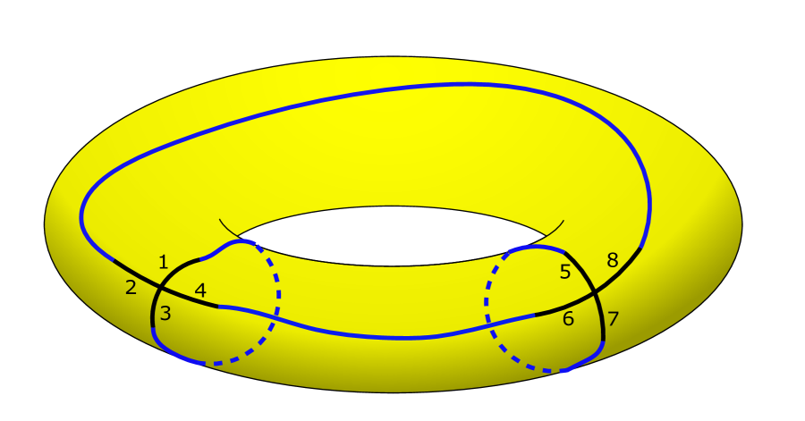
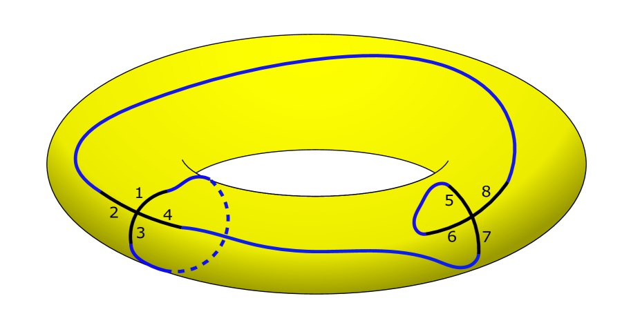
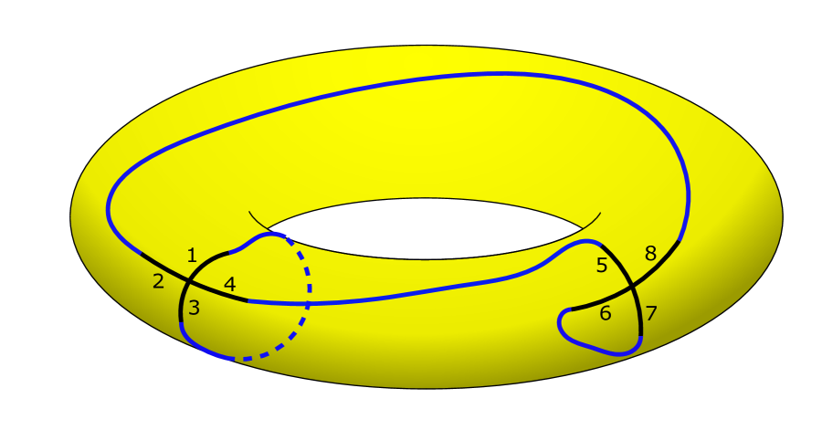
Figure 19. All three labeled connected 4-valent graphs with two vertices, where $e_{1}\leftrightarrow e_{3}$ & $e_{2}\leftrightarrow e_{8}$. Identically, for each of the cases $e_{1}\leftrightarrow e_{3}$ & $e_{2}\leftrightarrow e_{5}$, $e_{1}\leftrightarrow e_{3}$ & $e_{2}\leftrightarrow e_{7}$, and $e_{1}\leftrightarrow e_{3}$ & $e_{2}\leftrightarrow e_{6}$ there are three distinct graphs. Thus there exists $4\cdot 3=12$ distinct graphs with two vertices and $e_{1}\leftrightarrow e_{3}$ realizable on the torus.

It is easy to verify the first two members of (7.1). Consider a labeled 4-valent graph with a single vertex $v$. label the edges emanating from $v$ in a counterclockwise way by $e_{1},e_{2},e_{3},$ and $e_{4}$. For the simplicity of the Figures 16, 17, 18, 19, and 20 an edge $e_{k}$ will be simply denoted by $k$ on the graphs. It is clear that there are two ways to make a desired graph on the sphere in which one connects the adjacent edges ($\mathscr{N}_{1}(0)=2$). The graph in which the opposite edges are connected can not be realized on the sphere, but can be realized on the torus($\mathscr{N}_{1}(1)=1$).

Now we justify the third member of (7.1). Label the vertices by $v_{1}$ and $v_{2}$. Label the edges emanating from $v_{1}$ in a counterclockwise way by $e_{1},e_{2},e_{3},e_{4}$, and label the edges emanating from $v_{2}$ in a counterclockwise way by $e_{5},e_{6},e_{7},e_{8}$. When $e_{j}$ connects to $e_{k}$ we use the notation $e_{j}\leftrightarrow e_{k}$.

We exhaust all possibilities for which 4-valent connected labeled graphs with two vertices can be realized on the sphere. Let us start with $e_{1}$. This edge can be connected to any other labeled edge except for $e_{3}$, because obviously if these edges are connected then either $e_{2}$ or $e_{4}$ would have no destination. Now we show that $e_{1}$ can be connected to $e_{2}$ or $e_{4}$ in eight distinct graphs, while it can be connected to either $e_{5},e_{6},e_{7},$ or $e_{8}$ in five distinct graphs, which confirms that $\mathscr{N}_{2}(0)=2\cdot 8+4\cdot 5=36$. Figure 16 shows all eight connected labeled 4-valent graphs with two vertices on the sphere with a connection between $e_{1}$ and $e_{2}$, while Figure 17 shows all five connected labeled 4-valent graphs with two vertices on the sphere with a connection between $e_{1}$ and $e_{6}$.

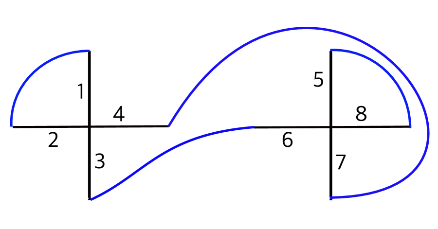
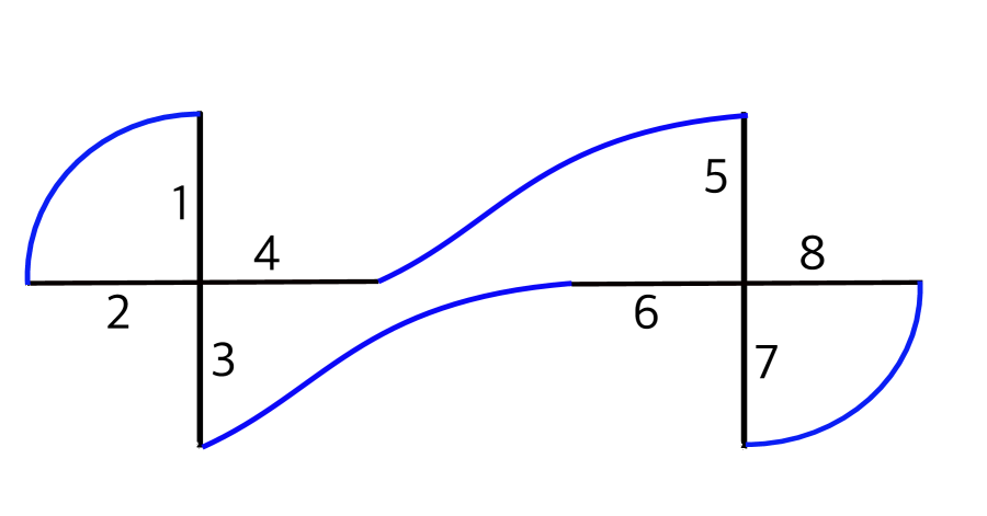
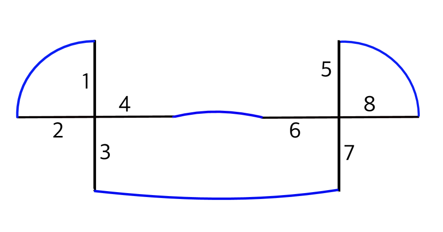
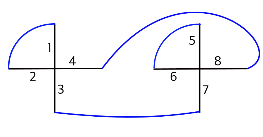
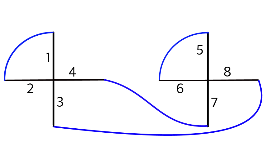
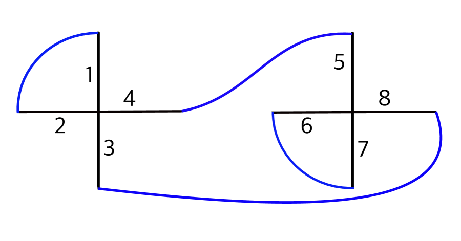
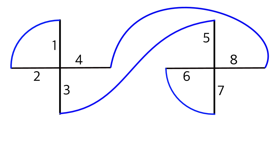
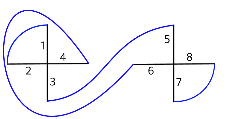
Figure 16. All eight labeled connected 4-valent graphs with two vertices, where $e_{1}$ connects to $e_{2}$ and realizable on the sphere. Identically, for the case where $e_{1}$ connects to $e_{4}$, there are also eight distinct graphs. For the simplicity of the Figures 16, 17, 18, 19, and 20 an edge $e_{k}$ will be simply denoted by $k$ on the graphs.

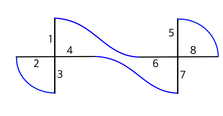
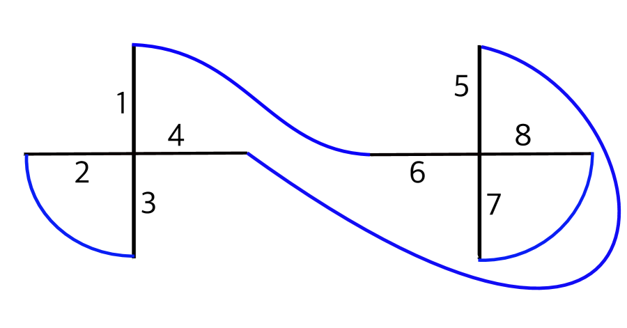
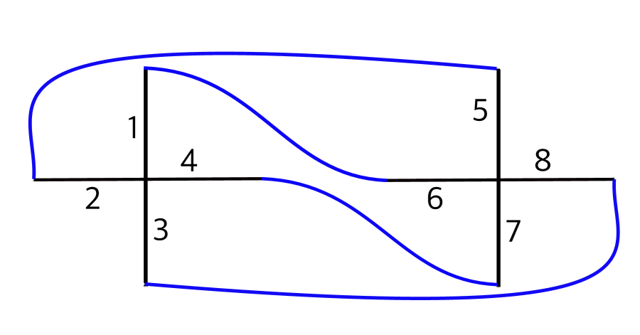
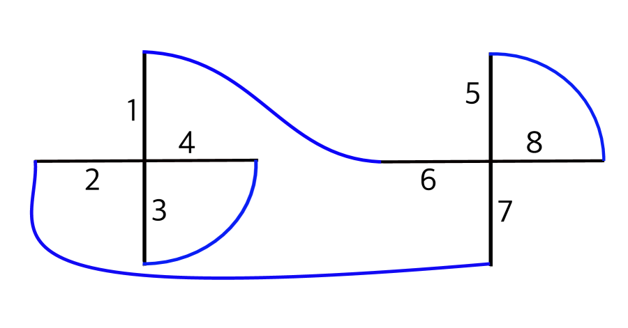
Figure 17. All five labeled connected 4-valent graphs with two vertices, where $e_{1}$ connects to $e_{6}$ and realizable on the sphere. Identically, for each of the cases where $e_{1}$ connects to $e_{5}$, $e_{7}$, or $e_{8}$, there are also five distinct graphs. this Figure together with Figure 16 confirm that $\mathscr{N}_{2}(0)=2\cdot 8+4\cdot 5=36$.

Now we try to justify that $\mathscr{N}_{2}(1)=60$. Notice that there are three distinct graphs if one enforces two pairwise connections. Since we have already realized two graphs with $e_{1}\leftrightarrow e_{2}$ and $e_{3}\leftrightarrow e_{6}$ on the sphere (see the first two graphs in Figure 16) there is only one remaining graph with $e_{1}\leftrightarrow e_{2}$ and $e_{3}\leftrightarrow e_{6}$ to be realized on the torus. Similarly, there is one graph left to be realized on the torus with the specifications: 1) $e_{1}\leftrightarrow e_{2}$ and $e_{3}\leftrightarrow e_{7}$ , 2) $e_{1}\leftrightarrow e_{2}$ and $e_{3}\leftrightarrow e_{8}$ , and 3) $e_{1}\leftrightarrow e_{2}$ and $e_{3}\leftrightarrow e_{5}$. Figure 18 shows all graphs with $e_{1}\leftrightarrow e_{2}$ which can be realized on the torus but not on the sphere.

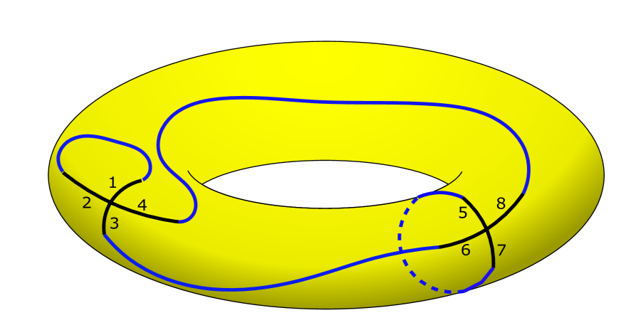
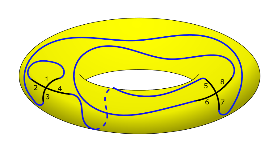
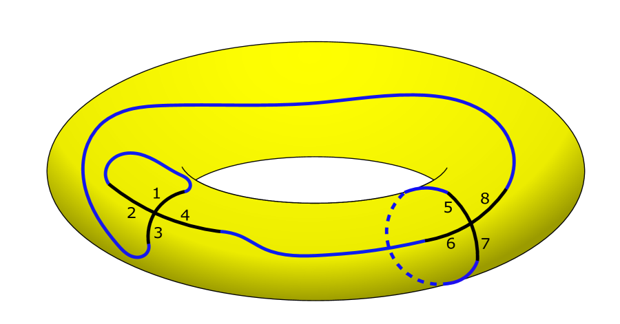
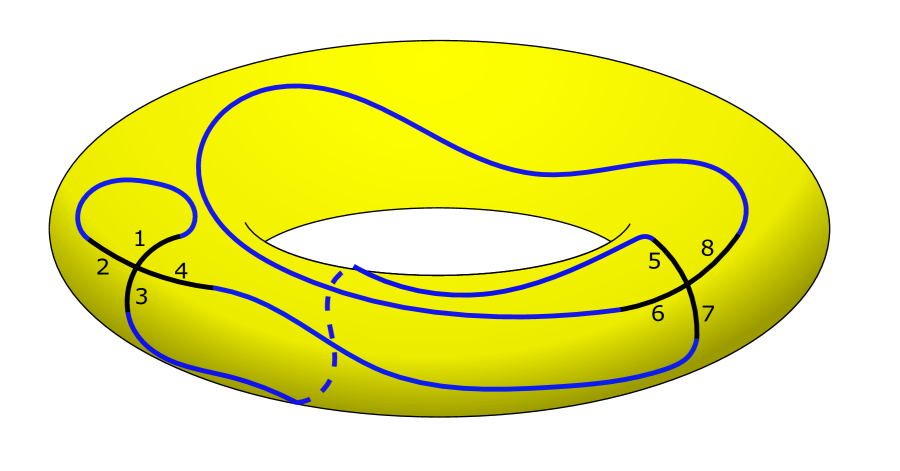
Figure 18. All four labeled connected 4-valent graphs with two vertices, where $e_{1}$ connects to $e_{2}$ which are not realizable on the sphere(compare with Figure 16). Identically, for the case where $e_{1}$ connects to $e_{4}$, there are also four distinct graphs.

In Figure 17 we have already realized two graphs with $e_{1}\leftrightarrow e_{6}$ & $e_{2}\leftrightarrow e_{3}$, two graphs with $e_{1}\leftrightarrow e_{6}$ & $e_{2}\leftrightarrow e_{5}$, and only one graph with $e_{1}\leftrightarrow e_{6}$ & $e_{2}\leftrightarrow e_{7}$. So there remains one graph with $e_{1}\leftrightarrow e_{6}$ & $e_{2}\leftrightarrow e_{3}$, one graph with $e_{1}\leftrightarrow e_{6}$ & $e_{2}\leftrightarrow e_{5}$, and two graphs with $e_{1}\leftrightarrow e_{6}$ & $e_{2}\leftrightarrow e_{7}$ to be realized on the torus (See the first four graphs in Figure 20). Although no graphs with $e_{1}\leftrightarrow e_{6}$ & $e_{2}\leftrightarrow e_{8}$, and no graphs with $e_{1}\leftrightarrow e_{6}$ & $e_{2}\leftrightarrow e_{4}$ could be realized on the sphere, one can check that all six such graphs could indeed be realized on the torus as shown in the last six graphs in Figure 20. In total, this gives 10 distinct graphs with $e_{1}\leftrightarrow e_{6}$ which can not be realized on the sphere but can be realized on the torus. Identically, for each one of the cases $e_{1}\leftrightarrow e_{5}$, $e_{1}\leftrightarrow e_{7}$, and $e_{1}\leftrightarrow e_{8}$ there also exist 10 distinct graphs that can not be realized on the sphere but can be realized on the torus. Thus far we have obtained $2\cdot 4+4\cdot 10=48$ distinct graphs with two vertices that can not be realized on the sphere but can be realized on the torus based on Figures 18 and 20. The only remaining case to focus on is the number of graphs with two vertices and $e_{1}\leftrightarrow e_{3}$ realizable on the torus (notice that $e_{1}\leftrightarrow e_{3}$ is not possible on the sphere). But this is now obvious as we describe now: Fix $e_{1}\leftrightarrow e_{3}$ and any of the four possible destinations $e_{5},e_{6},e_{7},$ or $e_{8}$ (Notice that $e_{4}$ can not be a destination for $e_{2}$ as it renders the graph disconnected). As described earlier, there are three distinct graphs with two enforced pairwise edge connections. Thus there exists $4\cdot 3=12$ distinct graphs with two vertices and $e_{1}\leftrightarrow e_{3}$ which can not be realized on the sphere but can be realized on the torus. This finishes our justification for $\mathscr{N}_{2}(1)=48+12=60$.

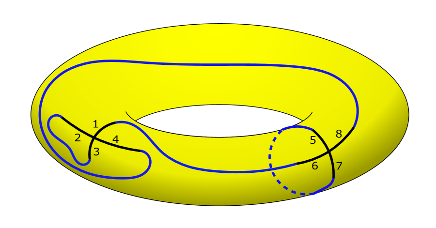
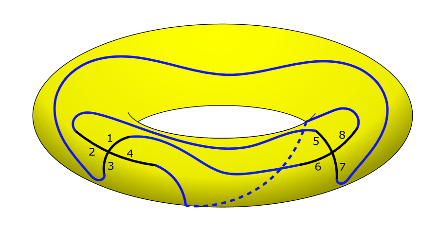
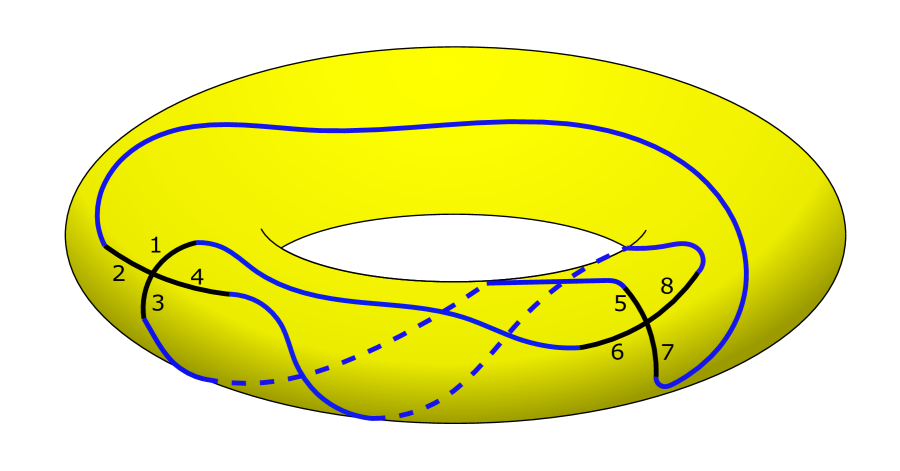
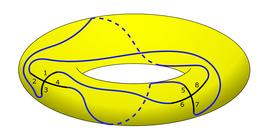
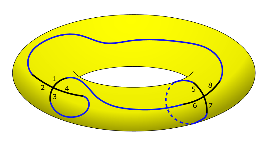
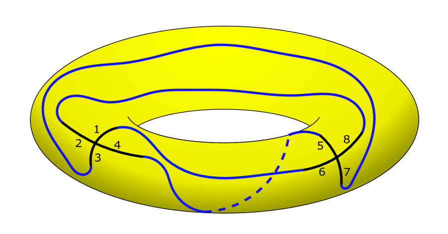
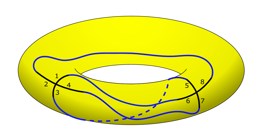
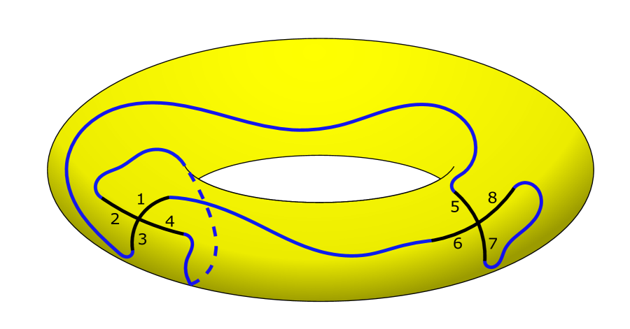
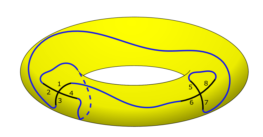
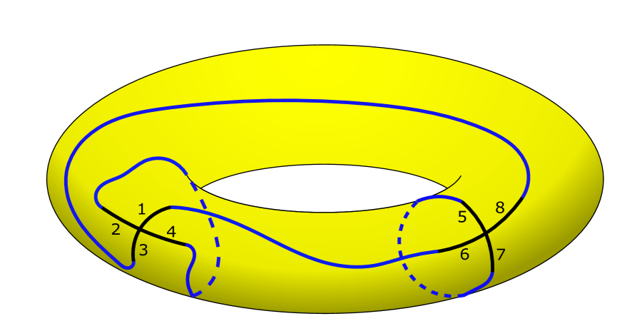
Figure 20. All ten labeled connected 4-valent graphs with two vertices, where $e_{1}$ connects to $e_{6}$ which are not realizable on the sphere(compare with Figure 17). Identically, for each one of the cases $e_{1}\leftrightarrow e_{5}$, $e_{1}\leftrightarrow e_{7}$, and $e_{1}\leftrightarrow e_{8}$ there also exist 10 distinct graphs. This means that there are totally 40 distinct graphs, not realizable on the sphere, where $e_{1}$ connects to one of the edges emanating from $v_{2}$.

References

- [BBG+22] Marco Bertola, Pavel Bleher, Roozbeh Gharakhloo, Kenneth T-R McLaughlin, and Alexander Tovbis. Openness of regular regimes of complex random matrix models. arXiv:2203.11348, 2022.
- [BC86] Edward A. Bender and E. Rodney Canfield. The asymptotic number of rooted maps on a surface. J. Combin. Theory Ser. A, 43(2):244–257, 1986.
- [BD12] Pavel Bleher and Alfredo Deaño. Topological Expansion in the Cubic Random Matrix Model. International Mathematics Research Notices, 2013(12):2699–2755, 05 2012.
- [BDJ99] Jinho Baik, Percy Deift, and Kurt Johansson. On the distribution of the length of the longest increasing subsequence of random permutations. J. Amer. Math. Soc., 12(4):1119–1178, 1999.
- [BDn16] Pavel Bleher and Alfredo Deaño. Painlevé I double scaling limit in the cubic random matrix model. Random Matrices Theory Appl., 5(2):1650004, 58, 2016.
- [BDY17] Pavel Bleher, Alfredo Deaño, and Maxim Yattselev. Topological expansion in the complex cubic log–gas model: One-cut case. Journal of Statistical Physics, 166(3):784–827, 2017.
- [Ber11] Marco Bertola. Boutroux curves with external field: equilibrium measures without a variational problem. Anal. Math. Phys., 1(2-3):167–211, 2011.
- [Bes79] Daniel Bessis. A new method in the combinatorics of the topological expansion. Comm. Math. Phys., 69(2):147–163, 1979.
- [BG13] Gaëtan Borot and Alice Guionnet. Asymptotic expansion of matrix models in the one-cut regime. Comm. Math. Phys., 317(2):447–483, 2013.
- [BGR08] Edward A. Bender, Zhicheng Gao, and L. Bruce Richmond. The map asymptotics constant . Electron. J. Combin., 15(1):Research paper 51, 8, 2008.
- [BI99] Pavel Bleher and Alexander Its. Semiclassical asymptotics of orthogonal polynomials, Riemann-Hilbert problem, and universality in the matrix model. Ann. of Math. (2), 150(1):185–266, 1999.
- [BI03] Pavel Bleher and Alexander Its. Double scaling limit in the random matrix model: the Riemann-Hilbert approach. Comm. Pure Appl. Math., 56(4):433–516, 2003.
- [BI05] Pavel Bleher and Alexander Its. Asymptotics of the partition function of a random matrix model. Annales de l’Institut Fourier, 55(6):1943–2000, 2005.
- [BIPZ78] Édouard. Brézin, Claude. Itzykson, Giorgio. Parisi, and Jean-Bernard. Zuber. Planar diagrams. Comm. Math. Phys., 59(1):35–51, 1978.
- [BIZ80] Daniel Bessis, Claude Itzykson, and Jean-Bernard Zuber. Quantum field theory techniques in graphical enumeration. Advances in Applied Mathematics, 1(2):109 – 157, 1980.
- [BL14] Pavel Bleher and Karl Liechty. Random matrices and the six-vertex model, volume 32 of CRM Monograph Series. American Mathematical Society, Providence, RI, 2014.
- [Bou13] P. Boutroux. Recherches sur les transcendantes de M. Painlevé et l’étude asymptotique des équations différentielles du second ordre. Ann. Sci. École Norm. Sup. (3), 30:255–375, 1913.
- [BT15] Marco Bertola and Alexander Tovbis. Asymptotics of orthogonal polynomials with complex varying quartic weight: global structure, critical point behavior and the first Painlevé equation. Constr. Approx., 41(3):529–587, 2015.
- [BT16] Marco Bertola and Alexander Tovbis. On asymptotic regimes of orthogonal polynomials with complex varying quartic exponential weight. SIGMA Symmetry Integrability Geom. Methods Appl., 12:Paper No. 118, 50, 2016.
- [CCH15] Ovidiu. Costin, Rodica D. Costin, and Min. Huang. Tronquée solutions of the Painlevé equation PI. Constr. Approx., 41(3):467–494, 2015.
- [CG21] Christophe Charlier and Roozbeh Gharakhloo. Asymptotics of Hankel determinants with a Laguerre-type or Jacobi-type potential and Fisher-Hartwig singularities. Adv. Math., 383:Paper No. 107672, 69, 2021.
- [Cha18] Christophe Charlier. Asymptotics of Hankel determinants with a one-cut regular potential and Fisher-Hartwig singularities. Int. Math. Res. Not., 62:pp. https://doi.org/10.1093/imrn/rny009, 2018.
- [Dav85] François David. Planar diagrams, two-dimensional lattice gravity and surface models. Nuclear Phys. B, 257(1):45–58, 1985.
- [Dav91] François David. Phases of the large-n matrix model and non-perturbative effects in 2d gravity. Nuclear Physics B, 348(3):507–524, 1991.
- [DFGZJ95] P. Di Francesco, P. Ginsparg, and J. Zinn-Justin. D gravity and random matrices. Phys. Rep., 254(1-2):133, 1995.
- [DK06] M. Duits and A. B. J. Kuijlaars. Painlevé I asymptotics for orthogonal polynomials with respect to a varying quartic weight. Nonlinearity, 19(10):2211–2245, 2006.
- [EM03] Nicholas M. Ercolani and Kenneth. D. T-R. McLaughlin. Asymptotics of the partition function for random matrices via Riemann-Hilbert techniques and applications to graphical enumeration. Int. Math. Res. Not., (14):755–820, 2003.
- [EMP08] Nicholas. M. Ercolani, Kenneth D. T-R. McLaughlin, and Virgil U. Pierce. Random matrices, graphical enumeration and the continuum limit of toda lattices. Communications in Mathematical Physics, 278(1):31–81, 2008.
- [Erc11] Nicholas. M. Ercolani. Caustics, counting maps and semi-classical asymptotics. Nonlinearity, 24(2):481–526, 2011.
- [Erc14] Nicholas M. Ercolani. Conservation laws of random matrix theory. In Random matrix theory, interacting particle systems, and integrable systems, volume 65 of Math. Sci. Res. Inst. Publ., pages 163–197. Cambridge Univ. Press, New York, 2014.
- [EW21] Nicholas M. Ercolani and Patrick Waters. Relating random matrix map enumeration to a universal symbol calculus for recurrence operators in terms of Bessel-Appell polynomials. arXiv:1907.08026, 2021.
- [FIK92] Athanassios S. Fokas, Alexander R. Its, and Alexander V. Kitaev. The isomonodromy approach to matrix models in D quantum gravity. Comm. Math. Phys., 147(2):395–430, 1992.
- [FIKN06] Athanassios S. Fokas, Alexander R. Its, Andrei A. Kapaev, and Victor Yu. Novokshenov. Painlevé transcendents, volume 128 of Mathematical Surveys and Monographs. American Mathematical Society, Providence, RI, 2006. The Riemann-Hilbert approach.
- [Gao91] Zhicheng Gao. The number of rooted triangular maps on a surface. J. Combin. Theory Ser. B, 52(2):236–249, 1991.
- [Gao93] Zhicheng Gao. A pattern for the asymptotic number of rooted maps on surfaces. J. Combin. Theory Ser. A, 64(2):246–264, 1993.
- [GLMn08] Stavros Garoufalidis, Thang T. Q. Lê, and Marcos Mariño. Analyticity of the free energy of a closed 3-manifold. SIGMA Symmetry Integrability Geom. Methods Appl., 4:Paper 080, 20, 2008.
- [Kap04] A. A. Kapaev. Quasi-linear stokes phenomenon for the Painlevé first equation. J. Phys. A, 37(46):11149–11167, 2004.
- [Kaz85] Vladimir A. Kazakov. Bilocal regularization of models of random surfaces. Physics Letters B, 150(4):282–284, 1985.
- [KM01] Arno B. J. Kuijlaars and Kenneth T.-R. McLaughlin. Riemann-Hilbert analysis for Laguerre polynomials with large negative parameter. Comput. Methods Funct. Theory, 1(1, [On table of contents: 2002]):205–233, 2001.
- [KM04] Arno B. J. Kuijlaars and Kenneth T.-R. McLaughlin. Asymptotic zero behavior of Laguerre polynomials with negative parameter. Constr. Approx., 20(4):497–523, 2004.
- [KS15] Arno B. J. Kuijlaars and Guilherme L. F. Silva. S-curves in polynomial external fields. J. Approx. Theory, 191:1–37, 2015.
- [MFR11] Andrei Martínez-Finkelshtein and Evguenii A. Rakhmanov. Critical measures, quadratic differentials, and weak limits of zeros of Stieltjes polynomials. Comm. Math. Phys., 302(1):53–111, 2011.
- [Rak12] Evguenii A. Rakhmanov. Orthogonal polynomials and -curves. In Recent advances in orthogonal polynomials, special functions, and their applications, volume 578 of Contemp. Math., pages 195–239. Amer. Math. Soc., Providence, RI, 2012.
- [ST97] Edward B. Saff and Vilmos Totik. Logarithmic potentials with external fields, volume 316 of Grundlehren der mathematischen Wissenschaften [Fundamental Principles of Mathematical Sciences]. Springer-Verlag, Berlin, 1997. Appendix B by Thomas Bloom.
- [Str84] Kurt Strebel. Quadratic differentials, volume 5 of Ergebnisse der Mathematik und ihrer Grenzgebiete (3) [Results in Mathematics and Related Areas (3)]. Springer-Verlag, Berlin, 1984.
- [tH74] Gerard ’t Hooft. A planar diagram theory for strong interactions. Nuclear Physics B, 72(3):461–473, 1974.
- [Wit91] Edward Witten. Two-dimensional gravity and intersection theory on moduli space. In Surveys in differential geometry (Cambridge, MA, 1990), pages 243–310. Lehigh Univ., Bethlehem, PA, 1991.
- [Zvo97] Alexander K. Zvonkin. Matrix integrals and map enumeration: an accessible introduction. volume 26, pages 281–304. 1997. Combinatorics and physics (Marseilles, 1995).