Numerical method to solve impulse control problems for partially observed piecewise deterministic Markov processes

Abstract

Designing efficient and rigorous numerical methods for sequential decision-making under uncertainty is a difficult problem that arises in many applications frameworks. In this paper we focus on the numerical solution of a subclass of impulse control problem for piecewise deterministic Markov process (PDMP) when the jump times are hidden. We first state the problem as a partially observed Markov decision process (POMDP) on a continuous state space and with controlled transition kernels corresponding to some specific skeleton chains of the PDMP. Then we proceed to build a numerically tractable approximation of the POMDP by tailor-made discretizations of the state spaces. The main difficulty in evaluating the discretization error come from the possible random or boundary jumps of the PDMP between consecutive epochs of the POMDP and requires special care. Finally we extensively discuss the practical construction of discretization grids and illustrate our method on simulations.

1 Introduction

A large number of problems in science, including resource management, financial portfolio management, medical treatment design to name just a few, can be characterized as sequential decision-making problems under uncertainty. In such problems, an agent interacts with a dynamic, stochastic, and incompletely known process, with the goal of finding an action-selection strategy that optimises some performance measure over several time steps. In optimal stopping problems, for instance when the agent has to decide when to replace some component of a production chain before full deterioration, the policy typically does not influence the underlying process until replacement when the process starts again with the same dynamics. However in many decision-making problems an important aspect is the effect of the agent’s policy on the data collection; different policies naturally yielding different behaviors of the process at hand.

In this paper we focus on the numerical solution of a subclass of impulse control problem for Piecewise Deterministic Markov Process (PDMP) when the process is partially observed, in the hard case when jump times are hidden. PDMPs are continuous time processes with hybrid state space: they can have both discrete and Euclidean variables. The dynamics of a PDMP is determined by three local characteristics: the flow, the jump intensity and the Markov jump kernel, see [10]. Between jumps, trajectories follow the deterministic flow. The frequency of jumps is determined by the intensity or by reaching boundaries of the state space, and the post-jump location is selected by the Markov kernel.

General impulse control for PDMPs allows the controller to act on the process dynamics by choosing intervention dates and new states to restart from at each intervention. This family of problems was first studied by Costa and Davis in [9]. It has received a lot of attention since, see e.g. [1, 8, 14, 15], and was further extended for instance in [16, 17]. In these papers, the authors define a rigorous mathematical framework to state such control problem and establish some optimality equations such as dynamic programming equations for the value function. Numerical methods to compute an approximation of the value function and an $\epsilon$-optimal policy are also briefly or extensively described for instance in [9, 12, 13]. They rely on discretization of the state space, either with direct cartesian grids or with dynamic grids obtained from simulations of the inter-jump-time-post-jump-location discrete time Markov chain embedded in the PDMP.

In all the papers cited above, the process is supposed to be perfectly observed at all times. However in most real-life applications continuous measurements are not available, and measures may be corrupted by noise. Designing efficient and mathematically sound approximation methods to solve continuous time and continuous state space impulse control problems under partial observation is very challenging, especially for processes with jumps such as PDMPs. Relevant literature is scarce. One can mention [2] or [4] (in the special easier case of optimal stopping) where the position of the process is observed through noise, but the jump times are perfectly observed, so that the properties of the inter-jump-time-post-jump-location chain can still be fully exploited. Another related recent work is [5] where the author studies an optimal control problem for pure jump processes (corresponding to PDMPs with contant flow) under partial observations. However, they consider continuous control instead of impulse control and the observations are not corrupted by noise.

A first step toward solving the impulse control problem for PDMPs under partial and noisy observations and hidden jump times was made by the authors in [6] in the special easier case of optimal stopping. They have shown that when trajectories of the process can be simulated, a double discretization allows to approximate the value function with general error bounds, and provides a candidate policy with excellent performance. In this paper, we address a more general class of impulse control problems under partial observations where decisions do influence both the data collection and the dynamics of the process. More specifically, we focus on a sub class of impulse control problems with three specificities. First, the lapse between interventions can only take a finite number of values. Second, observations are collected at intervention times and corrupted by noise. Third, interventions only act on the discrete variables. In this setting, the impulse control problem can be stated as a partially observed Markov decision process (POMDP) and this is the first main contribution of this paper. This POMDP is in discrete time, with epochs corresponding to intervention dates, however the state space is not discrete, and becomes infinite dimensional when turned into the corresponding fully observed Markov decision process (MDP) for the filter on the belief space, see e.g. [3]. While such MDPs have theoretical exact optimal solutions, they are numerically untractable. Our second main contribution is to propose and prove the convergence of an algorithm to approximate the value fonction and explicitly build a policy close to optimality. Our approach is based on tailor-made discretizations of the state spaces taking into account two major difficulties. First, the state space may have numerous active boundaries that trigger jumps when reached and make the operators under study only locally regular. Second, the combinatorics associated to the possible decisions is too large to explore the whole belief space through simulations. Our third main contribution is to extensively discuss the practical construction of the discretization grids, which is no easy problem. Our results are illustrated by simulations on an example of medical treatment optimization for cancer patients.

The paper is organized as follows. In section 2 we state our optimization problem and turn it into a POMPD. In section 3 we give our resolution strategy and our main assumptions. The construction of the approximate value function and policy is detailed in section 4. Experimental results and discussion of the practical construction of discretization grids are provided in section 5. Finally section 6 provides a short conclusion. The main proofs are postponed to the appendix as well as details and specifications of the model used for the simulation study.

2 Problem statement

We start with specifying the special class of impulse control problem for PDMPs we are focusing on, then we show how our control problem can be expressed as a POMDP.

2.1 Impulse control for hidden PDMPs

Let us first define the class of controlled PDMPs we consider. Let $\mathcal{M}=L\times M$ be a two-dimensional finite set. We will call regimes or modes its elements. We use a product set to distinguish between modes in $L$ that can be controller chosen and modes in $M$ that cannot. For all regime $(\ell,m)$ in $\mathcal{M}$, let $E_{m}^{\ell}$ be an open subset of $\mathbb{R}^{d}$ endowed with a norm $\|\cdot\|$. Set $E=\{(\ell,m,\mathtt{x}),\ell\in L,m\in M,\mathtt{x}\in E_{m}^{\ell}\}$, and $E^{\ell}=\{(m,\mathtt{x}),m\in M,\mathtt{x}\in E_{m}^{\ell}\}$ for all $\ell\in L$. A PDMP on the state space $E$ is determined by three local characteristics:

• the flow $\boldsymbol{\Phi}(x,t)=(\ell,m,\Phi_{m}^{\ell}(\mathtt{x},t))$ for all $x=(\ell,m,\mathtt{x})$ in $E$ and $t\geq 0$, where $\Phi_{m}^{\ell}:\mathbb{R}^{d}\times\mathbb{R}_{+}\rightarrow\mathbb{R}^{d}$ is continuous and satisfies a semi-group property $\Phi_{m}^{\ell}(\cdot,t+s)=\Phi_{m}^{\ell}(\Phi_{m}^{\ell}(\cdot,t),s)$, for all $t,s\in\mathbb{R}_{+}$. It describes the deterministic trajectory between jumps. Let $\boldsymbol{t}^{*}(x)=t_{m}^{*\ell}(\mathtt{x})$ be the deterministic time the flow takes to reach the boundary of $E$ when it starts from $x=(\ell,m,\mathtt{x})$:

  $$\boldsymbol{t}^{*}(x)=\inf\{t>0:\Phi_{m}^{\ell}(\mathtt{x},t)\in\partial E_{m}^{\ell}\}.$$

• the jump intensity $\boldsymbol{\lambda}(x)=\lambda_{m}^{\ell}(\mathtt{x})$ for all $x=(\ell,m,\mathtt{x})$ in $E$, where $\lambda_{m}^{\ell}:\bar{E}_{m}^{\ell}\rightarrow\mathbb{R}^{+}$ is a measurable function such that for any $x=(\ell,m,\mathtt{x})$ in $E$, there exists $\epsilon>0$ such that

  $$\int_{0}^{\epsilon}\lambda_{m}^{\ell}(\Phi_{m}^{\ell}(\mathtt{x},t))dt<+\infty.$$

  For all $x=(\ell,m,\mathtt{x})$ in $E$ and $t\in[0;\boldsymbol{t}^{*}(x)]$, set

  $$\boldsymbol{\Lambda}(x,t) =\Lambda_{m}^{\ell}(\mathtt{x},t)=\int_{0}^{t}\lambda_{m}^{\ell}(\Phi_{m}^{\ell}(\mathtt{x},s))ds.$$

• the Markov kernel $\boldsymbol{Q}$ on $(\mathcal{B}(\bar{E}),\bar{E})$ represents the transition measure of the process and allows to select the new location after each jump. It satisfies for all $x\in\bar{E}$, $\boldsymbol{Q}(\{x\}\cup\partial E|x)=0$. We also write $Q_{m}^{\ell}(\cdot|\mathtt{x})=\boldsymbol{Q}(\cdot|x)$ for all $x=(\ell,m,\mathtt{x})\in E$ and add the additional constraint that $Q$ cannot change the value of $\ell$, as $\ell$ is intended to be controller-chosen, i.e. $Q_{m}^{\ell}$ sends $E^{\ell}$ onto itself.

The formal probabilistic apparatus necessary to precisely define controlled trajectories and to formally state the impulse control problem is rather cumbersome, and will not be used in the sequel. Therefore, for the sake of simplicity, we only present an informal description of the construction of controlled trajectories. The interested reader is referred to [9], [11, section 54] or [16] for a formal setting. Our optimization problem will be rigorously stated as a POMDP in section 2.2.

We consider a finite horizon problem. Let $H>0$ be the optimization horizon, $\delta>0$ a fixed minimal lapse such that $N=H/\delta$ is an integer. Note that $\delta$ is not supposed to be small. A general impulse strategy $\mathcal{S}=(\ell_{n},r_{n})_{0\leq n\leq N-1}$ is a sequence of non-anticipative $E$-valued random variables on a measurable space $(\Omega,\mathcal{F})$ and of non-anticipative intervention lapses. In this work, we only consider a subclass of strategies where $\ell_{n}$ takes values in $L$ and $r_{n}$ is a multiple of $\delta$: $r_{n}\in\mathbb{T}$ where $\mathbb{T}$ is a subset of $\delta^{1:N}=\{\delta,2\delta,\ldots,N\delta\}$ that contains $\delta$. This means that on the one hand, the controller can only act on the process by changing its regime, i.e. by selecting the local characteristics to be applied until the next intervention, and on the other hand the lapse between consecutive interventions belongs to the finite set $\mathbb{T}$. The trajectories of the PDMP controlled by strategy $\mathcal{S}$ are constructed recursively between intervention dates $\tau_{n}$ (defined recursively by $\tau_{0}=0$ and $\tau_{n+1}=\tau_{n}+r_{n}$) as described in algorithm 1.

Algorithm 1 Simulation of a trajectory of a controlled PDMP between interventions $n$ and $n+1$ from state $x_{n}=(\ell_{n},m_{n},\mathtt{x}_{n})$

1:  $s\leftarrow 0$

2:  $\ell\leftarrow\ell_{n},m\leftarrow m_{n},\mathtt{x}\leftarrow\mathtt{x}_{n},x\leftarrow(\ell,m,\mathtt{x})$

3:  while $s<r_{n}$ do

4:     $S\sim\lambda_{m}^{\ell}(\mathtt{x})$

5:     $S\leftarrow\min\{S,\boldsymbol{t}^{*}(x_{n})\}$

6:     $X_{\tau_{n}+t}\leftarrow\boldsymbol{\Phi}(x,t)$ for $0\leq t\leq\min\{(s+S),r_{n}\}$

7:     $\mathtt{x}\leftarrow\Phi_{m}^{\ell}(\mathtt{x},s)$

8:     if $s+S\leq r_{n}$ then

9:        $s\leftarrow s+S$

10:        $(\ell,m^{\prime},\mathtt{x}^{\prime})\sim Q_{m}^{\ell}(\cdot|\mathtt{x})$

11:        $m\leftarrow m^{\prime},\mathtt{x}\leftarrow\mathtt{x}^{\prime},x\leftarrow(\ell,m,\mathtt{x})$

12:     end if

13:  end while

In Line 5 of algorithm 1, $S\sim\lambda_{m}^{\ell}(\mathtt{x})$ means that $S$ has the survival function

$$\mathbb{P}_{x}(S>t)=e^{-\int_{0}^{t}\lambda_{m}^{\ell}(\Phi_{m}^{\ell}(\mathtt{x},s))ds}=e^{-\boldsymbol{\Lambda}(x,t)}.$$

As a boundary jump can also occur, the distribution of the next jump time $T$, starting from $x$ is given by the survival function

$$\mathbb{P}_{x}(T>t)=e^{-\int_{0}^{t}\lambda_{m}^{\ell}(\Phi_{m}^{\ell}(\mathtt{x},s))ds}\mathbbm{1}_{t<\boldsymbol{t}^{*}(x)}=e^{-\boldsymbol{\Lambda}(x,t)}\mathbbm{1}_{t<\boldsymbol{t}^{*}(x)}.$$

The strategy $\mathcal{S}$ induces a family of probability measures $\mathbb{P}^{\mathcal{S}}_{x}$, $x\in E$, on a suitable probability space $(\Omega,\mathcal{F})$. Associated to strategy $\mathcal{S}$, we define the following expected total cost for a process starting at $x\in E$

$$\mathcal{J}(\mathcal{S},x)=\mathbb{E}_{x}^{\mathcal{S}}\Bigl{[}\int_{0}^{H}c_{r}(X_{s})ds+\sum_{n=0}^{N-1}c_{i}({X}_{\tau_{n}},\ell_{n},r_{n})+c_{t}(X_{H})\Bigr{]},$$ (1)

where $\mathbb{E}_{x}^{\mathcal{S}}$ is the expectation with respect to $\mathbb{P}^{\mathcal{S}}_{x}$, $c_{r}$ is some running cost, $c_{i}$ some intervention cost and $c_{t}$ some terminal cost.

The last ingredient needed to state the optimisation problem is to define admissible strategies. Again, the rigorous definition will be given in section 2.2 in the framework of POMDPs. Informally, decisions can only be taken in view of some discrete-time noisy observations of the process, instead of the exact value of the process at all times. More specifically, we assume that

• observations are only available at decision times $\tau_{n}$,

• the controller-chosen regimes $\ell\in L$ are observed, the uncontrolled regimes $m\in M$ are hidden, except for some top event $m=\bar{m}$;

• the Euclidean variable is observed through noise: at time $\tau_{n}$, if the state of the process is $x=(\ell,m,\mathtt{x})$, controller receives observation $y_{n}=F(\mathtt{x})+\epsilon_{n}$ where $(\epsilon_{n})$ are real-valued independent and identically distributed random variables with density $f$ independent from the controlled PDMP. We further assume that the random variables $y_{n}$ take values in a compact interval $I$ of the real line.

Denote by $\mathbb{S}$ the set of all admissible strategies. Our aim is to compute an approximation of the value function

$$\mathcal{V}(x)=\inf_{\mathcal{S}\in\mathbb{S}}\mathcal{J}(\mathcal{S},x),$$

and explicitly construct a strategy close to optimality.

2.2 Partially observed Markov decision process

Finding a suitable rigorous way to state an impulse control problem for PDMPs with hidden jumps and under noisy observation is by no means straightforward, especially as regards defining admissible strategies, see e.g. [1] or [7, sec. 1.1]. This is our first main contribution in this paper. As decision dates are discrete, we use the framework of POMPDs to rigorously state our control problem. In the sequel, we drop the regime $\ell\in L$ from the state $x$ and include it in the action instead to better fit the standard POMDP notation. Denote $E_{m}=\cup_{\ell\in L}E_{m}^{\ell}$, $E_{<\bar{m}}=\cup_{m\neq\bar{m}}E_{m}$ and $E_{M}=\{(m,{\tt x}),m\in M,{\tt x}\in E_{m}\}$. Define on $E_{M}$ the following hybrid distance, for $x=(m,{\tt x})$ and $x^{\prime}=(m^{\prime},{\tt x}^{\prime})\in E_{M}$,

$$\|x-x^{\prime}\|=(\|{\tt x}-{\tt x}^{\prime}\|)\mathbbm{1}_{m=m^{\prime}}+\infty\mathbbm{1}_{m\neq m^{\prime}}.$$

Let $(\mathbb{X},\mathbb{A},\mathbb{K},R,c,C)$ be the POMPD with the following characteristics.

$\bullet$ The state space is $\mathbb{X}=\{\xi=(x,y,z,w)\in(E_{M}\times\mathbb{O});z=\mathbbm{1}_{\{x_{1}=\bar{m}\}}\}\cup\{\Delta\}$, with $\mathbb{O}=\{\gamma\in I\times\{0,1\}\times\delta^{1:N}\}$ the observation space. It gathers the values $X_{n}$ of the hidden PDMP at dates $\tau_{n}$ as well as the observation processes $Y_{n}$, and two additional observed variables $Z_{n}$ and $W_{n}$. Here, $Z_{n}$ is an indicator of being in mode $\bar{m}$ (hence at the top event) and $W_{n}$ is the time elapsed since the beginning. State $\Delta$ is a cemetery state where the process is sent after the horizon $H$ or mode $\bar{m}$ is reached.

$\bullet$ The action space is $\mathbb{A}=(L\times\mathbb{T})\cup\{\check{d}\}$, where $\check{d}$ is an empty decision that is taken when the horizon $H$ or mode $\bar{m}$ is reached. This purely technical decision sends the process to the cemetery state $\Delta$.

$\bullet$ The constraints set $\mathbb{K}\subset\mathbb{X}\times\mathbb{A}$ is such that its sections $\mathbb{K}(\xi)=\{d\in\mathbb{A};(\xi,d)\in\mathbb{K}\}$ satisfy $\mathbb{K}(\Delta)=\{\check{d}\}$ and $\mathbb{K}(x,y,z,w)=\mathbb{K}(z,w)$ for $(x,y,z,w)\in\mathbb{X}-\{\Delta\}$ as decisions are taken in view of the information from the observations only. In addition, one has

• $\mathbb{K}(0,w)=L\times(\mathbb{T}\cap\{\delta,2\delta,\dots,N\delta-w\})$ if $w\leq\delta(N-1)$, to force the last intervention to occur exactly at the horizon time $H$, unless mode $\bar{m}$ ($z=1$) has been reached,

• $\mathbb{K}(0,N\delta)=\mathbb{K}(1,w)=\check{d}$: no intervention is possible after the horizon or the top event has been reached.

Note that as $\delta\in\mathbb{T}$, the set $\mathbb{T}\cap\{\delta,2\delta,\dots,N\delta-w\}$ is never empty.

$\bullet$ The controlled transition kernels $R$ are defined as follows: for any bounded measurable function $g$ on $\mathbb{X}$, any $\xi\in\mathbb{X}$ and $d\in\mathbb{K}(\xi)$, one has

$$Rg(\xi,d) =g(\Delta),\quad\text{ if }d=\check{d},$$

$$Rg(\xi,d) =\int_{I}\int_{E_{<\bar{m}}}g(x^{\prime},y^{\prime},0,w+r)f(y^{\prime}-F(x^{\prime}))P(dx^{\prime}|x,d)dy^{\prime}$$

$$\quad+{\int_{E_{\bar{m}}}g(x^{\prime},0,1,w+r)P(dx^{\prime}|x,d)},\quad\text{ if }\xi=(x,y,0,w),\ d=(\ell,r)\neq\check{d},$$

$$Rg(\xi,d) =0,\quad\text{ otherwise,}$$

where $P(\cdot|x,d)$ is the distribution of $X_{r}$ conditionally to $X_{0}=x$ under regime $\ell$, if $d=(\ell,r)$. Its explicit analytical form is given in appendix A.

$\bullet$ The terminal cost function $C:\mathbb{X}\to\mathbb{R}_{+}$ satisfies $C(\Delta)=0$ and $C(x,y,z,w)=c_{t}(x)$ for $(x,y,z,w)\in\mathbb{X}-\{\Delta\}$ with $c_{t}(x)=c_{\bar{m}}$ if $x\in E_{\bar{m}}$,where $c_{\bar{m}}$ is a penalty for reaching the top value.

$\bullet$ The non-negative cost-per-stage function $c:\mathbb{K}\times\mathbb{X}\to\mathbb{R}_{+}$ satisfies $c(\Delta,\check{d},\cdot)=0$, $c(\xi,\check{d},\cdot)=C(\xi)$ and $c(\xi,d,\xi^{\prime})=c_{\bar{m}}$ if $x^{\prime}\in E_{\bar{m}}$. Ideally, to match eq. 1, for $d=(\ell,r)$ one should choose $c$ as

$$c(x,d)=\mathbb{E}_{x}^{\ell}\Bigl{[}\int_{0}^{r}c_{r}(X_{s})ds\Bigr{]}+c_{i}(x,d).$$

However, the integral part has no simple analytical expression and we choose some simpler proxys instead, see section 5.1.

$\bullet$ The optimisation horizon is finite and equals $N$ corresponding to date $N\delta=H$.

Classically, the sets of observable histories are defined recursively by $H_{0}=\mathbb{O}\cup\{\Delta\}$ and $H_{n}=H_{n-1}\times\mathbb{A}\times(\mathbb{O}\cup\{\Delta\})$. A decision rule at time $n$ is a measurable mapping $g_{n}:H_{n}\rightarrow\mathbb{A}$ such that $g_{n}(h_{n})\in\mathbb{K}(\gamma_{n})$ for all histories $h_{n}=(\gamma_{0},d_{0},\gamma_{1},d_{1},\ldots,\gamma_{n})$. A sequence $\pi=(g_{n})_{0:N-1}=(g_{0},\ldots,g_{n},\ldots,g_{N-1})$ where $g_{k}$ is a decision rule at time $k$ is called an admissible policy. Let $\Pi_{N}$ denote the set of all admissible policies. The controlled trajectory of the POMDP following policy $\pi=(g_{n})_{0:N-1}\in\Pi_{N}$ is defined recursively by $\Xi_{0}\in\mathbb{X}$ and for $0\leq n\leq N-1$,

• $A_{n}=g_{n}(\Xi_{n})$,

• $\Xi_{n+1}\sim R(\cdot|\Xi_{n},A_{n})$.

Note that the cemetery state $\Delta$ ensures that all trajectories have the same length $N$, even if they do not have the same number of actual decisions ($d\neq\check{d}$). Then one can define the total expected cost of policy $\pi\in\Pi_{N}$ starting at $\xi_{0}\in\mathbb{X}$ as

$$J_{\pi}(\xi_{0})=\mathbb{E}^{\pi}_{\xi_{0}}\left[\sum_{n=0}^{N-1}c(\Xi_{n},A_{n},\Xi_{n+1})+C(\Xi_{N})\right],$$

and our control problem corresponds to the optimisation problem

$$V(\xi_{0})=\inf_{\pi\in\Pi_{N}}J_{\pi}(\xi_{0}).$$

Now the problem is rigorously stated, our next aim is now to compute an approximation of the value function $V$ and explicitly construct a strategy close to optimality.

3 Resolution strategy and assumptions

Our second main contribution is to propose a numerical approach to (approximately) solve our POMDP. The first difficulty to solve our POMDP comes from the fact that it is partially observed. Thus our first step is to convert it into an equivalent fully observed MDP on a suitable belief space $\mathbb{X}^{\prime}$ by introducing a filter process. This is done in section 3.3. While dynamic programming equations hold true for the fully observed MDP and in theory provide the exact optimal strategy to the optimisation problem, there are two main difficulties to its practical resolution. On the one hand, the state space $\mathbb{X}^{\prime}$ is continuous and infinite-dimensional. And on the other hand the filter process is not simulatable, even for fixed policies, preventing the use of direct simulation-based discretization procedures.

Our approach to (approximately) solve the belief MDP is to construct a numerically tractable approximation of its value function based on discretizations of the dynamic programming equations. To obtain a finite-dimensional process and a simulatable approximation of the filter process, we first discretize the Euclidean part of the state space $E$ of the PDMP $(X_{t})$. Then we discretize the state space of the approximated filtered process in order to obtain a numerically tractable approximation. Finally, we obtain an explicit candidate policy by solving the resulting discretized approximation of the dynamic programming equations. This procedure is detailed in section 4.

In order to keep track of the discretization errors throughout the different steps described above, we need our transition kernels to be regular enough. Hence we start this section with stating the assumptions required on the parameters of the PDMP. The first set of assumptions stated in section 3.1 is not strictly necessary but is here to limit the combinatorics of possible jumps of the PDMP between consecutive epochs of the POMDP. The second set of assumptions in section 3.2 deals with regularity requirements and is necessary for our approach.

3.1 Simplifying assumptions on the dynamics of the PDMP

We make the following assumptions on the PDMP. Their aim is to limit the combinatorics of possible natural jumps between interventions, deal more easily with the boundary jumps, and obtain explicit forms for the transition kernel between two consecutive interventions. Although they are not strictly necessary for our approach to work, we believe they keep the exposition as simple as possible. First, we restrict the number of modes to create non trivial dynamics with limited enough combinatorics.

Assumption 3.1

The sets of regimes are $L=\{\emptyset,a,b\}$ and $M=\{0,1,2,3\}$.

We set $\bar{m}=3$ and in the sequel we write $E_{0:2}$ instead of $E_{<\bar{m}}$. Second, we consider a bounded one-dimensional Euclidean variable and add a counter of time since the last jump in order to encompass semi-Markov dynamics where the jump intensity is time dependent, instead of only state-dependent.

Assumption 3.2

The Euclidean variable is $\mathtt{x}=(\zeta,u)\in[\zeta_{0},D]\times[0,H]$, where $0<\zeta_{0}<D$ and $u$ is the time since the last jump.

Here we consider that $\zeta_{0}$ is some nominal value the process should stay close to, and $D$ is some non-return top value the process is trapped at when in mode $\bar{m}=3$. With a slight abuse of notation we will write $\Phi_{m}^{\ell}((\zeta,u),t)=(\Phi_{m}^{\ell}(\zeta,t),u+t)$. For $x=(m,\zeta,u)\in E_{M}$, we will also denote its coordinates $x_{1}=m$, $x_{2}=\zeta$ and $x_{3}=u$. Third, we specify monotonicity assumptions on the flow to be able to deal with boundaries easily.

Assumption 3.3

We make the following assumptions on $\Phi_{m}^{\ell}$

• in mode $m=0$ the flow is constant at the nominal value for any controller-specified $\ell\in L$: $\Phi_{0}^{\ell}(\zeta_{0},t)=\zeta_{0}$ for all $t\geq 0$;

• in modes $m=1$ and $m=2$, for any controller-specified $\ell\in L$, and any $\zeta\in(\zeta_{0},D)$, the application $t\mapsto\Phi_{m}^{\ell}(\zeta,t)$ is

  • non-increasing if $(m,\ell)\in\{(1,a),(2,b)\}$,

  • non-decreasing otherwise.

• in mode $m=3$ the flow is constant at the top value for any controller-specified $\ell\in L$: $\Phi_{3}^{\ell}(D,t)=D$ for all $t\geq 0$.

Basically, this means that in mode $m=0$, the process stays at the nominal value. In modes $m\in\{1,2\}$, if $\ell=\emptyset$, the Euclidean variable increases and may reach the top value. In both these modes, one of the controller-chosen modes is beneficial, in the sense that the process decreases and may reach the nominal value ($a$ for $m=1$ and $b$ for $m=2$) and the other one is neutral in the sense that the process keeps increasing ($b$ for $m=1$ and $a$ for $m=2$). We believe that this covers most interesting cases. In mode $m=3$ the process is trapped at the top value whatever the choice of the controller. Next, we restrict the number of natural jumps between interventions.

Assumption 3.4

For all $(m,\ell)\in\{(1,\emptyset),(2,\emptyset),(1,b),(2,a)\}$ and $r\in\mathbb{T}$, one has $t^{*\ell}_{m}(\zeta_{0})>r$ and $\lambda_{m}^{\ell}=0$. For all $\ell\in L$, $\lambda_{3}^{\ell}=0$

This is the strongest assumption. The first one prevents back-and-forth jumps between modes $1$ and $2$. The second one makes the top event absorbing. Finally, we consider that the Euclidean variable $\zeta$ is continuous and $u$ is set to $0$ by a natural jump as it represents the time since the last natural jump. In addition one can jump to mode $m=0$ only by reaching the bottom boundary $\zeta=\zeta_{0}$, and one can jump to mode $m=3$ only by reaching the top boundary $\zeta=D$.

Assumption 3.5

For $\zeta,\zeta^{\prime}\in[\zeta_{0},D]$ and $u\in[0,H]$ the jump kernel satisfies

$$Q_{m}^{\ell}(\{(m^{\prime},\zeta^{\prime},0)\}|\zeta,u) =Q_{m}^{\ell}(m^{\prime}|\zeta,u)\mathbbm{1}_{\zeta^{\prime}=\zeta},$$

$$Q_{m}^{\ell}(0|\zeta,u) =\mathbbm{1}_{\zeta=\zeta_{0}}\mathbbm{1}_{m\neq 0},$$

$$Q_{m}^{\ell}(3|\zeta,u) =\mathbbm{1}_{\zeta=D}\mathbbm{1}_{m\neq 3},$$

for all $(\ell,m)\in L\times M$ and $m^{\prime}\in M$.

3.2 Regularity assumptions

We start with regularity assumptions on the local characteristics of the PDMP.

Assumption 3.6

The jump intensity $\boldsymbol{\lambda}$ is Lipschitz continuous and bounded: there exist positive constants $[\lambda]$ and $\|\lambda\|$ such that for all $x$ and $x^{\prime}\in E_{M}$, $\ell\in L$, one has

$$|\boldsymbol{\lambda}(\ell,x)-\boldsymbol{\lambda}(\ell,x^{\prime})|\leq[\lambda]\|x-x^{\prime}\|,\qquad|\boldsymbol{\lambda}(\ell,x)|\leq\|\lambda\|.$$

Assumption 3.7

The flow $\boldsymbol{\Phi}$ is Lipschitz continuous: there exists a positive constant $[\Phi]$such that for all $x$ and $x^{\prime}\in E$, $\ell\in L$, and $t\in\mathbb{R}_{+}$ one has

$$|\boldsymbol{\Phi}(\ell,x,t)-\boldsymbol{\Phi}(\ell,x^{\prime},t)| \leq{[\Phi]\|x-x^{\prime}\|}.$$

The time to reach the boundary $\boldsymbol{t}^{*}$ is Lipschitz continuous: there exists a positive constant $[t^{*}]$ such that for all $m\in\{1,2\}$, $x,x^{\prime}\in E_{M}$ and $\ell\in L$, one has

$$|\boldsymbol{t}^{*}(\ell,x)-\boldsymbol{t}^{*}(\ell,x^{\prime})| \leq[t^{*}]\|x-x^{\prime}\|.$$

In addition, for all $m\in\{0,1,2\}$, $m^{\prime}\in\{1,2\}$ such that $m^{\prime}\neq m$, for all $\ell\in L$ and $\zeta\in(\zeta_{0},D)$ the mapping $t\mapsto t_{m^{\prime}}^{*\ell}(\Phi_{m}^{\ell}(\zeta,t))+t$ is a one-to-one correspondance and is Lipschitz continuous: there exist a positive constant $[S]$ such that if there exist $s=s(\zeta)$ and $s^{\prime}=s^{\prime}(\zeta^{\prime})$ in $(0,r)$ satisfying $t_{m^{\prime}}^{*\ell}(\Phi_{m}^{\ell}(\zeta,s))=r-s$ and $t_{m^{\prime}}^{*\ell}(\Phi_{m}^{\ell}(\zeta^{\prime},s^{\prime}))=r-s^{\prime}$, then one has

$$|s(\zeta)-s^{\prime}(\zeta^{\prime})| \leq[S]|\zeta-\zeta^{\prime}|.$$

The Lipschitz-continuity assumptions on $\boldsymbol{\lambda}$, $\boldsymbol{\Phi}$ and $\boldsymbol{t}^{*}$ are classical. The additional requirement on the mapping $t\mapsto t_{m^{\prime}}^{*\ell}(\Phi_{m}^{\ell}(\zeta,t))+t$ is needed to obtain (local) Lipschitz regularity of the controlled kernels $P$, see the proof of Proposition C.1. This is one of the technical difficulties encountered when dealing with possible random or boundary jumps of the continuous process between epochs of the POMDP. In practice, it is easy to verify as soon as one specifies an explicit form for the flow $\boldsymbol{\Phi}$, see section E.2.

We also need regularity assumptions on the observation process.

Assumption 3.8

There exist non negative real constants $L_{Y}$, $\underline{f}$ and $\overline{f}$ such that for all $(\zeta,{\zeta^{\prime}})\in[\zeta_{0},D]^{2}$ and $y\in I$ one has

$$\big{|}f(y-F(\zeta))-f(y-F({\zeta^{\prime}}))\big{|} \leq L_{Y}|\zeta-\zeta^{\prime}|,$$

$$0<\underline{f}\leq f(y-F(\zeta)) \leq\overline{f}<+\infty.$$

We also set $L_{f}=L_{Y}|I|$ and $B_{f}=\overline{f}|I|$, where $|I|=\int_{I}dy$ is the length of interval $I$.

Finally, we need regularity assumptions on the cost functions.

Assumption 3.9

There exist non negative real constants $L_{c}$, $L_{C}$, $B_{c}$ and $B_{C}$ such that for all $x,x^{\prime},x^{\prime\prime}$ in $E_{M}$ and $d\in L\times\mathbb{T}$, one has

$$|C(x)| \leq B_{C},$$

$$|c(x,d,x^{\prime})| \leq B_{c},$$

$$|C(x)-C(x^{\prime})| \leq L_{C}\|x-x^{\prime}\|,$$

$$|c(x,d,x^{\prime})-c(x^{\prime\prime},d,x^{\prime})| \leq L_{c}\|x-x^{\prime\prime}\|,$$

$$|c(x,d,x^{\prime})-c(x,d,x^{\prime\prime})| \leq L_{c}\|x^{\prime}-x^{\prime\prime}\|.$$

3.3 Equivalent MDP on the belief state

To convert a POMDP into an equivalent fully observed MDP is classical therefore details are omitted. The interested reader may consult e.g. [3, 4, 6] for similar derivations. For $n\leq N$, set $\mathcal{F}_{n}^{O}=\sigma(Y_{k},Z_{k},W_{k},0\leq k\leq n)$ the $\sigma$-field generated by the observations up to $n$. Let

$$\Theta_{n}(A) =\mathbb{P}(X_{n}\in A|\mathcal{F}_{n}^{O})=\mathbb{P}(\Xi_{n}\in A\times\{(Y_{n},Z_{n},W_{n})\}|\mathcal{F}_{n}^{O}),$$

denote the filter or belief process for the unobserved part of the process. The standard prediction-correction approach yields a recursive construction for the filter.

Proposition 3.10

For any $n\geq 0$, one has:

1. Conditionally on $(Y_{n+1},Z_{n+1},W_{n+1})=(y^{\prime},0,w^{\prime})$, $d=(\ell,r)\in L\times\mathbb{T}$ and $\Theta_{n}=\theta$, one has $\Theta_{n+1}(E_{0:2})=1$ and $\Theta_{n+1}=\Psi(\theta,y^{\prime},0,w^{\prime},d)$ with

   $$\Psi(\theta,y^{\prime},0,w^{\prime},d)(A) =\frac{\int_{E_{0:2}}\int_{E_{0:2}}f(y^{\prime}-F(x^{\prime}))\mathbbm{1}_{A}(x^{\prime})P(dx^{\prime}|x,d)\theta(dx)}{\int_{E_{0:2}}\int_{E_{0:2}}f(y^{\prime}-F(x^{\prime}))P(dx^{\prime}|x,d)\theta(dx)},$$

   for any Borel subset $A$ of $E_{0:2}$.

2. Conditionally on $(Y_{n+1},Z_{n+1},W_{n+1})=(y^{\prime},1,w^{\prime})$, $d=(\ell,r)\in L\times\mathbb{T}$ and $\Theta_{n}=\theta$, one has $\Theta_{n+1}(E_{3})=1$, and $\Theta_{n+1}=\Psi(\theta,0,1,w^{\prime},d)$ with

   $$\Psi(\theta,0,1,w^{\prime},d)(A) =\frac{\int_{{E_{0:2}}}\big{(}\int_{E_{3}}\mathbbm{1}_{A}(x^{\prime})P(dx^{\prime}|x,d)\big{)}\theta(dx)}{\int_{{E_{0:2}}}\big{(}\int_{E_{3}}P(dx^{\prime}|x,d)\big{)}\theta(dx)},$$

   for any Borel subset $A$ of $E_{3}$.

Let $\mathcal{P}(A)$ denote the set of probability measures on set $A$, The equivalent fully observed MDP is defined as follows.

$\bullet$ The state space is a subset $\mathbb{X}^{\prime}$ of $(\mathcal{P}(E_{M})\times\mathbb{O})\cup\{\Delta\}$ satisfying the following constraints: all $\xi=(\theta,y,z,w)\in\mathbb{X}^{\prime}$ satisfy

• $\theta(E_{0:2})=1$ or $\theta(E_{3})=1$ and if $\theta(E_{3})=1$, then $y=0$ and $z=1$;

• if $\theta(E_{0:2})=1$, then $\theta(E_{0})\geq\big{(}{\underline{f}}{\overline{f}}^{-1}\big{)}^{\frac{w}{\delta}\vee 1}e^{-w\|\lambda\|}$.

It is necessary to restrict the state space to ensure the regularity of our operators, see section C.1.1. The first constraint comes from the fact that reaching the top event is observed. As the filter $(\Theta_{n})$ is adapted to the filtration $(\mathcal{F}_{n}^{O})$, it charges $E_{3}$ accordingly. The last constraint is more technical, and is guaranteed as soon as the process starts in mode $0$.

$\bullet$ The action space is still $\mathbb{A}=(L\times\mathbb{T})\cup\{\check{d}\}$.

$\bullet$ The constraints set $\mathbb{K}^{\prime}\subset\mathbb{X}^{\prime}\times\mathbb{A}$ is such that its sections $\mathbb{K}^{\prime}(\xi)=\{d\in\mathbb{A};(\xi,d)\in\mathbb{K}^{\prime}\}$ satisfy $\mathbb{K}^{\prime}(\Delta)=\check{d}$ and $\mathbb{K}^{\prime}(\theta,y,z,w)=\mathbb{K}^{\prime}(z,w)=\mathbb{K}(z,w)$ for $(\theta,y,z,w)\in\mathcal{P}(E_{M})\times\mathbb{O}$.

$\bullet$ The controlled transition kernels $R^{\prime}$ are defined as follows: for any bounded measurable function $g$ on $\mathbb{X}^{\prime}$, any $\xi\in\mathbb{X}^{\prime}$ and $d\in\mathbb{K}^{\prime}(\xi)$, one has $R^{\prime}g(\xi,d)=g(\Delta)$ if $d=\check{d}$, and

$$R^{\prime}g(\xi,d) =\int_{E_{M}}\int_{I}\int_{E_{M}}g\big{(}\Psi(\theta,y^{\prime},0,w+r,d),y^{\prime},0,w+r\big{)}$$

$$\quad f(y^{\prime}\!-F(x^{\prime}))\mathbbm{1}_{m\neq 3,m^{\prime}\neq 3}P(dx^{\prime}|x,d)dy^{\prime}\theta(dx)$$

$$\quad+\int_{E}\int_{E}g(\Psi(\theta,0,1,w+r,d),0,1,w+r)\mathbbm{1}_{m\neq 3}\mathbbm{1}_{m^{\prime}=3}P(dx^{\prime}|x,d)\theta(dx),$$

if $\xi=(\theta,y,0,w)$, $d=(\ell,r)$, $x=(m,\zeta,u)$ and $x^{\prime}=(m^{\prime},\zeta^{\prime},u^{\prime})$. See section B.1 for the proof that $R^{\prime}$ maps $\mathbb{X}^{\prime}$ onto itself.

$\bullet$ The non-negative cost-per-stage function $c^{\prime}:\mathbb{K}^{\prime}\to\mathbb{R}_{+}$ and the terminal cost function $C^{\prime}:\mathbb{X}^{\prime}\to\mathbb{R}_{+}$ are defined by $C^{\prime}(\Delta)=c^{\prime}(\Delta,\check{d},\cdot)=0$ and for $\xi=(\theta,\gamma)\in\mathcal{P}(E_{M})\times\mathbb{O}$ and $d\in\mathbb{K}^{\prime}(\xi)$,

$$c^{\prime}(\xi,d)=c^{\prime}(\theta,\gamma,d) = \int_{E_{M}^{2}}c(x,d,x^{\prime})P(dx^{\prime}|x,d)\theta(dx),$$

$$C^{\prime}(\xi)=C^{\prime}(\theta,\gamma) = \int_{E_{M}}C(x)\theta(dx).$$

$\bullet$ The optimisation horizon is still $N$.

Denote $(\Xi^{\prime}_{n})$ a trajectory of the fully observed MDP. The cost of strategy $\pi\in\Pi_{N}$ is

$$J^{\prime}(\pi,\xi^{\prime}_{0})={\mathbb{E}}^{\pi}_{\xi^{\prime}_{0}}\left[\sum_{n=0}^{N-1}c^{\prime}(\Xi^{\prime}_{n},A_{n})+C^{\prime}(\Xi^{\prime}_{N})\right],$$

and the value function of the fully observed problem is,

$$V^{\prime}(\xi^{\prime}_{0})=\inf_{\pi\in\Pi_{N}}J^{\prime}(\pi,\xi^{\prime}_{0}).$$

If $\xi^{\prime}_{0}=(\delta_{x_{0}},y_{0},z_{0},w_{0})$, one has $V^{\prime}(\xi^{\prime}_{0})=V(x_{0},y_{0},z_{0},w_{0})$, so that solving the partially observed MDP is equivalent to solving the fully observed one. In addition, the value function $V^{\prime}$ satisfies the well known dynamic programming equations, see e.g. [2].

Theorem 3.11

For $\xi\in\mathbb{X}^{\prime}$, set $v_{N}^{\prime}(\xi)=C^{\prime}(\xi)$ and for $0\leq n\leq N-1$, define by backwards induction

$$v_{n}^{\prime}(\xi) = \min_{d\in\mathbb{K^{\prime}}(\xi)}\left\{c^{\prime}(\xi,d)+R^{\prime}v^{\prime}_{n+1}(\xi,d)\right\}.$$

Let $\xi_{0}^{\prime}=(\delta_{(0,\zeta_{0},0)},y,0,0)\in\mathbb{X}^{\prime}$. Then we have $v^{\prime}_{0}(\xi_{0}^{\prime})=V^{\prime}(\xi_{0}^{\prime})=V((0,\zeta_{0},0),y,0,0).$

4 Approximation of the value function and candidate policy

Our approximation of the value function is based on discretizations of the underlying state spaces. However, because deterministic jumps at the boundaries of the state space may occur between two epochs of the MDP, one must be especially careful to preserve regularity in selecting finitely many states. To do so, we introduce a partition of the state space that must be preserved by the discretization.

4.1 Partition of the state space

Because of the boundaries of the state space at $\zeta_{0}$ and $D$, the transition kernels of our PDMP are not regular on the whole state space, but only locally regular in some sub-areas. More specifically, we consider the sets $B_{m}=\{\zeta\in[0,D],\exists d=(\ell,r)\in\mathbb{A}-\{\check{d}\},t^{*\ell}_{m}(\zeta)=r\}\cup\{\zeta_{0},D\}$ for $m=1$ or $2$ and $b_{m}^{(1)}<b_{m}^{(2)}<\dots<b_{m}^{(T)}$ its $T=3|\mathbb{T}|+2$ ordered elements. We then consider $(F_{j})_{1\leq j\leq 2T}$ the following partition of $E_{M}$:

$$F_{1} =E_{0},\quad F_{2T}=E_{3}$$

$$F_{j} =\{1\}\times(b_{1}^{(j-1)},b_{1}^{(j)})\times[0,H],\text{ for }2\leq j\leq T,$$

$$F_{j} =\{2\}\times(b_{2}^{(j-T)},b_{2}^{(j-T+1)})\times[0,H],\text{ for }T+1\leq j\leq 2T-1.$$

The splitting points satisfy $t^{*\ell}_{m}(\zeta)=r$ for $m\in\{1,2\}$ and $d=(\ell,r)\in\mathbb{A}-\{\check{d}\}$. They separate values of $\zeta$ for which the probability of reaching the top value until the next epoch is strictly positive from those with null probability.

4.2 First discretization

Let $\Omega=\{\omega^{1},\ldots,\omega^{n_{\Omega}}\}$ be a finite grid on $E_{M}$ containing at least one point in each mode $m\in M$. Let $p_{\Omega}$ denote the nearest-neighbor projection from $E_{M}$ onto $\Omega$ for the distance defined in section 2.2 with $\|(\zeta,u)\|=|\zeta|+|u|$. In particular, $p_{\Omega}$ preserves the mode. Let $(C_{i})_{1\leq i\leq K}$ be a Voronoi tessellation of $E_{M}$ associated to $\Omega$. Namely, $(C_{i})_{1\leq i\leq n_{\Omega}}$ is a partition of $E_{M}$ such that for all $1\leq i\leq n_{\Omega}$, one has

$$C_{i}\subset\{x\in E_{M};\|x-\omega^{i}\|\leq\|x-\omega^{j}\|\ \forall j\in\Omega\}.$$

We will denote $\mathcal{D}_{i}$ the diameter of cell $C_{i}$: $\mathcal{D}_{i}=\sup\{\|x-x^{\prime}\|;x,x^{\prime}\in C_{i}\}$. Note that with our assumptions all $\mathcal{D}_{i}$ are finite and bounded by $|D-\zeta_{0}|+2H$. In addition, the Voronoi cells must be compatible with the partition of the state space.

Assumption 4.1

The grid $\Omega$ and its Voronoi cells $(C_{k})_{1\leq k\leq n_{\Omega}}$ are such that each hyperplane with equation $t^{*\ell}_{m}(\zeta)=r$ for $m\in\{1,2\}$ and $(\ell,r)\in L\times\mathbb{T}$ is included in the boundary of some cell. In other words, for all $1\leq k\leq n_{\Omega}$, there exists some ${1\leq j\leq 2T}$ such that $C_{k}\subset F_{j}$.

In practice, this assumption means that the points closest to the hyperplanes in the grid are symmetric with respect to these hyperplanes, see section 5.2 for practical details about the grid construction.

We define the controlled kernels $\bar{P}$ from $E_{M}\times(L\times\mathbb{T})$ onto $\Omega$ as

$$\bar{P}(\omega^{j}|x,d)=P(C_{j}|x,d),$$

for all $x\in E$, $d\in L\times\mathbb{T}$ and $1\leq j\leq n_{\Omega}$. In particular, the restriction of $\bar{P}$ to $\Omega$ is a controlled Markov kernel on $\Omega$. We now replace kernel $P$ by kernel $\bar{P}$ in the dynamic programming equations of Theorem 3.11 in order to obtain our first approximation.

Set $\bar{\mathbb{X}}^{\prime}=\{\xi=(\theta,\gamma)\in\mathbb{X}^{\prime};\theta(\Omega)=1\}\cup\{\Delta\}$. Let $\bar{\Psi}$ be the approximate filter operator defined by replacing the integrals w.r.t. $P$ in the filter operator $\Psi$ defined in Proposition 3.10 by integrals w.r.t. $\bar{P}$, see . The approximated controlled transition kernels $\bar{R}^{\prime}$ are defined as follows: for any bounded measurable function $g$ on $\bar{\mathbb{X}}^{\prime}$, any $\xi\in\bar{\mathbb{X}}^{\prime}$ and $d\in\mathbb{K}^{\prime}(\xi)$, one has $\bar{R}^{\prime}g(\xi,d)=g(\Delta)$ if $d=\check{d}$, and

$$\bar{R}^{\prime}g(\xi,d) =\int_{I}\sum_{\omega^{i}\in\Omega}\sum_{\omega^{j}\in\Omega}g\big{(}{\bar{\Psi}}({\bar{\theta}},y^{\prime},0,w+r,d),y^{\prime},0,w+r\big{)}$$

$$\times f(y^{\prime}-F(\omega^{j}))\mathbbm{1}_{m\neq 3}\mathbbm{1}_{m^{\prime}\neq 3}\bar{P}(\omega^{j}|\omega^{i},d){\bar{\theta}}(\omega^{i})dy^{\prime}$$

$$+\sum_{\omega^{i}\in\Omega}\bigg{(}\sum_{\omega^{j}\in\Omega}g({\bar{\Psi}}({\bar{\theta}},0,1,w+r,d),0,1,w+r)\mathbbm{1}_{m\neq 3}\mathbbm{1}_{m^{\prime}=3}\bar{P}(\omega^{j}|\omega^{i},d){\bar{\theta}}(\omega^{i}),$$

if $\xi=({\bar{\theta}},y,0,w)$, $d=(\ell,r)$, $\omega^{i}=(m,\zeta,u,w)$ and $\omega^{j}=(m^{\prime},\zeta^{\prime},u^{\prime},w^{\prime})$. Note that this kernel does not depend on $y$, and see section B.2 for the proof that $\bar{R}$ sends $\bar{\mathbb{X}}^{\prime}$ onto itself. The approximated cost-per-stage function is defined by $\bar{c}^{\prime}(\Delta,\check{d})=0$ and

$$\bar{c}^{\prime}({\bar{\theta}},\gamma,d) =\sum_{\omega^{i}\in\Omega}\sum_{\omega^{j}\in\Omega}c(\omega^{i},d,\omega^{j})\bar{P}(\omega^{j}|\omega^{i},d){\bar{\theta}}(\omega^{i}),$$

for all $\xi=({\bar{\theta}},\gamma)\in\bar{\mathbb{X}}^{\prime}$ and $d\in\mathbb{K}^{\prime}(\xi)$. Finally, for all $\xi\in\bar{\mathbb{X}}^{\prime}$, set $\bar{v}_{N}^{\prime}(\xi)=\ C^{\prime}(\xi)$, and for $0\leq n\leq N-1$, define by backwards induction

$$\bar{v}_{n}^{\prime}(\xi) = \min_{d\in\mathbb{K}(\xi)}\left\{\bar{c}^{\prime}(\xi,d)+\bar{R}^{\prime}\bar{v}^{\prime}_{n+1}(\xi,d)\right\}.$$

If the grid $\Omega$ is precise enough, $\bar{P}$ should be a good approximation of kernel $P$ and thus one can expect that functions $\bar{v}^{\prime}_{n}$ are good approximations of our value functions $v^{\prime}_{n}$. Indeed, we have the following result.

Theorem 4.2

Under Assumptions 3.6 to 3.9 and 4.1, for all $\xi^{\prime}\in\bar{\mathbb{X}}^{\prime}$, one has

$$|v^{\prime}_{N}(\xi^{\prime})-{\bar{v}}_{N}^{\prime}(\xi^{\prime})| =0$$

$$|v^{\prime}_{n}(\xi^{\prime})-{\bar{v}}_{n}^{\prime}(\xi^{\prime})| \leq C_{v_{n}^{\prime}}\sup_{j\in\{1,\dots,\ell\}}\mathcal{D}_{j},\quad 0\leq n<N,$$

where $C_{v^{\prime}_{n}}$ depends only on $n$, $N$, $\delta$ and the regularity constants of the parameters.

Its proof is given in section C.5 and is based on the explicit analytic form of the kernels, their regularity and the dynamic programming equation.

The main gain with this first approximation is that the filter operator $\bar{\Psi}$ now involves only finite weighted sums and therefore the corresponding approximate filter process is now simulatable. However, functions $\bar{v}^{\prime}_{n}$ still cannot be computed because of the continuous integration in $y^{\prime}$ and because the state space $\bar{\mathbb{X}}^{\prime}$ is still continuous. We now proceed to a second discretization in order to obtain numerically tractable approximations of our value functions.

4.3 Second discretization

Let $\Gamma=\{\rho^{1},\ldots,\rho^{n_{\Gamma}}\}$ be a finite grid on $\bar{\mathbb{X}}^{\prime}$ containing at least $\Delta$, one element $\xi=(\theta,\gamma)$ such that $\theta(\{x=(m,\zeta,u);m\neq 3\})=1$ and one element $\xi^{\prime}=(\theta^{\prime},\gamma^{\prime})$ such that $\theta^{\prime}(\{x=(m,\zeta,u);m=3\})=1$. Let $p_{\Gamma}$ denote the nearest-neighbor projection from $\bar{\mathbb{X}}^{\prime}$ onto $\Gamma$. Here, the distance on $\bar{\mathbb{X}}^{\prime}$ is such that $d(\xi,\xi^{\prime})=d_{\Omega}({\bar{\theta}},{\bar{\theta}}^{\prime})+|y-y^{\prime}|$ if $\xi=({\bar{\theta}},y,z,w),\ \xi^{\prime}=({\bar{\theta}}^{\prime},y^{\prime},z^{\prime},w^{\prime})$, with $z=z^{\prime},w=w^{\prime}$, $d(\xi,\xi^{\prime})=+\infty$ otherwise, where $d_{\Omega}$ is defined as

$$d_{\Omega}({\bar{\theta}},{\bar{\theta}}^{\prime}) =\left[\sum_{k=1}^{n_{\Omega}}|{\bar{\theta}}(\omega^{k})-{\bar{\theta}}^{\prime}(\omega^{k})|^{2}\right]^{1/2},$$

meaning that $\mathcal{P}(\Omega)$ is identified to the ${n_{\Omega}}$-dimensional simplex endowed with the $L^{2}$-norm. Let $(\bar{C}_{i})_{1\leq i\leq{n_{\Gamma}}}$ be a Voronoi tessellation of $\bar{\mathbb{X}}^{\prime}$ associated to the grid $\Gamma$. We will denote $\mathcal{\bar{D}}_{i}$ the diameter of cell $\bar{C}_{i}$. Note that the space $\bar{\mathbb{X}}^{\prime}$ is compact, so that all $\mathcal{\bar{D}}_{i}$ are finite and bounded by $1+|I|$. The controlled kernels $\hat{R}^{\prime}$ are defined on $\bar{\mathbb{X}}^{\prime}$ as follows: for any $\rho^{j}\in\Gamma$, any $\xi\in\bar{\mathbb{X}}^{\prime}$ and $d\in\mathbb{K}^{\prime}(\xi)$, one has

$$\hat{R}^{\prime}(\rho^{j}|\xi,d)=\bar{R}^{\prime}(\bar{C}_{j}|\xi,d).$$

In particular, the restriction of $\hat{R}^{\prime}$ to $\Gamma$ is a family of controlled Markov kernels on $\Gamma$. For $1\leq j\leq{n_{\Gamma}}$, set $\hat{v}_{N}^{\prime}(\rho^{j})=C^{\prime}(\rho^{j})$, and for $0\leq n\leq N-1$ and $1\leq j\leq{n_{\Gamma}}$, define by backwards induction

$$\hat{v}_{n}^{\prime}(\rho^{j}) = \min_{d\in\mathbb{K}^{\prime}(\rho^{j})}\left\{\bar{c}^{\prime}(\rho^{j},d)+\hat{R}^{\prime}\hat{v}^{\prime}_{n+1}(\rho^{j},d)\right\}.$$

Again, if the grid $\Gamma$ is precise enough, $\hat{R}^{\prime}$ should be a good approximation of kernel $\bar{R}^{\prime}$ and thus one can expect that functions $\hat{v}^{\prime}_{n}$ are good approximations of functions $\bar{v}^{\prime}_{n}$ and thus of our value functions $v^{\prime}_{n}$. More precisely, we have the following result.

Theorem 4.3

Under Assumptions 3.8 and 3.9, for all points $\rho^{j}\in\Gamma$, one has

$$|\hat{v}^{\prime}_{N}(\rho^{j})-{\bar{v}}_{N}^{\prime}(\rho^{j})| =0,$$

$$|\hat{v}^{\prime}_{n}(\rho^{j})-{\bar{v}}_{n}^{\prime}(\rho^{j})| \leq C_{\bar{v}_{n}^{\prime}}\sup_{j\in\{1,\dots,{n_{\Gamma}}\}}\mathcal{\bar{D}}_{j},$$

where $C_{\bar{v}^{\prime}_{n}}$ depends only on $n$, $N$, $\delta$ and the regularity constants of the parameters.

Its proof is given in section D.3. The main gain with this second approximation is that integration against kernel $\hat{R}^{\prime}$ boils down to computing finite weighted sum, and functions $\hat{v}^{\prime}_{n}$ are defined on a finite state space which makes the dynamic programming equations fully tractable numerically.

4.4 Candidate strategy

We can now construct a computable strategy using the fully discretized value function. The idea is to first build an approximate filter using the operator $\bar{\Psi}$ and project the resulting filter together with the current observation onto grid $\Gamma$. Then one selects the next decision using the dynamic programming equation on the grid $\Gamma$. More precisely, suppose that the process starts from point $\xi_{0}=(0,\zeta_{0},0,y_{0},0,0)$, such that the initial observation is $\gamma_{0}=(y_{0},0,0)$. One can recursively compute an approximate filter $(\bar{\theta}_{n})$ and the corresponding decisions $(d_{n})$ as follows. First, set

$$\bar{\theta}_{0}=\delta_{(0,\zeta_{0},0)},\quad d_{0}(\bar{\theta}_{0},\gamma_{0})=\operatorname*{argmin}_{d\in\mathbb{K}^{\prime}(\bar{\theta}_{0},\gamma_{0})}\big{\{}\bar{c}^{\prime}(p_{\Gamma}(\bar{\theta}_{0},\gamma_{0}),d)+\hat{R}^{\prime}\hat{v}^{\prime}_{1}(p_{\Gamma}(\bar{\theta}_{0},\gamma_{0}),d)\big{\}}.$$

Suppose one has constructed the sequence $(\bar{\theta}_{n},d_{n})$ up to stage $k-1$. Then after receiving the $k$-th observation $\gamma_{k}$, the next approximate filter and decisions are

$$\bar{\theta}_{k}=\bar{\Psi}(\bar{\theta}_{k-1},\gamma_{k},d_{k-1}),\ d_{k}(\bar{\theta}_{k},\gamma_{k})=\!\!\!\operatorname*{argmin}_{d\in\mathbb{K}^{\prime}(\bar{\theta}_{0},\gamma_{0})}\!\!\!\big{\{}\bar{c}^{\prime}(p_{\Gamma}(\bar{\theta}_{k},\gamma_{k}),d)+\hat{R}^{\prime}\hat{v}^{\prime}_{1}(p_{\Gamma}(\bar{\theta}_{k},\gamma_{k}),d)\big{\}}.$$

with the convention that the last (not required) decision is $d_{N}=\check{d}$. Note that it should be better to use operator $\bar{\Psi}$ on $\bar{\theta}_{k-1}$ then project the result onto grid $\Gamma$ than using operator $\hat{\Psi}$ (obtained by replacing integration wrt $\theta$ by integration wrt $p_{\Gamma}(\theta)$ in the definition of $\bar{\Psi}$) as it should generate a smaller error. Although it is reasonable to think that this strategy should be close to optimality, it is an open problem to actually prove it as the sequence $(\bar{\theta}_{n},\gamma_{n})$ is not generated by the kernel $\bar{R}^{\prime}$. Indeed, we use here the observations generated by the original sequence $X_{n}$ with kernel $P$ and not that generated by kernel $\bar{P}$, as in practice only the original observations are available. Its performance is assessed in the next section.

5 Simulation study

We consider an example of patient follow-up. The mode $m$ corresponds to the overall state of the patient ($m=0$: sound, $m=1$: disease 1, $m=2$: disease 2, $m=3$: death of the patient). The variable $\zeta$ correspond to some marker of the disease that can be measured, $\zeta_{0}$ being the nominal value for a sound patient and $D$ the death level. The control $\ell$ correspond to the medical treatment ($\ell=\emptyset$: no treatment, $\ell=a$: efficient for disease $1$ and slows the progression of disease $2$, $\ell=b$: efficient for disease $2$ and slows the progression of disease $1$). Decision dates correspond to visits to the medical center when the marker is measured and a new treatment is selected and applied until the next visit. Horizon $H$ is $2400$ days with possible visits every $15$, $30$ or $60$ days ($\delta=15$).

If treatment $\emptyset$ is applied, the patient may randomly jump from $m=0$ to any of the two disease states $m\in\{1,2\}$. In the disease states ($m=1$ or $m=2$), the marker level grows exponentially and can reach the death level $D$ in finite time, no other change of state is possible. If treatment $a$ is applied, the patient may only randomly jump from $m=0$ to the other disease state $m=2$. In the disease state $m=1$, the marker level decreases exponentially and can reach the nominal level $\zeta_{0}$ in finite time or randomly jump to the other disease state $m=2$. In the disease state $m=2$, the marker is level grows exponentially and can reach the death level $D$ in finite time, no other change of state is possible. Effects of treatment $b$ is similar: exponential decrease of the marker in disease $m=2$, exponential increase in disease $m=1$. The specific values of the local characteristics of the PDMP can be found in the section E.1.

5.1 Choice of the cost functions

The candidate policy depends on the cost functions, therefore the latter has to be carefully chosen. We denote $c_{i}(x,d)=C_{V}$ a fixed cost per visit that takes into account an emotional burden for the patient and health care expenses for the check-up. For the counterpart of the integral of the running cost, we choose en expression of the form

$$\tilde{c}(x,d,x^{\prime})=\kappa|\zeta^{\prime}-\zeta_{0}|r+\beta_{\ell}r\mathbbm{1}_{\{m=0,\ell\neq\emptyset\}}.$$

Parameter $\beta_{\emptyset}>0$ represent a lateness penalty for not applying the right treatment on time, $\beta_{\ell}>0,\ell\neq\emptyset$ represent the penalty for using an inappropriate treatment, $\kappa>0$ is a scale parameter and $|\zeta^{\prime}-\zeta_{0}|r$ is a (crude) proxy of the integral of the process. Our cost function is then $c(x,d,x^{\prime})=C_{V}+\tilde{c}(x,d,x^{\prime})$.

5.2 Construction of the grids

Because decisions influence the dynamics of the process, grids cannot be constructed with techniques based on simulations, such as quantization. For instance, on a horizon of $2400$ days with possible visits every $15$, $30$ or $60$ days, this leads to approximately $10^{152}$ possible strategies. Grids therefore have to be chosen by expert knowledge, and transition probabilities computed accordingly. In this section, we extensively discuss grid constructions which we consider as our last main contribution.

To alleviate combinatorial burden, we propose a hybrid strategy that relies on extending iteratively an initial fixed grid through simulations with optimal policies computed from the current grid. This is computationally intensive, relies on the choice of an initial grid and of a cost function, but significantly improves performances compared to fixed grids.

5.2.1 Construction of the first grid

The first discretization only concerns the process $X_{t}$ on space $E_{M}$. Recall that $X_{t}$ has three components $(m_{t},\zeta_{t},u_{t})$. As the first component $m_{t}$ is discrete, we will want to project $X_{t}$ on a grid that preserves the mode, hence we will consider one grid per possible mode.

In mode $m=0$, $\zeta_{t}=\zeta_{0}$ and we only need to discretize component $u_{t}$. We consider all points $\{0,\delta,\dots,\frac{N}{2}\delta\}$ to allow increments of component $u_{t}$ at each iteration up to $N/2$, no matter the decision. After $N/2$, we anticipate that the computational cost associated to adding new points is not worth the additional information provided.

In modes $m=1$ and $m=2$, we do not need to discretize component $u_{t}$ as the cost functions do not depend on $u_{t}$, and the time since the last jump does not influence the trajectory, regardless of the decision. Indeed, either no or the wrong treatment is given, and the process will increase until reaching $D$, or the appropriate treatment is given and the process might jump in the other mode with probability depending only on the value of $\zeta_{t}$. Therefore we arbitrarily fix $u=\delta$ for all points of grids of mode $1$ and $2$. The main difficulties in modes $1$ and $2$ are the constraints related to the frontiers $D$ and $\zeta_{0}$ in order to satisfy Assumption 4.1. In our example with $3$ treatments and $3$ possible visit values, for each mode there are $3$ boundaries for frontier $\zeta_{0}$ (one for each possible visit time under the appropriate treatment) and $6$ boundaries for frontier $D$ ($3$ for each inappropriate treatment). Choices of flow parameters and possible visit times might lead to overlapping boundaries, and some might not lie in $[\zeta_{0},D]$, reducing the total number (for instance in our simulation study we have $6$ boundaries for mode $1$ and $7$ for mode $2$). Once the boundaries are obtained, the minimal grid can be constructed by including all points $b_{m}^{(k)}-\epsilon,b_{m}^{(k)}+\epsilon$ where $b_{k}$ are the ordered points defined in section 4.1, and $\epsilon$ a given number (chosen as a fourth of the smallest diameter of the $B_{m}$). Within each region, additional points were added in the following way: starting from $\zeta=b_{m}^{(k)}+\epsilon$, add point $\Phi^{\ell}_{m}(\zeta,\delta)+\nu_{i}\epsilon$ where $\ell=b$ in mode $1$ and $\ell=a$ in mode $2$, $\nu_{i}=\text{floor}(i-1)$, and iterate the process as long as $\zeta<b_{m}^{(k+1)}-\epsilon$. The first part of the update equation ensures that no matter the decision, the projection of the process starting from a grid point $x$ is different from $x$. The second part of the update equation allows to reduce the number of points in the grid. Figure 1 gives an example of grids in modes $1$ and $2$: black points indicate the minimal grid, while grey points indicate additional refinement points. Blue lines indicate boundaries with respect to frontier $\zeta_{0}$ while orange lines are boundaries with respect to $D$.

For mode $3$ we only consider one point $(3,D)$ as cost functions do not depend on the time since the death of the patient. Finally we add one point for cemetery $\Delta$.

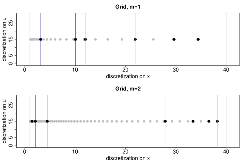
Figure 1: Chosen grid for modes 1 and 2. Black dots are centers of Voronoi cells that are constructed in order to respect boundary constraints. Grey dots are added to reduce the maximal cell diameter. Vertical lines indicate constraints related to boundaries: orange for $D$, blue for $\zeta_{0}$.

Once the grid is fixed, kernel $\bar{P}$ can be computed through Monte Carlo approximations for each point $\omega^{i}$ of the grid and each decision $d=(\ell,r)$.

5.2.2 Construction of the second grid

As the process (and its filter) are not simulatable (at least not simulatable according to all sets of possible strategies in sufficiently short time), the second discretization grid cannot be constructed based on simulation strategies such as quantization. Here the space to discretize is $\bar{\mathbb{X}}^{\prime}$ which dimension is that of $\mathcal{P}(\Omega)\times\mathbb{O}$, that is $({n_{\Omega}}-1)+3$. Choosing a relevant grid, in this context, is not trivial. In particular, even if we are given a fixed grid, the kernels $\hat{R}$ cannot be estimated directly by Monte Carlo simulation and projection as we are not able to simulate a $(\theta,y,z,w)$ from a given point $\rho^{i}$. We therefore need to compute directly the $\hat{R}(\rho^{j}|\rho^{i},d)$ using the approximate filters and kernels $\bar{{\Psi}}$ and $\bar{P}$ from the previous discretization.

The first thing we can notice is that it is not necessary to discretize the last dimension of $\mathbb{O}$, corresponding to $W$ the time spent since the beginning as it is already discrete along trajectories, $W$ being a multiple of $\delta$. The second dimension of $\mathbb{O}$ corresponds to $Z$, the observation of the death of the patient, which is also already discrete. Finally, the first dimension of $\mathbb{O}$ does not need to be discretized either. Indeed, the transition kernels $\hat{R}$ do not depend on $y$. The integral on $y^{\prime}$ over $I$ can be estimated by Monte Carlo approximation on the noise variable $\varepsilon$ once and for all. Given these remarks we need to discretize the $({n_{\Omega}}-1)$ simplex of $\mathbb{R}^{n_{\Omega}}$. After extensive stimulation studies, we recommend starting from a minimal fixed grid that we enrich through iterative simulations. More precisely, our strategy is the following.

Compute an initial grid with ${n_{\Omega}}$ points: for each element $\omega^{i}$ of $\Omega$ we define a probability vector that charges $\omega^{i}$ with probability $0.95$, the rest of the mass being distributed randomly through a Dirichlet distribution (with $\alpha=1$) on all other elements of $\Omega$; estimate $\hat{R}$ by Monte Carlo simulations.

Compute optimal strategies according to section 4.4 on this initial grid.

While some stopping criteria is not reached,

• simulate trajectories with the optimal strategy from the current grid;

• for each trajectory, at each time-point, compute the distances between the estimated filter and its projection on the current grid, and add all estimated filters which distances are larger than a threshold $s$ to form the next grid;

• estimate $\hat{R}$ by Monte Carlo simulations, and run dynamic programming to compute optimal strategies.

Different stopping criteria can be used, among which: a minimal number of points in the grid, a maximal proportion of distances larger than $s$, or a minimal decrease of value function between successive grids. See section E.3 for some further discussion and numerical experimentations. Note that these new grids allow to significantly reduce the distances between estimated filters and their projections. However, these improved grids are cost-dependent as dynamic programming optimizes the strategies based on the cost values. This implies that new grids have to be computed when costs change.

5.3 Strategies in competition and performance criteria

To evaluate the performance of our approach (OS in the comparison tables) we will compare our work with several other strategies.

The (unachievable) gold standard strategy is the See All (SA) where decisions are taken while observing the process $X_{t_{n}}$ by choosing the optimal treatment for the current mode. In this SA strategy, we do not allow choice of the next visit date.

The filter strategy corresponds to choosing the optimal treatment for the estimated mode: at each new observation $y_{n}$ the approximate filter $\bar{\theta}_{n}$ is computed based on the first discretization. Then the most probable mode $\hat{m}_{n}$ is obtained as

$$\hat{m}_{n}=\arg\max_{m=0:3}\sum_{j|\omega^{j}_{1}=m}\bar{\theta}_{n}^{j}.$$

Note that to set up this strategy, only the first discretization is needed. As this discretization is the least computationally extensive, it might be worth designing larger grids $\Omega$ to obtain better mode estimates. However, this strategy does not take into account knowledge on the dynamics of the process, hence we expect it to have higher costs. It is not able to select the next decision date either.

The Standard strategy is classically used in the hospitals and is based on thresholds $s_{rel}$ for relapse, and $s_{rem}$ for remission. While the observations remain below $s_{rel}$, the patient does not receive treatment and visits are scheduled every 2 months. When $s_{rel}$ is reached, the practitioner gives treatment $b$ (corresponding to the most frequent relapse type $2$) and the next visit is scheduled in $15$ days. If at the next visit the observed marker level has decreased, treatment $b$ is maintained with visits every $15$ days until $s_{rem}$ is reached. Otherwise the practitioner changes treatment for treatment $a$ (with visits every $15$ days.) Once $s_{rem}$ is reached, treatment is stopped, visits are scheduled every two months and the strategy is repeated.

The fixed dates optimal strategies are the strategies based on our discretization and dynamic programming approach where the choice of the next visit date are not allowed. We will investigate the fixed dates every $15$ and $60$ days (FD-15 and FD-60 in the comparison tables).

Performance criteria will include the real cost of each strategy evaluated on the real process $X$ (averaged over $500$ simulations), the estimated cost evaluated using the estimated filter and cost functions $c^{\prime}$ and $C^{\prime}$, and their average number of visits (recall that this number may vary due to the possible choice of next visit date for our strategy, but also because patients may die before the horizon $H$ is reached). When comparing only our strategy with the Fixed dates, we also compare the value of $\hat{v}_{0}$ computed by dynamic programming.

5.4 Results

First, note that all tables presented in this section have been created using Sweave, and all bits of codes are available online at
https://github.com/acleynen/PDMP-control.
All results presented here are based on $500$ simulations. The exact specifications and further numerical investigations can be found in the section E.

We first compare the use of two different distances on $\Gamma$: the $L_{2}$ distance, and distance $L_{m}$, which brings closer filters with same amount of mass on each modes: $L_{m}(\theta_{1},\theta_{2})=L_{2}(\theta_{1},\theta_{2})+|m_{1}^{0}-m_{2}^{0}|+|m_{1}^{1}-m_{2}^{1}|+|m_{1}^{2}-m_{2}^{2}|$ where $m_{j}^{i}=\sum_{k|\omega^{k}\in E_{i}}\theta_{j}(\omega^{k})$. We compare these on the initial grid (of size $184$, same grid for both distances) and on two grids of size approximately $1000$ calibrated by simulation using each distance. Results are summarized in table 1.

Table 1: Impact of distance choice the cost. For each of the minimal and fully updated grids, and comparing the fixed dates to the choice of return dates strategies. The impact is measured in terms of value function, real (Monte Carlo) costs of strategies, and estimated costs through projections.

			$L_{2}$			$L_{m}$
	strategy	$\hat{v}_{0}$	real cost (sd)	est. cost (sd)	$\hat{v}_{0}$	real cost (sd)	est. cost (sd)
	OS	194.77	197.85 (7.62)	193.17 (2.99)	195.42	179.09 (7.14)	175.52 (2.16)
Grid	FD-15	380.07	213.22 (2.51)	215.99 (0.92)	387.86	209.26 (2.4)	211.29 (0.76)
$184$	FD-60	196.78	201.07 (7.99)	195.05 (3.2)	197.50	184.77 (7.72)	175.91 (2.27)
	OS	125.23	168.79 (4.45)	167.48 (1.74)	132.43	136.78 (3.95)	134.62 (0.74)
Grid	FD-15	254.58	235.08 (2.84)	240.21 (1.97)	253.28	214.21 (1.67)	215.73 (0.78)
$\sim 1000$	FD-60	180.64	173.12 (6.68)	171.69 (2.97)	163.57	142.86 (5.29)	141.62 (1.04)

When the grid is too sparse ($n_{\Gamma}=184$) changing the distance does not improve the results, as the projected filters seldom differ. Calibrating larger grids through simulations significantly improves the performance of our approach, in particular for the $L_{m}$ distance. The gain is significant from the first iteration, and reach convergence really quickly (grids of size $\sim 700$ points achieve similar performance as those presented here).

As the exponential flows at first increase very slowly with respect to the noise of the observations, the FD-60 strategy benefits from the decision delay, thus decreasing the number of wrong decisions. On the contrary, the marker-dependent cost penalizes high values of the marker, hence might prefer wrong decisions to prevent jumps. It favors small return dates $r$ when the marker increases (area under curve (AUC) approximated by histograms from above) and large values of $r$ when the marker decreases (AUC approximated by histograms from below), hence a real effect of choosing visit dates. As a consequence, the average length of trajectories are longer with the marker-dependent cost, rising from $57$ visits with the $L_{2}$ distance and time-dependent cost (resp $54$ with the $L_{m}$ distance) to $65$ (resp $63$). For comparison, the length of FD-15 strategies are $161$, and $41$ for FD-60 strategies.

The most significant gain comes from the use of the $L_{m}$ distance, which favors projected filters with same mass on each mode as the estimated one. As a consequence, $\hat{\theta}_{n+1}$ under the $L_{m}$ distance is expected to be closer to $\bar{\theta}_{n+1}$ than $\hat{\theta}_{n+1}$ under the $L_{2}$ distance, hence the decisions match the reality of the process better.

Comparing this strategy with the Sea All, Filter and Standard strategies shows the added value of taking into account the knowledge on the dynamics of the process: it performs significantly better. This is particularly true when using the $L_{m}$ distance (results shown in table 2).

Table 2: Strategy comparisons. Performance of each strategy measured in terms of value function, real (Monte Carlo) costs of strategies, and estimated costs through projections.

	Visits	real cost (sd)	est. cost (sd)
	Choice	136.23 (3.91)	134.74 (0.82)
OS	15 days	213.92 (1.66)	215.16 (0.75)
	60 days	145.37 (4.94)	140.58 (0.99)
	15 jours	209.96 (2.38)	210.2 (0.72)
Filter	60 jours	169.39 (6.76)	170.56 (2.15)
	15 days	161.51 (0.04)
See All	60 days	52.31 (0.82)
Standard		438.92 (20.42)

6 Conclusion

We have proposed a numerically feasible scheme to approximate the value function of an impulse control problem for a class of hidden PDMPs where control actions do influence the dynamic of the process. Approximations rely on discretization of the observed and unobserved state spaces, for which we propose strategies to explore the large-dimensional belief spaces that depend on the process characteristics while maintaining error bounds for this approximation explicitly depending on the parameters of the problem. Codes are made freely available on Github.

This provides a mathematical setting to study realistic processes for instance in a disease-control framework, which we illustrate on simulations. This is a promising start for the study of even more realistic disease-control frameworks.

Finally, the important open question concerns the optimality of our candidate strategy. It cannot be directly linked to our various op- erators, but we are hopeful that further work will enable us to prove theoretically that it is close to optimality.

Appendix A Skeleton kernels of the controlled continuous-time PDMP

The generic form of the transition kernels $P$ of the skeleton chains with time span $r$ is formally given below. As there are at most 2 jumps (at most one random jump and 1 boundary jump), the generic form of $P$ for all $x=(m,\zeta,u)\in E_{M}$, $d=(\ell,r)\in L\times\mathbb{T}$ and any bounded measurable function $h$ on $E_{M}$ is

$$Ph(x,d)$$

$$= \mathbb{E}[h(X_{r})|X_{0}=x,d=(\ell,r)]$$

$$= h(\boldsymbol{\Phi}^{\ell}(x,r))e^{-\boldsymbol{\Lambda}^{\ell}(x,r)}\mathbbm{1}_{\boldsymbol{t}^{*\ell}(x)>r}$$ (2)

$$+\!\!\int_{0}^{r}\!\!\!\int_{E_{M}}\!\!\!\!\!\!h(\boldsymbol{\Phi}^{\ell}(x^{\prime},r-s))\boldsymbol{\lambda}^{\ell}(\boldsymbol{\Phi}^{\ell}(x,s))e^{-\boldsymbol{\Lambda}^{\ell}(x,s)}\boldsymbol{Q}^{\ell}(dx^{\prime}|\boldsymbol{\Phi}^{\ell}(x,s))\mathbbm{1}_{\boldsymbol{t}^{*\ell}(x)>s}\mathbbm{1}_{\boldsymbol{t}^{*\ell}(x^{\prime})>r-s}ds$$ (3)

$$+\int_{E_{M}}h(\boldsymbol{\Phi}^{\ell}(x^{\prime},r-\boldsymbol{t}^{*\ell}(x)))e^{-\boldsymbol{\Lambda}^{\ell}(x,\boldsymbol{t}^{*\ell}(x))}e^{-\boldsymbol{\Lambda}^{\ell}(x^{\prime},r-\boldsymbol{t}^{*\ell}(x))}$$

$$\qquad\qquad\qquad\boldsymbol{Q}^{\ell}(dx^{\prime}|\boldsymbol{\Phi}^{\ell}(x,\boldsymbol{t}^{*\ell}(x)))\mathbbm{1}_{\boldsymbol{t}^{*\ell}(x)\leq r}\mathbbm{1}_{\boldsymbol{t}^{*\ell}(x^{\prime})>r-\boldsymbol{t}^{*\ell}(x)}$$ (4)

$$+\int_{0}^{r-\boldsymbol{t}^{*\ell}(x)}\int_{E_{M}^{2}}h(\boldsymbol{\Phi}^{\ell}(x^{\prime\prime},r-\boldsymbol{t}^{*\ell}(x)-s))e^{-\boldsymbol{\Lambda}^{\ell}(x,\boldsymbol{t}^{*\ell}(x))}\boldsymbol{\lambda}^{\ell}(\boldsymbol{\Phi}^{\ell}(x^{\prime},s))e^{-\boldsymbol{\Lambda}^{\ell}(x^{\prime},s)}$$

$$\qquad\qquad\qquad\boldsymbol{Q}^{\ell}(dx^{\prime}|\boldsymbol{\Phi}^{\ell}(x,\boldsymbol{t}^{*\ell}(x)))\boldsymbol{Q}^{\ell}(dx^{\prime\prime}|\boldsymbol{\Phi}^{\ell}(x^{\prime},s))$$

$$\qquad\qquad\qquad\mathbbm{1}_{\boldsymbol{t}^{*\ell}(x)\leq r}\mathbbm{1}_{\boldsymbol{t}^{*\ell}(x^{\prime})>r-\boldsymbol{t}^{*\ell}(x)-s}\mathbbm{1}_{\boldsymbol{t}^{*\ell}(x^{\prime\prime})>r-\boldsymbol{t}^{*\ell}(x)-s}ds$$ (5)

$$+\int_{0}^{r}\int_{E_{M}^{2}}h(\boldsymbol{\Phi}^{\ell}(x^{\prime\prime},r-\boldsymbol{t}^{*\ell}(x^{\prime})-s))\boldsymbol{\lambda}^{\ell}(\boldsymbol{\Phi}^{\ell}(x,s))e^{-\boldsymbol{\Lambda}^{\ell}(x,s)}$$

$$\qquad\qquad\qquad\boldsymbol{Q}^{\ell}(dx^{\prime}|\boldsymbol{\Phi}^{\ell}(x,s))\boldsymbol{Q}^{\ell}(dx^{\prime\prime}|\boldsymbol{\Phi}^{\ell}(x^{\prime},\boldsymbol{t}^{*\ell}(x^{\prime})))\mathbbm{1}_{\boldsymbol{t}^{*\ell}(x)>s}\mathbbm{1}_{\boldsymbol{t}^{*\ell}(x^{\prime})\leq r-s}ds,$$ (6)

where $\boldsymbol{\Phi}^{\ell}(x,t)=(m,\Phi_{m}^{\ell}(\mathtt{x},t))$, $\boldsymbol{\lambda}^{\ell}(x)=\lambda_{m}^{\ell}(\mathtt{x})$, $\boldsymbol{\Lambda}^{\ell}(x,t)=\Lambda_{m}^{\ell}(\mathtt{x},t)$, $\boldsymbol{t}^{*\ell}(x)=\inf\{t>0:\Phi_{m}^{\ell}(\mathtt{x},t)\in\partial E_{m}^{\ell}\}$, and $\boldsymbol{Q}^{\ell}(\cdot|x)=Q_{m}^{\ell}(\cdot|x)$ is detailed in table 3.

Table 3: Markov kernel of the controlled continuous time PDMP: values of $Q_{m}^{\ell}(m^{\prime}|\zeta,u)$. Mode $m=3$ is omitted as no jump is allowed in this mode.

$\ell=\emptyset$	$m^{\prime}=0$	$m^{\prime}=1$	$m^{\prime}=2$	$m^{\prime}=3$
$m=0$	$0$	$Q_{m}^{\ell}(m^{\prime}|\zeta,u)\in(0,1)$	$1-Q_{m}^{\ell}(1|\zeta,u,w)$	$0$
$m=1,2$	$0$	$0$	$0$	$\mathbbm{1}_{\zeta=D}$
$\ell=a$	$m^{\prime}=0$	$m^{\prime}=1$	$m^{\prime}=2$	$m^{\prime}=3$
$m=0$	$0$	$0$	$1$	$0$
$m=1$	$\mathbbm{1}_{\zeta=\zeta_{0}}$	$0$	$\mathbbm{1}_{\zeta\neq\zeta_{0}}$	$0$
$m=2$	$0$	$0$	$0$	$\mathbbm{1}_{\zeta=D}$
$\ell=b$	$m^{\prime}=0$	$m^{\prime}=1$	$m^{\prime}=2$	$m^{\prime}=3$
$m=0$	$0$	$1$	$0$	$0$
$m=1$	$0$	$0$	$0$	$\mathbbm{1}_{\zeta=D}$
$m=2$	$\mathbbm{1}_{\zeta=\zeta_{0}}$	$\mathbbm{1}_{\zeta\neq\zeta_{0}}$	$0$	$0$

Each line corresponds to a specific behavior.

• Line (2) corresponds to the events where no jump has occurred and the process just followed the deterministic flow.

• Lines (3) and (4) correspond to the events where a single jump occurs. This jump can be

  • either a random jump (Line (3))

  • or a boundary jump at either $\zeta_{0}$ or $D$ (Line (4)).

• Lines (5) and (6) correspond to the events where two jumps occur, which can happen in either of two ways:

  • a boundary jump at $\zeta_{0}$ followed by a random jump (Line (5)).

  • a random jump followed by a boundary jump at $D$ (Line (6)).

Depending on the values of $x$ and $r$, some terms may have zero value in the formula above.

Appendix B Stability of kernels $R^{\prime}$ and $\bar{R}^{\prime}$

B.1 Kernel $R^{\prime}$ maps $\mathbb{X}^{\prime}$ onto itself

Set $\xi\in\mathbb{X}^{\prime}$ and $d\in\mathbb{K}^{\prime}(\xi)$, and denote $\Xi$ a random variable with distribution $R^{\prime}(\cdot|\xi,d)$. If $d=\check{d}$ then $\Xi=\Delta\in\mathbb{X}^{\prime}$. Otherwise, by definition one has $\xi=(\theta,y,z,w)$ such that $\theta(E_{0:2})=1$ or $\theta(E_{3})=1$; if $\theta(E_{0:2})=1$, then $\theta(E_{0})\geq\Big{(}\frac{\underline{f}}{\overline{f}}\Big{)}^{\frac{w}{\delta}\vee 1}e^{-w\|\lambda\|}$; if $\theta(E_{3})=1$, then $y=0$ and $z=1$; and $d=(\ell,r)\in\mathbb{K}^{\prime}(\xi)$. If $\theta(E_{3})=1$, then $y=0$ and $z=1$ so that $d=\check{d}$ and this case has already been treated. If $\theta(E_{0:2})=1$, then either $\Xi=(\Theta,Y,Z,W)$ with $Y=0$, $Z=1$ and thus $\Theta(E_{3})=1$, or $\Xi=(\Theta,Y,Z,W)$ with $Z=0$ and conditionally to $Y$,

$$\Theta=\Psi(\theta,Y,0,w+r,d),$$

and the definition of $\Psi$ directly yields $\Theta(E_{0:2})=1$. To obtain the lower bound on $\Theta(E_{0})$, note that

$$\Theta(E_{0}) =\frac{\int_{E_{0:2}}\int_{E_{0:2}}f(Y-F(x^{\prime}))\mathbbm{1}_{E_{0}}(x^{\prime})P(dx^{\prime}|x,d)\theta(dx)}{\int_{E_{0:2}}\int_{E_{0:2}}f(Y-F(x^{\prime}))P(dx^{\prime}|x,d)\theta(dx)}.$$

By definition of kernel $P$, if $x\in E_{0}$ and $d=(\ell,r)$, one has

$$P(E_{0}|x,d)=e^{-\boldsymbol{\Lambda}^{\ell}(x,r)}\geq e^{-r\|\lambda\|},$$

thanks to Assumption 3.6. Assumption 3.8 then yields

$$\Theta(E_{0}) \geq\frac{\underline{f}e^{-r\|\lambda\|}\theta(E_{0})}{\overline{f}}\geq\Big{(}\frac{\underline{f}}{\overline{f}}\Big{)}^{\frac{w+r}{\delta}\vee 1}e^{-(w+r)\|\lambda\|},$$

as $\frac{\underline{f}}{\overline{f}}\leq 1$ and $r\geq\delta$.

B.2 Kernel $\bar{R}^{\prime}$ maps $\bar{\mathbb{X}}^{\prime}$ onto itself

Set $\xi\in\bar{\mathbb{X}}^{\prime}$ and $d\in\mathbb{K}^{\prime}(\xi)$, and denote $\Xi$ a random variable with distribution $\bar{R}^{\prime}(\cdot|\xi,d)$. If $d=\check{d}$ then $\Xi=\Delta\in\bar{\mathbb{X}}^{\prime}$. Otherwise, by definition one has $\xi=(\theta,y,z,w)$ such that $\theta(\Omega_{0:2})=1$ or $\theta(\Omega_{3})=1$; if $\theta(\Omega_{0:2})=1$, then $\theta(\Omega_{0})\geq\Big{(}\frac{\underline{f}}{\overline{f}}\Big{)}^{\frac{w}{\delta}\vee 1}e^{-w\|\lambda\|}$; if $\theta(\Omega_{3})=1$, then $y=0$ and $z=1$; and $d=(\ell,r)\in\mathbb{K}^{\prime}(\xi)$. If $\theta(\Omega_{3})=1$, as above, $d=\check{d}$ and this case has already been treated. If $\theta(\Omega_{0:2})=1$, then either $\Xi=(\Theta,Y,Z,W)$ with $Y=0$, $Z=0$ and $\Xi(\Omega_{3})=1$ or $\Xi=(\Theta,Y,Z,W)$ with $Z=0$, and conditionally to $Y$,

$$\Theta={\bar{\Psi}}(\theta,Y,0,w+r,d),$$

and the definition of ${\bar{\Psi}}$ directly yields $\Theta(\Omega_{0:2})=1$. To obtain the lower bound on $\Theta(\Omega_{0})$, for all $\omega^{i}\in\Omega_{0:2}$, one has

$$\Theta(E_{0})(\omega^{j}) =\frac{\sum_{\omega^{i}\in\Omega_{0:2}}f(Y-F(\omega^{j}))\mathbbm{1}_{\Omega_{0:2}}(\omega^{j})\bar{P}(\omega^{j}|\omega^{i},d){\bar{\theta}}(\omega^{i})}{\sum_{\omega^{i}\in\Omega_{0:2}}\sum_{\omega^{k}\in\Omega_{0:2}}f(Y-F(\omega^{k}))\bar{P}(\omega^{k}|\omega^{i},d){\bar{\theta}}(\omega^{i})}$$

By definition of kernel $P$, if $\omega^{i}\in E_{0}$ and $d=(\ell,r)$, one has $\bar{P}(\Omega_{0}|\omega^{i},d)=P(E_{0}|x,d)\geq e^{-r\|\lambda\|}$ thanks to Assumptions 3.6 and 4.1 as the Voronoi cells form a partition of $E_{M}$ that preserves the mode.Assumption 3.8 then yields

$$\Theta(E_{0})\geq\frac{\underline{f}e^{-r\|\lambda\|}\theta(E_{0})}{\overline{f}}\geq\Big{(}\frac{\underline{f}}{\overline{f}}\Big{)}^{\frac{w+r}{\delta}\vee 1}e^{-(w+r)\|\lambda\|}.$$

Appendix C Error bounds for the first discretization

We introduce some function spaces compatible with the partition defined in section 4.1. Let $BL(E)$ be the set of Borel functions from $\mathbb{X}$ onto $\mathbb{R}$ for which there exist finite constants $\|\varphi\|_{E}$ and $[\varphi]_{E}$ such that for all $(x,\gamma)$ and $(x^{\prime},\gamma)$ in $\mathbb{X}-\{\Delta\}$, one has

• $|\varphi(\Delta)|\leq\|\varphi\|_{E}$, $|\varphi(x,\gamma)|\leq\|\varphi\|_{E},$

• $|\varphi(x,\gamma)-\varphi(x^{\prime},\gamma)|\leq[\varphi]_{E}\ \|x-x^{\prime}\|$, if $x$ and $x^{\prime}$ belong to the same subset $F_{j}$,

• $\varphi$ is constant on $(E_{3}\times\mathbb{O})\cap\mathbb{X}$.

Denote also the unit ball of $BL(E)$ by

$$BL_{1}(E) = \big{\{}\varphi\in BL(E):\|\varphi\|_{E}+[\varphi]_{E}\leq 1\big{\}}.$$

For $\theta$ and ${\bar{\theta}}$ two probability measures in $\mathcal{P}(E_{M})$, define the distance $d_{E}(\theta,{\bar{\theta}})$ by

$$d_{E}(\theta,{\bar{\theta}})=\sup_{g\in BL_{1}(E)}\sup_{\gamma\in\mathbb{O}}\left|\int\!\!\!g(x,\gamma){\mathbbm{1}_{\mathbb{X}}(x,\gamma)}\theta(dx)-\!\!\int\!\!\!g(x,\gamma){\mathbbm{1}_{\mathbb{X}}(x,\gamma)}{\bar{\theta}}(dx)\right|.$$

Let $BLP(E)$ be the set of Borel functions from $\mathbb{X}^{\prime}$ onto $\mathbb{R}$ for which there exist finite constants $\|\varphi\|_{E,\mathcal{P}}$ and $[\varphi]_{E,\mathcal{P}}$ such that for all $(\theta,\gamma)$ and $({\bar{\theta}},\gamma)$ in $\mathbb{X}^{\prime}$ such that $\theta(E_{0:2})={\bar{\theta}}(E_{0:2})=1$ or $\theta(E_{3})={\bar{\theta}}(E_{3})=1$ one has

• $|\varphi(\Delta)|\leq\|\varphi\|_{E,\mathcal{P}}$,

• $|\varphi(\theta,\gamma)|\leq\|\varphi\|_{E,\mathcal{P}}$,

• $|\varphi(\theta,\gamma)-\varphi({\bar{\theta}},\gamma)|\leq[\varphi]_{E,\mathcal{P}}d_{E}(\theta,{\bar{\theta}})$,

• $\varphi$ is constant on the set $\{(\theta,\gamma)\in\mathbb{X}^{\prime}-\{\Delta\}\ ;\ \theta(E_{3})=1\}$.

Denote also the unit ball of $BLP(E)$ by

$$BLP_{1}(E) = \big{\{}\varphi\in BLP(E):\|\varphi\|_{E,\mathcal{P}}+[\varphi]_{E,\mathcal{P}}\leq 1\big{\}}.$$

Finally, for any function $h\in BL(E)$, $\xi=(x,\gamma)\in\mathbb{X}-\{\Delta\}$ and $d\in\mathbb{K}(\xi)$, denote with a slight abuse of notation

$$Ph(\xi,d)=\int_{E_{M}}h(x^{\prime},\gamma^{\prime})P(dx^{\prime}|x,d),$$

with $\gamma^{\prime}=(y\mathbbm{1}_{(x^{\prime}_{1}\leq 3)},\mathbbm{1}_{(x^{\prime}_{1}=3)},w+r)$ if $\gamma=(y,z,w)$ and $d=(\ell,r)$.

The proof of Theorem 4.2 is split into a number of intermediate propositions and lemmas stated in the sequel. Most of the proofs rely on similar ideas, namely adequate splitting of expressions into simpler terms, and exploitation of Lipschitz regularity.

C.1 Regularity of operator $P$

The first key step is to obtain the local regularity of $P$ on our partition.

Proposition C.1

Under Assumption 3.6 and 3.7, there exists a positive constant $C_{P}$ such that for all $h\in BL_{1}(E)$, for all $x^{1}$ and $x^{2}$ belonging to the same subset $F_{j}$ of $E_{M}$, for all $(y,z,w)\in\mathbb{O}$ and $d\in\mathbb{K}(z,w)-\{\check{d}\}$, one has

$$\big{|}Ph(x^{1},y,z,w,d)-Ph(x^{2},y,z,w,d)\big{|} \leq C_{P}\|x^{1}-x^{2}\|,$$

in addition, $P$ maps $BL(E)$ onto itself and for $g\in BL(E)$, one has $\|Pg\|_{E}\leq\|g\|_{E}$ and $[Pg]_{E}\leq C_{P}(\|g\|_{E}+[g]_{E})$.

Proof First note that if $x^{1}$ and $x^{2}$ have different modes, the result holds true as the right-hand side equals infinity. In addition, note that $P$ maps $E_{3}$ onto itself, as no jump is possible in mode $3$. Therefore, if $x^{1}$ and $x^{2}$ belong to $E_{3}$, then $Ph(x^{1},y,z,w,d)=Ph(x^{2},y,z,w,d)$ as $h$ is constant on $E_{3}\times\mathbb{O}$. Hence, $Ph$ is also constant on $(E_{3}\times\mathbb{O})\cap\mathbb{X}$.

Second, note that if $z=1$, then $\mathbb{K}(z,w)=\{\check{d}\}$ and there is nothing to prove.

Suppose now that $x^{1}$ and $x^{2}$ share same mode $x^{1}_{1}=x^{2}_{1}=m$. Select $(y,z,w)\in\mathbb{O}$, $d=(\ell,r)\in\mathbb{K}(z,w)$ and a function $h\in BL_{1}(E)$ and denote $\gamma=(y,z,w)$ and $\gamma^{\prime}=(y,0,w+r)\mathbbm{1}_{x^{\prime}_{1}\neq 3}+(0,1,w+r)\mathbbm{1}_{x^{\prime}_{1}=3}$. As operator $P$ involves indicator functions, we split the computation of the difference $\big{|}Ph(x^{1},y,z,w,d)-Ph(x^{2},y,z,w,d)\big{|}$ into 3 cases depending on the values of $\boldsymbol{t}^{*\ell}(x^{1})$ and $\boldsymbol{t}^{*\ell}(\ell,x^{2})$ compared to $r$.

$\bullet$ First case: $\boldsymbol{t}^{*\ell}(x^{1})>r$ and $\boldsymbol{t}^{*\ell}(x^{2})>r$. In this case, the explicit formula in appendix A becomes

$$\big{|}Ph(x^{1},y,z,w,d)-Ph(x^{2},y,z,w,d)\big{|}$$

$$\leq\left|h(\boldsymbol{\Phi}^{\ell}(x^{1},r),\gamma^{\prime})e^{-\boldsymbol{\Lambda}^{\ell}(x^{1},r)}-h(\boldsymbol{\Phi}^{\ell}(x^{2},r),\gamma^{\prime})e^{-\boldsymbol{\Lambda}^{\ell}(x^{2},r)}\right|$$

$$+\left|\int_{0}^{r}\int_{E_{M}}\!\!\!h(\boldsymbol{\Phi}^{\ell}(x^{\prime},r-s),\gamma^{\prime})\boldsymbol{\lambda}^{\ell}(\boldsymbol{\Phi}^{\ell}(x^{1},s))e^{-\boldsymbol{\Lambda}^{\ell}(x^{1},s)}\boldsymbol{Q}^{\ell}(dx^{\prime}|\boldsymbol{\Phi}^{\ell}(x^{1},s))\mathbbm{1}_{\boldsymbol{t}^{*\ell}(x^{\prime})>r-s}ds\right.$$

$$-\left.\int_{0}^{r}\int_{E_{M}}\!\!\!h(\boldsymbol{\Phi}^{\ell}(x^{\prime},r-s),\gamma^{\prime})\boldsymbol{\lambda}^{\ell}(\boldsymbol{\Phi}^{\ell}(x^{2},s))e^{-\boldsymbol{\Lambda}^{\ell}(x^{2},s)}\boldsymbol{Q}^{\ell}(dx^{\prime}|\boldsymbol{\Phi}^{\ell}(x^{2},s))\mathbbm{1}_{\boldsymbol{t}^{*\ell}(x^{\prime})>r-s}ds\right|$$

$$+\left|\int_{0}^{r}\int_{E_{M}^{2}}\!\!\!h(\boldsymbol{\Phi}^{\ell}(x^{\prime\prime},r-\boldsymbol{t}^{*\ell}(x^{\prime})-s),\gamma^{\prime})\boldsymbol{\lambda}^{\ell}(\boldsymbol{\Phi}^{\ell}(x^{1},s))e^{-\boldsymbol{\Lambda}^{\ell}(x^{1},s)}\right.$$

$$\qquad\qquad\boldsymbol{Q}^{\ell}(dx^{\prime}|\boldsymbol{\Phi}^{\ell}(x^{1},s))\boldsymbol{Q}^{\ell}(dx^{\prime\prime}|\boldsymbol{\Phi}^{\ell}(x^{\prime},\boldsymbol{t}^{*\ell}(x^{\prime})))\mathbbm{1}_{\boldsymbol{t}^{*\ell}(x^{\prime})\leq r-s}ds$$

$$-\int_{0}^{r}\int_{E_{M}^{2}}h(\boldsymbol{\Phi}^{\ell}(x^{\prime\prime},r-\boldsymbol{t}^{*\ell}(x^{\prime})-s),\gamma^{\prime})\boldsymbol{\lambda}^{\ell}(\boldsymbol{\Phi}^{\ell}(x^{2},s))e^{-\boldsymbol{\Lambda}^{\ell}(x^{2},s)}$$

$$\qquad\qquad\left.\boldsymbol{Q}^{\ell}(dx^{\prime}|\boldsymbol{\Phi}^{\ell}(x^{2},s))\boldsymbol{Q}^{\ell}(dx^{\prime\prime}|\boldsymbol{\Phi}^{\ell}(x^{\prime},\boldsymbol{t}^{*\ell}(x^{\prime})))\mathbbm{1}_{\boldsymbol{t}^{*\ell}(x^{\prime})\leq r-s}ds\right|$$

$$=A_{1}+B_{1}+C_{1}.$$

We split the expression into a sum of 3 terms that we study separately.

$\star$Term $A_{1}$: This term corresponds to no jump occurring. As $h$ is in $BL_{1}(E)$ on obtains from Assumptions 3.6 and 3.7 that

$$A_{1} \leq\left|h(\boldsymbol{\Phi}^{\ell}(x^{1},r),\gamma^{\prime})-h(\boldsymbol{\Phi}^{\ell}(x^{2},r),\gamma^{\prime})\right||e^{-\boldsymbol{\Lambda}^{\ell}(x^{1},r)}|$$

$$\quad+\left|h(\boldsymbol{\Phi}^{\ell}(x^{2},r),\gamma^{\prime})\right||e^{-\boldsymbol{\Lambda}^{\ell}(x^{1},r)}-e^{-\boldsymbol{\Lambda}^{\ell}(x^{2},r)}|$$

$$\leq[h][\Phi]\|x^{1}-x^{2}\|+\|h\|r[\lambda]{[\Phi]}\|x^{1}-x^{2}\|$$

$$\leq{[\Phi](1+\bar{\delta}[\lambda])}\|x^{1}-x^{2}\|,$$

where $\bar{\delta}=\max\mathbb{T}$.

$\star$Term $B_{1}$: This term corresponds to one random jump, which can only lead to modes $1$ or $2$. We therefore split this term in $2$ parts that can be controlled identically:

$$B_{1}$$

$$\leq\sum_{i=1}^{2}\!\left|\int_{0}^{r}\!\!\!\!\int_{E_{i}}\!\!\!\!h(\boldsymbol{\Phi}^{\ell}(x^{\prime},r-s),\gamma^{\prime})\boldsymbol{\lambda}^{\ell}(\boldsymbol{\Phi}^{\ell}(x^{1},s))e^{-\boldsymbol{\Lambda}^{\ell}(x^{1},s)}\boldsymbol{Q}^{\ell}(dx^{\prime}|\boldsymbol{\Phi}^{\ell}(x^{1},s))\mathbbm{1}_{\boldsymbol{t}^{*\ell}(x^{\prime})>r-s}ds\right.$$

$$-\left.\int_{0}^{r}\!\!\!\int_{E_{i}}\!\!\!\!h(\boldsymbol{\Phi}^{\ell}(x^{\prime},r-s),\gamma^{\prime})\boldsymbol{\lambda}^{\ell}(\boldsymbol{\Phi}^{\ell}(x^{2},s))e^{-\boldsymbol{\Lambda}^{\ell}(x^{2},s)}\boldsymbol{Q}^{\ell}(dx^{\prime}|\boldsymbol{\Phi}^{\ell}(x^{2},s))\mathbbm{1}_{\boldsymbol{t}^{*\ell}(x^{\prime})>r-s}ds\right|$$

$$\leq\sum_{i=1}^{2}\left|\int_{0}^{r}\!\!\!\!h(i,\Phi_{i}^{\ell}(m,\Phi_{m}^{\ell}(x^{1},s),r-s),\gamma^{\prime})\boldsymbol{\lambda}^{\ell}(\boldsymbol{\Phi}^{\ell}(x^{1},s))e^{-\boldsymbol{\Lambda}^{\ell}(x^{1},s)}\mathbbm{1}_{t_{i}^{*\ell}(\Phi_{m}^{\ell}(x^{1}_{2},s))>r-s}\ ds\right.$$

$$\ -\left.\int_{0}^{r}\!\!\!\!h(i,\Phi_{i}^{\ell}(m,\Phi_{m}^{\ell}(m,x^{2},s),r-s),\gamma^{\prime})\boldsymbol{\lambda}^{\ell}(\boldsymbol{\Phi}^{\ell}(x^{2},s))e^{-\boldsymbol{\Lambda}^{\ell}(x^{2},s)}\mathbbm{1}_{t_{i}^{*\ell}(\Phi_{m}^{\ell}(x^{2}_{2},s))>r-s}\ ds\right|$$

$$=B_{11}+B_{12}$$

Moreover, this jump can only happen if coming initially from mode $m=0$, in which case $\Phi_{m}^{\ell}(x^{j},s)$ is constant, or from mode $1$ with control $b$ or mode $2$ with control $a$, in which case $\Phi_{m}^{\ell}(x^{j},s)$ is non-increasing, according to Assumption 3.3. In all cases, for the mode $i$ after the jump, $t_{i}^{*\ell}(x^{\prime})$ is non-increasing. To deal with the indicator functions in terms $B_{11}$ and $B_{12}$, we now consider 3 different subcases:
$\blacktriangle$ first sub-case: $t_{i}^{*\ell}(x^{1}_{2})>r$ and $t_{i}^{*\ell}(x^{2}_{2})>r$ (hence for all $0\leq s\leq r$, $t_{i}^{*\ell}(\Phi_{m}^{\ell}(x^{j}_{2},s))>r-s$). One has

$$B_{1i}$$

$$\leq\int_{0}^{r}\left|h(i,\Phi_{i}^{\ell}(m,\Phi_{m}^{\ell}(x^{1},s),r-s),\gamma^{\prime})-h(i,\Phi_{i}^{\ell}(m,\Phi_{m}^{\ell}(x^{2},s),r-s),\gamma^{\prime})\right|$$

$$\qquad\qquad\qquad\boldsymbol{\lambda}^{\ell}(\boldsymbol{\Phi}^{\ell}(x^{2},s))e^{-\boldsymbol{\Lambda}^{\ell}(x^{2},s)}\ ds$$

$$+\int_{0}^{r}\left|h(i,\Phi_{i}^{\ell}(m,\Phi_{m}^{\ell}(x^{1},s),r-s),\gamma^{\prime})\right|\left|\boldsymbol{\lambda}^{\ell}(\boldsymbol{\Phi}^{\ell}(x^{1},s))-\boldsymbol{\lambda}^{\ell}(\boldsymbol{\Phi}^{\ell}(x^{2},s))\right|e^{-\boldsymbol{\Lambda}^{\ell}(x^{2},s)}\ ds$$

$$+\int_{0}^{r}\left|h(i,\Phi_{i}^{\ell}(m,\Phi_{m}^{\ell}(x^{1},s),r-s),\gamma^{\prime})\boldsymbol{\lambda}^{\ell}(\boldsymbol{\Phi}^{\ell}(x^{1},s))\right|\left|e^{-\boldsymbol{\Lambda}^{\ell}(x^{2},s)}-e^{-\boldsymbol{\Lambda}^{\ell}(x^{2},s)}\right|\ ds$$

$$\leq[h][\Phi]^{2}\|x^{1}-x^{2}\|+r\|h\|[\lambda][\Phi]\|x^{1}-x^{2}\|+\|h\|\|\lambda\|r^{2}[\lambda]{[\Phi]}\|x^{1}-x^{2}\|$$

$$\leq\big{(}[\Phi]^{2}+\bar{\delta}[\lambda][\Phi]+\|\lambda\|\bar{\delta}^{2}[\lambda][\Phi]\big{)}\|x^{1}-x^{2}\|.$$

$\blacktriangle$ second sub-case: $t_{i}^{*\ell}(x^{1}_{2})<r$ and $t_{i}^{*\ell}(x^{2}_{2})<r$. Hence there exists $0<s_{i}^{1}<r$ and $0<s_{i}^{2}<r$ such that for all $s\leq s_{i}^{j}$, one has $t_{i}^{*\ell}(\Phi_{m}^{\ell}(x^{j}_{2},s))\leq r-s$, and for all $s\leq s_{i}^{j}$, one has $t_{i}^{*\ell}(\Phi_{m}^{\ell}(x^{j}_{2},s))>r-s$. Under Assumption 3.7, one also has $t_{i}^{*\ell}(\Phi_{m}^{\ell}(x^{j}_{2},s_{i}^{j}))=r-s_{i}^{j}$. Suppose, without loss of generality that $s_{i}^{1}\leq s_{i}^{2}$. Similar computations as in the previous sub-case lead to

$$B_{1i} \leq\left|\int_{s_{i}^{1}}^{s_{i}^{2}}h(i,\Phi_{i}^{\ell}(m,\Phi_{m}^{\ell}(x^{1},s),r-s),\gamma^{\prime})\boldsymbol{\lambda}^{\ell}(\boldsymbol{\Phi}^{\ell}(x^{1},s))e^{-\boldsymbol{\Lambda}^{\ell}(x^{1},s)}ds\right|$$

$$\qquad+\left|\int_{s_{i}^{2}}^{r}h(i,\Phi_{i}^{\ell}(m,\Phi_{m}^{\ell}(x^{1},s),r-s),\gamma^{\prime})\boldsymbol{\lambda}^{\ell}(\boldsymbol{\Phi}^{\ell}(x^{1},s))e^{-\boldsymbol{\Lambda}^{\ell}(x^{1},s)}ds\right.$$

$$\qquad-\left.\int_{s_{i}^{2}}^{r}h(i,\Phi_{i}^{\ell}(m,\Phi_{m}^{\ell}(m,x^{2},s),r-s),\gamma^{\prime})\boldsymbol{\lambda}^{\ell}(\boldsymbol{\Phi}^{\ell}(x^{2},s))e^{-\boldsymbol{\Lambda}^{\ell}(x^{2},s)}ds\right|$$

$$B_{1i} \leq\big{(}[\Phi]^{2}+\bar{\delta}[\lambda][\Phi]+\|\lambda\|\bar{\delta}^{2}[\lambda]{[\Phi]}\big{)}\|x^{1}-x^{2}\|+|s_{i}^{1}-s_{i}^{2}|$$

$$\leq\big{(}[\Phi]^{2}+\bar{\delta}[\lambda][\Phi]+\|\lambda\|\bar{\delta}^{2}[\lambda]{[\Phi]}+[S]\big{)}\|x^{1}-x^{2}\|.$$

$\blacktriangle$ other sub-cases: If $t_{i}^{*\ell}(x^{1}_{2})$ and $t_{i}^{*\ell}(x^{2}_{2})$ are on different sides of $r$, then the difference $\big{|}Ph(x^{1},\gamma,d)-Ph(x^{2},\gamma,d)\big{|}$ cannot be made arbitrarily small as $\|x^{1}-x^{2}\|$ is small. However, this case is impossible as $x^{1}$ and $x^{2}$ are in the same subset $F_{j}$.

$\star$Term $C_{1}$: Recall that this term comes from a first random jump followed by a boundary jump. Under our assumptions, this is only possible if $(m,\ell)\in\{(1,a),(2,b)\}$, the first random jump yields to mode $i\in\{1,2\}\neq m$, thus $\Phi_{m}^{\ell}$ is non increasing by Assumption 3.3, and the boundary jump is at $D$. In a similar manner as for $B_{1}$ we split the term as

$$C_{1} \leq\sum_{i=1}^{2}\left|\int_{0}^{r}h(3,D,r-t_{i}^{*\ell}(\Phi_{m}^{\ell}(x^{1}_{2},s))-s,\gamma^{\prime})\boldsymbol{\lambda}^{\ell}(\boldsymbol{\Phi}^{\ell}(x^{1},s))e^{-\boldsymbol{\Lambda}^{\ell}(x^{1},s)}\right.$$

$$\qquad\qquad\qquad\mathbbm{1}_{t_{i}^{*\ell}(\Phi_{m}^{\ell}(x^{1}_{2},s))\leq r-s}ds$$

$$\qquad-\int_{0}^{r}h(3,D,r-t_{i}^{*\ell}(\Phi_{m}^{\ell}(x^{2}_{2},s))-s,\gamma^{\prime\prime})\boldsymbol{\lambda}^{\ell}(\boldsymbol{\Phi}^{\ell}(x^{2},s))e^{-\boldsymbol{\Lambda}^{\ell}(x^{2},s)}$$

$$\qquad\qquad\qquad\left.\mathbbm{1}_{t_{i}^{*\ell}(\Phi_{m}^{\ell}(x^{2}_{2},s))\leq r-s}ds\right|$$

$$\leq C_{11}+C_{12}.$$

Note that only one term in the sum above is non-zero as $i\neq m$.
$\blacktriangle$ first sub-case: $t_{i}^{*\ell}(x^{1}_{2})>r$ and $t_{i}^{*\ell}(x^{2}_{2})>r$. Hence, as above, for all $0\leq s\leq r$, $t_{i}^{*\ell}(\Phi_{m}^{\ell}(x^{j}_{2},s))>r-s$ and $C_{1}$ has zero value.
$\blacktriangle$ second sub-case: $t_{i}^{*\ell}(x^{1}_{2})<r$ and $t_{i}^{*\ell}(x^{2}_{2})<r$. Then as above, there exists $0<s_{i}^{1}<r$ and $0<s_{i}^{2}<r$ such that for all $s\leq s_{i}^{j}$, one has $t_{i}^{*\ell}(\Phi_{m}^{\ell}(x^{j}_{2},s))\leq r-s$, and for all $s\leq s_{i}^{j}$, one has $t_{i}^{*\ell}(\Phi_{m}^{\ell}(x^{j}_{2},s))>r-s$. Under Assumption 3.7, one also has $t_{i}^{*\ell}(\Phi_{m}^{\ell}(x^{j}_{2},s_{i}^{j}))=r-s_{i}^{j}$. Suppose, without loss of generality that $s_{i}^{1}\leq s_{i}^{2}$. One has

$$C_{1i} \leq\int_{s_{i}^{1}}^{s_{i}^{2}}\left|\boldsymbol{\lambda}^{\ell}(\boldsymbol{\Phi}^{\ell}(x^{1},s))e^{-\boldsymbol{\Lambda}^{\ell}(x^{1},s)}\right|ds$$

$$\qquad+\int_{s_{i}^{2}}^{r}\big{|}h(3,D,r-t_{i}^{*\ell}(\Phi_{m}^{\ell}(x^{1}_{2},s))-s,\gamma)\boldsymbol{\lambda}^{\ell}(\boldsymbol{\Phi}^{\ell}(x^{1},s))e^{-\boldsymbol{\Lambda}^{\ell}(x^{1},s)}$$

$$\qquad-h(3,D,r-t_{i}^{*\ell}(\Phi_{m}^{\ell}(x^{2}_{2},s))-s,\gamma^{\prime})\boldsymbol{\lambda}^{\ell}(\boldsymbol{\Phi}^{\ell}(x^{2},s))e^{-\boldsymbol{\Lambda}^{\ell}(x^{2},s)}\big{|}ds$$

$$\leq([S]+[t^{*}][\Phi]+[\lambda][\Phi]\bar{\delta}+\|\lambda\|[\lambda][\Phi]\bar{\delta}^{2})\|x^{1}-x^{2}\|.$$

$\blacktriangle$ other sub-cases: We once again exclude other sub-cases by choosing $x^{1}$ and $x^{2}$ in the same subset $F_{j}$ of $E$.

$\bullet$ Second case: $\boldsymbol{t}^{*\ell}(x^{1})\leq r$ and $\boldsymbol{t}^{*\ell}(x^{2})\leq r$. This implies again that $m\in\{1,2\}$. We suppose, without loss of generality, that $\boldsymbol{t}^{*\ell}(x^{1})\leq\boldsymbol{t}^{*\ell}(x^{2})$. Then the difference $\left|Ph(x^{1},\gamma,d)-Ph(x^{2},\gamma,d)\right|$ can be split in 4 terms $A_{2}$, $B_{2}$, $C_{2}$ and $D_{2}$ corresponding to eqs. 3, 4, 5 and 6, depending on the jumps of the process.

$\star$ The first term corresponds to a single random jump. This is only possible if $i\in\{1,2\}\neq m$ and $\Phi_{m}^{\ell}$ is non increasing. One has

$$A_{2} \leq\sum_{i=1}^{2}\int_{0}^{\boldsymbol{t}^{*\ell}(x^{1})}\int_{E_{i}}\left|h(\boldsymbol{\Phi}^{\ell}(x^{\prime},r-s),\gamma^{\prime})\boldsymbol{\lambda}^{\ell}(\boldsymbol{\Phi}^{\ell}(x^{1},s))e^{-\boldsymbol{\Lambda}^{\ell}(x^{1},s)}\boldsymbol{Q}^{\ell}(dx^{\prime}|\boldsymbol{\Phi}^{\ell}(x^{1},s))\mathbbm{1}_{\boldsymbol{t}^{*\ell}(x^{\prime})>r-s}\right.$$

$$\qquad\left.-h(\boldsymbol{\Phi}^{\ell}(x^{\prime},r-s),\gamma^{\prime})\boldsymbol{\lambda}^{\ell}(\boldsymbol{\Phi}^{\ell}(x^{2},s))e^{-\boldsymbol{\Lambda}^{\ell}(x^{2},s)}\boldsymbol{Q}^{\ell}(dx^{\prime}|\boldsymbol{\Phi}^{\ell}(x^{2},s))\mathbbm{1}_{\boldsymbol{t}^{*\ell}(x^{\prime})>r-s}\right|ds$$

$$\quad+\sum_{i=1}^{2}\int_{\boldsymbol{t}^{*\ell}(x^{1})}^{\boldsymbol{t}^{*\ell}(x^{2})}\int_{E_{i}}\left|h(\boldsymbol{\Phi}^{\ell}(x^{\prime},r-s))\boldsymbol{\lambda}^{\ell}(\boldsymbol{\Phi}^{\ell}(x^{2},s))e^{-\boldsymbol{\Lambda}^{\ell}(x^{2},s)}\boldsymbol{Q}^{\ell}(dx^{\prime}|\boldsymbol{\Phi}^{\ell}(x^{2},s))\mathbbm{1}_{\boldsymbol{t}^{*\ell}(x^{\prime})>r-s}\right|ds.$$

Once again this term is studied by separating cases based on the position of $t_{i}^{*\ell}(x^{1})$ and $t_{i}^{*\ell}(x^{2})$ with respect to $r$. Then, similarly to term $B_{1}$ above, if $x^{1}$ and $x^{2}$ are in the same subset $F_{j}$ of $E$, we obtain

$$A_{2}\leq\big{(}[\Phi]^{2}+\bar{\delta}[\lambda][\Phi]+\|\lambda\|\bar{\delta}^{2}[\lambda]{[\Phi]}+[S]\big{)}\|x^{1}-x^{2}\|+[t^{*}]\|x^{1}-x^{2}\|.$$

$\star$ The second term corresponds to a single boundary jump at $\zeta_{0}$ or at $D$ :

$$B_{2} \leq\int_{E_{M}}\left|h(\boldsymbol{\Phi}^{\ell}(x^{\prime},r-\boldsymbol{t}^{*\ell}(x^{1})),\gamma^{\prime})e^{-\boldsymbol{\Lambda}^{\ell}(x^{1},\boldsymbol{t}^{*\ell}(x^{1}))}e^{-\boldsymbol{\Lambda}^{\ell}(x^{\prime},r-t^{*d}(x^{1}))}\right.$$

$$\qquad\qquad\qquad\boldsymbol{Q}^{\ell}(dx^{\prime}|\boldsymbol{\Phi}^{\ell}(x^{1},\boldsymbol{t}^{*\ell}(x^{1})))\mathbbm{1}_{\boldsymbol{t}^{*\ell}(x^{\prime})>r-\boldsymbol{t}^{*\ell}(x^{1})}$$

$$\qquad h(\boldsymbol{\Phi}^{\ell}(x^{\prime},r-\boldsymbol{t}^{*\ell}(x^{2})),\gamma^{\prime})e^{-\boldsymbol{\Lambda}^{\ell}(x^{2},\boldsymbol{t}^{*\ell}(x^{2}))}e^{-\boldsymbol{\Lambda}^{\ell}(x^{\prime},r-\boldsymbol{t}^{*\ell}(x^{2}))}$$

$$\qquad\qquad\qquad\left.\boldsymbol{Q}^{\ell}(dx^{\prime}|\boldsymbol{\Phi}^{\ell}(x^{2},\boldsymbol{t}^{*\ell}(x^{2})))\mathbbm{1}_{\boldsymbol{t}^{*\ell}(x^{\prime})>r-\boldsymbol{t}^{*\ell}(x^{2})}\right|.$$

Recall that since $x^{1}$ and $x^{2}$ have the same mode and the same decision $d$ is taken, thus this jump occurs at the same boundary for each term. Moreover, in either case we have $\boldsymbol{t}^{*\ell}(x^{\prime})=+\infty$. Therefore similar computations as in the first case lead to

$$B_{2}\leq([t^{*}]+\bar{\delta}[\lambda][\Phi]+\|\lambda\|[t^{*}])\|x^{1}-x^{2}\|.$$

$\star$ The third term corresponds to a boundary jump at $\zeta_{0}$ followed by a random jump to mode $i\in\{1,2\}\neq m$. It is only possible when the flow $\Phi_{m}^{\ell}$ is non increasing.

$$C_{2} \leq\sum_{i=1}^{2}\int_{0}^{r-\boldsymbol{t}^{*\ell}(x^{2})}\int_{E_{i}}\left|h(\boldsymbol{\Phi}^{\ell}(x^{\prime\prime},r-\boldsymbol{t}^{*\ell}(x^{1})-s),\gamma^{\prime\prime})e^{-\boldsymbol{\Lambda}^{\ell}(x^{1},\boldsymbol{t}^{*\ell}(x^{1^{\prime}}))}\boldsymbol{\lambda}^{\ell}(\boldsymbol{\Phi}^{\ell}(x^{1^{\prime}},s))\right.$$

$$\qquad\qquad e^{-\boldsymbol{\Lambda}^{\ell}(x^{1^{\prime}},s)}\boldsymbol{Q}^{\ell}(dx^{\prime\prime}|\boldsymbol{\Phi}^{\ell}(x^{1^{\prime}},s))\mathbbm{1}_{\boldsymbol{t}^{*\ell}(x^{1^{\prime}})>r-\boldsymbol{t}^{*\ell}(x^{1})-s}\mathbbm{1}_{\boldsymbol{t}^{*\ell}(x^{\prime\prime})>r-\boldsymbol{t}^{*\ell}(x^{1})-s}$$

$$-h(\boldsymbol{\Phi}^{\ell}(x^{\prime\prime},r-\boldsymbol{t}^{*\ell}(x^{2})-s),\gamma^{\prime\prime})e^{-\boldsymbol{\Lambda}^{\ell}(x^{2},\boldsymbol{t}^{*\ell}(x^{2}))}\boldsymbol{\lambda}^{\ell}(\boldsymbol{\Phi}^{\ell}(x^{2^{\prime}},s))$$

$$\qquad\qquad\left.e^{-\boldsymbol{\Lambda}^{\ell}(x^{2^{\prime}},s)}\boldsymbol{Q}^{\ell}(dx^{\prime\prime}|\boldsymbol{\Phi}^{\ell}(x^{2^{\prime}},s))\mathbbm{1}_{\boldsymbol{t}^{*\ell}(x^{2^{\prime}})>r-\boldsymbol{t}^{*\ell}(x^{2})-s}\mathbbm{1}_{\boldsymbol{t}^{*\ell}(x^{\prime\prime})>r-\boldsymbol{t}^{*\ell}(x^{2})-s}\right|ds$$

$$+\sum_{i=1}^{2}\int_{r-\boldsymbol{t}^{*\ell}(x^{2})}^{r-\boldsymbol{t}^{*\ell}(x^{1})}\int_{E_{i}}\left|h(\boldsymbol{\Phi}^{\ell}(x^{\prime\prime},r-\boldsymbol{t}^{*\ell}(x^{1})-s),\gamma^{\prime\prime})e^{-\boldsymbol{\Lambda}^{\ell}(x^{1},\boldsymbol{t}^{*\ell}(x^{1}))}\boldsymbol{\lambda}^{\ell}(\boldsymbol{\Phi}^{\ell}(x^{1^{\prime}},s))\right.$$

$$\qquad\qquad e^{-\boldsymbol{\Lambda}^{\ell}(x^{1^{\prime}},s)}\boldsymbol{Q}^{\ell}(dx^{\prime\prime}|\boldsymbol{\Phi}^{\ell}(x^{1^{\prime}},s))\mathbbm{1}_{\boldsymbol{t}^{*\ell}(x^{1^{\prime}})>r-\boldsymbol{t}^{*\ell}(x^{1})-s}\mathbbm{1}_{\boldsymbol{t}^{*\ell}(x^{\prime\prime})>r-\boldsymbol{t}^{*\ell}(x^{1})-s}\Big{|}ds$$

with $x^{1^{\prime}}=(0,\zeta_{0})$ and $x^{2^{\prime}}=(0,\zeta_{0},0)$ hence $\boldsymbol{t}^{*\ell}(x^{1^{\prime}})=\boldsymbol{t}^{*\ell}(x^{2^{\prime}})=+\infty$. Moreover, Assumption 3.4 prevents more than two jumps from happening between two decision dates, and therefore $\boldsymbol{t}^{*\ell}(x^{\prime\prime})>r-\boldsymbol{t}^{*\ell}(x^{j})$. Hence one has

$$C_{2} \leq\sum_{i=1}^{2}\int_{0}^{r-\boldsymbol{t}^{*\ell}(x^{2})}\int_{E_{i}}\left|h(\boldsymbol{\Phi}^{\ell}(x^{\prime\prime},r-\boldsymbol{t}^{*\ell}(x^{1})-s),\gamma^{\prime\prime})e^{-\boldsymbol{\Lambda}^{\ell}(x^{1},\boldsymbol{t}^{*\ell}(x^{1}))}\boldsymbol{\lambda}^{\ell}(\boldsymbol{\Phi}^{\ell}(x^{1^{\prime}},s))\right.$$

$$\qquad\qquad\qquad e^{-\boldsymbol{\Lambda}^{\ell}(x^{1^{\prime}},s)}\boldsymbol{Q}^{\ell}(dx^{\prime\prime}|\boldsymbol{\Phi}^{\ell}(x^{1^{\prime}},s))$$

$$\qquad-h(\boldsymbol{\Phi}^{\ell}(x^{\prime\prime},r-\boldsymbol{t}^{*\ell}(x^{2})-s),\gamma^{\prime})e^{-\boldsymbol{\Lambda}^{\ell}(x^{2},\boldsymbol{t}^{*\ell}(x^{2}))}\boldsymbol{\lambda}^{\ell}(\boldsymbol{\Phi}^{\ell}(x^{2^{\prime}},s))$$

$$\qquad\qquad\qquad\left.e^{-\boldsymbol{\Lambda}^{\ell}(x^{2^{\prime}},s)}\boldsymbol{Q}^{\ell}(dx^{\prime\prime}|\boldsymbol{\Phi}^{\ell}(x^{2^{\prime}},s))\right|ds$$

$$+\sum_{i=1}^{2}\int_{r-\boldsymbol{t}^{*\ell}(x^{2})}^{r-\boldsymbol{t}^{*\ell}(x^{1})}\int_{E_{i}}\left|h(\boldsymbol{\Phi}^{\ell}(x^{\prime\prime},r-\boldsymbol{t}^{*\ell}(x^{1})-s),\gamma^{\prime\prime})e^{-\boldsymbol{\Lambda}^{\ell}(x^{1},\boldsymbol{t}^{*\ell}(x^{1}))}\boldsymbol{\lambda}^{\ell}(\boldsymbol{\Phi}^{\ell}(x^{1^{\prime}},s))\right.$$

$$\qquad\qquad\qquad\left.e^{-\boldsymbol{\Lambda}^{\ell}(x^{1^{\prime}},s)}\boldsymbol{Q}^{\ell}(dx^{\prime\prime}|\boldsymbol{\Phi}^{\ell}(x^{1^{\prime}},s))\right|ds$$

$$\leq([t^{*}]+[\Phi][t^{*}]+\bar{\delta}[\lambda][\Phi]+[t^{*}]|\|\lambda\|+\bar{\delta}^{2}\|\lambda\|[\lambda][\Phi][t^{*}]+\bar{\delta}\|\lambda\|[\lambda][\Phi][t^{*}])\|x^{1}-x^{2}\|.$$

$\star$ The last term corresponds to a random jump to $i\in\{1,2\}\neq m$ followed by a boundary jump at $D$. It is treated similarly to term $C_{1}$. One has

$$D_{2} \leq\int_{0}^{\boldsymbol{t}^{*\ell}(x^{1})}\int_{E_{3}}\int_{E_{i}}\left|h(\boldsymbol{\Phi}^{\ell}(x^{\prime\prime},r-t^{*d}(x^{1})-s),\gamma^{\prime\prime})\boldsymbol{\lambda}^{\ell}(\boldsymbol{\Phi}^{\ell}(x^{1},s))e^{-\boldsymbol{\Lambda}^{\ell}(x^{1},s)}\right.$$

$$\qquad\qquad\qquad\boldsymbol{Q}^{\ell}(dx^{\prime}|\boldsymbol{\Phi}^{\ell}(x^{1},s))\boldsymbol{Q}^{\ell}(dx^{\prime\prime}|\boldsymbol{\Phi}^{\ell}(x^{\prime},\boldsymbol{t}^{*\ell}(x^{\prime})))\mathbbm{1}_{\boldsymbol{t}^{*\ell}(x^{\prime})\leq r-s}$$

$$\quad\qquad-h(\boldsymbol{\Phi}^{\ell}(x^{\prime\prime},r-t^{*d}(x^{2})-s),\gamma^{\prime\prime})\boldsymbol{\lambda}^{\ell}(\boldsymbol{\Phi}^{\ell}(x^{2},s))e^{-\boldsymbol{\Lambda}^{\ell}(x^{2},s)}$$

$$\qquad\qquad\qquad\left.\boldsymbol{Q}^{\ell}(dx^{\prime}|\boldsymbol{\Phi}^{\ell}(x^{2},s))\boldsymbol{Q}^{\ell}(dx^{\prime\prime}|\boldsymbol{\Phi}^{\ell}(x^{\prime},\boldsymbol{t}^{*\ell}(x^{\prime})))\mathbbm{1}_{\boldsymbol{t}^{*\ell}(x^{\prime})\leq r-s}\right|ds$$

$$\quad+\int_{\boldsymbol{t}^{*\ell}(x^{1})}^{\boldsymbol{t}^{*\ell}(x^{2})}\int_{E_{3}}\int_{E_{i}}\left|h(\boldsymbol{\Phi}^{\ell}(x^{\prime\prime},r-t^{*d}(x^{2})-s)),\gamma^{\prime\prime}\boldsymbol{\lambda}^{\ell}(\boldsymbol{\Phi}^{\ell}(x^{2},s))e^{-\boldsymbol{\Lambda}^{\ell}(x^{2},s)}\right.$$

$$\qquad\qquad\qquad\left.\boldsymbol{Q}^{\ell}(dx^{\prime}|\boldsymbol{\Phi}^{\ell}(x^{2},s))\boldsymbol{Q}^{\ell}(dx^{\prime\prime}|\boldsymbol{\Phi}^{\ell}(x^{\prime},\boldsymbol{t}^{*\ell}(x^{\prime})))\right|ds$$

$$\leq C_{1}+[t^{*}]\|x^{1}-x^{2}\|$$

$$\leq([S]+[t^{*}][\Phi]+[\lambda][\Phi]\bar{\delta}+\|\lambda\|[\lambda][\Phi]\bar{\delta}^{2}+[t^{*}]\ )\|x^{1}-x^{2}\|.$$

$\bullet$ Other cases: We exclude all other cases by considering points $x^{1}$ and $x^{2}$ in the same subset $F_{j}$ of $E$. $\Box$

C.1.1 Regularity of operator $R^{\prime}$

We first need to investigate the regularity of the filter operator. The proof is based on the explicit form of the filter operator. The lower bounds on $\theta(E_{0})$ are required to bound the terms in the denominators.

Lemma C.2

Under Assumptions 3.6, 3.7 and 3.8, there exist some positive constant $C_{\Psi}$ such that for all $z^{\prime}\in\{0,1\}$, $w^{\prime}\in[0,H]$, $d=(\ell,r)\in\mathbb{A}-\{\check{d}\}$, and $\theta,{\bar{\theta}}\in\mathcal{P}(E_{0:2})$ satisfying $\theta(E_{0})>0$, ${\bar{\theta}}(E_{0})>0$, we have

$$\int_{I}d_{E}(\Psi(\theta,y^{\prime},z^{\prime},w^{\prime},d),\Psi({\bar{\theta}},y^{\prime},z^{\prime},w^{\prime},d))dy^{\prime}\leq\frac{C_{\Psi}}{\theta(E_{0}){\bar{\theta}}(E_{0})}d_{E}(\theta,{\bar{\theta}}).$$

Proof We split the proof into two sub-cases according to the definition of $\Psi$.

For $z^{\prime}=1$ and $y^{\prime}=0$ Set $g\in BL_{1}(E)$ and recall that by definition, $g(x,\gamma)$ is constant for $(x,\gamma)\in E_{3}\times\mathbb{O}$, say $g(x,\gamma)=\xi_{C}$. Hence, one has

$$\int_{E_{M}}g(x,\gamma)\Psi(\theta,0,1,w^{\prime},d)(dx)=\xi_{C},$$

yielding $d_{E}(\Psi(\theta,0,1,w^{\prime},d),\Psi({\bar{\theta}},0,1,w^{\prime},d))=0$.

For $z^{\prime}=0$: let $g\in BL_{1}(E)$ and $y^{\prime}\in I$, $w^{\prime}\in[0,H]$, and $\gamma\in\mathbb{O}$, we have

$$\int_{E_{M}}g(x,\gamma)\mathbbm{1}_{\mathbb{X}}(x,\gamma)\Psi(\theta,y^{\prime},0,w^{\prime},d)(dx)-\int_{E_{M}}g(x,\gamma)\mathbbm{1}_{\mathbb{X}}(x,\gamma)\Psi({\bar{\theta}},y^{\prime},0,w^{\prime},d)(dx)$$

$$=\left[\int_{E_{0:2}}\int_{E_{0:2}}f(y^{\prime}-F(x^{\prime}))g(x^{\prime},\gamma)\mathbbm{1}_{\mathbb{X}}(x^{\prime},\gamma)P(dx^{\prime}|x,d)\theta(dx)\right.$$

$$\qquad\qquad\qquad\left.-\int_{E_{0:2}}\int_{E_{0:2}}f(y^{\prime}-F(x^{\prime}))g(x^{\prime},\gamma)\mathbbm{1}_{\mathbb{X}}(x^{\prime},\gamma)P(dx^{\prime}|x,d){\bar{\theta}}(dx)\right]$$

$$\qquad\qquad\qquad\qquad\left[\frac{1}{\int_{E_{0:2}}\int_{E_{0:2}}f(y^{\prime}-F(x^{\prime}))P(dx^{\prime}|x,d)\theta(dx)}\right]$$

$$\quad+\left[\int_{E_{0:2}}\int_{E_{0:2}}f(y^{\prime}-F(x^{\prime}))g(x^{\prime},\gamma)\mathbbm{1}_{\mathbb{X}}(x^{\prime},\gamma)P(dx^{\prime}|x,d)\theta(dx)\right]$$

$$\qquad\qquad\qquad\left[\frac{1}{\int_{E_{0:2}}\int_{E_{0:2}}f(y^{\prime}-F(x^{\prime}))P(dx^{\prime}|x,d)\theta(dx)}\right.$$

$$\qquad\qquad\qquad\qquad\left.-\frac{1}{\int_{E_{0:2}}\int_{E_{0:2}}f(y^{\prime}-F(x^{\prime}))P(dx^{\prime}|x,d){\bar{\theta}}(dx)}\right]$$

$$=A(\gamma,y^{\prime},w^{\prime})\frac{1}{B(y^{\prime},w^{\prime})}+C(\gamma,y^{\prime},w^{\prime})D(y^{\prime},w^{\prime}).$$

First, if $g$ is in $BL_{1}(E)$, then $\varphi:(x,\gamma)\mapsto\int_{E_{M}}f(y^{\prime}-F(x^{\prime}))g(x^{\prime},\gamma)\mathbbm{1}_{\mathbb{X}}(x^{\prime},\gamma)P(dx^{\prime}|x,d)$ is also in $BL(E)$ with $\|\varphi\|_{E}\leq\overline{f}$ and $[\varphi]_{E}\leq\big{(}\overline{f}+L_{Y}\big{)}C_{P}$ thanks to Proposition C.1, so that one has

$$|A(\gamma,y^{\prime},w^{\prime})| \leq\big{(}\overline{f}(1+C_{P})+L_{Y}C_{P}\big{)}d_{E}(\theta,{\bar{\theta}}).$$

On the other hand, one has

$$|B(y^{\prime},w^{\prime})| \geq\underline{f}\int_{E_{0:2}}P(E_{0:2}|x,d)\theta(dx)\geq\underline{f}\int_{E_{0}}P(E_{0}|x,d)\theta(dx).$$

By definition of kernel $P$, if $x\in E_{0}$ and $d=(\ell,r)$, one has

$$P(E_{0}|x,d)=e^{-\boldsymbol{\Lambda}^{\ell}(x,r)}\geq e^{-r\|\lambda\|}\geq e^{-H\|\lambda\|},$$

thanks to 3.6. Hence, one has

$$|B(y^{\prime},w^{\prime})| \geq\underline{f}e^{-H\|\lambda\|}\theta(E_{0}).$$

Similarly, the second term can be bounded by

$$|C(\gamma,y^{\prime},w^{\prime})D(y^{\prime},w^{\prime})| \leq\overline{f}\frac{\overline{f}(1+C_{P})+L_{Y}C_{P}}{\underline{f}^{2}e^{-2H\|\lambda\|}\theta(E_{0}){\bar{\theta}}(E_{0})}d_{E}(\theta,{\bar{\theta}}).$$

As $I$ is a bounded interval, the result follows. $\Box$ Now we can turn to the regularity of operator $R^{\prime}$.

Proposition C.3

Under Assumptions 3.6, 3.7 and 3.8, there exists a positive constant $C_{R^{\prime}}$ such that for all $g\in BLP_{1}(E)$, $\gamma=(y,z,w)\in\mathbb{O}$, $d\in\mathbb{K}^{\prime}(\gamma)$ and for all $\theta,{\bar{\theta}}$ in $\mathcal{P}(E)$ such that $(\theta,\gamma)\in\mathbb{X}^{\prime}$, $({\bar{\theta}},\gamma)\in\mathbb{X}^{\prime}$ and

• either $d\neq\check{d}$ and $\theta(E_{0:2})={\bar{\theta}}(E_{0:2})=1$,

• or $d=\check{d}$,

one has

$$\big{|}R^{\prime}g(\theta,y,z,d)-R^{\prime}g({\bar{\theta}},y,z,d)\big{|} \leq C_{R^{\prime}}d_{E}(\theta,{\bar{\theta}}).$$

In particular, operator $R^{\prime}$ maps $BLP(E)$ onto itself and for $g\in BLP(E)$, one has $\|R^{\prime}g\|_{E,\cal P}\leq\|g\|_{E,\cal P}$ and $[R^{\prime}g]_{E,\cal P}\leq(\|g\|_{E,\cal P}+[g]_{E,\cal P})C_{R^{\prime}}$.

Proof If $d=\check{d}$, then $R^{\prime}g(\theta,\gamma,\check{d})=R^{\prime}g({\bar{\theta}},\gamma,\check{d})=g(\Delta)$, hence $|R^{\prime}g(\theta,\gamma,\check{d})-R^{\prime}g({\bar{\theta}},\gamma,\check{d})|=0$. If $d=(\ell,r)\neq\check{d}$, then by assumption $\theta(E_{0:2})={\bar{\theta}}(E_{0:2})=1$ so that one has $\theta(E_{0})>0$ and ${\bar{\theta}}(E_{0})>0$ as $(\theta,\gamma)\in\mathbb{X}^{\prime}$ and $({\bar{\theta}},\gamma)\in\mathbb{X}^{\prime}$. In addition, one has $z=0$ and $w<N\delta$, such that

$$R^{\prime}g(\theta,\gamma,d)$$

$$=\int_{I}\int_{E_{0:2}}\int_{E_{0:2}}g\big{(}\Psi(\theta,y^{\prime},0,w+r,d),y^{\prime},0,w+r\big{)}f(y^{\prime}-F(x^{\prime}))P(dx^{\prime}|x,d)\theta(dx)dy^{\prime}$$

$$\quad+\int_{E_{0:2}}\bigg{(}\int_{E_{3}}g(\Psi(\theta,0,1,w+r,d),0,1,w+r)P(dx^{\prime}|x,d)\bigg{)}\theta(dx).$$

We will study the two terms separately. Let us first consider the second term. Note that by definition $\Psi(\theta,0,1,w+r,d)(E_{3})=\Psi({\bar{\theta}},0,1,w+r,d)(E_{3})=1$. Hence, as $g$ is in $BLP(E)$, one has

$$g(\Psi(\theta,0,1,w+r,d),0,1,w+r)=g(\Psi({\bar{\theta}},0,1,w+r,d),0,1,w+r)=\alpha,$$

for some constant $\alpha\leq\|g\|_{E,\mathcal{P}}\leq 1$, so that one has

$$\int_{E_{0:2}}\bigg{(}\int_{E_{3}}g(\Psi(\theta,0,1,w+r,d),0,1,w+r)P(dx^{\prime}|x,d)\bigg{)}\theta(dx)$$

$$\qquad\qquad\qquad-\int_{E_{0:2}}\bigg{(}\int_{E_{3}}g(\Psi({\bar{\theta}},0,1,w+r,d),0,1,w+r)P(dx^{\prime}|x,d)\bigg{)}{\bar{\theta}}(dx)$$

$$=\alpha\bigg{(}\int_{E_{0:2}}P(E_{3}|x,d)\theta(dx)-\int_{E_{0:2}}P(E_{3}|x,d){\bar{\theta}}(dx)\bigg{)}.$$

Application $x\to P(E_{3}|x,d)$ is in $BL(E)$ thanks to Proposition C.1 as $\mathbbm{1}_{E_{3}}$ is clearly in $BL_{1}(E)$ (with $\|\mathbbm{1}_{E_{3}}\|_{E}=1$ and $[\mathbbm{1}_{E_{3}}]_{E}=0$), hence one obtains

$$\bigg{|}\int_{E_{0:2}}\bigg{(}\int_{E_{3}}g(\Psi(\theta,0,1,w+r,d),0,1,w+r)P(dx^{\prime}|x,d)\bigg{)}\theta(dx)$$

$$\qquad\qquad\qquad-\int_{E_{0:2}}\bigg{(}\int_{E_{3}}g(\Psi({\bar{\theta}},0,1,w+r,d),0,1,w+r)P(dx^{\prime}|x,d)\bigg{)}{\bar{\theta}}(dx)\bigg{|}$$

$$\leq C_{P}d_{E}(\theta,{\bar{\theta}}).$$

Now let us study the first term in $R^{\prime}g$. Set

$$h_{\theta}(x,\gamma)=\int_{I}g\big{(}\Psi(\theta,y^{\prime},0,w+r,d),y^{\prime},0,w+r\big{)}f(y^{\prime}-F(x))dy^{\prime},$$

if $x\in E_{0:2}$ and $\gamma=(y,0,w+r)$ and $h(\xi)=0$ otherwise and

$${g}_{\theta,d}(x,\gamma)=Ph_{\theta}(x,\gamma,d),$$

if $x\in E_{0:2}$ and $\gamma=(y,0,w+r)$ and $0$ otherwise. From 3.8, $h_{\theta}$ is in $BL(E)$ with $\|h_{\theta}\|_{E}\leq B_{f}$ and $[h_{\theta}]_{E}\leq L_{f}$. Proposition C.1 thus yields that ${g}_{\theta,d}$ in still in $BL(E)$ with $\|{g}_{\theta,d}\|_{E}\leq B_{f}$ and $[{g}_{\theta,d}]_{E}\leq(B_{f}+L_{f})C_{P}$. Therefore one has

$$\left|\int_{E_{0:2}}{g}_{\theta,d}(x,\gamma)\theta(dx)-\int_{E_{0:2}}{g}_{{\bar{\theta}},d}(x,\gamma){\bar{\theta}}(dx)\right|$$

$$\quad\leq\int_{E_{0:2}}\left|{g}_{\theta,d}(x)-{g}_{{\bar{\theta}},d}(x,\gamma)\right|{\bar{\theta}}(dx)+\left|\int_{E_{0:2}}{g}_{\theta,d}(x,\gamma)\theta(dx)-\int_{E_{0:2}}{g}_{\theta,d}(x,y){\bar{\theta}}(dx)\right|$$

$$\quad=A_{1}+A_{2}.$$

The second term $A_{2}$ is bounded by $\left([{g}_{\theta,d}]_{E}+\|{g}_{\theta,d}\|_{E}\right)d(\theta,{\bar{\theta}})$. For $A_{1}$, we write

$$\left|{g}_{\theta,d}(x,\gamma)-{g}_{{\bar{\theta}},d}(x,\gamma)\right| \leq\int_{I}d_{E}(\Psi(\theta,y^{\prime},0,w+r,d),\Psi({\bar{\theta}},y^{\prime},0,w+r,d))dy^{\prime}.$$

Note in particular that $(\theta,\gamma)\in\mathbb{X}^{\prime}$, $({\bar{\theta}},\gamma)\in\mathbb{X}^{\prime}$ and the other assumptions on $\theta$ and ${\bar{\theta}}$ guarantee that the assumptions of Lemma C.2 are satisfied. Hence we conclude using Lemma C.2 and the minoration of $\theta(E_{0})$ and ${\bar{\theta}}(E_{0})$. $\Box$

C.2 Projection error for operators $P$ and $\bar{P}$

For $\omega=(m,\zeta,u)\in\Omega$, we denote $\omega_{i}$ the coordinates of vector $\omega$: $\omega_{1}=m$, $\omega_{2}=\zeta$, $\omega_{3}=u$. Denote also $\Omega_{i}=\Omega\cap E_{i}$ for $i\in\{0,1,2,3,0:2\}$.

For any function $h\in BL(E)$, $\xi=(x,\gamma)\in\Omega\times\mathbb{O}$ and $d\in\mathbb{K}(\xi)$, denote

$$\bar{P}h(\xi,d)=\int_{E_{M}}h(x^{\prime},\gamma)\bar{P}(dx^{\prime}|x,d).$$

Proposition C.4

Under Assumption 4.1, for all $i\in\{1,\dots,{n_{\Omega}}\}$, $\gamma\in\mathbb{O}$, $d\in\mathbb{A}-\{\check{d}\}$ and all $g\in BL_{1}(E)$, we have

$$\Big{|}Pg(\omega^{i},\gamma,d)-\bar{P}g(\omega^{i},\gamma,d)\Big{|}\leq\sup_{j\in\{1,\dots,{n_{\Omega}}\}}\mathcal{D}_{j}.$$ (7)

Proof For $x\in E$, denote by $C_{x}$ the Voronoi cell of $x$. For $g\in BL_{1}(E)$, $i\in\{1,\dots,{n_{\Omega}}\}$, $\gamma=(y,z,w)\in\mathbb{O}$, $d\in\mathbb{A}-\{\check{d}\}$, one has

$$\Big{|}Pg(\omega^{i},\gamma,d)-\bar{P}g(\omega^{i},\gamma,d)\Big{|} \leq\Big{|}\int_{E_{M}}g(x^{\prime},\gamma^{\prime})P(dx^{\prime}|\omega^{i},d)-\sum_{j=1}^{{n_{\Omega}}}g(\omega^{j},\gamma^{\prime})P(C_{j}|\omega^{i},d)\Big{|}$$

$$\leq\sum_{j=1}^{{n_{\Omega}}}\int_{C_{j}}\big{|}g(x^{\prime},\gamma^{\prime})-g(\omega^{j},\gamma^{\prime})\big{|}P(dx^{\prime}|\omega^{i},d)$$

$$\leq\sum_{j=1}^{n_{\Omega}}\int_{C_{j}}|x^{\prime}-\omega^{j}|P(dx^{\prime}|\omega^{i},d)$$

$$\leq\sup_{j\in\{1,\dots,{n_{\Omega}}\}}\mathcal{D}_{j}$$

as $g$ is Lipschitz-continuous on each of the cells $C_{j}$ thanks to Assumption 4.1. $\Box$

C.3 Projection error for operators $R^{\prime}$ and $\bar{R}^{\prime}$

We first need to evaluate the error between $\Psi$ and ${\bar{\Psi}}$.

Lemma C.5

Under Assumptions 3.8 and 4.1, there exist some positive constant $\bar{C}_{\Psi}$ such that for all $\gamma^{\prime}=(y^{\prime},z^{\prime},w^{\prime})\in\mathbb{O}$, $d=(\ell,r)\in\mathbb{A}-\{\check{d}\}$ and all ${\bar{\theta}}\in\mathcal{P}(\Omega)$ satisfying ${\bar{\theta}}(\Omega_{0})>0$, we have

$$\int_{I}d_{E}(\Psi({\bar{\theta}},\gamma^{\prime},d),{\bar{\Psi}}({\bar{\theta}},\gamma^{\prime},d))dy^{\prime}\leq\frac{\bar{C}_{\Psi}}{{\bar{\theta}}(\Omega_{0})}\sup_{j\in\{1,\dots,\ell\}}\mathcal{D}_{j}.$$

Proof Set $\gamma\in\mathbb{O}$, $\gamma^{\prime}=(y^{\prime},z^{\prime},w^{\prime})\in\mathbb{O}$, $d=(\ell,r)\in\mathbb{A}-\{\check{d}\}$ and ${\bar{\theta}}\in\mathcal{P}(\Omega)$ satisfying ${\bar{\theta}}(\Omega_{0})>0$, and $g\in BL_{1}(E)$. We split the proof into two cases
If $z^{\prime}=1$ and $y^{\prime}=0$, as in the proof of Lemma C.2, we have $d_{E}(\Psi({\bar{\theta}},\gamma,d),{\bar{\Psi}}({\bar{\theta}},\gamma,d))~{}=~{}0$ as $g$ is constant for $(x,\gamma)\in E_{3}\times\mathbb{O}$.

If $z^{\prime}=0$, we have

$$\int_{E_{M}}g(x,\gamma)\Psi({\bar{\theta}},y^{\prime},0,w^{\prime},d)(dx)-\int_{E_{M}}g(x,\gamma){\bar{\Psi}}({\bar{\theta}},y^{\prime},0,w^{\prime},d)(dx)$$

$$=\frac{\sum\limits_{\omega^{i}\in\Omega_{0:2}}\int_{E_{0:2}}f(y^{\prime}-F(x^{\prime}))g(x^{\prime},\gamma)P(dx^{\prime}|\omega^{i},d){\bar{\theta}}(\omega^{i})}{\sum\limits_{\omega^{i}\in\Omega_{0:2}}\int_{E_{0:2}}f(y^{\prime}-F(x^{\prime}))P(dx^{\prime}|\omega^{i},d){\bar{\theta}}(\omega^{i})}$$

$$\qquad\qquad\qquad-\frac{\sum\limits_{\omega^{i}\in\Omega_{0:2}}\sum\limits_{\omega^{j}\in\Omega_{0:2}}f(y^{\prime}-F(\omega^{j}))g(\omega^{j},\gamma)\bar{P}(\omega^{j}|\omega^{i},d){\bar{\theta}}(\omega^{i})}{\sum\limits_{\omega^{i}\in\Omega_{0:2}}\sum\limits_{\omega^{k}\in\Omega_{0:2}}{f(y^{\prime}-F(\omega^{k}))\mathbbm{1}_{\{w^{\prime}\}}(\omega^{k}_{4})}\bar{P}(\omega^{k}|\omega^{i},d){\bar{\theta}}(\omega^{i})}.$$

Using a similar splitting and similar arguments as in the proof of Lemma C.2 together with Proposition C.4 yield the expected result. $\Box$

Proposition C.6

Under Assumptions 3.7 and 4.1, there exist a positive constant ${\bar{C}_{R^{\prime}}}$ such that for all $g\in BLP_{1}(E)$, $(\theta,\gamma)\in\bar{\mathbb{X}}^{\prime}$ and $d\in\mathbb{K}^{\prime}(\gamma)$, one has

$$\left|R^{\prime}g({\bar{\theta}},\gamma,d)-\bar{R}^{\prime}g({\bar{\theta}},\gamma,d)\right|\leq{\bar{C}_{R^{\prime}}}\sup_{j\in\{1,\dots,\ell\}}\mathcal{D}_{j}.$$

Proof This is a direct consequence of Propositions C.4 and C.5 with $\bar{C}_{R^{\prime}}=L_{f}+2B_{f}+L_{f}\bar{C}_{\Psi}$, as ${\bar{\theta}}(\Omega_{0})>0$. $\Box$

C.4 Regularity and approximation error for the cost functions

The last preliminary result we need in order to prove Theorem 4.2 is to ensure that the cost functions $c^{\prime}$, $C^{\prime}$ belong to the appropriate function spaces and the error between $c^{\prime}$ and $\bar{c}^{\prime}$ is controlled.

Lemma C.7

Under Assumption 3.9, the cost function $C^{\prime}$ is in $BLP(E)$.

Proof Under Assumption 3.9, $C$ is clearly in $BL(E)$ with $\|C\|_{E}\leq B_{C}$ and $[C]_{E}\leq L_{C}$ (recall that $C=c_{\bar{m}}$ is constant on $E_{3}$). Thus, $C^{\prime}$ is still bounded by $B_{C}$ and for all $(\theta,\gamma)$ and $({\bar{\theta}},\gamma)$ in $\mathbb{X}^{\prime}$ one has

$$|C^{\prime}(\theta,\gamma)-C^{\prime}({\bar{\theta}},\gamma)| =\Big{|}\int_{E_{M}}C(x)\theta(dx)-\int_{E_{M}}C(x){\bar{\theta}}(dx)\Big{|}\leq(B_{C}+L_{C})d_{E}(\theta,{\bar{\theta}}).$$

As $C=c_{\bar{m}}$ is constant on $E_{3}$, $C^{\prime}$ is also constant (equal to $c_{\bar{m}}$) on the set $\{(\theta,\gamma)\in\mathbb{X}^{\prime}\ ;\ \theta(E_{3})=1\}$. Thus $C^{\prime}$ is in $BLP(E)$ with $\|C^{\prime}\|_{E,\mathcal{P}}\leq B_{C}$ and $[C^{\prime}]_{E,\mathcal{P}}\leq B_{C}+L_{C}$. $\Box$

Lemma C.8

Under Assumptions 3.6, 3.7 and 3.9, for all $d\in\mathbb{A}$ the function $c^{\prime}_{d}:\xi\mapsto c^{\prime}(\xi,d)$ is in $BLP(E)$.

Proof Under Assumption 3.9, $c^{\prime}_{d}$ is bounded by $B_{c}$, and as $c=c_{\bar{m}}$ is constant on $E_{3}$, $c^{\prime}_{d}$ is also constant on the set $\{(\theta,\gamma)\in\mathbb{X}^{\prime}\ ;\ \theta(E_{3})=1\}$. Let us study the application $Pc:x\mapsto\int_{E_{M}}c(x,d,x^{\prime})P(dx^{\prime}|x,d)$ for fixed $d\in\mathbb{A}-\{\check{d}\}$. It is bounded by $B_{c}$, constant on $E_{3}$ and for $x^{1},x^{2}$ in $E$, one has

$$|Pc(x^{1})-Pc(x^{2})| =\Big{|}\int_{E_{M}}c(x^{1},d,x^{\prime})P(dx^{\prime}|x^{1},d)-\int_{E_{M}}c(x^{2},d,x^{\prime})P(dx^{\prime}|x^{2},d)\Big{|}$$

$$\leq L_{c}\|x^{1}-x^{2}\|+C_{P}(B_{c}+L_{c})\|x^{1}-x^{2}\|$$

by applying Proposition C.1 to $x\mapsto c(x^{2},d,x)$ that is clearly in $BL(E)$ under Assumption 3.9. Hence application $Pc$ is still in $BL(E)$. Then, for all $(\theta,\gamma)$ and $({\bar{\theta}},\gamma)$ in $\mathbb{X}^{\prime}$ one obtains

$$|c^{\prime}_{d}(\theta,\gamma)-c^{\prime}_{d}({\bar{\theta}},\gamma)|$$

$$\leq(B_{c}+L_{c})(C_{P}+1)d_{E}(\theta,{\bar{\theta}}).$$

Hence the result. $\Box$

Lemma C.9

Under Assumptions 3.9 and 4.1, for all $\xi\in\bar{\mathbb{X}}^{\prime}$, $d\in\mathbb{K}^{\prime}(\xi)$, one has

$$|c^{\prime}(\xi,d)-\bar{c}^{\prime}(\xi,d)|\leq(B_{c}+L_{c})\sup_{j\in\{1,\dots,\ell\}}\mathcal{D}_{j}.$$

Proof The result the follows directly form Proposition C.4 and the fact that $x\mapsto c(\omega^{i},d,x)$ is in $BL(E)$. $\Box$

C.5 Proof of Theorem 4.2

We establish the result by (backward) induction on $n$, with the additional statement that $v^{\prime}_{n}$ is in $BLP(E)$ for all $n$.

$\bullet$ For $n=N$, $v^{\prime}_{N}=C^{\prime}$ is in $BLP(E)$ by Lemma C.7. In addition, set $\xi$ in $\bar{\mathbb{X}}^{\prime}$. Then by definition one has

$$|v^{\prime}_{N}(\xi)-\bar{v}^{\prime}_{N}(\xi)|=|C^{\prime}(\xi)-C^{\prime}(\xi)|=0.$$

$\bullet$ Suppose the result holds true for some $n+1\leq N$. By induction, $v^{\prime}_{n+1}$ is in $BL(E)$, thus $R^{\prime}v_{n+1}^{\prime}$ is also in $BL(E)$ by Proposition C.3. For all $d\in\mathbb{A}$, $c^{\prime}_{d}$ is in $BLP(E)$ by Lemma C.7. As $BLP(E)$ is clearly stable by finite maximum, it follows that $v^{\prime}_{n}$ is also in $BLP(E)$. Set $\xi$ in $\bar{\mathbb{X}}^{\prime}$.
If $\xi=\Delta$, recall that $\mathbb{K}^{\prime}(\Delta)=\{\check{d}\}$, so that on the one hand, one has

$$v^{\prime}_{n}(\xi) =c^{\prime}(\xi,\check{d})+R^{\prime}v^{\prime}_{n+1}(\xi,\check{d})=0+v^{\prime}_{n+1}(\Delta),$$

and on the other hand, one has

$$\bar{v}^{\prime}_{n}(\xi) =\bar{c}^{\prime}(\xi,\check{d})+\bar{R}^{\prime}\bar{v}^{\prime}_{n+1}(\xi,\check{d})=0+\bar{v}^{\prime}_{n+1}(\Delta).$$

Hence, one has $|v^{\prime}_{n}(\Delta)-\bar{v}^{\prime}_{n}(\Delta)|=|v^{\prime}_{n+1}(\Delta)-\bar{v}^{\prime}_{n+1}(\Delta)|=0$ by induction.

If $\xi=({\bar{\theta}},\gamma)\in\bar{\mathbb{X}}^{\prime}-\{\Delta\}$, with $\gamma=(y,z,w)$, then by definition one has $\theta(\Omega_{0})\geq\big{(}{\underline{f}}{\overline{f}}^{-1}\big{)}^{\frac{w}{\delta}\vee 1}e^{-w\|\lambda\|}$. The dynamic programming equations yield

$$|v^{\prime}_{n}({\bar{\theta}},\gamma)-\bar{v}^{\prime}_{n}({\bar{\theta}},\gamma)| \leq\max_{d\in\mathbb{K}^{\prime}(\xi)}|c^{\prime}(\xi,d)-\bar{c}^{\prime}(\xi,d)|+\max_{d\in\mathbb{K}^{\prime}(\xi)}|R^{\prime}v^{\prime}_{n+1}(\xi,d)-\bar{R}^{\prime}v^{\prime}_{n+1}(\xi,d)|$$

$$\quad+\max_{d\in\mathbb{K}^{\prime}(\xi)}|\bar{R}^{\prime}v^{\prime}_{n+1}(\xi,d)-\bar{R}^{\prime}\bar{v}^{\prime}_{n+1}(\xi,d)|\quad=A_{1}+A_{2}+A_{3}.$$

$\circ$ The fist term $A_{1}$ is bounded thanks to Lemma C.9 by $(B_{c}+L_{c})\sup_{j\in\{1,\dots,\ell\}}\mathcal{D}_{j}$.

$\circ$ The second term $A_{2}$ is bounded by Proposition C.6 as $v^{\prime}_{n}$ is in$BLP(E)$:

$$A_{2} \leq(\|v^{\prime}_{n+1}\|_{E,\mathcal{P}}+[v^{\prime}_{n+1}]_{E,\mathcal{P}}){\bar{C}_{R^{\prime}}}\big{(}{\underline{f}}^{-1}{\overline{f}}\big{)}^{N\vee 1}e^{N\delta\|\lambda\|}\sup_{j\in\{1,\dots,\ell\}}\mathcal{D}_{j}.$$

$\circ$ The last term $A_{3}$ is bounded by the induction hypothesis and using the fact that $\bar{R}^{\prime}$ is a Markov kernel

$$A_{3} \leq\sup_{\xi^{\prime}\in\bar{\mathbb{X}}^{\prime}}|v^{\prime}_{n+1}(\xi^{\prime})-\bar{v}^{\prime}_{n+1}(\xi^{\prime})|\leq C_{v^{\prime}_{n+1}}\sup_{j\in\{1,\dots,\ell\}}\mathcal{D}_{j},$$

hence the result.

Appendix D Error bounds for the second discretization

The proof of Theorem 4.3 follows similar lines as that of Theorem 4.2. Again, it is based on Lipschitz regularity properties of the operators involved. The omitted proofs can be found in LABEL:supp:error2. We introduce additional function spaces. Let $BLP(\Omega)$ be the set of Borel functions from $\bar{\mathbb{X}}^{\prime}$ onto $\mathbb{R}$ for which there exist finite constants $\|\varphi\|_{\Omega,\mathcal{P}}$ and $[\varphi]_{\Omega,\mathcal{P}}$ such that for all $(\theta,\gamma)$ and $({\bar{\theta}},\gamma)$ in $\bar{\mathbb{X}}^{\prime}$ such that $\theta(\Omega_{0:2})={\bar{\theta}}(\Omega_{0:2})=1$ or $\theta(\Omega_{3})={\bar{\theta}}(\Omega_{3})=1$ one has

• $|\varphi(\Delta)|\leq\|\varphi\|_{\Omega,\mathcal{P}}$,

• $|\varphi(\theta,\gamma)|\leq\|\varphi\|_{\Omega,\mathcal{P}}$,

• $|\varphi(\theta,\gamma)-\varphi({\bar{\theta}},\gamma)|\leq[\varphi]_{\Omega,\mathcal{P}}d_{\Omega}(\theta,{\bar{\theta}})$,

• $\varphi$ is constant on the set $\{(\theta,\gamma)\in\bar{\mathbb{X}}^{\prime}-\{\Delta\}\ ;\ \theta(\Omega_{3})=1\}$.

Denote also the unit ball of $BLP(\Omega)$ by

$$BLP_{1}(\Omega) = \big{\{}\varphi\in BLP(\Omega):\|\varphi\|_{\Omega,\mathcal{P}}+[\varphi]_{\Omega,\mathcal{P}}\leq 1\big{\}}.$$

D.1 Regularity of operator $\bar{R}^{\prime}$

We first need to investigate the regularity of the approximate filter operator.

Lemma D.1

Under Assumption 3.8, there exists some positive constant $C_{\bar{\Psi}}$ such that for all $\gamma^{\prime}=(y^{\prime},z^{\prime},w^{\prime})\in\mathbb{O}$, $d=(\ell,r)\in\mathbb{A}-\{\check{d}\}$ and all $\theta,{\bar{\theta}}\in\mathcal{P}(\Omega)$ satisfying $\theta(\Omega_{0})>0$, ${\bar{\theta}}(\Omega_{0})>0$, we have

$$\int_{I}d_{\Omega}({\bar{\Psi}}(\theta,y^{\prime},z^{\prime},d),{\bar{\Psi}}({\bar{\theta}},y^{\prime},z^{\prime},d))dy^{\prime}\leq\frac{C_{\bar{\Psi}}}{\theta(\Omega_{0}){\bar{\theta}}(\Omega_{0})}d_{\Omega}(\theta,{\bar{\theta}}).$$

Proof Set $\omega^{j}\in\Omega$. If $z^{\prime}=1$ and $y^{\prime}=0$, one has

$$|{\bar{\Psi}}(\theta,0,1,w^{\prime},d)(\omega^{j})-{\bar{\Psi}}({\bar{\theta}},0,1,w^{\prime},d)(\omega^{j})|$$

$$=\Big{|}\frac{\sum_{\omega^{i}\in\Omega_{0:2}}\mathbbm{1}_{\Omega_{3}}(\omega^{j})\bar{P}(\omega^{j}|\omega^{i},d)\theta(\omega^{i})}{\sum_{\omega^{i}\in\Omega_{0:2}}\sum_{\omega^{k}\in\Omega_{3}}\bar{P}(\omega^{k}|\omega^{i},d)\theta(\omega^{i})}-\frac{\sum_{\omega^{i}\in\Omega_{0:2}}\mathbbm{1}_{\Omega_{3}}(\omega^{j})\bar{P}(\omega^{j}|\omega^{i},d){\bar{\theta}}(\omega^{i})}{\sum_{\omega^{i}\in\Omega_{0:2}}\sum_{\omega^{k}\in\Omega_{3}}\bar{P}(\omega^{k}|\omega^{i},d){\bar{\theta}}(\omega^{i})}\Big{|}$$

$$\leq\frac{\sum_{\omega^{i}\in\Omega_{0:2}}\mathbbm{1}_{\Omega_{3}}(\omega^{j})\bar{P}(\omega^{j}|\omega^{i},d)|\theta(\omega^{i})-{\bar{\theta}}(\omega^{i})|}{\sum_{\omega^{i}\in\Omega_{0:2}}\sum_{\omega^{k}\in\Omega_{3}}\bar{P}(\omega^{k}|\omega^{i},d)\theta(\omega^{i})}$$

$$+\left[\sum_{\omega^{i}\in\Omega_{0:2}}\mathbbm{1}_{\Omega_{3}}(\omega^{j})\bar{P}(\omega^{j}|\omega^{i},d){\bar{\theta}}(\omega^{i})\right]$$

$$\times\left|\frac{1}{\sum_{\omega^{i}\in\Omega_{0:2}}\sum_{\omega^{k}\in\Omega_{3}}\bar{P}(\omega^{k}|\omega^{i},d)\theta(\omega^{i})}-\frac{1}{\sum_{\omega^{i}\in\Omega_{0:2}}\sum_{\omega^{k}\in\Omega_{3}}\bar{P}(\omega^{k}|\omega^{i},d){\bar{\theta}}(\omega^{i})}\right|$$

$$\leq\frac{1}{\theta(\Omega_{0})}d_{\Omega}(\theta,{\bar{\theta}})+\frac{1}{\theta(\Omega_{0}){\bar{\theta}}(\Omega_{0})}d_{\Omega}(\theta,{\bar{\theta}}).$$

If $z^{\prime}=0$, similarly one has

$$|{\bar{\Psi}}(\theta,0,1,w^{\prime},d)(\omega^{j})-{\bar{\Psi}}({\bar{\theta}},0,1,w^{\prime},d)(\omega^{j})|$$

$$=\Bigg{|}\frac{\sum_{\omega^{i}\in\Omega_{0:2}}f(y^{\prime}-F(\omega^{j}))\mathbbm{1}_{\Omega_{0:2}}(\omega^{j})\bar{P}(\omega^{j}|\omega^{i},d)\theta(\omega^{i})}{\sum_{\omega^{i}\in\Omega_{0:2}}\sum_{\omega^{k}\in\Omega_{0:2}}f(y^{\prime}-F(\omega^{k}))\bar{P}(\omega^{k}|\omega^{i},d)\theta(\omega^{i})}$$

$$-\frac{\sum_{\omega^{i}\in\Omega_{0:2}}f(y^{\prime}-F(\omega^{j}))\mathbbm{1}_{\Omega_{0:2}}(\omega^{j})\bar{P}(\omega^{j}|\omega^{i},d){\bar{\theta}}(\omega^{i})}{\sum_{\omega^{i}\in\Omega_{0:2}}\sum_{\omega^{k}\in\Omega_{0:2}}f(y^{\prime}-F(\omega^{k}))\bar{P}(\omega^{k}|\omega^{i},d){\bar{\theta}}(\omega^{i})}\Bigg{|}$$

$$\leq\frac{\overline{f}}{\underline{f}\theta(\Omega_{0})}d_{\Omega}(\theta,{\bar{\theta}})+\frac{\overline{f}^{2}}{\underline{f}^{2}\theta(\Omega_{0}){\bar{\theta}}(\Omega_{0})}d_{\Omega}(\theta,{\bar{\theta}}),$$

hence the result by integration on $y^{\prime}$. $\Box$ Now we can turn to the regularity of operator $\bar{R}^{\prime}$.

Proposition D.2

Under Assumption 3.8, there exists a positive constant $C_{\bar{R}^{\prime}}$ such that for all $g\in BLP_{1}(\Omega)$, for all $\theta,{\bar{\theta}}$ in $\mathcal{P}(\Omega)$, $(y,\bar{y},z,w)\in I^{2}\times\{0,1\}\times[0,H]$ and $d=(\ell,r)\in\mathbb{A}-\{\check{d}\}$, such that $(\theta,y,z,w)\in\bar{X}^{\prime}$ and $({\bar{\theta}},\bar{y},z,w)\in\bar{X}^{\prime}$, and either $d\neq\check{d}$ and $\theta(\Omega_{0:2})={\bar{\theta}}(\Omega_{0:2})=1$, or $d=\check{d}$, one has

$$\big{|}\bar{R}^{\prime}g(\theta,y,z,d)-\bar{R}^{\prime}g({\bar{\theta}},\bar{y},z,d)\big{|} \leq C_{\bar{R}^{\prime}}d_{\Omega}(\theta,{\bar{\theta}}).$$

In particular, operator $\bar{R}^{\prime}$ maps $BLP(\Omega)$ onto itself and for $g\in BLP(\Omega)$, one has $\|\bar{R}^{\prime}g\|_{\Omega}\leq\|g\|_{\Omega}$ and $[\bar{R}^{\prime}g]_{\Omega}\leq(\|g\|_{\Omega}+[g]_{\Omega})C_{\bar{R}^{\prime}}$.

Proof Set $g$ in $BLP_{1}(\Omega)$, $\gamma=(y,z,w)$ and $\bar{\gamma}=(\bar{y},z,w)$.
If $d=\check{d}$, then $\bar{R}^{\prime}g(\theta,\gamma,\check{d})=\bar{R}^{\prime}g({\bar{\theta}},\bar{\gamma},\check{d})=g(\Delta)$, hence $|\bar{R}^{\prime}g(\theta,\gamma,\check{d})-\bar{R}^{\prime}g({\bar{\theta}},\bar{\gamma},\check{d})|=0$.
If $d=(\ell,r)\neq\check{d}$, then by assumption $\theta(\Omega_{0:2})={\bar{\theta}}(\Omega_{0:2})=1$ so that one has $\theta(\Omega_{0})>0$ and ${\bar{\theta}}(\Omega_{0})>0$ as $(\theta,\gamma)\in\bar{\mathbb{X}}^{\prime}$ and $({\bar{\theta}},\gamma)\in\bar{\mathbb{X}}^{\prime}$. In addition, one has $z=0$ and $w<N\delta$, such that

$$\bar{R}^{\prime}g(\theta,\gamma,d) =\int_{I}\sum_{\omega^{i}\in\Omega_{0:2}}g\big{(}\bar{\Psi}(\theta,y^{\prime},0,w+r,d),y^{\prime},0,w+r\big{)}$$

$$\qquad\qquad\qquad\sum_{\omega^{k}\in\Omega_{0:2}}f(y^{\prime}-F(\omega^{k}))\bar{P}(\omega^{k}|\omega^{i},d)\theta(\omega^{i})dy^{\prime}$$

$$+\sum_{\omega^{i}\in\Omega_{0:2}}g\big{(}\bar{\Psi}(\theta,0,1,w+r,d),y^{\prime},0,w+r\big{)}$$

$$\qquad\qquad\qquad\sum_{\omega^{k}\in\Omega_{3}}f(y^{\prime}-F(\omega^{k}))\bar{P}(\omega^{k}|\omega^{i},d)\theta(\omega^{i})dy^{\prime}.$$

Set

$${g}_{\theta,d,0:2}(\omega^{i}) =\int_{I}g\big{(}\bar{\Psi}(\theta,y^{\prime},0,w+r,d),y^{\prime},0,w+r\big{)}\sum_{\omega^{k}\in\Omega_{0:2}}f(y^{\prime}-F(\omega^{k}))\bar{P}(\omega^{k}|\omega^{i},d)\theta(\omega^{i})dy^{\prime},$$

$${g}_{\theta,d,3}(\omega^{i}) =\int_{I}g\big{(}\bar{\Psi}(\theta,0,1,w+r,d),y^{\prime},0,w+r\big{)}\sum_{\omega^{k}\in\Omega_{3}}f(y^{\prime}-F(\omega^{k}))\bar{P}(\omega^{k}|\omega^{i},d)\theta(\omega^{i})dy^{\prime}.$$

In particular, one has ${g}_{\theta,d,0:2}(\omega^{i})|\leq B_{f}$ and $|{g}_{\theta,d,3}(\omega^{i})|\leq B_{f}$ for all $1\leq i\leq{n_{\Omega}}$. In addition, one has

$$\left|\bar{R}^{\prime}g(\theta,y,z,d)-\bar{R}^{\prime}g({\bar{\theta}},y^{\prime},z,d)\right|$$

$$\leq\left|\sum_{\omega^{i}\in\Omega_{0:2}}{g}_{\theta,d,0:2}(\omega^{i})\theta(\omega^{i})-\sum_{\omega^{i}\in\Omega_{0:2}}{g}_{{\bar{\theta}},d,0:2}(\omega^{i}){\bar{\theta}}(\omega^{i})\right|$$

$$\qquad\qquad\qquad+\left|\sum_{\omega^{i}\in\Omega_{0:2}}{g}_{\theta,d,3}(\omega^{i})\theta(\omega^{i})-\sum_{\omega^{i}\in\Omega_{0:2}}{g}_{{\bar{\theta}},d,3}(\omega^{i}){\bar{\theta}}(\omega^{i})\right|$$

$$\leq\sum_{\omega^{i}\in\Omega_{0:2}}(|{g}_{\theta,d,0:2}(\omega^{i})|+|{g}_{\theta,d,3}(\omega^{i})|)|\theta(\omega^{i})-{\bar{\theta}}(\omega^{i})|$$

$$\qquad\qquad\qquad+\sum_{\omega^{i}\in\Omega_{0:2}}(|{g}_{\theta,d,0:2}(\omega^{i})-{g}_{{\bar{\theta}},d,0:2}(\omega^{i})|+|{g}_{\theta,d,3}(\omega^{i})-{g}_{{\bar{\theta}},d,3}(\omega^{i})|){\bar{\theta}}(\omega^{i})$$

$$\leq A_{1}+A_{2}.$$

The first term $A_{1}$ is directly controlled by $2B_{f}d_{\Omega}(\theta,{\bar{\theta}})$. For the second term, we have

$$\left|{g}_{\theta,d,u}(\omega^{i})-{g}_{{\bar{\theta}},d,u}(\omega^{i})\right| \leq\overline{f}\int_{I}d_{\Omega}({\bar{\Psi}}(\theta,y^{\prime},0,w+r,d),{\bar{\Psi}}({\bar{\theta}},y^{\prime},0,w+r,d))dy^{\prime},$$

for $u\in\{0:2,3\}$, and we conclude using Proposition D.2 to obtain $C_{\bar{R}^{\prime}}\leq B_{f}+\overline{f}C_{{\bar{\Psi}}}\Big{(}\frac{\underline{f}}{\overline{f}}\Big{)}^{-2}e^{2H\|\lambda\|}$. $\Box$

Proposition D.3

For all $g\in BLP_{1}(\Omega)$ and $1\leq j\leq n_{\Gamma}$, one has

$$\left|\bar{R}^{\prime}g(\rho^{j},d)-\hat{R}^{\prime}g(\rho^{j},d)\right|\leq\sup_{\{1\leq j\leq n_{\Gamma}\}}\mathcal{\bar{D}}_{j}.$$

Proof One has

$$\left|\bar{R}^{\prime}g(\rho^{j},d)-\hat{R}^{\prime}g(\rho^{j},d)\right| =\left|\int_{\bar{\mathbb{X}}^{\prime}}g\big{(}\xi\big{)}\bar{R}^{\prime}(d\xi|\rho^{j},d)-\sum_{k=1}^{n_{\Gamma}}g\big{(}\rho^{k}\big{)}\bar{R}^{\prime}(\bar{C}_{k}|\rho^{j},d)\right|$$

$$\leq\sum_{k=1}^{n_{\Gamma}}\int_{\bar{C}_{k}}\big{|}g(\xi)-g(\rho^{k})\big{|}\bar{R}^{\prime}(d\xi|\rho^{j},d)$$

$$\leq\sum_{k=1}^{n_{\Gamma}}\int_{\bar{C}_{k}}d(\xi,\rho^{k})\bar{R}^{\prime}(d\xi|\rho^{j},d)$$

$$\leq\sup_{\{1\leq k\leq{n_{\Gamma}}\}}\mathcal{\bar{D}}_{k},$$

hence the result. $\Box$

D.2 Regularity of the cost functions

We last need to check that the cost functions $c^{\prime}$, $C^{\prime}$ also belong to $BLP(\Omega)$.

Lemma D.4

Let $g$ be a function from $\mathbb{X}^{\prime}$ onto $\mathbb{R}$ belonging to $BLP(E)$, then the restriction of $g$ to $\bar{X}^{\prime}$ is in $BLP(\Omega)$.

Proof First, if $g$ is bounded by $\|g\|_{E,\mathcal{P}}$ on $\mathbb{X}^{\prime}$, it is also bounded by $\|g\|_{E,\mathcal{P}}$ on $\bar{\mathbb{X}}^{\prime}$. Second, if $g$ is constant on $E_{3}$ it is also constant on $\Omega_{3}$. Last, for all $(\theta,\gamma)$ and $({\bar{\theta}},\gamma)$ in $\bar{\mathbb{X}}^{\prime}$ one has

$$|g(\theta,\gamma)-g({\bar{\theta}},\gamma)|\leq[g]_{E,\mathbb{P}}d_{E}(\theta,{\bar{\theta}})$$

$$\leq[g]_{E,\mathbb{P}}\sup_{h\in BL_{1}(E)}\sup_{\gamma\in\mathbb{O}}\left|\int\!\!\!h(x,\gamma)\mathbbm{1}_{\mathbb{X}}(x,\gamma)\theta(dx)-\!\!\int\!\!\!h(x,\gamma)\mathbbm{1}_{\mathbb{X}}(x,\gamma){\bar{\theta}}(dx)\right|$$

$$\leq[g]_{E,\mathbb{P}}\sup_{h\in BL_{1}(E)}\sup_{\gamma\in\mathbb{O}}\left|\sum_{i=1}^{n_{\Omega}}\Big{(}h(\omega^{i},\gamma)\mathbbm{1}_{\mathbb{X}}(\omega^{i},\gamma)\theta(\omega^{i},)-h(\omega^{i},\gamma)\mathbbm{1}_{\mathbb{X}}(\omega^{i},\gamma){\bar{\theta}}(\omega^{i})\Big{)}\right|$$

$$\leq[g]_{E,\mathbb{P}}d_{\Omega}(\theta,{\bar{\theta}}),$$

hence the result. $\Box$

In particular, the restrictions of $C^{\prime}$ and $\bar{c}^{\prime}$ to $\bar{X}^{\prime}$ belong to $BLP(\Omega)$.

D.3 Proof of Theorem 4.3

We establish the result by (backward) induction on $k$, with the additional statement that $\bar{v}^{\prime}_{k}$ is in $BLP(\Omega)$ for all $k$.

$\bullet$ For $k=N$ and $1\leq j\leq n_{\Gamma}$, one has

$$\left|{\bar{v}}^{\prime}_{N}(\rho^{j})-\hat{v}^{\prime}(\rho^{j})\right|=\left|C^{\prime}(\rho^{j})-C^{\prime}(\rho^{j})\right|=0,$$

by definition. In addition, ${\bar{v}}^{\prime}=C^{\prime}$ is in $BLP(\Omega)$.

$\bullet$ Suppose the result holds true for some $k+1\leq N$. By induction, $\bar{v}^{\prime}_{n+1}$ is in $BLP(\Omega)$, thus $\bar{R}^{\prime}v_{n+1}^{\prime}$ is also in $BLP(E)$ by Proposition D.2. For all $d\in\mathbb{A}$, $\bar{c}^{\prime}_{d}$ is in $BLP(\Omega)$. As $BLP(\Omega)$ is clearly stable by finite maximum, it follows that $\bar{v}^{\prime}_{n}$ is also in $BLP(\Omega)$. Now, the dynamic programming equations yield

$$\left|{\bar{v}}^{\prime}_{k}(\rho^{j})-\hat{v}^{\prime}_{k}(\rho^{j})\right| \leq\max_{d\in\mathbb{K}^{\prime}(\rho^{j})}\left|\bar{R}^{\prime}{\bar{v}}^{\prime}_{k+1}(\rho^{j},d)-\hat{R}^{\prime}\bar{v}^{\prime}_{k+1}(\rho^{j},d)\right|$$

$$\qquad\qquad\qquad+\max_{d\in\mathbb{K}^{\prime}(\rho^{j})}\left|\hat{R}^{\prime}\bar{v}^{\prime}_{k+1}(\rho^{j},d)-\hat{R}^{\prime}\hat{v}^{\prime}_{k+1}(\rho^{j},d)\right|.$$

The last term on the right-hand side is smaller than $\max_{1\leq j\leq n_{\Gamma}}|{\bar{v}}^{\prime}_{k+1}(\rho^{j})-\hat{v}^{\prime}_{k+1}(\rho^{j})|$ as $\hat{R}^{\prime}$ is a Markov kernel. The first term on the right-hand side is bounded by Proposition D.3 as $\bar{v}^{\prime}_{n}$ is in $BLP(\Omega)$:

$${\max_{d\in\mathbb{K}^{\prime}(\rho^{j})}|\bar{R}^{\prime}\bar{v}^{\prime}_{k+1}(\rho^{j},d)-\hat{R}^{\prime}\bar{v}^{\prime}_{k+1}(\rho^{j},d)|} \leq C_{\bar{R}^{\prime}}(\|\bar{v}^{\prime}_{k+1}\|_{\Omega}+[\bar{v}^{\prime}_{k+1}]_{\Omega})\sup_{j\in\{1,\dots,{n_{\Gamma}}\}}\mathcal{\bar{D}}_{j}.$$

which concludes the proof.

Appendix E Specifications for the numerical example

The simulation study presented in this section 5 has been constructed based on real data obtained from the Centre de Recherche en Cancérologie de Toulouse (CRCT). Multiple myeloma (MM) is the second most common haematological malignancy in the world and is characterized by the accumulation of malignant plasma cells in the bone marrow. Classical treatments are based on chemotherapies, which, if appropriate, act fast and efficiently bringing MM patients to remission in a few weeks. However almost all patients eventually relapse more than once and the five-year survival rate is about $50\%$.

We have obtained data from the Intergroupe Francophone du Myélome 2009 clinical trial which has followed $748$ French MM patients from diagnosis to their first relapse on a standardized protocol for up to six years. At each visit a blood sample has been obtained to evaluate the amount of monoclonal immunoglobulin protein in the blood, a marker for the disease progression. Based on these data, we chose to use exponential flows for $\boldsymbol{\Phi}$, piece-wise constant linear functions for jump intensities, and three possible visit values: $\mathbb{T}=\{\delta,2\delta,4\delta\}$ with $\delta=15$ days. Explicit forms are given in section E.1, assumptions are verified in section E.2.

E.1 Special form of the local characteristics in the simulation study

We now detail the special form used in our numerical examples to fit with our medical decision problem. We choose $\zeta_{0}=1$, $D=40$, $H=2400$ days and $\mathbb{T}=\{15,30,60\}$ days.

The values of $\Phi_{m}^{\ell}$ are given in table 4, where $v_{1}^{\emptyset}=0.02$, $v_{2}^{\emptyset}=0.006$, $v^{\prime}_{1}=0.077$, $v^{\prime}_{2}=0.025$, $v_{1}=0.01$ and $v_{2}=0.003$. The link function $F$ is chosen to be the identity, and the noise $\varepsilon$ corresponds to a truncated centred Gaussian noise with variance parameter $\sigma^{2}$ and truncation parameter $s$. The explicit form of $t^{*d}_{m}$ is given in table 5.

Table 4: Flow of the controlled PDMP

	$\ell=\emptyset$	$\ell=a$	$\ell=b$
$m=0$	$\Phi_{m}^{\ell}(\zeta_{0},t)=\zeta_{0}$	$\Phi_{m}^{\ell}(\zeta_{0},t)=\zeta_{0}$	$\Phi_{m}^{\ell}(\zeta_{0},t)=\zeta_{0}$
$m=1$	$\Phi_{m}^{\ell}(\zeta,t)=\zeta e^{v_{1}^{\emptyset}t}$	$\Phi_{m}^{\ell}(\zeta,t)=\zeta e^{-v^{\prime}_{1}t}$	$\Phi_{m}^{\ell}(\zeta,t)=\zeta e^{v_{1}t}$
$m=2$	$\Phi_{m}^{\ell}(\zeta,t)=\zeta e^{v_{2}^{\emptyset}t}$	$\Phi_{m}^{\ell}(\zeta,t)=\zeta e^{v_{2}t}$	$\Phi_{m}^{\ell}(\zeta,t)=\zeta e^{-v^{\prime}_{2}t}$
$m=3$	$\Phi_{m}^{\ell}(D,t)=D$	$\Phi_{m}^{\ell}(D,t)=D$	$\Phi_{m}^{\ell}(D,t)=D$

Table 5: Deterministic time to reach the boundary of the state space for the controlled PDMP.

$m$	$\ell=\emptyset$	$\ell=a$	$\ell=b$
$0$	$t^{*d}_{m}(\zeta_{0})=+\infty$	$t^{*d}_{m}(\zeta_{0})=+\infty$	$t^{*d}_{m}(\zeta_{0})=+\infty$
$1$	$t^{*d}_{m}(\zeta)=\frac{1}{v_{1}^{\emptyset}}\log\frac{D}{\zeta}$	$t^{*d}_{m}(\zeta)=\frac{1}{v_{1}^{\prime}}\log\frac{\zeta}{\zeta_{0}}$	$t^{*d}_{m}(\zeta)=\frac{1}{v_{1}}\log\frac{D}{\zeta}$
$2$	$t^{*d}_{m}(\zeta)=\frac{1}{v_{2}^{\emptyset}}\log\frac{D}{\zeta}$	$t^{*d}_{m}(\zeta)=\frac{1}{v_{2}}\log\frac{D}{\zeta}$	$t^{*d}_{m}(\zeta)=\frac{1}{v_{2}^{\prime}}\log\frac{\zeta}{\zeta_{0}}$

The values of $\lambda_{m}^{\ell}$ are given in table 6. For the standard relapse intensities ($\mu_{i}$), we choose piece-wise increasing linear functions calibrated such that the risk of relapsing increases until $\tau_{1}$ (average of standard relapses occurrences), then remains constant, and further increases between $\tau_{2}$ and $\tau_{3}$ years (to model late or non-relapsing patients):

$$\mu_{i}(x)=\left[\begin{array}[]{ll}\frac{\nu_{1}^{i}}{\tau_{1}^{i}}x&\text{ if }x\in[0,\tau_{1}^{i}]\\ \nu^{i}_{1}&\text{ if }x\in[\tau_{1}^{i},\tau_{2}]\\ \nu^{i}_{1}+\frac{\nu^{i}_{2}-\nu^{i}_{1}}{\tau_{3}-\tau_{2}}(x-\tau_{2})&\text{ if }x\in[\tau_{2},\tau_{3}]\\ \nu^{i}_{2}&\text{ if }x\geq\tau_{3}\end{array}\right.$$

We set $\tau_{1}^{1}=750$, $\tau_{1}^{2}=500$ (days), $\tau_{2}=5$, $\tau_{3}=6$ (years), $\nu^{i}_{1}$ was selected so that $20$% of patients relapse before $\tau^{i}_{1}$, and $\nu^{i}_{2}$ such that $10$% of patients have not relapsed at horizon time $H$.

For the therapeutic escape relapses (patients who relapse while treated for a current relapse), we chose to fit a Weibull survival distribution of the form

$$\mu_{i}^{\prime}(\zeta) =(\beta_{i}^{\prime}\zeta)^{\alpha_{i}^{\prime}},$$

with $-1<\alpha_{i}^{\prime}<0$ to account for a higher relapse risk when the marker decreases. We arbitrarily chose $\beta_{i}^{\prime}=-0.8$ and calibrated $b_{i}=1000$ such that only about 5% of patients experience a therapeutic escape.

Table 6: Intensity of the controlled continuous time PDMP.

	$\ell=\emptyset$	$\ell=a$	$\ell=b$
$m=0$	$\lambda_{m}^{\ell}(\zeta,u)=(\mu_{1}\!+\!\mu_{2})(u)$	$\lambda_{m}^{\ell}(\zeta,u)=\mu_{2}(u)$	$\lambda_{m}^{\ell}(\zeta,u)=\mu_{1}(u)$
$m=1$	$\lambda_{m}^{\ell}(\zeta,u)=0$	$\lambda_{m}^{\ell}(\zeta,u)=\mu^{\prime}_{2}(\zeta)$	$\lambda_{m}^{\ell}(\zeta,u)=0$
$m=2$	$\lambda_{m}^{\ell}(\zeta,u)=0$	$\lambda_{m}^{\ell}(\zeta,u)=0$	$\lambda_{m}^{\ell}(\zeta,u)=\mu^{\prime}_{1}(\zeta)$
$m=3$	$\lambda_{m}^{\ell}(D,u)=0$	$\lambda_{m}^{\ell}(D,u)=0$	$\lambda_{m}^{\ell}(D,u)=0$

Finally, the Markov kernels are given in table 7. Cases for $m=3$ are omitted as no jump is allowed when the patient has died. The possible transitions between modes are illustrated in fig. 2, and an example of(continuous-time) controlled trajectory is given in fig. 3.

Table 7: Markov kernel of the controlled continuous time PDMP, for $(A,B)$ Borel subsets of $(\zeta_{0},D)$, and $[0,H]$ respectively

	$\ell=\emptyset$
$m=0$	$\boldsymbol{Q}^{\ell}(\{m^{\prime}\}\times A\times B|m,\zeta_{0},u)=\mathbbm{1}_{A}(\zeta_{0})\mathbbm{1}_{B}(0)\mathbbm{1}_{(m^{\prime}\in\{1,2\})}\frac{\mu_{m^{\prime}}(u)}{\mu_{1}(u)+\mu_{2}(u)}$
$m=1$	$\boldsymbol{Q}^{\ell}(\{m^{\prime}\}\times A\times B|m,\zeta,u)=\mathbbm{1}_{A}(\zeta)\mathbbm{1}_{B}(0)\mathbbm{1}_{(m^{\prime}=0)}\mathbbm{1}_{(\zeta=\zeta_{0})}$
	$\boldsymbol{Q}^{\ell}(\{3\}\times A\times B|m,\zeta,u)=\mathbbm{1}_{A}(D)\mathbbm{1}_{B}(0))\mathbbm{1}_{(\zeta=D)}$
$m=2$	$\boldsymbol{Q}^{\ell}(\{m^{\prime}\}\times A\times B|m,\zeta,u)=\mathbbm{1}_{A}(\zeta)\mathbbm{1}_{B}(0))\mathbbm{1}_{(m^{\prime}=0)}\mathbbm{1}_{(\zeta=\zeta_{0})}$
	$\boldsymbol{Q}^{\ell}(\{3\}\times A\times B|m,\zeta,u)=\mathbbm{1}_{A}(D)\mathbbm{1}_{B}(0)\mathbbm{1}_{(\zeta=D)}$
	$\ell=a$
$m=0$	$\boldsymbol{Q}^{\ell}(\{m^{\prime}\}\times A\times B|m,\zeta_{0},u)=\mathbbm{1}_{A}(\zeta_{0})\mathbbm{1}_{B}(0)\mathbbm{1}_{(m^{\prime}=2)}$
$m=1$	$\boldsymbol{Q}^{\ell}(\{m^{\prime}\}\times A\times B|m,\zeta,u)=\mathbbm{1}_{A}(\zeta)\mathbbm{1}_{B}(0)\mathbbm{1}_{(m^{\prime}=2)}\mathbbm{1}_{(\zeta>\zeta_{0})}$
	$\boldsymbol{Q}^{\ell}(\{0\}\times A\times B|m,\zeta,u)=\mathbbm{1}_{A}(\zeta_{0})\mathbbm{1}_{B}(0)\mathbbm{1}_{(\zeta=\zeta_{0})}$
$m=2$	$\boldsymbol{Q}^{\ell}(\{0,1\}\times A\times B|m,\zeta,u)=0$
	$\boldsymbol{Q}^{\ell}(\{3\}\times A\times B|m,\zeta,u)=\mathbbm{1}_{A}(D)\mathbbm{1}_{B}(0)\mathbbm{1}_{(\zeta=D)}$
	$\ell=b$
$m=0$	$\boldsymbol{Q}^{\ell}(\{m^{\prime}\}\times A\times B|m,\zeta_{0},u)=\mathbbm{1}_{A}(\zeta_{0})\mathbbm{1}_{B}(0)\mathbbm{1}_{(m^{\prime}=1)}$
$m=1$	$\boldsymbol{Q}^{\ell}(\{0,2\}\times A\times B|m,\zeta,u)=0$
	$\boldsymbol{Q}^{\ell}(\{3\}\times A\times B|m,\zeta,u)=\mathbbm{1}_{A}(D)\mathbbm{1}_{B}(0)\mathbbm{1}_{(\zeta=D)}$
$m=2$	$\boldsymbol{Q}^{\ell}(\{m^{\prime}\}\times A\times B|m,\zeta,u)=\mathbbm{1}_{A}(\zeta)\mathbbm{1}_{B}(0)\mathbbm{1}_{(m^{\prime}=1)}\mathbbm{1}_{(\zeta>\zeta_{0})}$
	$\boldsymbol{Q}^{\ell}(\{0\}\times A\times B|m,\zeta,u)=\mathbbm{1}_{A}(\zeta_{0})\mathbbm{1}_{B}(0))\mathbbm{1}_{(\zeta=\zeta_{0})}$

Figure 2: State graph. Full line arrows indicate deterministic jumps at the boundary, while dashed arrows indicate stochastic jumps. Letters indicate under which treatments the jumps are possible.

Figure 3: Example of controlled trajectory. Representation of coordinate $\zeta$ of a controlled process. The process is in mode $0$ when drawn in black, in mode $1$ when in green, and in mode $2$ when in red. The $T_{i}$ represent hidden natural jump times. Letters above indicate the changes of treatment that can only occur at dates in the time grid $\delta^{1:N}=\{\delta,2\delta,\ldots,N\delta\}$.

For the observations, we use the identity link function and a truncated gaussian for the noise. We arbitrarily chose $\sigma^{2}=1$ for the variance of the Gaussian distribution and $s=2$ for the truncation parameter.

E.2 Technical specifications in our examples

Assumption 3.4 imposes $t^{*d}_{m}(\zeta_{0})>r$ if $(m,d)\in\{(1,\emptyset),(2,\emptyset),(1,b),(2,a)\}$ which is verified as soon as

$$\delta<\frac{1}{N\bar{v}}\log\frac{D}{\zeta_{0}},$$

where $\bar{v}=\max\{v_{1},v_{1}^{\emptyset},v_{2},v_{2}^{\emptyset}\}$.

3.6 is valid for our intensities. For all $x\in E$, one has $\|\lambda\|\leq\max\{\nu_{2}^{1},\nu_{2}^{2},(\beta_{1}^{\prime}\zeta_{0})^{\alpha_{1}^{\prime}},(\beta_{2}^{\prime}\zeta_{0})^{\alpha_{2}^{\prime}}\}$ The Lipschitz property is valid for $\mu^{\prime}_{i}$ as $\zeta_{0}>0$ and $\alpha^{\prime}_{i}>-1$. It is also valid for $\mu_{i}$ with $[\lambda]\leq\max\{\nu_{1}^{i}/\tau_{1}^{i};\nu_{2}^{i}-\nu_{1}^{i}/\tau_{3}-\tau_{2}\}$.

Assumption 3.7 is valid for our exponential flows with $[\Phi]\leq e^{\bar{v}\delta}$ and $[t^{*}]\leq\frac{1}{\zeta_{0}\underline{v}}$ with $\underline{v}=\min\{v_{1}^{\emptyset},v_{1},v_{2},v_{2}^{\emptyset},v^{\prime}_{1},v^{\prime}_{2}\}$. In addition, as $\Phi_{m}^{d}(\zeta,t)\in E$ for $t<t^{*d}_{m}(\zeta)$ one also has $|\Phi_{m}^{d}(\zeta,t)|\leq D$ and if $m\neq 0$, $|t^{*d}_{m}(\zeta)|\leq\frac{1}{\underline{v}}\log\frac{D}{\zeta_{0}}$.

Finally, table 8 explicits values of $\zeta$ for which $\boldsymbol{t}^{*d}(x)=r$ when $x=(m,\zeta,u,w)$. From those we obtain $[S]\leq\frac{\bar{v}}{2\zeta_{0}\underline{v}}\max\mathbb{T}$.

Table 8: Values of $\zeta$ such that $\boldsymbol{t}^{*d}(m,\zeta,u,w)=r$.

		$d=(\ell,r)$
	$\ell=\emptyset$	$\ell=a$	$\ell=b$
$m=0$	$\emptyset$	$\emptyset$	$\emptyset$
$m=1$	$De^{-v_{1}^{\emptyset}r}$	$\zeta_{0}e^{v^{\prime}_{1}r}$	$De^{-v_{1}r}$
$m=2$	$De^{-v_{2}^{\emptyset}r}$	$De^{-v_{2}r}$	$\zeta_{0}e^{v^{\prime}_{2}r}$

3.8 is valid for our truncated Gaussian noise and identity link function with $L_{f}=2sD(D+s)(p\sigma^{3}\sqrt{2\pi})^{-1}$, $\bar{f}\leq(p\sigma\sqrt{2\pi})^{-1}$, $\underline{f}\geq(p\sigma\sqrt{2\pi})^{-1}e^{-D^{2}/2\sigma^{2}}$ and $B_{f}=2(D+s)\bar{f}$ where $p=\mathbb{P}(-s\leq Z\leq s)$ for a centred Gaussian random variable $Z$ with variance $\sigma^{2}$.

3.9 is valid for both the time-dependent and marker-dependent cost functions with parameters given in table 9.

Table 9: Upper bounds for the regularity parameter for the cost functions.

	time-dependent cost	marker-dependent cost
$B_{C}\leq$	$\max\{|D-\zeta_{0}|,c_{M}\}$	$\max\{|D-\zeta_{0}|,c_{M}\}$
$B_{c}\leq$	$\max\{\max\mathbb{T}\times\max\{\gamma_{i},\beta_{i}\},c_{M}\}$	$\max\{\max\mathbb{T}\times(\max\{\gamma_{i},\beta_{i}\},|D-\zeta_{0}|),c_{M}\}$
$L_{C}\leq$	$2|D-\zeta_{0}|$	$2|D-\zeta_{0}|$
$L_{c}\leq$	$2\max\mathbb{T}\max\{\gamma_{i},\beta_{i}\}$	$2\max\mathbb{T}(|D-\zeta_{0}|+\max\{\gamma_{i},\beta_{i}\})$

E.3 Grids construction

As explained in the main manuscript, starting from an initial grid (with $184=n_{\Omega}$ points chosen to emphasize strong beliefs on each atom of grid $\Omega$), grids were extended iteratively by simulating a number $n_{sim}$ of trajectories using optimal strategies obtained by dynamic programming on the previous grids, and including all estimated filters with distance to their projection larger than a fixed threshold $s$.

We varied the couples ($(n_{sim},s)$ for both distances ($L_{2}$ and $L_{m}$) at each iteration. Extensive simulations (work not shown) indicates that for a similar number of points in the resulting grids, the results are better when using a small number of simulations with a stringent threshold than a larger number of simulations with a larger threshold.

At each iteration, we also removed from the current grid all points whose density did not reach a given threshold. To do so, we simulated $10000$ trajectories using the current optimal strategy keeping track of all visited points in the grid. Then we removed all points with density smaller than $0.001/n_{\Gamma}$ (note that if all points were used equally, the density would be $1/n_{\Gamma}$). Due to the large amount of points removed at the first iteration, the second grid was computed without additional points. The final process is illustrated in fig. 4.

Figure 4: Iterative grids for distance $L_{2}$ (left) and $L_{m}$ (right)

E.4 Distance impact on trajectory

Setting the same seed, we illustrate the impact of the grid and distance choice on a trajectory in figs. 5 and 6. The first row shows the (true) value of $X_{2}$, with $X_{1}$ indicated by circles for $X_{1}=0$, triangles for $X_{2}=1$ and pluses for $X_{2}=3$. The second row shows the observed process $Y$, with colors indicating treatments: black for $\emptyset$, green for $a$ and red for $b$. The third row shows the mass probability of each mode of the estimated filter, and the fourth for its projected counterpart. Finally, the fifth row shows the distance between estimated and projected filters, in black for the $L_{2}$ distance, and in blue for the $L_{m}$ distance.

fig. 5 shows that though the distance between the filter and its projection significantly decreases between the two grids, the projection does not preserve the mode, hence leads to decision which do not always seem appropriate seeing the data, in particular regarding the next visit date. On the contrary, fig. 6 shows that distance $L_{m}$ decreases the distance meanwhile maintaining the mass distribution between modes.

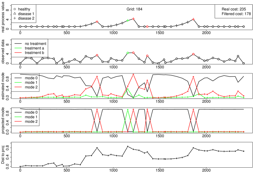
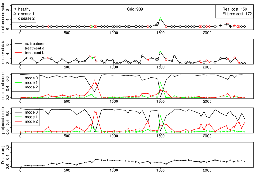
Figure 5: Trajectories for $L_{2}$ distance.

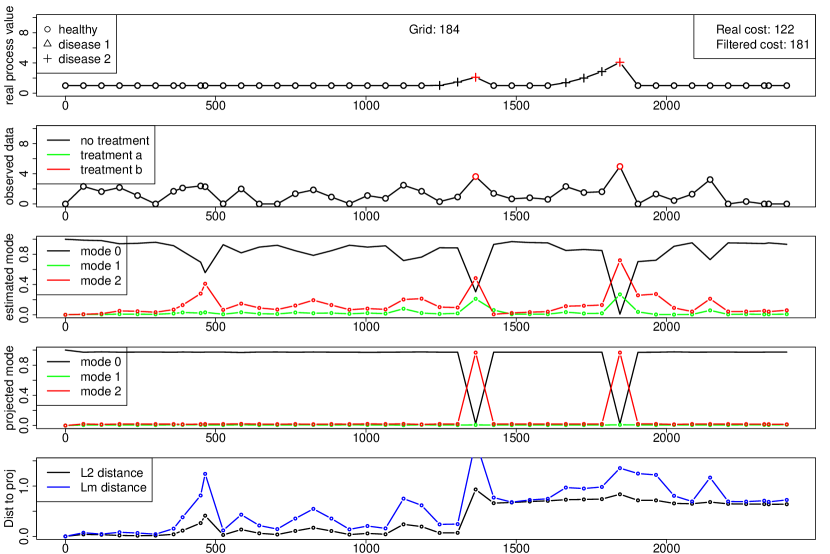
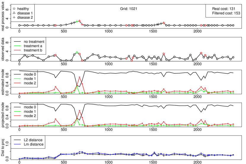
Figure 6: Trajectories for $L_{m}$ distance.

E.5 Choice of $\hat{\Psi}$ or $\bar{\Psi}$ in practice

The discretization strategy lead to a Markov kernel $\hat{R}^{\prime}$ on $\bar{\mathbb{X}}^{\prime}$ to which can be associated a Markov chain $\hat{\Psi}$. In theory, the dynamic programming algorithm operates on this Markov chain, and error bounds from the main theorem are computed accordingly. This should imply that at iteration $k$, filter $\bar{\Psi}_{k}$ is computed from the new observation and the current filter $\hat{\Psi}_{k-1}$, then projected on $\Gamma$ to identify the optimal decision. Then this projection $\hat{\Psi}_{k}=p_{|\Gamma}(\bar{\Psi}_{k})$ is saved as current filter for the next observation.

In practice, this implies that the projection error $\hat{\Psi}_{k}-\bar{\Psi}_{k}$ is propagated through the dynamic programming recursion. We propose instead to save $\bar{\Psi}_{k}$ as current filter for the next iteration, i.e. the filter at iteration $k+1$ will be computed using $Y_{k+1}$ and $\bar{\Psi}_{k}$. We do not propose any error bound on this practical strategy, and there is no guarantee that this should lead to better results, as projection errors on $\Gamma$ may sometimes compensate previous errors. However in our simulation studies we have observed a significant difference between the strategies, as illustrated in table 10 (grid $1021$ with $Lm$ distance).
One can note that the estimated cost is identical in the visit choice framework between filter $\bar{\Psi}$ and $\hat{\Psi}$ as they correspond to how grids were calibrated, but in practice the real cost is lower with $\bar{\Psi}$ as the latter is closer to the true data.

Table 10: Choice of $\hat{\Psi}$ or $\bar{\Psi}$ as current filter

			$\bar{\Psi}$		$\hat{\Psi}$
	Visits	$\hat{v}_{0}$	real cost (sd)	est. cost (sd)	real cost (sd)	est. cost (sd)
	OS	132.43	136.96 (3.97)	134.8 (0.75)	161.38 (7.2)	134.82 (0.96)
Grid	FD-15	253.28	214.29 (1.67)	215.83 (0.78)	227.84 (3.13)	264.19 (2.31)
1231	FD-60	163.57	143.02 (5.29)	141.8 (1.05)	163.19 (7.29)	165.22 (1.05)

References

• [1] Almudevar, A. (2001). A dynamic programming algorithm for the optimal control of piecewise deterministic markov processes. SIAM Journal on Control and Optimization 40, 525–539.
• [2] Bäuerle, N. and Lange, D. (2018). Optimal control of partially observable piecewise deterministic Markov processes. SIAM J. Control Optim. 56, 1441–1462.
• [3] Bäuerle, N. and Rieder, U. (2011). Markov decision processes with applications to finance. Universitext. Springer, Heidelberg.
• [4] Brandejsky, A., de Saporta, B. and Dufour, F. (2013). Optimal stopping for partially observed piecewise-deterministic Markov processes. Stochastic Process. Appl. 123, 3201–3238.
• [5] Calvia, A. (2020). Stochastic filtering and optimal control of pure jump markov processes with noise-free partial observation. ESAIM: Control, Optimisation and Calculus of Variations 26, 25.
• [6] Cleynen, A. and de Saporta, B. (2018). Change-point detection for piecewise deterministic markov processes. Automatica 97, 234–247.
• [7] Costa, O. and Dufour, F. (2013). Continuous average control of piecewise deterministic Markov processes. SpringerBriefs in Mathematics. Springer, New York.
• [8] Costa, O. and Raymundo, C. (2000). Impulse and continuous control of piecewise deterministic markov processes. Stochastics and Stochastic Reports 70, 75–107.
• [9] Costa, O. L. and Davis, M. (1989). Impulse control of piecewise-deterministic processes. Mathematics of Control, Signals and Systems 2, 187–206.
• [10] Davis, M. (1984). Piecewise-deterministic Markov processes: a general class of nondiffusion stochastic models. J. Roy. Statist. Soc. Ser. B 46, 353–388. With discussion.
• [11] Davis, M. (1993). Markov models and optimization vol. 49 of Monographs on Statistics and Applied Probability. Chapman & Hall, London.
• [12] de Saporta, B. and Dufour, F. (2012). Numerical method for impulse control of piecewise deterministic Markov processes. Automatica 48, 779–793.
• [13] de Saporta, B., Dufour, F. and Geeraert, A. (2017). Optimal strategies for impulse control of piecewise deterministic markov processes. Automatica 77, 219–229.
• [14] de Saporta, B., Dufour, F. and Zhang, H. (2016). Numerical methods for simulation and optimization of piecewise deterministic Markov processes. Mathematics and Statistics Series. ISTE, London; John Wiley & Sons, Inc., Hoboken, NJ. Application to reliability.
• [15] Dempster, M. and Ye, J. (1995). Impulse control of piecewise deterministic Markov processes. Ann. Appl. Probab. 5, 399–423.
• [16] Dufour, F., Horiguchi, M. and Piunovskiy, A. (2016). Optimal impulsive control of piecewise deterministic markov processes. Stochastics 88, 1073–1098.
• [17] Piunovskiy, A., Plakhov, A., Torres, D. F. and Zhang, Y. (2019). Optimal impulse control of dynamical systems. SIAM Journal on Control and Optimization 57, 2720–2752.