The stickiness property
for antisymmetric nonlocal minimal graphs

Abstract.

We show that arbitrarily small antisymmetric perturbations of the zero function are sufficient to produce the stickiness phenomenon for planar nonlocal minimal graphs (with the same quantitative bounds obtained for the case of even symmetric perturbations, up to multiplicative constants).

In proving this result, one also establishes an odd symmetric version of the maximum principle for nonlocal minimal graphs, according to which the odd symmetric minimizer is positive in the direction of the positive bump and negative in the direction of the negative bump.

1. Introduction

Nonlocal minimal surfaces were introduced in [MR2675483] as minimizers of a fractional perimeter functional with respect to some given external datum. As established in [MR3516886], when the external datum is a graph in some direction, so is the whole minimizer, hence it is also common to consider the case of nonlocal minimal graphs, i.e. of nonlocal minimal surfaces which possess a graphical structure.

Nonlocal minimal graphs exhibit a quite peculiar phenomenon, discovered in [MR3596708], called “stickiness”. Roughly speaking, different from the classical minimal surfaces, in the fractional setting remote interactions are capable of producing boundary discontinuities, which in turn are complemented by boundary divergence of the derivative of the nonlocal minimal graph: more specifically, boundary discontinuities of nonlocal minimal graphs are equivalent to the divergence at the boundary of the first derivative of the graph, see [MR4104542, Corollary 1.3], and this can also be interpreted as a “butterfly effect”, since a small perturbation of the boundary datum not only produces a small discontinuity of the graph at the boundary but it also forces the slope of the graph at the boundary to shift at once from a finite value (even zero) to infinity, see [MR4096831, Figure 3].

We focus here on the case in which the ambient space is of dimension $2$: this is indeed the simplest possible stage to detect interesting geometric patterns and, differently from the classical case, it already provides a number of difficulties since in the nonlocal framework segments are in general not the boundary of nonlocal minimal objects. Also, in the plane the stickiness phenomenon is known to be essentially “generic” with respect to the external datum, see [MR4104542], in the sense that boundary discontinuities and boundary singularities for the derivatives can be produced by arbitrarily small perturbations of a given external datum. In particular, these behaviors can be obtained by arbitrarily small perturbations of the flat case in which the external datum is, say, the subgraph of the function which is identically zero.

See also [MR4178752] for an analysis of nonlocal minimal graphs in dimension $3$, and [MR3926519, MR4184583, 2020arXiv201000798D] for other examples of stickiness.

Up to now, all the examples of stickiness in the setting of graphs were constructed by using “one side bumps” in the perturbation (for instance, adding suitable positive bumps to the zero function, or to a given function outside a vertical slab). In this paper, we construct examples of stickiness in which the datum is antisymmetric. In a nutshell, we will consider arbitrarily small perturbations of the zero function by bumps possessing odd symmetry: in this case, in principle, one may fear that the effects of equal and opposite bumps would cancel each other and prevent the stickiness phenomenon to occur, but we will instead establish that the stickiness phenomenon is persistent also in this class of antisymmetric perturbations of the flat case.

Also, we provide quantitative bounds on the resulting boundary discontinuity which turn out to be as good as the ones available for positive bumps (up to multiplicative constants).

The mathematical notation used in this paper goes as follows. Given $s\in(0,1)$, $a<b$ and $u_{0}\in C(\mathbb{R})$, we say that $u\in L^{\infty}_{\rm loc}(\mathbb{R})$ is an $s$-minimal graph in $(a,b)$ if:

• $u(x)=u_{0}(x)$ for every $x\in\mathbb{R}\setminus(a,b)$,

• for every $L>\|u\|_{L^{\infty}((a,b))}$ and every measurable function $v:\mathbb{R}\to\mathbb{R}$ such that $|v(x)|\leqslant L$ for all $x\in(a,b)$ we have that

  $$\mbox{\rm{Per}}_{s}(E_{u},\Omega_{L})\leqslant\mbox{\rm{Per}}_{s}(E_{v},\Omega_{L})$$

  where

  $$E_{u}:=\big{\{}(x,y)\in\mathbb{R}^{2}{\mbox{ s.t. }}y<u(x)\big{\}},$$

  $$E_{v}:=\big{\{}(x,y)\in\mathbb{R}^{2}{\mbox{ s.t. }}y<v(x)\big{\}},$$

  $$\Omega_{L}:=(a,b)\times(-L,L),$$

  $$\mbox{\rm{Per}}_{s}(E,\Omega):={\mathcal{L}}_{s}(E\cap\Omega,E^{c}\cap\Omega)+{\mathcal{L}}_{s}(E\cap\Omega,E^{c}\cap\Omega^{c})+{\mathcal{L}}_{s}(E\cap\Omega^{c},E^{c}\cap\Omega),$$

  $$\Omega^{c}:=\mathbb{R}^{2}\setminus\Omega$$

  and $${\mathcal{L}}_{s}(A,B):=\iint_{A\times B}\frac{dX\,dY}{|X-Y|^{2+s}}.$$

See Figure 1 for a sketch of the interactions detected by the definition above. See also [MR4279395] for further information about nonlocal minimal graphs and in particular Theorem 1.11 there for existence and uniqueness results for nonlocal minimal graphs.

We also recall that, while the minimizers of the classical perimeter have vanishing mean curvature, a minimizer $E$ in $\Omega$ of the fractional perimeter has vanishing fractional mean curvature, in the sense that, for every $P\in\Omega\cap(\partial E)$,

$$\int_{\mathbb{R}^{2}}\frac{\chi_{\mathbb{R}^{2}\setminus E}(X)-\chi_{E}(X)}{|X-P|^{2+s}}\,dX=0.$$

Here above and in the sequel, the singular integral is intended in the Cauchy principal value sense and the above equation reads in the sense of viscosity, see [MR2675483, Theorem 5.1] for full details.

Numerical examples of the stickiness properties have recently been provided by [MR3982031, MR4294645]. The theory of nonlocal minimal surfaces also presents a number of interesting offsprings, such as regularity theory [MR3090533, MR3107529, MR3331523, MR3680376, MR3798717, MR3934589, MR3981295, MR4050198, MR4116635], isoperimetric problems and the study of constant mean curvature surfaces [MR2799577, MR3322379, MR3412379, MR3485130, MR3744919, MR3836150, MR3881478], geometric evolution problems [MR2487027, MR3156889, MR3713894, MR3778164, MR3951024], front propagation problems [MR2564467], phase transition problems [MR3133422], etc.

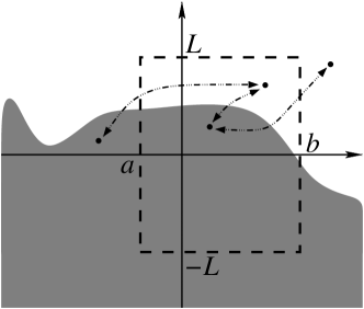
Figure 1. The interactions contributing to the fractional perimeter.

Having formalized the setting in which we work, we can now state our result about the stickiness phenomenon in the antisymmetric setting as an arbitrarily small perturbation of the flat case:

Theorem 1.1.

Let $\epsilon_{0}>0$, $\bar{C}>0$, $d>d_{0}>0$ and $h>0$, with

(1.1) $$\frac{h^{2+s}}{(h^{2}+2)^{\frac{2+s}{2}}}>\frac{2\bar{C}}{(1+s){\left(d-d_{0}\right)^{1+s}}}.$$

Then, there exist $C>0$ and $\eta_{0}\in(0,1)$, depending only on $s$, $\epsilon_{0}$, $\bar{C}$, $d$, $d_{0}$ and $h$, such that if $\eta\in(0,\eta_{0}]$ the following claim holds true.

Let $u_{0}\in C(\mathbb{R})$. Assume that

(1.2) $$u_{0}(x)=0\quad{\mbox{ for all }}x\in(d,d+h),$$

(1.3) $$u_{0}(x)\leqslant 0\quad{\mbox{ for all }}x\in(d,+\infty),$$

(1.4) $$\|u_{0}\|_{L^{\infty}(\mathbb{R})}\leqslant\bar{C}\eta,$$

(1.5) $$u_{0}(x)=-u_{0}(-x)\quad{\mbox{ for all }}x\in(d,+\infty)$$

and

(1.6) $$\int_{-\infty}^{-d-h}\frac{u_{0}(x)}{|d_{0}-d-x|^{2+s}}\,dx\geqslant\eta.$$

Let $u$ be the $s$-minimal graph with $u=u_{0}$ in $\mathbb{R}\setminus(-d,d)$.

Then,

(1.7) $$u(x)=-u(-x)\quad{\mbox{ for all }}x\in(-\infty,+\infty),$$

(1.8) $$u(x)\geqslant 0\quad{\mbox{ for all }}x\in(-\infty,0],$$

(1.9) $$u(x)\leqslant 0\quad{\mbox{ for all }}x\in[0,+\infty)$$

and, for every $x\in(-d,-d+d_{0})$,

(1.10) $$u(x)\geqslant\frac{\eta^{\frac{2+\epsilon_{0}}{1-s}}}{C}.$$

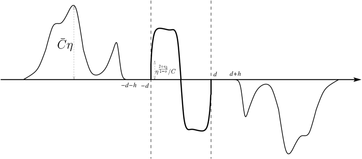
Figure 2. The antisymmetric stickiness phenomenon, as given in Theorem 1.1.

See Figure 2 for a sketch of the geometric scenario described in Theorem 1.1. Interestingly, the antisymmetric stickiness power $\frac{2+\epsilon_{0}}{1-s}$ in (1.10) is the same as the one detected in [MR3596708, Theorem 1.4] for the even symmetric case (hence, the antisymmetric case appears to be also quantitatively in agreement with the even symmetric configurations, up to multiplicative constants).

Notice also that condition (1.1) simply states that $d$ is sufficiently large with respect to other structural parameters. For instance, one can take

$$\bar{C}:=2^{2+s}(1+s),\qquad d:=3^{\frac{2+s}{2(1+s)}}2^{\frac{3+s}{1+s}}+2\qquad d_{0}:=1\quad{\mbox{ and }}\quad h:=1.$$

Notice that with this choice of parameters, condition (1.1) is satisfied. We also define

$$d_{1}:=2\left(\left(\frac{10}{9}\right)^{\frac{1}{1+s}}-1\right)\quad{\mbox{ and }}\quad d_{2}:=2\left(10^{\frac{1}{1+s}}-1\right),$$

and we take $u_{0}\in C(\mathbb{R})$ satisfying (1.2), (1.3), (1.4) and (1.5), and such that

$$u_{0}\geqslant\bar{C}\eta\chi_{(-d-h-d_{2},-d-h-d_{1})}\quad{\mbox{ in }}(-\infty,-d).$$

With this choice of $u_{0}$ we have that (1.6) is also satisfied. Indeed, using the change of variable $z:=d_{0}-d-x$,

$$\int_{-\infty}^{-d-h}\frac{u_{0}(x)}{|d_{0}-d-x|^{2+s}}\,dx\geqslant\int_{-d-h-d_{2}}^{-d-h-d_{1}}\frac{u_{0}(x)}{|d_{0}-d-x|^{2+s}}\,dx$$

$$\qquad\qquad\geqslant\int_{-d-h-d_{2}}^{-d-h-d_{1}}\frac{\bar{C}\eta}{|d_{0}-d-x|^{2+s}}\,dx=\bar{C}\eta\int_{d_{0}+h+d_{1}}^{d_{0}+h+d_{2}}\frac{dz}{z^{2+s}}$$

$$\qquad\qquad=\frac{\bar{C}\eta}{1+s}\left[\frac{1}{(d_{0}+h+d_{1})^{1+s}}-\frac{1}{(d_{0}+h+d_{2})^{1+s}}\right]$$

$$\qquad\qquad=2^{2+s}\eta\left(\frac{1}{2^{1+s}\frac{10}{9}}-\frac{1}{2^{1+s}10}\right)=2\eta\frac{8}{10}>\eta,$$

as desired.

We also point out that condition (1.2) can be relaxed and is taken here mostly to emphasize that “instability” (as embodied by the stickiness phenomenon) arises in the case of nonlocal minimal surfaces even when the external datum is, near the boundary of the domain, as regular, as “stable” and “as flat” as one wishes: more specifically, the stickiness that we detect is not due to possible oscillatory behaviors of the external datum near the domain of reference, but is merely the outcome of long-distance interactions.

As for condition (1.6), its meaning is, roughly speaking, that the external datum presents a “positive bump” at the left (which corresponds to a “negative bump” at the right). The role of the parameter $\eta$ is to give an explicit quantification of this bump: this quantification is given in an integral form, since we want to weigh the “size” of the bump (given by the numerator of the integrand on the left hand side of (1.6)) against the interaction kernel, because this is, in a sense, the “long-distance force” exerted by the bump on the nonlocal minimal graph.

The gist of the proof of Theorem 1.1 is to employ the auxiliary function constructed in [MR3596708, Corollary 7.2]. This barrier will be suitably scaled and placed near the left end of the reference domain to show that the nonlocal minimal graph under consideration must be “lifted up”. From a quantitative point of view, this localized barrier presents a nonlocal mean curvature which has possibly a “wrong sign” somewhere, but this sign discrepancy is controlled by a small quantity (roughly speaking, playing the role of $\eta$ in the statement of Theorem 1.1, up to a convenient choice of a multiplicative constant). With this respect, the external bump in condition (1.6) compensates the “small sign discrepancy” of this localized barrier. That is, roughly speaking, the positive bump on the left will produce an advantageous term, while the negative bump on the right and the modification needed to lower the barrier in the negativity region of $u$ will produce a disadvantageous term of the same order. Thus, playing around with constants, one detects a natural structure assuring that the advantageous term is greater than the sum of the initial error on the nonlocal mean curvature, the contribution of the negative bump and the error coming from the barrier modification.

In this procedure, however, an additional difficulty arises, since in our framework the solution will cross the horizontal axis. For this reason, the previous barrier (which is designed to be a small upward bump) cannot be exploited as it is and needs to be modified to stay below the “expected” negative regions of the minimizer.

To this end, we first need to identify a “safe region near the boundary” for the minimizer, that is an interval of well-determined length in which one can be sure that the solution is positive: once this is accomplished, it will be possible to slide from below the appropriate barrier whose positive portion occurs precisely in the above safe region. A graphical sketch of such a barrier will be given in Figure 5.

In view of these comments, to identify the safe region near the boundary and perform the proof of Theorem 1.1, we establish a result of general interest, which can be seen as a “maximum principle for antisymmetric $s$-minimal graphs”. For our purposes, the safe region will correspond to the positive values of $u$, which, thanks to this antisymmetric maximum principle, extends to the whole interval $(-d,0)$.

Roughly speaking, the classical maximum principle for $s$-minimal graphs (see e.g. [MR2675483, MR3516886]) states that if the external data of an $s$-minimal graph are positive (or negative) then so is the $s$-minimal graph. Here we deal with an antisymmetric configuration, hence it is not possible for the external data of an $s$-minimal graph to have a sign (except in the trivial case of identically zero datum, which produces the identically zero $s$-minimizer). Hence, the natural counterpart of the maximum principle in the antisymmetric framework is to assume that the external datum “on one side” has a sign, thus forcing the external datum on the other side to have the opposite sign. Under this assumption, we show that the corresponding $s$-minimal graph maintains the antisymmetry and sign properties of the datum, according to the following result:

Theorem 1.2.

Let $d$, $h>0$. Let $u:\mathbb{R}\to\mathbb{R}$ be an $s$-minimal graph in $(-d,d)$, with $u\in C(-\infty,-d)\cap C^{1,\frac{1+s}{2}}(-d-h,-d)$. Assume that

(1.11) $$u(x)=-u(-x)\quad{\mbox{ for all }}x\in(d,+\infty)$$

and that

(1.12) $$u(x)\leqslant 0\quad{\mbox{ for all }}x\in(d,+\infty).$$

Then,

(1.13) $$u(x)=-u(-x)\quad{\mbox{ for all }}x\in(-\infty,+\infty),$$

(1.14) $$u(x)\geqslant 0\quad{\mbox{ for all }}x\in(-\infty,0]$$

and

(1.15) $$u(x)\leqslant 0\quad{\mbox{ for all }}x\in[0,+\infty).$$

Figure 3. The maximum principle for antisymmetric nonlocal minimal graphs, as given in Theorem 1.2.

See Figure 3 for a sketch of the configuration detected in Theorem 1.2.

The proofs of Theorems 1.1 and 1.2 are contained in Sections 2 and 3, respectively. As a matter of fact, Theorem 1.2 will follow from a more general statement valid for supersolutions, given in the forthcoming Lemma 3.1.

Section 4 contains a discussion about the proof of the antisymmetric maximum principle, compared with the existing theory focused on the antisymmetric maximum principle for the fractional Laplacian and linear nonlocal operators.

2. Proof of Theorem 1.1

We give here the proof of Theorem 1.1. At this stage, we freely use the antisymmetric maximum principle in Theorem 1.2, whose proof is postponed to Section 3.

We also use the notation $X=(x,y)$ to denote points in $\mathbb{R}^{2}$, with $x$, $y\in\mathbb{R}$.

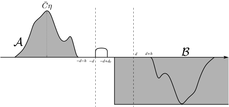
Figure 4. The sets ${\mathcal{A}}$ and ${\mathcal{B}}$ in the proof of Theorem 1.1.

The proof of Theorem 1.1 consists of five steps.

Step 1: Construction of the barrier $U_{\delta}$. Let $\epsilon_{0}>0$. Given $\delta\in(0,1)$ sufficiently small, we apply [MR3596708, Corollary 7.2] and we find a set $H_{\delta}\subset\mathbb{R}^{2}$ that contains the halfplane $\mathbb{R}\times(-\infty,0)$ and is contained in the halfplane $\mathbb{R}\times(-\infty,\delta)$, such that

$$\left\{(x,y)\in H_{\delta}{\mbox{ s.t. }}x\in(-\infty,-d)\cup\left(-d+d_{0},+\infty\right)\right\}$$

$$\qquad=\left\{(x,y)\in\mathbb{R}^{2}{\mbox{ s.t. }}x\in(-\infty,-d)\cup\left(-d+d_{0},+\infty\right){\mbox{ and }}y\in(-\infty,0)\right\},$$

with

(2.1) $$\begin{split}&\left\{(x,y)\in H_{\delta}{\mbox{ s.t. }}x\in\left(-d,-d+d_{0}\right)\right\}\\ &\qquad\supseteq\left\{(x,y)\in\mathbb{R}^{2}{\mbox{ s.t. }}x\in\left(-d,-d+d_{0}\right)\times\left(-\infty,\delta^{\frac{2+\epsilon_{0}}{1-s}}\right)\right\}\end{split}$$

and satisfying, for each $P=(p,q)\in\partial H_{\delta}$ with $p\in\left(-d,-d+d_{0}\right)$,

(2.2) $$\int_{\mathbb{R}^{2}}\frac{\chi_{\mathbb{R}^{2}\setminus H_{\delta}}(X)-\chi_{H_{\delta}}(X)}{|X-P|^{2+s}}\,dX\leqslant C\delta,$$

for some constant $C>0$ depending only on $s$, $\epsilon_{0}$ and $d$.

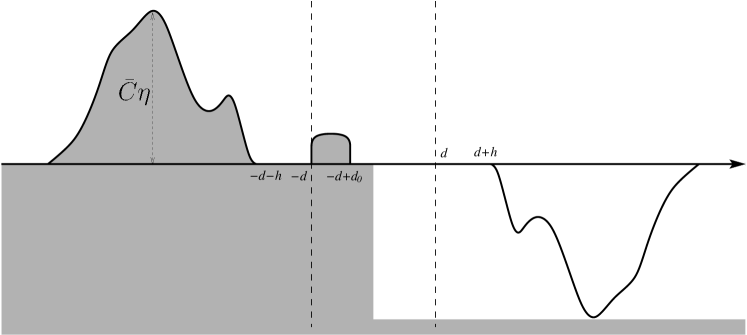
Figure 5. The set $U_{\delta}$ used in the proof of Theorem 1.1.

The strategy will be to take

(2.3) $$\eta:=C_{\star}\delta$$

in the statement of Theorem 1.1, with $C_{\star}>0$ to be sufficiently large. We let

$${\mathcal{A}}:=\big{\{}(x,y)\in\mathbb{R}^{2}{\mbox{ s.t. }}x\in(-\infty,-d){\mbox{ and }}0<y<u_{0}(x)\big{\}},$$

$${\mathcal{B}}:=\big{\{}(x,y)\in\mathbb{R}^{2}{\mbox{ s.t. }}x\in(0,+\infty){\mbox{ and }}-\bar{C}\eta<y<0\big{\}}$$

and $$U_{\delta}:=(H_{\delta}\cup{\mathcal{A}})\setminus{\mathcal{B}},$$

see Figure 4 to visualize the sets ${\mathcal{A}}$ and ${\mathcal{B}}$ and Figure 5 to visualize the set $U_{\delta}$.

Step 2: Estimates for some integrals appearing in the nonlocal mean curvature of $U_{\delta}$. We observe that ${\mathcal{A}}\cap H_{\delta}=\varnothing$ and ${\mathcal{B}}\subset H_{\delta}$. Consequently,

$$\chi_{U_{\delta}}=\chi_{H_{\delta}}+\chi_{{\mathcal{A}}}-\chi_{{\mathcal{B}}}$$

and $$\chi_{\mathbb{R}^{2}\setminus U_{\delta}}=\chi_{\mathbb{R}^{2}\setminus(H_{\delta}\cup{\mathcal{A}})}+\chi_{{\mathcal{B}}}\leqslant\chi_{\mathbb{R}^{2}\setminus H_{\delta}}+\chi_{{\mathcal{B}}}.$$

From this and the inequality for $H_{\delta}$ in (2.2), we have that, for all $P=(p,q)\in\partial H_{\delta}$ with $p\in\left(-d,-d+d_{0}\right)$,

(2.4) $$\begin{split}&\int_{\mathbb{R}^{2}}\frac{\chi_{\mathbb{R}^{2}\setminus U_{\delta}}(X)-\chi_{U_{\delta}}(X)}{|X-P|^{2+s}}\,dX\\ &\qquad\leqslant\int_{\mathbb{R}^{2}}\frac{\chi_{\mathbb{R}^{2}\setminus H_{\delta}}(X)+\chi_{{\mathcal{B}}}(X)-\big{(}\chi_{H_{\delta}}(X)+\chi_{{\mathcal{A}}}(X)-\chi_{{\mathcal{B}}(X)}\big{)}}{|X-P|^{2+s}}\,dX\\ &\qquad\leqslant C\delta+2\int_{{\mathcal{B}}}\frac{dX}{|X-P|^{2+s}}-\int_{{\mathcal{A}}}\frac{dX}{|X-P|^{2+s}}.\end{split}$$

We note that, for all $P=(p,q)\in\partial H_{\delta}$ with $p\in\left(-d,-d+d_{0}\right)$,

$$\int_{{\mathcal{B}}}\frac{dX}{|X-P|^{2+s}}\leqslant\int_{{\mathcal{B}}}\frac{dX}{|x-p|^{2+s}}=\bar{C}\eta\int_{0}^{+\infty}\frac{dx}{|x-p|^{2+s}}=\bar{C}\eta\int_{0}^{+\infty}\frac{dx}{(x-p)^{2+s}}$$

$$\qquad\leqslant\bar{C}\eta\int_{0}^{+\infty}\frac{dx}{\left(x+d-d_{0}\right)^{2+s}}=\frac{\bar{C}\eta}{(1+s){\left(d-d_{0}\right)^{1+s}}}=\frac{\bar{C}C_{\star}\delta}{(1+s){\left(d-d_{0}\right)^{1+s}}}.$$

This and (2.4) yield that

(2.5) $$\int_{\mathbb{R}^{2}}\frac{\chi_{\mathbb{R}^{2}\setminus U_{\delta}}(X)-\chi_{U_{\delta}}(X)}{|X-P|^{2+s}}\,dX\leqslant C\delta+\frac{2\bar{C}C_{\star}\delta}{(1+s){\left(d-d_{0}\right)^{1+s}}}-\int_{{\mathcal{A}}}\frac{dX}{|X-P|^{2+s}}.$$

Step 3: Estimate for the third term in (2.5). Let us now estimate the last integral in (2.5). By (1.4), if $X=(x,y)\in{{\mathcal{A}}}$ and $P=(p,q)\in\partial H_{\delta}$ with $p\in\left(-d,-d+d_{0}\right)$,

$$|y-q|\leqslant|y|+|q|\leqslant 1+\delta\leqslant 2.$$

Moreover, owing to the assumptions on $u$ in (1.2) and (1.5), for all $x\in(-d-h,-d)$ we have that $u_{0}(x)=-u_{0}(-x)=0$.

Accordingly, if $X=(x,y)\in{{\mathcal{A}}}$ then $x\leqslant-d-h$. As a result, if $X=(x,y)\in{{\mathcal{A}}}$ and $P=(p,q)\in\partial H_{\delta}$ with $p\in\left(-d,-d+d_{0}\right)$,

$$\begin{split}&|x-p|\geqslant\min\big{\{}|x-p|,\,|x+p|\big{\}}\geqslant\min\big{\{}p-x,\,-p-x\big{\}}\\ &\qquad\geqslant\min\left\{-d-(-d-h),\,d-d_{0}-(-d-h)\right\}=\min\left\{h,2d-d_{0}+h\right\}=h.\end{split}$$

From these remarks we obtain that

$$|X-P|=|x-p|\sqrt{1+\frac{|y-q|^{2}}{|x-p|^{2}}}\leqslant|x-p|\sqrt{1+\frac{2}{h^{2}}}=|x-p|\sqrt{\frac{h^{2}+2}{h^{2}}}.$$

Hence,

(2.6) $$\begin{split}&\int_{{\mathcal{A}}}\frac{dX}{|X-P|^{2+s}}\geqslant\frac{h^{2+s}}{(h^{2}+2)^{\frac{2+s}{2}}}\int_{{\mathcal{A}}}\frac{dX}{|x-p|^{2+s}}\\ &\qquad\qquad=\frac{h^{2+s}}{(h^{2}+2)^{\frac{2+s}{2}}}\int_{-\infty}^{-d}\frac{u_{0}(x)}{|x-p|^{2+s}}\,dx=\frac{h^{2+s}}{(h^{2}+2)^{\frac{2+s}{2}}}\int_{-\infty}^{-d-h}\frac{u_{0}(x)}{|x-p|^{2+s}}\,dx.\end{split}$$

Since, if $p\in\left(-d,-d+d_{0}\right)$ and $x\in(-\infty,-d-h)$,

$$|x-p|=p-x\leqslant-d+d_{0}-x=|d_{0}-d-x|,$$

we deduce from (2.6) that

$$\int_{{\mathcal{A}}}\frac{dX}{|X-P|^{2+s}}\geqslant\frac{h^{2+s}}{(h^{2}+2)^{\frac{2+s}{2}}}\int_{-\infty}^{-d-h}\frac{u_{0}(x)}{|d_{0}-d-x|^{2+s}}\,dx.$$

This, the integral assumption on $u_{0}$ in (1.6) and the definition of $\eta$ in (2.3) give that

$$\int_{{\mathcal{A}}}\frac{dX}{|X-P|^{2+s}}\geqslant\frac{h^{2+s}\eta}{(h^{2}+2)^{\frac{2+s}{2}}}=\frac{C_{\star}h^{2+s}\delta}{(h^{2}+2)^{\frac{2+s}{2}}}.$$

Plugging this information into (2.5) we infer that

(2.7) $$\int_{\mathbb{R}^{2}}\frac{\chi_{\mathbb{R}^{2}\setminus U_{\delta}}(X)-\chi_{U_{\delta}}(X)}{|X-P|^{2+s}}\,dX\leqslant C\delta+\frac{2\bar{C}C_{\star}\delta}{(1+s){\left(d-d_{0}\right)^{1+s}}}-\frac{C_{\star}h^{2+s}\delta}{(h^{2}+2)^{\frac{2+s}{2}}}.$$

Step 4: Conclusion of the proof that $U_{\delta}$ is a subsolution. Now we define

$$\vartheta:=\frac{h^{2+s}}{(h^{2}+2)^{\frac{2+s}{2}}}-\frac{2\bar{C}}{(1+s){\left(d-d_{0}\right)^{1+s}}}$$

and we observe that $\vartheta>0$, owing to the relation between parameters in (1.1). Then, we deduce from (2.7) that

(2.8) $$\int_{\mathbb{R}^{2}}\frac{\chi_{\mathbb{R}^{2}\setminus U_{\delta}}(X)-\chi_{U_{\delta}}(X)}{|X-P|^{2+s}}\,dX\leqslant C\delta-C_{\star}\vartheta\delta\leqslant-\frac{C_{\star}\vartheta\delta}{2}<0,$$

as long as $C_{\star}$ is large enough.

Step 5: Sliding method and conclusion of the proof of Theorem 1.1. We can now use $U_{\delta}$ as a barrier for the sliding method. Specifically, by (1.4) and the maximum principle in [MR2675483], we know that $|u(x)|\leqslant\bar{C}\eta<1$ for all $x\in\mathbb{R}$ and therefore a downwards translation of $U_{\delta}$ with magnitude $1$, that we denote by $U_{\delta}-(0,1)$, is completely contained in $E_{u}:=\big{\{}(x,y)\in\mathbb{R}^{2}{\mbox{ s.t. }}y<u(x)\big{\}}$.

We then slide up till we reach a touching point: given $\tau\in(0,1]$, we notice that by construction no touching can occur between $E_{u}$ and $U_{\delta}-(0,\tau)$ at points with abscissa in $\mathbb{R}\setminus[-d,0]$. But these touching points cannot occur in $\left(-d+d_{0},0\right]$ either, thanks to the sign assumption in (3.5). And they cannot occur in $\left[-d,-d+d_{0}\right]$, thanks to (2.8) and the maximum principle in [MR2675483] (see also [MR4104542, Theorem 1.4]).

As a consequence, we have that $U_{\delta}\subseteq E_{u}$. By virtue of (2.1) and (2.3), this establishes (1.10).

Also, the claims in (1.7), (1.8) and (1.9) follow from (1.13), (3.5) and (3.6). $\Box$

3. Proof of Theorem 1.2

We now provide a more general antisymmetric maximum principle valid for supersolutions, from which Theorem 1.2 will plainly follow by using also other results already available in the literature.

Lemma 3.1.

Let $d>0$. Let $u:\mathbb{R}\to\mathbb{R}$, with $u\in C([-d,0])\cap C^{1,\alpha}((-d,0])$ for some $\alpha\in\left(\frac{1+s}{2},1\right)$.

Let also

$$E:=\big{\{}(x,y)\in\mathbb{R}^{2}{\mbox{ s.t. }}y<u(x)\big{\}}.$$

Assume that, for all $P=(p,u(p))$ with $p\in(-d,0]$, we have

(3.1) $$\int_{\mathbb{R}^{2}}\frac{\chi_{\mathbb{R}^{2}\setminus E}(X)-\chi_{E}(X)}{|X-P|^{2+s}}\,dX\geqslant 0.$$

Suppose also that

(3.2) $$u(-d)>\min_{[-d,0]}u,$$

that

(3.3) $$u(x)=-u(-x)\quad{\mbox{ for all }}x\in(0,+\infty)$$

and that

(3.4) $$u(x)\leqslant 0\quad{\mbox{ for all }}x\in(d,+\infty).$$

Then,

(3.5) $$u(x)\geqslant 0\quad{\mbox{ for all }}x\in(-\infty,0]$$

and

(3.6) $$u(x)\leqslant 0\quad{\mbox{ for all }}x\in[0,+\infty).$$

Proof.

It suffices to show that $u\geqslant 0$ in $(-\infty,0]$, that is (3.5), since (3.6) would then follow from the odd symmetry of $u$ given by (3.3) and the nonnegativity of $u$ in $(-\infty,0]$ in (3.5).

To prove (3.5) we argue by contradiction and assume that (3.5) is violated. Note that

(3.7) if $$x\in(-\infty,-d) u(x)=-u(-x)\geqslant 0$$ then ,

thanks to the assumptions on $u$ in (3.3) and (3.4).

This, the continuity of $u$ in $[-d,0]$ and our contradictory assumption give that there exists $p\in[-d,0]$ such that

(3.8) $$u(p)=\min_{[-d,0]}u<0.$$

We claim that

(3.9) $$p\in(-d,0).$$

Indeed, since $u(0)=-u(0)$ by the odd symmetric of $u$ in (3.3), we have that $u(0)=0$ and accordingly $p\neq 0$. This and (3.2) lead to (3.9), as desired.

By (3.9), we know that the supersolution condition (3.1) holds true for $P:=(p,u(p))$.

We will now reach a contradiction by showing that (3.1) is violated, since “the set $E$ is too large”. To this end, we consider the sets

(3.10) $$\begin{split}&F_{-}:=\big{\{}x\in\mathbb{R}{\mbox{ s.t. }}u(x)<u(p)\big{\}}\\ {\mbox{and }}\quad&F_{+}:=\big{\{}x\in\mathbb{R}{\mbox{ s.t. }}u(x)>-u(p)\big{\}},\end{split}$$

see Figure 6 (notice in particular that the sets $F_{-}$ and $F_{+}$ are given by the bold intervals along the horizontal axis in Figure 6).

Figure 6. The geometry involved in the proof of Lemma 3.1: detection of cancellations via isometric regions. In particular, the sets $F_{-}$ and $F_{+}$ in (3.10) are given by the bold intervals along the horizontal axis.

We notice that, in light of (3.4), (3.7) and (3.8),

$$F_{-}\subseteq(0,+\infty)\quad{\mbox{ and }}\quad F_{+}\subseteq(-\infty,0).$$

Furthermore, by the odd symmetry of $u$ in (3.3), we have that

(3.11) $$x\in F_{-} -x\in F_{+}$$ if and only if .

The strategy now is based on the detection of suitable cancellations via isometric regions that correspond to the sets $F_{-}$ and $F_{+}$. The gist is to get rid of the contributions arising from the complement of $E$ below the line $\{y=u(p)\}$. For this, one has to use suitable transformations inherited from the geometry of the problem, such as an odd reflection through the origin, a vertical translation of magnitude $2u(p)$ and the reflection along the line $\{y=u(p)\}$. The use of these transformations will aim, on the one hand, at detecting isometric regions in $E$ which cancel the ones in the complement of $E$ in the integral computations, and, on the other hand, at maintaining a favorable control of the distance from the point $P$, since this quantity appears at the denominator of the integrands involved.

To employ this strategy, we use the notation $X=(x,y)$ and the transformation

$$\widetilde{X}=(\widetilde{x},\widetilde{y})=\widetilde{X}(X):=\big{(}-x,2u(p)-y\big{)}$$

and we claim that

(3.12) if $$x\geqslant 0 |X-P|\geqslant|\widetilde{X}-P|$$, then .

To check this, we observe that when $x\geqslant 0$ it follows that $xp\leqslant 0$ and therefore

$$|\widetilde{X}-P|^{2}-|X-P|^{2}$$

$$= \Big{|}\big{(}-x,2u(p)-y\big{)}-\big{(}p,u(p)\big{)}\Big{|}^{2}-\Big{|}(x,y)-\big{(}p,u(p)\big{)}\Big{|}^{2}$$

$$= \Big{|}\big{(}-x-p,u(p)-y\big{)}\Big{|}^{2}-\Big{|}\big{(}x-p,y-u(p)\big{)}\Big{|}^{2}$$

$$= (-x-p)^{2}-(x-p)^{2}$$

$$= 4xp$$

$$\leqslant 0,$$

which establishes (3.12).

Besides, we define

$$G:=\Big{\{}X=(x,y)\in\mathbb{R}^{2}\setminus E{\mbox{ s.t. $x\in F_{-}$ and $y<2u(p)-u(x)$}}\Big{\}}$$

and we claim that

(3.13) if $$X\in G \widetilde{X}\in E\cap\{\widetilde{x}\in F_{+}\}\cap\{-u(\widetilde{x})<\widetilde{y}<2u(p)+u(\widetilde{x})\}$$, then .

Indeed, if $X\in G$, by the odd symmetry in (3.3) we have that $y>u(x)=-u(-x)$ and accordingly

(3.14) $$\widetilde{y}=2u(p)-y<2u(p)+u(-x)=2u(p)+u(\widetilde{x}).$$

In particuar, $\widetilde{y}<u(\widetilde{x})$. From this, (3.11) and (3.14) we obtain that

(3.15) $$\widetilde{X}\in E\cap\{\widetilde{x}\in F_{+}\}\cap\{\widetilde{y}<2u(p)+u(\widetilde{x})\}.$$

Additionally,

$$\widetilde{y}=2u(p)-y>2u(p)-\big{(}2u(p)-u(x)\big{)}=u(x)=u(-\widetilde{x})=-u(\widetilde{x}).$$

Combining this with (3.15) we obtain (3.13), as desired.

Now, in light of (3.12) and (3.13), and observing that $d\widetilde{X}=dX$,

(3.16) $$\begin{split}&\int_{\mathbb{R}^{2}\cap\{x\in F_{-}\}\cap\{y<2u(p)-u(x)\}}\frac{\chi_{\mathbb{R}^{2}\setminus E}(X)}{|X-P|^{2+s}}\,dX\\ &\qquad=\int_{G}\frac{dX}{|X-P|^{2+s}}\leqslant\int_{G}\frac{dX}{|\widetilde{X}(X)-P|^{2+s}}\\ &\qquad\leqslant\int_{E\cap\{\widetilde{x}\in F_{+}\}\cap\{-u(\widetilde{x})<\widetilde{y}<2u(p)+u(\widetilde{x})\}}\frac{d\widetilde{X}}{|\widetilde{X}-P|^{2+s}}\\ &\qquad=\int_{\mathbb{R}^{2}\cap\{\widetilde{x}\in F_{+}\}\cap\{-u(\widetilde{x})<\widetilde{y}<2u(p)+u(\widetilde{x})\}}\frac{\chi_{E}(\widetilde{X})}{|\widetilde{X}-P|^{2+s}}\,d\widetilde{X}.\end{split}$$

Now we use the even reflection across the line $\{y=u(p)\}$, that is we define

(3.17) $$X_{*}=(x_{*},y_{*})=X_{*}(X):=\big{(}x,2u(p)-y\big{)}.$$

We notice that

(3.18) $$|X_{*}-P|=\Big{|}\big{(}x,2u(p)-y\big{)}-\big{(}p,u(p)\big{)}\Big{|}=\Big{|}\big{(}x-p,u(p)-y\big{)}\Big{|}=|X-P|.$$

As a result,

$$\int_{\mathbb{R}^{2}\cap\{x\in F_{-}\}\cap\{y>2u(p)-u(x)\}}\frac{\chi_{\mathbb{R}^{2}\setminus E}(X)}{|X-P|^{2+s}}\,dX\leqslant\int_{\mathbb{R}^{2}\cap\{x\in F_{-}\}\cap\{y>2u(p)-u(x)\}}\frac{dX}{|X-P|^{2+s}}$$

$$\quad=\int_{\mathbb{R}^{2}\cap\{x\in F_{-}\}\cap\{y>2u(p)-u(x)\}}\frac{dX}{|X_{*}(X)-P|^{2+s}}=\int_{\mathbb{R}^{2}\cap\{x\in F_{-}\}\cap\{y_{*}<u(x_{*})\}}\frac{dX_{*}}{|X_{*}-P|^{2+s}}$$

$$\qquad=\int_{\mathbb{R}^{2}\cap\{x\in F_{-}\}}\frac{\chi_{E}(X_{*})}{|X_{*}-P|^{2+s}}\,dX_{*}.$$

From this and (3.16), changing the names of the integration variables, we arrive at

$$\int_{\mathbb{R}^{2}\cap\{x\in F_{-}\}}\frac{\chi_{\mathbb{R}^{2}\setminus E}(X)}{|X-P|^{2+s}}\,dX$$

$$\qquad\leqslant\int_{\mathbb{R}^{2}\cap\{x\in F_{+}\}\cap\{-u(x)<y<2u(p)+u(x)\}}\frac{\chi_{E}(X)}{|X-P|^{2+s}}\,dX+\int_{\mathbb{R}^{2}\cap\{x\in F_{-}\}}\frac{\chi_{E}(X)}{|X-P|^{2+s}}\,dX,$$

that is

$$\int_{\mathbb{R}^{2}\cap\{x\in F_{-}\}}\frac{\chi_{\mathbb{R}^{2}\setminus E}(X)-\chi_{E}(X)}{|X-P|^{2+s}}\,dX\leqslant\int_{\mathbb{R}^{2}\cap\{x\in F_{+}\}\cap\{-u(x)<y<2u(p)+u(x)\}}\frac{\chi_{E}(X)}{|X-P|^{2+s}}\,dX.$$

Therefore,

(3.19) $$\begin{split}&\int_{\mathbb{R}^{2}\cap\{x\in F_{-}\cup F_{+}\}}\frac{\chi_{\mathbb{R}^{2}\setminus E}(X)-\chi_{E}(X)}{|X-P|^{2+s}}\,dX\\ \leqslant&\int_{\mathbb{R}^{2}\cap\{x\in F_{+}\}}\frac{\chi_{\mathbb{R}^{2}\setminus E}(X)-\chi_{E}(X)}{|X-P|^{2+s}}\,dX+\int_{\mathbb{R}^{2}\cap\{x\in F_{+}\}\cap\{-u(x)<y<2u(p)+u(x)\}}\frac{\chi_{E}(X)}{|X-P|^{2+s}}\,dX\\ =&\int_{\mathbb{R}^{2}\cap\{x\in F_{+}\}}\frac{\chi_{\mathbb{R}^{2}\setminus E}(X)}{|X-P|^{2+s}}\,dX-\int_{\mathbb{R}^{2}\cap\{x\in F_{+}\}\cap\{y\in(-\infty,-u(x))\cup(2u(p)+u(x),+\infty)\}}\frac{\chi_{E}(X)}{|X-P|^{2+s}}\,dX.\end{split}$$

Now, recalling the notation in (3.17), we note that

(3.20) if $$X\in(\mathbb{R}^{2}\setminus E)\cap\{x\in F_{+}\} X_{*}\in E\cap\{x_{*}\in F_{+}\}\cap\{y_{*}\in(-\infty,-u(x_{*}))\}$$, then .

Indeed, if $X$ is as above then, since $u(p)<0$,

(3.21) $$y_{*}=2u(p)-y<2u(p)-u(x)<-u(x)=-u(x_{*}).$$

Hence, since $u(x_{*})=u(x)>-u(p)>0$,

$$y_{*}<-u(x_{*})<u(x_{*}).$$

By gathering this and (3.21) we obtain the desired result in (3.20).

Thus, by (3.18) and (3.20) we deduce that

$$\int_{\mathbb{R}^{2}\cap\{x\in F_{+}\}}\frac{\chi_{\mathbb{R}^{2}\setminus E}(X)}{|X-P|^{2+s}}\,dX=\int_{(\mathbb{R}^{2}\setminus E)\cap\{x\in F_{+}\}}\frac{dX}{|X_{*}(X)-P|^{2+s}}$$

$$\qquad\leqslant\int_{E\cap\{x_{*}\in F_{+}\}\cap\{y_{*}\in(-\infty,-u(x_{*}))\}}\frac{dX_{*}}{|X_{*}-P|^{2+s}}.$$

Note that we have used here the notation $X_{*}(X)$ to emphasize the dependence of $X_{*}$ on the original coordinate $X$ and use a change of variable in the integral calculation. We write the above inequality in the form

$$\int_{\mathbb{R}^{2}\cap\{x\in F_{+}\}}\frac{\chi_{\mathbb{R}^{2}\setminus E}(X)}{|X-P|^{2+s}}\,dX\leqslant\int_{\mathbb{R}^{2}\cap\{x\in F_{+}\}\cap\{y\in(-\infty,-u(x))\}}\frac{\chi_{E}(X)}{|X-P|^{2+s}}\,dX.$$

Comparing with (3.19) we thereby deduce that

(3.22) $$\int_{\mathbb{R}^{2}\cap\{x\in F_{-}\cup F_{+}\}}\frac{\chi_{\mathbb{R}^{2}\setminus E}(X)-\chi_{E}(X)}{|X-P|^{2+s}}\,dX\leqslant 0.$$

We also remark that

$$\mathbb{R}\setminus(F_{-}\cup F_{+})=\big{\{}x\in\mathbb{R}{\mbox{ s.t. }}|u(x)|\leqslant-u(p)\big{\}}.$$

From this observation, (3.1) and (3.22) we infer that

(3.23) $$0\leqslant\int_{\mathbb{R}^{2}\cap\{|u(x)|\leqslant-u(p)\}}\frac{\chi_{\mathbb{R}^{2}\setminus E}(X)-\chi_{E}(X)}{|X-P|^{2+s}}\,dX.$$

It is now useful to remark that

if $$|u(x)|\leqslant-u(p) y<u(p) X=(x,y)\in E$$ and , then ,

since in this setting $u(x)\geqslant u(p)>y$.

Consequently, the inequality in (3.23) gives that

$$0 \leqslant \int_{\mathbb{R}^{2}\cap\{|u(x)|\leqslant-u(p)\}\cap\{y>u(p)\}}\frac{\chi_{\mathbb{R}^{2}\setminus E}(X)-\chi_{E}(X)}{|X-P|^{2+s}}\,dX$$

$$\qquad+\int_{\mathbb{R}^{2}\cap\{|u(x)|\leqslant-u(p)\}\cap\{y<u(p)\}}\frac{\chi_{\mathbb{R}^{2}\setminus E}(X)-\chi_{E}(X)}{|X-P|^{2+s}}\,dX$$

$$= \int_{\mathbb{R}^{2}\cap\{|u(x)|\leqslant-u(p)\}\cap\{y>u(p)\}}\frac{dX}{|X-P|^{2+s}}-2\int_{E\cap\{|u(x)|\leqslant-u(p)\}\cap\{y>u(p)\}}\frac{dX}{|X-P|^{2+s}}$$

$$\qquad-\int_{\mathbb{R}^{2}\cap\{|u(x)|\leqslant-u(p)\}\cap\{y<u(p)\}}\frac{dX}{|X-P|^{2+s}}.$$

Hence, recalling (3.18) and noticing that, if $y\geqslant u(p)$ then $u(y_{*})\leqslant u(p)$, we find that

$$0 \leqslant \int_{\mathbb{R}^{2}\cap\{|u(x_{*})|\leqslant-u(p)\}\cap\{y_{*}<u(p)\}}\frac{dX_{*}}{|X_{*}-P|^{2+s}}-2\int_{E\cap\{|u(x)|\leqslant-u(p)\}\cap\{y>u(p)\}}\frac{dX}{|X-P|^{2+s}}$$

$$\qquad-\int_{\mathbb{R}^{2}\cap\{|u(x)|\leqslant-u(p)\}\cap\{y<u(p)\}}\frac{dX}{|X-P|^{2+s}}$$

$$= -2\int_{E\cap\{|u(x)|\leqslant-u(p)\}\cap\{y>u(p)\}}\frac{dX}{|X-P|^{2+s}}.$$

This entails that the set

(3.24) $$E\cap\{|u(x)|\leqslant-u(p)\}\cap\{y>u(p)\}$$ is of null measure.

On the other hand, we set

$$\eta:=\min\left\{\frac{|u(p)|}{1+8\|u\|_{C^{1}(-d/2,d/2)}},\frac{d}{2}\right\}$$

and we claim that

(3.25) $$\left[-\eta,\eta\right]\times\left[\frac{u(p)}{2},\frac{u(p)}{4}\right]\subseteq E\cap\{|u(x)|\leqslant-u(p)\}\cap\{y>u(p)\}.$$

Indeed, if $(x,y)\in\left[-\eta,\eta\right]\times\left[\frac{u(p)}{2},\frac{u(p)}{4}\right]$, then

$$y-u(x)<\frac{u(p)}{4}-u(x)+u(0)\leqslant\frac{u(p)}{4}+\|u\|_{C^{1}(-d/2,d/2)}|x|$$

$$\qquad\leqslant\frac{u(p)}{4}+\frac{|u(p)|\,\|u\|_{C^{1}(-d/2,d/2)}}{1+8\|u\|_{C^{1}(-d/2,d/2)}}\leqslant\frac{u(p)}{4}+\frac{|u(p)|}{8}\leqslant\frac{u(p)}{8}<0,$$

which gives that $(x,y)\in E$.

Moreover,

$$|u(x)|=|u(x)-u(0)|\leqslant\|u\|_{C^{1}(-d/2,d/2)}|x|\leqslant\frac{|u(p)|\,\|u\|_{C^{1}(-d/2,d/2)}}{1+8\|u\|_{C^{1}(-d/2,d/2)}}\leqslant|u(p)|$$

and $y\geqslant\frac{u(p)}{2}>u(p)$. These considerations prove (3.25).

From (3.24) and (3.25) we obtain the desired contradiction. The proof of (3.5) is thereby complete.∎

We are now in position of completing the proof of the antisymmetric maximum principle in Theorem 1.2.

Proof of Theorem 1.2.

We observe that the claim in (1.13) about the odd symmetry of $u$ is a consequence of the antisymmetric property of $u$ outside $(-d,d)$, as given by (1.11), and [MR3596708, Lemma A.1].

Thus, to complete the proof of Theorem 1.2 it remains to establish (1.14) (with this, the claim in (1.15) would then follow from the odd symmetry of $u$ demonstrated in (1.13)).

Hence, we can assume that there exists $p_{\star}\in[-d,0]$ such that

(3.26) $$u(p_{\star})<0,$$

otherwise (1.14) would be automatically satisfied.

We now aim at applying Lemma 3.1, which would entail (1.14) and thus end the proof of Theorem 1.2. For this, we need to check that all the hypotheses of Lemma 3.1 are fulfilled.

From (1.13), we have that condition (3.3) is satisfied. Moreover, condition (3.4) holds true, due to (1.12).

We recall also that $u$ is uniformly continuous in $(-d,d)$, owing to [MR3516886, Theorem 1.1]. As a consequence, we can redefine $u$ at the extrema of $(-d,d)$ by setting

$$u(-d):=\lim_{x\searrow-d}u(x)\quad{\mbox{and}}\quad u(d):=\lim_{x\nearrow d}u(x)$$

and we have that

(3.27) $$u\in C([-d,d]).$$

Furthermore, we recall that

(3.28) $$u\in C^{\infty}(-d,d),$$

thanks to [MR3090533, MR3331523]. This and (3.27) give that the regularity assumptions on $u$ taken in Lemma 3.1 are satisfied.

Also, in light of (3.28), we can write the Euler-Lagrange equation for nonlocal minimal surfaces (see [MR2675483, Theorem 5.1]) in a pointwise sense in $(-d,d)$. In particular, condition (3.1) is fulfilled as well.

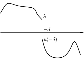
Figure 7. The geometry involved in the proof of Theorem 1.2: detachment from the boundary.

Consequently, to apply Lemma 3.1, it remains to check condition (3.2). For this, suppose by contradiction that $u(-d)=\min_{[-d,0]}u$. This, together with the assumptions on $u$ in (1.11) and (1.12), and recalling also (3.26), gives that

(3.29) $$\lambda:=\lim_{x\nearrow-d}u(x)\geqslant 0>u(p_{\star})\geqslant\min_{[-d,0]}u=u(-d),$$

see Figure 7.

Hence, by [MR4104542, Corollary 1.3(ii)] (see also [MR3532394] for related results), we infer that there exist $\mu>0$ and a continuous function $v$ in $\big{(}u(-d)-\mu,u(-d)+\mu\big{)}$ such that $v$ is the inverse function of $u$ (in the above domain of definition, with the understanding that $v=-d$ along the jump discontinuity of $u$ detected in (3.29)).

Now we pick a sequence of points $q_{k}\in(-d,0)$ with $q_{k}\searrow-d$ as $k\to+\infty$; in particular, we can assume that $u(q_{k})\in\big{(}u(-d)-\mu,u(-d)+\mu\big{)}$ and we thus obtain that $v(u(q_{k}))=q_{k}$. We have that

(3.30) $$u(q_{k})<u(-d),$$

otherwise, since $v(y)=-d$ for all $y\in\big{[}u(-d),\min\{\lambda,u(-d)+\mu\}\big{]}$, we would have that $-d=v(u(q_{k}))=q_{k}>-d$, which is a contradiction.

Having proved (3.30), we find that

$$u(q_{k})<u(-d)=u(p)=\min_{[-d,0]}u\leqslant u(q_{k})$$

and this is a contradiction that shows the validity of (3.2).

We can thereby apply Lemma 3.1 to complete the proof of Theorem 1.2.∎

4. Some comments about antisymmetric functions

Maximum principles in the presence of an odd symmetry have been already treated in the field of integro-differential equations (see for instance [MR3453602, MR4030266, MR4108219, MR4308250, JACK]). The main idea in this setting is that the operator can be rewritten as a different integro-differential operator acting only on functions defined in the halfspace, but still with a positive kernel (under certain assumptions on the original operator). For instance, the fractional Laplacian in $\mathbb{R}$ acting on odd functions $u$ can be rewritten as an operator $L_{s}u+cu$, where $c$ is a nonnegative function and $L_{s}$ is an integro-differential operator of the form

(4.1) $$L_{s}u(x)=\int_{0}^{+\infty}\big{(}u(x)-u(y)\big{)}K_{s}(x,y)\,dy$$

defined for all $x>0$, being $K_{s}(x,y)$ a nonnegative kernel. Thus, exploiting this observation, the usual proof for the maximum principle in $\mathbb{R}$ carries through also for this operator.

A natural question is whether or not a trick of this type, exploiting the antisymmetry of the functions, can work in this setting for antisymmetric nonlocal minimal graphs.

In a sense, the answer to this question is not completely clear: on the one hand, there are ways to rewrite the nonlocal mean curvature operator in the odd symmetric setting, but either the kernel obtained has not necessarily the right sign, or the structure of the operator is not immediately apt for a straightforward proof of the maximum principle.

In our opinion, the difference between the fractional Laplace framework and that of nonlocal minimal surfaces with respect to this point may be not merely algebraic in nature and instead reveals an interesting phenomenon due to the nonlinear and geometric structures of the problem (thus requiring a somewhat careful detection of the appropriate isometric regions in Section 3).

Let us explicitly point out some of the natural computations that one can perform to encode odd symmetry properties into the nonlocal mean curvature operator. First of all, at the level of a set $E$, the antisymmetric property considered in this paper reads that $X\in E$ if and only if $-X\in\mathbb{R}^{2}\setminus E$. Accordingly,

$$\chi_{\mathbb{R}^{2}\setminus E}(-X)-\chi_{E}(-X)=-\big{(}\chi_{\mathbb{R}^{2}\setminus E}(X)-\chi_{E}(X)\big{)},$$

leading to

$$\int_{\mathbb{R}^{2}}\frac{\chi_{\mathbb{R}^{2}\setminus E}(X)-\chi_{E}(X)}{|X-P|^{2+s}}\,dX$$

$$= \int_{(0,+\infty)\times\mathbb{R}}\frac{\chi_{\mathbb{R}^{2}\setminus E}(X)-\chi_{E}(X)}{|X-P|^{2+s}}\,dX+\int_{(-\infty,0)\times\mathbb{R}}\frac{\chi_{\mathbb{R}^{2}\setminus E}(X)-\chi_{E}(X)}{|X-P|^{2+s}}\,dX$$

$$= \int_{(0,+\infty)\times\mathbb{R}}\frac{\chi_{\mathbb{R}^{2}\setminus E}(X)-\chi_{E}(X)}{|X-P|^{2+s}}\,dX+\int_{(0,+\infty)\times\mathbb{R}}\frac{\chi_{\mathbb{R}^{2}\setminus E}(-X)-\chi_{E}(-X)}{|X+P|^{2+s}}\,dX$$

$$= \int_{(0,+\infty)\times\mathbb{R}}\frac{\chi_{\mathbb{R}^{2}\setminus E}(X)-\chi_{E}(X)}{|X-P|^{2+s}}\,dX-\int_{(0,+\infty)\times\mathbb{R}}\frac{\chi_{\mathbb{R}^{2}\setminus E}(X)-\chi_{E}(X)}{|X+P|^{2+s}}\,dX$$

$$= \int_{(0,+\infty)\times\mathbb{R}}\big{(}\chi_{\mathbb{R}^{2}\setminus E}(X)-\chi_{E}(X)\big{)}\,K(X,P)\,dX,$$

where

$$K(X,P):=\frac{1}{|X-P|^{2+s}}-\frac{1}{|X+P|^{2+s}}.$$

While this calculation reduces the nonlocal mean curvature to an integral in the halfplane, the kernel $K$ is not necessarily positive, for instance, if $P=(1,1)$ and $X=(1,-2)$, we have that

$$K(X,P)=\frac{1}{3^{2+s}}-\frac{1}{5^{\frac{2+s}{2}}}<0,$$

see Figure 8.

Figure 8. Difficulties arising in a straightforward proof of the antisymmetric maximum principle.

Another possible approach towards the rewriting of the nonlocal mean curvature operator consists in focusing on sets possessing a graph structure (say, in the plane, for simplicity). In this case, by equation (49) in [MR3331523], there exists a bounded, smooth, globally Lipschitz, strictly increasing and odd function $F$ such that, up to a real multiplicative constant, the nonlocal mean curvature at $(x,u(x))$ becomes

$$\int_{\mathbb{R}}F\left(\frac{u(x)-u(x+w)}{|w|}\right)\,\frac{dw}{|w|^{1+s}}=\int_{\mathbb{R}}F\left(\frac{u(x)-u(y)}{|x-y|}\right)\,\frac{dy}{|x-y|^{1+s}}.$$

Thus, if $u$ is odd symmetric, we obtain

$$\int_{0}^{+\infty}F\left(\frac{u(x)-u(y)}{|x-y|}\right)\,\frac{dy}{|x-y|^{1+s}}+\int_{0}^{+\infty}F\left(\frac{u(x)-u(-y)}{|x+y|}\right)\,\frac{dy}{|x+y|^{1+s}}$$

$$= \int_{0}^{+\infty}F\left(\frac{u(x)-u(y)}{|x-y|}\right)\,\frac{dy}{|x-y|^{1+s}}-\int_{0}^{+\infty}F\left(\frac{u(x)-u(y)-2u(x)}{|x+y|}\right)\,\frac{dy}{|x+y|^{1+s}},$$

which, due to the nonlinearity $F$, does not immediately lead to a nice equation as in (4.1).

Yet, one could try to modify this argument by using Lagrange’s Mean Value Theorem: in this way, we can write the nonlocal mean curvature operator as

$$\int_{0}^{+\infty}F\left(\frac{u(x)-u(x+w)}{|w|}\right)\,\frac{dw}{|w|^{1+s}}+\int_{0}^{+\infty}F\left(\frac{u(x)-u(x-w)}{|w|}\right)\,\frac{dw}{|w|^{1+s}}$$

$$= \int_{0}^{+\infty}F\left(\frac{u(x)-u(x+w)}{|w|}\right)\,\frac{dw}{|w|^{1+s}}-\int_{0}^{+\infty}F\left(\frac{u(x-w)-u(x)}{|w|}\right)\,\frac{dw}{|w|^{1+s}}$$

$$= \int_{0}^{+\infty}\frac{F^{\prime}(\xi_{u}(x,w))}{|w|^{2+s}}\,\Big{(}2u(x)-u(x+w)-u(x-w)\Big{)}\,dw,$$

even without the odd symmetry of $u$. In this case, the kernel $\frac{F^{\prime}(\xi_{u}(x,w))}{|w|^{2+s}}$ is positive, since $F$ is strictly increasing, and bounded from above by the kernel of the fractional Laplacian, since $F$ is globally Lipschitz.

Nonetheless, if $u$ is odd symmetric and, say, negative in $(2,+\infty)$ and presents a positive maximum in $[0,2]$, it is not necessarily true that $2u(x)-u(x+w)-u(x-w)\geqslant 0$. As an example, one can consider an odd function as above such that $u(1)=1$, $u(3)=-4$ and $u(4)=-2$: in this way, if $x:=1$ and $w:=4$, it follows that $2u(x)-u(x+w)-u(x-w)=2u(1)-u(5)-u(-3)=2+1-4<0$, see Figure 8.

For these reasons, it is not clear to us that a straightforward symmetric trick may lead to an antisymmetric maximum principle as in Theorem 1.2 without taking advantage of the cancellations provided by the isometric regions detected in Section 3.

In any case, we think that a proof of the antisymmetric maximum principle based solely on the detection of isometric regions, as presented in Section 3, is interesting in itself, since it explicitly identifies the convenient cancellations for such a result to hold.