Composition of the inclusive semi-leptonic decay of $B$ meson

Abstract

Utilizing the approach recently proposed for the inclusive semi-leptonic decay rate on the lattice, we compute the differential decay rate of a $B_{s}$ meson for various kinematical channels. The results are compared with the contributions from the ground states ($D$ and $D^{*}$) as well as from the orbitally excited states ($D^{**}$’s). The computation so far is carried out with an unphysically light bottom quark and strange spectator quark.

KEK-CP-0386

1 Introduction

Semi-leptonic decays of $B$ meson have been measured in various specific final states, such as $D^{(*)}\ell\nu$ or $D^{**}\ell\nu$. They can be used to determine the Cabibbo-Kobayashi-Maskawa (CKM) matrix element $|V_{cb}|$. (Here, we focus on the $b\to c$ decays, but the formulation and calculation method are applicable also for the $b\to u$ channels.) On the other hand, the experimentalists can also perform the so-called inclusive analysis, i.e. all possible final states including a charm quark are counted. Theoretically, such experimental results may be compared with the OPE analysis [1, 2] to determine $|V_{cb}|$.

More recently, one of the authors proposed a method to compute the inclusive decay rate using lattice QCD [3]. It utilizes a method to implicitly sum over all possible states to appear in two operator insertions on the lattice [4, 5]. To be explicit, we consider the forward-Compton amplitude of the form

$$\langle B(\bm{0})|\tilde{J}_{\mu}^{\dagger}(-\bm{q};t)\;\;\Big{|}\;\;\tilde{J}_{\nu}(\bm{q};0)|B(\bm{0})\rangle,$$ (1)

where two flavor-changing currents $J_{\mu}$ are inserted with a specific spatial momentum $\bm{q}$. The vertical line in the middle represents all possible states of the specified quantum number that can contribute. The key idea is to use the time separation $t$ to control the weight among the states having different energies. The method allows a fully non-perturbative computation of the inclusive decay rate, so that one can verify the OPE-based calculation that has been used so far.

There is a long-standing tension between the $|V_{cb}|$ determinations from the exclusive and inclusive channels. The aim of our study is to understand the cause of the problem by providing a framework of theoretical calculation that can be applied for both analyses. We may also identify the contribution from the excited state $D$ mesons and $D\pi$ continuum states from the lattice data, which would enable another test of the calculation by comparing with the corresponding experimental data.

This contribution mainly describes the lattice computatin, and the comparison with the OPE calculation for the same set of parameters is separately presented in [6].

2 Inclusive decay rate: outline of the formalism

Here we outline the method proposed in [3].

The differential decay rate of the $B$ meson can be decomposed as $d\Gamma\sim|V_{cb}|^{2}l^{\mu\nu}W_{\mu\nu}dq_{0}d\bm{q}$, where the leptonic tensor $l^{\mu\nu}$ is determined by the kinematics of the final state leptons $\ell$ and $\nu$. The momentum transfer to the lepton pair is $q=(q_{0},\bm{q})$. The hadronic tensor $W_{\mu\nu}$, on the other hand, has a complicated structure

$$W_{\mu\nu}(q_{0},\bm{q})\sim\sum_{X}(2\pi)^{3}\delta^{(4)}(p_{B}-q-p_{X})\frac{1}{2m_{B}}\langle B(\bm{p}_{B})|J_{\mu}^{\dagger}(0)|X\rangle\langle X|J_{\nu}(0)|B(\bm{p}_{B})\rangle,$$ (2)

where the flavor-changing current $J_{\mu}$ induces the decay $b\to c$, and the sum of the state $X$ runs over all possible final states including a charm quark. When the initial $B$ meson is at rest, $\bm{p}_{B}=\bm{0}$, the final hadronic state $X$ has a momentum $\bm{p}_{X}=-\bm{q}$ given by the momentum transfer $q$. Since it depends on the structure of the initial $B$ meson state, the hadronic tensor $W_{\mu\nu}$ is also called the structure function.

We notice that the sum over the states $X$ may be considered as an integral over its energy $p_{X}^{0}$. Because of the $\delta$-function, it is given by $p_{X}^{0}\equiv\omega=m_{B}-q_{0}$. Thus, the structure function picks up the state of energy $\omega$, and

$$W_{\mu\nu}(\omega,\bm{q})\sim\langle B(\bm{0})|\tilde{J}_{\mu}^{\dagger}(-\bm{q})\delta(\omega-\hat{H})\tilde{J}_{\nu}(\bm{q})|B(\bm{0})\rangle.$$ (3)

Here $\tilde{J}_{\mu}(\bm{q})$ is a Fourier-transform of the current. We specify the energy $\omega$ by inserting the $\delta$-function $\delta(\omega-\hat{H})$ between the currents. ($\hat{H}$ is the Hamiltonian of QCD.)

The total decay rate can then be written as

$$\Gamma\propto|V_{cb}|^{2}\int_{0}^{\bm{q}^{2}_{\mathrm{max}}}d\bm{q}^{2}\int_{\sqrt{m_{D}^{2}+\bm{q}^{2}}}^{m_{B}-\sqrt{\bm{q}^{2}}}d\omega\,K(\omega;\bm{q}^{2})\langle B(\bm{0})|\tilde{J}_{\mu}^{\dagger}(-\bm{q})\delta(\omega-\hat{H})\tilde{J}_{\nu}(\bm{q})|B(\bm{0})\rangle,$$ (4)

where $K(\omega;\bm{q}^{2})$ is a kinematical factor originating from the leptonic tensor.

The problem is then how to compute the integral over the final-state energy $\omega$ with the weight of $K(\omega;\bm{q})$. The upper limit of the $\omega$-integral is also imposed by the kinematics; we may include them in $K(\omega,\bm{q}^{2})$ using the Heaviside function as $\theta(m_{B}-\sqrt{\bm{q}^{2}}-\omega)$ while extending the upper limit to infinity. Then, we can rewrite the $\omega$-integral using

$$\int_{0}^{\infty}\!d\omega\,K(\omega;\bm{q}^{2})\langle B(\bm{0})|\tilde{J}_{\mu}^{\dagger}(-\bm{q})\delta(\omega-\hat{H})\tilde{J}_{\nu}(\bm{q})|B(\bm{0})\rangle=\langle B(\bm{0})|\tilde{J}_{\mu}^{\dagger}(-\bm{q})K(\hat{H};\bm{q}^{2})\tilde{J}_{\nu}(\bm{q})|B(\bm{0})\rangle.$$ (5)

Here, the kinematical factor is promoted to an operator by replacing $\omega$ by $\hat{H}$. On the other hand, what one can calculate on the lattice is the Compton amplitude (1), which is also written in the form

$$\langle B(\bm{0})|\tilde{J}_{\mu}^{\dagger}(-\bm{q};t)\tilde{J}_{\nu}(\bm{q};0)|B(\bm{0})\rangle=\langle B(\bm{0})|\tilde{J}_{\mu}^{\dagger}(-\bm{q};t)e^{-\hat{H}t}\tilde{J}_{\nu}(\bm{q};0)|B(\bm{0})\rangle,$$ (6)

because the time separation between the currents may be described by the transfer matrix $\exp(-\hat{H}t)$.

Given the similarity between (5) and (6), one notices that (5) can be evaluated if the kernel operator $K(\hat{H})$ can be approximated in the form $K(\hat{H})\simeq k_{0}+k_{1}e^{-\hat{H}}+k_{2}e^{-2\hat{H}}+\cdots+k_{N}e^{-N\hat{H}}$ with some coefficients $k_{j}$. Such approximation can be constructed using the Chebyshev polynomials:

$$K(\omega)\simeq\frac{c_{0}}{2}+\sum_{j=1}^{N}c_{j}^{*}T_{j}^{*}(e^{-\omega}),$$ (7)

where $T_{j}^{*}(x)$’s are shifted Chebyshev polynomials defined as $T_{j}^{*}(x)=T_{j}(2x-1)$ from the standard Chebyshev polynomial $T_{j}(z)$. Thus, the shifted Chebyshev polynomials are defined for $0\leq x\leq 1$ or $\infty\geq\omega\geq 1$ since $x=e^{-\omega}$. The coefficients $c_{j}^{*}$ can be easily computed for arbitrary kernel operator $K(\omega)$. Since the Chebyshev polynomials $T_{j}^{*}(e^{-\omega})$ are constructed from polynomials $(e^{-\omega})^{m}$ with positive integer $m$’s, they are related to the transfer matrix $e^{-\hat{H}t}$ appearing in (6). The forward Compton amplitude (6) can therefore be used to approximate the target quantity (5).

The kernel function $K(\omega;\bm{q}^{2})$ has the following structure

$$K(\omega;\bm{q}^{2})\sim e^{2\omega t_{0}}(m_{B}-\omega)^{l}\theta(m_{B}-\sqrt{\bm{q}^{2}}-\omega).$$ (8)

Here, $(m_{B}-\omega)^{l}$ ($l=$ 0, 1 or 2) originates from the leptonic tensor; the factor $e^{2\omega t_{0}}$ is introduced to avoid any divergence due to a contact term between the two currents by normalizing the matrix element by the value at a small time separation $t_{0}$. The Heaviside $\theta$-function $\theta(m_{B}-\sqrt{\bm{q}^{2}}-\omega)$ implements the upper limit of the $\omega$ integral (see (4)).

The Chebyshev approximation of the kernel function is harder when the function contains a discontinuous (or even rapid) change such as that given by the $\theta$-function, and we introduce a smearing to modify the $\theta$-function to a smooth function with a smearing width $\sigma$. (To be explicit we use the sigmoid function, but the details are not important.) We need to take the limit $\sigma\to 0$ to obtain the final result.

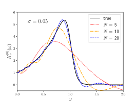
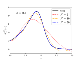
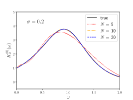
Figure 1: Kernel function for $l=0$ with smearing with the width $\sigma=0.05$ (left panel) 0.1 (middle) and 0.2 (right). Together with the true function (thich curve), Chebyshev approximations of order $N$ = 5, 10 and 20 are shown (dashed and dotted curves). The threshold is at $\omega\simeq$ 1.0. (All in the lattice unit.)

The kernel function $K(\omega)$ is plotted for $l=0$ with the smearing width $\sigma$ = 0.05, 0.1 and 0.2 in Fig. 1. Around the threshold of the $\theta$-function, the shape is smeared so that the function is smoothed. The Chebyshev approximations are also shown in the plots for the order of polynomial $N$ = 5, 10 and 20. The approximation is rather precise when the width is large ($\sigma$ = 0.2 on the right panel) even with the limited order of polynomials, while it gets harder for small $\sigma$. Although it would depend on the precision one wants to achieve, it seems that at least $N$ = 20 is necessary to achieve a sensible approximation for $\sigma$ = 0.05.

3 Compton amplitude

We compute the Compton amplitude of the form (6) on the lattice. It is obtained from a four-point function with two flavor-changing $V-A$ currents inserted with time separation $t$ between interpolating operators to create or annihilate the $B$ meson. To compute the amplitude with all possible combinations of spin orientations $\mu$ and $\nu$ we have to repeat the computation of sequential sources many times, as well as for the choices of final momenta. (The initial $B$ meson is set at rest.)

The computation is done on a lattice of $48^{3}\times 96$ at $1/a\simeq$ 3.6 GeV generated including up, down and strange sea quarks described by the Mobius domain-wall fermions. The ensemble is the same as that used in [3] and is a part of the large set of ensembles generated and used in [7]. The valence quarks are also domain-wall fermions; the charm quark mass is tuned to its physical value while the bottom quark mass is taken (unphysically) light and about 2.7 GeV. The spectator quark is strange in this study, so that the initial state is (unphysically light) $B_{s}$ meson.

The statistics is 100 gauge configurations and the measurement is repeated four times on each configuration with different source time slices.

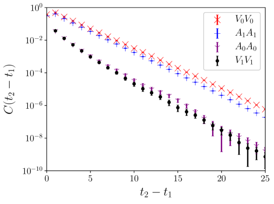
Figure 2: Compton amplitude as a function of the time separation. The final state has a vanishing spatial momentum. Different current insertions are shown together: vector ($V$) and axial-vector ($A$) currents in the temporal ($0$) and spatial ($k=1$) directions.

Fig. 2 shows the Compton amplitude (6) as a function of the time separation $t\equiv t_{2}-t_{1}$ for the case of zero spatial momentum in the final state. The current insertions are either $V(t_{2})V(t_{1})$ or $A(t_{2})A(t_{1})$ combinations of vector ($V$) or axial-vector ($A$) currents. Non-zero values are obtained for $(\mu,\nu)=(0,0)$ (temporal) or $(\mu,\nu)=(k,k)$ (spatial) orientations of the currents. Among them, the $V_{0}V_{0}$ and $A_{k}A_{k}$ combinations show the largest signal due to the $S$-wave ground-state contributions from the pseudo-scalar $D_{s}$ ($0^{-}$) or vector $D_{s}^{*}$ ($1^{-}$) meson. If we look into the details, the amplitude of $V_{0}V_{0}$ is slightly larger than $A_{k}A_{k}$ because the pseudo-scalar state is lighter.

The other channels $A_{0}A_{0}$ and $V_{k}V_{k}$ show substantially ($\times 50$) smaller contributions. They correspond to the scalar ($0^{+}$) and axial-vector ($1^{+}$) states, respectively. In the quark model, they are $P$-wave states and their coupling to the initial $B_{s}$ meson is weak. According to the analysis based on the heavy quark effective theory (HQET) [8], the $B\to D^{**}\ell\nu$ ($D^{**}$ denotes the $P$-wave states generically) form factor is suppressed as $\bar{\Lambda}/2m_{c}$ with $\bar{\Lambda}$ a typical QCD scale $\sim$ 300 MeV compared to the $B\to D^{(*)}\ell\nu$ form factors, which is $O(1)$, so that the Compton amplitude is suppressed by $(\bar{\Lambda}/2m_{c})^{2}\sim$ 0.01.

These opposite parity channels can also couple to $DK$ continuum, which is heavier than the above mentioned $P$-wave mesons. Interestingly, the data show the contributions of such excited states at small time separations $t_{2}-t_{1}\lesssim$ 5.

4 Inclusive decay rate

According to (4), we obtain the total decay rate from the Compton amplitudes as described in the previous section. The kinematical factor $K(\omega;\bm{q}^{2})$ is promoted to the integral kernel for the $\omega$-integral. The spatial momentum integration over $\bm{q}^{2}$ is yet to be performed.

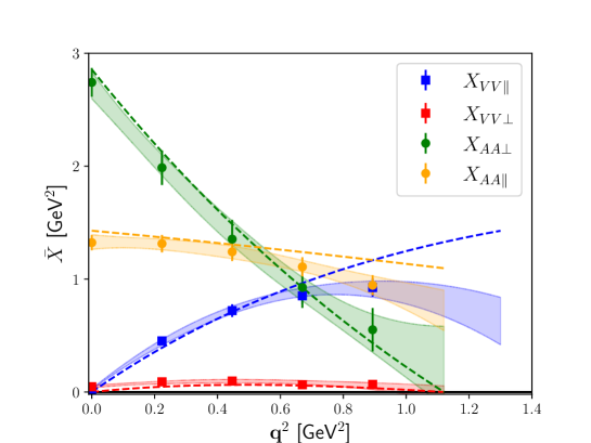
Figure 3: Differential decay rate divided by $|\bm{q}|$ as a function of $\bm{q}^{2}$. The results are shown for four different channels: $VV_{\parallel}$, $VV_{\perp}$, $AA_{\parallel}$ and $AA_{\perp}$. (For more details, see the text.) The bands are contributions of ground state, $D$ or $D^{*}$ meson, as estimated using the corresponding form factors.

The results for the differential decay rate (divided by $|\bm{q}|$) are plotted in Fig. 3 as a function of $\bm{q}^{2}$. Four contributions are plotted separately: $VV$ and $AA$ denote the two currents inserted, which are decomposed from the $V-A$ weak currents. The other possible combinations, $VA$ and $AV$, do not contribute for the differential decay rate after integrating over the lepton energy $E_{\ell}$. The current orientations, $\parallel$ and $\perp$, distinguish the currents in the direction parallel or perpendicular to the momentum $\bm{q}$. For instance, when the momentum $\bm{q}$ is in the $z$-direction, $(0,0,1)$, the $VV\!\perp$ represent the contribution from $V^{1}V^{1}$ and $V^{2}V^{2}$, while $VV\!\parallel$ is that of $V^{3}V^{3}$, $V^{3}V^{0}$, $V^{0}V^{3}$ and $V^{0}V^{0}$.

Also shown by the bands are the corresponding contributions from the ground states, i.e. from $B_{s}\to D_{s}\ell\nu$ for $VV\!\parallel$ and from $B_{s}\to D_{s}^{*}\ell\nu$ for others. We have separately computed the form factors of these decay modes, $h_{+}(w)$, $h_{-}(w)$ and $h_{A_{1}}(w)$, $h_{A_{2}}(w)$, $h_{A_{3}}(w)$, $h_{V}(w)$. (The computation is done along with [9], and the analysis method is essentially the same.) Using these results, the differential decay rate for each channel can be constructed.

As one can see, the inclusive decay rate is dominated by the ground state contributions for each channel. This is not unreasonable because the initial state is lighter than the physical $B_{s}$ meson. Kinematically there is not so much room to produce extra particles other than $D_{s}^{(*)}$. Also, the heavy quark symmetry implies that the wave function of light degrees of freedom are very similar between the initial $B_{s}$ and final $D_{s}^{(*)}$ states, so that the overlap between these states are enhanced when the initial and final quark masses are similar, especially near the zero-recoil ($\bm{q}\sim 0$) limit.

As we mentioned in the previous section, the contribution from the excited states including those from the $P$-wave meson is visible in the Compton amplitudes. It is however not significant for the differential decay rate, since their contributions are roughly 50 times smaller.

5 Summary

Framework to compute inclusive decay rate on the lattice is now available. The essential step is the reconstruction of the energy integral from Euclidean lattice correlators corresponding to the Compton amplitudes. In our case, it is implemented using the Chebyshev approximation. Other methods, such as the Backus-Gilbert method can also do the job [10, 11]. The method to compute the energy integral can be also applied for calculations of (not so) deep inelastic scattering cross section, $\sigma(\ell N\to\ell^{\prime}X)$ [12] as well as those of spectral sum of hadronic vacuum polarization [13].

The Compton amplitudes contain the contributions from ground states and excited states. With the lattice parameters taken in this work the ground state contributions dominate the differential cross section, although the excited state contributions such as those from the $P$-wave states are visible in the Compton amplitude.

The present results can already been used to compare with the analytic OPE calculations. Even though the $b$-quark mass is not tuned to the physical value, the comparison would still yield useful tests of the theoretical approaches [6].

References

- [1] B. Blok, L. Koyrakh, M. A. Shifman and A. I. Vainshtein, Phys. Rev. D 49, 3356 (1994) [erratum: Phys. Rev. D 50, 3572 (1994)] doi:10.1103/PhysRevD.50.3572 [arXiv:hep-ph/9307247 [hep-ph]].
- [2] A. V. Manohar and M. B. Wise, Phys. Rev. D 49, 1310-1329 (1994) doi:10.1103/PhysRevD.49.1310 [arXiv:hep-ph/9308246 [hep-ph]].
- [3] P. Gambino and S. Hashimoto, Phys. Rev. Lett. 125, no.3, 032001 (2020) doi:10.1103/PhysRevLett.125.032001 [arXiv:2005.13730 [hep-lat]].
- [4] S. Hashimoto, PTEP 2017, no.5, 053B03 (2017) doi:10.1093/ptep/ptx052 [arXiv:1703.01881 [hep-lat]].
- [5] G. Bailas, S. Hashimoto and T. Ishikawa, PTEP 2020, no.4, 043B07 (2020) doi:10.1093/ptep/ptaa044 [arXiv:2001.11779 [hep-lat]].
- [6] P. Gambino, S. Hashimoto and S. Mächler, [arXiv:2111.02833 [hep-ph]]; PoS(LATTICE2021)512.
- [7] K. Nakayama, B. Fahy and S. Hashimoto, Phys. Rev. D 94, no.5, 054507 (2016) doi:10.1103/PhysRevD.94.054507 [arXiv:1606.01002 [hep-lat]].
- [8] A. K. Leibovich, Z. Ligeti, I. W. Stewart and M. B. Wise, Phys. Rev. D 57, 308-330 (1998) doi:10.1103/PhysRevD.57.308 [arXiv:hep-ph/9705467 [hep-ph]].
- [9] T. Kaneko et al., PoS(LATTICE2021)561.
- [10] M. T. Hansen, H. B. Meyer and D. Robaina, Phys. Rev. D 96, no.9, 094513 (2017) doi:10.1103/PhysRevD.96.094513 [arXiv:1704.08993 [hep-lat]].
- [11] M. Hansen, A. Lupo and N. Tantalo, Phys. Rev. D 99, no.9, 094508 (2019) doi:10.1103/PhysRevD.99.094508 [arXiv:1903.06476 [hep-lat]].
- [12] H. Fukaya, S. Hashimoto, T. Kaneko and H. Ohki, Phys. Rev. D 102, no.11, 114516 (2020) doi:10.1103/PhysRevD.102.114516 [arXiv:2010.01253 [hep-lat]].
- [13] T. Ishikawa and S. Hashimoto, Phys. Rev. D 104, no.7, 074521 (2021) doi:10.1103/PhysRevD.104.074521 [arXiv:2103.06539 [hep-lat]].