Cubic regularization methods with second-order complexity guarantee based on a new subproblem reformulation

Abstract

The cubic regularization (CR) algorithm has attracted a lot of attentions in the literature in recent years. We propose a new reformulation of the cubic regularization subproblem. The reformulation is an unconstrained convex problem that requires computing the minimum eigenvalue of the Hessian. Then based on this reformulation, we derive a variant of the (non-adaptive) CR provided a known Lipschitz constant for the Hessian and a variant of adaptive regularization with cubics (ARC). We show that the iteration complexity of our variants matches the best known bounds for unconstrained minimization algorithms using first- and second-order information. Moreover, we show that the operation complexity of both of our variants also matches the state-of-the-art bounds in the literature. Numerical experiments on test problems from CUTEst collection show that the ARC based on our new subproblem reformulation is comparable to existing algorithms.

1 Introduction

Consider the generic unconstrained optimization problem

$$\min_{x\in\mathbb{R}^{n}}f(x),$$ (1)

where $f:{\mathbb{R}}^{n}\rightarrow{\mathbb{R}}$ is a twice Lipschitz continuously differentiable and possibly nonconvex function. Recently, the cubic regularization (CR) algorithm nesterov2006cubic ; cartis2011adaptive or its variants has attracted a lot of attentions for solving problem (1), due to its practical efficiency and elegant theoretical convergence guarantees. Each iteration of the CR solves the following subproblem

$$\min_{s\in\mathbb{R}^{n}}m(s):=\frac{1}{2}s^{\top}Hs+g^{\top}s+\frac{\sigma}{3}\left\lVert s\right\rVert^{3},$$ (CRS)

where $H$ and $g$ represent the Hessian and gradient of the function $f$ at the current iterate, respectively, $\left\lVert\cdot\right\rVert$ denotes the Euclidean $l_{2}$ norm, $H$ is an $n\times n$ symmetric matrix (possibly non-positive semidefinite) and $\sigma$ is a regularization parameter that may be adaptive during the iterations. This model can be seen as a second-order Taylor expansion plus a cubic regularizer that makes the next iterate not too far away from the current iterate. It is well known that under mild conditions (nesterov2006cubic ; cartis2011adaptive ), the CR converges to a point satisfying the second-order necessary condition (SONC), i.e.,

$$\nabla f(x)=0,\quad\nabla^{2}f(x)\succeq 0,$$

where $(\cdot)\succeq 0$ means $(\cdot)$ is a positive semidefinite matrix. In the literature, it is of great interests to find a weaker condition than SONC, i.e.,

$$\|\nabla f(x)\|<\epsilon_{g},\quad\lambda_{\min}(\nabla^{2}f(x))\geq-\epsilon_{H},\quad\epsilon_{g},\epsilon_{H}>0,$$ (2)

where $\lambda_{\min}(H)$ denotes the minimum eigenvalue for a matrix $H$. Condition (2) is often said to be $(\epsilon_{g},\epsilon_{H})$ stationary.

The CR algorithm was first considered by Griewank in an unpublished technical report (griewank1981modification ). Nesterov and Polyak nesterov2006cubic proposed the CR in a different perspective and demonstrated that it takes ${\mathcal{O}}(\epsilon_{g}^{-3/2})$ iterations to find an $(\epsilon_{g},\epsilon_{g}^{1/2})$ stationary point if each subproblem is solved exactly. As in general the Lipschitz constant of the Hessian is difficult to estimate, Cartis et al. cartis2011adaptive ; cartis2011adaptive2 proposed an adaptive version of the CR algorithm, called the ARC (adaptive regularization with cubics), and showed that it admits an iteration complexity bound ${\mathcal{O}}\left(\max\{\epsilon_{g}^{-3/2},\epsilon_{H}^{-3}\}\right)$ to find an $(\epsilon_{g},\epsilon_{H})$ stationary point, when the subproblems are solved inexactly and the regularization parameter $\sigma>0$ is chosen adaptively.

Besides iteration complexity ${\mathcal{O}}(\epsilon_{g}^{-3/2})$, many subsequent studies proposed variants of the CR or other second-order methods that also have an operation complexity ${\mathcal{\tilde{O}}}({\epsilon_{g}^{-7/4}})$ (where ${\mathcal{\tilde{O}}}(\cdot)$ hides the logarithm factors), with high probability, for finding an $(\epsilon_{g},\epsilon_{g}^{1/2})$ stationary point of problem (1). Here, a unit operation can be a function evaluation, gradient evaluation, Hessian evaluation or a matrix vector product (curtis2021trust ). Based on the CR algorithm, Agarwal et al. agarwal2017finding derived an algorithm with such an operation complexity bound, where the heart of the algorithm is a subproblem solver that returns, with high probability, an approximate solution to the problem (CRS) in ${\mathcal{\tilde{O}}}(\epsilon_{g}^{-1/4})$ operations. After that, Carmon et al. carmon2018accelerated proposed an accelerated gradient method that also converges to an $(\epsilon_{g},\epsilon_{g}^{1/2})$ stationary point with an operation complexity ${\mathcal{\tilde{O}}}({\epsilon_{g}^{-7/4}})$. Royer and Wright royer2018complexity proposed a hybrid algorithm that combines Newton-like steps, the CG method for inexactly solving linear systems, and the Lanczos procedure for approximately computing negative curvature directions, which was shown to have an operation complexity ${\mathcal{\tilde{O}}}({\epsilon_{g}^{-7/4}})$ to achieve an $(\epsilon_{g},\epsilon_{g}^{1/2})$ stationary point. Royer et al. royer2020newton proposed a variant of Newton-CG algorithm with the same complexity guarantee. Very recently, Curtis et al. curtis2021trust considered a variant of trust-region Newton methods based on inexactly solving the trust region subproblem by the well known “trust-region Newton-conjugate gradient” method, whose complexity also matches the-state-of-the-art. All the above mentioned methods carmon2018accelerated ; royer2018complexity ; royer2020newton ; curtis2021trust converge with high probability like agarwal2017finding , which is due to the use of randomized iterative methods for approximately computing the minimum eigenvalue, e.g., the Lanczos procedure.

Despite theoretical guarantees, the practical efficiency of solving (CRS) heavily effects the convergence of the CR algorithm. Although it is one of the most successful algorithms for solving (CRS) in practice, the Krylov subspace method (cartis2011adaptive ) may fail to converge to the true solution of (CRS) in the hard case or close to being in the hard case. Carmon and Duchi carmon2018analysis provided the first convergence rate analysis of the Krylov subspace method in the easy case, based on which the authors further propose a CR algorithm with an operation complexity ${\mathcal{\tilde{O}}}({\epsilon_{g}^{-7/4}})$ in carmon2020first . Carmon and Duchi carmon2019gradient also showed the gradient descent method that works in both the easy and hard cases is able to converge to the global minimizer if the step size is sufficiently small, though the convergence rate is worse than the Krylov subspace method. Based on a novel convex reformulation of (CRS), Jiang et al. jiang2021accelerated proposed an accelerated first-order algorithm that works efficiently in practice in both the easy and hard cases, and meanwhile enjoys theoretical guarantees of the same order with the Krylov subspace method.

However, the methods in the literature (royer2018complexity ; carmon2018accelerated ; royer2020newton ; nesterov2006cubic ; cartis2011adaptive ; cartis2011adaptive2 ; agarwal2017finding ; carmon2020first ; jiang2021accelerated ), either somehow deviate the framework of the CR or ARC algorithms, and/or do not present good practical performance and an ${\mathcal{\tilde{O}}}({\epsilon_{g}^{-7/4}})$ operation complexity simultaneously. Our goal in this paper is to propose variants of the CR and ARC based on new subproblem reformulations that achieve the state-of-the-art complexity bounds and also remain close to the practically efficient CR and ARC algorithms. Motivated by the reformulation in jiang2021accelerated , we deduce a new unconstrained convex reformulation for (CRS). Our reformulation explores hidden convexity of (CRS), where similar ideas also appear in the (generalized) trust region subproblem (flippo1996duality ; ho2017second ; wang2017linear ; jiang2019novel ). The main cost of the reformulation is computing the minimum eigenvalue of the Hessian. We propose a variant of the CR algorithm with strong complexity guarantee. We consider the more realistic case where eigenvalues of Hessians are computed inexactly. In this setting, we suppose the Lipschitz constant of the Hessian is given as $L$, the parameter $\sigma=L/2$ is non-adaptive, and each subproblem is also solved approximately. We prove that our algorithm converges to an $(\epsilon_{g},\sqrt{L\epsilon_{g}})$ stationary point with an iteration complexity ${\mathcal{O}}({\epsilon_{g}^{-3/2}})$. Moreover, we further show that each iteration costs ${\mathcal{\tilde{O}}}({\epsilon_{g}^{-1/4}})$ when the minimum eigenvalue of the Hessian is inexactly computed by the Lanczos procedure, and the subproblem, which is regularized to be strongly convex, is approximately solved by Nesterov’s accelerated gradient method (NAG) nesterov2018lectures in each iteration. Combining the above facts, we further demonstrate that our algorithm has an operation complexity ${\mathcal{\tilde{O}}}({\epsilon_{g}^{-7/4}})$ for finding an $(\epsilon_{g},\sqrt{L\epsilon_{g}})$ stationary point. Based on the reformulation, we also propose a variant of the ARC with similar iteration and operation complexity guarantees, where $\sigma_{k}$ is adaptive in each iteration.

The remaining of this paper is organized as follows. In Section 2, we derive our unconstrained convex reformulation for (CRS), describe the CR and ARC algorithms and the basic setting, and give unified convergence analysis for sufficient decrease of the model function in one iteration. In Sections 3 and 4, we give convergence analysis for the CR and ARC algorithms for finding an approximate second-order stationary point with both iteration complexity and operation complexity bounds that match the best known ones, respectively. In Section 5, we compare numerical performance of an ARC embedded by our reformulation with ARCs based on existing subproblem solvers. We conclude our paper in Section 6.

2 Preliminaries

The structure of this section is as follows. In Section 2.1, we first propose our reformulation for the subproblem (CRS). Then in Section 2.2, we mainly describe the framework of our variants of the CR and ARC algorithms and also state our convergence results. Finally in Section 2.3, we give unified convergence analysis of one iteration progress for both the CR and ARC algorithms.

2.1 A new convex reformulation for (CRS)

In this subsection, we introduce a new reformulation for (CRS) when $\lambda_{\min}(H)<0$, i.e., the minimum eigenvalue of $H$ is negative. First recall the reformulation proposed in jiang2021accelerated

$$\min_{s,y} ~{}g^{\top}s+\frac{1}{2}s^{\top}\left(H-\alpha I\right)s+\frac{\sigma}{3}y^{3/2}+\frac{\alpha}{2}y$$ (3)

$$\ \,\mathrm{s.t.} ~{}y\geq\|s\|^{2},\quad y\geq\frac{\alpha^{2}}{\sigma^{2}},$$

where $\alpha=\lambda_{\min}(H)$. However, this reformulation may be ill-conditioned and cause numerical instability when $y$ is small since the Hessian of the objective function for $y$ is $\frac{\sigma}{4}y^{-1/2}$, which approaches infinity when $y\rightarrow 0$. Unfortunately, this is the case for the CR or ARC algorithms when the iteration number $k$ becomes large. We also found that due to this issue and that $y$ is of the same order with $\|s\|^{2}$, CR or ARC based on solving subproblem (3) cannot achieve the state-of-the-art operation complexity ${\mathcal{\tilde{O}}}({\epsilon_{g}^{-7/4}})$ for finding an $(\epsilon_{g},\sqrt{L\epsilon_{g}})$ stationary point. To amend this issue, we proposed the following reformulation,

$$\min_{s,y} ~{}\hat{m}(s,y):=g^{\top}s+\frac{1}{2}s^{\top}\left(H-\alpha I\right)s+\frac{\sigma}{3}y^{3}+\frac{\alpha}{2}y^{2}$$ (CRS_r)

$$\ \,\mathrm{s.t.} ~{}y\geq\|s\|,\quad y\geq-\frac{\alpha}{\sigma},$$

so that $y$ is of the same order with $\|s\|$.

One key observation of this paper is that (CRS_r) can be simplified into a convex problem with single variable $s$, by applying partial minimization on $y$. Note that given any $s\in{\mathbb{R}}^{n}$, the $y$-problem of (CRS_r) is

$$\min_{y\in{\mathbb{R}}}\left\{\frac{\sigma}{3}y^{3}+\frac{\alpha}{2}y^{2}:\ y\geq\|s\|,\ y\geq-\frac{\alpha}{\sigma}\right\},$$

whose optimal solution is uniquely given by

$$y=\max\left\{\|s\|,-\frac{\alpha}{\sigma}\right\}.$$ (4)

This is because the derivative of the objective function is $\sigma y^{2}+\alpha y$, satisfying

$$\sigma y^{2}+\alpha y=\sigma y\left(y+\frac{\alpha}{\sigma}\right)\geq 0,$$

due to the constraints $y\geq 0$ and $y\geq-\frac{\alpha}{\sigma}$. Substituting (4) into (CRS_r), we obtain that (CRS_r) is equivalent to

$$\min_{s\in{\mathbb{R}}^{n}}\left\{\tilde{m}(s):=g^{\top}s+\frac{1}{2}s^{\top}(H-\alpha I)s+J_{\alpha,\sigma}(s)\right\},$$ (CRS_u)

where

$$J_{\alpha,\sigma}(s):=\frac{\sigma}{3}\left[\max\left\{\|s\|,-\frac{\alpha}{\sigma}\right\}\right]^{3}+\frac{\alpha}{2}\left[\max\left\{\|s\|,-\frac{\alpha}{\sigma}\right\}\right]^{2}.$$ (5)

In the following, we show that $J_{\alpha,\sigma}(s)$ is a convex and continuously differentiable function.

Proposition 1

For any $\sigma>0$ and $\alpha\in{\mathbb{R}}$, $J_{\alpha,\sigma}(s)$ is convex and continuously differentiable on ${\mathbb{R}}^{n}$. Moreover, we have

$$\nabla J_{\alpha,\sigma}(s)=\left[\sigma\|s\|+\alpha\right]_{+}\cdot s,\qquad\forall\,s\in{\mathbb{R}}^{n},$$

where $[a]_{+}=\max\{a,0\}$ for any $a\in{\mathbb{R}}$.

Proof

We consider the two cases (a) $\alpha\geq 0$ and (b) $\alpha<0$ separately.

• If $\alpha\geq 0$, then by $\sigma>0$, we have $\|s\|\geq-\alpha/\sigma$ for all $s\in{\mathbb{R}}^{n}$. Thus, $J_{\alpha,\sigma}(s)$ reduces to

  $$J_{\alpha,\sigma}(s)=\frac{\sigma}{3}\|s\|^{3}+\frac{\alpha}{2}\|s\|^{2},\quad\forall\,s\in{\mathbb{R}}^{n}.$$

  It is clear that in this case $J_{\alpha,\sigma}(s)$ is convex and continuously differentiable, and

  $$\nabla J_{\alpha,\sigma}(s)=\sigma\|s\|s+\alpha s=(\sigma\|s\|+\alpha)\cdot s=\left[\sigma\|s\|+\alpha\right]_{+}\cdot s,$$

  where the last equality is due to $\alpha\geq 0$.

• Now we consider the case $\alpha<0$. Note that the following identity holds for any $\sigma>0$, $\alpha,y\in{\mathbb{R}}$:

  $$\frac{\sigma}{3}y^{3}+\frac{\alpha}{2}y^{2}=\frac{\sigma}{3}\left(y+\frac{\alpha}{\sigma}\right)^{3}-\frac{\alpha}{2}\left(y+\frac{\alpha}{\sigma}\right)^{2}+\frac{\alpha^{3}}{6\sigma^{2}}.$$

  By this, we can rewrite $J_{\alpha,\sigma}(s)$ in (5) as

  $$J_{\alpha,\sigma}(s)=\frac{\sigma}{3}\left[\|s\|+\frac{\alpha}{\sigma}\right]_{+}^{3}-\frac{\alpha}{2}\left[\|s\|+\frac{\alpha}{\sigma}\right]_{+}^{2}+\frac{\alpha^{3}}{6\sigma^{2}}.$$ (6)

  Note that $\|s\|+\alpha/\sigma$ is a convex function of $s$. In addition, $[\cdot]_{+}^{3}$ and $[\cdot]_{+}^{2}$ are both non-decreasing convex functions. Thus, we obtain that

  $$h_{1}(s):=\left[\|s\|+\frac{\alpha}{\sigma}\right]_{+}^{3}\quad\mbox{and}\quad h_{2}(s):=\left[\|s\|+\frac{\alpha}{\sigma}\right]_{+}^{2}$$

  are convex functions. This, together with $\alpha<0$ and (6), implies that $J_{\alpha,\sigma}(s)$ is convex. Also, it is easy to verify that

  $$\nabla h_{1}(s) =\left\{\begin{aligned} &0,\qquad\qquad\qquad\qquad\ \mbox{if}\ \|s\|\leq-\frac{\alpha}{\sigma},\\ &3\left(\|s\|+\frac{\alpha}{\sigma}\right)^{2}\cdot\frac{s}{\|s\|},~{}~{}\mbox{if}\ \|s\|>-\frac{\alpha}{\sigma};\end{aligned}\right.$$

  $$\nabla h_{2}(s) =\left\{\begin{aligned} &0,\qquad\qquad\qquad\qquad\ \mbox{if}\ \|s\|\leq-\frac{\alpha}{\sigma},\\ &2\left(\|s\|+\frac{\alpha}{\sigma}\right)\cdot\frac{s}{\|s\|},\quad\mbox{if}\ \|s\|>-\frac{\alpha}{\sigma}.\end{aligned}\right.$$

  This, together with (6), implies that

  $$\nabla J_{\alpha,\sigma}(s)=\left\{\begin{aligned} &0,\qquad\qquad\qquad\mbox{if}\ \|s\|\leq-\frac{\alpha}{\sigma},\\ &(\sigma\|s\|+\alpha)\cdot s,\ \ \mbox{if}\ \|s\|>-\frac{\alpha}{\sigma}.\\ \end{aligned}\right.$$

  It then follows that $J_{\alpha,\sigma}(s)$ is continuously differentiable and

  $$\nabla J_{\alpha,\sigma}(s)=[\sigma\|s\|+\alpha]_{+}\cdot s.$$

Combining the results in cases (a) and (b), we complete the proof.  Q.E.D.

We immediately have the following results.

Corollary 1

The $\tilde{m}(s)$ in (CRS_u) is convex and continuously differentiable, and

$$\nabla\tilde{m}(s)=g+(H-\alpha I)s+\left[\sigma\|s\|+\alpha\right]_{+}s.$$

More over, if $\sigma\|s\|+\alpha\geq 0$, we have

$${m}(s)=\tilde{m}(s)\text{~{} and ~{}}\nabla{m}(s)=\nabla\tilde{m}(s).$$

2.2 Variants of the CR and the ARC algorithms and main complexity results

In this subsection, we first summarise our variants of the CR and ARC algorithms in Algorithms 1 and 2. Note that the only difference between Algorithms 1 and 2 is that Algorithm 2 has an adaptive regularizer $\sigma_{k}$ in the model function, where the Hessian Lipschitz constant $L$ is replaced by the adaptive parameter $2\sigma_{k}$, and thus Algorithm 2 needs carefully choosing parameters related to $\sigma_{k}$.

1:$x_{0},~{}\epsilon_{g}>0,~{}L>0$, $\epsilon_{E}=\sqrt{L\epsilon_{g}}/3$ and $\epsilon_{S}=\epsilon_{g}/9$

2:for $k=0,1,\ldots,$ do

3:     evaluate $g_{k}=\nabla f(x_{k})$, $H_{k}=\nabla^{2}f(x_{k})$

4:     compute an approximate eigenpair $(\alpha_{k},v_{k})$ such that $\alpha_{k}=v_{k}^{\top}H_{k}v_{k}\leq\lambda_{\min}(H_{k})+\epsilon_{E}$

5:     if $\|g_{k}\|\leq\epsilon_{g}$ and $\alpha_{k}\geq-2\epsilon_{E}$ then

6:         return $x_{k}$

7:     end if

8:     if $\alpha_{k}\geq-\epsilon_{E}$ then

9:         solve the regularized subproblem approximately

$$s_{k}\approx\operatorname*{argmin}_{s\in{\mathbb{R}}^{n}}\left\{m_{k}^{r}(s):=g_{k}^{\top}s+\frac{1}{2}s^{\top}(H_{k}+3\epsilon_{E}I)s+\frac{L}{6}\|s\|^{3}\right\},$$ (7)

10:         $d_{k}=s_{k}$, $x_{k+1}=x_{k}+d_{k}$

11:     else

12:         solve the regularized subproblem approximately

$$s_{k}\approx\operatorname*{argmin}_{s\in{\mathbb{R}}^{n}}\left\{\tilde{m}_{k}^{r}(s):=g_{k}^{\top}s+\frac{1}{2}s^{\top}(H_{k}-\alpha_{k}I+2\epsilon_{E}I)s+\tilde{J}_{k}(s)\right\},$$ (8)

   where $\tilde{J}_{k}(s)=J_{\alpha_{k},L/2}(s)$

13:         if $L\|s_{k}\|+2\alpha_{k}\geq 0$ then

14:              $d_{k}=s_{k}$

15:         else

16:              $w_{k}=\beta v_{k}$ such that $\|w_{k}\|=|\alpha_{k}|$ and $w_{k}^{\top}g_{k}\leq 0$

17:              $d_{k}=\frac{1}{L}w_{k}$

18:         end if

19:         $x_{k+1}=x_{k}+d_{k}$

20:     end if

21:end for

Algorithm 1 A variant of the CR algorithm using reformulation (CRS_u)

1:$x_{0},~{}2>\gamma>1,~{}1>\eta>0,$ $\sigma_{0}>0$, $\epsilon_{g}>0$, $\epsilon_{E}=\sqrt{L\epsilon_{g}}/3$ and $\epsilon_{S}=\epsilon_{g}/9$

2:for $k=0,1,\ldots,$ do

3:     evaluate $g_{k}=\nabla f(x_{k})$, $H_{k}=\nabla^{2}f(x_{k})$

4:     compute an approximate eigenpair $(\alpha_{k},v_{k})$ such that $\alpha_{k}=v_{k}^{\top}H_{k}v_{k}\leq\lambda_{\min}(H_{k})+\epsilon_{E}$

5:     if $\|g_{k}\|\leq\epsilon_{g}$ and $\alpha_{k}\geq-2\epsilon_{E}$ then

6:         return $x_{k}$

7:     end if

8:     if $\alpha_{k}\geq-\epsilon_{E}$ then

9:         solve the regularized subproblem approximately

$$s_{k}\approx\operatorname*{argmin}_{s\in{\mathbb{R}}^{n}}\left\{m_{k}^{r}(s):=g_{k}^{\top}s+\frac{1}{2}s^{\top}(H_{k}+3\epsilon_{E}I)s+\frac{\sigma_{k}}{3}\|s\|^{3}\right\},$$ (9)

10:         $d_{k}=s_{k}$

11:     else

12:         solve the regularized subproblem approximately

$$s_{k}\approx\operatorname*{argmin}_{s\in{\mathbb{R}}^{n}}\left\{\tilde{m}_{k}^{r}(s):=g_{k}^{\top}s+\frac{1}{2}s^{\top}(H_{k}-\alpha_{k}I+2\epsilon_{E}I)s+\tilde{J}_{k}(s)\right\},$$ (10)

   where $\tilde{J}_{k}(s)=J_{\alpha_{k},\sigma_{k}}(s)$

13:         if $\sigma_{k}\|s_{k}\|+\alpha_{k}\geq 0$ then

14:              $d_{k}=s_{k}$

15:         else

16:              $w_{k}=\beta v_{k}$ such that $\|w_{k}\|=|\alpha_{k}|$ and $w_{k}^{\top}g_{k}\leq 0$

17:              $d_{k}=\frac{1}{2\sigma_{k}}w_{k}$

18:         end if

19:     end if

20:     $\rho_{k}=\frac{f(x_{k})-f(x_{k}+d_{k})}{-m_{k}(d_{k})}$

21:     if $\rho_{k}\geq\eta$ or $\alpha_{k}<-\epsilon_{E}$ then

22:         $x_{k+1}=x_{k}+d_{k}$, $\sigma_{k+1}=\sigma_{k}/\gamma$ $\triangleright$ successful iteration

23:     else

24:         $x_{k+1}=x_{k}$, $\sigma_{k+1}=\gamma\sigma_{k}$ $\triangleright$ unsuccessful iteration

25:     end if

26:end for

Algorithm 2 A variant of the ACR algorithm using reformulation (CRS_u)

Before presenting the convergence analysis, we give some general assumptions and conditions that are widely used in the literature. We first introduce the following assumption for the objective function, which was used in xu2020newton .

Assumption 1

The function $f$ is twice differentiable with $f^{*}=\min_{x}f(x)$, and has bounded and Lipschitz continuous Hessian on the piece-wise linear path generated by the iterates, i.e., there exists $L>0$ such that

$$\|\nabla^{2}f(x)-\nabla^{2}f(x_{k})\|\leq L\|x-x_{k}\|,\quad\forall x\in[x_{k},x_{k}+d_{k}],$$ (11)

where $x_{k}$ is the $k$th iterate and $d_{k}$ is the $k$th update. Here $\|A\|$ denotes the operator 2-norm for a matrix $A$.

An immediate result of Assumption 1 is the following well known cubic upper bound for any $s\in{\mathbb{R}}^{n}$ (cf. equation (1.1) in cartis2011adaptive )

$$f(x_{k}+s)-f(x_{k})\leq g_{k}^{\top}s+\frac{1}{2}s^{\top}H_{k}s+\frac{L}{6}\|s\|^{3}.$$ (12)

As in practice, it is expensive to compute the exact smallest eigenvalue, we consider the case that the smallest eigenvalue is approximately computed. Note that in line 3 of Algorithm 1 (and line 4 of Algorithm 2), we call an approximate eigenvalue solver to find an approximate eigenvalue $\alpha_{k}$ and a unit vector $v_{k}$ such that

$$\lambda_{\min}(H_{k})\leq\alpha_{k}=v_{k}^{\top}H_{k}v_{k}\leq\lambda_{\min}(H_{k})+\epsilon_{E}.$$

To make the model function $\epsilon_{E}$-strongly convex, we add $\frac{3}{2}\epsilon_{E}\|s_{k}\|^{2}$ to $m_{k}$ or $\epsilon_{E}\|s_{k}\|^{2}$ to $\tilde{m}_{k}$ (denoted by $m_{k}^{r}$ or $\tilde{m}_{k}^{r}$), i.e.,

$$m_{k}^{r}(s):=g_{k}^{\top}s+\frac{1}{2}s^{\top}(H_{k}+3\epsilon_{E}I)s+\frac{\sigma}{3}\|s\|^{3}$$

and

$$\tilde{m}_{k}^{r}(s):=g_{k}^{\top}s+\frac{1}{2}s^{\top}(H_{k}-\alpha_{k}I+2\epsilon_{E}I)s+\tilde{J}_{k}(s),$$

where $\tilde{J}_{k}(s)=J_{\alpha_{k},\sigma}(s)=\frac{\sigma}{3}\left[\max\left\{\|s\|,-\frac{\alpha_{k}}{\sigma}\right\}\right]^{3}+\frac{\alpha}{2}\left[\max\left\{\|s\|,-\frac{\alpha_{k}}{\sigma}\right\}\right]^{2}$. Here we have $\sigma=\frac{L}{2}$ for Algorithm 1 and $\sigma=\sigma_{k}$ for Algorithm 2. Since our reformulation is designed for the case that the smallest eigenvalue of the Hessian is negative, we solve $m_{k}^{r}(s)$ when the approximate smallest eigenvalue is larger than or equal to criteria $-\epsilon_{E}$ and solve $\tilde{m}_{k}^{r}(s)$ otherwise.

To make algorithms more practical, we allow that the subproblems are approximately solved under certain criteria, i.e., the gradient norm of the model function is less than or equal to $\epsilon_{S}$.

Condition 1

The subproblems (7) and (9) are approximately solved such that

$$\|\nabla m_{k}^{r}(s_{k})\|\leq\epsilon_{S}.$$ (13)

The subproblems (8) and (10) are approximately solved such that

$$\|\nabla\tilde{m}_{k}^{r}(s_{k})\|\leq\epsilon_{S}.$$ (14)

Remark 1

We may also replace Condition 1 by the following stopping criteria

$$\|\nabla m_{k}^{r}(s_{k})\|\leq\max\left\{\zeta\|s_{k}\|^{2},\epsilon_{S}\right\}\text{ and }\|\nabla\tilde{m}_{k}^{r}(s_{k})\|\leq\max\left\{\zeta\|s_{k}\|^{2},\epsilon_{S}\right\},$$

for some prescribed $\zeta\in(0,1)$ where similar ideas are widely used in the literature cartis2011adaptive ; cartis2011adaptive2 ; xu2020newton . Such stopping criteria has an advantage in practice if $\|s_{k}\|$ is large. By slightly modifying our proof, we still have an iteration complexity ${\mathcal{O}}(\epsilon_{g}^{-3/2})$ and an operation complexity ${\mathcal{\tilde{O}}}(\epsilon_{g}^{-7/4})$.

For simplicity of analysis, we consider the following condition for both Algorithms 1 and 2. We remark that the constants in the following condition may be changed slightly and we will still have the same order of complexity bounds.

Condition 2

Set $\epsilon_{E}=\frac{1}{3}\sqrt{L\epsilon_{g}}$ and $\epsilon_{S}=\frac{\epsilon_{g}}{9}=\frac{\epsilon_{E}^{2}}{L}$.

From now on, we suppose that Assumption 1 and Conditions 1 and 2 hold in the following of this paper. Our first main result is that both Algorithms 1 and 2 find an $(\epsilon_{g},\sqrt{L\epsilon_{g}})$ stationary point in at most $\mathcal{O}\left(\epsilon_{g}^{-3/2}\right)$ iterations (see Theorems 1 and 3). Then we will show that under some mild assumptions (Assumptions 2 and 3), if the eigenvalue is approximated by the Lanczos procedure and the subproblem is approximately solved by NAG, then each iteration costs at most ${\mathcal{\tilde{O}}}(\epsilon_{g}^{-1/4})$ operations. Thus the operation complexity of Algorithm 1 is ${\mathcal{\tilde{O}}}(\epsilon_{g}^{-7/4})$ (see Theorem 2). Similar results also hold for the ARC and are omitted for simplicity.

Remark 2

Our goal is to present variants of the CR and ARC that are close to their practically efficient versions (nesterov2006cubic ; cartis2011adaptive ; cartis2011adaptive2 ). Most of the existing works on the CR or ARC do not present an operation complexity ${\mathcal{\tilde{O}}}(\epsilon_{g}^{-7/4})$ (nesterov2006cubic ; cartis2011adaptive ; cartis2011adaptive2 ; xu2020newton ), while other existing works in the framework of the CR or ARC that prove to admit an operation complexity ${\mathcal{\tilde{O}}}(\epsilon_{g}^{-7/4})$ (agarwal2017finding ; carmon2020first ) deviate more largely form the practically efficient versions than ours. The subproblem solver in agarwal2017finding requires sophisticated parameter tuning and seems hard to implement in practice. The iteration number of each subproblem solver in carmon2020first is set in advance, which may take additional cost in practice if the subproblem criteria is early met. Moreover, both works are restricted to the case of known gradient and/or Hessian Lipschitz constant, and they are restricted to the CR case. On the other hand, our methods are more close to the practically efficient CR and ARC algorithms in nesterov2006cubic ; cartis2011adaptive2 . We only add an additional regularizer $\frac{3}{2}\epsilon_{E}\|s\|^{2}$ or $\epsilon_{E}\|s\|^{2}$ to the original model function in the CR or ARC, use an approximate solution as the next step in most cases (in fact related to the easy case of the subproblem), and use a negative curvature direction in the other case (related to the hard case).

2.3 Progress in one iteration of the model function

In this subsection, we give unified analysis for the descent progress in one iteration of the models for both the CR and ARC algorithms, which will be the heart of our convergence analysis of iteration complexity for the CR and ARC algorithms.

Proposition 2

If Algorithm 1 terminates (at line 5) or Algorithm 2 terminates (at line 5), then the output $x_{k}$ is an $(\epsilon_{g},\sqrt{L\epsilon_{g}})$ stationary point.

Proof

Note that in line 5 of either Algorithm 1 or Algorithm 2, we have $\|g_{k}\|\leq\epsilon_{g}$ and $\alpha_{k}\geq-2\epsilon_{E}$. Combining $\alpha_{k}\leq\lambda_{\min}(H_{k})+\epsilon_{E}$ and $\alpha_{k}\geq-2\epsilon_{E}$, we obtain $\lambda_{\min}(H_{k})\geq-3\epsilon_{E}=-\sqrt{L\epsilon_{g}}$ due to Condition 2. This, together with $\|g_{k}\|\leq\epsilon_{g}$, yields the desired result.  Q.E.D.

In the following two lemmas, we show sufficient decrease can be achieved in the case where either $\alpha_{k}\geq-\epsilon_{E}$ or $\alpha_{k}<-\epsilon_{E}$. The proofs for both lemmas defer to the appendix.

Lemma 1

Suppose that $x_{k}+d_{k}$ is not an $(\epsilon_{g},\sqrt{L\epsilon_{g}})$ stationary point. Suppose Assumption 1 and Conditions 1 and 2 hold and $\alpha_{k}\geq-\epsilon_{E}$ for some iteration $k$. Then for Algorithm 1, we have

$$-m(d_{k})\geq\frac{\epsilon_{E}^{3}}{L^{2}}.$$

For Algorithm 2, we have

$$-m(d_{k})\geq\min\left\{\frac{3}{\max\{\gamma,2\sigma_{0}/L\}+1},1\right\}\cdot\frac{\epsilon_{E}^{3}}{L^{2}}.$$

Lemma 2

Suppose that $x_{k}+d_{k}$ is not an $(\epsilon_{g},\sqrt{L\epsilon_{g}})$ stationary point. Suppose Assumption 1 and Conditions 1 and 2 and in addition $1<\gamma<2$ for Algorithm 2, if $\alpha_{k}<-\epsilon_{E}$. Then for Algorithms 1, we have

$$-m(d_{k})\geq\frac{\epsilon_{E}^{3}}{3L^{2}}.$$

For Algorithm 2, we have

$$-m(d_{k})\geq\frac{\epsilon_{E}^{3}}{3(\max\{2\sigma_{0},\gamma L\})^{2}}.$$

3 Convergence analysis for the CR algorithm

In this section, we first give iteration complexity analysis of the CR algorithm and then study its operation complexity in the case that the subproblem is solved by Nesterov’s accelerated gradient method (NAG) and the approximate smallest eigenvalue of the Hessian is computed by the Lanczos procedure. The notation in this section follows that in Section 2.

We have the following theorem that gives a complexity bound that matches the best known bounds in the literature (nesterov2006cubic ; cartis2011adaptive2 ; xu2020newton ).

Theorem 1

Given Assumption 1 and Conditions 1 and 2, Algorithm 1 finds an $(\epsilon_{g},\sqrt{L\epsilon_{g}})$ stationary point in at most $\mathcal{O}\left(\epsilon_{g}^{-3/2}\right)$ iterations.

Proof

First note that (12) implies $f(x_{k}+d_{k})-f(x_{k})\leq m(d_{k})$. Combining Proposition 2, Lemmas 1 and 2 and Condition 2, and noting $\sigma=L/2$ for Algorithm 1, we have

$$f(x_{k})-f(x_{k}+d_{k})\geq\frac{1}{3L^{2}}\epsilon_{E}^{3}.$$

Adding the above inequalities from $0$ to $T$, we have

$$f(x_{0})-f(x_{T})\geq\frac{T}{3L^{2}}\epsilon_{E}^{3}.$$

Noting that $f(x)$ is lower bounded from Assumption 1, we complete the proof.  Q.E.D.

Next we give an estimation for the cost of each iteration and thus obtain the total operation complexity. Particularly, we invoke a backtracking line search version of NAG nesterov2018lectures (described in Algorithm 3) to approximately solve the subproblems (7) and (8) in Algorithm 1. Note that the objective functions $m_{k}^{r}$ and $\tilde{m}_{k}^{r}$ in (7) and (8) are both $\epsilon_{E}$-strongly convex. In Algorithm 3, $h$ stands for either $m_{k}^{r}$ or $\tilde{m}_{k}^{r}$.

1:$h$, $\nabla h$, $t_{0}>0$, $\theta_{0}\in(0,1]$, $\beta\in(0,1)$, initial point $z_{0}\in{\mathbb{R}}^{n}$

2:for $l=0,1,...$ do

3:     if $l\geq 1$ then

4:         $t_{l}=t_{l-1}$$\triangleright$ initial step size for the $l$th iteration

5:         $\gamma_{l}=\frac{\theta_{l-1}^{2}}{t_{l-1}}$

6:         $\frac{\theta_{l}^{2}}{t_{l}}=(1-\theta_{l})\gamma_{l}+m\theta_{l}$

7:     end if

8:     $y=z_{l}+\frac{\theta_{l}\gamma_{l}}{\gamma_{l}+m\theta_{l}}(v_{l}-z_{l})$ ($y=z_{0}$ for $l=0$)

9:     $z_{l+1}=y-t_{l}\nabla h(y)$

10:     while $h(y-t_{l}\nabla h(y))>h(y)-\frac{t_{l}}{2}\|\nabla h(y)\|^{2}$ do

11:         $t_{l}=\beta t_{l}$

12:         $z_{l+1}=y-t_{l}\nabla h(y)$

13:     end while

14:     $v_{l+1}=z_{l}+\frac{1}{\theta_{l}}(z_{l+1}-z_{l})$

15:end for

Algorithm 3 NAG for minimizing $m$ strongly convex smooth functions $h(z)$

Assumption 2

Suppose that for any extrapolated point $y$, and any $t\in(0,t_{0}]$, there exists an upper bound for $\|y-t\nabla h(y)\|$, i.e., there exists $M_{n}>0$ such that $\|y-t\nabla h(y)\|\leq M_{n}$. Moreover, we assume

$$\|z_{l}\|\leq M_{n},~{}\forall l\geq 0\text{ and }\|z^{*}\|\leq M_{n},$$

where $z_{l}$ is given in Algorithm 3 and $z^{*}$ is the optimal solution of the subproblem (7) or (8).

The above assumption is easy to met. Indeed, $z_{l}$ is bounded because $h(z_{l})$ is bounded from standard analysis for NAG (e.g., equation (15)), $h$ is strongly convex and ${\rm dom}(h)={\mathbb{R}}^{n}$, which is the case for $m_{k}^{r}$ and $\tilde{m}_{k}^{r}$. Meanwhile, $y-t\nabla f(y)$ is bounded, if, noting that $y$ is a linear combination of $z_{l}$ and $z_{l-1}$, $\frac{\theta_{l}\gamma_{l}}{\gamma_{l}+m\theta_{l}}$ and $\frac{1}{\theta_{l}}$ are bounded constants, which is quite mild and holds in most practical cases.

We also make the following assumption that is widely used in the literature (cartis2011adaptive ; xu2020newton ).

Assumption 3

Suppose the Hessian $H_{k}$ is bounded in each iteration of Algorithm 1, i.e., there exists some constant $M_{H}>0$ such that

$$\|\nabla^{2}f(x_{k})\|\leq M_{H}.$$

The above two assumptions, together with Assumption 1, yield the following Lipschitz continuity result on the gradient $\nabla h(y)$.

Lemma 3

Under Assumptions 1, 2 and 3, the gradients of $m_{k}^{r}$ and $\tilde{m}_{k}^{r}$ are $L_{S}:=2M_{H}+3\epsilon_{E}+LM_{n}$ Lipschitz continuous on the line path $[y,y-t_{0}\nabla h(y)]$ for any extrapolated point $y$ in line 7 and the line path $[z_{l},z^{*}]$ in Algorithm 3.

Proof

It suffices to show that for any $p$ and $q$ with $\|p\|\leq M_{n}$ and $\|q\|\leq M_{n}$, we have

$$\|\nabla h(p)-\nabla h(q)\|\leq L_{S}\|p-q\|,$$

where $h$ stands for either $m_{k}^{r}$ or $\tilde{m}_{k}^{r}$. From the definition of $m_{k}^{r}$, we have

$$\|\nabla m_{k}^{r}(p)-\nabla m_{k}^{r}(q)\| = \left\|H_{k}(p-q)+3\epsilon_{E}(p-q)+\frac{L}{2}\|p\|p-\frac{L}{2}\|q\|q\right\|$$

$$\leq \|H_{k}(p-q)\|+3\epsilon_{E}\|p-q\|+\frac{L}{2}\left\|(\|p\|p-\|p\|q)+(\|p\|q-\|q\|q)\right\|$$

$$\leq \left(\|H_{k}\|+3\epsilon_{E}+\frac{L}{2}(\|p\|+\|q\|)\right)\|p-q\|$$

$$\leq (M_{H}+3\epsilon_{E}+LM_{n})\|p-q\|,$$

where the last inequality follows from Assumptions 2 and 3.

To show the Lipschitz continuity of $\nabla\tilde{m}_{k}^{r}$, we need to consider three cases:

1. Both $\|p\|+\frac{2\alpha_{k}}{L}\geq 0$ and $\|q\|+\frac{2\alpha_{k}}{L}\geq 0$. In this case, both $\tilde{\nabla}m_{k}^{r}(p)=\nabla m_{k}^{r}(p)-\epsilon_{E}p$ and $\tilde{\nabla}m_{k}^{r}(q)=\nabla m_{k}^{r}(q)-\epsilon_{E}q$. With a similar analysis to the previous proof, it is easy to show $\tilde{\nabla}m_{k}^{r}(p)$ is $(M_{H}+2\epsilon_{E}+LM_{n})$ Lipschitz continuous.

2. Both $\|p\|+\frac{2\alpha_{k}}{L}\leq 0$ and $\|q\|+\frac{2\alpha_{k}}{L}\leq 0$. It is trivial to see $\tilde{\nabla}m_{k}^{r}(p)$ is $(M_{H}+2\epsilon_{E})$ Lipschitz continuous as $\nabla\tilde{J}_{k}(p)=\nabla\tilde{J}_{k}(q)=0$.

3. Either (i) $\|p\|+\frac{2\alpha_{k}}{L}>0$, $\|q\|+\frac{2\alpha_{k}}{L}\leq 0$ or (ii) $\|p\|+\frac{2\alpha_{k}}{L}\leq 0$, $\|q\|+\frac{2\alpha_{k}}{L}>0$. Due to symmetry, we only prove the first case. From Proposition 1, We have

   $$\|\nabla\tilde{m}_{k}^{r}(p)-\nabla\tilde{m}_{k}^{r}(q)\| = \left\|(H_{k}-\alpha_{k}I)(p-q)+2\epsilon_{E}(p-q)+\left(\frac{L}{2}\|p\|+\alpha_{k}\right)p-0\right\|$$

   $$\leq \|(H_{k}-\alpha_{k}I)(p-q)\|+2\epsilon_{E}\|p-q\|+\left\|(\frac{L}{2}\|p\|+\alpha_{k})p\right\|$$

   $$\leq \left(2\|H_{k}\|+3\epsilon_{E}\right)\|p-q\|+\left\|\left(\frac{L}{2}\|p\|+\alpha_{k}\right)p-\left(\frac{L}{2}\|q\|+\alpha_{k}\right)p\right\|$$

   $$\leq \left(2M_{H}+3\epsilon_{E}+\frac{L}{2}M_{n}\right)\|p-q\|,$$

   where in the second inequality we use $\|H_{k}-\alpha_{k}I\|\leq 2\|H_{k}\|+\epsilon_{E}$ as $\lambda_{\min}(H_{k})+\epsilon_{E}\geq\alpha_{k}\geq\lambda_{\min}(H_{k})$ and $2L\|q\|+\alpha_{k}\leq 0$, and the last inequality follows from Assumptions 2 and 3.  Q.E.D.

Now let us give an estimation for the iteration complexity of Algorithm 3 to achieve a point such that $\|\nabla h(z_{l})\|\leq\epsilon_{S}$.

Lemma 4

Suppose Algorithm 3 is used as subproblem solvers for (7) and (8). Given Conditions 1 and 2 and Assumptions 1, 2 and 3, Algorithm 3 takes at most ${\mathcal{\tilde{O}}}\left(\epsilon_{E}^{-1/2}\right)$ iterations to achieve a point such that $\|\nabla h(z_{l})\|\leq\epsilon_{S}=\frac{\epsilon_{E}^{2}}{L}$. Moreover, the cost in each iteration is dominated by two matrix vector products.

Proof

Note that either $m_{k}^{r}$ or $\tilde{m}_{k}^{r}$ is $\epsilon_{E}$-strongly convex due to the definitions, and $L_{S}$-smooth due to Lemma 3. From complexity results of NAG in nesterov2018lectures ; vandenberghe2021accelerated , we obtain that

$$h(z_{l})-h^{*}\leq\Pi_{i=1}^{l-1}(1-\sqrt{\epsilon_{E}t_{i}})C,$$ (15)

where $C=\left((1-\theta_{0})(h(x_{0})-h^{*})+\frac{\theta_{0}^{2}}{2t_{0}}\|x_{0}-x^{*}\|^{2}\right),$ and $t_{i}\geq\min\{t_{0},\beta/L_{S}\}$. Thus (15) further yields

$$h(z_{l})-h^{*}\leq\left(1-\sqrt{\epsilon_{E}\min\{t_{0},\beta/L_{S}\}}\right)^{k-1}C.$$

Therefore it takes at most $T={\mathcal{O}}\left(\sqrt{\frac{1}{\epsilon_{E}}}\log\frac{1}{\epsilon_{h}}\right)$ to achieve a solution such that $h(z_{T})-h^{*}\leq\epsilon_{h}$.

From the $L_{S}$ smoothness of $m_{k}^{r}$ and $\tilde{m}_{k}^{r}$ along the line $[z_{l},z^{*}]$ (due to Lemma 3), we further have

$$\frac{1}{2L_{S}}\|\nabla h(z_{l})\|^{2}\leq h(z_{l})-h^{*},\quad\forall k\geq 0.$$

Thus by letting $\epsilon_{h}=\epsilon_{S}^{2}/2L_{S}$, we have

$$\|\nabla h(z_{l})\|\leq\sqrt{2L_{S}\epsilon_{h}}=\epsilon_{S}=\frac{1}{9}\epsilon_{g}=\frac{\epsilon_{E}^{2}}{L}.$$

Hence the iteration complexity for $\|\nabla h(z_{T})\|\leq\epsilon_{S}$ is ${\mathcal{O}}\left(\sqrt{\frac{1}{\epsilon_{E}}}\log\frac{1}{\epsilon_{E}}\right)={\mathcal{\tilde{O}}}\left(\epsilon_{E}^{-1/2}\right)$.

Note that each iteration of Algorithm 3 requires one gradient evaluation of $\nabla h(y)$ according to the expression of $m_{k}^{r}$ and $\tilde{m}_{k}^{r}$, where the most expensive operator is the Hessian vector product $H_{k}y$. Then the function evaluation of $h(y)$ is cheap if we store $H_{k}y$. Meanwhile, to compute $m_{k}(y-t_{l}\nabla h(y))$ for different $t_{l}$, we have

$$m_{k}(y-t_{l}\nabla h(y))=g_{k}^{T}y-t_{l}g_{k}^{T}\nabla h(y)+\frac{1}{2}y^{T}H_{k}y-t_{l}y^{\top}H_{k}\nabla h(y)+\frac{t_{l}^{2}}{2}\nabla h(y)^{\top}H_{k}\nabla h(y)+\frac{L}{6}\|y-t_{l}\nabla h(y)\|^{3},$$

which costs ${\mathcal{O}}(1)$ if $H_{k}\nabla h(y),~{}g_{k}^{T}y,~{}g_{k}^{T}\nabla h(y),~{}y^{T}H_{k}y,~{}y^{\top}H_{k}\nabla h(y),~{}\|y\|,~{}y^{\top}\nabla h(y)$ and $\|\nabla h(y)\|$ are provided (using $\|y-t_{l}\nabla h(y)\|^{2}=\|y\|^{2}-2t_{l}y^{\top}\nabla h(y)+\|t_{l}\nabla h(y)\|^{2})$. Note that in the $l$th iteration, we have $t_{0}\geq t_{l}\geq\min\{\beta/L_{S},t_{0}\}$. We thus at most do ${\mathcal{O}}(1)$ searches for $\beta$. So in one iteration, the total cost is two matrix vectors products and ${\mathcal{O}}(n)$ other operations. With a similar analysis, the same complexity result holds for $\tilde{m}_{k}^{r}$.  Q.E.D.

The following lemma shows a well known result that the smallest eigenvalue of a given matrix can be computed efficiently with high probability.

Lemma 5 (kuczynski1992estimating and Lemma 9 in royer2018complexity )

Let $H$ be a symmetric matrix satisfying $\|H\|\leq U_{H}$ for some $U_{H}>0$, and $\lambda_{\min}(H)$ its minimum eigenvalue. Suppose that the Lanczos procedure is applied to find the largest eigenvalue of $U_{H}I-H$ starting at a random vector distributed uniformly over the unit sphere. Then, for any $\epsilon>0$ and $\delta\in(0,1)$, there is a probability at least $1-\delta$ that the procedure outputs a unit vector $v$ such that $v^{\top}Hv\leq\lambda_{\min}(H)+\epsilon$ in at most $\min\left\{n,\frac{\log(n/\delta^{2})}{2\sqrt{2}}\sqrt{\frac{U_{H}}{\epsilon}}\right\}$ iterations.

Now we are ready to present the main result in this section that Algorithm 1 has an operation complexity $\mathcal{\tilde{O}}$ $(\epsilon_{g}^{-7/4})$.

Theorem 2

Suppose the approximate eigenpair in line 3 of Algorithm 1 is computed by the Lanczos Procedure, and subproblems (7) and (8) are approximately solved by Algorithm 3. Under Conditions 1 and 2 and Assumptions 1, 2 and 3, the algorithm finds an $(\epsilon_{g},\sqrt{L\epsilon_{g}})$ stationary point with high probability, and in this case the operation complexity of Algorithm 1 is $\mathcal{\tilde{O}}$ $(\epsilon_{g}^{-7/4})$.

Proof

First note that the iteration complexity is ${\mathcal{O}}(\epsilon_{g}^{-3/2})$ due to Theorem 1.

At each iteration, if the subproblems are approximately solved in line 8 or 11 in Algorithm 1, the subproblem iteration complexity is ${\mathcal{\tilde{O}}}(\epsilon_{E}^{-1/2})={\mathcal{\tilde{O}}}(\epsilon_{g}^{-1/4})$ because that $\epsilon_{E}=\sqrt{L\epsilon_{g}}/3$, and that the dominated cost is ${\mathcal{\tilde{O}}}(\epsilon_{g}^{-1/4})$ matrix vector products, thanks to Lemma 4.

Another cost at each iteration is inexactly computing the smallest eigenvalue. Note that the failure probability of the Lanczos procedure is only in the “log factor” in the complexity bound. Hence, for any given $\delta^{\prime}\in(0,1)$, in the Lanczos procedure we can use a very small $\delta$ like $\delta=\delta^{\prime}/T$, where $T$ is the total iteration number bounded by ${\mathcal{O}}(\epsilon_{g}^{-3/2})$. Then from the union bound, the full Algorithm 1 finds an $(\epsilon_{g},\sqrt{L\epsilon_{g}})$ stationary point with probability $1-\delta^{\prime}$. From Lemma 5, it takes ${\mathcal{\tilde{O}}}(\epsilon_{E}^{-1/2})={\mathcal{\tilde{O}}}(\epsilon_{g}^{-1/4})$ matrix vector products to achieve an $\epsilon_{E}$ approximate eigenpair, with probability at least $1-\delta^{\prime}$.

As the iteration complexity of Algorithm 1 is ${\mathcal{O}}(\epsilon_{g}^{-3/2})$ and each iteration takes ${\mathcal{\tilde{O}}}(\epsilon_{g}^{-1/4})$ unit operations, we conclude that the operation complexity is $\mathcal{\tilde{O}}(\epsilon_{g}^{-7/4})$.  Q.E.D.

4 Convergence analysis for the ARC algorithm

In this section, we first show that the ARC algorithm also has an iteration complexity ${\mathcal{O}}\left({\epsilon_{g}}^{-3/2}\right)$ for finding an $(\epsilon_{g},\sqrt{L\epsilon_{g}})$ stationary point. Then we will briefly analyze its operation complexity in the case that the subproblem is solved by NAG and the approximate smallest eigenvalue of the Hessian is computed by the Lanczos procedure. The notation in this section follows that in Section 2.

To show the iteration complexity of the ARC algorithm is still ${\mathcal{O}}(\epsilon_{g}^{-3/2})$, the key proof here is that we need to counter the iteration number for successful steps. Specifically, we need the following lemma that shows when $\sigma_{k}$ is large enough, the iteration must be successful.

Lemma 6

Suppose Assumption 1 holds. If $\sigma_{k}\geq L/2$ and $m_{k}(d_{k})<0$, then the $k$th iteration is successful.

Proof

By (12) and $\sigma_{k}\geq L/2$, we have

$$f(x_{k}+d_{k})-f(x_{k}) \leq g_{k}^{\top}d_{k}+\frac{1}{2}d_{k}^{\top}H_{k}d_{k}+\frac{L}{6}\|d_{k}\|^{3}$$

$$\leq g_{k}^{\top}d_{k}+\frac{1}{2}d_{k}^{\top}H_{k}d_{k}+\frac{\sigma_{k}}{3}\|d_{k}\|^{3}$$

$$=m_{k}(d_{k})<0.$$

This yields $\rho_{k}=\frac{f(x_{k})-f(x_{k}+d_{k})}{-m_{k}(d_{k})}\geq 1>\eta.$ Thus the $k$th iteration is successful.  Q.E.D.

The following lemma shows that the adaptive regularizer is bounded above.

Lemma 7

Suppose Assumption 1 holds. Then $\sigma_{k}\leq\max\{\sigma_{0},\gamma L/2\},$ $\forall k\geq 0$.

Proof

Suppose the $k$th iteration is the first unsuccessful iteration such that $\sigma_{k+1}=\gamma\sigma_{k}\geq\gamma L/2$, which implies $\sigma_{k}\geq L/2$. However, from Lemma 6, we know that the $k$th iteration must be successful and thus $\sigma_{k+1}=\sigma_{k}/\gamma<\sigma_{k}$, which is a contradiction.  Q.E.D.

Now we are ready to present our main convergence result of Algorithm 2, which is of the same order with the best known iteration bound (cartis2011adaptive2 ; xu2020newton ).

Theorem 3

Suppose that Assumption 1 and Conditions 1 and 2 hold, and $\max\{\frac{\sigma_{0}}{L},\frac{\gamma}{2}\}\leq 1$. Then Algorithm 2 takes $T\leq{\mathcal{O}}(\epsilon_{g}^{-3/2})$ iterations to find an $(\epsilon_{g},\sqrt{L\epsilon_{g}})$ stationary point.

Proof

Note that

$$T=|{\mathcal{S}}|+|{\mathcal{U}}|,$$ (16)

where ${\mathcal{S}}$ is the index set of successful iterations and ${\mathcal{U}}$ is the index set of unsuccessful iterations. Here, $|\mathcal{A}|$ denotes the cardinality of a set $\mathcal{A}$. Since $\sigma_{T}=\sigma_{0}\gamma^{|{\mathcal{U}}|-|{\mathcal{S}}|}$ and $\sigma_{T}\leq\max\{\sigma_{0},\gamma L/2\}$ due to Lemma 7, we have

$$|{\mathcal{U}}|\leq\max\left\{0,\log_{\gamma}\left(\frac{\gamma L}{2\sigma_{0}}\right)\right\}+|{\mathcal{S}}|.$$ (17)

Note also that ${\mathcal{S}}={\mathcal{S}}_{1}\cup{\mathcal{S}}_{2}$, where

$${\mathcal{S}}_{1} := \{k\in{\mathcal{S}}:\|\nabla f(x_{k}+d_{k})\|\leq\epsilon_{g}\text{ and }\lambda_{\min}(H_{k+1})\geq-\sqrt{L\epsilon_{g}}\},$$

$${\mathcal{S}}_{2} := {\mathcal{S}}\setminus{\mathcal{S}}_{1}.$$

Now we have

$$f(x_{0})-f^{*} \geq \sum_{k=0}^{\infty}f(x_{k})-f(x_{k+1})=\sum_{k\in{\mathcal{S}}}f(x_{k})-f(x_{k+1})$$

$$\geq \sum_{k\in{\mathcal{S}}_{2}}f(x_{k})-f(x_{k+1})$$

$$\geq \sum_{k\in{\mathcal{S}}_{2}}-\eta m_{k}(d_{k})$$

$$\geq \sum_{k\in{\mathcal{S}}_{2}}\eta\min\left\{\frac{3}{\max\{\gamma,2\sigma_{0}/L\}+1},1,\frac{1}{3(\max\{2\sigma_{0}/L,\gamma\})^{2}}\right\}\cdot\frac{\epsilon_{E}^{3}}{L^{2}}$$

where the fifth inequality follows from Lemmas 1 and 2. This, together with $\epsilon_{E}=\sqrt{L\epsilon_{g}}/3$, gives

$$|{\mathcal{S}}_{2}|\leq{\mathcal{O}}(\epsilon_{g}^{-3/2}).$$

It is obvious that $|{\mathcal{S}}_{1}|=1$ as the algorithm terminates in one iteration. Then we have

$$|{\mathcal{S}}|=|{\mathcal{S}}_{1}|+|{\mathcal{S}}_{2}|\leq{\mathcal{O}}\left(\epsilon_{g}^{-3/2}\right).$$

This, together with (16) and (17), gives $T\leq{\mathcal{O}}(\epsilon_{g}^{-3/2})$.  Q.E.D.

In fact, with a similar analysis to Section 3, we can show that the operation complexity for Algorithm 2 is still ${\mathcal{\tilde{O}}}(\epsilon_{g}^{-7/4})$ to find an $(\epsilon_{g},\sqrt{L\epsilon_{g}})$ stationary point under mild conditions with high probability, if NAG and the Lanczos procedure are used in each iteration. This is because the matrix vector product number in each iteration of Algorithm 2 is still $\tilde{\mathcal{O}}(\epsilon_{g}^{-1/4})$. Two key observations for proving the $\tilde{\mathcal{O}}(\epsilon_{g}^{-1/4})$ bound of NAG are that $\sigma_{k}$ is upper bounded by constants as shown in Theorem 3, and that the subproblems are still $\epsilon_{E}$-strongly convex and Lipschitz smooth. The Lipschitz smoothness follows from a similar technique with Lemma 3 under Assumptions 2 and 3.

5 Numerical experiments

This section mainly shows the effects of our new subproblem reformulation without the additional regularizer $\epsilon_{E}\|s\|^{2}$ for the ARC algorithm. We did numerical experiments among ARC algorithms (cartis2011adaptive ) with different subproblem solvers and compared their performance. We point out that we do not directly implement Algorithm 2 since it is practically inefficient if we compute the minimum eigenvalue of the Hessian at every iteration. Particularly, in Algorithm 4, we only call a subproblem solver based on reformulation (CRS_u) if a prescribed condition is met.

Let $f$ denote the objective function, $g_{k}$ denote the gradient $\nabla f(x_{k})$ and $H_{k}$ denote the Hessian $\nabla^{2}f(x_{k})$. In Algorithm 4, we use the Cauchy point $s_{k}^{C}$ (as in cartis2011adaptive ) as the initial point of the subproblem solver in each iteration:

$$s_{k}^{C}=-\alpha_{k}^{C}g_{k}\text{ and }\alpha_{k}^{C}=\operatorname*{argmin}_{\alpha\in{\mathbb{R}}_{+}}m_{k}(-\alpha g_{k}),$$

which is obtained by globally minimizing $m_{k}(s)=g_{k}^{s}+s^{\top}H_{k}s+\frac{\sigma_{k}}{3}\|s\|^{3}$ along the current negative gradient direction. Let $\mathcal{A}$ denote an arbitrary solver for (CRS), $\mathcal{A}_{r}$ denote an arbitrary solver for the constrained reformulation (CRS_r) and $\mathcal{A}_{u}$ denote an arbitrary solver for the unconstrained reformulation (CRS_u). Because the subproblem solver $\mathcal{A}_{u}$ (or $\mathcal{A}_{r}$) are designed for cases where $H_{k}$ is not positive semidefinite, and the Cauchy point is a good initial point when the norm of the gradient is large, we call the solver $\mathcal{A}_{u}$ (or $\mathcal{A}_{r}$) if the following condition is met:

$$\|g_{k}\|\leq\max\left(f(x_{k}),1\right)\cdot\epsilon_{1}\quad\text{ and }\quad\lambda_{\min}(H_{k})<-\epsilon_{2},$$ (18)

where $\epsilon_{1}$ and $\epsilon_{2}$ are some small positive real numbers and $\lambda_{\min}(H_{k})$ is the minimum eigenvalue of $H_{k}$. If condition (18) is not met, we call $\mathcal{A}$ to solve the model function directly. We only accept the (approximate) solution $s_{k}$ if $m_{k}(s_{k})$ is smaller than that $m_{k}(s_{k}^{C})$; otherwise the Cauchy point $s_{k}^{C}$ is used. This guarantees that Algorithm 4 converges to a first-order stationary point under mild conditions ((cartis2011adaptive, , Lemma 2.1)).

1:$x_{0},~{}\gamma_{2}\geq\gamma_{1}>1,~{}1>\eta_{2}\geq\eta_{1}>0,$ and $\sigma_{0}>0$, for $k=0,1,...$ until convergence

2:compute the Cauchy point $s_{k}^{C}$

3:if condition (18) is satisfied then

4:     compute a trial step $\bar{s}_{k}$ using $\mathcal{A}_{u}$ (or $\mathcal{A}_{r}$) with an initial point $s_{k}^{C}$

5:else

6:     compute a trial step $\bar{s}_{k}$ using $\mathcal{A}$ with an initial point $s_{k}^{C}$

7:end if

8:set

$$s_{k}=\left\{\begin{array}[]{ll}\bar{s}_{k}&\text{if}~{}m_{k}(\bar{s}_{k})\leq m_{k}(s_{k}^{C})\\ s_{k}^{C}&\text{otherwise}\end{array}\right.$$

9:compute $f(x_{k}+s_{k})$ and

$$\rho_{k}=\frac{f(x_{k})-f(x_{k}+s_{k})}{-m_{k}(s_{k})}$$

10:set

$$x_{k+1}=\left\{\begin{array}[]{ll}x_{k}+s_{k}&\text{if}~{}\rho_{k}\geq\eta_{1}\\ x_{k}&\text{otherwise}\end{array}\right.$$

11:set

$$\sigma_{k+1}\in\left\{\begin{array}[]{lll}\left(0,\sigma_{k}\right]&\text{if}~{}\rho_{k}>\eta_{2}&(\text{very successful iteration})\\ \left[\sigma_{k},\gamma_{1}\sigma_{k}\right]&\text{if}~{}\eta_{1}\leq\rho_{k}\leq\eta_{2}&(\text{successful iteration})\\ \left[\gamma_{1}\sigma_{k},\gamma_{2}\sigma_{k}\right]&\text{otherwise}&(\text{unsuccessful iteration})\end{array}\right.$$

Algorithm 4 ARC using convex reformulation

We experimented with two subproblem solvers $\mathcal{A}_{u}$ for Algorithm 4. The first one is the gradient method with Barzilai-Borwein step size (barzilai1988two ) and the second one is NAG (here we denote it by APG to keep consistent with jiang2021accelerated ). More specifically, in our implementation, if condition (18) is not satisfied, we still solve (CRS) by BBM; otherwise we implement BBM or APG to solve the unconstrained problem (CRS_u). The former is termed ARC-URBB, while the latter is termed ARC-URAPG. We compare our algorithms to the ARC algorithm in cartis2011adaptive , denoted by ARC-GLRT, in which the subproblems are solved by the generalized Lanczos method. Besides, we also implement Algorithm 4 with two different subproblem solvers $\mathcal{A}_{r}$ in jiang2021accelerated , denoted by ARC-RBB and ARC-RAPG, in which the subproblems are reformulated as (CRS_r) and solved by BBM and APG, respectively.

We implemented all the ARC algorithms in MATLAB R2017a on a Macbook Pro laptop with 4 Intel i5 cores (1.4GHz) and 8GB of RAM. The implementations are based on 20 medium-size ($n\in[500,1500]$) problems from the CUTEst collections (gould2015cutest ) as in jiang2021accelerated , where condition (18) is satisfied in at least one iteration in our new algorithm. For condition (18), we set $\epsilon_{1}=10^{-2}$ and $\epsilon_{2}=10^{-4}$. Other parameters in ARC are chosen as described in cartis2011adaptive . All the subproblem solvers use the same eigenvalue tolerance, stopping criteria, and initialization as in jiang2021accelerated . For BBMs, a simple line search rule is used to guarantee the decrease of the objective function values. For APGs, a well known restarting strategy (o2015adaptive ; ito2017unified ) is used to speed up the algorithm.

The numerical results are reported in Table LABEL:tab:cutest. The first column indicates the name of the problem instance with its dimension. The column $f^{*}$, $n_{i}$, $n_{\text{prod}}$ , $n_{f}$ , $n_{g}$ and $n_{\text{eig}}$ show the final objective value, the iteration number, number of Hessian-vector products, number of function evaluations, number of gradient evaluations and the number of eigenvalue computations. The columns time, time${}_{\text{eig}}$ and time${}_{\text{loop}}$, show in seconds the overall CPU time, eigenvalue computation time and difference between the last two, respectively. Each value is an average of 10 realizations with different initial points. Table LABEL:tab:cutest shows that with the same stopping criteria, all algorithms return the same objective function value on 18 of the problems, except ARC-RAPG, ARC-URBB and ARC-URAPG on the problem BROYDN7D with a lower final objective function value, and ARC-GLRT on the problem CHAINWOO with a lower final objective function value. Table LABEL:tab:cutest also shows the quantities $n_{i}$, $n_{\text{prod}}$, $n_{f}$ and $n_{g}$ of the five algorithms are similar. For several problems, ARC-URBB and ARC-URAPG based on our new reformulation have some advantages on $n_{\text{prod}}$. Due to the eigenvalue calculation, four algorithms based on the convex reformulation require additional manipulation, resulting in a larger total CPU time, evidenced by the column time, which was also observed in jiang2021accelerated . The column time${}_{\text{loop}}$ shows that all the algorithms have a similar CPU time if we exclude the time for computing the eigenvalues.

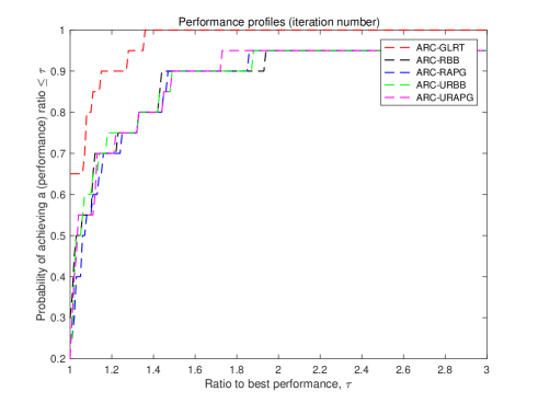
Figure 1: Performance profiles for iteration number for ARC-GLRT, ARC-RBB, ARC-RAPG, ARC-URBB and ARC-URAPG on the CUTEst problems

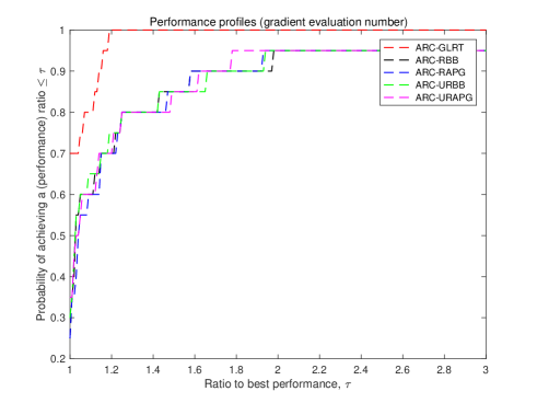
Figure 2: Performance profiles for gradient evaluations for ARC-GLRT, ARC-RBB, ARC-RAPG, ARC-URBB and ARC-URAPG on the CUTEst problems

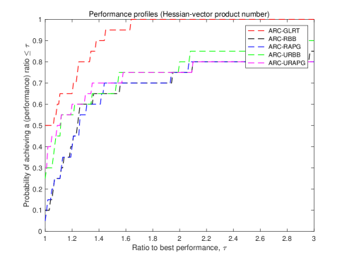
Figure 3: Performance profiles for Hessian-vector products for ARC-GLRT, ARC-RBB, ARC-RAPG, ARC-URBB and ARC-URAPG on the CUTEst problems

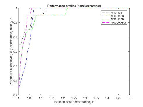
Figure 4: Performance profiles for iteration number for ARC-RBB, ARC-RAPG, ARC-URBB and ARC-URAPG on the CUTEst problems

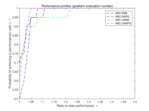
Figure 5: Performance profiles for gradient evaluation for ARC-RBB, ARC-RAPG, ARC-URBB and ARC-URAPG on the CUTEst problems

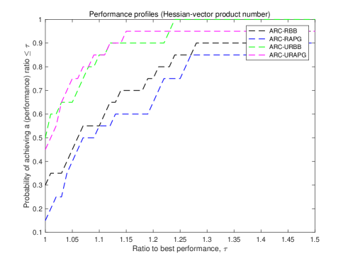
Figure 6: Performance profiles for Hessian-vector products for ARC-RBB, ARC-RAPG, ARC-URBB and ARC-URAPG on the CUTEst problems

To investigate the numerical results more clearly, we illustrate the experiments by performance profiles Figures 1–3 (dolan2002benchmarking ). According to the performs profiles, although ARC-GLRT has the best performance, the iteration numbers and the gradient evaluation numbers of ARC-URBB and ARC-URAPG are less than 2 times of those by ARC-GLRT on over 95% of the tests, and Hessian-vector product number of ARC-URBB is less than 2 times of those by ARC-GLRT on about 85% of the tests. Noting that ARC-URBB, ARC-URAPG, ARC-RBB and ARC-RAPG have the similar performance, we thus plot the performance profiles on test problems for these 4 algorithms in Figures 4–6. We find ARC-URAPG has the best iteration number and gradient evaluation number, and both ARC-URBB and ARC-URAPG have better Hessian-vector product number.

We also investigate the numerical results for all 10 implementations with different initializations, in order to show the advantages of the new algorithms more comprehensively. Table LABEL:tab:cutestfull reports the number that ARC-URBB or ARC-URAPG outperforms ARC-GLRT, ARC-RBB and ARC-RAPG out of the 10 realizations for each problem. It shows our algorithms frequently outperform ARC-GLRT, ARC-RBB and ARC-RAPG in iteration number, number of Hessian-vector products and gradient evaluations.

Table 1: Results on the CUTEst problems

Problem	Method	$n_{i}$	$n_{\text{prod}}$	$n_{f}$	$n_{g}$	$n_{\text{eig}}$	$f^{*}$	time	time${}_{\text{eig}}$	time${}_{\text{loop}}$
BROYDN7D	ARC-GLRT	42.7	828.9	43.7	35.6	-	2.42e+02	0.340	-	0.340
(1000)	ARC-RBB	43.6	946.9	44.6	36.3	17.4	2.40e+02	1.071	0.681	0.390
	ARC-RAPG	43.7	933.5	44.7	36.2	17.9	2.39e+02	1.100	0.701	0.399
	ARC-URBB	43.8	933.2	44.8	36.4	17.9	2.39e+02	1.059	0.688	0.371
	ARC-URAPG	43.4	845.8	44.4	35.9	17.2	2.39e+02	1.058	0.664	0.394
BRYBND	ARC-GLRT	34.3	1575.5	35.3	29.3	-	2.73e+01	0.487	-	0.487
(1000)	ARC-RBB	29.8	1314.3	30.8	25.7	6.5	2.73e+01	1.352	0.946	0.406
	ARC-RAPG	29.8	1288.9	30.8	25.7	6.5	2.73e+01	1.426	1.005	0.421
	ARC-URBB	29.8	1278.7	30.8	25.7	6.5	2.73e+01	1.349	0.956	0.394
	ARC-URAPG	29.8	1262.1	30.8	25.7	6.5	2.73e+01	1.376	0.975	0.402
CHAINWOO	ARC-GLRT	203.5	5462.5	204.5	152.7	-	1.07e+03	1.576	-	1.576
(1000)	ARC-RBB	293.1	10705.2	294.1	218.7	172.5	1.17e+03	26.495	23.215	3.280
	ARC-RAPG	299.5	10625.8	300.5	225.4	178.4	1.17e+03	27.363	23.841	3.522
	ARC-URBB	291.4	8363.3	292.4	219.4	168.0	1.17e+03	26.276	23.553	2.723
	ARC-URAPG	303.4	8683.5	304.4	227.9	178.9	1.16e+03	26.534	23.434	3.099
DIXMAANF	ARC-GLRT	23.8	599.6	24.8	22.6	-	1.00e+00	0.421	-	0.421
(1500)	ARC-RBB	22.1	572.6	23.1	21.2	10.1	1.00e+00	1.391	0.964	0.427
	ARC-RAPG	22.2	543.8	23.2	21.1	10.2	1.00e+00	1.391	0.969	0.423
	ARC-URBB	22.6	535.3	23.6	21.5	10.6	1.00e+00	1.415	1.009	0.406
	ARC-URAPG	22.3	477.2	23.3	21.2	10.3	1.00e+00	1.385	0.974	0.412
DIXMAANG	ARC-GLRT	24.9	606.7	25.9	23.0	-	1.00e+00	0.413	-	0.413
(1500)	ARC-RBB	24.6	652.8	25.6	22.6	11.0	1.00e+00	1.446	0.982	0.464
	ARC-RAPG	23.7	597.5	24.7	22.2	10.1	1.00e+00	1.378	0.927	0.451
	ARC-URBB	23.0	418.1	24.0	21.9	9.8	1.00e+00	1.270	0.912	0.358
	ARC-URAPG	23.3	441.9	24.3	22.0	10.0	1.00e+00	1.274	0.902	0.372
DIXMAANH	ARC-GLRT	29.6	680.8	30.6	25.9	-	1.00e+00	0.461	-	0.461
(1500)	ARC-RBB	30.7	696.6	31.7	26.2	13.3	1.00e+00	1.705	1.186	0.519
	ARC-RAPG	30.5	664.4	31.5	26.1	13.1	1.00e+00	1.696	1.189	0.507
	ARC-URBB	30.5	625.3	31.5	26.0	13.1	1.00e+00	1.659	1.178	0.480
	ARC-URAPG	30.5	619.2	31.5	26.0	13.4	1.00e+00	1.681	1.198	0.483
DIXMAANJ	ARC-GLRT	43.7	4519.5	44.7	37.6	-	1.00e+00	2.311	-	2.311
(1500)	ARC-RBB	48.7	2952.9	49.7	42.4	30.3	1.00e+00	33.409	31.727	1.682
	ARC-RAPG	51.1	3324.3	52.1	43.5	33.1	1.00e+00	37.646	35.873	1.774
	ARC-URBB	50.1	2937.5	51.1	43.5	32.4	1.00e+00	35.312	33.738	1.574
	ARC-URAPG	49.2	2743.4	50.2	42.7	31.3	1.00e+00	33.913	32.392	1.521
DIXMAANK	ARC-GLRT	51.1	4883.9	52.1	43.2	-	1.00e+00	2.458	-	2.458
(1500)	ARC-RBB	63.1	4382.3	64.1	53.1	42.9	1.00e+00	40.483	38.208	2.275
	ARC-RAPG	63.9	4453.5	64.9	53.3	43.8	1.00e+00	41.436	39.114	2.322
	ARC-URBB	60.7	3523.5	61.7	51.5	41.1	1.00e+00	39.471	37.603	1.868
	ARC-URAPG	62.4	3962.9	63.4	52.5	42.4	1.00e+00	40.038	37.941	2.097
DIXMAANL	ARC-GLRT	57.7	4569.5	58.7	47.6	-	1.00e+00	2.334	-	2.334
(1500)	ARC-RBB	65.2	4126.9	66.2	55.0	40.9	1.00e+00	40.609	38.454	2.155
	ARC-RAPG	66.0	4103.8	67.0	55.1	42.1	1.00e+00	40.438	38.255	2.183
	ARC-URBB	61.3	3398.6	62.3	52.2	37.3	1.00e+00	37.372	35.571	1.801
	ARC-URAPG	65.4	3721.6	66.4	54.6	41.3	1.00e+00	39.836	37.842	1.995
EXTROSNB	ARC-GLRT	1824.2	54022.6	1825.2	1274.9	-	1.47e-08	16.641	-	16.641
(1000)	ARC-RBB	1344.0	192873.0	1345.0	1094.9	1236.4	2.99e-06	72.713	12.047	60.666
	ARC-RAPG	1341.0	192160.7	1342.0	1097.3	1234.1	2.99e-06	71.442	11.863	59.579
	ARC-URBB	1383.9	198543.3	1384.9	1129.2	1276.2	2.99e-06	73.391	12.177	61.215
	ARC-URAPG	1397.9	200543.8	1398.9	1121.8	1291.3	2.98e-06	73.764	12.293	61.471
FLETCHCR	ARC-GLRT	1969.9	42563.3	1970.9	1327.2	-	1.20e+00	12.710	-	12.710
(1000)	ARC-RBB	1982.0	53970.1	1983.0	1357.0	774.8	1.20e+00	38.237	13.914	24.324
	ARC-RAPG	1984.0	53642.5	1985.0	1368.1	787.8	1.20e+00	38.062	13.562	24.500
	ARC-URBB	1980.8	52054.4	1981.8	1365.5	782.0	1.20e+00	38.458	14.402	24.056
	ARC-URAPG	1976.8	51214.6	1977.8	1361.9	771.3	1.20e+00	38.390	14.234	24.156
FREUROTH	ARC-GLRT	36.7	366.1	37.7	30.3	-	1.17e+05	0.302	-	0.302
(1000)	ARC-RBB	33.8	1122.4	34.8	30.2	21.2	1.17e+05	0.697	0.205	0.492
	ARC-RAPG	36.0	1371.1	37.0	31.6	23.5	1.17e+05	0.787	0.222	0.565
	ARC-URBB	36.5	1400.4	37.5	30.2	24.0	1.17e+05	0.885	0.247	0.639
	ARC-URAPG	34.8	1207.6	35.8	30.1	22.0	1.17e+05	0.810	0.219	0.591
GENHUMPS	ARC-GLRT	1702.9	50838.9	1703.9	1039.5	-	8.73e-13	15.912	-	15.912
(1000)	ARC-RBB	1525.5	41837.4	1526.5	922.5	9.3	7.06e-12	20.876	0.206	20.670
	ARC-RAPG	1525.4	41841.4	1526.4	922.4	9.3	8.90e-12	19.249	0.218	19.030
	ARC-URBB	1525.5	41729.6	1526.5	922.6	9.3	8.34e-12	22.510	0.199	22.311
	ARC-URAPG	1525.4	41762.7	1526.4	922.5	9.3	1.44e-11	21.270	0.200	21.071
GENROSE	ARC-GLRT	1058.6	20703.8	1059.6	711.7	-	1.00e+00	2.818	-	2.818
(500)	ARC-RBB	1079.7	28236.6	1080.7	736.9	166.5	1.00e+00	4.092	0.944	3.149
	ARC-RAPG	1151.5	29887.7	1152.5	780.7	191.6	1.00e+00	3.594	0.863	2.732
	ARC-URBB	1081.1	28124.1	1082.1	737.5	164.3	1.00e+00	3.848	0.890	2.958
	ARC-URAPG	1083.4	27979.1	1084.4	737.1	169.7	1.00e+00	4.268	1.005	3.263
NONCVXU2	ARC-GLRT	65.5	8065.7	66.5	61.5	-	2.32e+03	2.083	-	2.083
(1000)	ARC-RBB	127.5	7660.5	128.5	122.1	124.5	2.32e+03	78.082	75.564	2.518
	ARC-RAPG	122.4	7637.8	123.4	118.9	119.6	2.32e+03	77.664	75.163	2.501
	ARC-URBB	123.4	7845.9	124.4	119.6	120.6	2.32e+03	78.858	76.286	2.571
	ARC-URAPG	113.8	7211.2	114.8	109.9	111.0	2.32e+03	71.320	69.111	2.209
NONCVXUN	ARC-GLRT	300.9	224970.5	301.9	294.5	-	2.32e+03	49.239	-	49.239
(1000)	ARC-RBB	2025.5	283403.7	2026.5	2018.8	2021.6	2.32e+03	1414.201	1346.432	67.769
	ARC-RAPG	2116.6	295837.9	2117.6	2109.8	2112.9	2.32e+03	1479.271	1407.690	71.581
	ARC-URBB	2483.0	350646.4	2484.0	2477.1	2479.3	2.32e+03	1734.238	1650.711	83.527
	ARC-URAPG	2105.2	294676.3	2106.2	2098.3	2101.3	2.32e+03	1466.452	1393.276	73.176
OSCIPATH	ARC-GLRT	39.3	6079.9	40.3	31.3	-	3.12e-01	0.516	-	0.516
(500)	ARC-RBB	56.4	5658.1	57.4	49.5	27.8	3.12e-01	5.502	5.204	0.298
	ARC-RAPG	57.0	5747.5	58.0	49.6	28.1	3.12e-01	5.702	5.348	0.354
	ARC-URBB	58.7	6007.2	59.7	52.0	30.5	3.12e-01	6.163	5.845	0.318
	ARC-URAPG	57.3	5799.2	58.3	50.8	28.7	3.12e-01	5.866	5.532	0.334
TOINTGSS	ARC-GLRT	19.2	118.6	20.2	14.1	-	1.00e+01	0.119	-	0.119
(1000)	ARC-RBB	15.4	368.2	16.4	12.2	10.3	1.00e+01	0.269	0.086	0.183
	ARC-RAPG	15.9	494.7	16.9	12.4	10.9	1.00e+01	0.296	0.081	0.215
	ARC-URBB	15.0	322.9	16.0	11.8	10.0	1.00e+01	0.233	0.076	0.156
	ARC-URAPG	15.6	372.6	16.6	12.5	10.6	1.00e+01	0.255	0.082	0.173
TQUARTIC	ARC-GLRT	63.9	282.1	64.9	52.9	-	2.37e-14	0.363	-	0.363
(1000)	ARC-RBB	71.5	838.6	72.5	55.6	6.9	1.99e-13	0.598	0.084	0.513
	ARC-RAPG	71.0	934.8	72.0	55.4	6.6	8.58e-11	0.674	0.090	0.584
	ARC-URBB	71.3	566.7	72.3	55.6	6.9	1.04e-10	0.521	0.091	0.431
	ARC-URAPG	72.3	926.4	73.3	56.5	6.7	3.79e-10	0.639	0.087	0.552
WOODS	ARC-GLRT	286.4	4542.6	287.4	210.2	-	8.66e-15	1.561	-	1.561
(1000)	ARC-RBB	382.8	9574.8	383.8	264.5	6.2	1.88e-12	3.733	0.067	3.666
	ARC-RAPG	381.3	9426.5	382.3	263.9	5.5	3.15e-14	3.340	0.051	3.288
	ARC-URBB	382.2	9486.3	383.2	264.2	6.1	1.67e-14	3.722	0.067	3.655
	ARC-URAPG	381.7	9542.6	382.7	264.6	6.3	1.67e-12	3.833	0.068	3.765

Table 2: The number of times ARC-URBB (or ARC-URAPG) performs better than the other three algorithms in 10 realizations.

Problem	Index	ARC-URBB			ARC-URAPG
		ARC-GLRT	ARC-RBB	ARC-RAPG	ARC-GLRT	ARC-RBB	ARC-RAPG
BROYDN7D	$n_{i}$	4	5	2	4	6	4
	$n_{\text{prod}}$	4	5	6	5	8	6
	$n_{g}$	3	3	1	4	4	2
BRYBND	$n_{i}$	10	0	0	10	0	0
	$n_{\text{prod}}$	7	7	4	7	9	6
	$n_{g}$	10	0	0	10	0	0
CHAINWOO	$n_{i}$	0	5	7	0	3	5
	$n_{\text{prod}}$	0	10	9	0	10	9
	$n_{g}$	0	6	6	0	2	5
DIXMAANF	$n_{i}$	7	0	2	6	1	0
	$n_{\text{prod}}$	5	6	5	7	6	7
	$n_{g}$	6	0	1	6	2	0
DIXMAANG	$n_{i}$	7	5	4	6	6	3
	$n_{\text{prod}}$	10	10	9	9	10	9
	$n_{g}$	6	4	4	7	6	2
DIXMAANH	$n_{i}$	3	2	2	4	2	1
	$n_{\text{prod}}$	7	6	5	6	7	6
	$n_{g}$	4	2	2	3	2	1
DIXMAANJ	$n_{i}$	1	5	5	1	5	4
	$n_{\text{prod}}$	10	7	7	10	9	7
	$n_{g}$	1	6	5	1	3	3
DIXMAANK	$n_{i}$	0	7	7	1	5	4
	$n_{\text{prod}}$	9	7	9	8	8	7
	$n_{g}$	0	5	7	0	5	5
DIXMAANL	$n_{i}$	4	7	6	2	4	5
	$n_{\text{prod}}$	8	8	8	9	7	7
	$n_{g}$	2	6	6	1	3	5
EXTROSNB	$n_{i}$	10	3	3	10	2	3
	$n_{\text{prod}}$	0	3	3	0	2	3
	$n_{g}$	10	3	3	10	5	5
FLETCHCR	$n_{i}$	5	4	5	5	5	6
	$n_{\text{prod}}$	4	8	8	5	9	8
	$n_{g}$	2	2	6	2	2	9
FREUROTH	$n_{i}$	5	4	4	7	3	5
	$n_{\text{prod}}$	0	5	7	0	4	6
	$n_{g}$	5	5	6	4	4	7
GENHUMPS	$n_{i}$	10	1	0	10	2	0
	$n_{\text{prod}}$	10	7	8	10	7	7
	$n_{g}$	10	0	0	10	1	0
GENROSE	$n_{i}$	3	5	4	3	4	4
	$n_{\text{prod}}$	1	5	5	1	6	5
	$n_{g}$	3	4	6	3	5	5
NONCVXU2	$n_{i}$	0	7	6	0	9	7
	$n_{\text{prod}}$	6	4	6	7	8	6
	$n_{g}$	0	5	6	0	8	7
NONCVXUN	$n_{i}$	0	4	4	0	7	5
	$n_{\text{prod}}$	1	4	4	2	7	5
	$n_{g}$	0	4	4	0	7	5
OSCIPATH	$n_{i}$	0	4	3	0	4	5
	$n_{\text{prod}}$	5	4	3	5	4	5
	$n_{g}$	0	3	3	0	5	4
TOINTGSS	$n_{i}$	6	1	3	7	1	1
	$n_{\text{prod}}$	1	5	9	0	6	9
	$n_{g}$	7	2	4	7	2	1
TQUARTIC	$n_{i}$	4	3	4	3	4	4
	$n_{\text{prod}}$	0	9	10	0	4	7
	$n_{g}$	5	3	4	3	4	4
WOODS	$n_{i}$	0	6	1	0	4	4
	$n_{\text{prod}}$	0	6	4	0	6	3
	$n_{g}$	0	6	1	0	4	2

6 Conclusion

In this paper, we propose a new convex reformulation for the subproblem of the cubic regularization methods. Based on our reformulation, we propose a variant of the non-adaptive CR algorithm that admits an iteration complexity ${\mathcal{O}}(\epsilon_{g}^{-3/2})$ to find an $(\epsilon_{g},\sqrt{L\epsilon_{g}})$ stationary point. Moreover, we show that an operation complexity bound of our algorithm is ${\mathcal{\tilde{O}}}(\epsilon_{g}^{-7/4})$ when the subproblems are solved by Nesterov’s accelerated gradient method and the approximated eigenvalues are computed by the Lanczos procedure. We also propose a variant of the ARC algorithm with similar complexity guarantees. Both of our iteration and operation complexity bounds match the best known bounds in the literature for algorithms that based on first- and second-order information. Numerical experiments on the ARC equipped with our reformulation for solving subproblems also illustrate the effectiveness of our approach.

For future research, we would like to explore if our reformulation can be extended to solve auxiliary problems in tensor methods for unconstrained optimization (birgin2017worst ; jiang2020unified ; nesterov2021implementable ; grapiglia2021inexact ), which were shown to have fast global convergence guarantees. It is well known that the auxiliary problem in the model function in each iteration of the tensor method is a regularized $p$-th order Taylor approximation, which is difficult to solve. Two recent works nesterov2021implementable ; grapiglia2021inexact show that for $p=3$ and convex minimization problems, the Tensor model can be solved by an adaptive Bregman proximal gradient method, where each subproblem is of form

$$\min_{x}c^{\top}x+\frac{1}{2}x^{\top}Ax+\frac{\gamma}{3+\nu}\|x\|^{3+\nu},\text{ with }A\succeq 0.$$

It will be interesting to see if the methods in nesterov2021implementable ; grapiglia2021inexact can be extended to nonconvex minimization problems and still have similar subproblems, and if our reformulation can be extended to solving these subproblems.

7 Appendix

7.1 Proofs for Lemma 1

In this case, $s_{k}$ is approximately computed by (7) or (9). Let $\sigma=L/2$ for Algorithm 1 and $\sigma=\sigma_{k}$ for Algorithm 2. Noting that $d_{k}=s_{k}$, by (13), we have

$$\left\|g_{k}+H_{k}d_{k}+3\epsilon_{E}d_{k}+\sigma\|d_{k}\|d_{k}\right\|\leq\epsilon_{S}.$$ (19)

Since

$$\left\|g_{k}+H_{k}d_{k}+3\epsilon_{E}d_{k}+\sigma\|d_{k}\|d_{k}\right\|\geq\left\|g_{k}+H_{k}d_{k}\right\|-3\epsilon_{E}\|d_{k}\|-\sigma\|d_{k}\|^{2},$$

we have

$$\left\|g_{k}+H_{k}d_{k}\right\|\leq\epsilon_{S}+3\epsilon_{E}\|d_{k}\|+\sigma\|d_{k}\|^{2}.$$ (20)

Due to $\alpha_{k}\leq\lambda_{\text{min}}(H_{k})+\epsilon_{E}$ and $\alpha_{k}\geq-\epsilon_{E}$, we have

$$\lambda_{\text{min}}(H_{k})\geq-2\epsilon_{E}.$$ (21)

Using (19), we have

$$g_{k}^{\top}d_{k}+d_{k}^{\top}H_{k}d_{k}+3\epsilon_{E}\|d_{k}\|^{2}+\sigma\|d_{k}\|^{3} \leq\left\|g_{k}+H_{k}d_{k}+3\epsilon_{E}d_{k}+\sigma\|d_{k}\|d_{k}\right\|\cdot\|d_{k}\|$$ (22)

$$\leq\epsilon_{S}\|d_{k}\|.$$

Then we have

$$g_{k}^{\top}d_{k} \overset{\eqref{eq:case2-1-gd-dHd}}{\leq}\epsilon_{S}\|d_{k}\|-d_{k}^{\top}H_{k}d_{k}-3\epsilon_{E}\|d_{k}\|^{2}-\sigma\|d_{k}\|^{3}$$ (23)

$$=\epsilon_{S}\|d_{k}\|-(d_{k}^{\top}H_{k}d_{k}+3\epsilon_{E}\|d_{k}\|^{2})-\sigma\|d_{k}\|^{3}$$

$$\overset{\eqref{eq:case2-1-lambda}}{\leq}\epsilon_{S}\|d_{k}\|-\epsilon_{E}\|d_{k}\|^{2}-\sigma\|d_{k}\|^{3},$$

By (22), we also have

$$d_{k}^{\top}H_{k}d_{k}\leq-g_{k}^{\top}d_{k}-3\epsilon_{E}\|d_{k}\|^{2}-\sigma\|d_{k}\|^{3}+\epsilon_{S}\|d_{k}\|.$$ (24)

Hence we obtain

$$m(d_{k}) =g_{k}^{\top}d_{k}+\frac{1}{2}d_{k}^{\top}H_{k}d_{k}+\frac{\sigma}{3}\|d_{k}\|^{3}$$

$$\overset{\eqref{eq:case2-1-dHd}}{\leq}g_{k}^{\top}d_{k}-\frac{1}{2}g_{k}^{\top}d_{k}-\frac{3}{2}\epsilon_{E}\|d_{k}\|^{2}-\frac{\sigma}{2}\|d_{k}\|^{3}+\frac{1}{2}\epsilon_{S}\|d_{k}\|+\frac{\sigma}{3}\|d_{k}\|^{3}$$

$$=\frac{1}{2}g_{k}^{\top}d_{k}-\frac{3}{2}\epsilon_{E}\|d_{k}\|^{2}+\frac{1}{2}\epsilon_{S}\|d_{k}\|-\frac{\sigma}{6}\|d_{k}\|^{3}$$

$$\overset{\eqref{eq:case2-1-gd}}{\leq}\frac{1}{2}\epsilon_{S}\|d_{k}\|-\frac{\sigma}{2}\|d_{k}\|^{3}-2\epsilon_{E}\|d_{k}\|^{2}+\frac{1}{2}\epsilon_{S}\|d_{k}\|-\frac{\sigma}{6}\|d_{k}\|^{3}$$

$$=-\frac{2\sigma}{3}\|d_{k}\|^{3}-2\epsilon_{E}\|d_{k}\|^{2}+\epsilon_{S}\|d_{k}\|,$$

or equivalently,

$$-m(d_{k})\geq\frac{2\sigma}{3}\|d_{k}\|^{3}+2\epsilon_{E}\|d_{k}\|^{2}-\epsilon_{S}\|d_{k}\|.$$

Due to $\epsilon_{S}=\epsilon_{E}^{2}/L$ as in Condition 2, it follows that

$$-m(d_{k})\geq\frac{2\sigma}{3}\|d_{k}\|^{3}+2\epsilon_{E}\|d_{k}\|^{2}-\frac{\epsilon_{E}^{2}}{L}\|d_{k}\|.$$ (25)

Now suppose that $x_{k}+d_{k}$ is not an $(\epsilon_{g},\sqrt{L\epsilon_{g}})$ stationary point. We then have either (i) $\|\nabla f(x_{k}+d_{k})\|>\epsilon_{g}$, or (ii) $\|\nabla f(x_{k}+d_{k})\|\leq\epsilon_{g},~{}\lambda_{\min}(\nabla^{2}f(x_{k}+d_{k}))<-\sqrt{L\epsilon_{g}}$. Let us consider the following cases (i) and (ii) separately.

• Using (20), Taylor expansion for $\nabla f(x_{k}+d_{k})$ and (11), we have

  $$\begin{array}[]{rcl}\|\nabla f(x_{k}+d_{k})\|&\leq&\|g_{k}+H_{k}d_{k}\|+\frac{L}{2}\|d_{k}\|^{2}\\ &\leq&\epsilon_{S}+3\epsilon_{E}\|d_{k}\|+(\sigma+\frac{L}{2})\|d_{k}\|^{2},\end{array}$$ (26)

  where the first inequality follows from Lemma 1 in nesterov2006cubic . Using $\|\nabla f(x_{k}+d_{k})\|>\epsilon_{g}$ and (26), we obtain

  $$\epsilon_{g}\leq\epsilon_{S}+3\epsilon_{E}\|d_{k}\|+(\sigma+\frac{L}{2})\|d_{k}\|^{2}.$$

  This gives

  $$\|d_{k}\|\geq\frac{-3\epsilon_{E}+\sqrt{9\epsilon_{E}^{2}-4(\sigma+\frac{L}{2})(\epsilon_{S}-\epsilon_{g})}}{2\sigma+L}\quad\text{or}\quad\|d_{k}\|\leq\frac{-3\epsilon_{E}-\sqrt{9\epsilon_{E}^{2}-4(\sigma+\frac{L}{2})(\epsilon_{S}-\epsilon_{g})}}{2\sigma+L}.$$

  where the second case is discarded since $\|d_{k}\|\geq 0$. Due to $\epsilon_{S}=\epsilon_{E}^{2}/L$ and $\epsilon_{g}=\epsilon_{E}^{2}/L$ in Condition 2, we further have

  $$\|d_{k}\|\geq\frac{-3\epsilon_{E}+\sqrt{25\epsilon_{E}^{2}+(32\sigma/L)\epsilon_{E}^{2}}}{2\sigma+L}.$$ (27)

  • For Algorithm 1, due to $\sigma=L/2$, (27) yields

    $$\|d_{k}\|\geq\frac{3}{2L}\epsilon_{E},$$

    Therefore, using $\sigma=L/2$, we have

    $$-m(d_{k})\overset{\eqref{eq:case1-mdk}}{\geq}\frac{33\epsilon_{E}^{3}}{8L^{2}}.$$

  • Note that from Lemma 7, we have $\sigma=\sigma_{k}\leq\max\{\sigma_{0},\frac{\gamma L}{2}\}$ for Algorithm 2. Therefore if $\sigma\geq L/2$, (27) yields

    $$\|d_{k}\|\geq\frac{3}{(\max\{\gamma,2\sigma_{0}/L\}+1)L}\epsilon_{E},$$ (28)

    and if $\sigma<L/2$, (27) yields

    $$\|d_{k}\|\geq\frac{1}{L}\epsilon_{E},$$ (29)

    Using (27), we claim the following inequality holds,

    $$\frac{2\sigma}{3}\|d_{k}\|^{2}+2\epsilon_{E}\|d_{k}\|-\frac{\epsilon_{E}^{2}}{L}\geq\frac{3\epsilon_{E}^{2}}{L},$$ (30)

    provided $\sigma>0$. Now combining (25), (28), (29) and (30), we have

    $$-m(d_{k})\geq\frac{3\epsilon_{E}^{2}}{L}\|d_{k}\|\geq\min\left\{\frac{3}{\max\{\gamma,2\sigma_{0}/L\}+1},1\right\}\cdot\frac{3\epsilon_{E}^{3}}{L^{2}}$$

    Indeed, to prove inequality (30), we only need to show, using (27),

    $$\frac{2(\sqrt{25+32a}-3)^{2}}{3(4a+4+1/a)}+\frac{2(\sqrt{25+32a}-3)}{2a+1}=\frac{2}{3}\frac{32a^{2}+16a+3\sqrt{25+32a}-9}{(2a+1)^{2}}\geq 4,$$

    for $a=\sigma/L>0$. Note that the above inequality is equivalent to

    $$\psi(a)=8a^{2}-8a+3\sqrt{25+32a}-15\geq 0.$$

    As $\psi(0)=0$, it suffices to show

    $$\psi^{\prime}(a)=16a-8+\frac{48}{\sqrt{25+32a}}>0,~{}\forall a\geq 0.$$

    This holds because

    $$\psi^{\prime\prime}(a)=16-48\frac{16}{(\sqrt{25+32a})^{3}}=16(1-\frac{48}{(\sqrt{25+32a})^{3}})\geq 16(1-\frac{48}{125})>0,~{}\forall a\geq 0,$$

    and $\psi^{\prime}(0)=\frac{8}{5}\geq 0$.

• By Assumption 1 and (21), we have

  $$\lambda_{\min}(\nabla^{2}f(x_{k}+d_{k}))\geq\lambda_{\min}(H_{k})-L\|d_{k}\|\geq-2\epsilon_{E}-L\|d_{k}\|.$$ (31)

  Using $\lambda_{\min}(\nabla^{2}f(x_{k}+d_{k}))\leq-\sqrt{L\epsilon_{g}}$ and (31), we obtain

  $$-2\epsilon_{E}-L\|d_{k}\|\leq-\sqrt{L\epsilon_{g}}.$$

  This, together with $\epsilon_{E}=\sqrt{L\epsilon_{g}}/3$, implies

  $$\|d_{k}\|\geq\frac{\sqrt{L\epsilon_{g}}-2\epsilon_{E}}{L}=\frac{\epsilon_{E}}{L}.$$ (32)

  It follows that

  $$-m(d_{k}) \overset{\eqref{eq:case1-mdk}}{\geq}\frac{2\sigma}{3}\|d_{k}\|^{3}+2\epsilon_{E}\|d_{k}\|^{2}-\frac{\epsilon_{E}^{2}}{L}\|d_{k}\|$$

  $$\overset{\eqref{eq:case2-dkbd}}{\geq}\left(0+2\epsilon_{E}\left(\frac{\epsilon_{E}}{L}\right)-\frac{\epsilon_{E}^{2}}{L}\right)\|d_{k}\|$$

  $$\overset{\eqref{eq:case2-dkbd}}{\geq}\frac{\epsilon_{E}^{3}}{L^{2}}.$$

Combining (i) and (ii), we complete the proof.

7.2 Proofs for Lemma 2

In this case, $d_{k}$ is generated by either line 13 or line 16 of Algorithm 1 (Algorithm 2, respectively), depending on the norm of $s_{k}$ returned by approximately solving (8) ((10), respectively). Let $\sigma=L/2$ for Algorithm 1 and $\sigma=\sigma_{k}$ for Algorithm 2. We prove the results twofold.

• When $\sigma\|s_{k}\|+\alpha_{k}\geq 0$, we must have $[\sigma\|s_{k}\|+\alpha_{k}]_{+}=\sigma\|s_{k}\|+\alpha_{k}$. Note that

  $$\nabla\tilde{m}_{k}^{r}(s_{k})=g_{k}+H_{k}s_{k}+(2\epsilon_{E}-\alpha_{k})s_{k}+\left[\sigma\|s_{k}\|+\alpha_{k}\right]_{+}{s_{k}}.$$ (33)

  Using (14) and $d_{k}=s_{k}$, we obtain

  $$g_{k}^{\top}d_{k}+d_{k}^{\top}H_{k}d_{k}+(2\epsilon_{E}-\alpha_{k})\|d_{k}\|^{2}+\left[\sigma\|d_{k}\|+\alpha_{k}\right]_{+}{\|d_{k}\|^{2}}$$ (34)

  $$\leq \left\|g_{k}+H_{k}d_{k}+(2\epsilon_{E}-\alpha_{k})d_{k}+\left[\sigma\|d_{k}\|+\alpha_{k}\right]_{+}{d_{k}}\right\|\cdot\|d_{k}\|$$

  $$\leq \epsilon_{S}\|d_{k}\|.$$

  Since $\alpha_{k}\leq\lambda_{\text{min}}(H_{k})+\epsilon_{E}$, we have $H_{k}-\alpha_{k}I+2\epsilon_{E}I\succeq 0$ and thus

  $$d_{k}^{\top}H_{k}d_{k}+(2\epsilon_{E}-\alpha_{k})\|d_{k}\|^{2}\geq 0.$$ (35)

  Noting that $\left[\sigma\|s_{k}\|+\alpha_{k}\right]_{+}\geq 0$, we have from (34) and (35) that

  $$g_{k}^{\top}d_{k}\leq\epsilon_{S}\|d_{k}\|.$$ (36)

  On the other hand, according to $\sigma\|s_{k}\|+\alpha_{k}\geq 0$ and (34), we have

  $$d_{k}^{\top}H_{k}d_{k} \leq-g_{k}^{\top}d_{k}+(\alpha_{k}-2\epsilon_{E})\|d_{k}\|^{2}-\sigma\|d_{k}\|^{3}-\alpha_{k}\|d_{k}\|^{2}+\epsilon_{S}\|d_{k}\|$$ (37)

  $$=-g_{k}^{\top}d_{k}-\sigma\|d_{k}\|^{3}-2\epsilon_{E}\|d_{k}\|^{2}+\epsilon_{S}\|d_{k}\|.$$

  Since $d_{k}=s_{k}$, and $\alpha_{k}\leq-\epsilon_{E}$, from $\sigma\|s_{k}\|+\alpha_{k}\geq 0$ we obtain

  $$\|d_{k}\|\geq-\frac{\alpha_{k}}{\sigma}\geq\frac{\epsilon_{E}}{\sigma}.$$ (38)

  We further have

  $$m(d_{k}) =g_{k}^{\top}d_{k}+\frac{1}{2}d_{k}^{\top}H_{k}d_{k}+\frac{\sigma}{3}\|d_{k}\|^{3}$$

  $$\overset{\eqref{eq:case2-2-dHd}}{\leq}g_{k}^{\top}d_{k}-\frac{1}{2}g_{k}^{\top}d_{k}-\frac{\sigma}{2}\|d_{k}\|^{3}-\epsilon_{E}\|d_{k}\|^{2}\ +\frac{1}{2}\epsilon_{S}\|d_{k}\|+\frac{\sigma}{3}\|d_{k}\|^{3}$$

  $$=\frac{1}{2}g_{k}^{\top}d_{k}+\frac{1}{2}\epsilon_{S}\|d_{k}\|-\epsilon_{E}\|d_{k}\|^{2}-\frac{\sigma}{6}\|d_{k}\|^{3}$$

  $$\overset{\eqref{eq:case2-2-gd}}{\leq}\frac{1}{2}\epsilon_{S}\|d_{k}\|+\frac{1}{2}\epsilon_{S}\|d_{k}\|-\epsilon_{E}\|d_{k}\|^{2}-\frac{\sigma}{6}\|d_{k}\|^{3}$$

  $$=-\frac{\sigma}{6}\|d_{k}\|^{3}-\epsilon_{E}\|d_{k}\|^{2}+\epsilon_{S}\|d_{k}\|.$$

  This gives

  $$-m(d_{k})\geq\frac{\sigma}{6}\|d_{k}\|^{3}+\epsilon_{E}\|d_{k}\|^{2}-\epsilon_{S}\|d_{k}\|.$$ (39)

  Thus the desired bound holds immediately for Algorithm 1.

  Now consider Algorithm 2. Similar to the proof for Lemma 1, we consider two cases $\|\nabla f(x_{k}+d_{k})\|>\epsilon_{g}$, and $\|\nabla f(x_{k}+d_{k})\|\leq\epsilon_{g},~{}\lambda_{\min}(\nabla^{2}f(x_{k}+d_{k}))<-\sqrt{L\epsilon_{g}}$. For the latter case, similar to case (ii) in the proof of Lemma 1, from Lipschitz continuity of Hessian, we have $\|d_{k}\|\geq\epsilon_{E}/L$. Then due to $\epsilon_{S}=\epsilon_{E}^{2}/L$ in Condition 2, we have $2\epsilon_{E}\|d_{k}\|-\epsilon_{S}\geq 0$ and thus (39) yields

  $$-m(d_{k})\geq\frac{\sigma}{6}\|d_{k}\|^{3}\overset{\eqref{eq:case2-a1}}{\geq}\frac{\epsilon_{E}^{3}}{6\sigma^{2}}.$$

  Now consider the case $\|\nabla f(x_{k}+d_{k})\|>\epsilon_{g}$, whose proof follows a similar idea to that in Lemma 1. Since the subproblem is approximately solved, we have

  $$\|\nabla\tilde{m}_{k}^{r}(d_{k})\|\leq\epsilon_{S}$$

  and thus (33), together with $\sigma\|d_{k}\|+\alpha_{k}\geq 0$, gives

  $$\|g_{k}+H_{k}d_{k}+(2\epsilon_{E}-\alpha_{k})d_{k}+\left[\sigma\|d_{k}\|+\alpha_{k}\right]_{+}{d_{k}}\|=\|g_{k}+H_{k}d_{k}+(2\epsilon_{E}+\sigma\|d_{k}\|){d_{k}}\|\leq\epsilon_{S}.$$

  Hence we have

  $$\epsilon_{g}\leq\|\nabla f(x_{k}+d_{k})\|\leq\|g_{k}+H_{k}\|+\frac{L}{2}\|d_{k}\|^{2}\leq\epsilon_{S}+2\epsilon_{E}\|d_{k}\|+(\sigma+\frac{L}{2})\|d_{k}\|^{2}.$$

  The due to Condition 2, the above quadratic inequality gives

  $$\|d_{k}\|\geq\frac{-2\epsilon_{E}+\sqrt{4\epsilon_{E}^{2}-4(\sigma+L/2)(\epsilon_{S}-\epsilon_{g})}}{2\sigma+L}=\frac{-2\epsilon_{E}+\sqrt{20\epsilon_{E}^{2}+32\sigma\epsilon_{E}^{2}/L}}{2\sigma+L}.$$

  We claim the following inequality holds

  $$\frac{\sigma}{6}\|d_{k}\|^{2}+\epsilon_{E}\|d_{k}\|-\epsilon_{S}\geq\frac{\sigma}{6}\left(\frac{-2\epsilon_{E}+\sqrt{20\epsilon_{E}^{2}+32\sigma\epsilon_{E}^{2}/L}}{2\sigma+L}\right)^{2}+\epsilon_{E}\frac{-2\epsilon_{E}+\sqrt{20\epsilon_{E}^{2}+32\sigma\epsilon_{E}^{2}/L}}{2\sigma+L}-\frac{\epsilon_{E}^{2}}{L}\geq\frac{\epsilon_{E}^{2}}{3L},$$ (40)

  which further gives

  $$-m(d_{k})\geq\frac{1}{3L}\epsilon_{E}^{2}\|d_{k}\|\overset{\eqref{eq:case2-a1}}{\geq}\frac{1}{3\sigma L}\epsilon_{E}^{3}.$$

  Indeed, (40) is equivalent to, by defining $a=\sigma/L$,

  $$\psi(a)=4a\sqrt{5+8a}-8a+3\sqrt{5+8a}-5\geq 0,$$

  which holds since

  $$\frac{1}{8}\psi^{\prime}(a)=\frac{6a+4}{\sqrt{5+8a}}-1\geq 0~{}\Longleftrightarrow~{}36a^{2}+40a+9\geq 0~{}\Longleftrightarrow~{}9(2a+1)^{2}+4a\geq 0~{}\forall a\geq 0,$$

  and $\psi(0)=3\sqrt{5}-5>0.$

• When $\sigma\|s_{k}\|+\alpha_{k}<0$, we have $d_{k}=\frac{1}{2\sigma}w_{k},~{}\alpha_{k}=v_{k}^{\top}H_{k}v_{k}=\frac{w_{k}^{\top}H_{k}w_{k}}{w_{k}^{\top}w_{k}},~{}\|w_{k}\|=|\alpha_{k}|$, and $w_{k}^{\top}g_{k}\leq 0$. It follows that

  $$d_{k}^{\top}H_{k}d_{k}=\frac{1}{4\sigma^{2}}w_{k}^{\top}H_{k}w_{k}=\frac{1}{4\sigma^{2}}\alpha_{k}w_{k}^{\top}w_{k}=\frac{1}{4\sigma^{2}}\alpha_{k}^{3}.$$ (41)

  Since $\alpha_{k}\leq-\epsilon_{E}<0$, we also have

  $$\|d_{k}\|^{3}=\frac{1}{8\sigma^{3}}\|w_{k}\|^{3}=\frac{1}{8\sigma^{3}}|\alpha_{k}|^{3}=-\frac{1}{8\sigma^{3}}\alpha_{k}^{3}.$$ (42)

  Then we have

  $$m(d_{k}) =g_{k}^{\top}d_{k}+\frac{1}{2}d_{k}^{\top}H_{k}d_{k}+\frac{\sigma}{3}\|d_{k}\|^{3}$$

  $$=\frac{1}{2\sigma}g_{k}^{\top}w_{k}+\frac{1}{8\sigma^{2}}\alpha_{k}^{3}-\frac{1}{24\sigma^{2}}\alpha_{k}^{3}$$

  $$\leq\frac{1}{12\sigma^{2}}\alpha_{k}^{3},$$

  where the second equality follows from (41) and (42), and the inequality follows from $w_{k}^{\top}g_{k}\leq 0$. Due to $\alpha_{k}\leq-\epsilon_{E}$, we have

  $$-m(d_{k})\geq-\frac{1}{12\sigma^{2}}\alpha_{k}^{3}\geq\frac{1}{12\sigma^{2}}\epsilon_{E}^{3}.$$

Combining (i) and (ii) and noting $\sigma=L/2$ in Algorithm 1 and $\sigma=\sigma_{k}\in(0,\max\{\sigma_{0},\gamma L/2\})$ (due to Lemma 7) and $\gamma>1$ in Algorithm 2, we complete the proof.

References

• [1] Yurii Nesterov and Boris T Polyak. Cubic regularization of Newton method and its global performance. Mathematical Programming, 108(1):177–205, 2006.
• [2] Coralia Cartis, Nicholas IM Gould, and Philippe L Toint. Adaptive cubic regularisation methods for unconstrained optimization. Part I: motivation, convergence and numerical results. Mathematical Programming, 127(2):245–295, 2011.
• [3] Andreas Griewank. The modification of Newton’s method for unconstrained optimization by bounding cubic terms. Technical report, Technical report NA/12, 1981.
• [4] Coralia Cartis, Nicholas IM Gould, and Philippe L Toint. Adaptive cubic regularisation methods for unconstrained optimization. part ii: worst-case function-and derivative-evaluation complexity. Mathematical programming, 130(2):295–319, 2011.
• [5] Frank E Curtis, Daniel P Robinson, Clément W Royer, and Stephen J Wright. Trust-Region Newton-CG with Strong Second-Order Complexity Guarantees for Nonconvex Optimization. SIAM Journal on Optimization, 31(1):518–544, 2021.
• [6] Naman Agarwal, Zeyuan Allen-Zhu, Brian Bullins, Elad Hazan, and Tengyu Ma. Finding approximate local minima faster than gradient descent. In Proceedings of the 49th Annual ACM SIGACT Symposium on Theory of Computing, pages 1195–1199. ACM, 2017.
• [7] Yair Carmon, John C Duchi, Oliver Hinder, and Aaron Sidford. Accelerated methods for nonconvex optimization. SIAM Journal on Optimization, 28(2):1751–1772, 2018.
• [8] Clément W Royer and Stephen J Wright. Complexity analysis of second-order line-search algorithms for smooth nonconvex optimization. SIAM Journal on Optimization, 28(2):1448–1477, 2018.
• [9] Clément W Royer, Michael O’Neill, and Stephen J Wright. A Newton-CG algorithm with complexity guarantees for smooth unconstrained optimization. Mathematical Programming, 180(1):451–488, 2020.
• [10] Yair Carmon and John C Duchi. Analysis of Krylov subspace solutions of regularized non-convex quadratic problems. In Advances in Neural Information Processing Systems, pages 10705–10715, 2018.
• [11] Yair Carmon and John C Duchi. First-order methods for nonconvex quadratic minimization. SIAM Review, 62(2):395–436, 2020.
• [12] Yair Carmon and John Duchi. Gradient descent finds the cubic-regularized nonconvex Newton step. SIAM Journal on Optimization, 29(3):2146–2178, 2019.
• [13] Rujun Jiang, Man-Chung Yue, and Zhishuo Zhou. An accelerated first-order method with complexity analysis for solving cubic regularization subproblems. Computational Optimization and Applications, 79(2):471–506, 2021.
• [14] Olaf E Flippo and Benjamin Jansen. Duality and sensitivity in nonconvex quadratic optimization over an ellipsoid. European Journal of Operational Research, 94(1):167–178, 1996.
• [15] Nam Ho-Nguyen and Fatma Kılınç-Karzan. A second-order cone based approach for solving the trust-region subproblem and its variants. SIAM Journal on Optimization, 27(3):1485–1512, 2017.
• [16] Jiulin Wang and Yong Xia. A linear-time algorithm for the trust region subproblem based on hidden convexity. Optimization Letters, 11(8):1639–1646, 2017.
• [17] Rujun. Jiang and Duan. Li. Novel reformulations and efficient algorithms for the generalized trust region subproblem. SIAM Journal on Optimization, 29(2):1603–1633, 2019.
• [18] Yurii Nesterov. Lectures on convex optimization, volume 137. Springer, 2018.
• [19] Peng Xu, Fred Roosta, and Michael W Mahoney. Newton-type methods for non-convex optimization under inexact Hessian information. Mathematical Programming, 184(1):35–70, 2020.
• [20] Lieven Vandenberghe. Accelerated proximal gradient methods. Lecutre notes, https://www.seas.ucla.edu/ vandenbe/236C/lectures/fgrad.pdf, 2021.
• [21] Jacek Kuczyński and Henryk Woźniakowski. Estimating the largest eigenvalue by the power and Lanczos algorithms with a random start. SIAM Journal on Matrix Analysis and Applications, 13(4):1094–1122, 1992.
• [22] Jonathan Barzilai and Jonathan M Borwein. Two-point step size gradient methods. IMA Journal of Numerical Analysis, 8(1):141–148, 1988.
• [23] Nicholas IM Gould, Dominique Orban, and Philippe L Toint. Cutest: a constrained and unconstrained testing environment with safe threads for mathematical optimization. Computational Optimization and Applications, 60(3):545–557, 2015.
• [24] Brendan O’Donoghue and Emmanuel Candes. Adaptive restart for accelerated gradient schemes. Foundations of Computational Mathematics, 15(3):715–732, 2015.
• [25] Naoki Ito, Akiko Takeda, and Kim-Chuan Toh. A unified formulation and fast accelerated proximal gradient method for classification. The Journal of Machine Learning Research, 18(1):510–558, 2017.
• [26] Elizabeth D Dolan and Jorge J Moré. Benchmarking optimization software with performance profiles. Mathematical programming, 91(2):201–213, 2002.
• [27] Ernesto G Birgin, JL Gardenghi, José Mario Martínez, Sandra Augusta Santos, and Ph L Toint. Worst-case evaluation complexity for unconstrained nonlinear optimization using high-order regularized models. Mathematical Programming, 163(1-2):359–368, 2017.
• [28] Bo Jiang, Tianyi Lin, and Shuzhong Zhang. A unified adaptive tensor approximation scheme to accelerate composite convex optimization. SIAM Journal on Optimization, 30(4):2897–2926, 2020.
• [29] Yurii Nesterov. Implementable tensor methods in unconstrained convex optimization. Mathematical Programming, 186(1):157–183, 2021.
• [30] Geovani Nunes Grapiglia and Yu Nesterov. On inexact solution of auxiliary problems in tensor methods for convex optimization. Optimization Methods and Software, 36(1):145–170, 2021.