Inelastic thermoelectric transport and fluctuations in mesoscopic system

Abstract

In the past decade, a new research frontier emerges at the interface between physics and renewable energy, termed as the inelastic thermoelectric effects where inelastic transport processes play a key role. The study of inelastic thermoelectric effects broadens our understanding of thermoelectric phenomena and provides new routes towards high-performance thermoelectric energy conversion. Here, we review the main progress in this field, with a particular focus on inelastic thermoelectric effects induced by the electron-phonon and electron-photon interactions. We introduce the motivations, the basic pictures, and prototype models, as well as the unconventional effects induced by inelastic thermoelectric transport. These unconventional effects include the separation of heat and charge transport, the cooling by heating effect, the linear thermal transistor effect, nonlinear enhancement of performance, Maxwell demons, and cooperative effects. We find that elastic and inelastic thermoelectric effects are described by significantly different microscopic mechanisms and belong to distinct linear thermodynamic classes. We also pay special attention to the unique aspect of fluctuations in small mesoscopic thermoelectric systems. Finally, we discuss the challenges and future opportunities in the field of inelastic thermoelectrics.

I Introduction

The study of the fundamental science of thermoelectric effects will inevitably encounter the tight connection between quantum physics and thermodynamics when describing the microscopic processes Harman and Honig (1967); Imry (1997). Starting from the 1980’s when the fundamental theory of mesoscopic transport was applied to investigate thermoelectric transport [see illustrations in Figs. 1(a) and 1(b)], the basic elements of quantum mechanics appear in this field, e.g, coherent transport Brandner (2020); Brandner et al. (2017); Sánchez et al. (2021); Potanina et al. (2021), dephasing and dissipation Leggett et al. (1987); Proesmans et al. (2016a), Onsager’s reciprocal relationship Onsager (1931a, b); Callen (1948), and broken time-reversal symmetry induced thermodynamic bounds Saito et al. (2011); Benenti et al. (2011); Jiang (2014a). Moreover, the quantum confinement effect efficiently tunes the density-of-states of electrons, and thus considerably modifies the thermoelectric performance using nano- and mesostructures. However, for decades long, the focus is mainly on elastic transport that can be decomposed via Bütikker’s theory of multi-terminal transport into many pairs of two-terminal processes, which is commonly believed to be sufficient to describe all thermoelectric transport phenomena Haug and Jauho (2008); Buttiker (1988); Büttiker (1986, 1987); Meir and Wingreen (1992); Jauho et al. (1994); Blanter and Büttiker (2000); Wang et al. (2006); Lü and Wang (2007); Wang et al. (2008, 2014); Lü et al. (2016); Zhang and Lü (2017); Brandner et al. (2018a, b); Tu (2021); Carrega et al. (2022).

Starting from a decade ago, another fundamental category of nonequilibrium processes, i.e., the inelastic transport processes, have attracted increasing attention Guo et al. (2016); Sothmann et al. (2015); Jiang and Imry (2016); Thierschmann et al. (2016); Entin-Wohlman et al. (2010); Simine and Segal (2012); Arrachea et al. (2014); Roy et al. (2021); Zhou et al. (2015); Henriet et al. (2015); McConnell and Nazir (2022). The community gradually became aware of its oddness, which is essentially due to that these inelastic processes cannot be decomposed into many pairs of two-terminal processes [see illustration in Fig. 1(c)]. Note that strictly speaking, there exist inelastic processes that can be decomposed in such a way, which is not within the scope of this review. For instance, the Mott-Cutler theory of thermoelectric transport can include inelastic processes between two terminals Cutler and Mott (1969). The main focus of this review is on the inelastic processes that cannot be described by Bütikker’s theory. In fact, in many cases, the basic structure of such inelastic processes is the correlated transport among multiple terminals at the quantum mechanical level, as illustrated in Fig. 1(d).

In the past decades, based on the elastic transport theory, many efforts have been devoted to improving the thermoelectric figure of merit $ZT$ by investigating and engineering the microscopic transport mechanisms to achieve enhanced the electrical conductivity and reduced the thermal conductivity Hicks and Dresselhaus (1993a, b); DiSalvo (1999); Venkatasubramanian (2000); Bell (2008); Snyder and Toberer (2008); Biswas et al. (2012); Su et al. (2022). However, the inevitible correlation between charge and heat transport in the conventional Mott-Cutler theory for thermoelectric effect sets a bottleneck to such an approach. Here, we focus on an alternative approach where the thermoelectric effect is induced instead by inelastic transport mechanisms. In this regime, the theory of thermoelectric figure of merit $ZT$ must be reconsidered. Indeed, the figure of merit, the optimal energy efficiency and output power for inelastic thermoelectric effect are quite different from their conventional counterparts Jiang et al. (2012, 2013a); Jiang (2014b); Jiang and Imry (2016, 2017); Wang et al. (2018a); Jiang and Imry (2018); Wang et al. (2019a); Lu et al. (2021). Research in this direction indicates that inelastic thermoelectric effects could be a promising approach towards next-generation high-performance thermoelectric energy conversion and functional devices Jiang and Imry (2016); Sothmann et al. (2015); Jiang et al. (2015a).

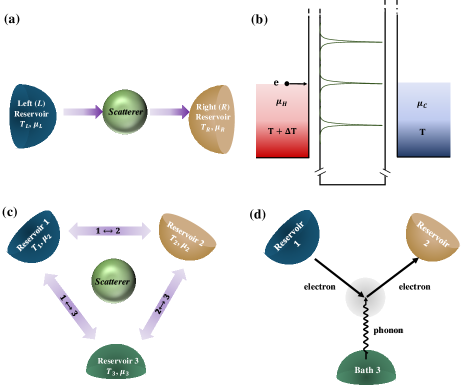
Figure 1: (a) Schematic of Landauer’s theory of transport between two reservoirs. (b) A typical system that can be described by Landauer’s transport theory: resonant tunneling through quantum dots. (c) Büttiker’s theory of decomposing complex transport in multi-terminal systems into many pairs of two-terminal transport processes. (d) An inelastic transport process that cannot be decomposed into pairs of two-terminal transport processes.

Before elaborating on the various surprising properties, we first give an inspirative comparison between thermoelectric engine and solar cells. As shown in Fig. 2(a), a conventional thermoelectric engine consists of two types of semiconductor materials. One of them is $n$-doped, while the other is $p$-doped. Their electrical connection and thermal contact with the heat source and sink are achieved in a bridge like structure in the figure. If this structure is stretched to be straight, as shown in Fig. 2(b), it becomes similar to a solar cell [Fig. 2(c)]. An interesting question arises: why solar cells are more efficient than thermoelectric heat engines, despite that their structures are similar? The key difference between solar cells and thermoelectric heat engines are that they rely on different transport mechanisms. Thermoelectric heat engines rely on diffusive thermoelectric transport in the $p$- and $n$-types of semiconductors which are connected by Ohmic contact via metal electrodes. In contrast, solar cells rely on photo-carrier generation and carrier splitting due to the built-in electric field in the depletion region of the $p$-$n$ junction. While the diffusive thermoelectric transport is based mostly on the elastic transport processes, the photo-carrier generation due to solar radiation is typical inelastic transport processes in semiconductors. Another significant difference is that there are three reservoirs in solar cells, the source, the drain and the Sun. Energy exchange simultaneously takes place among these resoirs. In contrast, there are only two reservoirs in a thermoelectric heat engine. We believe that the much higher energy efficiency in solar cells (typically $>20\%\eta_{C}$ with $\eta_{C}=1-T_{E}/T_{S}$ being the Carnot efficiency of solar cells where $T_{E}$ is the ambient temperature on earth and $T_{S}$ is the black-body radiation temperature of the Sun) Shockley and Queisser (1961); Scully (2010), as compared with the lower energy efficiency of thermoelectric heat engines (typically $<20\%\eta_{C}^{\prime}$ with $\eta_{C}^{\prime}=1-T_{c}/T_{h}$ denoting the Carnot efficiency of thermoelectric heat engines where $T_{c}$ and $T_{h}$ are the temperatures of the cold and hot reservoirs) Jaziri et al. (2020); Tohidi et al. (2022) is not only due to their differences in the Carnot efficiency, $\eta_{C}\gg\eta_{C}^{\prime}$, but also due to the above differences in their transport mechanisms and thermodynamic properties. These differences may also be responsible for the much higher output power in solar cells Jiang et al. (2013a); Jiang and Imry (2017); Wang et al. (2018a). The above thinking inspired us to study inelastic thermoelectric transport in the aim of developing an approach toward high-performance thermoelectric energy conversion beyond the conventional one. In this sense, solar cells are a particular type of inelastic thermoelectric systems that have been put into industrial applications. Solar cells also provide a prototype demonstration on how mesoscopic inelastic thermoelectric systems can be integrated into macroscopic devices. This review is dedicated to the efforts devoted to the emergent field of inelastic thermoelectric effects which seeks for deeper understanding of the underlying physics, generalization of the physical mechanisms, exploration of new effects and new material systems, and investigation of new applications.

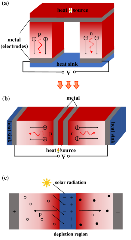
Figure 2: (a) Schematic of the conventional thermoelectric energy harvester that converts heat to electricity. It is composed of two electrically conducting materials: one $n$-type and the other $p$-type. They are joined at the top by a metal (electrode) to make a junction. When the junction is heated, both types of carriers conduct heat to the cold base and a voltage bias is generated at the two base electrodes. (b) The unfolded geometry of the thermoelectric energy harvesting device. (c) Schematic of a solar cell based on a $p$-$n$ junction. Figures (a) and (b) are reproduced from Ref. Li and Jiang (2016).

In the past decade, research on inelastic thermoelectric effects has made notable progresses. There are different types of inelastic thermoelectric systems. For instance, phonon-assisted inelastic thermoelectric systems Jiang et al. (2012, 2013b, 2013a); Jiang and Imry (2016); Jiang et al. (2015a); Jiang and Imry (2017); Agarwalla et al. (2016a, b, 2019), photon-assisted inelastic thermoelectric systems Rutten et al. (2009); Cleuren et al. (2012); Jiang and Imry (2018); Wang et al. (2019a); Houck et al. (2012), magnon-assisted inelastic thermoelectric systems Sothmann et al. (2013), and those systems where inelastic transport is assisted by Coulomb interactions between electrons Sánchez and Büttiker (2011); Sánchez et al. (2013); Sothmann et al. (2012); Whitney et al. (2016); Zhang et al. (2020a, 2017); Mayrhofer et al. (2021). Due to the limited space, we focus in this review phonon- and photon-assisted inelastic thermoelectric effects. In this context, we point out that Coulomb-assisted inelastic thermoelectric systems were reviewed in Ref. Sothmann et al. (2015). At this point, it is necessary to state that to have the inelastic thermoelectric effects well-defined, we need the phonons (or other collective excitations) to have a temperature different from the electrons. This condition often cannot be met in macroscopic systems, therefore we discuss inelastic thermoelectric effects mainly in mesoscopic systems. However, it is possible, via micro fabrication technologies, to integrate these mesoscopic inelastic thermoelectric systems into macroscopic devices. As stated above, solar cells are successful demonstration of such integration.

In this review, we start with a general analysis of thermoelectric transport in mesoscopic systems where elastic and inelastic transport processes are formulated with equal footing. Based on this, we give the bounds on linear transport coefficients for the elastic and inelastic transport processes, respectively. In Sec. IV, we discuss a simple model for phonon-assisted inelastic thermoelectric transport. The unconventional thermoelectric effects induced by the inelastic transport such as rectification, transistor, cooling by heating, and cooling by thermal current effects in the nonlinear regime are considered in Sec. V. Effects that can lead to enhancement of thermoelectric performance, such as the nonlinear transport effect, cooperative effect, and near-field effect are also introduced. The statistics of efficiency for three-terminal systems with (broken) time-reversal symmetry, the thermal transistor amplification factor, and the cooling by heating energy efficiency under the Gaussian fluctuation framework are reviewed in Sec. X. Thermophotovoltaic systems with near-field enhancement are also reviewed as a special category of inelastic thermoelectric systems. Finally, we summarize and give outlooks in Sec. XII.

II Elastic versus inelastic thermoelectric transport in mesoscopic systems

Thermoelectric transport in mesoscopic systems is driven by thermodynamics forces (e.g., temperature gradients and voltage biases). The steady-state transport is characterized by electrical currents and heat currents. The latter consists of contributions from electrons and other quasiparticles such as phonons and photons. Thermoelectric transport can generally be categorized into two main classes: i) elastic transport and ii) inelastic transport Jiang et al. (2015a); Lu et al. (2020).

When a mesoscopic system is connected with two electronic reservoirs, the voltage bias $V$ and the temperature difference $\Delta T=T_{h}-T_{c}$ between the two reservoirs (hot and cold reservoirs, with temperatures $T_{h}>T_{c}$) drive a charge current $I_{e}$ and a heat current $I_{Q}$. In the linear-response regime, the charge and heat currents are related to the thermodynamic affinities (i.e., the voltage bias and the temperature difference) via the Onsager matrix Entin-Wohlman et al. (2014)

$$\left(\begin{array}[]{cccc}I_{e}\\ I_{Q}\end{array}\right)=\left(\begin{array}[]{cccc}G&L\\ L&K\end{array}\right)\left(\begin{array}[]{cccc}V\\ \Delta T/T\end{array}\right),$$ (1)

which is time-reversal symmetry Onsager (1931a, b). $T$ is the average temperature of the system. $G$ and $K$ denote the charge and heat conductivities, respectively. $L$ represents thermoelectric effect and the thermopower (or Seebeck coefficient) is $S=L/(TG)$ Yamamoto et al. (2017). The energy efficiency of the two-terminal thermoelectric system is limited by the second law of thermodynamics Strasberg and Winter (2021). In the linear-response regime the maximum efficiency is given by Harman and Honig (1967); Imry (1997); Chen (2005); Haug and Jauho (2008)

$$\eta_{\rm max}=\eta_{C}\frac{\sqrt{1+ZT}-1}{\sqrt{1+ZT}+1}\leq\eta_{C},$$ (2)

where $\eta_{C}=1-T_{c}/T_{h}$ is the Carnot efficiency. The maximum efficiency show monotonous increase as a function of the dimensionless figure of merit $ZT$, where $ZT=TGS^{2}/K$. Clearly, the maximum efficiency $\eta_{\rm max}$ approaches the Carnot efficiency $\eta_{C}$ when $ZT$ approaches $\infty$. Unfortunately, high values of $ZT$ are difficult to be achieved. In the definition of $ZT$, the heat conductivity $K$ consists of both the electronic heat conductivity and the phononic heat conductivity. In particular, Mahan and Sofo proposed that the “best thermoelectrics” can be realized in narrow-band conductors Mahan and Sofo (1996). Their proposal is based on the arguments that electronic heat conductivity can be suppressed in these narrow-band conductors, while a decent Seebeck coefficient can still be achieved. However, this argument leads to a lot of debates Zhou et al. (2011), and phonon thermal transport will inevitably suppress the figure of merit in these narrow-band conductors. This reveals that there exists intrinsic correlation between the charge and heat transport, since they are both carried by electrons. Though the separation of the charge and heat transport is impossible in elastic transport processes, we will show that it becomes possible in inelastic transport processes.

II.1 The elastic thermoelectric transport: from two-terminal to multiple-terminal setup

Landauer’s scattering theory is an effective description of quantum transport in a two-terminal setup Landauer (1957, 1970); Mazza et al. (2014), as shown in Fig. 1(a). Latter, Büttiker’s multi-terminal version of the scattering theory was placed on a more solid theoretical footing by Ref. Stone and Szafer (1988), which derived it from the Kubo linear-response formalism [see Fig. 1(c)]. The Landauer-Büttiker scattering theory is capable of describing the electrical, thermal, and thermoelectric properties of non-interacting electrons in an arbitrary potential, in terms of the probability that the electrons go from one reservoir to another.

Moreover, the Landauer-Büttiker scattering theory is only applicable to “elastic transport process”, with each microscopic process only involving two reservoirs. Based on the standard Landauer-Büttiker theory Sivan and Imry (1986); Butcher (1990); Benenti et al. (2017), the elastic electronic currents are expressed as

$$I_{e}^{i}|_{\rm el}=\frac{e}{h}\int_{-\infty}^{-\infty}dE\sum_{i\neq j}{\mathcal{T}_{i\rightarrow j}[f_{i}(E)-f_{j}(E)]},$$ (3)

$$I_{Q}^{i}|_{\rm el}=\frac{1}{h}\int_{-\infty}^{-\infty}dE\sum_{i\neq j}{\mathcal{T}_{i\rightarrow j}(E-\mu)[f_{i}(E)-f_{j}(E)]},$$

respectively, where $\mathcal{T}_{ij}$ is the transmission function from reservoir $j$ to reservoir $i$, $f_{i}=\{\exp[(E-\mu_{i})/k_{B}T_{i}]+1\}^{-1}$ is the Fermi-Dirac distribution function, with temperature $T_{i}$ in the ith fermion bath and $\mu_{i}$ the corresponding chemical potential. $k_{B}$ is the Boltzmann constant. Moreover, the probability conservation requires that $\sum_{ij}\mathcal{T}_{i\rightarrow j}=1$ Jiang and Imry (2016). From Eq. (3), it is known that elastic currents are dominated by the two-terminal nonequilibrium processes.

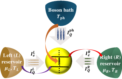
Figure 3: Illustration of possible boson-assisted inelastic transport processes. $I_{e}^{i}$ ($i=L,R$) denoting the electronic current flowing from the $i$th reservoir and $I_{Q}^{i}$ ($i=L,R,{\rm ph}$) denoting the heat current flowing from the $i$th reservoir. Average currents $I_{i}$ are positive when flowing towards the system.

II.2 The inelastic thermoelectric transport assisted by a boson bath

For the three-terminal setup shown in Fig. 3, the electronic (from reservoir $L$ and $R$) and bosonic heat currents (from boson bath) are nonlinearly coupled. Such nonlinearity mainly stems from the inelastic electron-phonon scattering process, which cooperatively involve three reservoirs. This phonon-assisted transport process in the three-terminal nanodevices is termed as “inelastic transport process”. We emphasize that the inelastic transport process in this work is defined for reservoirs (terminals) rather not particles. Therefore, the inelastic transport processes must involve interactions between particles from at least three different terminals. While processes involving only two terminals, although they may involve interactions and energy exchange between quasiparticles, are still elastic transport processes. The inelastic transport process in the present work thus unveils a large number of processes ignored in the conventional study of the mesoscopic transport. It is interesting to note that the inelastic current densities flowing into these terminals are the same. Specifically, the inelastic heat currents flowing into the three reservoirs are expressed via the Fermi golden rule Jiang et al. (2012, 2013b)

$$\begin{aligned} &I_{e}^{L}|_{\rm inel}=-I_{e}^{R}|_{\rm inel}=\iint dE_{1}d\omega_{3}j_{\rm in}(E_{1},\omega_{3}),\\ &I_{Q}^{L}|_{\rm inel}=\iint dE_{1}d\omega_{3}(E_{1}-\mu_{1})j_{\rm in}(E_{1},\omega_{3}),\\ &I_{Q}^{R}|_{\rm inel}=\iint dE_{1}d\omega_{3}(E_{1}-\mu_{2}+\omega_{3})j_{\rm in}(E_{1},\omega_{3}),\\ &I_{Q}^{\rm ph}|_{\rm inel}=\iint dE_{1}d\omega_{3}\omega_{3}j_{\rm in}(E_{1},\omega_{3}),\end{aligned}~{}$$ (4)

where $j_{\rm in}(E_{1},\omega_{3})=C_{\rm in}f_{1}(E_{1})[1-f_{2}(E_{2})]N_{B}(\omega_{3})-C_{in}f_{2}(E_{2})[1-f_{1}(E_{1})][1+N_{B}(\omega_{3})]$, $E_{2}-E_{1}=\omega_{3}$ and $N_{B}(\omega)=[\exp(\omega/k_{B}T_{i})-1]^{-1}$ being the Bose-Einstein distribution function. The transition coefficient $C_{\rm in}$ is the probability for electrons/bosons to tunnel from the $i$th reservoir into the scatterer.

III Bound on the linear transport coefficients for elastic and inelastic transport

Typically, for a scatterer interacting with three reservoirs, we have three corresponding heat currents. However, due to the heat current conservation ($I_{Q}^{L}+I_{Q}^{R}+I_{Q}^{\rm ph}=0$) in the linear-response regime, two of them are independent, e.g., $I_{Q}^{L}$ and $I_{Q}^{\rm ph}$ are two independent heat currents. The transport equation of these heat currents can be expressed as Jiang (2014a)

$$\left(\begin{array}[]{cccc}I_{Q}^{L}\\ I_{Q}^{\rm ph}\end{array}\right)=\left(\begin{array}[]{cccc}K_{11}&K_{12}\\ K_{12}&K_{22}\end{array}\right)\left(\begin{array}[]{cccc}\frac{T_{L}-T_{R}}{T_{R}}\\ \frac{T_{\rm ph}-T_{R}}{T_{R}}\end{array}\right).$$ (5)

$K_{11(22)}$ and $K_{12}$ are the diagonal and off-diagonal thermal conductances, which were originally derived based on the Onsager theory. These two coefficients are obtained by $K_{11}=\partial I_{Q}^{L}/\partial T_{L}$, $K_{12}=\partial I_{Q}^{L}/\partial T_{\rm ph}$, and $K_{22}=\partial I_{Q}^{\rm ph}/\partial T_{\rm ph}$ in the limit $T_{L}$, $T_{R}$, $T_{\rm ph}\rightarrow T$ with $|T_{L({\rm ph})}-T_{R}|\ll T_{R}$.

Then, the bounds of Onsager coefficients based on elastic and inelastic scattering mechanisms can be described, separately. We first consider the generic elastic transport. The elastic coefficients are specified as

$$K^{\rm el}_{ij}=\left\langle E^{2}\right\rangle_{ij}G^{\rm el}_{ij}\quad(i=1,2,3),$$ (6)

where the average under the elastic processes is given by Lu et al. (2017)

$$\left\langle{\mathcal{O}(E)}\right\rangle_{ij}=\frac{\int{dE{\mathcal{O}(E)}G^{\rm el}_{ij}(E)}}{\int{dEG^{\rm el}_{ij}(E)}},$$ (7)

with the probability weight

$$G^{\rm el}_{11}(E) =({\mathcal{T}_{12}}+{\mathcal{T}_{13}})f(E)[1-f(E)],$$ (8a)

$$G^{\rm el}_{12}(E) =(-{\mathcal{T}_{13}})f(E)[1-f(E)],$$ (8b)

$$G^{\rm el}_{22}(E) =({\mathcal{T}_{13}}+{\mathcal{T}_{23}})f(E)[1-f(E)].$$ (8c)

As the transmission probability $\mathcal{T}_{ij}{\geq}0$ is positive, it is straightforward to obtain the boundary of elastic transport coefficients as follows,

$$-1\leq{K^{\rm el}_{12}/K^{\rm el}_{22}}\leq 0,\quad-1\leq{K^{\rm el}_{12}/K^{\rm el}_{11}}\leq 0.$$ (9)

The above expression is presented graphically by the red shadow regime in Fig. 4 .

While for a typical inelastic device consisting of three terminals, the Onsager coefficients are expressed as Mahan and Sofo (1996)

$$K^{\rm inel}_{11}=\left\langle E^{2}_{1}\right\rangle G^{\rm inel}_{11},$$ (10a)

$$K^{\rm inel}_{12}=\left\langle E_{1}\omega_{3}\right\rangle G^{\rm inel}_{12},$$ (10b)

$$K^{\rm inel}_{22}=\left\langle\omega^{2}_{3}\right\rangle G^{\rm inel}_{22}.$$ (10c)

where the ensemble average over all inelastic processes is carried out as

$$\left\langle{\mathcal{Q}(E,\omega)}\right\rangle=\frac{\iint{dEd\omega{\mathcal{Q}(E,\omega)}G^{\rm inel}(E,\omega)}}{\iint{dEd{\omega}G^{\rm inel}(E,\omega)}},$$ (11)

with $G^{\rm inel}=C_{\rm in}f_{1}(E_{1})[1-f_{2}(E_{2})]N_{B}(\omega_{3})$. By applying the Cauchy-Schwarz inequality $\left\langle E^{2}_{1}\right\rangle\left\langle\omega^{2}_{3}\right\rangle-\left\langle E_{1}\omega_{3}\right\rangle^{2}\geq 0$, it is interesting to find that inelastic transport coefficients are bounded by

$$\frac{K^{\rm inel}_{11}}{K^{\rm inel}_{12}}{\times}\frac{K^{\rm inel}_{22}}{K^{\rm inel}_{12}}{\geq}1.$$ (12)

We have provided a generic description of linear electronic and bosonic transport in the three-terminal geometry. Remarkably, the two simple relationships Eqs. (9) and (12) hold for all thermodynamic systems in the linear-response regime.

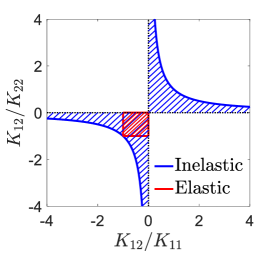
Figure 4: The boundary of the Onsager coefficients. The shaded blue area represents the broadening of the inelastic case, the shaded red area represents the broadening of the elastic case.

IV The basic model of inelastic thermoelectric transport: three-terminal double QD device

A typical inelastic thermoelectric device consists of three terminals: two electrodes (the source and the drain) and a boson bath (e.g., a phonon bath), which is schematically depicted in Fig. 5. In phonon-assisted hopping transport, the figure of merit is limited by the average frequency and bandwidth of the phonons (rather not electrons) involved in the inelastic transport Jiang et al. (2015a). Hartke et al. Hartke et al. (2018) experimentally probes the electron-phonon interaction in a suspended InAs nanowire double QD, which is electric-dipole coupled to a microwave cavity Petersson et al. (2012); Liu et al. (2014); Gullans et al. (2015); Prete et al. (2019); Dorsch et al. (2021); Chen et al. (2017, 2021a).

Specifically, the system is described as the Hamiltonian

$$\hat{H}=\hat{H}_{\rm DQD}+\hat{H}_{\rm e-ph}+\hat{H}_{\rm lead}+\hat{H}_{\rm tun}+\hat{H}_{\rm ph},$$ (13)

with

$$\hat{H}_{\rm DQD} =\sum_{i=\ell,r}E_{i}\hat{c}_{i}^{\dagger}\hat{c}_{i}+(t\hat{c}_{l}^{\dagger}\hat{c}_{r}+{\rm H.c.}),$$ (14a)

$$\hat{H}_{\rm e-ph} =\gamma_{e-{\rm ph}}\hat{c}_{l}^{\dagger}\hat{c}_{r}(\hat{a}+\hat{a}^{\dagger})+{\rm H.c.},$$ (14b)

$$\hat{H}_{\rm ph} =\omega_{0}\hat{a}^{\dagger}\hat{a},$$ (14c)

$$\hat{H}_{\rm lead} =\sum_{j=L,R}\sum_{k}\varepsilon_{j,k}\hat{c}_{j,k}^{\dagger}\hat{c}_{j,k},$$ (14d)

$$\hat{H}_{\rm tun} =\sum_{k}V_{L,k}\hat{c}_{\ell}^{\dagger}\hat{c}_{L,k}+\sum_{k}V_{R,k}\hat{c}_{r}^{\dagger}\hat{c}_{R,k}+{\rm H.c.},$$ (14e)

where $\hat{c}_{i}^{\dagger}$ ($i=\ell,r$) creates an electron in the $i$-th QD with an energy $E_{i}$, $\gamma_{e-{\rm ph}}$ is the strength of electron-phonon interaction, and $\hat{a}^{\dagger}$($\hat{a}$) creates (annihilates) one phonon with the frequency $\omega_{0}$.

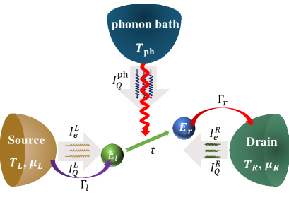
Figure 5: Illustration of three-terminal inelastic transport. An electron left the source into the left QD (with energy $E_{l}$) hops to the right QD (with a different energy $E_{r}$) as assisted by a phonon from the phonon bath (with temperature $T_{\rm ph}$). The electron then tunnels into the drain electrode from the right QD. Such a process gives inelastic charge transfer from the source to the drain assisted by the phonon from the phonon bath. Both the process and its time-reversal contribute to the inelastic thermoelectricity in the system. The electrochemical potential and temperature of the source (drain) are $\mu_{L}$ and $T_{L}$ ($\mu_{R}$ and $T_{R}$), respectively. $t$ is a hopping element between the QDs and $\Gamma_{l/r}$ are the hybridization energies of the dots to the source and drain electrodes, respectively.

For the three-terminal setup in Fig.  5, nonequilibrium steady-state quantities of interest are the electric current $I_{e}$, the electronic heat current traversing from the left reservoir to the right reservoir $I_{Q}^{e}=\frac{1}{2}(I_{Q}^{L}-I_{Q}^{R})$, and the phonon heat current $I_{Q}^{\rm ph}$, with $I_{Q}^{i}$ ($i=L,R,{\rm ph}$) denoting the heat current flowing from the $i$th reservoir. Specifically, the inelastic contribution to the currents is obtained from the Fermi golden rule of Jiang et al. (2012),

$$I_{e}=eI_{N},\,\,\,I_{Q}^{e}=\frac{1}{2}(E_{l}+E_{r})I_{N},\,\,\,I_{Q}^{\rm ph}=(E_{r}-E_{l})I_{N}.$$ (15)

The current factor is $I_{N}=\Gamma_{l\rightarrow r}-\Gamma_{r\rightarrow l}$, and the transition rates are $\Gamma_{l\rightarrow r}\equiv\gamma_{e-{\rm ph}}f_{\ell}(1-f_{r})N_{p}^{-}$ and $\Gamma_{r\rightarrow l}\equiv\gamma_{e-{\rm ph}}f_{r}(1-f_{\ell})N_{p}^{+}$, with $N_{p}^{\pm}=N_{B}+\frac{1}{2}\pm\frac{1}{2}{\rm sgn}(E_{r}-E_{l})$ and the Bose-Einstein distribution for phonons $N_{B}\equiv[\exp({|E_{r}-E_{l}|}/{T_{\rm ph}})-1]^{-1}$.

The thermodynamic affinities conjugated to those three currents satisfy the following relation Onsager (1931a, b)

$${\dot{S}}_{\rm tot}=I_{e}A_{1}+I_{Q}^{e}A_{2}+I_{Q}^{\rm ph}A_{3},$$ (16)

where these conjugated affinities are

$$A_{1} =\frac{\mu_{L}-\mu_{R}}{e}\left(\frac{1}{2T_{L}}+\frac{1}{2T_{R}}\right),\,A_{2}=\frac{1}{T_{R}}-\frac{1}{T_{L}},$$ (17)

$$A_{3} =\frac{1}{2T_{L}}-\frac{1}{2T_{R}}-\frac{1}{T_{\rm ph}}.$$

Hence, based on the the phenomenological transport equations in the linear-response regime, the currents are reexpressed as Jiang et al. (2012); Jiang (2014a, b)

$$\left(\begin{array}[]{cccc}I_{e}\\ I_{Q}^{e}\\ I_{Q}^{\rm ph}\end{array}\right)=\left(\begin{array}[]{cccc}G&L_{1}&L_{2}\\ L_{1}&K_{e}^{0}&L_{3}\\ L_{2}&L_{3}&K_{pe}\end{array}\right)\left(\begin{array}[]{cccc}A_{1}\\ A_{2}\\ A_{3}\end{array}\right),$$ (18)

And two thermopowers are defined as Jiang et al. (2012)

$$S_{1}=\frac{L_{1}}{TG},\quad S_{2}=\frac{L_{2}}{TG}.$$ (19)

In the above Onsager matrix, $G$ denotes the charge conductivity, $L_{1}$ and $L_{2}$ represent the longitudinal and transverse thermoelectric effects Chen et al. (2021b); Zhou et al. (2021), respectively. $K_{e}^{0}$, $K_{pe}$ and $L_{3}$ are the diagonal and off-diagonal thermal conductance, which were originally derived based on the Onsager theory:

$$L_{1}=G\frac{E_{l}+E_{r}}{2e},\quad L_{2}=G\frac{E_{r}-E_{l}}{e},$$ (20)

$$K_{e}^{0}=G\frac{(E_{l}+E_{r})^{2}}{4e^{2}},\quad K_{pe}=G\frac{(E_{r}-E_{r})^{2}}{e^{2}},$$

$$L_{3}=G\frac{(E_{l}+E_{r})(E_{r}-E_{l})}{2e^{2}}.$$

The conductance is $G=\frac{e^{2}}{k_{B}T}\Gamma_{1\rightarrow 2}$, with $\Gamma_{1\rightarrow 2}$ being the inelastic transition rate between the two QDs. We assumed here that the coupling between the left QD and the source as well as that between the right QD the drain is much stronger than the coupling between the two QDs.

V Unconventional thermoelectric effects induced by inelastic transport

In this section, we show that how phonon-assisted inelastic transport leads to unconventional thermoelectric effects, such as the rectification effect, transistor effect, cooling by heating effect, and cooling by thermal current effect.

V.1 Transistors and rectifiers

Diodes and transistors are key components for modern electronics. In recent years, the manipulation and separation of thermal and electrical currents to process information in nano-scale devices have attracted tremendous interests Datta (2005); Bergenfeldt et al. (2014); Sánchez et al. (2017); Guo et al. (2018); Liu et al. (2019); Guo et al. (2019); Wang et al. (2018b); Liu et al. (2022). The design and experimental realization of the thermoelectric device present a striking first step in spin caloritronics, which concerns the coupling of heat, spin, and charge currents in magnetic thin films and other nanostructures Bauer et al. (2012a). Meanwhile, phononic devices, which are devoted to the only use of heat currents for information processing, have also aroused extensive discussions over the past few decades Li et al. (2012).

In Ref. Jiang et al. (2015a), we have shown that thermoelectric rectifier and transistor can be realized in the three-terminal double QD system, in which charge current and electronic and phononic heat currents are inelastically coupled. Specifically, the coupled thermal and electrical transport allows standard rectification, i.e., charge rectification induced by a voltage bias. The magnitudes of the rectification effects are respectively defined by $R_{e}=\frac{I_{e}(V)+I_{e}(-V)}{|I_{e}(V)|+|I_{e}(-V)|}$ for charge rectification, $R_{t}=\frac{I_{Q}^{e}(\delta T)+I_{Q}^{e}(-\delta T)}{|I_{Q}^{e}(\delta T)|+|I_{Q}^{e}(-\delta T)|}$ for electronic heat rectification, $R_{et}=\frac{I_{e}(\delta T)+I_{e}(-\delta T)}{|I_{e}(\delta T)|+|I_{e}(-\delta T)|}$ for charge rectification induced by the temperature difference $\delta T$, and $R_{te}=\frac{I_{Q}^{e}(V)+I_{Q}^{e}(-V)}{|I_{Q}^{e}(V)|+|I_{Q}^{e}(-V)|}$ for heat rectification induced by voltage bias. The results displayed in Fig. 6 including $I_{e}-V$, $I_{Q}^{e}-\delta T$, $I_{Q}^{e}-V$, and the $I_{e}-\delta T$ curves demonstrate significant rectification effects.

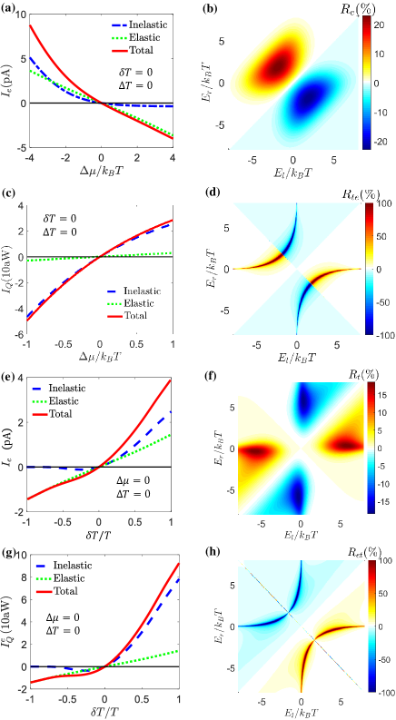
Figure 6: Charge, heat, and cross rectification effects. Figures are reproduced from Ref. Jiang et al. (2015a).

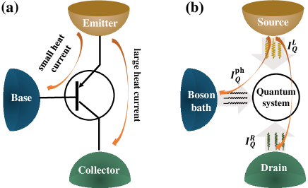
Figure 7: (a) We describe the functioning of a conventional transistor here. A small current flows from emitter to base facilitating a large current from emitter to collector. The ratio of these currents, i.e, $\bar{\alpha}$ is the quantity that characterizes a transistor. (b) The specific three-terminal quantum-dot system that we propose as a transistor is represented here. The source lead, drain lead, and photon bath act like the emitter, collector, and base respectively. The small heat current flowing from the source to the boson bath, $I_{Q}^{\rm ph}$, can control the large heat current flowing from the source to the drain, $I_{Q}^{R}$. The ratio between the two heat currents defines the heat current amplification factor, $\bar{\alpha}$, which characterizes the thermal transistor effect.

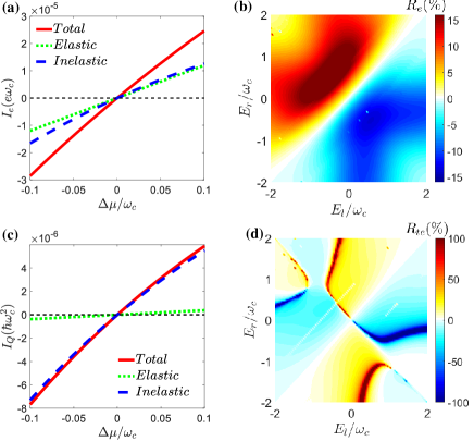
Figure 8: The current (a) and the heat current (c) as the function of $\Delta\mu$. (b) Charge rectification $R_{e}$ and (d) cross rectification $R_{te}$ as the function of $E_{l}$ and $E_{r}$. Figures are reproduced from Ref. Lu et al. (2019a).

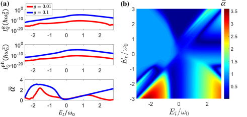
Figure 9: (a) The heat current $I_{Q}^{R}$ flowing out from the right reservoir, photonic heat current $I_{Q}^{\rm ph}$ and heat current amplification factor $\bar{\alpha}$ as function of $E_{l}$ for different electron-photon interaction $g$. (b) The heat current amplification factor $\bar{\alpha}$ as the function of quantum dot energies $E_{l}$ and $E_{r}$. Figures are reproduced from Ref. Lu et al. (2019a).

In addition to the diode effect, we further show that the three-terminal QD system is able to exhibit thermal transistor effect [see Fig.  7]. It has been proposed that negative differential thermal conductance is compulsory for the thermal transistor effect Li et al. (2006, 2012); Liu et al. (2019). Here we remove such restriction on the thermal transistor effect, directly arising from the second law of thermodynamics.

From the phenomenological Onsager transport equation given by Eq. (5), the average heat current amplification factor is then given by

$$\bar{\alpha}=\frac{\partial_{T_{\rm ph}}I_{Q}^{L}}{\partial_{T_{\rm ph}}I_{Q}^{\rm ph}}=\frac{K_{12}}{K_{22}}.~{}$$ (21)

It should be noted that $\overline{\alpha}$ only relies on the general expression of the transport coefficients $K_{12}$ and $K_{22}$. Specifically, for the elastic thermal transport, $\overline{\alpha}_{\rm el}$ is always below the unit as $-1<{K_{12}^{\rm el}}/{K_{22}^{\rm el}}<0$ (red shadow regime in Fig.  4). While for the inelastic case with the constraint coefficients bound at Eq. (12), the average efficiency is given by $\overline{\alpha}_{\rm inel}<\left|{K_{11}^{\rm inel}}/{K_{12}^{\rm inel}}\right|$, which can be modulated in the regime $\overline{\alpha}_{\rm inel}$. Hence, the stochastic transistor may work as ${K_{11}^{\rm inel}}/{K_{12}^{\rm inel}}>1$. Moreover, for the inelastic transport case, the Onsager coefficients are constraint by the second law of thermodynamics, $K_{11}K_{22}-K_{12}^{2}\geq 0$. Therefore, the bound of amplification average efficiency is given by $0<\overline{\alpha}<\infty$ (blue shadow regime in Fig.  4).

A realistic example that achieves $\bar{\alpha}>1$ in the linear-response regime can be found in the three-terminal double QD system Jiang et al. (2015a), which is expressed as

$$\bar{\alpha}=\left|\frac{E_{l}-\mu}{E_{l}-E_{r}}\right|.$$ (22)

When $\left|E_{l}-\mu\right|>\left|E_{l}-E_{r}\right|$, $\bar{\alpha}$ can be greater than unity. Therefore, we conclude that the thermal transistor effect then can also be realized in the linear response regime, in absence of the negative differential thermal conductance.

To further explain those phenomena, we expand the currents up to the second order in affinities

$$I_{i}=\sum_{j}M_{ij}A_{j}+\sum_{jk}L_{ijk}A_{j}A_{k}+{\mathcal{O}}(A^{3}),$$ (23)

where $M_{ij}=M_{ij}^{\rm el}+M_{ij}^{\rm inel}$, with $M_{ij}$ denoting the linear-response coefficients and the second-order terms $L_{ijk}$ only shows up from the inelastic transport processes. Practically, $M_{ij}$ and $L_{ijk}$ can be calculated with realistic material parameters Jiang et al. (2015a). The first term on the right-hand side describes the linear response, whereas the second term gives the lowest-order nonlinear response. The functionalities represented by various second-order coefficients are summarized in Table 1.

The influence of the strong electron-phonon interaction in thermoelectric transport is an intriguing research topic in nonequilibrium transport Burkard et al. (2020); Zhu and Balatsky (2003); Jiang and John (2014); Ren et al. (2012); Mi et al. (2017); Jin et al. (2021); Chen et al. (2022). However, the expression of currents in Eq. ( 15) may break down as the electron-phonon interaction becomes strong, where the high-order electron-phonon scattering processes should be necessarily included to properly characterize the electron current and energy current. Alternatively, the strong light-matter interaction also provides an excellent way for designing efficient thermoelectric devices. In Ref. Lu et al. (2019a), we show that significant rectification effects (including charge and Peltier rectification effects) [see Fig. 8] and linear thermal transistor effects [see Fig. 9] can be enhanced due to the nonlinearity induced by the large electron-photon interaction in circuit-quantum-electrodynamics systems. The above results show that the synergism of electronics and boson in open systems can provide a novel solution for seeking high-performance thermoelectric devices and information storage technology in the future.

Table 1: Functionality of second-order coefficients

Terms ($L_{ijk}$)		Diode or Transistor effect
$L_{111}$		charge rectification
$L_{222}$, $L_{333}$		electronic and phononic heat rectification
$L_{233}$, $L_{322}$		off-diagonal heat rectification
$L_{122}$, $L_{133}$		charge rectification by temperature difference
$L_{211}$, $L_{311}$		heat rectification by voltage bias
$L_{113}$, $L_{123}$		boson-thermoelectric transistor
$L_{212}$, $L_{112}$		other nonlinear thermoelectric effects

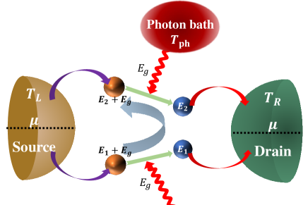
Figure 10: Schematic of the “cooling by heating” refrigerator. The source and drain (with different temperatures $T_{L(R)}$, and electrochemical potentials $\mu_{L}=\mu_{R}\equiv\mu$), are connected by two quantum dots, each having two discrete energy levels.

V.2 Cooling by heating effects

According to Clausius’ second law of thermodynamics, we know that heat cannot spontaneously transfer from the cold reservoir to the hot reservoir Maxwell (1871). Usually, the second law is expressed in a two-terminal system. For three-terminal systems, the second law of thermodynamics has a more complex case where some counterintuitive effects can be allowed Erdman et al. (2018); Bhandari et al. (2018); Friedman and Segal (2019); Manikandan et al. (2020); Liu and Segal (2021). For example, in Ref. Cleuren et al. (2012), Cleuren et al. proposed that one cold reservoir can be cooled by two hot reservoirs without changing the rest of the world due to the transport mechanism of inelastic scattering, which is termed as “cooling by heating” effect.

As exemplified in Fig. 10, to perform cooling by heating a device must have three reservoirs (source, drain, and photon bath) and two adjoining quantum dots. Each quantum dot has a lower and upper energy level. The source is kept at ambient temperature $T_{L}$, photon bath is hotter with $T_{\rm ph}>T_{L}$, and drain is colder with $T_{R}<T_{L}$. The device then utilizes the heat flowing from the photon bath to the source to “drag” heat out of the drain, even though the drain is colder than the other two hot reservoirs.

The basic mechanism is that under the influence of high-temperature photons, the electrons with energy lower than the Fermi level in the source will inelastically pass through the lower energy regime of the two quantum dots and tunnel into the drain. Similarly, the electrons with energy higher than the Fermi level in the drain will transport into the source through the higher energy regime of the two quantum dots. Simultaneously, the electron needs to absorb one photon to complete the cyclic transition process between two quantum dots. The cooling by heating effect in quantum systems can be understood that as the quantum device is driven by the external work, the heat is extracted from the cooling reservoir and absorbed by the hot reservoir.

The efficiency of cooling by heating device (refrigerator) is defined as the heat current flowing out of the drain (the drain being refrigerated) divided by the heat current flowing out of the photon bath, i.e., $\eta_{\rm CBH}={I_{Q}^{R}}/{I_{Q}^{\rm ph}}$. The upper bound on such a refrigerator efficiency is given by the condition that no entropy is generated. Then, the corresponding efficiency is given by

$$\eta^{\rm rev}_{\rm CBH}=\frac{T_{R}(T_{\rm ph}-T_{L})}{T_{\rm ph}(T_{L}-T_{R})}.$$ (24)

Meanwhile, the refrigerator reaches the reversible regime with both heat currents $I_{Q}^{R}$ and $I_{Q}^{\rm ph}$ vanishing simultaneously, while it contains a nonzero cooling efficiency

$$\eta_{\rm CBH}=\frac{E_{2}-E_{1}}{2E_{g}},$$ (25)

with the $E_{1}$ and $E_{2}$ being the energies of the right quantum dot, and $E_{g}$ being the energy gap between the upper (down) levels. It is worth noting that the increase of the entropy rate of the whole system is not negative, and the system satisfies the second law of thermodynamics for the entropy reduction in the source and drain is compensated by the larger entropy increase in the photon bath.

V.3 Cooling by heat current effects

In this section, we show that a nontrivial phonon drag effect, termed by “cooling by heat current” Lu et al. (2021), can emerge in four-terminal QD thermoelectric systems with two electrodes and two phonon baths, shown in Fig.  11. The source (or the drain) can be cooled by passing a thermal current between the two phonon baths, without net heat exchange between the heat baths and the electrodes. This effect, which originates from the inelastic-scattering process, could improve the cooling efficiency and output power due to spatial separation of charge and heat transport Entin-Wohlman et al. (2015); Mazza et al. (2015).

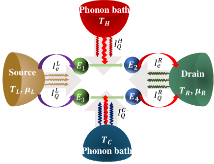
Figure 11: Schematic of quantum dots four-terminal thermoelectric devices. There are two parallel transport channels. Each channel has two quantum dots with different energies and a heat bath to enable inelastic transport. The two channels are spatially separated so that the heat bath $H$ ($C$) couples only to the upper (lower) channel. Four heat currents $I_{Q}^{L}$, $I_{Q}^{R}$, $I_{Q}^{C}$, $I_{Q}^{H}$ and the electric currents $I_{e}$ are illustrated.

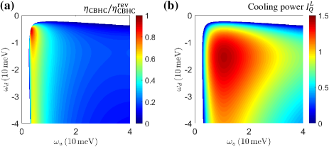
Figure 12: (a) COP and (b) cooling power of the cooling by transverse heat current effect as functions the two energies $\omega_{u}$ and $\omega_{d}$. The white areas represent the parameter regions where the cooling by heat current effect cannot be achieved, i.e., $I_{Q}^{L}<0$. Figures are reproduced from Ref. Lu et al. (2021)

Specifically, the system consists of four quantum dots: QDs 1 and 2 with electronic energy $E_{1}$ and $E_{2}$ are coupled with the hot heat bath $H$, while QDs 3 and 4 with energy $E_{3}$ and $E_{4}$ are coupled with the cold heat bath C. there are one electrical current $I_{e}$ flowing from the source to drain and four heat currents, $I_{Q}^{L}$, $I_{Q}^{R}$, $I_{Q}^{H}$, and $I_{Q}^{C}$. Due to energy conservation Onsager (1931a, b), i.e., $I_{Q}^{L}+\frac{\mu_{L}}{e}I_{e}+I_{Q}^{H}+I_{Q}^{C}+I_{Q}^{R}-\frac{\mu_{R}}{e}I_{e}=0$, the entropy production of the whole system is given by Jiang (2014a)

$$\frac{dS}{dt}=I_{Q}^{L}A_{S}+I_{Q}^{\rm in}A_{\rm in}+I_{Q}^{q}A_{q}+I_{e}A_{e},$$ (26)

and the affinities are defined as

$$A_{S}\equiv\frac{1}{T_{R}}-\frac{1}{T_{L}},\quad A_{\rm in}\equiv\frac{1}{T_{R}}-\frac{1}{2T_{H}}-\frac{1}{2T_{C}},$$ (27)

$$A_{q}\equiv\frac{1}{T_{C}}-\frac{1}{T_{H}},\quad A_{e}\equiv\frac{\mu_{L}-\mu_{D}}{eT_{R}}.$$

$I_{Q}^{\rm in}=I_{Q}^{H}+I_{Q}^{C}$ is regarded as the total heat current injected into the central quantum system from the two thermal baths. $I_{Q}^{q}=(I_{Q}^{H}-I_{Q}^{C})/2$ is the exchanged heat current between the two heat baths intermediated by the central quantum system. $T_{i}$ ($i=L,R,H,C$) are the temperatures of the four reservoirs, respectively. Here, we restrict our discussions on situations where there is only one energy level in each QD that is relevant for the transport.

In this regime, the heat currents derived from the Fermi golden rule Jiang et al. (2015a) can be written as,

$$I_{Q}^{L} =E_{1}I_{12}+E_{3}I_{34},\quad I_{Q}^{H}=\omega_{u}I_{12},\quad I_{Q}^{C}=\omega_{d}I_{34},$$ (28)

$$I_{Q}^{\rm in} =\omega_{u}I_{12}+\omega_{d}I_{34},\quad I_{Q}^{q}=\frac{1}{2}(\omega_{u}I_{12}-\omega_{d}I_{34}).$$

Here $I_{12}=\Gamma_{1\rightarrow 2}-\Gamma_{2\rightarrow 1}$ ($I_{34}=\Gamma_{3\rightarrow 4}-\Gamma_{4\rightarrow 3}$) is the phonon-assisted hopping particle currents through the up (down) channel. $\Gamma_{i\rightarrow j}$ is the electron transfer rate from QD $i$ to QD $j$ Jiang et al. (2012, 2013b), and $\omega_{u}=E_{2}-E_{1}$, $\omega_{d}=E_{4}-E_{3}$ denoting the QDs energy difference in the up and down channel.

We note that the source by driving a heat current between the heat baths $H$ and $C$, i.e., “cooling by heat current effect”, is different from the above “cooling by heating effect” where cooling is driven by a finite heat current injected into the quantum system. In the cooling by heat current effect, heat injected into the quantum system is not necessary, since the driving force of the cooling is the energy exchange between the two heat baths via the central quantum system.

For convenience, we demonstrate the cooling by heat current effect in the situations with $A_{e}=A_{\rm in}=0$. The coefficient of performance (COP) in our four-terminal system can be given by Lu et al. (2019b, 2021)

$$\eta_{\rm CBHC}=\frac{I_{Q}^{L}}{I_{Q}^{q}}.$$ (29)

The reversible COP is $\eta^{\rm rev}_{\rm CBHC}=-{A_{q}}/{A_{S}}$. We show how the cooling power $I_{Q}^{L}$ and COP $\eta_{\rm CBHC}$ vary with the two energies, $\omega_{u}$ and $\omega_{d}$ in Fig. 12. Both the COP $\eta_{\rm CBHC}$ and the cooling power $I_{Q}^{L}$ favor the situations with $-\omega_{u}>\omega_{d}$. For such a regime, cooling induced by the cold terminal $C$ is more effective, for each phonon emission process provides more energy to the heat bath $C$.

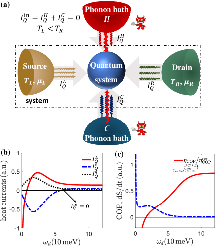
Figure 13: (a) Schematic of a four-terminal mesoscopic thermoelectric device as a Maxwell demon. The demon supplies no work or heat to the system, i.e., the total heat current injected into the central quantum system from the two thermal baths is zero, $I_{Q}^{\rm in}=I_{Q}^{H}+I_{Q}^{C}=0$. (b) Thermal currents, and (c) coefficient of performance ratio $\eta_{\rm CBHC}/\eta^{\rm rev}_{\rm CBHC}$ and entropy production $dS/dt$ as a function of the QD energy $\omega_{d}$. Only when the case with $I_{Q}^{\rm in}=0$ represents that the nonequilibrium Maxwell demon. Figures are reproduced from Ref. Lu et al. (2021).

As shown in Fig. 13, we further find that the cooling by heat current effect can indeed exist when the total heat current injected into the quantum system vanishes (i.e., $I_{Q}^{\rm in}=0$), which termed as “Maxwell demon” Sánchez et al. (2019a, b); Annby-Andersson et al. (2020); Lu et al. (2021); Koski et al. (2014a, 2015, b); Chida et al. (2017); Xi et al. (2021). The Maxwell demon based on two nonequilibrium baths (the cold and hot baths) can reduce the entropy of the system (the source and the drain), without giving energy or changing the particle number of the system. More specifically, the heat current can flow from the cold bath to the hot one without external energies or changing the number of particles in the system.

VI Enhancing three-terminal thermoelectric performance using nonlinear transport effects

Nonlinear transport effects can enhance elastic and inelastic thermoelectric efficiency and power when the voltage and/or temperature bias is large Jiang and Imry (2017). The reason is that linear-response theory usually fails when the voltage and/or temperature bias on the scale of the electrons’ relaxation length (typically given by the electron-electron or electron-phonon scattering length) is comparable to the average temperature. This point is particularly important for many thermoelectric applications. In particular, Sánchez et al. based on the seminal works Sánchez and López (2016); Sánchez and Serra (2011); Sánchez and López (2013); López and Sánchez (2013); Sánchez et al. (2019c), investigated nonlinear quantum transport through nanostructures and mesoscopic systems driven by thermal gradients or in combination with voltage biases. Specifically, when the temperature of the phonon bath increases, the nonlinear thermoelectric transport leads to significant improvement of both the heat-to-work energy efficiency and the output electric power. All these effects are found to be associated with inelastic and elastic thermoelectric contributions.

VI.1 Effects of nonlinear transport on efficiency and power for elastic thermoelectric devices

We study the nonlinear transport effects on the performance of elastic thermoelectric devices. A simple candidate of such devices is a two-terminal QD thermoelectric device, i.e., a QD with energy $E_{0}$ connected with the source (of temperature $T_{h}$) and the drain (of temperature $T_{c}<T_{h}$) electrodes via resonant tunneling Saryal et al. (2021); Liu et al. (2021). The electrical and heat currents can be calculated using the Landauer formula Sivan and Imry (1986); Butcher (1990); Benenti et al. (2017)

$$I_{e}=e\int\frac{dE}{2\pi}{\cal T}_{e}(E)[f_{L}(E)-f_{R}(E)],$$ (30a)

$$I_{Q}^{e}=\int\frac{dE}{2\pi}(E-\mu_{L}){\cal T}_{e}(E)[f_{L}(E)-f_{R}(E)],$$ (30b)

with the energy-dependent transmission function ${\cal T}_{e}(E)=\frac{\gamma_{e}^{2}}{(E-E_{0})^{2}+\gamma_{e}^{2}}$.

Here, we consider harvesting the heat from the hot reservoir to generate electricity. The energy efficiency is hence described as

$$\eta_{\rm HE}=\frac{P_{\rm HE}}{Q_{\rm in}}\leq\eta_{C},$$ (31)

with $T_{h}=T_{\rm ph}$ and $T_{c}=T_{L}=T_{R}$. The output power is

$$P_{\rm HE}=-I_{e}V.$$ (32)

with $\mu_{L}=eV/2=-\mu_{R}$. The heat injected into the system from the hot reservoir is given by

$$Q_{\rm in}=I_{Q}^{e}+I_{Q}^{\rm pr},$$ (33)

with $I_{Q}^{\rm pr}$ being the parasitic phonon heat current Jiang and Imry (2017).

VI.2 Nonlinear transport enhances efficiency and power for inelastic thermoelectric devices

We study the energy efficiency and output power of a double-QDs three-terminal thermoelectric device in the nonlinear transport regime. The device is schematically depicted in Fig.  5. Here, we consider harvesting the heat from the phonon bath to generate electricity. The heat injected into the system from the photon bath is given by

$$Q_{\rm in}=I_{Q}^{\rm ph}+I_{Q}^{\rm pr},$$ (34)

where $I_{Q}^{\rm ph}=2(E_{r}-E_{l})\Gamma_{12}$ is the phononic current flowing from the phonon bath and $\Gamma_{12}$ is the rate of electron transfer from the left QD to the right QD due to the electron-phonon scattering. The electrical current is given by

$$I_{e}=2e\gamma_{e}[f_{L}(E_{l})-f_{1}]+2e\gamma_{e}^{\prime}[f_{L}(E_{r})-f_{2}],$$ (35)

where the factor of two in the above equation comes from electron spin degeneracy. $f_{i}$ ($i=1,2$) are the probabilities of finding an electron on the $i$th QD, and they are determined by the nonequilibrium steady-state distributions on the QDs,

$$0=\frac{df_{1}}{dt}=-\gamma_{e}[f_{1}-f_{L}(E_{l})]-\gamma_{e}^{\prime}[f_{1}-f_{R}(E_{l})]-\Gamma_{12},$$ (36)

$$0=\frac{df_{2}}{dt}=-\gamma_{e}[f_{2}-f_{R}(E_{r})]-\gamma_{e}^{\prime}[f_{2}-f_{L}(E_{r})]+\Gamma_{12}.$$

$\gamma_{e}/\gamma_{e}^{\prime}$ is the tunneling between the QD and the reservoir. The linear transport coefficients are obtained by calculating the ratios between currents and affinities in the regime with very small voltage bias and temperature difference [see Eq. (18)].

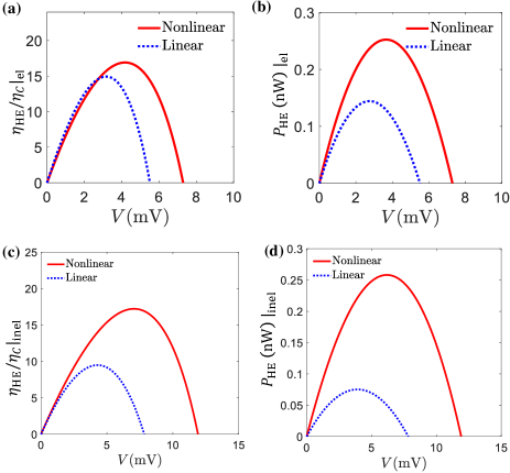
Figure 14: (a)-(b). Elastic thermoelectricity. (a) Energy efficiency $\eta_{\rm HE}/\eta_{C}$ and (b) output power $P_{\rm HE}$ as a function of voltage $V$ (in units of mV) for nonlinear and linear transport. (c)-(d) Inelastic thermoelectricity. (a) Energy efficiency $\eta_{\rm HE}/\eta_{C}$ and (b) output power $P_{\rm HE}$ as functions of voltage $V$ (in units of mV) for the inelastic thermoelectric device. Figures are reproduced from Ref. Jiang and Imry (2017).

In Fig. 14, we perform a comparative study of the nonlinear transport effect on the maximum efficiency and power for inelastic and elastic thermoelectric devices systematically. We find that the nonlinear effect can significantly improve the performance of thermoelectric devices, e.g., thermodynamic efficiency and output power, both for elastic and inelastic cases.

VII Enhancing efficiency and power of three-terminal device by thermoelectric cooperative effects

In the following section, we discuss how the efficiency and output power of the three-terminal heat device can be enhanced by the thermoelectric cooperative effect in the linear-response regime. We consider the setup shown schematically in Fig.  15, which consists of two electronic reservoirs and a phonon bath. The central cavity, which is warmed up by the phonon bath, is connected to two electrodes via two QDs at energy $E_{l(r)}$. There are two thermoelectric effects, one of which belongs to inelastic processes, while the other exists in the elastic process. These two effects are related to two temperature gradients and correspond to the transverse and longitudinal thermoelectric effects, respectively. We show that the energy cooperation between the transverse and longitudinal thermoelectric effects in the three-terminal thermoelectric systems can lead to markedly improved performance of the heat device.

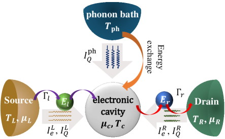
Figure 15: Schematic view of a three-terminal thermoelectric system. The three-terminal device is composed by two electronic reservoirs and a phonon bath, which is held at $T_{\rm ph}$ temperature, The central cavity, which is thermalized by the phonon bath, is connected to two electrodes via two quantum dots at energy $E_{l/(r)}$.

A full description of the thermoelectric transport in three-terminal systems is given by Eq. (18). The cooperative effects in the thermoelectric engine can be elucidated by a geometric interpretation Jiang (2014b); Lu et al. (2017); Liu et al. (2020). The two temperature differences can be parametrized as

$$\delta T=T_{A}\cos\theta,\quad\Delta T=T_{A}\sin\theta.$$ (37)

At given $\theta$, the figure of merit is given by

$$ZT=\frac{GS_{\rm eff}^{2}T^{2}}{K_{\rm eff}-GS_{\rm eff}^{2}T^{2}}.$$ (38)

Here, $S_{\rm eff}=S_{1}\cos\theta+S_{2}\sin\theta$ and $K_{\rm eff}=K_{e}^{0}\cos^{2}\theta+2L_{3}\sin\theta\cos\theta+K_{pe}\sin^{2}\theta$. $S_{1}$ and $S_{2}$ given by Eq. (19) denote the longitudinal and transverse thermopowers, respectively. Then, the “second-law efficiency” of the thermoelectric engine is expressed as

$$\phi=\frac{-I_{e}^{L}V}{I_{Q}^{L}A_{2}+I_{Q}^{\rm ph}A_{3}}\leq\phi_{\max}=\frac{\sqrt{ZT+1}-1}{\sqrt{ZT+1}+1},$$ (39)

which is defined by the output free energy divided by the input free energy Jiang (2014a); Hajiloo et al. (2020); Manzano et al. (2020). The rate of variation of free energy associated with a current is given by the product of the current and its conjugated thermodynamic force. Hence, the denominator of the above equation consists of heat currents multiplied by temperature differences. Such free-energy efficiencies have been discussed for near-equilibrium thermodynamics (in the linear response regime) or arbitrarily far from equilibrium, ranging from biological Caplan (1966) to quantum Hall system Sánchez et al. (2015, 2019b); Gresta et al. (2019); Hajiloo et al. (2020).

Upon optimizing the output power of the thermoelectric engine, one obtains $W_{\max}=\frac{1}{4}P_{F}T_{A}^{2}$, with the power factor

$$P_{F}=GS_{\rm eff}^{2}.$$ (40)

When $\theta=0$ or $\pi$, Eqs. ( 38) and ( 40) give the well-known figure of merit and power factor for the longitudinal thermoelectric effect

$$Z_{l}T=\frac{GS_{1}^{2}T^{2}}{K_{e}^{0}-GS_{1}^{2}T^{2}},\quad P_{Fl}=GS_{1}^{2}.$$ (41)

While the transverse thermoelectric figure of merit and power factor, i.e., $\theta=\pi/2$ or $3\pi/2$, are given by

$$Z_{t}T=\frac{GS_{2}^{2}T^{2}}{K_{pe}-GS_{2}^{2}T^{2}},\quad P_{Ft}=GS_{2}^{2}.$$ (42)

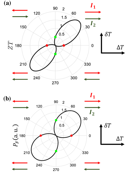
Figure 16: Polar plot of (a) figure of merit $ZT$ and (b) power factor $P_{F}$ [in arbitrary unit (a.u.)] versus angle $\theta$. At $\theta=0^{\circ}$ or $180^{\circ}$ $ZT$ and $P_{F}$ recover the values for the longitudinal thermoelectric effect (red dots), while at $\theta=90^{\circ}$ and $270^{\circ}$ they go back to those of the transverse thermoelectric effect (green squares). The arrows in the I, II, III, IV quadrants label the direction of the currents $I_{1}\equiv L_{1}\Delta T/T$ (red arrows) and $I_{2}\equiv L_{2}\delta T/T$ (green arrows). Figures are reproduced from Ref. Jiang (2014b).

Actually, one can maximize the figure of merit by tuning the angle $\theta$. This is achieved at $\partial_{\theta}(ZT)=0$ and one finds the maximum figure of merit is

$$Z_{m}T=\frac{G(K_{e}^{0}K_{pe}-L_{3}^{2})}{D_{\cal M}}-1.$$ (43)

where $D_{\cal M}=GK_{e}^{0}K_{pe}-GL_{3}^{2}-K_{pe}L_{1}^{2}+2L_{1}L_{2}L_{3}-K_{e}^{0}L_{2}^{2}$ denotes the determinant of the $3\times 3$ transport matrix in Eq.(18). One can also tune $\theta$ to find the maximum power factor

$$P_{Fm}=G(S_{1}^{2}+S_{2}^{2})$$ (44)

is greater than both $P_{Fl}$ and $P_{Ft}$ unless $S_{1}$ or $S_{2}$ is zero.

Fig. 16(a) shows $ZT$ versus the angle $\theta$ in a polar plot for a specific set of transport coefficients. Remarkably for $0<\theta<\pi/2$ and $\pi<\theta<3\pi/2$, $ZT$ is greater than both $Z_{l}T$ and $Z_{t}T$. To understand the underlying physics, we decompose the electric current into three parts $I=I_{0}+I_{1}+I_{2}$ with $I_{0}\equiv GV$, $I_{1}\equiv L_{1}\Delta T/T$, and $I_{2}=L_{2}\delta T/T$. The two thermoelectric effects add up constructively as $I_{1}$ and $I_{2}$ have the same sign, which takes place when $0<\theta<\pi/2$ and $\pi<\theta<3\pi/2$. Fig.  16(b) shows the power factor versus the angle $\theta$. The power factor is also larger when the two currents $I_{1}$ and $I_{2}$ are in the same direction. Therefore, the cooperation of the two thermoelectric effects leads to an enhanced figure of merit and output power.

Besides the multilayer thermoelectric engines, where one electric current is coupled to two temperature gradients, the energy cooperation effects in quantum thermoelectric systems with multiple electric currents and only one heat current have also been studied Lu et al. (2017); Liu et al. (2020), where the elastic tunneling through quantum dots is considered. The constructive cooperation in these quantum thermoelectric systems results in the enhanced thermoelectric power and efficiency for various quantum-dot energies, tunneling rates, etc. Moreover, this cooperative enhancement, dubbed as the thermoelectric cooperative effect, is found to be universal in three-terminal thermoelectric energy harvesting Jordan et al. (2013); Wang et al. (2018a).

VIII Near-field three-terminal thermoelectric heat engine

Near-field thermal radiation recently emerges as one promising route to efficient transfer heat at the nanoscale Zhang (2007); Song et al. (2016); Biehs et al. (2021), which dramatically stimulates the advance of thermoelectics Chen (2005). In Ref. Jiang and Imry (2018), we proposed a near-field thermoelectric heat engine, which is composed of two continuous spectra, e.g., narrow-bandgap semiconductor, separately interacting with single quantum dot and inelastically coupled via the near-field thermal emission. The near-field inelastic heat engine is exhibited to effectively rectify the charge flow of photo-carriers and converts near-field heat radiation into useful electrical power. Such near-field thermoelectric device takes the following advantages of near-field radiations: First, the near-field radiation can strongly enhance heat transfer across the vacuum gap and thus leads to significant heat flux injection. Second, unlike phonon-assisted interband transitions, photon-assisted interband transition is not limited by the small phonon frequency and can work for larger band gaps due to the continuous photon spectrum.

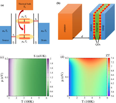
Figure 17: (a) Schematic of near-field three-terminal thermoelectric heat engine. A hot thermal reservoir of temperature $T_{h}$ injects heat flux into the device through near-field heat radiation. The device is held at a lower temperature $T_{c}$. The absorption of the heat radiation is realized by photon-assisted transitions between the two continua. As a result, the upper and lower continua have different chemical potentials, $\mu_{e}$ and $\mu_{v}$, respectively. The source and drain have different electrochemical potentials, denoted as $\mu_{S}$ and $\mu_{D}$, separately. The typical energy of QDs in the left (right) layer is $E_{\ell}$ ($E_{r}$). (b) A possible set-up for the three-terminal near-field heat engine. The emitter is a heat source of temperature $T_{h}$, which is separated from the device by a vacuum gap of thickness $d$. The device is held at a lower temperature $T_{c}$ which consists of the source, drain, and absorber layers. These three parts are divided by two layers of quantum dots arrays. (c) Seebeck coefficient $S$ (in unit of mV/K) and (d) thermoelectric figure of merit $ZT$ for the inelastic thermoelectric transport as functions of the chemical potential $\mu$ and the temperature $T$. Figures are reproduced from Ref. Jiang and Imry (2018).

Here, we present a microscopic theory for the thermoelectric transport in the near-field inelastic heat engine. The Hamiltonian of the system is described as

$$H=H_{\rm SD}+H_{\rm QD}+H_{\rm C}+H_{\rm tun}+H_{\rm e-ph}.$$ (45)

Specifically, the Hamiltonian for the source and drain is expressed as $H_{\rm SD}=\sum_{{\vec{q}}}(E_{S,{\vec{q}}}c^{\dagger}_{S,{\vec{q}}}c_{S,{\vec{q}}}+E_{D,{\vec{q}}}c^{\dagger}_{D,{\vec{q}}}c_{D,{\vec{q}}})$, where ${\vec{q}}$ is the wavevector of electrons. The Hamiltonian of the QDs is $H_{\rm QD}=\sum_{j=\ell,r}E_{j}d^{\dagger}_{j}d_{j}$, where $j=\ell,r$ denotes the left and right dot, respectively. We first consider the case where only one (two if spin degeneracy is included) level in each QD is relevant for the transport. The Hamiltonian for the two central continua is $H_{\rm C}=\sum_{{\vec{q}}}(E_{v,{\vec{q}}}c^{\dagger}_{v,{\vec{q}}}c_{v,{\vec{q}}}+E_{e,{\vec{q}}}c^{\dagger}_{e,{\vec{q}}}c_{e,{\vec{q}}})$. The tunnel coupling through the QDs is given by

$$H_{\rm tun}= \sum_{{\vec{q}}}(J_{S,{\vec{q}}}c_{S,{\vec{q}}}^{\dagger}d_{\ell}+J_{D,{\vec{q}}}c_{D,{\vec{q}}}^{\dagger}d_{r}$$

$$+J_{v,{\vec{q}}}c_{v,{\vec{q}}}^{\dagger}d_{\ell}+J_{e,{\vec{q}}}c_{e,{\vec{q}}}^{\dagger}d_{r})+{\rm H.c.}.$$ (46)

The coupling coefficients $J$ determine the tunnel rates $\Gamma_{ij}$ Jiang and Imry (2018). The Hamiltonian governing the photon-assisted transitions in the center is

$$H_{\rm e-ph}=\sum_{{\vec{q}},{\vec{k}},\tau}\frac{g_{{\vec{k}},\tau}}{\sqrt{V}}c^{\dagger}_{e,{\vec{q}}+{\vec{k}}}c_{v,{\vec{q}}}a_{{\vec{k}},\tau}+{\rm H.c.},$$ (47)

where $g_{\vec{k}}$ is the electron-photon interaction strength, the operator $a_{{\vec{k}},\tau}$ ($\tau=s,p$ denotes the $s$ and $p$ polarized light) annihilates an infrared photon with polarization $\tau$. $V$ is the volume of the photonic system.

Via the Fermi golden rule, the thermoelectric transport coefficients in the linear response regime are obtained as

$$G_{ve}=\frac{e^{2}}{k_{B}T}\int d\omega\Gamma_{0}(\omega),$$ (48a)

$$L_{ve}=\frac{e}{k_{B}T}\int d\omega\Gamma_{0}(\omega)\hbar\omega,$$ (48b)

$$K_{ve}=\frac{1}{k_{B}T}\int d\omega\Gamma_{0}(\omega)\hbar^{2}\omega^{2},$$ (48c)

where

$$\Gamma_{0}(\omega)= 2\pi\nu_{ph}{\cal F}_{nf}(\omega)\sum_{{\vec{q}}}|g(\omega)|^{2}\delta(E_{e,{\vec{q}}}-E_{v,{\vec{q}}}-\hbar\omega)$$

$$\times f^{0}(E_{v,{\vec{q}}},T)[1-f^{0}(E_{e,{\vec{q}}},T)]N^{0}(\omega,T).$$ (49)

The superscript 0 in the above stands for the equilibrium distribution, $N^{0}(\omega_{\vec{k}},T_{c})=1/[\exp(\frac{\hbar\omega_{\vec{k}}}{k_{B}T_{c}})-1]$ is the equilibrium photon distribution function, and $f^{0}(E_{v,{\vec{q}}},T)=1/[\exp(\frac{E_{v,{\vec{q}}}-\mu}{k_{B}T})+1]$ is the Fermi-Dirac distribution function. $|g(\omega)|^{2}=\frac{\hbar\omega d_{cv}^{2}}{2\varepsilon_{0}\varepsilon_{r}}$, $\nu_{ph}$ is the photon density of states, and the factor is given by

$${\cal F}_{nf}(\omega)=\frac{1}{4}\int_{0}^{1}\frac{x_{k}dx_{k}}{\sqrt{1-x_{k}^{2}}}\sum_{\tau}{\cal T}_{\tau}(\omega,x_{k}n\omega/c,d),$$ (50)

where $x_{k}=k_{\parallel}/(n\omega/c)$. It is interesting to show that the photon tunneling probability is specified as Polder and Van Hove (1971); Zhang (2007)

$${\cal T}_{\tau}(\omega_{\vec{k}},k_{\parallel},d)=\left\{\begin{array}[]{cccc}\frac{(1-|r^{\tau}_{01}|^{2})(1-|r^{\tau}_{02}|^{2})}{|1-r^{\tau}_{01}r^{\tau}_{02}e^{i2k^{0}_{z}d}|^{2}},\quad{\rm if}\quad k_{\parallel}\leq\omega/c\\ \frac{4\Im(r^{\tau}_{01})\Im(r^{\tau}_{02})e^{-2\beta^{0}_{z}d}}{|1-r^{\tau}_{01}r^{\tau}_{02}e^{-2\beta^{0}_{z}d}|^{2}},\quad{\rm otherwise}\end{array}\right.$$ (53)

Here $r^{\tau}_{01}$ ($r^{\tau}_{02}$) is the Fresnel reflection coefficient for the interface between the vacuum (denoted as “0”) and the emitter (absorber) [denoted as “1” (“2”)]. $k^{0}_{z}=\sqrt{(\omega/c)^{2}-k_{\parallel}^{2}}$ is the wavevector perpendicular to the planar interfaces in the vacuum. For $k_{\parallel}>\omega/c$, the perpendicular wavevector in the vacuum is imaginary $i\beta^{0}_{z}=i\sqrt{k_{\parallel}^{2}-(\omega/c)^{2}}$, where photon tunneling is dominated by evanescent waves. For isotropic electromagnetic media, the Fresnel coefficients are given by $r^{s}_{0j}=\frac{k_{z}^{0}-k_{z}^{j}}{k_{z}^{0}+k_{z}^{j}}$ and $r^{p}_{0j}=\frac{\varepsilon_{j}k_{z}^{0}-k_{z}^{j}}{\varepsilon_{j}k_{z}^{0}+k_{z}^{j}}~{}(j=1,2)$, where $k_{z}^{j}=\sqrt{\varepsilon_{j}(\omega/c)^{2}-k_{\parallel}^{2}}$ and $\varepsilon_{j}$ ($j=0,1,2$) are the (complex) wavevector along the $z$ direction and the relative permittivity in the vacuum, emitter, and the absorber, respectively.

Consequently, the Seebeck coefficient of the near-field inelastic three-terminal heat engine is obtained as

$$S=\frac{\langle\hbar\omega\rangle}{eT},$$ (54)

and the figure of merit is given by

$$ZT=\frac{\langle\hbar\omega\rangle^{2}}{\alpha\langle\hbar^{2}\omega^{2}\rangle-\langle\hbar\omega\rangle^{2}+\Lambda_{nf}},$$ (55)

where the average is defined as $\langle...\rangle=\frac{\int d\omega\Gamma_{0}(\omega)...}{\int d\omega\Gamma_{0}(\omega)}$, $\alpha={G_{ve}}/{G_{eff}}$, and $\Lambda_{nf}=e^{2}K_{para}/G_{ve}$ characterizes the parasitic heat conductance $K_{para}$ that does not contribute to thermoelectric energy conversion. It is shown in Fig. 17(c) that the Seebeck coefficient does not change significantly by tuning the chemical potential, which is a generic characteristic of the inelastic thermoelectric effect, for the average energy $\langle\hbar\omega\rangle$ is mainly limited by the band gap $E_{g}$ and the temperature $T$. Moreover, the figure of merit with small parasitic heat conduction, e.g, $\Lambda_{nf}=0.2E^{2}_{g}$ in Fig. 17(d), can be optimized as large as $ZT>7$ around $T=350$ K and $\mu>0.15$ eV. Therefore, our work presents one intriguing mechanism of photon-induced inelastic thermoelectricity, which may provide physical insight for future thermoelectric technologies based on inelastic transport mechanisms, and serve as the foundations for future studies.

IX Quantum efficiency bound for continuous heat engines coupled to non-canonical reservoirs

The efficiency of heat engines is fundamentally restricted by the second law of thermodynamics to the Carnot limit Strasberg and Winter (2021). This canonical bound is being challenged nowadays by quantum and classical effects. However, nonequilibrium reservoirs that are characterized by additional parameters besides their temperature are exploited to construct devices with efficiency beyond the Carnot bound Roßnagel et al. (2014a); Klaers et al. (2017).

We study energy conversion in quantum engines absorbing heat from a non-canonical reservoir Agarwalla et al. (2017). The device consists of a single qubit coupled to hot squeezed photon bath and two cold electronic reservoirs (the source and drain), shown in Fig.  18. In order to describe the system quantum mechanically, we apply the two-time measurement protocol to define the characteristic function as

$$\mathcal{Z}(\lambda_{c},\lambda_{e},\lambda_{\rm ph})$$

$$=\langle e^{i\lambda_{c}\hat{A}_{c}+i\lambda_{e}\hat{A}_{e}+i\lambda_{\rm ph}\hat{A}_{\rm ph}}e^{\!-i\lambda_{c}\hat{A}_{c}(t)\!-i\lambda_{e}\hat{A}_{e}(t)\!-i\lambda_{\rm ph}\hat{A}_{\rm ph}(t)}\rangle.$$

$\lambda_{c,e,{\rm ph}}$ are counting parameters for the charge, electronic energy, and photonic energy, respectively. $\hat{A}_{c}$, $\hat{A}_{e}$ and $\hat{A}_{\rm ph}$ are the respective operators: $\hat{A}_{c}$ is the number operator corresponding to the total charge in the $L/R$ electrode, $\hat{A}_{e}$ is the Hamiltonian operator for the $L/R$ electrode and $\hat{A}_{\rm ph}$ is the Hamiltonian operator for the photon bath. $\langle...\rangle$ represents an average with respect to the total initial density matrix, which takes a factorized form with respect to the system ($s$) and ($L$, $R$ and $\rm ph$) reservoirs, $\rho_{T}(0)=\rho_{s}(0)\otimes\rho_{L}\otimes\rho_{R}\otimes\rho_{\rm ph}$. The state of the metal leads is described by a grand canonical distribution, $\rho_{i}=\exp[-\beta_{\rm el}(\hat{H}_{i}-\mu_{i}\hat{N}_{i})]/Z_{i}$, with $Z_{i}={\rm Tr}\Big{[}\exp[-\beta_{\rm el}(\hat{H}_{i}-\mu_{i}\hat{N}_{i})]\Big{]}$ being the partition function, $\beta_{i}=1/k_{B}T_{i}$ being the inverse temperature, and $\mu_{i}$ the chemical potential in the $i$th reservoir, respectively.

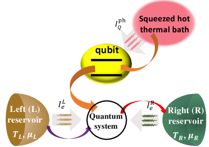
Figure 18: Photoelectric quantum heat engine. Energy absorbed by the qubit from a hot squeezed thermal reservoir is converted to electrical power in the cold electronic system.

IX.1 Equilibrium thermal photon bath

The state of the photon bath is canonical, $\rho_{\rm ph}\!=\!\exp[-\beta_{\rm ph}\hat{H}_{\rm ph}]/Z_{\rm ph}$, with $Z_{\rm ph}={\rm Tr}\big{[}\exp(-\beta_{\rm ph}\hat{H}_{\rm ph})\big{]}$. The fluctuation relation ${\rm ln}\left[P_{t}(\Delta S)/P_{t}(-\Delta S)\right]=\Delta S$ translates to

$$\frac{P_{t}(I_{N},I_{E},I_{Q}^{\rm ph})}{P_{t}(-I_{N},-I_{E},-I_{Q}^{\rm ph})}=e^{\beta_{\rm el}\Delta\mu I_{N}+(\beta_{\rm el}-\beta_{\rm ph})I_{Q}^{\rm ph}}.$$ (56)

Here, $I_{N}$ denotes the number of electrons transferred from $R$ to $L$ during the time interval $t$. Similarly, $I_{E}$ is the electronic energy and $I_{Q}^{\rm ph}$ photonic heat that are exchanged between the baths during the time interval $t$. The characteristics function thus satisfies

$$\mathcal{Z}(\lambda_{c},\lambda_{e},\lambda_{\rm ph})$$ (57)

$$=\mathcal{Z}(-\lambda_{c}+i\beta_{\rm el}(\mu_{R}-\mu_{L}),-\lambda_{e},-\lambda_{\rm ph}-i(\beta_{\rm ph}-\beta_{\rm el}))$$

This relation straightforwardly results in $1=\langle e^{-\beta_{\rm el}\Delta\mu I_{N}+(\beta_{\rm ph}-\beta_{\rm el})I_{Q}^{\rm ph}}\rangle$. Using Jensen’s inequality, we obtain $[-\beta_{\rm el}\Delta\mu\langle I_{N}\rangle+(\beta_{\rm ph}-\beta_{\rm el})\langle I_{Q}^{\rm ph}\rangle]\leq 0$. Therefore, the efficiency, $\langle\eta\rangle\equiv-{\Delta\mu\langle I_{N}\rangle}/{\langle I_{Q}^{\rm ph}\rangle}$, thus obeys the Carnot bound

$$\langle\eta\rangle\leq\frac{\beta_{\rm el}-\beta_{\rm ph}}{\beta_{\rm el}}.$$ (58)

IX.2 Noncanonical photon bath

The squeezed thermal reservoir can be depicted as a combination of orthogonal components, which oscillate as $\cos\omega t$ and $\sin\omega t$ Breuer and Petruccione (2006). Squeezed states have reduced fluctuations in one of the quadratures—but enhanced noise in the other quadrature— to satisfy the bosonic commutation relation. Such states are defined by two parameters, the squeezing factor $r$ and phase Breuer and Petruccione (2006). To restore the detailed balance relation for the $r\neq 0$ case, one can identify an effective temperature Huang et al. (2012)

$$\beta_{\rm eff}=\beta_{\rm ph}+\frac{1}{\hbar\omega_{0}}\ln\left[\frac{1+(1+e^{-\beta_{\rm ph}\hbar\omega_{0}})\sinh^{2}r}{1+(1+e^{\beta_{\rm ph}\hbar\omega_{0}})\sinh^{2}r}\right],$$ (59)

which is unique in the present model, with $\hbar\omega_{0}$ is the energy gap of the qubit.

Identifying the entropy production associated with the photon energy flow by $\langle\Delta S\rangle=(\beta_{\rm el}-\beta_{\rm eff})\langle I_{Q}^{\rm ph}\rangle$, we confirm the symmetry Eq. ( 57) by replacing $\beta_{\rm ph}$ with $\beta_{\rm eff}$

$$\mathcal{Z}(\lambda_{c},\lambda_{e},\lambda_{\rm ph})$$ (60)

$$=\mathcal{Z}(\!-\lambda_{c}\!+i\beta_{\rm el}(\mu_{R}\!-\!\mu_{L}),\!-\lambda_{e},\!-\lambda_{\rm ph}\!-i(\beta_{\rm eff}\!-\beta_{\rm el})).$$

The fluctuation symmetry relation implies that $1=\langle e^{-\beta_{\rm el}\Delta\mu I_{N}+(\beta_{\rm eff}-\beta_{\rm el})I_{Q}^{\rm ph}}\rangle$. Thus, the averaged efficiency, $\langle\eta\rangle\equiv-\Delta\mu\langle I_{N}\rangle/\langle I_{Q}^{\rm ph}\rangle$, is bounded by

$$\langle\eta\rangle\leq 1-\frac{\beta_{\rm eff}}{\beta_{\rm el}}.$$ (61)

We note that this bound is universal, holding even beyond the squeezed-bath case. Explicitly, the efficiency bound for our photoelectric engine Agarwalla et al. (2017) is given by

$$\langle\eta\rangle\leq 1-\frac{\beta_{\rm eff}}{\beta_{\rm el}}+\frac{1}{\beta_{\rm el}\hbar\omega_{0}}\!\ln\left[\frac{1\!+\!(1+e^{\beta_{\rm ph}\hbar\omega_{0}})\sinh^{2}r}{1\!+\!(1+e^{-\beta_{\rm ph}\hbar\omega_{0}})\sinh^{2}r}\right].$$ (62)

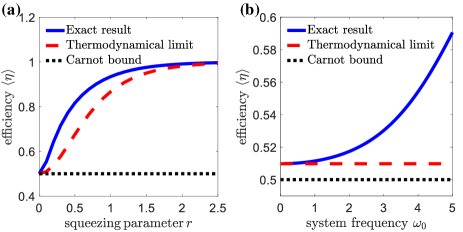
Figure 19: Efficiency bound as a function of (a) squeezing parameter $r$ (b) subsystem frequency $\omega_{0}$. Exact result from Eq. ( 62) (full), thermodynamical limit from Eq. ( 63) (dashed), Carnot bound (dotted). The parameters: $\beta_{\rm el}=2$ and $\beta_{\rm ph}=1$. Figures are reproduced from Ref. Agarwalla et al. (2017).

We now discuss several interesting results of Eq. ( 62). First, we expand it close to thermal equilibrium assuming that $\sinh^{2}r$ is a small parameter. As well, we assume that the temperature of the photon bath is high, e.g., $\beta_{\rm ph}\hbar\omega_{0}\ll 1$. Then, Eq. ( 62) is reduced to

$$\langle\eta\rangle\leq 1-\frac{\beta_{\rm ph}}{\beta_{\rm el}(1+2\sinh^{2}r)}.$$ (63)

which agrees with Ref. Roßnagel et al. (2014b); Manzano et al. (2016). Another interesting case is the deep quantum regime ($\beta_{\rm ph}\hbar\omega_{0}\gg 1$). Assuming small $r$, from Eq. ( 62) we receive an exponential quantum enhancement in comparison to the classical case,

$$\langle\eta\rangle\leq 1-\frac{\beta_{\rm ph}}{\beta_{\rm el}}+\frac{e^{\beta_{\rm ph}\hbar\omega_{0}}}{\beta_{\rm el}\hbar\omega_{0}}\frac{\sinh^{2}r}{1+\sinh^{2}r}.$$ (64)

Fig.  19 clearly exhibits these results: (i) Squeezing enhances the efficiency beyond the Carnot limit. (ii) In the quantum regime ($\beta_{\rm ph}\omega_{0}>1$), the bound is greatly reinforced beyond the thermodynamical limit.

X Thermoelectric efficiency and its statistics

Fluctuations can not be ignored in mesoscopic systems and are particularly important for understanding quantum transport. It can also be considered as a resource for the operations of open quantum systems as functional devices. As a widely used theoretical framework, the fluctuation theorem has been applied to the statistics of the electronic currents, heat currents, and thermodynamic fluctuations Blickle and Bechinger (2012); Seifert (2012); Ciliberto (2017); Seifert (2019); Martínez et al. (2016); Verley et al. (2014a, b); F. and Quan (2018); Agarwalla et al. (2019); Liu and Su (2020); Fei and Quan (2020); Fei et al. (2020); Ma et al. (2020); Fei et al. (2022); Lin et al. (2022). In this section, from the perspective of statistical physics, we will utilize the fluctuation theorem to analyze thermal fractional devices.

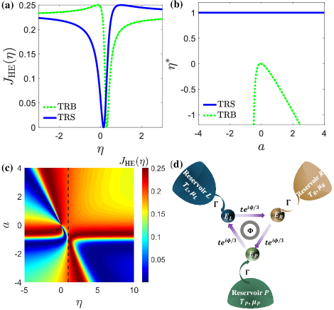
Figure 20: Efficiency statistics for TRS and TRB systems. (a) The LDF $J_{\rm HE}(\eta)$ for TRS and TRB cases as function of $\eta$. (b) The least probable efficiency $\eta^{\star}$ for these two systems at different $a$. (c) LDF $J_{\rm HE}(\eta)$ as a function of $a$ and $\eta$ for a TRB system. (d) A three-terminal triple-QD thermoelectric device with a magnetic flux $\Phi$. Three QD (with $i=1,2,3$) are connected to three electronic reservoirs. The tunneling rates between the QDs and electronic reservoirs is $\Gamma$. Figures are reproduced from Ref. Jiang et al. (2015b).

X.1 Efficiency statistics for three-terminal systems with broken time-reversal symmetry

By analyzing stochastic efficiency, it was recently shown that the Carnot efficiency is the least likely stochastic efficiency Verley et al. (2014b), later found to be solely the consequence of the fluctuation theorem for time-reversal symmetric (TRS) energy transducers Polettini et al. (2015). Breaking the time-reversal symmetry can shift the least likely efficiency away from the Carnot efficiency Gaspard (2013); Polettini et al. (2015).

We consider a generic situation in which there are two energy output channels (“1” and ”2”). Each of the channels has a thermodynamic “current” and a affinity. The time-integrated currents are denoted by $J_{i}$ ($i=1,2$) while the time-intensive current is defined as $I_{i}=J_{i}/t$ with $t$ being the total time of operation. A small time-reverse broken (TRB) machine can be characterized in the linear-response regime by $\overline{{I}}_{i}=M_{ij}A_{j}$ ($i,j=1,2$). In this regime the statistics of the currents at long time $t$ can be described within the Gaussian approximation by the distribution $P_{t}(\vec{I})=\frac{t\sqrt{\det((\hat{M}^{-1})_{sym})}}{4\pi}\exp(-\frac{t}{4}\delta\vec{I}^{T}\cdot\hat{M}^{-1}\cdot\delta\vec{I})$ Andrieux and Gaspard (2004); Proesmans et al. (2016b). Here $\det((\hat{M}^{-1})_{sym})$ is the determinant of the symmetric part of the inverse of the Onsager response matrix $\hat{M}$ and the superscript “$T$” denotes transpose. The averaged quantities are represented with a bar over the symbols throughout this paper. $\delta\vec{I}=\vec{I}-\vec{\overline{{I}}}$ represents fluctuations of the currents. From the probability distribution of stochastic currents we calculate the distribution of efficiency $P_{t}(\eta)$. We then obtain the large deviation function (LDF) of the stochastic efficiency ${\cal G}(\eta)\equiv-\lim_{t\to\infty}t^{-1}\ln[P_{t}(\eta)]$.

Consequently, the scaled LDF ($J(\eta)\equiv{{\cal G}(\eta)}/{\overline{{S}}_{tot}}$) is given by

$$J_{\rm HE}(\eta)=\frac{J_{\rm HE}(\eta_{C})\left(\eta+a^{2}+\alpha qb+aq\eta\right)^{2}}{(1+a^{2}+aqb+aq)\left(\eta^{2}+a^{2}+aq\eta+\alpha qb\eta\right)},$$ (65)

where $\overline{{{S}}}_{tot}=\sum_{i}\overline{{I}}_{i}A_{i}$ is the average total entropy production rate and $J_{\rm HE}(\eta_{C})=\frac{4-q^{2}(1+b)^{2}}{16(1-q^{2}b)}$ is the scaled LDF at Carnot efficiency. Here, $q=\frac{M_{21}}{\sqrt{M_{22}M_{11}}}$, $b=\frac{M_{12}}{M_{21}}$, $a=\frac{A_{1}\sqrt{M_{11}}}{A_{2}\sqrt{M_{22}}}$ are dimensionless parameters that characterize the responses of the system and the applied affinities. In our scheme, efficiency is scaled so that the Carnot (reversible) efficiency corresponds to $\eta_{C}\equiv 1$.

In particular, the minimum $J_{\rm HE}(\bar{\eta}_{\rm HE})=0$ is reached at the average efficiency ${\bar{\eta}}_{\rm HE}=-a(a+qb)/(aq+1)$, whereas the maximum value $J_{\rm HE}(\eta^{\star})=1/4$ is realized at the least probable efficiency

$$\eta^{\star}=1+\frac{q(b-1)(1+aq+aqb+a^{2})}{q-qb-2a+q^{2}(1+b)a}.$$ (66)

In the TRS limit, the least likely efficiency is always identical to the Carnot efficiency, $\eta^{\rm\star}=\eta_{C}\equiv 1$. For TRB systems, in contrast, we find here that $\eta^{\star}$ depends on the parameters $q$, $a$, and $b$, see Figs. 20(a),  20(b), and  20(c).

Moreover, the width of the distribution around the average efficiency, $\sigma_{\eta}^{\rm HE}$, is considered as another key characteristic of efficiency fluctuations. Expanding $J_{\rm HE}(\eta)$ around its minimum $\overline{{\eta}}_{\rm HE}$, one writes $J_{\rm HE}(\eta)\simeq\frac{1}{2(\sigma^{\rm HE}_{\eta})^{2}}(\eta-\overline{{\eta}}_{\rm HE})^{2}+{\cal O}((\eta-\overline{{\eta}}_{\rm HE})^{3})$, to provide here

$$\sigma_{\eta}^{\rm HE}=\frac{2\sqrt{2}|a|(1-q^{2}b)(1+a^{2}+aq+abq)}{(1+aq)^{2}\sqrt{4-q^{2}(1+b)^{2}}}.$$ (67)

We exemplify our analysis within a mesoscopic triple-QD thermoelectric device under a piercing magnetic flux, as shown in Fig.  21.

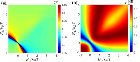
Figure 21: Triple-QD thermoelectric system at maximum average output power condition: (a) Least probable efficiency $\eta^{\star}$, (b) The width of efficiency distribution $\sigma_{\eta}^{\rm HE}$ as functions of QD energies. The white region in (a) depicts very large or very small (negative) $\eta^{\star}$ values which are not properly displayed. Figures are reproduced from Ref. Jiang et al. (2015b).

X.2 Large-deviation function for efficiency: beyond linear-response

In the following, we study the statistics of efficiency fluctuations in the non-equilibrium regime. In a recent study, Esposito et al. analyzed the thermoelectric efficiency statistics in a purely coherent charge transport model Esposito et al. (2015). In parallel, classical models were also examined Verley et al. (2014a). Alternatively, the three-terminal device offers a rich opportunity to examine the thermoelectric efficiency beyond linear response, explore the new concept of efficiency fluctuations, and interrogate the role of quantum effects and many-body interactions on the operation of a molecular thermoelectric engine.

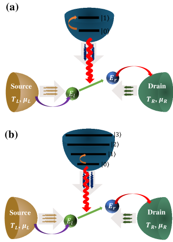
Figure 22: Scheme of a three-terminal QD system. (a) The electron transfer is coupled to a highly anharmonic impurity mode which consists of two QD with $E_{l}$ and $E_{r}$. (b) The vibrational mode is assumed harmonic.

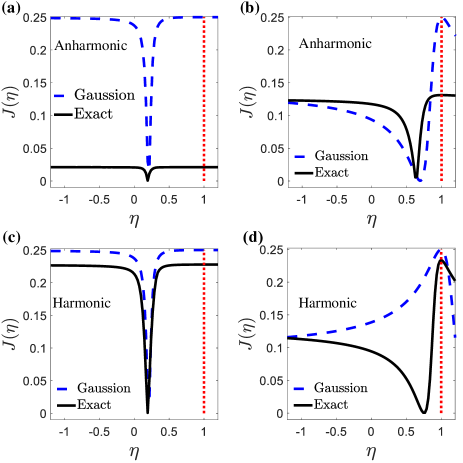
Figure 23: (a) and (b) efficiency LDF $J_{\rm NL}(\eta)$ for the anharmonicity vibrational mode model with different bias voltage (a) $\Delta\mu=0.025\,\rm eV$, (b) $\Delta\mu=0.1\,\rm eV$ for Gaussian limit [Eq. (65)] and exact solution [Eq. (69)]. (c) and (d) efficiency LDF $J_{\rm NL}(\eta)$ for the harmonicity vibrational mode model with different bias voltage (a) $\Delta\mu=0.025\,\rm eV$, (b) $\Delta\mu=0.1\,\rm eV$ for Gaussian limit [Eq. (65)] and exact solution [Eq. (69)]. Figures are reproduced from Ref. Agarwalla et al. (2015a).

Due to the stochastic nature of small systems, efficiency fluctuations are typically not bounded and can take arbitrary values. In general, it is useful to investigate the probability distribution function $P_{t}(\eta)$ to obtain the fluctuating work and heat within the interval $t$, also to observe the value $\eta$ within time $t$. According to the theory of large deviations, the probability function assumes an asymptotic long time form Touchette (2009); Agarwalla et al. (2015b),

$$P_{t}(\eta)\sim e^{-tJ_{\rm NL}(\eta)}$$ (68)

with $J_{\rm NL}(\eta)$ being the “large deviation function”. The large deviation function for efficiency can be obtained from ${\cal G}(\lambda_{w},\lambda_{q})$ by setting $\lambda_{q}=\eta\,\eta_{C}\lambda_{w}$, and minimizing it with respect to $\lambda_{w}$,

$$J_{\rm NL}(\eta)=-\min_{\lambda_{w}}{\cal G}(\lambda_{w},\eta\,\eta_{C}\,\lambda_{w}).$$ (69)

where ${\cal G}(\lambda)$ is the cumulant generating function (CGF) of the three-terminal device. $\lambda_{w}$ and $\lambda_{q}$ are the counting fields for work and heat, respectively. Note that we do not explicitly evaluate the probability distribution function $P_{t}(\eta)$. It can be confirmed that $J_{\rm NL}(\eta)$ has a single minimum, coinciding with the macroscopic efficiency of the engine, and a single maximum, corresponding to the least likely efficiency, which equals to the Carnot efficiency, i.e., $\eta=1$.

We numerically investigate the thermoelectric efficiency and its statistics in the three-terminal device, considering the effects of mode anharmonicity and harmonic vibrational mode beyond linear-response situations. The CGFs for an anharmonic impurity and harmonic vibrational mode models are given by Ref. Agarwalla et al. (2015a). In Fig. 23 we compare the scaled LDF $J(\eta)$ for the two modes in linear-response regime [Eq. (65)] and beyond linear-response regime [Eq. (69)]. It is found that the position $\eta$ for the minimum of $J(\eta)$ can be well captured based on the Gaussian assumption in the linear-response regime. Moreover, such coincidence also persists even at finite thermodynamic bias for the anharmonic case.

X.3 Brownian linear thermal transistors

In Ref. Lu et al. (2020), we have studied the statistical distributions of thermal transistor amplification factor and the cooling by heating efficiency under the assumption of the Gaussian fluctuation. Particularly in the linear-response regime, the statistics of the stochastic heat currents at long time can be described within the Gaussian approximation Gaspard (2013) by the distribution $P_{i}(Q_{L}^{(i)},Q_{\rm ph}^{(i)})=\frac{t\sqrt{\det(\hat{K}^{-1})}}{4\pi}\exp[-\frac{t}{4}\Delta\vec{Q}_{i}^{T}\cdot\hat{K}^{-1}\cdot\Delta\vec{Q}_{i}]$. Here $Q_{L(\rm ph)}^{(1)}=I_{Q}^{L(\rm ph)}(T+\delta T)$ and $Q_{L(\rm ph)}^{(2)}=I_{Q}^{L(\rm ph)}(T_{\rm ph}=T)$ with $\delta T/T\rightarrow 0$. $\Delta\vec{Q}=\vec{Q}-\vec{\overline{Q}}$ represents fluctuations of the heat currents, where $\vec{\overline{Q}}$ is the average heat current and the $\vec{Q}$ is the stochastic one. From the probability distribution of stochastic heat currents, we have the LDF of stochastic thermal transistor Lu et al. (2020)

$$h(\alpha)=\frac{[(K_{12}-K_{22}\alpha)\Delta A_{\rm ph}]^{2}}{8(K_{11}-2K_{12}\alpha+K_{22}\alpha^{2})}.~{}$$ (70)

where $\Delta A_{\rm ph}=A_{\rm ph}^{(1)}-A_{\rm ph}^{(2)}$ and $A_{\rm ph(L)}^{(i)}$ ($i=1,2$) are the affinities for heat currents $Q_{\rm ph(L)}^{(i)}$.

The minimum $h(\bar{\alpha})=0$ locates at the average transistor amplification Jiang et al. (2015a)

$$~{}\overline{\alpha}=\frac{K_{12}}{K_{22}},$$ (71)

which correspond to the maximal probability for the appearance of the amplification efficiency.

The amplification fluctuation is obtained as

$$\sigma_{\alpha}=\frac{2\sqrt{K_{22}(K_{11}K_{22}-K_{12}^{2})}}{K_{22}^{2}\Delta A_{\rm ph}},$$ (72)

which obeys the bound of the Onsager coefficients $K_{11}K_{22}-K_{12}^{2}\geq 0$ and $K_{22}{\geq}0$ Jiang (2014a). The equality is reached as the fluctuation width completely vanishes. Obviously, when this equality is reached, the total entropy production rate of the system in the linear-response regime is $dS/dt\equiv 0$, i.e., the system is in the equilibrium state.

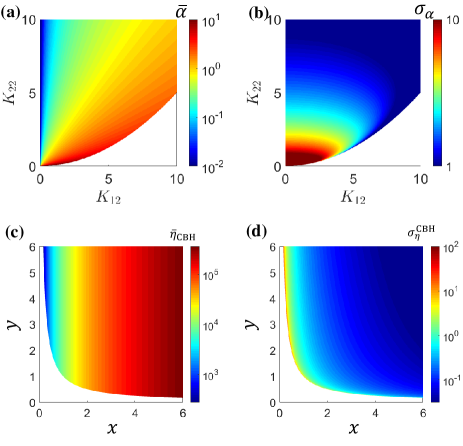
Figure 24: (a) $\bar{\alpha}$ and (b) $\sigma_{\alpha}$ as functions of $K_{12}$ and $K_{22}$. The white region is forbidden by the thermodynamic bound. (c) The average efficiency $\bar{\eta}_{\rm CBH}$ and (d) the width of cooling efficiency distribution $\sigma_{\eta}^{\rm CBH}$. The white region is forbidden by the thermodynamic bound. Figures are reproduced from Ref. Lu et al. (2020).

X.4 The statistics of refrigeration efficiency

Here, we reveal the fluctuations of cooling by heating refrigerators in the linear-response regime. The scaled LDF of stochastic efficiency Verley et al. (2014b); Esposito et al. (2015) can be expressed as

$$g_{\rm CBH}(\eta)=\frac{[1-y\eta+(x-\eta)z]^{2}}{4[x+\eta(-2+y\eta)](xz^{2}+2z+y)},$$ (73)

with dimensionless parameters $x={K_{11}}/{K_{12}}$, $y={K_{22}}/{K_{12}}$, and $z={A_{L}}/{A_{\rm ph}}$. The thermodynamic forces are $A_{L}=(T_{R}-T_{L})/T$ and $A_{\rm ph}=(T_{\rm ph}-T_{L})/T$, respectively.

The minimum of $g_{\rm CBH}(\bar{\eta}_{\rm CBH})=0$ is reached at the average efficiency

$$\bar{\eta}_{\rm CBH}=\frac{xz+1}{y+z}.$$ (74)

The fluctuating width of the average efficiency, $\sigma_{\eta}^{\rm CBH}$, is obtained by expanding $h(\overline{\eta}_{\rm CBH})=0$ around its minimum $\overline{\eta}_{\rm CBH}$,

$$\sigma_{\eta}^{\rm CBH}=\frac{(y+z)^{2}}{(xz^{2}+2z+y)\sqrt{2(xy-1)}}.$$ (75)

Figs. 24(c) and  24(d) illustrate the cooling efficiency $\bar{\eta}_{\rm CBH}$ and the behavior of the width of cooling efficiency distribution $\sigma_{\eta}^{\rm CBH}$ when $z=\infty$. We can observe that the $\sigma_{\eta}^{\rm CBH}$ reaches the maximum under the limit condition, i.e., $(xz+1)(y+z)=0$.

In summary of this section, we emphasize that the statistics of energy efficiency can reveal information on the three-terminal thermoelectric system in the linear and nonlinear regime, and the average efficiency and its fluctuations can further characterize the properties of the system.

XI Thermophotovolatic systems based on near-field tunneling effect

As a solid-state renewable energe resource, thermophotovoltaic (TPV) systems have immense potentials in a wide range of applications including solar energy harvesting and waste heat recovery Liao et al. (2016); Zhao et al. (2017a); Tervo et al. (2018). In the TPV system, a photovoltaic (PV) cell is placed in the proximity of a thermal emitter and converts the thermal radiation from the emitter into electricity via infrared photoelectric conversion. However, the TPV performance is significantly reduced due to the frequency mismatch between the thermal emitter and the PV cell in the TPV systems at moderate temperatures (i.e., 400$\sim$900 K which is the majority spectrum of the industry waste heat). To overcome this obstacle, materials which support surface polaritons have been used to introduce a resonant near-field energy exchange between the emitter and the absorber Ilic et al. (2012); Svetovoy and Palasantzas (2014); Zhao et al. (2017a). As a consequence, near-field TPV (NTPV) systems have been proposed to achieve appealing energy efficiency and output power Laroche et al. (2006); Molesky and Jacob (2015). Near-field systems based on graphene, hexagonal-boron-nitride (h-BN) and their heterostructures have been shown to demonstrate excellent near-field couplings due to surface plasmon polaritons (SPPs), surface phonon polaritons (SPhPs) and their hybridizations [i.e., surface plasmon-phonon polaritons (SPPPs)] Svetovoy et al. (2012); Messina and Ben-Abdallah (2013); Zhao and Zhang (2015); Zhao et al. (2017b); Shi et al. (2017). In Ref. Wang et al. (2019b), we propose to use graphene-h-BN heterostructures Brar et al. (2014); Kumar et al. (2015); Zhao and Zhang (2015); Zhao et al. (2017b); Shi et al. (2017) as the emitter and the graphene-covered InSb $p$-$n$ junction as the TPV cell. We find that such a design leads to significantly improved performance as compared to the existing studies Messina and Ben-Abdallah (2013); Heavens (1991); Knittl (1976).

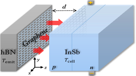
Figure 25:  Schematic representation of the near-field thermophotovoltaic system. A thermal emitter of temperature $T_{\rm emit}$ made of h-BN/graphene heterostructure is placed in the proximity of a thermophotovoltaic cell of temperature $T_{\rm cell}$ made of InSb. The emitter-cell distance is kept at $d$. The red arrows represents the heat flux radiated from the emitter to the cell. The coordinate axes on the left side shows the in-plane (parallel to the $x$-$y$ plane) and out-of plane (perpendicular to the $x$-$y$ plane) directions. Figures are reproduced from Ref. Wang et al. (2019b).

Fig.  25 presents the proposed NTPV system. The emitter is a graphene covered h-BN film of thickness $h$, kept at temperature $T_{\rm emit}$. The TPV cell is made of an InSb $p$-$n$ junction, kept at temperature $T_{\rm cell}$, which is also covered by a layer of graphene. The thermal radiation from the emitter is absorbed by the cell and then converted into electricity via photoelectric conversion. The performance of the NTPV system is characterized by the output electric power density $P_{\rm e}$ and energy efficiency $\eta$.

The output electric power density $P_{\rm e}$ of the NTPV system is defined as the product of the net electric current density $I^{\rm NTPV}_{\rm e}$ and the voltage bias $V$ Wang et al. (2019b),

$$P_{\rm e}^{\rm NTPV}=-I^{\rm NTPV}_{\rm e}V,$$ (76)

and the energy efficiency $\eta^{\rm NTPV}$ is given by the ratio between the output electric power density $P^{\rm NTPV}_{\rm e}$ and incident radiative heat flux $Q_{\rm inc}$,

$$\eta^{\rm NTPV}=\frac{P_{\rm e}^{\rm NTPV}}{Q_{\rm inc}},$$ (77)

The incident radiative heat flux is given by

$$Q_{\rm rad}=Q_{\omega<\omega_{\rm gap}}+Q_{\omega\geq\omega_{\rm gap}}$$ (78)

where $Q_{\omega<\omega_{\rm gap}}$ and $Q_{\omega\geq\omega_{\rm gap}}$ are the heat exchanges below and above the band gap of the cell, respectively Polder and Van H. (1971); Pendry (1999).

The electric current density of a NTPV cell is calculated via the detailed balance analysis Shockley and Queisser (1961),

$$I=I_{\rm ph}-I_{0}[\exp(V/V_{\rm cell})-1],$$ (79)

Where $V_{\rm cell}=k_{\rm B}T_{\rm cell}/e$ is a voltage which measures the temperature of the cell Shockley and Queisser (1961). $I_{\rm ph}$ and $I_{0}$ are the photo-generation current density and reverse saturation current density, respectively. The reverse saturation current density is determined by the diffusion of minority carriers in the InSb $p$-$n$ junction and the photo-generation current density $I_{\rm ph}$ is contributed from the above-gap thermal heat exchange Wang et al. (2019b).

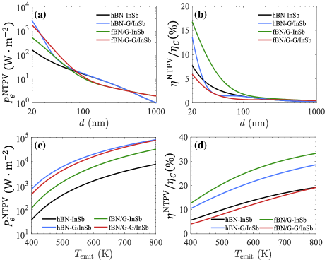
Figure 26: Optimal performances of the four NTPV devices. (a) and (b), Optimal (a) output power density $P^{\rm NTPV}_{\rm e}$ and (b) energy efficiency in unit of the Carnot efficiency ($\eta^{\rm NTPV}/\eta_{\rm C}$) as functions of the vacuum gap $d$. The temperatures of the emitter and the cell are set as $T_{\rm emit}=450$ K and $T_{\rm cell}=320$ K, respectively. (c) and (d), Optimal (c) output power density $P^{\rm NTPV}_{\rm e}$ and (d) energy efficiency in unit of the Carnot efficiency ($\eta^{\rm NTPV}/\eta_{\rm C}$) as functions of the emitter temperature $T_{\rm emit}$ with $d=20$ nm and $T_{\rm cell}=320$ K. For all these figures, the chemical potential of graphene is set as $\mu_{\rm g}=1.0$ eV. The chemical potential difference across the InSb $p$-$n$ junction $\Delta\mu$ is optimized independently for each configuration. Figures are reproduced from Ref. Wang et al. (2019b)

The performances of four different NTPV configurations are examined: (i) the $h$-BN-InSb device (denoted as hBN-InSb, with the mono-structure bulk $h$-BN being the emitter and the uncovered InSb $p$-$n$ junction being the cell), (ii) the $h$-BN-graphene/InSb device (denoted as hBN-G/InSb, with the bulk $h$-BN being the emitter and the graphene-covered InSb $p$-$n$ junction as the cell), (iii) the $h$-BN/graphene-InSb device (denoted as fBN/G-InSb, with the $h$-BN/graphene heterostructure film being the emitter and the uncovered InSb $p$-$n$ junction as the cell), and (iv) the $h$-BN/graphene-graphene/InSb device (denoted as fBN/G-G/InSb, with the $h$-BN/graphene heterostructure film being the emitter and the graphene-covered InSb $p$-$n$ junction as the cell). We study and compare their performances for various conditions to optimize the performance of the NTPV system. As shown in Fig. 26, the primitive hBN-InSb set-up has poor energy efficiency and output power.

The overall best performance comes from the $h$BN-G/InSb (if high output power is preferred) and the fBN/G-InSb (if high energy efficiency is preferred) set-ups. The underlying physics for the different characteristics of the four different set-ups is understood as due to the resonant coupling between the emitter and the $p$-$n$ junction, where the SPPs in graphene and SPhPs in $h$-BN play crucial roles Wang et al. (2019b); Zhao and Zhang (2015); Zhao et al. (2017b); Shi et al. (2017).

Since the semiconductor thin-films have been explored in NTPV systems, we further investigate the performance of the NTPV systems based on thin-film $p$-$n$ junctions. A NTPV system based on a InAs thin-film cell with appealing performance operating at high temperatures has been recently proposed  Zhao et al. (2017a); Papadakis et al. (2020). But the system suffers from low energy efficiency (below $10\%$) when operating at moderate temperature due to the parasitic heat transfer induced by the phonon-polaritons of InAs. In Ref. Wang et al. (2021a), we use InSb as the near-field absorber since the bandgap energy of InSb is lower compared to InAs and its photon-phonon interaction is much weaker than InAs. In this work, we examine the performances of two NTPV devices: the graphene-$h$-BN-graphene-InSb cell (denoted as G-FBN-G-InSb cell, with the graphene-$h$-BN-graphene sandwich structure being the emitter and the InSb thin-film being the cell) and the graphene-$h$-BN-graphene-$h$-BN-InSb cell (denoted as G-FBN-G-FBN-InSb cell, with the double graphene-$h$-BN heterostructure being the emitter and the InSb thin-film being the cell). It is found that the G-FBN-G-InSb cell, despite having a simpler structure, performs better than the G-FBN-G-FBN-InSb cell. While both of the NTPV systems based on InSb thin-film cell underperform the ones based on bulk InSb cell. This is due to the exponential decay characteristic of the electromagnetic wave propagating in the InSb thin-film, which induces an actual availability of the above-gap photons in the photon-carrier generation process Wang et al. (2021a). In general, those devices are promising for heat-to-electricity energy conversion in the common industry waste heat regime.

XII Summary and outlooks

This paper attempts to provide a succinct review of the research frontier of inelastic thermoelectric effects. We summarized both theoretical and experimental progresses on inelastic thermoelectric transport and fluctuation in mesoscopic systems. We first give a general theoretical framework of the thermoelectric elastic and inelastic transport and revealed the unique role of the inelastic process of thermal transport in mesoscopic systems. We then show the distinct bounds on the linear transport coefficients of the elastic and inelastic thermoelectric transport from the general theoretical framework. We further summarize the unprecedented phenomena emerging from inelastic thermoelectric transport such as linear thermal transistor, cooling by heating, heat-charge cross rectification, and cooling by thermal current. Inspired or based on inelastic thermoelectric effects, several approaches to improve thermoelectric performance are summarized, including heat-charge separation, thermoelectric cooperative effects, nonlinear enhancement of performance, non-canonical reservoirs, and near-field enhancement effect. For the near-field enhanced thermoelectric energy conversion, we discuss a set of examples including quantum-dots systems and graphene-h-BN-InSb systems.

Moreover, by integrating spin thermoelectric effect with the concepts from magnonics, the electron-magnon interactions for the nonequilibrium transport has been studied recently in many theoretical Tulapurkar and Suzuki (2010); Bauer et al. (2012b); Chumak et al. (2015); Rezende et al. (2016); Qaiumzadeh et al. (2018); Tang et al. (2018); Upadhyay et al. (2021); Wang et al. (2022a) and experimental works Uchida et al. (2008); Jaworski et al. (2010); Slachter et al. (2010); Walter et al. (2011). The asymmetric spin Seebeck effect, has recently been discovered both in metal/insulating magnet interfaces and magnon tunneling junctions, which leads to many interesting effects, such as spin thermal rectifiers effect Ren and Zhu (2013a), spin transistor effects Ren and Zhu (2013b), logic gates, and negative differential spin Seebeck effects Ren (2013). These properties could have various implications in flexible thermal and spin information control. The generalization of the nanoscale metal-magnetic insulator interfaces with the electron-magnon interactions for inelastic thermoelectric transport and fluctuations in mesoscopic system is an interesting future direction.

In addition to these contents reviewed above, there are still many interdisciplinary research frontiers of great curiosity, which are partially listed below:

(i) Thermodynamic uncertainty relation. Recently, a thermodynamic uncertainty relation has been formulated for classical Markovian systems demonstrating trade-off between current fluctuation (precision) and dissipation (cost) in nonequilibrium steady state Barato and Seifert (2015); Hasegawa (2021); Liu and Segal (2019); Horowitz and Gingrich (2020); Yan et al. (2022). The thermodynamic uncertainty relation implies that a precise thermodynamic process with little noise needs the high entropy production. It is believed to be important in exploring the thermodynamic uncertainty bounds on the multi-terminal inelastic thermoelectric heat engine.

(ii) Geometric-phase-induced pump. The second law of thermodynamics indicates that heat cannot be transferred spontaneously from low-temperature heat reservoir to high-temperature heat reservoir. To go beyond this conventional thermoelectric energy conversion, a Berry-phase-like effect provides an additional geometric contribution Sinitsyn and Nemenman (2007a, b); Ren et al. (2010); Wang et al. (2017, 2022b, 2021b); Terrén Alonso et al. (2022); Lu et al. (2022) to pump electric and heat currents against the thermodynamic bias. Hence, it is intriguing to analyze the influence of the geometric-phase-induced pump in the periodically driven quantum thermal machines Bhandari et al. (2020), e.g., the inelastic thermoelectric engine.

(iii) Enhancing performance of NTPV systems via twisted bilayer two-dimensional materials. The performance of NTPV systems can be greatly improved due to the hybridization effect of polaritons. Recently, the concept of photonic magic angles has attracted the attention of many researchers, due to the manipulation of the photonic dispersion of phonon polaritons in van der Waals bilayers Hu et al. (2020). The twisted two-dimensional bilayer anisotropy materials or insulator slabs are explored in the near-field systems and the near-field radiative heat transfer can be significantly enhanced by the twist-nonresonant surface polaritons He et al. (2020); Tang et al. (2021); Peng et al. (2021). Inspired by this concept, it is extraordinarily promising to enhance the output power and energy efficiency of the NTPV systems by employing the twisted bilayer two-dimensional materials: the near-field absorber and emitter can be consisted of two dimensional anisotropic material/structure, e.g., Van der Waals materials or grating structures.

(iv) Angular momentum radiation. The spin-orbit interaction, i.e., the coupling between the electron (light) orbital motion and the corresponding spin, is fundamentally important in spintronics Awschalom and Samarth (2009), topological physics Hasan and Kane (2010); Qi and Zhang (2011), and nano-optics Bliokh et al. (2015); B. and N. (2015). Recently, the concept of angular momentum radiation was proposed via the spin-orbital interaction in the molecular junctions interacting with the electromagnetic waves Zhang et al. (2020b). Based on the nonequilibrium Green’s function method, the angular momentum selection rule for inelastic transport was unraveled. Hence, it should be interesting in incorporating the angular momentum selection rule into the photon-involved inelastic thermoelectric machines.

XIII Disclosure statement

No potential conflict of interest was reported by the authors.

XIV Funding

This work was supported by the support from the funding for Distinguished Young Scienctist from the National Natural Science Foundation of China (Grant Nos. 12125504, 12074281, 12047541, 12074279, and 11704093), the Major Program of Natural Science Research of Jiangsu Higher Education Institutions (Grant No. 18KJA140003), the Jiangsu specially appointed professor funding, the Academic Program Development of Jiangsu Higher Education (PAPD), the Opening Project of Shanghai Key Laboratory of Special Artificial Microstructure Materials and Technology, the China Postdoctoral Science Foundation (Grant No. 2020M681376), the faculty start-up funding of Suzhou University of Science and Technology, and Jiangsu Key Disciplines of the Fourteenth Five-Year Plan (Grant No. 2021135).

References

- Harman and Honig (1967) T. C. Harman and J. M. Honig, Thermoelectric and thermomagnetic effects and applications (McGraw-Hill, NewYork, 1967).
- Imry (1997) Y. Imry, Introduction to Mesoscopic Physics (Oxford University Press, London, 1997).
- Brandner (2020) K. Brandner, “Coherent transport in periodically driven mesoscopic conductors: From scattering amplitudes to quantum thermodynamics,” Zeitschrift für Naturforschung A 75, 483–500 (2020).
- Brandner et al. (2017) K. Brandner, M. Bauer, and U. Seifert, “Universal coherence-induced power losses of quantum heat engines in linear response,” Phys. Rev. Lett. 119, 170602 (2017).
- Sánchez et al. (2021) R. Sánchez, C. Gorini, and G. Fleury, “Extrinsic thermoelectric response of coherent conductors,” Phys. Rev. B 104, 115430 (2021).
- Potanina et al. (2021) E. Potanina, C. Flindt, M. Moskalets, and K. Brandner, “Thermodynamic bounds on coherent transport in periodically driven conductors,” Phys. Rev. X 11, 021013 (2021).
- Leggett et al. (1987) A. J. Leggett, S. Chakravarty, A. T. Dorsey, Matthew P. A. Fisher, Anupam Garg, and W. Zwerger, “Dynamics of the dissipative two-state system,” Rev. Mod. Phys. 59, 1–85 (1987).
- Proesmans et al. (2016a) K. Proesmans, B. Cleuren, and C. Van den Broeck, “Power-efficiency-dissipation relations in linear thermodynamics,” Phys. Rev. Lett. 116, 220601 (2016a).
- Onsager (1931a) L. Onsager, “Reciprocal relations in irreversible processes. i.” Phys. Rev. 37, 405–426 (1931a).
- Onsager (1931b) L. Onsager, “Reciprocal relations in irreversible processes. ii.” Phys. Rev. 38, 2265–2279 (1931b).
- Callen (1948) H. B. Callen, “The application of onsager’s reciprocal relations to thermoelectric, thermomagnetic, and galvanomagnetic effects,” Phys. Rev. 73, 1349–1358 (1948).
- Saito et al. (2011) K. Saito, G. Benenti, G. Casati, and T. Prosen, “Thermopower with broken time-reversal symmetry,” Phys. Rev. B 84, 201306 (2011).
- Benenti et al. (2011) G. Benenti, K. Saito, and G. Casati, “Thermodynamic bounds on efficiency for systems with broken time-reversal symmetry,” Phys. Rev. Lett. 106, 230602 (2011).
- Jiang (2014a) J.-H. Jiang, “Thermodynamic bounds and general properties of optimal efficiency and power in linear responses,” Phys. Rev. E 90, 042126 (2014a).
- Haug and Jauho (2008) H. Haug and A. P. Jauho, Quantum Kinetics in Transport and Optics of Semiconductors (Springer-Verlag Berlin Heidelberg, 2008).
- Buttiker (1988) M. Buttiker, “Coherent and sequential tunneling in series barriers,” IBM J. Res. Dev. 32, 63–75 (1988).
- Büttiker (1986) M. Büttiker, “Four-terminal phase-coherent conductance,” Phys. Rev. Lett. 57, 1761–1764 (1986).
- Büttiker (1987) M Büttiker, “Transport as a consequence of state-dependent diffusion,” Z. Phys. B 68, 161–167 (1987).
- Meir and Wingreen (1992) Y. Meir and N. S. Wingreen, “Landauer formula for the current through an interacting electron region,” Phys. Rev. Lett. 68, 2512–2515 (1992).
- Jauho et al. (1994) A.-P. Jauho, N. S. Wingreen, and Y. Meir, “Time-dependent transport in interacting and noninteracting resonant-tunneling systems,” Phys. Rev. B 50, 5528–5544 (1994).
- Blanter and Büttiker (2000) Y. M. Blanter and M. Büttiker, “Shot noise in mesoscopic conductors,” Phys. Rep. 336, 1 (2000).
- Wang et al. (2006) J.-S. Wang, J. Wang, and N. Zeng, “Nonequilibrium green’s function approach to mesoscopic thermal transport,” Phys. Rev. B 74, 033408 (2006).
- Lü and Wang (2007) J. T. Lü and J.-S. Wang, “Coupled electron and phonon transport in one-dimensional atomic junctions,” Phys. Rev. B 76, 165418 (2007).
- Wang et al. (2008) J-S Wang, J. Wang, and J. T. Lü, “Quantum thermal transport in nanostructures,” Eur. Phys. J. B 62, 381–404 (2008).
- Wang et al. (2014) J.-S. Wang, B. K. Agarwalla, H. Li, and J. Thingna, “Nonequilibrium green’s function method for quantum thermal transport,” Front. Phys. 9, 673–697 (2014).
- Lü et al. (2016) J.-T. Lü, J.-S. Wang, P. Hedegård, and M. Brandbyge, “Electron and phonon drag in thermoelectric transport through coherent molecular conductors,” Phys. Rev. B 93, 205404 (2016).
- Zhang and Lü (2017) Z.-Q. Zhang and J.-T. Lü, “Thermal transport through a spin-phonon interacting junction: A nonequilibrium green’s function method study,” Phys. Rev. B 96, 125432 (2017).
- Brandner et al. (2018a) K. Brandner, T. Hanazato, and K. Saito, “Thermodynamic bounds on precision in ballistic multiterminal transport,” Phys. Rev. Lett. 120, 090601 (2018a).
- Brandner et al. (2018b) K. Brandner, T. Hanazato, and K. Saito, “Thermodynamic bounds on precision in ballistic multiterminal transport,” Phys. Rev. Lett. 120, 090601 (2018b).
- Tu (2021) Z.-C. Tu, “Abstract models for heat engines,” Front. Phys. 16, 1–12 (2021).
- Carrega et al. (2022) M. Carrega, L. M. Cangemi, G. De Filippis, V. Cataudella, G. Benenti, and M. Sassetti, “Engineering dynamical couplings for quantum thermodynamic tasks,” PRX Quantum 3, 010323 (2022).
- Guo et al. (2016) J. Guo, J.-T. Lü, Y. Feng, J. Chen, J. Peng, Z. Lin, X. Meng, Z. Wang, X.-Z. Li, E.-G. Wang, and J. Yang, “Nuclear quantum effects of hydrogen bonds probed by tip-enhanced inelastic electron tunneling,” Science 352, 321–325 (2016).
- Sothmann et al. (2015) B. Sothmann, R. Sánchez, and A. N Jordan, “Thermoelectric energy harvesting with quantum dots,” Nanotechnology 26, 032001 (2015).
- Jiang and Imry (2016) J.-H. Jiang and Y. Imry, “Linear and nonlinear mesoscopic thermoelectric transport with coupling with heat baths,” C. R. Phys. 17, 1047 – 1059 (2016).
- Thierschmann et al. (2016) H. Thierschmann, R. Sánchez, B. Sothmann, H. Buhmann, and L. W. Molenkamp, “Thermoelectrics with coulomb-coupled quantum dots,” C. R. Phys. 17, 1109–1122 (2016).
- Entin-Wohlman et al. (2010) O. Entin-Wohlman, Y. Imry, and A. Aharony, “Three-terminal thermoelectric transport through a molecular junction,” Phys. Rev. B 82, 115314 (2010).
- Simine and Segal (2012) L. Simine and D. Segal, “Vibrational cooling, heating, and instability in molecular conducting junctions: full counting statistics analysis,” Phys. Chem. Chem. Phys. 14, 13820–13834 (2012).
- Arrachea et al. (2014) L. Arrachea, N. Bode, and F. von Oppen, “Vibrational cooling and thermoelectric response of nanoelectromechanical systems,” Phys. Rev. B 90, 125450 (2014).
- Roy et al. (2021) T. R. Roy, J. Donald Raj J, and A. Sen, “Inelastic tunnel transport and nanoscale junction thermoelectricity with varying electrode topology,” Adv. Theory Simul. 4, 2100054 (2021).
- Zhou et al. (2015) H. Zhou, J. Thingna, J.-S. Wang, and B. Li, “Thermoelectric transport through a quantum nanoelectromechanical system and its backaction,” Phys. Rev. B 91, 045410 (2015).
- Henriet et al. (2015) L. Henriet, A. N. Jordan, and K. Le Hur, “Electrical current from quantum vacuum fluctuations in nanoengines,” Phys. Rev. B 92, 125306 (2015).
- McConnell and Nazir (2022) C. McConnell and A. Nazir, “Strong coupling in thermoelectric nanojunctions: a reaction coordinate framework,” New J. Phys. 24, 025002 (2022).
- Cutler and Mott (1969) M. Cutler and N. F. Mott, “Observation of anderson localization in an electron gas,” Phys. Rev. 181, 1336–1340 (1969).
- Hicks and Dresselhaus (1993a) L. D. Hicks and M. S. Dresselhaus, “Effect of quantum-well structures on the thermoelectric figure of merit,” Phys. Rev. B 47, 12727–12731 (1993a).
- Hicks and Dresselhaus (1993b) L. D. Hicks and M. S. Dresselhaus, “Thermoelectric figure of merit of a one-dimensional conductor,” Phys. Rev. B 47, 16631–16634 (1993b).
- DiSalvo (1999) F. J. DiSalvo, “Thermoelectric cooling and power generation,” Science 285, 703–706 (1999).
- Venkatasubramanian (2000) R. Venkatasubramanian, “Lattice thermal conductivity reduction and phonon localizationlike behavior in superlattice structures,” Phys. Rev. B 61, 3091–3097 (2000).
- Bell (2008) Lon E. Bell, “Cooling, heating, generating power, and recovering waste heat with thermoelectric systems,” Science 321, 1457–1461 (2008).
- Snyder and Toberer (2008) G. J. Snyder and E. S. Toberer, “Complex thermoelectric materials,” Nature Materials 7, 105–114 (2008).
- Biswas et al. (2012) K. Biswas, J. He, I. D. Blum, C. I Wu, T. P. Hogan, D. N. Seidman, V. P. Dravid, and M. G. Kanatzidis, “High-performance bulk thermoelectrics with all-scale hierarchical architectures,” Nature 489, 414–418 (2012).
- Su et al. (2022) L. Su, D. Wang, S. Wang, B. Qin, Y. Wang, Y. Qin, Y. Jin, C. Chang, and L.-D. Zhao, “High thermoelectric performance realized through manipulating layered phonon-electron decoupling,” Science 375, 1385–1389 (2022).
- Jiang et al. (2012) J.-H. Jiang, O. Entin-Wohlman, and Y. Imry, “Thermoelectric three-terminal hopping transport through one-dimensional nanosystems,” Phys. Rev. B 85, 075412 (2012).
- Jiang et al. (2013a) J.-H. Jiang, O. Entin-Wohlman, and Y. Imry, “Three-terminal semiconductor junction thermoelectric devices: improving performance,” New J. Phys. 15, 075021 (2013a).
- Jiang (2014b) J.-H. Jiang, “Enhancing efficiency and power of quantum-dots resonant tunneling thermoelectrics in three-terminal geometry by cooperative effects,” J. Appl. Phys. 116, 194303 (2014b).
- Jiang and Imry (2017) J.-H. Jiang and Y. Imry, “Enhancing thermoelectric performance using nonlinear transport effects,” Phys. Rev. Applied 7, 064001 (2017).
- Wang et al. (2018a) R. Wang, J. Lu, C. Wang, and J.-H. Jiang, “Nonlinear effects for three-terminal heat engine and refrigerator,” Sci. Rep. 8, 2607 (2018a).
- Jiang and Imry (2018) J.-H. Jiang and Y. Imry, “Near-field three-terminal thermoelectric heat engine,” Phys. Rev. B 97, 125422 (2018).
- Wang et al. (2019a) R. Wang, J. Lu, and J.-H. Jiang, “Enhancing thermophotovoltaic performance using graphene-bn- near-field heterostructures,” Phys. Rev. Applied 12, 044038 (2019a).
- Lu et al. (2021) J. Lu, J.-H. Jiang, and Y. Imry, “Unconventional four-terminal thermoelectric transport due to inelastic transport: Cooling by transverse heat current, transverse thermoelectric effect, and maxwell demon,” Phys. Rev. B 103, 085429 (2021).
- Jiang et al. (2015a) J.-H. Jiang, M. Kulkarni, D. Segal, and Y. Imry, “Phonon thermoelectric transistors and rectifiers,” Phys. Rev. B 92, 045309 (2015a).
- Shockley and Queisser (1961) W. Shockley and H. J. Queisser, “Detailed balance limit of efficiency of - junction solar cells,” J. Appl. Phys. 32, 510–519 (1961).
- Scully (2010) M. O. Scully, “Quantum photocell: Using quantum coherence to reduce radiative recombination and increase efficiency,” Phys. Rev. Lett. 104, 207701 (2010).
- Jaziri et al. (2020) N. Jaziri, A. Boughamoura, J. Müller, B. Mezghani, F. Tounsi, and M. Ismail, “A comprehensive review of thermoelectric generators: Technologies and common applications,” Energy Reports 6, 264–287 (2020).
- Tohidi et al. (2022) F. Tohidi, S. Ghazanfari Holagh, and A. Chitsaz, “Thermoelectric generators: A comprehensive review of characteristics and applications,” Applied Thermal Engineering 201, 117793 (2022).
- Li and Jiang (2016) L. Li and J.-H. Jiang, “Staircase quantum dots configuration in nanowires for optimized thermoelectric power,” Sci. Rep. 6, 31974 (2016).
- Jiang et al. (2013b) J.-H. Jiang, O. Entin-Wohlman, and Y. Imry, “Hopping thermoelectric transport in finite systems: Boundary effects,” Phys. Rev. B 87, 205420 (2013b).
- Agarwalla et al. (2016a) B. K. Agarwalla, M. Kulkarni, S. Mukamel, and D. Segal, “Giant photon gain in large-scale quantum dot-circuit qed systems,” Phys. Rev. B 94, 121305 (2016a).
- Agarwalla et al. (2016b) Bijay Kumar Agarwalla, Manas Kulkarni, Shaul Mukamel, and Dvira Segal, “Tunable photonic cavity coupled to a voltage-biased double quantum dot system: Diagrammatic nonequilibrium green’s function approach,” Phys. Rev. B 94, 035434 (2016b).
- Agarwalla et al. (2019) B. Kumar Agarwalla, M. Kulkarni, and D. Segal, “Photon statistics of a double quantum dot micromaser: Quantum treatment,” Phys. Rev. B 100, 035412 (2019).
- Rutten et al. (2009) B. Rutten, M. Esposito, and B. Cleuren, “Reaching optimal efficiencies using nanosized photoelectric devices,” Phys. Rev. B 80, 235122 (2009).
- Cleuren et al. (2012) B. Cleuren, B. Rutten, and C. Van den Broeck, “Cooling by heating: Refrigeration powered by photons,” Phys. Rev. Lett. 108, 120603 (2012).
- Houck et al. (2012) A. A. Houck, H. E. Türeci, and J. Koch, “On-chip quantum simulation with superconducting circuits,” Nat. Phys. 8, 292–299 (2012).
- Sothmann et al. (2013) B. Sothmann, R. Sánchez, A. N. Jordan, and M. Buttiker, “Powerful energy harvester based on resonant-tunneling quantum wells,” New J. Phys. 15, 095021 (2013).
- Sánchez and Büttiker (2011) R. Sánchez and M. Büttiker, “Optimal energy quanta to current conversion,” Phys. Rev. B 83, 085428 (2011).
- Sánchez et al. (2013) R. Sánchez, B. Sothmann, A. N Jordan, and M. Büttiker, “Correlations of heat and charge currents in quantum-dot thermoelectric engines,” New J. Phys. 15, 125001 (2013).
- Sothmann et al. (2012) B. Sothmann, R. Sánchez, A. N. Jordan, and M. Büttiker, “Rectification of thermal fluctuations in a chaotic cavity heat engine,” Phys. Rev. B 85, 205301 (2012).
- Whitney et al. (2016) R. S. Whitney, R. Sánchez, F. Haupt, and J. Splettstoesser, “Thermoelectricity without absorbing energy from the heat sources,” Physica E 75, 257 – 265 (2016).
- Zhang et al. (2020a) Y. Zhang, J. Guo, and J. Chen, “Thermoelectric performance of three-terminal quantum dot refrigerators in two configurations,” Physica E: Low-dimensional Systems and Nanostructures 118, 113874 (2020a).
- Zhang et al. (2017) Y. Zhang, X. Zhang, Z. Ye, G. Lin, and J. Chen, “Three-terminal quantum-dot thermal management devices,” Appl. Phys. Lett. 110, 153501 (2017).
- Mayrhofer et al. (2021) R. D. Mayrhofer, C. Elouard, J. Splettstoesser, and A. N. Jordan, “Stochastic thermodynamic cycles of a mesoscopic thermoelectric engine,” Phys. Rev. B 103, 075404 (2021).
- Lu et al. (2020) J. Lu, R. Wang, C. Wang, and J.-H. Jiang, “Brownian thermal transistors and refrigerators in mesoscopic systems,” Phys. Rev. B 102, 125405 (2020).
- Entin-Wohlman et al. (2014) O. Entin-Wohlman, J.-H. Jiang, and Y. Imry, “Efficiency and dissipation in a two-terminal thermoelectric junction, emphasizing small dissipation,” Phys. Rev. E 89, 012123 (2014).
- Yamamoto et al. (2017) K. Yamamoto, A. Aharony, O. Entin-Wohlman, and N. Hatano, “Thermoelectricity near anderson localization transitions,” Phys. Rev. B 96, 155201 (2017).
- Strasberg and Winter (2021) P. Strasberg and A. Winter, “First and second law of quantum thermodynamics: A consistent derivation based on a microscopic definition of entropy,” PRX Quantum 2, 030202 (2021).
- Chen (2005) G. Chen, Nanoscale Energy Transport and Conversion (Oxford University Press, London, 2005).
- Mahan and Sofo (1996) G. D. Mahan and J. O. Sofo, “The best thermoelectric,” Proc. Natl. Acad. Sci. USA 93, 7436–7439 (1996).
- Zhou et al. (2011) J. Zhou, R. Yang, G. Chen, and M. S. Dresselhaus, “Optimal bandwidth for high efficiency thermoelectrics,” Phys. Rev. Lett. 107, 226601 (2011).
- Landauer (1957) R. Landauer, “Spatial variation of currents and fields due to localized scatterers in metallic conduction,” IBM J. Res. Dev. 1, 223–231 (1957).
- Landauer (1970) R. Landauer, “Electrical resistance of disordered one-dimensional lattices,” Phil. Mag. 21, 863–867 (1970).
- Mazza et al. (2014) F. Mazza, R. Bosisio, G. Benenti, V. Giovannetti, R. Fazio, and F. Taddei, “Thermoelectric efficiency of three-terminal quantum thermal machines,” New J. Phys. 16, 085001 (2014).
- Stone and Szafer (1988) A. Douglas Stone and A. Szafer, “What is measured when you measure a resistance?—the landauer formula revisited,” IBM J. Res. Dev. 32, 384–413 (1988).
- Sivan and Imry (1986) U. Sivan and Y. Imry, “Multichannel landauer formula for thermoelectric transport with application to thermopower near the mobility edge,” Phys. Rev. B 33, 551–558 (1986).
- Butcher (1990) P. N. Butcher, “Thermal and electrical transport formalism for electronic microstructures with many terminals,” J. Phys.: Condens. Matter 2, 4869 (1990).
- Benenti et al. (2017) G. Benenti, G. Casati, K. Saito, and R. S. Whitney, “Fundamental aspects of steady-state conversion of heat to work at the nanoscale,” Phys. Rep. 694, 1 – 124 (2017).
- Lu et al. (2017) J. Lu, R. Wang, Y. Liu, and J.-H. Jiang, “Thermoelectric cooperative effect in three-terminal elastic transport through a quantum dot,” J. Appl. Phys. 122, 044301 (2017).
- Hartke et al. (2018) T. R. Hartke, Y.-Y. Liu, M. J. Gullans, and J. R. Petta, “Microwave detection of electron-phonon interactions in a cavity-coupled double quantum dot,” Phys. Rev. Lett. 120, 097701 (2018).
- Petersson et al. (2012) K. D. Petersson, L. W. Mcfaul, MD Schroer, M. Jung, J. M. Taylor, A. A. Houck, and J. R. Petta, “Circuit quantum electrodynamics with a spin qubit,” Nature 490, 380–383 (2012).
- Liu et al. (2014) Y.-Y. Liu, K. D. Petersson, J. Stehlik, J. M. Taylor, and J. R. Petta, “Photon emission from a cavity-coupled double quantum dot,” Phys. Rev. Lett. 113, 036801 (2014).
- Gullans et al. (2015) M. J. Gullans, Y.-Y. Liu, J. Stehlik, J. R. Petta, and J. M. Taylor, “Phonon-assisted gain in a semiconductor double quantum dot maser,” Phys. Rev. Lett. 114, 196802 (2015).
- Prete et al. (2019) D. Prete, P. A. Erdman, V. Demontis, V. Zannier, D. Ercolani, L. Sorba, F. Beltram, F. Rossella, F. Taddei, and S. Roddaro, “Thermoelectric conversion at 30 k in inas/inp nanowire quantum dots,” Nano Lett. 19, 3033–3039 (2019).
- Dorsch et al. (2021) S. Dorsch, A. Svilans, M. Josefsson, B. Goldozian, M. Kumar, C. Thelander, A. Wacker, and A. Burke, “Heat driven transport in serial double quantum dot devices,” Nano lett. 21, 988–994 (2021).
- Chen et al. (2017) B. Chen, B. Wang, G. Cao, H. Li, M. Xiao, and G. Guo, “Enhanced readout of spin states in double quantum dot,” Sci. Bull. 62, 712–716 (2017).
- Chen et al. (2021a) M.-B. Chen, S.-L. Jiang, N. Wang, B.-C. Wang, T. Lin, S.-S. Gu, H.-O. Li, G. Cao, and G.-P. Guo, “Microwave-resonator-detected excited-state spectroscopy of a double quantum dot,” Phys. Rev. Applied 15, 044045 (2021a).
- Chen et al. (2021b) Z. Chen, X. Zhang, J. Ren, Z. Zeng, Y. Chen, J. He, L. Chen, and Y. Pei, “Leveraging bipolar effect to enhance transverse thermoelectricity in semimetal mg2pb for cryogenic heat pumping,” Nat. Commun. 12, 1–7 (2021b).
- Zhou et al. (2021) W. Zhou, K. Yamamoto, A. Miura, R. Iguchi, Y. Miura, K.-i. Uchida, and Y. Sakuraba, “Seebeck-driven transverse thermoelectric generation,” Nature Materials 20, 463–467 (2021).
- Datta (2005) S. Datta, Quantum Transport: Atom to Transistor (Cambridge University Press, London, 2005).
- Bergenfeldt et al. (2014) C. Bergenfeldt, P. Samuelsson, B. Sothmann, C. Flindt, and M. Büttiker, “Hybrid microwave-cavity heat engine,” Phys. Rev. Lett. 112, 076803 (2014).
- Sánchez et al. (2017) R. Sánchez, H. Thierschmann, and L. W. Molenkamp, “All-thermal transistor based on stochastic switching,” Phys. Rev. B 95, 241401 (2017).
- Guo et al. (2018) B.-q. Guo, T. Liu, and C.-s. Yu, “Quantum thermal transistor based on qubit-qutrit coupling,” Phys. Rev. E 98, 022118 (2018).
- Liu et al. (2019) H. Liu, C. Wang, L.-Q. Wang, and J. Ren, “Strong system-bath coupling induces negative differential thermal conductance and heat amplification in nonequilibrium two-qubit systems,” Phys. Rev. E 99, 032114 (2019).
- Guo et al. (2019) B.-q. Guo, T. Liu, and C.-s. Yu, “Multifunctional quantum thermal device utilizing three qubits,” Phys. Rev. E 99, 032112 (2019).
- Wang et al. (2018b) C. Wang, X.-M. Chen, K.-W. Sun, and J. Ren, “Heat amplification and negative differential thermal conductance in a strongly coupled nonequilibrium spin-boson system,” Phys. Rev. A 97, 052112 (2018b).
- Liu et al. (2022) Y.-Q. Liu, D.-H. Yu, and C.-S. Yu, “Common environmental effects on quantum thermal transistor,” Entropy 24 (2022), 10.3390/e24010032.
- Bauer et al. (2012a) G. E. W. Bauer, E. Saitoh, and B. J. Van Wees, “Spin caloritronics,” Nat. Mater. 11, 391 (2012a).
- Li et al. (2012) N. Li, J. Ren, L. Wang, G. Zhang, P. Hänggi, and B. Li, “Phononics: Manipulating heat flow with electronic analogs and beyond,” Rev. Mod. Phys. 84, 1045–1066 (2012).
- Lu et al. (2019a) J. Lu, R. Wang, J. Ren, M. Kulkarni, and J.-H. Jiang, “Quantum-dot circuit-qed thermoelectric diodes and transistors,” Phys. Rev. B 99, 035129 (2019a).
- Li et al. (2006) B. Li, L. Wang, and G. Casati, “Negative differential thermal resistance and thermal transistor,” Appl. Phys. Lett. 88, 143501 (2006).
- Burkard et al. (2020) G. Burkard, M. J. Gullans, X. Mi, and J. R. Petta, “Superconductor-semiconductor hybrid-circuit quantum electrodynamics,” Nat. Rev. Phys. 2, 129–140 (2020).
- Zhu and Balatsky (2003) J.-X. Zhu and A. V. Balatsky, “Theory of current and shot-noise spectroscopy in single-molecular quantum dots with a phonon mode,” Phys. Rev. B 67, 165326 (2003).
- Jiang and John (2014) J.-H. Jiang and S. John, “Photonic crystal architecture for room-temperature equilibrium bose-einstein condensation of exciton polaritons,” Phys. Rev. X 4, 031025 (2014).
- Ren et al. (2012) J. Ren, J.-X. Zhu, J. E. Gubernatis, C. Wang, and B. Li, “Thermoelectric transport with electron-phonon coupling and electron-electron interaction in molecular junctions,” Phys. Rev. B 85, 155443 (2012).
- Mi et al. (2017) X. Mi, J. V. Cady, D. M. Zajac, P. W. Deelman, and J. R. Petta, “Strong coupling of a single electron in silicon to a microwave photon,” Science 355, 156–158 (2017).
- Jin et al. (2021) P.-Q. Jin, J. Jeske, A. D. Greentree, and J. H. Cole, “Microwave quantum optics as a direct probe of the overhauser field in a quantum dot circuit quantum electrodynamics device,” Phys. Rev. B 103, 045301 (2021).
- Chen et al. (2022) Z.-H. Chen, H.-X. Che, Z.-K. Chen, C. Wang, and J. Ren, “Tuning nonequilibrium heat current and two-photon statistics via composite qubit-resonator interaction,” Phys. Rev. Research 4, 013152 (2022).
- Maxwell (1871) J. C. Maxwell, Theory of heat (Longman, London, 1871).
- Erdman et al. (2018) P. A. Erdman, B. Bhandari, R. Fazio, J. P. Pekola, and F. Taddei, “Absorption refrigerators based on coulomb-coupled single-electron systems,” Phys. Rev. B 98, 045433 (2018).
- Bhandari et al. (2018) B. Bhandari, G. Chiriacò, P. A. Erdman, R. Fazio, and F. Taddei, “Thermal drag in electronic conductors,” Phys. Rev. B 98, 035415 (2018).
- Friedman and Segal (2019) H. M. Friedman and D. Segal, “Cooling condition for multilevel quantum absorption refrigerators,” Phys. Rev. E 100, 062112 (2019).
- Manikandan et al. (2020) S. K. Manikandan, É. Jussiau, and A. N. Jordan, “Autonomous quantum absorption refrigerators,” Phys. Rev. B 102, 235427 (2020).
- Liu and Segal (2021) J. Liu and D. Segal, “Coherences and the thermodynamic uncertainty relation: Insights from quantum absorption refrigerators,” Phys. Rev. E 103, 032138 (2021).
- Entin-Wohlman et al. (2015) O. Entin-Wohlman, Y. Imry, and A. Aharony, “Enhanced performance of joint cooling and energy production,” Phys. Rev. B 91, 054302 (2015).
- Mazza et al. (2015) F. Mazza, S. Valentini, R. Bosisio, G. Benenti, V. Giovannetti, R. Fazio, and F. Taddei, “Separation of heat and charge currents for boosted thermoelectric conversion,” Phys. Rev. B 91, 245435 (2015).
- Lu et al. (2019b) J. Lu, Y. Liu, R. Wang, C. Wang, and J.-H. Jiang, “Optimal efficiency and power, and their trade-off in three-terminal quantum thermoelectric engines with two output electric currents,” Phys. Rev. B 100, 115438 (2019b).
- Sánchez et al. (2019a) R. Sánchez, P. Samuelsson, and P. P. Potts, “Autonomous conversion of information to work in quantum dots,” Phys. Rev. Research 1, 033066 (2019a).
- Sánchez et al. (2019b) R. Sánchez, J. Splettstoesser, and R. S. Whitney, “Nonequilibrium system as a demon,” Phys. Rev. Lett. 123, 216801 (2019b).
- Annby-Andersson et al. (2020) B. Annby-Andersson, P. Samuelsson, V. F. Maisi, and P. P. Potts, “Maxwell’s demon in a double quantum dot with continuous charge detection,” Phys. Rev. B 101, 165404 (2020).
- Koski et al. (2014a) J. V. Koski, V. F. Maisi, T. Sagawa, and J. P. Pekola, “Experimental observation of the role of mutual information in the nonequilibrium dynamics of a maxwell demon,” Phys. Rev. Lett. 113, 030601 (2014a).
- Koski et al. (2015) J. V. Koski, A. Kutvonen, I. M. Khaymovich, T. Ala-Nissila, and J. P. Pekola, “On-chip maxwell’s demon as an information-powered refrigerator,” Phys. Rev. Lett. 115, 260602 (2015).
- Koski et al. (2014b) J. V. Koski, V. F. Maisi, J. P. Pekola, and D. V. Averin, “Experimental realization of a szilard engine with a single electron,” Proc. Natl. Acad. Sci. U.S.A. 111, 13786–13789 (2014b).
- Chida et al. (2017) K. Chida, S. Desai, K. Nishiguchi, and A. Fujiwara, “Power generator driven by maxwell’s demon,” Nat. Commun. 8, 15310 (2017).
- Xi et al. (2021) M. Xi, R. Wang, J. Lu, and J.-H. Jiang, “Coulomb thermoelectric drag in four-terminal mesoscopic quantum transport,” Chin. Phys. Lett. 38, 088801 (2021).
- Sánchez and López (2016) D. Sánchez and R. López, “Nonlinear phenomena in quantum thermoelectrics and heat,” C. R. Phys. 17, 1060–1071 (2016).
- Sánchez and Serra (2011) D. Sánchez and L. Serra, “Thermoelectric transport of mesoscopic conductors coupled to voltage and thermal probes,” Phys. Rev. B 84, 201307 (2011).
- Sánchez and López (2013) D. Sánchez and R. López, “Scattering theory of nonlinear thermoelectric transport,” Phys. Rev. Lett. 110, 026804 (2013).
- López and Sánchez (2013) R. López and D. Sánchez, “Nonlinear heat transport in mesoscopic conductors: Rectification, peltier effect, and wiedemann-franz law,” Phys. Rev. B 88, 045129 (2013).
- Sánchez et al. (2019c) D. Sánchez, R. Sánchez, R. López, and B. Sothmann, “Nonlinear chiral refrigerators,” Phys. Rev. B 99, 245304 (2019c).
- Saryal et al. (2021) S. Saryal, M. Gerry, I. Khait, D. Segal, and B. K. Agarwalla, “Universal bounds on fluctuations in continuous thermal machines,” Phys. Rev. Lett. 127, 190603 (2021).
- Liu et al. (2021) J. Liu, K. A. Jung, and D. Segal, “Periodically driven quantum thermal machines from warming up to limit cycle,” Phys. Rev. Lett. 127, 200602 (2021).
- Liu et al. (2020) Y. Liu, J. Lu, R. Wang, C. Wang, and J.-H. Jiang, “Energy cooperation in quantum thermoelectric systems withmultiple electric currents,” Chin. Phys. B 29, 40504 (2020).
- Hajiloo et al. (2020) F. Hajiloo, R. Sánchez, R. S. Whitney, and J. Splettstoesser, “Quantifying nonequilibrium thermodynamic operations in a multiterminal mesoscopic system,” Phys. Rev. B 102, 155405 (2020).
- Manzano et al. (2020) G. Manzano, R. Sánchez, R. Silva, G. Haack, J. B. Brask, N. Brunner, and P. P. Potts, “Hybrid thermal machines: Generalized thermodynamic resources for multitasking,” Phys. Rev. Research 2, 043302 (2020).
- Caplan (1966) S.R. Caplan, “A characteristic of self-regulated linear energy converters the hill force-velocity relation for muscle,” J. Theor. Biol. 11, 63–86 (1966).
- Sánchez et al. (2015) R. Sánchez, B. Sothmann, and A. N. Jordan, “Chiral thermoelectrics with quantum hall edge states,” Phys. Rev. Lett. 114, 146801 (2015).
- Gresta et al. (2019) D. Gresta, M. Real, and L. Arrachea, “Optimal thermoelectricity with quantum spin hall edge states,” Phys. Rev. Lett. 123, 186801 (2019).
- Jordan et al. (2013) A. N. Jordan, B. Sothmann, R. Sánchez, and M. Büttiker, “Powerful and efficient energy harvester with resonant-tunneling quantum dots,” Phys. Rev. B 87, 075312 (2013).
- Zhang (2007) Z. M. Zhang, Nano/microscale heat transfer (McGraw-Hill, 2007).
- Song et al. (2016) B. Song, D. Thompson, A. Fiorino, Y. Ganjeh, P. Reddy, and E. Meyhofer, “Radiative heat conductances between dielectric and metallic parallel plates with nanoscale gaps,” Nat. Nanotechnol. 11, 509–514 (2016).
- Biehs et al. (2021) S.-A. Biehs, R. Messina, P. S. Venkataram, A. W. Rodriguez, J. C. Cuevas, and P. Ben-Abdallah, “Near-field radiative heat transfer in many-body systems,” Rev. Mod. Phys. 93, 025009 (2021).
- Polder and Van Hove (1971) D. Polder and M. Van Hove, “Theory of radiative heat transfer between closely spaced bodies,” Phys. Rev. B 4, 3303–3314 (1971).
- Roßnagel et al. (2014a) J. Roßnagel, O. Abah, F. Schmidt-Kaler, K. Singer, and E. Lutz, “Nanoscale heat engine beyond the carnot limit,” Phys. Rev. Lett. 112, 030602 (2014a).
- Klaers et al. (2017) J. Klaers, S. Faelt, A. Imamoglu, and E. Togan, “Squeezed thermal reservoirs as a resource for a nanomechanical engine beyond the carnot limit,” Phys. Rev. X 7, 031044 (2017).
- Agarwalla et al. (2017) B. K. Agarwalla, J.-H. Jiang, and D. Segal, “Quantum efficiency bound for continuous heat engines coupled to noncanonical reservoirs,” Phys. Rev. B 96, 104304 (2017).
- Breuer and Petruccione (2006) H. P. Breuer and F. Petruccione, The Theory of Open Quantum Systems (Oxford University Press, New York, 2006).
- Huang et al. (2012) X. L. Huang, T. Wang, and X. X. Yi, “Effects of reservoir squeezing on quantum systems and work extraction,” Phys. Rev. E 86, 051105 (2012).
- Roßnagel et al. (2014b) J. Roßnagel, O. Abah, F. Schmidt-Kaler, K. Singer, and E. Lutz, “Nanoscale heat engine beyond the carnot limit,” Phys. Rev. Lett. 112, 030602 (2014b).
- Manzano et al. (2016) G. Manzano, F. Galve, R. Zambrini, and J. M. R. Parrondo, “Entropy production and thermodynamic power of the squeezed thermal reservoir,” Phys. Rev. E 93, 052120 (2016).
- Blickle and Bechinger (2012) V. Blickle and C. Bechinger, “Realization of a micrometre-sized stochastic heat engine,” Nat. Phys. 8, 143 (2012).
- Seifert (2012) U. Seifert, “Stochastic thermodynamics, fluctuation theorems and molecular machines,” Rep. Prog. Phys. 75, 126001 (2012).
- Ciliberto (2017) S. Ciliberto, “Experiments in stochastic thermodynamics: Short history and perspectives,” Phys. Rev. X 7, 021051 (2017).
- Seifert (2019) U. Seifert, “From stochastic thermodynamics to thermodynamic inference,” Annu. Rev. Condens 10, 171–192 (2019).
- Martínez et al. (2016) I. A Martínez, É. Roldán, L. Dinis, D. Petrov, J. MR Parrondo, and R. A Rica, “Brownian carnot engine,” Nat. Phys. 12, 67 (2016).
- Verley et al. (2014a) G. Verley, Massimiliano Esposito, T. Willaert, and C. Van Den Broeck, “The unlikely carnot efficiency,” Nat. Commun. 5, 4721 (2014a).
- Verley et al. (2014b) G. Verley, T. Willaert, C. Van den Broeck, and M. Esposito, “Universal theory of efficiency fluctuations,” Phys. Rev. E 90, 052145 (2014b).
- F. and Quan (2018) Ken F. and H. T. Quan, “Path integral approach to quantum thermodynamics,” Phys. Rev. Lett. 121, 040602 (2018).
- Liu and Su (2020) F. Liu and S. Su, “Stochastic floquet quantum heat engines and stochastic efficiencies,” Phys. Rev. E 101, 062144 (2020).
- Fei and Quan (2020) Z. Fei and H. T. Quan, “Nonequilibrium green’s function’s approach to the calculation of work statistics,” Phys. Rev. Lett. 124, 240603 (2020).
- Fei et al. (2020) Z. Fei, N. Freitas, V. Cavina, H. T. Quan, and M. Esposito, “Work statistics across a quantum phase transition,” Phys. Rev. Lett. 124, 170603 (2020).
- Ma et al. (2020) Y.-H. Ma, R.-X. Zhai, J. Chen, C. P. Sun, and H. Dong, “Experimental test of the -scaling entropy generation in finite-time thermodynamics,” Phys. Rev. Lett. 125, 210601 (2020).
- Fei et al. (2022) Z. Fei, J.-F. Chen, and Y.-H. Ma, “Efficiency statistics of a quantum otto cycle,” Phys. Rev. A 105, 022609 (2022).
- Lin et al. (2022) J. Lin, K. Li, J. He, J. Ren, and J. Wang, “Power statistics of otto heat engines with the mpemba effect,” Phys. Rev. E 105, 014104 (2022).
- Jiang et al. (2015b) J.-H. Jiang, B. K. Agarwalla, and D. Segal, “Efficiency statistics and bounds for systems with broken time-reversal symmetry,” Phys. Rev. Lett. 115, 040601 (2015b).
- Polettini et al. (2015) M. Polettini, G. Verley, and M. Esposito, “Efficiency statistics at all times: Carnot limit at finite power,” Phys. Rev. Lett. 114, 050601 (2015).
- Gaspard (2013) P. Gaspard, “Multivariate fluctuation relations for currents,” New J. Phys. 15, 115014 (2013).
- Andrieux and Gaspard (2004) D. Andrieux and P. Gaspard, “Fluctuation theorem and onsager reciprocity relations,” J. Chem. Phys. 121, 6167–6174 (2004).
- Proesmans et al. (2016b) K. Proesmans, Y. Dreher, M. Gavrilov, J. Bechhoefer, and C. Van den Broeck, “Brownian duet: A novel tale of thermodynamic efficiency,” Phys. Rev. X 6, 041010 (2016b).
- Esposito et al. (2015) M. Esposito, M. A. Ochoa, and M. Galperin, “Efficiency fluctuations in quantum thermoelectric devices,” Phys. Rev. B 91, 115417 (2015).
- Agarwalla et al. (2015a) B. K. Agarwalla, J.-H. Jiang, and D. Segal, “Full counting statistics of vibrationally assisted electronic conduction: Transport and fluctuations of thermoelectric efficiency,” Phys. Rev. B 92, 245418 (2015a).
- Touchette (2009) H. Touchette, “The large deviation approach to statistical mechanics,” Phys. Rep. 478, 1–69 (2009).
- Agarwalla et al. (2015b) B. K. Agarwalla, J.-H. Jiang, and D. Segal, “Thermoelectricity in molecular junctions with harmonic and anharmonic modes,” Beilstein J. Nanotechnol 6, 2129–2139 (2015b).
- Liao et al. (2016) T. Liao, L. Cai, Y. Zhao, and J. Chen, “Efficiently exploiting the waste heat in solid oxide fuel cell by means of thermophotovoltaic cell,” J. Power Sources 306, 666–673 (2016).
- Zhao et al. (2017a) B. Zhao, K. Chen, S. Buddhiraju, G. Bhatt, M. Lipson, and S. Fan, “High-performance near-field thermophotovoltaics for waste heat recovery,” Nano Energy 41, 344–350 (2017a).
- Tervo et al. (2018) E. Tervo, E. Bagherisereshki, and Z. M. Zhang, “Near-field radiative thermoelectric energy converters: a review,” Front. Energy 12, 5–21 (2018).
- Ilic et al. (2012) O. Ilic, M. Jablan, J. D. Joannopoulos, I. Celanovic, and M. Soljačić, “Overcoming the black body limit in plasmonic and graphene near-field thermophotovoltaic systems,” Opt. Express 20, A366–A384 (2012).
- Svetovoy and Palasantzas (2014) V. B. Svetovoy and G. Palasantzas, “Graphene-on-silicon near-field thermophotovoltaic cell,” Phys. Rev. Appl. 2, 034006 (2014).
- Laroche et al. (2006) M. Laroche, R. Carminati, and J. J. Greffet, “Near-field thermophotovoltaic energy conversion,” J. Appl. Phys. 100, 063704 (2006).
- Molesky and Jacob (2015) S. Molesky and Z. Jacob, “Ideal near-field thermophotovoltaic cells,” Phys. Rev. B 91, 205435 (2015).
- Svetovoy et al. (2012) V. B. Svetovoy, P. J. Van Zwol, and J. Chevrier, “Plasmon enhanced near-field radiative heat transfer for graphene covered dielectrics,” Phys. Rev. B 85, 155418 (2012).
- Messina and Ben-Abdallah (2013) R. Messina and P. Ben-Abdallah, “Graphene-based photovoltaic cells for near-field thermal energy conversion,” Sci. Rep. 3, 1383 (2013).
- Zhao and Zhang (2015) B. Zhao and Z. M. Zhang, “Enhanced photon tunneling by surface plasmon–phonon polaritons in graphene/ heterostructures,” J. Heat Transfer 139, 022701–022701–8 (2015).
- Zhao et al. (2017b) B. Zhao, B. Guizal, Z. M. Zhang, S. Fan, and M. Antezza, “Near-field heat transfer between graphene/ multilayers,” Phys. Rev. B 95, 245437 (2017b).
- Shi et al. (2017) K. Shi, F. Bao, and S. He, “Enhanced near-field thermal radiation based on multilayer graphene-hbn heterostructures,” ACS Photonics 4, 971–978 (2017).
- Wang et al. (2019b) R. Wang, J. Lu, and J.-H. Jiang, “Enhancing thermophotovoltaic performance using graphene-bn- near-field heterostructures,” Phys. Rev. Applied 12, 044038 (2019b).
- Brar et al. (2014) V. W. Brar, M. S. Jang, M. Sherrott, S. Kim, J. J. Lopez, L. B. Kim, M. Choi, and H. Atwater, “Hybrid surface-phonon-plasmon polariton modes in graphene/monolayer h-bn heterostructures,” Nano Lett. 14, 3876–3880 (2014).
- Kumar et al. (2015) A. Kumar, T. Low, K. H. Fung, P. Avouris, and N. X. Fang, “Tunable light-matter interaction and the role of hyperbolicity in graphene- system,” Nano Lett. 15, 3172–3180 (2015).
- Heavens (1991) O. S. Heavens, Optical properties of thin solid films (Courier Corporation, 1991).
- Knittl (1976) Z. Knittl, Optics of thin films: an optical multilayer theory (Wiley London, 1976).
- Polder and Van H. (1971) D. Polder and M. Van H., “Theory of radiative heat transfer between closely spaced bodies,” Phys. Rev. B 4, 3303 (1971).
- Pendry (1999) J. B. Pendry, “Radiative exchange of heat between nanostructures,” J. Phys.: Condens. Matter 11, 6621 (1999).
- Papadakis et al. (2020) G. T. Papadakis, S. Buddhiraju, Z. Zhao, B. Zhao, and S. Fan, “Broadening near-field emission for performance enhancement in thermophotovoltaics,” Nano Letters 20, 1654–1661 (2020).
- Wang et al. (2021a) R. Wang, J. Lu, and J.-H. Jiang, “Moderate-temperature near-field thermophotovoltaic systems with thin-film insb cells,” Chin. Phys. Lett. 38, 024201 (2021a).
- Tulapurkar and Suzuki (2010) A.A. Tulapurkar and Y. Suzuki, “Contribution of electron–magnon scattering to the spin-dependent seebeck effect in a ferromagnet,” Solid State Commun. 150, 466–470 (2010), spin Caloritronics.
- Bauer et al. (2012b) G. E. W. Bauer, E. Saitoh, and B. J. Van Wees, “Spin caloritronics,” Nat. Mater. 11, 391–399 (2012b).
- Chumak et al. (2015) A. V. Chumak, V. I. Vasyuchka, A. A. Serga, and B. Hillebrands, “Magnon spintronics,” Nat. Phys. 11, 453–461 (2015).
- Rezende et al. (2016) S. M. Rezende, R. L. Rodríguez-Suárez, and A. Azevedo, “Theory of the spin seebeck effect in antiferromagnets,” Phys. Rev. B 93, 014425 (2016).
- Qaiumzadeh et al. (2018) A. Qaiumzadeh, I. A. Ado, R. A. Duine, M. Titov, and A. Brataas, “Theory of the interfacial dzyaloshinskii-moriya interaction in rashba antiferromagnets,” Phys. Rev. Lett. 120, 197202 (2018).
- Tang et al. (2018) G. Tang, X. Chen, J. Ren, and J. Wang, “Rectifying full-counting statistics in a spin seebeck engine,” Phys. Rev. B 97, 081407 (2018).
- Upadhyay et al. (2021) V. Upadhyay, M. T. Naseem, R. Marathe, and Ö. Müstecaplıoğlu, “Heat rectification by two qubits coupled with dzyaloshinskii-moriya interaction,” Phys. Rev. E 104, 054137 (2021).
- Wang et al. (2022a) L. Wang, Z. Wang, C. Wang, and J. Ren, “Cycle flux ranking of network analysis in quantum thermal devices,” Phys. Rev. Lett. 128, 067701 (2022a).
- Uchida et al. (2008) K. Uchida, S. Takahashi, K. Harii, J. Ieda, W. Koshibae, K. Ando, S. Maekawa, and E. Saitoh, “Observation of the spin seebeck effect,” Nature 455, 778–781 (2008).
- Jaworski et al. (2010) CM Jaworski, J Yang, S Mack, DD Awschalom, JP Heremans, and RC Myers, “Observation of the spin-seebeck effect in a ferromagnetic semiconductor,” Nat. Mater. 9, 898–903 (2010).
- Slachter et al. (2010) A. Slachter, F. L. Bakker, J.-P. Adam, and B. J. van Wees, “Thermally driven spin injection from a ferromagnet into a non-magnetic metal,” Nat. Phys. 6, 879–882 (2010).
- Walter et al. (2011) M. Walter, J. Walowski, V. Zbarsky, M. Münzenberg, M. Schäfers, D. Ebke, G. Reiss, A. Thomas, P. Peretzki, M. Seibt, J. S. Moodera, M. Czerner, M. Bachmann, and C. Heiliger, “Seebeck effect in magnetic tunnel junctions,” Nat. Mater. 10, 742–746 (2011).
- Ren and Zhu (2013a) J. Ren and J.-X. Zhu, “Heat diode effect and negative differential thermal conductance across nanoscale metal-dielectric interfaces,” Phys. Rev. B 87, 241412 (2013a).
- Ren and Zhu (2013b) J. Ren and J.-X. Zhu, “Theory of asymmetric and negative differential magnon tunneling under temperature bias: Towards a spin seebeck diode and transistor,” Phys. Rev. B 88, 094427 (2013b).
- Ren (2013) J. Ren, “Predicted rectification and negative differential spin seebeck effect at magnetic interfaces,” Phys. Rev. B 88, 220406 (2013).
- Barato and Seifert (2015) A. C. Barato and U. Seifert, “Thermodynamic uncertainty relation for biomolecular processes,” Phys. Rev. Lett. 114, 158101 (2015).
- Hasegawa (2021) Y. Hasegawa, “Thermodynamic uncertainty relation for general open quantum systems,” Phys. Rev. Lett. 126, 010602 (2021).
- Liu and Segal (2019) J. Liu and D. Segal, “Thermodynamic uncertainty relation in quantum thermoelectric junctions,” Phys. Rev. E 99, 062141 (2019).
- Horowitz and Gingrich (2020) J. M. Horowitz and T. R. Gingrich, “Thermodynamic uncertainty relations constrain non-equilibrium fluctuations,” Nat. Phys. 16, 15–20 (2020).
- Yan et al. (2022) L.-L. Yan, J.-W. Zhang, M.-R. Yun, J.-C. Li, G.-Y. Ding, J.-F. Wei, J.-T. Bu, B. Wang, L. Chen, S.-L. Su, F. Zhou, Y. Jia, E.-J. Liang, and M. Feng, “Experimental verification of dissipation-time uncertainty relation,” Phys. Rev. Lett. 128, 050603 (2022).
- Sinitsyn and Nemenman (2007a) N. A. Sinitsyn and I. Nemenman, “Universal geometric theory of mesoscopic stochastic pumps and reversible ratchets,” Phys. Rev. Lett. 99, 220408 (2007a).
- Sinitsyn and Nemenman (2007b) N. A Sinitsyn and I Nemenman, “The berry phase and the pump flux in stochastic chemical kinetics,” Europhys Lett. 77, 58001 (2007b).
- Ren et al. (2010) J. Ren, P. Hänggi, and B. Li, “Berry-phase-induced heat pumping and its impact on the fluctuation theorem,” Phys. Rev. Lett. 104, 170601 (2010).
- Wang et al. (2017) C. Wang, J. Ren, and J. Cao, “Unifying quantum heat transfer in a nonequilibrium spin-boson model with full counting statistics,” Phys. Rev. A 95, 023610 (2017).
- Wang et al. (2022b) Z. Wang, L. Wang, J. Chen, C. Wang, and J. Ren, “Geometric heat pump: Controlling thermal transport with time-dependent modulations,” Front. Phys. 17, 1–14 (2022b).
- Wang et al. (2021b) Z. Wang, J. Chen, Z. Liu, and J. Ren, “Observation of geometric heat pump effect in periodic driven thermal diffusion,” arXiv:2110.10001 (2021b).
- Terrén Alonso et al. (2022) P. Terrén Alonso, P. Abiuso, M. Perarnau-Llobet, and L. Arrachea, “Geometric optimization of nonequilibrium adiabatic thermal machines and implementation in a qubit system,” PRX Quantum 3, 010326 (2022).
- Lu et al. (2022) J. Lu, Z. Wang, J. Peng, C. Wang, J.-H. Jiang, and J. Ren, “Geometric thermodynamic uncertainty relation in a periodically driven thermoelectric heat engine,” Phys. Rev. B 105, 115428 (2022).
- Bhandari et al. (2020) B. Bhandari, P. T. Alonso, F. Taddei, F. von Oppen, R. Fazio, and L. Arrachea, “Geometric properties of adiabatic quantum thermal machines,” Phys. Rev. B 102, 155407 (2020).
- Hu et al. (2020) G. Hu, Q. Ou, G. Si, Y. Wu, J. Wu, Z. Dai, A. Krasnok, Y. Mazor, Q. Zhang, Q. Bao, C.-W. Qiu, and Alu A., “Topological polaritons and photonic magic angles in twisted -moo 3 bilayers,” Nature 582, 209–213 (2020).
- He et al. (2020) M. He, H. Qi, Y. Ren, Y. Zhao, and M. Antezza, “Active control of near-field radiative heat transfer by a graphene-gratings coating-twisting method,” Opt. Lett. 45, 2914–2917 (2020).
- Tang et al. (2021) G. Tang, J. Chen, and L. Zhang, “Twist-induced control of near-field heat radiation between magnetic weyl semimetals,” ACS Photonics 8, 443–448 (2021).
- Peng et al. (2021) J. Peng, G. Tang, L. Wang, R. Macêdo, H. Chen, and J. Ren, “Twist-induced near-field thermal switch using nonreciprocal surface magnon-polaritons,” ACS Photonics 8, 2183–2189 (2021).
- Awschalom and Samarth (2009) D. Awschalom and N. Samarth, “Spintronics without magnetism,” Physics 2, 50 (2009).
- Hasan and Kane (2010) M. Z. Hasan and C. L. Kane, “Colloquium: Topological insulators,” Rev. Mod. Phys. 82, 3045–3067 (2010).
- Qi and Zhang (2011) X.-L. Qi and S.-C. Zhang, “Topological insulators and superconductors,” Rev. Mod. Phys. 83, 1057–1110 (2011).
- Bliokh et al. (2015) K. Y. Bliokh, F. J. Rodríguez-Fortuño, F. Nori, and A. V. Zayats, “Spin-orbit interactions of light,” Nat. Photonics 9, 796–808 (2015).
- B. and N. (2015) Konstantin Y. B. and Franco N., “Transverse and longitudinal angular momenta of light,” Phys. Rep. 592, 1–38 (2015).
- Zhang et al. (2020b) Z.-Q. Zhang, J.-T. Lü, and J.-S. Wang, “Angular momentum radiation from current-carrying molecular junctions,” Phys. Rev. B 101, 161406 (2020b).