Ascendance of Superconductivity in Magic-Angle Graphene Multilayers

Abstract

Graphene moiré superlattices have emerged as a platform hosting an abundance of correlated insulating, topological, and superconducting phases. While the origins of strong correlations and non-trivial topology are shown to be directly linked to flat moiré bands[1, 2, 3, 4, 5, 6, 7], the nature and mechanism of superconductivity remain enigmatic. In particular, only alternating twisted stacking geometries[8] of bilayer and trilayer graphene are found to exhibit robust superconductivity manifesting as zero resistance and Fraunhofer interference patterns[9, 10, 11]. Here we demonstrate that magic-angle twisted tri-, quadri-, and pentalayers placed on monolayer tungsten diselenide exhibit flavour polarization and superconductivity. We also observe insulating states in the trilayer and quadrilayer arising at finite electric displacement fields, despite the presence of dispersive bands introduced by additional graphene layers. Moreover, the three multilayer geometries allow us to identify universal features in the family of graphene moiré structures arising from the intricate relations between superconducting states, symmetry-breaking transitions, and van Hove singularities. Remarkably, as the number of layers increases, superconductivity emerges over a dramatically enhanced filling-factor range. In particular, in twisted pentalayers, superconductivity extends well beyond the filling of four electrons per moiré unit cell, demonstrating the non-trivial role of the additional bands. Our results highlight the importance of the interplay between flat and dispersive bands in extending superconducting regions in graphene moiré superlattices and open new frontiers for developing graphene-based superconductors.

T. J. Watson Laboratory of Applied Physics, California Institute of Technology, 1200 East California Boulevard, Pasadena, California 91125, USA

Institute for Quantum Information and Matter, California Institute of Technology, Pasadena, California 91125, USA

Department of Physics, California Institute of Technology, Pasadena, California 91125, USA

Department of Physics, University of California, Davis, California 95616, USA

Department of Physics and Astronomy, California State University, Northridge, California 91330, USA

National Institute for Materials Science, Namiki 1-1, Tsukuba, Ibaraki 305 0044, Japan

Dahlem Center for Complex Quantum Systems and Fachbereich Physik, Freie Universität Berlin, 14195 Berlin, Germany

These authors contributed equally to this work

Correspondence: s.nadj-perge@caltech.edu

While a rich phase diagram of quantum electronic phases has been realized in many graphene superlattice structures, robust superconductivity is so far exclusive to twisted bilayer graphene (TBG)[1, 9] and twisted trilayer graphene (TTG)[10, 11]. Striking differences between TBG and TTG (e.g., Pauli limit violation[12] and Bose-Einstein condensate type superconductivity[10, 11] observed in TTG) may serve as clues to the origin of their phenomenology; nevertheless, our ability to identify the truly universal features of these systems is ultimately limited by the relative dearth of robust superconducting moiré materials, suggesting that further progress lies not only in a better understanding of TBG and TTG, but also in the discovery of new superconducting systems.

We investigate twisted graphene multilayers where each successive layer is twisted by an angle $\pm\theta$ relative to the previous one in an alternating sequence (Fig. 1a). For an even number $n$ of layers, the spectrum at zero displacement field $D$ is expected to separate into $n/2$ independent TBG-like bands, each characterized by a different effective twist angle. When the number of layers $n$ is odd, in addition to $(n-1)/2$ TBG-like bands, one monolayer-graphene-like (MLG-like) band (essentially a Dirac cone) is expected[8] (see left column of Fig. 1b for examples when $n$ is 3, 4 and 5). The system may be conveniently modified through the application of a displacement field $D$, which controllably hybridizes the different bands (Fig. 1b right column). Experimentally, we explore properties of alternating twisted trilayer, quadrilayer, and pentalayer graphene (TTG, TQG, TPG) structures with $\theta=1.52\degree$  (device D1, trilayer), $\theta=1.80\degree$  (D2, quadrilayer), and $\theta=1.82\degree$  (D3, pentalayer), respectively (see Methods and Supplementary Information (SI), section 1 for fabrication and twist-angle characterization). These twist angles all lie close to the theoretically predicted “magic” values needed to obtain one set of flat TBG-like bands ($\theta_{\rm TTG}^{\mathrm{magic}}=\sqrt{2}\theta_{\rm TBG}^{\mathrm{magic}}\approx 1.53\degree$, $\theta_{\rm TQG}^{\mathrm{magic}}=(\sqrt{5}+1)\theta_{\rm TBG}^{\mathrm{magic}}/2\approx 1.75\degree$, and $\theta_{\rm TPG}^{\mathrm{magic}}=\sqrt{3}\theta_{\rm TBG}^{\mathrm{magic}}\approx 1.87\degree$ assuming an effective TBG twist angle $\theta_{\mathrm{TBG}}^{\mathrm{magic}}=1.08\degree$; see SI, section 4.1)[8]. We find that TTG, TQG, and TPG all exhibit hallmark signatures of strong correlations (Fig. 1c-e), including robust superconductivity and flavour symmetry breaking as revealed by pronounced resistance peaks around certain integer filling factors $\nu$ (number of electrons per moiré site; see SI, section 1 for assignment of $\nu$).

In addition to the symmetry-breaking transitions previously reported in TTG[10, 11, 13], our TTG structure (coupled to a coupled to tungsten diselenide (WSe₂) monolayer[14]) exhibits a previously unobserved correlated insulating state near $\nu=+2$ at finite $D$ (inset in Fig. 1c; see also SI Fig. 4 for more complete $D$ and $\nu$ dependence). This insulating state cannot arise at the non-interacting band theory level (Fig. 1b right column; also see SI, sections 3 and 4 for more data and further discussion) and is instead attributed to the interplay between an interaction-driven cascade transition and hybridization induced by the $D$ field (e.g., as captured by Ref. 15, 16). We have also detected an insulating state developing at finite $D$ fields in TQG near charge neutrality (Fig. 1d inset and Fig. 1g). However, in contrast to TTG, the TQG insulating state can be explained through the $D$-induced hybridization only. Importantly, the detection of insulating gaps in TTG and TQG implies a low level of disorder in our samples (see also SI Fig. 1).

The superconducting regions in all three structures extend over significantly larger filling factor ranges in comparison to TBG where superconductivity is typically observed within $2<|\nu|<3$. Moreover, as the layer number is increased, superconductivity on both electron and hole sides persists to progressively higher fillings, reaching $\nu\approx+5$ on the electron side for TPG (Fig. 1c-e). Along with a zero longitudinal resistance $R_{xx}$ observed in the characteristic $\nu$ vs. $T$ dome (Fig. 1h-j), we also measure well-resolved Fraunhofer-like patterns exhibiting large critical currents ($\sim 400$ nA), substantiating the robustness of phase coherence (see SI Fig. 3). Moreover, high critical perpendicular magnetic fields $B_{c}$ (typically $\sim 0.8$ T) indicate that the corresponding Ginzburg–Landau coherence lengths $\xi_{\mathrm{GL}}$ (approximately $10-30$ nm) are significantly smaller than those observed in TBG and deviate from the weak-coupling prediction, $\xi_{\mathrm{GL}}\approx\hbar v_{F}/\pi\Delta$ with $\Delta\approx 1.76k_{B}T_{c}$—suggesting a strong-coupling origin of superconductivity[10, 11] (see SI, section 2). When combined with other recent experiments[12, 17, 18], these observations affirm the unconventional nature of superconductivity within the entire class of graphene moiré systems. Further, the measurements on three to five layers indicate that the addition of layers promotes superconductivity over a broader filling window despite the coexisting dispersive bands as well as the ostensibly increased vulnerability to disorder—both from the additional twist angles as well as from the sensitivity to the relative displacement between layers.

In addition to the pronounced $\nu$-dependence, the observed superconducting pockets are highly tunable with electric displacement field $D$ (Fig. 2). A comparison of the three structures reveals, however, that TQG and TPG are more tunable than TTG. This is apparent both in the $D$-dependent evolution of the filling range where superconductivity is measured (Fig. 2a-c) as well as in the critical temperature $T_{c}$ (Fig. 2d-f). Notably, superconductivity in TQG and TPG is fully quenched for all fillings at $D/\epsilon_{0}=0.75~{}\text{V nm}^{-1}$ and $D/\epsilon_{0}=0.6~{}\text{V nm}^{-1}$, respectively. In the case of TTG, however, superconductivity is present up to the maximum accessible electric field $D/\epsilon_{0}=1~{}\text{V nm}^{-1}$. Nevertheless, $R_{xx}$ versus $D$ and temperature measurements do show that superconductivity is suppressed at optimal doping in all three heterostructures; further, they reveal that $T_{c}$ forms a $D$ symmetric dome maximized at small finite $D$ fields (Fig. 2d-f, for electron-side data showing similar behaviour see SI Fig. 5). We also note that TTG, TQG, and TPG all exhibit a similar variation of $T_{c}$ when viewed as a function of the potential difference $U$ between the top and bottom layers (SI Fig. 5d,e; see also SI, section 3 for the energy conversion from $D$ to $U$). This layer-number invariance is consistent with non-interacting continuum-model calculations tracking the evolution of the inverse of the flat-band bandwidth with $U$ (Fig. 2g bottom). The dependence of $T_{c}$ on $D$ in all devices qualitatively matches the predictions of Ref. 19 for TTG with one marked exception: the observed vanishing of superconductivity and the decay of $T_{c}$ appears to be linear in $D$ (Fig. 2e,f and SI Fig. 5), in line with predictions for multilayer graphene with rhombohedral stacking[20] and in contrast to the exponential ‘tail’ typically expected from the weak-coupling theory (and seen in the model of Ref. 19).

Comparing the location of the superconducting regions with the evolution of the Hall density as a function of $D$ and $\nu$ in TTG, TQG, and TPG provides further insight into the intricate relationship between the superconducting phase and the correlation-modified Fermi surface (Fig. 3). As in previous TBG and TTG measurements, we observe symmetry-breaking electronic transitions (a ‘cascade’ of transitions) that are signalled by sudden drops in the Hall density magnitude (a ‘reset’) without a change in sign. These resets (see dashed lines in Fig. 3a-d) indicate a rearrangement of spin/valley sub-bands and typically occur near integer fillings of the flat bands[3, 5]. At low $D$ fields, superconducting pockets onset around the $|\nu|=2$ resets (purple dashed line), and the filling extent of superconductivity varies depending on the presence or absence of a $|\nu|=3$ flavour symmetry-breaking transition (grey dashed line). For electron- and hole-doped TTG as well as for electron-doped TQG (Fig. 3a,b,d), a flavour symmetry-breaking transition appears at $|\nu|=3$ and superconductivity accordingly terminates. By contrast, when signatures of the $|\nu|=3$ reset are completely absent (for example in hole-doped TQG, Fig. 3c, or in TPG), superconductivity extends much further. Combined, these observations suggest that superconductivity is favoured when only two out of the four flavours are significantly populated ($|\nu|=2$ cascade) and suppressed beyond $|\nu|=3$ resets. This behaviour can be understood within the simplest iteration of the cascade scenario: resets at $|\nu|=3$ produce spin- and valley-polarized bands[21, 22, 23] and naturally disfavour Cooper pairing of time-reversed partners.

At high $D$ fields, signatures of the cascade vanish and instead van Hove singularities (vHs) become more prominent, reflecting qualitative changes in the band structure (see yellow lines in Fig. 3a-d and SI Fig. 6 that track the vHs). Consistent with previous TTG measurements[10, 11], the vHs in our TTG sample (as well as in TPG, see Fig. 3e,f) crudely bound the superconducting regions. By contrast, the vHs in TQG cross well into the superconducting pockets—in fact, for electron doping, $T_{c}$ reaches its maximum exactly at the position of the vHs (Fig. 3d, orange dot and SI Fig. 7d-f). The interplay between the vHs and superconductivity is thus not a universal property of graphene moiré systems but rather depends on the layer number and possibly the precise twist angle.

Pentalayer measurements provide additional signatures that point towards a close relation between superconducting phase boundaries and flavour symmetry-breaking cascades (Fig. 3e,f). In contrast to TTG, in TPG we can access $D$ fields that are large enough to stifle superconductivity—which occurs simultaneously with the onset of the vHs and the apparent suppression of the cascade transitions (see red and light blue lines in Fig. 3f that mark the superconducting boundaries and the cascade transitions, respectively). For example, at low $D$ fields ($|D|/\epsilon_{0}<0.6~{}\text{V nm}^{-1}$) around $\nu=+2$, the Hall density resets close to zero, in line with a nearly complete flavour symmetry-breaking polarization. However, at higher $D$ fields ($|D|/\epsilon_{0}>0.6~{}\text{V nm}^{-1}$), the Hall density is dominated by a vHs around $\nu=+2$, while the cascade signatures are diminished. Superconductivity accordingly also vanishes. For hole doping, the disappearance of superconductivity similarly coincides with the weakening of the cascade. This on/off correspondence between the two phenomena suggests that they either share a common origin, such as a large DOS, or that the cascade serves as a prerequisite for robust superconductivity in graphene moiré superlattices.

As mentioned above, for low $D$ fields in TPG, the superconducting pockets are extraordinarily large, spanning $-4\lesssim\nu<-2$ for hole doping and $+2\lesssim\nu\lesssim+5$ for electron doping (Fig. 1e, Fig. 2c, and Fig. 4). In particular, the electron-side range corresponds roughly to a density window of $6\times 10^{12}~{}\text{cm}^{-2}$, which is the largest filling range so far reported in a graphene-based superconductor. The observed superconductivity exhibits similar values of $T_{c}$ and $B_{c}$ as the trilayer and quadrilayer samples and is likewise accompanied by a Fraunhofer pattern (Fig. 4c inset), confirming its robust nature. We emphasize that the unprecedented persistence of superconductivity across a large filling factor range in TPG (and also TQG in comparison to TTG or TBG) cannot be explained in a minimal framework of alternating twisted graphene multilayers[8, 24] without invoking the non-trivial role of the additional bands.

Explanations for the enlarged superconducting intervals can generically be organized into three scenarios depending on the filling of the flat TBG-like bands $\nu_{\mathrm{flat}}$, relative to the total filling $\nu_{\mathrm{max}}$ at which superconductivity terminates ($\nu_{\mathrm{max}}=+5$ for electron-doped TPG and $|\nu_{\mathrm{max}}|=4$ for TQG and hole-doped TPG). In scenario $(i)$, $\nu_{\mathrm{max}}$ corresponds to $\nu_{\mathrm{flat}}\approx+3$, the flat-band filling at which superconductivity is typically suppressed in TBG, whereas in scenario $(ii)$, $\nu_{\mathrm{max}}$ coincides with $\nu_{\mathrm{flat}}\approx+4$, precluding any simple analogy with TBG. Finally, scenario $(iii)$ assumes full filling of the flat bands before superconductivity is suppressed at $\nu_{\mathrm{max}}$. This scenario includes the possibility that the distinction between the different TBG- and MLG-like bands breaks down even at $D=0$ due to hybridization (for a more complete description of the three scenarios, see SI, section 5).

From the perspective of the non-interacting band structure, scenarios $(i)$ and $(ii)$ are completely implausible. In particular, although the presence of the dispersive bands implies that $\delta\nu=|\nu|-|\nu_{\mathrm{flat}}|>0$, this effect is much smaller than needed for these two scenarios. However, $\delta\nu$ may nevertheless be significantly enhanced by Coulomb interactions. First, the Hartree correction accounts for the system’s desire for a spatially uniform charge distribution. Since the flat bands are highly localized on the AA sites, the Hartree correction, so far primarily studied in TBG, manifests mainly as a band deformation and flattening[25, 26, 27, 28, 29]—shifting the density of states to spread out the charge. When dispersive bands, whose wavefunctions are more uniformly distributed within the unit cell, are also present as in TTG, TQG, and TPG, charge may be redistributed by shifting the energy of these bands relative to the flat bands[30, 18]. More generally, the Coulomb interaction can facilitate symmetry breaking, as reflected in the flat-band cascade resets and gap openings (which in TBG yields correlated insulators[1]). In this context, gap formation pushes the flat bands up in energy, allowing additional charge to accumulate in the dispersive bands, thus further increasing $\delta\nu$. Finally, multilayer structures beyond TBG can additionally have non-uniform layer-to-layer charge distribution or next-layer coupling which may further deform the bands, leading to self-generated shifts between the flat and the other bands as well as introducing coupling between them (see SI, sections 4.4 and 4.5).

A toy model for TPG incorporating these mechanisms (see SI, section 4.5) suggests a minimal flat-band occupation $\nu_{\mathrm{flat}}\gtrsim+3.8$ at $\nu\approx+5$, diminishing the plausibility of scenario $(i)$ for electron-doped TPG which has $\nu_{\mathrm{max}}\approx+5$. The relevance of this scenario is further undermined by the observation of vHs at $\nu\approx+6$ (SI Fig. 10d): under the reasonable assumption that the non-interacting band structure remains valid for the dispersive TBG-like bands (apart from a Hartree shift), scenario $(i)$ would instead place the observed vHs near $\nu\approx+5$. Taken together, these arguments effectively rule out scenario $(i)$. Note, however, that the presented line of reasoning is not straightforward for the other superconducting pockets (see SI, section 5).

Both scenarios $(ii)$ and $(iii)$ are indicative of the non-trivial role of additional bands in stabilizing superconductivity. Assuming well-defined flat and dispersive bands, in scenario $(iii)$ the former bands are completely filled, and superconductivity is supported fully by the latter non-flat bands. This assertion is at odds with the large dispersion of the remaining TBG- and MLG-like bands. However, while the exact mechanism underlying scenario $(iii)$ is difficult to pin down, it is not without experimental support. For instance, a natural interpretation of the Hall density minimum around $\nu\approx+4$ for $|D|\lesssim 0.4\,\text{V nm}^{-1}$ is that it marks the complete filling of the flat bands, $\nu_{\mathrm{flat}}\approx+4$ (Fig. 4e and SI Fig. 9; see also SI, section 5 for more discussion).

One possible realization of scenario $(iii)$ consistent with the experimental observations is that the division of the electronic states into simple TBG- and MLG-like bands fails completely—obviating our very definition of $\nu_{\mathrm{flat}}$ and potentially allowing flavour polarization, and accompanying superconductivity, to persist well beyond $\nu=+4$. While such hybridization is expected for finite $D$ fields, mixing between flat, dispersive TBG- and MLG-like bands for $|\nu|<|\nu_{\mathrm{max}}|$ may occur even at $D=0$. For example, hybridization could result from mirror symmetry breaking due to interactions or proximity to WSe₂. Importantly, in TQG and TPG even terms that preserve mirror symmetry, such as layer-to-layer charge inhomogeneity or distant-layer coupling, allow for band hybridization (see SI, sections 4.4 and 4.5). This feature distinguishes TPG and TQG structures from TTG and may therefore play a role in explaining extensive superconducting regions. Finally, we mention that other effects, such as strain[31], or a different stacking order, may yield multiple sets of flat bands[32] (see SI, section 4.2) even at the non-interacting level, in which case multiple bands can host superconductivity independently. Importantly, however, invoking this explanation would place TQG and TPG well outside a simple TBG paradigm, as coexisting but independent sets of flat TBG-like bands are expected to produce more cascade resets than observed experimentally, and therefore are unlikely.

Our measurements demonstrate the increasing predominance of superconductivity in twisted graphene multilayer structures as the number of layers is increased from three to five and highlight the close relationship between the flavour symmetry-breaking transitions and superconductivity. Moreover, our findings suggest a scenario in which the symmetry-broken $\nu=\pm 2$ state strongly favours the formation of the superconducting state while the cascade corresponding to $\nu=\pm 3$ suppresses it. Interestingly, this scenario is consistent not only with previous TBG observations but also in part with the recently investigated ABC trilayers[33] and Bernal bilayers[34] where superconductivity is observed near symmetry-breaking transitions. This universality appears to suggest a possibility that superconductivity in graphene-based superconductors originates from a common underlying symmetry-broken state. In this context, our discovery of superconductivity in TQG and TPG together with recent work on untwisted bi- and trilayers dramatically expands the scope of graphene-based superconductors. This expansion holds promise for resolving important questions related to the nature of the pairing mechanism in these systems and provides guidance for developing novel graphene-based superconductors and their applications.

Methods

Device fabrication: All devices were fabricated using a ‘cut and stack’ method, in which graphe-ne flakes were separated into pieces using a sharp tip (made out Platinum-Iridium); this approach prevents unwanted twisting and strain during tearing while allowing more control over the flake size and shape. After cutting, stacking procedure was as follows: first, a thin hBN flake ($10-30$ nm) is picked up using a propylene carbonate (PC) film previously placed on a polydimethylsiloxane (PDMS) stamp. Then the hBN flake is used to pick up an exfoliated monolayer of WSe₂ (commercial source, HQ graphene) before approaching the graphene. After picking up the first piece of the graphene flake, the following layers are twisted by an angle $\pm\theta$ relative to the previous one in an alternating sequence. Transfer stage rotation $\theta$ overshoots the target angle by $0.1-0.2\degree$ to construct the measured angles. Care was taken to approach and pick up each stacking step slowly. In the last step, a thicker hBN ($30-70$ nm) is picked up, and the whole stack is dropped on a predefined local gold back gate at $150\degree$C while the PC is released at $170\degree$C. The PC is then cleaned off with N-Methyl-2-Pyrrolidinone (NMP). The final geometry is defined by dry etching with a CHF₃/O₂ plasma and deposition of ohmic edge contacts (Ti/Au, 5 nm/100 nm) and top gate.

Measurements: All measurements were performed in a dilution refrigerator (Oxford Triton) with a base temperature of $\sim 25$ mK, using standard low-frequency lock-in amplifier techniques. Unless otherwise specified, measurements are taken at the base temperature. Frequencies of the lock-in amplifiers (Stanford Research, models 830 and 865a) were kept in the range of $7-20$ Hz in order to measure the device’s DC properties and the AC excitation was kept $<5$ nA (most measurements were taken at $0.5-1$ nA to preserve the linearity of the system and avoid disturbing the fragile states at low temperatures). Each of the DC fridge lines pass through cold filters, including 4 Pi filters that filter out a range from $\sim 80$ MHz to $>10$ GHz, as well as a two-pole RC low-pass filter.

References:

Acknowledgments: We thank Haoxin Zhou and Soudabeh Mashahadi for fruitful discussions. Funding: This work has been primarily supported by NSF-CAREER award (DMR-1753306), and Office of Naval Research (grant no. N142112635), and Army Research Office under Grant Award W911NF17-1-0323. Nanofabrication efforts have been in part supported by Department of Energy DOE-QIS program (DE-SC0019166). S.N-P. acknowledges support from the Sloan Foundation (grant no. FG-2020-13716). G.R., J.A., and S.N.-P. also acknowledge support of the Institute for Quantum Information and Matter, an NSF Physics Frontiers Center with support of the Gordon and Betty Moore Foundation through Grant GBMF1250. C.L. acknowledges support from the Gordon and Betty Moore Foundation’s EPiQS Initiative, grant GBMF8682. Y.P. acknowledges support from the startup fund from California State University, Northridge. F.v.O. is supported by CRC 183 (project C02) of Deutsche Forschungsgemeinschaft.

Author Contribution: Y.Z. and R.P. performed the measurements, fabricated the devices, and analyzed the data. Y.C. and H.K. helped with device fabrication and data analysis. C.L., A.T. and Y.P. developed theoretical models and performed calculations in close collaboration and guidance by F.v.O., G.R. and J.A. K.W. and T.T. provides hBN crystals. S.N-P. supervised the project. Y.Z., R.P., C.L., A.T., Y.P., F.v.O., G.R., J.A., and S.N-P. wrote the manuscript with the input of other authors.

Competing interests: The authors declare no competing interests.

Data availability: The data supporting the findings of this study are available from the corresponding authors on reasonable request.

Code availability: All code used in modeling in this study is available from the corresponding authors on reasonable request.

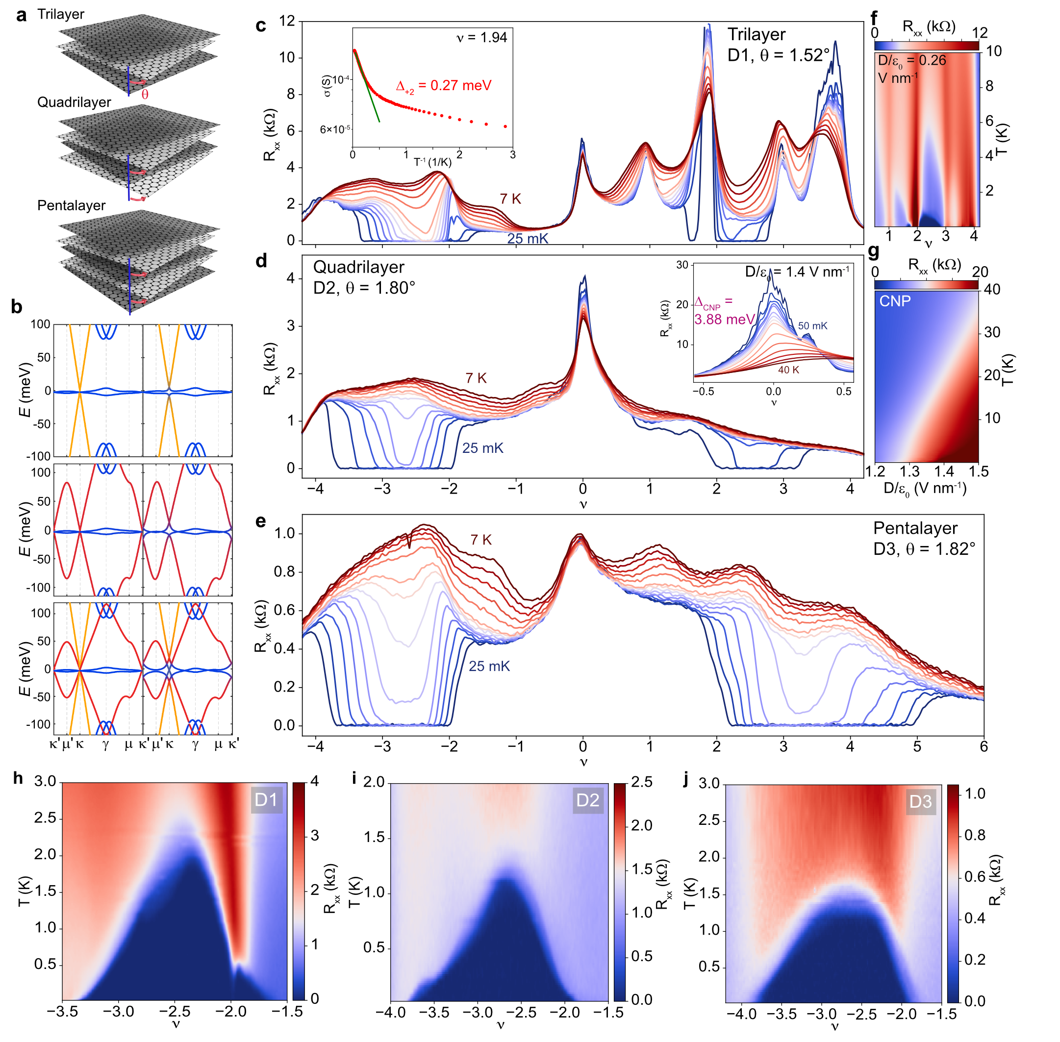
Figure 1: Superconductivity and correlated insulators in alternating twisted graphene multilayers. a, Schematics of the alternating twisted graphene multilayers where each successive layer is twisted by an angle $\pm\theta$ relative to the previous one in an alternating sequence. b, Band structure of twisted trilayer, quadrilayer, and pentalayer graphene (from top to bottom) for angles close to theoretical magic angle at zero $D$ field (left) and $D/\epsilon_{0}\approx 0.4~{}\text{V nm}^{-1}$ (right) for valley K (see SI, section 4). c–e, Line cuts of $R_{xx}$ versus filling factor $\nu$ for a range of temperatures (shown are traces taken first at $25$ mK, then every $0.25$ K from $0.25$ K to $2$ K, followed by every $1$ K from $3$ K to $7$ K), from top to bottom measured at $D/\epsilon_{0}=0.22~{}\text{V nm}^{-1}$ (c), $-0.15~{}\text{V nm}^{-1}$ (d), and $0~{}\text{V nm}^{-1}$ (e), respectively. Activation gap fit of $\nu=+2$ TTG correlated insulator for $D/\epsilon_{0}=0.26~{}\text{V nm}^{-1}$ is shown in inset of c. The inset of d shows insulators in TQG at charge neutrality and larger electric fields. f, $R_{xx}$ versus temperature and $\nu$ for the trilayer focusing around $\nu=+2$ at $D/\epsilon_{0}=0.26~{}\text{V nm}^{-1}$. g, $R_{xx}$ versus temperature and $D$ field for the quadrilayer focusing near charge neutrality. h–j, $R_{xx}$ versus temperature and $\nu$ for hole doping, showing superconducting domes around $\nu=-2$ in the same systems and for the same $D$ fields as in c–e.

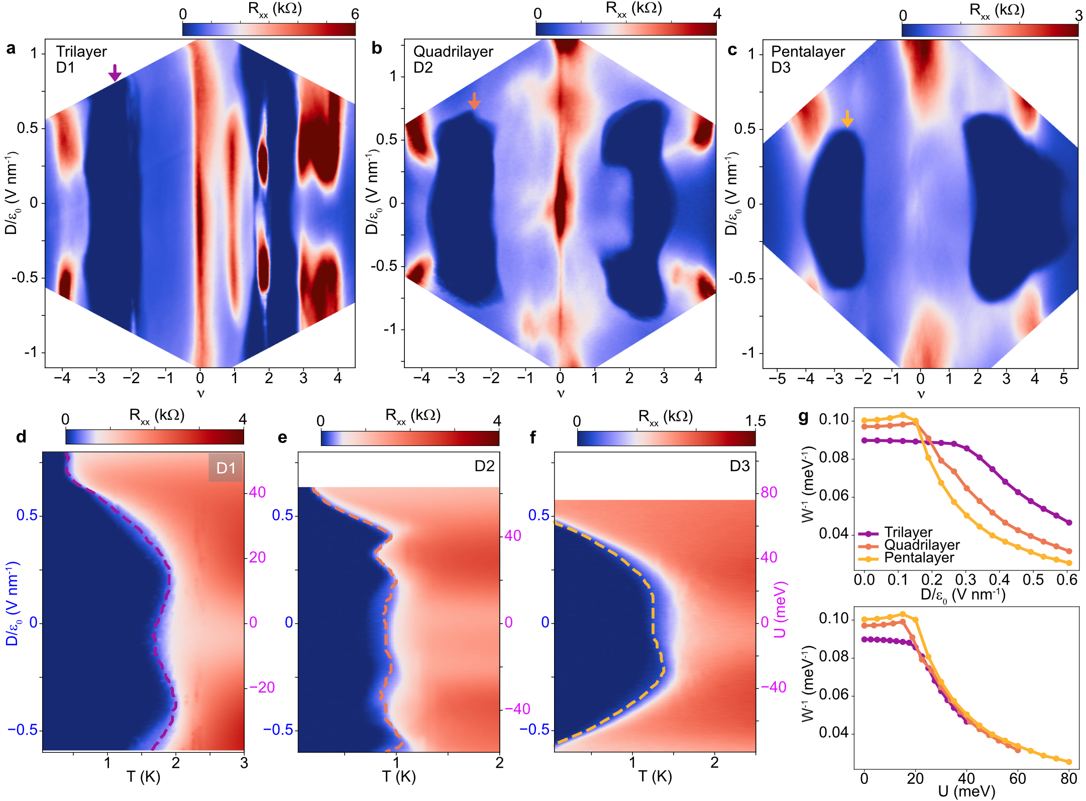
Figure 2: TTG, TQG and TPG phase diagrams and electric field-tunable superconductivity. a–c, $R_{xx}$ versus filling factor $\nu$ and displacement field $D$ for twisted trilayer (a), quadrilayer (b), and pentalayer (c) graphene, respectively. All data are taken at $25$ mK, and the dark blue regions signal superconductivity. For electron-doped TTG and TQG, superconducting regions extend towards $\nu=+1$ at intermediate $D$ field. d–f, $R_{xx}$ versus temperature and $D$ (or equivalent potential difference $U$ between layers, see SI, section 3 for conversion from $D$ to $U$) for the filling factors indicated by arrows in a–c. Critical temperature $T_{c}$ is indicated by a dashed line that delineates $10\%$ of the normal state resistance (see also SI, section 2). $T_{c}$ is maximized at finite $D$ fields. Overall, superconductivity is suppressed more easily with $D$ as the layer number is increased for both hole (d–f) and electron (SI Fig. 5) doping. g, Theoretical calculations of the inverse of the flat-band bandwidth for twisted trilayer, quadrilayer, and pentalayer graphene as a function of $D/\epsilon_{0}$ (top) and potential difference $U$ (bottom). For a fixed $D$, the bandwidth of the flat bands is larger for systems with more layers, but when expressed as a function of $U$, the flat-band broadening follows a similar trend across the different structures. See SI, section 4.1.

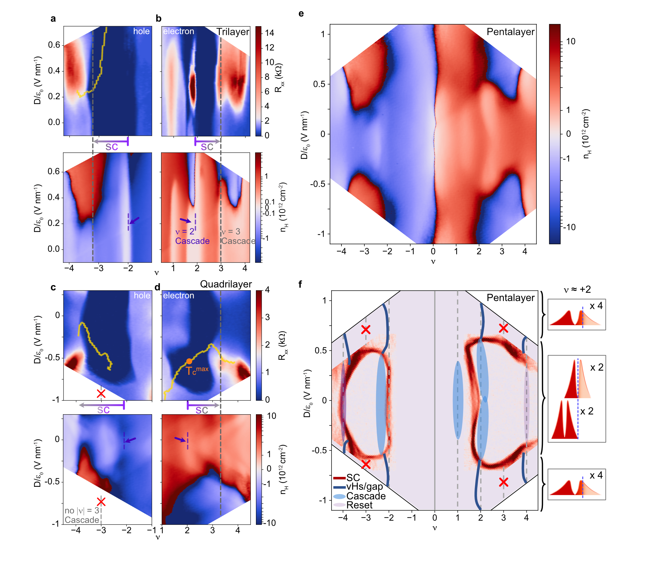
Figure 3: Interplay between superconductivity, flavour symmetry-breaking transitions and van Hove singularities in TTG, TQG and TPG. a,b, $D$ field and $\nu$ dependence of $R_{xx}$ (top) and Hall density (bottom, measured at $B=0.9$ T) for TTG. Purple and grey dashed lines mark the filling factors where flavour symmetry-breaking transitions associated with $|\nu|=2$ and $|\nu|=3$ happen, respectively. The yellow line in a delineates the evolution of the vHs. c,d, $D$ field and $\nu$ dependence of $R_{xx}$ (top) and Hall density (bottom, measured at $B=1.5$ T) for TQG. Superconducting $T_{c}$ reaches its maximum (orange dot in d) exactly at the position of the vHs. When present, flavour symmetry-breaking transitions around $|\nu|\approx 3$ coincide with the termination of superconductivity (a, b, d). By contrast, superconductivity extends much further in the absence of a $|\nu|\approx 3$ reset (c). e, $D$ field and $\nu$ dependence of Hall density for TPG measured at $B=1.5$ T. f, Schematic of Hall density (e) and $R_{xx}$ (Fig. 2c) features for the pentalayer, including the superconducting boundary (red), vHs/‘gap’ (dark blue), cascade (light blue), and $|\nu_{\mathrm{flat}}|=4$ Hall density reset (light purple). Sketches of the DOS around $\nu=+2$ for different $D$ fields are shown on the right. The middle figure illustrates the flavour symmetry polarization observed in regions that support superconductivity. Flavour symmetry is preserved at higher $D$ fields, as shown in the top and bottom images.

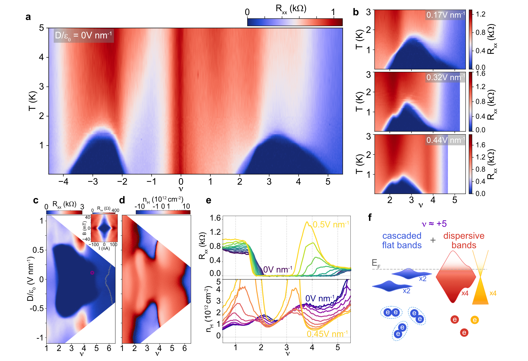
Figure 4: Extended superconducting pockets in TPG. a, $R_{xx}$ versus $\nu$ and temperature at zero $D$ field for twisted pentalayer graphene. b, $R_{xx}$ versus temperature and $\nu$ on the electron side at $D/\epsilon_{0}=0.17$, $0.32$, and $0.44~{}\text{V nm}^{-1}$. The evolution of the superconducting domes and resistance peaks near $\nu=+2$ and $\nu=+4$ with $D$ is shown. c,d, $D$ field and $\nu$ dependence of $R_{xx}$ (c) and Hall density (d, measured at $B=1.5$ T), showing the region around the electron-side superconducting pocket. The grey line in c marks the vHs originating from the dispersive TBG-like bands (see also SI Fig. 10). The inset plots the Fraunhofer-like interference at $\nu=+4.6$, $D/\epsilon_{0}=0.12~{}\text{V nm}^{-1}$ (marked by a red dot in the main panel), confirming the robustness of the superconductivity above $\nu=+4$. e, Line cuts of $R_{xx}$ (top) and Hall density (bottom, measured at $T=1.5$ K, $B=0.5$ T) versus $\nu$ for a range of $D$ fields (traces are shown for every $0.05~{}\text{V nm}^{-1}$ for both $R_{xx}$ and Hall density). Both the presence of Hall density resets around $\nu=+4$ and the development of superconductivity extending from $\nu=+2$ to $+5$ are shown to persist for a wide range of $D$ fields. f, Schematic of scenario $(ii)$ with a Hartree correction for superconductivity at $\nu\approx+5$. The Hartree correction shifts the dispersive TBG- and MLG-like bands down in energy, which causes the flat TBG-like bands to fill more slowly with doping, thus allowing them to host superconductivity at $\nu>+4$.

Supplementary Information:
Ascendance of Superconductivity in Magic-Angle Graphene Multilayers
Yiran Zhang, Robert Polski, Cyprian Lewandowski, Alex Thomson, Yang Peng, Youngjoon Choi, Hyunjin Kim, Kenji Watanabe, Takashi Taniguch, Jason Alicea, Felix von Oppen, Gil Refael, and Stevan Nadj-Perge

1 Device Uniformity and Twist Angle Assignment

Device homogeneity and effect of WSe₂: All devices investigated here show a high degree of twist angle homogeneity as characterized by four-point measurements between different pairs of contacts. SI Fig. 1 shows $R_{xx}$ versus carrier density with fixed top-gate voltage (V${}_{\textsubscript{tg}}$ = 0 V), revealing that almost every pair of contacts shows superconductivity. More importantly, superconducting pockets from different pairs significantly overlap in the filling range, and resistance peaks at $|\nu|=4$ appear at the same density. Moreover, all findings related to the extent of the superconducting phase and the occurrence of the symmetry-breaking transitions in the $\nu$–$D$ phase diagram are highly reproducible. This also includes the observation of a gapped correlated insulator at $\nu=+2$ in TTG, which has not been reported previously. In this context, we note that any significant twist-angle disorder would create conducting percolation pathways that quickly suppress insulating behaviour.

We attribute the low level of disorder to the use of monolayer WSe₂ during device stacking, presumably originating from the increased lateral friction between WSe₂ and graphene (compared to the friction at the hBN-graphene interface). We note that this additional layer does not change the magic-angle condition[14, 6], and the induced spin-orbit interaction (SOI) energy scale is $\sim 1$ meV in twisted bilayers[14]. Therefore, SOI is likely too small to significantly affect the overall band structure and directly impact the cascade physics. Finally, we note that, in general, SOI is expected to manifest differently when the sign of $D$ field is reversed, a feature that has not been observed in the experiment.

Twist angle assignment in multilayers: Twist angles were determined from high $B$ field data and corresponding Landau-fan diagrams in a similar way as in TBG. From the slope of the Landau fan at charge neutrality (which is directly proportional to the gate-sample capacitance) and the voltage difference between charge-neutrality point (CNP) and $|\nu|=4$ filling, the corresponding $|\nu|=4$ electron density is obtained. We used two separate criteria for the assignment of $|\nu|$ = 4. First, at high $D$ fields, resistive features (peaks) emerge (Fig. 2a-c). We interpret these peaks presumably as the opening of the hybridization gaps and corresponding full filling ($|\nu|=4$) of the ‘gapped’ bands. Second, at high $B$ fields, quantum Hall insulating states develop around $|\nu|=4$, which typically cover a broader filling range where Hall conductance is quantized in accordance with the expectations from the dispersive bands (SI Fig. 2, also see discussion below). Electron density of $|\nu|=4$ directly determines the twist angle in the low-angle approximation $\theta^{2}\approx\sqrt{3}a^{2}n_{|\nu|=4}/8$, where $a=0.246$ nm is the graphene lattice constant. We note that signatures of the dispersive bands are also observed in Landau-fan diagrams (SI Fig. 2). For example, emerging Landau levels from the dispersive bands are typically observed through oscillations at low magnetic field. Since at low energies, the dispersive bands (Fig. 1b left) can be effectively treated as decoupled MLG-like bands when considering the Landau level spectrum[35], and the corresponding Hall conductance around $|\nu|=4$ will be quantized in a way that depends on the number of layers (see SI Fig. 2g-m for Hall conductance line cuts).

2 Determining $\mathbf{T_{c}}$ and Hall density

$\mathbf{T_{c}}$ and the coherence length: $T_{c}$ is determined by the following procedures. First, the high temperature $R_{xx}$ data is fitted using a linear function $R(T)=AT+B$. Then, $T_{c}$ is defined by the value where $R_{xx}(T)$ is a certain fraction (typically $10\%$ as in Fig. 2) of $R(T)$. Ginzburg-Landau coherence lengths $\xi_{\mathrm{GL}}$ are obtained from the $B$ dependence of $T_{c}$, by fitting the Ginzburg-Landau relation $T_{c}/T_{c0}=1-(2\pi\xi_{\mathrm{GL}}^{2}/\Phi_{0})B_{\perp}$, where $\Phi_{0}=h/(2e)$ is the superconducting flux quantum and $T_{c0}$ is the critical temperature at zero magnetic field. We get $\xi_{\mathrm{GL}}$ from the $T_{c}$ vs. $B$ linear fit, where the intercept at the $B$ axis is equal to $\Phi_{0}/(2\pi\xi_{\mathrm{GL}}^{2})$. Following Ref. 10, we use $T_{c}$ defined by $40\%$ of the normal state resistance to evaluate the coherence length data in SI Fig. 3e (corresponding error bars are evaluated by using $T_{c}$ defined by $30\%$ and $50\%$ of the normal state resistance). As mentioned in the main text, $\xi_{\mathrm{GL}}$ ($B_{c}$) is much smaller (higher) in the twisted graphene multilayers compared to TBG. One possibility for the reduction of $\xi_{\mathrm{GL}}$ is the relative decrease of the characteristic moiré wavelength (see SI Fig. 3f).

Hall density analysis: Hall density shown in Fig. 3 is obtained by converting the anti-symmetric part of the $R_{xy}$ data, i.e., by subtracting data measured at positive and negative magnetic fields. We used either $|B|=0.9$ T or $1.5$ T in order to fully suppress superconductivity. Previously, it was found that in TTG[10], at high $D$ fields superconductivity is bounded by regions corresponding to vHs, i.e., when Hall density changes sign. We approximately find a similar trend in our TTG and TPG structures, although vHs occasionally intrude superconducting pockets slightly. We note that the exact positions of vHs depend on the precise magnetic field used in the measurements (for example, see SI Fig. 9a and c); however, this effect is relatively small relative to the observed intrusions. More importantly, TQG behaviour is qualitatively different, as we find that positions of vHs and boundaries of superconducting pockets are independent. We also note that resets associated with the flavour polarization do not move in the $B$ fields ($B\approx 1$T) used to extract Hall density evolution. The occasional shift of these resets from integer $\nu$ values, may be attributed to either effects of interactions (i.e. Hartree correction, see section 4.5) or the details of cascade physics[3] at finite temperatures[36, 37].

3 Insulating Behaviour in TTG and TQG

$\mathbf{\nu=+2}$ correlated insulators in TTG: In our TTG device, we observed a previously unidentified $\nu=+2$ correlated insulator state (Fig. 1f and Fig. 1c inset). This state is highly sensitive to $D$ field with maximum activation gap reaching $\Delta_{+2}=0.27$ meV (see SI Fig. 4 for detailed $D$ and $\nu$ dependence). Also, both in-plane and out-of-plane $B$ field suppress the insulating behaviour. These experimental observations are highly indicative of a gap that originates from strong interactions in TTG. Since it is pinned to $\nu=+2$, it likely shares the same underlying origin as the TBG gap found at half filling[1]. We note, however, that formation of the fully gapped states in TTG requires a mechanism that additionally gaps out the MLG-like band, which may explain the presence of the gap only at finite $D$ fields. Moreover, suppression of the gap with magnetic field is at odds with the $C_{2}$ breaking scenario[2, 38] and is more in line with incommensurate Kekulé spiral[39] or intervalley-coherent[40, 41, 16, 15] orders in the flat bands. Finally, we can in part rule out that the gap originates from induced SOI. For example, terms corresponding to Rashba SOI change sign upon $D$-field inversion, yet experimentally we find similar gap values for both positive and negative $D$ fields. However, it is still possible that SOI promotes instabilities that favour the formation for certain $\nu=+2$ insulating states in TTG. Future work will address the nature of this state in more detail.

Charge-neutrality gaps in TQG and conversion between $U$ and $D$: SI Fig. 4f and g shows the charge-neutrality gap of TQG as a function of $D$ field or potential difference $U$ (between the top and the bottom graphene layer). From the continuum model, a gap in TQG is expected when finite $D$ field is applied. However, the details of the gap evolution depend on the precise twist angle. When the twist angle is below the magic-angle value, a charge-neutrality gap opens as soon as a finite $D$ field is applied. On the other hand, when the twist angle is above the magic-angle value, a gap opens only at much higher $D$ fields. The gap opening at $D/\epsilon_{0}\approx 1.1~{}\text{V nm}^{-1}$ in our TQG structure is consistent with the device being slightly above the magic angle. Note that the charge-neutrality gap is a good reference for matching the experimental $D$ field with the potential difference $U$ used in calculations since the interaction-driven Hartree correction vanishes at CNP. For a direct comparison, we enforce a more realistic flat-band bandwidth of $\sim 20$ meV in the continuum model by slightly tuning away from the magic angle, and get a $U$-dependent gap size (SI Fig. 4g). A good match between the experimental and the calculated gap is found when converting $D$ into $U$ with an empirical factor: $U=0.1\times(n-1)\times 0.33~{}{\rm nm}\times eD$, where $e$ is the electron charge and $n-1$ is the number of graphene interfaces. This conversion is used for the other parts of the paper, for example, $T_{c}$ versus $U$ in SI Fig. 5. We note, however, that relative comparison (i.e. scaling) between TTG, TQG, and TPG (in the context of $T_{c}$) does not rely on the precise $D$ to $U$ conversion.

4 Theoretical Calculations

In this section, we describe the non-interacting continuum model for multilayers and how symmetry considerations and various interaction terms affect the band structure of TTG, TQG, and TPG.

4.1 a. Continuum model:

Band structure calculations are performed using a straightforward generalization of the TBG continuum model[42, 43] extended to multilayer graphene systems[8, 44, 45, 46]. As discussed above, we consider graphene multilayer systems with $n_{\mathrm{layer}}=3,4,$ and $5$ layers ($n$ in the main text) in which the graphene sheets are twisted by alternating angles. In particular, we can envision grouping the layers into even and odd sets and then rigidly twisting these two groups by the twist angle $\theta$; equivalently, each layer $\ell=1,\dots,n_{\mathrm{layer}}$ is twisted by an angle $\theta_{\ell}=(-1)^{\ell}\theta/2$. For the moment, we focus on the case where the layers are all AA stack (i.e. stacked directly on top of one another) prior to twisting (see below, section 4.2).

It is appropriate to approximate the dispersion of the underlying graphene monolayers with the two Dirac cones about the valleys at $K$ and $K^{\prime}$. Note that because of the twist, the Dirac cones are located at slightly different momenta depending on whether the layer $\ell$ is even or odd, and we have denoted the Dirac cones’ momenta here as ${\boldsymbol{K}}_{\ell}$ and ${\boldsymbol{K}}_{\ell}^{\prime}$. We thus define the spinors $\psi_{\ell,K^{(\prime)}}$ in terms of the microscopic graphene operators via $f_{\ell}({\boldsymbol{r}})=e^{i{\boldsymbol{K}}_{\ell}\cdot{\boldsymbol{r}}}\psi_{\ell,K}({\boldsymbol{r}})+e^{i{\boldsymbol{K}}_{\ell}^{\prime}\cdot{\boldsymbol{r}}}\psi_{\ell,K^{\prime}}({\boldsymbol{r}})$. Equivalently, in momentum space we can write $\psi_{\ell,K^{(\prime)}}({\boldsymbol{k}})=f_{\ell}({\boldsymbol{k}}+{\boldsymbol{K}}_{\ell}^{(\prime)})$ provided ${\boldsymbol{k}}$ is sufficiently close to ${\boldsymbol{K}}_{\ell}^{(\prime)}$. In our definition of $\psi_{\ell}$ (and $f_{\ell}$) both an A/B sublattice index and a spin index have been suppressed. Importantly, the small twist angle only mediates a very small momentum exchange between the neighbouring layers so that states originating proximate to one valley do not mix with those originating proximate to the other. We thus focus for the moment on valley $K$ and suppress the valley subscript until mentioned otherwise, $\psi_{\ell,K}\to\psi_{\ell}$.

The band structure model can be separated into a sum of two parts: $H_{\mathrm{cont}}=H_{\mathrm{D}}+H_{\mathrm{tun}}$. The first term, $H_{\mathrm{D}}$ is the intralayer Dirac term:

$$H_{\mathrm{D}} =\sum_{\ell=1}^{n_{\mathrm{layer}}}\int d^{2}{\boldsymbol{r}}\,\psi^{\dagger}_{\ell}({\boldsymbol{r}})h_{\mathrm{D},\ell}({\boldsymbol{r}})\psi_{\ell}({\boldsymbol{r}}), h_{\mathrm{D},\ell}({\boldsymbol{r}}) =v_{0}e^{i\theta_{\ell}\sigma^{z}}i\big{(}\partial_{x}\sigma^{x}+\partial_{y}\sigma^{y}\big{)},$$ (1)

Here, $v_{0}\sim 10^{6}\,\text{m/s}$ is the Fermi velocity of the Dirac cones and $\sigma^{x,y,z}$ are Pauli matrices acting on the A/B sublattice indices of the spinors $\psi_{\ell}$. In our simulations, we assume that the Fermi velocity of the graphene monolayers does not differ layer to layer. Note that this assumption, specifically does not take into account effects such as graphene velocity renormalization that can occur in the top layer due to tunnelling between the graphene monolayer and the WSe₂ substrate, as we do not expect these effects to be large enough to have appreciable impact on the resulting band structure.

We assume that tunnelling only occurs between adjacent layers and that it takes the form

$$H_{\mathrm{tun}} =\sum_{\ell=1}^{n_{\mathrm{layer}}-1}\int d^{2}{\boldsymbol{r}}\,\psi^{\dagger}_{\ell}({\boldsymbol{r}})T_{\ell,\ell+1}({\boldsymbol{r}})\psi_{\ell+1}({\boldsymbol{r}})+h.c.$$ (2)

where

$$T_{\ell,\ell+1}({\boldsymbol{r}}) =\sum_{j=1,2,3}e^{-(-1)^{\ell}i{\boldsymbol{q}}_{j}\cdot{\boldsymbol{r}}}t_{j},$$

$${\boldsymbol{q}}_{j} =\frac{4\pi}{3L_{M}}R\left(\frac{2\pi}{3}(j-1)\right)\begin{pmatrix}0\\ -1\end{pmatrix},$$

$$t_{j} =w^{\prime}+w\left(e^{-2\pi(j-1)i/3}\sigma^{+}+e^{-2\pi(j-1)i/3}\sigma^{-}\right).$$ (3)

Here, $R(\phi)=e^{-i\phi\sigma^{y}}$ is a $2\times 2$ rotation matrix acting on vector indices, $L_{M}=a/[2\sin(\theta/2)]$ is the moiré lattice constant, and $\sigma^{\pm}=(\sigma^{x}\pm i\sigma^{y})/2$ act on the sublattice indices. The parameters $w^{\prime}$ and $w$ set the interlayer tunnelling strength; we discuss their values below. It will be convenient to define the dimensionless ratios

$$\eta =\frac{w^{\prime}}{w}\mathbin{\raisebox{2.15277pt}{,}} \alpha =\frac{w}{v_{0}k_{\theta}}\mathbin{\raisebox{2.15277pt}{,}}$$ (4)

where $k_{\theta}=4\pi/(3L_{M})=2\sin(\theta/2)\cdot 4\pi/(3a)$. The total Hamiltonian may be written in matrix form as

$$H_{Tn_{\mathrm{layer}}G} =H_{\mathrm{D}}+H_{\mathrm{tun}}=\sum_{\ell,\ell^{\prime}=1}^{n_{\mathrm{layer}}}\int d^{2}{\boldsymbol{r}}\,\psi^{\dagger}_{\ell}({\boldsymbol{r}})\left[h_{\mathrm{cont}}({\boldsymbol{r}})\right]_{\ell,\ell^{\prime}}\psi_{\ell^{\prime}}({\boldsymbol{r}})$$

$$h_{Tn_{\mathrm{layer}}G}({\boldsymbol{r}}) =\begin{pmatrix}h_{\mathrm{D},1}({\boldsymbol{r}})&T_{1,2}({\boldsymbol{r}})&0&\ldots\\ T^{\dagger}_{1,2}({\boldsymbol{r}})&h_{\mathrm{D},2}({\boldsymbol{r}})&T_{2,3}({\boldsymbol{r}})&\ldots\\ 0&T_{2,3}^{\dagger}({\boldsymbol{r}})&h_{\mathrm{D},3}({\boldsymbol{r}})&\ldots\\ \vdots&\vdots&\vdots&\ddots\end{pmatrix}$$ (5)

As currently written, the diagonal Dirac terms, $h_{\mathrm{D},\ell}({\boldsymbol{r}})$, as well as the off-diagonal tunnelling terms, $T_{\ell,\ell^{\prime}}({\boldsymbol{r}})$, depend only on whether $\ell$ is even or odd. We can thus simplify the above expression by writing the Dirac terms as $h_{\mathrm{D},2\ell-1}({\boldsymbol{r}})=h_{\mathrm{D},1}({\boldsymbol{r}})$, $h_{\mathrm{D},2\ell}({\boldsymbol{r}})=h_{\mathrm{D},2}({\boldsymbol{r}})$ and the tunnelling terms as $T_{2\ell-1,2\ell}({\boldsymbol{r}})=T({\boldsymbol{r}})$, $T_{2\ell,2\ell+1}({\boldsymbol{r}})=T^{\dagger}({\boldsymbol{r}})$.

It has been shown[8] that a block diagonal form exists for Hamiltonians of the form Eq. (4.1). We provide the specific transformations used for three, four, and five layers below.

Twisted bilayer graphene Since the spectrum of the twisted multilayers breaks into independent sets of TBG- and MLG-like bands, we first briefly review the Hamiltonian of TBG. Thus, we start with

$$h_{\alpha,\eta,\theta}({\boldsymbol{r}}) \equiv h_{\mathrm{TBG}}({\boldsymbol{r}})=\begin{pmatrix}h_{\mathrm{D},1}({\boldsymbol{r}})&T({\boldsymbol{r}})\\ T^{\dagger}({\boldsymbol{r}})&h_{\mathrm{D},2}({\boldsymbol{r}})\end{pmatrix}.$$ (6)

Provided that inversion and time reversal symmetries are preserved, the Dirac cones described by $h_{\mathrm{D},\ell}({\boldsymbol{r}})$ at ${\boldsymbol{K}}_{\ell}$ are preserved even when the interlayer tunnelling is added. Nevertheless, this tunnelling term breaks the (effective) continuous translation symmetry of $h_{\mathrm{D},\ell}$. Consequently, the set of conserved momenta are confined to reduced moiré Brillouin zone (BZ). Like the original monolayer graphene BZ, the moiré BZ forms a hexagon with the Dirac cones located at the corners. Here, we define ${\boldsymbol{K}}_{1}={\boldsymbol{\kappa}}$ and ${\boldsymbol{K}}_{2}={\boldsymbol{\kappa}}^{\prime}$ (for the other valley, ${\boldsymbol{K}}_{1}^{\prime}={\boldsymbol{\kappa}}^{\prime}$, ${\boldsymbol{K}}_{2}^{\prime}={\boldsymbol{\kappa}}$).

For small twist angles, the intralayer Dirac terms are nearly identical, $h_{\mathrm{D},\ell}({\boldsymbol{r}})\approx h_{\mathrm{D}}({\boldsymbol{r}})=v_{0}(i\partial_{x}\sigma^{x}+i\partial_{y}\sigma^{y})$—namely, the rotation in Eq. (1) may be neglected to first order. In this case, the spectrum depends solely on the ratios $\eta=w^{\prime}/w$ and $\alpha=w/(\hbar v_{0}k_{\theta})$, where $k_{\theta}=4\pi/(3L_{M})$ is the distance separating $\kappa$ and $\kappa^{\prime}$. Further, as shown in Ref. 43, the spectrum close to Dirac points at $\kappa$ and $\kappa^{\prime}$ can be approximated using a simple perturbative scheme. In particular, in momentum space one finds

$$h_{\mathrm{fl}}({\boldsymbol{k}}+{\boldsymbol{\kappa}}^{(\prime)}) \approx v_{\alpha,\eta}(k_{x}\sigma^{x}+k^{y}\sigma^{y}), v_{\alpha,\eta} =\frac{1-3\alpha^{2}}{1+3\alpha^{2}(1+\eta^{2})}v_{0}.$$ (7)

The magic angle is defined[43] by the condition $v_{\alpha,\eta}=0$, which we see here should occur for $\alpha\approx 1/\sqrt{3}$.

Twisted trilayer graphene

The Hamiltonian for the three layer system is

$$h_{\mathrm{TTG}}({\boldsymbol{r}}) =\begin{pmatrix}h_{\mathrm{D},1}({\boldsymbol{r}})&T({\boldsymbol{r}})&0\\ T^{\dagger}({\boldsymbol{r}})&h_{\mathrm{D},2}({\boldsymbol{r}})&T^{\dagger}({\boldsymbol{r}})\\ 0&T({\boldsymbol{r}})&h_{\mathrm{D},1}({\boldsymbol{r}})\end{pmatrix}.$$ (8)

It maybe be transformed into a block diagonal form as

$$\tilde{h}_{\mathrm{TTG}}({\boldsymbol{r}}) =V_{\mathrm{TTG}}^{\dagger}h_{\mathrm{TTG}}({\boldsymbol{r}})V_{\mathrm{TTG}}=\begin{pmatrix}h_{\sqrt{2}\alpha,\eta,\theta}({\boldsymbol{r}})\\ &h_{\mathrm{D},1}({\boldsymbol{r}})\end{pmatrix},$$

$$V_{\mathrm{TTG}} =\frac{1}{\sqrt{2}}\begin{pmatrix}1&0&1\\ 0&\sqrt{2}&0\\ 1&0&-1\end{pmatrix}.$$ (9)

First, we note that the TTG spectrum separated into independent sets of bands—a TBG-like set described by the two-layer Hamiltonian $h_{\sqrt{2}\alpha,\eta,\theta}$ (an $8\times 8$ object when sublattice and spin are included) and an MLG-like Dirac cone described by $h_{\mathrm{D},1}$. Using the reasoning above, we expect a set of flat TBG-like bands to occur when $\sqrt{2}\alpha=1/\sqrt{3}$. Equivalently, we can assign an effective TBG twist angle describing these bands, $\theta_{\mathrm{TBG}}^{\mathrm{eff}}=\theta/\sqrt{2}$ where $\theta$ is the physical twist angle of the system. If $\theta^{\mathrm{eff}}_{\mathrm{TBG}}$ is expected to yield flat bands in TBG, then we would similarly expect $\sqrt{2}\theta_{\mathrm{TBG}}^{\mathrm{eff}}$ to yield a set of flat bands in TTG.

Twisted quadrilayer graphene For four layers, we start with

$$h_{\mathrm{TQG}}({\boldsymbol{r}}) =\begin{pmatrix}h_{\mathrm{D},1}({\boldsymbol{r}})&T({\boldsymbol{r}})&0&0\\ T^{\dagger}({\boldsymbol{r}})&h_{\mathrm{D},2}({\boldsymbol{r}})&T^{\dagger}({\boldsymbol{r}})&0\\ 0&T({\boldsymbol{r}})&h_{\mathrm{D},1}({\boldsymbol{r}})&T({\boldsymbol{r}})&\\ 0&0&T^{\dagger}({\boldsymbol{r}})&h_{\mathrm{D},2}({\boldsymbol{r}})\end{pmatrix}.$$ (10)

With the appropriate change of basis, we obtain

$$\tilde{h}_{\mathrm{TQG}}({\boldsymbol{r}}) =V_{\mathrm{TQG}}^{\dagger}h_{\mathrm{TQG}}({\boldsymbol{r}})V_{\mathrm{TQG}}=\begin{pmatrix}h_{\varphi\alpha,\eta,\theta}({\boldsymbol{r}})\\ &h_{\varphi^{-1}\alpha,\eta,\theta}({\boldsymbol{r}})\end{pmatrix},$$

$$V_{\mathrm{TQG}} =\frac{1}{\sqrt{1+\varphi^{2}}}\begin{pmatrix}1&0&-\varphi&0\\ 0&\varphi&0&-1\\ \varphi&0&1&0\\ 0&1&0&\varphi\end{pmatrix},$$ (11)

where $\varphi=(1+\sqrt{5})/2$ is the golden ratio. In this case, we therefore expect the TQG spectrum to possess two sets of TBG-like bands characterized by effective TBG twist angles $\theta/\varphi$ and $\theta/\varphi^{-1}$.

Twisted pentalayer graphene The final system considered is the twisted pentalayer graphene. In the original layer basis, the Hamiltonian is

$$h_{\mathrm{TPG}}({\boldsymbol{r}}) =\begin{pmatrix}h_{\mathrm{D},1}({\boldsymbol{r}})&T({\boldsymbol{r}})&0&0&0\\ T^{\dagger}({\boldsymbol{r}})&h_{\mathrm{D},2}({\boldsymbol{r}})&T^{\dagger}({\boldsymbol{r}})&0&0\\ 0&T({\boldsymbol{r}})&h_{\mathrm{D},1}({\boldsymbol{r}})&T({\boldsymbol{r}})&0\\ 0&0&T^{\dagger}({\boldsymbol{r}})&h_{\mathrm{D},2}({\boldsymbol{r}})&T^{\dagger}({\boldsymbol{r}})\\ 0&0&0&T({\boldsymbol{r}})&h_{\mathrm{D},1}({\boldsymbol{r}})\end{pmatrix}.$$ (12)

Once more, independent, co-existing TBG- and MLG-like subsystems are revealed with the appropriate change of basis:

$$\tilde{h}_{\mathrm{TPG}}({\boldsymbol{r}}) =V^{\dagger}_{\mathrm{TPG}}h_{\mathrm{TPG}}({\boldsymbol{r}})V_{\mathrm{TPG}}=\begin{pmatrix}h_{\sqrt{3}\alpha,\eta,\theta}({\boldsymbol{r}})\\ &h_{\mathrm{D},1}({\boldsymbol{r}})\\ &&h_{\alpha,\eta,\theta}({\boldsymbol{r}})\end{pmatrix}$$

$$V_{\mathrm{TPG}} =\frac{1}{\sqrt{6}}\begin{pmatrix}1&0&\sqrt{2}&\sqrt{3}&0\\ 0&\sqrt{3}&0&0&\sqrt{3}\\ 2&0&-\sqrt{2}&0&0\\ 0&\sqrt{3}&0&0&-\sqrt{3}\\ 1&0&\sqrt{2}&-\sqrt{3}&0\end{pmatrix}.$$ (13)

There are now two independent TBG-like bands characterized by effective twist angles $\theta/\sqrt{3}$ and $\theta$ in addition to a MLG-like Dirac cone.

Model Parameters As indicated in Eq. (7), the magic-angle value is essentially determined by the velocity of monolayer graphene $v_{0}$ and the interlayer tunnelling amplitude $w$. We fix $v_{0}$ for all considered configurations. The magnitude of the interlayer tunnelling amplitude is typically estimated to be around $\sim 100$ meV. In case of TQG, a gap is expected to open at charge neutrality when finite $D$ field is applied. However, it onsets for any $|D|>0$ when the physical angle $\theta$ is less than $\varphi\theta_{\mathrm{TBG}}^{\mathrm{magic}}$, where $\theta_{\mathrm{TBG}}^{\mathrm{magic}}$ is the magic angle for TBG (as determined by $v_{0}$ and $w$). When $\theta$ is larger than $\varphi\theta_{\mathrm{TBG}}^{\mathrm{magic}}$, a gap still opens, but only above certain finite $D$ fields. As SI Fig. 4 and SI Fig. 7j show, the latter scenario is observed in the TQG, device D2 (twist angle $1.8\degree$), leading us to select $w=108$ meV near the value used in Ref. 43. In particular, in the left panel of SI Fig. 7j, the $R_{xx}$ is plotted as a function of $D$ field, displaying non-monotonic behaviour—a resistance dip around $D/\epsilon_{0}\sim 0.5$ V nm^-1 followed by a steep increase at higher $D$, signalling the development of an insulating gap. Analogous trends are repeated on the right of SI Fig. 7j, which shows an increase in $\nu=0$ DOS (corresponding to the resistance dip) followed by a decrease to zero DOS.

Similar reasoning can be applied to the TTG and TPG samples, although it is slightly more nebulous since a non-interacting gap is not expected to open in TTG and TPG for any $D$ value at the CNP. Instead, when $\theta>\sqrt{2}\theta_{\mathrm{TBG}}^{\mathrm{magic}}$ for TTG and $\theta>\sqrt{3}\theta_{\mathrm{TBG}}^{\mathrm{magic}}$ for TPG, the system should become metallic with increasing $D$, whereas in the converse situation, the $D$ field should immediately gap out all states except for a dispersive MLG-like Dirac cone. Following this line of reasoning, the results of SI Fig. 7 suggest that the twist angle in TTG is below the magic angle, whereas the one in the TPG sample is above the magic angle. Accordingly, we select $w=110$ meV for TTG and $w=102$ meV for TPG modeling. Notably, the resistance behaviour and theoretical DOS shown in SI Fig. 7k for TPG are very similar to the results in SI Fig. 7j with the primary distinction being that the high-displacement field state does not display the activated transport of an insulator. Similarly, although not obvious from the DOS plot itself, the band structure of TPG at large $D$ is semimetallic (as opposed to insulating).

The value of the interlayer AA hopping $w^{\prime}$ is expected to be less than the interlayer AB hopping, as a result of lattice relaxation (see next section). We chose $w^{\prime}=60$ meV for all three multilayers considered, which is in agreement with the estimates of Ref. 24 and similar to values used previously for TBG/WSe₂ structures[14].

We note that, while consistent with experiment in the fashion outlined about, other factors could be also at play, modifying the behaviour at CNP in ways not captured by our analysis. Ultimately, however, the choices made here are not expected to greatly influence any of the results in this section.

4.2 b. Relative stacking:

An important distinction between TBG and graphene moiré heterostructures containing additional layers is the band structure dependence of the relative layer displacement. Not only must the graphene sheets be stacked with alternating angles, as discussed in the main text and in the previous section, but moreover, the emergence of independent TBG- and Dirac-like bands only occurs when all odd (even) layers are AA stacked, i.e., stacked directly on top of one another. As stated above, we envision grouping the layers into odd and even sets, each stacked rigidly atop one another. The two sets are then twisted relative to one another by the twist angle $\theta$. We have assumed that this stacking was realized in the previous presentation and now argue for the feasibility of this assumption.

In TTG, it has been numerically shown that this situation is energetically preferable: the system naturally relaxes into the odd/even aligned stacking configuration[44]. This result is further experimentally verified in transport[10] and local probe[18] measurements. A simple heuristic supports these results and permits a generalization to additional layers. Starting from a bilayer system, the moiré superlattice is manifest on the microscopic lattice scale as the periodic variation of the relative interlayer stacking: one has AA regions at the moiré hexagon centres, while AB and BA stacking regions represent the moiré hexagon vertices. The AA regions have a relatively high energy compared to the Bernal-like region and the lattice accordingly responds by relaxing to minimize their area. We now consider adding a third layer with the same relative twist angle as the first layer, but for the moment arbitrarily displaced from that layer. A moiré superlattice is of course also generated between the new layer and the second layer, and the system once again seeks to minimize (maximize) the area of the AA (AB/BA) regions. Crucially, if the first and third layers are misaligned, the AA regions between the first and second layers are misaligned from the AA regions between the second and third layers, frustrating the ability of the lattice to relax. Only when the first and third layers are aligned will the AA region occur at the same locations and only then can the system optimize its energy through relaxation. These arguments clearly generalize to quadrilayer and pentalayer systems—we need only consider the moiré pattern generated by each adjacent pair of graphene sheets to conclude that relaxation is optimized by an odd/even aligned configuration. (A complementary explanation is that TTG is necessarily an intermediate step in the construction of the TQG and TPG devices, and thus the odd alignment is already baked into a subset of the layers.)

4.3 c. Mirror symmetry:

In the systems with an odd number of layers, an onsite mirror symmetry is present, which acts as

$$\psi({\boldsymbol{r}}) \to U_{\mathrm{mirror}}^{(n_{\mathrm{layer}})}\psi({\boldsymbol{r}}), n_{\mathrm{layer}}\text{ odd},$$ (14)

where

$$\left[U_{\mathrm{mirror}}^{(n_{\mathrm{layer}})}\right]_{\ell,\ell^{\prime}} =\delta_{\ell,n_{\mathrm{layer}}-\ell^{\prime}+1}.$$ (15)

Here, $\ell$, $\ell^{\prime}$ label the system’s layers. Effectively, this operator simply flips the layers around, for instance, interchanging layers 1 and 3 in TTG, while keeping the middle layer fixed. In terms of the matrices, this invariance manifests simply as the relation $[h_{\mathrm{TTG}}({\boldsymbol{r}}),U_{\mathrm{mirror}}^{(3)}]=0$ and $[h_{\mathrm{TPG}}({\boldsymbol{r}}),U_{\mathrm{mirror}}^{(5)}]=0$. As we see below, the preservation of this symmetry is inextricably tied to the block diagonal form of the TTG continuum model presented in Eq. (4.1). In particular, rotating $U_{\mathrm{mirror}}^{(3)}$ to the subsystem basis defined by $V_{\mathrm{TTG}}$ returns $\tilde{U}_{\mathrm{mirror}}^{(3)}=V_{\mathrm{TTG}}^{T}U_{\mathrm{mirror}}^{(3)}V_{\mathrm{TTG}}=\mathrm{diag}(1,1,-1)$. The TBG-like subsystem corresponds precisely to the even parity sector (i.e., has eigenvalue $+1$ under the action the mirror symmetry) whereas the dispersive MLG-like subsystem belongs to the odd parity sector (i.e., has eigenvalue $-1$ under the action the mirror symmetry). The TBG- and MLG-like bands thus cannot hybridize without breaking this symmetry.

We can similarly rotate the TPG operator, $U^{(5)}_{\mathrm{mirror}}$ to the subsystem basis $\tilde{U}_{\mathrm{mirror}}^{(5)}=V_{\mathrm{TPG}}^{T}U_{\mathrm{mirror}}^{(5)}V_{\mathrm{TPG}}$, yielding $\tilde{U}_{\mathrm{mirror}}^{(5)}=\mathrm{diag}(1,1,1,-1,-1)$. Comparing against Eq. (4.1), we observe that both the TBG-like subsystem with effective twist angle $\theta/\sqrt{3}$ and the MLG-like subsystem belong to the even parity sector, whereas the subsystem with effective twist angle $\theta$ belongs to the odd parity sector. The mirror symmetry therefore only protects the latter subsystem—which is notably not at the magic angle in the experiment. In other words, in TPG with mirror symmetry, flat TBG-like band and MLG-like band can hybridize (while the dispersive TBG-like band is protected).

A mirror-like symmetry also exists for even-layered systems like TBG and TQG, but it does not act in an onsite fashion and is therefore not useful for the analysis that follows. For TQG, hybridization between subsystems is therefore not prohibited by symmetry.

4.4 d. Band mixing:

In obtaining the independent TBG- and MLG-like bands (subsystems) listed above, a number of assumptions were made and one may be concerned about the relative robustness of these results. For TTG, at least, this question may be dismissed so long as mirror symmetry is present; above, we showed that this mirror symmetry protects the block diagonal subsystem form obtained for TTG. Similarly, mirror symmetry disallows mixing in TPG between certain (but not all) subsystems. However, the mirror symmetry is explicitly broken by the application of a displacement field as well as by the WSe₂ substrate used in the experiment. Below, we show that these modifications induce mixing between all subsystems. We additionally consider other mirror-preserving effects that may result in subsystem mixing in TQG and TPG.

Besides the displacement field, we find that the subsystem-mixing energy scales discussed below are relatively small compared to the input parameters of the continuum model, i.e., compared to an interlayer tunnelling of $w$ and $w^{\prime}$. More importantly, they are also smaller than the observed bandwidth of TBG, which spectroscopic measurements indicate is $\sim 40$ meV for samples close to the magic angle[47, 4, 48, 49]. The subleading magnitude of the effects we explore below thus bolsters our use of the alternating-angle continuum model, at least as a starting point. We note that the relatively small subsystem hybridization discussed here could be significantly magnified by interactions.

Effect of displacement field In the main text, we allude to the fact that a finite displacement field mixes the TBG- and MLG-like subsystems obtained in the previous sections. This effect is included in the Hamiltonian through the addition of

$$H_{\mathrm{disp}} =\sum_{\ell,\ell^{\prime}=1}^{n_{\mathrm{layer}}}\int d^{2}{\boldsymbol{r}}\,\psi^{\dagger}_{\ell}({\boldsymbol{r}})\left[h^{(n_{\mathrm{layer}})}_{\mathrm{disp}}\right]_{\ell,\ell^{\prime}}\psi_{\ell^{\prime}}^{\dagger}({\boldsymbol{r}}), \left[h^{(n_{\mathrm{layer}})}_{\mathrm{disp}}\right]_{\ell,\ell^{\prime}} =U\delta_{\ell,\ell^{\prime}}\left(\frac{1}{2}-\frac{\ell-1}{n_{\mathrm{layer}}-1}\right).$$ (16)

Specifically, we have $h^{(3)}_{\mathrm{disp}}=(U/2)\mathrm{diag}(1,0,-1)$, $h_{\mathrm{disp}}^{(4)}=U\mathrm{diag}(1/2,1/6,-1/6,-1/2)$, and $h^{(5)}_{\mathrm{disp}}=U\mathrm{diag}(1/2,1/4,0,-1/4,-1/2)$. Here, the scale $U$ is defined as outlined in section 3.

Focusing first on the odd-layered systems, TTG and TPG, we observe that this perturbation explicitly breaks the mirror symmetry introduced in the previous section. In particular, $h^{(3)}_{\mathrm{disp}}$ and $h^{(5)}_{\mathrm{disp}}$ anticommute with $U^{(3)}_{\mathrm{mirror}}$ and $U^{(5)}_{\mathrm{mirror}}$ respectively: $\{h_{\mathrm{disp}}^{(3)},U_{\mathrm{mirror}}^{(3)}\}=0$ and $\{h_{\mathrm{disp}}^{(5)},U_{\mathrm{mirror}}^{(5)}\}=0$. The displacement field therefore allows subsystems within different parity sectors to hybridize. The effect of this addition is apparent when $h_{\mathrm{disp}}^{(n_{\mathrm{layer}})}$ is tranformed to the subsystem basis of Eqs. (4.1) and (4.1):

$$\tilde{h}_{\mathrm{disp}}^{(3)} =V_{\mathrm{TTG}}^{\dagger}h_{\mathrm{disp}}^{(3)}V_{\mathrm{TTG}}=\frac{U}{2}\begin{pmatrix}0&0&1\\ 0&0&0\\ 1&0&0\end{pmatrix}\begin{matrix}\left.\begin{matrix}\phantom{\!}\\ \phantom{\!}\end{matrix}\right\}&\!\!\text{Parity-even sector}\\ \left.\phantom{\!}\right\}&\!\!\text{Parity-odd sector}\end{matrix}$$

$$\tilde{h}_{\mathrm{disp}}^{(5)} =V_{\mathrm{TPG}}^{\dagger}h_{\mathrm{disp}}^{(5)}V_{\mathrm{TPG}}=\frac{U}{4\sqrt{3}}\begin{pmatrix}0&0&0&2&0\\ 0&0&0&0&\sqrt{3}\\ 0&0&0&2\sqrt{2}&0\\ 2&0&2\sqrt{2}&0&0\\ 0&\sqrt{3}&0&0&0\end{pmatrix}\begin{matrix}\left.\begin{matrix}\phantom{\!}\\ \phantom{\!}\\ \phantom{\!}\end{matrix}\right\}&\!\!\text{Parity-even sector}\\ \left.\begin{matrix}\phantom{\!}\\ \phantom{\!}\end{matrix}\right\}&\!\!\text{Parity-odd sector}\end{matrix}$$ (17)

We thus explicitly see the way in which the displacement field induces mixing between subsystems.

Subsystem mixing is also a natural consequence of the displacement field in TQG. The Hamiltonian in Eq. (16) takes the form $h_{\mathrm{disp}}^{(4)}=U\mathrm{diag}(1/4,1/6,-1/6,1/4)$, which becomes

$$\tilde{h}_{\mathrm{disp}}^{(4)} =\frac{U}{30\varphi}(1+\varphi^{2})\begin{pmatrix}\varphi^{-3}&0&-4&0\\ 0&-\varphi^{-3}&0&-4\\ -4&0&\varphi^{3}&0\\ 0&-4&0&-\varphi^{3}\end{pmatrix}\begin{matrix}[l]\left.\ \begin{matrix}\phantom{\!}\\ \phantom{\!}\end{matrix}\right\}&\!\!\text{Subsystem with $\theta^{\mathrm{eff}}_{\mathrm{TBG}}=\varphi\theta$}\\ \left.\ \begin{matrix}\phantom{\!}\\ \phantom{\!}\end{matrix}\right\}&\!\!\text{Subsystem with $\theta^{\mathrm{eff}}_{\mathrm{TBG}}=\varphi^{-1}\theta$}\end{matrix}$$ (18)

in the subsystem basis.

Proximity-induced spin-orbit coupling One of the exterior layers of the samples considered here is placed adjacent to WSe₂. This type of construction was first shown to induce spin-orbit coupling in twisted bilayer graphene in Ref. 14. The presence of WSe₂ breaks not only the spin symmetry, but also the mirror symmetry in systems considered here and possibly induces subsystem mixing. The magnitude of the induced spin-orbit scale has been measured to be approximately $1-5$ meV in TBG, smaller than the other scales of the theory (e.g., the band width). In effect, in rotating to the subsystem basis, the spin-orbit terms are “spread” across an increasing number of layers by the unitary transformations $V_{\mathrm{TTG}}$, $V_{\mathrm{TQG}}$, $V_{\mathrm{TPG}}$.

Mirror-symmetric, nonuniform charge distribution: The chemical potentials of the different layers may also differ in a way that is symmetric under onsite mirror actions $U_{\mathrm{mirror}}^{(4/5)}$ of Eq. (15). In particular, we may have $h_{\mu\text{-}\mathrm{var}}^{(4)}=\mathrm{diag}(\delta\mu_{1},\delta\mu_{2},\delta\mu_{2},\delta\mu_{1})$, which takes the subsystem-basis form

$$\tilde{h}_{\mu\text{-}\mathrm{var}}^{(4)} =\frac{\delta\mu}{\sqrt{5}}\begin{pmatrix}-1&0&-2&0\\ 0&-1&0&2\\ -2&0&1&0\\ 0&2&0&1\end{pmatrix},$$ (19)

where $\delta\mu=\delta\mu_{1}=-\delta\mu_{2}$. Similarly, for TPG, a term like $h_{\mathrm{\mu\text{-}\mathrm{var}}}^{(5)}=\mathrm{diag}(\delta\mu_{1},\delta\mu_{2},\delta\mu_{3},\delta\mu_{2},\delta\mu_{1})$ also preserves the mirror operator $U_{\mathrm{mirror}}^{(5)}$ but can be shown to induce inter-subsystem mixing within the even parity sector. As we demonstrate in section 4.5, such a term is naturally generated by the Coulomb interaction. We specify to TPG in that section, but the reasoning is analogous for TQG (and for TTG, although this term will not induce mixing between sectors because of the mirror symmetry).

Although generically present, the Coulomb interaction-generated terms of this form are relatively small compared to the other terms present. The calculations presented below estimate that values of $|\delta\mu_{\ell}|<5-10$ meV for TPG are generated as one dopes away from charge neutrality. We expect the results for TQG to follow the same trend.

Next-nearest layer tunnelling Our Hamiltonian so far only includes tunnelling between neighbouring layers. Generically, however, hopping between next-nearest neighbouring layers occurs as well. For TQG, we could therefore consider hopping between layers 1 (2) and 4 (3):

$$h_{\mathrm{nnl}}^{(4)} =\begin{pmatrix}0&0&T_{\mathrm{nnl}}&0\\ 0&0&0&T_{\mathrm{nnl}}\\ T^{\dagger}_{\mathrm{nnl}}&0&0&0\\ 0&T^{\dagger}_{\mathrm{nnl}}&0&0\end{pmatrix}.$$ (20)

Assuming for simplicity that $T_{\mathrm{nnl.}}=T^{\dagger}_{\mathrm{nnl}}$, in the subsystem basis, this term takes the form

$$\tilde{h}_{\mathrm{nnl}}^{(4)} =\frac{1}{\sqrt{5}}\begin{pmatrix}2T_{\mathrm{nnl}}&0&-T_{\mathrm{nnl}}&0\\ 0&2T_{\mathrm{nnl}}&0&T_{\mathrm{nnl}}\\ -T_{\mathrm{nnl}}&0&-2T_{\mathrm{nnl}}&\\ 0&T_{\mathrm{nnl}}&0&-2T_{\mathrm{nnl}}\end{pmatrix}.$$ (21)

Note that because we assume next-nearest layers are stacked AA relative to one another, to first order, no spatial dependence is expected in $T_{\mathrm{nnl}}$. The subsystems are similarly mixid with the five-layer analogue $h^{(5)}_{\mathrm{nnl}}$. Reference 44 computed the values of $T_{\mathrm{nnl}}$ expected in TTG (where it will not induce subsystem mixing) and found that a typical scale $|T_{\mathrm{nnl},ij}|\sim 5-10$ meV, which translates to $|T_{\mathrm{nnl},ij}|/\sqrt{5}\sim 3-5$ meV ($i$ and $j$ are sublattice indices).

Lattice relaxation As mentioned in section 4.2, the moiré lattice relaxes in order to minimize AA regions and maximize AB/BA regions. As mentioned, this relaxation effect ultimately depresses the value of $w^{\prime}$ (interlayer AA tunnelling) relative to $w$ (interlayer AB/BA tunnelling) as a result of out-of-plane corrugation. For interior layers, which neighbour more than a single sheet, the effects of relaxation are naturally stronger than for exterior layers. Consequently, the value of $\eta=w^{\prime}/w$ appropriate for tunnelling to and from interior layers is reduced. Our assumption below Eq. (4.1) that $T_{\ell,\ell+1}({\boldsymbol{r}})$ depended only on whether $\ell$ was even or odd is no longer valid. Unsurprisingly, this effect once again mixes the subsystems in TQG and TPG. Reference 24 estimated the magnitude of this effect and determined that it should be in the range $5-10$ meV for the twist angles considered here.

4.5 e. The role of interactions in TPG:

The presence of flat-band subsystem in the low-energy theory of the multilayer graphene structures necessitates the consideration of interaction-driven band structure corrections. In the following, we focus specifically on the case of TPG as its phase diagram demonstrates the strongest deviation from the minimal paradigm that a multilayer structure maybe thought of as a TBG-like Hamiltonian with spectating additional bands. Rather, as we argue, the dispersive TBG- and MLG-like subsystems play a crucial role in extending the filling range of the superconducting pocket in accordance with scenario ($ii$) and ($iii$). Here, we consider three types of interaction corrections: (a) an in-plane Hartree correction; (b) a two-parameter effective model mimicking generic Hartree-Fock modifications of band structure; (c) an out-of-plane Hartree correction allowing for inhomogeneous charge distribution between the layers. We demonstrate that these effects generically lead to two consequences for the electronic spectrum: promoting charge redistribution to the non-flat bands and also leading to possible symmetry breaking between the non-flat and flat bands.

Hartree correction We begin with an in-plane Hartree effect. As demonstrated experimentally in previous work on TBG[29] and TTG[18], filling-dependent interaction effects, specifically Hartree and Fock corrections, drastically alter the electronic dispersion. Here we incorporate only a Hartree mechanism[25, 26, 27, 28] in the analysis, arguing that its key effect, a relative shift of flat bands up in energy with respect to the non-flat bands, is the simplest mechanism through which the size of the superconducting pocket in TPG is extended. We then supplement this discussion with a phenomenological Hartree-Fock-like theory. Before proceeding, we stress that the main purpose of the analysis in this section is to demonstrate that scenario ($i$) wherein flat bands are filled only to $\nu_{\mathrm{flat}}\approx+3$ at $\nu\approx+5$ is highly unlikely, thus highlighting the non-trivial role played by the dispersive TBG- and MLG-like bands.

The foundations of the Hartree calculation in TPG described below are identical to the analysis in Refs. 29 and 18. We reproduce them here for the convenience of the reader. We introduce the Coulomb interaction into the system through

$$H_{C} =\frac{1}{2}\int d^{2}{\boldsymbol{r}}\,d^{2}{\boldsymbol{r}}^{\prime}\,\delta\rho({\boldsymbol{r}})V({\boldsymbol{r}}-{\boldsymbol{r}}^{\prime})\delta\rho({\boldsymbol{r}}^{\prime}).$$ (22)

In section 4.1, we introduced creation and annihilation operators, $\psi^{\dagger}({\boldsymbol{r}})$ and $\psi({\boldsymbol{r}})$, that correspond to the non-interacting eigenstates given by the Hamiltonian of Eq. (4.1). Here and in what follows, we suppress the layer, valley, sublattice and spin subscripts. In Eq. (22), $V({\boldsymbol{r}})=e^{2}/(\epsilon|{\boldsymbol{r}}|)$ is the Coulomb potential and $\delta\rho({\boldsymbol{r}})=\psi^{\dagger}({\boldsymbol{r}})\psi({\boldsymbol{r}})-\rho_{\mathrm{CN}}({\boldsymbol{r}})$, where $\rho_{\mathrm{CN}}({\boldsymbol{r}})=\langle\psi^{\dagger}({\boldsymbol{r}})\psi({\boldsymbol{r}})\rangle_{\mathrm{CN}}$ is the expectation value of the density at the charge-neutrality point. The use of $\delta\rho({\boldsymbol{r}})$ instead of $\rho({\boldsymbol{r}})$ in the interaction is motivated by the expectation that the input parameters of the model $H_{\mathrm{T}n_{\mathrm{layer}}G}=H_{\mathrm{cont}}$ already include the effect of interactions at the charge-neutrality point. The dielectric constant $\epsilon$ in the definition of $V({\boldsymbol{r}})$ is used as a fitting parameter; see discussion below for details.

We study the effect of the interacting continuum model of magic-angle TPG through a self-consistent Hartree mean-field calculation. Instead of solving the many-body problem, we obtain the quadratic Hamiltonian that best approximates the full model when only the symmetric contributions of $H_{C}$ are included, i.e., the Fock term is neglected. Thus instead of $H_{\mathrm{cont}}+H_{C}$, we study the Hamiltonian

$$H_{\mathrm{MF}}^{(\nu)} =H_{\mathrm{cont}}+H^{(\nu)}_{\mathrm{H}}-\frac{1}{2}\langle H_{\mathrm{H}}^{(\nu)}\rangle_{\nu},$$ (23)

where $H_{\mathrm{H}}^{(\nu)}$ is the Hartree term at filling $\nu$,

$$H_{\mathrm{H}}^{(\nu)} =\int_{{\boldsymbol{k}},{\boldsymbol{k}}^{\prime},{\boldsymbol{q}}}V({\boldsymbol{q}})\langle\psi^{\dagger}({\boldsymbol{k}}^{\prime}+{\boldsymbol{q}})\psi({\boldsymbol{k}}^{\prime})\rangle_{\nu}\psi^{\dagger}({\boldsymbol{k}})\psi({\boldsymbol{k}}-{\boldsymbol{q}}),$$ (24)

and the last term in Eq. (23) simply ensures there is no double counting when one calculates the total energy. In the above equation, $V({\boldsymbol{q}})=2\pi e^{2}/(\epsilon|{\boldsymbol{q}}|)$ is the Fourier transform of the Coulomb interaction $V({\boldsymbol{r}})$ in Eq. (22), and the expectation value $\langle\hat{\mathcal{O}}\rangle_{\nu}=\langle\hat{\mathcal{O}}\rangle_{\mathrm{occ}}-\langle\hat{\mathcal{O}}\rangle_{\mathrm{CN}}$ only includes states that are filled up to $\nu$ relative to charge neutrality, as defined by diagonalizing the Hamiltonian $H_{\mathrm{MF}}^{(\nu)}$.

Typically, for a “jellium”-like model, the expectation value in Eq. (24) vanishes save for ${\boldsymbol{q}}=0$, which is subsequently cancelled by the background charge—allowing one to set $V({\boldsymbol{q}}=0)=0$ and completely ignore the Hartree interaction. However, because the moiré pattern breaks continuous translation symmetry, momentum is only conserved modulo a reciprocal lattice vector. We therefore obtain

$$H_{\mathrm{H}}^{(\nu)} =\sum_{{\boldsymbol{G}}}^{\prime}V({\boldsymbol{G}})\int_{{\boldsymbol{k}}^{\prime}}\langle\psi^{\dagger}({\boldsymbol{k}}^{\prime}+{\boldsymbol{G}})\psi({\boldsymbol{k}}^{\prime})\rangle_{\nu}\int_{{\boldsymbol{k}}}\psi^{\dagger}({\boldsymbol{k}})\psi({\boldsymbol{k}}-{\boldsymbol{G}}),$$ (25)

where the prime above the summation over the moiré reciprocal lattice vectors indicates that ${\boldsymbol{G}}=0$ is excluded. The self-consistent procedure begins by assuming some initial value of $H_{\mathrm{H}}^{(\nu)}$ and diagonalizing the corresponding mean-field Hamiltonian $H_{\mathrm{MF}}^{(\nu)}$ to obtain the Bloch wavefunctions and energy eigenvalues. These quantities are then used to re-compute the expectation values that define $H_{\mathrm{H}}^{(\nu)}$ and thus $H_{\mathrm{MF}}^{(\nu)}$ subject to the cascade treatment described above. This process is repeated until one obtains the quadratic Hamiltonian $H_{\mathrm{MF}}^{(\nu)}$ that yields the correlation functions $\langle\cdot\rangle_{\nu}$ used in its definition.

Due to the accumulation of electronic density at the $AA$ sites of the stacking sequence, the Hartree potential is dominated by the first ‘star’ of moiré reciprocal lattice vectors[25, 50], which in our conventions corresponds to ${\boldsymbol{G}}_{n}=R\big{(}2\pi(n-1)/6\big{)}\frac{4\pi}{\sqrt{3}L_{M}}(1,0)^{T}$ for $n=1,\dots,6$, with $R(\phi)$ a rotation matrix. The restriction to the ${\boldsymbol{G}}_{n}$’s paired with the $2\pi/6$ rotation symmetry of the continuum model greatly simplifies the calculation of the Hartree term. Notably, $V({\boldsymbol{G}})\int_{{\boldsymbol{k}}^{\prime}}\langle\psi^{\dagger}({\boldsymbol{k}}^{\prime}+{\boldsymbol{G}})\psi({\boldsymbol{k}}^{\prime})\rangle_{\nu}$ must be the same for all ${\boldsymbol{G}}_{n}$, and, instead of Eq. (25), we use

$$H_{\mathrm{H}}^{(\nu)} =V_{\mathrm{H}}^{(\nu)}\sum_{n=1}^{6}\int_{\boldsymbol{k}}\psi^{\dagger}({\boldsymbol{k}})\psi({\boldsymbol{k}}-{\boldsymbol{G}}_{n}), V_{\mathrm{H}}^{(\nu)} =\frac{1}{6}\sum_{n=1}^{6}V({\boldsymbol{G}}_{n})\int_{{\boldsymbol{k}}^{\prime}}\langle\psi^{\dagger}({\boldsymbol{k}}^{\prime}+{\boldsymbol{G}})\psi({\boldsymbol{k}}^{\prime})\rangle_{\nu}\,.$$ (26)

The self-consistent procedure in this case is identical to that described in the previous paragraph, but due to the reduced number of reciprocal lattice vectors that are included in the summation, the calculation is computationally easier. Convergence is typically reached within $\sim 6$ iterations.

We now proceed to discuss the precise effect of the Hartree correction. Since the Hartree correction couples bare graphene states at momenta ${\boldsymbol{k}}$ and ${\boldsymbol{k}}+{\boldsymbol{G}}$, its effect is most pronounced for subsystems of the Hamiltonian whose eigenstates require multiple bare graphene states originating from multiple moiré BZs, e.g. ${\boldsymbol{k}}+{\boldsymbol{G}}$ states with ${\boldsymbol{G}}$ extending beyond the second BZ. As such, Hartree affects the flat-band subsystem most severely since its eigenstates deviate the most from the bare graphene states, while the MLG-like subsystem is affected the least. As a result, this correction gives rise to an energy offset that shifts the flat bands upwards in energy with respect to the rest of the energy spectrum (technically the dispersive TBG-like subsystem is also shifted slightly with respect to the MLG-like subsystem). This effect has been seen both theoretically and experimentally in TTG[30, 18]. Thus we expect it to be present in TPG, as is confirmed through our simulations; see SI Fig. 11a,b. Physically, this effect arises simply because the charge distribution from the non-flat subsystems is more homogeneous in the unit cell and, therefore, it contributes less to the potential of Eq. (24).

We now discuss what happens when one starts from charge neutrality and electron dopes the system. Due to the shift of the flat band upwards in energy relative to the non-flat bands, more charge can enter the non-flat bands upon doping (increasing $\nu$) than a naïve non-interacting model predicts. As a result, the filling range of the flat TBG-like band superconducting pocket may be extended since the filling of the flat bands $\nu_{\mathrm{flat}}$ can continue to lie in the range amenable to superconductivity, whilst the total filling $\nu$ increases by adding charge to the non-flat bands. This is the central idea behind the scenarios ($i$) and ($ii$) discussed in section 5.

In the simulations for flat-band filling $\nu_{\mathrm{flat}}>+2$, we consider two ways to fill the otherwise 4-fold degenerate bands: an uncascaded model where all 4-fold degenerate bands are filled equally, and a simple cascade model where two of the flat-band flavours (say spin $\uparrow$ for $K$, $K^{\prime}$) are shifted down in energy such that the highest energy of the shifted bands falls on the Dirac point of the unshifted flat bands, c.f. SI Fig. 11c. In the absence of Hartree-induced band inversion (as in fact we will consider in the following section), the shifted bands ($\uparrow$ bands) are fully filled at $\nu_{\mathrm{flat}}=+2$ and the unshifted bands ($\downarrow$) and the dispersive bands contain the remaining $\nu-2$ charge. With the Hartree-induced gamma point inversion, the two sets of the flat bands (shifted - $\uparrow$, unshifted - $\downarrow$) become partially filled near $\nu_{\mathrm{flat}}=+2$. The shifted ($\uparrow$) band is mostly filled and the unshifted ($\downarrow$) is mostly empty. This simple approach qualitatively reproduces the effect of a cascade at $|\nu_{\mathrm{flat}}|\approx 2$ under the assumption that the specific nature of the cascade state (i.e. spin or valley polarized) is irrelevant for the consideration of the total filling. We caution, however, that a cascade transition is an effect originating from an interplay between Hartree and Fock corrections (see Ref. 29 for further discussion), and that Fock corrections, which we neglected so far, can give rise to many effects.

The most crucial ones, including bandwidth broadening [50, 51, 52, 53] and gap opening in the flat-band subsystem[4, 54, 51, 40, 15, 41, 16, 55], may actually affect the charge distribution across the different subsystems. These effects are neglected in the current analysis—an approximation we will justify in the following section.

The cascade, as shown in SI Fig. 11g, allows charge to enter the unfilled flat bands more easily compared to the uncascaded ground state. This behaviour is expected since a cascade minimizes the contribution of the Hartree term by redistributing charge away from parts of the flat bands which overlap more strongly with the Hartree potential—in particular, for the parameters considered here and within the relevant range of filling factors, the cascade is the ground state solution. Note, however, that while including only the Hartree correction is sufficient to initiate cascade, Fock must be included in order for it to persist over the experimentally observed range (see Ref. 29 for further discussion on the interplay of Hartree and Fock corrections and the onset of cascade).

To quantitatively estimate the fillings of the different subsystems, it is necessary to parametrize the strength of the Coulomb interaction, e.g., the dielectric constant $\epsilon$ that enters into Eq. (24). Although, in principle, the dielectric constant is fixed primarily by the substrate and any interaction corrections can be accounted for via a self-consistent treatment, in practice[25, 50, 52, 29], it can be treated as a fitting parameter. If a bare value of the interaction is used, then the resulting interaction corrections are too large and lead to unobserved predictions[29, 18]. We use the cascade near $\nu_{\mathrm{flat}}\approx+2$ to constrain $\epsilon$. We identify $\nu_{\mathrm{flat}}=+2$ with the experimental onset of the cascade transition, which occurs near $\nu\approx+2.15$; see Fig. 4e. By choosing $\epsilon$ so that $\nu_{\mathrm{flat}}$ reaches $+2$ at the same point the total filling $\nu$ reaches $+2.15$ (see SI Fig. 11e), we find $\epsilon\approx 11.15$. We emphasize that although this is an approximate fitting relying on the particular model of a cascade, the Hartree-induced flat-band energy shift is a robust and important effect (SI Fig. 11f). Using the value of $\epsilon\approx 11.15$, we find that at $\nu\approx+5$, the flat bands are filled to approximate $\nu_{\mathrm{flat}}\approx+3.8$ (see SI Fig. 11g), further demonstrating the implausibility of scenario ($i$).

We note that due to the hybridization of different bands under a finite displacement field, the assignment of flat TBG-, dispersive TBG- and MLG-like subsystem becomes, to some degree, arbitrary as bands start to hybridize. For the purpose of qualitative discussion, however, we can evaluate the spectral overlap of each finite-field eigenstate with the zero-field basis and assign a label of “flat/dispersive TBG-like/MLG-like” based on the largest overlap. Within this convention, we find that the displacement field enables easier charge accumulation in the “flat” subsystem as opposed to the “non-flat” subsystems, thus suppressing the total filling range over which superconductivity can reach (see SI Fig. 11h).

Constraining Hartree and Fock Preferential filling of the dispersive TBG- and MLG-like subsystems is also enabled by other interaction effects, for example, gap opening due to the Fock correction. This term, as mentioned previously, also plays a key part in the symmetry-breaking cascade as well as band broadening. While a careful microscopic analysis of Hartree and Fock effects in multilayer devices is necessary, here we introduce a simple phenomenological model intended to capture the qualitative effects of Hartree and Fock corrections on the filling of the non-flat subsystems. We hope that the simple parametrization of this model can be used as a benchmark for its validity against a more rigorous analysis.

To mimic the effects of Hartree and Fock, we add two additional ingredients to the non-interacting model of Eq. (4.1): a constant energy shift of the flat-band subsystem $\Delta_{H}$ and an intralayer sublattice potential $\Delta_{F}\sigma^{z}$

$$\tilde{h}_{\mathrm{TPG}}({\boldsymbol{r}}) =\begin{pmatrix}\Delta_{H}\mathbb{1}_{2\times 2}+\Delta_{F}\sigma^{z}+h_{\mathrm{D},1}({\boldsymbol{r}})&\sqrt{3}T({\boldsymbol{r}})\\ \sqrt{3}T^{\dagger}({\boldsymbol{r}})&\Delta_{H}\mathbb{1}_{2\times 2}+\Delta_{F}\sigma^{z}+h_{\mathrm{D},2}({\boldsymbol{r}})\\ &&h_{\mathrm{D},1}({\boldsymbol{r}})\\ &&&h_{\mathrm{D},1}({\boldsymbol{r}})&T({\boldsymbol{r}})\\ &&&T^{\dagger}({\boldsymbol{r}})&h_{\mathrm{D},2}({\boldsymbol{r}})\end{pmatrix}\,.$$ (27)

A schematic of the effect of the two added terms on the band structure is shown in SI Fig. 11d. We further mimic a cascade by shifting two copies of the flat-band subsystem below the Dirac points of the band structure and closing the ‘Fock’ gap in the cascaded bands.

We present the result of this analysis in SI Fig. 11i, where the filling factor of the flat-band subsystem versus $\Delta_{H}$ and $\Delta_{F}$ is plotted for a fixed total filling $\nu=+5$ (corresponding to the edge of the superconducting dome in TPG). We find that in order for scenario ($i$) to apply, i.e. $\nu_{\mathrm{flat}}\approx+3$ at $\nu=+5$ in TPG, the corresponding parameters are unrealistic. Especially, a $\Delta_{F}\approx 20$ meV would yield an insulating gap of $40$ meV, which far exceeds a typical correlated insulating gap of few meV experimentally observed in the context of TBG [4, 47, 48, 49]. Notably, for a $\Delta_{F}$ below $\sim 5$ meV, there is negligible effect of the Fock gap on the flat-band filling redistribution, consistent with our earlier Hartree-only approximation.

Interlayer screening effects In the above analysis of Hartree-induced band shifting and deformations, we only focused on the effect of the in-plane Hartree potential, assuming a homogeneous charge distribution across the layers. It is known, however, that in multilayer (untwisted) graphene, interlayer screening due to inhomogeneous charge distribution over different layers can be important[56, 57]. To check the importance of this effect, we follow the self-consistent treatment in Ref. 57 and determine the screening-induced potentials on each layer. Particularly, in the language of the Hamiltonian in Eq. (4.1), we show that even at zero external displacement field, the induced potentials are not uniform on all layers and can lead to hybridization between the flat TBG-like and the MLG-like subsystems as presented above in section 4.4.

We model the graphene layers as parallel plates with zero thickness and respective electron charge densities $en_{i}$. The local displacement field between the $i$th and $(i+1)$th layer is then given by $F_{i,i+1}=e(\sum_{j=1}^{i}n_{j}-\sum_{j=i+1}^{N}n_{j})/(2\epsilon)$, where $N$ is the total number of layers, and we take $\epsilon=11.15$, the same as the in-plane dielectric constant determined above. Here, we use the in-plane dielectric constant value because electron densities are delocalized over multiple layers and cannot be simply treated as some classical charge on a particular layer. Thus, the effective dielectric constant should be much larger than the vacuum’s value. The above local displacement field produces the local potential difference between the $i$th and the $(i+1)$th layer $V_{i+1}-V_{i}=-edF_{i,i+1}=-e^{2}d/(\sqrt{3}\epsilon L_{M}^{2})\times(\sum_{j=1}^{i}\nu_{j}-\sum_{j=i+1}^{N}\nu_{j})$, where $\nu_{j}$ is the filling fraction projected to the $j$th layer, $d$ is the interlayer distance, and $L_{M}$ is the moiré lattice constant.

The role of this mechanism is shown in SI Fig. 12. We find that the self-consistently generated potential differences shift the flat bands upwards in energy. Similar to the in-plane Hartree correction, it enables further charge filling of the dispersive TBG-like bands, which is in line with scenario ($ii$) for the extended TPG superconducting pocket. We stress that unlike the in-plane Hartree correction, the out-of-plane Hartree term leads to the hybridization of the different subsystems. This hybridization, in addition to other effects described in the previous section, may facilitate symmetry breaking or a breakdown of an approximate assignment of flat and dispersive TBG-like bands (see the discussion above concerning band mixing, section 4.4), in line with the condition for scenario ($iii$).

5 Possible Origins of the Extended Superconducting Pocket in TPG

Here we present several scenarios that can result in the superconductivity of TPG extending to $\nu\approx+5$, and discuss these scenarios in the context of experimental observations. We note that in the discussion below, $\nu$ denotes the total number of electrons per moiré site, and $\nu_{\mathrm{flat}}$ denotes the number of electrons per moiré site added to the flat TBG-like bands.

5.1 Scenario $(i)$: flat TBG-like bands are filled to $\nu_{\mathrm{flat}}=+3$ at $\nu=+5$

For TBG and TTG, the strongest superconducting pockets normally start from $|\nu|=2$ and end around $|\nu|=3$. Therefore, a conventional scenario would suggest that TPG could behave in a similar way, i.e., flat TBG-like bands are filled to $\nu_{\mathrm{flat}}=+3$ when superconductivity is diminished at $\nu=+5$. This scenario implies that the additional two electrons per moiré site are distributed in the dispersive TBG- and MLG-like bands due to the interaction effects discussed in section 4.5, with a large portion of the charge carriers being hosted by the dispersive TBG-like bands. Since vHs of the dispersive TBG-like bands are normally found around half filling, the corresponding Hall density signatures are expected to occur at the same filling, i.e., $\nu=+5$ in this scenario. However, in the experiment we observe vHs signatures originating from the dispersive TBG-like bands near $\nu\approx+6$ instead (see SI Fig. 10). This line of reasoning allows us to completely rule out scenario $(i)$, therefore, we conclude that superconductivity exceeds flat-band filling $\nu_{\mathrm{flat}}=+3$ for electron-doped TPG.

5.2 Scenario $(ii)$: flat TBG-like bands are filled close to $\nu_{\mathrm{flat}}=+4$ at $\nu=+5$

As a result of interactions, a fraction of electrons are preferentially distributed in the dispersive TBG- and MLG- like bands. It is therefore possible that for total filling of $\nu\approx+5$, the flat TBG-like bands are filled close to $\nu_{\mathrm{flat}}\approx+4$, with the extra one electron per moiré site being distributed in the other bands. We explored this possibility in more detail in section 4.5, which shows the filling correspondence between $\nu_{\mathrm{flat}}$ and $\nu$ for various interaction terms and dielectric constants (see SI Fig. 11). In this scenario, the modeling suggests that the filling of the flat bands is nearly four ($\nu_{\mathrm{flat}}>+3.8$), which is well outside typical TBG behaviour.

5.3 Scenario $(iii)$: flat TBG-like bands are fully filled to $\nu_{\mathrm{flat}}=+4$ before $\nu=+5$ or hybridization of different bands obscures the distinction between them

The last scenario suggests either that the flat TBG-like bands are fully filled before the suppression of superconductivity, in which case superconductivity would exist in the more dispersive bands, or that the distinction between the different TBG- and MLG-like bands breaks down due to hybridization (i.e. mixing), even at $D=0$. As discussed in previous sections, such mixing between flat, dispersive TBG- and MLG-like bands can happen when mirror symmetry is broken. Moreover, layer-to-layer charge inhomogeneity (see SI Fig. 12 and section 4.5) or distant-layer coupling (see section 4.4) allow for band hybridization even in the presence of mirror symmetry.

5.4 Experimental signatures in electron-doped TPG

Experimentally, starting from low $D$ fields, we observe a drop in Hall density at $\nu\approx+4$ which surprisingly does not affect superconductivity in any abrupt way (superconductivity continuously evolves and is present until $\nu\approx+5$). As the $D$ field is increased, this Hall density drop is gradually replaced by a transition where Hall density changes sign (SI Fig. 9). The high $D$-field transition can be interpreted as a ‘gap’ feature emerging in the band structure similar to TTG[10]. Further measurements of $R_{xx}$ show that the corresponding $\nu\approx+4$ feature does not shift with temperature (Fig. 4a) and is significantly broadened at high $B$ fields, resembling the feature associated with the flat-band gap in TTG (SI Fig. 2a and e). These observations indicate that the $\nu=+4$ feature is naturally explained as either marking the end of the flat bands or resulting from band details due to hybridization, which is in line with the scenario $(iii)$. In this context, the alternative possibility that $\nu=+4$ corresponds to a flavor-polarization reset at $\nu_{\mathrm{flat}}=+3$ is highly unlikely. Finally, we note that this line of argument cannot fully rule out scenario $(ii)$ due to the potential presence of small dispersive pockets in the flat bands that may remain unfilled near $\nu=+4$.

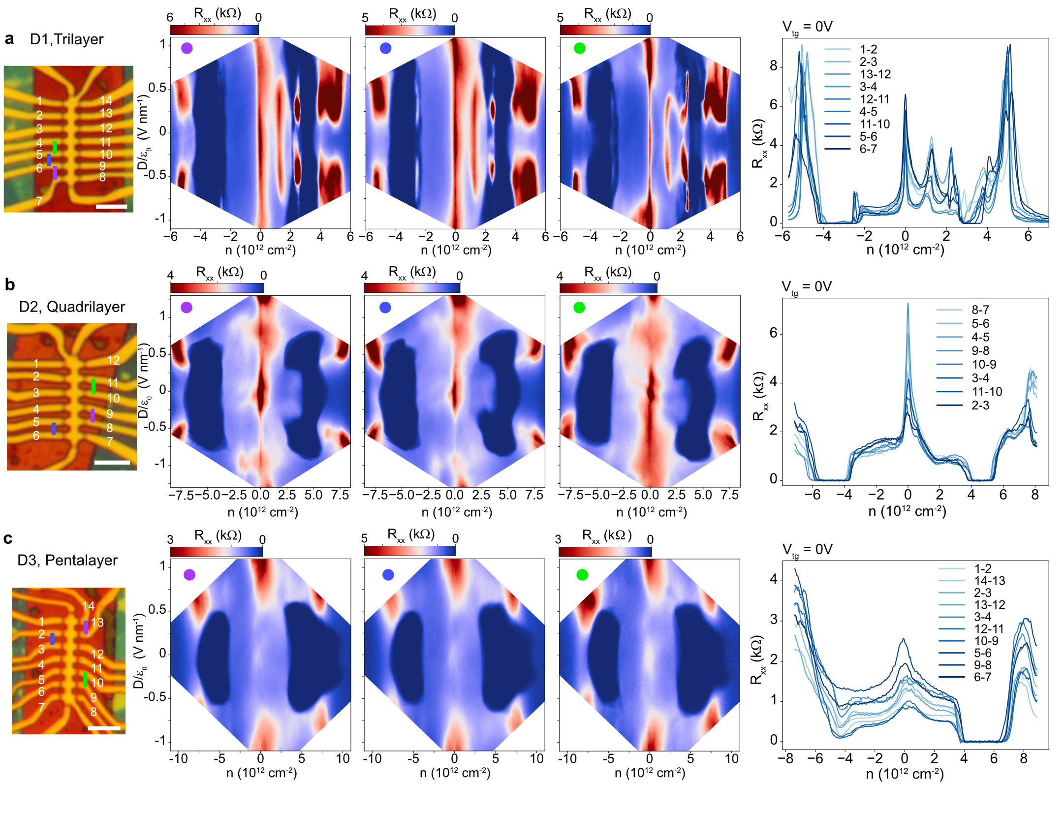
SI Figure 1: Sample uniformity and reproducibility of the results. a–c, Leftmost optical images are D1–D3 mentioned in the main text. The scale bar in each panel corresponds to $5~{}\mu$m. $R_{xx}$ versus density and displacement field ($n$–$D$) plots shown in the middle are obtained from electrodes marked with the corresponding colored lines. The electrodes marked with purple lines were used for measuring $R_{xx}$ in the main text. Rightmost plots are $R_{xx}$ versus carrier density with top-gate voltage fixed at V${}_{\textsubscript{tg}}$ = 0 V. All three devices have a high degree of homogeneity in twist angle with the same superconducting filling range and $|\nu|=4$ carrier density for multiple contacts. The behaviour of superconductivity and other symmetry-breaking features is highly reproducible for different contacts.

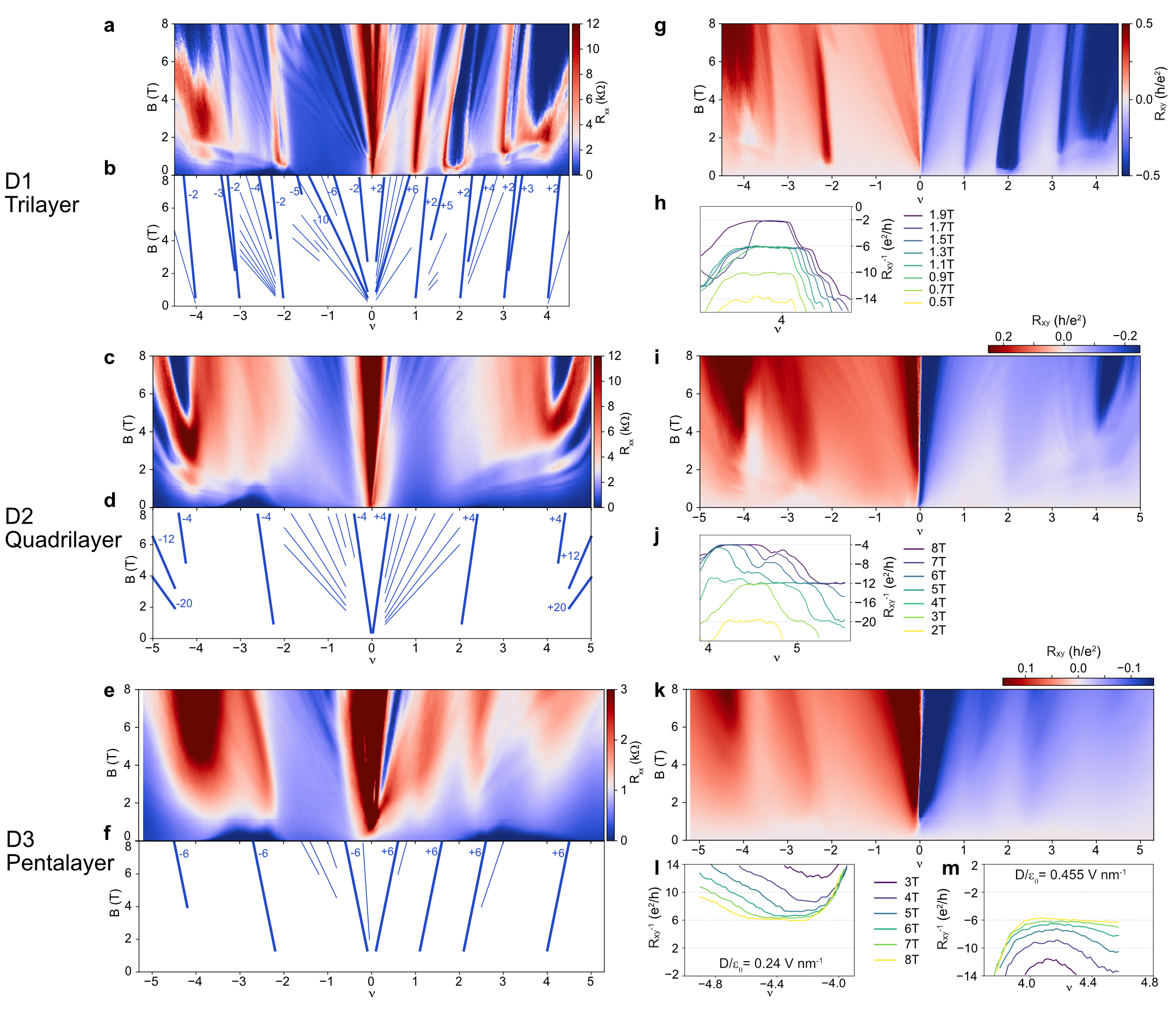
SI Figure 2: Fan diagrams at zero $D$ field and the Hall conductance quantization around $|\nu|=4$. a–f, $R_{xx}$ measured as a function of $B$ field and $\nu$ from trilayer to pentalayer (a, c, e). The main sequences of the fan diagrams are labelled at the bottom of $R_{xx}$ (b, d, f). Landau levels from the dispersive bands are visible as $R_{xx}$ oscillations at low $B$ fields in the fan diagrams. g–m, $R_{xy}$ measured as a function of $B$ field and $\nu$ from trilayer to pentalayer (g, i, k). Below these plots, we show Hall conductance around $|\nu|=4$ (h, j, l, m). The layer number $n$ determines the resulting quantization. Since the dispersive bands of $n$-layer twisted graphene consist of $n-2$ Dirac-like cones (at low energies), the $|\nu|=4$ quantization is therefore expected to follow monolayer graphene sequence ($\pm 2$, $\pm 6$, $\pm 10$,…, $\times e^{2}/h$) multiplied by $n-2$. The plateaus in TTG and TQG clearly show this trend, while in TPG only the first plateau is observed. These observations however confirm the number of layers in each sample.

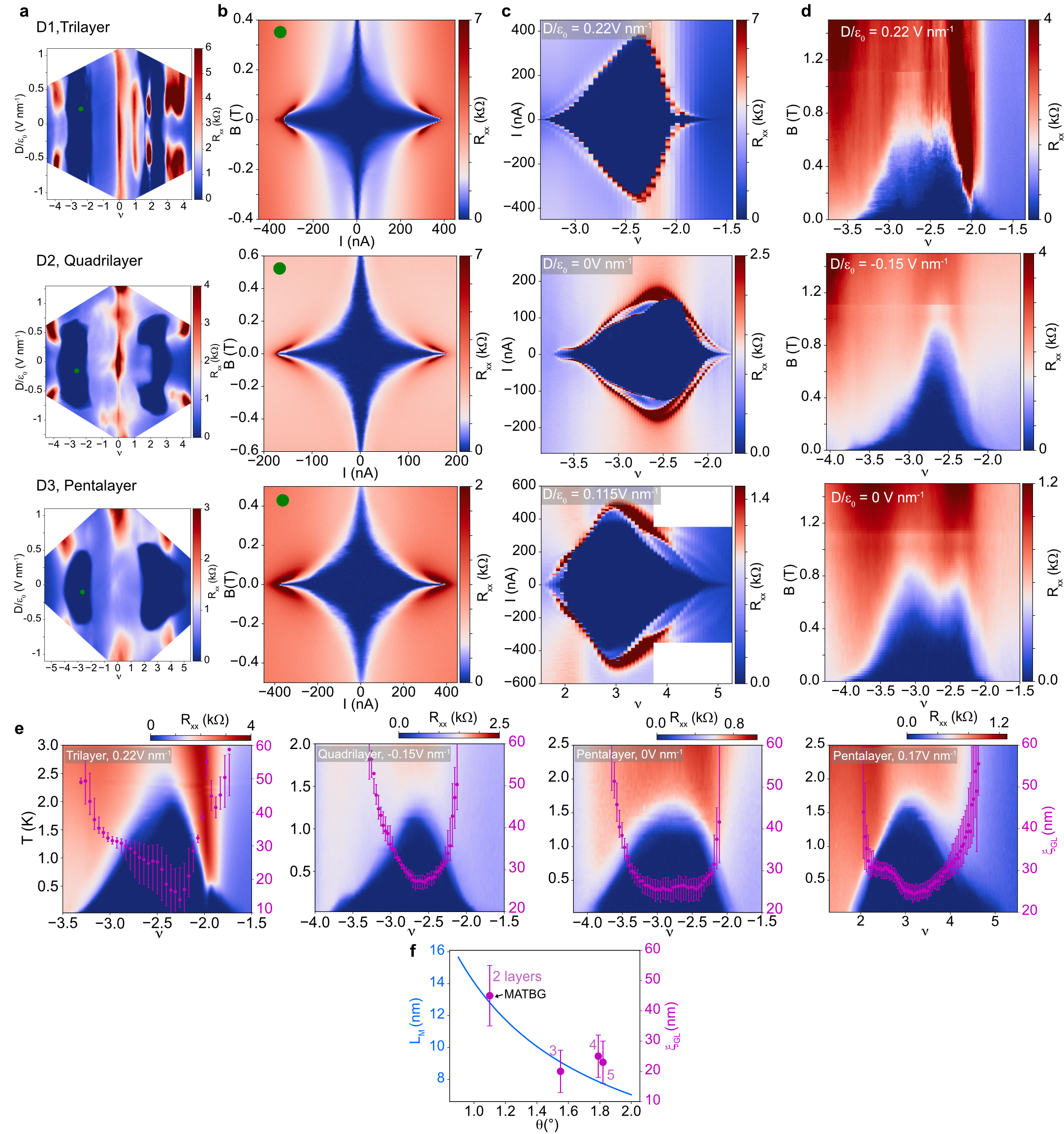
SI Figure 3: Fraunhofer patterns, $I_{c}$, $B_{c}$ and coherence lengths of TTG, TQG and TPG. Column a shows $R_{xx}$ versus $\nu$ and $D$ phase diagrams, and the green dots indicate the positions where the corresponding Fraunhofer interference patterns (b) are measured for D1–D3. Column c shows the critical current $I_{c}$ versus $\nu$ at the optimal $D$ fields for D1–D3. Column d shows $R_{xx}$ versus $\nu$ and $B$ around $\nu=-2$ for D1–D3, highlighting the high critical magnetic fields in these systems. Superconductivity in the twisted graphene multilayers has a higher $B_{c}$ ($\sim 0.8$ T or higher) than in TBG. e, Ginzburg–Landau coherence lengths $\xi_{\mathrm{GL}}$ versus $\nu$ for all three devices around $|\nu|=2$, superimposed on the $R_{xx}$ versus $T$ and $\nu$ plots. f, $\xi_{\mathrm{GL}}$ and moiré wavelength $L_{\mathrm{M}}$ versus twist angle of different layers, suggesting a possible relation between the two length scales.

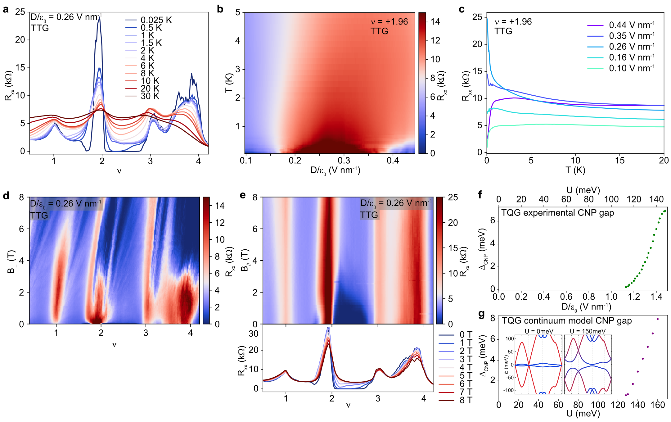
SI Figure 4: Insulating behaviour in TTG and TQG. a, Line cuts of $R_{xx}$ versus $\nu$ for a range of temperatures at $D/\epsilon_{0}=0.26~{}\text{V nm}^{-1}$ on the electron side for TTG. b, $R_{xx}$ versus $D$ and temperature at $\nu=+1.96$ in TTG. c, Line cuts at different $D$ fields from b. Out-of-plane (d) and in-plane (e) $B$ field dependence of $R_{xx}$ versus $\nu$ at $D/\epsilon_{0}=0.26~{}\text{V nm}^{-1}$ in TTG. The $\nu=+2$ correlated insulator is suppressed by both in-plane and out-of-plane $B$ field. f, Experimental charge-neutrality gap of TQG as a function of $D$ field, and g, the continuum-model gap as a function of potential difference $U$. Inset, single-particle band structure of TQG (slightly above the magic angle) at $U=0~{}\text{meV}$ and $150~{}\text{meV}$, respectively. We see a good match between experiment and theory when converting $D$ into $U$ with an empirical factor: $U=0.1\times(n-1)\times 0.33~{}{\rm nm}\times eD$, where $n-1$ is the number of graphene interfaces.

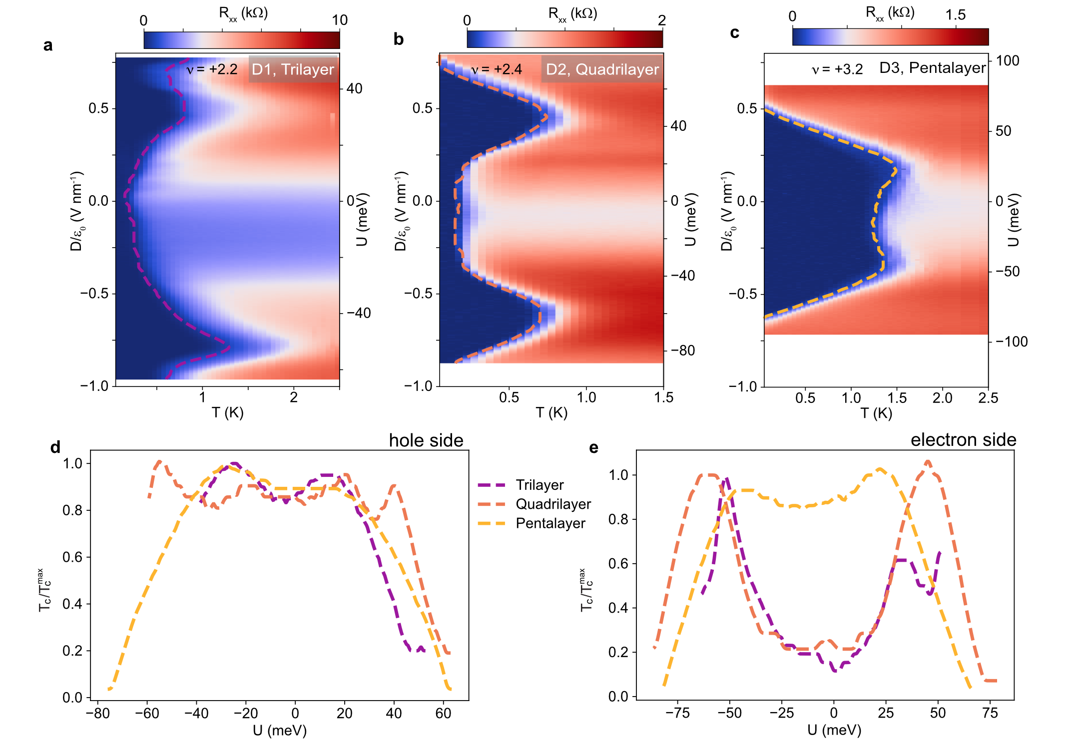
SI Figure 5: Evolution of superconducting critical temperature $T_{c}$ with $D$ field around optimal doping. a–c, $R_{xx}$ as a function of $T$ and $D$ field for D1–D3 at filling factor $\nu=+2.2$, $+2.4$, and $+3.2$, respectively. Superconducting $T_{c}$ is indicated by a dashed line that delineates $10\%$ of the normal state resistance (see section 2 for details). d,e, $T_{c}/T_{c}^{max}$ versus potential energy difference $U$ for TTG, TQG, and TPG around hole-side (d) and electron-side (e) optimal doping, respectively. $U$ is converted from $D$ using $U=0.1\times(n-1)\times 0.33~{}{\rm nm}\times eD$, where $e$ is the electron charge and $n-1$ is the number of graphene interfaces.

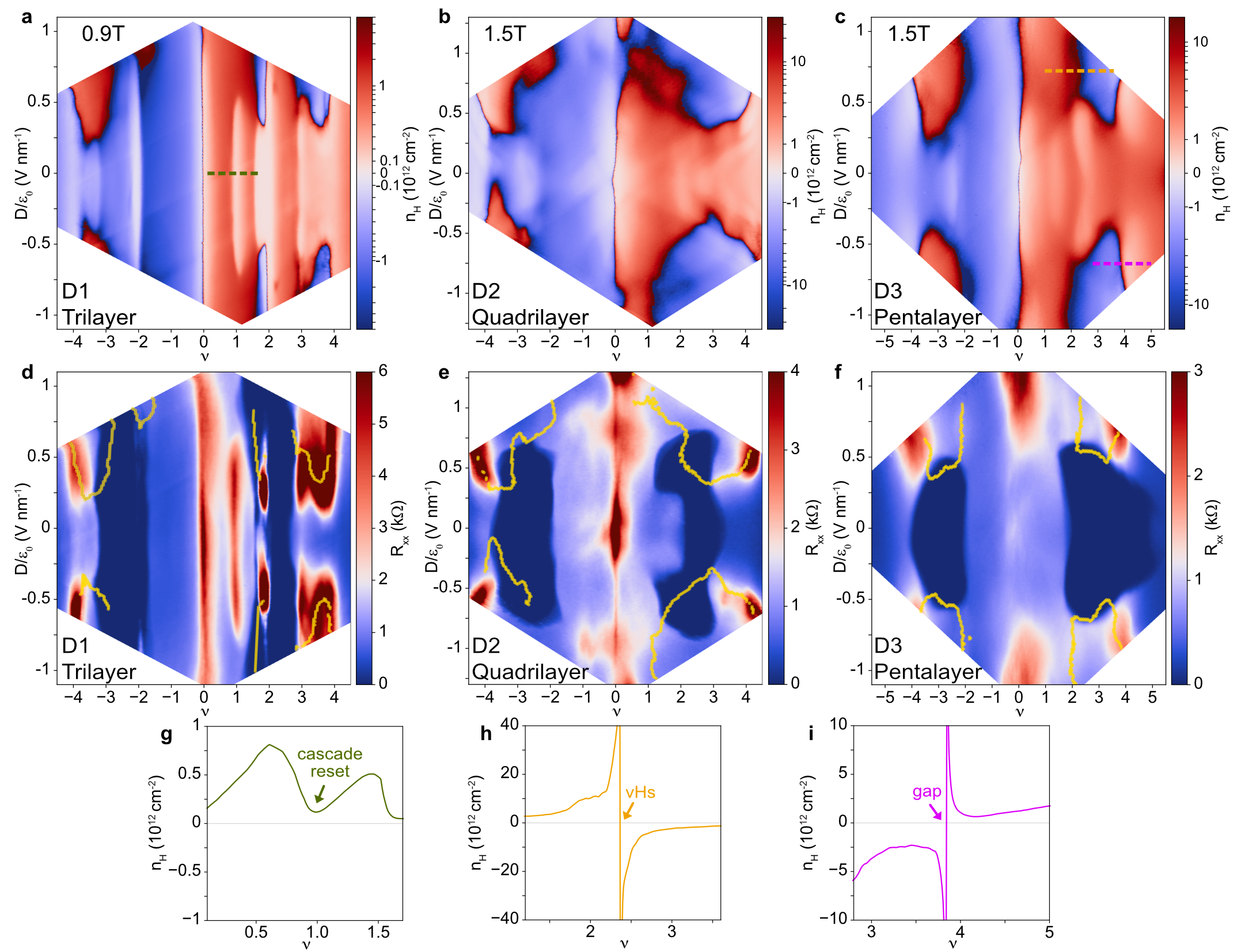
SI Figure 6: Hall density $\nu$–$D$ maps and the positions of vHs/‘gap’ features. a–f, Hall density (a–c) and $R_{xx}$ (d–f) as a function of $\nu$ and $D$ for TTG, TQG, and TPG. Hall density maps are measured at $B=0.9$ T, $1.5$ T, and $1.5$ T, respectively. Yellow lines in d–f track the evolution of vHs/‘gap’ features where Hall density changes sign. g–i, Examples of Hall density near the cascade transition reset (g), the vHs (h), and the ‘gap’ (i) following the definitions in Ref. 10. Filling ranges for the line cuts are marked by the corresponding colored dashed lines in a and c.

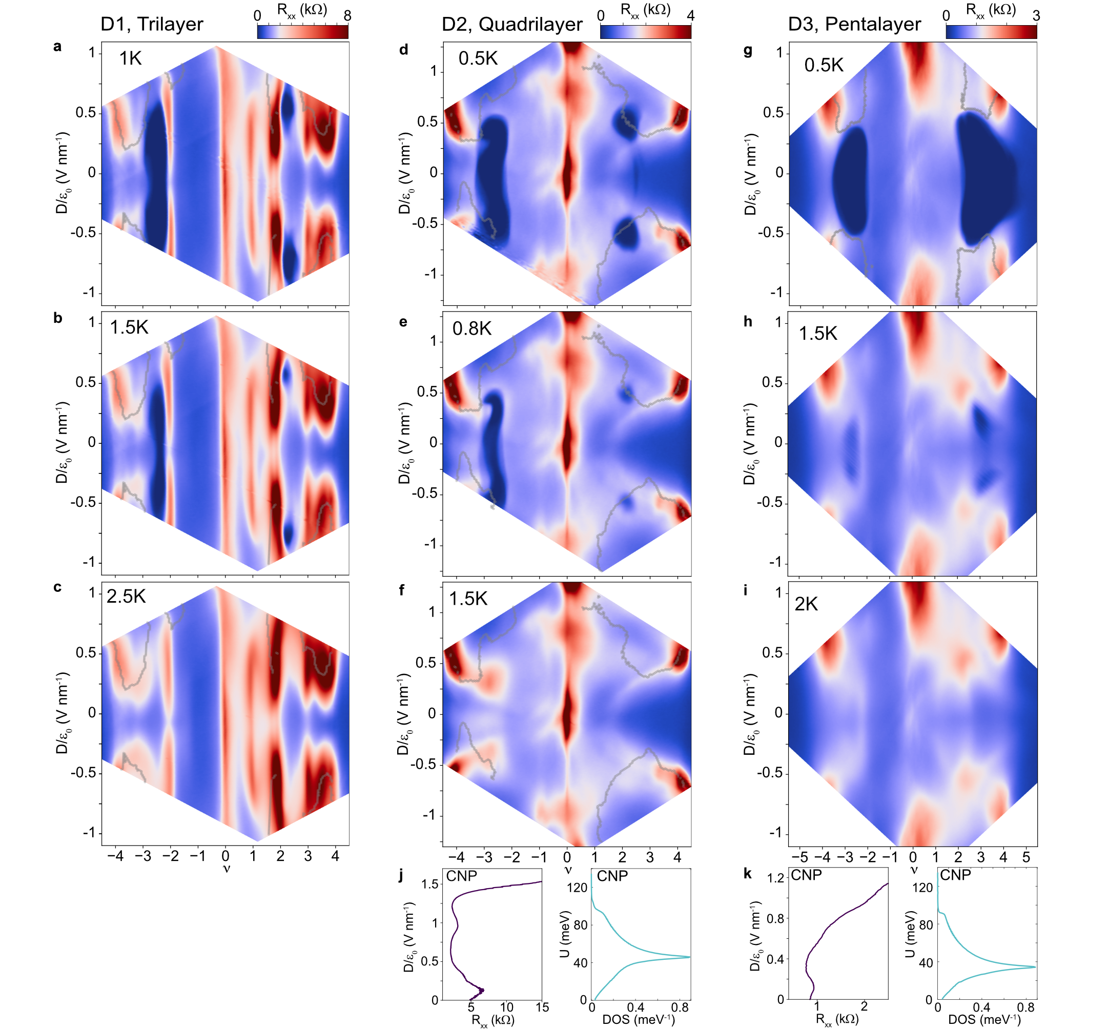
SI Figure 7: $R_{xx}$ as a function of $\nu$ and $D$ at different temperatures. a–i, $R_{xx}$ as a function of $\nu$ and $D$ measured at different temperatures for TTG (a–c), TQG (d–f), and TPG (g–i). Grey lines track the evolution of the vHs/‘gap’ features. j, The plot on the left shows line cut of $R_{xx}$ versus $D$ at charge neutrality for TQG. The plot on the right shows corresponding density of states (DOS) at charge-neutrality point (CNP) calculated using non-interacting continuum model. In the regions where DOS is high, resistance is expected to be low and vice versa. k, Equivalent plots as in j for TPG.

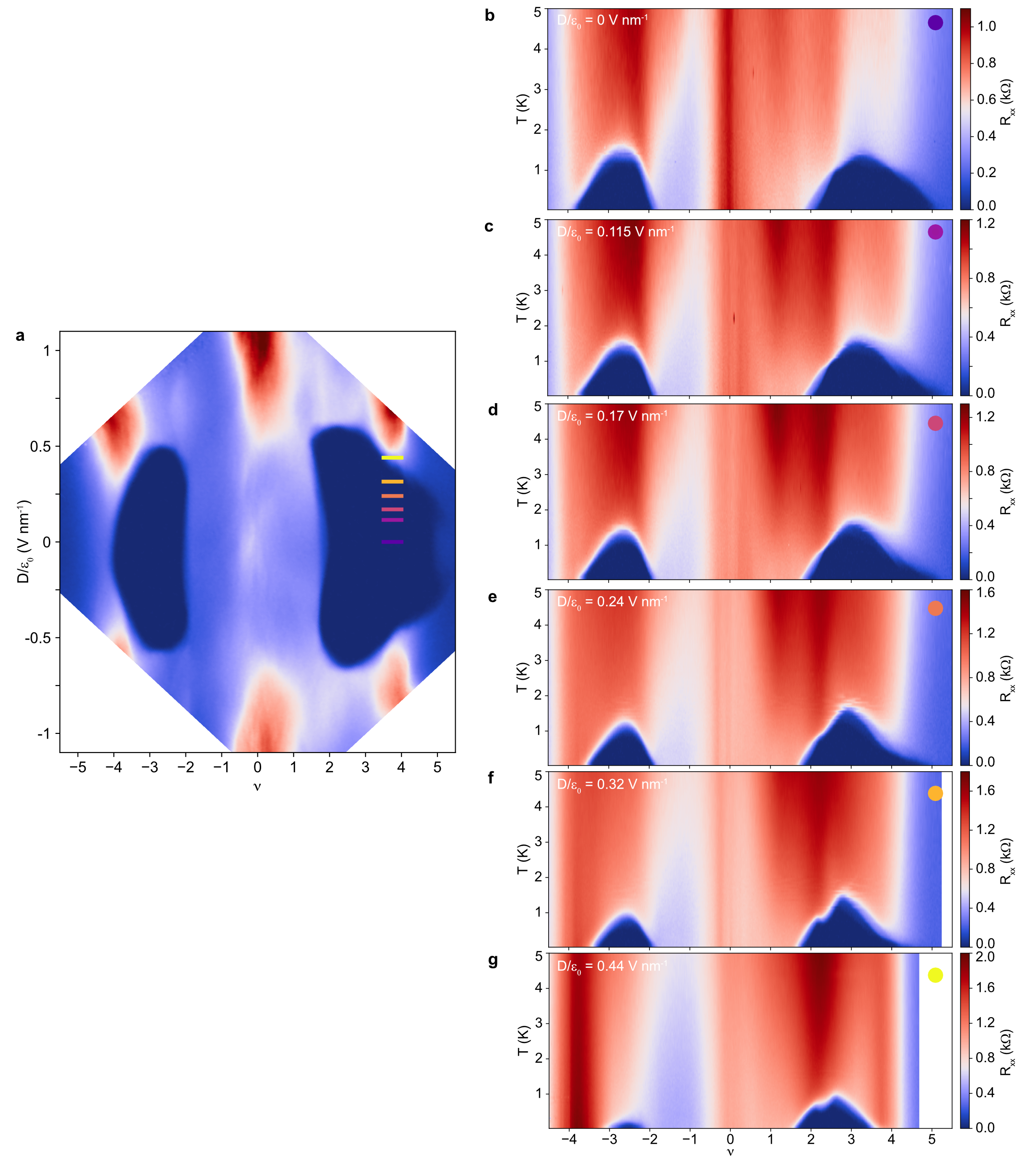
SI Figure 8: Evolution of superconducting $\nu$–$T$ domes with displacement field $D$ in TPG. a, $R_{xx}$ as a function of $\nu$ and $D$ in TPG. b–g, $R_{xx}$ versus $\nu$ and temperature at different $D$ fields, and $D$ fields are marked with colored bars in a.

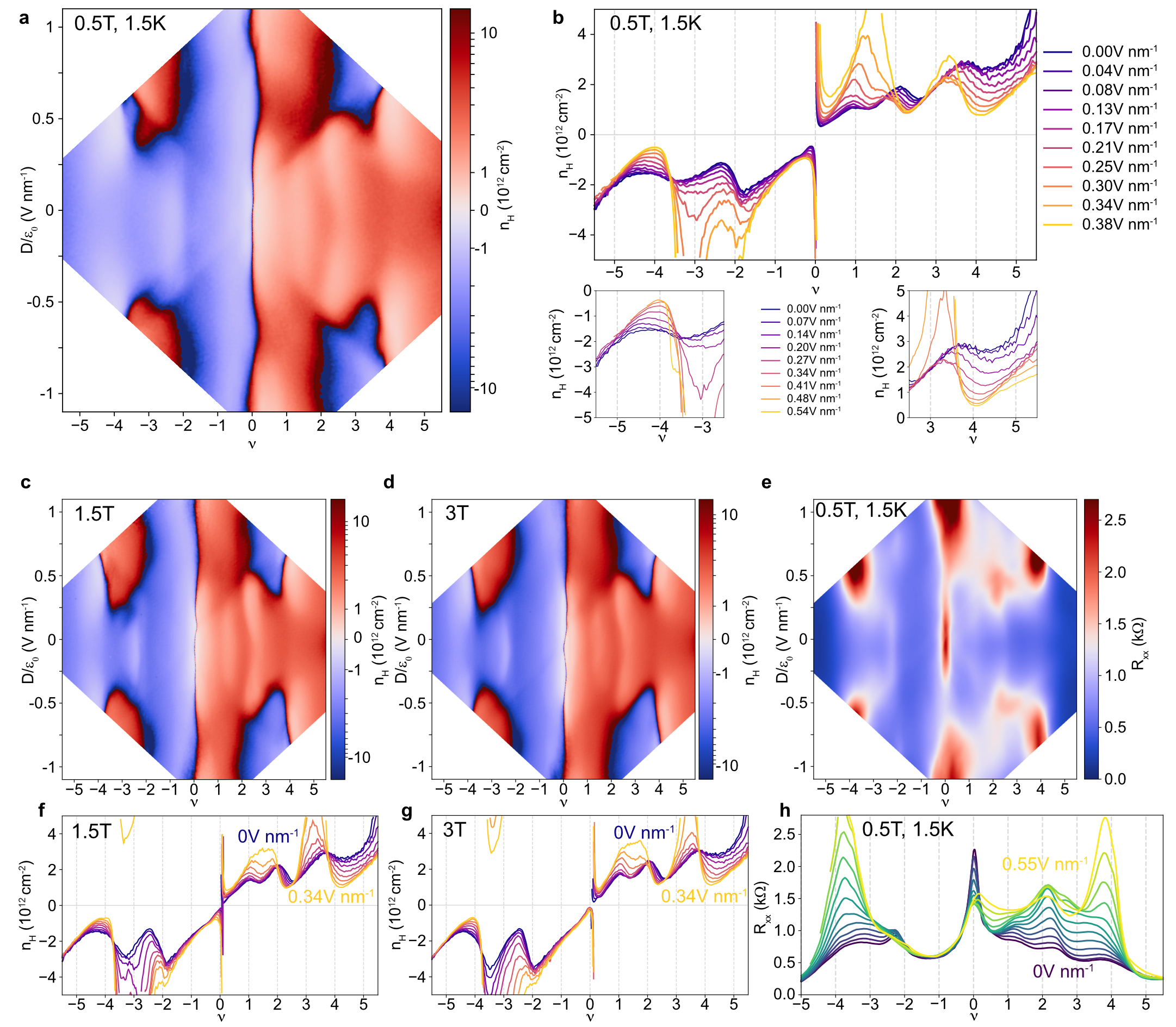
SI Figure 9: Hall density and $R_{xx}$ as a function of $\nu$ and $D$ measured at different $B$ fields in TPG. a, Hall density versus $D$ and $\nu$ at $B=0.5$ T. b, Line cuts from a. Panels below zoom in on the evolution of Hall density resets near $|\nu|=4$. c,d, Hall density versus $D$ and $\nu$ measured at $B=1.5$ T (c) and $3$ T (d), with respective line cuts shown in f and g. e, $R_{xx}$ versus $D$ and $\nu$ measured at $T=1.5$ K, $B=0.5$ T (line cuts are shown in h). From all the above line cuts, Hall density resets and $R_{xx}$ resistive features consistently exist around $\nu=+4$.

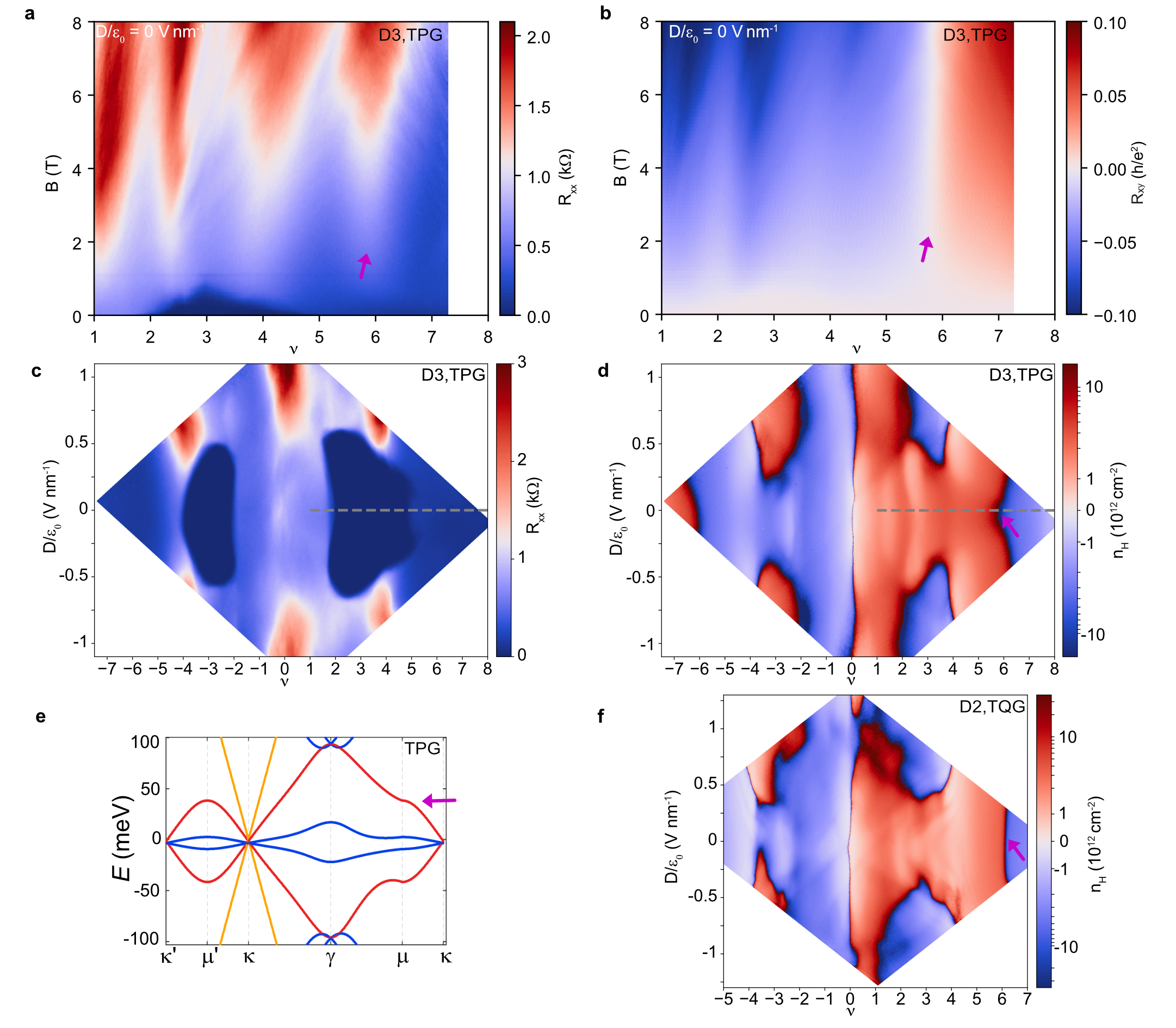
SI Figure 10: Plots in a broader filling factor range and vHs of dispersive TBG-like bands in TPG and TQG. a,b, $R_{xx}$ and $R_{xy}$ as a function of $\nu$ and $B$ field measured at zero $D$ field for TPG. The sign change in $R_{xy}$ around $\nu=+6$ (marked by arrows in a and b) indicates vHs. c,d, $R_{xx}$ (c) and Hall density (d) as a function of $D$ and $\nu$ with gray dashed lines indicating $\nu$ linecuts (at $D=0$) where plots in a and b are taken. e, Band structure of TPG calculated using non-interacting model. Arrow indicates the position where vHs from dispersive TBG-like bands is expected. f, Hall density as a function of $\nu$ and $D$ for TQG. As in TPG, Hall density changes sign near $\nu=+6$ indicating the vHs from dispersive TBG-like bands in TQG.

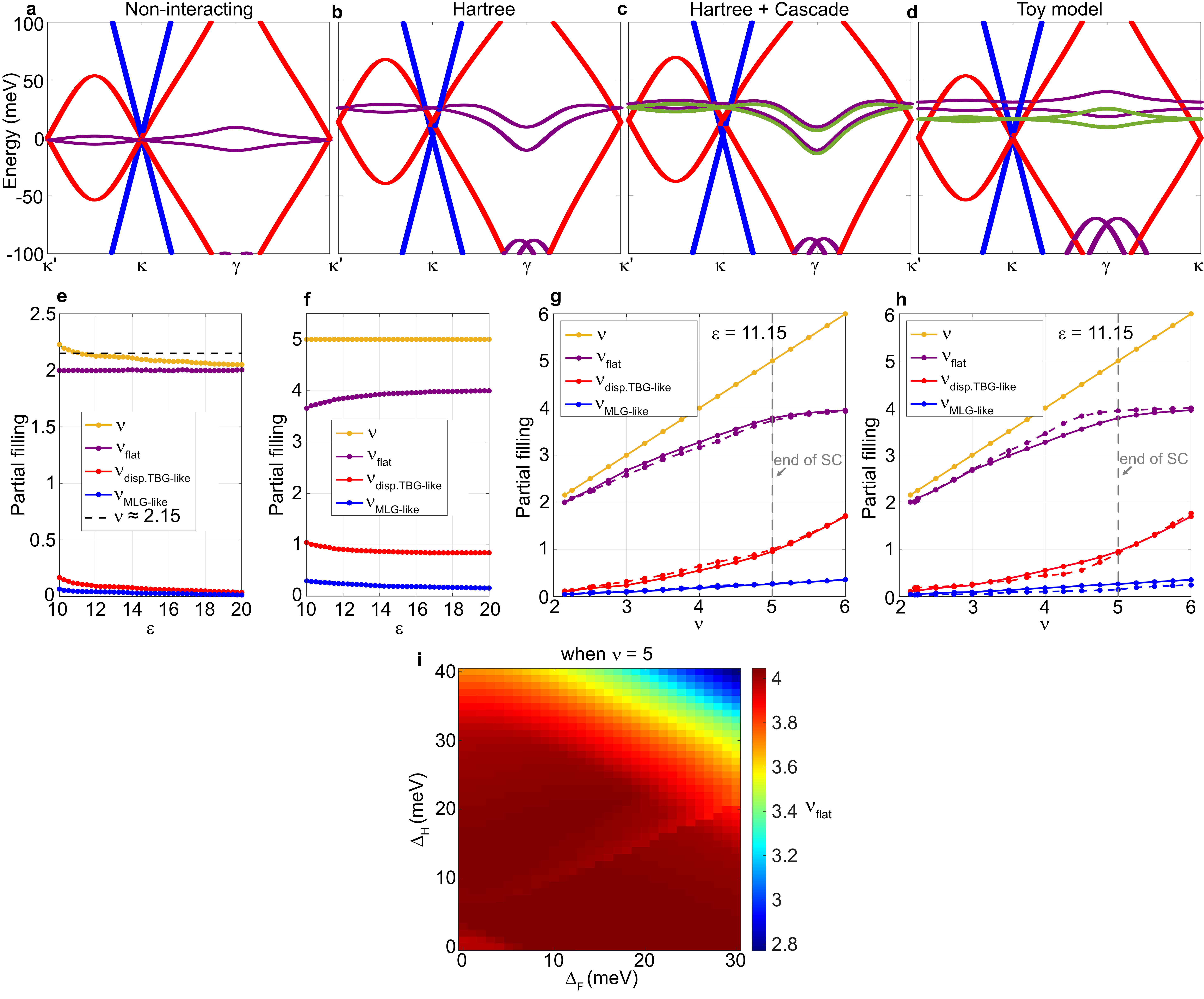
SI Figure 11: The role of interactions in TPG. a-d, Depiction of different approximation schemes used to understand the role of interactions in TPG. Note that the Hartree correction shifts the flat band (purple) up in energy. Cascaded bands in c and d are shown in green. d corresponds to a simple toy model of Hartree and Fock effects characterized by a Hartree shift ($\Delta_{H}$) and a Fock gap ($\Delta_{F}$) (see section 4.5). e,f, Partial filling of each subsystem versus dielectric constant $\epsilon$ for a fixed flat-band filling $\nu_{\mathrm{flat}}=+2$ (e) and a fixed total filling $\nu=+5$ (f), respectively. g, Partial filling of each subsystem versus total filling $\nu$ for a fixed dielectric constant $\epsilon=11.15$. Here, solid (dashed) lines correspond to a cascaded (uncascaded) solution with the cascade solution enabling higher filling of the flat-band subsystem as discussed in the text. h, Similar to g but the solid (dashed) lines correspond to a solution at potential difference $U=0$ meV ($U=34$ meV). i, Filling of the flat-band subsystem as a function of $\Delta_{H}$ and $\Delta_{F}$ at a fixed total filling $\nu=+5$ (see section 4.5).

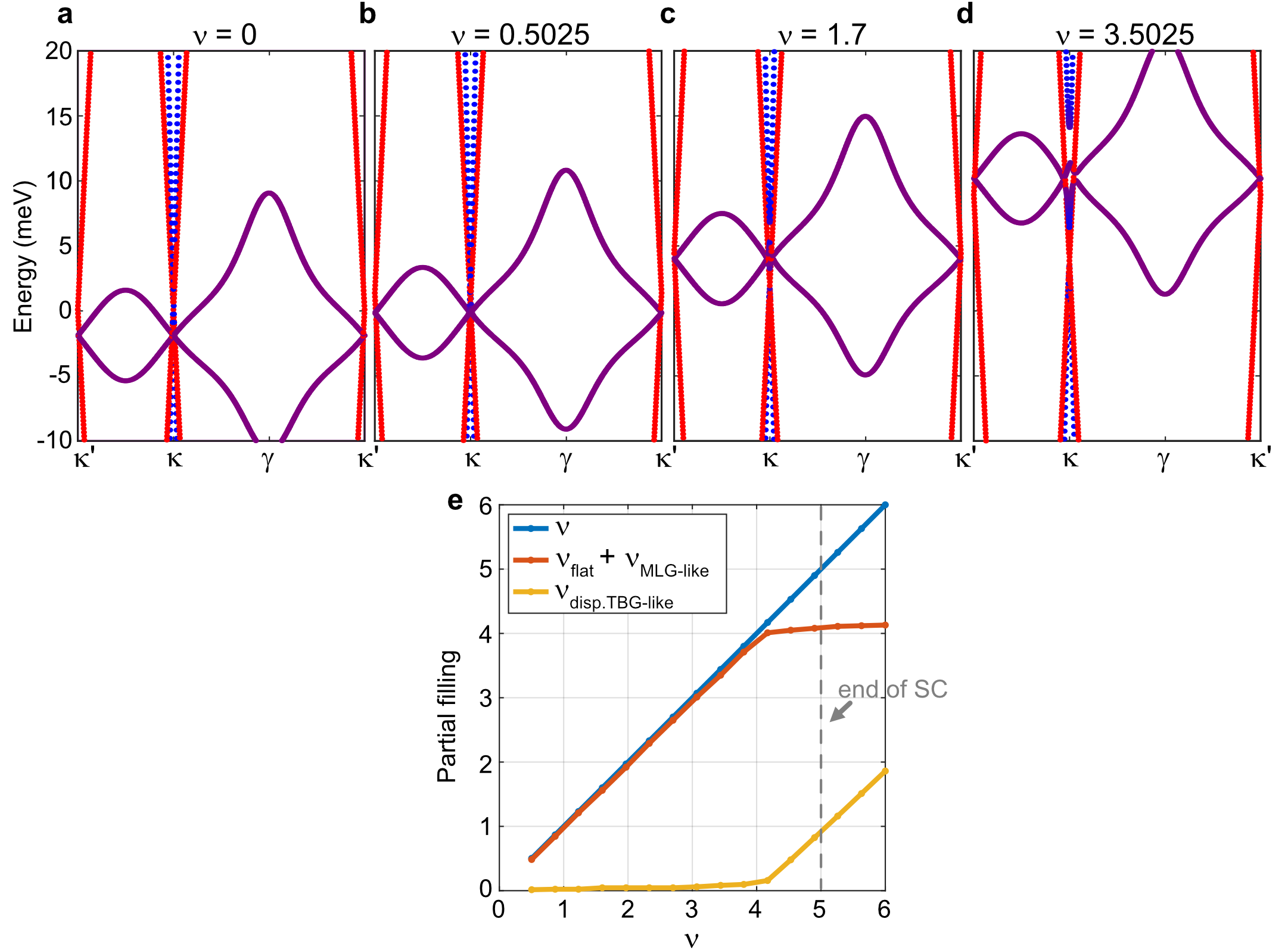
SI Figure 12: The role of interlayer inhomogeneous charge distribution in TPG. a–d, Band structure of TPG at different filling factors with an interlayer inhomogeneous charge distribution. Note that as filling is increased, the flat band is slightly shifted and also hybridizes with the MLG-like band. e, Partial filling of different subsystems as a function of total filling $\nu$ with the effect of interlayer inhomogeneous charge distribution. Note a small charge redistribution between $+2\lesssim\nu\lesssim+5$. Here, flat TBG-like and MLG-like subsystems are plotted together to demonstrate the emergent hybridization.

References

- [1] Cao, Y. et al. Correlated insulator behaviour at half-filling in magic-angle graphene superlattices. Nature 556, 80–84 (2018).
- [2] Serlin, M. et al. Intrinsic quantized anomalous Hall effect in a moiré heterostructure. Science 367, 900–903 (2019).
- [3] Zondiner, U. et al. Cascade of phase transitions and Dirac revivals in magic-angle graphene. Nature 582, 203–208 (2020).
- [4] Choi, Y. et al. Electronic correlations in twisted bilayer graphene near the magic angle. Nature Physics 15, 1174–1180 (2019).
- [5] Wong, D. et al. Cascade of electronic transitions in magic-angle twisted bilayer graphene. Nature 582, 198–202 (2020).
- [6] Choi, Y. et al. Correlation-driven topological phases in magic-angle twisted bilayer graphene. Nature 589, 536–541 (2021).
- [7] Nuckolls, K. P. et al. Strongly correlated Chern insulators in magic-angle twisted bilayer graphene. Nature 588, 610–615 (2020).
- [8] Khalaf, E., Kruchkov, A. J., Tarnopolsky, G. & Vishwanath, A. Magic angle hierarchy in twisted graphene multilayers. Physical Review B 100, 085109 (2019).
- [9] Cao, Y. et al. Unconventional superconductivity in magic-angle graphene superlattices. Nature 556, 43–50 (2018).
- [10] Park, J. M., Cao, Y., Watanabe, K., Taniguchi, T. & Jarillo-Herrero, P. Tunable strongly coupled superconductivity in magic-angle twisted trilayer graphene. Nature 590, 249–255 (2021).
- [11] Hao, Z. et al. Electric field–tunable superconductivity in alternating-twist magic-angle trilayer graphene. Science 371, 1133–1138 (2021).
- [12] Cao, Y., Park, J. M., Watanabe, K., Taniguchi, T. & Jarillo-Herrero, P. Pauli-limit violation and re-entrant superconductivity in moiré graphene. Nature 595, 526–531 (2021).
- [13] Liu, X., Zhang, N. J., Watanabe, K., Taniguchi, T. & Li, J. I. A. Coulomb screening and thermodynamic measurements in magic-angle twisted trilayer graphene. arXiv:2108.03338 [cond-mat] (2021). 2108.03338.
- [14] Arora, H. S. et al. Superconductivity in metallic twisted bilayer graphene stabilized by WSe2. Nature 583, 379–384 (2020).
- [15] Christos, M., Sachdev, S. & Scheurer, M. S. Correlated insulators, semimetals, and superconductivity in twisted trilayer graphene. arXiv:2106.02063 [cond-mat] (2021). 2106.02063.
- [16] Xie, F., Regnault, N., Călugăru, D., Bernevig, B. A. & Lian, B. Twisted symmetric trilayer graphene. II. Projected Hartree-Fock study. Physical Review B 104, 115167 (2021).
- [17] Oh, M. et al. Evidence for unconventional superconductivity in twisted bilayer graphene. arXiv:2109.13944 [cond-mat] (2021). 2109.13944.
- [18] Kim, H. et al. Spectroscopic Signatures of Strong Correlations and Unconventional Superconductivity in Twisted Trilayer Graphene. arXiv:2109.12127 [cond-mat] (2021). 2109.12127.
- [19] Qin, W. & MacDonald, A. H. In-Plane Critical Magnetic Fields in Magic-Angle Twisted Trilayer Graphene. Physical Review Letters 127, 097001 (2021).
- [20] Kopnin, N. B., Heikkilä, T. T. & Volovik, G. E. High-temperature surface superconductivity in topological flat-band systems. Physical Review B 83, 220503 (2011).
- [21] Potasz, P., Xie, M. & MacDonald, A. H. Exact Diagonalization for Magic-Angle Twisted Bilayer Graphene. Physical Review Letters 127, 147203 (2021). 2102.02256.
- [22] Shavit, G., Berg, E., Stern, A. & Oreg, Y. Theory of correlated insulators and superconductivity in twisted bilayer graphene. arXiv:2107.08486 [cond-mat] (2021). 2107.08486.
- [23] Xie, F. et al. Twisted bilayer graphene. VI. An exact diagonalization study at nonzero integer filling. Physical Review B 103, 205416 (2021).
- [24] Ledwith, P. J. et al. TB or not TB? Contrasting properties of twisted bilayer graphene and the alternating twist $n$-layer structures ($n=3, 4, 5, \dots$). arXiv:2111.11060 [cond-mat] (2021). 2111.11060.
- [25] Guinea, F. & Walet, N. R. Electrostatic effects, band distortions, and superconductivity in twisted graphene bilayers. Proceedings of the National Academy of Sciences 115, 13174–13179 (2018).
- [26] Rademaker, L., Abanin, D. A. & Mellado, P. Charge smoothening and band flattening due to Hartree corrections in twisted bilayer graphene. Physical Review B 100, 205114 (2019).
- [27] Goodwin, Z. A. H., Vitale, V., Liang, X., Mostofi, A. A. & Lischner, J. Hartree theory calculations of quasiparticle properties in twisted bilayer graphene. Electronic Structure 2, 034001 (2020). 2004.14784.
- [28] Calderón, M. J. & Bascones, E. Interactions in the 8-orbital model for twisted bilayer graphene. Physical Review B 102, 155149 (2020). 2007.16051.
- [29] Choi, Y. et al. Interaction-driven Band Flattening and Correlated Phases in Twisted Bilayer Graphene. arXiv:2102.02209 [cond-mat] (2021). 2102.02209.
- [30] Fischer, A. et al. Unconventional Superconductivity in Magic-Angle Twisted Trilayer Graphene. arXiv:2104.10176 [cond-mat] (2021). 2104.10176.
- [31] Bi, Z., Yuan, N. F. Q. & Fu, L. Designing flat bands by strain. Physical Review B 100, 035448 (2019).
- [32] Xie, B., Zhang, S. & Liu, J. Alternating twisted mutilayer graphene: Generic partition rules, double flat bands, and orbital magnetoelectric effect. arXiv:2111.06292v1[cond-mat] (2021).
- [33] Zhou, H., Xie, T., Taniguchi, T., Watanabe, K. & Young, A. F. Superconductivity in rhombohedral trilayer graphene. arXiv:2106.07640 [cond-mat] (2021). 2106.07640.
- [34] Zhou, H. et al. Isospin magnetism and spin-triplet superconductivity in Bernal bilayer graphene. arXiv:2110.11317 [cond-mat] (2021). 2110.11317.
- [35] Cao, Y. et al. Superlattice-Induced Insulating States and Valley-Protected Orbits in Twisted Bilayer Graphene. Physical Review Letters 117, 116804 (2016).
- [36] Saito, Y. et al. Isospin Pomeranchuk effect in twisted bilayer graphene. Nature 592, 220–224 (2021).
- [37] Rozen, A. et al. Entropic evidence for a Pomeranchuk effect in magic-angle graphene. Nature 592, 214–219 (2021). 2009.01836.
- [38] Sharpe, A. L. et al. Emergent ferromagnetism near three-quarters filling in twisted bilayer graphene. Science 365, 605–608 (2019).
- [39] Kwan, Y. H. et al. Kekul\’e spiral order at all nonzero integer fillings in twisted bilayer graphene. arXiv:2105.05857 [cond-mat] (2021). 2105.05857.
- [40] Bultinck, N. et al. Ground State and Hidden Symmetry of Magic-Angle Graphene at Even Integer Filling. Physical Review X 10, 031034 (2020). 1911.02045.
- [41] Lian, B. et al. Twisted bilayer graphene. IV. Exact insulator ground states and phase diagram. Physical Review B 103, 205414 (2021).
- [42] Lopes dos Santos, J. M. B., Peres, N. M. R. & Castro Neto, A. H. Graphene Bilayer with a Twist: Electronic Structure. Physical Review Letters 99, 256802 (2007).
- [43] Bistritzer, R. & MacDonald, A. H. Moiré bands in twisted double-layer graphene. Proceedings of the National Academy of Sciences 108, 12233–12237 (2011).
- [44] Carr, S. et al. Ultraheavy and Ultrarelativistic Dirac Quasiparticles in Sandwiched Graphenes. Nano Letters 20, 3030–3038 (2020).
- [45] Călugăru, D. et al. Twisted symmetric trilayer graphene: Single-particle and many-body Hamiltonians and hidden nonlocal symmetries of trilayer moir\’e systems with and without displacement field. Physical Review B 103, 195411 (2021).
- [46] Lei, C., Linhart, L., Qin, W., Libisch, F. & MacDonald, A. H. Mirror symmetry breaking and lateral stacking shifts in twisted trilayer graphene. Physical Review B 104, 035139 (2021).
- [47] Kerelsky, A. et al. Maximized electron interactions at the magic angle in twisted bilayer graphene. Nature 572, 95–100 (2019).
- [48] Xie, Y. et al. Spectroscopic signatures of many-body correlations in magic-angle twisted bilayer graphene. Nature 572, 101–105 (2019).
- [49] Jiang, Y. et al. Charge order and broken rotational symmetry in magic-angle twisted bilayer graphene. Nature 573, 91–95 (2019).
- [50] Cea, T., Walet, N. R. & Guinea, F. Electronic band structure and pinning of Fermi energy to Van Hove singularities in twisted bilayer graphene: A self-consistent approach. Physical Review B 100, 205113 (2019).
- [51] Cea, T. & Guinea, F. Band structure and insulating states driven by Coulomb interaction in twisted bilayer graphene. Physical Review B 102, 045107 (2020).
- [52] Xie, M. & MacDonald, A. H. Weak-field Hall Resistivity and Spin/Valley Flavor Symmetry Breaking in MAtBG. arXiv:2010.07928 [cond-mat] (2020). 2010.07928.
- [53] Liu, S., Khalaf, E., Lee, J. Y. & Vishwanath, A. Nematic topological semimetal and insulator in magic-angle bilayer graphene at charge neutrality. Physical Review Research 3, 013033 (2021).
- [54] Xie, M. & MacDonald, A. H. Nature of the Correlated Insulator States in Twisted Bilayer Graphene. Physical Review Letters 124, 097601 (2020).
- [55] Kang, J. & Vafek, O. Strong Coupling Phases of Partially Filled Twisted Bilayer Graphene Narrow Bands. Physical Review Letters 122, 246401 (2019).
- [56] Guinea, F. Charge distribution and screening in layered graphene systems. Physical Review B 75, 235433 (2007).
- [57] Koshino, M. Interlayer screening effect in graphene multilayers with $ABA$ and $ABC$ stacking. Physical Review B 81, 125304 (2010).