Robustness, Heterogeneous Treatment Effects and Covariate Shifts

Abstract

This paper studies the robustness of estimated policy effects to changes in the distribution of covariates. Robustness to covariate shifts is important, for example, when evaluating the external validity of quasi-experimental results, which are often used as a benchmark for evidence-based policy-making. I propose a novel scalar robustness metric. This metric measures the magnitude of the smallest covariate shift needed to invalidate a claim on the policy effect (for example, $ATE\geq 0$) supported by the quasi-experimental evidence. My metric links the heterogeneity of policy effects and robustness in a flexible, nonparametric way and does not require functional form assumptions. I cast the estimation of the robustness metric as a de-biased GMM problem. This approach guarantees a parametric convergence rate for the robustness metric while allowing for machine learning-based estimators of policy effect heterogeneity (for example, lasso, random forest, boosting, neural nets). I apply my procedure to the Oregon Health Insurance experiment. I study the robustness of policy effects estimates of health-care utilization and financial strain outcomes, relative to a shift in the distribution of context-specific covariates. Such covariates are likely to differ across US states, making quantification of robustness an important exercise for adoption of the insurance policy in states other than Oregon. I find that the effect on outpatient visits is the most robust among the metrics of health-care utilization considered.

Keywords: Robustness, Heterogeneous Treatment Effects, KL divergence, Semiparametric estimation, De-biased GMM, Oregon Health Insurance Experiment

JEL codes: C14, C18, C44, C51, C54, D81, I13

1 Introduction

The guiding principle of evidence-based policy-making is to use experimental and quasi-experimental studies to guide the adoption of policies in various settings. This approach rests on the premise that the quasi-experimental findings are sufficiently robust and generalizable to hold beyond the setting of the quasi-experiment. In practice, this premise does not always hold: there are several examples of policies that, when adopted in non-experimental settings, under-performed their own experimental estimates [Deaton, 2010, Cartwright and Hardie, 2012, Williams, 2020]. In this paper, I argue that quasi-experimental estimates are insufficient to guide policy adoption and should be complemented by a measure of robustness that accounts for how policy recipients differ from the quasi-experimental ones. I develop a robustness metric that quantifies how much the characteristics of the recipients would have to change in order to invalidate the quasi-experimental findings. My metric summarizes the out-of-sample uncertainty that the policy-maker faces regarding the policy recipients’ characteristics. As such, my metric complements traditional summaries of in-sample uncertainty, like the standard errors, which routinely accompany quasi-experimental estimates.

As a motivating example, consider a policy-maker who must decide whether to offer medical insurance coverage to low income households. The policy-maker has access to the experimental estimates of Finkelstein et al. [2012] which suggest that a similar intervention led to higher health-care utilization and reduced financial strain in Oregon. The target population of insurance recipients could differ from the experimental one in Oregon along important dimensions. Our goal is to quantify how robust the experimental findings would be if relevant characteristics of the recipients are allowed to change. In this paper, I provide a solution to this problem by leveraging the policy effect heterogeneity in the experiment.

When policy effects are heterogeneous across sub-populations with different covariate values, quasi-experimental findings are generally not robust to changes in the covariate distributions. In such cases, even small changes in the distribution of the covariates could lead to significant aggregate changes in the policy effects. For example, in the Oregon experiment, subsidized health insurance could benefit sicker patients more than healthier patients. Then, the proportion of recipients with a given pre-existing health status, health habits, and/or co-morbidities may strongly influence the overall effect of the policy. Usually, these types of covariates are exclusively collected in the experimental context and not all of them are accessible in the new policy environment prior to implementation. As a result, the procedures proposed by Hsu et al. [2020] and Hartman [2020] that re-weight sup-population effects by the new environment’s entire set of covariates are generally not feasible. Moreover, the heterogeneity of policy effects across sub-populations with different covariates values can be hard to model. This is because while domain knowledge can help select covariates that are predictive of the heterogeneity of policy effects, it usually cannot pin down a specific functional form for this heterogeneity. Because this heterogeneity links covariate shifts to shifts in the aggregate policy effects, a general approach to robustness must reflect the uncertainty regarding the heterogeneity’s functional form.

My robustness metric avoids the need to specify a functional form for the policy effect heterogeneity, letting it instead be flexibly estimated through the quasi-experimental data. Many popular existing approaches to robustness, like Altonji et al. [2005], Oster [2019] and Cinelli and Hazlett [2020], take advantage of specific functional forms. When designing a robustness metric for distributional changes, relying on functional form assumptions carries important implications for what type of shifts the metric can detect. If the way we measure a shift does not match the way we model heterogeneity, the resulting measure of robustness may be misleading. Consider, for example, measuring the difference between an arbitrary covariate distribution and the quasi-experimental one by reporting the difference in their means. With an unrestricted form for the heterogeneity of policy effects, we can, in general, construct a mean-preserving shift of the covariates’ distribution which invalidates the policy-maker’s claim. For example, in the Oregon experiment, if higher-income recipients have negative effects while lower-income recipients have positive effects, we could construct a mean-preserving spread of the income distribution that induces a negative effect overall. Since their means coincide, such a distribution will have a distance of zero from the experimental covariates. A metric that, in most cases, is equal to zero cannot be very informative for assessing the robustness of quasi-experimental findings. This example suggests that a robustness metric should be general enough to accommodate unknown forms of policy effect heterogeneity. My robustness metric allows for arbitrary forms of policy effects heterogeneity, avoiding the limitations of a parametric model. Despite its generality, my metric is still easy to construct and interpret: a one-number summary of heterogeneity which only depends on quasi-experimental data.

Measuring robustness to covariate shifts requires choosing a distance between an arbitrary distribution of the covariates and the quasi-experimental one. In my approach, I adopt Kullback-Leibler divergence distance (KL distance). The KL distance is a popular choice for sensitivity analysis exercises, appearing recently in Christensen and Connault [2019] who apply it to models defined by moment inequalities and Ho [2020] who uses it in a Bayesian context. It has several advantages in our context. First, it is invariant to smooth transformations of the covariates, hence independent of the covariates’ units. Second, it provides a closed-form expression for the proposed global robustness measure $\delta^{*}$, while other popular robustness approaches, like Broderick et al. [2020] rely on local approximations. Leveraging the closed-form solution I cast estimation of my robustness metric as a GMM problem where the moment equation depends on two components. The first is the observed covariate distribution. The second is a functional parameter capturing the heterogeneity of policy effects, which can be flexibly estimated in the quasi-experimental data.

The heterogeneity of policy effects is often sparse: out of the rich set of covariates available in the quasi-experiment, just a few are needed to approximate it well. When covariate data is even moderately high-dimensional, it can be hard to select which covariates are important ex-ante. Machine-learning estimators, like random forest and boosting, exploit the sparsity to automatically select the key covariates, reducing the need for ad-hoc procedures. Using machine-learning to estimate policy effect heterogeneity is appealing, but it may result in substantial bias in the robustness metric for $\delta^{*}$. To accommodate flexible estimation of policy effect heterogeneity using machine learning methods, I construct a de-biased GMM estimator for my robustness metric $\delta^{*}$. I derive the nonparametric influence function correction for the GMM parameters and leverage the theory in Chernozhukov et al. [2020] to eliminate the first-order effect on $\delta^{*}$. As a result I show that my metric $\delta^{*}$ can be consistently estimated at $\sqrt{n}$-rate under very mild conditions on the first-step estimators of heterogeneity. Under these conditions the heterogeneity functional parameter can be estimated through modern high-dimensional methods like lasso, random forest, boosting and neural nets.

I apply my robustness procedure to study the Oregon health insurance experiment, whose findings have profound implications for public health. I replicate results in Finkelstein et al. [2012] and compute the robustness measure for several outcomes capturing recipients’ heath-care utilization and financial strain. As discussed in Finkelstein et al. [2012] and Finkelstein [2013], the Oregon lottery recipients are older, in worse health, and feature a higher proportion of white individuals compared to the national average. These features invite questions about the robustness of Finkelstein et al. [2012] findings for policy-making in other states. The differences in magnitude and sign between the effects of Medicaid expansion in Oregon and Massachusetts have motivated an effort to reconcile the discrepancy by identifying different populations of beneficiaries in the two states [Kowalski, 2018]. My robustness exercise is complementary to Kowalski [2018]: I compute the smallest change in the distribution of the key covariates identified by Finkelstein [2013], relative to the Oregon benchmark, that can eliminate the positive effect of the lottery on recipients’ health-care utilization and financial strain outcome measures. I find that the increase in outpatients visits is the most robust outcome among the measures of health-care utilization and financial strain.

This paper is also related to a larger strand of the econometric and statistics literature on robustness and sensitivity analysis originally spearheaded by Tukey [1960] and Huber [1965]. Recently, there are many other important but distinct robustness approaches: geared towards external validity [Meager, 2019], [Gechter, 2015], robustness to dropping a percentage of the sample [Broderick et al., 2020], by looking at sub-populations [Jeong and Namkoong, 2020], or with respect to unobservable distributions like in Christensen and Connault [2019], Armstrong and Kolesár [2021], Bonhomme and Weidner [2018], and Antoine and Dovonon [2020]. My contribution complements this tool-set by giving the policy-maker an explicit measure of robustness to shifts in the covariate distributions. There are two reasons to focus on observable characteristics. First, observable characteristics are readily available to the policy-maker and are likely to be of first-level importance when assessing the robustness of quasi-experimental findings. Second, the resulting robustness metric is identified through the quasi-experimental data, limiting the need for bounding or partial identification approaches.

The paper is organized as follows: Section 2 introduces the basic setting and the notion of robustness to changes in the covariate distribution. Section 3 presents the main estimator and its asymptotic properties using the de-biased GMM theory recently developed in Chernozhukov et al. [2020]. Section 4 applies the proposed robustness metric to the Oregon health insurance experiment and reports empirical findings. Section 5 briefly concludes. In the Appendix, I provide all the proofs and discuss multiple extensions.

2 A robustness metric for covariate shifts

In this section, I use the potential outcome framework to explicitly link the heterogeneity of policy effects to the notion of robustness outlined in the introduction. The discussion focuses on the average treatment effect (ATE) as the main aggregate policy effect of interest. The policy-maker wants to assess the robustness of a claim on the magnitude (and/or sign) of the ATE, of the form $ATE\geq\tilde{\tau}$. The claim is true in the quasi-experiment but may no longer be true if covariates changes too much. The idea is to take advantage of the Conditional Average Treatment Effect (CATE), a functional parameter which links sub-population level treatment effects with the ATE. I use CATE to characterize, among the distributions that invalidate the policy-maker’s claim ($ATE\geq{\tau}$), the one that is closest to the distribution of covariates in the quasi-experiment. I label this distribution the least favorable distribution because, among the distributions that invalidate the policy-maker’s claim it is the hardest to distinguish from the covariates in the quasi-experiment. To measure the distance between two covariate distributions I use the Kullback-Leibler divergence distance. The value of the KL distance between the least favorable distribution and the quasi-experimental covariates will be the proposed robustness metric $\delta^{*}$. Any covariate distribution that is closer than $\delta^{*}$ from the quasi-experimental covariates will be guaranteed to satisfy the policy-maker’s claim $(ATE\geq\tilde{\tau})$.

2.1 Notation and Set Up

The policy-maker observes an outcome of interest $Y\in\mathcal{Y}$, a set of covariate measurements $X\in\mathcal{X}$ and a treatment status $D\in\{0,1\}$. I consider two sets of covariates. The first set includes covariates which are exclusively collected in the quasi-experimental data and for which no counterpart exists in census data. For example, in the Oregon health insurance experiment, the recipients’ health status and previous health history is available through survey data but such information may not be accessible through census variables in other settings (perhaps other states). The second set includes covariates for which a counterpart exists in the census data in other states, for example participants’ race and age. To reflect the division of these two covariate types, $X$ could be partitioned into two sets: $X=X_{c}\cup X_{e}$ denoting census covariates and quasi-experiment specific covariates respectively. All variables in $X$ will be used to estimate the treatment effect heterogeneity in the quasi-experiment, which is the functional parameter needed to compute the robustness metric. The details are introduced in Section 2.3. If the policy-maker had access to observations on $X_{c}$ in both the quasi-experiment and in the setting where the policy is to be adopted, my robustness metric can be modified to account for this additional information. To lighten the notation, in the main text I consider $X=X_{e}$ and discuss how to include $X_{c}$ in the Appendix.

Now I introduce the notation to discuss changes in the distribution of the covariates. I use $F_{X}$ to denote the distribution of the covariates in the quasi-experiment and and $P_{X}$ to denote its associated probability measure. The propensity score is defined as $\pi(x)=P_{X}(D=1|X=x)$. Following the traditional potential outcome framework, I denote $Y_{d}$ for $d=\{0,1\}$, the potential outcomes under treated and control status when the distribution of the covariates follows $F_{X}$. For example, in the Oregon experiment, $Y_{1}$ may represent the financial strain of a recipient if they receive insurance coverage while $Y_{0}$ represents the financial strain of the same recipient if they do not receive insurance coverage. In principle the distribution of the potential outcomes depends on the distribution of the covariates. To reflect this, I use $Y_{d}$ and $Y^{\prime}_{d}$ to denote the potential outcomes when the distribution of the covariates follows $F_{X}$ and $F^{\prime}_{X}$ respectively. Finally, for any random variable $W$, $\mathcal{W}$ denotes its support.

The parameter of interest for the policy-maker is the $ATE:=\mathbb{E}[Y_{1}-Y_{0}]$. The Conditional Average Treatment Effect (CATE) defined by $\tau(x):=CATE(x)=\mathbb{E}[Y_{1}-Y_{0}|X=x]$ captures how the average treatment effect changes across sub-populations with covariate value $X=x$. Under unconfounded-ness (Assumption 1 i) below), $\tau(x)$ is nonparametrically identified by $\mathbb{E}[Y|D=1,X=x]-\mathbb{E}[Y|D=0,X=x]$ in the quasi-experiment [Imbens and Rubin, 2015].

Assumption 1.

Unconfounded-ness & Overlap

i) $Y_{1},Y_{0}\mathrel{\text{\scalebox{1.07}{$\perp\mkern-10.0mu\perp$}}}D|X$.
ii) For all $x\in\mathcal{X}$ we have $0<\epsilon\leq\pi(x)\leq 1-\epsilon<1$

In the case of a randomized control trial, for example when treatment assignment is completely randomized or is randomized conditional on covariates, Assumption 1 holds by design. In the case of quasi-experimental studies Assumption 1 i) requires the researcher to carefully evaluate the selection mechanism that governs program participation. Assumption 1 ii) is strict overlap. While strict overlap is not a necessary condition for identification, it will be important in the estimation of the robustness metric in Section 3.

In this paper, the goal is to study the robustness of claims concerning the ATE with respect to changes in the distribution of the covariates. Because the ATE is obtained by averaging $\tau(x)$ with weights proportional to $F_{X}$ we have the following map between the covariate distributions and the ATE:

$$ATE:F_{X}\mapsto\int_{\mathcal{X}}\tau_{F_{X}}(x)dF_{X}(x)$$ (1)

The subscript $F_{X}$ on $\tau(x)$ indicates that, in general, it’s possible that the functional form of CATE depends on $F_{X}$. In this case, a change in the distribution of the covariates would effect the magnitude of ATE through two channels: a direct effect thorough the weights of $F_{X}$ and an indirect effect through changing the functional form of $\tau_{F_{X}}(x)$. In this paper, I introduce the covariate shift assumption to eliminate the indirect effect.

Assumption 2.

(Covariate Shift) Let $X^{\prime}$ denote the covariates in the new environment. Then:

1. $F_{Y_{d}^{\prime}|X^{\prime}}(y|x)=F_{Y_{d}|X}(y|x)$ for $d=\{0,1\}$, for all $x\in\mathcal{X}$ and $y\in\mathcal{Y}_{d}$ and all distributions of $X^{\prime}$.

2. $\mathcal{X}^{\prime}\subseteq\mathcal{X}$

Assumption 2 i) says that the causal link between the treatment variable $D$ and the potential outcomes of interest $Y_{1}$ and $Y_{0}$ does not depend on the distribution of the observables. One could think of Assumption 2 as analogous to a policy invariance condition where the invariance in this case is with respect to the distribution of covariates.

Assumption 2 ii) says the support of the covariates in the new environments is contained in the support of the baseline environment. In practice, this limits the extrapolation to environments for which any value of the covariates could have been observed in the quasi-experimental setting as well. Because Assumption 2 guarantees that $\tau_{F_{X}}(x)$, the CATE, does not vary when $F_{X}$ is replaced by any other distribution $F_{X^{\prime}}$ it is not necessary to index $\tau(x)$ with $F_{X}$. Then, the link between $F_{X}$ and $ATE$ reduces to integration against a fixed $\tau(x)$:

$$ATE:F_{X}\mapsto\int_{\mathcal{X}}\tau(x)dF_{X}(x)$$ (2)

To emphasize the dependence of the $ATE$ on an arbitrary distribution of the covariates $F_{X}$, I occasionally write $ATE(F_{X})$. Before presenting the general framework I give perhaps the simplest nontrivial example of a robustness exercise with respect to the distribution of the covariates.

Example 1.

Consider a binary covariate $X=\{0,1\}$. $D$ is randomly assigned, trivially satisfying Assumption 1. By unconfounded-ness, $\mathbb{E}[Y_{1}|x=0],\mathbb{E}[Y_{0}|x=0],\mathbb{E}[Y_{1}|x=1],\mathbb{E}[Y_{0}|x=1]$ can all be identified. Consequently, the average treatment effect for the sub-populations $x=0$ and $x=1$, denoted $\tau(0)$ and $\tau(1)$ are also identified. Because $X$ is Bernoulli, any distribution on $\{0,1\}$ is fully described by $P_{X}(x=1)=p_{1}$ so automatically $P_{X}(x=0)=1-p_{1}$. Suppose that, in the experiment $ATE\geq 0$. Note that:

$$ATE(F_{X}) =\mathbb{E}[Y_{1}|x=0]\cdot(1-p_{1})+\mathbb{E}[Y_{1}|x=1]\cdot p_{1}$$

$$-\mathbb{E}[Y_{0}|x=0]\cdot(1-p_{1})-\mathbb{E}[Y_{0}|x=1]\cdot p_{1}$$

$$=(\mathbb{E}[Y_{1}|x=0]-\mathbb{E}[Y_{0}|x=0])\cdot(1-p_{1})+(\mathbb{E}[Y_{1}|x=1]-\mathbb{E}[Y_{0}|x=1])\cdot p_{1}$$

$$=\tau(0)\cdot(1-p_{1})+\tau(1)\cdot p_{1}.$$

A shift in the covariate distribution is simply a shift in the parameter $p_{1}$. Assume the treatment effects are sufficiently heterogeneous, namely $\tau(1)>0>\tau(0)$ so one group has positive effects from treatment and the other group has negative effects. What is the closest covariate distribution that invalidates the claim $ATE\geq 0$?

It suffices to find the weights on $x=0,x=1$ such that the ATE is 0. Expressing it in terms of $p_{1}$:

$$\tau(0)\cdot(1-p_{1}^{*})+\tau(1)\cdot p_{1}^{*}=0$$

A solution is given by:

$$p_{1}^{*}=\frac{-\tau(0)}{\tau(1)-\tau(0)}\in[0,1]$$

so the distance $|p_{1}^{*}-p_{1}|=|\frac{-\tau(0)}{\tau(1)-\tau(0)}-p_{1}|$ is largest shift in the covariates that still guarantees that the claim $ATE\geq 0$ holds.

Under what conditions we are always guaranteed to find a solution like $p_{1}^{*}$ above? Is it unique? Can we always characterize the distance between $p_{1}^{*}$ and $p_{1}$? If the space $\mathcal{X}$ is not discrete, a probability distribution on $\mathcal{X}$ cannot be described by a finite dimensional parameter without restricting the class of probability distributions on $\mathcal{X}$. How should one measure the distance between two distributions in general?

I start from this last question by introducing a notion of distance that does not require any parametric restriction on probability distributions. Here I introduce the KL-divergence distance:

Definition 2 (KL-divergence).

Consider the $KL$-divergence between two distributions $F_{X}$ and $F_{X}^{\prime}$ given by:

$$D_{KL}(F_{X}^{\prime}||F_{X}):=\int_{\mathcal{X}}\log\left(\frac{dF_{X}^{\prime}}{dF_{X}}(x)\right)\frac{dF_{X}^{\prime}}{dF_{X}}(x)dF_{X}(x)$$ (3)

where $\frac{dF_{X}^{\prime}}{dF_{X}}$ is the Radon-Nikodym derivative of the distribution $F_{X}^{\prime}$ with respect to the experimental distribution $F_{X}$, provided that $P_{X}^{\prime}\ll P_{X}$ for the respective probability measures.

There are several advantages to using the KL divergence to measure the distance between probability distributions: it is nonparametric, it has useful invariance properties and it delivers a closed form solution for the policy-maker’s robustness problem introduced below. Both Ho [2020] and Christensen and Connault [2019] use the KL divergence to measure the distance between probability distributions in different contexts. Appendix D discusses in detail how to use convex analysis to obtain a closed form solution for the policy-maker’s robustness problem.

2.2 The policy-maker’s problem: quantifying robustness

After isolating the link between the ATE and the distribution of covariates and choosing a distance measure between probability distributions, we can formalize the policy-maker’s robustness problem. Consider the claim given by $ATE\geq\tilde{\tau}$: the $ATE$ is larger than a desired threshold $\tilde{\tau}$. The sign of the inequality is without loss of generality, as claims of the type $ATE\leq\tilde{\tau}$ can be accommodated with an equivalent treatment. The threshold $\tilde{\tau}$ captures a minimal desirable aggregate effect that would make the intervention viable for the policy-maker. It could capture the average cost for the roll-out of the intervention or the value of ATE for a competing policy. In Example 1, $\tilde{\tau}$ was fixed at 0. The policy-maker is interested in the smallest shift from the quasi-experimental distribution, $F_{X}$, such that the claim $ATE\geq\tilde{\tau}$ is invalidated. Recall $\tau(x)=CATE(x)$. Formally the policy-maker wants to solve the following problem:

$$\inf_{dF_{X}^{\prime}:\ dF_{X}^{\prime}\ll dF_{X};dF_{X}^{\prime}(\mathcal{X})=1} D_{KL}(F_{X}^{\prime}||F_{X})$$ (4)

$$s.t.\ \int_{\mathcal{X}}\tau(x)dF_{X}^{\prime}(x)\leq\tilde{\tau}\$$ (5)

The optimization problem in Equation (4) searches across all distributions of the covariates that invalidate the policy-maker’s claim $ATE\geq\tilde{\tau}$ (notice that the ATE for all the distributions in Equation (5) is constrained to be less than $\tilde{\tau}$) and selects, if they exist, the one(s) that are closest to the quasi-experimental distribution $F_{X}$, according to the KL distance in Equation (4). Notice also that $\tau(x)$ in Equation (5) is not indexed by $F_{X}^{\prime}$ because of the covariate shift assumption (Assumption 2). Here, the class of probability measures for the covariates is restricted to be absolutely continuous w.r.t the quasi-experimental measure $dF_{X}$ but no other restriction is imposed: the class of distributions is still nonparametric. Absolute continuity does restrict the distributions $F_{X}^{\prime}$ to be supported on $\mathcal{X}$. While it may appear as an unnecessary restriction, I view it as a very reasonable requirement: the feasible distributions in Equation (5) cannot put mass on a sub-population $X=x$ that could not theoretically be observed in the quasi-experimental setting. Clearly, treatment effect values for sub-populations with $X=x$ that can never be observed can lead to arbitrarily large average effects and the robustness exercise would not be very informative. We are now ready to define the least favorable distribution and the robustness metric.

Definition 3.

i) The least favorable distribution set $\{F_{X}^{*}\}$ is given by the expression below:

$$\{F_{X}^{*}\}= \arg\min_{P_{X}^{\prime}:\ P_{X}^{\prime}\ll P_{X};P_{X}^{\prime}(\mathcal{X})=1}D_{KL}(F_{X}^{\prime}||F_{X})$$ (6)

$$s.t.\ \int_{\mathcal{X}}\tau(x)dF_{X}^{\prime}(x)\leq\tilde{\tau}$$

where the set in Equation (6) is allowed to be the empty set.
ii) For a given $\tilde{\tau}\in\mathbb{R}$ the robustness metric $\delta^{*}(\tilde{\tau})$ is given by:

$$\delta^{*}(\tilde{\tau})=D_{KL}(F_{X}^{*}||F_{X}).$$ (7)

The minimizer of Equation (4) is the least favorable distribution, the closest distribution of the covariates that invalidates the target claim. I define the KL-distance between the experimental distribution and the least favorable distribution as my metric $\delta^{*}(\tilde{\tau})$ which quantifies the robustness of the claim $ATE\geq\tilde{\tau}$. Observe that, if the quasi-experimental ATE satisfies the constraint in Equation (5), then we can always choose the least favorable distribution to be the quasi-experimental one, namely $F_{X}^{*}=F_{X}$ since it’s feasible and $D_{KL}(F_{X}^{*}||F_{X})=0$. In words this means that the policy-maker’s claim is already invalidated in the quasi-experiment. The problem is non-trivial when the $ATE(F_{X})>\tilde{\tau}$ condition is satisfied for the quasi-experimental distribution $F_{X}$. In such a case, the quasi-experimental distribution $F_{X}$ is excluded from the feasible set of Equation (5). As a result, the value of $D_{KL}(F_{X}^{*}||F_{X})$ in Equation (4) must be strictly positive. Notice that, in Example 1, we imposed the requirement that the $ATE(p_{1})$ in the experiment was larger than 0, to guarantee that the problem was indeed non-trivial.

If $\mathcal{X}$ is a set containing finitely many elements, the covariate distribution is discrete. In practice, there are many empirical applications in which covariates of interest are either discrete or have been discretized for privacy reasons. Any grouping of a continuous variables in finitely many classes, gives rise to discrete distribution. For example, in the Oregon experiment, the recipients income may have been discretized into income groups. When the covariates space is discrete, we can get an important geometric insight in the structure of the robustness problem as formulated by Equations (4) and (5). The example below illustrates the case where $\mathcal{X}$ contains only 3 points. In this case, a probability distribution on $\mathcal{X}$ can be parametrized by 2 parameters and there is convenient visual representation of the robustness problem contained in Equations (4) and (5).

Example 4.

Consider the case $\mathcal{X}=\{x_{1},x_{2},x_{3}\}$ each value representing an income bin: high, medium and low respectively. Here the experimental distribution is represented by a triplet $(p_{1},p_{2},p_{3})$. Because $p_{1}+p_{2}+p_{3}=1$ the whole space of probability distributions on $\mathcal{X}$ is 2-dimensional: it suffices to choose $p_{1}$ and $p_{2}$ to fully characterize a distribution. Suppose that conditional treatment effects are highest for lower income participants and are lowest for high income participants: $\tau(x_{1})=1,\tau(x_{2})=2,\tau(x_{3})=3$. The average cost of roll-out is equal to $\tilde{\tau}=1.8$. The claim is $ATE\geq\tilde{\tau}$ meaning that the ATE should be higher than average cost. In the experiment ATE is equal to $2.4>1.8$ which satisfies the claim.

The policy-maker’s robustness problem in Example 4 is depicted in Figure 1. Since the functions in Equations (4) and (5) are differentiable in $p_{1}$ and $p_{2}$ the finite dimensional problem could be easily solved through the standard Karush-Kuhn-Tucker conditions. The level sets of the KL distance, the feasible set and the least favorable distribution are all indicated in Figure 1. The KL level set associated to $\delta^{*}(\tilde{\tau})$ is highlighted by a green contour. It includes the set of covariate distributions that are guaranteed to satisfy the policy-maker’s claim. This region is conservative, in the sense that there exist covariate distributions that satisfy the policy-maker’s claim but fall outside of the green contour. This feature reflects the definition of robustness as a minimization problem in Equations (4) and (5).

When $\mathcal{X}$ is not discrete, a representation like Figure 1 may not be possible. Nonetheless one can still show that, given some conditions, a solution for $F_{X}^{*}$ like the one in Figure 1 always exists, is unique, and can be characterized by a closed form expression, with virtually little difference from the finite dimensional case. This result also guarantees that the robustness metric $\delta^{*}(\tilde{\tau})$ is well defined for a wide range of $\tilde{\tau}$ values.

Figure 1: The triangle represents the collection of all arbitrary probability distribution triplets $(p_{1},p_{2},p_{3})$ on the discrete set $(x_{1},x_{2},x_{3})$ represented in barycentric coordinates. P denotes the experimental distribution, given by $(0.2,0.2,0.6)$. The $CATE(x_{1},x_{2},x_{3})=(1,2,3)$ so the conditional treatment effect is greater in the highest income group. The yellow shaded region is the feasible set: the collection of covariate distributions with an $ATE\leq 1.8$, which invalidate the policy-maker’s claim. The solid yellow line is the boundary of the feasible set. The contour lines from blue to red represent the level sets of the KL distance of any distribution in the triangle with respect to the experimental distribution P (bluer indicates a lower value for the KL divergence). The distribution $P^{*}=(0.491,0.218,0.291)$ is the least favorable distribution. It is the minimizer of the KL divergence, subject to the feasibility constraint (it lies on the orange line). The green boundary is the level set of KL that corresponds to $\delta^{*}\approx 0.296$. Any distribution closer than $\delta^{*}$, within the green boundary is guaranteed to satisfy the policy-maker’s claim.

2.3 A closed form solution for quantifying robustness

In this section I characterizes the solution for the policy-maker’s robustness problem in Equations (4) and (5) in the general case. Some additional conditions are introduced below.

Assumption 3 (Bounded-ness).

The conditional average treatment effect $\tau(X)$ is bounded $P_{X}$-almost surely over $\mathcal{X}$. In particular for some $M\in\mathbb{R}_{+}$ we have:

$$\mathbb{P}_{X}\left(|\tau(X)|\leq M\right)=1$$

Incidentally, for any covariate probability measure that is absolutely continuous w.r.t $P_{X}$, Assumptions 3 continues to hold. This is because $P_{X^{\prime}}$ cannot put mass on the subsets of $X$ that $P_{X}$ considers negligible, which includes the subset of $X$ where $\tau(x)$ is unbounded. Assumption 3 is automatically satisfied if $\tau(X)$ is bounded on $\mathcal{X}$. Bounded-ness is not very restrictive in a micro-econometrics framework where virtually all variables are bounded in the cross-section.

Consider the feasible set in Equation (5). While the set is guaranteed to be convex, it may be empty. If that is the case, the value of the minimization problem in Equation (4) is $+\infty$. I avoid such cases by guaranteeing that, for a given claim, an $ATE=\tilde{\tau}$ is attainable, for some distribution $F_{X}^{\prime}$. This amounts to assuming that there is enough variation in $\tau(x)$ to induce an $ATE$ of $\tilde{\tau}$ through changes in the distribution of the covariates. An extreme case where such requirement fails is described below.

Example 5 (Homogeneous treatment effects).

Consider a situation of constant treatment effects. In this case $ATE(F_{X})=\int_{\mathcal{X}}c\ dF_{X}=c$ so that the ATE is equal to $c$ regardless of the distribution of the covariates.

Not surprisingly, no heterogeneity in treatment effects translates in no threat to robustness. One can freely extrapolate the claim from the quasi-experimental environment to any other environment. Constant treatment effects are a rather extreme case. A more realistic example concerns whether the minimal desired magnitude $\tilde{\tau}$ is outside of the range of variation of the heterogenous treatment effects. For example, suppose that $2\leq\tau(x)\leq 5$ with probability equal to 1. Then, choosing $\tilde{\tau}=1$ results in an empty feasible set of distributions, since no probability distribution may ever integrate against $\tau(x)$ to an $ATE$ of 1. In this case, since the set of distributions in Equation (5) is empty, the infimum in Equation (4) evaluates to $+\infty$. So we see that enough heterogeneity of treatment effects is a necessary condition for robustness to be non-trivial. For estimation purposes it is convenient to consider a parameter space for the robustness measure that is a subset of $\mathbb{R}$ rather than $\mathbb{R}\cup\{+\infty\}$. The following assumption guarantees that the feasible set is not empty:

Assumption 4.

(Non-emptiness) Denote the interior $S^{\mathsf{o}}$ of a set $S$ to be the union of all open sets $O\subseteq S$. Let $L:F_{X}\rightarrow\int_{\mathcal{X}}\tau(x)dF_{X}(x)$ be the linear map defined on the set of probability distributions on $\mathcal{X}$ that are absolutely continuous w.r.t $P_{X}$, denoted as $\mathcal{P}_{X}\subset\mathcal{M}$. We require $\tilde{\tau}\in L^{\mathsf{o}}(\mathcal{P}_{X})$, that $\tilde{\tau}$ is in the interior of the range of $L$.

Assumption 4 says that $\tilde{\tau}$ is in the interior of the range of the linear map $L$. In other words, there is enough observable heterogeneity in treatment effects that there exists a distribution of covariates that, when integrated against $\tau(x)$, it induces an $ATE=\tilde{\tau}$. Contrast this to the homogeneous treatment effect case in Example 5, where Assumption 3 fails. There, $L^{\mathsf{o}}(\mathcal{P}_{X})=\emptyset$. More generally, the length of $L(\mathcal{P}_{X})$ measures how rich is the set of ATEs that could be produced by choosing an arbitrary distribution $F_{X}$. Assumption 4 is testable. For a given value for $\tilde{\tau}$, one could obtain an estimate of the $\tau(x)$ and test whether $\tilde{\tau}$ is smaller than $\sup_{x}\tau(x)$ or greater than $\inf_{x}\tau(x)$, depending on the sign of the claim of interest, using the procedure in Chernozhukov et al. [2013]. Testing Assumption 4 tests for whether treatment effects are sufficiently heterogeneous to invalidate the claim of interest through a covariate shift, which is more general than testing whether any form of treatment effect heterogeneity is present. This is because, along the lines of the discussion above, treatment effects can indeed be heterogeneous but not heterogeneous enough to invalidate the policy-maker’s claim. A rejection in the test means implies an infinite value for the robustness metric and signals that the policy-maker’s claim can never be invalidated by covariates shifts.

Remark 6.

The interior condition cannot be relaxed. By Assumption 3, the image of $\mathcal{P}_{X}$ under L is a compact convex subset of $\mathbb{R}$, that is, an interval. If $\tilde{\tau}$ is at a an endpoint of this interval, the feasible set in Equation (5) may consist of only a point mass measure Because such a covariate measure is not absolutely continuous w.r.t. $P_{X}$, the feasible set is again empty and will necessarily result in an infinite value for the KL-divergence in Equation (4).

In Example 1 we imposed the condition $ATE(1)=\tau(0)<0$ to guarantee that the problem has a solution. In the context of Example 1, $L(\mathcal{P}_{X})=[\tau(0),\tau(1)]$, the image of $L$ is the interval between the conditional average treatment effects at $x=0$ and $x=1$ since any $ATE(p)$ is a weighted average of $\tau(0)$ and $\tau(1)$. By requiring that $\tau(0)<0<\tau(1)$ , $\tilde{\tau}=0\in L^{\mathsf{o}}(\mathcal{P}_{X})$ hence satisfies Assumption 4.

With Assumptions 3 and 4 we are now ready to introduce the key result that always delivers a closed form solution for the robustness metric. It says that the least favorable distribution set in Definition 3 is nonempty and it contains a unique distribution ($P_{X}$-almost everywhere). Moreover the robustness metric $\delta^{*}(\tilde{\tau})$ is finite and both it and the least favorable distribution have a closed form solution:

Lemma 7 (Closed form solution).

Let Assumptions 1, 2, 3 and 4 hold. Then: i) The infimum in Equation (4) is achieved. Moreover $F_{X}^{*}$, is characterized by:

$$\frac{dF_{X}^{*}}{dF_{X}}(x)=\frac{\exp(-\lambda(\tau(x)-\tilde{\tau}))}{\int_{\mathcal{X}}\exp(-\lambda(\tau(x)-\tilde{\tau}))dF_{X}(x)}$$ (8)

where $\frac{dF_{X}^{*}}{dF_{X}}$ is the Radon-Nikodym derivative of $dF_{X}^{*}$ with respect to $dF_{X}$ and $\lambda$ is the Lagrange multiplier implicitly defined by the equation:

$$\int_{\mathcal{X}}\exp(-\lambda(\tau(x)-\tilde{\tau}))(\tau(x)-\tilde{\tau})dF_{X}(x)=0$$ (9)

ii) The value of the robustness metric $\delta^{*}(\tilde{\tau})$ is given by:

$$\delta^{*}(\tilde{\tau})=D_{KL}(F_{X}^{*}||F_{X})=-\log\left(\int_{\mathcal{X}}\exp(-\lambda(\tau(x)-\tilde{\tau}))dF_{X}(x)\right)$$ (10)

• See Appendix E. ∎

Lemma 7 greatly simplifies the computation of the robustness metric by essentially showing that the fully general robustness problem that searches over the nonparametric space of probability distribution is no-harder than the parametric cases in Examples 1 and 4. We can compare the closed form solution of Lemma 7 with the KKT solution one could derive for Example 1 and verify that the two solutions are indeed identical.

Example 8.

Return to the example of the discrete variable so $X=\{0,1\}$. First notice that the dominating measure here is the counting measure on $\{0,1\}$. We are therefore interested in simply the ratio $\frac{p_{1}}{p_{1}^{*}}$ since it completely characterizes $p_{1}^{*}$. Because the problem is one dimensional, the unique minimizer is the one that satisfies the constraint:

$$\tau(1)\cdot p_{1}^{*}+\tau(0)\cdot(1-p_{1}^{*})=\tilde{\tau}\implies p_{1}^{*}=\frac{\tilde{\tau}-\tau(0)}{\tau(1)-\tau(0)}$$ (11)

Recall that in Example 1 $\tilde{\tau}=0$. On the other hand, from the solution provided by 7 we have:

$$\frac{p_{1}^{*}}{p_{1}}=\frac{\exp(-\lambda(\tau(1)-\tilde{\tau}))}{\exp(-\lambda(\tau(1)-\tilde{\tau}))\cdot p_{1}+\exp(-\lambda(\tau(0)-\tilde{\tau}))\cdot(1-p_{1})}$$ (12)

where $\lambda$ is implicitly defined as in Equation (7).

Fact 9.

Equations 12 and 11 are equivalent. fact:equivalence

• See Appendix E. ∎

Lemma 7 completely characterizes the robustness metric in terms of the quasi-experimental distribution $F_{X}(x)$ and the CATE, $\tau(x)$. This is important because both of them are nonparametrically identified from the quasi-experimental data. Hence, to give an answer to the policy-makers robustness problem, it is enough to estimate the treatment effect heterogeneity in $\tau(x)$. This result will deliver a very convenient estimation theory which I discuss in Section 3.

2.4 Locally infeasible problem

We have seen how the restriction in Assumption 4 is key to guarantee that a solution to Equation (4) exists and that the associated $\delta(\tilde{\tau})$ is finite. There is a partial extension to Lemma 7 with respect to a local violation of Assumption 4. Consider a sequence of $\tilde{\tau}_{m}$ converging to a boundary point $\tilde{\tau}_{b}$ of the range of $\tau(X)$. An example is depicted in Figure 2. Suppose the policy-maker’s claim is given by: $ATE\leq\tilde{\tau}_{m}$.

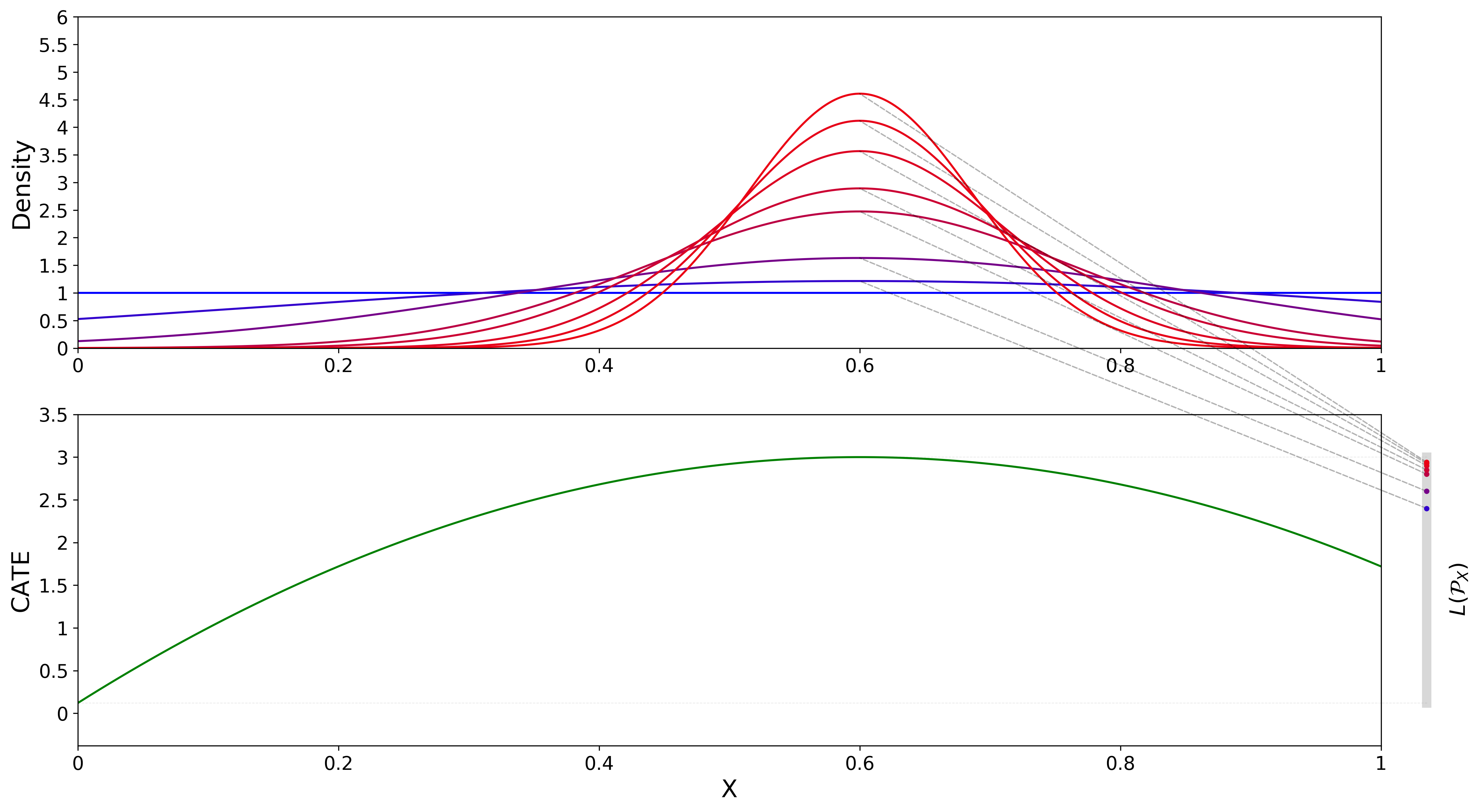
Figure 2: Local to boundary conditions. The lower panel displays the conditional average treatment effect, $\tau(x)$ for a univariate variable $X$. The experimental distribution is in blue: the uniform distribution. The gray segment on the left labelled $L(\mathcal{P}_{X})$ is the image of the collection of probability distributions supported on $\mathcal{X}$ under the map $L:F_{X}\mapsto\int_{\mathcal{X}}\tau(x)dF_{X}(x)$. For every point in the interior, Lemma 7 holds and, for each $\tilde{\tau}_{m}$, there is an associated least favorable distribution $F_{X,m}^{*}$ displayed in the upper panel. As the sequence of $\tilde{\tau}_{m}$ approaches the boundary of $L(\mathcal{P}_{X})$, the distributions concentrate around $x=\arg\max\tau(x)=0.6$.

For each $\tilde{\tau}_{m}$ within the range of variation of $\tau(X)$, the policy-maker’s problem has a solution, $F_{X,m}^{*}$ given by Lemma 7. This is because there is a sub-population with covariates $x$ such that $\tau(x)\geq\tilde{\tau}_{m}$. The least favorable distribution will increase the weight on this sub-population. If $\tilde{\tau}$ is on the boundary, for example $\tilde{\tau}=3$ in Figure 2, the only sub-population that has $\tau(x)\geq\tilde{\tau}_{b}$ is $x=0.6$, concentrated on a singleton. But distributions that put unit mass on singletons are not feasible in the policy-maker’s problem. For $\tilde{\tau}=\tilde{\tau}_{b}$, the feasible set is empty so there is no solution. If one looks at the sequence of least favorable distributions, $F_{X,m}^{*}$, associated to the sequence $\tilde{\tau}_{m}\rightarrow\tilde{\tau}_{b}$, is there a limiting distribution to which the sequence $F_{X,m}^{*}$ converges in some sense?

Under some additional assumptions, one can show a type of concentration result for the sequence of solutions obtained by applying the closed-from solution formula in Lemma 7. If $\tau(x)$ is a single peaked function, that is, it achieves its maximum (or minimum) at a single point, we obtain convergence in distribution of the sequence $F_{X,m}^{*}$ to the Dirac distribution at the single peak, $\delta_{x_{b}}$.

Proposition 10 (Local to boundary $\tilde{\tau}$).

Let Assumptions 1-3 hold and let $\tilde{\tau}_{m}\rightarrow\tilde{\tau}_{b}\in\partial L(\mathcal{P}_{X})$. Assume that the pre-image $\tau^{-1}(\tilde{\tau}_{b})=\mathcal{X}_{b}=\{x_{b}\}\in\mathcal{X}^{\mathsf{o}}$ is a singleton. Further, let $X$ be compactly supported, with density $f(x)<M$ on $\mathcal{X}$. Then the sequence of least favorable distributions for the policy-maker’s problem with parameter $\tilde{\tau}_{m}$, denoted $F_{X,m}^{*}$, converges weakly to $\delta_{x_{b}}$, the Dirac delta distribution with point mass at $x_{b}$, that is:

$$\lim_{m\to\infty}\int_{\mathcal{X}}g(x)dF_{X,m}^{*}(x)\rightarrow\int_{\mathcal{X}}g(x)\delta_{x_{b}}:=g(x_{b})$$

for $g\in C_{b}(\mathcal{X})$, the space of all continuous, bounded functions on $\mathcal{X}$.

• See Appendix E. ∎

The point-mass distribution $\delta_{x_{b}}$ is not a solution to the policy-maker’s problem with parameter $\tilde{\tau}_{b}$ because the feasible set never includes point mass distributions unless $\mathcal{X}$ is discrete. In this sense, Proposition 10 delivers the limit of the sequence of solutions in the sense of weak convergence. This is a weaker that the notion of convergence induced by $D_{KL}$. In particular when $dF_{X}\ll\lambda_{Leb}$ (the Lebesgue measure on $\mathbb{R}^{k}$), $D_{KL}(dF^{*}_{X,m}||\delta_{x_{b}})=+\infty$ so the sequence of solutions $F^{*}_{X,m}$ does not converge to $\delta_{x_{b}}$ in $D_{KL}$.

2.5 Benchmarking robustness using census covariates

This section develops an heuristic to interpret the robustness metric proposed in Definition 16. Several papers have proposed benchmarking the sensitivity to unobservable variables, which is often not computable, using observable variables. For example, Cinelli and Hazlett [2020] and Oster [2019] who use the explanatory power of observed covariates to benchmark for the explanatory power of unobserved covariates. This section suggests a similar approach for the robustness problem. In the context of this paper I would like to quantify whether a given value for the robustness parameter, $\delta^{*}$ is high or low. To this end I propose to leverage the subset of covariates in $X_{c}$, which are available in both the quasi-experimental environment and in the extrapolation environment to benchmark the robustness measure. At the population level it amounts to:

• computing the robustness metric $\delta^{*}$ through Equation (10)

• use the census information to compute $D_{KL}(P^{\prime}_{X_{c}}||P_{X_{c}})$, the KL divergence between the distributions of the $X_{c}$ covariates in the quasi-experimental population and the new population

• compare the two measures

If the variables in $X_{c}$ collectively differ across the two environments by the same amount as $X_{e}$, observing $\delta^{*}>D_{KL}(P^{\prime}_{X_{c}}||P_{X_{c}})$ suggests that the quasi-experimental claim can be extrapolated to the new environment. In words, it says that the distance, measured by the KL divergence between the observable census variables in the two environments would not be large enough to invalidate the claim drawn from the quasi-experimental evidence. In principle, one could develop a formal test that uses both $\delta^{*}$ and $D_{KL}(P^{\prime}_{X_{c}}||P_{X_{c}})$ (under the assumption that the true distance in $X_{e}$ is no larger than the true distance in $X_{c}$) to provide a pessimistic policy-maker with a clear rule on when to expand the policy given the census data. For now, transforming the heuristic exercise above in a full fledged two-sample test is beyond the scope of this paper and I leave it to future research.

3 Estimation and Asymptotic Results

In this section I introduce a semi-parametric estimator for my robustness metric $\delta^{*}$, according to Definition 3 ii) and I characterize its asymptotic properties. I show that the robustness metric can be estimated using a GMM criterion function which only depends on the quasi-experimental distribution and on the CATE $\tau(x)$, both of which are identified in the quasi experiment. The theory is based on constructing the nonparametric influence function correction for the de-biased GMM procedure in Chernozhukov et al. [2020] to account for flexible nonparametric estimation of $\tau(x)$. The proofs are in the Appendix E.

3.1 An empirical estimate of the robustness metric $\delta^{*}$

The closed form solution in Lemma 7 suggests a natural estimator based on empirical averages. In particular, one would like to replace Equation (10) with its sample analog using the Generalized Method of Moments (GMM) framework. Consider the quantities:

$$\nu_{0}:=\int_{\mathcal{X}}\exp(-\lambda_{0}(\tau(x)-\tilde{\tau}))dF_{X}(x)$$

where $\lambda_{0}$ is defined implicitly as the unique solution to:

$$\int_{\mathcal{X}}\exp(-\lambda_{0}(\tau(x)-\tilde{\tau}))(\tau(x)-\tilde{\tau})dF_{X}(x)=0$$

The pair of parameters that solves the population moment condition is denoted by $\theta_{0}=(\nu_{0},\lambda_{0})^{T}$. Ultimately, the robustness measure $\delta^{*}=-\log(\nu_{0})$ is the parameter of interest. The asymptotic theory for $\delta^{*}$ follows directly from establishing the asymptotic theory for $\hat{\theta}=(\hat{\nu},\hat{\lambda})^{T}$ hence, I will focus on these parameters in this section. The parameter space $\Theta\subseteq\mathbb{R}^{2}$ satisfies some constraints. First, observe that if the policy-maker’s claim ($ATE\geq\tilde{\tau}$) holds with a strict inequality for the quasi-experimental distribution, then the true $\delta^{*}>0$. This implies a restriction on $\nu_{0}<1$. Moreover, $\nu_{0}>0$ because by the properties of the exponential, the quantity $\exp(-\lambda(\tau(x)-\tilde{\tau})>0$ for all $x\in\mathcal{X}$. Hence, the restriction on $\nu$ is $0\leq\nu_{0}\leq 1$.

Let $W=(X,D,Y)$ be the data. Then, as in Newey and McFadden [1994] we can write the moment condition jointly for $\nu_{0}$ and $\lambda_{0}$ as:

$$\mathbb{E}[g(W,\theta,\tau)]=\mathbb{E}\begin{bmatrix}\exp(-\lambda_{0}(\tau_{0}(X)-\tilde{\tau}))-\nu_{0}\\ \exp(-\lambda_{0}(\tau_{0}(X)-\tilde{\tau}))(\tau_{0}(X)-\tilde{\tau})\end{bmatrix}=\begin{bmatrix}0\\ 0\end{bmatrix}$$ (13)

where $\tau_{0}(X)$ denotes the true value of CATE. Assumptions 1–4 guarantee that the parameters of interest $(\lambda_{0},\nu_{0})$ are (globally) identified by Equation (13). Because the true value for $\tau_{0}(X)$ is an unknown but estimable population quantity, I consider a feasible version of Equation (13) that uses an estimate $\hat{\tau}(X)$ in place of $\tau_{0}(X)$. One could define the vector $\hat{\theta}=(\hat{\lambda},\hat{\nu})^{T}$ is defined as the approximate solution to the empirical moment:

$$\mathbb{E}_{n}[g(W,\theta,\hat{\tau})] =\begin{bmatrix}\frac{1}{n}\sum_{i=1}^{n}\exp(-\hat{\lambda}(\hat{\tau}(X_{i})-\tilde{\tau}))-\hat{\nu}\\ \frac{1}{n}\sum_{i=1}^{n}\exp(-\hat{\lambda}(\hat{\tau}(X_{i})-\tilde{\tau}))(\hat{\tau}(X_{i})-\tilde{\tau})\end{bmatrix}=\begin{bmatrix}0\\ 0\end{bmatrix}$$ (14)

where $\hat{\tau}(X)$ is a plug-in estimate of the conditional average treatment effect. While Assumption 1 guarantees nonparametric identification of $\tau_{0}(X)$, there are many ways that one could estimate it, both parametrically and nonparametrically. For example Athey et al. [2016] uses random forest, Hsu et al. [2020] uses a doubly robust score function.

One caveat of the estimator based on Equation (14) is that the identifying moment conditions provided in Equation (13) are not Neyman orthogonal with respect to the first-step estimator $\hat{\tau}(X)$. As a result, the first-step estimation of $\hat{\tau}(X)$ can, in general, have a first-order effect on the estimator for $\theta_{0}=(\nu_{0},\lambda_{0})^{T}$, and consequently on the estimator for $\delta^{*}$, and possibly lead to incorrect inferences on the robustness metric, a general problem discussed in Chernozhukov et al. [2018]. Deriving primitive conditions on this form of the moment condition requires ad-hoc conditions on the first-step nonparametric estimator that can be hard or inconvenient to check in practice. As an alternative, I use the debiased-GMM approach in Chernozhukov et al. [2020] that allows to choose flexible estimators for $\tau_{0}(X)$ while automatically correcting for the first-order bias.

3.2 Nonparametric influence function correction and de-biased GMM estimator

In this section, I derive the nonparametric correction for the GMM estimator of $\theta$ based on Equation (14). I map the causal quantities like $\tau(X)$ to the statistical functionals that identify them and then explicitely construct the nonparametric influence function for these functionals. Because these functionals are always implicitly regarded as mapping the distribution function of the data, $F$, to some space, it is natural to index the functional with a subscript $F$. For example the $\tau(X)=\tau_{F}(X)$ because depends of the distribution of the data $F$. The true distribution of the data will be denoted as $F_{0}$ and it is understood that $\tau_{0}(X)=\tau_{F_{0}}(X)$. Recall that $\tau_{F_{0}}(X)$ is a causal parameter which needs to be identified through the distribution of the data. By Assumption 1, $\tau_{F_{0}}(X)$ can be nonparametrically identified as the difference between the conditional means: $\tau_{F_{0}}(X)=\gamma_{1,F_{0}}(X)-\gamma_{0,F_{0}}(X)$ where $\gamma_{1,F}(X):=\mathbb{E}_{F}[Y|X,D=1]$ and $\gamma_{0,F}(X):=\mathbb{E}_{F}[Y|X,D=0]$. The left hand side features a causal quantity while the right hand side features two statistical quantities. The first step then has two functions that need to be estimated. For convenience, I gather them into a single vector-valued statistical functional $\gamma_{F}=(\gamma_{0,F},\gamma_{1,F})^{T}$. When considering the de-biasing term to correct for the first-step estimation of $\tau_{F_{0}}(X)$, we actually need to consider the first-step correction with respect to the full vector $\gamma_{F}$.

Now consider a parametric sub-model for the distribution function, consisting of $F_{r}:=(1-r)\cdot F_{0}+rH$ where $F_{0}$ is the true baseline distribution function of the data and $H$ is an arbitrary distribution function which satisfies Assumption 1. For any $r\in[0,1],F_{r}$ is a mixture distribution and hence, it is also a valid distribution function. Moreover, if both $F_{0}$ and $H$ satisfy Assumption 1 then $F_{r}$ does as well. In order to de-bias the moment conditions in $\mathbb{E}[g(W,\theta,\tau_{F})]$ with the approach of Chernozhukov et al. [2020] one needs to compute the nonparametric influence function with respect to $\tau_{F}$. The nonparametric influence function maps infinitesimal perturbations of $F$ in the direction of $H$ in a neighborhood of $F_{0}$, to perturbations in $\mathbb{R}^{2}$ (because there are 2 moment conditions). It does so linearly in $H$. In particular, the nonparametric influence function of $\mathbb{E}[g(W,\theta,\tau_{F})]$ with respect to $F$, labelled $\phi(\cdot)$ is implicitly defined by the equation below:

$$\frac{d\mathbb{E}[g(W,\theta,\gamma_{F_{r}})]}{dr}\Bigg{|}_{r=0}=\int\phi(w,\gamma_{F_{0}},\theta,\alpha)dH(w)$$ (15)

Note that, other than the original arguments of $g(\cdot)$, which feature the vector of conditional means $\gamma_{F_{0}}$, $\phi(\cdot)$ is allowed to depend on additional nonparametric components, gathered in $\alpha(\cdot)$. In the next result I derive the nonparametric influence function explicitly.

Proposition 11.

The de-biased GMM nonparametric influence function based on moment function $g(\cdot)$ is:

$$\phi(w,\theta,\gamma_{0},\alpha_{0}) =\begin{bmatrix}\exp\left(-\lambda\cdot(\gamma_{1,F_{0}}(x)-\gamma_{0,F_{0}}(x)-\tilde{\tau})\right)\cdot(-\lambda)\\ \exp\left(-\lambda\cdot(\gamma_{1,F_{0}}(x)-\gamma_{0,F_{0}}(x)-\tilde{\tau})\right)\cdot(1-\lambda\cdot(\gamma_{1,F_{0}}(x)-\gamma_{0,F_{0}}(x)-\tilde{\tau}))\end{bmatrix}$$

$$\times\left(\frac{d(y-\gamma_{1,F_{0}}(x))}{\pi_{F_{0}}(x)}-\frac{(1-d)(y-\gamma_{0,F_{0}}(x))}{1-\pi_{F_{0}}(x)}\right)$$

which could be written in the form:

$$\phi(w,\theta,\gamma_{0},\alpha_{0}) =\begin{bmatrix}\exp\left(-\lambda\cdot(\gamma_{1,F_{0}}(x)-\gamma_{0,F_{0}}(x)-\tilde{\tau})\right)\cdot(-\lambda)\\ \exp\left(-\lambda\cdot(\gamma_{1,F_{0}}(x)-\gamma_{0,F_{0}}(x)-\tilde{\tau})\right)\cdot(1-\lambda\cdot(\gamma_{1,F_{0}}(x)-\gamma_{0,F_{0}}(x)-\tilde{\tau}))\end{bmatrix}$$

$$\times\left(\begin{bmatrix}\alpha_{1,F_{0}}(x)\\ \alpha_{0,F_{0}}(x)\end{bmatrix}^{T}\begin{bmatrix}d(y-\gamma_{1,F_{0}}(x))\\ (1-d)(y-\gamma_{0,F_{0}}(x))\end{bmatrix}\right)$$

with $\alpha_{F_{0}}(x):=\begin{bmatrix}\alpha_{1,F_{0}}(x)\\ \alpha_{0,F_{0}}(x)\end{bmatrix}=\begin{bmatrix}\frac{1}{\pi_{F_{0}}(x)}\\ \frac{1}{1-\pi_{F_{0}}(x)}\end{bmatrix}$.

There are two main multiplicative terms in $\phi(\cdot)$. The first term is the derivative of the moment conditions with respect to the first-step estimator. The second one is the variation of individual treatment effects about their conditional mean, appropriately weighted by the propensity score. One can immediately check that, by the law of iterated expectations, $\mathbb{E}_{F}[\phi(W,\theta,\gamma_{0},\alpha_{0})]=0$ for any $\theta$. Hence we can form the de-biased GMM moment functions by taking:

$$\psi(w,\gamma,\theta,\alpha)=g(w,\theta,\gamma)+\phi(w,\theta,\gamma,\alpha)$$ (16)

Notice that $\mathbb{E}_{F_{0}}[\psi(W,\theta,\gamma_{0},\alpha_{0})]=0$ so an estimator for $\theta$ that uses the de-biased moment function $\psi(\cdot)$ instead of $g(\cdot)$ will preserve identification. Standard conditions can be given to guarantee $\mathbb{V}[\psi(W,\theta,\gamma_{0},\alpha_{0})]<\infty$ so that $\psi(W_{i},\theta,\gamma_{0},\alpha_{0})$ is a valid influence function. As emphasized in Chernozhukov et al. [2020] the de-biased GMM form of $\psi(\cdot)$ corrects for the first order bias induced by replacing $\gamma_{1,F_{0}}-\gamma_{0,F_{0}}$, the statistical counterpart of the true $\tau_{F_{0}}$, with a flexibly estimated $\hat{\gamma}_{1}-\hat{\gamma}_{0}$. In particular, for $\sqrt{n}$-consistency of $\theta$, the estimators for $\hat{\gamma}_{1}$ and $\hat{\gamma}_{0}$ only need to satisfy mild conditions on the $L^{2}$-rate of convergence in Assumption 5 below. This allows to characterize simple inference for the robustness measure $\hat{\delta}^{*}$ while allowing for flexible nonparametric estimation of $\gamma_{1,F_{0}}$ and $\gamma_{0,F_{0}}$ using a large collection of machine learning-based estimators which include, among others, random forest, boosting, and neural nets. In practice, machine learning methods can help when the covariate space is high-dimensional but the true $\tau_{0}(X)$ has a sparse representation.

The key property to guarantee de-biasing is given by the Neyman orthogonality of the new moment conditions with respect to the first-step estimator, established in the result below.

Proposition 12.

Equation (16) satisfies Neyman orthogonality.

• See Appendix E. ∎

Consider now the empirical version of the de-biased GMM equations:

$$\hat{\psi}(\theta,\hat{\gamma},\hat{\alpha})=\frac{1}{K}\sum_{k=1}^{K}\frac{1}{|I_{k}|}\sum_{i\in I_{k}}\left(g(W_{i},\theta,\hat{\gamma}_{-k})+\phi(W_{i},\tilde{\theta},\hat{\gamma}_{-k},\hat{\alpha}_{-k})\right)$$

The de-biased GMM estimator takes advantage of a cross-fitting procedure where the sample is split into $K$ many folds. For each fold $k=1,\cdots,K$, the nonparametric components in $\psi(\cdot)$, that is, the $\gamma(\cdot)$ and $\alpha(\cdot)$ functions, are estimated on the observations in the remaining $(K-1)$ folds which explains the indexing $-k$ in the subscripts of $\gamma(\cdot)$ and $\alpha(\cdot)$. Sample splitting reduces own-observation bias and, together with the Neymann orthogonality property established above, avoids complicated Donsker-type conditions that would potentially not be satisfied for some first-step estimators of $\hat{\gamma}$ and $\hat{\alpha}$, as discussed in Chernozhukov et al. [2020]. Finally note that $\tilde{\theta}$ is a consistent estimator for $\theta$ needed to evaluate $\phi$. For example one could use the $\theta$ from the plug-in GMM which is consistent but may not be $\sqrt{n}$-consistent in general. The de-biased GMM estimator is given by:

$$\hat{\theta}=\arg\min_{\theta\in\Theta}\hat{\psi}(\theta,\hat{\gamma},\hat{\alpha})$$ (17)

To establish $\sqrt{n}$-convergence of the GMM estimators for $\theta$, some quality conditions on the $L_{2}$ rates of convergence of the first-step estimators for $\gamma$ and $\alpha$ are required.

Assumption 5.

For any $k$, $\lVert\hat{\gamma}_{-k}-\gamma_{0}\rVert_{L}^{2}=o_{P}(N^{-\frac{1}{4}});\lVert\hat{\alpha}_{-k}-\alpha_{0}\rVert_{L}^{2}=o_{P}(1)$.

In Appendix E, I use Assumptions 1 – 5 to prove the influence function representation for $\hat{\theta}$ to which a standard central limit theorem applies to establish the asymptotic normality of the de-biased GMM estimator for $\theta=(\nu,\lambda)^{T}$. This, in turn, allows to conduct inference on the parameter of interest, $\delta^{*}$ through a straightforward application of the delta method.

Theorem 13 (Asymptotic normality of $\theta$).

Let Assumptions 1–5. For $\hat{\theta}$ defined in Equation (17):

$$\sqrt{n}(\hat{\theta}-\theta_{0})\overset{d}{\rightarrow}\mathcal{N}(0,S)$$

$$S :=(G)^{-1}\Omega(G^{\prime})^{-1}$$

$$G :=\mathbb{E}[D_{\theta}\psi(w,\theta,\gamma_{0},\alpha_{0})]$$

$$\Omega :=\mathbb{E}[\psi(w,\theta_{0},\gamma_{0},\alpha_{0})\psi(w,\theta_{0},\gamma_{0},\alpha_{0})^{T}]$$

and $D_{\theta}\psi(\cdot)$ is the Jacobian of the augmented moment condition with respect to the parameters in $\theta$.

• See Appendix E. ∎

The parameter of interest follows from a straightforward application of the parametric delta method.

Corollary 14 (Asymptotic normality of $\delta^{*}$).

Let $\hat{\delta}^{*}=-\log(\hat{\nu})$. Then

$$\sqrt{N}(\hat{\delta}^{*}-\delta^{*})\overset{d}{\rightarrow}\mathcal{N}\left(0,\frac{S_{11}}{\nu_{0}^{2}}\right)$$

where $S_{11}$ is the (1,1) entry of the variance covariance matrix S in Theorem 13.

With the results of Theorem 13 one can obtain a point estimate $\delta^{*}$, together with a confidence interval for a pre-specified coverage level. Because of the nature of the estimand, the researcher or the policy-maker, are likely to care especially about the lower bound for $\delta^{*}$. This is because overestimating the $\delta^{*}$ implies that there is a distribution of the covariates within the estimated $\hat{\delta^{*}}$ that invalidates the policy-maker’s claim. This defies the entire purpose of the robustness exercise. On the other hand, underestimating $\delta^{*}$ may result in unduly conservative characterization of the set of distributions for which the claim is valid, but it does not defy the purpose of the robustness exercise. A similar, asymmetric approach is followed by Masten and Poirier [2020] who report a lower confidence region for their breakdown frontier rather than a confidence band.

3.3 Reporting features of the least favorable distribution

Lemma 7 gives an explicit formula for the least favorable distribution $F_{X}^{*}$, the minimizer of Equation (4), and shows that it depends on $\lambda_{0}$ and $\tau(X)$. The rate of convergence of as estimator of $F^{*}_{X}$ can, in general, be nonparametric. This is because, under some conditions, it inherits the nonparametric rate of $\hat{\tau}(X)$. If $\mathcal{X}\subseteq\mathbb{R}^{d}$ is even moderately high dimensional, it may be very inconvenient to look at features of the estimated $F^{*}_{X}$. Rather, the researcher could report particular moments of $F_{X}^{*}$ that are of interest. This exercise is analogous to reporting moments of the covariate distribution and compare them across treatment status to gauge at covariate balance, like in Rosenbaum and Rubin [1984]. The researchers may want to report moments of $F_{X}^{*}$, in addition to the robustness metric $\delta^{*}$. For example they may want to report a vector of covariate means under the least favorable distribution $F^{*}_{X}$ and compare it with the quasi-experimental distribution. In such a case, we would like to construct an estimator for the moments of interest and establish the asymptotic theory of these estimators. I give a convenient extension of Theorem 13, to include an arbitrary, finite dimensional collection $\zeta\in\mathbb{R}^{s}$ of moments of interest, along with the original $\theta$ parameters.

Theorem 15 (De-biased estimator of least favorable moments).

Let $u:\mathbb{R}^{d}\rightarrow\mathbb{R}^{s}$, with $u\in(L^{\infty}(\mathcal{X},\mu))^{s}$ for $\mu$ some dominating measure of $P_{X}$. Let $\zeta_{0}=\mathbb{E}_{F^{*}_{X}}[u(X)]\in\mathbb{R}^{s}$. Define the following estimating equation for the parameters $(\hat{\theta},\hat{\zeta})$, that is, the original parameters of interest, augmented by $\zeta$, the additional moments of the least favorable distribution:

$$\hat{\psi}^{u}(\theta,\zeta,\hat{\gamma},\hat{\alpha}):=\frac{1}{K}\sum_{k=1}^{K}\frac{1}{|I_{k}|}\sum_{i\in I_{k}}\begin{bmatrix}g(W_{i},\theta,\hat{\gamma}_{-k})+\phi(W_{i},\theta,\hat{\gamma}_{-k},\hat{\alpha}_{-k})\\ g^{u}(W_{i},\theta,\zeta,\gamma_{-k})+\phi^{u}(W_{i},\theta,\zeta,\hat{\gamma}_{-k},\hat{\alpha}_{-k})\end{bmatrix}$$

where $g(\cdot),\phi(\cdot),\gamma(\cdot)$ and $\alpha(\cdot)$ are the same as in Propositions 11 – 24 and $g^{u}(\cdot)$ and $\phi^{u}(\cdot)$, whose values are vectors in $\mathbb{R}^{s}$ are defined below.

$$g^{u}(W_{i},\theta,\zeta,\gamma) =u(X_{i})\exp(-\lambda(\tau(X_{i})-\tilde{\tau})-\nu\cdot\zeta$$

$$\phi^{u}(W_{i},\theta,\zeta,\gamma,\alpha) =u(X_{i})\exp\left(-\lambda(\tau(X_{i})-\tilde{\tau})\right)\cdot(-\lambda)$$

$$\times\left(\frac{D_{i}(Y_{i}-\gamma_{1}(X_{i}))}{\pi(X_{i})}-\frac{(1-D_{i})(Y_{i}-\gamma_{0}(X_{i}))}{1-\pi(X_{i})}\right)$$

$$(\hat{\theta},\hat{\zeta}):=\arg\min_{(\theta,\zeta)\in\mathbb{R}^{s+2}}\hat{\psi}^{u}(\theta,\zeta,\hat{\gamma},\hat{\alpha})^{T}\hat{\psi}^{u}(\theta,\zeta,\hat{\gamma},\hat{\alpha})+o_{P}(1)$$ (18)

Let Assumptions 1–5 hold. Then:

$$\frac{1}{\sqrt{n}}\sum_{k=1}^{K}\sum_{i\in I_{k}}\psi^{u}(W_{i},\theta,\zeta,\hat{\gamma}_{-k},\hat{\alpha}_{-k})=\frac{1}{\sqrt{n}}\sum_{i=1}^{n}\psi^{u}(W_{i},\theta,\zeta,\gamma_{0},\alpha_{0})+o_{P}(1)$$

Moreover

$$\sqrt{n}\left(\begin{bmatrix}\hat{\theta}-\theta_{0}\\ \hat{\zeta}-\zeta_{0}\end{bmatrix}\right)\overset{d}{\rightarrow}\mathcal{N}(0,S^{u})$$

$$S^{u} :=(G^{u})^{-1}\Omega^{u}(G^{u^{\prime}})^{-1}$$

$$G^{u} :=\mathbb{E}[D_{\theta,\zeta}\ \psi^{u}(W,\theta,\zeta,\gamma_{0},\alpha_{0})]$$

$$\Omega^{u} :=\mathbb{E}[\psi^{u}(w,\theta_{0},\gamma_{0},\alpha_{0})^{T}\psi^{u}(w,\theta_{0},\gamma_{0},\alpha_{0})]$$

where $D_{\theta,\zeta}$ denotes the Jacobian matrix with respect to the parameters $\theta$ and $\zeta$.

• The proof follows the same structure of Theorem 13 and is omitted. ∎

3.4 Simulation data

I conclude this section with a small Monte-Carlo exercise featuring three different data generating processes (DGPs) with increasing degrees of observable heterogeneity. To capture the idea of possibly high-dimensional experimental data, I consider a setting with $k=100$ covariates, all independent and each distributed uniformly on $[0,1]$ so that $\mathcal{X}$ = $[0,1]^{k}$. To reflect the fact that only a few out of all available experimental covariates are important to predict the treatment effect, I construct $\tau(x)$ to be sparse: $\tau(x)$ is a function of of only 1,3 and 10 out of 100 covariates in DGP1, DGP2 and DGP3 respectively. In each DGP, the potential outcomes also depend on an additive unobservable noisy error term. To show that it is the heterogeneity that drives the robustness, keeping the same baseline ATE for the three DGPs is fundamental. I choose the shape of $\tau(x)$ to induce the same ATE across the three DGPs, regardless of the heterogeneity of treatment effects, when evaluated with respect to the experimental distribution. I consider $M=1000$ replications for each DGP and a sample size of $N=10,000$. The first step $\tau(x)$ is estimated through K-fold cross-fitting, using either boosting or random forest to estimate $\gamma_{1}(x)$, $\gamma_{0}(x)$ and the propensity score $\pi_{X}(x)$. The number of trees and splitting criteria are tuned to the sample size through heuristic criteria. In practice one would use within-fold cross-validation to tune hyper-parameters. I estimate the implied $\hat{\delta}^{*}(\tilde{\tau})$, with $\tilde{\tau}=1.3$ and evaluate its bias, variance and MSE against the true value $\delta^{*}$. Fixing the ATE and the experimental distribution of the covariates guarantees that a change in the population value for $\delta^{*}$ is only capturing the change in heterogeneity. I report the estimates of $\delta^{*}$ using both the plug-in GMM and de-biased GMM approach below. Note that, because of K-fold cross fitting, the own-observation bias in the plug-in GMM is attenuated. Still, the de-biased, GMM shows very good bias improvements over the plug-in approach.

Data $\delta^{*}(\tilde{\tau})$ Method $\gamma(\cdot)$, $\alpha(\cdot)$ est MSE Bias² Variance DGP1 0.4485 plug-in Random Forest $3.7568\cdot 10^{-4}$ $0.1235\cdot 10^{-4}$ $3.6334\cdot 10^{-4}$ Boosting $1.6311\cdot 10^{-3}$ $1.2056\cdot 10^{-3}$ $0.4255\cdot 10^{-3}$ de-biased Random Forest $3.7148\cdot 10^{-4}$ $0.1030\cdot 10^{-4}$ $3.6117\cdot 10^{-4}$ Boosting $1.5278\cdot 10^{-3}$ $1.1038\cdot 10^{-3}$ $0.4240\cdot 10^{-3}$ DGP2 0.1344 plug-in Random Forest $5.0716\cdot 10^{-3}$ $4.9474\cdot 10^{-3}$ $0.1242\cdot 10^{-3}$ Boosting $1.1218\cdot 10^{-3}$ $1.0622\cdot 10^{-3}$ $0.0597\cdot 10^{-3}$ de-biased Random Forest $3.6640\cdot 10^{-3}$ $3.5616\cdot 10^{-3}$ $0.1024\cdot 10^{-3}$ Boosting $0.7309\cdot 10^{-3}$ $0.6749\cdot 10^{-3}$ $0.0560\cdot 10^{-3}$ DGP3 0.1328 plug-in Random Forest $5.2825\cdot 10^{-3}$ $5.1558\cdot 10^{-3}$ $0.1267\cdot 10^{-3}$ Boosting $1.4637\cdot 10^{-3}$ $1.3991\cdot 10^{-3}$ $0.0646\cdot 10^{-3}$ de-biased Random Forest $3.8369\cdot 10^{-3}$ $3.7326\cdot 10^{-3}$ $0.1043\cdot 10^{-3}$ Boosting $0.9312\cdot 10^{-3}$ $0.8716\cdot 10^{-3}$ $0.0596\cdot 10^{-3}$

Table 1: Monte Carlo Simulation reports the DGP, the population value for the robustness metrics, ML estimator used for the nonparametric components and MSE, Bias and Variance. Sample size $n=10,000$, number of simulations $M=1000$.

Table 1 report the results. First, observe the reduction in the population value of $\delta^{*}(\tilde{\tau})$ as heterogeneity increases in the DGP. This is entirely driven by an increase in the heterogeneity of $\tau(x)$ since the ATE is the same across the three DGPs. This means that a smaller shift in the covariates is required to invalidate the policy-maker claim ($ATE\geq 1.3$). As a result, the robustness metric decreases. Moving from DGP1 to DGP2 and DGP3 the population value of the robustness metric drops from 0.4485 to 0.1344 to 0.1328. The decrease is most accentuated between DGP1 and DGP2 because of the functional form of $\tau(x)$.

In DGP1 we can see that the heuristic choice for the hyper-parameters in boosting likely results in under-fitting the data, leading to a bias an order of magnitude higher than the variance. For DGP1, the de-biasing procedure results in approximately 20% squared bias reduction which drives the reduction of approximately the same percentage in the Mean Squared Error. Variances are comparable between plug-in and de-biased GMM. The random forest procedure is better overall for MSE criterion. In DGP2, the bias dominate the variance component, suggesting both random forest and boosting are under-fitting. This is likely do to the absence of a within-fold cross-validation step. In this case,the de-biased GMM reduces the squared bias by about 40% for both random forest and boosting methods. The variances are again very similar across plug-in and de-biased and boosting has about half of the variance of random forest. DGP3’s heterogeneity increases slightly, reducing the associated $\delta^{*}(\tilde{\tau})$. Like in DGP2, the bias dominates the variance component regardless of the first-step estimation method. Similarly, the de-biased GMM approach results in substantial bias reduction in comparison to the plug-in GMM approach.

4 Empirical Application: How robust are the effect of the Oregon Medicaid expansion?

In this section, I apply my approach to study the robustness of health insurance policy with respect to shifts in the distribution of covariates. The key reference is Finkelstein et al. [2012], which uses experimental data to study the effect of the Oregon Medicaid expansion lottery on health-care consumption and financial outcomes. The positive results of the study are of great interest for any policy-maker who is potentially interested in implementing a similar intervention in their state. Because the populations of recipients are likely to differ across states, I propose to complement the experimental result in Finkelstein et al. [2012] with an estimate of my robustness metric $\delta^{*}$ to quantify the smallest shift in important experimental covariates needed to eliminate the positive effects of the insurance lottery.

4.1 Institutional context and heterogeneity

Between March and September 2008, the state of Oregon conducted a series of lottery draws that would award the selected individuals the option to enroll in the Oregon Health Plan (OHP) Standard. OHP Standard is a Medicaid expansion program available for Oregon adult residents that are between 19 and 64 years of age and have limited income and assets. Finkelstein et al. [2012] studies the effect of the insurance coverage on a set of metrics that include health-care utilization (number of prescription, inpatient, outpatient and ER visits), recommended preventive care (cholesterol and diabetes blood test, mammogram and pap-smear test) and measures of financial strain (outstanding medical debt, denied care, borrow/default). The study uses both administrative and survey data but only the survey data is publicly accessible through Finkelstein [2013]. The Online appendix of Finkelstein et al. [2012] discusses a variety of robustness concerns that center on external validity. For example they note that scaling up the experiment can induce a supply side change in providers’ behavior. Additionally, they acknowledge substantial demographic differences between the study population in Oregon versus the potential recipients in other states. These differences include, for example, a smaller African American and a larger white sub-population in Oregon versus other states. From the survey data it appears that the Oregon lottery participants are older and their health metrics under-performs the national average. If these covariates are important in determining the treatment effects of the health insurance, the results of Oregon experiment may not be robust to a change in the distribution of covariates. This robustness is especially important to quantify if the experimental results are to be extrapolated for policy adoption in other states. I stress the fact that, in this context, the re-weighting procedure in Hartman [2020] or Hsu et al. [2020] is not applicable because it lacks the survey-specific health data that are likely to be most predictive of treatment effect heterogeneity. Absent full covariate data form other states, I proposed to study the robustness of the policy by augmenting each of the treatment effect estimators in Finkelstein et al. [2012] with my robustness metric, which can be computed by exploiting the heterogeneity in the publicly available survey data [Finkelstein, 2013].

4.2 Robustness in the Oregon Medicaid Experiment

For the robustness exercise I focus on the Intention to Treat Effect (ITT) of the Oregon Medicaid Experiment lottery. As noted in Finkelstein et al. [2012], not all recipients who were awarded the option to enroll in the insurance program actually enrolled. For this reason Finkelstein et al. [2012] estimates both an ITT and a LATE estimate. One could argue that the ITT is the key parameter for a policy-maker interested in offering the same intervention. To map my framework to the application, recall that the ITT effect can be considered as an ATE where the treatment $D$ is simply the “the option to enroll in the health insurance” so the robustness approach discussed in the paper carries over to the ITT with only notational changes. I consider hypotheses of the form $ITT_{j}\geq\tilde{\tau}$ or $ITT_{j}\leq\tilde{\tau}$ (depending on the outcome measure of interest) where $j$ indexes a health-care utilization or a financial strain outcome, following the notation convention in Finkelstein et al. [2012]. As noted in Finkelstein et al. [2012] all health-care utilization outcomes are defined consistently so that a positive sign for ITT means an increase in utilization. Similarly, all financial strain outcomes are defined so that a negative sign for the ITT means a decrease in financial strain. I focus on 2 value of interest for $\tilde{\tau}$ for each of the outcome measures. One of the values is $\tilde{\tau}=0$ which reflects the claim that the ITT is non-negative (for health-care utilization outcomes), or non-positive (for financial strain outcomes). The second value is $\tilde{\tau}=t_{j}=z_{\alpha}\sigma_{j}$ where $\sigma_{j}$ is the standard deviation of the ITT for outcome $j$. $t_{j}$ is the critical value for the $t$-statistic of a one sided test with null hypothesis $ITT\leq 0$ for some pre-specified $\alpha$. As a result $\delta(t_{j})$ proxies for the magnitude of a change in the covariate distribution that would make the ITT statistically not distinguishable from a non-positive or non-negative outcome (respectively). Because $\sigma_{j}$ is in general not available, in the empirical procedure I use $\hat{\sigma}_{j}$ in place of $\sigma_{j}$. The researcher interested in different hypothesis may adapt the procedure easily by specifying a $\tilde{\tau}$ with a value different from the two discussed above.

For the application I group the outcome measure in three groups: measure of health-care utilization, measures of compliance with recommended preventive care and measures of financial strain. I replicate the estimates of the intention to treat effect (ITT) for outcome variables in each of the three groups in Finkelstein et al. [2012] from a reduced form regression of the outcome variable on the lottery indicator and controls. The regression includes survey waves indicators, household size indicators and interaction terms between the two as controls. Because the regression is fully saturated, the estimates for the ITT are nonparametric. In my robustness exercise I focus on covariates that appear critical for external validity and are likely to differ across states. Among others, Finkelstein et al. [2012] identifies gender, age, race, credit access, education and proxies for health status. To capture the potential heterogeneity, I estimate a Conditional Intention to Treat effect (CITT) with the set of covariates listed above. Finally I use the estimated CITT to compute the measure of robustness $\delta^{*}$ for each of the outcome variables in the three categories and report it, together with the original ITT estimate, for both values of $\tilde{\tau}$ discussed above. All outcomes are measured on the survey data [Finkelstein, 2013].

In Table 2, column 2, 3 and 4 contain respectively the experimental ITT for each outcome variable, the estimates for $\delta^{*}(0)$ and the estimates for $\delta^{*}(t_{j})$. Here $t_{j}=\pm 1.645\cdot\sigma_{j}$ depending on whether the experimental ITT is positive or negative. As an example, consider a measure of financial strain, like whether a patient had to borrow or skip a payment because of medical debt. The intention to treat effect is equal to -0.0515 with standard error 0.0060. $\delta^{*}(0)=0.367$ represents the smallest distributional shift of the covariates that can induce an ITT equal to 0. The $\delta^{*}(t_{j})=0.265$ represents the smallest distributional shift in the covariates that can result in an $ITT=-1.645\cdot 0.0060=-0.0118$ which leads to not rejecting the hypothesis $H_{0}:ITT\geq 0$. For any distributional shift that is smaller than $\delta^{*}(t_{j})$ the statistical claim $H_{0}:ITT\geq 0$ would be rejected.

Outcome	Experimental ATE	$\delta^{*}(0)$	$\delta^{*}(t_{j})$
health-care Utilization
Prescriptions	$\underset{(0.044)}{0.1296}$	$\underset{(0.007)}{0.380}$	$\underset{(0.002)}{0.068}$
Out-patient visits	$\underset{(0.039)}{0.2986}$	$\underset{(0.022)}{1.552}$	$\underset{(0.014)}{0.965}$
ER visits	$\underset{(0.013)}{0.0064}$	$\underset{(0.001)}{0.009}$	$\underset{n/a}{0}$
In-patient visits	$\underset{(0.005)}{0.0081}$	$\underset{(0.003)}{0.119}$	$\underset{n/a}{0}$
Financial Strain
Out of pocket expenses	$\underset{(0.0069)}{-0.0622}$	$\underset{(0.030)}{0.462}$	$\underset{(0.023)}{0.346}$
Outstanding expenses	$\underset{(0.0070)}{-0.0529}$	$\underset{(0.0231)}{0.290}$	$\underset{(0.016)}{0.204}$
Borrow/Skip payments	$\underset{(0.0060)}{-0.0515}$	$\underset{(0.019)}{0.367}$	$\underset{(0.014)}{0.265}$
Refused care	$\underset{(0.0040)}{-0.011}$	$\underset{(0.006)}{0.063}$	$\underset{(0.002)}{0.013}$

Table 2: $\delta^{*}$ robustness metric for the health-care utilization and financial strain outcomes in Finkelstein et al. [2012]. ITT for measures of preventive care are indistinguishable from 0 for the experimental distribution so the robustness metric is trivial in this case. The measure is evaluated at $\tilde{\tau}=0$ and $\tilde{\tau}=t_{j}=\pm 1.645\sigma_{j}$ for each outcome, depending on the relevant sign of the estimated ITT. The third group of outcomes, preventive care measures, all have statistically insignificant ITT, leading to a 0 robustness for all $\delta^{*}(t_{j})$. I omit them in this table.

I highlight two benefits of this robustness metric. First, it allows a comparison of the robustness across outcomes because each $\delta^{*}$ has the same units and it is measured on the same covariate space. Second, the fourth column of Table 2 has a natural interpretation as a breakdown point: what is the smallest perturbation of the distribution of covariates that will break statistical significance of the ITT? A policy-maker may consider findings with larger $\delta^{*}$ as more readily applicable to her own policy setting. From the $\delta$ metrics reported in Table 2 I notice that among the health-care utilization metrics, the ITT on outpatient visits is the most robust while the ITT on ER visits is the least robust. For the measures of financial strain the ITT on out of pocket expenses is the most robust and the ITT on instances of refused care because of medical debt is the least robust. If one had access to census data, one could choose a set of census variables of interest and compute the KL divergence between the distribution of the Oregon census variables and a target state’s census variables. Then the researcher use this computed measure to benchmark the magnitude of the robustness metrics in Table 1 to assess whether the magnitude of each $\delta^{*}$ is high or low, relative to the observed differences in the census variables.

5 Conclusion

Robustness of quasi-experimental findings is an importance premise of evidence based policy-making. In this paper I propose a metric $\delta^{*}$ to quantify the robustness of quasi-experimental findings with respect to a shifts in the distribution of the covariates. I focus on claims on aggregate policy effects of the type $(ATE\geq\tilde{\tau})$. While I focus on ATE as a main object of interest, the extension to other linear policy parameters is straightforward. I characterize my robustness metric as the minimal distance, in terms of KL divergence, between the set of covariate distributions that invalidate the claim and the quasi-experimental covariates. My robustness metric gives a nonparametric, one-dimensional summary that links treatment effect heterogeneity, quasi-experimental findings and covariate shifts. Because the computation of the $\delta^{*}$ robustness metric for ATE requires computing CATE, I employ the debiased-GMM approach to allow for CATE to be estimated using a large collection of machine learning techniques, which only need to satisfy mild requirements on their $L^{2}$ norm convergence rates. These include, for example, lasso, random forest, boosting, neural nets.

I apply my framework to assess the robustness of the results in Finkelstein et al. [2012] about the Oregon Medicaid Experiment. I consider a set of covariates including gender, race and lottery timing and find that the increase in outpatient visits and the decrease in out-of-pocket expenses are, respectively the most robust findings among the measure of health-care utilization and financial strain. For most other measures, relatively small shifts in the covariate distributions appear to invalidate the results.

Appendix A Another look at the Lagrange multiplier $\lambda$

The formulation of the optimization problem in Equation (4) concerns a policy-maker who wishes to maintain the claim $ATE\geq\tilde{\tau}$ so that the constraint set in Equation (5) takes the opposite direction of the inequality. The formulation with the Lagrange multiplier in Equation (9) is without loss of generality. If the policy-maker is interested in maintaining a claim of the type $ATE\leq\tilde{\tau}$, the Lagrange multiplier would enter Equation (9) with a negative sign, or equivalently, if we want to preserve Equation (9), the value of the Lagrange multiplier would be negative.

The Lagrange multiplier $\lambda$ in Equation (9) can give insight in what happens moving from the experimental distribution to the least favorable distribution. Note that $\lambda$ has the opposite sign as the difference between the quasi-experimental ATE and the target ATE. To see this, we consider how the target ATE relates to the CATE. For each given $\tilde{\tau}$ there is a partition of the covariate support $\mathcal{X}$ into three sets, depending on what will be down-weighted or up-weighted by the least favorable distribution. The weight is given by:

$$w(x)=\frac{\exp(-\lambda(\tau(x)-\tilde{\tau}))}{\int_{\mathcal{X}}\exp(-\lambda(\tau(x)-\tilde{\tau}))dF_{X}}$$

so we see, after simplifying, that $w(x)=1$, i.e $dF^{*}_{X}$ and $dF_{X}$ coincide, iff:

$$\exp(-\lambda\tau(x))=\int_{\mathcal{X}}\exp(-\lambda\tau(x))dF_{X}$$

so the three sets are given by:

$$\mathcal{X}^{-} :=\{x\in\mathcal{X}\ s.t.\ \exp(-\lambda\tau(x))-\mathbb{E}_{P_{X}}[\exp(-\lambda\tau(x))]<0\}$$

$$\mathcal{X}^{+} :=\{x\in\mathcal{X}\ s.t.\ \exp(-\lambda\tau(x))-\mathbb{E}_{P_{X}}[\exp(-\lambda\tau(x))]>0\}$$

$$\mathcal{X}^{0} :=\{x\in\mathcal{X}\ s.t.\ \exp(-\lambda\tau(x))-\mathbb{E}_{P_{X}}[\exp(-\lambda\tau(x))]=0\}$$

For example, suppose that the researcher wants to support the claim $ATE\geq\tilde{\tau}$, which holds for the experimental ATE. Then, in order to achieve a lower ATE the least favorable distribution will have to shift weight from $\mathcal{X}^{+}$ to $\mathcal{X}^{-}$. These sets in the partition will in general not coincide with the sets $\{x\in\mathcal{X}\ s.t.\ \tau(x)-\tilde{\tau}<0\}$, $\{x\in\mathcal{X}\ s.t.\ \tau(x)=\tilde{\tau}\}$ and $\{x\in\mathcal{X}\ s.t.\ \tau(x)<\tilde{\tau}\}$. One case when they coincide is when $F_{X}$ follows the normal distribution.

Appendix B Relating parametric forms of least favorable distributions with assumptions on CATE

Lemma 7 gives a solution to the policy-maker’s problem that does not depend on a specific functional form for CATE nor on a parametric assumption for the experimental distribution $F_{X}$. Leveraging the closed form solution I show that if the conditional treatment effect function does follow a particular form and the experimental distribution belongs to a certain parametric family, we can guarantee that the least favorable distribution belongs to the same parametric family, up to a shift in the parameters.

Definition 16.

We say that a class of parametric distributions indexed by $\theta$, denoted $F_{X}^{\theta}$ is least-favorable closed with respect to a parametric class of Conditional Average Treatment Effects, $\tau(x)_{\eta}$, indexed by $\eta\in H$ if for any $\theta$ and $\eta$, the least favorable distribution $F_{X}^{*}=F_{X}^{\theta^{*}}$ for some $\theta^{*}\in\Theta$. The choice of $\theta^{*}$ will in general also depend on features of $\eta$ as well.

This means that the least favorable distribution belongs to the same parametric class as the original, experimental distribution. This idea is similar to the conjugate prior construction where the posterior distribution belongs to the same class of priors if the likelihood is within a conjugate parametric class. The distributional shift can then be thought of as a parameter shift.

Proposition 17 (Quadratic-Normal least favorable closed-ness).

The parametric class $\mathcal{N}(\mu,\sigma^{2})$ is least favorable closed for quadratic Conditional Average Treatment Effects. That is, if $X\in\mathbb{R}^{k}$ follows the multivariate normal distribution $X\sim\mathcal{N}(\boldsymbol{\mu},\boldsymbol{\Sigma})$ where $\boldsymbol{\Sigma}$ is p.d. and $\tau(x)=\boldsymbol{x^{T}Ax}+\boldsymbol{x^{T}\beta}+c$ for $\boldsymbol{\beta}\in\mathbb{R}^{k}$ then $F_{X}^{*}$ is the measure induced by $X^{*}\sim\mathcal{N}(\boldsymbol{\mu^{*}},\boldsymbol{\Sigma^{*}})$ with $\boldsymbol{\mu}^{*}=(\boldsymbol{\Sigma}^{-1}+2\lambda\boldsymbol{A})^{-1}(\boldsymbol{\Sigma}^{-1}\boldsymbol{\mu}-\lambda\boldsymbol{\beta})$ and $\boldsymbol{\Sigma^{*}}=(\boldsymbol{\Sigma}^{-1}+2\lambda\boldsymbol{A})^{-1}$, provided that $(\boldsymbol{\Sigma}^{-1}+2\lambda\boldsymbol{A})^{-1}$ is p.d. The parameter $\lambda$ is defined as in Equation (9).

• See Appendix E. ∎

Corollary 18 (Linear-Normal least favorable closed-ness).

If $\tau(x)=\boldsymbol{x^{T}\beta}$ and $X\sim\mathcal{N}(\boldsymbol{\mu,\Sigma})$ then $X^{*}\sim\mathcal{N}(\boldsymbol{\mu^{*},\Sigma})$ where $\boldsymbol{\mu^{*}}=\boldsymbol{\mu}-\lambda\boldsymbol{\Sigma\beta}$.

• Follows from 17 when $\boldsymbol{A}=0$. ∎

An extension of Proposition 17 could be shown to hold for the more general class of distributions in the exponential family given by $f(x|\theta)=g(\theta)h(x)\exp(\eta(\theta)^{T}T(x))$ but this is beyond the scope of this paper. The parametric example gives some additional insights in the geometry of the policy-maker’s problem, which could also help to understand the analytical expression for the least favorable distribution above. Consider the univariate case ($d=1$) where $F_{X}$ is the normal distribution with mean $\mu$ and standard deviation $\sigma$. The policy-maker’s desired claim is $ATE\geq 0$. The conditional average treatment effects are linear in the only covariate, that is $\tau(x)=\pi X$ for some $\pi\in\mathbb{R}$. Because CATE is linear in $X$, the $ATE$ is only a function of the population mean $\mu$. As a result, the feasible set of the policy-maker’s problem in Figure 3 is the half space $\mu\leq 0$. Proposition 17 allows us to reduce the problem to a finite dimensional problem which we can solve with the usual KKT conditions. Observe that $D_{KL}(\mathcal{N}(\mu^{*},\sigma^{*})||\mathcal{N}(\mu,\sigma))=\frac{1}{2}\left(\log\left(\frac{\sigma^{2}}{\sigma^{*2}}\right)+\frac{\sigma^{*2}}{\sigma^{2}}-1+\frac{1}{\sigma^{2}}\cdot(\mu-\mu^{*})^{2}\right)$. In that case:

$$\min_{(\mu^{*},\sigma^{*})\in\mathbb{R}\times\mathbb{R}_{+}} \frac{1}{2}\left(\log\left(\frac{\sigma^{2}}{\sigma^{*2}}\right)+\frac{\sigma^{*2}}{\sigma^{2}}-1+\frac{1}{\sigma^{2}}\cdot(\mu-\mu^{*})^{2}\right)$$

$$s.t. \pi\mu^{*}\leq\tilde{\tau}$$

where the constraint is simplified because of the linear functional form of CATE and linearity of the expectation operator.

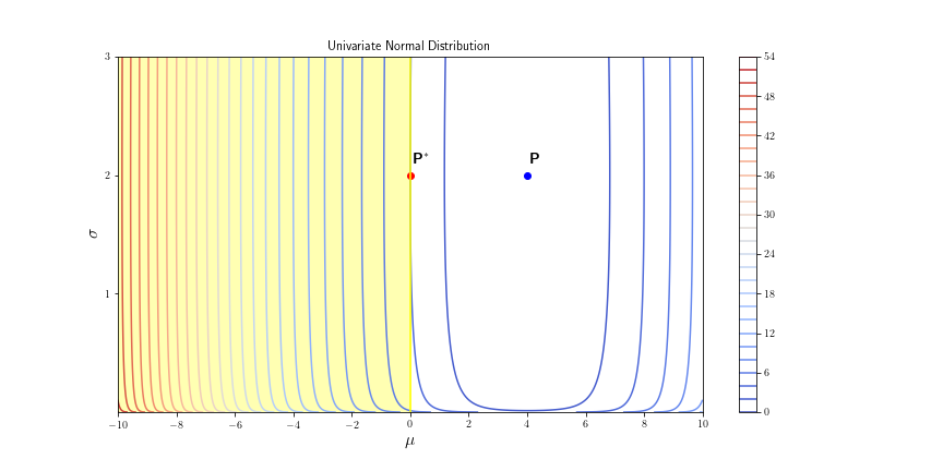
Figure 3: Univariate Normal Distribution, Linear CATE. Each point in the graph represents a normal distribution parametrized by its mean and standard deviation $\mathcal{N}(\mu,\sigma^{2})$. The starting distribution, the experimental is taken to be $\textrm{P}=\mathcal{N}(4,2)$. The contour lines represent the KL divergence with respect to the status quo distribution. The policy-maker’s desired claim is $ATE\geq 0$. The feasible set shaded in yellow represents all univariate normal distributions that satisfy $ATE\leq 0$. When CATE is linear (that is $\tau(x)=\pi X$), the only parameter that contributes to the ATE is the mean $\mu$ so the feasible set is parallel to the $\sigma$ axis. As a result, the least favorable distribution, labelled as $\textrm{P}^{*}$, amounts to a mean shift from $\mu=4$ to $\mu^{*}=\frac{\tilde{\tau}}{\pi}=0$ and no shift in the $\sigma$ parameter.

The KKT conditions imply:

$$\mu^{*} =\mu-\lambda\pi\sigma^{2}$$

$$\sigma^{*} =\sigma$$

$$\lambda =\frac{1}{\pi\sigma^{2}}\left(\mu-\frac{\tilde{\tau}}{\pi}\right)$$

The least favorable distribution amounts to a mean shift of the prescribed magnitude and no change in the variance. Contrast the example above with the case where the CATE is allowed to be quadratic. Proposition 17 still applies, hence the problem can still be formulated as minimizing over the paramteric space $(\mu^{*},\sigma^{*})$. This time though, the variance of the covariate X matters in determining the ATE and the feasible set reflects this.

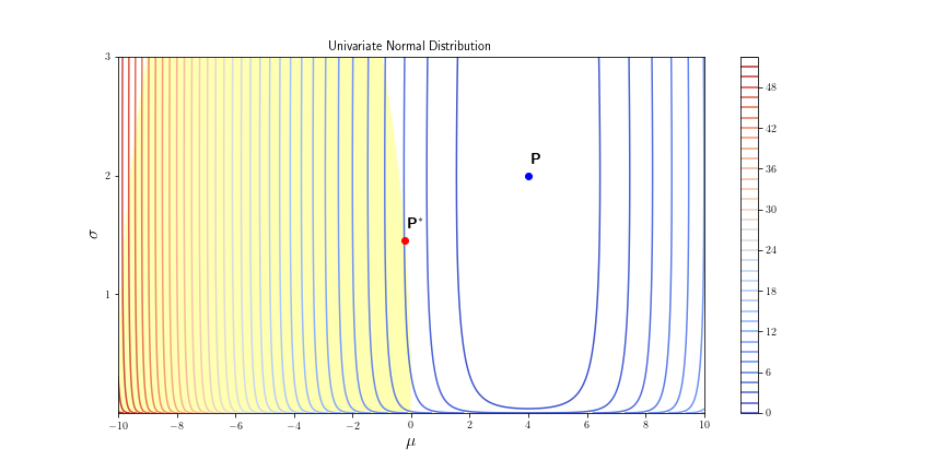
Figure 4: Univariate Normal Distribution: Quadratic CATE. The setting is identical as in Figure 3 but here is quadratic, $\tau(x)=0.8\cdot X^{2}+8\cdot X$. As a result, $ATE(\mu,\sigma)=0.8\cdot(\mu^{2}+\sigma^{2})+8\mu$ so both parameters of the covariate distribution contribute to determining the ATE. The feasible set in yellow has nonflat curvature. The least favorable distribution, labelled as $\textrm{P}^{*}$, features a parameter shift in both the mean and the variance.

Appendix C Constrained Classes

An applied researcher may wish to restrict the class of distributions for problem 1 by imposing additional constraints. For example, they may want to fix the certain moments of the experimental distribution. The computational price to pay for each additional constraint is one additional Lagrange multiplier per constraint as detailed out in Ho [2020]. For example, for a known moment function $q:\mathcal{X}\rightarrow\mathbb{R}$ we want:

$$\int_{\mathcal{X}}q(X)dF_{X}=\int_{\mathcal{X}}q(X)dF_{X}^{\prime}$$

This requirement restricts the space of feasible probability distributions because it asks that the least favorable distribution preserves the additional moment. From the perspective of robustness, the value of the problem $\delta^{*}$ for the constrained problem must be larger or equal than the value for the unconstrained problem. That is:

$$\inf_{dF_{X}^{\prime}:\ dF_{X}^{\prime}\ll dF_{X};P_{X}^{\prime}(\mathcal{X})=1} D_{KL}(F_{X}^{\prime}||F_{X}) \leq \inf_{F_{X}^{\prime}:\ F_{X}^{\prime}\ll F_{X};P_{X}^{\prime}(\mathcal{X})=1} D_{KL}(F_{X}^{\prime}||F_{X})$$

$$s.t.\ \int_{\mathcal{X}}\tau(x)dF_{X}^{\prime}(x)\leq\tilde{\tau} \int_{\mathcal{X}}\tau(x)dF_{X}^{\prime}(x)\leq\tilde{\tau}$$

$$\int_{\mathcal{X}}q(x)dF_{X}^{\prime}(x)=q$$

Assumptions about moment preservation aides the robustness to external validity of a causal claim.
In case of additional constraints the solution to the KL problem takes the form:

$$\frac{dF_{X}^{*}}{dF_{X}}=\frac{\exp(-\lambda(\tau(x)-\tilde{\tau}))\prod_{l=1}^{L}\exp(-\mu_{l}(q(x)-\tilde{q}))}{\int_{\mathcal{X}}\exp(-\lambda(\tau(x)-\tilde{\tau}))\prod_{l=1}^{L}\exp(-\mu_{l}(q(x)-\tilde{q}))}$$

and each Lagrange multiplier can be solved by:

$$\int_{\mathcal{X}}\exp(-\mu_{l}(q(x)-\tilde{q}))(q(x)-\tilde{q})dF_{X}=0$$

For estimation, the additional restrictions result in $L$ many additional parameters, one for each Lagrange multiplier that needs to be computed. One could adapt the estimation framework in Section 3 and have $\theta\in\Theta\subseteq\mathbb{R}^{L+2}$ gathers the original parameters $\alpha$ and $\lambda$ as well as the Lagrange multipliers for the population optimization problem $\mu_{1},\mu_{2},\cdots,\mu_{L}$. At the cost of a more cumbersome notation, all the asymptotic results in Section 3 apply.

Appendix D General $\varphi$-divergence metrics and least favorable closed classes.

In this section I extend the theory of least favorable classes by considering different $\varphi$ divergence measures. To this end I leverage the thorough treatment of $\varphi$ divergences in Christensen and Connault [2019]. The Kullback-Leibler divergence is a special case of a more general construction, known as $\varphi$-divergence. It is introduced below:

Definition 19 ($\varphi$-divergence).

Consider the $\varphi$-divergence between $F_{X}$ and $F_{X}^{\prime}$ given by:

$$D_{\varphi}(F_{X}^{\prime}||F_{X}):=\int\varphi\left(\frac{dF_{X}^{\prime}}{dF_{X}}\right)dF_{X}$$ (19)

where $\varphi$ is a convex function with $\varphi(1)=0$ and $\frac{dF_{X}^{\prime}}{dF_{X}}$ is the Radon-Nikodym derivative of the probability distribution $F_{X}^{\prime}$ with respect to the probability distribution of $F_{X}$, provided that $P_{X}^{\prime}\ll P_{X}$ for the respective measures. For example the choices $\varphi(t)=t\log t$ and $\varphi(t)=\frac{1}{2}|t-1|$ give rise to the KL-divergence and to the total variation divergence (TV) respectively.

There may be a reason to choose a different $\varphi$-divergence metric instead of the KL-divergence. Under suitable conditions, the construction of the proposed robustness metric will change in magnitude, since now the (pseduo)-metric on the space of distributions of the covariates is different. A closed form solution analogous to Lemma 7. The characterization of the $\delta^{*}$, now depends on $\varphi(\cdot)$. In particular it is fully characterized in terms of the Fenchel-conjugate of $\varphi$ and its derivative.

Definition 20 (Fenchel-Conjugate).

Given a topological vector space $X$ and convex function $\varphi:X\rightarrow\mathbb{R}$, the Fenchel-conjugate $\varphi^{*}:X^{*}\rightarrow\mathbb{R}$, defined on the dual space of X, is defined by:

$$\varphi^{*}:x^{*}\mapsto\sup_{x\in X}\langle x^{*},x\rangle-\varphi(x)$$ (20)

Then we can have a generalization of the policy-maker’s problem in Equations (4) and (5) for an arbitrary $\varphi$ divergence in 19:

$$\inf_{P_{X}^{\prime}:\ P_{X}^{\prime}\ll P_{X};P_{X}^{\prime}(\mathcal{X})=1} D_{\varphi}(F_{X}^{\prime}||F_{X})$$ (21)

$$s.t.\ \int_{\mathcal{X}}\tau(x)dF_{X}^{\prime}(x)\leq\tilde{\tau}\$$ (22)

From the KKT Theorem (Theorem 1 in Luenberger [1997]) we can write the problem as:

$$\sup_{\lambda\in\Lambda}\sup_{\xi}\left(\inf_{P_{X}^{\prime}:\ P_{X}^{\prime}\ll P_{X};P_{X}^{\prime}(\mathcal{X})=1}D_{\varphi}(F_{X}^{\prime}||F_{X})+\lambda\int_{\mathcal{X}}(\tau(x)-\tilde{\tau})dF_{X}^{\prime}(x)+\xi\left(\int_{\mathcal{X}}dF_{X}^{\prime}-1\right)\right)$$ (23)

where and $\xi$ is the Lagrange multiplier for integration to unity, $\lambda$ is the Lagrange multiplier for the policy-maker’s claim. Note that $\Lambda=\mathbb{R}_{+}$ or $\mathbb{R}_{-}$ depending on the sign of the policy-maker’s claim. In Equation (9) the Lagrange multiplier $\lambda$ is a 1-dimensional parameter. We can regard the space of probability measures on $\mathcal{X}$ as a subset of the Banach space $\mathcal{M}$ of bounded and finitely additive measures on $\mathcal{X}$. Notice that after fixing the experimental distribution, $D_{KL}(\cdot||F_{X})$ is convex in its first argument. The constraint in Equation (5) can be seen as a map from $\mathcal{M}$ to $\mathbb{R}$. With a careful rewriting we can express the inner problem as:

$$\inf_{P_{X}^{\prime}:\ P_{X}^{\prime}\ll P_{X};P_{X}^{\prime}(\mathcal{X})=1}\int_{\mathcal{X}}\left(\varphi\left(\frac{dF_{X}^{\prime}}{dF_{X}}(x)\right)-\left(-\lambda(\tau(x)-\tilde{\tau})-\xi\right)\frac{dF_{X}^{\prime}}{dF_{X}}(x)\right)dF_{X}(x)-\xi$$

and recognize that, if we can pass the infimum under the integral sign, we can substitute the expression for the Fenchel-conjugate of $\varphi$, switching the sign of the infimum.

$$\inf_{P_{X}^{\prime}:\ P_{X}^{\prime}\ll P_{X};P_{X}^{\prime}(\mathcal{X})=1}\int_{\mathcal{X}}\left(\varphi\left(\frac{dF_{X}^{\prime}}{dF_{X}}(x)\right)-\left(-\lambda(\tau(x)-\tilde{\tau})-\xi\right)\frac{dF_{X}^{\prime}}{dF_{X}}(x)\right)dF_{X}(x)-\xi$$

$$=-\int_{\mathcal{X}}\varphi^{*}(-\lambda(\tau(x)-\tilde{\tau})-\xi)dF_{X}(x)-\xi$$

Substituting this back into the outside problem one obtains:

$$\sup_{\lambda\in\Lambda}\sup_{\xi}\int_{\mathcal{X}}-\varphi^{*}(-\lambda(\tau(x)-\tilde{\tau})-\xi))dF_{X}(x)-\xi$$

which can be maximized with respect to $\xi$ and delivers the first order condition, evaluated at $\xi^{*}$:

$$\int_{\mathcal{X}}\dot{\varphi}^{*}(-\lambda(\tau(x)-\tilde{\tau})-\xi^{*})dF_{X}=1$$ (24)

where $\dot{\varphi}^{*}(\cdot)$ is the derivative of $\varphi^{*}(\cdot)$ with respect to its argument. Observe that the Fenchel-conjugate of $\varphi(t)=t\log(t)$ is given by $\varphi(t^{*})=\exp(t^{*}-1)$. Solving for $\xi^{*}$ here delivers:

$$\xi^{*}=\log\left(\int_{\mathcal{X}}\exp(-\lambda(\tau(x)-\tilde{\tau}-1))dF_{X}(x)\right)$$

Now differentiating with respect to $\lambda$ we obtain

$$\int_{\mathcal{X}}\dot{\varphi}^{*}(-\lambda^{*}(\tau(x)-\tilde{\tau})-\xi^{*})(\tau(x)-\tilde{\tau}+\dot{\xi}^{*}_{\lambda})dF_{X}(x)-\dot{\xi}^{*}_{\lambda}=0$$ (25)

where $\dot{\xi}^{*}_{\lambda}$ is the derivative of $\xi^{*}$ with respect to $\lambda$ and $\lambda^{*}$ is the value that implicitely solves the moment condition in Equation (25). Observe that plugging Equation (24) into Equation (25) allows to simplify it to:

$$\int_{\mathcal{X}}\dot{\varphi}^{*}(-\lambda^{*}(\tau(x)-\tilde{\tau})-\xi^{*})(\tau(x)-\tilde{\tau})dF_{X}=0$$

since the two terms in $\dot{\xi}^{*}_{\lambda}$ cancel out. Moreover, if $\varphi(\cdot)$ is the KL divergence like in the main body of the paper, then

$$\int_{\mathcal{X}}\dot{\varphi}^{*}(-\lambda^{*}(\tau(x)-\tilde{\tau})(\tau(x)-\tilde{\tau})dF_{X}\cdot\exp(-\xi^{*})=0$$

so the additional term $\exp(-\xi^{*})>0$ can be dropped and Equation (25) recovers Equation (9).

Appendix E Proofs

E.1 Proof of Lemma 7

The proof is based on a result that appeared first in Donsker and Varadhan [1975]. More recently Ho [2020] has uses a similar argument to characterize global sensitivity in a Bayesian setting. See 7 First note that, by the Radon-Nikodym theorem, $\frac{dF_{X}^{*}}{dF_{X}}$ exists and $\textrm{supp}\left(\frac{dF_{X}^{\prime}}{dF_{X}}\right)\subset\mathcal{X}$. Recall $\tau(x)=\mathbb{E}[Y_{1}|X=x]-\mathbb{E}[Y_{0}|X=x]$. Then:

$$\inf_{F_{X}^{\prime}:\ P_{X}^{\prime}\ll P_{X};P_{X}^{\prime}(\mathcal{X})=1} D_{KL}(F_{X}^{\prime}||F_{X})$$

$$s.t.\ \int_{\mathcal{X}}\tau(x)dF_{X}^{\prime}(x)=\tilde{\tau}\$$

is equivalent to:

$$\inf_{F_{X}^{\prime}:\ P_{X}^{\prime}\ll P_{X}} D_{KL}(F_{X}^{\prime}||F_{X})$$

$$s.t.\ \int_{\mathcal{X}}\tau(x)\frac{dF_{X}^{\prime}}{dF_{X}}dF_{X}(x)=\tilde{\tau}$$

$$P_{X}^{\prime}(\mathcal{X})=1$$

I adapt a lemma from Donsker and Varadhan [1975]:

Lemma 21.

Let $F_{X}^{*}$ satisfy $\frac{dF_{X}^{*}}{F_{X}}=\frac{\exp(-\lambda(\tau(x)-\tilde{\tau}))}{\int_{\mathcal{X}}\exp(-\lambda(\tau(x)-\tilde{\tau}))dF_{X}}$. For any probability measure $\tilde{F}_{X}$ such that $\tilde{F}_{X}\ll F_{X}$ we have:

$$\log\left(\int_{\mathcal{X}}\exp(-\lambda(\tau(x)-\tilde{\tau}))dF_{X}\right)=-\left[\int_{\mathcal{X}}\lambda(\tau(x)-\tilde{\tau})d\tilde{F}_{X}(x)+D_{KL}(\tilde{F}_{X}||F_{X})\right]+D_{KL}(\tilde{F}_{X}||F_{X}^{*})$$

• First by definition of the KL-divergence we have:

  $$D_{KL}(\tilde{F}_{X}||F_{X}^{*}) =\int_{\mathcal{X}}\log\left(\frac{d\tilde{F}_{X}}{dF_{X}^{*}}\right)d\tilde{F}_{X}$$

  $$=\int_{\mathcal{X}}\log\left(\frac{\frac{d\tilde{F}_{X}}{dF_{X}}}{\frac{dF_{X}^{*}}{dF_{X}}}\right)d\tilde{F}_{X}$$

  $$=\int_{\mathcal{X}}\left(\log\left(\frac{d\tilde{F}_{X}}{dF_{X}}\right)-\log\left(\frac{dF_{X}^{*}}{dF_{X}}\right)\right)d\tilde{F}_{X}$$

  $$=\int_{\mathcal{X}}\log\left(\frac{d\tilde{F}_{X}}{dF_{X}}\right)d\tilde{F}_{X}-\int_{\mathcal{X}}\log\left(\frac{\exp(-\lambda(\tau(x)-\tilde{\tau})}{\int_{\mathcal{X}}\exp(-\lambda(\tau(x)-\tilde{\tau})dF_{X}}\right)d\tilde{F}_{X}$$

  $$=D_{KL}(\tilde{F}_{X}||F_{X})+\int_{\mathcal{X}}\lambda(\tau(x)-\tilde{\tau})d\tilde{F}_{X}+\int_{\mathcal{X}}\log\left(\int_{\mathcal{X}}\exp(-\lambda(\tau(x)-\tilde{\tau}))dF_{X}\right)d\tilde{F}_{X}$$

  $$=D_{KL}(\tilde{F}_{X}||F_{X})+\int_{\mathcal{X}}\lambda(\tau(x)-\tilde{\tau})d\tilde{F}_{X}+\log\left(\int_{\mathcal{X}}\exp(-\lambda(\tau(x)-\tilde{\tau}))dF_{X}\right)$$

  since $\tilde{F}_{X}\ll F_{X}^{*}\ll F_{X}$ and simple algebra. Rearranging we get:

  $$\log\left(\int_{\mathcal{X}}\exp(-\lambda(\tau(x)-\tilde{\tau})dF_{X}\right)=D_{KL}(\tilde{F}_{X}||F_{X}^{*})-\left[\int_{\mathcal{X}}\lambda(\tau(x)-\tilde{\tau})d\tilde{F}_{X}+D_{KL}(\tilde{F}_{X}||F_{X})\right]$$

  ∎

• i) From the lemma above we have:

  $$\log\left(\int_{\mathcal{X}}\exp(-\lambda(\tau(x)-\tilde{\tau}))dF_{X}\right)=D_{KL}(\tilde{F}_{X}||F_{X}^{*})-D_{KL}(\tilde{F}_{X}||F_{X})-\int_{\mathcal{X}}\lambda(\tau(x)-\tilde{\tau})d\tilde{F}_{X}$$

  Now observe that, since the term $\log\left(\int_{\mathcal{X}}\exp(-\lambda(\tau(x)-\tilde{\tau})dF_{X}\right)$ does not depend on $\tilde{F}_{X}$ we must have:

  $$\arg\min_{\tilde{F}_{X}\ll F_{X}}D_{KL}(\tilde{F}_{X}||F_{X}^{*}) =\arg\max_{\tilde{F}_{X}\ll F_{X}}-\int_{X}\lambda(\tau(x)-\tilde{\tau})d\tilde{F}_{X}-D_{KL}(\tilde{F}_{X}||F_{X})$$

  $$=\arg\min_{\tilde{F}_{X}\ll F_{X}}\int_{X}\lambda(\tau(x)-\tilde{\tau})d\tilde{F}_{X}+D_{KL}(\tilde{F}_{X}||F_{X})$$

  but clearly $F_{X}^{*}=\arg\min_{\tilde{F}_{X}\ll F_{X}}D_{KL}(\tilde{F}_{X}||F_{X}^{*})$ so we must have

  $$F_{X}^{*}=\arg\min_{\tilde{F}_{X}\ll F_{X}}D_{KL}(\tilde{F}_{X}||F_{X})+\lambda\int_{X}(\tau(x)-\tilde{\tau})d\tilde{F}_{X}$$

  which is the desired result. ii) Observe that $D_{KL}(F_{X}^{*}||F_{X}^{*})=0$ hence the value of the minimization problem:

  $$\min_{\tilde{F}_{X}\ll F_{X}}D_{KL}(\tilde{F}_{X}||F_{X})+\lambda\int_{X}(\tau(x)-\tilde{\tau})d\tilde{F}_{X} =\min_{\tilde{F}_{X}\ll F_{X}}D_{KL}(\tilde{F}_{X}||F_{X}^{*})-\log\left(\int_{\mathcal{X}}\exp(-\lambda(\tau(x)-\tilde{\tau}))dF_{X}\right)$$

  $$=-\log\left(\int_{\mathcal{X}}\exp(-\lambda(\tau(x)-\tilde{\tau}))dF_{X}\right)$$

  ∎

E.2 Proof of Fact LABEL:fact:equivalence

• First, in this setting $F_{X}^{*}\ll F_{X}$ simply implies $p_{1}=0\implies p_{1}^{*}=0$. Excluding such a trivial case, 12 characterizes $\frac{p_{1}^{*}}{p_{1}}$. First we solve for the Lagrange multiplier $\lambda$ in 12 by noting that:

  $$\tilde{\tau} =\int_{\mathcal{X}}\tau(x)dF_{X}^{*}$$

  $$=\frac{\exp(-\lambda(\tau(1)-\tilde{\tau}))\tau(1)p_{1}+\exp(-\lambda(\tau(0)-\tilde{\tau}))\tau(0)(1-p_{1})}{\exp(-\lambda(\tau(1)-\tilde{\tau}))p_{1}+\exp(-\lambda(\tau(0)-\tilde{\tau}))(1-p_{1})}$$

  rearranging the denominator and since $\tilde{\tau}$ is a constant, we obtain

  $$\quad\exp(-\lambda(\tau(1)-\tilde{\tau}))\tau(1)p_{1}+\exp(-\lambda(\tau(0)-\tilde{\tau}))\tau(0)(1-p_{1})$$

  $$=\exp(-\lambda(\tau(1)-\tilde{\tau}))\tilde{\tau}p_{1}+\exp(-\lambda(\tau(0)-\tilde{\tau}))\tilde{\tau}(1-p_{1})$$

  which gives the condition:

  $$\exp(-\lambda(\tau(1)-\tilde{\tau}))(\tau(1)-\tilde{\tau})p_{1}+\exp(-\lambda(\tau(0)-\tilde{\tau}))(\tau(0)-\tilde{\tau})(1-p_{1})=0$$

  And isolating each side and taking logs we obtain:

  $$-\lambda(\tau(1)-\tau(0))=\log\left(\frac{(\tilde{\tau}-\tau(0))(1-p_{1})}{(\tau(1)-\tilde{\tau})p_{1}}\right)$$

  so that

  $$-\lambda=\frac{1}{(\tau(1)-\tau(0))}\log\left(\frac{(\tilde{\tau}-\tau(0))(1-p_{1})}{(\tau(1)-\tilde{\tau})p_{1}}\right)$$

  Finally, replacing $-\lambda$ in 11 we have:

  $$\frac{p_{1}^{*}}{p_{1}}=\frac{\exp\left(\log\left(\frac{(\tilde{\tau}-\tau(0))(1-p_{1})}{(\tau(1)-\tilde{\tau})p_{1}}\right)\frac{\tau(1)-\tilde{\tau}}{\tau(1)-\tau(0)}\right)}{\exp\left(\log\left(\frac{(\tilde{\tau}-\tau(0))(1-p_{1})}{(\tau(1)-\tilde{\tau})p_{1}}\right)\frac{\tau(1)-\tilde{\tau}}{\tau(1)-\tau(0)}\right)p_{1}+\exp\left(\log\left(\frac{(\tilde{\tau}-\tau(0))(1-p_{1})}{(\tau(1)-\tilde{\tau})p_{1}}\right)\frac{\tau(0)-\tilde{\tau}}{\tau(1)-\tau(0)}\right)(1-p_{1})}$$

  Finally rearranging and combining terms we have:

  $$p_{1}^{*} =\frac{\exp\left(\log\left(\frac{(\tilde{\tau}-\tau(0))(1-p_{1})}{(\tau(1)-\tilde{\tau})p_{1}}\right)\frac{\tau(1)-\tilde{\tau}}{\tau(1)-\tau(0)}\right)p_{1}}{\exp\left(\log\left(\frac{(\tilde{\tau}-\tau(0))(1-p_{1})}{(\tau(1)-\tilde{\tau})p_{1}}\right)\frac{\tau(1)-\tilde{\tau}}{\tau(1)-\tau(0)}\right)p_{1}+\exp\left(\log\left(\frac{(\tilde{\tau}-\tau(0))(1-p_{1})}{(\tau(1)-\tilde{\tau})p_{1}}\right)\frac{\tau(0)-\tilde{\tau}}{\tau(1)-\tau(0)}\right)(1-p_{1})}$$

  $$=\frac{\left(\frac{(\tilde{\tau}-\tau(0))(1-p_{1})}{(\tau(1)-\tilde{\tau})p_{1}}\right)^{\frac{\tau(1)-\tilde{\tau}}{\tau(1)-\tau(0)}}p_{1}}{\left(\frac{(\tilde{\tau}-\tau(0))(1-p_{1})}{(\tau(1)-\tilde{\tau})p_{1}}\right)^{\frac{\tau(1)-\tilde{\tau}}{\tau(1)-\tau(0)}}p_{1}+\left(\frac{(\tilde{\tau}-\tau(0))(1-p_{1})}{(\tau(1)-\tilde{\tau})p_{1}}\right)^{\frac{\tau(0)-\tilde{\tau}}{\tau(1)-\tau(0)}}(1-p_{1})}$$

  $$=\frac{1}{1+\left(\frac{(\tilde{\tau}-\tau(0))(1-p_{1})}{(\tau(1)-\tilde{\tau})p_{1}}\right)^{\frac{\tau(0)-\tilde{\tau}}{\tau(1)-\tau(0)}-\frac{\tau(1)-\tilde{\tau}}{\tau(1)-\tau(0)}}\frac{(1-p_{1})}{p_{1}}}$$

  $$=\frac{1}{1+\left(\frac{(\tilde{\tau}-\tau(0))(1-p_{1})}{(\tau(1)-\tilde{\tau})p_{1}}\right)^{-1}\frac{(1-p_{1})}{p_{1}}}$$

  $$=\frac{1}{1+\frac{\tilde{\tau}-\tau(0)}{\tau(1)-\tau(0)}}$$

  $$=\frac{1}{\frac{\tau(1)-\tau(0)}{\tilde{\tau}-\tau(0)}}$$

  $$=\frac{\tilde{\tau}-\tau(0)}{\tau(1)-\tau(0)}$$

  which, with $\tilde{\tau}=0$, is the solution obtained in Equation (11). ∎

E.3 Proof of Proposition 10

See 10

• First observe that by Lemma 7 and the fact that each $\tau_{m}\in L^{\mathsf{o}}(\mathcal{P}_{X})$ we can construct the sequence of least favorable distributions $F_{m,X}^{*}$ satisfying:

  $$\frac{dF_{m,X}^{*}}{dF_{X}}(x) =\frac{\exp(-\lambda_{m}(\tau(x)-\tilde{\tau}_{m}))}{\int_{\mathcal{X}}\exp(-\lambda_{m}(\tau(x)-\tilde{\tau}_{m}))dF_{X}}$$

  $$\lambda_{m} :\quad\int_{\mathcal{X}}\exp(-\lambda_{m}(\tau(x)-\tilde{\tau}_{m}))(\tau(x)-\tilde{\tau}_{m})dF_{X}=0$$

  ∎

Without loss of generality consider the case where $\tilde{\tau_{b}}=\max_{\mathcal{X}}\tau(x)$. First notice that the sequence of $\lambda_{m}$ defined above is decreasing and unbounded below. To see that it’s decreasing observe that implicitly differentiating $\lambda(\tilde{\tau})$:

$$\frac{\partial}{\partial\tilde{\tau}}\int_{\mathcal{X}}\exp(-\lambda_{m}(\tau(x)-\tilde{\tau}_{m}))(\tau(x)-\tilde{\tau}_{m})dF_{X}(x) =-\frac{\partial{\lambda}}{{\partial\tilde{\tau}}}(\tilde{\tau})\int_{\mathcal{X}}\exp(-\lambda(\tilde{\tau})(\tau(x)-\tilde{\tau}))(\tau(x)-\tilde{\tau})^{2}dF_{X}$$

$$+\lambda(\tilde{\tau})\int_{\mathcal{X}}\exp(-\lambda(\tilde{\tau})(\tau(x)-\tilde{\tau}))(\tau(x)-\tilde{\tau})dF_{X}$$

$$-\int_{\mathcal{X}}\exp(-\lambda(\tilde{\tau})(\tau(x)-\tilde{\tau}))dF_{X}=0$$

by the Dominated Convergence Theorem with envelope $g=\exp(2M)\cdot 2M$. Note that by the definition of $\lambda(\tilde{\tau})$ the second term is equal to 0. Isolating the derivative of $\lambda$ with respect to $\tilde{\tau}$ we have:

$$\frac{\partial{\lambda}}{{\partial\tilde{\tau}}}(\tilde{\tau})=-\frac{\int_{\mathcal{X}}\exp(-\lambda(\tilde{\tau})(\tau(x)-\tilde{\tau}))dF_{X}}{\int_{\mathcal{X}}\exp(-\lambda(\tilde{\tau})(\tau(x)-\tilde{\tau}))(\tau(x)-\tilde{\tau})^{2}dF_{X}}<0$$

so $\lambda(\tilde{\tau})$ is strictly decreasing on its domain. Suppose $\lambda_{m}\geq-B$ for all $m\in N$, with $B>0$. Then:

$$\quad\int_{\mathcal{X}}\exp(-\lambda_{m}(\tau(x)-\tilde{\tau}_{m}))(\tau(x)-\tilde{\tau}_{m})dF_{X}\leq\quad\int_{\mathcal{X}}\exp(B(\tau(x)-\tilde{\tau}_{m}))(\tau(x)-\tilde{\tau}_{m})dF_{X}$$

so taking the limit fro $m\to\infty$, if $P_{X}(\tau(x)\neq\tilde{\tau_{b}})>0$:

$$\lim_{m\to\infty}\int_{\mathcal{X}}\exp(-\lambda_{m}(\tau(x)-\tilde{\tau}_{m}))(\tau(x)-\tilde{\tau}_{m})dF_{X}\leq \lim_{m\to\infty}\int_{\mathcal{X}}\exp(B(\tau(x)-\tilde{\tau}_{m}))(\tau(x)-\tilde{\tau}_{m})dF_{X}(x)$$

$$\leq\int_{\mathcal{X}}\exp(B(\tau(x)-\tilde{\tau}_{b}))(\tau(x)-\tilde{\tau}_{b})dF_{X}(x)<0$$

Then, there exist $m^{*}\in\mathbb{N}$ such that $\int_{\mathcal{X}}\exp(\lambda_{m^{*}}(\tau(x)-\tilde{\tau}_{m^{*}}))(\tau(x)-\tilde{\tau}_{m^{*}})dF_{X}<0$ which is a contradiction. So $\lambda_{m}$ must be unbounded below. Because it’s a strictly decreasing, unbounded below sequence, it must be the case that $\lambda_{m}\rightarrow-\infty$ as $\tilde{\tau}_{m}\rightarrow\tilde{\tau}_{b}$. Now we show convergence in distribution to $\delta_{x_{b}}$. Let $\varphi(\cdot)\in\mathcal{C}_{b}$. We want to show:

$$\lim_{m\to\infty}\int_{\mathcal{X}}\varphi(x)dF_{X,m}^{*}(x)\rightarrow\int_{\mathcal{X}}\varphi(x)\delta_{x_{b}}(x)=\varphi(x_{b})$$

We have:

$$\int_{\mathcal{X}}\varphi(x)dF_{X,m}^{*}(x) =\int_{\mathcal{X}}\varphi(x)\frac{\exp(-\lambda_{m}(\tau(x)-\tilde{\tau}_{b}))dF_{X}(x)}{\int_{\mathcal{X}}\exp(-\lambda_{m}(\tau(x)-\tilde{\tau}_{b}))dF_{X}(x)}$$

$$=\int_{\mathcal{X}}\varphi(x)\frac{\exp(-\lambda_{m}(\tau(x)-\tilde{\tau}_{b}))dF_{X}(x)}{\int_{\mathcal{X}}\exp(-\lambda_{m}(\tau(x)-\tilde{\tau}_{b}))dF_{X}(x)}$$

Noticing that $\lambda_{m}<0$. Consider the change of variables $y=\sqrt{-\lambda_{m}}(x_{b}-x)$. Then $x=x_{b}-\frac{y}{\sqrt{-\lambda_{m}}}$, $dx=-\frac{dy}{\sqrt{-\lambda_{m}}}$. By the change of variable formula:

$$\quad\int_{\mathcal{X}}\varphi(x)\frac{\exp(-\lambda_{m}(\tau(x)-\tilde{\tau}_{b}))f(x)dx}{\int_{\mathcal{X}}\exp(-\lambda_{m}(\tau(x)-\tilde{\tau}_{b}))f(x)dx}$$

$$=\frac{\int_{\mathbb{R}^{k}}\varphi\left(x_{b}-\frac{y}{\sqrt{-\lambda_{m}}}\right)\exp\left(-\lambda_{m}\left(\tau\left(x_{b}-\frac{y}{\sqrt{{-\lambda_{m}}}}\right)-\tau(x_{b})\right)\right)f\left(x_{b}-\frac{y}{\sqrt{{-\lambda_{m}}}}\right)\mathbbm{1}_{\mathcal{Y}(\lambda_{m})}(y)\frac{1}{\sqrt{-\lambda_{m}}}dy}{\int_{\mathbb{R}^{k}}\exp\left(-\lambda_{m}\left(\tau\left(x_{b}-\frac{y}{\sqrt{{-\lambda_{m}}}}\right)-\tau(x_{b})\right)\right)f\left(x_{b}-\frac{y}{\sqrt{{-\lambda_{m}}}}\right)\mathbbm{1}_{\mathcal{Y}(\lambda_{m})}(y)\frac{1}{\sqrt{-\lambda_{m}}}dy}$$

$$=\frac{\int_{\mathbb{R}^{k}}\varphi\left(x_{b}-\frac{y}{\sqrt{-\lambda_{m}}}\right)\exp\left(-\lambda_{m}\left(\tau\left(x_{b}-\frac{y}{\sqrt{{-\lambda_{m}}}}\right)-\tau(x_{b})\right)\right)f\left(x_{b}-\frac{y}{\sqrt{{-\lambda_{m}}}}\right)\mathbbm{1}_{\mathcal{Y}(\lambda_{m})}(y)dy}{\int_{\mathbb{R}^{k}}\exp\left(-\lambda_{m}\left(\tau\left(x_{b}-\frac{y}{\sqrt{{-\lambda_{m}}}}\right)-\tau(x_{b})\right)\right)f\left(x_{b}-\frac{y}{\sqrt{{-\lambda_{m}}}}\right)\mathbbm{1}_{\mathcal{Y}(\lambda_{m})}(y)dy}$$

Note that, if $X$ is compactly supported then $f(x)=0$ outside of a compact set $K\subseteq\mathbb{R}^{k}$ hence. Moreover, if $f(x)<M$ we have the dominating function given by:

$$\varphi\left(x_{b}-\frac{y}{\sqrt{-\lambda_{m}}}\right)\exp\left(-\lambda_{m}\left(\tau\left(x_{b}-\frac{y}{\sqrt{{-\lambda_{m}}}}\right)-\tau(x_{b})\right)\right)f\left(x_{b}-\frac{y}{\sqrt{{-\lambda_{m}}}}\right)\mathbbm{1}_{\mathcal{Y}(\lambda_{m})}(y)dy$$

$$\leq\lVert\varphi\rVert_{\infty}M\mathbbm{1}_{K}(y)$$

on $\mathbb{R}^{k}$ and $\int_{\mathbb{R}^{k}}\lVert\varphi\rVert_{\infty}M\mathbbm{1}_{K}(x)dx=\lVert\varphi\rVert_{\infty}\cdot M\cdot\textrm{vol}(K)<+\infty$. hence the assumptions of the Dominated Convergence theorem hold. Then we have:

$$=\lim_{m\rightarrow\infty}\int_{\mathbb{R}^{k}}\varphi\left(x_{b}-\frac{y}{\sqrt{-\lambda_{m}}}\right)\exp\left(-\lambda_{m}\left(\tau\left(x_{b}-\frac{y}{\sqrt{{-\lambda_{m}}}}\right)-\tau(x_{b})\right)\right)f\left(x_{b}-\frac{y}{\sqrt{{-\lambda_{m}}}}\right)\mathbbm{1}_{\mathcal{Y}(\lambda_{m})}(y)dy$$

$$=\int_{\mathbb{R}^{k}}\lim_{m\rightarrow\infty}\varphi\left(x_{b}-\frac{y}{\sqrt{-\lambda_{m}}}\right)\exp\left(-\lambda_{m}\left(\tau\left(x_{b}-\frac{y}{\sqrt{{-\lambda_{m}}}}\right)-\tau(x_{b})\right)\right)f\left(x_{b}-\frac{y}{\sqrt{{-\lambda_{m}}}}\right)\mathbbm{1}_{\mathcal{Y}(\lambda_{m})}(y)dy$$

Now consider Taylor expanding $\tau(\cdot)$ around $x_{b}$. Because $x_{b}$ is a maximizer, the Jacobian $J_{\tau}(x_{b}):\mathbb{R}^{k}\rightarrow\mathbb{R}$ is the zero matrix, from first order conditions. Hence:

$$\quad\exp\left(-\lambda_{m}\left(\tau\left(x_{b}-\frac{y}{\sqrt{{-\lambda_{m}}}}\right)-\tau(x_{b})\right)\right)$$

$$=\exp\left(-\lambda_{m}\left(\tau(x_{b})-J_{\tau}(x_{b})\left(\frac{y}{\sqrt{{-\lambda_{m}}}}\right)+\frac{1}{2}\cdot\frac{1}{-\lambda_{m}}y^{T}H_{\tau}(x_{b})y-\tau(x_{b})\right)\right)$$

$$=\exp\left(\frac{1}{2}y^{T}H_{\tau}(x_{b})y+o(1)\right)$$

where $H_{\tau}(x_{b})$ is the $k\times k$ Hessian matrix of $\tau$, evaluated at the maximizer $x_{b}$. Moreover:

$$\quad\int_{\mathbb{R}^{k}}\lim_{m\rightarrow\infty}\varphi\left(x_{b}-\frac{y}{\sqrt{-\lambda_{m}}}\right)\exp\left(-\lambda_{m}\left(\tau\left(x_{b}-\frac{y}{\sqrt{{-\lambda_{m}}}}\right)-\tau(x_{b})\right)\right)f\left(x_{b}-\frac{y}{\sqrt{{-\lambda_{m}}}}\right)\mathbbm{1}_{\mathcal{Y}(\lambda_{m})}(y)dy$$

$$=\int_{\mathbb{R}^{k}}\varphi(x_{b})\exp\left(\frac{1}{2}y^{T}H(x_{b})y\right)f(x_{b})dy$$

$$=\varphi(x_{b})\int_{\mathbb{R}^{k}}\exp\left(\frac{1}{2}y^{T}H(x_{b})y\right)f(x_{b})dy$$

Now the denominator can be treated identically to have:

$$\quad\int_{\mathbb{R}^{k}}\lim_{m\rightarrow\infty}\exp\left(-\lambda_{m}\left(\tau\left(x_{b}-\frac{y}{\sqrt{{-\lambda_{m}}}}\right)-\tau(x_{b})\right)\right)f\left(x_{b}-\frac{y}{\sqrt{{-\lambda_{m}}}}\right)\mathbbm{1}_{\mathcal{Y}(\lambda_{m})}(y)dy$$

$$=\int_{\mathbb{R}^{k}}\exp\left(\frac{1}{2}y^{T}H(x_{b})y\right)f(x_{b})dy$$

Now because $x_{b}$ is a maximizer, $H(x_{b})$ is negative definite so the quantities above are finite and the numerator is greater than 0. Finally:

$$\quad\lim_{m\to\infty}\int_{\mathcal{X}}\varphi(x)dF_{X,m}^{*}(x)$$

$$=\lim_{m\to\infty}\frac{\int_{\mathcal{X}}\varphi(x)\exp(-\lambda_{m}(\tau(x)-\tilde{\tau}_{b}))f(x)dx}{\int_{\mathcal{X}}\exp(-\lambda_{m}(\tau(x)-\tilde{\tau}_{b}))f(x)dx}$$

$$=\frac{\lim_{m\to\infty}\int_{\mathcal{X}}\varphi(x)\exp(-\lambda_{m}(\tau(x)-\tilde{\tau}_{b}))f(x)dx}{\lim_{m\to\infty}\int_{\mathcal{X}}\exp(-\lambda_{m}(\tau(x)-\tilde{\tau}_{b}))f(x)dx}$$

$$=\frac{\varphi(x_{b})\int_{\mathbb{R}^{k}}\exp\left(\frac{1}{2}y^{T}H(x_{b})y\right)f(x_{b})dy}{\int_{\mathbb{R}^{k}}\exp\left(\frac{1}{2}y^{T}H(x_{b})y\right)f(x_{b})dy}$$

$$=\varphi(x_{b})$$

Since $\varphi(\cdot)\in\mathcal{C}_{b}$ was arbitrary, by the Portmanteau theorem, $dF_{X,m}^{*}\overset{d}{\rightarrow}\delta_{x_{b}}$.

In the general case where $\mathcal{X}_{b}$ is not a singleton, it seems that the least favorable distribution still concentrates around the uniform distribution on the $\mathcal{X}_{b}$, rather than any distribution like the figure below suggests. I leave this interesting case for future work.

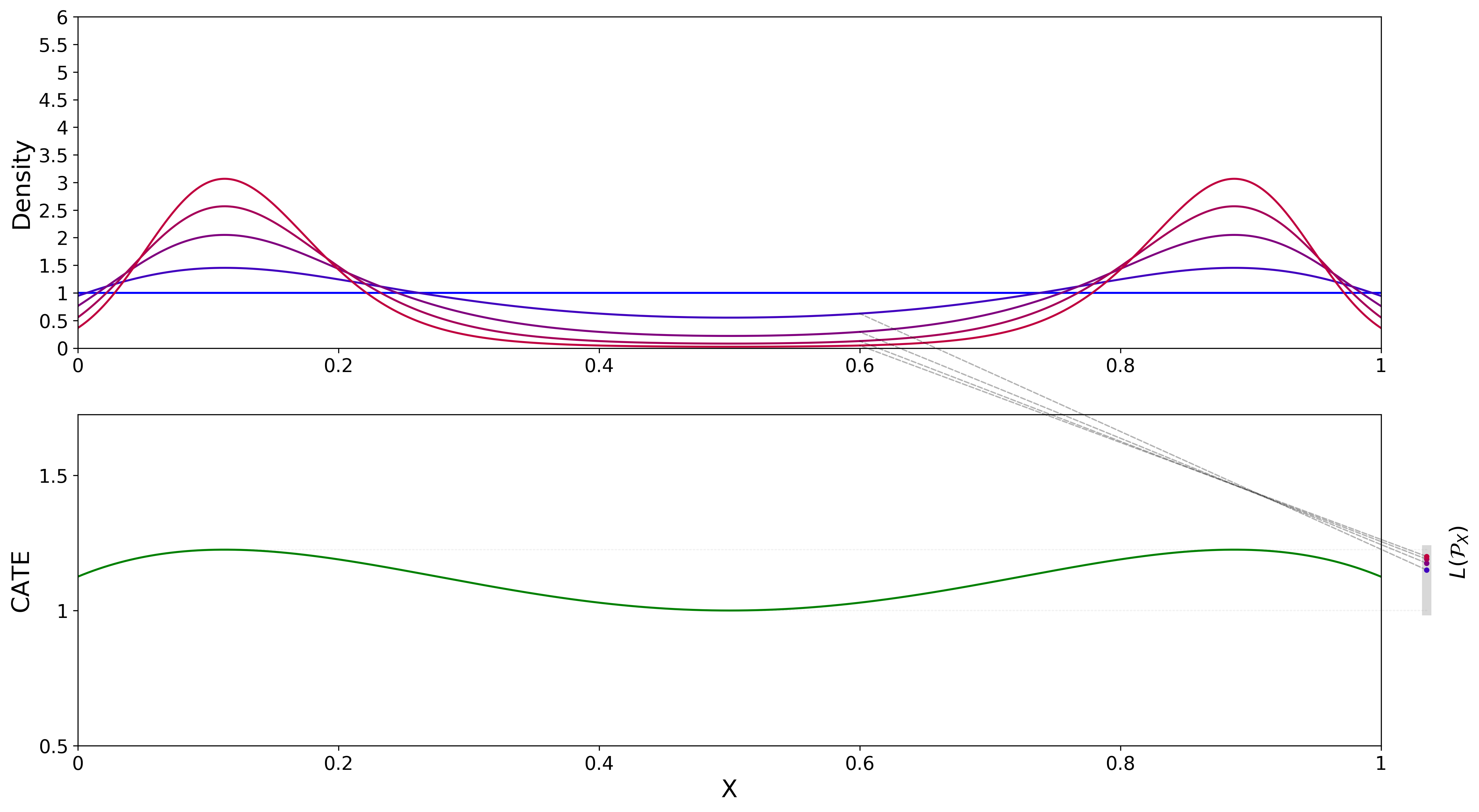
Figure 5: Here $\tau(x)$ is quadratic, experimental distribution is uniform and there are two peaks. It appears that the least favorable distribution concentrates around both peaks.

E.4 Proof of Proposition 17

See 17

• Suppose $\mathcal{X}=\mathbb{R}^{k}$, $X\sim\mathcal{N}(\boldsymbol{\mu},\boldsymbol{\sigma})$ and $\tau(x)=\boldsymbol{x^{T}Ax}+\boldsymbol{x^{T}\beta}+c$. By Lemma 7 the Radon-Nikodym derivative of the least favorable distribution is given by Equation (8) so the distribution of $F_{X}^{*}$ must have density:

$$d\mu_{X}^{*} :=\frac{\exp(-\lambda(\tau(x)-\tilde{\tau}))\frac{\exp\left(-\frac{1}{2}(\boldsymbol{x}-\boldsymbol{\mu})^{T}\boldsymbol{\Sigma}^{-1}(\boldsymbol{x}-\boldsymbol{\mu})\right)}{\sqrt{(2\pi)^{k}\det(\boldsymbol{\Sigma})}}dx}{\displaystyle\int_{\mathcal{X}}\exp(-\lambda(\tau(x)-\tilde{\tau}))\frac{\exp\left(-\frac{1}{2}(\boldsymbol{x}-\boldsymbol{\mu})^{T}\boldsymbol{\Sigma}^{-1}(\boldsymbol{x}-\boldsymbol{\mu})\right)}{\sqrt{(2\pi)^{k}\det(\boldsymbol{\Sigma})}}dx}$$

$$=\frac{\exp(-\lambda(\boldsymbol{x}^{T}\boldsymbol{Ax}+\boldsymbol{x}^{T}\boldsymbol{\beta}+c-\tilde{\tau}))\frac{\exp\left(-\frac{1}{2}(\boldsymbol{x}-\boldsymbol{\mu})^{T}\boldsymbol{\Sigma}^{-1}(\boldsymbol{x}-\boldsymbol{\mu})\right)}{\sqrt{(2\pi)^{k}\det(\boldsymbol{\Sigma})}}dx}{\displaystyle\int_{\mathcal{X}}\exp(-\lambda(\boldsymbol{x}^{T}\boldsymbol{Ax}+\boldsymbol{x}^{T}\boldsymbol{\beta}+c-\tilde{\tau}))\frac{\exp\left(-\frac{1}{2}(\boldsymbol{x}-\boldsymbol{\mu})^{T}\boldsymbol{\Sigma}^{-1}(\boldsymbol{x}-\boldsymbol{\mu})\right)}{\sqrt{(2\pi)^{k}\det(\boldsymbol{\Sigma})}}dx}$$

$$=\frac{\frac{\exp(-\lambda(\boldsymbol{x}^{T}\boldsymbol{Ax}+\boldsymbol{x}^{T}\boldsymbol{\beta}+c-\tilde{\tau})-\frac{1}{2}(\boldsymbol{x}-\boldsymbol{\mu})^{T}\boldsymbol{\Sigma}^{-1}(\boldsymbol{x}-\boldsymbol{\mu}))}{\sqrt{(2\pi)^{k}\det(\boldsymbol{\Sigma})}}dx}{\displaystyle\int_{\mathcal{X}}\frac{\exp(-\lambda(\boldsymbol{x}^{T}\boldsymbol{Ax}+\boldsymbol{x}^{T}\boldsymbol{\beta}+c-\tilde{\tau})-\frac{1}{2}(\boldsymbol{x}-\boldsymbol{\mu})^{T}\boldsymbol{\Sigma}^{-1}(\boldsymbol{x}-\boldsymbol{\mu}))}{\sqrt{(2\pi)^{k}\det(\boldsymbol{\Sigma})}}dx}$$

$$=\frac{\exp(-\lambda(\boldsymbol{x}^{T}\boldsymbol{Ax}+\boldsymbol{x}^{T}\boldsymbol{\beta}+c-\tilde{\tau})-\frac{1}{2}(\boldsymbol{x}-\boldsymbol{\mu})^{T}\boldsymbol{\Sigma}^{-1}(\boldsymbol{x}-\boldsymbol{\mu}))dx}{\displaystyle\int_{\mathcal{X}}\exp(-\lambda(\boldsymbol{x}^{T}\boldsymbol{Ax}+\boldsymbol{x}^{T}\boldsymbol{\beta}+c-\tilde{\tau})-\frac{1}{2}(\boldsymbol{x}-\boldsymbol{\mu})^{T}\boldsymbol{\Sigma}^{-1}(\boldsymbol{x}-\boldsymbol{\mu}))dx}$$

$$=\frac{\exp(-\frac{1}{2}(\boldsymbol{x}-(\boldsymbol{\Sigma}^{-1}+2\lambda\boldsymbol{A})^{-1}(\boldsymbol{\Sigma}^{-1}\boldsymbol{\mu}-\lambda\boldsymbol{\beta}))(\boldsymbol{\Sigma}^{-1}+2\lambda\boldsymbol{A}))(x-(\boldsymbol{\Sigma}^{-1}+2\lambda\boldsymbol{A})^{-1}(\boldsymbol{\Sigma}^{-1}\boldsymbol{\mu}-\lambda\boldsymbol{\beta}))dx}{\displaystyle\int_{\mathcal{X}}\exp(-\frac{1}{2}(x-(\boldsymbol{\Sigma}^{-1}+2\lambda\boldsymbol{A})^{-1}(\boldsymbol{\Sigma}^{-1}\boldsymbol{\mu}-\lambda\boldsymbol{\beta}))(\boldsymbol{\Sigma}^{-1}+2\lambda\boldsymbol{A}))(x-(\boldsymbol{\Sigma}^{-1}+2\lambda\boldsymbol{A})^{-1}(\boldsymbol{\Sigma}^{-1}\boldsymbol{\mu}-\lambda\boldsymbol{\beta}))dx}$$

$$\times\frac{\exp(\lambda c+\lambda\tilde{\tau}-\frac{1}{2}\boldsymbol{\mu}^{T}\boldsymbol{\Sigma}^{-1}\boldsymbol{\mu}-\frac{1}{2}(\boldsymbol{\Sigma}^{-1}\boldsymbol{\mu}-\lambda\boldsymbol{\beta})(\boldsymbol{\Sigma}^{-1}+2\lambda\boldsymbol{\beta})^{-1}(\boldsymbol{\Sigma}^{-1}\boldsymbol{\mu}-\lambda\boldsymbol{\beta}))}{\exp(\lambda c+\lambda\tilde{\tau}-\frac{1}{2}\boldsymbol{\mu}^{T}\boldsymbol{\Sigma}^{-1}\boldsymbol{\mu}-\frac{1}{2}(\boldsymbol{\Sigma}^{-1}\boldsymbol{\mu}-\lambda\boldsymbol{\beta})(\boldsymbol{\Sigma}^{-1}+2\lambda\boldsymbol{\beta})^{-1}(\boldsymbol{\Sigma}^{-1}\boldsymbol{\mu}-\lambda\boldsymbol{\beta}))}$$

$$=\frac{\exp(-\frac{1}{2}(\boldsymbol{x}-(\boldsymbol{\Sigma}^{-1}+2\lambda\boldsymbol{A})^{-1}(\boldsymbol{\Sigma}^{-1}\mu-\lambda\boldsymbol{\beta}))(\boldsymbol{\Sigma}^{-1}+2\lambda\boldsymbol{A}))(x-(\boldsymbol{\Sigma}^{-1}+2\lambda\boldsymbol{A})^{-1}(\boldsymbol{\Sigma}^{-1}\boldsymbol{\mu}-\lambda\boldsymbol{\beta}))dx}{\displaystyle\int_{\mathcal{X}}\exp(-\frac{1}{2}(\boldsymbol{x}-(\boldsymbol{\Sigma}^{-1}+2\lambda\boldsymbol{A})^{-1}(\boldsymbol{\Sigma}^{-1}\boldsymbol{\mu}-\lambda\boldsymbol{\beta}))(\boldsymbol{\Sigma}^{-1}+2\lambda\boldsymbol{A}))(\boldsymbol{x}-(\boldsymbol{\Sigma}^{-1}+2\lambda\boldsymbol{A})^{-1}(\boldsymbol{\Sigma}^{-1}\boldsymbol{\mu}-\lambda\boldsymbol{\beta}))dx}$$

from which we can recognize the form of the normal distribution with mean $\boldsymbol{\mu}^{*}$ and variance covariance matrix $\boldsymbol{\Sigma}^{*}$. The steps above follow from completing the square and from the properties of $\exp(\cdot)$. ∎

E.5 Proof of Proposition 11

See 11

Let $F_{r}=(1-r)F_{0}+rH$ for an arbitrary distribution $H$ that satisfies unconfounded-ness. Then $F_{r}$ is a distribution because it’s a convex combination of two distributions, and it satisfies unconfounded-ness. Therefore we can refer to the identification results:

$$\mathbb{E}_{F_{r}}[Y_{1}|X] =\mathbb{E}_{F_{r}}[Y|D=1,X]$$

$$\mathbb{E}_{F_{r}}[Y_{0}|X] =\mathbb{E}_{F_{r}}[Y|D=0,X]$$

and derive the distributional derivative of $\mathbb{E}_{F_{r}}[Y|D=1,X]-\mathbb{E}_{F_{r}}[Y|D=0,X]$ with respect to $r$ and evaluate it at $r=0$. Alternatively one may start with the propensity score weighting identification result below:

$$\mathbb{E}_{F_{r}}\left[\frac{Y\cdot D}{\pi_{F_{r}}(X)}-\frac{Y\cdot(1-D)}{\pi_{F_{r}}(X)}\Bigg{|}X\right]=\mathbb{E}_{F_{r}}[Y_{1}-Y_{0}|X]$$

and proceed as above to derive the distributional derivative of $\mathbb{E}_{F}[g(W,\theta,\gamma(F_{r}))]$. The second approach is more cumbersome so we present the proof for the regression adjustment method but note that both would be valid approaches to find the nonparametric influence function. Computing the derivative of the moment condition with respect to $r$ and evaluating it at $r=0$ we have:

$$\frac{d\mathbb{E}[g(W,\theta,\gamma(F_{r}))]}{dr}\Bigg{|}_{r=0} =\frac{d}{dr}\mathbb{E}\begin{bmatrix}\exp(-\lambda_{0}(\gamma_{1,F_{r}}(x)-\gamma_{0,F_{r}}(x)-\tilde{\tau}))-\nu]\\ \exp\left(-\lambda_{0}(\gamma_{1,F_{r}}(x)-\gamma_{0,F_{r}}(x)-\tilde{\tau})\right)(\gamma_{1,F_{r}}(x)-\gamma_{0,F_{r}}(x)-\tilde{\tau})]\end{bmatrix}\Bigg{|}_{r=0}$$

$$= \int_{\mathcal{X}}\frac{d}{dr}\begin{bmatrix}\exp\left(-\lambda_{0}\cdot(\gamma_{1,F_{r}}(x)-\gamma_{0,F_{r}}(x)-\tilde{\tau})\right)\\ \exp\left(-\lambda_{0}\cdot(\gamma_{1,F_{r}}(x)-\gamma_{0,F_{r}}(x)-\tilde{\tau})\right)(\gamma_{1,F_{r}}(x)-\gamma_{0,F_{r}}(x)-\tilde{\tau})\end{bmatrix}f_{0}(x)dx\Bigg{|}_{r=0}$$

$$= \int_{\mathcal{X}}\begin{bmatrix}\exp\left(-\lambda_{0}\cdot(\gamma_{1,F_{r}}(x)-\gamma_{0,F_{r}}(x)-\tilde{\tau})\right)\cdot(-\lambda_{0})\\ \exp\left(-\lambda_{0}\cdot(\gamma_{1,F_{r}}(x)-\gamma_{0,F_{r}}(x)-\tilde{\tau})\right)\cdot(1-\lambda\cdot(\gamma_{1,F_{r}}(x)-\gamma_{0,F_{r}}(x)-\tilde{\tau}))\end{bmatrix}$$

$$\times \frac{\partial}{\partial r}(\gamma_{1,F_{r}}(x)-\gamma_{0,F_{r}}(x))f_{0}(x)dx$$

In order to characterize the contribution of the functional we have:

$$\ \frac{\partial}{\partial r}(\gamma_{1,F_{r}}(x)-\gamma_{0,F_{r}}(x))$$

$$=\frac{\partial}{\partial r}\int_{\mathcal{Y}}\frac{y}{\int_{\mathcal{Y}}(1-r)dF_{0}(y,1,x)+rdH(y,1,x)}((1-r)dF(y,1,x)+rdH(y,1,x))$$

$$-\frac{\partial}{\partial r}\int_{\mathcal{Y}}\frac{y}{\int_{\mathcal{Y}}(1-r)dF_{0}(y,0,x)+rdH(y,0,x)}((1-r)dF(y,0,x)+rdH(y,0,x))$$

$$=\int_{\mathcal{Y}}y\cdot\frac{[dH(y,1,x)-dF_{0}(y,1,x)]\int_{\mathcal{Y}}(1-r)dF_{0}(y,1,x)+rdH(y,1,x)-\int_{\mathcal{Y}}[dH(y,1,x)-dF_{0}(y,1,x)]((1-r)dF_{0}(y,1,x)-dH(y,1,x))}{\left(\int_{\mathcal{Y}}(1+r)dF_{0}(y,1,x)+rdH(y,1,x)\right)^{2}}$$

$$-\int_{\mathcal{Y}}y\cdot\frac{[dH(y,0,x)-dF_{0}(y,0,x)]\int_{\mathcal{Y}}(1-r)dF_{0}(y,0,x)+rdH(y,0,x)-\int_{\mathcal{Y}}[dH(y,0,x)-dF_{0}(y,0,x)]((1-r)dF_{0}(y,0,x)-dH(y,0,x))}{\left(\int_{\mathcal{Y}}(1+r)dF_{0}(y,0,x)+rdH(y,0,x)\right)^{2}}$$

Below $f_{0}(d,x)=\int_{\mathcal{Y}}dF_{0}(y,d,x)$ and the same holds for $h(\cdot)$. Evaluating this expression at $r=0$ one obtains:

$$\int y\cdot\frac{dH(y,1,x)}{f_{0}(1,x)}-\int y\cdot\frac{h(1,x)\cdot dF_{0}(y,1,x)}{f_{0}(1,x)^{2}}-\int y\cdot\frac{dH(y,0,x)}{f_{0}(0,x)}+\int y\cdot\frac{h(0,x)\cdot dF_{0}(y,0,x)}{f_{0}(0,x)^{2}}$$

Combining this with the derivative of the moment condition with respect to the $\gamma$ we have:

$$\frac{d\mathbb{E}[g(W,\theta,\gamma(F_{r}))]}{dr} =\int_{\mathcal{Y}\times\{0,1\}\times\mathcal{X}}\begin{bmatrix}\exp\left(-\lambda\cdot(\gamma_{1,F_{0}}(x)-\gamma_{0,F_{0}}(x)-\tilde{\tau})\right)\cdot(-\lambda)\\ \exp\left(-\lambda\cdot(\gamma_{1,F_{0}}(x)-\gamma_{0,F_{0}}(x)-\tilde{\tau})\right)\cdot(1-\lambda\cdot(\gamma_{1,F_{0}}(x)-\gamma_{0,F_{0}}(x)-\tilde{\tau}))\end{bmatrix}$$

$$\times\left(\frac{d(y-\gamma_{1,F_{0}}(x))}{\pi_{F_{0}}(x)}-\frac{(1-d)(y-\gamma_{0,F_{0}}(x))}{1-\pi_{F_{0}}(x)}\right)dH(y,d,x)$$

or $\frac{d\mathbb{E}[g(W,\theta,\gamma(F_{r}))]}{dr}=\int_{\mathcal{Y}\times\{0,1\}\times\mathcal{X}}\phi(w,\theta,\gamma(F_{0}),\alpha(F_{0}))dH(w)$ for

$$\phi(w,\theta,\gamma,\alpha) =\begin{bmatrix}\exp\left(-\lambda\cdot(\gamma_{1,F_{0}}(x)-\gamma_{0,F_{0}}(x)-\tilde{\tau})\right)\cdot(-\lambda)\\ \exp\left(-\lambda\cdot(\gamma_{1,F_{0}}(x)-\gamma_{0,F_{0}}(x)-\tilde{\tau})\right)\cdot(1-\lambda\cdot(\gamma_{1,F_{0}}(x)-\gamma_{0,F_{0}}(x)-\tilde{\tau}))\end{bmatrix}$$

$$\times\left(\frac{d(y-\gamma_{1,F_{0}}(x))}{\pi_{F}(x)}-\frac{(1-d)(y-\gamma_{0,F_{0}}(x))}{1-\pi_{F}(x)}\right)$$

$$=\begin{bmatrix}\exp\left(-\lambda\cdot(\gamma_{1,F_{0}}(x)-\gamma_{0,F_{0}}(x)-\tilde{\tau})\right)\cdot(-\lambda)\\ \exp\left(-\lambda\cdot(\gamma_{1,F_{0}}(x)-\gamma_{0,F_{0}}(x)-\tilde{\tau})\right)\cdot(1-\lambda\cdot(\gamma_{1,F_{0}}(x)-\gamma_{0,F_{0}}(x)-\tilde{\tau}))\end{bmatrix}$$

$$\times\left(\begin{bmatrix}\alpha_{1,F_{0}}(x)\\ \alpha_{0,F_{0}}(x)\end{bmatrix}^{T}\begin{bmatrix}d(y-\gamma_{1,F_{0}}(x))\\ (1-d)(y-\gamma_{0,F_{0}}(x))\end{bmatrix}\right)$$

and $\alpha_{F_{0}}(X):=\begin{bmatrix}\alpha_{1,F_{0}}(x)\\ \alpha_{0,F_{0}}(x)\end{bmatrix}=\begin{bmatrix}\frac{1}{\pi_{F_{0}}(X)}\\ \frac{1}{1-\pi_{F_{0}}(X)}\end{bmatrix}$. Note that above $\phi(\cdot)$ is the Riesz representer of the linear functional $\frac{d\mathbb{E}[g(W,\theta,\gamma(F_{r}))]}{dr}\Bigg{|}_{r=0}:\mathcal{H}\rightarrow\mathbb{R}^{2}$ which maps $H$ to $\mathbb{R}^{2}$.

Observe that $\mathbb{E}_{F_{0}}[\phi(W,\theta,\gamma_{0}(X),\alpha_{0}(X)]=0$ by the law of iterated expectations. Moreover, for any distribution $F$, $\mathbb{E}_{F}\left[\frac{D(Y-\mathbb{E}_{F}[Y|D=1,X])}{\pi_{F}(X)}-\frac{(1-D)(Y-\mathbb{E}_{F}[Y|D=0,X]}{1-\pi_{F}(X)}\Bigg{|}X\right]=0$. ∎

E.6 Proof of Proposition 12

See 12

• To show that they are Neyman orthogonal we verify the conditions for Theorem 1 in Chernozhukov et al. [2020] in the Appendix. Let $\gamma_{1,F}(X),\gamma_{0,0}(X)$ denote $\mathbb{E}_{F}[Y|D=1,X],\mathbb{E}_{F}[Y|D=0,X]$ respectively. i) Equation (15) holds. This has been verified above.
  ii) $\int_{\mathcal{Y}_{0}\times\mathcal{Y}_{1}\times\mathcal{X}}\phi(w,\gamma(F_{r}),\theta,\alpha(F_{r}))F_{r}(dw)=0$ for all $r\in[0,\tilde{r})$:
  This is immediate by the law of iterated expectations

  $$\mathbb{E}_{F_{r}}[\phi(W,\gamma(F_{r}),\theta,\alpha(F_{r})] =\mathbb{E}_{F_{r}}\left[\mathbb{E}_{F_{r}}[\phi(W,\gamma(F_{r}),\theta,\alpha(F_{r})|X]\right]$$

  $$=\mathbb{E}_{F_{r}}\left[v(X)\cdot\mathbb{E}_{F_{r}}\left[\left(\frac{d(y-\gamma_{1,F_{r}}(X))}{\pi_{F_{r}}(X)}-\frac{(1-d)(y-\gamma_{1,F_{r}}(X))}{1-\pi_{F_{r}}(X)}\right)\Bigg{|}X\right]\right]$$

  $$=\mathbb{E}_{F_{r}}[v(X)\cdot 0]$$

  $$=0$$

  for $v(X)=\begin{bmatrix}\exp\left(-\lambda\cdot(\gamma_{1,F_{r}}(x)-\gamma_{0,F_{r}}(x)-\tilde{\tau})\right)\cdot(-\lambda)\\ \exp\left(-\lambda\cdot(\gamma_{1,F_{r}}(x)-\gamma_{0,F_{r}}(x)-\tilde{\tau})\right)\cdot(1-\lambda\cdot(\gamma_{1,F_{r}}(x)-\gamma_{0,F_{r}}(x)-\tilde{\tau}))\end{bmatrix}$
  iii) $\int_{\mathcal{Y}_{0}\times\mathcal{Y}_{1}\times\mathcal{X}}\phi(w,\gamma(F_{r}),\theta,\alpha(F_{r}))H(dw)$ and $\int_{\mathcal{Y}_{0}\times\mathcal{Y}_{1}\times\mathcal{X}}\phi(w,\gamma(F_{r}),\theta,\alpha(F_{r}))F_{0}(dw)$ are continuous at $r=0$. For a given $H$, we show that function $b:r\mapsto\int_{\mathcal{Y}_{0}\times\mathcal{Y}_{1}\times\mathcal{X}}\phi(w,\gamma(F_{r}),\theta,\alpha(F_{r}))H(dw)$ is continuous at $r=0$. Take a sequence $r_{m}\rightarrow r=0$, then $\phi_{n}(w):=\phi(w,\gamma(F_{r_{m}}),\theta,\alpha(F_{r_{m}}))$ converges $H$-almost everywhere to $\phi_{0}(w):=\phi(w,\gamma(F_{0}),\theta,\alpha(F_{0}))$. Moreover we have $\phi_{m}(w)\leq F(w)$ for all $m\in\mathbb{N}$ with $F\in L^{1}(H)$. By the dominated convergence theorem we have: $b(r_{m})\rightarrow b(0)$ which is the desired result.
  An analogous argument applies to the integral with respect to $F_{0}$. As a consequence of Theorems 1,2 and 3 in Chernozhukov et al. [2020] $\psi(w,\gamma,\theta,\alpha)$ is Neyman orthogonal. We can also verify Neyman orthogonality directly from the form of the $\bar{\psi}$ function. In particular:

  $$\quad\ \frac{\partial}{\partial r}\mathbb{E}[\psi(W,\theta,\gamma_{F_{r}},\alpha_{F_{r}})]\Bigg{|}_{r=0}$$

  $$=\frac{\partial}{\partial r}\mathbb{E}[g(W,\theta,\gamma)+\phi(W,\theta,\gamma,\alpha)]\Bigg{|}_{r=0}$$

  $$=\mathbb{E}\Bigg{[}\frac{\partial}{\partial r}\begin{bmatrix}\exp\left(-\lambda_{0}\cdot(\gamma_{1,F_{r}}(X)-\gamma_{0,F_{r}}(X)-\tilde{\tau})\right)\\ \exp\left(-\lambda_{0}\cdot(\gamma_{1,F_{r}}(X)-\gamma_{0,F_{r}}(X)-\tilde{\tau})\right)(\gamma_{1,F_{r}}(X)-\gamma_{0,F_{r}}(X)-\tilde{\tau})\end{bmatrix}$$

  $$+\frac{\partial}{\partial r}\Bigg{(}\begin{bmatrix}\exp\left(-\lambda\cdot(\gamma_{1,F_{r}}(X)-\gamma_{0,F_{r}}(X)-\tilde{\tau})\right)\cdot(-\lambda)\\ \exp\left(-\lambda\cdot(\gamma_{1,F_{r}}(X)-\gamma_{0,F_{r}}(X)-\tilde{\tau})\right)\cdot(1-\lambda\cdot(\gamma_{1,F_{r}}(X)-\gamma_{0,F_{r}}(X)-\tilde{\tau}))\end{bmatrix}$$

  $$\times\left(\frac{D(Y-\gamma_{1,F_{r}}(X))}{\pi_{F_{r}}(X)}-\frac{(1-D)(Y-\gamma_{0,F_{r}}(X))}{1-\pi_{F_{r}}(X)}\right)\Bigg{)}\Bigg{]}$$

  $$=\mathbb{E}\Bigg{[}\begin{bmatrix}\exp\left(-\lambda\cdot(\gamma_{1,F_{0}}(X)-\gamma_{0,F_{0}}(X)-\tilde{\tau})\right)\cdot(-\lambda)\\ \exp\left(-\lambda\cdot(\gamma_{1,F_{0}}(X)-\gamma_{0,F_{0}}(X)-\tilde{\tau})\right)\cdot(1-\lambda\cdot(\gamma_{1,F_{0}}(X)-\gamma_{0,F_{0}}(X)-\tilde{\tau}))\end{bmatrix}$$

  $$\times\Bigg{(}\frac{\partial\gamma_{1,F_{r}}(X)}{\partial r}-\frac{\partial\gamma_{0,F_{r}}(X)}{\partial r}\Bigg{)}\Bigg{|}_{r=0}$$

  $$-\begin{bmatrix}\exp\left(-\lambda\cdot(\gamma_{1,F_{0}}(X)-\gamma_{0,F_{0}}(X)-\tilde{\tau})\right)\cdot(-\lambda)\\ \exp\left(-\lambda\cdot(\gamma_{1,F_{0}}(X)-\gamma_{0,F_{0}}(X)-\tilde{\tau})\right)\cdot(1-\lambda\cdot(\gamma_{1,F_{0}}(X)-\gamma_{0,F_{0}}(X)-\tilde{\tau}))\end{bmatrix}$$

  $$\times\Bigg{(}\frac{D}{\pi_{F_{0}}(X)}\cdot\frac{\partial\gamma_{1,F_{r}}(X)}{\partial r}\Bigg{|}_{r=0}-\frac{(1-D)}{1-\pi_{F_{0}}(X)}\cdot\frac{\partial\gamma_{0,F_{r}}(X)}{\partial r}\Bigg{|}_{r=0}\Bigg{)}$$

  $$+\begin{bmatrix}\exp\left(-\lambda\cdot(\gamma_{1,F_{0}}(X)-\gamma_{0,F_{0}}(X)-\tilde{\tau})\right)\cdot(\lambda)^{2}\\ \exp\left(-\lambda\cdot(\gamma_{1,F_{0}}(X)-\gamma_{0,F_{0}}(X)-\tilde{\tau})\right)\cdot(-\lambda)\cdot(2-\lambda\cdot(\gamma_{1,F_{0}}(X)-\gamma_{0,F_{0}}(X)-\tilde{\tau}))\end{bmatrix}$$

  $$\times\Bigg{(}\frac{\partial\gamma_{1,F_{r}}(X)}{\partial r}-\frac{\partial\gamma_{0,F_{r}}(X)}{\partial r}\Bigg{)}\Bigg{|}_{r=0}\times\left(\frac{D(Y-\gamma_{1,F_{0}}(x))}{\pi_{F_{0}}(X)}-\frac{(1-D)(Y-\gamma_{0,F_{0}}(X))}{1-\pi_{F_{0}}(X)}\right)\Bigg{]}$$

  $$+\begin{bmatrix}\exp\left(-\lambda\cdot(\gamma_{F_{0}}(X)-\tilde{\tau})\right)\cdot(-\lambda)\\ \exp\left(-\lambda\cdot(\gamma_{1,F_{0}}(X)-\gamma_{0,F_{0}}(X)-\tilde{\tau})\right)\cdot(1-\lambda\cdot(\gamma_{1,F_{0}}(X)-\gamma_{0,F_{0}}(X)-\tilde{\tau}))\end{bmatrix}$$

  $$\times\Bigg{(}D(Y-\gamma_{1,F_{0}}(X))\cdot\frac{\partial}{\partial r}\left(\frac{1}{\pi_{F_{r}}(X)}\right)\Bigg{|}_{r=0}-(1-D)(Y-\gamma_{0,F_{0}}(X))\cdot\frac{\partial}{\partial r}\left(\frac{1}{1-\pi_{F_{r}}(X)}\right)\Bigg{|}_{r=0}\Bigg{)}$$

  $$=0$$

  The last equality follows by the law of iterated expectations. The first and second term cancel out since $\mathbb{E}\left[\frac{D}{\pi_{F_{0}}(X)}\Big{|}X\right]=1,\mathbb{E}\left[\frac{1-D}{1-\pi_{F_{0}}(X)}\Big{|}X\right]=1$. The third term is 0 because the nonparametric influence function is centered at 0 conditional on $X$. Moreover, $\mathbb{E}\left[D(Y-\mathbb{E}[Y|D=1,X]\Big{|}X\right]=0$ and $\mathbb{E}\left[(1-D)(Y-\mathbb{E}[Y|D=0,X]\Big{|}X\right]=0$ so whenever $\frac{\partial}{\partial r}\left(\frac{1}{\pi_{F_{r}}(X)}\right)\Big{|}_{r=0}$ and $\frac{\partial}{\partial r}\left(\frac{1}{1-\pi_{F_{r}}(X)}\right)\Big{|}_{r=0}$ are integrable, the fourth term is also 0, since they are measurable with respect to $\sigma(X)$. So $\frac{\partial}{\partial r}\mathbb{E}[\psi(W,\theta,\gamma_{F_{r}},\alpha_{F_{r}})]\Big{|}_{r=0}=0$. Observe that this result implies Neyman orthogonality with respect to the $\gamma$ and $\alpha$ functions separately as well. To show the Neyman orthogonality with respect to $\gamma$ and to set up the further results contained in Theorem 3 in Chernozhukov et al. [2020], we build the following construction. Consider the linear space of square integrable functions of $X$ (with respect to some dominating measure), denoted as $\Gamma=L^{2}(\mathcal{X})$. $\mathcal{H}$ is the closed set of distributions which is a closed subset of the Banach space $L^{1}(\mathcal{Y}_{0}\times\mathcal{Y}_{1}\times\mathcal{X},\mu)$ under some appropriate dominating measure $\mu$. Denote the Hadamard differential of the conditional mean function at $F_{0}$ as $\frac{\partial{\gamma(F_{r})}}{\partial r}:\mathcal{H}\rightarrow\Gamma$. Denote the Hadamard differential for $\bar{\psi}(\gamma(F_{r}),\alpha_{0},\theta)$ at $F_{0}$ as $\frac{\partial\mathbb{E}[\psi(W,\gamma(F_{r}),\alpha(F_{r}),\theta)]}{\partial r}:\mathcal{H}\rightarrow\mathbb{R}^{2}$. Finally denote the Hadamard differential of $\bar{\psi}(\gamma,\theta)$ with respect to $\gamma$ as $\frac{\partial\bar{\psi}(\gamma,\alpha,\theta)}{\partial\gamma}:\Gamma\rightarrow\mathbb{R}^{2}$. Then the following diagram commutes by Proposition 20.9 in Van der Vaart [2000].

  By Neymann orthogonality with respect to the distribution $F_{r}$, $\frac{\partial\mathbb{E}[\psi(W,\gamma(F_{r}),\alpha_{0},\theta)]}{\partial r}\equiv 0$. $\frac{\partial\bar{\psi}(\gamma,\theta)}{\partial\gamma}$ is onto $\Gamma$ which satisfies Chernozhukov et al. [2020] Theorem 3 condition iv). Then, by linearity of the Hadamard derivative and the commutativity of the above diagram it must be the case that $\frac{\partial\bar{\psi}(W,\gamma,\alpha_{0},\theta)}{\partial\gamma}\equiv 0$. That is, the Hadamard derivative is the 0 function from $\Gamma\rightarrow\mathbb{R}^{2}$. Note that this is the case because $\frac{\partial\gamma(F_{r})}{\partial r}$ is onto $L^{2}(\mathcal{X})$. According to the above calculations we have, for $\delta_{H}:=\frac{\partial\gamma_{1,F_{r}}}{\partial r}-\frac{\partial\gamma_{0,F_{r}}}{\partial r}\Big{|}_{r=0}\in L^{2}(\mathcal{X})$. Then as specified above: $\frac{\partial\mathbb{E}[\bar{\psi}(\theta,\alpha_{0},\gamma)]}{\partial\gamma}(\delta_{H})$ is a linear map from $L^{2}(X)\to\mathbb{R}^{2}$ in $\delta_{H}$. In particular it maps to $0\in\mathbb{R}^{2}$ for any $\delta_{H}(X)$, so it’s the 0 map. Hence we verified Neyman orthogonality with respect to $\gamma$ directly. ∎

E.7 Proof of Theorem 13

Lemma 22.

For $\bar{\psi}(\theta,\gamma,\alpha)=\mathbb{E}[\psi(w,\theta,\gamma,\alpha)]$ we have:

i) $\bar{\psi}(\gamma,\alpha_{0},\theta_{0})$ is twice continuously Frechet differentiable in a neighborhood of $\gamma_{0}$.

ii) If $\Lambda$ is bounded then $\forall\theta\in\Theta$, $\bar{\psi}(\gamma,\alpha_{0},\theta)\leq\bar{C}\lVert\gamma-\gamma_{0}\rVert^{2}_{L_{2}}$.

• Endow the spaces $\Gamma$ with the $L^{2}(\mathcal{X},\mu)$ norm and $\mathbb{R}^{2}$ with the standard Euclidean norm $\lVert\cdot\rVert$. We directly compute the directional derivative of $\bar{\psi}(\theta,\gamma,\alpha)$ with respect to $\gamma$.

  $$\frac{\partial}{\partial r}\bar{\psi}(\gamma,\theta,\alpha_{0})$$

  $$= \mathbb{E}\begin{bmatrix}\exp\left(-\lambda\cdot((1-r)(\gamma_{1,0}(X)-\gamma_{0,0}(X))+r(\gamma_{1}(X)-\gamma_{0}(X))-\tilde{\tau})\right)\cdot(\lambda)^{2}\\ \exp\left(-\lambda\cdot((1-r)(\gamma_{1,0}(X)-\gamma_{0,0}(X))+r(\gamma_{1}(X)-\gamma_{0}(X))-\tilde{\tau})\right)\cdot(-\lambda)\cdot(2-\lambda\cdot((1-r)(\gamma_{1,0}(X)-\gamma_{0,0}(X))+r(\gamma_{1}-\gamma_{0})-\tilde{\tau}))\end{bmatrix}$$

  $$\times\left(\frac{D(Y-(1-r)\gamma_{1,0}(X)-r\gamma_{1}(X))}{\pi_{F_{0}}(X)}-\frac{(1-D)(Y-(1-r)\gamma_{0,0}(X)-r\gamma_{0}(X))}{1-\pi_{F_{0}}(X)}\right)[(\gamma_{1}-\gamma_{1,0})-(\gamma_{0}-\gamma_{0,0})]$$

  where we emphasized linearity in $[(\gamma_{1}-\gamma_{1,0})-(\gamma_{0}-\gamma_{0,0})]$, the discrepancy between the estimated CATE and the true one. The second order Frechet derivative, if it exists, is a bi-linear operator given below, obtained by differentiating the first order Frechet derivative with respect to $r$. Then:

  $$\frac{\partial}{\partial r}\frac{\partial\bar{\psi}(\gamma,\theta,\alpha_{0})}{\partial r}$$

  $$= \mathbb{E}\Bigg{[}\Bigg{\{}\begin{bmatrix}\exp(-\lambda((1-r)(\gamma_{1,0}(X)-\gamma_{0,0}(X))+r(\gamma_{1}(X)-\gamma_{0}(X))-\tilde{\tau}))(-\lambda)^{3}\\ \exp(-\lambda((1-r)(\gamma_{1,0}(X)-\gamma_{0,0}(X))+r(\gamma_{1}(X)-\gamma_{0}(X))-\tilde{\tau}))(-\lambda)^{2}(3-(1-r)(\gamma_{1,0}(X)-\gamma_{0,0}(X))+r(\gamma_{1}(X)-\gamma_{0}(X))-\tilde{\tau}))\end{bmatrix}$$

  $$\times \left(\frac{D(Y-(1-r)\gamma_{1,0}(X)-r\gamma_{1}(X))}{\pi_{F_{0}}(x)}-\frac{(1-D)(Y-(1-r)\gamma_{0,0}(X)-r\gamma_{0}(X))}{1-\pi_{F_{0}}(x)}\right)$$

  $$\times [(\gamma_{1}-\gamma_{1,0})-(\gamma_{0}-\gamma_{0,0});(\gamma_{1}-\gamma_{1,0})-(\gamma_{0}-\gamma_{0,0})]$$

  $$+ \begin{bmatrix}\exp\left(-\lambda\cdot((1-r)(\gamma_{1,0}(X)-\gamma_{0,0}(X))+r(\gamma_{1}(X)-\gamma_{0}(X))-\tilde{\tau})\right)\cdot(\lambda)^{2}\\ \exp\left(-\lambda\cdot((1-r)(\gamma_{1,0}(X)-\gamma_{0,0}(X))+r(\gamma_{1}(X)-\gamma_{0}(X))-\tilde{\tau})\right)\cdot(-\lambda)\cdot(2-\lambda\cdot((1-r)(\gamma_{1,0}(X)-\gamma_{0,0}(X))+r(\gamma_{1}-\gamma_{0})-\tilde{\tau}))\end{bmatrix}$$

  $$\times [(\gamma_{1}-\gamma_{1,0})-(\gamma_{0}-\gamma_{0,0})]\left(\frac{D}{\pi_{F_{0}}(X)}[\gamma_{1}(X)-\gamma_{1,0}(X)]-\frac{1-D}{1-\pi_{F_{0}}(X)}[\gamma_{0}(X)-\gamma_{0,0}(X)]\right)\Bigg{\}}\Bigg{]}$$

  Evaluated at $r=0$ the second order directional derivatives are:

  $$\mathbb{E}\Bigg{[}\begin{bmatrix}\exp\left(-\lambda\cdot((\gamma_{1,0}(X)-\gamma_{0,0}(X))-\tilde{\tau})\right)\cdot(\lambda)^{2}\\ \exp\left(-\lambda\cdot(\gamma_{1,0}(X)-\gamma_{0,0}(X))-\tilde{\tau})\right)\cdot(-\lambda)\cdot(2-\lambda\cdot((\gamma_{1,0}(X)-\gamma_{0,0}(X))-\tilde{\tau}))\end{bmatrix}$$

  $$\times[(\gamma_{1}(X)-\gamma_{1,0}(X))-(\gamma_{0}(X)-\gamma_{0,0}(X));(\gamma_{1}(X)-\gamma_{1,0}(X))-(\gamma_{0}(X)-\gamma_{0,0}(X))]\Bigg{\}}\Bigg{]}$$

  by the law of iterated expectations. We emphasized that the above expression, is bi-linear in $(\gamma_{1}(X)-\gamma_{1,0}(X))-(\gamma_{0}(X)-\gamma_{0,0}(X)$. If the bi-linear map is continuous at $(\gamma_{1,0},\gamma_{0,0})$ with respect to the operator norm then $\bar{\psi}$ is Frechet differentiable at $(\gamma_{1,0},\gamma_{0,0})$ and the directional derivative and the Frechet derivative coincide. A sufficient condition is given by:

  $$\Bigg{\lVert}\frac{\partial^{2}}{\partial r^{2}}\bar{\psi}(\gamma,\theta,\alpha_{0})\Bigg{\rVert}_{L_{2}}<\infty$$

  which translates to

  $$\Bigg{\lVert}\Bigg{[}\begin{bmatrix}\exp\left(-\lambda\cdot((\gamma_{1,0}(X)-\gamma_{0,0}(X))-\tilde{\tau})\right)\cdot(\lambda)^{2}\\ \exp\left(-\lambda\cdot(\gamma_{1,0}(X)-\gamma_{0,0}(X))-\tilde{\tau})\right)\cdot(-\lambda)\cdot(2-\lambda\cdot((\gamma_{1,0}(X)-\gamma_{0,0}(X))-\tilde{\tau}))\end{bmatrix}$$

  $$\times[(\gamma_{1}(X)-\gamma_{1,0}(X))-(\gamma_{0}(X)-\gamma_{0,0}(X));(\gamma_{1}(X)-\gamma_{1,0}(X))-(\gamma_{0}(X)-\gamma_{0,0}(X))]\Bigg{\}}\Bigg{]}\Bigg{\rVert}_{L_{2}}<\infty$$

  Then Frechet differentiability follows from Holder’s inequality with $p=q=2$. Under a slightly stronger condition which holds uniformly over $r\in[0,1]$ one can obtain stronger results. Then Theorem 3 ii) in Chernozhukov et al. [2020] can be applied and we have:

  $$\bar{\psi}(\gamma,\alpha_{0},\theta_{0})\leq C\lVert\gamma_{1}(X)-\gamma_{1,0}(X)-(\gamma_{0}(X)-\gamma_{0,0}(X))\rVert_{L^{2}}^{2}\leq C\Bigg{\lVert}\begin{bmatrix}\gamma_{1}(X)-\gamma_{1,0}(X)\\ \gamma_{0}(X)-\gamma_{0,0}(X)\end{bmatrix}\Bigg{\rVert}_{L^{2},E}^{2}$$

  where the $E$ denotes the Euclidean norm on $R^{2}$. More generally consider $C(\lambda)$ defined below:

  $$C(\lambda):=\bigg{\lVert}\sup_{r\in(0,1)} \Bigg{\{}\begin{bmatrix}\exp\left(-\lambda\cdot((1-r)(\gamma_{1,0}(X)-\gamma_{0,0}(X))+r(\gamma_{1}(X)-\gamma_{0}(X))-\tilde{\tau})\right)\\ \exp\left(-\lambda\cdot((1-r)(\gamma_{1,0}(X)-\gamma_{0,0}(X))+r(\gamma_{1}(X)-\gamma_{0}(X))-\tilde{\tau})\right)\end{bmatrix}$$

  $$\begin{bmatrix}(\lambda)^{2}&0\\ 0&(-\lambda)(2-\lambda\cdot((1-r)(\gamma_{1,0}(X)-\gamma_{0,0}(X))+r(\gamma_{1}-\gamma_{0})-\tilde{\tau}))\end{bmatrix}\Bigg{\}}\bigg{\rVert}_{E}$$

  For a general bound here the constant depends on $C(\lambda)$. If $\Lambda$ is compact then we can afford a representation of the theorem which is uniform across values for $\lambda_{0}$ which gives a much stronger version of the approximating function in $\lambda$ and gets rid of some terms. For $\bar{C}=\sup_{\lambda\in\Lambda}C(\lambda)$ then $\psi(\gamma,\theta,\alpha_{0})\leq C\lVert\gamma-\gamma_{0}\rVert_{L_{2}}^{2}$ and Frechet differentiability in a neighborhood of $\lambda_{0}$ follows in a straightforward way from the continuity of $C(\lambda)$ and the compactness of $\Lambda$. ∎

Remark 23.

Compactness of $\Lambda$ would follow, for example, from Assumption 4 which restricts $\lambda$ to be finite. We note that a condition in the form of $\bar{C}<\infty$ is sufficient and does not require compactness of $\Lambda$.

Lemma 24 ($\sqrt{n}$ - consistency).

proposition Let Assumption 5 hold. Then

$$\frac{1}{\sqrt{n}}\sum_{k=1}^{K}\sum_{i\in I_{k}}g(W_{i},\theta,\hat{\gamma}_{-k})+\phi(W_{i},\tilde{\theta}_{-k},\hat{\gamma}_{-k},\hat{\alpha}_{-k})=\frac{1}{\sqrt{n}}\sum_{i=1}^{n}\psi(W_{i},\theta,\gamma_{0},\alpha_{0})+o_{P}(1)$$

• The proof mirrors the blueprint of Theorem 15 in Chernozhukov et al. [2020]. We have:

  $$\ g(W_{i},\theta_{0},\hat{\gamma}_{-k})+\phi(W_{i},\hat{\gamma}_{-k},\tilde{\theta}_{-k},\hat{\alpha}_{-k})-\psi(W_{i},\gamma_{0},\theta_{0},\alpha_{0})$$

  $$=\underbrace{g(W_{i},\theta_{0},\hat{\gamma}_{-k})-g(W_{i},\theta_{0},\gamma_{0})}_{\hat{R}_{1i,-k}}$$

  $$+\underbrace{\phi(W_{i},\theta_{0},\hat{\gamma}_{-k},\alpha_{0})-\phi(W_{i},\theta_{0},\gamma_{0},\alpha_{0})}_{\hat{R}_{2i,-k}}$$

  $$+\underbrace{\phi(W_{i},\tilde{\theta}_{-k},\gamma_{0},\hat{\alpha}_{-k})-\phi(W_{i},\theta_{0},\gamma_{0},\alpha_{0})}_{\hat{R}_{3i,-k}}$$

  $$+\underbrace{\phi(W_{i},\tilde{\theta}_{-k},\hat{\gamma}_{-k},\hat{\alpha}_{-k})-\phi(W_{i},\tilde{\theta},\gamma_{0},\hat{\alpha}_{-k})+\phi(W_{i},\hat{\gamma}_{-k},\alpha_{0},\theta_{0})-\phi(W_{i},\gamma_{0},\alpha_{0},\theta_{0})}_{\hat{\Delta}_{i,-k}}$$

  $$+g(W_{i},\theta_{0},\gamma_{0})+\phi(W_{i},\theta_{0},\gamma_{0},\alpha_{0})$$

  $$-\psi(W_{i},\theta_{0},\gamma_{0})$$

  $$=\hat{R}_{1i,-k}+\hat{R}_{i2,-k}+\hat{R}_{i3,-k}+\hat{\Delta}_{i,-k}$$

  Conditioning on the set not used in the nonparametric estimation we have:

  $$\mathbb{E}[\hat{R}_{1i,-k}+\hat{R}_{2i,-k}|I_{k}^{c}] =\int_{\mathcal{X}}(g(w,\theta_{0},\hat{\gamma}_{-k},\alpha_{0})+\phi(w,\theta_{0},\hat{\gamma}_{-k},\alpha_{0}))dF_{0}(w)$$

  $$=\int_{\mathcal{X}}\psi(w,\theta_{0},\hat{\gamma}_{-k},\alpha_{0})dF_{0}(w)$$

  $$=\bar{\psi}(\theta_{0},\hat{\gamma}_{-k},\alpha_{0})$$

  The third term’s expected value, conditional on the subsample is given by $\mathbb{E}[\hat{R}_{i3,-k}|I_{k}]=\int_{\mathcal{X}}\phi(W_{i},\tilde{\theta}_{-k},\gamma_{0},\hat{\alpha}_{-k})dF_{0}(w)=0$. Finally consider the term:

  $$\frac{1}{\sqrt{n}}\sum_{i\in I_{c}}\hat{R}_{1i,-k}+\hat{R}_{i2,-k}+\hat{R}_{i3,-k}-\mathbb{E}[\hat{R}_{1,-k}+\hat{R}_{2,-k}|I_{k}^{c}]+\mathbb{E}[\hat{R}_{1,-k}+\hat{R}_{2,-k}|I_{k}^{c}]$$

  Now by Kennedy et al. [2020] Lemma 2 we have:

  $$\frac{1}{\sqrt{n}}\sum_{i\in I_{c}}\hat{R}_{1i,-k}+\hat{R}_{i2,-k}-\mathbb{E}[\hat{R}_{1,-k}+\hat{R}_{2,-k}|I_{k}^{c}] =O_{P}(\lVert\psi(W_{i},\theta_{0},\hat{\gamma}_{k},\alpha_{0})-\psi(W_{i},\theta_{0},\gamma_{0},\alpha_{0})\rVert_{L}^{2})$$

  $$=O_{P}(\lVert\hat{\gamma}_{k}-\gamma_{0}\rVert_{L}^{2})$$

  where the last equality follows form proposition 22 ii).

  Again by Kennedy et al. [2020] Lemma 2

  $$\frac{1}{\sqrt{n}}\sum_{i\in I_{k}}\hat{R}_{i3,-k}-\mathbb{E}[\hat{R}_{i3,-k}|I_{k}] =O_{P}(\lVert\phi(W_{i},\tilde{\theta}_{-k},\gamma_{0},\hat{\alpha}_{-k})-\phi(W_{i},\theta_{0},\gamma_{0},\alpha_{0})\rVert_{L^{2}})$$

  $$=O_{P}(\lVert\hat{\alpha}-\alpha_{0}\rvert_{L}^{2})+O_{P}(\lVert\tilde{\theta}-\theta_{0}\rVert_{\mathbb{R}^{2}})$$

  since $\phi(\cdot)$ is linear in $\alpha$ and differentiable in $\theta$. Then Assumption 5 guarantees that these last two terms are $o_{P}(1)$. Furthermore, by Proposition 22 ii) for $n$ sufficiently large we have:

  $$\mathbb{E}[\hat{R}_{1,-k}+\hat{R}_{2,-k}|I_{k}]\leq\sqrt{n}C\lVert\hat{\gamma}_{k}-\gamma_{0}\rVert^{2}$$

  for $\bar{C}$ given in proposition 22. A similar argument shows $\frac{1}{\sqrt{n}}\sum_{i\in I_{k}^{c}}\Delta_{i,-k}=o_{P}(1)$. If that’s the case, we conclude that:

  $$\frac{1}{\sqrt{n}}\sum_{i\in I_{k}}g(W_{i},\theta_{0},\hat{\gamma}_{-k})+\phi(W_{i},\tilde{\theta}_{k},\hat{\gamma}_{k},\hat{\alpha}_{-k})=\frac{1}{\sqrt{n}}\sum_{i\in I_{k}}\psi(W_{i},\gamma_{0},\theta_{0},\hat{\alpha}_{0})+o_{P}(1)$$

  ∎

Lemma 25 (Jacobian consistency).

For Jacobian G of the debiased moment conditions:

$$G=\mathbb{E}[D\psi(w,\theta_{0},\gamma_{0},\alpha_{0})]=\mathbb{E}\left[\frac{\partial}{\partial\theta}\psi(w,\theta_{0},\gamma_{0},\alpha_{0})\right]$$ (26)

and $\hat{\theta}\overset{p}{\rightarrow}\theta_{0}$ we have $\lVert\frac{\partial\hat{\psi}(\hat{\theta})}{\partial\theta}-G\rVert=o_{P}(1)$.

• First observe that at $\gamma=\gamma_{0}$ and $\alpha=\alpha_{0}$:

  $$\mathbb{E}\left[\frac{\partial}{\partial\theta}\psi(w,\theta,\gamma,\alpha)\right] =\mathbb{E}\left[\frac{\partial}{\partial\theta}g(w,\theta,\gamma,\alpha)\right]+\mathbb{E}\left[\frac{\partial}{\partial\theta}\phi(w,\theta,\gamma,\alpha)\right]$$

  $$=\mathbb{E}\left[\frac{\partial}{\partial\theta}g(w,\theta,\gamma)\right]+0$$

  $$=\mathbb{E}\left[\frac{\partial}{\partial\theta}g(w,\theta,\gamma)\right]$$

  by the law of iterated expectations. (N.B: if $\alpha_{0}$ is the propensity score than this holds in a neighborhood of the true $F_{0}$). Now, to show the result we verify the conditions in Lemma 17 of Chernozhukov et al. [2020]. First notice that for $\frac{\partial g(w,\theta,\gamma)}{\partial\theta}$, each of the functions:

  $$\theta \mapsto-1$$

  $$\theta \mapsto 0$$

  $$\theta \mapsto-\exp(-\lambda(\tau(x)-\tilde{\tau}))(\tau(x)-\tilde{\tau})$$

  $$\theta \mapsto-\exp(-\lambda(\tau(x)-\tilde{\tau}))(\tau(x)-\tilde{\tau}))^{2}$$

  is continuously differentiable in $\theta$ at $\theta_{0}$. The first two are constants and the other two derivatives are, respectively:

  $$\exp(-\lambda(\tau(x)-\tilde{\tau}))(\tau(x)-\tilde{\tau})^{2}$$

  $$\exp(-\lambda(\tau(x)-\tilde{\tau}))(\tau(x)-\tilde{\tau}))^{3}$$

  Hence if $\mathbb{E}[\exp(-\lambda_{0}(\tau(x)-\tilde{\tau}))(\tau(x)-\tilde{\tau})^{2}]<\infty$ and $\mathbb{E}[\exp(-\lambda_{0}(\tau(x)-\tilde{\tau}))(\tau(x)-\tilde{\tau})^{3}]<\infty$. In particular Assumption 2 is a sufficient condition for locally bounded derivatives which satisfies Assumption 4 ii) in Chernozhukov et al. [2020]. Assumption 4 iii), namely $\int(\frac{\partial g_{j}}{\partial\theta_{l}}(w,\theta,\hat{\gamma_{k}})-\frac{\partial g_{j}}{\partial\theta_{l}}(w,\theta,\gamma_{0}))dF_{0}(w)$ follows from the continuous mapping theorem and continuity of the the maps above with respect to $\gamma(\cdot)=\tau(\cdot)$ in the $\lVert\cdot\rVert_{L_{2}}$ norm. ∎

We are finally ready to prove 13 using the lemmas above. See 13 Denote $\hat{G}=\frac{\hat{g}(w,\hat{\theta},\hat{\gamma})}{\partial\theta}$. First note that by Lemma 25 we have $\lVert\hat{G}-G\rVert=o_{P}(1)$. Then, like in Chernozhukov et al. [2018] we have:

$$\hat{G}^{-1}-G^{-1} =(G+\hat{\Delta}_{n})^{-1}-G^{-1}$$

$$=(G+\hat{\Delta}_{n})^{-1}(GG^{-1})-(G+\hat{\Delta}_{n})G^{-1}$$

$$=(G+\hat{\Delta}_{n})^{-1}(G-(G+\hat{\Delta}_{n}))G^{-1}$$

$$=(G+\hat{\Delta}_{n})^{-1}\hat{\Delta}_{n}G^{-1}$$

Then like in Chernozhukov et al. [2018] from the basic matrix inequalities we have:

$$\lVert\hat{G}^{-1}-G^{-1}\rVert =\lVert(G+\hat{\Delta}_{n})^{-1}\hat{\Delta}_{n}G^{-1}\rVert$$

$$=\lVert(G+\hat{\Delta}_{n})^{-1}\rVert\cdot\lVert\hat{\Delta}_{n}\rVert\cdot\lVert G^{-1}\rVert$$

$$=O_{P}(1)\cdot o_{P}(1)\cdot O_{P}(1)$$

$$=o_{P}(1)$$

Now by the central limit theorem and Lemma 24 we have:

$$\frac{1}{|K|}\sum_{k\in K}\Big{(}\frac{1}{\sqrt{n}}\sum_{i\in I_{k}}g(W_{i},\theta,\gamma_{0})+\phi(W_{i},\tilde{\theta}_{-k},\hat{\gamma}_{-k},,\hat{\alpha}_{-k})\Big{)}$$

$$=\frac{1}{|K|}\sum_{k\in K}\frac{1}{\sqrt{n}}\sum_{i\in I_{k}}\psi(W_{i},\theta,\gamma_{0},\alpha_{0})+o_{P}(1)\overset{d}{\rightarrow}\mathcal{N}(0,\Omega)$$

where $\Omega=\mathbb{E}[\psi(w,\theta_{0},\gamma_{0},\alpha_{0})\psi(w,\theta_{0},\gamma_{0},\alpha_{0})]$. Finally observe that a standard GMM Taylor linearization gives:

$$\sqrt{n}\begin{bmatrix}\nu-\nu_{0}\\ \lambda-\lambda_{0}\end{bmatrix}= \Bigg{\{}\frac{\partial}{\partial\theta}\hat{\psi}(w,\theta_{0},\hat{\gamma},\hat{\alpha})^{\prime}V\frac{\partial}{\partial\theta}\hat{\psi}(w,\theta_{0},\hat{\gamma},\hat{\alpha})\Bigg{\}}^{-1}\frac{\partial}{\partial\theta}\hat{\psi}(w,\theta_{0},\hat{\gamma},\hat{\alpha})^{\prime}V$$

$$\times \frac{1}{|K|}\sum_{k\in K}\Big{(}\frac{1}{\sqrt{n}}\sum_{i\in I_{k}}g(W_{i},\theta,\hat{\gamma}_{-k})+\phi(W_{i},\tilde{\theta}_{-k},\hat{\gamma}_{-k})\Big{)}$$

$$=(G^{\prime}VG)^{-1}G^{\prime}V\left(\frac{1}{|K|}\sum_{k\in K}\frac{1}{\sqrt{n}}\sum_{i\in I_{k}}\psi(W_{i},\theta,\gamma_{0},\alpha_{0})\right)+o_{P}(1)\overset{d}{\rightarrow}\mathcal{N}(0,S)$$

which is the desired result.

E.8 Auxiliary Lemmas

Lemma 26.

(Kennedy et al. [2020]-Lemma 2)

Let $\hat{g}(\cdot)$ be a function estimated from the $I_{k}^{c}$ sample and evaluated on the $I_{k}$ sample.
Then $(\mathbb{P}_{n}-\mathbb{P})(\hat{g}-g_{0})=O_{P}\left(\frac{\lvert\hat{g}-g_{0}\rvert}{\sqrt{n}}\right)$.

• The proof follows from independence of $I_{k}$ and $I_{k}^{c}$, the computation of conditional variance and Markov’s inequality. See Kennedy et al. [2020] for a detailed treatment. ∎

E.9 Additional Figures and Examples

In this section I include some additional visualizations and examples:

Example 27.

To visualize Corollary 18 consider the case where the dimension of the covariate space is $k=2$. The original data is normal $\mathcal{N}(\mu,\Sigma)$ with $\mu=(4,3)^{T}$ $\Sigma=\begin{bmatrix}2&0.5\\ 0.5&2\end{bmatrix}$. $\tau(x)=X^{T}\beta$ is linear with $\beta=(4,1)^{T}$. Experimental $ATE=18.98$. Target $ATE=15$.

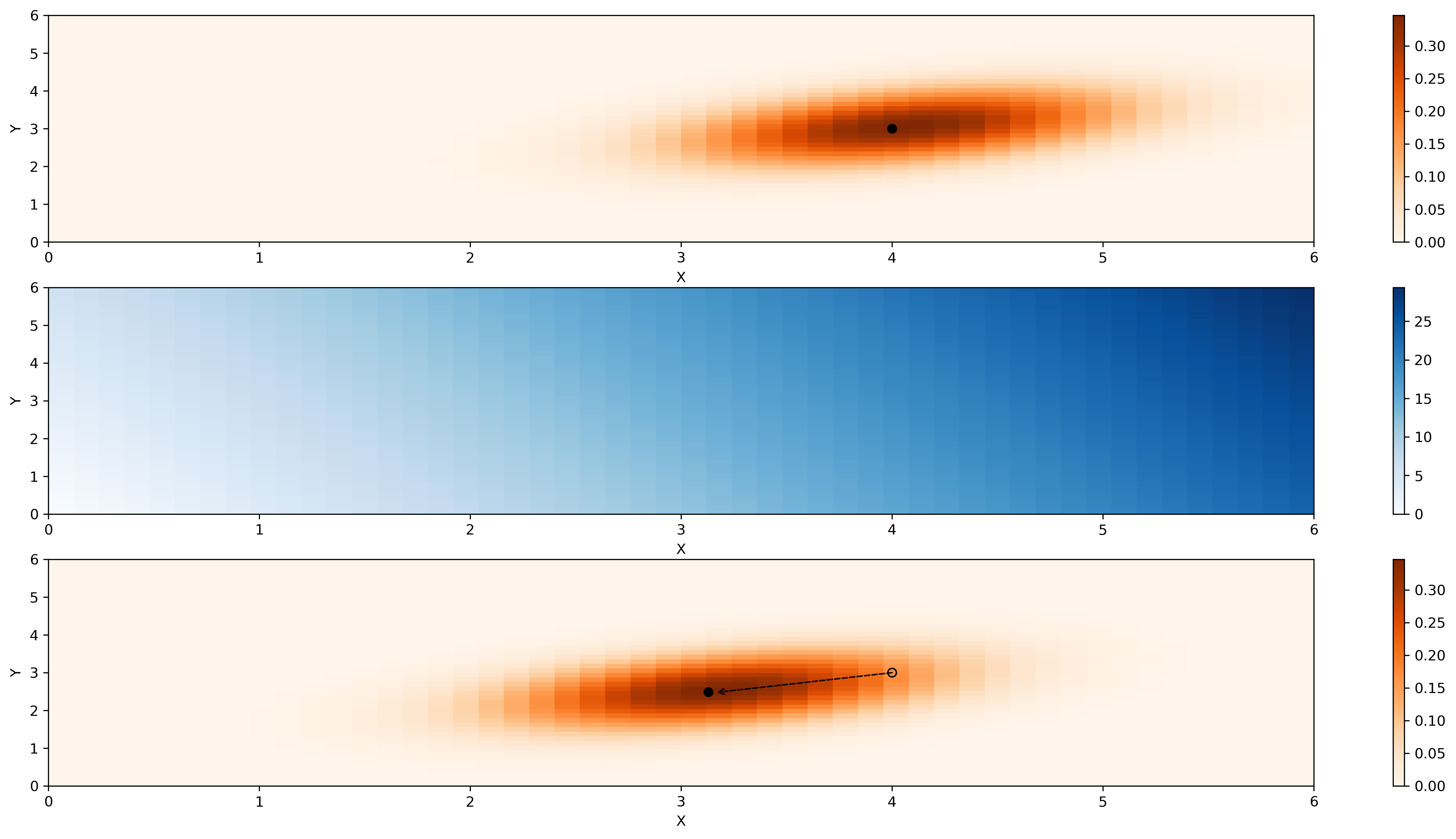
Figure 6: least favorable distribution for normally distributed data. First panel in red shows the density of $\mathcal{N}(\mu,\Sigma)$ $\mu=(4,3)^{T}$ $\Sigma=\begin{bmatrix}2&0.5\\ 0.5&2\end{bmatrix}$, the experimental distribution. The second panel shows $CATE=X^{T}\beta$, linear in X with $\beta=(4,1)^{T}$. The third panel shows the parameter shift of the least favorable distribution.

Here $\lambda_{0}=0.396$. $\mu^{*}=(3.1288,2.4852)$. The KL divergence, for two multivariate normal distributions $(\mu_{1},\Sigma_{1}),(\mu_{2},\Sigma_{2})$ is given by:
$KL(X_{1}||X_{2})=\frac{1}{2}\left[\log\left(\frac{|\Sigma_{2}|}{|\Sigma_{1}|}\right)-k+(\mu_{2}-\mu_{1})^{T}\Sigma_{2}^{-1}(\mu_{2}-\mu_{1})+tr(\Sigma_{2}^{-1}\Sigma_{1})\right]$. One could always compute the value of the KL divergence applying the nonparamteric formula $\delta^{*}=\int_{\mathcal{X}}\exp(-\lambda_{0}(\tau(X)-\tilde{\tau}))d\mu_{X}$ or in this case, the “parametric” formula given by the KL divergence between two normal distributions. In this example both ways of computing the correspond to $\delta^{*}=0.789$ corresponding to the mean shift illustrated above.

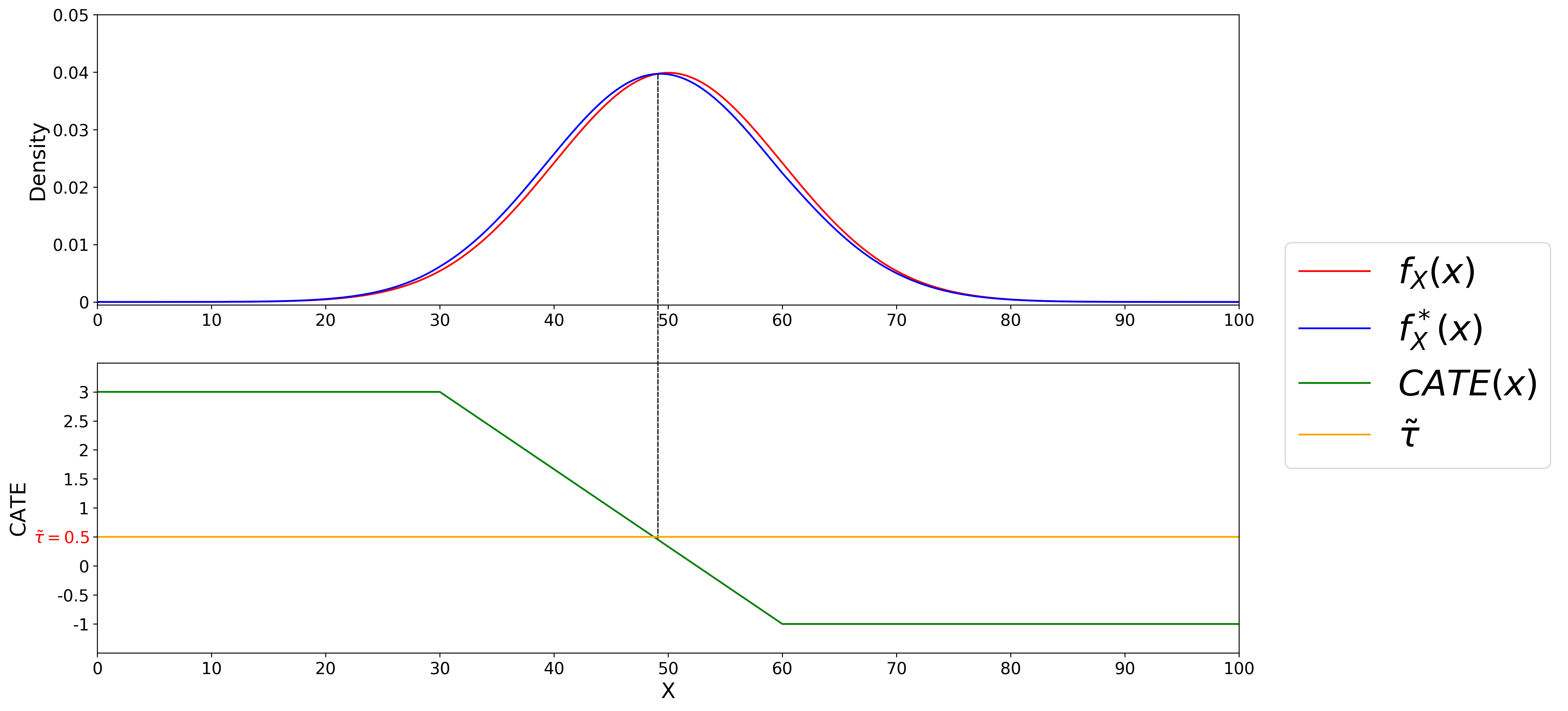
Figure 7: Piece-wise Linear CATE, experimental distribution is $\mathcal{N}(50,10^{2})$. Status quo ATE is 0.433, while $\tilde{\tau}=0.5$. Because the experimental ATE is lower than the least favorable , $F_{X}^{*}$ down-weights $F_{X}$ on the subset of $\mathbb{R}$ where the $\tau(x)$ is greater than $\tilde{\tau}$ and up-weights it where it’s lower. The blue curve is the closest curve to the red one, in KL-divergence, among the ones that satisfy $\tau\geq 0.5$.

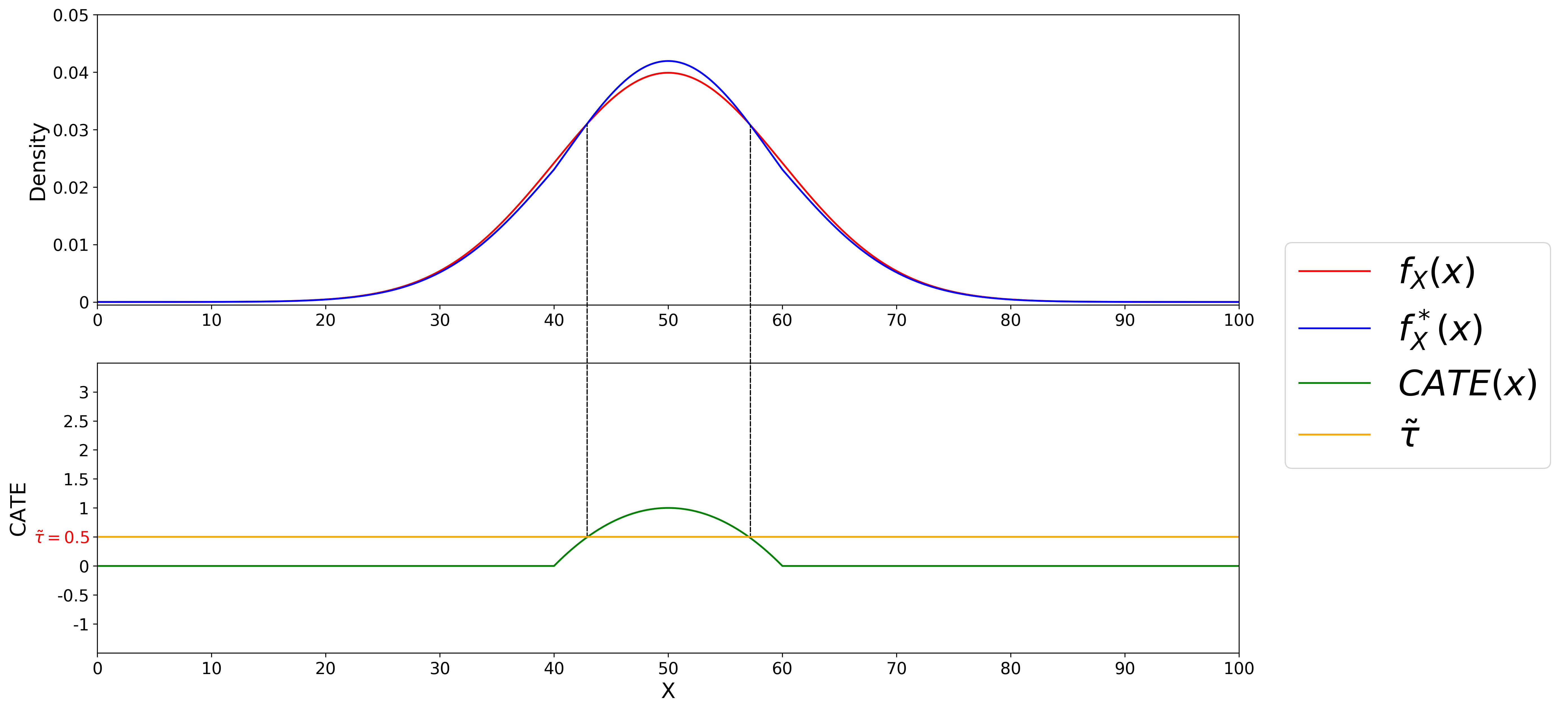
Figure 8: Piecewise Quadratic CATE, experimental distribution is $\mathcal{N}(50,10^{2})$. Status quo ATE is 0.484 while $\tilde{\tau}=0.5$. Because the experimental ATE is lower than the least favorable , $F_{X}^{*}$ down-weights $F_{X}$ on the subset of $\mathbb{R}$ where the $\tau(x)$ is smaller than $\tilde{\tau}$ and up-weights it where it’s greater. The blue curve is the closest curve to the red one, in KL-divergence, among the ones that satisfy $\tau\geq 0.5$.

Example 28.

Let’s now see graphically how to construct an example for a one dimensional continuous variable example. In Figures 7 and 8 conditional treatment effects, given the 1-dimensional variable $X$ are in green, the status quo distribution is $\mathcal{N}(50,10^{2})$ is in red. Suppose that the policy-maker’s wants to maintain the claim $ATE\leq 0.5$. The experimental ATE and the “least favorable” ATE are obtained by integrating the green curve $\tau(x)$ against the red curve $dF_{X}(x)$ (which has density $f_{X}(x)$) and the blue curve $dF^{*}_{X}(x)$ (which has density $f^{*}_{X}(x)$ respectively. The blue curve is the closest distribution to the status quo distribution in red, as measured by the KL divergence, that delivers the “least favorable ” ATE $\tilde{\tau}=0.5$.

References

- Altonji et al. [2005] J. G. Altonji, T. E. Elder, and C. R. Taber. Selection on observed and unobserved variables: Assessing the effectiveness of catholic schools. Journal of political economy, 113(1):151–184, 2005.
- Andrews et al. [2017] I. Andrews, M. Gentzkow, and J. M. Shapiro. Measuring the sensitivity of parameter estimates to estimation moments. The Quarterly Journal of Economics, 132(4):1553–1592, 2017.
- Antoine and Dovonon [2020] B. Antoine and P. Dovonon. Robust estimation with exponentially tilted hellinger distance. Journal of Econometrics, 2020.
- Armstrong and Kolesár [2021] T. B. Armstrong and M. Kolesár. Sensitivity analysis using approximate moment condition models. Quantitative Economics, 12(1):77–108, 2021.
- Athey et al. [2016] S. Athey, G. W. Imbens, and S. Wager. Approximate residual balancing: De-biased inference of average treatment effects in high dimensions. arXiv preprint arXiv:1604.07125, 2016.
- Bonhomme and Weidner [2018] S. Bonhomme and M. Weidner. Minimizing sensitivity to model misspecification. arXiv preprint arXiv:1807.02161, 2018.
- Broderick et al. [2020] T. Broderick, R. Giordano, and R. Meager. An automatic finite-sample robustness metric: Can dropping a little data change conclusions? arXiv preprint arXiv:2011.14999, 2020.
- Cartwright and Hardie [2012] N. Cartwright and J. Hardie. Evidence-based policy: A practical guide to doing it better. Oxford University Press, 2012.
- Chernozhukov et al. [2013] V. Chernozhukov, S. Lee, and A. M. Rosen. Intersection bounds: estimation and inference. Econometrica, 81(2):667–737, 2013.
- Chernozhukov et al. [2018] V. Chernozhukov, D. Chetverikov, M. Demirer, E. Duflo, C. Hansen, W. Newey, and J. Robins. Double/debiased machine learning for treatment and structural parameters. Econometrics Journal, 21(1):C1–C68, 2018.
- Chernozhukov et al. [2020] V. Chernozhukov, J. C. Escanciano, H. Ichimura, W. K. Newey, and J. M. Robins. Locally robust semiparametric estimation, 2020.
- Christensen and Connault [2019] T. Christensen and B. Connault. Counterfactual sensitivity and robustness. arXiv preprint arXiv:1904.00989, 2019.
- Cinelli and Hazlett [2020] C. Cinelli and C. Hazlett. Making sense of sensitivity: Extending omitted variable bias. Journal of the Royal Statistical Society: Series B (Statistical Methodology), 82(1):39–67, 2020.
- Deaton [2010] A. Deaton. Instruments, randomization, and learning about development. Journal of economic literature, 48(2):424–55, 2010.
- Donsker and Varadhan [1975] M. D. Donsker and S. S. Varadhan. Asymptotic evaluation of certain markov process expectations for large time, i. Communications on Pure and Applied Mathematics, 28(1):1–47, 1975.
- Finkelstein [2013] A. Finkelstein. Oregon health insurance experiment public use data, 2013.
- Finkelstein et al. [2012] A. Finkelstein, S. Taubman, B. Wright, M. Bernstein, J. Gruber, J. P. Newhouse, H. Allen, K. Baicker, and O. H. S. Group. The oregon health insurance experiment: evidence from the first year. The Quarterly journal of economics, 127(3):1057–1106, 2012.
- Gechter [2015] M. Gechter. Generalizing the results from social experiments: Theory and evidence from mexico and india. manuscript, Pennsylvania State University, 2015.
- Hartman [2020] E. Hartman. Generalizing experimental results. In J. Druckman and D. Green, editors, Advances in Experimental Political Science. Cambridge University Press, 2020.
- Ho [2020] P. Ho. Global robust bayesian analysis in large models. 2020.
- Horowitz and Manski [1995] J. L. Horowitz and C. F. Manski. Identification and robustness with contaminated and corrupted data. Econometrica: Journal of the Econometric Society, pages 281–302, 1995.
- Hsu et al. [2020] Y.-C. Hsu, T.-C. Lai, and R. P. Lieli. Counterfactual treatment effects: Estimation and inference. Journal of Business & Economic Statistics, pages 1–16, 2020.
- Huber [1965] P. J. Huber. A robust version of the probability ratio test. The Annals of Mathematical Statistics, pages 1753–1758, 1965.
- Imbens and Rubin [2015] G. W. Imbens and D. B. Rubin. Causal inference in statistics, social, and biomedical sciences. Cambridge University Press, 2015.
- Jeong and Namkoong [2020] S. Jeong and H. Namkoong. Robust causal inference under covariate shift via worst-case subpopulation treatment effects. In Conference on Learning Theory, pages 2079–2084. PMLR, 2020.
- Kennedy et al. [2020] E. H. Kennedy, S. Balakrishnan, M. G’Sell, et al. Sharp instruments for classifying compliers and generalizing causal effects. Annals of Statistics, 48(4):2008–2030, 2020.
- Kowalski [2018] A. E. Kowalski. Reconciling seemingly contradictory results from the oregon health insurance experiment and the massachusetts health reform. Technical report, National Bureau of Economic Research, 2018.
- Luenberger [1997] D. G. Luenberger. Optimization by vector space methods. John Wiley & Sons, 1997.
- Masten and Poirier [2020] M. A. Masten and A. Poirier. Inference on breakdown frontiers. Quantitative Economics, 11(1):41–111, 2020.
- Meager [2019] R. Meager. Understanding the average impact of microcredit expansions: A bayesian hierarchical analysis of seven randomized experiments. American Economic Journal: Applied Economics, 11(1):57–91, 2019.
- Newey and McFadden [1994] W. K. Newey and D. McFadden. Chapter 36 large sample estimation and hypothesis testing. volume 4 of handbook of econometrics, 1994.
- Oster [2019] E. Oster. Unobservable selection and coefficient stability: Theory and evidence. Journal of Business & Economic Statistics, 37(2):187–204, 2019.
- Posner [1975] E. Posner. Random coding strategies for minimum entropy. IEEE Transactions on Information Theory, 21(4):388–391, 1975.
- Rosenbaum and Rubin [1984] P. R. Rosenbaum and D. B. Rubin. Reducing bias in observational studies using subclassification on the propensity score. Journal of the American statistical Association, 79(387):516–524, 1984.
- Tukey [1960] J. W. Tukey. A survey of sampling from contaminated distributions. Contributions to probability and statistics, pages 448–485, 1960.
- Van der Vaart [2000] A. W. Van der Vaart. Asymptotic statistics, volume 3. Cambridge university press, 2000.
- Williams [2020] M. J. Williams. External validity and policy adaptation: From impact evaluation to policy design. The World Bank Research Observer, 35(2):158–191, 2020.