Generator coordinate method for transition-state dynamics in nuclear fission

Abstract

Since its beginnings, fission theory has asumed that low-energy induced fission takes place through transition-state channels at the barrier tops. Neverthess, up to now there is no microscopic theory applicable to those conditions. We suggest that modern reaction theory is suitable for this purpose, and propose a methodology based on a configuration-interaction framework using the Generator Coordinate Method (GCM). Simple reaction-theoretic models are constructed with the Gaussian Overlap Approximation (GOA) to parameterize both the dynamics within the channels and their incoherent couplings to states outside the barrier. The physical characteristics of the channels examined here are their effective bandwidths and the quality of the coupling to compound-nucleus states as measured by the transmission factor $T$. We also investigate the spacing of GCM states with respect to their degree of overlap. We find that a rather coarse mesh provides an acceptable accuracy for estimating the bandwidths and transmission factors. The common numerical stability problem in using the GCM is avoided due to the choice of meshes and the finite bandwidths of the channels. The bandwidths of the channels are largely controlled by the zero-point energy with respect to the collective coordinate in the GCM configurations.

I Introduction

An important goal in the description of fission reactions is to understand their excitation functions, that is, the probability that the reaction leads to fission as a function of the total energy. Another important goal is to understand the properties of the daughter nuclei after a fission event. There has been enormous progress in recent years on understanding the characteristics of the final state thanks to improved computational tools in many-body quantum mechanics such as the time-dependent Hartree-Fock-Bogoliubov approximation whitepaper ; bulgac2016 .

The theory of the excitation function in reactions with many possible outcomes has not seen comparable advances. Fission theory has relied on the transition-state hypothesis since the original paper by Bohr and Wheeler in 1939 bo39 and continuing up to the present era bo13 ; capote2009 ; chadwick2006 ; chadwick2011 ; cap2011 ; lu2016 ; schmidt1991 . Briefly, it is encapsulated in the formula for the decay rate $\Gamma_{\rm BW}$

$$\Gamma_{\rm BW}=\frac{1}{2\pi\rho}\sum_{\mu}T_{\mu}$$ (1)

where $\mu$ labels channels, $\rho$ is the level density of the compound nucleus, and $T_{\mu}$ is a transmission coefficient or conductance. It is also identical to the penetration factor in subbarrier conductance. It satisfies the bounds

$$0\leq T_{\mu}\leq 1.$$ (2)

Typically the energy dependence of $T$ is assumed to be the same as that of a particle traversing a one-dimensional potentiala barrier, but that is a pure guess absent a microscopic understanding of the many-body Hamiltonian dynamics.

It is clear that the present time-dependent formulations are ill-suited to the task of describing the barrier-crossing dynamics in heavy nuclei. We expect that a formulation using reaction theory might be more successful. In this paper, we examine how the transition-state dynamics might be realized in a reaction theory based on a configuration-interaction treatment of the Hamiltonian.

In the theory of large nuclei, one starts with the wave functions of self-consistent mean-field theory, such as those given by the energy density functionals of Skyrme, Gogny, or relativistic formulations bender03 . Besides the self-consistent solutions of the Hartree-Fock (HF) or Hartree-Fock-Bogoliubov (HFB) equations, an adequate basis of states for studying transport properties can be constructed using the Generator Coordinate Method (GCM). This requires the calculation of mean-field configurations that are constrained by one or more single-particle fields. The GCM has been used previously for modeling fission dynamics near the barrier top go05 ; re16 ; ta17 . In those works, the authors used GCM with two constraining fields and the Gaussian Overlap Approximation (GOA) to map the Hamiltonian onto a two-dimensional Schrödinger equation. However, the steps needed to arrive at a Schrödinger equation ignore the statistical aspects of the decay and gives no hint of a connection to Eq. (1). Here we only need the matrix elements between GCM configurations in our reaction-theoretic approach, avoiding the mapping onto a Schödinger equation.

In an earlier paper be21 we showed how one can derive the transition-state formula in a highly simplified configuration-interaction approach. Here we shall use the same reaction theory formalism to calculate transmission coefficients, but with a more realistic description of the channels. An important advantage of the reaction theory is that statistical aspects of the theory can be easily included in the formalism ha21 .

A technical obstacle in the GCM approach is the nonorthogonality of the basis configurations. As will be shown, its formal difficulties are avoided by making use of the many-body Green’s function defined in Eq. (4) below. A related problem is the danger of numerical instabilities when overlaps between configurations are large. We will show that this problem does not arise because one can use coarse bases without much loss of accuracy.

For investigating transition channels in fermionic systems, the general characteristics can be derived independently of the details of the constraining field. A configuration is labeled by the expectation value of the field; we shall call the expectation value $q_{k}$ for a $k$-th configuration in a finite-dimensional basis.

Besides the internal properties of the channel, one needs specific information about the coupling to the reservoirs of states on either side of the channel. The situation is very similar to the cables in computer networks. The cable has a characteristic impedance, and conductance between the connected devices depends on impedance matching. An optimally matched coupling yields a transition conductance $T=1$. Mismatches decrease it and makes it dependent on the signal frequency. For the fission theory, one needs to understand in detail the interaction connecting compound-nuclear states to the states in the channel. That is beyond the scale of this paper; we will treat these couplings schematically.

II GCM methodology for transmission channels

The usual procedure for applying the GCM to nuclear spectroscopy consists of the following steps.

1) Select a set of configurations calculated in mean-field theory and constrained by some physical one-body field such as the mass quadrupole moment $Q$. The set of expectation values of the field $(q_{1},q_{2},...q_{N})$ defines an $N$-dimensional basis for the configuration space. In more advanced approaches the configurations are projected to restore broken symmetries.

2) Calculate the matrix $\boldsymbol{N}$ of overlaps between configurations and the matrix $\boldsymbol{H}$ of the Hamiltonian or the energy functional that plays the role of the Hamiltonian in the mean-field theory. Here and below we use boldface symbols for matrices.

3) Solve the hermitian eigenvalue problem (i.e., the Hill-Wheeler equation)

$$\boldsymbol{H}\psi=E\boldsymbol{N}\psi$$ (3)

for energies $E$ and corresponding $N$-dimensional wave functions $\psi$.

4) Check for convergence by varying the number of configurations $N$ in the calculation. The effect on the properties in the low-energy part of the spectrum should be small.

Steps 1) and 2) are the same for calculating reaction rates in the GCM, but the remaining steps are completely different. Namely, the new steps are:

3’.) In a new step 3), the Hamiltonian is made complex by adding imaginary terms $-\boldsymbol{\Gamma}_{j}/2$ to it and calculate the Green’s function. This replaces the matrix diagonalization in the old step 3). Each $\boldsymbol{\Gamma}_{j}$ is a matrix of decay rates to states $j$ outside of the model space. It is a sum of rank-one matrices, each corresponding to an $S$-matrix channel ka15 . See Eq. (8) below for a consistent implementation in our modeling framework. Time-dependent methods also make use of complex Hamiltonians to treat fluxes out of the model spaces, as for in Ref. re16 , but there the $\boldsymbol{\Gamma}_{j}$ can be parameterized as diagonal matrices. There are two decay modes in the present fission study, one corresponding to the set of compound nucleus states and the other to states in the second well and beyond. We label $a$ and $b$, respectively, in the equation below. The required Green’s function is

$$\boldsymbol{G}(E)=(\boldsymbol{H}-i\boldsymbol{\Gamma}_{a}/2-i\boldsymbol{\Gamma}_{b}/2-\boldsymbol{N}E)^{-1}.$$ (4)

5.) The transmission factor $T_{ab}$ between reservoir $a$ and $b$ is given by $S$-matrix expression.

$$T_{ab}=\sum_{\mu\in a}\sum_{\nu\in b}|S_{\mu\nu}|^{2}.$$ (5)

The $S$-matrix is usually written in terms of $\boldsymbol{H}$ and a set of reduced decay amplitudes as in (ka15, , Eq. 14-19). In our application the phase information in $S_{\mu\nu}$ is not needed and we use the Datta formula da95 ; al21 to calculate $T_{ab}$ in terms of $\boldsymbol{G}$ and $\boldsymbol{\Gamma}$,

$$T_{ab}=\sum_{jklm}(\boldsymbol{\Gamma}_{a})_{jk}\boldsymbol{G}_{kl}(\boldsymbol{\Gamma}_{b})_{lm}\boldsymbol{G}^{*}_{mim}={\rm Tr}\,\left(\boldsymbol{\Gamma}_{a}\boldsymbol{G}\boldsymbol{\Gamma}_{b}\boldsymbol{G}^{*}\right).$$ (6)

The resulting $T_{ab}$ is a continuous real function of $E$; the individual channels satisfy $0\leq T_{\mu\nu}\leq 1$. As in the procedure for spectroscopic studies, one gains confidence by varying the dimension of the configuration spaces.

III Decay widths

What is left now are the tasks of constructing the matrices $\boldsymbol{N}$, $\boldsymbol{H}$ and $\boldsymbol{G}$. The overlap matrix $\boldsymbol{N}$ is simply the determinant of the orbital overlaps when the configurations are pure Slater determinants. We shall not go into the well-known difficulties la09 in defining $\boldsymbol{H}$ when the energetics are based on an energy functional rather than a Hamiltonian, and simply remark that the prescriptions for dealing with an energy density functional are well established.

A new issue arises in defining the decay matrix. Our guiding principle is Fermi’s Golden Rule for the decay of a configuration $j$ into a set of states $a$. This reads

$$\Gamma_{a,j}=2\pi\sum_{k\in a}|\langle k|v|j\rangle|^{2}\delta(E_{k}-E),$$ (7)

where the density-of-states function $\sum_{k\in a}\delta(E_{k}-E)$ smeared out in some way for numerical computations. The state $j$ is in the set of configurations defining the transition-state, while the set $a$ are configurations in the compound nucleus on one side or the post-barrier configurations on the other side. The interaction connect the transition-state configurations to the rest is denoted $v$.

Due to the lack of orthogonality among the states in $\boldsymbol{H}$ an individual decay channel may couple to more than one configuration in the transition-state channel. This implies that $\boldsymbol{\Gamma}$ can have off-diagonal matrix elements. If these off-diagonal matrix elements are ignored, the individual transmission factors may violate the Eq. (2).

The matrix structure can be achieved in a generalized Fermi Golden Rule of the form

$$(\boldsymbol{\Gamma}_{j})_{kk^{\prime}}=2\pi\sum_{j\in a}\langle k|v|j\rangle\langle k^{\prime}|v|j\rangle\delta(E_{j}-E).$$ (8)

In this work we do not attempt to compute the $\boldsymbol{\Gamma}$ from Eq. (8) from the Hamiltonian but simply assume the separable approximation

$$(\boldsymbol{\Gamma}_{j})_{kk^{\prime}}=\gamma_{j}g_{j}(k)g_{j}(k^{\prime}).$$ (9)

to parameterize it.

IV Examples of GOA Hamiltonians

In these examples the transition-state channel is composed of one or two chains of configurations with varying assumptions about the Hamiltonian $\boldsymbol{H}$. Calling the collective GCM coordinate $q$, we take chains of $N$ regularly spaced states spanning an interval $[q_{1},q_{N}]$ with a mesh spacing $\Delta q=(q_{N}-q_{1})/(N-1)=1$. To examine the dependence on the mesh spacing the calculations are carried out for two choices of mesh spacing, keep the Hamiltonian and the total length $Q_{T}=(N-1)\Delta q=3$ fixed.

To derive the matrix elements in the model, we assume that the variables in the wave function of a configuration $\Psi_{q_{k}}$ can be decomposed into a continuous coordinate $q$ and a set of other coordinates $\xi$, and the dependence on $q$ is Gaussian in the GCM configuration,

$$\Psi_{q_{k}}(\xi,q)=\Psi^{\prime}(\xi)(\pi s^{2})^{-1/4}\,e^{-(q-q_{k})^{2}/(2s^{2})}.$$ (10)

Here $s$ is the width of the Gaussian wave packet. Then the overlap matrix has elements

$$\boldsymbol{N}_{jk}=\exp\left(-(q_{j}-q_{k})^{2}/4s^{2}\right).$$ (11)

The model Hamiltonian matrix is constructed with separate kinetic and potential energy terms,

$$\boldsymbol{H}=\boldsymbol{K}+\boldsymbol{V}.$$ (12)

For the matrix $\boldsymbol{K}$, we are guided by the GCM theory for a cluster of particles bound together by a translationally invariant particle-particle interaction, but free of any external forces be19c . Here the collective variable is $x$, the position of the center of mass of the cluster. Under the factorization hypothesis (Eq. (10) the GCM Hamiltonion matrix element is

$$\boldsymbol{K}_{jk}=E_{K}(1-(q_{j}-q_{k})^{2}/2s^{2})\boldsymbol{N}_{jkj}.$$ (13)

with $E_{K}$ given by

$$E_{K}=\frac{\hbar^{2}}{2Ms^{2}}$$ (14)

and $M$ denoting the mass of the particles be19c . We will treat a possible potential energy $V(q)$ in a similar way in Section B below.

We make the same separable approximation for the for imaginary matrices $\boldsymbol{\Gamma}$, centering their wave packets at the endpoints of the chain. The resulting parameterization from Eq. (9) has the separable function

$$g_{j}(k)=\boldsymbol{N}_{kj}$$ (15)

and $\gamma$ as an arbitrary real parameter. Here we assume $\gamma_{1}=\gamma_{N}\equiv\gamma$.

The resulting Green’s function to be evaluated is the inverse of the matrix

$$\boldsymbol{H}_{jk}-i\gamma\boldsymbol{N}_{j1}\boldsymbol{N}_{k1}/2-i\gamma\boldsymbol{N}_{jN}\boldsymbol{N}_{kN}/2-\boldsymbol{N}_{jk}E.$$ (16)

In summary, aside from the term $\boldsymbol{V}$, the model presented here has three dimensionless parameters: $N$, the number states in channel; $\Delta q/s$, the spacing of the states in units of the width of the collective wave packet; and $\gamma/E_{K}$, the strength of the imaginary decay width in units of the zero-point kinetic energy. The energy scale is set by $E_{K}$. The width of the Gaussian packet $s$ is also dimensionful and sets the scale for the overlap distance between configurations bo90 .

IV.1 A single flat channel

The first model we investigate is a flat chain composed of $N=4$ configurations with overlaps between them set to $\Delta q/s=\sqrt{5}$. This choice was shown in Ref. be19c to give a good compromise between accuracy and computational effort. The channel is depicted as “A” in Fig. 1. The states indicated by black circles are the ones included in the $N=4$ model. We will also examine the same model with 7 states; the added states are shown as the red circles. For the 7-state model $\Delta q$ is reduced by a factor of 2 while $s$ remains fixed.

Figure 1: Relationship between states in the models described in Sections IV.A,B, and C. The states in the 4-state and 7-state channels are shown as black and black+red circles respectively. The real part of the Hamiltonian couples the states in the channel or channels; the couplings to the reservoirs are parameterized by the imaginary part of the Hamiltonian.

The diagonal energies of the GCM states $E_{K}$ are taken to be $E_{K}=5/4$ and the strengths of the absorption at the ends are $\gamma=1$. With these parameters the overlap between neighboring states is fairly small, $\boldsymbol{N}_{k,k+1}=0.28$. The resulting transmission factor $T(E)$ calculated by Eq. (6) is shown in Fig. 2 as the black solid line.

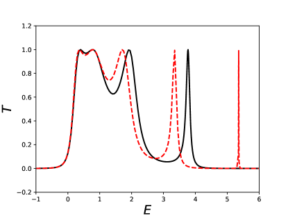
Figure 2: Transmission factor for a chain of length $Q_{T}=3\sqrt{5}$ comparing GCM calculations for 4 and 7 states in the chain (solid black and dashed red lines, respectively). Besides the peaks visible in the figure, there are 2 extremely narrow peaks at somewhat higher energy in the 7-state model. The parameters of the Hamiltonian are $(s,E_{0},\gamma)=(1/\sqrt{5},5/4,1)$. See the Supplementary Material for the computer scripts used to calculate the data presented here and later in the Figures.

One sees a structure of 4 peaks, each close to an eigenvalue of the Hill-Wheeler Eq. (3). Physically, the peaked structure arises from the wave reflection at the ends of the channel. Note that the range of $T(E)$ satisfies $0\leq T\leq 1$ as required by the unitarity of the $S$ matrix. Note also that the channel starts conducting near $E\approx 0$, as would be the case for a classical channel governed by a Hamiltonian without any zero-point energy. The adequacy of the mesh spacing can be assessed by shrinking it. Decreasing it by a factor of 2, the same interval contains 7 seven states instead of 4. The resulting transmission factor is shown as the dashed red line in Fig. 2. One sees that in the low-energy region it is quite similar to the 4-state approximation. However, it has 3 additional peaks at higher energy, corresponding to the high-energy eigenfunctions of the 7-d model. These peaks are much narrower than the lower ones and can be neglected in calculating integrated transmission rates. The same behavior would continue with finer mesh spacings; there would remain 4 peaks in the energy region $[0,2]$ and the additional narrow peaks would appear at higher and higher energies. The qualitative aspects of this behavior can be easily understood. With a finite mesh spacing of Gaussian wave packets one can approximate plane wave with a good fidelity for low momentum, but there is a momentum cutoff controlled by the mesh spacing. In the transmission channel as parameterized, the momentum at the injection and exit point is controlled by the Gaussian width parameter $s$. The momentum match to the channel parameters suppresses the transmission to the high-momentum modes in the channel. We conclude that fairly sparse meshes are adequate for representing the overall conductivity of flat transmission channels.

As mentioned earlier, very fine mesh spacings often lead to numerical instabilities in the spectroscopic applications of the GCM. The usual fix is to make a singular value decomposition of the overlap matrix, throwing out eigenfunctions that have small norms. It is instructive to see what happens when the same procedure is applied here.

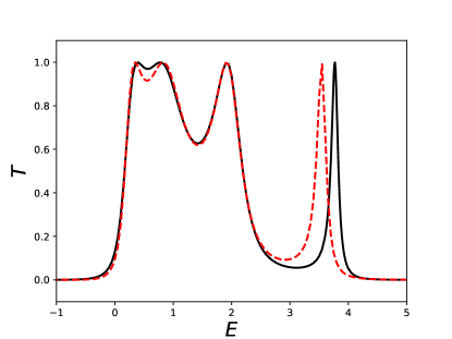
Figure 3: Transmission factor for a chain of length $q=4$ comparing GCM calculations for 4 and 7 states in the chain (solid black and dashed red lines, respectively). The difference with Fig. 2 is that the 7-d space was truncated to 4 dimensions by the singular value decomposition of the overlap matrix. The Hamiltonians are the same as in Fig. 2.

Fig. 3 compares the $4$-state model with the 7-state model truncated to 4 states. That is, we diagonalize the norm matrix in the 7-state model and project the Hamiltonian on the basis of the 4 eigenfunctions having the highest eigenvalues of the norm matrix. One sees that the resonance positions are rather close and the widths are also very similar. There is no obvious benefit from starting out with a larger space. Since there is no need to truncate the space for reasons of numerical stability, this aspect of the usual methodology can be dropped.

We next examine how $T(E)$ depends on the strength of the absorption at the ends of the channel. Fig. 4 shows $T(E)$ for a range of absorption strengths $\gamma$.

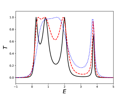
Figure 4: Transmission factors in the 4-d model for several values of absorption strength: $\gamma=0.5$ (solid black line); $\gamma=1.0$ (red dashed line); $\gamma=2.0$ (blue dotted line). All peak tops are at $T=1$, but may not be visible in the figure due the finite grid of energies.

Obviously, for small $\gamma$ the channel acts as a resonant cavity with sharply defined resonances and the overall conductance is low. For the larger $\gamma$’s the reflection amplitude is small and the individual peak broaden and merge together.

IV.2 A parabolic channel

In this section we extend the model to include a potential barrier. We take the shape of the barrier as an inverted parabola, as is often assumed in phenomenological treatments.

Under the factorization Ansatz Eq. (10) the GCM matrix elements of a potential depending only on the $q$ coordinate are given by

$$\boldsymbol{V}_{jk}=$$

$$\frac{1}{s\pi^{1/2}}\int^{\infty}_{-\infty}dq\,V(q)e^{-(q-q_{j})^{2}/2s^{2}-(q-q_{k})^{2}/2s^{2}}.$$ (17)

The $V(q)$ is taken as the parabolic form

$$V(q)=V_{2}(q-q_{b})^{2}$$ (18)

where $q_{b}$ is at the center of the barrier. The resulting GCM matrix elements are

$$\boldsymbol{V}_{jk}=V_{2}\left[\left(\frac{q_{j}+q_{k}}{2}-q_{b}\right)^{2}+\frac{s^{2}}{2}\right]\boldsymbol{N}_{jk}.$$ (19)

The matrix $\boldsymbol{V}$ of these elements are added to the Hamiltonian defined in Eq. (12) and (13). Note that the diagonal potential matrix elements are slightly below the defining potential due to the second term in Eq. (19). The diagonal energies are indicated in the channel marked “B” in Fig. 1. For a numerical example we take $V_{2}=-1/2$. The channel Hamiltonian has 4 eigenenergies ranging from $-$0.4 to 3.3. Fig. 5 shows the transmission factor as a function of energy taking $\gamma=1.0$.

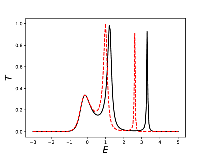
Figure 5: Transmission factor in the 4-d and 7-d models with a parabolic barrier. Solid black line: 4x4 model; red dashed line: 7x7 model. As in the previous figures, the narrow peaks extend up to $T=1$ in height.

Three peaks are visible. In terms of the channel eigenstates, the two lowest are responsible for the broad peak at $E\approx 0$. It appears that the barrier suppresses the maximum conductance since the peak height much less than one. At higher energies the $T$ can approach maximum value of one, but the coupling is weaker and the peaks are narrower.

We believe this behavior is generic for channels that follow the topography of the potential energy surface. This is the case when they are constructed using an adiabatic approximation. To see that the results are not an artifact of the GCM mesh spacing, we also show the transmission factor taking a finer mesh with 7 GCM configurations instead of 4. One sees that the low-energy conductance is almost the same. At higher energies, the narrowing of the peaks is also similar, although the peaks are somewhat shifted in energy.

IV.3 Two crossing channels

To understand better the adiabatic approximation, we consider a model in which the adiabatic channels arise from coupling between diabatic ones. We start with two diabatic channels that cross as depicted in graph “C” in Fig. 1. The dashed black lines link configurations that have large matrix elements in HF mean field theory; resulting chains are the diabatic paths in the dynamics. Adiabatic dynamics arise when one first diagonalizes the Hamiltonian within the subspace at fixed $q_{k}$. These are indicated by the curved red dotted lines in the Figure. The picture of adiabatic channels peaking at the barrier top is unavoidable in transition-state theory as implemented in Eq. (1).

For the Hamiltonian model we add linear potentials to generate the diabatic paths together with a constant interaction between configurations states at the same positions $q_{k}$. The matrix elements for a potential having a constant slope $V_{a}(q)=v_{a}q$ are given by

$$\boldsymbol{V}_{aj;ak}=v_{a}\left(\frac{q_{j}+q_{k}}{2}-q_{b}\right)\boldsymbol{N}_{jk}\delta_{aa^{\prime}}.$$ (20)

The label $a$ applies to the upward-sloping diabatic channel; the downward-sloping one will be label $b$. The other term to be added to the Hamiltonian is the coupling $h_{c}$ between the configurations of the two diabatic channels. We take the coupling as a constant independent of $q_{k}$. Again invoking factorization hypothesis, the nonzero matrix elements are

$$\boldsymbol{H}_{aj,bk}=h_{c}N_{jk}.$$ (21)

For the numerical example, we take $v_{a}=0.5$, $v_{b}=-0.5$ and $h_{c}=0.8$.

As depicted in Fig. 1 there are now 4 decay matrices to be added to the Hamiltonian. We assume that all final states are orthogonal to each other, so we can apply the transmission formula Eq. (6) with an incoherent sum over all four combinations $(a1,b1)\rightarrow(aN,bN)$.

In the adiabatic approximation only the transmission factor from the two lowest states at the ends are included,

$$T_{\rm adiabatic}\approx T_{a1,bN}.$$ (22)

It is shown as the red dashed line in Fig. 6. The dotted blue line shows the combined transmission factor that includes including the upper adiabatic channel as well,

$$T^{\prime}_{\rm adiabatic}\approx T_{a1,bN}+T_{b1,aN}.$$ (23)

These are to be compared to the full transmission factor (solid black line) including all contributions,

$$T=T_{a1,bN}+T_{a1,aN}+T_{b1,aN}+T_{b1,bN}.$$ (24)

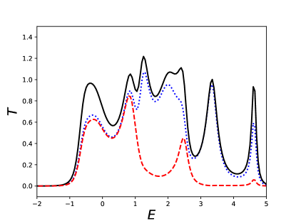
Figure 6: Transmission factor for the Hamiltonian “C₈” depicted in Fig. 1. Solid black line: all contributions to $T$; red line: lowest adiabatic contribution; blue line: both adiabatic contributions. Note that the total transmission coefficient can be larger than one in the cases where two channels contribute.

One sees that the adiabatic approximation works well overall when both channels are included. The second channel adds hardly anything in the region where the lower channel is open, but fills out the higher region $1.0<E<2.5$. Another interesting finding, not very visible in the figure, is that the adiabatic approximation significantly underpredicts the transmission factor at the lowest energies. This inadequacy of the approximation was noted earlier in Refs. ha20 ; gi14 .

We have also calculated $T$ without any coupling between the diabatic channels. As expected, that treatment seriously underpredicts the transmission coefficient.

V General conclusions

.

A few tentative conclusions may be drawn from the simple models presented here. First of all, one does not need fine collective-coordinate meshes in the GCM configuration space. A mesh spacing giving overlaps of 0.3 between a configuration and its diabatic neighbor seems adequate; smaller mesh spacings will produce narrow resonances at high energy, but the coarse properties of the channel will remain the same. The second conclusion is that momentum matching is an important consideration in the channel coupling to the reservoir states. It produces an effective energy cutoff in the conductance of the channel. The energy scale for this effect is given by the zero-point energy of the collective coordinate in the mean-field wave function. To give a sense of that, we present in Table I some characteristics of the transmission function $T(E)$ for the models discussed in the previous section. The first characteristic is the integrated transmission factor. This is reported in the Table in units of $E_{K}$,

$$I_{T}=\int_{-\infty}^{\infty}dE\,T(E)/E_{K}.$$ (25)

Comparing the 4-state models with the 7-state models A and B, one sees less than a 10% change in the integrated transmission.

A second finding is that the transmission is strong only in a limited energy interval. To examine this point in a quantitative way, we have computed the $T$-weighted average energy

$$\langle E\rangle=\left.\int dE\,E\,T(E)\right/\int dE\,T(E)$$ (26)

and its standard deviation, $\sigma(E)=\langle E^{2}\rangle-\langle E\rangle^{2}$. These quantities are shown in the last two columns of the table.

Model	$I_{T}$	$\langle E\rangle/E_{K}$	$\sigma(E/E_{K})$
A4	1.69	1.17	0.81
A7	1.65	1.11	0.77
B4	0.61	0.80	0.84
B7	0.56	0.60	0.67
C8	3.12	1.28	1.15
C${}^{a}_{8}$	2.54	1.31	1.09

Table 1: Integrated channel properties of the models discussed in the text. The model labels refer to the subsection in Sect. IV where they were discussed. The subscript refers to the dimension of the GCM space. The average energy $\langle E\rangle$ is computed with respect to the Hamiltonian at the midpoint of the $q$ interval omitting the zero-point energy $E_{K}$. In case C, the energy is the adiabatic one computed by diagonalizing the 2x2 matrix mixing the two GCM states. The row marked C${}^{a}_{8}$ ignores the coupling between the adiabatic channels.

Both quantities exhibited in the Table support our conclusion that one can safely use coarse meshes to define the channels. The averages change by 25% or less in comparing the 4-state and 7-state models. The average energy is comparable to the zero-point energy in the flat channel. In the parabolic channel the average energy is somewhat lower due barrier effect; in this case the finer mesh has a significant affect. However, it may be seen from the $\sigma(E/EK)$ column that the spread of energies is about the same.

Model $C_{8}$ simulating adiabatic transmission by two interacting diabatic channels has about twice the integrated transmission strength as model A, which is hardly surprising. Note however that the coupling between the two diabatic channels is significant: model $C^{a}_{8}$ ignores the coupling and its $I_{T}$ is smaller by 20%. In present fission theory such couplings are neglected, and this finding confirms that approximation in phenomological models.

References

- (1) M. Bender et al., J. of Phys. G47, 113002 (2020).
- (2) A. Bulgac, P. Magierski, K.J. Roche, and I. Stetcu, Phys. Rev. Lett. 116, 122504 (2016).
- (3) N. Bohr and J.A. Wheeler, Phys. Rev. 56, 426 (1939).
- (4) O. Bouland, J.E. Lynn, and P. Talou, Phys. Rev. C 88 054612 (2013).
- (5) R. Capote et al., Nucl. Data Sheets 110, 3107 (2009).
- (6) M.B. Chadwick et al., Nucl. Data Sheets 107, 2931 (2006).
- (7) M.B. Chadwick et al., Nucl. Data Sheets 112, 2887 (2011).
- (8) T. Cap, K. Siwek-Wilczynska, and J. Wilczynski, Phys. Rev. C83, 054602 (2011).
- (9) H. Lu, A. Marchix, Y. Abe and D. Boilley, Comp. Phys. Comm. 200, 381 (2016).
- (10) K.-H. Schmidt and W. Morawek, Rep. Prog. Phys. 54, 949 (1991).
- (11) M. Bender, P.H. Heenen, and P.-G. Reinhard, Rev. Mod. Phys. 75, 121 (2003).
- (12) H. Goutte, et al., Phys. Rev. C 71, 024316 (2005).
- (13) D. Regnier,N. Dubrey,N. Schunck, and M. Verrière, Phys. Rev. C 93, 054611 (2016).
- (14) H. Tao et al., Phys. Rev. C 96, 024319 (2017).
- (15) G.F. Bertsch and K. Hagino, J. Phys. Soc. Jpn. 90, 114005 (2012).
- (16) K. Hagino and G.F. Bertsch, Phys. Rev. E104, L052104 (2021).
- (17) .T. Kawano, P. Talou, and H.A. Weidenmüller, Phys. Rev. C 92, 044617 (2015).
- (18) S. Datta, Electronic Transport in Mesoscopic Systems, (Cambridge University Press, Cambridge, 1995), Eq. (3.5.20).
- (19) Y. Alhassid, G.F. Bertsch, and P. Fanto, Ann. Phys. 424, 168381 (2021).
- (20) G.F. Bertsch and L.M. Robledo, Phys. Rev. C100, 044606 (2019).
- (21) D. Lacroix, T. Duguet, and M.Bender, Phys. Rev. C 79, 044318 (2009).
- (22) G.F. Bertsch and W.Younes, Ann. Phys. 403, 68 (2019).
- (23) K. Hagino and G.F. Bertsch, Phys. Rev. C 101, 064317 (2020).
- (24) S.A. Guilini, L.M. Robledo, and R. Rodriguez-Guzmán, Phys. Rev. C. 90, 054311 (2014).
- (25) P. Bonche, et al., Nucl. Phys. A 510, 466 (1990).