Pulsar Magnetosphere Dynamics

Abstract

With the neutron star rotating under a stationary magnetic field generating unipolar induction, charges are driven to the pulsar surface according to their signs, and are uploaded to the magnetosphere along the magnetic field lines. In the presence of an electron-positron plasma, the pulsar magnetosphere is represented by a unique magnetohydrodynamic (MHD) plasma. The pulsar equation of force-free equilibrium is solved analytically for two configurations. The first one is a light cylinder guided jet-like open magnetosphere, and the second one is a closed magnetosphere within the light cylinder. The Goldreich Julian condition for the stability of the closed magnetosphere (dead zone) is reconsidered which indicates transition of the closed magnetosphere to the open one as the electron-positron plasma density builds up. This suggests that the pulsar period could be the result of magnetosphere dynamics rather than the pulsar rotation.

1 Pulsar Electron-Positron Magnetohydrodynamic Plasma

The basic structure of the current pulsar magnetosphere has been set over the decades by many distinguished pioneers (Goldreich & Julian, 1969; Sturrock, 1971; Michel, 1973; Scharlemann & Wagoner, 1973; Okamoto, 1974; Mestel & Wang, 1979; Michel, 1990; Sulkanen & Lovelace, 1990; Beskin et al., 1993; Beskin & Malyshkin, 1998; Mestel, 1999; Contopoulos et al., 1999; Ogura & Kojima, 2003; Goodwin et al., 2004; Contopoulos, 2005; Gruzinov, 2005; Timokhin, 2006; Petrova, 2013). With thirty percent of the neutron star mass composed of free electrons and ions, the neutron star is regarded as a perfect conductor, and probably as a superconductor with the stellar magnetic field $\vec{B}$ trapped axially. As it rotates under this magnetic field, according to the unipolar induction, charges are driven to the polar and equatorial regions according to their signs, thus setting up a potential distribution on the pulsar surface. This potential distribution is uploaded to the magnetosphere through the magnetic field lines together with the charges, continuously pumped by the pulsar rotation, to keep the surface charge in steady state. Due to the electron mobility in shorting out any potential fluctuations along a field line, these field lines are equipotential lines. This generates a negatively charged plasma at high latitudes and a positively charged plasma at low latitudes. Being a charge separated plasma (Goldreich & Julian, 1969), the plasma flow thus generates a current flow, Eq. 29. The space around the pulsar is divided into the near zone with charge separated plasmas, the transition zone with quasi-neutral plasma, and the interstellar zone with interstellar plasma characterized by the reference floating potential of interstellar space. The current flow along the open field lines is driven by the potential difference between the pulsar surface and the interstellar floating potential. The open field line of the pulsar magnetosphere at the floating potential has no current flow. Those open field lines with higher latitude, thus lower potential, have current inflow (current from interstellar zone to the pulsar), and those with lower latitude have current outflow. As for the structure of the magnetosphere, it is generally regarded as dipole-like by similarity to a normal magnetic star. The magnetic field is considered as rigidly anchored on the pulsar surface and thus rotates with the pulsar, dragging the magnetosphere plasma along on behalf of the magnetic pressure and the plasma ram pressure. The plasma velocity increases linearly as the radius, in cylindrical coordinates, until it reaches the speed of light.

We note that a rigidly anchored magnetic field that rotates with the pulsar does not generate unipolar induction because the relative velocity between the rotating field and the rotating pulsar is null. This can be resolved by simply considering a stationary magnetic field under which the pulsar rotates. As a result, charges are rightfully driven to the polar and equatorial regions according to their signs setting up a potential distribution on the pulsar surface. After uploading this potential distribution to the magnetosphere through the magnetic field lines together with the charges, it generates a transverse electric field $\vec{E}$ across the field lines. With the electrons gyrating along the curvature of the intense pulsar magnetic field lines at the cyclotron frequency, they radiate high energy photons to produce electron-positron pairs. With the magnetosphere filled by an electron-positron plasma, together with the charges transported from the pulsar surface plus the presence of the magnetic $\vec{B}$ and electric $\vec{E}$ fields, they generate a unique magnetohydrodynamic (MHD) plasma for the pulsar magnetosphere. This unique MHD plasma differs from the normal quasi-neutral MHD plasma of magnetic stars and laboratory fusion devices on the degree of charge inequality between positive $n_{+}$ and negative $n_{-}$ fluid components. For the quasi-neutral laboratory MHD plasma, this degree of deviation $\Delta n/n=(n_{+}-n_{-})/n$ is insignificant, say $10^{-15}$ for example, and the Coulomb force is negligible in equilibrium configurations with respect to the magnetic force. The magnetosphere of a magnetic star is therefore described by the force-free magnetic field $\vec{J}\times\vec{B}=0$ only. For the pulsar MHD plasma, this degree of deviation is much higher due to the negative transported charges at high latitudes and positive transported charges at low latitudes from the pulsar surface to the electron-positron plasma. But it is still small, say $10^{-5}$ for example. However it reaches to the level that the Coulomb force has to be taken into consideration together with the magnetic force to describe pulsar magnetosphere equilibrium, Eq. 1. As for the center of mass plasma velocity, under the MHD Ohm law with infinite conductivity $\sigma$

$$\vec{E}+\vec{v}\times\vec{B}\,=\,{1\over\sigma}\vec{J}\,=\,0\,\,\,,$$

$$\vec{v}\,=\vec{v}_{E}\,=\,{1\over B^{2}}(\vec{E}\times\vec{B})\,\,\,,$$

the plasma in the magnetosphere is set in motion at the angular velocity of the pulsar $\vec{v}_{E}=\vec{r}\times\vec{\Omega}_{0}$ with respect to the stationary $\vec{E}$ and $\vec{B}$ fields by the $\vec{E}\times\vec{B}$ drift (Thompson, 1962; Schmidt, 1966; Jackson, 1975). In a MHD plasma, we note that the Ohm law determines plasma flow, not plasma current. This offers an alternative description to the plasma being dragged by the rotating field.

The current pulsar model assumes that radiation is emitted continuously along the magnetic axis of a neutron star. With an offset between the magnetic axis and the rotational axis, this radiation could be detected by a distant observer at periods of the rotation. Nevertheless, since the first pulsar detection, this period has been reduced from seconds to milliseconds currently, down by three orders of magnitude. Considering a neutron star with radius $r_{ns}=10\,Km=10^{4}\,m$ and rotation period $T=10^{-3}\,s$, the velocity of a given point on the equator reaches the relativistic velocity of $v=2\pi r_{ns}/T=6.3\times 10^{7}\,m/s$ and the light cylinder is less than $50\,Km$ from the stellar center. Considering the pulsar magnetosphere being bounded by the light cylinder singularity, Eq. 8, the rotation interpretation of the pulsar period is reaching to its limit. Here we attempt to describe the pulsar period as a result of its magnetosphere dynamics instead of its rotation period.

2 Force-Free Pulsar Magnetosphere

Under the Coulomb force and the magnetic force, the pulsar magnetosphere is described by

$$\rho_{q}\vec{E}+\vec{J}\times\vec{B}\,=\,0\,\,\,,$$ (1)

$$\rho_{q}\,=\,\pm e\Delta n\,\,\,,$$

where $\rho_{q}=\epsilon_{0}\nabla\cdot\vec{E}$ measures the net deviation between electron and ion charges. Considering the electron-positron plasma $n_{ep}$ as quasi-neutral, this deviation comes from the latitude dependent unipolar pumped uploaded charges $\Delta n$. In cylindrical coordinates $(r,\phi,z)$, the axisymmetric magnetic field and current density can be represented as

$$\vec{B}\,=\,A_{0}\nabla\Psi\times\nabla\phi\,=\,A_{0}{1\over r}\left(-{\partial\Psi\over\partial z},0,+{\partial\Psi\over\partial r}\right)\,\,\,,$$ (2)

$$\mu_{0}\vec{J}\,=\,\nabla\times\vec{B}\,=\,A_{0}{1\over r}\left({0,-\nabla^{2}\Psi+{2\over r}{\partial\Psi\over\partial r},0}\right)\,\,\,,$$ (3)

where $A_{0}$ carries the dimension of the poloidal magnetic flux of the magnetosphere such that $\Psi$ is a dimensionless flux function. From the magnetic field line equation, the poloidal field lines are given by the contours of $\Psi$

$${dr\over B_{r}}\,=\,{dz\over B_{z}}\,\,\,,$$ (4)

$$\Psi(r,z)\,=\,C\,\,\,.$$ (5)

Under the intensity of a given pulsar magnetic field line, the cyclotron frequency is many orders of magnitude above the electron collision frequency. Any potential fluctuation along a field line would be shorted out due to the electron mobility, thus $\vec{E}_{\parallel}=0$ along that magnetic field line. With the magnetic field $\vec{B}$ represented by Eq. 2, the transverse electric field in the magnetosphere, generated by uploading the pulsar surface potential, can be expressed through the MHD Ohm law under infinity conductivity $\vec{E}=-\vec{v}\times\vec{B}=-(\vec{r}\times\vec{\Omega})\times\vec{B}$ as

$$\vec{E}_{\perp}\,=\,-V_{0}\nabla\Psi\,=\,-A_{0}\Omega(\vec{r})\nabla\Psi\,\,\,,$$ (6)

where $V_{0}$ is the equator-pole voltage drop on the pulsar surface by unipolar induction, $\Psi$ is the corresponding surface potential label plus an additive constant, and $\Omega(\vec{r})$ is the plasma angular velocity of rotation in the stationary magnetosphere. With the Faraday law of induction

$$\nabla\times\vec{E}_{\perp}\,=\,-A_{0}\nabla\Omega\times\nabla\Psi\,=\,-{\partial\vec{B}\over\partial t}\,\,\,,$$

we have in steady state that the angular velocity is a function of $\Psi$

$$\Omega(\vec{r})\,=\,\Omega(\Psi(\vec{r}))\,\,\,.$$ (7)

Considering a rigid rotor $\Omega(\vec{r})=\Omega_{0}$, the poloidal components of Eq. 1 yield the pulsar equation

$$\left[1-({r\over r_{L}})^{2}\right]\nabla^{2}\Psi-{2\over r}{\partial\Psi\over\partial r}\,=\,0\,\,\,,$$ (8)

where $r_{L}=c/\Omega_{0}$ is the light cylinder (LC) radius, with the $\vec{E}\times\vec{B}$ plasma drift reaching the relativistic limit, and $\Omega_{0}$ is the angular velocity of the neutron star. In the rotating field line description, the location of this LC radius can be displaced within the near zone by choosing a soft plasma rotation function, instead of a rigid rotor. Physically, this soft rotation function represents dissipative effects of the plasma. Should we consider a differential rotor with $\Omega(\Psi(\vec{r}))$, the pulsar equation would read

$$\left[1-{r^{2}\over(c/\Omega(\Psi))^{2}}\right]\nabla^{2}\Psi-{r^{2}\over c^{2}}\Omega(\Psi){\partial\Omega(\Psi)\over\partial\Psi}(\nabla\Psi)^{2}-{2\over r}{\partial\Psi\over\partial r}\,=\,0\,\,\,,$$

which would be more appropriate to model a soft rotation function.

3 Singular Pulsar Equation

The steady state magnetosphere with $(B_{r},B_{\phi},B_{z})$ has been solved numerically notably by Contopoulos et al. (1999), Ogura & Kojima (2003), Gruzinov (2005), Contopoulos (2005) where the open and closed regions rotate differentially, and Timokhin (2006) where the braking index is evaluated in terms of the magnetosphere dynamics. Analytic solutions have been also developed by many authors (Scharlemann & Wagoner, 1973; Okamoto, 1974; Sulkanen & Lovelace, 1990) within LC and then continued beyond LC with physical variables matched across LC. In the published literature, it is important to note that Sulkanen & Lovelace (1990) have pioneered a pulsar magnetosphere having a polar jet. In these studies, the LC location has been treated as a regular point with physical variables continued smoothly beyond LC to the interstellar space. Nevertheless, because of the coefficient of the highest derivative becomes null at LC with $r/r_{L}=1$, Eq. 8 is a singular equation (Morse & Feshbach, 1953) whose domain is divided by LC and has to be solved accordingly. Here, we attempt to construct an open and a closed magnetosphere of Eq. 8 bounded by LC that can be matched to the void interstellar space across LC. With this objective, we consider a poloidal magnetic field configuration of Eq. 2 with $B_{\phi}=0$. The presence of a toroidal field in the magnetosphere would generate a finite $B_{\phi}$ on LC and would be continued across LC, making the match to the void interstellar space impossible. To be consistent to the neutron star as a superconductor, we consider an axial stellar magnetic field at the center to operate the unipolar induction.

To solve for Eq. 8, we introduce a separation function $f(\Psi)$, analogous to the method of separation of variables through a separation constant. Denoting $\xi=r/r_{L}$ as the normalized radial coordinate, we get

$$(1-\xi^{2})\nabla^{2}\Psi\,=\,{1\over r_{L}^{2}}{2\over\xi}{\partial\Psi\over\partial\xi}\,=\,f(\Psi)\,\,\,,$$ (9)

where we have required both sides of the equality be equal to $f(\Psi)$. By choosing

$$f(\Psi)\,=\,k^{2}\Psi\,\,\,,$$ (10)

the pulsar equation renders

$$(1-\xi^{2})\left({\partial^{2}\Psi\over\partial\xi^{2}}+{1\over\xi}{\partial\Psi\over\partial\xi}+{\partial^{2}\Psi\over\partial\varsigma^{2}}\right)\,=\,(kr_{L})^{2}\Psi\,\,\,,$$ (11)

$${2\over\xi}{\partial\Psi\over\partial\xi}\,=\,(kr_{L})^{2}\Psi\,\,\,,$$ (12)

where $\varsigma=z/r_{L}$ is the normalized axial coordinate. Let us write $\Psi(\xi,\varsigma)=R(\xi)Z(\varsigma)$ by separation of variables, and Eq. 11 gives

$${\partial^{2}Z\over\partial\varsigma^{2}}\pm m^{2}Z\,=\,0\,\,\,,$$ (13)

$$(1-\xi^{2})\left({\partial^{2}R\over\partial\xi^{2}}+{1\over\xi}{\partial R\over\partial\xi}\mp m^{2}R\right)\,=\,(kr_{L})^{2}R\,\,\,,$$ (14)

where $m^{2}$ is the separation constant. As for Eq. 12, we get

$${2\over\xi}{\partial R\over\partial\xi}\,=\,(kr_{L})^{2}R\,\,\,.$$ (15)

Making use of Eq. 15 on Eq. 14 we get

$$(1-\xi^{2}){\partial^{2}R\over\partial\xi^{2}}+(1-\xi^{2})\left[{1\over 2}(kr_{L})^{2}\mp m^{2}\right]R-(kr_{L})^{2}R\,=\,0\,\,\,.$$ (16)

Casting the above equation in the form

$$(1-\xi^{2}){\partial^{2}R\over\partial\xi^{2}}+(1-\xi^{2})\alpha_{\mp}R-\beta R\,=\,0\,\,\,,$$

$$\left({\partial^{2}R\over\partial\xi^{2}}+\alpha_{\mp}R\right)\,=\,{\beta\over(1-\xi^{2})}R\,\,\,,$$ (17)

we note that the LC singularity at $\xi=1$, which divides the $\xi$ domain in two parts with $\xi<1$ and $\xi>1$, is preserved in the present form of separation through Eq. 9. To understand qualitatively the behavior of this equation, we recall that the left side is the sinusoidal operator and the right side is the LC singularity operator. Over the range of $\xi$, the solution $R(\xi)$ is the result of the competition between these two operators weighted by the two coefficients $\alpha_{\mp}$ and $\beta$. This equation together with Eq. 13 describe the structure of the pulsar magnetosphere.

To solve for Eq. 13, we first consider the upper sign to get

$$Z_{a}(\varsigma)\,=\,\cos{m\varsigma}\,\,\,,$$ (18)

$$Z_{b}(\varsigma)\,=\,\sin{m\varsigma}\,\,\,.$$ (19)

The domain of these solutions is bounded between $(0,\,\pi)$. As for the lower sign, we have

$$Z_{a}(\varsigma)\,=\,e^{+m\varsigma}\,\,\,,$$ (20)

$$Z_{b}(\varsigma)\,=\,e^{-m\varsigma}\,\,\,.$$ (21)

This solution covers an unbounded domain of $\varsigma$. To solve for Eq. 17 numerically for the singular $R(\xi)$, we need to define the boundary condition at $\xi=0$. To be consistent to the idea that the neutron star being a superconductor, we consider the stellar magnetic field being axial in contrast to a dipole-like source field of a magnetic star. With the magnetic field components given by

$$B_{r}\,=\,{1\over r^{2}_{L}}A_{0}{1\over\xi}R(\xi){\partial Z(\varsigma)\over\partial\varsigma}\,\,\,,$$

$$B_{z}\,=\,{1\over r^{2}_{L}}A_{0}{1\over\xi}{\partial R(\xi)\over\partial\xi}Z(\varsigma)\,\,\,,$$

we require $B_{r}=0$ at the origin $\xi=\varsigma=0$. We therefore have either $R(\xi)/\xi=0$ or $\partial Z(\varsigma)/\partial\varsigma=0$ for $B_{r}=0$. For $R(\xi)$, we therefore have the asymptotic form of $R(\xi)=\xi^{2}$ in the vicinity of $\xi=0$. Since we consider either the upper sign with $Z_{a}(\varsigma)$ of Eq. 18, or the lower sign with $Z_{b}(\varsigma)$ of Eq. 21, both with finite value at $\varsigma=0$, to construct the magnetosphere, the boundary condition rests on $R(\xi)=\xi^{2}$ entirely. We therefore require $R(\xi)=\xi_{0}=0$ and $\partial R(\xi)/\partial\xi=2\xi_{1}$ at the origin for the first two grid points $\xi_{0}=0\delta\xi$ and $\xi_{1}=1\delta\xi$ with $\delta\xi$ as the grid size.

4 LC Guided Magnetospheres

We note that Eq. 17 is normalized in dimensionless form. It is therefore important to assess the order of magnitude of the coefficients. First, we note that $k$ in the separating function $f(\Psi)$ is the inverse scale length of $\Psi$ as indicated by Eq. 9 and Eq. 10. Thus $k$ measures the transverse field gradient in the magnetosphere. Second, the $m^{2}$ term in $\alpha_{\mp}$ is of the order of unity, and it is negligible comparing to the $(kr_{L})^{2}$ term. In this pulsar magnetosphere, there are two characteristic distances. The first one is the neutron star radius $r_{ns}$ and the second one is the light cylinder radius $r_{L}$. The magnetic field from the volume of $r_{ns}$ would expand into the space bounded by $r_{L}$. As an example, to assess the coefficients $\alpha_{\mp}$ and $\beta$, we consider a neutron star with $r_{ns}=10\,Km$ and rotation period $T_{ns}=1\,s$, which gives $r_{L}=5\times 10^{4}\,Km$. Should we consider the magnetic field scale length be $10^{3}\,Km$, we would have $(kr_{L})^{2}=(50)^{2}=2.5\times 10^{3}$, which would be the order of magnitude of $\alpha_{\mp}$ and $\beta$. Further, we note that the LC singularity of Eq. 17 becomes dominant only at the vicinity of $\xi=1$. Should $\beta=0$, Eq. 17 would describe a sinusoidal solution. Should $\alpha_{\mp}=0$, it would describe a singular solution. Therefore, the ratio $\alpha_{\mp}/\beta$ is an important parameter in balancing the sinusoidal and singular behaviors.

Taking the corresponding lower sign of $\alpha_{\mp}$ in Eq. 17 and considering $\alpha_{+}=30$ and $\beta=30$ with $\alpha_{+}/\beta=1$ , the function $R(\xi)$ is plotted in Fig.1 showing an increasing function towards LC for an open configuration. Considering the lower sign of Eq. 13 with $Z_{b}(\varsigma)$ of Eq. 21, the corresponding set of poloidal field lines

$$\Psi(\xi,\varsigma)\,=\,R(\xi)Z_{b}(\varsigma)\,=\,R(\xi)e^{-m\varsigma}=\,C\,\,\,,$$ (22)

is shown in Fig.2 with $m=1$ for different contour values $C$ originating from the neutron star with a hypothetical normalized radius $\xi_{ns}=0.1$. We note that the field lines approach LC at $\xi=1$ only as $\varsigma\rightarrow\infty$. As a result, the field lines only reach LC asymptotically. Let us now examine the asymptotic limit of the field components. As the field lines approach LC at $\xi=1$ as $\varsigma\rightarrow\infty$, the radial component $B_{r}$ becomes null. This is evident from the expression of $B_{r}$, since $Z(\varsigma)$ grows exponentially in the denominator because of the negative power of $Z_{b}(\varsigma)$. This dependence overrides the power law growth of $R(\xi)$. As for the axial component $B_{z}$, it becomes null asymptotically as well because $\partial R(\xi)/\partial\xi\rightarrow 0$. Thus the field is null on LC and is also null outside LC by continuity. The magnetic field fills LC only asymptotically. For small values of $\varsigma$, the magnetic field occupies only the space near the pulsar with $\xi<1$. This solution describes a jetted magnetosphere within LC which smoothly matches the void interstellar space across LC. We note that astrophysical jets are usually accompanied by equatorial accretion disk that provides the primary angular momentum to be collimated onto the jet structure making it stable dynamically. For the present pulsar jet, this angular momentum comes from the $\vec{v}_{E}=(\vec{E}\times\vec{B})/B^{2}$ drift velocity of the plasma, where the electric field $\vec{E}$ is originated by uploading the unipolar driven potential distribution on the pulsar surface to the magnetic field lines. Thus the primary source of the jet angular momentum is the neutron star rotation. This jetted magnetosphere is in line with the work of Sulkanen & Lovelace (1990) who proposed a pulsar magnetosphere having a polar jet described by the hypergeometric series.

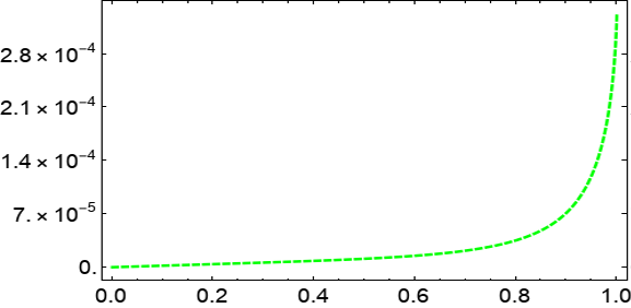
Figure 1: The radial function $R(\xi)$ with $\alpha_{+}=30$ and $\beta=30$ is shown to have an increasing profile towards LC with respect to the normalized radial distance $\xi$.

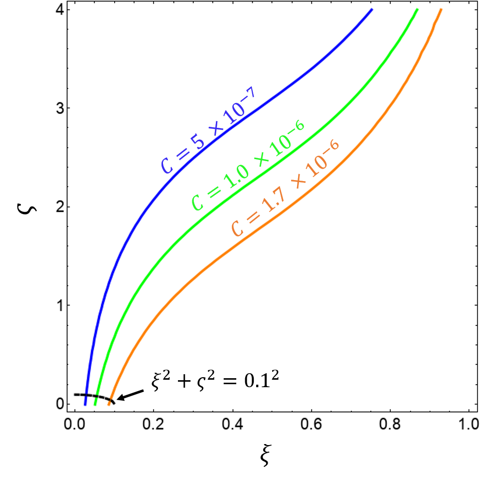
Figure 2: A set of poloidal field lines with $m=1$ originating from the neutron star with $\Psi(\xi,\varsigma)=C$ for an open magnetosphere is shown with $\xi_{ns}=0.1$.

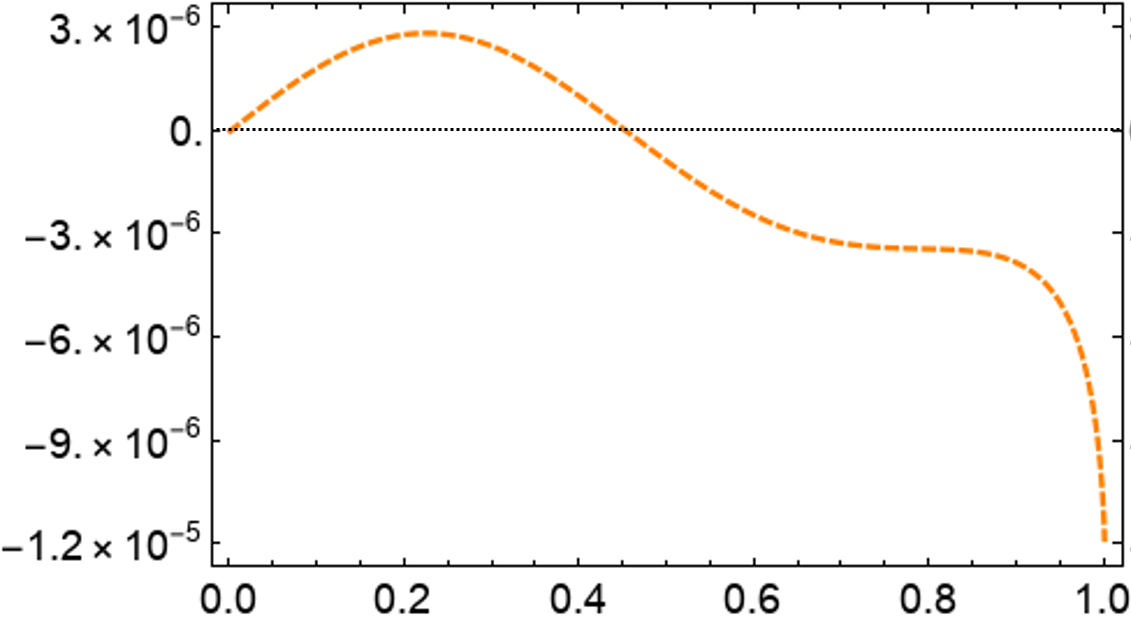
Figure 3: The radial function $R(\xi)$ with $\alpha_{+}=80$ and $\beta=30$ is shown to have an oscillatory profile before reaching LC with respect to the normalized radial distance $\xi$.

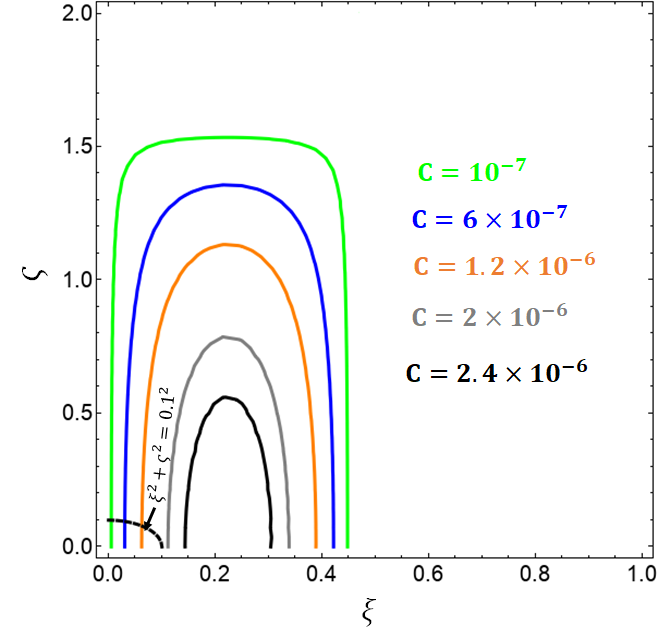
Figure 4: A set of poloidal field lines with $m=1$ originating from the neutron star with $\Psi(\xi,\varsigma)=C$ for a closed magnetosphere is shown with $\xi_{ns}=0.1$.

Now, let us consider the upper sign of Eq. 13 with $Z_{a}(\varsigma)$ of Eq. 18. With either $\partial Z_{a}(\varsigma)/\partial\varsigma=0$ at $\varsigma=0$ or the boundary condition $R(\xi)=\xi^{2}$ around $\xi=0$, we have $B_{r}=0$ at the center. We therefore have an axial magnetic field on the axis for unipolar induction. The corresponding upper sign of Eq. 17 for $R(\xi)$ with $\alpha_{-}=80$ and $\beta=30$ and $\alpha_{-}/\beta=8/3$ is plotted in Fig.3 showing the competition between the sinusoidal and the singular terms. This figure shows a local maximum $\xi^{*}_{0}$ bounded by a null point $\xi^{*}_{1}$, which is a separatrix for the closed configuration, before reaching LC asymptotically. A corresponding set of poloidal field lines

$$\Psi(\xi,\varsigma)\,=\,R(\xi)Z_{a}(\varsigma)\,=\,R(\xi)\cos m\varsigma\,=\,C\,\,\,,$$ (23)

is shown in Fig.4 with $m=1$ indicating a closed magnetosphere within the null point around $\xi=0.45$ where $R(\xi)=0$. To do this closed magnetosphere, we need only $\cos m\varsigma$ over $0<\varsigma<\pi/2$. Naturally, the highly exaggerated dimension with $\xi_{ns}=0.1$ of the open and closed magnetospheres is for illustration purposes. Increasing the contour value $C$, the closed poloidal field line would be detached from the pulsar surface. Further increasing $C$, more magnetic contours would be generated within earlier ones until reaching the magnetic axis around $\xi=0.23$ where $dR(\xi)/d\xi=0$. We remark that we have constructed the open and closed magnetospheres bounded by LC using an axial magnetic field on the $z$ axis as the boundary condition. Should we choose a dipole source with infinitely dense field lines at the stellar center, we would get the familiar closed configuration up to LC.

5 Revised Goldreich Julian Condition - Magnetosphere Dynamics

We have solved the pulsar equation, Eq. 8, for two equilibrium configurations. We remark that the pulsar equation is just the result of the equation of motion with the inertial term neglected for force-free field equilibrium coupled with the Maxwell equations. This equation by itself is model independent, and it depends on how the other physical variables are defined, such as the charge density, current density, and others. We note that the Ampere law provides the curvature of $\vec{B}$ in the presence of a current density $\vec{J}$. In a conductor, current density can be generated in the presence of an electromotive force, or by rotating it under an external magnetic field. In a magnetically confined MHD plasma, current can be generated by the guiding center drifts of the electron and ion species due to the magnetic curvature and gradient (Thompson, 1962; Schmidt, 1966; Jackson, 1975). We recall that in a uniform magnetic field, charge particles follow a circular gyro motion along the magnetic field lines according to the equation of motion. In the presence of a force transverse to the magnetic field, such as a centrifugal force due to curvature, and an inhomogeneous magnetic field, etc., the circular gyro motion will be transformed into a slowly displacing cycloid across the field lines, such that the gyro guiding center presents a transverse drift. These drifts are given by

$$\vec{v}_{Rc}\,=\,+{2\epsilon_{\parallel}\over q}{1\over B^{2}}({\vec{R}_{c}\over R_{c}^{2}}\times\vec{B})\,\,\,,$$ (24)

$$\vec{v}_{\nabla B}\,=\,-{\epsilon_{\perp}\over q}{1\over B^{2}}({\nabla B\over B}\times\vec{B})\,\,\,,$$ (25)

where $\epsilon_{\parallel}=mv_{\parallel}^{2}/2$ and $\epsilon_{\perp}=mv_{\perp}^{2}/2$ are the charge particle energies (temperature) parallel and perpendicular to the magnetic field. Therefore, these drifts are mass dependent as well as field dependent. The direction of these drifts depends on the sign of charge q, thus electrons and ions go in opposite direction generating a current,

$$\vec{J}\,=\,\rho_{q}^{*}\vec{v}_{current}\,=\,\rho_{q}^{*}(\vec{v}_{Rc}+\vec{v}_{\nabla B})\,=\,en(\vec{v}_{Rc}+\vec{v}_{\nabla B})\,\,\,,$$ (26)

where $\rho_{q}^{*}=en$ is the current generating charge density with all charged particles taking part. In the pulsar magnetosphere, the dominant part is the electron-positron plasma $n_{ep}$ plus the uploaded charges. Furthermore $\vec{v}_{current}$ is the current generating flow. As a result, the plasma drifts generate a current density $\vec{J}$ that feeds back to the magnetic field $\vec{B}$ through the Ampere law. We can now evaluate the Coulomb force space charge density

$$\rho_{q}\,=\,\epsilon_{0}\nabla\cdot\vec{E}\,=\,-\epsilon_{0}\nabla\cdot(\vec{v}_{E}\times\vec{B})\,=\,\epsilon_{0}(\vec{v}_{E}\cdot\mu_{0}\vec{J}-\vec{B}\cdot\nabla\times\vec{v}_{E})\,\,\,,$$

which can be written as

$$[\rho_{q}-\epsilon_{0}\mu_{0}\vec{v}_{E}\cdot\vec{J}]\,=\,-\epsilon_{0}\vec{B}\cdot\nabla\times\vec{v}_{E}\,\,\,.$$ (27)

By using Eq. 26, we then have

$$[\rho_{q}-\epsilon_{0}\mu_{0}\rho_{q}^{*}\vec{v}_{E}\cdot\vec{v}_{current}]\,=\,-\epsilon_{0}\vec{B}\cdot\nabla\times\vec{v}_{E}\,=\,-2\epsilon_{0}\vec{B}\cdot\vec{\Omega}_{0}\,=\,-2\epsilon_{0}B_{z}\Omega_{0}\,\,\,,$$ (28)

where the last equality is evaluated through $\vec{v}_{E}=r\Omega_{0}\hat{\phi}$.

Without considering the electron-positron plasma, Goldreich & Julian (1969) had derived a condition for the space charge density (their Eq.8) that read

$$\vec{J}\,=\,\rho_{q}^{*}\vec{v}_{current}\,=\,\rho_{q}^{*}\vec{v}\,=\,\pm en\vec{v}\,\,\,,$$ (29)

$$(1-\epsilon_{0}\mu_{0}v^{2})\rho_{q}^{*}\,=\,-2\epsilon_{0}\vec{B}\cdot\vec{\Omega}_{0}\,=\,-2\epsilon_{0}B_{z}\Omega_{0}\,\,\,.$$ (30)

They had denoted $\vec{v}$ as the plasma flow velocity, equivalent to $\vec{v}_{E}$, but this plasma flow velocity was also the current generating velocity, as in Eq. 29. Current flow was generated by plasma flow because the positive and negative plasmas were spatially separated in their model. The closed magnetosphere in the equatorial region was generated by the positive plasma with $\rho_{q}^{*}>0$. As for the open magnetosphere, it was generated by the open field lines of the negative plasma in the polar region plus part of the positive plasma in the intermediate region. The direction of the poloidal current flow along these open field lines was driven by the potential difference between the pulsar surface and the floating potential in the interstellar space, with a null line (null current flow) separating the inflow and outflow currents. In this charge separated model, all the charges took part in generating current through the plasma flow rendering $\vec{J}=\pm en\vec{v}=\rho_{q}^{*}\vec{v}$. As a result, the charge density of the Coulomb force $\rho_{q}\vec{E}=\pm en\vec{E}$ and the charge density of current generation $\vec{J}=\rho_{q}^{*}\vec{v}=\pm en\vec{v}$ were the same, $\rho_{q}=\rho_{q}^{*}=\pm en$, contrary to the $\rho_{q}$ of Eq. 1. Applying Eq. 30 to the closed equatorial magnetosphere with $\rho_{q}=\rho_{q}^{*}=+en>0$ and with the bracket multiplying $\rho_{q}^{*}$ on the left side always positive, this celebrated GJ condition indicated $B_{z}<0$ always. Thus the closed positively charged equatorial field lines remained closed and hence the term ¨dead zone¨, in contrast to the open field lines. For this reason, Eq. 30 described the stability of the positively charged closed pulsar magnetosphere.

Currently, although the magnetosphere plasma is regarded as a MHD plasma, the notion of a dead zone closed magnetosphere has persisted in MHD descriptions, and Eq. 28 appears to be compatible to Eq. 30 showing the dead zone. But it is not for two reasons. First, under the present description of a MHD plasma, with an electron-positron background plasma plus the uploaded unipolar pumped surface charges, the center of mass flow $\vec{v}_{E}$ of a MHD plasma does not generate current because the electrons and ions drift in the same direction, only the current generating flows of Eq. 24 and Eq. 25 are responsible for current. This is in contrast with the charge separated plasma model of Eq. 29 where plasma current is generated by charged plasma flow with $\rho_{q}=\pm en$. Second, the charge density of the Coulomb force in Eq. 1 is given by $\rho_{q}=\pm e\Delta n$. On the other hand, for the current density of Eq. 26 generated by drifts, all charged particles take part, but predominantly the electron-positron plasma $n_{ep}$, with $\rho_{q}^{*}=\pm en=\pm en_{ep}$. For these two reasons, in terms of $\rho_{q}$ of Eq. 1, the current density of Eq. 26 becomes

$$\vec{J}\,=\,\rho_{q}^{*}\vec{v}_{current}\,=\,\rho_{q}{n\over\Delta n}\vec{v}_{current}\,\,\,.$$ (31)

Consequently, Eq. 28 reads

$$[1-\epsilon_{0}\mu_{0}{n\over\Delta n}\vec{v}_{E}\cdot\vec{v}_{current}]\rho_{q}\,=\,-2\epsilon_{0}B_{z}\Omega_{0}\,\,\,.$$ (32)

Although the current generating drift velocity is quite slow, in the presence of the ${n/\Delta n}$ factor in Eq. 32, the closed magnetosphere within LC could open up, with $B_{z}>0$, to a LC guided jet as the electron-positron plasma density in the magnetosphere builds up. Thus the pulsar magnetic field re-establishes the axial field configuration, and the whole cycle starts anew.

6 Conclusions

Considering the neutron star as a superconductor rotating under a stationary axial magnetic field, instead of a dipole field, the unipolar induction continuously pumps charges to the pulsar surface according to their signs and sets up a potential distribution on the surface. These charges are uploaded to the magnetosphere along the magnetic field lines $\vec{B}$ to keep the surface charges in steady state and to generate a transverse electric field $\vec{E}$ across the field lines setting the plasma in motion with the $\vec{E}\times\vec{B}$ drift. Together with the electron-positron plasma in the magnetosphere, they generate a unique MHD plasma for the pulsar magnetosphere which is characterized by the Coulomb force charge density $\rho_{q}=\pm e\Delta n$ and the plasma current charge density $\rho_{q}^{*}=en$. Taking into consideration of the singularity, we have solved the pulsar equation for an open and a closed LC guided magnetosphere through a separation function with two parameters $(k^{2},\,m^{2})$. By choosing one set of parameters such that $R(\xi)$ is an increasing function asymptotically towards LC, we have constructed the polar jet configuration with $(\alpha_{+},\,\beta)$. The angular momentum of the toroidal $\vec{E}\times\vec{B}$ plasma drift collimates the jet making it stable over its lifetime. While with another set of parameters such that $R(\xi)$ goes through a maximum before approaching LC, we have also constructed the closed configuration with $(\alpha_{-},\,\beta)$. These two configurations reinforce the magnetosphere polar jet structure first pioneered by Sulkanen & Lovelace (1990). By distinguishing between the Coulomb force charge density $\rho_{q}$ and the plasma current charge density $\rho_{q}^{*}$, and between the center of mass flow $\vec{v}_{E}$ and the current generating flow $\vec{v}_{current}$, the celebrated GJ condition for the closed magnetosphere is revised, which shows that the closed magnetosphere could open as the electron-positron plasma density builds up. Consequently, the pulsar magnetosphere alternates between the closed and open configurations due to magnetosphere dynamics, releasing the stored magnetosphere energy along the pulsar axis periodically.

Funding

This research did not receive funding.

References

- Beskin & Malyshkin (1998) Beskin, V.S. & Malyshkin, L.M., 1998. On the self-consistent model of an axisymmetric radio pulsar magnetosphere, MNRAS, 298, 847-853.
- Beskin et al. (1993) Beskin, V.S., Gurevich, A.V., Istomin, Ya.N. 1993. Physics of the Pulsar Magnetosphere, Cambridge University Press, Cambridge.
- Contopoulos (2005) Contopoulos, I., 2005. The coughing pulsar magnetosphere, A&A, 442, 579-586.
- Contopoulos et al. (1999) Contopoulos, I., Kazanas, D., & Fendt, C., 1999. The axisymmetric pulsar magnetosphere, ApJ, 511, 351-358.
- Goldreich & Julian (1969) Goldreich, P. & Julian, W.H., 1969. Pulsar Electrodynamics, ApJ, 157, 869-880.
- Goodwin et al. (2004) Goodwin, S.P., Mestel, J., Mestel, L., & Wright, G.A.E., 2004. An idealized pulsar magnetosphere : the relativistic force-free approximation, MNRAS, 349, 213-224.
- Gruzinov (2005) Gruzinov, A., 2005. Power of an axisymmetric pulsar, Phys. Rev. Lett., 94, 021101.
- Jackson (1975) Jackson, J.D., 1975. Classical electrodynamics, Chapter 12, John Wiley & Sons, New York.
- Mestel & Wang (1979) Mestel, L. & Wang, Y.M., 1979. The axisymmetric pulsar magnetosphere - II, MNRAS, 188, 799-812.
- Mestel (1999) Mestel L. 1999. Stellar Magnetism, Clarendon Press, Oxford.
- Michel (1973) Michel, F.C., 1973. Rotating magnetosphere: A simple relativistic model, ApJ, 180, 207-225.
- Michel (1990) Michel, F.C., 1990. Theory of Neutron Star Magnetospheres, The University of Chicago Press, Chicago.
- Morse & Feshbach (1953) Morse, P.M., Feshbach, H., 1953. Methods of Theoretical Physics, Chapter 5, p.516, Part I, McGraw-Hill, New York.
- Ogura & Kojima (2003) Ogura, J. & Kojima, Y., 2003. Some properties of an axisymmetric pulsar magnetosphere constructed by numerical claculations, Prog. Theo. Phys., 109, 619-630.
- Okamoto (1974) Okamoto, I., 1974. Force-free pulsar magnetosphere - I. The steady axisymmetric theory for the charge-separated plasma, MNRAS, 167, 457-474.
- Petrova (2013) Petrova, S.A., 2013. On the global structure of pulsar force-free magnetosphere, ApJ, 764, 129(5pp).
- Scharlemann & Wagoner (1973) Scharlemann, E.T. & Wagoner, R.V., 1973. Aligned rotating magnetospheres. I. General analysis, ApJ, 182, 951-960.
- Schmidt (1966) Schmidt, G., 1966. Physics of high temperature plasmas, Chapter II, Academic Press, New York.
- Sturrock (1971) Sturrock, P.A., 1971. A model of pulsars, ApJ, 164, 529-556.
- Sulkanen & Lovelace (1990) Sulkanen, M.E. & Lovelace, R.V.E., 1990. Pulsar magnetospheres with jets, ApJ, 350, 732-744.
- Thompson (1962) Thompson, W.B., 1962. An introduction to plasma physics, Chapter 7, Addison-Wesley, London.
- Timokhin (2006) Timokhin, A.N., 2006. On the force-free magnetosphere of an aligned rotator, MNRAS, 368, 1055-1072.