Two-view Graph Neural Networks
for Knowledge Graph Completion

Abstract

We present an effective graph neural network (GNN)-based knowledge graph embedding model, which we name WGE, to capture entity- and relation-focused graph structures. Given a knowledge graph, WGE builds a single undirected entity-focused graph that views entities as nodes. WGE also constructs another single undirected graph from relation-focused constraints, which views entities and relations as nodes. WGE then proposes a GNN-based architecture to better learn vector representations of entities and relations from these two single entity- and relation-focused graphs. WGE feeds the learned entity and relation representations into a weighted score function to return the triple scores for knowledge graph completion. Experimental results show that WGE outperforms strong baselines on seven benchmark datasets for knowledge graph completion.

1 Introduction

A knowledge graph (KG) is a network of entity nodes and relationship edges, which can be represented as a collection of triples in the form of (h, r, t), wherein each triple (h, r, t) represents a relation $r$ between a head entity $h$ and a tail entity $t$. Here, entities are real-world things or objects such as music tracks, movies persons, organizations, places and the like, while each relation type determines a certain relationship between entities. KGs are used in many commercial applications, e.g. in such search engines as Google, Microsoft’s Bing and Facebook’s Graph search. They also are useful resources for many natural language processing tasks such as co-reference resolution [27, 8], semantic parsing [18, 2] and question answering [10, 9]. However, an issue is that KGs are often incomplete, i.e., missing a lot of valid triples [4, 23]. For an example of a specific application, question answering systems based on incomplete KGs would not provide correct answers given correctly interpreted input queries. Thus, much work has been devoted towards KG completion to perform link prediction in KGs. In particular, many KG embedding models have been proposed to predict whether a triple not in KGs is likely to be valid or not, e.g., TransE [3], DistMult [37], ComplEx [33] and QuatE [39]. These KG embedding models aim to learn vector representations for entities and relations and define a score function such that valid triples have higher scores than invalid ones [23, 40], e.g., the score of the valid triple (Sydney, city_in, Australia) is higher than the score of the invalid one (Sydney, city_in, Vietnam).

Recently, several KG completion works have adapted graph neural networks (GNNs) using an encoder-decoder architecture, e.g., R-GCN [30] and CompGCN [34]. In general, the encoder module customizes GNNs to update vector representations of entities and relations. Then, the decoder module employs an existing score function to return the triple score [3, 37, 33, 7, 20, 6, 5]. For example, R-GCN adapts Graph Convolutional Networks (GCNs) [17] to construct a specific encoder to update only entity embeddings. CompGCN modifies GCNs to use composition operations between entities and relations in the encoder module. Note that these existing GNN-based KG embedding models mainly consider capturing the graph structure surrounding entities as relation representations are used to update the entity embeddings only (as shown in Equations 3, 5 and 6; and see the last paragraph of Section 2 for a detailed discussion). Therefore, they might miss covering potentially useful information on relation structure.

To this end, we propose a new KG embedding model—named WGE that is equivalent to VVGE to abbreviate Two-View Graph Embedding—to leverage GNNs to capture both entity-focused graph structure and relation-focused graph structure for KG completion. In particular, WGE transforms a given KG into two views. The first view—a single undirected entity-focused graph—only includes entities as nodes to provide the entity neighborhood information. The second view—a single undirected relation-focused graph—considers both entities and relations as nodes, constructed from constraints (subjective relation, predicate entity, objective relation) e.g. (born_in, Sydney, city_in), to attain the potential dependence between two neighborhood relations. For instance, the knowledge about a potential dependence between “born_in” and “city_in” could be relevant for predicting some other relationship, e.g. “nationality” or “country of citizenship”. Then WGE introduces a new GNN-based encoder module that directly takes these two graph views as input to better update entity and relation embeddings. WGE feeds the entity and relation embeddings into its decoder module that uses a weighted score function to return the triple scores for KG completion. In summary, our contributions are as follows:

• We present WGE for KG completion, that first proposes to transform a given KG into entity- and relation-focused graph structures and then introduces a new encoder architecture to learn entity and relation embeddings from these two graph structures.

• To verify model effectiveness, we conduct extensive experiments to compare our WGE with other strong GNN-based baselines on seven benchmark datasets, including FB15K-237 [32] and six new and difficult datasets of CoDEx-S, CoDEx-M, CoDEx-L, LitWD1K, LitWD19K and LitWD48K [28, 11]. The experiments show that WGE outperforms the GNN-based baselines and other competitive KG embedding models on these seven datasets.

2 Related work

Recently, GNNs become a central strand to learn low-dimensional continuous embeddings for nodes and graphs [29, 14]. GNNs provide faster and more practical training and state-of-the-art results on benchmark datasets for downstream tasks [36, 38]. In general, GNNs update the vector representation of each node by transforming and aggregating the vector representations of its neighbors [17, 13, 35, 21, 22].

We represent each graph $\mathcal{G}=\left(\mathcal{V},\mathcal{E}\right)$, where $\mathcal{V}$ is a set of nodes; and $\mathcal{E}$ is a set of edges. Given a graph $\mathcal{G}$, we formulate GNNs as follows:

$$\boldsymbol{\mathsf{h}}_{\mathsf{v}}^{(k+1)}=\textsc{Aggregation}\left(\left\{\boldsymbol{\mathsf{h}}^{(k)}_{\mathsf{u}}\right\}_{\mathsf{u}\in\mathcal{N}_{\mathsf{v}}\cup\left\{\mathsf{v}\right\}}\right)$$ (1)

where $\boldsymbol{\mathsf{h}}_{\mathsf{v}}^{(k)}$ is the vector representation of node $\mathsf{v}$ at the $k$-th layer; and $\mathcal{N}_{\mathsf{v}}$ is the set of neighbours of node $\mathsf{v}$.

There have been many designs for the Aggregation functions. The widely-used one is introduced in Graph Convolutional Networks (GCNs) [17] as:

$$\boldsymbol{\mathsf{h}}_{\mathsf{v}}^{(k+1)}=\mathsf{g}\left(\sum_{\mathsf{u}\in\mathcal{N}_{\mathsf{v}}\cup\left\{\mathsf{v}\right\}}a_{\mathsf{v},\mathsf{u}}\boldsymbol{W}^{(k)}\boldsymbol{\mathsf{h}}_{\mathsf{u}}^{(k)}\right),\forall\mathsf{v}\in\mathcal{V}$$ (2)

where $\mathsf{g}$ is a nonlinear activation function such as $\mathsf{ReLU}$; $\boldsymbol{W}^{(k)}$ is a weight matrix at the $k$-th layer; and $a_{\mathsf{v},\mathsf{u}}$ is an edge constant between nodes $\mathsf{v}$ and $\mathsf{u}$ in the re-normalized adjacency matrix $\tilde{\textbf{D}}^{-\frac{1}{2}}\tilde{\textbf{A}}\tilde{\textbf{D}}^{-\frac{1}{2}}$, wherein $\tilde{\textbf{A}}=\textbf{A}+\textbf{I}$ where A is the adjacency matrix, I is the identity matrix, and $\tilde{\textbf{D}}$ is the diagonal node degree matrix of $\tilde{\textbf{A}}$.

It is worth mentioning that several KG embedding approaches have been proposed to adapt GNNs for knowledge graph link prediction [30, 31, 34]. For example, R-GCN [30] modifies the basic form of GCNs to introduce a specific encoder to update entity embeddings:

$$\boldsymbol{\mathsf{h}}_{\mathsf{e}}^{(k+1)}=\mathsf{g}\left(\sum_{r\in\mathcal{R}}\sum_{\mathsf{e^{\prime}}\in\mathcal{N}_{\mathsf{e}}^{r}}\frac{1}{|\mathcal{N}_{\mathsf{e}}^{r}|}\boldsymbol{W}_{r}^{(k)}\boldsymbol{\mathsf{h}}_{\mathsf{e^{\prime}}}^{(k)}+\boldsymbol{W}^{(k)}\boldsymbol{\mathsf{h}}_{\mathsf{e}}^{(k)}\right)$$ (3)

where $\mathcal{R}$ is a set of relations in the KG; $\mathcal{N}_{\mathsf{e}}^{r}=\left\{e^{\prime}|(e,r,e^{\prime})\in\mathcal{T}\cup(e^{\prime},r,e)\in\mathcal{T}\right\}$ denotes the set of entity neighbors of entity $\mathsf{e}$ via relation edge $r$, wherein $\mathcal{T}$ denotes the set of knowledge graph triples; and $\boldsymbol{W}_{r}^{(k)}$ is a weight transformation matrix associated with $r$ at the $k$-th layer. Then R-GCN uses DistMult [37] as its decoder module to compute the score of (h, r, t) as:

$$f\left(h,r,t\right)=\left<\boldsymbol{\mathsf{h}}_{h}^{(K)},\boldsymbol{v}_{r},\boldsymbol{\mathsf{h}}_{t}^{(K)}\right>$$ (4)

where $\boldsymbol{\mathsf{h}}_{h}^{(K)}$ and $\boldsymbol{\mathsf{h}}_{t}^{(K)}$ are output vectors taken from the last layer of the encoder module; $\boldsymbol{v}_{r}$ denotes the embedding of relation $r$; and $\left<\right>$ denotes a multiple-linear dot product $\left<\boldsymbol{\mathsf{a}},\boldsymbol{\mathsf{b}},\boldsymbol{\mathsf{c}}\right>=\sum_{i}^{n}\boldsymbol{\mathsf{a}}_{i}\times\boldsymbol{\mathsf{b}}_{i}\times\boldsymbol{\mathsf{c}}_{i}$.

CompGCN [34] also customizes GCNs to consider composition operations between entities and relations in the encoder module as follows:

$$\boldsymbol{\mathsf{h}}_{\mathsf{e}}^{(k+1)} =\mathsf{g}\left(\sum_{(\mathsf{e^{\prime}},r)\in\mathcal{N}_{\mathsf{e}}}\boldsymbol{W}_{\mathsf{type}(r)}^{(k)}\phi\left(\boldsymbol{\mathsf{h}}_{\mathsf{e^{\prime}}}^{(k)},\boldsymbol{\mathsf{h}}_{r}^{(k)}\right)\right)$$ (5)

$$\boldsymbol{\mathsf{h}}_{r}^{(k+1)} =\boldsymbol{W}^{(k)}\boldsymbol{\mathsf{h}}_{r}^{(k)}$$ (6)

where $\mathcal{N}_{\mathsf{e}}=\left\{(e^{\prime},r)|(e,r,e^{\prime})\in\mathcal{T}\cup(e^{\prime},r,e)\in\mathcal{T}\right\}$ is the neighboring entity-relation pair set of entity $e$; and $\boldsymbol{W}_{\mathsf{type}(r)}^{(k)}$ denotes relation-type specific weight matrix. CompGCN explores the composition functions ($\phi$) inspired from TransE [3], DistMult, and HolE [24]. Then CompGCN uses ConvE [7] as the decoder module.

The existing GNN-based KG embedding models, e.g. R-GCN and CompGCN, mainly capture the graph structure surrounding entities. That is, as shown in Equations 3, 5 and 6, a relation’s representation is not directly used to update another relation’s representation and is only used to update entity embeddings, while entity embeddings are not used to update relation representations. Thus, these models might miss covering potentially useful relation structure information that is illustrated by the example (born_in, Sydney, city_in) in Section 1.

3 Our model WGE

A knowledge graph $G=\left\{\mathcal{V},\mathcal{R},\mathcal{T}\right\}$ can be represented as a collection of factual valid triples (head entity, relation, tail entity) denoted as $(h,r,t)\in\mathcal{T}$ with $h,t\in{\mathcal{V}}$ and $r\in\mathcal{R}$, wherein $\mathcal{V}$, $\mathcal{R}$ and $\mathcal{T}$ denote the sets of entities, relations and triples, respectively.

To better capture the graph structure, as illustrated in Figure 1, we introduce WGE as follows: (i) WGE transforms a given KG into two views: a single undirected entity-focused graph and a single undirected relation-focused graph. (ii) WGE introduces a new encoder architecture to update vector representations of entities and relations based on these two single graphs. (iii) WGE utilizes a weighted score function as the decoder module to compute the triple scores.

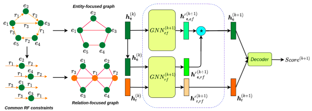
Figure 1: An illustration of our proposed WGE. Here, $\boldsymbol{h}^{(k)}_{\mathsf{e}}$ and $\boldsymbol{h}^{(k)}_{r}$ the vector representations of the entity $\mathsf{e}$ and the relation $r$ at $k$-th layer of the encoder module, are computed following Equation 13.

3.1 Two-view construction

3.1.1 Entity-focused view 

WGE aims to obtain the entity neighborhood information. Thus, given a KG $G$, WGE constructs a single undirected graph $\mathcal{G}_{ef}$ viewing entities as individual nodes. Here, $\mathcal{G}_{ef}=\left\{\mathcal{V}_{ef},\mathcal{E}_{ef}\right\}$, wherein $\mathcal{V}_{ef}$ is the set of nodes and $\mathcal{E}_{ef}$ is the set of edges. The number of nodes in $\mathcal{G}_{ef}$ is equal to the number of entities in $G$, i.e., $|\mathcal{V}_{ef}|=|\mathcal{V}|$. In particular, for each triple $(h,r,t)$ in $G$, entities $h$ and $t$ become individual nodes in $\mathcal{G}_{ef}$ with an edge between them, as illustrated in Figure 1. Here, $\mathcal{G}_{ef}$ is associated with an adjacency matrix $\boldsymbol{A}_{ef}$:

$$\boldsymbol{A}_{ef}(\mathsf{v},\mathsf{u})=\left\{\begin{array}[]{l}1\ \ \ \text{if there is an edge between entity nodes $\mathsf{v}$ and $\mathsf{u}$}\\ 0\ \ \ \text{otherwise }\end{array}\right.$$ (7)

3.1.2 Relation-focused view 

WGE also aims to attain the potential dependence between two neighborhood relations (e.g. “child_of” and “spouse”) to enhance learning representations. To do that, from $G$, our WGE extracts relation-focused (RF) constraints in the form of (subjective relation, predicate entity, objective relation), denoted as $(r_{s},e_{p},r_{o})$, wherein $e_{p}$ is the tail entity for the relation $r_{s}$ and also the head entity for the relation $r_{o}$, e.g. (born_in, Sydney, city_in). Here, WGE keeps a certain fraction $\beta$ of common RF constraints based on ranking how often two relations $r_{s}$ and $r_{o}$ co-appear in all extracted RF ones. Then, WGE transforms those common obtained RF constraints into a single undirected relation-focused graph $\mathcal{G}_{rf}=\left\{\mathcal{V}_{rf},\mathcal{E}_{rf}\right\}$ that views both entities and relations as individual nodes, wherein $\mathcal{V}_{rf}$ is the set of entity and relation nodes, $\mathcal{E}_{rf}$ is the set of edges. For example, as shown in Figure 1, given an RF constraint $(r_{1},e_{2},r_{2})$, WGE considers $r_{1}$, $e_{2}$, and $r_{2}$ as individual nodes in $\mathcal{G}_{rf}$ with edges among them. $\mathcal{G}_{rf}$ is associated with an adjacency matrix $\boldsymbol{A}_{rf}$:

$$\boldsymbol{A}_{rf}(\mathsf{v},\mathsf{u})=\left\{\begin{array}[]{l}1\ \ \ \text{if there is an edge between nodes $\mathsf{v}$ and $\mathsf{u}$}\\ 0\ \ \ \text{otherwise }\end{array}\right.$$ (8)

3.2 Encoder module

Given a single graph $\mathcal{G}=\left(\mathcal{V},\mathcal{E}\right)$, we might adopt vanilla GNNs or GCNs directly on $\mathcal{G}$ and its adjacency matrix $\boldsymbol{A}$ to learn node embeddings. Recently, QGNN—Quaternion Graph Neural Network [21]—has been proposed to learn node embeddings in the quaternion space as follows:

$$\boldsymbol{h}_{\mathsf{v}}^{(k+1),Q}=\mathsf{g}\left(\sum_{\mathsf{u}\in\mathcal{N}_{\mathsf{v}}\cup\left\{\mathsf{v}\right\}}\mathsf{a}_{\mathsf{v},\mathsf{u}}\boldsymbol{W}^{(k),Q}\otimes\boldsymbol{h}_{\mathsf{u}}^{(k),Q}\right)$$ (9)

where the superscript ^Q denotes the quaternion space; $k$ is the layer index; $\mathcal{N}_{\mathsf{v}}$ is the set of neighbors of node $\mathsf{v}$; $\boldsymbol{W}^{(k),Q}$ is a quaternion weight matrix; $\otimes$ denotes the Hamilton product; and $\mathsf{g}$ is a nonlinear activation function such as $\mathsf{tanh}$; $\boldsymbol{h}_{\mathsf{u}}^{(0),Q}\in\mathbb{H}^{n}$ is an input embedding vector for node $\mathsf{u}$, which is randomly initialized and updated during training; and $\mathsf{a}_{\mathsf{v},\mathsf{u}}$ is an edge constant between nodes $\mathsf{v}$ and $\mathsf{u}$ in the Laplacian re-normalized adjacency matrix $\tilde{\textbf{D}}^{-\frac{1}{2}}\tilde{\textbf{A}}\tilde{\textbf{D}}^{-\frac{1}{2}}$ with $\tilde{\textbf{A}}=\boldsymbol{A}+\textbf{I}$, where $\boldsymbol{A}$ is the adjacency matrix, I is the identity matrix, and $\tilde{\textbf{D}}$ is the diagonal node degree matrix of $\tilde{\textbf{A}}$. See quaternion algebra background in the Appendix. QGNN has demonstrated its superior performances for downstream tasks such as graph classification and node classification.

Our WGE thus proposes a new encoder architecture to learn entity and relation vector representations based on two different QGNNs, as illustrated in Figure 1. This new encoder aims to capture both entity- and relation-focused graph structures to better update vector representations for entities and relations as follows:

$$\boldsymbol{h^{\prime}}_{\mathsf{v},ef}^{(k+1),Q}=\mathsf{g}\left(\sum_{\mathsf{u}\in\mathcal{N}_{\mathsf{v}}\cup\left\{\mathsf{v}\right\}}\mathsf{a}_{\mathsf{v},\mathsf{u},ef}\boldsymbol{W}_{ef}^{(k),Q}\otimes\boldsymbol{h}_{\mathsf{u},ef}^{(k),Q}\right)$$ (10)

where the subscript _ef denotes for QGNN on the entity-focused graph $\mathcal{G}_{ef}$, and we define $\boldsymbol{h}_{\mathsf{u},ef}^{(k),Q}$ as:

$$\boldsymbol{h}_{\mathsf{u},ef}^{(k),Q}=\boldsymbol{h^{\prime}}_{\mathsf{u},ef}^{(k),Q}*\boldsymbol{h^{\prime}}_{\mathsf{u},rf}^{(k),Q}$$ (11)

where $*$ denotes a quaternion element-wise product, and $\boldsymbol{h^{\prime}}_{\mathsf{u},rf}^{(k),Q}$ is computed following the Equation 12:

$$\boldsymbol{h^{\prime}}_{\mathsf{v},rf}^{(k+1),Q}=\mathsf{g}\left(\sum_{\mathsf{u}\in\mathcal{N}_{\mathsf{v}}\cup\left\{\mathsf{v}\right\}}\mathsf{a}_{\mathsf{v},\mathsf{u},rf}\boldsymbol{W}_{rf}^{(k),Q}\otimes\boldsymbol{h}_{\mathsf{u}}^{(k),Q}\right)$$ (12)

where the subscript _rf denotes for QGNN on the relation-focused graph $\mathcal{G}_{rf}$. We define $\boldsymbol{h}_{\mathsf{u}}^{(k),Q}$ as:

$$\boldsymbol{h}_{\mathsf{u}}^{(k),Q}=\left\{\begin{array}[]{l}\boldsymbol{h}_{\mathsf{u},ef}^{(k),Q}\ \ \ \text{if $\mathsf{u}$ is an entity node, as in Equation \ref{equa:equahuef} }\\ \\ \boldsymbol{h^{\prime}}_{\mathsf{u},rf}^{(k),Q}\ \ \ \text{if $\mathsf{u}$ is a relation node, following Equation \ref{equa:QGNNrf} }\end{array}\right.$$ (13)

WGE uses $\boldsymbol{h}_{\mathsf{e}}^{(k),Q}$ and $\boldsymbol{h}_{\mathsf{r}}^{(k),Q}$ as computed following Equation 13 as the vector representations for entity $\mathsf{e}$ and relation $\mathsf{r}$ at the $k$-th layer of our encoder module, respectively. These vectors will be used as input for the decoder module.

Note that our encoder module is not merely using such a GNN but proposes a new manner where the two GNNs interact with each other to jointly learn entity and relation representations from two graphs. This interaction is crucial and novel and is directly responsible for the good performance of our model, showing that two-view modeling helps produce better scores than single-view modeling (See our ablation study in Section 4.3).

3.3 Decoder module

As the encoder module learns quaternion entity and relation embeddings, WGE employs the quaternion KG embedding model QuatE [39] across all hidden layers of the encoder module to return a final score $f(h,r,t)$ for each triple $(h,r,t)$ as:

$$f_{k}(h,r,t) =\left(\boldsymbol{h}_{h}^{(k),Q}\otimes\boldsymbol{h}_{r}^{\triangleleft,(k),Q}\right)\bullet\boldsymbol{h}_{t}^{(k),Q}$$ (14)

$$f(h,r,t) =\sum_{k}\alpha_{k}f_{k}(h,r,t)$$ (15)

where $\alpha_{k}\in[0,1]$ is a fixed important weight of the $k$-th layer with $\sum_{k}\alpha_{k}=1$; $\boldsymbol{h}_{h}^{(k),Q}$, $\boldsymbol{h}_{r}^{(k),Q}$, and $\boldsymbol{h}_{t}^{(k),Q}$ are quaternion vectors taken from the $k$-th layer of the encoder; $\otimes$, ^◁ and $\bullet$ denote the Hamilton product, the normalized quaternion and the quaternion-inner product, respectively.

3.4 Objective function

We train WGE by using Adam [16] to optimize a weighted loss function as:

$$\mathcal{L}=-\sum_{\begin{subarray}{c}(h,r,t)\in\{\mathcal{T}\cup\mathcal{T}^{\prime}\}\end{subarray}}\sum_{k}\alpha_{k}\Big{(}l_{(h,r,t)}\log\big{(}p_{k}(h,r,t)\big{)}$$

$$\ \ \ \ \ \ \ \ \ \ \ \ \ \ \ \ \ \ \ \ +\big{(}1-l_{(h,r,t)}\big{)}\log\big{(}1-p_{k}(h,r,t)\big{)}\Big{)}$$ (16)

$$\text{in which, }l_{(h,r,t)}=\left\{\begin{array}[]{l}1\ \ \ \text{for }(h,r,t)\in\mathcal{T}\\ 0\ \ \ \text{for }(h,r,t)\in\mathcal{T}^{\prime}\end{array}\right.$$ (19)

$$\text{and }p_{k}(h,r,t)=\mathsf{sigmoid}\big{(}f_{k}(h,r,t)\big{)}$$

here, $\mathcal{T}$ and $\mathcal{T}^{\prime}$ are collections of valid and invalid triples, respectively. $\mathcal{T}^{\prime}$ is collected by corrupting valid triples in $\mathcal{T}$.

4 Experiments

We evaluate our proposed WGE for the KG completion task, i.e., link prediction [3], which aims to predict a missing entity given a relation with another entity, e.g., predicting a head entity $h$ given $(?,r,t)$ or predicting a tail entity $t$ given $(h,r,?)$. The results are calculated by ranking the scores produced by the score function $f$ on triples in the test set.

4.1 Setup

4.1.1 Datasets 

Recent works [28, 11] show that there are some quality issues with previous existing KG completion datasets. For example, a large percentage of relations in FB15K-237 [32] could be covered by a trivial frequency rule [28]. Hence, they introduce six new KG completion benchmarks, consisting of CoDEx-S, CoDEx-M, CoDEx-L, LitWD1K, LitWD19K and LitWD48K. These datasets are more difficult and cover more diverse and interpretable content than the previous ones. We use the six new challenging datasets as well as the FB15K-237 dataset to compare different models. The statistics of these datasets are presented in Table 1.

Table 1: Statistics of the experimental datasets.

Dataset	$|\mathcal{E}|$	$|\mathcal{R}|$	$\#$Triples
			Train	Valid	Test
CoDEx-S	2,034	42	32,888	1827	1828
CoDEx-M	17,050	51	185,584	10,310	10,311
CoDEx-L	77,951	69	551,193	30,622	30,622
LitWD1K	1,533	47	26,115	1,451	1,451
LitWD19K	18,986	182	260,039	14,447	14,447
LitWD48K	47,998	257	303,117	16,838	16,838
FB15K-237	14,541	237	272,115	17,535	20,466

4.1.2 Evaluation protocol 

Following the standard protocol [3], to generate corrupted triples for each test triple $(h,r,t)$, we replace either $h$ or $t$ by each of all other entities in turn. We also apply the “Filtered” setting protocol [3] to filter out before ranking any corrupted triples that appear in the KG. We then rank the valid test triple as well as the corrupted triples in descending order of their triple scores. We report standard evaluation metrics: mean reciprocal rank (MRR) and Hits@10 (i.e. the proportion of test triples for which the target entity is ranked in the top 10 predictions). Here, a higher MRR/Hits@10 score reflects a better prediction result.

4.1.3 Our model’s training protocol 

We implement our model using Pytorch [26]. We apply the standard Glorot initialization [12] for parameter initialization. We employ $\mathsf{tanh}$ for the nonlinear activation function $\mathsf{g}$. We use the Adam optimizer [16] to train our WGE model up to 3000 epochs on all datasets. We use a grid search to choose the number $K$ of hidden layers $\in\{1,2,3\}$, the Adam initial learning rate $\in\left\{1e^{-4},5e^{-4},1e^{-3},5e^{-3}\right\}$, the batch size $\in\left\{1024,2048,4096\right\}$, and the input dimension and hidden sizes of the QGNN hidden layers $\in\left\{32,64,128,256,512,1024\right\}$. For the decoder module, we perform a grid search to select its mixture weight value $\alpha_{0}\in\{0.3,0.6,0.9\}$, and fix the mixture weight values for the $K$ layers at $\alpha_{k}=\dfrac{1-\alpha_{0}}{K}$. For the percentage $\beta$ of kept RF constraints, we grid-search $\beta\in\{0.1,0.2,...,0.9\}$ for the CoDEx-S dataset, and the best value is $0.2$; then we use $\beta=0.2$ for all remaining datasets. We evaluate the MRR after every 10 training epochs on the validation set to select the best model checkpoint, and then apply the selected one to the test set.

4.1.4 Baselines’ training protocol 

For strong baseline models, we apply the same evaluation protocol. The training protocol is the same w.r.t. parameter initialization, the optimizer, the hidden layers, the initial learning rate values, the batch sizes and the number of training epochs as well as the best model checkpoint selection. We also use a model-specific configuration for each baseline. In particular, for TransE [3], ConvE [7], TuckER [1] and QuatE, we use grid search to choose the embedding dimension in {64, 128, 256, 512}. For the QGNN-based KG embedding model SimQGNN [21] that obtains state-of-the-art results on the CoDEx datasets, we successfully reproduce this model’s reported results using its optimal hyper-parameters. For R-GCN and CompGCN, we use 2 GCN layers and vary the embedding size of the GCN layer from {64, 128, 256, 512}. For WGE variants in the Ablation study, we also set the same dimension value for both the embedding size and the hidden size, wherein we vary the dimension value in {64, 128, 256, 512}.

Table 2: Experimental results on seven test sets. Hits@10 (H@10) is reported in %. The best scores are in bold, while the second best scores are in underline. The results of TransE [3], ComplEx [33], ConvE [7] and TuckER [1] on three CoDEx test sets are taken from [28]. The results of R-GCN [30] and CompGCN [34] and SimQGNN [21] on three CoDEx test sets are taken from [21]. The ComplEx results on three LitWD test sets are taken from [11]. The results of TransE, ComplEx, ConvE, R-GCN and CompGCN on the FB15K-237 test set are taken from [34]. The results of TuckER on FB15K-237 are taken from [1]. All results are reported using the same setup.

Method	CoDEx-S		CoDEx-M		CoDEx-L		LitWD1K		LitWD19K		LitWD48K		FB15K-237
	MRR	H@10	MRR	H@10	MRR	H@10	MRR	H@10	MRR	H@10	MRR	H@10	MRR	H@10
TransE	0.354	63.4	0.303	45.4	0.187	31.7	0.313	51.3	0.172	26.4	0.269	41.3	0.294	46.5
ComplEx	0.465	64.6	0.337	47.6	0.294	40.0	0.413	67.3	0.181	29.6	0.277	42.8	0.247	33.9
ConvE	0.444	63.5	0.318	46.4	0.303	42.0	0.477	71.4	0.310	45.1	0.372	54.0	0.325	50.1
TuckER	0.444	63.8	0.328	45.8	0.309	43.0	0.498	74.4	0.311	46.3	0.391	58.7	0.358	54.4
R-GCN	0.275	53.3	0.124	24.1	0.073	14.2	0.244	46.2	0.211	34.1	0.238	44.2	0.248	41.7
CompGCN	0.395	62.1	0.312	45.7	0.304	42.8	0.323	52.8	0.319	47.4	0.379	58.4	0.355	53.5
SimQGNN	0.435	65.2	0.323	47.7	0.310	43.7	0.518	75.1	0.308	46.9	0.350	57.6	0.339	51.8
QuatE	0.449	64.4	0.323	48.0	0.312	44.3	0.514	73.1	0.341	49.3	0.392	58.6	0.342	52.9
WGE	0.452	66.4	0.338	48.5	0.320	44.5	0.527	76.2	0.345	49.9	0.401	59.5	0.348	53.6

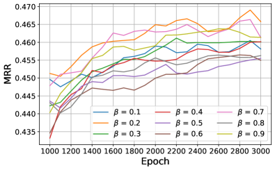
(a) Effects of the percentage $\beta$.

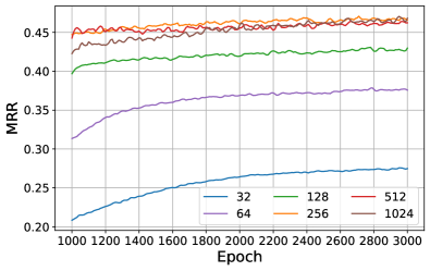
(b) Effects of the embedding sizes.

Figure 2: Effects of hyper-parameters on the CoDEx-S validation set.

4.2 Main results

Table 2 shows our results obtained for WGE and other strong baselines on seven experimental datasets. In general, our WGE obtains the highest MRR and Hits@10 scores on all three CoDEx and three LitDW challenge datasets (except the second highest MRR on CoDEx-S); and on FB15K-237, WGE obtains the third highest MRR and the second highest Hits@10. In particular, WGE gains substantial improvements compared to both R-GCN and CompGCN on all three CoDEx and three LitDW challenge datasets. Compared to the QGNN-based model SimQGNN, our WGE obtains 1.5% and 0.02 absolute higher Hits@10 and MRR scores averaged over all seven datasets than SimQGNN, respectively. We also find that QuatE obtains competitive performance scores when carefully tuning its hyper-parameters (e.g. generally outperforming SimQGNN), however, it is still surpassed by WGE by about 1.1+% and 0.01 on averaged Hits@10 and MRR, respectively.

4.2.1 Hyper-parameter sensitivity 

We present in Figures 2(a) and 2(b) the effects of essential hyper-parameters including the percentage $\beta$ of kept RF constraints and the embedding sizes on the CoDEx-S validation set.

• Percentage $\beta$ of kept RF constraints: As defined in Section 3.1, the hyper-parameter $\beta$ aims to determine the number of common RF constraints to be kept in the relation-focused graph. We visualize the MRR scores according to the value of $\beta$ in $\{0.1,0.2,...,0.9\}$ in Figure 2(a). We find that WGE performs best with $\beta=0.2$. Recall that the hyper-parameter $\beta=0.2$ is tuned on the CoDEx-S validation set only, and then used for all remaining datasets. Here, the hyper-parameter $\beta=0.2$ already helps our WGE to outperform strong baselines, as shown in Table 2. Our scores obtained on the remaining datasets are likely better if $\beta$ is also tuned on those datasets. A limitation of our approach is that the mechanism of selecting kept RF constraints in the Relation-focused view is based on the observed co-occurrence frequency between entities and relations. This might not be optimal as some entity-relation pairs can have important interactions regardless of their small number of co-occurrences as the observed KG is incomplete (the actual number of co-occurrences could be larger). In future work, we would design a soft scoring mechanism that gives a score for each entity-relation pair and be able to adaptively prune the graph during training.

• Embedding sizes: Figure 2(b) illustrates the performance differences of WGE when varying the embedding size in $\{32,64,128,256,512,1024\}$. Our WGE achieves the highest MRR when the embedding size is 256. We find that there are no substantial MRR gains when the size is larger than 256. We also observe similar findings for the remaining datasets.

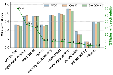
(a) Tail prediction on CoDEx-S.

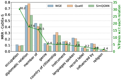
(b) Head prediction on CoDEx-S.

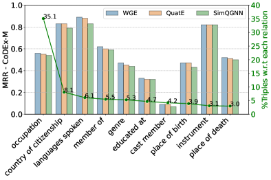
(c) Tail prediction on CoDEx-M.

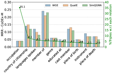
(d) Head prediction on CoDEx-M.

Figure 3: MRR on the CoDEx-S and CoDEx-M validation sets w.r.t each relation. The right y-axis is the percentage of triples corresponding to each relation.

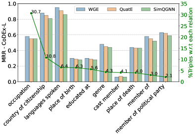
(a) Tail prediction on CoDEx-L.

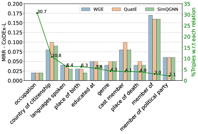
(b) Head prediction on CoDEx-L.

Figure 4: MRR on the CoDEx-L validation set w.r.t each relation. The right y-axis is the percentage of triples corresponding to each relation.

4.2.2 Qualitative study 

We report the performances of WGE, QuatE and SimQGNN over different relation types on the CoDEx validation sets in Figures 3 and 4. For each dataset, we select the top 10 frequent relations and compare model performances over these 10 relations. We also separate the result into tail prediction (i.e., predicting the tail entity given $(h,r,?)$) and head prediction (i.e., predicting the head entity given $(?,r,t)$). WGE generally works better than both QuatE and SimQGNN except for some special relation cases. For example, QuatE achieves higher head prediction scores for the relation “country of citizenship” than WGE as shown in Figures 3(b), 3(d) and 4(b). A possible reason is that some useful RF constraints related to the relation “country of citizenship” have been omitted from the relation-focused graph construction. Note that there is a substantial performance gap between the head prediction and the tail prediction, wherein predicting the tail entities is easier than predicting the head entities. The reason might come from the fact that in the CoDEx datasets, each relation is associated with a small number of tail entities but with a large number of head entities. For example, head entity candidates for “occupation” relations can be any person nodes, while candidates for tail entities are limited by the number of job entities.

4.3 Ablation analysis

Tables 3 and 4 present our ablation results on the validation sets for five variants of our proposed WGE, including:

• (1) A variant without predicate entities: This is a variant that only keeps relation nodes in the relation-focused view, i.e., without using the predicate entities as nodes from the extracted RF constraints.

• (2) A variant with GCN: This is a variant that uses GCN in the encoder module instead of using QGNN.

• (3) A variant with only entity-focused view: This is a variant that uses only the entity-focused view.

• (4) A variant with only relation-focused view: This is a variant that uses only the relation-focused view.

• (5) A variant with the Levi graph transformation: This is a variant where a single Levi graph is used as the input of the encoder module. From the given KG, we investigate another strategy of constructing a single undirected graph, which can be considered as a direct extension of our entity-focused graph view with additional relation nodes, following the Levi graph transformation [19].

Table 3: Ablation results on CoDEx validation sets for five variants of our WGE. (1) A variant where the relation-focused view uses only relation nodes, without using the predicate entities. (2) A variant utilizes GCN in the encoder module instead of using QGNN. (3) A variant utilizes only the entity-focused view. (4) A variant utilizes only the relation-focused view. (5) A variant uses the Levi graph transformation, i.e. the entity-focused graph view with addition relation nodes.

Method	CoDEx-S		CoDEx-M		CoDEx-L
	MRR	H@10	MRR	H@10	MRR	H@10
WGE	0.469	67.9	0.339	48.4	0.320	44.1
(1) w/o predicate entities	0.448	67.1	0.328	47.1	0.312	43.1
(2) w/ GCN	0.441	66.5	0.322	47.0	0.306	43.0
(3) w/ only entity-focused	0.452	66.9	0.329	46.5	0.314	43.0
(4) w/ only relation-focused	0.455	66.9	0.323	46.7	0.305	42.9
(5) w/ only Levi graph	0.447	63.5	0.320	45.7	0.288	41.1

Table 4: Ablation results on LitWD and FB15K-237 validation sets for five variants of our WGE.

Method	LitWD1K		LitWD19K		LitWD48K		FB15K-237
	MRR	H@10	MRR	H@10	MRR	H@10	MRR	H@10
WGE	0.518	75.5	0.343	49.5	0.402	59.3	0.351	53.6
(1) w/o predicate entities	0.483	72.6	0.326	47.9	0.389	57.2	0.339	52.4
(2) w/ GCN	0.470	71.3	0.325	47.2	0.382	56.6	0.327	50.2
(3) w/ only entity-focused	0.497	73.3	0.336	48.1	0.397	58.4	0.341	52.5
(4) w/ only relation-focused	0.498	73.7	0.338	48.4	0.395	58.4	0.340	52.3
(5) w/ only Levi graph	0.484	72.8	0.331	48.2	0.387	56.9	0.336	50.8

We find that WGE outperforms all of its variants, thus showing that: from (1), the predicate entities can help to better infer the potential dependence between two neighborhood relations; from (2), GCNs are not as effective as QGNNs; and from (3), (4) and (5), the modeling of two-view graphs of KGs helps produce better scores than single-view modeling of KGs, confirming the effectiveness of our two-view WGE approach. In addition, variant (5) obtains lower scores than variant (3), also showing that the Levi graph transformation is not as effective as the entity-focused graph transformation.

5 Conclusion

In this paper, we have introduced WGE—an effective GNN-based KG embedding model—to enhance the entity neighborhood information with the potential dependence between two neighborhood relations. In particular, WGE constructs two views from the given KG, including a single undirected entity-focused graph and a single undirected relation-focused graph. Then WGE proposes a new encoder architecture to update entity and relation vector representations from these two graph views. After that, WGE employs a weighted score function to compute the triple scores for KG completion. Extensive experiments show that WGE outperforms other strong GNN-based baselines and KG embedding models on seven KG completion benchmark datasets. Our WGE implementation is publicly available at: https://github.com/vinhsuhi/WGE.

Appendix

The hyper-complex vector space has recently been considered on the Quaternion space [15] consisting of one real and three separate imaginary axes. It provides highly expressive computations through the Hamilton product compared to the Euclidean and complex vector spaces. We provide key notations and operations related to the Quaternion space required for our later development. Additional details can further be found in [25].

A quaternion $q\in\mathbb{H}$ is a hyper-complex number consisting of one real and three separate imaginary components [15] defined as:

$$q=q_{r}+q_{i}\boldsymbol{\mathsf{i}}+q_{j}\boldsymbol{\mathsf{j}}+q_{k}\boldsymbol{\mathsf{k}}$$ (20)

where $q_{r},q_{i},q_{j},q_{k}\in\mathbb{R}$, and $\boldsymbol{\mathsf{i}},\boldsymbol{\mathsf{j}},\boldsymbol{\mathsf{k}}$ are imaginary units that $\boldsymbol{\mathsf{i}}^{2}=\boldsymbol{\mathsf{j}}^{2}=\boldsymbol{\mathsf{k}}^{2}=\boldsymbol{\mathsf{i}}\boldsymbol{\mathsf{j}}\boldsymbol{\mathsf{k}}=-1$. The operations for the Quaternion algebra are defined as follows:

Addition. The addition of two quaternions $q$ and $p$ is defined as:

$$q+p=(q_{r}+p_{r})+(q_{i}+p_{i})\boldsymbol{\mathsf{i}}+(q_{j}+p_{j})\boldsymbol{\mathsf{j}}+(q_{k}+p_{k})\boldsymbol{\mathsf{k}}$$ (21)

Norm. The norm $\|q\|$ of a quaternion $q$ is computed as:

$$\|q\|=\sqrt{q_{r}^{2}+q_{i}^{2}+q_{j}^{2}+q_{k}^{2}}$$ (22)

And the normalized or unit quaternion $q^{\triangleleft}$ is defined as: $q^{\triangleleft}=\frac{q}{\|q\|}$

Scalar multiplication. The multiplication of a scalar $\lambda$ and $q$ is computed as follows:

$$\lambda q=\lambda q_{r}+\lambda q_{i}\boldsymbol{\mathsf{i}}+\lambda q_{j}\boldsymbol{\mathsf{j}}+\lambda q_{k}\boldsymbol{\mathsf{k}}$$ (23)

Conjugate. The conjugate $q^{\ast}$ of a quaternion $q$ is defined as:

$$q^{\ast}=q_{r}-q_{i}\boldsymbol{\mathsf{i}}-q_{j}\boldsymbol{\mathsf{j}}-q_{k}\boldsymbol{\mathsf{k}}$$ (24)

Hamilton product. The Hamilton product $\otimes$ (i.e., the quaternion multiplication) of two quaternions $q$ and $p$ is defined as:

$$q\otimes p = (q_{r}p_{r}-q_{i}p_{i}-q_{j}p_{j}-q_{k}p_{k})$$

$$+ (q_{i}p_{r}+q_{r}p_{i}-q_{k}p_{j}+q_{j}p_{k})\boldsymbol{\mathsf{i}}$$

$$+ (q_{j}p_{r}+q_{k}p_{i}+q_{r}p_{j}-q_{i}p_{k})\boldsymbol{\mathsf{j}}$$

$$+ (q_{k}p_{r}-q_{j}p_{i}+q_{i}p_{j}+q_{r}p_{k})\boldsymbol{\mathsf{k}}$$ (25)

We can express the Hamilton product of $q$ and $p$ in the following form:

$$q\otimes p=\begin{bmatrix}1\\ \boldsymbol{\mathsf{i}}\\ \boldsymbol{\mathsf{j}}\\ \boldsymbol{\mathsf{k}}\end{bmatrix}^{\top}\begin{bmatrix}q_{r}&-q_{i}&-q_{j}&-q_{k}\\ q_{i}&q_{r}&-q_{k}&q_{j}\\ q_{j}&q_{k}&q_{r}&-q_{i}\\ q_{k}&-q_{j}&q_{i}&q_{r}\end{bmatrix}\begin{bmatrix}p_{r}\\ p_{i}\\ p_{j}\\ p_{k}\end{bmatrix}$$ (26)

The Hamilton product of two quaternion vectors $\boldsymbol{q}$ and $\boldsymbol{p}\in\mathbb{H}^{n}$ is computed as:

$$\boldsymbol{q}\otimes\boldsymbol{p} = (\boldsymbol{q}_{r}\circ\boldsymbol{p}_{r}-\boldsymbol{q}_{i}\circ\boldsymbol{p}_{i}-\boldsymbol{q}_{j}\circ\boldsymbol{p}_{j}-\boldsymbol{q}_{k}\circ\boldsymbol{p}_{k})$$

$$+ (\boldsymbol{q}_{i}\circ\boldsymbol{p}_{r}+\boldsymbol{q}_{r}\circ\boldsymbol{p}_{i}-\boldsymbol{q}_{k}\circ\boldsymbol{p}_{j}+\boldsymbol{q}_{j}\circ\boldsymbol{p}_{k})\boldsymbol{\mathsf{i}}$$

$$+ (\boldsymbol{q}_{j}\circ\boldsymbol{p}_{r}+\boldsymbol{q}_{k}\circ\boldsymbol{p}_{i}+\boldsymbol{q}_{r}\circ\boldsymbol{p}_{j}-\boldsymbol{q}_{i}\circ\boldsymbol{p}_{k})\boldsymbol{\mathsf{j}}$$

$$+ (\boldsymbol{q}_{k}\circ\boldsymbol{p}_{r}-\boldsymbol{q}_{j}\circ\boldsymbol{p}_{i}+\boldsymbol{q}_{i}\circ\boldsymbol{p}_{j}+\boldsymbol{q}_{r}\circ\boldsymbol{p}_{k})\boldsymbol{\mathsf{k}}$$ (27)

where $\circ$ denotes the element-wise product. We note that the Hamilton product is not commutative, i.e., $q\otimes p\neq p\otimes q$.

We can derived a product of a quaternion matrix $\boldsymbol{W}\in\mathbb{H}^{m\times n}$ and a quaternion vector $\boldsymbol{p}\in\mathbb{H}^{n}$ from Equation 26 as follow:

$$\boldsymbol{W}\otimes\boldsymbol{p}=\begin{bmatrix}1\\ \boldsymbol{\mathsf{i}}\\ \boldsymbol{\mathsf{j}}\\ \boldsymbol{\mathsf{k}}\end{bmatrix}^{\top}\begin{bmatrix}\boldsymbol{W}_{r}&-\boldsymbol{W}_{i}&-\boldsymbol{W}_{j}&-\boldsymbol{W}_{k}\\ \boldsymbol{W}_{i}&\boldsymbol{W}_{r}&-\boldsymbol{W}_{k}&\boldsymbol{W}_{j}\\ \boldsymbol{W}_{j}&\boldsymbol{W}_{k}&\boldsymbol{W}_{r}&-\boldsymbol{W}_{i}\\ \boldsymbol{W}_{k}&-\boldsymbol{W}_{j}&\boldsymbol{W}_{i}&\boldsymbol{W}_{r}\end{bmatrix}\begin{bmatrix}\boldsymbol{p}_{r}\\ \boldsymbol{p}_{i}\\ \boldsymbol{p}_{j}\\ \boldsymbol{p}_{k}\end{bmatrix}$$ (28)

where $\boldsymbol{p}_{r}$, $\boldsymbol{p}_{i}$, $\boldsymbol{p}_{j}$, and $\boldsymbol{p}_{k}\in\mathbb{R}^{n}$ are real vectors; and $\boldsymbol{W}_{r}$, $\boldsymbol{W}_{i}$, $\boldsymbol{W}_{j}$, and $\boldsymbol{W}_{k}\in\mathbb{R}^{m\times n}$ are real matrices.

Quaternion-inner product. The quaternion-inner product $\bullet$ of two quaternion vectors $\boldsymbol{q}$ and $\boldsymbol{p}\in\mathbb{H}^{n}$ returns a scalar as:

$$\boldsymbol{q}\bullet\boldsymbol{p}=\boldsymbol{q}_{r}^{\textsf{T}}\boldsymbol{p}_{r}+\boldsymbol{q}_{i}^{\textsf{T}}\boldsymbol{p}_{i}+\boldsymbol{q}_{j}^{\textsf{T}}\boldsymbol{p}_{j}+\boldsymbol{q}_{k}^{\textsf{T}}\boldsymbol{p}_{k}$$ (29)

Quaternion element-wise product. We further define the element-wise product of two quaternions vector $\boldsymbol{q}$ and $\boldsymbol{p}\in\mathbb{H}^{n}$ as follow:

$$\boldsymbol{p}*\boldsymbol{q}=(\boldsymbol{q}_{r}\circ\boldsymbol{p}_{r})+(\boldsymbol{q}_{i}\circ\boldsymbol{p}_{i})\boldsymbol{\mathsf{i}}+(\boldsymbol{q}_{j}\circ\boldsymbol{p}_{j})\boldsymbol{\mathsf{j}}+(\boldsymbol{q}_{k}\circ\boldsymbol{p}_{k})\boldsymbol{\mathsf{k}}$$ (30)

References

- [1] Balažević, I., Allen, C., Hospedales, T.M.: TuckER: Tensor Factorization for Knowledge Graph Completion. In: EMNLP. pp. 5185–5194 (2019)
- [2] Berant, J., Chou, A., Frostig, R., Liang, P.: Semantic Parsing on Freebase from Question-Answer Pairs. In: EMNLP. pp. 1533–1544 (2013)
- [3] Bordes, A., Usunier, N., García-Durán, A., Weston, J., Yakhnenko, O.: Translating Embeddings for Modeling Multi-relational Data. In: NIPS. pp. 2787–2795 (2013)
- [4] Bordes, A., Weston, J., Collobert, R., Bengio, Y.: Learning Structured Embeddings of Knowledge Bases. In: AAAI. pp. 301–306 (2011)
- [5] Chen, X., Zhou, Z., Gao, M., Shi, D., Husen, M.N.: Knowledge representation combining quaternion path integration and depth-wise atrous circular convolution. In: UAI. pp. 336–345 (2022)
- [6] Demir, C., Ngomo, A.C.N.: Convolutional Complex Knowledge Graph Embeddings. In: ESWC. pp. 409–424 (2021)
- [7] Dettmers, T., Minervini, P., Stenetorp, P., Riedel, S.: Convolutional 2D Knowledge Graph Embeddings. In: AAAI. pp. 1811–1818 (2018)
- [8] Dutta, S., Weikum, G.: Cross-Document Co-Reference Resolution using Sample-Based Clustering with Knowledge Enrichment. Transactions of the ACL 3, 15–28 (2015)
- [9] Fader, A., Zettlemoyer, L., Etzioni, O.: Open Question Answering over Curated and Extracted Knowledge Bases. In: KDD. pp. 1156–1165 (2014)
- [10] Ferrucci, D.A.: Introduction to ”This is Watson”. IBM Journal of Research and Development 56(3), 235–249 (2012)
- [11] Gesese, G.A., Alam, M., Sack, H.: LiterallyWikidata - A Benchmark for Knowledge Graph Completion Using Literals. In: ISWC. pp. 511–527 (2021)
- [12] Glorot, X., Bengio, Y.: Understanding the difficulty of training deep feedforward neural networks. In: AISTATS. pp. 249–256 (2010)
- [13] Hamilton, W.L., Ying, R., Leskovec, J.: Inductive representation learning on large graphs. In: NeurIPS (2017)
- [14] Hamilton, W.L., Ying, R., Leskovec, J.: Representation Learning on Graphs: Methods and Applications. IEEE Data Engineering Bulletin 40(3), 52–74 (2018)
- [15] Hamilton, W.R.: On Quaternions; or on a new System of Imaginaries in Algebra. The London, Edinburgh, and Dublin Philosophical Magazine and Journal of Science 25(163), 10–13 (1844)
- [16] Kingma, D., Ba, J.: Adam: A Method for Stochastic Optimization. In: ICLR (2015)
- [17] Kipf, T.N., Welling, M.: Semi-supervised classification with graph convolutional networks. In: ICLR (2017)
- [18] Krishnamurthy, J., Mitchell, T.: Weakly Supervised Training of Semantic Parsers. In: EMNLP-CoNLL. pp. 754–765 (2012)
- [19] Levi, F.W.: Finite Geometrical Systems: Six Public Lectues Delivered in February, 1940, at the University of Calcutta. University of Calcutta (1942)
- [20] Nguyen, D.Q., Nguyen, D.Q., Nguyen, T.D., Phung, D.: Convolutional Neural Network-based Model for Knowledge Base Completion and Its Application to Search Personalization. Semantic Web 10(5), 947–960 (2019)
- [21] Nguyen, D.Q., Nguyen, T.D., Phung, D.: Quaternion graph neural networks. In: ACML (2021)
- [22] Nguyen, D.Q., Tong, V., Phung, D., Nguyen, D.Q.: Node Co-occurrence based Graph Neural Networks for Knowledge Graph Link Prediction. In: WSDM. pp. 1589–1592 (2022)
- [23] Nguyen, D.Q.: A survey of embedding models of entities and relationships for knowledge graph completion. In: TextGraphs. pp. 1–14 (2020)
- [24] Nickel, M., Rosasco, L., Poggio, T.: Holographic Embeddings of Knowledge Graphs. In: AAAI. pp. 1955–1961 (2016)
- [25] Parcollet, T., Morchid, M., Linarès, G.: A survey of quaternion neural networks. Artificial Intelligence Review 53, 2957––2982 (2020)
- [26] Paszke, A., Gross, S., Massa, F., et al.: Pytorch: An imperative style, high-performance deep learning library. In: NeurIPS. pp. 8024–8035 (2019)
- [27] Ponzetto, S.P., Strube, M.: Exploiting Semantic Role Labeling, WordNet and Wikipedia for Coreference Resolution. In: NAACL. pp. 192–199 (2006)
- [28] Safavi, T., Koutra, D.: CoDEx: A Comprehensive Knowledge Graph Completion Benchmark. In: EMNLP. pp. 8328–8350 (2020)
- [29] Scarselli, F., Gori, M., Tsoi, A.C., Hagenbuchner, M., Monfardini, G.: The graph neural network model. IEEE Transactions on Neural Networks 20(1), 61–80 (2009)
- [30] Schlichtkrull, M., Kipf, T., Bloem, P., Berg, R.v.d., Titov, I., Welling, M.: Modeling relational data with graph convolutional networks. In: ESWC. pp. 593–607 (2018)
- [31] Shang, C., Tang, Y., Huang, J., Bi, J., He, X., Zhou, B.: End-to-end structure-aware convolutional networks for knowledge base completion. In: AAAI. pp. 3060–3067 (2019)
- [32] Toutanova, K., Chen, D.: Observed Versus Latent Features for Knowledge Base and Text Inference. In: CVSC. pp. 57–66 (2015)
- [33] Trouillon, T., Welbl, J., Riedel, S., Gaussier, É., Bouchard, G.: Complex Embeddings for Simple Link Prediction. In: ICML. pp. 2071–2080 (2016)
- [34] Vashishth, S., Sanyal, S., Nitin, V., Talukdar, P.: Composition-based multi-relational graph convolutional networks. In: ICLR (2020)
- [35] Veličković, P., Cucurull, G., Casanova, A., Romero, A., Liò, P., Bengio, Y.: Graph attention networks. In: ICLR (2018)
- [36] Wu, Z., Pan, S., Chen, F., Long, G., Zhang, C., Yu, P.S.: A Comprehensive Survey on Graph Neural Networks. IEEE Transactions on Neural Networks and Learning Systems 32(1), 4–24 (2021)
- [37] Yang, B., Yih, W.t., He, X., Gao, J., Deng, L.: Embedding Entities and Relations for Learning and Inference in Knowledge Bases. In: ICLR (2015)
- [38] Zhang, D., Yin, J., Zhu, X., Zhang, C.: Network representation learning: A survey. IEEE Transactions on Big Data 6, 3–28 (2020)
- [39] Zhang, S., Tay, Y., Yao, L., Liu, Q.: Quaternion knowledge graph embeddings. In: NeurIPS. pp. 2731–2741 (2019)
- [40] Zhang, Y., Yao, Q., Dai, W., Chen, L.: AutoSF: Searching Scoring Functions for Knowledge Graph Embedding. In: ICDE. pp. 433–444 (2020)