Closely spaced co-rotating helical vortices: Long-wave instability

Abstract

We consider as base flow the stationary vortex filament solution obtained by Castillo-Castellanos et al. (2021) in the far-wake of a rotor with tip-splitting blades. The cases of a single blade and of two blades with a hub vortex are studied. In these solutions, each blade generates two closely spaced co-rotating tip vortices that form a braided helical pattern in the far-wake. The long-wave stability of these solutions is analysed using the same vortex filament framework. Both the linear spectrum and the linear impulse response are considered. We demonstrate the existence of different types of instability modes. A first type corresponds to the local pairing of consecutive turns of the helical pattern, which is well described by the instability of an uniform helical vortex with a core size given by the mean separation distance of the vortices in the pair. A second type corresponds to the pairing of consecutive turns of vortex pair and is observed only for densely braided patterns, which is well described by the instability of two interlaced helical vortices by straightening out the baseline helix. A third type of unstable modes modifies the separation distance between the vortices in each pair and amplifies specific (linear) wavelengths. These unstable modes also spread spatially with a weaker rate.

1 Introduction

Rotating blades, such as those of a helicopter rotor or a horizontal-axis wind turbine, generate concentrated vortices at their tips, transported downstream, creating a distinctive helical pattern. These helical vortices are associated with several practical issues actively investigated. One of these issues is the wake stability with respect to external disturbances, which has practical relevance since instabilities may accelerate the vortex break-up and the transition towards turbulent wakes. The interaction between tip vortices and a solid surface, like a trailing rotor blade, or a wind turbine located downstream, may cause significant noise, vibration, and fatigue problems. Wake stability is also fundamental to optimize wind farms design, since wakes may extend up to 50 km downstream under stable atmospheric conditions (Cañadillas et al., 2020). Strategies to maximize power generation include dynamically varying the yaw, pitch, and tip-speed ratio to excite the natural instability of helical wakes (see, for instance Huang et al. (2019); Frederik et al. (2020); Brown et al. (2022)).

One alternative to accelerate the vortex breakdown is to modify the wake structure altogether. Brocklehurst & Pike (1994) introduced a modified vane tip to split the tip vortex into two co-rotating vortices. The associated spreading of vorticity has been suggested as indicative of reduced noise and increased aerodynamic efficiency, but there is little information regarding the change in the wake structure, which is essential to optimize the air-foil design. The present work aims to fill in some of these gaps by focusing on the instabilities of closely-spaced helical vortices. A recent experimental investigation of two closely spaced helical vortices generated by single-bladed rotor, Schröder et al. (2020, 2021) displays a rapid increase of the core radii and subsequent merging related to the development of a centrifugal instability (Bayly, 1988). In this case, the centrifugal instability is triggered by patches of opposite signed vorticity formed by a protruded fin during the roll-up process. A theoretical analysis by Castillo-Castellanos et al. (2021) presented the wake geometry produced by a tip-splitting rotor for all wind turbine and helicopter flight regimes using a filament approach. The resulting wake deviates from a helical pattern in favour of an epicycloidal pattern produced by two interlaced helical vortices inscribed on top of a larger helical curve. From afar, the vortex structure is reminiscent of a helical vortex, while simultaneously resembling a vortex pair aligned with the locally tangent flow. Given these similarities, we expect the solutions to display features from both systems. In particular, similar instability mechanisms.

Studies on the stability of helical vortices started a century ago (see for instance Levy & Forsdyke, 1928) although experimental evidence of short-wave and long wave instabilities are quite recent (Leweke et al., 2014). Theoretical predictions for the long-wave instability have been obtained by Widnall (1972) for a uniform helical vortex. Her work was extended by Gupta & Loewy (1974) for several helices and by Fukumoto & Miyazaki (1991) to account the effect of an axial flow within the vortices. As demonstrated by Quaranta et al. (2015, 2019), the long-wave instability is a local pairing instability (Lamb, 1945). The instability modes are associated with a displacement approaching neighbouring loops at specific locations. Quaranta et al. (2019) have also shown that their growth rate is well-predicted by considering 3D perturbations on straight vortices (Robinson & Saffman, 1982). For several helices, additional theoretical results have been obtained for the global pairing mode which preserves the helical symmetry of the flow (Okulov, 2004; Okulov & Sørensen, 2007) using Hardin’s expressions for the induced velocity of a helical vortex (Kawada, 1936; Hardin, 1982). This mode has been further analysed in the non-linear regime by Selçuk et al. (2017). Finally, recent numerical works have also evidenced the presence of the long-wave instability in the context of rotor-generated vortices (Bhagwat & Leishman, 2000; Walther et al., 2007; Ivanell et al., 2010; Durán Venegas et al., 2021). Helical vortices are also unstable to short-wavelength instabilities, due to the modification of the core structure by curvature, torsion and strain (Kerswell, 2002; Blanco-Rodríguez & Le Dizès, 2016, 2017). This requires detailed information of the inner core structure, which can be obtained through matched asymptotic techniques (Blanco-Rodríguez et al., 2015), or through direct numerical simulations (Selçuk et al., 2017; Brynjell-Rahkola & Henningson, 2020). Pairs display a variety of complex behaviors (Leweke et al., 2016). For instance, consider a vortex pair of circulations $\Gamma_{1}$ and $\Gamma_{2}$ and core radii $a$, separated by a distance $d$. If $d$ is large enough, the system is expected to translate with constant speed for $\Gamma_{1}=-\Gamma_{2}$, or rotate around the vorticity barycentre with constant rotation rate for all other cases, while $a$ is expected to grow following a viscous law. Pairs are expected to merge as a critical core size is eventually reached (Meunier et al., 2002; Josserand & Rossi, 2007). This behaviour is modified by the development of short-wave instabilities (Meunier & Leweke, 2005) and long-wave instabilities (Crow, 1970; Jimenez, 1975). This picture becomes increasingly complex as we consider the interactions between multiple vortex pairs, like the four vortex system considered by (Crouch, 1997; Fabre & Jacquin, 2000; Fabre et al., 2002).

For this work, we focus on the long-wavelength stability of two closely-spaced helical vortices using a filament approach. This approach has the advantage of filtering the short-wavelength perturbations. Additionally, we are interested in the regime observed in the far-field, since perturbations are expected to be quickly advected away from the rotor (Durán Venegas et al., 2021). We shall use as base flow the steady solutions obtained in Castillo-Castellanos et al. (2021). Depending on the geometric parameters, these solutions are classified as (i) leapfrogging, (ii) sparsely braided, and (iii) densely braided wakes. From afar, the periodic structure is reminiscent of a helical vortex but up close, it resembles two interlaced helical vortices aligned with the locally tangent flow. Given these similarities, we expect he stability of the present system to be understood as a combination of the pairing modes of

• a helical vortex of radius $R$, pitch $H$, circulation $2\Gamma$, and some effective core size $a_{e}$

• a pair of helical vortices of radius $d/2$, pitch $h_{\tau}$, core size $a$, and circulation $\Gamma$

and by the possible interactions between them. We shall see that both kinds of pairing are observed, as well as a new kind of unstable modes specific to this configuration.

The paper is organized as follows. In section 2 we present the framework of the vortex method applied to the pair of helical vortices. We describe the numerical procedures to obtain the base flow and analyse its stability. In section 3, we apply our numerical approach to uniform helices for validation. We then consider two different configurations. The stability properties for a pair of helical vortices without a central vortex hub are presented in section 4 for the different wake geometries, while the stability properties for two pairs of helical vortices with a central hub vortex are presented in section 5 for leapfrogging wakes. In both cases, the structure of the unstable modes is presented in detail and we explore the influence of the main geometric parameters. Additional information regarding the spatio-temporal development of the instability is provided in the appendix A, where the linear impulse response for the first configuration is studied using the approach developed by Durán Venegas et al. (2021). Finally, we present our main conclusions in section 6.

2 Methodology

2.1 Finding stationary solutions using a filament approach

2.1.1 Filament framework

We use the same vortex filament approach as in Durán Venegas & Le Dizès (2019). Vorticity is considered to be concentrated along slender vortex filaments moving as material lines in the fluid according to

$$\frac{{\rm d}\boldsymbol{X}_{j}}{{\rm d}t}=\boldsymbol{U}(\boldsymbol{X}_{j})-{U}_{z}^{\infty}\boldsymbol{\hat{e}_{z}}$$ (1)

where $\boldsymbol{X}_{j}=(r_{j},\theta_{j},z_{j})$ is the position of the $j$-th vortex filament, ${U}_{z}^{\infty}$ an external velocity field, and $\boldsymbol{U}(\boldsymbol{X}_{j})=(U_{r},r_{j}\Omega,U_{z})$ is the velocity induced by the vortices at $\boldsymbol{X}_{j}$. In a frame with rotation rate $\Omega_{R}$, it is convenient to parametrize the position of vortex filaments in terms of two angular coordinates, $\zeta=\Omega_{R}(t-t_{0})$ and $\psi=\Omega_{R}t$, and transform (1) as

$$\frac{\partial\boldsymbol{X}_{j}}{\partial\psi}+\frac{\partial\boldsymbol{X}_{j}}{\partial\zeta}=\frac{1}{\Omega_{R}}\left[\boldsymbol{U}(\boldsymbol{X}_{j})+\boldsymbol{U}^{\infty}(\boldsymbol{X}_{j})\right]$$ (2)

where $\boldsymbol{U}^{\infty}(\boldsymbol{X}_{j})=(0,-r_{j}\Omega_{R},-{U}_{z}^{\infty})$ contains the contributions from the rotating frame and a constant free-stream velocity. In this context, $\zeta$ is often referred to as the wake age and corresponds to a spatial coordinate, while $\psi$ is a proxy of time (Leishman et al., 2002). Filaments are discretized in straight segments $[\boldsymbol{X}^{n}_{j},\boldsymbol{X}^{n+1}_{j}]$ in order to compute the velocity field using the Biot-Savart law. The equation is de-singularized using a cut-off approach with a Gaussian vorticity profile. Local contributions to the velocity field at $\boldsymbol{X}_{j}^{n}$ are obtained by replacing the straight segments by an arc of circle passing through $[\boldsymbol{X}^{n-1}_{j},\boldsymbol{X}^{n}_{j},\boldsymbol{X}^{n+1}_{j}]$ and use the cut-off formula (see, Durán Venegas & Le Dizès (2019)).

For this work, we consider basic flow solutions that satisfy,

$$\frac{{\rm d}r_{j}}{{\rm d}\zeta}=\frac{U_{r}(\boldsymbol{X}_{j})}{\Omega_{R}},\quad\frac{{\rm d}\theta_{j}}{{\rm d}\zeta}=\frac{\Omega(\boldsymbol{X}_{j})-\Omega_{R}}{\Omega_{R}},\quad\frac{{\rm d}z_{j}}{{\rm d}\zeta}=\frac{U_{z}(\boldsymbol{X}_{j})-U^{\infty}_{z}}{\Omega_{R}}.$$ (3)

These solutions are $\psi$-independent solutions to (2). They are stationary in the moving frame in the sense that flow remains tangent to the vortex structure at all times:

$$(\boldsymbol{U}(\boldsymbol{X}_{j})+\boldsymbol{U}^{\infty}(\boldsymbol{X}_{j}))\times\boldsymbol{T}_{j}=0$$ (4)

where $\boldsymbol{T}_{j}$ is the tangent unit vector. As shown in Castillo-Castellanos et al. (2021), the spatial evolution of the wake as we move away from the rotor plane is obtained by numerically solving (3) with boundary conditions on the rotor, at $\zeta=0$, where the position of each vortex is prescribed and far-field boundary conditions at $\zeta\to\infty$. In the following, we focus on the wake geometry in the far-field, where spatially periodic solutions are obtained.

2.1.2 Periodic solutions in the far-field

The solution in the far-field has been obtained in Castillo-Castellanos et al. (2021). It was shown that it is no longer uniform as for a single helix but it nevertheless exhibits a certain spatial periodicity. In addition to the azimuthal symmetry $\theta\to\theta+2\pi/N$ for $N$ vortex pairs, solutions are invariant by the double operation $z\to z+h$ and $\theta\to\theta+2\pi/\beta$. The parameters $h$ and $\beta$ are chosen such that there is a single location in an axial period $h$ where the vortices of a given pair are at the same azimuth. This azimuth is taken to define the mean radius $R$ and the separation distance $d$ of each vortex pair. Each vortex pair tends to form a helical braid on a larger helical structure of radius $R$ and pitch $H$ as illustrated on figure 1.

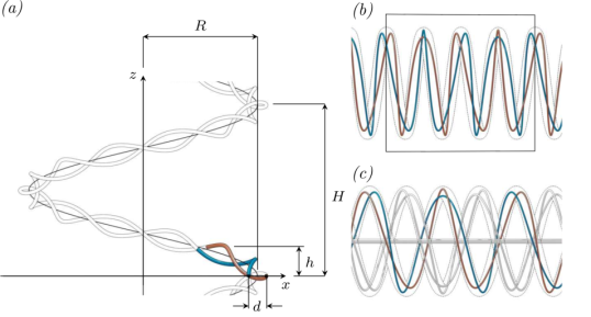
Figure 1: (a) Geometric parameters of periodic solutions: separation distance $d$, radius $R$, axial pitches $H$ and $h$, core size $a$ and $\beta=H/h$. Representation of (b) $N=1$ pairs without hub vortex and (c) $N=2$ pairs with hub vortex for ($R^{*}=7$, $H^{*}/N=5.25$, $\beta=3/4$).

The pitch of this larger helical structure is directly related to $h$ and $\beta$ by

$$H=h\beta$$ (5)

and related to the pitch of the vortex pair through

$$h_{\tau}=\sqrt{H^{2}+(2\pi R)^{2}}/\beta.$$ (6)

Depending on the value of $\beta$, the double-helix structure may describe (i) a leapfrog-type pattern, where vortices trade places every $1/\beta$ turns; (ii) a relatively sparse braid ; or (iii) a dense ‘telephone cord’-type pattern. We are typically in situation (i) when $\beta<1$, and in situation (iii) when $\beta>10$. The parameter $\beta$ also characterizes the axial periodicity of the solution. It becomes axially periodic only if $\beta$ is a rational number $p/q$. In that case, it means that the double helix makes $q$ turns on itself as the large helix does $p$ turns. The axial period is thus $pH=qh$. In the following, we only consider rational values of $\beta$.

As soon as the vortex core size $a$ is fixed, the far-field is then defined by 5 non-dimensional parameters which are

$$R^{*}\equiv\frac{R}{d},\quad H^{*}\equiv\frac{H}{d},\quad\varepsilon^{*}\equiv\frac{a}{d},\quad\beta,\quad N.$$ (7)

The solution is obtained by solving the system (3) with the prescribed symmetry. The frame velocities $(\Omega_{R},U^{\infty}_{z})$ are unknown quantities. However, these quantities are proportional to the vortex circulation $\Gamma$ as it is the unique quantity of the vortex system involving time. For this reason, we can fix $\Gamma$ to 1.

As shown in Castillo-Castellanos et al. (2021), the problem can be treated as a non-linear minimization problem using an iterative procedure. The convergence is rapid if we start for each pair from an initial guess given by an undeformed double helix on a larger helix and estimates for $(\Omega_{R},U^{\infty}_{z})$ obtained from uniform helices. The converged solution is found to exhibit spatial variations but in most cases the initial guess turns out to be a good approximation of the solution.

In the present study, we consider two different configurations: one composed of a single helical pair ($N=1$) without central hub vortex (figure 1b), and another composed of $N=2$ helical pairs with a central hub vortex (figure 1c). Also, we fix $\varepsilon^{*}=0.1$ and vary the remaining parameters ($R^{*}$, $H^{*}$ and $\beta$). In the following, solutions that satisfy (3) are denoted $\boldsymbol{X}_{j}^{B}(\zeta)$.

2.2 Inviscid global instability analysis

The stability of $\boldsymbol{X}_{j}^{B}$ is analysed by considering the evolution of infinitesimal perturbation displacements

$$\boldsymbol{X}_{j}(\zeta,\psi)=\boldsymbol{X}_{j}^{B}(\zeta)+\boldsymbol{X}^{\prime}_{j}(\zeta,\psi)$$ (8)

Equation (2) is linearized around $\boldsymbol{X}_{j}^{B}(\zeta)$ to obtain a linear dynamical system

$$\frac{\partial r_{i}^{\prime}}{\partial\psi} = -\frac{\partial r_{i}^{\prime}}{\partial\zeta}+\frac{1}{\Omega_{R}}\sum_{j=1}^{N}\left[\frac{\partial U_{r}(\vec{X}_{i}^{B})}{\partial r_{j}}r_{j}^{\prime}+\frac{\partial U_{r}(\vec{X}_{i}^{B})}{\partial\theta_{j}}\theta^{\prime}_{j}+\frac{\partial U_{r}(\vec{X}_{i}^{B})}{\partial z_{j}}z^{\prime}_{j}\right]$$ (9a)

$$\frac{\partial\theta_{i}^{\prime}}{\partial\psi} = -\frac{\partial\theta_{i}^{\prime}}{\partial\zeta}+\frac{1}{\Omega_{R}}\sum_{j=1}^{N}\left[\frac{\partial\Omega(\vec{X}_{i}^{B})}{\partial r_{j}}r_{j}^{\prime}+\frac{\partial\Omega(\vec{X}_{i}^{B})}{\partial\theta_{j}}\theta^{\prime}_{j}+\frac{\partial\Omega(\vec{X}_{i}^{B})}{\partial z_{j}}z^{\prime}_{j}\right]$$ (9b)

$$\frac{\partial z_{i}^{\prime}}{\partial\psi} = -\frac{\partial z_{i}^{\prime}}{\partial\zeta}+\frac{1}{\Omega_{R}}\sum_{j=1}^{N}\left[\frac{\partial U_{z}(\vec{X}_{i}^{B})}{\partial r_{j}}r_{j}^{\prime}+\frac{\partial U_{z}(\vec{X}_{i}^{B})}{\partial\theta_{j}}\theta^{\prime}_{j}+\frac{\partial U_{z}(\vec{X}_{i}^{B})}{\partial z_{j}}z^{\prime}_{j}\right]$$ (9c)

which has the following general form

$$\frac{\partial\boldsymbol{q}^{\prime}}{\partial\psi}=\mathsfbi{L}(\zeta)\boldsymbol{q}^{\prime}(\zeta,\psi)$$ (10)

where $\boldsymbol{q}^{\prime}=(\boldsymbol{X}_{1},\boldsymbol{X}_{2},\cdots)$ is the total displacement vector, and $\mathsfbi{L}$ is a $N$ by $N$ block-matrix containing the Jacobian terms. The spatial derivative (on $\zeta$) is evaluated using the same finite differences scheme as the base solution, while the velocity gradient is derived from the discretized Biot-Savart equations.

Each sub-matrix of $\mathsfbi{L}$ can be written as

$$\mathsfbi{L}_{ij}=-\delta_{ij}\frac{\partial}{\partial\zeta}+\frac{1}{\Omega_{R}}\frac{\partial(\boldsymbol{U}(\boldsymbol{X}_{i}^{B}))}{\partial(\boldsymbol{X}_{j})}$$ (11)

and contains $3n_{s}$ by $3n_{s}$ elements where $n_{s}$ is the total number of discretization point of each vortex. The base flow is periodic with respect to $\zeta$ with a period $\zeta_{B}$ that satisfies $z_{j}(\zeta_{B})=h$ and $\theta_{j}(\zeta_{B})=2\pi/\beta$. The difference between $\zeta_{B}$ and $\theta_{j}(\zeta_{B})$ comes from the induced angular velocity $\Omega(\boldsymbol{X}_{j})$ in (3)b. For small values of $\beta$, the ratio $C_{\theta}\equiv\zeta_{B}/\theta_{j}(\zeta_{B})$ is close to 1, but decreases as $\beta$ increases (figures 2a and 2b). Each vortex contains 96 points per period $\zeta_{B}$. For the perturbations we consider a longer domain with a period $\zeta_{p}=n_{p}\zeta_{B}$ with $n_{p}=32\beta$ such that $z_{j}(\zeta_{p})=n_{p}h=32H$ and $\theta_{j}(\zeta_{p})=n_{p}2\pi/\beta=64\pi$. This gives $n_{p}=24$ and $n_{p}=256$ for the values $\beta=3/4$ and $\beta=8$. For densely braided wakes ($\beta>20$), we use a shorter domain with $n_{p}=4\beta$, such that $z_{j}(\zeta_{p})=n_{p}h=4H$ and $\theta_{j}(\zeta_{p})=n_{p}2\pi/\beta=8\pi$. This gives $n_{p}=84$ and $n_{p}=128$ for the values $\beta=21$ and $\beta=32$. Our objective is to apply periodic boundary conditions to the perturbations. We therefore discretize the operators $\mathsfbi{L}_{ij}$ such that they satisfy this property.

(a) (b)  

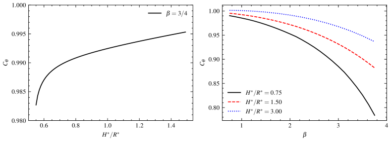
Figure 2: Evolution of the ratio $C_{\theta}\equiv\zeta_{B}/\theta_{j}(\zeta_{B})$ for ($N=1$, $R^{*}=7$): (a) $C_{\theta}$ as function $H^{*}/R^{*}$ for $\beta=3/4$, and (b) as function of $\beta$ for different $H^{*}/R^{*}$.

The final problem reduces to a linear system with constant coefficients that admits the formal solution

$$\boldsymbol{q}^{\prime}(\zeta,\psi)=\exp(\mathsfbi{L}\psi)\boldsymbol{q}_{0}^{\prime}(\zeta)$$ (12)

for any initial perturbation $\boldsymbol{q}^{\prime}_{0}(\zeta)=\boldsymbol{q}^{\prime}(\zeta,0)$. In standard fashion, treating equation (12) as an eigenvalue problem can be used to describe the asymptotic limit $\psi\to\infty$. Here, because the domain is long but periodic, it also means that we consider perturbations that span the whole calculation domain.

We may decompose the linear operator as

$$\mathsfbi{L}\mathsfbi{\Phi}=\mathsfbi{\Phi}\mathsfbi{\Lambda}$$ (13)

where $\mathsfbi{\Phi}$ is a matrix whose columns $(\boldsymbol{\phi}_{1},\boldsymbol{\phi}_{2},\cdots)$ are the eigenvectors of $\mathsfbi{L}$, and $\mathsfbi{\Lambda}$ is a matrix whose diagonal entries are the corresponding (complex) eigenvalues $(\lambda_{1},\lambda_{2},\cdots)$. Here, $\sigma_{m}\equiv\Real(\lambda_{m})$ characterizes the temporal growth (or decay) of the perturbations, while $\omega_{m}\equiv\Imag(\lambda_{m})$ characterizes the temporal oscillations. We may also introduce a dimensionless growth rate $\sigma_{m}^{*}$ and frequency $\omega_{m}^{*}$, based on the characteristic advection time-scale of helical pairs $t_{adv}=\Gamma/(H^{2}/N^{2})$. Since $\mathsfbi{L}$ is real-valued, modes are either real or come in conjugate pairs. Equation (12) can be written as

$$\boldsymbol{q}^{\prime}(\zeta,\psi)=\sum_{m}\boldsymbol{\phi}_{m}(\zeta)\exp{\{\sigma_{m}\psi+i\omega_{m}\psi\}}b_{m}+c.c.$$ (14)

where the coefficients $b_{m}$ correspond to the coordinates of $\boldsymbol{q}^{\prime}_{0}(\zeta)=\boldsymbol{q}^{\prime}(\zeta,0)$ expressed in the eigenvector basis, and $c.c.$ indicates the complex conjugate.

By construction, eigenvectors have the same dimensionality as $\boldsymbol{q^{\prime}}$,

$$\boldsymbol{\phi}_{m}=(\boldsymbol{\phi}_{m}^{(1)},\boldsymbol{\phi}_{m}^{(2)},\cdots)$$ (15)

where $\boldsymbol{\phi}_{m}^{(j)}$ is the $m$-th eigenvector of the $j$-th vortex filament. These eigenvectors represent a displacement vector and can be expressed in any coordinate system, e.g.,

$$\boldsymbol{\phi}_{m}^{(j)}=(\check{r}_{m}^{(j)},\check{\theta}_{m}^{(j)},\check{z}_{m}^{(j)})$$ (16)

indicates the components of $\boldsymbol{\phi}_{m}^{(j)}$ in global cylindrical coordinates. Conversely, displacement perturbations may also be expressed in terms of the local radial, azimuthal, and axial coordinates associated with a uniform helix $\mathscr{H}$ of radius $R$ and pitch $H$,

$$\boldsymbol{\phi}_{m}^{(j)}=(\check{\rho}_{m}^{(j)},\check{\phi}_{m}^{(j)},\check{s}_{m}^{(j)}).$$ (17)

Due to the spatial periodicity, the eigenvectors can be expanded on a discrete Fourier basis:

$$\boldsymbol{\phi}_{m}=\sum_{n=0}^{n_{s}-1}\boldsymbol{\hat{q}}_{mn}\exp{\left\{\frac{\mathrm{i}2\pi n\zeta}{\zeta_{p}}\right\}}$$ (18)

where the azimuthal wavenumber $(k=n\Delta k,\Delta k=\beta/n_{p})$ is normalized to ensure that $k=1$ corresponds to one helix turn, and $n_{s}$ the number of points used to discretize each vortex.

3 Validation of the stability analysis: uniform helices

We validate our approach against existing results on uniform helical vortices of pitch $H$, radius $R$ and effective core size $a_{e}$. A notable difference with respect to Widnall (1972) is that we must specify a reference frame with rotation rate $\Omega_{R}$ such that (3) is satisfied. Since the motion of helical vortices is described by constant rotation rate $\Omega$ and axial velocity $U_{z}$, these vortices are unperturbed by an additional rotation of angular velocity $\Omega^{a}$ and translation of axial velocity $U_{z}^{a}$ provided that

$$\frac{U_{z}^{a}}{\Omega^{a}}=\pm\frac{H}{2\pi}$$ (19)

is satisfied, where the sign is positive for right-handed helices and vice versa. For this comparison, we consider a rotating frame of reference

$$\Omega_{R}=\Omega\mp U_{z}\frac{2\pi}{H},\quad\quad U_{z}^{\infty}=0$$ (20)

which is commonly used in numerical simulations.

(a) (b)  

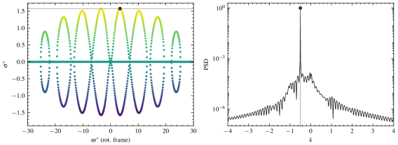
(c) (d)  

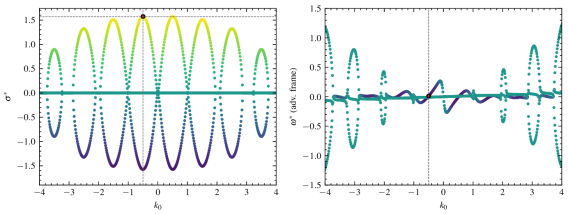
Figure 3: Stability of a uniform helix for $H/R=\pi/5$ and $a_{e}/R=0.1$: (a) $\sigma^{*}$ as function of $\omega^{*}$ in the rotating frame; (b) Fourier spectra of the mode indicated as a red mark in (a); (c) $\sigma^{*}$ and (d) $\omega^{*}$ in the advection frame as function of dominant wavenumber $k_{0}$.

	$a_{e}/R=0.10$			$a_{e}/R=0.20$			$a_{e}/R=0.33$
	1 Peak	2 Peak	3 Peak	1 Peak	2 Peak	3 Peak	1 Peak	2 Peak	3 Peak
$\sigma^{*}$	1.575	1.511	1.323	1.554	1.497	1.381	1.538	1.485	1.395
$\omega^{*}$	3.405	10.202	16.980	3.186	9.639	15.985	3.028	9.160	15.190
$k_{0}$	-0.500	-1.500	-2.500	-0.500	-1.516	-2.516	-0.500	-1.516	-2.516
$c_{0}$	1.006	1.004	1.003	1.005	1.003	1.001	1.004	1.002	1.001

Table 1: Growth rate, frequency, wavenumber and phase velocity for the most unstable modes of a uniform helix for $H/R=\pi/5$ and different core sizes. Here, $\Delta k=0.01625$.

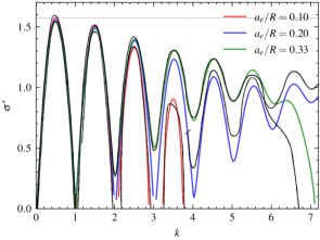
Figure 4: Dimensionless growth rate $\sigma^{*}$ of a uniform helix as function of $k_{0}$ for $H/R=\pi/5$ and different core sizes. Black thin lines correspond to figure 5d reproduced from Widnall (1972), while colour lines correspond to our numerical approach.

The (temporal) frequency spectra for a helix of pitch $H/R=\pi/5$ and $a_{e}/R=0.1$ is presented in figure 3a. By construction, the spectrum is symmetric with respect to zero, i.e. $\sigma^{*}(\omega^{*})=\sigma^{*}(-\omega^{*})$, and only the positive frequencies are displayed. The most unstable frequencies are located near $\omega^{*}=3$ with additional local maxima at odd multiples of this frequency (see left panel in table 1). Figure 3b displays the Fourier spectrum of $\check{z}_{m}$ for the most unstable mode, which is characterized by a single peak at $k=-0.500$. We can show that each eigenvector has the form of a complex wave with a single dominant wavenumber $k=k_{0}$, such that a direct correspondence between $\sigma_{m}$, $\omega_{m}$ and $k$ can be established, see figure 3c.

Axial perturbations propagate along the structure as the sum of travelling waves

$$z^{\prime}(\zeta,\psi)=\sum_{m}\hat{z}_{m}\cos(\omega_{m}\psi+k_{0}\zeta/C_{\theta})e^{\sigma_{m}\psi}$$ (21)

with phase velocity

$$c_{0}=-\omega_{m}C_{\theta}/k_{0}.$$ (22)

A similar behaviour is observed for radial and azimuthal perturbations. As noted by Brynjell-Rahkola & Henningson (2020), the frequencies obtained in a frame rotating with $\Omega_{R}$ can be mapped into a second reference frame rotating with $\Omega_{R}^{\prime}$ through

$$\omega_{m}^{\prime}=\omega_{m}+(\Omega_{R}^{\prime}-\Omega_{R})k/C_{\theta}.$$ (23)

For instance, in our example most of the tangential velocity comes from the moving frame, i.e., $|\Omega|\ll|\Omega-\Omega_{R}|$, such that perturbations are advected with $c_{0}$ close to 1, see table 1. If, instead, we consider a frame moving with the vortex elements, perturbations are advected with $c_{0}$ close to 0 for the same wavenumber (figure 3d).

As seen in figure 4, our numerical results are in good agreement with the stability curves presented in figure 5d by Widnall (1972) and figure 3 by Quaranta et al. (2015) for the same parameters. As mentioned in section 2.2, our approach differs from previous works in the way the Jacobian matrix is evaluated. As long as the base flow is (spatially) periodic, it is allowed to take any shape since equation (9) is evaluated directly from the discretised vortex segments. This will be useful for studying the more geometrically challenging helical pairs.

4 Stability of one vortex pair without central hub vortex

In this section, we describe the unstable modes for the case of one vortex pair without central hub vortex. Depending on the geometric parameters, some modes become more prominent than others. For clarity, we introduce progressively the unstable modes for (i) leapfrogging, (ii) sparsely braided and (iii) densely braided wakes. Leapfrogging wakes display two types of unstable modes: the pairing of the large-scale pattern and a new type specific to this configuration. Sparsely braided wakes display an additional type, which becomes more prominent as $\beta$ increases. Finally, densely braided wakes display an additional type, which corresponds to the pairing modes of the vortex pair.

4.1 Typical displacement modes for leapfrogging wakes

For each pair, we introduce the following decomposition

$$\boldsymbol{X}_{+}\equiv(\boldsymbol{X}_{1}+\boldsymbol{X}_{2})/2,\quad\quad\boldsymbol{X}_{-}\equiv(\boldsymbol{X}_{1}-\boldsymbol{X}_{2})/2$$ (24)

where $\boldsymbol{X}_{+}$ characterises the large-scale pattern traced by the vorticity barycentre, while $\boldsymbol{X}_{-}$ represents the rotation of the vortex pair relative to $\boldsymbol{X}_{+}$. Figure 1b depicts a leapfrogging wake with $\beta=p/q=3/4$, where $\boldsymbol{X}_{+}$ is represented as a tube enclosing the vortex pair. Over a single period, the vortex pair completes $p=3$ rotations around $\mathscr{H}$, while $\mathscr{H}$ completes $q=4$ rotations around the $z$ axis. Note that $\boldsymbol{X}_{+}$ and $\mathscr{H}$ are close but not exactly equal due to the effect of self-induction. In a similar vein, we introduce the following decomposition

$$\boldsymbol{\phi}_{m}^{+}\equiv(\boldsymbol{\phi}_{m}^{(1)}+\boldsymbol{\phi}_{m}^{(2)})/2,\quad\quad\boldsymbol{\phi}_{m}^{-}\equiv(\boldsymbol{\phi}_{m}^{(1)}-\boldsymbol{\phi}_{m}^{(2)})/2$$ (25)

where $\boldsymbol{\phi}_{m}^{+}$ and $\boldsymbol{\phi}_{m}^{-}$ indicate the displacement modes of $\boldsymbol{X}_{+}$ and $\boldsymbol{X}_{-}$, respectively.

Figure 5 presents the frequency spectrum, which is characterized by a set of modes distributed over three contiguous lobes at low frequencies, and a second set of modes over an additional lobe at higher frequencies. The maximum growth rate is observed near $\omega^{*}=4.8$, with additional local maxima (in descending order) near $\omega^{*}=51.9$, $\omega^{*}=14.5$, and $\omega^{*}=24.0$. These values respectively correspond to dominant wavenumbers $k_{0}=0.5$, $k_{0}=5.4$, $k_{0}=1.5$, and $k_{0}=2.5$. Dimensionless growth rates are slightly larger than the equivalent helical vortex (figure 5b). This can be explained by the change in the effective distance separating neighbouring loops.

Low frequency modes are clearly reminiscent of the unstable modes for the equivalent uniform helices, while those at higher frequencies are specific to this geometry. The two groups differ in the relative alignment between the displacements of the pair: predominantly aligned displacements (or symmetric with respect to the vorticity barycentre, figure 5c top) for low frequency modes and predominantly opposed displacements (or anti-symmetric with respect to the vorticity barycentre, figure 5c bottom) for those at higher frequencies. A more quantitative way to illustrate this difference is through the spatial cross-correlation

$$(z_{i}^{\prime}\star z_{j}^{\prime})(\Delta\theta)\equiv\int_{\infty}^{\infty}z_{i}^{\prime}(\zeta/C_{\theta})z_{j}^{\prime}(\zeta/C_{\theta}+\Delta\theta)d\zeta$$ (26)

where $\Delta\theta$ is the delay in angular position. For instance, for $S_{2}$ the displacements between neighbouring turns, i.e. $\Delta\theta=2\pi$, are well anti-correlated since perturbations are in opposition of phase (figure 6a). Conversely, for mode $A_{1}$ the auto-correlation between consecutive turns is negative, while the cross-correlation is positive (figure 6b), meaning that vortices move in opposite directions, but one of them is aligned with one of the vortices in the neighbouring loop.

Figure 7 shows the eigenvectors $\check{s}_{m}^{+}$ and $\check{s}_{m}^{-}$ corresponding to the most unstable modes $S_{1}$ and $A_{1}$. Here, $\check{s}_{m}^{+}$ (resp. $\check{s}_{m}^{-}$ ) corresponds to the component of $\boldsymbol{\phi}_{m}^{+}$ (resp. $\boldsymbol{\phi}_{m}^{-}$) along the local axial direction. For the symmetric mode, $\check{s}_{m}^{+}$ is dominant and has a nearly constant envelope, while $\check{s}_{m}^{-}$ has a sinusoidal envelope, whereas the anti-symmetric mode displays the opposite behaviour.

(a) (b)

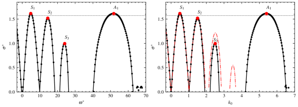
(c)

S-Modes

A-Modes

Figure 5: Stability curves of a leapfrogging wake ($R^{*}=7$, $H^{*}=5.25$, $\beta=3/4$): Dimensionless growth rate $\sigma^{*}$ as function of (a) $\omega^{*}$ and (b) $k_{0}$. For reference, fig. (b) shows the prediction for a uniform helix ($H/R=0.75$, $a_{e}/R=0.1$) in red lines. A schematic representation of the two groups of modes is shown on fig. (c), where the symmetric (resp. anti-symmetric) part is shown in red (resp. green) arrows.

(a) (b)  

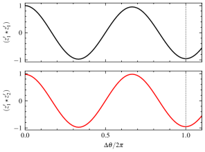
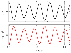
Figure 6: Function $(z_{1}^{\prime}\star z_{1}^{\prime})$ (top) and $(z_{1}^{\prime}\star z_{2}^{\prime})$ (bottom) for the case in figure 1b and modes: (a) $S_{2}$, and (b) $A_{1}$.

(a) (b)  

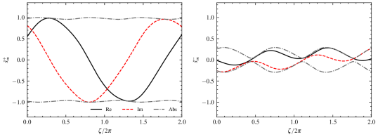
(c) (d)  

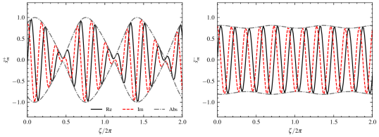
Figure 7: Complex eigenvectors for the case in figure 5. Perturbations in the local axial direction (a,c) $\check{s}_{m}^{+}$, and (b,d) $\check{s}_{m}^{-}$ shown for modes (a,b) $S_{1}$, and (c,d) $A_{1}$.

(a) (b) (c)  

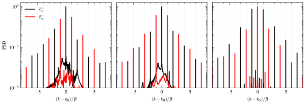
Figure 8: Fourier spectrum of modes: (a) $S_{1}$, (b) $S_{2}$, and (c) $A_{1}$, for the case in figure 5.

Mode	Frequency	Wavenumbers				Phase velocity
	$\omega^{*}$	$k_{0}$	$k_{1}$	$k_{2}$	$k_{3}$	$c_{0}$
$S_{1}$	$4.824$	$-0.500$	$(-1.250,+0.250)$	$(-2.000,+1.000)$	$(-2.750,+1.750)$	$1.002$
$S_{2}$	$14.451$	$-1.500$	$(-2.250,-0.750)$	$(-3.000,+0.000)$	$(-3.750,+0.750)$	$1.000$
$A_{1}$	$51.849$	$-5.406$	$(-6.156,-4.656)$	$(-6.906,-3.906)$	$(-7.656,-3.156)$	$0.996$

Table 2: Leading wavenumbers of the modes shown in figure 8. Here, $\Delta k=0.03125$.

Each mode displays a dominant wavenumber $k_{0}$ with additional peaks (typically in descending order of magnitude) at wavenumbers $k_{n}\approx k_{0}\pm n\beta$ for integer values of $n$ (see Fourier spectra in figures 8a-c and table 2). This pattern is also observed in the spectra of the axial and radial components, $\check{z}_{m}$ and $\check{r}_{m}$. From these observations, we infer that perturbations propagate along the structure as

$$s^{\prime}_{j}(\zeta,\psi)\approx\sum_{m}\left[\bigg{[}\hat{s}_{m0}+\sum_{n=1}\hat{s}_{mn}\cos{(n\beta\zeta/C_{\theta}+\hat{\varphi}_{mn})}\bigg{]}\cos(\omega_{m}\psi+k_{0}\zeta/C_{\theta})e^{\sigma_{m}\psi}\right]$$ (27)

where $\hat{s}_{mn}$ and $\hat{\varphi}_{mn}$ are the amplitudes and phase differences measured with respect to $k_{0}$. Consider the leading terms in (27). For symmetric modes $s_{+}^{\prime}$ roughly corresponds to a travelling wave, whereas $s_{-}^{\prime}$ approximates a wave that is modulated in amplitude by a cosine function of period $\zeta_{B}$, i.e., the periodicity of the base flow (figures 8a-b). Anti-symmetric modes display the opposite behaviour: $s_{-}^{\prime}$ approximates a travelling wave, whereas $s_{+}^{\prime}$ is modulated in amplitude by a function of period $\zeta_{B}$ (figure 8c). In both cases, the contributions from higher order terms also correspond to waves modulated in amplitude by multiples of $\zeta_{B}$ in decreasing order of magnitude.

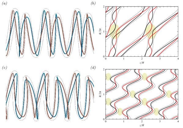
Figure 9: Base state from figure 1b perturbed by modes (a, b) $S_{1}$ and (c, d) $S_{2}$. (a, c) Three dimensional and (b, d) developed plan views illustrating the local pairing modes.

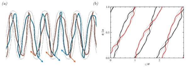
Figure 10: Base state from figure 1b perturbed by mode $A_{1}$. (a) Three dimensional and (b) developed plan view. Arrows indicate the displacements at the center plane in fig. (a).

Figure 9a presents the deformation due to the symmetric mode $S_{1}$ by plotting the perturbed geometry $\boldsymbol{X}_{j}=\boldsymbol{X}_{j}^{B}+\boldsymbol{X}_{j}^{\prime}$ for some arbitrary amplitude. A developed plan view illustrates $p=1$ localized pairing events for every $q=2$ neighbouring turns of the large-scale pattern (seen as dashed lines in figures 9a-b). An additional example corresponding to mode $S_{2}$ is shown in figures 9c-d, where $p=3$ localized pairing events are observed every $q=2$ neighbouring turns. This behaviour was expected since the predominantly aligned displacements result in a block displacement of the vortex pair. As a result, the large-scale pattern behaves like a uniform helix where perturbations with wavenumber $k_{0}=p/q$ repeat after $p$ cycles and display local pairing events at $q$ azimuthal locations (Widnall (1972)).

Anti-symmetric modes behave in a different manner. Here, the two vortices move towards (or away from) one another such that $\boldsymbol{X}_{+}$ deforms much less and only at specific positions (figure 10a). In other words, the pair predominantly displays an anti-symmetric motion with respect to the helical structure, hence the name. Displacements are localized and not necessarily aligned with the rotation of the pair. For instance, at the azimuths where displacements are perpendicular to the line connecting the two vortices the structure is twisted back and forth, whereas when displacements are parallel, the separation distance expands and contracts. The latter could potentially trigger the merging of the vortex pair. This localization can be deduced from the envelopes of the corresponding eigenvectors, illustrated as dashed lines enclosing each vortex in figure 10b. If we consider a longitudinal cut, we can see that displacements of a given vortex are paired with one of the vortices in the neighbouring turn but not with its companion (see arrows at the bottom part of figure 10a). However, the choice of the characteristic wavenumber $k_{0}$ is not obvious. For instance, doubling $H^{*}$ from $5.25$ to $10.5$ shifts mode $A_{1}$ from $k_{0}=5.406$ to $k_{0}=5.938$, while increasing $\beta$ from $3/4$ to $7/2$ shifts the wavenumber to $k_{0}=5.552$. However, perturbations between consecutive pairs remain anti-correlated, suggesting the dominant wavenumber is selected by the geometry as the one that amplifies the local pairing. We shall explore this relation in the following section.

In the appendix A, we also analyse the long-wave instability of our solutions using the linear impulse response approach developed in Durán Venegas et al. (2021). The idea is to solve the linear perturbation equation (12) using a Dirac as initial condition and analyse the spatio-temporal growth of the resulting wave packet. A sufficiently long domain is considered so that the wavepacket does not reach the boundaries during the length of the simulations. As shown in the appendix, the temporal modes can be recovered but their study is more difficult to perform with the linear impulse response as all the instability modes are simultaneously excited. However, the linear impulse response provides additional information by telling us how the instability spreads in space. In particular, we are able to show that although the most unstable anti-symmetric perturbations propagate at a similar speed than the symmetric perturbations, their spreading in space is much less important. The transition from convective to absolute instability is therefore expected to be associated with the symmetric perturbations. Moreover, as for the linear spectrum, we also demonstrate that the spatio-temporal evolution of these symmetric perturbations can be well-described by the spatio-temporal evolution of the linear impulse response on a uniform helical vortex of large core size.

4.2 Influence of $H^{*}$ and $R^{*}$ on the modes of leapfrogging wakes

(a) (b) (c)  

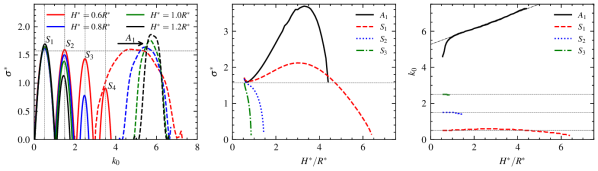
(d) (e) (f)  

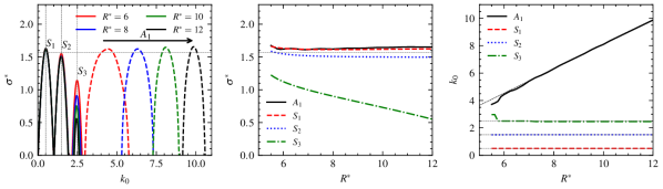
Figure 11: Growth rates and dominant wavenumbers for $\beta=3/4$. Figs. (a,b,c) shown as function of $H^{*}/R^{*}$ for $R^{*}=7$; and (d,e,f) shown as function of $R^{*}$ for $H^{*}/R^{*}=0.75$.

Since the two kinds of pairing modes described in section 4.1 seem to involve neighbouring turns of $\mathscr{H}$, growth rates are expected to display a strong dependency on the relative pitch $H^{*}/R^{*}$. In general, the maximum growth rate is larger than the maximum growth rate obtained for uniform helices with the total circulation of the vortex pair (figure 11a), which is slightly larger than $\sigma=(\pi/2)(\Gamma/H^{2})$ obtained for an array of point vortices of circulation $2\Gamma$ and separated by a distance $H$. For the range of values considered, symmetric and anti-symmetric modes have comparable growth rates (figure 11a-b). For symmetric modes, $\sigma^{*}$ initially increases for mode $S_{1}$ before vanishing, while the modes $S_{2}$, $S_{3}$, and so on, gradually vanish as the pitch increases. For anti-symmetric modes, $\sigma^{*}$ initially increases at a faster rate, but also vanishes more quickly, while the dominant wavenumber is approximated by $k_{0}=0.45H^{*}/R^{*}$ for $H^{*}/R^{*}>2$, see figure 11c.

It is also interesting to fix the relative pitch $H^{*}/R^{*}$ and change the separation distance through $R^{*}\equiv R/d$ (figure 11d). Stability curves are essentially unchanged for modes $S_{1}$ and $S_{2}$, while the growth rate of $S_{3}$ is observed to decrease as the separation distance becomes smaller (figure 11c). This is also reminiscent of uniform helical vortices, where the maximum growth rates also decrease as the effective core size becomes smaller (see, for instance figure 4). For mode $A_{1}$, the growth rate remains constant (figure 11e), while $k_{0}$ seems to evolve linearly with $k_{0}\sim 0.89R^{*}$ and overlaps the symmetric modes for $R^{*}<6$ (figure 11f).

From this dependency on $H^{*}$, and $R^{*}$, we may deduce the following: (i) $\sigma$ scales with $\Gamma/H^{2}$ for modes $A_{1}$ and $S_{1}$ whatever $H^{*}$ and $R^{*}$. This is consistent with a local pairing acting over a distance comparable to $H$; and (ii) the wavenumber most amplified by $A_{1}$ increases linearly with $H^{*}/R^{*}$ (for constant $R^{*}$) and with $R^{*}$ (for constant $H^{*}/R^{*}$). In other words, mode $A_{1}$ deviates from the classical pairing of uniform helices, and amplifies a linear wavelength $l_{0}=2\pi Rk_{0}\sim d^{-1}$ instead. This is reminiscent of a four-vortex system involving two co-rotating pairs separated by a distance $b=O(H)$ (see, for instance Crouch (1997); Fabre & Jacquin (2000)). We shall revisit this matter in section 5 with the case of $N=2$ helical pairs.

4.3 Typical displacement modes for sparsely braided wakes

(a)               (b)                

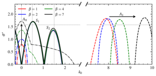
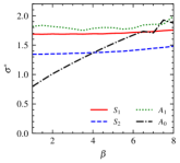
Figure 12: Stability of sparsely braided wakes for $R^{*}=10$ and $H^{*}/R^{*}=1$. (a) Growth rates and dominant wavenumbers; and (b) maximum growth rates as function of $\beta$.

(a) (b)                

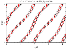
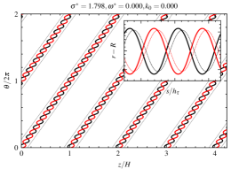
Figure 13: Base state from figure 12 and $\beta=7$ perturbed by modes (a) $S_{1}$ and (b) $A_{0}$. Figure (b) inset includes the base state (in dashed lines) for reference.

Figure 12a presents the stability curves as we move from leapfrogging to sparsely braided wakes ($1<\beta<10$). Modes $S_{1}$, $S_{2}$, and $A_{1}$, behave as in leapfrogging wakes. Some modes may act on the large-scale pattern and on the distance separating the vortex pair (see, for instance mode $S_{1}$ in figure 13a). For these modes, small oscillations in $\sigma^{*}(\beta)$ can be explained by a change in the effective distance between neighbouring vortices, which varies by a factor $d\cos(\phi)$ due to relative orientation of the vortex pairs, where $\phi=2\pi/q$ for $\beta=p/q$. For $S_{1}$ and $S_{2}$, the unstable frequencies and leading wavenumbers are unchanged, while the wavenumber most amplified by $A_{1}$ displays some dependency on $\beta$.

We observe an additional set of low frequency modes (figure 12a). Of this set of modes, the maximum growth corresponds to the zero-frequency mode $A_{0}$, which is almost a linear function of $\beta$ (figure 12b). The displacement produced by $A_{0}$ is characterized by a radial expansion of the vortex pair and a translation along the helical coordinate (see, developed plan view in figure 13b and corresponding inset). The resulting perturbed state would correspond to a similar braided wake but one with slightly larger $d$ and $R$. Other modes in the same branch display a similar displacement, but one where radial expansion and the translation along $\mathscr{H}$ are modulated in amplitude by a wavenumber $k_{0}$. For the case of two uniform helices, an equivalent displacement would yield two uniform helices of slightly larger radius. In such a case, the initial displacement is not amplified and the system remains in neutral equilibrium. However, for helical braids, the perturbed state is not necessarily a solution of (4) explaining the positive growth rate. This branch is not always present and, given the size of the parameter space ($H^{*}$, $R^{*}$, and $\beta$), it is unclear how $\sigma^{*}$ varies. For instance, for the case presented in figure 12b and $\beta=4$, $\sigma^{*}=\sigma(H^{2}/\Gamma)$ is close to $1.5$. For the same $(R^{*},\beta)$ and $H^{*}/R^{*}=2$, $\sigma^{*}$ is nearly four times larger, suggesting these modes no longer scale with $\Gamma/H^{2}$. This behaviour extends to the case of densely braided wakes.

4.4 Typical displacement modes for densely braided wakes

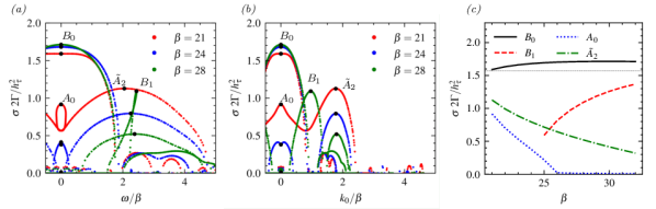
Figure 14: Stability of densely braided wakes for $R^{*}=10$ and $H^{*}/R^{*}=1$: growth rate as function of (a) $\omega$ and (b) $k_{0}$ for different $\beta$; and (c) growth rate of modes identified in figs. (a,b) as function of $\beta$.

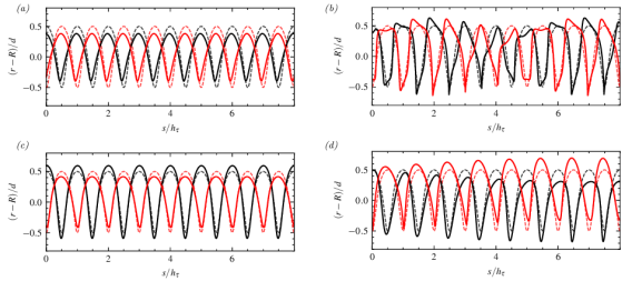
Figure 15: Stability of densely braided wakes. Schematic representation of the displacement modes identified in figure 14: (a) $A_{0}$, (b) $\tilde{A}_{2}$, (c) $B_{0}$, and (d) $B_{1}$. For reference, each figure also includes the base state (in dashed lines).

Densely braided wakes correspond to the case $\beta>10$, when the pitch $h_{\tau}$ becomes of the same order as the separation distance $d$ and the pairing modes of the vortex pair become dominant. The stability curves in figure 14a-b, display nearly all of the modes introduced so far. Modes $S_{1}$, $S_{2}$, and $A_{1}$ remain unchanged but are dwarfed by the other modes. For $\beta=21$, the branch containing mode $A_{0}$ is still present, and now contains a new local maxima around $k_{0}/\beta=2$, denoted $\tilde{A}_{2}$ in figure 14b. For $\beta=24$, the branch containing both modes splits in two. Modes $A_{0}$ and $\tilde{A}_{2}$ display a similar scaling and seem to vanish for large $\beta$ (figure 14c). The spatial structure of $A_{0}$ is unchanged (see, figure 13b inset and 15a), while mode $\tilde{A}_{2}$ displays a radial expansion modulated in amplitude with some spatial frequency (figure 15b).

Finally, we have the pairing modes of the vortex pair. For these modes, the scaling of the growth rate is different since the pairing acts over a distance comparable to $h_{\tau}/2$ instead of $H$. The maximum growth rate is comparable to the predictions for two interlaced helices and $\sigma=(\pi/2)(2\Gamma/h_{\tau}^{2})$ obtained for an array of point vortices of circulation $\Gamma$ and separated by $h_{\tau}/2$ (figure 14c). Here, mode $B_{0}$ corresponds to a special case with $\omega=0$ and $k_{0}=0$. As shown in figure 15c, displacements are characterized by a radial expansion of the vortex pair and a translation along the helical coordinate for one vortex, and a radial contraction and a translation in the opposite direction for the other one. This results in a form of uniform pairing along the helical coordinate, analogous to the global pairing mode of two uniform helices. For $\beta>25$, a second maximum, denoted $B_{1}$, is observed near $k_{0}/\beta=1$. As shown in figure 15d, displacements approach the vortices in neighbouring turns at specific intervals, analogous to the local pairing mode of two uniform helices.

5 Stability of two vortex pair with central hub vortex

A similar stability analysis can be performed for the case of two interlaced vortex pairs with a central hub vortex, illustrated in figure 1c. For this analysis, we considered the hub as a straight vortex. Contribution from the hub are taken into account for the stability analysis but the hub itself was not allowed to deform. We present only the modes corresponding to leapfrogging wakes and focus on the differences with respect to the case of one helical pair. Unstable modes associated with braided wakes are not discussed, but we expect them to display roughly the same behaviour described in section 4.

5.1 Typical displacement modes for leapfrogging wakes

(a) (b)                

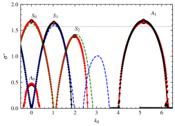
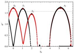
Figure 16: Stability curves for the case of two helical pairs (a) without and (b) with a central hub vortex and ($R^{*}=7$, $H^{*}/R^{*}=1.5$, $\beta=3/4$). Colour indicates the phase difference between the two helical pairs: $\varphi=0$ (in black), $\varphi=\pi$ (in red). For reference, fig (a) includes the values for two uniform helices ($H/R=1.5$, $a_{e}/R=0.1$) in dashed lines.

(a) (b)  

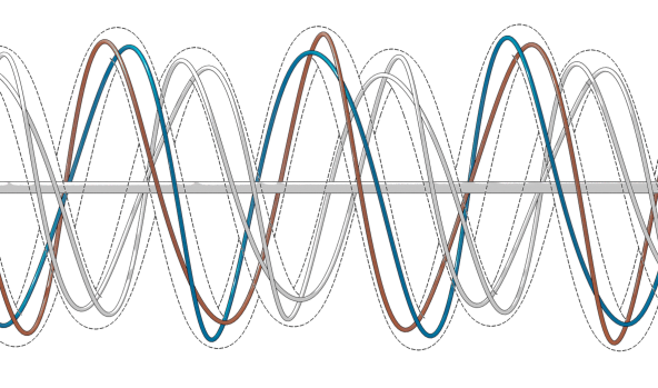
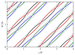
Figure 17: (a) Three dimensional view of the base state from figure 1c perturbed by mode $S_{0}$, and (b) developed plan view illustrating the global pairing.

Mode	Frequency	Wavenumbers				Phase velocity
	$\omega^{*}$	$k_{0}$	$k_{1}$	$k_{2}$	$k_{3}$	$c_{0}$
$S_{0}$	$0.015$	$0.000$	$(-0.781,+0.719)$	$(-1.531,+1.469)$	$(-2.281,+2.219)$	$0.952$
$S_{1}$	$9.863$	$-1.031$	$(-1.781,+0.281)$	$(-2.531,+0.469)$	$(-3.281,+1.219)$	$0.987$
$S_{2}$	$19.086$	$-2.000$	$(-2.750,-1.250)$	$(-3.500,-0.500)$	$(-4.250,+0.250)$	$0.984$
$A_{1}$	$51.846$	$-5.468$	$(-6.219,-4.719)$	$(-6.969,-3.969)$	$(-7.719,-1.719)$	$0.978$

Table 3: Leading wavenumbers of the modes shown in figure 16. Here, $\Delta k=0.03125$.

We consider similar geometric parameters as in §4.1, but increase the pitch as to preserve the mean axial distance between neighbouring turns. The results are summarized in figures 16, 17 and 18. The frequency spectra presented in figure 16a is characterized by a first set of modes distributed over three overlapping lobes at low frequencies, and a second set distributed over two additional lobes at higher frequencies and a small lobe containing $A_{0}$. As in the previous case, the former are symmetric modes, the latter are anti-symmetric. The structure of the eigenvectors is the same as before with dominant wavenumbers at $k_{0}$ and additional harmonic terms at $k_{n}=k_{0}\pm n\beta$, see table 3. In general, the maximum growth rate is larger than the maximum growth rate obtained for two uniform helices with the total circulation of each vortex pair, which is slightly larger than $\sigma=(\pi/2)(2\Gamma/H^{2})$ obtained for an array of point vortices of circulation $2\Gamma$ and separated by a distance $H/2$.

As expected, symmetric modes are reminiscent of the unstable modes obtained for two equivalent helical vortices. Displacements between neighbouring turns are out-of-phase for modes in the branch containing $S_{0}$ and $S_{2}$ (in black), and phase-aligned for modes in the branches containing $S_{1}$ and $S_{3}$ (in red). These displacements result in a local pairing at $2k$ azimuthal positions per turn of the large-scale helix. Mode $S_{0}$ corresponds to a special case. Displacements between neighbouring turns are out-of-phase, where one vortex pair expands in the radial direction, while the other one contracts, resulting in a uniform pairing of the large-scale pattern along the azimuthal direction (figures 17a-b). This is analogous to the global pairing mode $k=0$ of the interlaced helices (see, for instance Okulov & Sørensen (2009); Quaranta et al. (2019)).

Additionally, we note that anti-symmetric modes are observed over a similar range of values as in the case of one vortex pair. One notable difference is that two modes are now obtained for the same $k_{0}$ (each using a different colour in figure 16a), where each pair has a similar structure but shifted in phase (not shown).

The introduction a central hub vortex ensures the total circulation to be zero and the angular velocity to vanish as $r\to\infty$. This has a small effect on the frame velocity and the base state with and without central hub are qualitatively similar. The presence of a central hub modifies the stability properties to a small degree (figures 16b). For instance, the case with a central hub vortex has generally larger growth rates than the case without by 2-3%. Additionally, the branches containing $A_{0}$ are suppressed by the hub vortex, while the out-of-phase perturbations are no longer neutrally stable near $k_{0}=1$. In the following, we consider only the case with a central hub.

5.2 Geometric dependency of the most unstable modes

(a) (b) (c)  

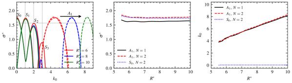
(d) (e) (f)  

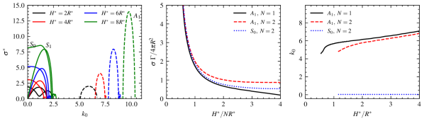
Figure 18: (a,d) Stability curves, (b,e) growth rates and (c,f) dominant wavenumbers as function of $R^{*}$ for $(H^{*}/R^{*}=1.5,\beta=3/4)$ (a,b,c), and as function of $H^{*}/R^{*}$ for $(R^{*}=7,\beta=3/4)$ (d,e,f).

As expected, symmetric and anti-symmetric modes display a different behaviour as we vary the geometric parameters. Varying the separation distance has a small influence on the symmetric modes. As in case of one vortex pair, the change in growth rates is reminiscent to that of varying the effective core size in uniform helices: small for $S_{0}$ and $S_{1}$, but more important for higher wavenumbers (figure 18a). For anti-symmetric modes, the change in growth rates is also small (figure 18b), while the dominant wavenumber $k_{0}$ increases linearly with $R^{*}$ (figure 18c). For $H^{*}/R^{*}=1.5$, $k_{0}$ was found to be roughly the same as in the case of one vortex pair with equal effective pitch, suggesting the modes are selected by the same pairing mechanism described in §4.

Varying the relative pitch shows the transition between two different regimes. For small $H^{*}/R^{*}$, stability curves have a similar structure as before: symmetric modes distributed over two or more branches with small $k_{0}$ and anti-symmetric modes distributed over two overlapping branches with larger $k_{0}$. Growth rates are larger than predicted rates for the equivalent uniform helices, but still close to the point vortex prediction $\sigma\sim\Gamma N^{2}/H^{2}$. For large $H^{*}/R^{*}$, the stability curves are characterized by two branches at small $k_{0}$ containing modes $S_{0}$ and $S_{1}$, and single branch containing $A_{1}$ at larger $k_{0}$. Modes $S_{1}$ and $A_{1}$ are shifted towards larger wavenumbers. Instead of vanishing, the dimensionless growth rate $\sigma^{*}$ proceeds to increase, pointing to a different scaling law with $\sigma\sim\Gamma/R^{2}$ for large $H^{*}/R^{*}$ (figures 16d-e). A similar transition is observed for the most unstable wavenumber $k_{0}$: $k_{0}\sim H^{*}/NR^{*}$ for small $H^{*}/R^{*}$, and $k_{0}\sim H^{*}/R^{*}$ for large $H^{*}/R^{*}$ (figure 18f).

This change of regime can be understood as follows. For the case a single pair ($N=1$), the limit of large $H^{*}/R^{*}$ leads to a pair of parallel co-rotating vortices which are known to be stable with respect to long wavelength perturbations (Jimenez, 1975). For the case of $N=2$ vortex pairs with a central hub, the same limit provides a system composed of two co-rotating pairs of vortices of circulation $\Gamma$ and one counter-rotating vortex of circulation $-4\Gamma$ at the centre. For this configuration, the instability is necessarily controlled by the distance between the vorticity centroids ($b=2R$ in our current notation), and the separation distance $d$. This configuration is similar to four-vortex systems (Crouch, 1997; Fabre et al., 2002), which are known to be unstable, with a maximum growth rate scaling with $\Gamma/b^{2}$, and a most unstable wavenumber varying with $b$ and $d$.

6 Discussion

(a)  

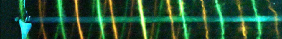
(b)  

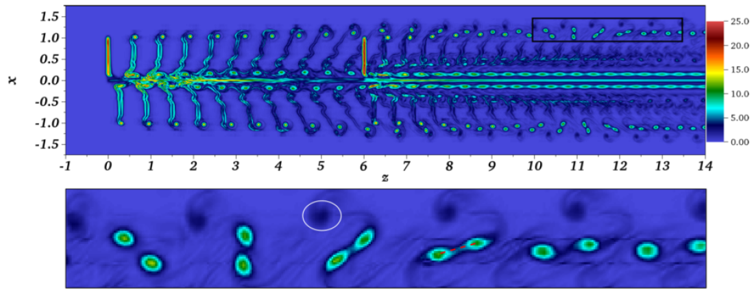
Figure 19: (a) Experimental dye visualisation for a two-bladed rotor with 1.5% radial rotor offset taken Quaranta et al. (2019). (b) Vorticity contours for two in-line wind turbines from Kleine et al. (2019). A close-up of the vortex interaction is shown at the bottom.

In this article, we have studied the long-wave stability properties of closely-spaced helical vortex pairs using a cut-off filament approach. The considered base flow configuration corresponds to the far-wake produced by a rotor emitting two distinct vortices near the tips of each blade and which was studied previously in (Castillo-Castellanos et al., 2021). Both the temporal linear spectrum and the linear impulse response have been analysed, but the linear spectrum has been found to be much more convenient to identify the different instability modes.

We have classified these modes in different groups. Symmetric modes are characterized by a block displacement of the vortex pair, analogous to the local pairing modes in helical geometries. Anti-symmetric modes are characterized by a mirrored displacement with respect to the vorticity centre of the pair, with the most unstable mode corresponding to a local pairing between one member of a pair with the other member of a pair in the neighbouring turn. These modes are particularly important since they could trigger the merging of vortex pairs. Additional modes are observed as we increase the twist parameter $\beta$: one corresponds to a radial expansion of the pair and a displacement along the centerline helix, while the other corresponds to the global and local pairing modes of the vortex pair, analogous to the case of two interlaced helices obtained by straightening the centerline helix. We have also considered the dependency of the stability properties with respect to the relative pitch, the separation distance, and the twist parameter. We have identified the regions in the parameter space where each mode is dominant. Our observations also suggest that the pairing mechanism associated with the anti-symmetric modes amplifies a specific axial wavelength (in the developed plane) instead of an azimuthal wavelength, reminiscent of the anti-symmetric modes observed in four-vortex systems. A similar pairing mechanism has also been observed for the case of two pairs of helical vortices with one central hub. However, in this case, the instability does not disappear in the limit of large pitch and exhibits a maximum growth rate scaling with $R/d$. Additional, the central hub was found to have only a small influence on the stability properties.

Experimental devices with 8cm and 24cm radius by Schröder et al. (2020, 2021) successfully generated a pair of tip vortices. Their main objective was to obtain a larger and less intense tip vortex. In their case, tip vortices were unstable with respect to a centrifugal instability due to patches of opposite signed vorticity remaining from the roll-up process. This instability triggered the vortex merging long before the long-wave instabilities could be observed. We speculate that it could be possible to delay such instability by carefully tuning the blade geometry, or by considering a larger rotor. Since core sizes typically scale with the chord length, very large rotors could generate well separated tip vortices with stable cores. Because of the vortex diffusion, merging is expected even in the absence of external perturbations and would depend on the ratio between the core radii and the separation distance. External perturbations would only accelerate this process. Anti-symmetric modes are expected to trigger the merging faster than symmetric modes. However, this would require a form of active control. Since, anti-symmetric modes are excited by larger temporal and spatial frequencies, it is possible they could be more easily excited by atmospheric turbulence than symmetric modes.

Helical pairs are not necessarily limited to the case of a tip-splitting rotor. One alternative to generate a helical pair would be to consider asymmetric rotors. As shown in Quaranta et al. (2019), a radial asymmetry excites the global pairing mode to obtain a remarkably coherent structure like the one displayed in figure 19a. From a topology perspective, this structure is consistent with a leapfrogging wake with $d\sim H/2$ and $\beta\ll 1$, where the value of $\beta$ is controlled by the radial offset. This is a promising approach since existing wind turbines could be easily modified. A similar result can be obtain using an axial offset, as in the case of two in-line wind turbines considered by Kleine et al. (2019). If the axial offset is not too large and is a multiple of the pitch, we may expect the interaction between tip vortices result in $N$ pairs of helical vortices downstream, like the ones displayed in figure 19b. As observed in figure 5 of Kleine et al. (2019), unstable dynamical modes are either in phase-alignment or in phase-opposition, similar to the symmetric and anti-symmetric modes presented here.

Our analysis assumes the wavelength of the displacement perturbations to be large with respect to the core size. For helical vortices, Quaranta et al. (2015) estimated the limit of validity in the form of wavenumber $k\leq k_{l}$. For the values used in figure 10, this upper limit corresponds to $k_{l}\approx 0.40(a_{e}/R)^{-1}$ and $k_{l}\approx 1.60(a_{e}/d)^{-1}$. Since we consider slender vortex filaments ($a_{e}/R\sim 0.01$ and $a_{e}/d\sim 0.1$), the limit of validity of the long-wave approximation should not be a concern. Unlike Quaranta et al. (2015), which uses analytical expressions, our approach considers the filaments as a sequence of straight segments to compute the Jacobian matrix using semi-analytical expressions. This approach has been validated using known results for the long-wave instability of uniform helices. However, it is more general as it does not require prior knowledge of the spatial structure of the instability modes. It also provides the complete spectrum and applies to any stationary vortex solution, like the ones in figure 19.

By using a filament approach, we have neglected what is occurring in the vortex cores. Yet, vortex cores are expected to be distorted by curvature and straining effects (Blanco-Rodríguez et al., 2015). Moreover, these deformations are also responsible for the short-wave instabilities developing in vortex cores. Depending on the geometric parameters, these short-wave instabilities can become dominant. For instance, the elliptical instability is expected to grow with $\Gamma/d^{2}$ instead of $\Gamma/H^{2}$ although with different pre-factors (Roy et al., 2008; Blanco-Rodríguez & Le Dizès, 2016), while the curvature instability (Blanco-Rodríguez & Le Dizès, 2017) is also expected to be present and important if the vortex core exhibits an axial jet. None of these have been considered here. However, Brynjell-Rahkola & Henningson (2020) have shown that it is indeed possible to analyse the stability of uniform helical vortices with respect to both short and large wavelengths using a DNS from an initial condition obtained by the filament solutions together with a prescribed vortex model in the cores. It would be interesting to implement such an approach to our configurations in order to analyse the competition between both instabilities.

[Acknowledgements] The authors are grateful to Eduardo Durán Venegas and Thomas Leweke for their valuable contributions.

[Funding] This work is part of the French-German project TWIN-HELIX, supported by the Agence Nationale de la Recherche (grant no. ANR-17-CE06-0018) and the Deutsche Forschungsgemeinschaft (grant no. 391677260).

[Declaration of interests]The authors report no conflict of interest.

[Author ORCID] A. Castillo-Castellanos, https://orcid.org/0000-0003-2175-324X; S. Le Dizès, https://orcid.org/0000-0001-6540-0433

Appendix A Space-time impulse response

A.1 Methodology

The space-time impulse response of $\boldsymbol{X}_{j}^{B}$ is studied as in Durán Venegas et al. (2021). We introduce a Dirac impulse as to excite all the wavenumber components with equal amplitude and follow the evolution of the resulting wavepacket. We consider two types of initial perturbation as to preferentially excite the symmetric and anti-symmetric modes

$$\boldsymbol{q}_{0}^{\prime}(\zeta)=\begin{cases}(0,0,A_{0}\delta(\zeta-\zeta_{p}),0,0,~{}~{}A_{0}\delta(\zeta-\zeta_{0}))&\mbox{Case A (in-phase)}\\ (0,0,A_{0}\delta(\zeta-\zeta_{p}),0,0,-A_{0}\delta(\zeta-\zeta_{0}))&\mbox{Case B (out-of-phase)}\end{cases}$$ (28)

where $A_{0}$ and $\zeta_{0}$ indicate the amplitude and wake coordinate of the initial perturbation and $\delta$ is the Dirac delta function. Then, we use (12) recursively to obtain $\boldsymbol{q}^{\prime}(\zeta,\psi=m\Delta\psi)$ for $(m=1,2,\cdots)$ until the exponential regime is established. In general, the exponential regime is established quickly and our calculation domain is considered to be long enough to avoid boundary effects.

Temporal growth rates are estimated from the impulse response as follows. At each time $\psi$, we apply the spatial Fourier transform along $\zeta$ to the axial displacement. Then, for each azimuthal wavenumber $k$ we can monitor the amplitude of each Fourier mode and estimate its growth rate by

$$\sigma_{j}(k)\approx\frac{\partial(\log\lVert\hat{z}^{\prime}_{j}(k)\rVert)}{\partial\psi}.$$ (29)

It is also interesting to consider the growth rate

$$\sigma_{V}(V_{\psi})\approx\frac{\log(|z^{\prime}_{j}(\psi,\zeta_{0}+V_{\psi}\psi)|)}{\psi}$$ (30)

in the frame moving along the vortex structure with an angular velocity $V_{\psi}$. In particular, we are interested in the velocity $V_{\psi}^{\max}$ at which the growth rate is maximum and the upper and lower limits at which the perturbation grows, $V_{\psi}^{+}$ and $V_{\psi}^{-}$. This provides a quantitative criterium to identify convectively unstable and absolutely unstable flows (Huerre & Monkewitz, 1990).

A.2 Stability curves from the impulse response

(a) (b)  

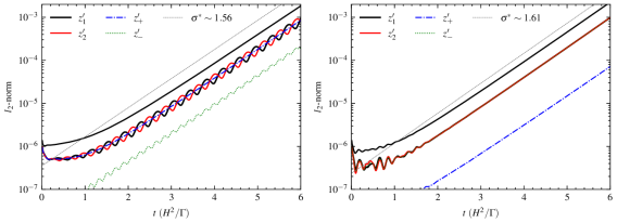
Figure 20: Linear impulse response for ($R^{*}=10$, $H^{*}/R^{*}=0.75$, $\beta=1$). (a,b) $l_{2}$-norm of the perturbations for cases A and B, respectively.

Consider the propagation of the initial perturbation corresponding to case A. The norm of the total displacement $\boldsymbol{q}^{\prime}$ grows exponentially with constant rate $\sigma^{*}$ while the axial displacements $z_{1}^{\prime}$ and $z_{2}^{\prime}$ display variable growth rates with a period comparable to the characteristic time of the vortex pair (figure 20a). The symmetric component $z_{+}^{\prime}$ is dominant and displays a constant growth rate equal to $\sigma^{*}$. A similar behaviour is observed for radial and angular displacements (not shown). The spatio-temporal evolution corresponding to case B provides similar growth rates, but $z_{-}^{\prime}$ is now dominant and the oscillations in $z_{1}^{\prime}$ and $z_{2}^{\prime}$ are less pronounced (figure 20b). Cases A and B have slightly different growth rates, illustrating a clear dependency on the initial conditions (figure 20a and 20b). The observed growth rates correspond to the predicted rates for the most unstable symmetric and anti-symmetric modes, $S_{1}$ and $A_{1}$, respectively. As expected, if we observe long enough both cases eventually arrive to whichever one with the largest growth rate.

(a) (b) (c)  

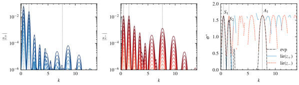
Figure 21: Fourier amplitudes of (a) $z_{+}^{\prime}$ and (b) $z_{-}^{\prime}$ for case A, where each line corresponds to a different instant at regular intervals, and (c) corresponding growth rates obtained using (29) compared to results from the eigenvalue problem.

(a) (b) (c)  

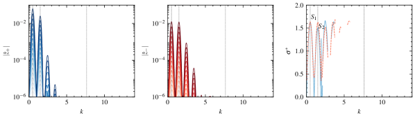
(d) (e) (f)  

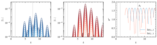
Figure 22: Fourier amplitudes of (a,d) $z_{+}^{\prime}$ and (b,e) $z_{-}^{\prime}$, where each line corresponds to a different instant, and (c,d) growth rates obtained using (29). Figs. (a-c) correspond to case A with a high-pass filter, and figs. (d-f) to case B with a low-pass filter, see text.

Figure 21a (resp. 21b) displays the Fourier spectra of $z_{+}^{\prime}$ (resp. $z_{-}^{\prime}$) taken at regular intervals, where the most unstable wavenumbers are clearly identified. For each wavenumber $k$, the corresponding growth rate obtained using (29) is shown in figure 21c. Results are in good agreement with the eigenvalue problem (dash-dotted lines). For instance, in $z_{+}^{\prime}$ the most unstable wavenumbers correspond to the dominant wavenumbers of $S_{1}$ and $S_{2}$. Additional peaks in $z_{+}^{\prime}$ (in blue) correspond to even harmonics, while peaks in $z_{-}^{\prime}$ (in orange) correspond to odd harmonics of $S_{1}$. Similar results are observed for mode $A_{1}$ and to a smaller degree for mode $S_{2}$.

Issues in recovering the harmonics of mode $S_{2}$ can be explained by the overlapping with other modes. We may take advantage of the separation in temporal frequency to reduce this effect. For instance, applying a high-pass filter to the wave-packets from case A before evaluating the Fourier coefficients, i.e., filtering the anti-symmetric modes, we recover the growth rates of symmetric modes over a wider range of wavenumbers (figures 22a-c). Conversely, applying a low-pass filter to the wave-packets from case B, i.e., filtering the symmetric modes, we recover the growth rates of anti-symmetric modes over a similar range (figures 22d-f). Superimposing the growth rates obtained from cases A and B, we obtain a more complete picture of the stability curves, in good agreement with results from section 4.

(a) (b) (c)  

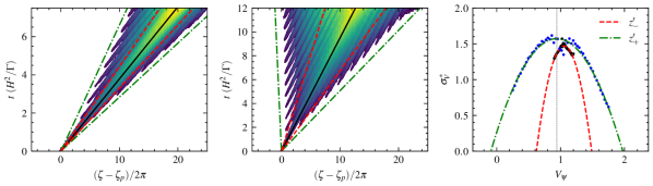
Figure 23: Impulse response for ($R^{*}=10$, $\beta=1$) and case B: contours of $\log(|z^{\prime}_{1}|)$ for (a) $H^{*}/R^{*}=0.75$ and (b) $H^{*}/R^{*}=0.5$ ; and (c) $\sigma_{V}^{*}$ as function of $V_{\psi}$ for the case in figure (b). Here, $z^{\prime}_{+}$ and $z^{\prime}_{-}$, spread at different rates shown in green and red lines.

A.3 Space-time evolution of perturbations

Figures 23a and 23b display the space-time evolution of the initial perturbation corresponding to case B. In both cases, perturbations initially propagate in a narrow wavepacket of high (temporal) frequency content associated with anti-symmetric modes, before a second wavepacket with lower frequencies typical of symmetric modes is observed. The case in figure 23a corresponds to a convective instability, while the one in figure 23b illustrates the transition to an absolute instability. Despite the overlapping of frequencies and wavenumbers, it is still possible to estimate the front velocities using (30) by considering separately the symmetric and anti-symmetric parts, $z^{\prime}_{+}$ and $z^{\prime}_{-}$. The maximum growth rate corresponds to a velocity $V_{\psi}=V_{\psi}^{\max}$ close to the phase velocity $c_{0}$ of the most unstable modes (see, peak value in figure 23c and black lines in figures 23a-b). In general, the anti-symmetric wavepacket (in dashed red lines) spreads more slowly than symmetric part (in dash-dotted green lines), suggesting that the transition from convective to absolute instability can be monitored by following the spread of the symmetric part. As expected, the growth rate $\sigma_{V}^{*}$ of the symmetric part behaves similarly to the equivalent helical vortex and is well approximated by the predicted growth rate for a periodic array of point vortices as proposed by Durán Venegas et al. (2021)

$$\sigma_{V}^{*}=(\pi/2)(1-(V_{rel}^{*})^{2})$$ (31)

where $V_{rel}^{*}=(V_{\psi}-V_{\psi}^{\max})(2\pi/\Omega_{R})/t_{adv}$ is the frame velocity relative to the advection frame.

References

- Bayly (1988) Bayly, B. J. 1988 Three-dimensional centrifugal-type instabilities in inviscid two-dimensional flows. Phys. Fluids 31 (1), 56–64.
- Bhagwat & Leishman (2000) Bhagwat, M. J. & Leishman, J. G. 2000 Stability analysis of helicopter rotor wakes in axial flight. J. Amer. Helic. Soc. 45 (3), 165.
- Blanco-Rodríguez & Le Dizès (2016) Blanco-Rodríguez, F. J. & Le Dizès, S. 2016 Elliptic instability of a curved batchelor vortex. J. Fluid Mech. 804, 224–247.
- Blanco-Rodríguez & Le Dizès (2017) Blanco-Rodríguez, F. J. & Le Dizès, S. 2017 Curvature instability of a curved batchelor vortex. J. Fluid Mech. 814, 397–415.
- Blanco-Rodríguez et al. (2015) Blanco-Rodríguez, F. J., Le Dizès, S., Selçuk, C., Delbende, I. & Rossi, M. 2015 Internal structure of vortex rings and helical vortices. J. Fluid Mech. 785, 219–247.
- Brocklehurst & Pike (1994) Brocklehurst, A. & Pike, A.C. 1994 Reduction of BVI noise using a vane tip. In AHS Aeromechanics Specialists Conference. American Helicopter Society.
- Brown et al. (2022) Brown, K., Houck, D., Maniaci, D., Westergaard, C. & Kelley, C. 2022 Accelerated wind-turbine wake recovery through actuation of the tip-vortex instability. AIAA Journal pp. 1–13.
- Brynjell-Rahkola & Henningson (2020) Brynjell-Rahkola, M. & Henningson, D. S. 2020 Numerical realization of helical vortices: application to vortex instability. Theor. Comp. Fluid Dyn 34 (1), 1–20.
- Cañadillas et al. (2020) Cañadillas, B., Foreman, R., Barth, V., Siedersleben, S., Lampert, A., Platis, A., Djath, B., Schulz-Stellenfleth, J., Bange, J., Emeis, S. & others 2020 Offshore wind farm wake recovery: Airborne measurements and its representation in engineering models. Wind Energy 23 (5), 1249–1265.
- Castillo-Castellanos et al. (2021) Castillo-Castellanos, A., Le Dizès, S. & Durán Venegas, E. 2021 Closely spaced corotating helical vortices: General solutions. Phys. Rev. Fluids 6, 114701.
- Crouch (1997) Crouch, J.D. 1997 Instability and transient growth for two trailing-vortex pairs. J. Fluid Mech. 350, 311–330.
- Crow (1970) Crow, S. C. 1970 Stability theory for a pair of trailing vortices. AIAA journal 8 (12), 2172–2179.
- Durán Venegas & Le Dizès (2019) Durán Venegas, E. & Le Dizès, S. 2019 Generalized helical vortex pairs. J. Fluid Mech. 865, 523–545.
- Durán Venegas et al. (2021) Durán Venegas, E., Rieu, P. & Le Dizès, S. 2021 Structure and stability of Joukowski’s rotor wake model. J. Fluid Mech. 911, A6.
- Fabre & Jacquin (2000) Fabre, D. & Jacquin, L. 2000 Stability of a four-vortex aircraft wake model. Phys. Fluids 12 (10), 2438–2443.
- Fabre et al. (2002) Fabre, D., Jacquin, L. & Loof, A. 2002 Optimal perturbations in a four-vortex aircraft wake in counter-rotating configuration. J. Fluid Mech. 451, 319.
- Frederik et al. (2020) Frederik, J. A., Doekemeijer, B. M., Mulders, S. P. & van Wingerden, J.-W. 2020 The helix approach: Using dynamic individual pitch control to enhance wake mixing in wind farms. Wind Energy 23 (8), 1739–1751.
- Fukumoto & Miyazaki (1991) Fukumoto, Y. & Miyazaki, T. 1991 Three–dimensional distorsions of a vortex filament zith axial velocity. J. Fluid Mech. 222, 369–416.
- Gupta & Loewy (1974) Gupta, B.P. & Loewy, R.G. 1974 Theoretical analysis of the aerodynamic stability of multiple, interdigitated helical vortices. AIAA J. 12 (10), 1381–1387.
- Hardin (1982) Hardin, J. C. 1982 The velocity field induced by a helical vortex filament. Phys. Fluids 25 (11), 1949–1952.
- Huang et al. (2019) Huang, X., Moghadam, S. M. A., Meysonnat, P.S., Meinke, M. & Schröder, W. 2019 Numerical analysis of the effect of flaps on the tip vortex of a wind turbine blade. Int. J. Heat Fluid Flow 77, 336–351.
- Huerre & Monkewitz (1990) Huerre, P. & Monkewitz, P. A. 1990 Local and global instabilities in spatially developing flows. Annu. Rev. Fluid Mech. 22 (1), 473–537.
- Ivanell et al. (2010) Ivanell, S., Mikkelsen, R., Sørensen, J. N. & Henningson, D. 2010 Stability analysis of the tip vortices of a wind turbine. Wind Energy 13 (8), 705–715.
- Jimenez (1975) Jimenez, J. 1975 Stability of a pair of co-rotating vortices. Phys. Fluids 18 (11), 1580–1581.
- Josserand & Rossi (2007) Josserand, Ch. & Rossi, M. 2007 The merging of two co-rotating vortices: a numerical study. European Journal of Mechanics-B/Fluids 26 (6), 779–794.
- Kawada (1936) Kawada, S. 1936 Induced velocity by helical vortices. J. Aeronaut. Sci. 3 (3), 86–87.
- Kerswell (2002) Kerswell, R. R. 2002 Elliptical instability. Annu. Rev. Fluid Mech. 34 (1), 83–113.
- Kleine et al. (2019) Kleine, V.G., Kleusberg, E., Hanifi, A. & Henningson, D.S. 2019 Tip-vortex instabilities of two in-line wind turbines. In Journal of Physics: Conference Series, , vol. 1256, p. 012015. IOP Publishing.
- Lamb (1945) Lamb, H. 1945 Hydrodynamics. Dover publications.
- Leishman et al. (2002) Leishman, J. G., Bhagwat, M. J. & Bagai, A. 2002 Free-vortex filament methods for the analysis of helicopter rotor wakes. J Aicr 39 (5), 759–775.
- Levy & Forsdyke (1928) Levy, H. & Forsdyke, A. G. 1928 The steady motion and stability of a helical vortex. Proc. R. Soc. Lond. A 120, 670–690.
- Leweke et al. (2016) Leweke, T., Le Dizes, S. & Williamson, C. H.K. 2016 Dynamics and instabilities of vortex pairs. Annu. Rev. Fluid Mech. 48 (1), 507–541.
- Leweke et al. (2014) Leweke, T., Quaranta, H. U., Bolnot, H., Blanco-Rodriíguez, F. J. & Le Dizès, S. 2014 Long- and short-wave instabilities in helical vortices. J. Phys.: Conf. Ser. 524, 012154.
- Meunier et al. (2002) Meunier, P., Ehrenstein, U., Leweke, T. & Rossi, M. 2002 A merging criterion for two-dimensional co-rotating vortices. Phys. Fluids 14 (8), 2757–2766.
- Meunier & Leweke (2005) Meunier, P. & Leweke, T. 2005 Elliptic instability of a co-rotating vortex pair. J. Fluid Mech. 533, 125–159.
- Okulov (2004) Okulov, V. L. 2004 On the stability of multiple helical vortices. J. Fluid Mech. 521, 319–342.
- Okulov & Sørensen (2007) Okulov, V. L. & Sørensen, J. N. 2007 Stability of helical tip vortices in a rotor far wake. J. Fluid Mech. 576, 1–25.
- Okulov & Sørensen (2009) Okulov, V. L. & Sørensen, J. N. 2009 Applications of 2d helical vortex dynamics. Theor. Comp. Fluid Dyn 24 (1-4), 395–401.
- Quaranta et al. (2015) Quaranta, H. U., Bolnot, H. & Leweke, T. 2015 Long-wave instability of a helical vortex. J. Fluid Mech. 780, 687–716.
- Quaranta et al. (2019) Quaranta, H. U., Brynjell-Rahkola, M., Leweke, T. & Henningson, D. S. 2019 Local and global pairing instabilities of two interlaced helical vortices. J. Fluid Mech. 863, 927–955.
- Robinson & Saffman (1982) Robinson, A. C. & Saffman, P. G. 1982 Three-dimensional stability of vortex arrays. J. Fluid Mech. 125, 411.
- Roy et al. (2008) Roy, C., Schaeffer, N., Le Dizès, S. & Thompson, M. 2008 Stability of a pair of co-rotating vortices with axial flow. Phys. Fluids 20 (9), 094101.
- Schröder et al. (2020) Schröder, D., Leweke, T., Hörnschemeyer, R. & Stumpf, E. 2020 Experimental investigation of a helical vortex pair. In Deutscher Luft-und Raumfahrtkongress 2020.
- Schröder et al. (2021) Schröder, D., Leweke, T., Hörnschemeyer, R. & Stumpf, E. 2021 Instability and merging of a helical vortex pair in the wake of a rotor. J. Phys.: Conf. Ser. 1934 (1), 012007.
- Selçuk et al. (2017) Selçuk, C., Delbende, I. & Rossi, M. 2017 Helical vortices: Quasiequilibrium states and their time evolution. Phys. Rev. Fluids 2 (8), 084701.
- Walther et al. (2007) Walther, J. H., Guénot, M., Machefaux, E., Rasmussen, J. T., Chatelain, P., Okulov, V. L., Sørensen, J. N., Bergdorf, M. & Koumoutsakos, P. 2007 A numerical study of the stabilitiy of helical vortices using vortex methods. J. Phys.: Conf. Ser. 75, 012034.
- Widnall (1972) Widnall, S. E. 1972 The stability of a helical vortex filament. J. Fluid Mech. 54 (4), 641–663.