Analysis of Generalized Bregman Surrogate Algorithms for Nonsmooth Nonconvex Statistical Learning

Abstract

Modern statistical applications often involve minimizing an objective function that may be nonsmooth and/or nonconvex. This paper focuses on a broad Bregman-surrogate algorithm framework including the local linear approximation, mirror descent, iterative thresholding, DC programming and many others as particular instances. The recharacterization via generalized Bregman functions enables us to construct suitable error measures and establish global convergence rates for nonconvex and nonsmooth objectives in possibly high dimensions. For sparse learning problems with a composite objective, under some regularity conditions, the obtained estimators as the surrogate’s fixed points, though not necessarily local minimizers, enjoy provable statistical guarantees, and the sequence of iterates can be shown to approach the statistical truth within the desired accuracy geometrically fast. The paper also studies how to design adaptive momentum based accelerations without assuming convexity or smoothness by carefully controlling stepsize and relaxation parameters.

, and

1 Introduction

Many statistical learning problems can be formulated as minimizing a certain objective function. In shrinkage estimation, the objective can often be represented as the sum of a loss function and a penalty function, neither of which is necessarily smooth or convex. For example, when the number of variables is much larger than the number of observations ($p\gg n$), sparsity-inducing penalties come into play and result in nondifferentiability. Furthermore, many popular penalties are nonconvex [22, 19, 65], making the computation and analysis more challenging. Although in low dimensions there are ways to tackle nonsmooth nonconvex optimization, statisticians often prefer easy-to-implement algorithms that scale well in big data applications. Therefore, first-order methods, gradient-descent type algorithms in particular, have recently attracted a great deal of attention due to their lower complexity per iteration and better numerical stability than Newton-type algorithms.

In this work, we study a class of algorithms in a Bregman surrogate framework. The idea is that instead of solving the original problem $\min_{\boldsymbol{\beta}}f(\boldsymbol{\beta})$, one constructs a surrogate function

$$g(\boldsymbol{\beta};\boldsymbol{\beta}^{-})=f(\boldsymbol{\beta})+\boldsymbol{\Delta}_{\psi}(\boldsymbol{\beta},\boldsymbol{\beta}^{-}),$$ (1)

and generates a sequence of iterates according to

$$\boldsymbol{\beta}^{(t+1)}\in\mathop{\arg\min}_{\boldsymbol{\beta}}g(\boldsymbol{\beta};\boldsymbol{\beta}^{(t)}).$$ (2)

The generalized Bregman function $\boldsymbol{\Delta}_{\psi}$ will be rigourously defined in Section 2.1, and we will call $g$ a (generalized) Bregman surrogate. Note that $\boldsymbol{\Delta}_{\psi}$ is not necessarily the standard Bregman divergence [9] because we do not restrict $\psi$ to be smooth or strictly convex or even convex. Bregman divergence does not seem to have been widely used in the statistics community, but see [64]. The generalized Bregman surrogate framework has a close connection to the majorization-minimization (MM) principle [28, 29]. But the surrogate here as a function of $\boldsymbol{\beta}$ matches $f(\boldsymbol{\beta})$ to a higher order when $\boldsymbol{\beta}^{-}$ is set to $\boldsymbol{\beta}$ (cf. Lemma 4) and we do not always invoke the majorization condition $g(\boldsymbol{\beta};\boldsymbol{\beta}^{-})\geq f(\boldsymbol{\beta})$; the benefits will be seen in step size control and acceleration.

A variety of algorithms can be recharacterized by Bregman surrogates, including DC programming [55], local linear approximation (LLA) [67] and iterative thresholding [8, 47]. In contrast to the large body of literature in convex optimization, little research has been done on the rate of convergence of nonconvex optimization algorithms when $p>n$, and there is a lack of universal methodologies. Instead of proving local convergence results for some carefully chosen initial points, this work aims to establish global convergence rates regardless of the specific choice of the starting point, where a crucial element is the error measure. We will see that the most natural measures are unsurprisingly problem-dependent, but can be conveniently constructed via generalized Bregman functions.

Another perhaps more intriguing question to statisticians is how the statistical accuracy improves or deteriorates as the cycles progress, and whether the finally obtained estimators can enjoy provable guarantees in a statistical sense. See, for example, [1, 20, 63]; in particular, [36], one of the main motivations of our work, showed that for a composite objective composed of a loss and a regularizer that enforces sparsity, the sequence of iterates $\boldsymbol{\beta}^{(t)}$ generated by gradient-descent type algorithms can approach a minimizer $\boldsymbol{\beta}^{o}$ at a linear rate even when $p>n$, if the problem under consideration satisfies some regularity conditions. This article reveals broader conclusions when using generalized Bregman surrogate algorithms in the composite setting: the more straightforward statistical error between the $t$-th iterate $\boldsymbol{\beta}^{(t)}$ and the statistical truth $\boldsymbol{\beta}^{*}$ enjoys fast convergence, and the convergent fixed points, though not necessarily local minimizers, let alone global minimizers, possess the desired statistical accuracy in a minimax sense. The studies support the practice of avoiding unnecessary over-optimization in high-dimensional sparse learning tasks. Our theory will make heavy use of the calculus of generalized Bregman functions—in fact, the proofs become readily on hand with some nice properties of $\boldsymbol{\Delta}$ established. Again, a wise choice of the discrepancy measure can facilitate theoretical analysis and lead to less restrictive regularity conditions.

Finally, we would like to study and extend Nesterov’s first and second accelerations [39, 40]. Accelerated gradient algorithms [4, 57, 32] have lately gained popularity in high-dimensional convex programming because they can attain the optimal rates of convergence among first-order methods. However, since convexity is indispensable to these theories, how to adapt the momentum techniques to nonsmooth nonconvex programming is largely unknown. Ghadimi and Lan [24] studied how to accelerate gradient descent type algorithms when the objective function is nonconvex but strongly smooth; the obtained convergence rate is of the same order as gradient descent for nonconvex problems. We are interested in more general Bregman surrogates with a possible lack of smoothness and convexity, most notably in high-dimensional nonconvex sparse learning. This work will come up with two momentum-based schemes to accelerate Bregman-surrogate algorithms by carefully controlling the sequences of relaxation parameters and step sizes.

Overall, this paper aims to provide a universal tool of generalized Bregman functions in the interplay between optimization and statistics, and to demonstrate its active roles in constructing error measures, formulating less restrictive regularity conditions, characterizing strong convexity, deriving the so-called basic inequalities in nonasymptotic statistical analysis, devising line search and momentum-based updates, and so on. The rest of this paper is organized as follows. In Section 2, we introduce the generalized Bregman surrogate framework and present some examples. Section 3 gives the main theoretical results on computational accuracy and statistical accuracy. Section 4 proposes and analyzes two acceleration schemes. We conclude in Section 5. Simulation studies and all technical details are provided in the Appendices.

Notation

Throughout the paper, we use $C,c$ to denote positive constants. They are not necessarily the same at each occurrence. The class of continuously differentiable functions is denoted by $\mathcal{C}^{1}$. Given any matrix $\boldsymbol{A}$, we denote its $(i,j)$-th element by $A_{ij}$. The spectral norm and the Frobenius norm of $\boldsymbol{A}$ are denoted by $\|\boldsymbol{A}\|_{2}$ and $\|\boldsymbol{A}\|_{F}$, respectively. The Hadamard product of two matrices $\boldsymbol{A}$ and $\boldsymbol{B}$ of the same dimension is denoted by $\boldsymbol{A}\circ\boldsymbol{B}$ and their inner product is $\langle\boldsymbol{A},\boldsymbol{B}\rangle=tr\{{\boldsymbol{A}}^{\top}\boldsymbol{B}\}$. If $\boldsymbol{A}-\boldsymbol{B}$ is positive semi-definite, we also write $\boldsymbol{A}\succeq\boldsymbol{B}$. Let $[p]:=\{1,\cdots,p\}$. Given $\mathcal{J}\subset[p]$, we use $\boldsymbol{A}_{\mathcal{J}}$ to denote the submatrix of $\boldsymbol{A}$ formed by the columns indexed by $\mathcal{J}$. Given a set $A\subset\mathbb{R}^{n}$, we use $A^{\circ}$, $\mbox{ri}(A)$, $\overline{A}$ to denote its interior, relative interior, and closure, respectively [45]. When $f$ is an extended real-valued function from $D\subset\mathbb{R}^{p}$ to $\mathbb{R}\cup\{+\infty\}$, its effective domain is defined as $\mbox{dom}(f)=\{\boldsymbol{\beta}\in\mathbb{R}^{p}:f(\boldsymbol{\beta})<+\infty\}$. Let $\mathbb{R}_{+}=[0,+\infty)$.

2 Basics of generalized Bregman surrogates

2.1 Generalized Bregman functions

Bregman divergence [9], typically defined for continuously differentiable and strictly convex functions, plays an important role in convex analysis. An extension of it based on “right-hand” Gateaux differentials helps to handle nonsmooth nonconvex optimization problems. We begin with one-sided directional derivative.

Definition 1.

Let $\psi:D\subset\mathbb{R}^{p}\rightarrow\mathbb{R}$ be a function. The one-sided directional derivative of $\psi$ at $\boldsymbol{\beta}\in D$ with increment $\boldsymbol{h}$ is defined as

$$\delta\psi(\boldsymbol{\beta};\boldsymbol{h})=\lim_{\epsilon\rightarrow 0+}\frac{\psi(\boldsymbol{\beta}+\epsilon\boldsymbol{h})-\psi(\boldsymbol{\beta})}{\epsilon},$$ (3)

provided $\boldsymbol{h}$ is admissible in the sense that $\boldsymbol{\beta}+\epsilon\boldsymbol{h}\in D$ for sufficiently small $\epsilon:0<\epsilon<\epsilon_{0}$. When $\psi:D\rightarrow\mathbb{R}^{n}$ is a vector function, $\delta\psi$ is defined componentwise.

In the following, $\psi$ is called (one-sided) directionally differentiable at $\boldsymbol{\beta}$ if $\delta\psi(\boldsymbol{\beta};\boldsymbol{h})$ as defined in (3) exists and is finite for all admissible $\boldsymbol{h}$, and if this holds for all $\boldsymbol{\beta}\in D$, we say that $\psi$ is directionally differentiable.

When $a>0$, $\delta\psi(\boldsymbol{\beta};a\boldsymbol{h})=a\delta\psi(\boldsymbol{\beta};\boldsymbol{h})$, but $\delta\psi$ is not necessarily a linear operator with respect to $\boldsymbol{h}$. Definition 1 is a relaxed version of the standard Gateaux differential which studies the limit when $\epsilon\rightarrow 0$. In high-dimensional sparse problems where nonsmooth regularizers and/or losses are widely used, (3) is more convenient and useful.

Definition 2 (Generalized Bregman Function (GBF)).

The generalized Bregman function associated with a function $\psi$ is defined by

$$\boldsymbol{\Delta}_{\psi}(\boldsymbol{\beta},\boldsymbol{\gamma})=\psi(\boldsymbol{\beta})-\psi(\boldsymbol{\gamma})-\delta\psi(\boldsymbol{\gamma};\boldsymbol{\beta}-\boldsymbol{\gamma}),$$ (4)

assuming $\boldsymbol{\beta},\boldsymbol{\gamma}\in\mbox{dom}(\psi)$ and $\delta\psi(\boldsymbol{\gamma};\boldsymbol{\beta}-\boldsymbol{\gamma})$ is meaningful and finite. In particular, when $\psi$ is differentiable and strictly convex, the generalized Bregman function $\boldsymbol{\Delta}_{\psi}$ becomes the standard Bregman divergence:

$$\mathbf{D}_{\psi}(\boldsymbol{\beta},\boldsymbol{\gamma}):=\psi(\boldsymbol{\beta})-\psi(\boldsymbol{\gamma})-\langle\nabla\psi(\boldsymbol{\gamma}),\boldsymbol{\beta}-\boldsymbol{\gamma}\rangle.$$ (5)

When $\psi$ is a vector function, a vector version of ${\mathbf{\Delta}}$ is defined componentwise.

When $\nabla\psi$ exists at $\boldsymbol{\beta}$, $\delta\psi(\boldsymbol{\beta},\boldsymbol{h})$ reduces to $\langle\nabla\psi(\boldsymbol{\beta}),\boldsymbol{h}\rangle$, which is linear in $\boldsymbol{h}$. So if $\psi$ is the restriction of a function $\varphi\in\mathcal{C}^{1}$ to a convex set, ${\mathbf{\Delta}}_{\psi}(\boldsymbol{\beta},\boldsymbol{\gamma})={\mathbf{\Delta}}_{\varphi}(\boldsymbol{\beta},\boldsymbol{\gamma})$ for all $\boldsymbol{\beta},\boldsymbol{\gamma}\in\mbox{dom}(\psi)$. For simplicity, all functions in our paper are assumed to be defined on a whole vector space ($\mathbb{R}^{p}$, typically) unless otherwise mentioned, although most results can be formulated in the case of extended real-valued functions under the convexity of their effective domains.

The generalized Bregman $\boldsymbol{\Delta}_{\psi}(\cdot,\boldsymbol{\gamma})$ can be seen as the difference between the function $\psi$ and its radial approximations made at $\boldsymbol{\gamma}$. A simple but important example is $\mathbf{D}_{2}(\boldsymbol{\beta},\boldsymbol{\gamma}):=\mathbf{D}_{\|\cdot\|_{2}^{2}/2}(\boldsymbol{\beta},\boldsymbol{\gamma})=\|\boldsymbol{\beta}-\boldsymbol{\gamma}\|_{2}^{2}/2$. In general, $\boldsymbol{\Delta}_{\psi}$ or $\mathbf{D}_{\psi}$ may not be symmetric. The following symmetrized version turns out to be useful:

$$\bar{\boldsymbol{\Delta}}_{\psi}(\boldsymbol{\beta},\boldsymbol{\gamma}):=\frac{1}{2}(\boldsymbol{\Delta}_{\psi}+\mathrel{\mathop{\boldsymbol{\Delta}}\limits^{\vbox to0.0pt{\kern-2.0pt\hbox{$\scriptstyle\smallsetminus$}\vss}}}_{\psi})(\boldsymbol{\beta},\boldsymbol{\gamma})=\frac{1}{2}\{\boldsymbol{\Delta}_{\psi}(\boldsymbol{\beta},\boldsymbol{\gamma})+\boldsymbol{\Delta}_{\psi}(\boldsymbol{\gamma},\boldsymbol{\beta})\},$$ (6)

where ${\mathrel{\mathop{{\mathbf{\Delta}}}\limits^{\vbox to0.0pt{\kern-2.0pt\hbox{$\scriptstyle\smallsetminus$}\vss}}}}(\boldsymbol{\beta},\boldsymbol{\gamma})$ denotes $\boldsymbol{\Delta}(\boldsymbol{\gamma},\boldsymbol{\beta})$. If $\psi$ is smooth, $\bar{\boldsymbol{\Delta}}_{\psi}(\boldsymbol{\beta},\boldsymbol{\gamma})=\langle\nabla\psi(\boldsymbol{\beta})-\nabla\psi(\boldsymbol{\gamma}),\boldsymbol{\beta}-\boldsymbol{\gamma}\rangle$.

To simplify the notation, we use $\boldsymbol{\Delta}_{\psi}\geq\boldsymbol{\Delta}_{\phi}$ to denote $\boldsymbol{\Delta}_{\psi}(\boldsymbol{\beta},\boldsymbol{\gamma})\geq\boldsymbol{\Delta}_{\phi}(\boldsymbol{\beta},\boldsymbol{\gamma})$ for all $\boldsymbol{\beta},\boldsymbol{\gamma}$, and so $\boldsymbol{\Delta}_{\psi}\geq 0$ stands for $\boldsymbol{\Delta}_{\psi}(\boldsymbol{\beta},\boldsymbol{\gamma})\geq 0,\forall\boldsymbol{\beta},\boldsymbol{\gamma}$. Some basic properties of $\boldsymbol{\Delta}$ are given as follows.

Lemma 1.

Let $\psi$ and $\varphi$ be directionally differentiable functions. Then for any $\boldsymbol{\alpha},\boldsymbol{\beta},\boldsymbol{\gamma}$, we have the following properties.

(i)  $\boldsymbol{\Delta}_{a\psi+b\varphi}(\boldsymbol{\beta},\boldsymbol{\gamma})=a\boldsymbol{\Delta}_{\psi}(\boldsymbol{\beta},\boldsymbol{\gamma})+b\boldsymbol{\Delta}_{\varphi}(\boldsymbol{\beta},\boldsymbol{\gamma})$, $\forall a,b\in\mathbb{R}$.

(ii) If $\it\psi$ is convex, it is directionally differentiable and $\boldsymbol{\Delta}_{\psi}\geq 0$; conversely, if $\psi$ is directionally differentiable and $\boldsymbol{\Delta}_{\psi}\geq 0$ then $\psi$ is convex.

(iii) If $\psi:\mathbb{R}^{n}\rightarrow\mathbb{R}$ is differentiable and $\varphi:\mathbb{R}^{p}\rightarrow\mathbb{R}^{n}$ is continuous and directionally differentiable, then ${\mathbf{\Delta}}_{\psi\circ\varphi}(\boldsymbol{\beta},\boldsymbol{\gamma})={\mathbf{\Delta}}_{\psi}(\varphi(\boldsymbol{\beta}),\varphi(\boldsymbol{\gamma}))+\langle{\mathbf{\Delta}}_{\varphi}(\boldsymbol{\beta},\boldsymbol{\gamma}),\nabla\psi(\varphi(\boldsymbol{\gamma}))\rangle$. Also, if $\psi:\mathbb{R}^{n}\rightarrow\mathbb{R}$ is directionally differentiable and $\varphi:\mathbb{R}^{p}\rightarrow\mathbb{R}^{n}$ is linear, then ${\mathbf{\Delta}}_{\psi\circ\varphi}(\boldsymbol{\beta},\boldsymbol{\gamma})={\mathbf{\Delta}}_{\psi}(\varphi(\boldsymbol{\beta}),\varphi(\boldsymbol{\gamma}))$.

(iv) $\boldsymbol{\Delta}_{\psi}(\boldsymbol{\beta},\boldsymbol{\gamma})=\int_{0}^{1}\big{[}\delta\psi\big{(}\boldsymbol{\gamma}+t(\boldsymbol{\beta}-\boldsymbol{\gamma});\,\boldsymbol{\beta}-\boldsymbol{\gamma}\big{)}-\delta\psi(\boldsymbol{\gamma};\boldsymbol{\beta}-\boldsymbol{\gamma})\big{]}\mathrm{d}t$, provided $\delta\psi(\boldsymbol{\gamma}+t(\boldsymbol{\beta}-\boldsymbol{\gamma});\,\boldsymbol{\beta}-\boldsymbol{\gamma})$ is integrable over $t\in[0,1]$.

The properties will be frequently used in the rest of the paper. For instance, for $\psi=\rho\|\cdot\|_{2}^{2}/2-f$, by (i) we can write ${\mathbf{\Delta}}_{\psi}=\rho{\mathbf{D}}_{2}-{\mathbf{\Delta}}_{f}$. Sometimes, though $f$ is not necessarily convex, $f+\nu\|\cdot\|_{2}^{2}/2$ is so for some $\nu\in\mathbb{R}$, which means ${\mathbf{\Delta}}_{f}\geq-\nu{\mathbf{D}}_{2}$, owing to (ii). For $l(\boldsymbol{\beta})=l_{0}(\boldsymbol{X}\boldsymbol{\beta}+\boldsymbol{\alpha})$, commonly encountered in statistical applications, (iii) states that ${\mathbf{\Delta}}_{l}(\boldsymbol{\beta},\boldsymbol{\gamma})={\mathbf{\Delta}}_{l_{0}}(\boldsymbol{X}\boldsymbol{\beta}+\boldsymbol{\alpha},\boldsymbol{X}\boldsymbol{\gamma}+\boldsymbol{\alpha})$. For (iv), the integrability condition is met when the directional derivative restricted to the interval $[\boldsymbol{\beta},\boldsymbol{\gamma}]$ is bounded by a constant (or more generally a Lebesgue integrable function); in particular, if $\psi$ is $L$-strongly smooth, that is, $\nabla\psi$ exists and is Lipschitz continuous: $\|\nabla\psi(\boldsymbol{\beta})-\nabla\psi(\boldsymbol{\gamma})\|_{*}\leq L\|\boldsymbol{\beta}-\boldsymbol{\gamma}\|\text{ for any }\boldsymbol{\beta},\boldsymbol{\gamma},$ where $\|\cdot\|_{*}$ is the dual norm of $\|\cdot\|$, ${\mathbf{\Delta}}_{\psi}(\boldsymbol{\beta},\boldsymbol{\gamma})\leq L\|\boldsymbol{\beta}-\boldsymbol{\gamma}\|^{2}/2$ and for the Euclidean norm, ${\mathbf{\Delta}}_{\psi}\leq L{\mathbf{D}}_{2}$ results.

Moreover, the GBF operator satisfies some interesting “idempotence” properties under some mild assumptions, which is extremely helpful in studying iterative optimization algorithms.

Lemma 2.

(i) When $\psi$ is convex, $\boldsymbol{\Delta}_{\boldsymbol{\Delta}_{\psi}(\cdot,\boldsymbol{\alpha})}(\boldsymbol{\beta},\boldsymbol{\gamma})\leq\boldsymbol{\Delta}_{\psi}(\boldsymbol{\beta},\boldsymbol{\gamma})$, and when $\psi$ is concave, $\boldsymbol{\Delta}_{\boldsymbol{\Delta}_{\psi}(\cdot,\boldsymbol{\alpha})}(\boldsymbol{\beta},\boldsymbol{\gamma})\geq\boldsymbol{\Delta}_{\psi}(\boldsymbol{\beta},\boldsymbol{\gamma})$ for all $\boldsymbol{\alpha},\boldsymbol{\beta},\boldsymbol{\gamma}$.

(ii) When $\psi$ is directionally differentiable, for all $\boldsymbol{\alpha}=(1-\theta)\boldsymbol{\gamma}+\theta\boldsymbol{\beta}$ with $\theta\not\in(0,1)$, $\boldsymbol{\Delta}_{\boldsymbol{\Delta}_{\psi}(\cdot,\boldsymbol{\alpha})}(\boldsymbol{\beta},\boldsymbol{\gamma})=\boldsymbol{\Delta}_{\psi}(\boldsymbol{\beta},\boldsymbol{\gamma})$ and in particular,

$$\boldsymbol{\Delta}_{\boldsymbol{\Delta}_{\psi}(\cdot,\boldsymbol{\beta})}(\boldsymbol{\beta},\boldsymbol{\gamma})=\boldsymbol{\Delta}_{\boldsymbol{\Delta}_{\psi}(\cdot,\boldsymbol{\gamma})}(\boldsymbol{\beta},\boldsymbol{\gamma})=\boldsymbol{\Delta}_{\psi}(\boldsymbol{\beta},\boldsymbol{\gamma}).$$ (7)

(iii) When $\delta\psi(\cdot;\boldsymbol{\beta}-\boldsymbol{\gamma})$ is bounded in a neighborhood of $\boldsymbol{\alpha}$ and has restricted radial continuity at $\boldsymbol{\alpha}$: $\lim_{\epsilon\rightarrow 0+}\delta\psi(\boldsymbol{\alpha}+\epsilon\boldsymbol{h};\boldsymbol{\beta}-\boldsymbol{\gamma})=\delta\psi(\boldsymbol{\alpha};\boldsymbol{\beta}-\boldsymbol{\gamma})$ for any $\boldsymbol{h}\in[\boldsymbol{\beta}-\boldsymbol{\alpha},\boldsymbol{\gamma}-\boldsymbol{\alpha}]$, or when $\delta\psi(\boldsymbol{\alpha};\cdot)$ has restricted linearity $\delta\psi(\boldsymbol{\alpha};\boldsymbol{h})=\langle g(\boldsymbol{\alpha}),\boldsymbol{h}\rangle$ for some $g$ and all $\boldsymbol{h}\in[\boldsymbol{\beta}-\boldsymbol{\alpha},\boldsymbol{\gamma}-\boldsymbol{\alpha}]$, we have

$$\boldsymbol{\Delta}_{\boldsymbol{\Delta}_{\psi}(\cdot,\boldsymbol{\alpha})}(\boldsymbol{\beta},\boldsymbol{\gamma})=\boldsymbol{\Delta}_{\psi}(\boldsymbol{\beta},\boldsymbol{\gamma}).$$ (8)

In particular, (8) holds when $\psi$ is differentiable at $\boldsymbol{\alpha}$ or $\delta\psi(\cdot;\boldsymbol{\beta}-\boldsymbol{\gamma})$ is continuous at $\boldsymbol{\alpha}$.

We refer to (ii) as the weak idempotence property and (iii) as the strong idempotence property. When $\boldsymbol{\Delta}_{\psi}$ becomes a legitimate Bregman divergence, (8) can be rephrased into the three-point property ${\mathbf{D}}_{\psi}(\boldsymbol{\beta},\boldsymbol{\gamma})={\mathbf{D}}_{\psi}(\boldsymbol{\beta},\boldsymbol{\alpha})+{\mathbf{D}}_{\psi}(\boldsymbol{\alpha},\boldsymbol{\gamma})-\langle\boldsymbol{\beta}-\boldsymbol{\alpha},\nabla\psi(\boldsymbol{\gamma})-\nabla\psi(\boldsymbol{\alpha}))\rangle$ [14]. It is worth mentioning that although from (iii), differentiability can be used to gain strong idempotence, the weak idempotence (7) is often what we need, which always holds under just directional differentiability.

At the end of the subsection, we give some important facts of GBFs for canonical generalized linear models (GLMs) that are widely used in statistics modeling. Here, the response variable $\boldsymbol{y}\in\mathcal{Y}^{n}\subset\mathbb{R}^{n}$ has density $p_{\boldsymbol{\eta}}(\cdot)=\exp\{(\langle\cdot,\boldsymbol{\eta}\rangle-{b}(\boldsymbol{\eta}))/\sigma^{2}-c(\cdot,\sigma^{2})\}\$ with respect to measure $\nu_{0}$ defined on $\mathcal{Y}^{n}$ (typically the counting measure or Lebesgue measure), where $\boldsymbol{\eta}\in\mathbb{R}^{n}$ represents the systematic component of interest, and $\sigma$ is the scale parameter; see [30]. Since $\sigma$ is not the parameter of interest, it is more convenient to define the density $\exp\{(\langle\cdot,\boldsymbol{\eta}\rangle-{b}(\boldsymbol{\eta}))/\sigma^{2}\}$ (still written as $p_{\boldsymbol{\eta}}(\cdot)$ with a slight abuse of notation) with respect to the base measure $\,\mathrm{d}\nu=\exp(-c(\cdot,\sigma^{2}))\,\mathrm{d}\nu_{0}$. The loss for $\boldsymbol{\eta}$ can be written as

$$l_{0}(\boldsymbol{\eta};\boldsymbol{y})=\{-\langle\boldsymbol{y},\boldsymbol{\eta}\rangle+b(\boldsymbol{\eta})\}/\sigma^{2}.$$ (9)

That is, $l_{0}$ corresponds to a distribution in the exponential dispersion family with cumulant function $b(\cdot)$, dispersion $\sigma^{2}$ and natural parameter $\boldsymbol{\eta}$. In the Gaussian case, $l_{0}(\boldsymbol{\eta})=-\langle\boldsymbol{\eta},\boldsymbol{y}\rangle/\sigma^{2}+\|\boldsymbol{y}\|_{2}^{2}/(2\sigma^{2})$.

Following [62], we define the natural parameter space $\Omega=\mbox{dom}(b)=\{\boldsymbol{\eta}\in\mathbb{R}^{n}:b(\boldsymbol{\eta})<\infty\}$ (always assumed to be nonempty) and the mean parameter space $\mathcal{M}=\{\boldsymbol{\mu}\in\mathbb{R}^{n}:\boldsymbol{\mu}=\,\mathbb{E}\boldsymbol{y},\mbox{ where }\boldsymbol{y}\sim p\mbox{ for some density }p\mbox{ defined on }\mathcal{Y}^{n}\allowbreak\mbox{ with respect to }\nu\}$, and call $p_{\boldsymbol{\eta}}$ minimal if $\langle\boldsymbol{a},\boldsymbol{z}\rangle=c$ for almost every $\boldsymbol{z}\in\mathcal{Y}^{n}$ with respect to $\nu$ implies $\boldsymbol{a}=\boldsymbol{0}$. When $\Omega$ is open, $p_{\boldsymbol{\eta}}$ is called regular, and $b$ can be shown to be differentiable to any order and convex, but not necessarily strictly convex; if, in addition, $p_{\boldsymbol{\eta}}$ is minimal, $b$ is strictly convex and the canonical link $g=(\nabla b)^{-1}$ is well-defined on $\mathcal{M}^{\circ}$. These can all be derived from, say, the propositions in [62].

Lemma 3.

Assume the exponential dispersion family setup with the associated loss defined in (9). (i) If $\Omega$ is an open set or $p_{\boldsymbol{\eta}}$ is regular, then

$$l_{0}(\boldsymbol{\eta};\boldsymbol{z})={\mathbf{\Delta}}_{b}(\boldsymbol{\eta},\partial b^{*}(\boldsymbol{z}))/\sigma^{2}-b^{*}(\boldsymbol{z})/\sigma^{2}$$ (10)

for all $\boldsymbol{\eta}\in\Omega,\boldsymbol{z}\in\mbox{ri}(\mathcal{M})$, where $b^{*}$ is the Fenchel conjugate of $b$, and $\partial b^{*}(\boldsymbol{z})$ can take any subgradient of $b^{*}$ at $\boldsymbol{z}$. If $p_{\boldsymbol{\eta}}$ is also minimal, ${\mathbf{\Delta}}_{b}$ becomes ${\mathbf{D}}_{b}$, $\partial b^{*}(\boldsymbol{z})$ becomes $g(\boldsymbol{z})$ (which is unique), and $\mbox{ri}(\mathcal{M})$ becomes $\mathcal{M}^{\circ}$. (ii) As long as $\Omega$ is open,

$$l_{0}(\boldsymbol{\eta};\boldsymbol{z})={\mathbf{\Delta}}_{b^{*}}(\boldsymbol{z},\nabla b(\boldsymbol{\eta}))/\sigma^{2}-b^{*}(\boldsymbol{z})/\sigma^{2}$$ (11)

for all $\boldsymbol{\eta}\in\Omega,\boldsymbol{z}\in\mathcal{\mbox{missing}}{ri}(\mathcal{M})$. If $p_{\boldsymbol{\eta}}$ is also minimal, ${\mathbf{\Delta}}_{b^{*}}={\mathbf{D}}_{b^{*}}$ and $\mbox{ri}(\mathcal{M})=\mathcal{M}^{\circ}$. (iii) Given any $\boldsymbol{\eta}_{1}\in\Omega^{\circ}$ and $\boldsymbol{\eta}_{2}\in\Omega$, the Kullback Leibler (KL) divergence of $p_{\eta_{2}}$ from $p_{\eta_{1}}$ relates to the GBF of $l_{0}$ or $b$ by

$$\mbox{KL}(p_{\boldsymbol{\eta}_{1}},p_{\boldsymbol{\eta}_{2}})={\mathbf{\Delta}}_{l_{0}}(\boldsymbol{\eta}_{2},\boldsymbol{\eta}_{1})={\mathbf{\Delta}}_{b}(\boldsymbol{\eta}_{2},\boldsymbol{\eta}_{1})/\sigma^{2}.$$ (12)

Property (i) shows the importance of GBF in maximum likelihood estimation. A Bregman version of Property (ii) was first described in [3], while our conclusions based on ${\mathbf{\Delta}}_{b},{\mathbf{\Delta}}_{b^{*}}$ are more general, as they do not require the strict convexity of $b$ or the differentiability of $b^{*}$. Consider for instance the multinomial GLM under a symmetric parametrization: for $[y_{1},\ldots,y_{m}]\in\mathcal{Y}=\{y_{k}\in\{0,1\},1\leq k\leq m,\sum y_{k}=1\}$ ($n=1$), $\,\mathbb{E}y_{k}\propto\exp({\eta}_{k})$ or $\,\mathbb{E}y_{k}=\exp({\eta}_{k})/\sum\exp({\eta}_{k})$ gives $b=\log\sum\exp({\eta}_{k})$, and thus $b^{*}(\boldsymbol{\mu})$ takes $\sum\mu_{k}\log\mu_{k}$ for $[\mu_{1},\ldots,\mu_{m}]\in\mathcal{M}=\{[\mu_{k}]:\sum\mu_{k}=1,\mu_{k}\geq 0\}$ and $+\infty$ otherwise. Clearly, $b^{*}$ is not differentiable (given any $\boldsymbol{z}\in\mbox{ri}(\mathcal{M})$, $\partial b^{*}(\boldsymbol{z})=\{\log\boldsymbol{z}+t\boldsymbol{1}:t\in\mathbb{R}\}$), but nicely our two GBF representations still hold. In addition, if the right-hand side of (10) or (11), as a function of $\boldsymbol{z}$, is continuous on $\overline{\mathcal{M}}$, which is the case for Bernoulli, multinomial and Poisson, (i) and (ii) hold for any $\boldsymbol{z}\in\overline{\mathcal{M}}$ from [62, Theorem 3.4].

Property (iii) (notice the exchange of $\boldsymbol{\eta}_{1}$ and $\boldsymbol{\eta}_{2}$ in the generalized Bregman expressions) can be used to formulate and verify model regularity conditions in minimax studies of sparse GLMs, which are of great interest in high-dimensional statistical learning [58]. More concretely, consider a general signal class

$$\mathcal{B}(s^{*},M)=\{\boldsymbol{\beta}^{*}\in\mathbb{R}^{p}:\|\boldsymbol{\beta}^{*}\|_{0}\leq s^{*},\|\boldsymbol{\beta}^{*}\|_{\infty}\leq M\},$$ (13)

where $s^{*}\leq p$, $0\leq M\leq+\infty$. Some applications limit the magnitude of the coefficients $\beta_{j}$ via a constraint or a penalty, resulting in a finite $M$. Let $I(\cdot)$ be any nondecreasing function with $I(0)=0,I\not\equiv 0$. Some particular examples are $I(t)=t$ and $I(t)=1_{t\geq c}$. Recall the regular exponential dispersion family with systematic component $\boldsymbol{\eta}=\boldsymbol{X}\boldsymbol{\beta}$ and loss $l(\boldsymbol{\beta})=l_{0}(\boldsymbol{\eta})$ defined by (9).

Theorem 1.

In the regular exponential dispersion family setup (with $\mbox{dom}(b)$ a nonempty open set), assume $p\geq 2,1\leq s^{*}\leq p/2$. Let

$$P(s^{*})=s^{*}\log(ep/s^{*}).$$ (14)

(i) If

$${\mathbf{\Delta}}_{l_{0}}(\boldsymbol{0},\boldsymbol{X}\boldsymbol{\beta})\sigma^{2}\leq\kappa{\mathbf{D}}_{2}(\boldsymbol{0},\boldsymbol{\beta}),\quad\forall\boldsymbol{\beta}\in\mathcal{B}(s^{*},M)$$ (15)

where $\kappa>0$, there exist positive constants $c,\tilde{c}$, depending on $I(\cdot)$ only, such that

$$\inf_{\hat{\boldsymbol{\beta}}}\,\sup_{\boldsymbol{\beta}^{*}\in\mathcal{B}(s^{*},M)}\,\mathbb{E}\big{\{}I\big{(}{\mathbf{D}}_{2}(\boldsymbol{\beta}^{*},\hat{\boldsymbol{\beta}})/[\tilde{c}\min\{\sigma^{2}P(s^{*})/\kappa,M^{2}s^{*}\}]\big{)}\big{\}}\geq c>0,$$

where $\hat{\boldsymbol{\beta}}$ denotes any estimator of $\boldsymbol{\beta}^{*}$.

(ii) If

$$\begin{cases}\underline{\kappa}{\mathbf{D}}_{2}(\boldsymbol{\beta}_{1},\boldsymbol{\beta}_{2})\leq{\mathbf{D}}_{2}(\boldsymbol{X}\boldsymbol{\beta}_{1},\boldsymbol{X}\boldsymbol{\beta}_{2})\\ {\mathbf{\Delta}}_{l_{0}}(\boldsymbol{0},\boldsymbol{X}\boldsymbol{\beta}_{1})\sigma^{2}\leq\overline{\kappa}{\mathbf{D}}_{2}(\boldsymbol{0},\boldsymbol{\beta}_{1}),\end{cases}\qquad\forall\boldsymbol{\beta}_{i}\in\mathcal{B}(s^{*},M)$$ (16)

where $\underline{\kappa},\overline{\kappa}\geq 0$, then there exist positive constants $c,\tilde{c}$ depending on $I(\cdot)$ only such that

$$\inf_{\hat{\boldsymbol{\beta}}}\,\sup_{\boldsymbol{\beta}^{*}\in\mathcal{B}(s^{*},M)}\,\mathbb{E}\big{\{}I\big{(}{\mathbf{D}}_{2}(\boldsymbol{X}\boldsymbol{\beta}^{*},\boldsymbol{X}\hat{\boldsymbol{\beta}})/[c\min\{(\underline{\kappa}/\overline{\kappa})\sigma^{2}P(s^{*}),\underline{\kappa}M^{2}s^{*}\}]\big{)}\big{\}}\geq c>0.$$

The GBF-form conditions (15), (16) can be viewed as an extension of restricted isometry [11], and are often easy to check using the Hessian. For example, from Lemma 1, we immediately know that if $l_{0}$ is $L$-strongly smooth, (15) is satisfied with $\kappa=L\|X\|_{2}^{2}$ even when $M=+\infty$. This is the case for regression and logistic regression, and accordingly, no estimation algorithms can beat the minimax rate $s^{*}\log(ep/s^{*})$ (ignoring trivial factors). The optimal lower bounds provide useful guidance in establishing sharp statistical error upper bounds of Bregman-surrogate algorithms in Section 3.2.

2.2 Examples of Bregman surrogates

Example 1.

(Gradient descent and mirror descent). Gradient descent is a simple first-order method to minimize a function $f\in\mathcal{C}^{1}$ which may be nonconvex. Starting with $\boldsymbol{\beta}^{(0)}$, the algorithm proceeds as follows:

$$\boldsymbol{\beta}^{(t+1)}=\boldsymbol{\beta}^{(t)}-\alpha\nabla f(\boldsymbol{\beta}^{(t)}),$$ (17)

where $\alpha>0$ is a step size parameter. Its rationale can be seen by formulating a Bregman-surrogate algorithm using $\boldsymbol{\Delta}_{\psi}=\rho\mathbf{D}_{2}-\boldsymbol{\Delta}_{f}$:

$$\boldsymbol{\beta}^{(t+1)} =\mathop{\arg\min}_{\boldsymbol{\beta}}\ g(\boldsymbol{\beta};\boldsymbol{\beta}^{(t)})=f(\boldsymbol{\beta})+(\rho\mathbf{D}_{2}-\boldsymbol{\Delta}_{f})(\boldsymbol{\beta},\boldsymbol{\beta}^{(t)})$$ (18a)

$$=\boldsymbol{\beta}^{(t)}-\frac{1}{\rho}\nabla f(\boldsymbol{\beta}^{(t)}),$$ (18b)

where $f(\cdot)-\boldsymbol{\Delta}_{f}(\cdot,\boldsymbol{\beta}^{(t)})$ gives a linear approximation of $f$ and $1/\rho$ amounts to the step size. We call $\rho$ the inverse step size parameter. (The generalized Bregman surrogate in (18a) extends the class of algorithms to a directionally differentiable $f$, with the update given by $\boldsymbol{\beta}^{(t+1)}=\boldsymbol{\beta}^{(t)}+(0\vee-\delta f(\boldsymbol{\beta}^{(t)};\boldsymbol{h}^{\circ}))\boldsymbol{h}^{\circ}/\rho$ and $\boldsymbol{h}^{\circ}\in\mathop{\arg\max}_{\|\boldsymbol{h}\|_{2}=1}[\delta f(\boldsymbol{\beta}^{(t)};\boldsymbol{h})]_{-}$, where $[\,]_{-}$ denotes the negative part ($t_{-}=(|t|-t)/2$).)

More generally, we can use a strictly convex $\varphi\in\mathcal{C}^{1}$ to construct

$$g(\boldsymbol{\beta};\boldsymbol{\beta}^{(t)})=f(\boldsymbol{\beta})+(\rho\mathbf{D}_{\varphi}-\boldsymbol{\Delta}_{f})(\boldsymbol{\beta},\boldsymbol{\beta}^{(t)}),$$ (19)

Minimizing (19) with respect to $\boldsymbol{\beta}$ gives the renowned mirror descent [38]: $\boldsymbol{\beta}^{(t+1)}=(\nabla\varphi)^{-1}(\nabla\varphi(\boldsymbol{\beta}^{(t)})-\nabla f(\boldsymbol{\beta}^{(t)})/\rho)$, where $(\nabla\varphi)^{-1}$ is the inverse of $\nabla\varphi$. Mirror descent is widely used in convex programming, but this work does not restrict $f$ to be convex.

Example 2.

(Iterative thresholding). Sparsity-inducing penalties are widely used in high-dimensional problems; see, for example, $\ell_{0}$, $\ell_{1}$ [56], bridge penalties [22], SCAD [19], capped-$\ell_{1}$ [66] and MCP [65]. There is a universal connection between thresholding rules and penalty functions [48], and the mapping from penalties to thresholdings is many-to-one. This makes it possible to apply an iterative thresholding algorithm to solve a general penalized problem of the form $\min_{\boldsymbol{\beta}}l(\boldsymbol{\beta})+\sum_{j}P(\varrho\beta_{j};\lambda)$ [8, 47]:

$$\boldsymbol{\beta}^{(t+1)}=\Theta(\varrho\boldsymbol{\beta}^{(t)}-\nabla l(\boldsymbol{\beta}^{(t)})/{\varrho};\lambda)/{\varrho},$$ (20)

where $\Theta$ is a thresholding function inducing $P$, and $\varrho>0$ is an algorithm parameter for the sake of scaling and convergence control. This class of iterative algorithms is called the Thresholding-based Iterative Selection Procedures (TISP) in [47] and is scalable in computation. For the rigorous definition of $\Theta$ and the $\Theta$-$P$ coupling formula, see Section 3.1 for detail. Some examples of $\Theta$ include: (i) soft-thresholding $\Theta_{S}(t;\lambda)=\mathrm{sgn}(t)(|t|-\lambda)1_{|t|>\lambda}$, which induces the $\ell_{1}$ penalty, (ii) hard-thresholding $\Theta_{H}(t;\lambda)=t1_{|t|>\lambda}$, which is associated with (infinitely) many penalties, with the capped-$\ell_{1}$ penalty, (55), and the discrete $\ell_{0}$ penalty as particular instances. The nonconvex SCAD and MCP penalties also have their corresponding thresholding rules. In this sense, thresholdings extend proximity operators. One can regard (20) as an outcome of minimizing the following Bregman surrogate

$$g(\boldsymbol{\beta};\boldsymbol{\beta}^{(t)})=l(\boldsymbol{\beta})+\sum P(\varrho\beta_{j};\lambda)+(\varrho^{2}\mathbf{D}_{2}-\boldsymbol{\Delta}_{l})(\boldsymbol{\beta},\boldsymbol{\beta}^{(t)}).$$ (21)

Here, we linearize $l$ only, as $\min_{\boldsymbol{\beta}}g(\boldsymbol{\beta};\boldsymbol{\beta}^{(t)})$ has (20) as its globally optimal solution. Interestingly, the set of fixed points under the $g$-mapping enjoys provable guarantees that may not hold for the set of local minimizers to the original objective (Section 3.2.1). This is particularly the case when $\Theta$ has discontinuities and $P(t;\lambda)$ is given by $P_{\Theta}(t;\lambda)+q(t;\lambda)$, where $P_{\Theta}$ is defined by (48) and $q$ is a function satisfying $q(t;\lambda)\geq 0$ for all $t\in\mathbb{R}$ and $q(t;\lambda)=0$ if $t=\Theta(s;\lambda)$ for some $s\in\mathbb{R}$ [49].

A closely related iterative quantile-thresholding procedure [48, 52] proceeds by $\boldsymbol{\beta}^{(t+1)}=\Theta^{\#}(\boldsymbol{\beta}^{(t)}-\nabla l(\boldsymbol{\beta}^{(t)})/{\varrho}^{2};q)$ for the sake of feature screening: $\min l(\boldsymbol{\beta})$ s.t. $\|\boldsymbol{\beta}\|_{0}\leq q$, and uses a similar surrogate $g(\boldsymbol{\beta};\boldsymbol{\beta}^{(t)})=l(\boldsymbol{\beta})+(\varrho^{2}\mathbf{D}_{2}-\boldsymbol{\Delta}_{l})(\boldsymbol{\beta},\boldsymbol{\beta}^{(t)})$. Here, the quantile thresholding $\Theta^{\#}(\boldsymbol{\alpha};q)$, as an outcome of $\min g(\boldsymbol{\beta};\boldsymbol{\beta}^{-})$, keeps the top $q$ elements of $\alpha_{j}$ after ordering them in magnitude, $|\alpha_{(1)}|\geq\cdots\geq|\alpha_{(p)}|$, and zero out the rest. To avoid ambiguity, we assume no ties occur in performing $\Theta^{\#}(\boldsymbol{\alpha};q)$ throughout the paper, that is, $|\alpha_{(q)}|>|\alpha_{(q+1)}|$.

Example 3.

(Nonnegative matrix factorization). Nonnegative Matrix Factorization (NMF) [34] provides an effective tool for feature extraction and finds widespread applications in computer vision, text mining and many other areas. NMF approximates a nonnegative data matrix $\boldsymbol{X}\in\mathbb{R}_{+}^{n\times p}$ by the product of two nonnegative low-rank matrices $\boldsymbol{W}\in\mathbb{R}_{+}^{n\times r}$ and $\boldsymbol{H}\in\mathbb{R}_{+}^{r\times p}$. The KL divergence is often used to make a cost function, that is, $\min_{\boldsymbol{W}\in\mathbb{R}_{+}^{n\times r},\boldsymbol{H}\in\mathbb{R}_{+}^{r\times p}}\mathrm{KL}(\boldsymbol{X},\boldsymbol{WH}):=\sum_{i,j}[X_{ij}\log(X_{ij}/(\boldsymbol{W}\boldsymbol{H})_{ij})-X_{ij}+(\boldsymbol{W}\boldsymbol{H})_{ij}]$, which gives a nonconvex optimization problem. The following multiplicative update rule (MUR) shows good scalability in big data applications [15]:

$$H_{kj}^{(t+1)} =H_{kj}^{(t)}\exp\Big{[}-\frac{1}{\rho}\sum_{i}\Big{(}W_{ik}-\frac{W_{ik}X_{ij}}{(\boldsymbol{W}\boldsymbol{H}^{(t)})_{ij}}\Big{)}\Big{]},$$ (22)

$$W_{ik}^{(t+1)} =W_{ik}^{(t)}\exp\Big{[}-\frac{1}{\rho}\sum_{j}\Big{(}H_{kj}-\frac{H_{kj}X_{ij}}{(\boldsymbol{W}^{(t)}\boldsymbol{H})_{ij}}\Big{)}\Big{]}.$$ (23)

The update formulas can be explained from a Bregman surrogate perspective. Since the problem is symmetric in $\boldsymbol{W}$ and $\boldsymbol{H}$, $\boldsymbol{\Delta}_{\mathrm{KL}}(\boldsymbol{X},\boldsymbol{WH})=\boldsymbol{\Delta}_{\mathrm{KL}}(\boldsymbol{X}^{\top},\boldsymbol{H}^{\top}\boldsymbol{W}^{\top})$, we take (22) for instance to illustrate the point. Noticing that the criterion is separable in the column vectors of $\boldsymbol{H}$, it suffices to look at $\mathop{\min}_{\boldsymbol{h}\in\mathbb{R}_{+}^{r}}f(\boldsymbol{h})=\mathrm{KL}(\boldsymbol{x},\boldsymbol{W}\boldsymbol{h})=\sum_{i}[x_{i}\log(x_{i}/(\boldsymbol{W}\boldsymbol{h})_{i})-x_{i}+(\boldsymbol{W}\boldsymbol{h})_{i}]$, where $\boldsymbol{x}$ can be any column of $\boldsymbol{X}$. Then it is easy to verify that the following Bregman surrogate,

$$g(\boldsymbol{h};\boldsymbol{h}^{(t)})=f(\boldsymbol{h})+(\rho\mathbf{D}_{\varphi}-\mathbf{D}_{f})(\boldsymbol{h},\boldsymbol{h}^{(t)}),~{}\varphi(\boldsymbol{h})=\sum(h_{i}\log h_{i}-h_{i}),$$ (24)

leads to the multiplicative update formulas.

Example 4.

(DC programming). DC programming [55] is capable of tackling a large class of nonsmooth nonconvex optimization problems; see, for example, [23, 43]. A “difference of convex” (DC) function $f$ is defined by $f(\boldsymbol{\beta})=d_{1}(\boldsymbol{\beta})-d_{2}(\boldsymbol{\beta})$, where $d_{1}$ and $d_{2}$ are both closed convex functions. To minimize $f(\boldsymbol{\beta})$, a standard DC algorithm generates two sequences $\{\boldsymbol{\beta}^{(t)}\}$ and $\{\boldsymbol{\gamma}^{(t)}\}$ that obey

$$\boldsymbol{\gamma}^{(t)}\in\partial d_{2}(\boldsymbol{\beta}^{(t)}),~{}\boldsymbol{\beta}^{(t+1)}\in\partial d_{1}^{*}(\boldsymbol{\gamma}^{(t)}),$$ (25)

where $\partial d(\boldsymbol{\beta})$ is the subdifferential of $d(\cdot)$ at $\boldsymbol{\beta}$, and $d_{1}^{*}(\cdot)$ is the Fenchel conjugate of $d_{1}(\cdot)$. (As before, $d_{1},d_{2}$ are assumed to be real-valued functions defined on $\mathbb{R}^{p}$, so the sequences are well-defined and finite.) This elegant algorithm does not involve any line search and guarantees global convergence given any initial point. Many popular nonconvex algorithms can be derived from (25) [2].

Focusing on the $\boldsymbol{\beta}$-update, we know that $\boldsymbol{\beta}^{(t+1)}$ must be a solution to $\min_{\boldsymbol{\beta}}d_{1}(\boldsymbol{\beta})-\langle\boldsymbol{\beta},\boldsymbol{\gamma}^{(t)}\rangle$ or $\min_{\boldsymbol{\beta}}d_{1}(\boldsymbol{\beta})-\langle\boldsymbol{\beta}-\boldsymbol{\beta}^{(t)},\boldsymbol{\gamma}^{(t)}\rangle$. Due to the convexity of $d_{2}$, $\langle\boldsymbol{\beta}-\boldsymbol{\beta}^{(t)},\boldsymbol{\gamma}^{(t)}\rangle\leq\sup_{\boldsymbol{\gamma}\in\partial d_{2}(\boldsymbol{\beta}^{(t)})}\langle\boldsymbol{\beta}-\boldsymbol{\beta}^{(t)},\boldsymbol{\gamma}\rangle=\delta d_{2}(\boldsymbol{\beta}^{(t)};\boldsymbol{\beta}-\boldsymbol{\beta}^{(t)})$ for all $\boldsymbol{\gamma}^{(t)}\in\partial d_{2}(\boldsymbol{\beta}^{(t)}),\boldsymbol{\beta}\in\mathbb{R}^{p}$. Thus $\min_{\boldsymbol{\beta}}d_{1}(\boldsymbol{\beta})-\langle\boldsymbol{\beta}-\boldsymbol{\beta}^{(t)},\boldsymbol{\gamma}^{(t)}\rangle$ should be no lower than $\min_{\boldsymbol{\beta}}d_{1}(\boldsymbol{\beta})-\delta d_{2}(\boldsymbol{\beta}^{(t)};\boldsymbol{\beta}-\boldsymbol{\beta}^{(t)})$. Choosing $\boldsymbol{\beta}^{(t+1)}\in\arg\min\allowbreak d_{1}(\boldsymbol{\beta})-\delta d_{2}(\boldsymbol{\beta}^{(t)};\boldsymbol{\beta}-\boldsymbol{\beta}^{(t)})$ and $\boldsymbol{\gamma}^{(t)}=\delta d_{2}(\boldsymbol{\beta}^{(t)};\boldsymbol{\beta}^{(t+1)}-\boldsymbol{\beta}^{(t)})(\boldsymbol{\beta}^{(t+1)}-\boldsymbol{\beta}^{(t)})/\|\boldsymbol{\beta}^{(t+1)}-\boldsymbol{\beta}^{(t)}\|_{2}^{2}$ ensures (25), which simply amounts to using a Bregman surrogate

$$g(\boldsymbol{\beta};\boldsymbol{\beta}^{(t)})=f(\boldsymbol{\beta})+\boldsymbol{\Delta}_{d_{2}}(\boldsymbol{\beta},\boldsymbol{\beta}^{(t)}).$$ (26)

For the $\boldsymbol{\gamma}$-updates, a Bregman surrogate $g(\boldsymbol{\gamma};\boldsymbol{\gamma}^{(t)})=(d_{2}^{*}-d_{1}^{*})(\boldsymbol{\gamma})+\boldsymbol{\Delta}_{d_{1}^{*}}(\boldsymbol{\gamma},\boldsymbol{\gamma}^{(t)})$ can be similarly constructed.

Example 5.

(Local linear approximation). Zou and Li [67] proposed an effective local linear approximation (LLA) technique to minimize penalized negative log-likelihoods. In their paper, the loss function is assumed to be convex and smooth, and the penalty is concave on $\mathbb{R}_{+}$. We give a new characterization of LLA by use of a Bregman surrogate.

Let $l$ be a directionally differentiable loss function but not necessarily continuously differentiable, and $P$ be a function that is concave and differentiable over $(0,+\infty)$, and satisfies $P(t)=P(-t)$ for any $t\in\mathbb{R}$, $P(0)=0$. Consider the problem $\min_{\boldsymbol{\beta}}l(\boldsymbol{\beta})+\sum_{j}P(\beta_{j})$. Using the generalized Bregman notation $\boldsymbol{\Delta}_{\|\cdot\|_{1}}(\boldsymbol{\beta},\boldsymbol{\gamma})$, or $\boldsymbol{\Delta}_{1}(\boldsymbol{\beta},\boldsymbol{\gamma})$ for short, define

$$g(\boldsymbol{\beta};\boldsymbol{\beta}^{(t)})=l(\boldsymbol{\beta})+\sum P(\beta_{j})+\sum\big{[}\alpha_{j}\boldsymbol{\Delta}_{1}(\beta_{j},\beta_{j}^{(t)})-\boldsymbol{\Delta}_{P}(\beta_{j},\beta^{(t)}_{j})\big{]}.$$ (27)

In contrast to (21), (27) linearizes $P$ instead of $l$. Simple calculation shows

$$\boldsymbol{\Delta}_{1}(\beta_{j},\beta_{j}^{(t)}) =\begin{cases}|\beta_{j}|-\mathrm{sgn}(\beta_{j}^{(t)})\beta_{j},&\beta_{j}^{(t)}\neq 0\\ 0,&\beta_{j}^{(t)}=0,\end{cases}$$ (28)

$$\boldsymbol{\Delta}_{P}(\beta_{j},\beta_{j}^{(t)}) =\begin{cases}P(\beta_{j})-P(\beta_{j}^{(t)})-P^{\prime}(\beta_{j}^{(t)})(\beta_{j}-\beta_{j}^{(t)}),&\beta_{j}^{(t)}\neq 0\\ P(\beta_{j})-P^{\prime}_{+}(0)|\beta_{j}|,&\beta_{j}^{(t)}=0,\end{cases}$$ (29)

where $\mathrm{sgn}(\cdot)$ is the sign function and $P^{\prime}_{+}(\beta)$ denotes the right derivative of $P(\cdot)$ at $\beta$. Interestingly, with $\alpha_{j}=|P^{\prime}_{+}(\beta_{j}^{(t)})|$, the $\boldsymbol{\Delta}_{1}$-based surrogate (27) can be shown to be

$$l(\boldsymbol{\beta})+\sum_{j}\big{[}P(|\beta_{j}^{(t)}|)+P^{\prime}_{+}(|\beta_{j}^{(t)}|)(|\beta_{j}|-|\beta_{j}^{(t)}|)\big{]},$$

which is exactly the surrogate constructed by Zou and Li. To the best of our knowledge, the generalized Bregman formulation is new.

LLA requires solving a weighted lasso problem at each step. We can further linearize $l$ as in Example 2 to improve its scalability. LLA is popular among statisticians, but to our knowledge, there is a lack of global convergence-rate studies in large-$p$ applications. We will see that reformulating LLA from the generalized Bregman surrogate perspective leads to a convenient choice of the convergence measure in analyzing the algorithm.

Example 6.

(Sigmoidal regression). We use the univariate-response sigmoidal regression to illustrate this type of nonconvex problems that is commonly seen in artificial neural networks. The formulation carries over to multilayered networks and recurrent networks [51].

Let $\boldsymbol{X}=[\boldsymbol{x}_{1},\boldsymbol{x}_{2},\ldots,\boldsymbol{x}_{n}]^{\top}\in\mathbb{R}^{n\times p}$ be the data matrix, and $\boldsymbol{y}=[y_{1},\cdots,y_{n}]^{\top}$ be the response vector. Define $\pi(\nu)=e^{\nu}/(1+e^{\nu})$; if $\nu$ is replaced by a vector, $\pi$ is defined componentwise. The sigmoidal regression solves

$$\min_{\boldsymbol{\beta}}\ f(\boldsymbol{\beta})=\frac{1}{2}\sum_{i=1}^{n}(y_{i}-\pi(\boldsymbol{x}_{i}^{\top}\boldsymbol{\beta}))^{2}.$$ (30)

Then $\nabla^{2}f(\boldsymbol{\beta})=\sum_{i=1}^{n}[(-2\mu_{i}^{3}+3\mu_{i}^{2}-\mu_{i})y_{i}+(3\mu_{i}^{4}-5\mu_{i}^{3}+2\mu_{i}^{2})]\boldsymbol{x}_{i}\boldsymbol{x}_{i}^{\top}$, where $\mu_{i}=\pi(\boldsymbol{x}_{i}^{\top}\boldsymbol{\beta})$. Because $\mu_{i}\in[0,1]$, we get $\nabla^{2}f(\boldsymbol{\beta})\preceq\boldsymbol{X}^{\top}\text{diag}\{|0.1y_{i}|+0.08\}_{i=1}^{n}\boldsymbol{X}$, which motivates a Bregman surrogate

$$g(\boldsymbol{\beta};\boldsymbol{\beta}^{(t)})=f(\boldsymbol{\beta})+\mathbf{D}_{\psi-f}(\boldsymbol{\beta},\boldsymbol{\beta}^{(t)}),~{}\psi(\boldsymbol{\beta})=\frac{1}{2}\boldsymbol{\beta}^{\top}\boldsymbol{X}^{\top}\text{diag}\{|0.1y_{i}|+0.08\}\boldsymbol{X}\boldsymbol{\beta}.$$

Solving $\min_{\boldsymbol{\beta}}g(\boldsymbol{\beta};\boldsymbol{\beta}^{(t)})$ yields $\boldsymbol{\beta}^{(t+1)}=\boldsymbol{\beta}^{(t)}+\boldsymbol{B}^{-1}\boldsymbol{X}^{\top}(\boldsymbol{u}^{(t)}-\boldsymbol{u}^{(t)}\circ\boldsymbol{u}^{(t)})\circ(\boldsymbol{y}-\boldsymbol{u}^{(t)})$, where $\boldsymbol{B}=\boldsymbol{X}^{\top}\text{diag}\{|0.1y_{i}|+0.08\}_{i=1}^{n}\boldsymbol{X}$, $\boldsymbol{u}^{(t)}=\pi(\boldsymbol{X}^{\top}\boldsymbol{\beta}^{(t)})$ and $\circ$ denotes the Hadamard product. This type of surrogate functions is closely related to proximal Newton-type methods [46] and signomial programming [33].

3 Bregman-surrogate algorithm analysis

Motivated by the examples in Section 2, we study a generalized Bregman-surrogate algorithm family for solving $\min_{\boldsymbol{\beta}}f(\boldsymbol{\beta})$, with the sequence of iterates defined by

$$\boldsymbol{\beta}^{(t+1)}\in\mathop{\arg\min}_{\boldsymbol{\beta}}\ g(\boldsymbol{\beta};\boldsymbol{\beta}^{(t)}):=f(\boldsymbol{\beta})+\boldsymbol{\Delta}_{\psi}(\boldsymbol{\beta},\boldsymbol{\beta}^{(t)}),\ t\geq 0$$ (31)

The objective function $f$ and the auxiliary function $\psi$ are assumed to be directionally differentiable but need not be smooth or convex. $\psi$ has flexible options as seen from the previous examples.

Equation (31) does not necessarily give an MM procedure, as the majorization condition $g(\boldsymbol{\beta};\boldsymbol{\beta}^{-})\geq f(\boldsymbol{\beta})$ may not hold. But we have the following zeroth-order and first-order degeneracies when $\boldsymbol{\beta}^{-}=\boldsymbol{\beta}$, which provides rationality of investigating the accuracy of fixed points under the $g$-mapping (31).

Lemma 4.

Let $g(\boldsymbol{\beta};\boldsymbol{\beta}^{-})=f(\boldsymbol{\beta})+\boldsymbol{\Delta}_{\psi}(\boldsymbol{\beta},\boldsymbol{\beta}^{-})$ with $f$ and $\psi$ directionally differentiable. Then (i) $g(\boldsymbol{\beta};\boldsymbol{\beta})=f(\boldsymbol{\beta})$, and (ii) $\delta g(\boldsymbol{\beta};\boldsymbol{\beta}^{-},\boldsymbol{h})|_{\boldsymbol{\beta}^{-}=\boldsymbol{\beta}}=\delta f(\boldsymbol{\beta};\boldsymbol{h}),\forall\boldsymbol{\beta},\boldsymbol{h}$, where $\delta g(\boldsymbol{\beta};\boldsymbol{\beta}^{-},\boldsymbol{h})$ is the directional derivative of $g(\,\cdot\,;\boldsymbol{\beta}^{-})$ at $\boldsymbol{\beta}$ with increment $\boldsymbol{h}$.

The lemma relates the set of fixed points of the algorithm mapping,

$$\{\boldsymbol{\beta}:\boldsymbol{\beta}\in\arg\min_{\boldsymbol{\beta}}g(\boldsymbol{\beta};\boldsymbol{\beta}^{-})|_{\boldsymbol{\beta}^{-}=\boldsymbol{\beta}}\},$$ (32)

which we will call the fixed points of $g$ for short, to the set of directional stationary points of $f$ (under directional differentiability),

$$\{\boldsymbol{\beta}:\delta f(\boldsymbol{\beta};\boldsymbol{h})\geq 0\text{ for any admissible }\boldsymbol{h}\},$$ (33)

which becomes the set of stationary points when $f\in\mathcal{C}^{1}$. The link is general for any generalized Bregman surrogate in (31) regardless of the specific form of $\psi$. An important implication is that in studying convergence it is legitimate to measure how $\boldsymbol{\beta}^{(t+1)}$ and $\boldsymbol{\beta}^{(t)}$ differ, as widely used in practice. Later we will see that it is indeed possible to provide provable guarantees for the fixed points of this type of surrogates. In contrast, a general MM algorithm does not always have the first-order degeneracy and so attaining $\boldsymbol{\beta}^{(t+1)}=\boldsymbol{\beta}^{(t)}$ does not necessarily ensure a good-quality solution, especially in nonconvex scenarios.

3.1 Computational accuracy

We first study the optimization error of (31), then turn to its statistical error in Section 3.2. This subsection aims to derive universal rates of convergence under no regularity conditions.

$\bullet$ General setting

In this part, the objective $f(\boldsymbol{\beta})$ does not have any known structure. To better connect with some conventional results in convex optimization, we first present two propositions for (31) on the function-value convergence and iterate convergence. While the resultant rates are encouraging, the error bounds are most informative under certain smoothness and convexity assumptions. This suggests the necessity of choosing a proper convergence measure in order to avoid stringent or awkward technical conditions in nonconvex optimization.

Proposition 1.

Given an arbitrary initial point $\boldsymbol{\beta}^{(0)}$, let $\boldsymbol{\beta}^{(t)}$ be the sequence generated according to (31) where $\psi$ is differentiable. Then

$$\mathop{\mathrm{avg}}_{0\leq t\leq T}f(\boldsymbol{\beta}^{(t+1)})-f(\bar{\boldsymbol{\beta}})\leq\frac{1}{T+1}[\boldsymbol{\Delta}_{\psi}(\bar{\boldsymbol{\beta}},\boldsymbol{\beta}^{(0)})-\boldsymbol{\Delta}_{\psi}(\bar{\boldsymbol{\beta}},\boldsymbol{\boldsymbol{\beta}}^{(T+1)})]$$ (34)

for any $\bar{\boldsymbol{\beta}}$ satisfying

$$\boldsymbol{\Delta}_{\psi}(\boldsymbol{\beta}^{(t+1)},\boldsymbol{\beta}^{(t)})+\boldsymbol{\Delta}_{f}(\bar{\boldsymbol{\beta}},\boldsymbol{\beta}^{(t+1)})\geq 0,~{}0\leq t\leq T.$$ (35)

Here, $\mathop{\mathrm{avg}}_{0\leq t\leq T}f(\boldsymbol{\beta}^{(t+1)})$ denotes the average of $f(\boldsymbol{\beta}^{(1)}),\ldots,f(\boldsymbol{\beta}^{(T+1)})$.

In particular, if both $f$ and $\psi$ are convex, then $f(\boldsymbol{\beta}^{(t)})$ is nonincreasing and

$$f(\boldsymbol{\beta}^{(T+1)})-f(\boldsymbol{\beta})\leq\frac{\boldsymbol{\Delta}_{\psi}(\boldsymbol{\beta},\boldsymbol{\beta}^{(0)})}{T+1},\ \forall\boldsymbol{\beta}.$$ (36)

Equation (34) shows a convergence rate of $\mathcal{O}(1/T)$ under (35) that amounts to step size control. For example, for $\boldsymbol{\Delta}_{\psi}=\rho\mathbf{D}_{\varphi}-\boldsymbol{\Delta}_{f}$ in mirror descent, (35) shows that $\rho$ should be sufficiently large, which in turns gives a small stepsize $1/\rho$:

$$\rho\geq(\boldsymbol{\Delta}_{f}(\boldsymbol{\beta}^{(t+1)},\boldsymbol{\beta}^{(t)})-\boldsymbol{\Delta}_{f}(\bar{\boldsymbol{\beta}},\boldsymbol{\beta}^{(t+1)}))/\mathbf{D}_{\varphi}(\boldsymbol{\beta}^{(t+1)},\boldsymbol{\beta}^{(t)}),$$

or $\rho\geq\boldsymbol{\Delta}_{f}(\boldsymbol{\beta}^{(t+1)},\boldsymbol{\beta}^{(t)})/\mathbf{D}_{\varphi}(\boldsymbol{\beta}^{(t+1)},\boldsymbol{\beta}^{(t)})$ when $f$ is convex. In nonconvex scenarios, the condition may be hard to verify, but one has reason to believe that with a properly small step size, a generalized Bregman-surrogate algorithm should not be much slower than gradient descent.

Actually, a faster rate of convergence may be obtained under some GBF comparison conditions, (37) and (39) below, which can be viewed as substitutes for conventional strong convexity in a more general sense. (The corresponding geometric decay of the errors is motivating in high dimensional statistical learning, in light of the “restricted” strongly convexity often possessed by such a type of problems [36].)

Proposition 2.

Consider the iterative algorithm defined by (31) starting at an arbitrary point $\boldsymbol{\beta}^{(0)}$ with $\psi$ differentiable, and let $\boldsymbol{\beta}^{o}$ be a minimizer of $f(\boldsymbol{\beta})$. (i) If for some $\kappa>1$, $\boldsymbol{\Delta}_{\phi}=\boldsymbol{\Delta}_{\psi}+\boldsymbol{\Delta}_{f}$ satisfies

$$\bar{\boldsymbol{\Delta}}_{\phi}\geq\frac{\kappa}{\kappa-1}\boldsymbol{\Delta}_{\psi},$$ (37)

then for any $T\geq 0$, we have

$$\bar{\boldsymbol{\Delta}}_{\phi}(\boldsymbol{\beta}^{o},\boldsymbol{\beta}^{(T+1)})\leq\Big{(}\frac{\kappa-1}{\kappa+1}\Big{)}^{T+1}\bar{\boldsymbol{\Delta}}_{\phi}(\boldsymbol{\beta}^{o},\boldsymbol{\beta}^{(0)})-\frac{\kappa}{2}\min_{0\leq t\leq T}{\mathbf{\Delta}}_{\psi}(\boldsymbol{\beta}^{(t+1)},\boldsymbol{\beta}^{(t)}).$$ (38)

(ii) Alternatively, if

$$2\bar{\boldsymbol{\Delta}}_{f}\geq\varepsilon\boldsymbol{\Delta}_{\psi}$$ (39)

for some $\varepsilon>0$, then

$$\boldsymbol{\Delta}_{\psi}(\boldsymbol{\beta}^{o},\boldsymbol{\beta}^{(T+1)})\leq\Big{(}\frac{1}{1+\varepsilon}\Big{)}^{T+1}\boldsymbol{\Delta}_{\psi}(\boldsymbol{\beta}^{o},\boldsymbol{\beta}^{(0)})-\frac{1}{\varepsilon}\min_{0\leq t\leq T}{\mathbf{\Delta}}_{\psi}(\boldsymbol{\beta}^{(t+1)},\boldsymbol{\beta}^{(t)})$$ (40)

for any $T\geq 0$.

Remark 1.

We give an illustration of (i) and (ii) to compare their assumptions and conclusions. In gradient descent with $\boldsymbol{\Delta}_{\phi}=\rho\mathbf{D}_{2}$, (37) becomes $\rho\mathbf{D}_{2}\geq(\rho\mathbf{D}_{2}-\boldsymbol{\Delta}_{f})\kappa/(\kappa-1)$ or $\boldsymbol{\Delta}_{f}\geq(\rho/\kappa)\mathbf{D}_{2}$ and when $f$ is $\mu$-strongly convex and $\rho$-strongly smooth, $\kappa=\rho/\mu$. Then (38) reads

$$\mathbf{D}_{2}(\boldsymbol{\beta}^{o},\boldsymbol{\beta}^{(T+1)})\leq\Big{(}\frac{\rho-\mu}{\rho+\mu}\Big{)}^{T+1}\mathbf{D}_{2}(\boldsymbol{\beta}^{o},\boldsymbol{\beta}^{(0)}).$$ (41)

The ${\mathbf{D}}_{2}$-form bound is classical for problems with strong convexity; see, for example, Theorem 2.1.15 in [41]. Yet it is worth mentioning that our Bregman comparison conditions do not require $\psi$ to be strongly convex to attain the linear rate. (40) gives a linear convergence result, too, in terms of yet another measure. In the same setup, (39) holds for $\varepsilon:\varepsilon\rho/(2+\varepsilon)=\mu$ and similarly

$$\boldsymbol{\Delta}_{\psi}(\boldsymbol{\beta}^{o},\boldsymbol{\beta}^{(T+1)})\leq\Big{(}\frac{\rho-\mu}{\rho+\mu}\Big{)}^{T+1}\boldsymbol{\Delta}_{\psi}(\boldsymbol{\beta}^{o},\boldsymbol{\beta}^{(0)}).$$ (42)

A careful examination of the proof in Section A.8 shows that (39) is applied once, while (37) is applied twice on both sides of (A.13), and so (ii) appears less technically demanding. Picking a suitable error function can assist analysis and relax regularity assumptions. The same $\boldsymbol{\Delta}_{\psi}$ will be used in studying the statistical error convergence in Theorem 5.

Instead of naively comparing $f(\boldsymbol{\beta}^{(t)})$ with $f^{o}$, or $\boldsymbol{\beta}^{(t)}$ with $\boldsymbol{\beta}^{o}$, which may be unattainable or nonunique in nonconvex optimization, one can measure the algorithm convergence in a wiser manner. Ben-Tal and Nemirovski [5] pointed out that with an inappropriate measure of discrepancy, the convergence rate of gradient descent for minimizing a nonconvex objective can be arbitrarily slow, and a common choice is to bound

$$\mathop{\min}_{t\leq T}\|\nabla f(\boldsymbol{\beta}^{(t)})\|^{2}.$$ (43)

This is reasonable since when $\nabla f(\boldsymbol{\beta}^{(t)})=0$, gradient descent stops iterating and delivers a stationary point. (43) can be rewritten as $\rho^{2}$ times

$$\mathop{\min}_{t\leq T}{\mathbf{D}}_{2}(\boldsymbol{\beta}^{(t+1)},\boldsymbol{\beta}^{(t)})$$ (44)

as $\boldsymbol{\beta}^{(t+1)}-\boldsymbol{\beta}^{(t)}=-\nabla f(\boldsymbol{\beta}^{(t)})/\rho$. The idea of checking stationarity by the difference between two successive iterates generalizes, thanks to Lemma 4, and eventually leads to an error bound that can get rid of condition (35).

Theorem 2.

Any generalized Bregman surrogate algorithm defined by (31) satisfies the following bound for all $T\geq 1$,

$$\mathop{\mathrm{avg}}_{0\leq t\leq T}(2\bar{\boldsymbol{\Delta}}_{\psi}+\boldsymbol{\Delta}_{f})(\boldsymbol{\beta}^{(t)},\boldsymbol{\beta}^{(t+1)})\leq\frac{1}{T+1}\big{[}f(\boldsymbol{\beta}^{(0)})-f(\boldsymbol{\beta}^{(T+1)})\big{]}.$$ (45)

(45) obtains the same rate of convergence as Proposition 1, but is free of any conditions other than directional differentiability, because only the weak idempotence is needed to derive the bound. A proper stepsize control can often make the GBF error nonnegative (e.g., (50)). But even when $\boldsymbol{\beta}^{(t)}$ diverges, (45) still applies.

Notice the factor ‘2’ proceeding the symmetrized Bregman $\bar{\boldsymbol{\Delta}}_{\psi}$ on the left-hand side of (45). This gives a relaxed stepsize control than MM. We use mirror descent $\boldsymbol{\Delta}_{\psi}=\rho\mathbf{D}_{\varphi}-\boldsymbol{\Delta}_{f}$ to exemplify the point without requiring $f$ to be convex, cf. Example 1.

Corollary 1.

In the mirror descent setup with a possibly nonconvex objective, suppose that ${\mathbf{\Delta}}_{f}\leq L\bar{\mathbf{D}}_{\varphi}$ for some $L>0$, $\inf_{\boldsymbol{\beta}}f(\boldsymbol{\beta})\geq 0$, and the inverse stepsize parameter $\rho$ is taken such that $\rho>L/2$. Then any accumulation point of $\boldsymbol{\beta}^{(t)}$ is a fixed point of $g$ and

$$\mathop{\mathrm{avg}}_{0\leq t\leq T}\bar{\mathbf{D}}_{\varphi}(\boldsymbol{\beta}^{(t)},\boldsymbol{\beta}^{(t+1)})\leq\frac{f(\boldsymbol{\beta}^{(0)})}{(T+1)(2\rho-L)}.$$ (46)

Hence in the special case of gradient descent, (46) recovers $\min_{0\leq t\leq T}\allowbreak\|\nabla f(\boldsymbol{\beta}^{(t)})\|_{2}^{2}=\mathcal{O}(1/T)$ [5] when $\rho>L/2$. In comparison, MM algorithms always require $\boldsymbol{\Delta}_{\psi}\geq 0$, or $\rho\geq L$. A smaller value of $\rho$ means a larger step size with which the algorithm converges faster.

$\bullet$ Composite setting

High-dimensional statistical learning often has an additive objective $f(\boldsymbol{\beta})=l_{0}(\boldsymbol{X}\boldsymbol{\beta})+P(\varrho\boldsymbol{\beta};\lambda)$, where $\boldsymbol{X}\in\mathbb{R}^{n\times p}$ is the predictor or feature matrix, $l_{0}(\cdot)$ is the loss defined on $\boldsymbol{X}\boldsymbol{\beta}$ (and so $l(\boldsymbol{\beta})=l_{0}(\boldsymbol{X}\boldsymbol{\beta})$), $P(\cdot;\lambda)$ is a sparsity-inducing regularizer and $\varrho$ is a controllable parameter, typically taking $\|\boldsymbol{X}\|_{2}$ to match the scale. Unless otherwise mentioned, $P(\boldsymbol{\beta};\lambda)$ denotes $\sum_{j}P(\beta_{j};\lambda)$ with a little abuse of notation.

Such a composite setup is widely assumed in convex optimization [57, 18]. But among the abundant choices of $l_{0}$ and $P$ in the literature, many of them are nonconvex. The good news is that the main theorem proved in the previous subsection adapts to the composite setting and we give some results for iterative thresholding and LLA as an illustration (cf. Examples 2, 5).

Iterative thresholding. Many popularly used penalty functions are associated with thresholdings rigorously defined as follows.

Definition 3 (Thresholding function).

A threshold function is a real-valued function $\Theta(t;\lambda)$ defined for $-\infty<t<\infty$ and $0\leq\lambda<\infty$ such that (i) $\Theta(-t;\lambda)=-\Theta(t;\lambda)$; (ii) $\Theta(t;\lambda)\leq\Theta(t^{\prime};\lambda)$ for $t\leq t^{\prime}$; (iii) $\mathop{\lim}_{t\rightarrow\infty}\Theta(t;\lambda)=\infty$; (iv) $0\leq\Theta(t;\lambda)\leq t$ for $0\leq t<\infty$.

Given $\Theta$, a critical concavity number ${\mathcal{L}}_{\Theta}\leq 1$ can be introduced such that $\,\mathrm{d}\Theta^{-1}(u;\lambda)\,\mathrm{d}u\geq 1-\mathcal{L}_{\Theta}$ for almost every $u\geq 0$, or

$${\mathcal{L}}_{\Theta}=1-\mathrm{ess\,inf}\{\mathrm{d}\Theta^{-1}(u;\lambda)/\mathrm{d}u:u\geq 0\},$$ (47)

with ess inf the essential infimum and $\Theta^{-1}(u;\lambda):=\sup\{t:\Theta(t;\lambda)\leq u\},\forall u>0$. For the widely used soft-thresholding $\Theta_{S}(t;\lambda)=\mathrm{sgn}(t)(|t|-\lambda)1_{|t|>\lambda}$ and hard-thresholding $\Theta_{H}(t;\lambda)=t1_{|t|>\lambda}$, $\mathcal{L}_{\Theta}$ equals $0$ and $1$, respectively. In fact, when $\mathcal{L}_{\Theta}>0$, the penalty induced by $\Theta$ via (48) is nonconvex, and $\mathcal{L}_{\Theta}$ gives a concavity measure of it according to Lemma A.3. The Bregman surrogate characterization of iterative thresholding in (21) yields a general conclusion for any $\Theta$ in possibly high dimensions.

Proposition 3.

Given any thresholding $\Theta$ and directionally differentiable $l(\cdot)$, consider the iterative thresholding procedure (20): $\boldsymbol{\beta}^{(t+1)}=\Theta(\varrho\boldsymbol{\beta}^{(t)}-\nabla l(\boldsymbol{\beta}^{(t)})/\varrho;\lambda)/\varrho$ with $\varrho>0$. Construct

$$P_{\Theta}(t;\lambda)=\int_{0}^{|t|}(\Theta^{-1}(u;\lambda)-u)\,\mathrm{d}u,~{}\forall t\in\mathbb{R},$$ (48)

and define $f(\boldsymbol{\beta})=l(\boldsymbol{\beta})+P_{\Theta}(\varrho\boldsymbol{\beta};\lambda)$, $g(\boldsymbol{\beta},\boldsymbol{\beta}^{-})=l(\boldsymbol{\beta})+P_{\Theta}(\varrho\boldsymbol{\beta};\lambda)+(\varrho^{2}\mathbf{D}_{2}-\boldsymbol{\Delta}_{l})(\boldsymbol{\beta},\boldsymbol{\beta}^{-})$. Then $\boldsymbol{\beta}^{(t)}\in\mathop{\arg\min}_{\boldsymbol{\beta}}g(\boldsymbol{\beta},\boldsymbol{\beta}^{(t-1)})$ and for all $T\geq 1$

$$\mathop{\mathrm{avg}}_{0\leq t\leq T}(\varrho^{2}(2-\mathcal{L}_{\Theta})\mathbf{D}_{2}-\mathrel{\mathop{\boldsymbol{\Delta}}\limits^{\vbox to0.0pt{\kern-2.0pt\hbox{$\scriptstyle\smallsetminus$}\vss}}}_{l})(\boldsymbol{\beta}^{(t)},\boldsymbol{\beta}^{(t+1)})\leq\frac{1}{T+1}\big{[}f(\boldsymbol{\beta}^{(0)})-f(\boldsymbol{\beta}^{(T+1)})\big{]}.$$ (49)

When the loss satisfies ${\mathbf{\Delta}}_{l}\leq L{\mathbf{D}}_{2}$, a reasonable choice of $\varrho$ is

$$\varrho^{2}>L/(2-\mathcal{L}_{\Theta}).$$ (50)

So when $\mathcal{L}_{\Theta}>0$, the step size upper bound will be smaller than that as $\mathcal{L}_{\Theta}=0$. This is often the price to pay for nonconvex optimization. On the other hand, (49) still ensures the universal rate of convergence of $\mathcal{O}(1/T)$, in spite of the high dimensionality and nonconvexity.

Local linear approximation. Next, we study the computational convergence of LLA for solving the penalized estimation problem $\min f(\boldsymbol{\beta})=l(\boldsymbol{\beta})+P(\varrho\boldsymbol{\beta})$, assuming $l$ is directionally differentiable, $P(0)=0$, $P^{\prime}_{+}(0)<+\infty$, $P(t)=P(-t)\geq 0$ and $P(t)$ is differentiable for any $t>0$. Recall its Bregman form surrogate

$$g^{(t)}_{\mathrm{LLA}}(\boldsymbol{\beta};\boldsymbol{\beta}^{(t)})=l(\boldsymbol{\beta})+P(\varrho\boldsymbol{\beta})+\boldsymbol{\Delta}_{\|\boldsymbol{\alpha}^{(t)}\text{\tiny$\circ$}(\cdot)\|_{1}-P(\cdot)}(\varrho\boldsymbol{\beta},\varrho\boldsymbol{\beta}^{(t)}),$$ (51)

where $\boldsymbol{\alpha}^{(t)}=[\alpha_{j}^{(t)}]$ with $\alpha_{j}^{(t)}=|P^{\prime}_{+}(\beta_{j}^{(t)})|,1\leq j\leq p$. We abbreviate $\boldsymbol{\Delta}_{\|\boldsymbol{\alpha}^{(t)}\text{\tiny$\circ$}(\cdot)\|_{1}-P(\cdot)}$ to $\boldsymbol{\Delta}_{\mathrm{LLA}}^{(t)}$, which does not satisfy strong idempotence. By combining $\bar{\boldsymbol{\Delta}}_{\mathrm{LLA}}^{(t)}$ and $\boldsymbol{\Delta}_{f}$ to evaluate LLA’s optimization error, we obtain a convergence result without any additional assumptions.

Proposition 4.

Given any starting point $\boldsymbol{\beta}^{(0)}$, the LLA iterates satisfy the following bound for all $T\geq 1$:

$$\mathop{\mathrm{avg}}_{0\leq t\leq T}[2\bar{\boldsymbol{\Delta}}_{\mathrm{LLA}}^{(t)}(\varrho\boldsymbol{\beta}^{(t)},\varrho\boldsymbol{\beta}^{(t+1)})+\boldsymbol{\Delta}_{f}(\boldsymbol{\beta}^{(t)},\boldsymbol{\beta}^{(t+1)})]\leq\frac{1}{T+1}[f(\boldsymbol{\beta}^{(0)})-f(\boldsymbol{\beta}^{(T+1)})].$$

Ignoring the cost difference per iteration, the convergence rate of LLA is no slower than that of gradient descent. If $l$ is a negative log-likelihood function associated with a log-concave density and $P$ is concave on $\mathbb{R}_{+}$, as assumed in [67], $2\bar{\boldsymbol{\Delta}}_{\mathrm{LLA}}^{(t)}(\varrho\boldsymbol{\beta},\varrho\boldsymbol{\beta}^{\prime})+\boldsymbol{\Delta}_{f}(\boldsymbol{\beta},\boldsymbol{\beta}^{\prime})=\boldsymbol{\Delta}_{l}(\boldsymbol{\beta},\boldsymbol{\beta}^{\prime})+\boldsymbol{\Delta}_{-P}(\varrho\boldsymbol{\beta}^{\prime},\varrho\boldsymbol{\beta})+2\sum_{j}\alpha_{j}^{(t)}\bar{\boldsymbol{\Delta}}_{1}(\varrho\beta_{j},\varrho\beta_{j}^{\prime})\geq 0,\forall\boldsymbol{\beta},\boldsymbol{\beta}^{\prime}$. But Proposition 4 holds even when $P$ is nonconcave on $\mathbb{R}_{+}$ and $l$ is nonconvex.

The global convergence-rate results presented in this subsection are free of any regularity conditions on sparsity, sample size, initial point and design incoherence. High-dimensional learning algorithms may however show a better convergence rate when the problems under consideration are “regular” in a certain sense.

3.2 Statistical accuracy

To statisticians, the statistical accuracy of Bregman-surrogate algorithms with respect to a statistical truth (denoted by $\boldsymbol{\beta}^{*}$) is perhaps more meaningful than the optimization error to a certain local or global minimizer, since real world data are always noisy. Section 3.2.1 and Section 3.2.2 will study the statistical error of the final estimate $\hat{\boldsymbol{\beta}}$ and the $t$-th iterate $\boldsymbol{\beta}^{(t)}$, respectively, where combining the generalized Bregman calculus and the empirical process theory eases the treatment of a nonquadratic loss.

The techniques based on GBFs apply to a general problem (see, e.g., Theorem A.1 in Section A.18), but here we focus on the aforementioned sparse learning in the composite setting: $\min_{\boldsymbol{\beta}}l(\boldsymbol{\beta})+P_{\Theta}(\varrho\boldsymbol{\beta};\lambda)$, where $l(\boldsymbol{\beta})=l_{0}(\boldsymbol{\eta})=l_{0}(\boldsymbol{X\beta})$ is directionally differentiable and $P_{\Theta}(\cdot;\lambda)$ is induced by a thresholding $\Theta$ via (48). Since $l_{0}$ is placed on $\boldsymbol{X}\boldsymbol{\beta}$, we include here a scaling parameter $\varrho$ (often $\|\boldsymbol{X}\|_{2}$) in the penalty; this will yield a universal choice of the regularization parameter $\lambda$ that does not vary with the sample size. Throughout Section 3.2, we assume that $\varrho$ satisfies $\varrho\geq\|\boldsymbol{X}\|_{2}$. Note that neither the loss nor the penalty needs to be convex or smooth.

Give any directionally differentiable $\psi$, the sequence of iterates is generated by

$$\boldsymbol{\beta}^{(t+1)}\in\mathop{\arg\min}_{\boldsymbol{\beta}}g(\boldsymbol{\beta};\boldsymbol{\beta}^{(t)}):=l(\boldsymbol{\beta})+P_{\Theta}(\varrho\boldsymbol{\beta};\lambda)+\boldsymbol{\Delta}_{\psi}(\boldsymbol{\beta},\boldsymbol{\beta}^{(t)}).$$ (52)

Nonconvex iterative thresholding and LLA are particular instances.

First, we must characterize the notion of noise in this nonlikelihood setting, to take into account the randomness of samples. Assume $l_{0}$ is differentiable at point $\boldsymbol{X}\boldsymbol{\beta}^{*}$ (but not necessarily differentiable on all of $\mathbb{R}^{n}$) and define the effective noise by

$$\boldsymbol{\epsilon}=-\nabla l_{0}(\boldsymbol{X}\boldsymbol{\beta}^{*}).$$ (53)

(An alternative assumption is that $\delta l_{0}(\boldsymbol{X}\boldsymbol{\beta}^{*};\boldsymbol{h})$ is a sub-Gaussian random variable with mean 0 and scale bounded by $c\sigma$ for any unit vector $\boldsymbol{h}$, but we will not pursue further in the current paper.)

Typically, $\mathbb{E}[\boldsymbol{\epsilon}]$ should be $0$, and so $\nabla\{\mathbb{E}[l_{0}(\boldsymbol{X}\boldsymbol{\beta}^{*})]\}=0$ assuming the differentiation and expectation are exchangeable, which means the statistical truth makes the gradient of its risk vanish. For a GLM with $y_{i}$ ($1\leq i\leq n$) following a distribution in the exponential family that has cumulant function $b$ and canonical link function $g=(b^{\prime})^{-1}$, the loss is then $l(\boldsymbol{\beta})=l_{0}(\boldsymbol{X}\boldsymbol{\beta})=-\langle\boldsymbol{y},\boldsymbol{X}\boldsymbol{\beta}\rangle+\langle\boldsymbol{1},b(\boldsymbol{X}\boldsymbol{\beta})\rangle$ (cf. (9) with $\sigma=1$), and so

$$\boldsymbol{\epsilon}=\boldsymbol{y}-g^{-1}(\boldsymbol{X}\boldsymbol{\beta}^{*})=\boldsymbol{y}-\mathbb{E}(\boldsymbol{y}).$$ (54)

Our effective noise, as a joint outcome of the loss and the response, does not depend on the regularizer, and may differ from the raw noise. For example, under $\boldsymbol{y}=\boldsymbol{X}\boldsymbol{\beta}^{*}+\boldsymbol{\epsilon}^{\mathrm{raw}}$, $l(\boldsymbol{\beta})=l_{\mbox{\tiny Huber}}(\boldsymbol{r})=\sum_{i:|r_{i}|\leq a\sigma}r_{i}^{2}/2+\sum_{i:|r_{i}|>a\sigma}(a|r_{i}|-a^{2}\sigma^{2}/2)$ with $\boldsymbol{r}=\boldsymbol{y}-\boldsymbol{X}\boldsymbol{\beta}$ [27], simple calculation gives $\epsilon_{i}=\epsilon_{i}^{\mathrm{raw}}1_{|\epsilon_{i}^{\mathrm{raw}}|\leq a\sigma}+a\sigma 1_{|\epsilon_{i}^{\mathrm{raw}}|>a\sigma}$, which is bounded by $a\sigma$, thereby sub-Gaussian, no matter what distribution the raw noise follows. This nonparametricness is apparent for any $l_{0}$ that is (globally) Lipschitz, for example, the logistic deviance and hinge loss for classification.

In this section, we assume that $\boldsymbol{\epsilon}$ is a sub-Gaussian random vector with mean zero and scale bounded by $\sigma$, cf. Definition A.1, where $\epsilon_{i}$ are not required to be independent. Examples include Gaussian random variables and bounded random variables such as Bernoulli.

The support of $\boldsymbol{\beta}$ is denoted by $\mathcal{J}(\boldsymbol{\beta})=\{j:\beta_{j}\neq{0}\}$, and its cardinality is $J(\boldsymbol{\beta})=|\mathcal{J}(\boldsymbol{\beta})|=\|\boldsymbol{\beta}\|_{0}$. We abbreviate $J(\boldsymbol{\beta}^{*})$ to $J^{*}$ and $J(\hat{\boldsymbol{\beta}})$ to $\hat{J}$. In sparse learning, $J^{*}\ll n\ll p$ is typically true. The sparsity suggests the possibility of obtaining a fast rate of convergence in statistical error. The following penalty induced by the hard-thresholding $\Theta_{H}(t;\lambda)=t1_{|t|>\lambda}$ by (48) turns out to play a key role in the analysis

$$P_{H}(t;\lambda)=(-t^{2}/2+\lambda|t|)1_{|t|<\lambda}+(\lambda^{2}/2)1_{|t|\geq\lambda}.$$ (55)

An important fact is that $P_{\Theta}(t;\lambda)\geq P_{H}(t;\lambda)$ for any $t\in\mathbb{R}$ and any thresholding rule $\Theta$. This is simply because in shrinkage estimation, any $\Theta(t;\lambda)$ with $\lambda$ as the threshold is identical to zero as $t\in[0,\lambda)$ and is bounded above by the identity line for $t\geq\lambda$.

3.2.1 Statistical accuracy of fixed-point solutions

The finally obtained solutions from a Bregman surrogate algorithm can be described as the fixed points of $g$ (recall (32)),

$$\hat{\boldsymbol{\beta}}\in\mathop{\arg\min}_{\boldsymbol{\beta}}g(\boldsymbol{\beta};\hat{\boldsymbol{\beta}}).$$ (56)

We denote the set by $\mathcal{F}$, and call such solutions the $F$-estimators. When the objective function is convex, an F-estimator is necessarily a globally optimal solution to the original problem by Lemma 4, thus an M-estimator. In general, however, the lack of convexity and smoothness may make $\hat{\boldsymbol{\beta}}$ neither an M-estimator nor a Z-estimator [60], which poses new and intriguing challenges to statistical algorithmic analysis. It is also worth mentioning that another important class of “A-estimators” that have alternative optimality, typically arising from block coordinate descent (BCD) algorithms like in Example 3, can often be converted to F-estimators; see Section A.17.

Nicely, if the problem is regular, all F-estimators defined through $g$ can achieve essentially the best statistical precision in possibly high dimensions. This is nontrivial since even $f$’s locally optimal solutions do not all have the provable guarantee (cf. Remark 4). Theorem 3 and Theorem 4 below only make use of the weak idempotence property; another notable feature is that the conditions and conclusions below are regardless of the form of ${\mathbf{\Delta}}_{\psi}$.

Theorem 3.

Suppose there exist $\delta>0$, $\vartheta>0$ and large enough $K\geq 0$ so that the following inequality holds for any $\boldsymbol{\beta}\in\mathbb{R}^{p}$:

$$\begin{split}&\varrho^{2}\mathcal{L}_{\Theta}\mathbf{D}_{2}(\boldsymbol{\beta},\boldsymbol{\beta}^{*})+\delta\mathbf{D}_{2}(\boldsymbol{X\beta},\boldsymbol{X\beta}^{*})+\vartheta P_{H}(\varrho(\boldsymbol{\beta}-\boldsymbol{\beta}^{*});\lambda)+P_{\Theta}(\varrho\boldsymbol{\beta}^{*};\lambda)\\ \leq\,&2\bar{\boldsymbol{\Delta}}_{l}(\boldsymbol{\beta},\boldsymbol{\beta}^{*})+P_{\Theta}(\varrho\boldsymbol{\beta};\lambda)+K\lambda^{2}J(\boldsymbol{\beta}^{*}),\end{split}$$ (57)

where $\lambda=A\sigma\sqrt{\log(ep)}/\sqrt{(\delta\wedge\vartheta)\vartheta}$ with $A$ a sufficiently large constant. Then

$${\mathbf{D}}_{2}(\boldsymbol{X}\hat{\boldsymbol{\beta}},\boldsymbol{X}\boldsymbol{\beta}^{*})\leq\frac{2KA^{2}}{(\delta\wedge\vartheta)\delta\vartheta}\sigma^{2}J^{*}\log(ep),$$ (58)

$$P_{H}(\varrho(\hat{\boldsymbol{\beta}}-\boldsymbol{\beta}^{*});\lambda)\leq\frac{4KA^{2}}{(\delta\wedge\vartheta)\vartheta^{2}}\sigma^{2}J^{*}\log(ep),$$ (59)

with probability at least $1-Cp^{-cA^{2}}$, where $C,c$ are positive constants.

Moreover, an oracle inequality [17, 31] can be built to justify the estimators even when ${\boldsymbol{\beta}^{*}}$ is not exactly sparse. Toward this goal, recall the notion of a pseudo-metric $d$ (cf. Definition A.2), that is, $d$ is nonnegative, symmetric, and satisfies the triangle inequality, and suppose without loss of generality that

$$\alpha d^{2}(\boldsymbol{\eta},\boldsymbol{\eta}^{\prime})\leq{\mathbf{\Delta}}_{l_{0}}(\boldsymbol{\eta},\boldsymbol{\eta}^{\prime})\leq Ld^{2}(\boldsymbol{\eta},\boldsymbol{\eta}^{\prime}),\forall\boldsymbol{\eta},\boldsymbol{\eta}^{\prime}$$

for some pseudo-metric $d$ with $-\infty\leq\alpha\leq L\leq+\infty$. For regression $l(\boldsymbol{\beta})=l_{0}(\boldsymbol{\eta})=\|\boldsymbol{y}-\boldsymbol{\eta}\|_{2}^{2}/2$, $\alpha=L=1>0$.

Theorem 4.

Assume for given $\boldsymbol{\beta}\in\mathbb{R}^{p}$, there exist $r$: $0\leq r<1,\alpha r/{L}\geq 0$, positive $\delta$, $\vartheta$, and a large enough $K\geq 0$ so that

$$\begin{split}&\varrho^{2}\mathcal{L}_{\Theta}\mathbf{D}_{2}(\boldsymbol{\beta},\boldsymbol{\gamma})+\delta\mathbf{D}_{2}(\boldsymbol{X}\boldsymbol{\beta},\boldsymbol{X}\boldsymbol{\gamma})+\vartheta P_{H}(\varrho(\boldsymbol{\beta}-\boldsymbol{\gamma});\lambda)+P_{\Theta}(\varrho\boldsymbol{\beta};\lambda)\\ \leq\,&(1+\frac{\alpha}{L}r)\boldsymbol{\Delta}_{l}(\boldsymbol{\beta},\boldsymbol{\gamma})+P_{\Theta}(\varrho\boldsymbol{\gamma};\lambda)+K\lambda^{2}J(\boldsymbol{\beta})\end{split}$$ (60)

for any $\boldsymbol{\gamma}\in\mathbb{R}^{p}$, where $\lambda=A\sigma\sqrt{\log(ep)}/\sqrt{(\delta\wedge\vartheta)\vartheta}$ with $A$ a sufficiently large constant. The oracle inequality below holds for some constant $C>0$,

$$\begin{split}\,\mathbb{E}\boldsymbol{\Delta}_{l}(\hat{\boldsymbol{\beta}},\boldsymbol{\beta}^{*})\leq\,&\,\mathbb{E}\Big{\{}\Big{(}\frac{1+r}{1-r}\Big{)}^{2}\boldsymbol{\Delta}_{l}(\boldsymbol{\beta},\boldsymbol{\beta}^{*})+\frac{(1+r)KA^{2}}{(1-r)(2\vartheta\wedge\delta)\vartheta}\sigma^{2}J(\boldsymbol{\beta})\log(ep)\Big{\}}+\frac{C(1+r)}{(1-r)(2\vartheta\wedge\delta)}\sigma^{2}.\end{split}$$ (61)

Compared with (57) which fixes $\boldsymbol{\gamma}$ at $\boldsymbol{\beta}^{*}$, (60) has $(1+\frac{\alpha}{L}r)\boldsymbol{\Delta}_{l}$ in place of $2\bar{\boldsymbol{\Delta}}_{l}$ as the first term on the right-hand side. Nonrigorously, these conditions ask $2\bar{\boldsymbol{\Delta}}_{l}$ or $(1+\frac{\alpha}{L}r)\boldsymbol{\Delta}_{l}$ to dominate $\varrho^{2}\mathcal{L}_{\Theta}\mathbf{D}_{2}$ in a restricted sense; Remark 2 argues that (60) is not technically demanding compared with many other regularity conditions in the literature.

When $r=0$, the multiplicative constant proceeding $\boldsymbol{\Delta}_{l}(\boldsymbol{\beta},\boldsymbol{\beta}^{*})$ in (61) is as small as $1$, resulting in a sharp oracle inequality [31]. If one sets $\boldsymbol{\beta}=\boldsymbol{\beta}^{*}$ in (61), the Bregman error $\boldsymbol{\Delta}_{l}(\hat{\boldsymbol{\beta}},\boldsymbol{\beta}^{*})$ is of the order $\sigma^{2}J^{*}\log(ep)$ for any thresholding (when $\delta,\vartheta,K$ are treated as constants). But the bias term $\boldsymbol{\Delta}_{l}(\boldsymbol{\beta},\boldsymbol{\beta}^{*})$ or $\boldsymbol{\Delta}_{l_{0}}(\boldsymbol{X}\boldsymbol{\beta},\boldsymbol{X}\boldsymbol{\beta}^{*})$ helps to handle approximately sparse signals: when $\boldsymbol{\beta}^{*}$ contains a number of small nonzero elements, rather than taking $\boldsymbol{\beta}=\boldsymbol{\beta}^{*}$, a reference $\boldsymbol{\beta}$ with a reduced support will yield an even smaller error bound benefiting from the bias-variance tradeoff.

Unlike the optimization error bounds, the statistical error bounds never vanish (unless $\sigma\rightarrow 0$). We can similarly analyze the set of global minimizers, in which case the term $\varrho^{2}\mathcal{L}_{\Theta}\mathbf{D}_{2}(\boldsymbol{\beta},\boldsymbol{\beta}^{*})$ is dropped from the regularity conditions, but the error bounds remain of the same order (cf. Remark A.1 in Section A.12). In fact, for sparse GLMs, by Theorem 1, the rate $\sigma^{2}J^{*}\log(ep)$ is essentially minimax optimal (thus unbeatable) up to a logarithmic factor.

Remark 2 (Regularity condition comparison).

The GBF-based regularity conditions (57), (60) are no more demanding than some commonly used regularity conditions. Assume that $P_{\Theta}$ is subadditive: $P_{\Theta}(t+s)\leq P_{\Theta}(t)+P_{\Theta}(s)$, which holds when it is concave on $\mathbb{R}_{+}$. Let $\mathcal{J}=\mathcal{J}(\boldsymbol{\beta})$, $J=|\mathcal{J}(\boldsymbol{\beta})$|, $\boldsymbol{\gamma}=\boldsymbol{\beta}^{\prime}-\boldsymbol{\beta}$. Then, from $P_{\Theta}(\varrho\boldsymbol{\beta}_{\mathcal{J}}^{\prime};\lambda)-P_{\Theta}(\varrho\boldsymbol{\beta}_{\mathcal{J}};\lambda)\leq P_{\Theta}(\varrho(\boldsymbol{\beta}^{\prime}-\boldsymbol{\beta})_{\mathcal{J}};\lambda)$ and $P_{\Theta}(\varrho\boldsymbol{\beta}_{\mathcal{J}^{c}}^{\prime};\lambda)=P_{\Theta}(\varrho(\boldsymbol{\beta}^{\prime}-\boldsymbol{\beta})_{\mathcal{J}^{c}};\lambda)$, (60) is implied by $P_{\Theta}(\varrho\boldsymbol{\gamma}_{\mathcal{J}};\lambda)+\vartheta P_{H}(\varrho\boldsymbol{\gamma}_{\mathcal{J}};\lambda)+\mathcal{L}_{\Theta}\mathbf{D}_{2}(\varrho\boldsymbol{\beta},\varrho\boldsymbol{\beta}^{\prime})+\delta\|\boldsymbol{X}\boldsymbol{\gamma}\|_{2}^{2}/2\leq\,(2-\varepsilon)\boldsymbol{\Delta}_{l}(\boldsymbol{\beta},\boldsymbol{\beta}^{\prime})+K\lambda^{2}J+P_{\Theta}(\varrho\boldsymbol{\gamma}_{\mathcal{J}^{c}};\lambda)-\vartheta P_{H}(\varrho\boldsymbol{\gamma}_{\mathcal{J}^{c}};\lambda)$, or $(1+\vartheta)P_{\Theta}(\varrho\boldsymbol{\gamma}_{\mathcal{J}};\lambda)+\mathcal{L}_{\Theta}\mathbf{D}_{2}(\varrho\boldsymbol{\beta},\varrho\boldsymbol{\beta}^{\prime})+\delta\|\boldsymbol{X}\boldsymbol{\gamma}\|_{2}^{2}/2\leq(2-\varepsilon)\boldsymbol{\Delta}_{l}(\boldsymbol{\beta},\boldsymbol{\beta}^{\prime})+K\lambda^{2}J+(1-\vartheta)P_{\Theta}(\varrho\boldsymbol{\gamma}_{\mathcal{J}^{c}};\lambda)$ since $P_{H}\leq P_{\Theta}$.

To get more intuition, let $l(\boldsymbol{\beta})=\|\boldsymbol{X\beta}-\boldsymbol{y}\|_{2}^{2}/2$. Then the above condition simplifies to $(1+\vartheta)P_{\Theta}(\varrho\boldsymbol{\gamma}_{\mathcal{J}};\lambda)+{\mathcal{L}_{\Theta}}\|\varrho\boldsymbol{\gamma}\|_{2}^{2}/2\leq(2-\varepsilon^{\prime})\|\boldsymbol{X}\boldsymbol{\gamma}\|_{2}^{2}/2+K\lambda^{2}J+(1-\vartheta)P_{\Theta}(\varrho\boldsymbol{\gamma}_{\mathcal{J}^{c}};\lambda)$ with $\varepsilon^{\prime}=\varepsilon+\delta$, or the following sufficient condition (with $K$ redefined) for all $\boldsymbol{\gamma}\in\mathbb{R}^{p}$:

$$(1+\vartheta)P_{\Theta}(\varrho\boldsymbol{\gamma}_{\mathcal{J}};\lambda)+\frac{\mathcal{L}_{\Theta}}{2}\|\varrho\boldsymbol{\gamma}\|_{2}^{2}\leq K\sqrt{J}\lambda\|\boldsymbol{X}\boldsymbol{\gamma}\|_{2}+(1-\vartheta)P_{\Theta}(\varrho\boldsymbol{\gamma}_{\mathcal{J}^{c}};\lambda).$$ (62)

For lasso, where $P_{\Theta}(\boldsymbol{\beta};\lambda)=\lambda\|\boldsymbol{\beta}\|_{1}$, there is a rich collection of regularity conditions in the literature. In this convex case, $\mathcal{L}_{\Theta}=0$ and $\varrho$ can be arbitrarily large. (62) reduces to (with $\vartheta$ and $K$ redefined and $\lambda$ canceled)

$$(1+\vartheta)\varrho\|\boldsymbol{\gamma}_{\mathcal{J}}\|_{1}\leq K\sqrt{J}\|\boldsymbol{X}\boldsymbol{\gamma}\|_{2}+\varrho\|\boldsymbol{\gamma}_{\mathcal{J}^{c}}\|_{1},\forall\boldsymbol{\gamma}$$ (63)

for some $K\geq 0,\vartheta>0$. Taking $\varrho=c\|\boldsymbol{X}\|_{2}$ results in scale invariance with respect to $\boldsymbol{X}$. Let’s compare (63) with the restricted eigenvalue (RE) condition and the compatibility condition [7, 59]. For given $\mathcal{J}$, the two conditions assume that there exist positive numbers $\kappa$, $\vartheta_{RE}$ such that $J\|\boldsymbol{X}\boldsymbol{\gamma}\|_{2}^{2}\geq\kappa\|\boldsymbol{\gamma}_{\mathcal{J}}\|_{1}^{2}$ (compatibility) or more restrictively, $\|\boldsymbol{X}\boldsymbol{\gamma}\|_{2}^{2}\geq\kappa\|\boldsymbol{\gamma}_{\mathcal{J}}\|_{2}^{2}$ (RE), for all $\boldsymbol{\gamma}:(1+\vartheta_{RE})\|\boldsymbol{\gamma}_{\mathcal{J}}\|_{1}\geq\|\boldsymbol{\gamma}_{\mathcal{J}^{c}}\|_{1}$. Therefore, $(1+\vartheta)\varrho\|\boldsymbol{\gamma}_{\mathcal{J}}\|_{1}\leq K\sqrt{J}\|\boldsymbol{X}\boldsymbol{\gamma}\|_{2}\vee\varrho\|\boldsymbol{\gamma}_{\mathcal{J}^{c}}\|_{1}$ with $K=(1+\vartheta_{RE})/(\varrho\sqrt{\kappa})$, $\vartheta=\vartheta_{RE}$. That is, the RE-type conditions are more demanding than (63) (and (60)). Another popular set of regularity conditions is based on restricted strong convexity (RSC). Under a version of RSC condition (and assuming $f$ is differentiable), [36, Theorem 1] showed that $\|\tilde{\boldsymbol{\beta}}-\boldsymbol{\beta}^{*}\|_{2}^{2}$ has a bound of order $\sigma^{2}(J^{*}\log p)/n$ for any stationary point $\tilde{\boldsymbol{\beta}}$. In the lasso case, the condition becomes $\|\boldsymbol{X}\boldsymbol{\gamma}\|_{2}^{2}\geq\alpha\|\boldsymbol{\gamma}\|_{2}^{2}-\tau\log p\|\boldsymbol{\gamma}\|_{1}^{2}/n$ for some constant $\alpha>0$ and $\tau\geq 0$, from which it follows that for any $\boldsymbol{\gamma}:(1+\vartheta_{RE})\|\boldsymbol{\gamma}_{\mathcal{J}}\|_{1}\geq\|\boldsymbol{\gamma}_{\mathcal{J}^{c}}\|_{1}$, $\|\boldsymbol{X}\boldsymbol{\gamma}\|_{2}^{2}\geq\alpha\|\boldsymbol{\gamma}\|_{2}^{2}-\tau(2+\vartheta_{RE})^{2}\frac{\log p}{n}\|\boldsymbol{\gamma}_{\mathcal{J}}\|_{1}^{2}\geq\alpha\|\boldsymbol{\gamma}\|_{2}^{2}-\tau(2+\vartheta_{RE})^{2}\frac{J\log p}{n}\|\boldsymbol{\gamma}_{\mathcal{J}}\|_{2}^{2}\geq\kappa^{\prime}\|\boldsymbol{\gamma}_{\mathcal{J}}\|_{2}^{2},$ where $\kappa^{\prime}=\alpha-\tau(2+\vartheta_{RE})^{2}(J\log p/n)$. Therefore, when $n\gg J\log p$, RSC implies RE and so is more restrictive than (63). See Remark A.1 in Section A.12 for an extension to general penalties.

Remark 3 (Technical treatment).

A big difference between our work and [36] is that the latter enforces an $\ell_{1}$-type side constraint, for example, $\|\boldsymbol{\beta}\|_{1}\leq R$, in addition to the sparsity-inducing penalty $P$. The use of the constraint is a necessary ingredient of the proofs and the constraint parameter $R$ appears in the minimum sample size condition and the error bounds implicitly. However, few practically used algorithms seem to include such an additional $\ell_{1}$ constraint.

Our analysis does not need any side constraint, and the resulting error bounds and the oracle inequality hold with no minimum sample size requirement. In fact, in dealing with a general penalty that may be nonconvex, our treatment of the stochastic term is distinctive from the conventional “$\ell_{1}$ fashion” via Hölder’s inequality: $\langle\boldsymbol{\epsilon},\boldsymbol{X}\boldsymbol{\beta}\rangle\leq\|\boldsymbol{X}^{\top}\boldsymbol{\epsilon}\|_{\infty}\|\boldsymbol{\beta}\|_{1}$ (see, e.g., [10, 7, 37]). More concretely, applying the union bound to $\|\boldsymbol{X}^{\top}\boldsymbol{\epsilon}\|_{\infty}$ will lead to a further upper bound $\|\boldsymbol{\beta}\|_{2}^{2}+P(\boldsymbol{\beta};\lambda)$ up to multiplicative factors [36], while we can bound $\langle\boldsymbol{\epsilon},\boldsymbol{X}\boldsymbol{\beta}\rangle$ by the sum of $\|\boldsymbol{X}\boldsymbol{\beta}\|_{2}^{2}/a$ and a light penalty $P_{H}(\boldsymbol{\beta};\lambda)/b$ for any $a,b>0$, with a proper choice of $\lambda$.

Remark 4 (Fixed points vs. local minimizers).

Targeting at the fixed points of the Bregman surrogate instead of the local minimizers of the original objective seems more reasonable from a statistical perspective. Certainly, if $f$ is smooth, $\mathcal{F}$ contains more valid solutions (cf. Lemma 4). But a more important reason is that $\mathcal{F}$ can adaptively exclude bad local solutions for some statistical learning problems with severe nonsmoothness and nonconvexity.

For instance, each bridge $\ell_{q}$-penalty ($q:0\leq q<1$) [22] determines a thresholding $\Theta_{q}$, which is however the solution for infinitely many penalties; picking the particular one constructed from (48) that is the lowest and directionally differentiable [49], one can repeat the analysis in Theorems 3, 4 to show provable guarantees for all the fixed points of the iterative $\Theta_{q}$ procedure. In contrast, as pointed out by [36], the original optimization problem may contain “faulty” local minimizers. In fact, when $q=0$, the $\ell_{0}$-penalized problem $\min_{\boldsymbol{\beta}}\|\boldsymbol{X}\boldsymbol{\beta}-\boldsymbol{y}\|_{2}^{2}/2+(\lambda^{2}/2)\|\boldsymbol{\beta}\|_{0}$ (not directionally differentiable) always has $\boldsymbol{0}$ as a local minimizer which is however a poor estimator as $\boldsymbol{\beta}^{*}$ is large.   Switching to the surrogate’s fixed points successfully addresses the issue: $\hat{\boldsymbol{\beta}}=\boldsymbol{0}$ is a valid fixed point only when $\boldsymbol{X}^{\top}\boldsymbol{y}$ is properly small: $\|\boldsymbol{X}^{\top}\boldsymbol{y}\|_{\infty}\leq\lambda$, or the true signal is inconsequential relative to the maximum noise level.

3.2.2 Statistical analysis of the iterates from Bregman surrogates

We show a nice result for (52) in the composite setting: under a regularity condition similar to those in Section 3.2.1, with high probability, the $t$-th iterate can approach the statistical target within the desired precision geometrically fast, even when $p>n$. Specifically, we add a mild multiple of $\boldsymbol{\Delta}_{\psi}$ to the left-hand side of (57) and assume that for some $\delta>0$, $\varepsilon>0$, $\vartheta>0$ and large $K\geq 0$,

$$\begin{split}&\varepsilon\boldsymbol{\Delta}_{\psi}(\boldsymbol{\beta}^{*},\boldsymbol{\beta})+\delta\mathbf{D}_{2}(\boldsymbol{X\beta},\boldsymbol{X\beta}^{*})+\vartheta P_{H}(\varrho(\boldsymbol{\beta}-\boldsymbol{\beta}^{*});\lambda)+P_{\Theta}(\varrho\boldsymbol{\beta}^{*};\lambda)\\ \leq\,&(2\bar{\boldsymbol{\Delta}}_{l}-\varrho^{2}\mathcal{L}_{\Theta}\mathbf{D}_{2})(\boldsymbol{\beta},\boldsymbol{\beta}^{*})+P_{\Theta}(\varrho\boldsymbol{\beta};\lambda)+K\lambda^{2}J(\boldsymbol{\beta}^{*}),\forall\boldsymbol{\beta}\end{split}$$ (64)

and $\psi$ is differentiable for simplicity. Recall that (39) in Proposition 2 requires $2\bar{\boldsymbol{\Delta}}_{f}$ to dominate $\varepsilon\boldsymbol{\Delta}_{\psi}$; (64) gives a large-$p$ extension of it.

Theorem 5.

Under the above regularity condition, for $\lambda=A\sigma\sqrt{\log(ep)}/\allowbreak\sqrt{(\delta\wedge\vartheta)\vartheta}$ with $A$ sufficiently large and $\kappa=1/(1+\varepsilon)$, we have

$$\boldsymbol{\Delta}_{\psi}(\boldsymbol{\beta}^{*},\boldsymbol{\beta}^{(t)})\leq\kappa^{t}\boldsymbol{\Delta}_{\psi}(\boldsymbol{\beta}^{*},\boldsymbol{\beta}^{(0)})+\frac{\kappa}{1-\kappa}(K\lambda^{2}J^{*}-\min_{1\leq s\leq t}\boldsymbol{\Delta}_{\psi}(\boldsymbol{\beta}^{(s)},\boldsymbol{\beta}^{(s-1)}))$$ (65)

for any $t\geq 1$ with probability at least $1-Cp^{-cA^{2}}$, where $C,c$ are universal positive constants.

The error measure $\boldsymbol{\Delta}_{\psi}(\boldsymbol{\beta}^{*},\boldsymbol{\beta}^{(t)})$ in (65) has $\boldsymbol{\beta}^{*}$ as its first argument and differs from the $\boldsymbol{\Delta}_{l}(\hat{\boldsymbol{\beta}},\boldsymbol{\beta}^{*})$ used in (61). According to the proof, (64) only needs to hold for $\boldsymbol{\beta}=\boldsymbol{\beta}^{(s)}$ ($0\leq s\leq t$), and so different starting values may give different values of $\kappa$. With $\boldsymbol{\Delta}_{\psi}\geq 0$ (which can be realized by stepsize control), the fast converging statistical error to $\mathcal{O}(\sigma^{2}J^{*}\log(ep))$ implies that over-optimization may be unnecessary. As an example, consider the iterative thresholding procedures with ${\mathbf{\Delta}}_{l}\leq L{\mathbf{D}}_{2}$ and $\varrho^{2}>L$. Then (65) yields

$$\|\boldsymbol{\beta}^{*}-\boldsymbol{\beta}^{(t)}\|_{2}^{2}\leq\kappa^{t}\frac{\varrho^{2}}{\varrho^{2}-L}\|\boldsymbol{\beta}^{*}-\boldsymbol{\beta}^{(0)}\|_{2}^{2}+\frac{2\kappa K}{(1-\kappa)(\varrho^{2}-L)}\lambda^{2}J^{*}.$$

So it is possible to terminate the iterative algorithm before full computational convergence without sacrificing much statistical accuracy. The simulations in Section C.2 support this point.

Remark 5.

Theorem 5 reveals the fast decay of the direct statistical error between $\boldsymbol{\beta}^{(t)}$ and $\boldsymbol{\beta}^{*}$. [1] and [36] argued a similar point for gradient descent type algorithms, in a somehow indirect manner: (i) $\boldsymbol{\beta}^{(t)}$ can approach any globally optimal solution $\tilde{\boldsymbol{\beta}}$ geometrically fast in computation under a combination of an RSC condition and an RSM condition, and (ii) under some regularity conditions, every local minimum point is close enough to the authentic $\boldsymbol{\beta}^{*}$. In the RSC condition for (i), the factor proceeding the dominant term $\bar{\boldsymbol{\Delta}}_{l}$ is $1$ (there are two different sets of RSC conditions used in Theorem 1 and Theorem 3 of [36], the factor $\alpha_{1}$ in the second set corresponding to half of the $\alpha_{1}$ used in the first set). But (64) allows it to be $2$. Moreover, Theorem 5 does not need the extra RSM condition and applies to a broader class of algorithms. For example, we can show that the statistical error of the LLA algorithm reduces at a linear rate to the desired precision under some regularity conditions; see Proposition 5 and Lemma A.7 in Section A.16.

4 Two acceleration schemes for generalized Bregman surrogates

How to accelerate first-order algorithms without incurring much additional cost per iteration has lately attracted lots of attention in big data applications. In convex optimization, Nesterov’s momentum techniques prove to be quite effective in that the rate of convergence can be improved from $\mathcal{O}(1/t)$ to $\mathcal{O}(1/t^{2})$, which is optimal when using first-order methods on smooth problems [41, 57, 4, 32]. This section attempts to extend Nesterov’s first and second accelerations [39, 40] to Bregman-surrogate algorithms. With a possible lack of smoothness or convexity, carefully choosing the relaxation parameters and step sizes is the key, and we will see the benefit of maximizing a quantity $R_{t}/(\theta_{t}^{2}\rho_{t})$ at the $t$-th iteration, with $R_{t}$ appropriately defined via generalized Bregman notation. We consider the following two broad scenarios to devise the acceleration schemes.

Scenario 1

$g(\boldsymbol{\beta};\boldsymbol{\gamma})=f(\boldsymbol{\beta})-\boldsymbol{\Delta}_{\psi_{0}}(\boldsymbol{\beta},\boldsymbol{\gamma})+\rho\mathbf{D}_{2}(\boldsymbol{\beta},\boldsymbol{\gamma})$. This surrogate family includes gradient descent type algorithms. Often, if $\min_{\boldsymbol{\beta}}f(\boldsymbol{\beta})+\boldsymbol{\Delta}_{\psi}(\boldsymbol{\beta},\boldsymbol{\gamma})$ is easy to solve, so is $\min_{\boldsymbol{\beta}}f(\boldsymbol{\beta})+\boldsymbol{\Delta}_{\psi}(\boldsymbol{\beta},\boldsymbol{\gamma})+\rho\mathbf{D}_{2}(\boldsymbol{\beta},\boldsymbol{\gamma})$, in which case $\psi_{0}=-\psi$.

Scenario 2

$g(\boldsymbol{\beta};\boldsymbol{\gamma})=f(\boldsymbol{\beta})-\boldsymbol{\Delta}_{\psi_{0}}(\boldsymbol{\beta},\boldsymbol{\gamma})+\rho\boldsymbol{\Delta}_{\phi}(\boldsymbol{\beta},\boldsymbol{\gamma})$. This gives a more general class than the first one.

This section assumes that $f$, $\psi_{0}$, $\phi$, $\boldsymbol{\Delta}_{\psi_{0}}(\cdot,\boldsymbol{\gamma})$, $\boldsymbol{\Delta}_{\psi_{0}}(\cdot,\boldsymbol{\gamma})$ are directionally differentiable given any $\boldsymbol{\gamma}$. We introduce a convenient notation $\mathbf{C}_{\psi}$ defined for any $\psi$ as follows

$$\mathbf{C}_{\psi}(\boldsymbol{\alpha},\boldsymbol{\beta},\theta)=\theta\psi(\boldsymbol{\alpha})+(1-\theta)\psi(\boldsymbol{\beta})-\psi(\theta\boldsymbol{\alpha}+(1-\theta)\boldsymbol{\beta}),$$ (66)

where $0\leq\theta\leq 1$. Like ${\mathbf{\Delta}}$, $\mathbf{C}$ is a linear operator of $\psi$ and its nonnegativity means convexity. Some connections between ${\mathbf{\Delta}}$ and $\mathbf{C}$ are given below.

Lemma 5.

Let $\psi$ be directionally differentiable. (i) $\mathbf{C}_{\psi}(\boldsymbol{\alpha},\boldsymbol{\beta},\theta)=(1-\theta)\boldsymbol{\Delta}_{\psi}(\boldsymbol{\beta},\boldsymbol{\alpha})-\boldsymbol{\Delta}_{\psi}(\theta\boldsymbol{\alpha}+(1-\theta)\boldsymbol{\beta},\boldsymbol{\alpha})$ for any $\boldsymbol{\alpha},\boldsymbol{\beta}$ and $\theta\in[0,1]$. (ii) $\mathbf{C}_{\boldsymbol{\Delta}_{\psi}(\cdot,\boldsymbol{\alpha})}=\mathbf{C}_{\psi}$ if $\psi$ is differentiable at $\boldsymbol{\alpha}$.

An acceleration scheme of the second kind

Scenario 2 is of our primary interest since it applies more broadly. Below, we modify the surrogate and define an iterative algorithm (not a descent method) that involves three sequences $\boldsymbol{\alpha}^{(t)}$, $\boldsymbol{\beta}^{(t)}$, $\boldsymbol{\gamma}^{(t)}$ starting at $\boldsymbol{\alpha}^{(0)}=\boldsymbol{\beta}^{(0)}$:

$$\boldsymbol{\gamma}^{(t)}=(1-\theta_{t})\boldsymbol{\beta}^{(t)}+\theta_{t}\boldsymbol{\alpha}^{(t)}$$ (67a)

$$\boldsymbol{\alpha}^{(t+1)}{=}\mathop{{\arg}{\min}}f(\boldsymbol{\beta}){-}\boldsymbol{\Delta}_{\psi_{0}}(\boldsymbol{\beta},\boldsymbol{\gamma}^{(t)}){+}\mu_{0}{\mathbf{\Delta}}_{\phi}(\boldsymbol{\beta},\boldsymbol{\gamma}^{(t)}){+}\theta_{t}\rho_{t}\boldsymbol{\Delta}_{\phi}(\boldsymbol{\beta},\boldsymbol{\alpha}^{(t)})$$ (67b)

$$\boldsymbol{\beta}^{(t+1)}=(1-\theta_{t})\boldsymbol{\beta}^{(t)}+\theta_{t}\boldsymbol{\alpha}^{(t+1)},$$ (67c)

for some $\mu_{0}\geq 0$, $\theta_{t}\in(0,1]$, $\rho_{t}>0$ ($\forall t\geq 0$), to be chosen later. Notice the extra GBF term $\mu_{0}{\mathbf{\Delta}}_{\phi}(\cdot,\boldsymbol{\gamma}^{(t)})$ in (67b) in addition to ${\mathbf{\Delta}}_{\phi}(\cdot,\boldsymbol{\alpha}^{(t)})$. The design of relaxation parameters $\theta_{t}$ and inverse step size parameters $\rho_{t},\mu_{0}$ holds the key to acceleration. Let

$$\bar{\psi}_{0}=\psi_{0}-\mu_{0}\phi.$$ (68)

We advocate the following line search criterion

$$\begin{split}&R_{t}:=\theta_{t}^{2}\rho_{t}\boldsymbol{\Delta}_{\phi}(\boldsymbol{\alpha}^{(t+1)},\boldsymbol{\alpha}^{(t)})-\boldsymbol{\Delta}_{\bar{\psi}_{0}}(\boldsymbol{\beta}^{(t+1)},\boldsymbol{\gamma}^{(t)})+(1-\theta_{t})\boldsymbol{\Delta}_{\bar{\psi}_{0}}(\boldsymbol{\beta}^{(t)},\boldsymbol{\gamma}^{(t)})\\ &\qquad\ +\mathbf{C}_{f(\cdot)-\boldsymbol{\Delta}_{\bar{\psi}_{0}}(\cdot,\boldsymbol{\gamma}^{(t)})}(\boldsymbol{\alpha}^{(t+1)},\boldsymbol{\beta}^{(t)},\theta_{t})\geq 0,\end{split}$$ (69a)

$$\frac{\theta_{t}^{2}}{1-\theta_{t}}=\frac{\theta_{t-1}(\rho_{t-1}\theta_{t-1}+\mu_{0})}{\rho_{t}},\ t\geq 1.$$ (69b)

The update of the relaxation parameter involves $\rho$ and $\mu$ as well.

Theorem 6 presents two error bounds without assuming convexity or smoothness, and shows in general the reasonability of (69a).

Theorem 6.

Let $\rho_{t}$ be any positive sequence. Consider the algorithm defined by (67a)–(67c) and (69b). Let $\mathcal{E}_{t}(\boldsymbol{\beta})=\boldsymbol{\Delta}_{\bar{\psi}_{0}}(\boldsymbol{\beta},\boldsymbol{\gamma}^{(t)})+\boldsymbol{\Delta}_{f(\cdot)-\boldsymbol{\Delta}_{\psi_{0}}(\cdot,\boldsymbol{\gamma}^{(t)})}(\boldsymbol{\beta},\boldsymbol{\alpha}^{(t+1)})+(\mu_{0}\boldsymbol{\Delta}_{\boldsymbol{\Delta}_{\phi}(\cdot,\boldsymbol{\gamma}^{(t)})-\phi(\cdot)}\allowbreak+\theta_{t}\rho_{t}\boldsymbol{\Delta}_{\boldsymbol{\Delta}_{\phi}(\cdot,\boldsymbol{\alpha}^{(t)})-\phi(\cdot)})(\boldsymbol{\beta},\boldsymbol{\alpha}^{(t+1)})$.

(i) When $\mu_{0}=0$, for any $\boldsymbol{\beta}$ and $T\geq 0$,

$$\begin{split}&\frac{f(\boldsymbol{\beta}^{(T+1)})-f(\boldsymbol{\beta})}{\theta_{T}^{2}\rho_{T}}+T{\cdot}\mathop{\mathrm{avg}}_{0\leq t\leq T}\frac{\mathcal{E}_{t}(\boldsymbol{\beta})}{\theta_{t}\rho_{t}}+T{\cdot}\mathop{\mathrm{avg}}_{0\leq t\leq T}\frac{R_{t}}{\theta_{t}^{2}\rho_{t}}\\ \leq\,&\boldsymbol{\Delta}_{\phi}(\boldsymbol{\beta},\boldsymbol{\alpha}^{(0)})-\boldsymbol{\Delta}_{\phi}(\boldsymbol{\beta},\boldsymbol{\alpha}^{(T+1)})+\frac{1-\theta_{0}}{\theta_{0}^{2}\rho_{0}}\big{[}f(\boldsymbol{\beta}^{(0)})-f(\boldsymbol{\beta})\big{]}.\end{split}$$ (70)

(ii) Moreover, given any $\mu_{0}\geq 0$,

$$\begin{split}&f(\boldsymbol{\beta}^{(T+1)})-f(\boldsymbol{\beta})+\theta_{T}^{2}(\rho_{T}+\frac{\mu_{0}}{\theta_{T}})\boldsymbol{\Delta}_{\phi}(\boldsymbol{\beta},\boldsymbol{\alpha}^{(T+1)})\\ &+{\mbox{\large$\Sigma$}}_{t=0}^{T}\big{(}\Pi_{s=t+1}^{T}(1-\theta_{s})\big{)}(R_{t}+\theta_{t}\mathcal{E}_{t}(\boldsymbol{\beta}))\\ \leq\,&\Big{(}{\mbox{\small$\prod$}}_{t=1}^{T}(1-\theta_{t})\Big{)}\big{[}(1-\theta_{0})(f(\boldsymbol{\beta}^{(0)})-f(\boldsymbol{\beta}))+\theta_{0}^{2}\rho_{0}\boldsymbol{\Delta}_{\phi}(\boldsymbol{\beta},\boldsymbol{\beta}^{(0)})\big{]}\end{split}$$ (71)

for all $\boldsymbol{\beta}$ and $T\geq 0$, where by convention, $\prod_{s=l}^{u}a_{s}=1$ as $l>u$.

First, we make a discussion of the results for convex optimization. Assume $\boldsymbol{\Delta}_{\phi}\geq\sigma\mathbf{D}_{2}$ for some $\sigma>0$. With the additional knowledge that $f(\cdot)-\boldsymbol{\Delta}_{\bar{\psi}_{0}}(\cdot,\boldsymbol{\gamma}^{(t)})$ is convex and $\boldsymbol{\Delta}_{\bar{\psi}_{0}}\leq L_{\bar{\psi}_{0}}\mathbf{D}_{2}$ for some $L_{\bar{\psi}_{0}}\geq 0$, (69a) is implied by

$$\theta_{t}^{2}(\rho_{t}-L_{\bar{\psi}_{0}}/\sigma)\boldsymbol{\Delta}_{\phi}(\boldsymbol{\alpha}^{(t+1)},\boldsymbol{\alpha}^{(t)})+(1-\theta_{t})\boldsymbol{\Delta}_{\bar{\psi}_{0}}(\boldsymbol{\beta}^{(t)},\boldsymbol{\gamma}^{(t)})\geq 0.$$ (72)

So when $f$ is convex, criterion (69) is satisfied by $\rho_{t}=\rho\geq L_{\bar{\psi}_{0}}/\sigma,\psi_{0}=f,\mu_{0}=0$ and $\theta_{t+1}=(\sqrt{\theta_{t}^{4}+4\theta_{t}^{2}}-\theta_{t}^{2})/2$, degenerating to Nesterov’s second method [40, 57], and the convergence rate is of order $\mathcal{O}(1/T^{2})$ according to (70) and (75). The second conclusion tells more when strong convexity (or restricted strong convexity) arises. Given a convex $f$ satisfying $\mu{\mathbf{D}}_{\phi}\leq{\mathbf{\Delta}}_{f}\leq L{\mathbf{D}}_{\phi}$ with $0<\mu\leq L$ and $\phi$ differentiable, taking $\psi_{0}=f$, $\mu_{0}=\mu$, and $\rho_{t}=L-\mu$ ensures $\mathcal{E}_{t}(\boldsymbol{\beta})=\boldsymbol{\Delta}_{f-\mu\phi}(\boldsymbol{\beta},\boldsymbol{\gamma}^{(t)})+\boldsymbol{\Delta}_{f(\cdot)-\boldsymbol{\Delta}_{f}(\cdot,\boldsymbol{\gamma}^{(t)})}(\boldsymbol{\beta},\boldsymbol{\alpha}^{(t+1)})\geq\boldsymbol{\Delta}_{f-\mu\phi}(\boldsymbol{\beta},\boldsymbol{\gamma}^{(t)})\geq 0$ and $R_{t}\geq\theta_{t}^{2}\rho_{t}{\mathbf{D}}_{\phi}(\boldsymbol{\alpha}^{(t+1)},\boldsymbol{\alpha}^{(t)})-\boldsymbol{\Delta}_{\bar{\psi}_{0}}(\boldsymbol{\beta}^{(t+1)},\boldsymbol{\gamma}^{(t)})\geq\theta_{t}^{2}(\rho_{t}+\mu_{0}-L)\sigma{\mathbf{D}}_{2}(\boldsymbol{\alpha}^{(t+1)},\boldsymbol{\alpha}^{(t)})=0$. According to (69b), the following choice

$$\theta_{t}=\theta_{0}=\frac{2}{\sqrt{4\kappa-3}+1}\mbox{ with }\kappa=L/\mu$$ (73)

suffices, and the optimization problem to solve in (67b) becomes

$$\min f(\boldsymbol{\gamma}^{(t)})+\delta f(\boldsymbol{\beta};\boldsymbol{\beta}-\boldsymbol{\gamma}^{(t)})+\mu{\mathbf{D}}_{\phi}(\boldsymbol{\beta},\boldsymbol{\gamma}^{(t)}){+}\frac{2(L-\mu)}{\sqrt{4\kappa-3}+1}{\mathbf{D}}_{\phi}(\boldsymbol{\beta},\boldsymbol{\alpha}^{(t)}).$$ (74)

From (71), both $f(\boldsymbol{\beta}^{(T+1)})-f(\boldsymbol{\beta})$ and ${\mathbf{D}}_{\phi}(\boldsymbol{\beta},\boldsymbol{\alpha}^{(T+1)})$ enjoy a linear convergence with rate parameter $\frac{\sqrt{4\kappa-3}-1}{\sqrt{4\kappa-3}+1}$, or an iteration complexity of $\mathcal{O}(\sqrt{\kappa}\log(1/\epsilon))$, significantly faster than $\mathcal{O}(\kappa\log(1/\epsilon))$ in Proposition 2. Hence (67), (69) can achieve rate-optimality in various convex scenarios. To the best of our knowledge, this is the first “all-in-one” form of the second acceleration that adapts.

The proposed algorithm can even go beyond convexity. As a demonstration, let us apply the acceleration to the iterative quantile-thresholding procedure (cf. Example 2) for solving the feature screening problem: $\min l(\boldsymbol{\beta})=\|\boldsymbol{y}-\boldsymbol{X}\boldsymbol{\beta}\|_{2}^{2}/2\mbox{ s.t. }\|\boldsymbol{\beta}\|_{0}\leq q$, which is nonconvex. Here, $q$ is bounded above by $p$ but may be larger than $n$. Take $\phi=\|\cdot\|_{2}^{2}/2$, $\mu_{0}=0$ and $\psi_{0}(\boldsymbol{\beta})=l(\boldsymbol{\beta})-\mathcal{L}\phi(\boldsymbol{\beta})$ for some $\mathcal{L}\geq 0$. Given any $s\leq p$ and $\boldsymbol{X}$, define the restricted isometry number $\rho_{+}(s)$ [12] that satisfies $\|\boldsymbol{X}\boldsymbol{\beta}\|_{2}^{2}\leq\rho_{+}(s)\|\boldsymbol{\beta}\|_{2}^{2}$, $\forall\boldsymbol{\beta}:\|\boldsymbol{\beta}\|_{0}\leq s$, which can be much smaller than $\|\boldsymbol{X}\|_{2}^{2}$ as $s$ is small.

Corollary 2.

Assume $q$ is set larger than the target $\|\boldsymbol{\beta}^{*}\|_{0}$ with the ratio denoted by $r$. Then for any $\mathcal{L}\geq\rho_{+}(2q)/\sqrt{r}$, there exists a universal $\rho_{t}$ ($\rho_{t}=\rho_{+}(2q)(1-1/\sqrt{r})$, say), thereby $\theta_{t+1}=(\sqrt{\theta_{t}^{4}+4\theta_{t}^{2}}-\theta_{t}^{2})/2$, such that the accelerated iterative quantile-thresholding according to (67a)–(67c) satisfies $l(\boldsymbol{\beta}^{(T+1)})-l(\boldsymbol{\beta}^{*})+\min_{0\leq t\leq T}\boldsymbol{\Delta}_{\psi_{0}}(\boldsymbol{\beta}^{*},\boldsymbol{\gamma}^{(t)})\leq A/T^{2}$ for all $T\geq 0$, where $A$ is independent of $T$.

The proof of the corollary shows the power of an accumulative $R_{t}$-control, and applies more generally: if the objective function $f(\boldsymbol{\beta})$, possibly nonconvex, can be written as the sum of a convex function $l(\boldsymbol{\beta})$ with ${\mathbf{\Delta}}_{l}\leq L{\mathbf{D}}_{2}$ and a function $P(\boldsymbol{\beta})$ that can be lifted: ${\mathbf{\Delta}}_{P}+\mathcal{L}_{0}{\mathbf{D}}_{2}\geq 0$ for some finite $\mathcal{L}_{0}\geq 0$, then one can utilize a $\psi_{0}$ as $l-0.6\mathcal{L}_{0}\|\cdot\|_{2}^{2}$ and a universal $\rho_{t}$ to fulfill $T{\cdot}\mathop{\mathrm{avg}}_{t\leq T}{R_{t}}/({\theta_{t}^{2}\rho_{t}})\geq 0$ in (70) (although not every $R_{t}$ is necessarily nonnegative) so as to attain an $\mathcal{O}(1/T^{2})$ error bound. See Remark A.3 in Section A.14.

Of course, a time-varying $\rho_{t}$ can provide finer control, and the theorem does not limit $\rho_{t}$ to be constant. In fact, under $\mu_{0}=0$, as long as $\rho_{t}/\rho_{t-1}\geq 1-(at+ab+1)/(t+b-1)^{2}$ ($t\geq 1$) for some constants $a,b$: $a>-2,b\geq a+1$, induction based on (69b) gives $\theta_{t}\leq(a+2)/(t+b)$ and $\sum_{t=0}^{T}\rho_{T}/(\rho_{t}\theta_{t})\geq(T+c_{1})^{2}/(a+2)^{2}+c_{2}$ (with constants $c_{i}$ dependent on $a,b$) for any $t\geq 1$, from which it follows that

$$\theta_{T}^{2}=\mathcal{O}(1/T^{2})\mbox{~{}~{}and~{}~{}}T\cdot\mathrm{avg}_{0\leq t\leq T}(1/(\rho_{t}\theta_{t}))\geq\mathcal{O}(T^{2}/\rho_{T}).$$ (75)

Now, under $R_{t}\geq 0$ or just $\sum_{t=0}^{T}R_{t}/(\theta_{t}^{2}\rho_{t})\geq 0$, (70) gives $f(\boldsymbol{\beta}^{(T+1)})-f(\boldsymbol{\beta})+\min_{0\leq t\leq T}\mathcal{E}_{t}(\boldsymbol{\beta})\allowbreak\leq\mathcal{O}(\rho_{T}/T^{2})$ for any $\boldsymbol{\beta}$. Typically, (69a) involves a line search. If the condition fails for the current value of $\rho_{t}$, one can set $\rho_{t}=\alpha\rho_{t}$ for some $\alpha>1$ and recalculate $\theta_{t}$, $\boldsymbol{\gamma}^{(t)}$, $\boldsymbol{\alpha}^{(t+1)}$ and $\boldsymbol{\beta}^{(t+1)}$ according to (69b) and (67) to verify it again. In implementation, it is wise to limit the number of searches at each iteration (denoted by $M$) to control the per-iteration complexity. If (69a) does not hold after $m$ times of search, we simply pick the $\rho_{t}$ that gives the largest $R_{t}/(\theta_{t}^{2}\rho_{t})$ based on Theorem 6. Some details are in Algorithm B.1. In simulation studies, letting $M=3$, $\alpha=2$ already shows excellent performance; see Figure C.5 and Figure C.6.

An acceleration scheme of the first kind

For the algorithms falling into Scenario 1, we can alternatively consider two sequences of iterates generated by

$$\boldsymbol{\gamma}^{(t)} =\boldsymbol{\beta}^{(t)}+\{\rho_{t-1}\theta_{t}(1-\theta_{t-1})/(\rho_{t-1}\theta_{t-1}+\mu_{0})\}(\boldsymbol{\beta}^{(t)}-\boldsymbol{\beta}^{(t-1)}),$$ (76a)

$$\boldsymbol{\beta}^{(t+1)} =\mathop{\arg\min}f(\boldsymbol{\beta}){-}\boldsymbol{\Delta}_{\psi_{0}}(\boldsymbol{\beta},\boldsymbol{\gamma}^{(t)}){+}\mu_{0}{\mathbf{D}}_{2}(\boldsymbol{\beta},\boldsymbol{\gamma}^{(t)}){+}\rho_{t}\mathbf{D}_{2}(\boldsymbol{\beta},\boldsymbol{\gamma}^{(t)}),$$ (76b)

for some $\mu_{0}\geq 0$, $\theta_{t}\in(0,1]$, $\rho_{t}>0$ for all $t\geq 0$, and we force $\boldsymbol{\gamma}^{(0)}=\boldsymbol{\beta}^{(0)}$. (76a), (76b) give a new first type acceleration, and notably, the novel update of $\boldsymbol{\gamma}^{(t)}$ involves $\rho_{t-1}$. When $\boldsymbol{\beta}^{(t+1)}=\boldsymbol{\gamma}^{(t)}$ one stops the algorithm and obtains a fixed point with provable statistical guarantees as shown in Section 3.2.1.

Similar to (68), let $\bar{\psi}_{0}=\psi_{0}-\mu_{0}\|\cdot\|_{2}^{2}/2$. Define the line search criterion

$$R_{t}:=(\rho_{t}\mathbf{D}_{2}-\boldsymbol{\Delta}_{\bar{\psi}_{0}})(\boldsymbol{\beta}^{(t+1)},\boldsymbol{\gamma}^{(t)})+(1-\theta_{t})\boldsymbol{\Delta}_{\bar{\psi}_{0}}(\boldsymbol{\beta}^{(t)},\boldsymbol{\gamma}^{(t)})\geq 0,$$ (77a)

$$\frac{\theta_{t}^{2}}{1-\theta_{t}}=\frac{\theta_{t-1}(\rho_{t-1}\theta_{t-1}+\mu_{0})}{\rho_{t}},~{}\theta_{t}\geq 0,~{}\rho_{t}>0,~{}t\geq 1.$$ (77b)

Note that $R_{t}$ is defined differently from (69a). The following theorem reveals the importance of maximizing $R_{t}$ in each iteration step when performing possibly nonconvex optimization.

Theorem 7.

Given any $\rho_{t}>0$ $(t\geq 0)$, consider the algorithm defined by (76a), (76b), and (77b). Let $\mathcal{E}_{t}(\boldsymbol{\beta})=\boldsymbol{\Delta}_{\bar{\psi}_{0}}(\boldsymbol{\beta},\boldsymbol{\gamma}^{(t)})+\{\mathbf{C}_{f(\cdot)-\boldsymbol{\Delta}_{\psi_{0}}(\cdot,\boldsymbol{\gamma}^{(t)})}(\boldsymbol{\beta},\boldsymbol{\beta}^{(t)},\theta_{t})+\boldsymbol{\Delta}_{f(\cdot)-\boldsymbol{\Delta}_{\psi_{0}}(\cdot,\boldsymbol{\gamma}^{(t)})}\allowbreak(\theta_{t}\boldsymbol{\beta}+(1-\theta_{t})\boldsymbol{\beta}^{(t)},\boldsymbol{\beta}^{(t+1)})\}/\theta_{t}$.

(i) When $\mu_{0}=0$, we have

$$\begin{split}&\frac{f(\boldsymbol{\beta}^{(T+1)})-f(\boldsymbol{\beta})}{\theta_{T}^{2}\rho_{T}}+T{\cdot}\mathop{\mathrm{avg}}_{0\leq t\leq T}\frac{\mathcal{E}_{t}(\boldsymbol{\beta})}{\theta_{t}\rho_{t}}+T{\cdot}\mathop{\mathrm{avg}}_{0\leq t\leq T}\frac{R_{t}}{\theta_{t}^{2}\rho_{t}}\\ \leq\,&\mathbf{D}_{2}(\boldsymbol{\beta},\boldsymbol{\beta}^{(0)})+\frac{1-\theta_{0}}{\theta_{0}^{2}\rho_{0}}\big{[}f(\boldsymbol{\beta}^{(0)})-f(\boldsymbol{\beta})\big{]}\ \mbox{ for any }\boldsymbol{\beta}\mbox{ and }T\geq 0.\end{split}$$

(ii) Moreover, given any $\mu_{0}\geq 0$, for all $\boldsymbol{\beta}$ and $T\geq 0$,

$$\begin{split}&f(\boldsymbol{\beta}^{(T+1)})-f(\boldsymbol{\beta})+\theta_{T}^{2}(\rho_{T}+\frac{\mu_{0}}{\theta_{T}}){\mathbf{D}}_{2}(\boldsymbol{\beta},({\boldsymbol{\gamma}^{(T+1)}}{-}(1{-}\theta_{T+1})\boldsymbol{\beta}^{(T+1)})/{\theta_{T+1}})\\ &\quad+{\mbox{\large$\Sigma$}}_{t=0}^{T}\big{(}\Pi_{s=t+1}^{T}(1-\theta_{s})\big{)}(R_{t}+\theta_{t}\mathcal{E}_{t}(\boldsymbol{\beta}))\\ \leq\,&\Big{(}{\mbox{\small$\prod$}}_{t=1}^{T}(1-\theta_{t})\Big{)}\big{[}(1-\theta_{0})(f(\boldsymbol{\beta}^{(0)})-f(\boldsymbol{\beta}))+\theta_{0}^{2}\rho_{0}{\mathbf{D}}_{2}(\boldsymbol{\beta},\boldsymbol{\beta}^{(0)})\big{]}.\end{split}$$

Again, the new proposal of the iterate and parameter updates adapts to various situations, with $\mu_{0}$ (which can be a sequence $\mu_{t}$, cf. Remark A.2) measuring the degree of convexity (or restricted convexity in a nonconvex composite problem). For example, when $f$ is convex and $L$-strongly smooth, $\mu_{0}=0$, $\rho_{t}=L$, $\psi_{0}=f$, and $\theta_{t+1}=(\sqrt{\theta_{t}^{4}+4\theta_{t}^{2}}-\theta_{t}^{2})/2$ make (77) hold, corresponding to Nesterov’s first method. Interestingly, if $f$ is $\mu$-strongly convex, the associated standard momentum update $\boldsymbol{\gamma}^{(t)}=\boldsymbol{\beta}^{(t)}+\theta_{t}(\theta_{t-1}^{-1}-1)(\boldsymbol{\beta}^{(t)}-\boldsymbol{\beta}^{(t-1)})$ only attains a linear rate at $1-1/\kappa$ ($\kappa=L/\mu$) (cf. Remark A.4), showing no theoretical advantage over the plain gradient descent. (76) fixes the issue: with $\mu_{0}=\mu$, $\rho_{t}=L-\mu$, $\theta_{t}={2}/({\sqrt{4\kappa-3}+1})$, an accelerated linear rate parameter is obtained as $({\sqrt{4\kappa-3}-1})/\allowbreak({\sqrt{4\kappa-3}+1})(\leq 1-\sqrt{3/(4\kappa)})$. (When $\mu_{0}$ is unknown, (76b) based on the split $L=\rho_{t}+\mu_{t}$ is still advantageous over the classical acceleration with $\rho_{t}=L$.) We proved these error bounds by use of GBFs, which is perhaps more straightforward than Nesterov’s ingenious proof based on the notion of estimate sequence, and more importantly, (76), (77) provide a universal “all-in-one” form, instead of separate schemes in different situations [41].

Theorem 7 accommodates diverse choices of the parameters $\psi_{0},\mu_{0},\rho_{t}$, $\theta_{t}$ and is motivating in the nonconvex composite setup. Consider, for example, $\min f(\boldsymbol{\beta})=\|\boldsymbol{y}-\boldsymbol{X}\boldsymbol{\beta}\|_{2}^{2}/2+P_{\Theta}(\varrho\boldsymbol{\beta};\lambda)$. Because the objective is nonconvex when $p>n$ and $\mathcal{L}_{\Theta}>0$, how to accelerate the associated iterative thresholding procedure is an unconventional problem. From the studies in Section 3.2, we have learned that a sparsity-inducing penalty with a properly large threshold to suppress the noise can result in strong convexity in a restricted sense. We can then use a surrogate $f(\boldsymbol{\beta})+(\rho{\mathbf{D}}_{2}-{\mathbf{\Delta}}_{\psi_{0}})(\boldsymbol{\beta},\boldsymbol{\beta}^{-})$ where $\psi_{0}(\boldsymbol{\beta})=\|\boldsymbol{y}-\boldsymbol{X}\boldsymbol{\beta}\|_{2}^{2}/2-\varrho^{2}\mathcal{L}_{\Theta}\|\boldsymbol{\beta}\|_{2}^{2}/2$ and $\mu_{0}=0$. Since $f(\cdot)-\boldsymbol{\Delta}_{\psi_{0}}(\cdot,\boldsymbol{\gamma})$ is convex (cf. Lemma A.3), $\mathcal{E}_{t}(\boldsymbol{\beta})\geq\boldsymbol{\Delta}_{\psi_{0}}(\boldsymbol{\beta},\boldsymbol{\gamma}^{(t)})$. Moreover, thanks to the sparsity in $\boldsymbol{\beta}^{(t)}$, and thus $\boldsymbol{\gamma}^{(t)}$, $\boldsymbol{X}(\boldsymbol{\beta}^{(t)}-\boldsymbol{\gamma}^{(t)})$ involves just a small number of features. So with an incoherent design, a properly small $\varrho$ can make $\boldsymbol{\Delta}_{\psi_{0}}(\boldsymbol{\beta}^{(t)},\boldsymbol{\gamma}^{(t)})\geq 0$. Now, taking a constant $\rho_{t}$ as large as, for instance, $\|\boldsymbol{X}\|_{2}^{2}-\varrho^{2}\mathcal{L}_{\Theta}$, may yield a convergence rate of order $\mathcal{O}(1/t^{2})$. (Actually, linear convergence may result from the restricted strong convexity under some regularity conditions.) More generally, different $\rho_{t}$’s are allowed in the theorem: (75) is still secured with just, say, $\rho_{t}/\rho_{t-1}\geq 1-(t+3)/(t+1)^{2}$. A line search can be used to determine a proper sequence $\rho_{t}$; see Algorithm B.2 for more details.

The proposed accelerations of the first kind and of the second kind can be utilized in a wide range of problems. Because they are momentum based, the original algorithms need not be substantially modified to have an improved iteration complexity, and the two theorems proved in this section apply in any dimensions with no design coherence restrictions. Another delightful fact is that our “all-in-one” forms update the iterates adaptively according to the degree of convexity $\mu_{0}\geq 0,$ which can be relaxed to a sequence of local measures $\mu_{t}$ (Remark A.2). With a line search to get properly large $\mu_{t}$, this could be helpful in high dimensional sparse learning problems which may or may not have restricted strong convexity (the associated parameter often hard to determine in theory).

5 Summary

This paper studied the class of iterative algorithms derived from GBF-defined surrogates with a possible lack of convexity and/or smoothness. These surrogates differ from the MM surrogates frequently used in statistical computation, in that they gain additional first-order degeneracy and may drop the majorization requirement. GBFs have interesting connections to the densities in the exponential family and possess some idempotence properties that are useful for studying iterative algorithms.

The GBF calculus built by the lemmas not only facilitates optimization error analysis but can be bound to the empirical process theory for nonasymptotic statistical analysis (cf. Sections 3.2 and A.18). In addition to obtaining some insightful results in the realm of convex optimization, we were able to build universal global convergence rates for a broad class of Bregman-surrogate algorithms for nonsmooth nonconvex optimization. Moreover, in the nonconvex composite setting that is of great interest in high dimensional statistics, we found that the sequence of iterates generated by Bregman surrogates can approach the statistical truth at a linear rate even when $p>n$, and the obtained fixed points enjoy oracle inequalities with essentially the optimal order of statistical accuracy, under some regularity conditions less demanding than those used in the literature. Finally, we devised two “all-in-one” acceleration schemes with novel updates of the iterates and relaxation and stepsize parameters, and some sharp theoretical bounds were shown without assuming smoothness or convexity.

Appendix A Proofs

We list some notation and symbols that are used in the proofs. Given a directionally differentiable function $\psi$, $\boldsymbol{\Delta}_{\psi}(\boldsymbol{\beta},\boldsymbol{\gamma})=\psi(\boldsymbol{\beta})-\psi(\boldsymbol{\gamma})-\delta\psi(\boldsymbol{\gamma};\boldsymbol{\beta}-\boldsymbol{\gamma})$, $\bar{\boldsymbol{\Delta}}_{\psi}(\boldsymbol{\beta},\boldsymbol{\gamma})=(\boldsymbol{\Delta}_{\psi}(\boldsymbol{\beta},\boldsymbol{\gamma})+\boldsymbol{\Delta}_{\psi}(\boldsymbol{\gamma},\boldsymbol{\beta}))/2$, and ${\mathrel{\mathop{\boldsymbol{\Delta}}\limits^{\vbox to0.0pt{\kern-2.0pt\hbox{$\scriptstyle\smallsetminus$}\vss}}}_{\psi}}(\boldsymbol{\beta},\boldsymbol{\gamma})=\boldsymbol{\Delta}_{\psi}(\boldsymbol{\gamma},\boldsymbol{\beta})$. We occasionally denote $\boldsymbol{\Delta}_{\psi}(\boldsymbol{\beta},\boldsymbol{\gamma})$ by $\boldsymbol{\Delta}(\boldsymbol{\beta},\boldsymbol{\gamma})$ when there is no ambiguity. The classes of continuous functions and continuously differentiable functions are denoted by $\mathcal{C}^{0}$ and $\mathcal{C}^{1}$, respectively. Recall that all functions are assumed to be defined on a vector space unless otherwise mentioned.

Definition A.1.

We call $\xi$ a sub-Gaussian random variable if and only if there exist constants $C,c>0$ such that $\mathbb{P}\{|\xi|\geq t\}\leq Ce^{-ct^{2}},\forall t>0$. The scale (or $\psi_{2}$-norm) of $\xi$ is defined by $\sigma(\xi)=\inf\{\sigma>0:\mathbb{E}\exp(\xi^{2}/\sigma^{2})\leq 2\}$. More generally, $\boldsymbol{\xi}\in\mathbb{R}^{p}$ is called a sub-Gaussian random vector with scale bounded by $\sigma$ if all one-dimensional marginals $\langle\boldsymbol{\xi},\boldsymbol{\alpha}\rangle$ are sub-Gaussian satisfying $\|\langle\boldsymbol{\xi},\boldsymbol{\alpha}\rangle\|_{\psi_{2}}\leq\sigma\|\boldsymbol{\alpha}\|_{2}$, $\forall\boldsymbol{\alpha}\in\mathbb{R}^{p}$.

Definition A.2.

We call $d$ a pseudo-metric if it satisfies $d(\boldsymbol{\eta}_{1},\boldsymbol{\eta}_{2})=d(\boldsymbol{\eta}_{2},\boldsymbol{\eta}_{1})\geq 0$ and $d(\boldsymbol{\eta}_{1},\boldsymbol{\eta}_{2})\leq d(\boldsymbol{\eta}_{1},\boldsymbol{\eta}_{3})+d(\boldsymbol{\eta}_{2},\boldsymbol{\eta}_{3})$, for all $\boldsymbol{\eta}_{1},\boldsymbol{\eta}_{2},\boldsymbol{\eta}_{3}$.

We state a first-order optimality condition satisfied by all local minimizers of $f$ that is directionally differentiable. The result is basic and we omit the proof. It holds the key to deriving the so-called “basic inequality” in a variety of statistical learning problems.

Lemma A.1.

Let $f:\mathbb{R}^{p}\rightarrow\mathbb{R}$ be a real-valued function and $C\subset\mathbb{R}^{p}$ be a convex set. Suppose that $f$ is directionally differentiable at $\boldsymbol{\beta}^{o}$ that is a local minimizer to the problem $\min_{\boldsymbol{\beta}\in C}f(\boldsymbol{\beta})$. Then $\delta f(\boldsymbol{\beta}^{o};\boldsymbol{h})\geq 0$ with $\boldsymbol{h}=\boldsymbol{\beta}-\boldsymbol{\beta}^{o}$ or $f(\boldsymbol{\beta})-f(\boldsymbol{\beta}^{o})\geq{\mathbf{\Delta}}_{f}(\boldsymbol{\beta},\boldsymbol{\beta}^{o})$ for all $\boldsymbol{\beta}\in C$.

A.1 Proof of Lemma 1

(i) This property is straightforward by definition:

$$\begin{split}&\boldsymbol{\Delta}_{a\psi+b\varphi}(\boldsymbol{\beta},\boldsymbol{\gamma})\\ =\,&(a\psi+b\varphi)(\boldsymbol{\beta})-(a\psi+b\varphi)(\boldsymbol{\gamma})-\delta(a\psi+b\varphi)(\boldsymbol{\gamma};\boldsymbol{\beta}-\boldsymbol{\gamma})\\ =\,&a\big{[}\psi(\boldsymbol{\beta})-\psi(\boldsymbol{\gamma})-\delta\psi(\boldsymbol{\gamma};\boldsymbol{\beta}-\boldsymbol{\gamma})\big{]}+b\big{[}\varphi(\boldsymbol{\beta})-\varphi(\boldsymbol{\gamma})-\delta\varphi(\boldsymbol{\gamma};\boldsymbol{\beta}-\boldsymbol{\gamma})\big{]}\\ =\,&a\boldsymbol{\Delta}_{\psi}(\boldsymbol{\beta},\boldsymbol{\gamma})+b\boldsymbol{\Delta}_{\varphi}(\boldsymbol{\beta},\boldsymbol{\gamma}).\end{split}$$

(ii) From [45, Theorem 23.1], the convexity of $\psi$ implies the directional differentiability of $\psi$ and the positively homogenous convexity of $\delta\psi(\boldsymbol{\beta};\cdot)$ for any given $\boldsymbol{\beta}$, and we can write

$$\delta\psi(\boldsymbol{\beta};\boldsymbol{h})=\inf_{\epsilon>0}\frac{\psi(\boldsymbol{\beta}+\epsilon\boldsymbol{h})-\psi(\boldsymbol{\beta})}{\epsilon}.$$ (A.1)

Putting $\epsilon=1$ and $\boldsymbol{h}=\boldsymbol{\gamma}-\boldsymbol{\beta}$ in (A.1) gives $\delta\psi(\boldsymbol{\beta};\boldsymbol{\gamma}-\boldsymbol{\beta})\leq\psi(\boldsymbol{\gamma})-\psi(\boldsymbol{\beta})$, thus $\boldsymbol{\Delta}_{\psi}(\boldsymbol{\gamma},\boldsymbol{\beta})\geq 0$.

Conversely, suppose that $\psi$ defined on $\mathbb{R}^{n}$ is directionally differentiable ($\delta\psi$ exists and is finite), thus radially continuous, and ${\mathbf{\Delta}}_{\psi}\geq 0$. For any $\boldsymbol{s}_{\boldsymbol{\beta}}:\langle\boldsymbol{s}_{\boldsymbol{\beta}},\boldsymbol{h}\rangle\leq\delta\psi(\boldsymbol{\beta};\boldsymbol{h}),\boldsymbol{s}_{\boldsymbol{\gamma}}:\langle\boldsymbol{s}_{\boldsymbol{\gamma}},\boldsymbol{h}\rangle\leq\delta\psi(\boldsymbol{\gamma};\boldsymbol{h})\ \forall\boldsymbol{h}$,

$$\psi(\boldsymbol{\beta})-\psi(\boldsymbol{\gamma})-\langle\boldsymbol{s}_{\boldsymbol{\gamma}},\boldsymbol{\beta}-\boldsymbol{\gamma}\rangle\geq{\mathbf{\Delta}}_{\psi}(\boldsymbol{\beta},\boldsymbol{\gamma})\geq 0,$$ (A.2)

$$\psi(\boldsymbol{\gamma})-\psi(\boldsymbol{\beta})-\langle\boldsymbol{s}_{\boldsymbol{\beta}},\boldsymbol{\gamma}-\boldsymbol{\beta}\rangle\geq{\mathbf{\Delta}}_{\psi}(\boldsymbol{\gamma},\boldsymbol{\beta})\geq 0.$$ (A.3)

Adding them together gives $\langle\boldsymbol{s}_{\boldsymbol{\beta}}-\boldsymbol{s}_{\boldsymbol{\gamma}},\boldsymbol{\beta}-\boldsymbol{\gamma}\rangle\geq 0$. This indicates the monotone property of the Clarke-Rockafellar subdifferential of $\psi$, thereby its convexity according to [16].

(iii) To show the first result, notice that ${\mathbf{\Delta}}_{\psi\circ\varphi}(\boldsymbol{\beta},\boldsymbol{\gamma})-{\mathbf{\Delta}}_{\psi}(\varphi(\boldsymbol{\beta}),\varphi(\boldsymbol{\gamma}))=\lim_{\epsilon\rightarrow 0+}\{\psi(\varphi(\boldsymbol{\gamma})\allowbreak+\epsilon(\varphi(\boldsymbol{\beta})-\varphi(\boldsymbol{\gamma})))-\psi(\varphi(\boldsymbol{\gamma}+\epsilon(\boldsymbol{\beta}-\boldsymbol{\gamma})))\}/\epsilon=\langle\nabla\psi(\varphi(\boldsymbol{\gamma})),\varphi(\boldsymbol{\beta})-\varphi(\boldsymbol{\gamma})\rangle-\delta(\psi\circ\varphi)(\boldsymbol{\gamma};\boldsymbol{\beta}-\boldsymbol{\gamma})$. From $\psi\in\mathcal{C}^{1}$ and $\varphi\in\mathcal{C}^{0}$,

$$\delta(\psi\circ\varphi)(\boldsymbol{\gamma};\boldsymbol{\beta}-\boldsymbol{\gamma})= \lim_{\epsilon\rightarrow 0+}\{\psi(\varphi(\boldsymbol{\gamma})+(\varphi(\boldsymbol{\gamma}+\epsilon(\boldsymbol{\beta}-\boldsymbol{\gamma}))-\varphi(\boldsymbol{\gamma})))-\psi(\varphi(\boldsymbol{\gamma}))\}/{\epsilon}$$

$$= \lim_{\epsilon\rightarrow 0+}\langle\nabla\psi(\varphi(\boldsymbol{\gamma})),\varphi(\boldsymbol{\gamma}+\epsilon(\boldsymbol{\beta}-\boldsymbol{\gamma}))-\varphi(\boldsymbol{\gamma})/\epsilon\rangle$$

$$= \langle\nabla\psi(\varphi(\boldsymbol{\gamma})),\delta\varphi(\boldsymbol{\gamma};\boldsymbol{\beta}-\boldsymbol{\gamma})\rangle.$$

Using the definition of ${\mathbf{\Delta}}_{\varphi}(\boldsymbol{\beta},\boldsymbol{\gamma})$ (the componentwise extension), we obtain the conclusion.

Next, we prove the second result. Let $\varphi:\mathbb{R}^{p}\rightarrow\mathbb{R}^{n}$ be the linear function $\varphi(\boldsymbol{\beta})=\boldsymbol{X}\boldsymbol{\beta}+\boldsymbol{\alpha}$ with its Jacobian matrix $\,\mathrm{D}\varphi(\boldsymbol{\beta}):=[\,\mathrm{D}_{j}\varphi_{i}(x)]=\boldsymbol{X}\in\mathbb{R}^{n\times p}$. By definition, ${\mathbf{\Delta}}_{\psi\circ\varphi}(\boldsymbol{\beta},\boldsymbol{\gamma})=\psi(\varphi(\boldsymbol{\beta}))-\psi(\varphi(\boldsymbol{\gamma}))-\delta(\psi\circ\varphi)(\boldsymbol{\gamma};\boldsymbol{\beta}-\boldsymbol{\gamma})$ and

$$\delta(\psi\circ\varphi)(\boldsymbol{\gamma};\boldsymbol{\beta}-\boldsymbol{\gamma})= \lim_{\epsilon\rightarrow 0+}\{\psi(\varphi(\boldsymbol{\gamma}+\epsilon(\boldsymbol{\beta}-\boldsymbol{\gamma})))-\psi(\varphi(\boldsymbol{\gamma}))\}/\epsilon$$

$$= \lim_{\epsilon\rightarrow 0+}\{\psi(\varphi(\boldsymbol{\gamma})+\epsilon\,\mathrm{D}\varphi(\boldsymbol{\gamma})(\boldsymbol{\beta}-\boldsymbol{\gamma})))-\psi(\varphi(\boldsymbol{\gamma}))\}/\epsilon$$

$$= \,\delta\psi(\varphi(\boldsymbol{\gamma});\,\mathrm{D}\varphi(\boldsymbol{\gamma})(\boldsymbol{\beta}-\boldsymbol{\gamma}))=\delta\psi(\varphi(\boldsymbol{\gamma});\varphi(\boldsymbol{\beta})-\varphi(\boldsymbol{\gamma})),$$

from which it follows that ${\mathbf{\Delta}}_{\psi\circ\varphi}(\boldsymbol{\beta},\boldsymbol{\gamma})={\mathbf{\Delta}}_{\psi}(\varphi(\boldsymbol{\beta}),\varphi(\boldsymbol{\gamma}))$.

(iv) From Theorem 11 in [25], for any continuous function $f$ with finite Dini derivative $D^{+}f(x):=\mathop{\lim\sup}_{\epsilon\rightarrow 0+}(f(x+\epsilon)-f(x))/\epsilon$, if $D^{+}f(x)$ is integrable over $[a,b]$, $f(b)-f(a)=\int_{a}^{b}D^{+}f(x)\text{d}x$. By definition, $\psi$ is continuous when restricted to the line segment $[\boldsymbol{\beta},\boldsymbol{\gamma}]$ (radial continuity). It follows that

$$\begin{split}\psi(\boldsymbol{\beta})-\psi(\boldsymbol{\gamma})&=\psi\big{(}\boldsymbol{\gamma}+t(\boldsymbol{\beta}-\boldsymbol{\gamma})\big{)}\Big{|}_{t=0}^{1}\\ &=\int_{0}^{1}\lim_{\epsilon\rightarrow 0+}\frac{1}{\epsilon}\Big{[}\psi\big{(}\boldsymbol{\gamma}+(t+\epsilon)(\boldsymbol{\beta}-\boldsymbol{\gamma})\big{)}-\psi\big{(}\boldsymbol{\gamma}+t(\boldsymbol{\beta}-\boldsymbol{\gamma})\big{)}\Big{]}\text{d}t\\ &=\int_{0}^{1}\lim_{\epsilon\rightarrow 0+}\frac{1}{\epsilon}\Big{[}\psi\big{(}\boldsymbol{\gamma}+t(\boldsymbol{\beta}-\boldsymbol{\gamma})+\epsilon(\boldsymbol{\beta}-\boldsymbol{\gamma})\big{)}-\psi\big{(}\boldsymbol{\gamma}+t(\boldsymbol{\beta}-\boldsymbol{\gamma})\big{)}\Big{]}\text{d}t\\ &=\int_{0}^{1}\delta\psi\big{(}\boldsymbol{\gamma}+t(\boldsymbol{\beta}-\boldsymbol{\gamma});\,\boldsymbol{\beta}-\boldsymbol{\gamma}\big{)}\text{d}t.\end{split}$$

Hence, $\boldsymbol{\Delta}_{\psi}$ can be formulated by

$$\boldsymbol{\Delta}_{\psi}(\boldsymbol{\beta},\boldsymbol{\gamma})=\int_{0}^{1}\Big{[}\delta\psi\big{(}\boldsymbol{\gamma}+t(\boldsymbol{\beta}-\boldsymbol{\gamma});\,\boldsymbol{\beta}-\boldsymbol{\gamma}\big{)}-\delta\psi(\boldsymbol{\gamma};\boldsymbol{\beta}-\boldsymbol{\gamma})\Big{]}\,\mathrm{d}t.$$

A.2 Proof of Lemma 2

(i) First, if $\delta\psi(\boldsymbol{\alpha};\cdot-\boldsymbol{\alpha})$ is directionally differentiable, then

$$\boldsymbol{\Delta}_{\psi}(\boldsymbol{\beta},\boldsymbol{\gamma})-\boldsymbol{\Delta}_{\boldsymbol{\Delta}_{\psi}(\cdot,\boldsymbol{\alpha})}(\boldsymbol{\beta},\boldsymbol{\gamma})=\boldsymbol{\Delta}_{\delta\psi(\boldsymbol{\alpha};\cdot-\boldsymbol{\alpha})}(\boldsymbol{\beta},\boldsymbol{\gamma})$$ (A.4)

for any $\boldsymbol{\alpha},\boldsymbol{\beta},\boldsymbol{\gamma}$. In fact, $\boldsymbol{\Delta}_{\psi}(\boldsymbol{\beta},\boldsymbol{\gamma})-\boldsymbol{\Delta}_{\boldsymbol{\Delta}_{\psi}(\cdot,\boldsymbol{\alpha})}(\boldsymbol{\beta},\boldsymbol{\gamma})=\boldsymbol{\Delta}_{\psi(\cdot)-\boldsymbol{\Delta}_{\psi}(\cdot,\boldsymbol{\alpha})}(\boldsymbol{\beta},\boldsymbol{\gamma})=\boldsymbol{\Delta}_{\psi(\boldsymbol{\alpha})+\delta\psi(\boldsymbol{\alpha};\cdot-\boldsymbol{\alpha})}\allowbreak(\boldsymbol{\beta},\boldsymbol{\gamma})=\boldsymbol{\Delta}_{\delta\psi(\boldsymbol{\alpha};\cdot-\boldsymbol{\alpha})}(\boldsymbol{\beta},\boldsymbol{\gamma})$.

Accordingly, when $\psi$ is convex, which means $\delta\psi(\boldsymbol{\alpha};\cdot-\boldsymbol{\alpha})$ is convex as well (cf. Section A.1), $\boldsymbol{\Delta}_{\delta\psi(\boldsymbol{\alpha};\cdot-\boldsymbol{\alpha})}(\boldsymbol{\beta},\boldsymbol{\gamma})\geq 0$ by Lemma 1. The result under concavity can be similarly proved.

(ii) Let

$$q(\cdot;\boldsymbol{\alpha})=\delta\psi(\boldsymbol{\alpha};\cdot-\boldsymbol{\alpha}).$$ (A.5)

We want to show for $\boldsymbol{\alpha}=\theta\boldsymbol{\beta}+(1-\theta)\boldsymbol{\gamma}$ with $\theta\leq 0$ or $\theta\geq 1$, $\boldsymbol{\Delta}_{q(\cdot;\boldsymbol{\alpha})}(\boldsymbol{\beta},\boldsymbol{\gamma})$ is well-defined and equals 0. This is intuitive due to the linearity of $q$ when restricted to $[\boldsymbol{\beta},\boldsymbol{\gamma}]$, assuming $\boldsymbol{\beta}-\boldsymbol{\alpha}$ and $\boldsymbol{\gamma}-\boldsymbol{\alpha}$ are positively collinear.

To verify it, by definition,

$$\begin{split}\delta q(\cdot;\boldsymbol{\alpha})(\boldsymbol{\gamma};\boldsymbol{\beta}-\boldsymbol{\gamma})=&\lim_{\epsilon\rightarrow 0+}[q(\boldsymbol{\gamma}+\epsilon(\boldsymbol{\beta}-\boldsymbol{\gamma});\boldsymbol{\alpha})-q(\boldsymbol{\gamma};\boldsymbol{\alpha})]/\epsilon\\ =&\lim_{\epsilon\rightarrow 0+}[\delta\psi(\boldsymbol{\alpha};\boldsymbol{\gamma}+\epsilon(\boldsymbol{\beta}-\boldsymbol{\gamma})-\boldsymbol{\alpha})-\delta\psi(\boldsymbol{\alpha};\boldsymbol{\gamma}-\boldsymbol{\alpha})]/\epsilon\\ =&\lim_{\epsilon\rightarrow 0+}[\delta\psi(\boldsymbol{\alpha};(\theta-\epsilon)(\boldsymbol{\gamma}-\boldsymbol{\beta}))-\delta\psi(\boldsymbol{\alpha};\theta(\boldsymbol{\gamma}-\boldsymbol{\beta}))]/\epsilon\\ =&\lim_{\epsilon\rightarrow 0+}[\delta\psi(\boldsymbol{\alpha};(\epsilon-\theta)(\boldsymbol{\beta}-\boldsymbol{\gamma}))-\delta\psi(\boldsymbol{\alpha};(-\theta)(\boldsymbol{\beta}-\boldsymbol{\gamma}))]/\epsilon,\end{split}$$

and so with $\theta>0$,

$$\begin{split}\delta q(\cdot;\boldsymbol{\alpha})(\boldsymbol{\gamma};\boldsymbol{\beta}-\boldsymbol{\gamma})=&\lim_{\epsilon\rightarrow 0+}[(\theta-\epsilon)\delta\psi(\boldsymbol{\alpha};\boldsymbol{\gamma}-\boldsymbol{\beta})-\theta\delta\psi(\boldsymbol{\alpha};\boldsymbol{\gamma}-\boldsymbol{\beta})]/\epsilon\\ =&-\delta\psi(\boldsymbol{\alpha};\boldsymbol{\gamma}-\boldsymbol{\beta}),\end{split}$$

and with $\theta\leq 0$,

$$\begin{split}\delta q(\cdot;\boldsymbol{\alpha})(\boldsymbol{\gamma};\boldsymbol{\beta}-\boldsymbol{\gamma})=&\lim_{\epsilon\rightarrow 0+}[(\epsilon-\theta)\delta\psi(\boldsymbol{\alpha};(\boldsymbol{\beta}-\boldsymbol{\gamma}))-(-\theta)\delta\psi(\boldsymbol{\alpha};(\boldsymbol{\beta}-\boldsymbol{\gamma}))]/\epsilon\\ =&\,\delta\psi(\boldsymbol{\alpha};\boldsymbol{\beta}-\boldsymbol{\gamma}).\end{split}$$

The above derivation also guarantees the existence of $\boldsymbol{\Delta}_{\boldsymbol{\Delta}_{\psi}(\cdot,\boldsymbol{\alpha})}(\boldsymbol{\beta},\boldsymbol{\gamma})$. Now, as $\theta\geq 1$, $\langle\boldsymbol{\beta}-\boldsymbol{\alpha},\boldsymbol{\gamma}-\boldsymbol{\beta}\rangle\geq 0$ and so $q(\boldsymbol{\beta};\boldsymbol{\alpha})-q(\boldsymbol{\gamma};\boldsymbol{\alpha})-\delta q(\cdot;\boldsymbol{\alpha})(\boldsymbol{\gamma};\boldsymbol{\beta}-\boldsymbol{\gamma})=\delta\psi(\boldsymbol{\alpha};\boldsymbol{\beta}-\boldsymbol{\alpha})-\delta\psi(\boldsymbol{\alpha};\boldsymbol{\gamma}-\boldsymbol{\alpha})+\delta\psi(\boldsymbol{\alpha};\boldsymbol{\gamma}-\boldsymbol{\beta})=0$. As $\theta\leq 0$, $\langle\boldsymbol{\beta}-\boldsymbol{\alpha},\boldsymbol{\gamma}-\boldsymbol{\beta}\rangle\leq 0$ and $q(\boldsymbol{\beta};\boldsymbol{\alpha})-q(\boldsymbol{\gamma};\boldsymbol{\alpha})-\delta q(\cdot;\boldsymbol{\alpha})(\boldsymbol{\gamma};\boldsymbol{\beta}-\boldsymbol{\gamma})=\delta\psi(\boldsymbol{\alpha};\boldsymbol{\beta}-\boldsymbol{\alpha})-\delta\psi(\boldsymbol{\alpha};\boldsymbol{\gamma}-\boldsymbol{\alpha})-\delta\psi(\boldsymbol{\alpha};\boldsymbol{\beta}-\boldsymbol{\gamma})=0$.

(iii) By definition, we have

$$\ \delta q(\cdot;\boldsymbol{\alpha})(\boldsymbol{z};\boldsymbol{\beta}-\boldsymbol{\gamma})$$

$$= \lim_{\epsilon_{2}\rightarrow 0+}\frac{1}{\epsilon_{2}}\{q(\boldsymbol{z}+\epsilon_{2}(\boldsymbol{\beta}-\boldsymbol{\gamma});\boldsymbol{\alpha})-q(\boldsymbol{z};\boldsymbol{\alpha})\}$$

$$= \lim_{\epsilon_{2}\rightarrow 0+}\frac{1}{\epsilon_{2}}\{\delta\psi(\boldsymbol{\alpha};\boldsymbol{z}+\epsilon_{2}(\boldsymbol{\beta}-\boldsymbol{\gamma})-\boldsymbol{\alpha})-\delta\psi(\boldsymbol{\alpha};\boldsymbol{z}-\boldsymbol{\alpha})\}.$$

Under the restricted linearity condition $\delta\psi(\boldsymbol{\alpha};\boldsymbol{h})=\langle g(\boldsymbol{\alpha}),\boldsymbol{h}\rangle,\forall\boldsymbol{h}\in[\boldsymbol{\beta}-\boldsymbol{\alpha},\boldsymbol{\gamma}-\boldsymbol{\alpha}]$, for $\boldsymbol{z}=\boldsymbol{\gamma}+t(\boldsymbol{\beta}-\boldsymbol{\gamma})$ with $t\in[0,1)$,

$$\delta q(\cdot;\boldsymbol{\alpha})(\boldsymbol{z};\boldsymbol{\beta}-\boldsymbol{\gamma})= \lim_{\epsilon_{2}\rightarrow 0+}\frac{1}{\epsilon_{2}}\langle g(\boldsymbol{\alpha}),\boldsymbol{z}+\epsilon_{2}(\boldsymbol{\beta}-\boldsymbol{\gamma})-\boldsymbol{\alpha}-\boldsymbol{z}+\boldsymbol{\alpha}\rangle$$

$$= \langle g(\boldsymbol{\alpha}),\boldsymbol{\beta}-\boldsymbol{\gamma}\rangle.$$

Under the restricted continuity condition $\lim_{\epsilon\rightarrow 0+}\delta\psi(\boldsymbol{\alpha}+\epsilon\boldsymbol{h};\boldsymbol{\beta}-\boldsymbol{\gamma})=\delta\psi(\boldsymbol{\alpha};\boldsymbol{\beta}-\boldsymbol{\gamma}),\forall\boldsymbol{h}\in[\boldsymbol{\beta}-\boldsymbol{\alpha},\boldsymbol{\gamma}-\boldsymbol{\alpha}]$, for $\boldsymbol{z}=\boldsymbol{\gamma}+t(\boldsymbol{\beta}-\boldsymbol{\gamma})$ with $t\in[0,1)$,

$$\begin{split}&\ \delta q(\cdot;\boldsymbol{\alpha})(\boldsymbol{z};\boldsymbol{\beta}-\boldsymbol{\gamma})\\ =&\lim_{\epsilon_{2}\rightarrow 0+}\frac{1}{\epsilon_{2}}\bigg{\{}\lim_{\epsilon_{1}\rightarrow 0+}\frac{1}{\epsilon_{1}}\Big{[}\psi\big{(}\boldsymbol{\alpha}+\epsilon_{1}[\boldsymbol{z}+\epsilon_{2}(\boldsymbol{\beta}-\boldsymbol{\gamma})-\boldsymbol{\alpha}]\big{)}-\psi(\boldsymbol{\alpha})\Big{]}\\ &~{}~{}~{}~{}~{}~{}~{}~{}~{}~{}~{}~{}~{}~{}~{}-\lim_{\epsilon_{1}\rightarrow 0+}\frac{1}{\epsilon_{1}}\Big{[}\psi\big{(}\boldsymbol{\alpha}+\epsilon_{1}(\boldsymbol{z}-\boldsymbol{\alpha})\big{)}-\psi(\boldsymbol{\alpha})\Big{]}\bigg{\}}\\ =&\lim_{\epsilon_{2}\rightarrow 0+}\lim_{\epsilon_{1}\rightarrow 0+}\frac{1}{\epsilon_{1}\epsilon_{2}}\Big{[}\psi\big{(}(1-\epsilon_{1})\boldsymbol{\alpha}+\epsilon_{1}\boldsymbol{z}-\epsilon_{1}\epsilon_{2}\boldsymbol{\gamma}+\epsilon_{1}\epsilon_{2}\boldsymbol{\beta}\big{)}-\psi\big{(}(1-\epsilon_{1})\boldsymbol{\alpha}+\epsilon_{1}\boldsymbol{z}\big{)}\Big{]}\\ =&\lim_{\epsilon_{2}\rightarrow 0+}\lim_{\epsilon_{1}\rightarrow 0+}\frac{1}{\epsilon_{1}\epsilon_{2}}\int_{0}^{1}\delta\psi\big{(}(1-\epsilon_{1})\boldsymbol{\alpha}+\epsilon_{1}\boldsymbol{z}+\epsilon_{1}\epsilon_{2}s(\boldsymbol{\beta}-\boldsymbol{\gamma});\epsilon_{1}\epsilon_{2}(\boldsymbol{\beta}-\boldsymbol{\gamma})\big{)}\,\mathrm{d}s\\ =&\lim_{\epsilon_{2}\rightarrow 0+}\lim_{\epsilon_{1}\rightarrow 0+}\int_{0}^{1}\delta\psi\big{(}(1-\epsilon_{1})\boldsymbol{\alpha}+\epsilon_{1}\boldsymbol{z}+\epsilon_{1}\epsilon_{2}s(\boldsymbol{\beta}-\boldsymbol{\gamma});\boldsymbol{\beta}-\boldsymbol{\gamma}\big{)}\,\mathrm{d}s\\ =&\lim_{\epsilon_{2}\rightarrow 0+}\int_{0}^{1}\lim_{\epsilon_{1}\rightarrow 0+}\delta\psi\big{(}\boldsymbol{\alpha}+\epsilon_{1}(\boldsymbol{z}+\epsilon_{2}s(\boldsymbol{\beta}-\boldsymbol{\gamma})-\boldsymbol{\alpha});\boldsymbol{\beta}-\boldsymbol{\gamma}\big{)}\,\mathrm{d}s\\ =&\ \delta\psi(\boldsymbol{\alpha};\boldsymbol{\beta}-\boldsymbol{\gamma}),\end{split}$$

where we used the positive homogeneity of $\delta\psi(\boldsymbol{\alpha};\cdot)$ and the dominated convergence theorem. (The integral is well-defined due to the boundedness and Lebesgue measurability of the integrand.)

The two sets of conditions are not equivalent in multiple dimensions. But in either case, $\delta q(\cdot;\boldsymbol{\alpha})(\boldsymbol{z};\boldsymbol{\beta}-\boldsymbol{\gamma})$ is a term independent of $\boldsymbol{z}$. Hence by Lemma 1 (iv),

$$\boldsymbol{\Delta}_{\boldsymbol{\Delta}_{q}(\cdot,\boldsymbol{\alpha})}(\boldsymbol{\beta},\boldsymbol{\gamma})=\int_{0}^{1}\Big{[}\delta q(\cdot;\boldsymbol{\alpha})\big{(}\boldsymbol{\gamma}+t(\boldsymbol{\beta}-\boldsymbol{\gamma});\,\boldsymbol{\beta}-\boldsymbol{\gamma}\big{)}-\delta q(\cdot;\boldsymbol{\alpha})(\boldsymbol{\gamma};\boldsymbol{\beta}-\boldsymbol{\gamma})\Big{]}\text{d}t=0.$$

A.3 Proof of Lemma 3

(i) Let $\varphi=b^{*}$. Then for all subgradient $\boldsymbol{g}\in\partial\varphi(\boldsymbol{z})$, $(\boldsymbol{g},\boldsymbol{z})$ makes a conjugate pair and so $\langle\boldsymbol{g},\boldsymbol{z}\rangle=b(\boldsymbol{g})+\varphi(\boldsymbol{z})$ (see, e.g., [45]). Using the shorthand notation $(\partial\varphi(\boldsymbol{z}),\boldsymbol{z})$, we represent it as $\langle\partial\varphi(\boldsymbol{z}),\boldsymbol{z}\rangle=b(\partial\varphi(\boldsymbol{z}))+\varphi(\boldsymbol{z})$. Therefore,

$$\sigma^{2}l_{0}(\boldsymbol{\eta};\boldsymbol{z})+b^{*}(\boldsymbol{z}) =-\langle\boldsymbol{z},\boldsymbol{\eta}\rangle+b(\boldsymbol{\eta})+\varphi(\boldsymbol{z})$$

$$=-\langle\boldsymbol{z},\boldsymbol{\eta}\rangle+b(\boldsymbol{\eta})+\langle\boldsymbol{z},\partial\varphi(\boldsymbol{z})\rangle-b(\partial\varphi(\boldsymbol{z}))$$

$$=b(\boldsymbol{\eta})-b(\partial\varphi(\boldsymbol{z}))-\langle\boldsymbol{z},\boldsymbol{\eta}-\partial\varphi(\boldsymbol{z})\rangle$$

$$=b(\boldsymbol{\eta})-b(\partial\varphi(\boldsymbol{z}))-\langle\nabla b(\partial\varphi(\boldsymbol{z})),\boldsymbol{\eta}-\partial\varphi(\boldsymbol{z})\rangle$$

$$={\mathbf{\Delta}}_{b}(\boldsymbol{\eta},\partial\varphi(\boldsymbol{z})).$$

When $p_{\boldsymbol{\eta}}$ is minimal, $\mathcal{M}$ is full-dimensional and the canonical link $g=(\nabla b)^{-1}$ is well-defined on $\mathcal{M}^{\circ}$ (Proposition 3.1 and Proposition 3.2 in [62] can be slightly modified to include the dispersion parameter), and so $(g(\boldsymbol{z}),\nabla b(g(\boldsymbol{z})))$ or $(g(\boldsymbol{z}),\boldsymbol{z})$ makes a conjugate pair.

(ii) Let $\boldsymbol{\mu}(\boldsymbol{\eta})=\nabla b(\boldsymbol{\eta})$ or $\boldsymbol{\mu}$ for brevity. It follows that $\boldsymbol{\eta}\in\partial\varphi(\boldsymbol{\mu})$ and so

$$-\langle\boldsymbol{z},\boldsymbol{\eta}\rangle+b(\boldsymbol{\eta})+b^{*}(\boldsymbol{z}) =-\langle\boldsymbol{z},\boldsymbol{\eta}\rangle+\langle\boldsymbol{\mu},\boldsymbol{\eta}\rangle-\varphi(\boldsymbol{\mu})+\varphi(\boldsymbol{z})$$

$$=-\langle\boldsymbol{z}-\boldsymbol{\mu},\boldsymbol{\eta}\rangle-\varphi(\boldsymbol{\mu})+\varphi(\boldsymbol{z})$$

$$\geq-\delta\varphi(\boldsymbol{\mu};\boldsymbol{z}-\boldsymbol{\mu})-\varphi(\boldsymbol{\mu})+\varphi(\boldsymbol{z})={\mathbf{\Delta}}_{\varphi}(\boldsymbol{z},\boldsymbol{\mu}),$$

where the inequality is due to [45, Theorem 23.2]. We claim that the inequality is actually an equality.

Indeed, if there exist $\boldsymbol{\eta}_{1},\boldsymbol{\eta}_{2}\in\partial\varphi(\boldsymbol{\mu})$ with $\boldsymbol{\eta}_{1}\neq\boldsymbol{\eta}_{2}$, then $\bar{{\mathbf{\Delta}}}_{b}(\boldsymbol{\eta}_{2},\boldsymbol{\eta}_{1})=\langle\nabla b(\boldsymbol{\eta}_{2})-\nabla b(\boldsymbol{\eta}_{1}),\boldsymbol{\eta}_{2}-\boldsymbol{\eta}_{1}\rangle=0$ and so ${{\mathbf{\Delta}}}_{b}(\boldsymbol{\eta}_{2},\boldsymbol{\eta}_{1})=0$ since $b$ is convex. Therefore, for any random vector $\boldsymbol{y}$ following $p_{\boldsymbol{\eta}}$ in the exponential family, where $\boldsymbol{\eta}=t\boldsymbol{\eta}_{1}+(1-t)\boldsymbol{\eta}_{2}$, $t\in(0,1)$,

$$Var((\boldsymbol{\eta}_{2}-\boldsymbol{\eta}_{1})^{T}\boldsymbol{y})=0,$$

which can be obtained from Proposition 3.1 of [62]. Because $\exp((\langle\cdot,\boldsymbol{\eta}\rangle-{b}(\boldsymbol{\eta}))/\sigma^{2})>0$ for any $\boldsymbol{\eta}\in\Omega$, we have $\langle\boldsymbol{\eta}_{2}-\boldsymbol{\eta}_{1},\boldsymbol{z}\rangle=c$ for almost every $\boldsymbol{z}\in\mathcal{Y}^{n}$ with respect to $\nu$ (i.e., $p_{\boldsymbol{\eta}}$ is not minimal). It follows that

$$\langle\boldsymbol{z}-\boldsymbol{\mu},\boldsymbol{\eta}_{1}-\boldsymbol{\eta}_{2}\rangle=0.$$

Finally, from $\delta\varphi(\boldsymbol{\mu};\boldsymbol{h})=\sup\{\langle\boldsymbol{g},\boldsymbol{h}\rangle:\boldsymbol{g}\in\partial\varphi(\boldsymbol{\mu}\}$ [45, Theorem 23.4], the claim is true.

In the case that $p_{\boldsymbol{\eta}}$ is also minimal, $\varphi$ can be shown to be strictly convex and differentiable on $\mathcal{M}^{\circ}$ [45, Theorem 26.4].

(iii) Let $\,\mathrm{d}P_{\boldsymbol{\eta}}=p_{\boldsymbol{\eta}}\,\mathrm{d}\nu_{0}$. By definition,

$$\mbox{KL}(p_{\boldsymbol{\eta}_{1}},p_{\boldsymbol{\eta}_{2}})=\int\log(\,\mathrm{d}P_{\boldsymbol{\eta}_{1}}/\,\mathrm{d}P_{\boldsymbol{\eta}_{2}})\,\mathrm{d}P_{\boldsymbol{\eta}_{1}}=\int p_{\boldsymbol{\eta}_{1}}\log(p_{\boldsymbol{\eta}_{1}}/\,\mathrm{d}p_{\boldsymbol{\eta}_{2}})\,\mathrm{d}\nu_{0}$$

and so

$$\mbox{KL}(p_{\boldsymbol{\eta}_{1}},p_{\boldsymbol{\eta}_{2}}) =\int\log{\{e^{(\langle\boldsymbol{y},\boldsymbol{\eta}_{1}\rangle-b(\boldsymbol{\eta}_{1}))/\sigma^{2}-c(\boldsymbol{y},\sigma^{2})}}/{e^{(\langle\boldsymbol{y},\boldsymbol{\eta}_{2}\rangle-b(\boldsymbol{\eta}_{2}))/\sigma^{2}-c(\boldsymbol{y},\sigma^{2})}}\}\,\mathrm{d}P_{\boldsymbol{\eta}_{1}}$$

$$=\frac{1}{\sigma^{2}}\int\langle\boldsymbol{y},\boldsymbol{\eta}_{1}-\boldsymbol{\eta}_{2}\rangle-b(\boldsymbol{\eta}_{1})+b(\boldsymbol{\eta}_{2})\,\mathrm{d}P_{\boldsymbol{\eta}_{1}}$$

$$=\frac{1}{\sigma^{2}}\{b(\boldsymbol{\eta}_{2})-b(\boldsymbol{\eta}_{1})+\int\langle\boldsymbol{y},\boldsymbol{\eta}_{1}-\boldsymbol{\eta}_{2}\rangle\,\mathrm{d}P_{\eta_{1}}\}$$

$$=\frac{1}{\sigma^{2}}\{b(\boldsymbol{\eta}_{2})-b(\boldsymbol{\eta}_{1})+\langle\nabla b(\boldsymbol{\eta}_{1}),\boldsymbol{\eta}_{1}-\boldsymbol{\eta}_{2}\rangle\}$$

$$={\mathbf{\Delta}}_{b}(\boldsymbol{\eta}_{2},\boldsymbol{\eta}_{1})/\sigma^{2},$$

where the third equality is due to $\,\mathbb{E}_{\boldsymbol{y}\sim p_{\boldsymbol{\eta}_{1}}}\boldsymbol{y}=\nabla b(\boldsymbol{\eta}_{1})$ under $\boldsymbol{\eta}_{1}\in\Omega^{\circ}$ (which can be derived from Proposition 3.1 of [62]). Moreover, from Lemma 1, $\sigma^{2}{\mathbf{\Delta}}_{l_{0}}(\boldsymbol{\eta}_{2},\boldsymbol{\eta}_{1})={\mathbf{\Delta}}_{b}(\boldsymbol{\eta}_{2},\boldsymbol{\eta}_{1})$.

A.4 Proof of Lemma 4

In this proof, all directional derivatives are with respect with $\boldsymbol{\beta}$. The result of (i) is trivial from the construction of $g$. For (ii), by definition, we have $\delta g(\boldsymbol{\beta};\boldsymbol{\beta}^{-},\boldsymbol{h})=\delta f(\boldsymbol{\beta};\boldsymbol{h})+\delta\psi(\boldsymbol{\beta};\boldsymbol{h})-\delta q(\boldsymbol{\beta};\boldsymbol{\beta}^{-},\boldsymbol{h})$ with $q(\boldsymbol{\beta};\boldsymbol{\beta}^{-})=\delta\psi(\boldsymbol{\beta}^{-};\boldsymbol{\beta}-\boldsymbol{\beta}^{-})$. It follows from $q(\boldsymbol{\beta};\boldsymbol{\beta}^{-})=\lim_{\epsilon\rightarrow 0+}[\psi(\boldsymbol{\beta}^{-}+\epsilon(\boldsymbol{\beta}-\boldsymbol{\beta}^{-}))-\psi(\boldsymbol{\beta}^{-})]/\epsilon$ that

$$\begin{split}\delta q(\boldsymbol{\beta};\boldsymbol{\beta}^{-},\boldsymbol{h})=&\lim_{\epsilon^{\prime}\rightarrow 0+}[q(\boldsymbol{\beta}+\epsilon^{\prime}\boldsymbol{h};\boldsymbol{\beta}^{-})-q(\boldsymbol{\beta};\boldsymbol{\beta}^{-})]/\epsilon^{\prime}\\ =&\lim_{\epsilon^{\prime}\rightarrow 0+}\big{\{}(1/\epsilon^{\prime})\lim_{\epsilon\rightarrow 0+}[\psi(\boldsymbol{\beta}^{-}+\epsilon(\boldsymbol{\beta}+\epsilon^{\prime}\boldsymbol{h}-\boldsymbol{\beta}^{-}))-\psi(\boldsymbol{\beta}^{-})]/\epsilon\big{\}}\\ &-\lim_{\epsilon^{\prime}\rightarrow 0+}\delta\psi(\boldsymbol{\beta}^{-};\boldsymbol{\beta}-\boldsymbol{\beta}^{-})/\epsilon^{\prime}.\end{split}$$

When $\boldsymbol{\beta}^{-}=\boldsymbol{\beta}$, $\delta\psi(\boldsymbol{\beta}^{-};\boldsymbol{\beta}-\boldsymbol{\beta}^{-})=0$ and so

$$\begin{split}\delta q(\boldsymbol{\beta};\boldsymbol{\beta}^{-},\boldsymbol{h})|_{\boldsymbol{\beta}^{-}=\boldsymbol{\beta}}&=\lim_{\epsilon^{\prime}\rightarrow 0+}\lim_{\epsilon\rightarrow 0+}[\psi(\boldsymbol{\beta}+\epsilon(\epsilon^{\prime}\boldsymbol{h}))-\psi(\boldsymbol{\beta})]/(\epsilon\epsilon^{\prime})\\ &=\lim_{\epsilon^{\prime\prime}\rightarrow 0+}[\psi(\boldsymbol{\beta}+\epsilon^{\prime\prime}\boldsymbol{h})-\psi(\boldsymbol{\beta})]/\epsilon^{\prime\prime}\\ &=\,\delta\psi(\boldsymbol{\beta};\boldsymbol{h}).\end{split}$$

The above argument also guarantees the existence of $\delta g(\boldsymbol{\beta};\boldsymbol{\beta}^{-},\boldsymbol{h})|_{\boldsymbol{\beta}^{-}=\boldsymbol{\beta}}$. Therefore, $\delta g(\boldsymbol{\beta};\boldsymbol{\beta}^{-},\boldsymbol{h})|_{\boldsymbol{\beta}^{-}=\boldsymbol{\beta}}=\delta f(\boldsymbol{\beta};\boldsymbol{h})$ for any $\boldsymbol{\beta}$ and $\boldsymbol{h}$.

A.5 Proof of Lemma 5

All results in Lemma 1 and Lemma 2 can be formulated for $\mathbf{C}$. For example, $\psi$ is convex if and only if $\mathbf{C}_{\psi}\geq 0$, $\mathbf{C}_{a\phi+b\varphi}=a\mathbf{C}_{\phi}+b\mathbf{C}_{\varphi}$, ${\mathbf{\Delta}}_{\psi}\geq\mu{\mathbf{D}}_{2}$ implies $\mathbf{C}_{\psi}\geq\mu\mathbf{C}_{2}$ since $\mathbf{C}_{2}(\boldsymbol{\alpha},\boldsymbol{\beta},\theta):=\mathbf{C}_{\|\cdot\|_{2}^{2}/2}(\boldsymbol{\alpha},\boldsymbol{\beta},\theta)=\theta(1-\theta){\mathbf{D}}_{2}(\boldsymbol{\alpha},\boldsymbol{\beta})$, and so on. To show (i), we have

$$\begin{split}&\mathbf{C}_{\psi}(\boldsymbol{\alpha},\boldsymbol{\beta},\theta)+\boldsymbol{\Delta}_{\psi}(\theta\boldsymbol{\alpha}+(1-\theta)\boldsymbol{\beta},\boldsymbol{\alpha})\\ =\,&\theta\psi(\boldsymbol{\alpha})+(1-\theta)\psi(\boldsymbol{\beta})-\psi(\theta\boldsymbol{\alpha}+(1-\theta)\boldsymbol{\beta})\\ &+\psi(\theta\boldsymbol{\alpha}+(1-\theta)\boldsymbol{\beta})-\psi(\boldsymbol{\alpha})-\delta\psi(\boldsymbol{\alpha};\theta\boldsymbol{\alpha}+(1-\theta)\boldsymbol{\beta}-\boldsymbol{\alpha})\\ =\,&(\theta-1)\psi(\boldsymbol{\alpha})+(1-\theta)\psi(\boldsymbol{\beta})-\delta\psi(\boldsymbol{\alpha};(1-\theta)(\boldsymbol{\beta}-\boldsymbol{\alpha}))\\ =\,&(1-\theta)\psi(\boldsymbol{\beta})-(1-\theta)\psi(\boldsymbol{\alpha})-(1-\theta)\delta\psi(\boldsymbol{\alpha};\boldsymbol{\beta}-\boldsymbol{\alpha})\\ =\,&(1-\theta)\boldsymbol{\Delta}_{\psi}(\boldsymbol{\beta},\boldsymbol{\alpha}).\end{split}$$

Similar to the proof of Lemma 2, let $q(\cdot;\boldsymbol{\alpha})=\delta\psi(\boldsymbol{\alpha};\cdot-\boldsymbol{\alpha})$. Then

$$\mathbf{C}_{\boldsymbol{\Delta}_{\psi}(\cdot,\boldsymbol{\alpha})}(\boldsymbol{\beta},\boldsymbol{\gamma},\theta)-\mathbf{C}_{\psi}(\boldsymbol{\beta},\boldsymbol{\gamma},\theta)=\mathbf{C}_{\psi(\boldsymbol{\alpha})+q(\cdot;\boldsymbol{\alpha})}(\boldsymbol{\beta},\boldsymbol{\gamma},\theta)=\mathbf{C}_{q(\cdot;\boldsymbol{\alpha})}(\boldsymbol{\beta},\boldsymbol{\gamma},\theta),$$

without requiring the directional differentiability of $q(\cdot;\boldsymbol{\alpha})$. We can show analogous results to Lemma 2. For example, for any convex $\psi$, from the positively homogenous convexity of $q$,

$$\mathbf{C}_{\boldsymbol{\Delta}_{\psi}(\cdot,\boldsymbol{\alpha})}\leq\mathbf{C}_{\psi}$$

holds for any $\boldsymbol{\alpha}$, and for $\boldsymbol{\alpha}=(1-\theta)\boldsymbol{\gamma}+\theta\boldsymbol{\beta}$ with $\theta\not\in(0,1)$,

$$\mathbf{C}_{\boldsymbol{\Delta}_{\psi}(\cdot,\boldsymbol{\alpha})}(\boldsymbol{\beta},\boldsymbol{\gamma})=\mathbf{C}_{\psi}(\boldsymbol{\beta},\boldsymbol{\gamma})$$

follows from the restricted linearity of $q$. In particular, when $\nabla\psi(\boldsymbol{\alpha})$ exists, $q$ is linear and so $\mathbf{C}_{q(\cdot;\boldsymbol{\alpha})}\equiv 0$ which gives the result in (ii).

A.6 Proof of Theorem 1

The theorem can be proved based on Theorem 6.1 of [37] and property (iii) of Lemma 3 in Section 2.1. We give some details for the second conclusion; the proof of the first follows similar lines and is easier. Consider a signal subclass

$$\mathcal{B}^{1}=\{{\boldsymbol{\beta}}:\beta_{j}\in\{0,\tau R\},\|\boldsymbol{\beta}\|_{0}\leq s^{*}\},$$

where

$$R=[\sigma(\log(ep/s^{*}))^{1/2}/{\overline{\kappa}}^{1/2}]\wedge M$$

and $1>\tau>0$ is a small constant to be chosen later. Clearly, $\mathcal{B}^{1}\in\mathcal{B}(s^{*},M)$. By Stirling’s approximation, $\log|\mathcal{B}^{1}|\geq\log{p\choose s^{*}}\geq s^{*}\log(p/s^{*})\geq cs^{*}\log(ep/s^{*})$ for some universal constant $c$.

Let $\rho({\boldsymbol{\beta}}_{1},{\boldsymbol{\beta}}_{2})=\|{\boldsymbol{\beta}}_{1}-{\boldsymbol{\beta}}_{2}\|_{0}$, the Hamming distance between ${\boldsymbol{\beta}}_{1}$ and ${\boldsymbol{\beta}}_{2}$. By Lemma A.3 in [44], there exists a subset $\mathcal{B}^{10}\subset\mathcal{B}^{1}$ such that $\boldsymbol{0}\in\mathcal{B}^{10}$ and

$$\log|\mathcal{B}^{10}|\geq c_{1}s^{*}\log(ep/s^{*}),\rho({\boldsymbol{\beta}}_{1},{\boldsymbol{\beta}}_{2})\geq c_{2}s^{*},\forall{\boldsymbol{\beta}}_{1},{\boldsymbol{\beta}}_{2}\in\mathcal{B}^{10},{\boldsymbol{\beta}}_{1}\neq{\boldsymbol{\beta}}_{2}$$

for some universal constants $c_{1},c_{2}>0$. Then

$$\|\boldsymbol{X}{\boldsymbol{\beta}}_{1}-\boldsymbol{X}{\boldsymbol{\beta}}_{2}\|_{2}^{2}\geq\underline{\kappa}\|{\boldsymbol{\beta}}_{1}-{\boldsymbol{\beta}}_{2}\|_{2}^{2}=\underline{\kappa}\tau^{2}R^{2}\rho({\boldsymbol{\beta}}_{1},{\boldsymbol{\beta}}_{2})\geq c_{2}\underline{\kappa}\tau^{2}R^{2}s^{*}$$ (A.6)

for any ${\boldsymbol{\beta}}_{1},{\boldsymbol{\beta}}_{2}\in\mathcal{B}^{10}$, ${\boldsymbol{\beta}}_{1}\neq{\boldsymbol{\beta}}_{2}$.

By Lemma 3 (iii), since $\Omega$ is open, for any ${\boldsymbol{\beta}}\in\mathcal{B}^{10}$, we have

$$\mbox{KL}(p_{\boldsymbol{\beta}},p_{{\boldsymbol{0}}})={\mathbf{\Delta}}_{l_{0}}(\boldsymbol{0},\boldsymbol{X}{\boldsymbol{\beta}})\leq{\tau^{2}}\overline{\kappa}R^{2}s^{*}/(2\sigma^{2}).$$

Therefore,

$$\frac{1}{|\mathcal{B}^{10}|-1}\sum_{\boldsymbol{\beta}\in\mathcal{B}^{10}\setminus\{\boldsymbol{0}\}}\mbox{KL}(p_{\boldsymbol{\beta}},p_{{\boldsymbol{0}}})\leq{\tau^{2}}s^{*}\log(ep/s^{*}).$$ (A.7)

Combining (A.6) and (A.7) and choosing a sufficiently small value for $\tau$, we can apply Theorem 2.7 of [58] to get the desired lower bound.

A.7 Proof of Proposition 1

We first introduce a lemma.

Lemma A.2.

For the sequence of iterates $\{\boldsymbol{\beta}^{(t)}\}$ defined by (31) starting from an arbitrary point $\boldsymbol{\beta}^{(0)}$, if $f(\cdot)$ and $g(\cdot;\boldsymbol{\beta}^{(t)})$ are directionally differentiable, the following inequality holds for any $\boldsymbol{\beta}$ and $t\geq 0$

$$\begin{split}&f(\boldsymbol{\beta})+\boldsymbol{\Delta}_{\psi}(\boldsymbol{\beta},\boldsymbol{\beta}^{(t)})\\ \geq\ &f(\boldsymbol{\beta}^{(t+1)})+\boldsymbol{\Delta}_{\psi}(\boldsymbol{\beta}^{(t+1)},\boldsymbol{\beta}^{(t)})+(\boldsymbol{\Delta}_{{\mathbf{\Delta}}_{\psi}(\cdot;\boldsymbol{\beta}^{(t)})}+\boldsymbol{\Delta}_{f})(\boldsymbol{\beta},\boldsymbol{\beta}^{(t+1)}).\end{split}$$ (A.8)

It can be proved by Lemma A.1 and Lemma 1 (details omitted). Rearranging (A.8) gives

$$\begin{split}&f(\boldsymbol{\beta}^{(t+1)})-f(\boldsymbol{\beta})+\boldsymbol{\Delta}_{\psi}(\boldsymbol{\beta}^{(t+1)},\boldsymbol{\beta}^{(t)})+\boldsymbol{\Delta}_{f}(\boldsymbol{\beta},\boldsymbol{\beta}^{(t+1)})\\ \leq\,&\boldsymbol{\Delta}_{\psi}(\boldsymbol{\beta},\boldsymbol{\beta}^{(t)})-\boldsymbol{\Delta}_{{\mathbf{\Delta}}_{\psi}(\cdot;\boldsymbol{\beta}^{(t)})}(\boldsymbol{\beta},\boldsymbol{\beta}^{(t+1)}).\end{split}$$

Under $\boldsymbol{\Delta}_{\psi}(\boldsymbol{\beta}^{(t+1)},\boldsymbol{\beta}^{(t)})+\boldsymbol{\Delta}_{f}(\boldsymbol{\beta},\boldsymbol{\beta}^{(t+1)})\geq 0$, we have

$$f(\boldsymbol{\beta}^{(t+1)})-f(\boldsymbol{\beta})\leq\boldsymbol{\Delta}_{\psi}(\boldsymbol{\beta},\boldsymbol{\beta}^{(t)})-\boldsymbol{\Delta}_{{\mathbf{\Delta}}_{\psi}(\cdot;\boldsymbol{\beta}^{(t)})}(\boldsymbol{\beta},\boldsymbol{\beta}^{(t+1)}).$$ (A.9)

By Lemma 2, when $\psi$ is differentiable, $\boldsymbol{\Delta}_{{\mathbf{\Delta}}_{\psi}(\cdot;\boldsymbol{\beta}^{(t)})}$ is well-defined and equals ${\mathbf{\Delta}}_{\psi}$. Adding up the corresponding inequality for $t=0,1,\ldots,T$ leads to

$$\sum_{t=0}^{T}[f(\boldsymbol{\beta}^{(t+1)})-f(\boldsymbol{\beta})]\leq\boldsymbol{\Delta}_{\psi}(\boldsymbol{\beta},\boldsymbol{\beta}^{(0)})-\boldsymbol{\Delta}_{\psi}(\boldsymbol{\beta},\boldsymbol{\boldsymbol{\beta}}^{(T+1)}).$$

Therefore,

$$\mathop{\mathrm{avg}}_{0\leq t\leq T}f(\boldsymbol{\beta}^{(t+1)})-f(\boldsymbol{\beta})\leq\frac{1}{T+1}[\boldsymbol{\Delta}_{\psi}(\boldsymbol{\beta},\boldsymbol{\beta}^{(0)})-\boldsymbol{\Delta}_{\psi}(\boldsymbol{\beta},\boldsymbol{\boldsymbol{\beta}}^{(T+1)})].$$

Note that under just the directional differentiability of ${\mathbf{\Delta}}_{\psi}(\cdot;\boldsymbol{\beta}^{(t)})$, (35) can be replaced by $\boldsymbol{\Delta}_{\psi}(\boldsymbol{\beta}^{(t+1)},\boldsymbol{\beta}^{(t)})+(\boldsymbol{\Delta}_{f}+\boldsymbol{\Delta}_{{\mathbf{\Delta}}_{\psi}(\cdot;\boldsymbol{\beta}^{(t)})}-\boldsymbol{\Delta}_{\psi})(\boldsymbol{\beta},\boldsymbol{\beta}^{(t+1)})\geq 0,~{}0\leq t\leq T$.

In the specific case that both $f$ and $\psi$ are convex, (35) is always satisfied by Lemma 1 and letting $\boldsymbol{\beta}=\boldsymbol{\beta}^{(t)}$ in (A.9) gives

$$f(\boldsymbol{\beta}^{(t+1)})-f(\boldsymbol{\beta}^{(t)})\leq-\boldsymbol{\Delta}_{\psi}(\boldsymbol{\beta}^{(t)},\boldsymbol{\beta}^{(t+1)})\leq 0.$$

Hence $f(\boldsymbol{\beta}^{(T+1)})-f(\boldsymbol{\beta})=\min_{0\leq t\leq T}f(\boldsymbol{\beta}^{(t+1)})-f(\boldsymbol{\beta})\leq\mathop{\mathrm{avg}}_{0\leq t\leq T}f(\boldsymbol{\beta}^{(t+1)})-f(\boldsymbol{\beta}).$ The proof is complete.

A.8 Proof of Proposition 2

Substituting $\boldsymbol{\beta}^{o}$ for $\boldsymbol{\beta}$ in Lemma A.2 gives

$$\begin{split}&f(\boldsymbol{\beta}^{(t+1)})-f(\boldsymbol{\beta}^{o})+\boldsymbol{\Delta}_{\psi}(\boldsymbol{\beta}^{(t+1)},\boldsymbol{\beta}^{(t)})+\boldsymbol{\Delta}_{{\mathbf{\Delta}}_{\psi}(\cdot;\boldsymbol{\beta}^{(t)})}(\boldsymbol{\beta}^{o},\boldsymbol{\beta}^{(t+1)})\\ \leq\,&\boldsymbol{\Delta}_{\psi}(\boldsymbol{\beta}^{o},\boldsymbol{\beta}^{(t)})-\boldsymbol{\Delta}_{f}(\boldsymbol{\beta}^{o},\boldsymbol{\beta}^{(t+1)}).\end{split}$$ (A.10)

By Lemma A.1, we get

$$f(\boldsymbol{\beta}^{(t+1)})-f(\boldsymbol{\beta}^{o})\geq\boldsymbol{\Delta}_{f}(\boldsymbol{\beta}^{(t+1)},\boldsymbol{\beta}^{o}).$$ (A.11)

Combining (A.10) and (A.11) yields

$$(2\bar{\boldsymbol{\Delta}}_{f}+\boldsymbol{\Delta}_{{\mathbf{\Delta}}_{\psi}(\cdot;\boldsymbol{\beta}^{(t)})})(\boldsymbol{\beta}^{o},\boldsymbol{\beta}^{(t+1)})+\boldsymbol{\Delta}_{\psi}(\boldsymbol{\beta}^{(t+1)},\boldsymbol{\beta}^{(t)})\leq\boldsymbol{\Delta}_{\psi}(\boldsymbol{\beta}^{o},\boldsymbol{\beta}^{(t)}).$$ (A.12)

It follows from the strong idempotence property that

$$(2\bar{\boldsymbol{\Delta}}_{f}+\boldsymbol{\Delta}_{\psi})(\boldsymbol{\beta}^{o},\boldsymbol{\beta}^{(t+1)})\leq\boldsymbol{\Delta}_{\psi}(\boldsymbol{\beta}^{o},\boldsymbol{\beta}^{(t)})-\min_{0\leq t\leq T}{\mathbf{\Delta}}_{\psi}(\boldsymbol{\beta}^{(t+1)},\boldsymbol{\beta}^{(t)}),$$ (A.13)

for any $0\leq t\leq T$, and so (40) can be obtained under $2\bar{\boldsymbol{\Delta}}_{f}\geq\varepsilon\boldsymbol{\Delta}_{\psi}$.

To show the first result, since $\boldsymbol{\Delta}_{\phi}=\boldsymbol{\Delta}_{\psi}+\boldsymbol{\Delta}_{f}$, (A.13) becomes

$$(2\bar{\boldsymbol{\Delta}}_{f}+\boldsymbol{\Delta}_{\phi}-\boldsymbol{\Delta}_{f})(\boldsymbol{\beta}^{o},\boldsymbol{\beta}^{(t+1)})\leq(\boldsymbol{\Delta}_{\phi}-\boldsymbol{\Delta}_{f})(\boldsymbol{\beta}^{o},\boldsymbol{\beta}^{(t)})-\min_{0\leq t\leq T}{\mathbf{\Delta}}_{\psi}(\boldsymbol{\beta}^{(t+1)},\boldsymbol{\beta}^{(t)}).$$

Because $\kappa>1$, (37) implies that

$$\boldsymbol{\Delta}_{f}\geq(\kappa+1)\bar{\boldsymbol{\Delta}}_{\phi}/\kappa-{\mathrel{\mathop{\boldsymbol{\Delta}}\limits^{\vbox to0.0pt{\kern-2.0pt\hbox{$\scriptstyle\smallsetminus$}\vss}}}_{\phi}}.$$

Applying the inequality twice, we obtain $((\kappa+1)/\kappa)\bar{\boldsymbol{\Delta}}_{\phi}(\boldsymbol{\beta}^{o},\boldsymbol{\beta}^{(t+1)})\leq(2-(\kappa+1)/\kappa)\bar{\boldsymbol{\Delta}}_{\phi}(\boldsymbol{\beta}^{o},\allowbreak\boldsymbol{\beta}^{(t)})-\min_{0\leq t\leq T}{\mathbf{\Delta}}_{\psi}(\boldsymbol{\beta}^{(t+1)},\boldsymbol{\beta}^{(t)})$, or

$$\bar{\boldsymbol{\Delta}}_{\phi}(\boldsymbol{\beta}^{o},\boldsymbol{\beta}^{(t+1)})\leq\frac{\kappa-1}{\kappa+1}\bar{\boldsymbol{\Delta}}_{\phi}(\boldsymbol{\beta}^{o},\boldsymbol{\beta}^{(t)})-\frac{\kappa}{\kappa+1}\min_{0\leq t\leq T}{\mathbf{\Delta}}_{\psi}(\boldsymbol{\beta}^{(t+1)},\boldsymbol{\beta}^{(t)}).$$ (A.14)

The final conclusion can be obtained by applying (A.14) iteratively for $t=0,1,\ldots,T$.

A.9 Proofs of Theorem 2 and Corollary 1

The proof of the theorem follows from Section A.7. In fact, setting $\boldsymbol{\beta}=\boldsymbol{\beta}^{(t)}$ in (A.8) gives

$$(\mathrel{\mathop{{\mathbf{\Delta}}}\limits^{\vbox to0.0pt{\kern-2.0pt\hbox{$\scriptstyle\smallsetminus$}\vss}}}_{\psi}+\boldsymbol{\Delta}_{{\mathbf{\Delta}}_{\psi}(\cdot;\boldsymbol{\beta}^{(t)})}+\boldsymbol{\Delta}_{f})(\boldsymbol{\beta}^{(t)},\boldsymbol{\beta}^{(t+1)})\leq f(\boldsymbol{\beta}^{(t)})-f(\boldsymbol{\beta}^{(t+1)}),$$

which, by the weak idempotence property (with $\boldsymbol{\alpha}=\boldsymbol{\beta}^{(t)}$), reduces to

$$(2\bar{\boldsymbol{\Delta}}_{\psi}+\boldsymbol{\Delta}_{f})(\boldsymbol{\beta}^{(t)},\boldsymbol{\beta}^{(t+1)})\leq f(\boldsymbol{\beta}^{(t)})-f(\boldsymbol{\beta}^{(t+1)}).$$ (A.15)

Summing up (A.15) over $t=0,1,\ldots,T$ gives the conclusion.

Next, we prove a result slightly more general than Corollary 1. Recall the surrogate

$$g(\boldsymbol{\beta};\boldsymbol{\beta}^{-})=f(\boldsymbol{\beta})+(\rho{\mathbf{D}}_{\varphi}-{\mathbf{\Delta}}_{f})(\boldsymbol{\beta},\boldsymbol{\beta}^{-})$$

where $\varphi\in\mathcal{C}^{1}$ is a strictly convex function, and $f$ is continuous and directionally differentiable but not necessarily convex or differentiable. Denote $\arg\min g(\boldsymbol{\beta};\boldsymbol{\beta}^{-})$ by $\mathcal{T}(\boldsymbol{\beta}^{-})$.

Corollary 1’.

Suppose that ${\mathbf{\Delta}}_{f}\leq L\bar{\mathbf{D}}_{\varphi}$ for some $L>0$ and the inverse stepsize parameter $\rho$ satisfies $\rho>L/2$. Then $\mathop{\mathrm{avg}}_{0\leq t\leq T}(2\rho\bar{\mathbf{D}}_{\varphi}-{\mathrel{\mathop{\boldsymbol{\Delta}}\limits^{\vbox to0.0pt{\kern-2.0pt\hbox{$\scriptstyle\smallsetminus$}\vss}}}_{f}})\allowbreak(\boldsymbol{\beta}^{(t)},\boldsymbol{\beta}^{(t+1)})\leq\frac{f(\boldsymbol{\beta}^{(0)})}{(T+1)}$ and so $\mathop{\mathrm{avg}}_{0\leq t\leq T}\bar{\mathbf{D}}_{\varphi}(\boldsymbol{\beta}^{(t)},\boldsymbol{\beta}^{(t+1)})\leq\frac{f(\boldsymbol{\beta}^{(0)})}{(T+1)(2\rho-L)}$.

Moreover, for any accumulation point of $\boldsymbol{\beta}^{(t)}$ at which $\mathcal{T}$ is continuous, it must be a fixed point of $\mathcal{T}$. This is particularly true when $f\in\mathcal{C}^{1}$.

Proof.

Observe from (A.15) that

$$f(\boldsymbol{\beta}^{(t)})-f(\boldsymbol{\beta}^{(t+1)}) \geq(2\rho\bar{{\mathbf{D}}}_{\varphi}-2\bar{\mathbf{\Delta}}_{f}+\boldsymbol{\Delta}_{f})(\boldsymbol{\beta}^{(t)},\boldsymbol{\beta}^{(t+1)})$$

$$\geq(2\rho\bar{{\mathbf{D}}}_{\varphi}-\boldsymbol{\Delta}_{f})(\boldsymbol{\beta}^{(t+1)},\boldsymbol{\beta}^{(t)})$$

$$\geq(2\rho-L)\bar{{\mathbf{D}}}_{\varphi}(\boldsymbol{\beta}^{(t+1)},\boldsymbol{\beta}^{(t)})\geq 0.$$

The error bounds can be obtained.

Let $\boldsymbol{\beta}^{o}$ be the limit point of some subsequence $\boldsymbol{\beta}^{t_{l}}$ as $l\rightarrow\infty$. Hence $f(\boldsymbol{\beta}^{(t)})$ converges monotonically to $\lim_{l\rightarrow\infty}f(\boldsymbol{\beta}^{t_{l}})=f(\boldsymbol{\beta}^{o})$. It follows that

$$\lim_{t\rightarrow+\infty}\bar{{\mathbf{D}}}_{\varphi}(\boldsymbol{\beta}^{(t+1)},\boldsymbol{\beta}^{(t)})=0.$$

$\mathcal{T}$ is a well-defined function because of the strict convexity of the $g$-optimization problem. From the continuity assumptions,

$$0=\lim_{l\rightarrow+\infty}\bar{{\mathbf{D}}}_{\varphi}(\boldsymbol{\beta}^{(t_{l}+1)},\boldsymbol{\beta}^{(t_{l})})=\bar{{\mathbf{D}}}_{\varphi}(\mathcal{T}(\boldsymbol{\beta}^{o}),\boldsymbol{\beta}^{o})$$

and thus $\mathcal{T}(\boldsymbol{\beta}^{o})=\boldsymbol{\beta}^{o}$, i.e., $\boldsymbol{\beta}^{o}$ is a fixed point of $\mathcal{T}$. ∎

A.10 Proof of Proposition 3

First, we show a result when using the Bregman surrogate $g(\boldsymbol{\beta};\boldsymbol{\beta}^{-})=l(\boldsymbol{\beta})+P(\varrho\boldsymbol{\beta})+\boldsymbol{\Delta}_{\psi}(\boldsymbol{\beta},\boldsymbol{\beta}^{-})$ for solving $\min_{\boldsymbol{\beta}}f(\boldsymbol{\beta})=l(\boldsymbol{\beta})+P(\varrho\boldsymbol{\beta})$ where $l$ and $P$ directionally differentiable and can be nonconvex. Define

$$\mathcal{L}_{P}:=\inf\{\mathcal{L}\in\mathbb{R}:\boldsymbol{\Delta}_{P}+\mathcal{L}\mathbf{D}_{2}\geq 0\},$$ (A.16)

which provides an index to characterize the degree of nonconvexity of $P$, c.f. [36]. Assume $\mathcal{L}_{P}>-\infty$. Then for $\boldsymbol{\beta}^{(t+1)}\in\arg\min_{\boldsymbol{\beta}}g(\boldsymbol{\beta};\boldsymbol{\beta}^{(t)})$, the following inequality holds for all $T\geq 1$

$$\mathop{\mathrm{avg}}_{0\leq t\leq T}(2\bar{\boldsymbol{\Delta}}_{\psi}+\boldsymbol{\Delta}_{l}-\varrho^{2}\mathcal{L}_{P}\mathbf{D}_{2})(\boldsymbol{\beta}^{(t)},\boldsymbol{\beta}^{(t+1)})\leq\frac{1}{T+1}\big{[}f(\boldsymbol{\beta}^{(0)})-f(\boldsymbol{\beta}^{(T+1)})\big{]}.$$

The result can be proved from Theorem 2, noticing the fact that $\boldsymbol{\Delta}_{f}(\boldsymbol{\beta},\boldsymbol{\beta}^{-})=\boldsymbol{\Delta}_{l}(\boldsymbol{\beta},\boldsymbol{\beta}^{-})+\boldsymbol{\Delta}_{P}(\varrho\boldsymbol{\beta},\varrho\boldsymbol{\beta}^{-})\geq\boldsymbol{\Delta}_{l}(\boldsymbol{\beta},\boldsymbol{\beta}^{-})-\mathcal{L}_{P}\mathbf{D}_{2}(\varrho\boldsymbol{\beta},\varrho\boldsymbol{\beta}^{-})=\boldsymbol{\Delta}_{l}(\boldsymbol{\beta},\boldsymbol{\beta}^{-})-\varrho^{2}\mathcal{L}_{P}\mathbf{D}_{2}(\boldsymbol{\beta},\boldsymbol{\beta}^{-})$ for any $\boldsymbol{\beta},\boldsymbol{\beta}^{-}$. The details are omitted.

It suffices to proving the following lemma to complete the proof of Proposition 3.

Lemma A.3.

Given any thresholding function $\Theta$ satisfying Definition 3, let $P_{\Theta}$ be the $\Theta$-induced penalty in (48). Then $\mathcal{L}_{\Theta}$ as defined in (47) equals $\mathcal{L}_{P_{\Theta}}$ that is given in (A.16).

Proof.

Since $\boldsymbol{\Delta}_{P_{\Theta}}(\boldsymbol{\beta},\boldsymbol{\gamma})=\sum_{j}\boldsymbol{\Delta}_{P_{\Theta}}(\beta_{j},\gamma_{j})$, it suffices to show the result in the univariate case. Recall that $\Theta^{-1}(u;\lambda):=\sup\{t:\Theta(t;\lambda)\leq u\},\forall u>0$. Since $P_{\Theta}(\gamma)=P_{\Theta}(|\gamma|)=\int_{0}^{|\gamma|}(\Theta^{-1}(u;\lambda)-u)\,\mathrm{d}u$, we assume $\gamma\geq 0$ without loss of generality. We define $s(u;\lambda)=\Theta^{-1}(u;\lambda)-u$ for $u\geq 0$, and extend $s(\cdot)$ to $(-\infty,0)$ by $s(-u)=-s(u),u>0$. Clearly, $s^{\prime}(u)=s^{\prime}(|u|)$ a.e., and so $-\mathcal{L}_{\Theta}=\mathrm{ess\,inf}\{s^{\prime}(u;\lambda):u\neq 0\}$. By definition,

$$\delta P_{\Theta}(\gamma;\beta-\gamma)=\begin{cases}s(\gamma)(\beta-\gamma),&\text{ if }\gamma\geq 0,\\ s(0)|\beta|,&\text{ if }\gamma=0.\end{cases}$$

When $\beta\geq 0$ and $\gamma\neq 0$, we get

$$\begin{split}&\,(\boldsymbol{\Delta}_{P_{\Theta}}+\mathcal{L}\mathbf{D}_{2})(\beta,\gamma)\\ =&\,P_{\Theta}(\beta)-P_{\Theta}(\gamma)-\delta P_{\Theta}(\gamma;\beta-\gamma)+\mathcal{L}\mathbf{D}_{2}(\beta,\gamma)\\ =&\int_{\gamma}^{\beta}s(u)\,\mathrm{d}u-s(\gamma)(\beta-\gamma)+\frac{1}{2}\mathcal{L}(\beta-\gamma)^{2}\\ =&\int_{\gamma}^{\beta}s(u)\,\mathrm{d}u-\int_{\gamma}^{\beta}s(\gamma)\,\mathrm{d}u+\mathcal{L}\int_{\gamma}^{\beta}(u-\gamma)\,\mathrm{d}u\\ =&\int_{\gamma}^{\beta}\big{[}s(u)-s(\gamma)+\mathcal{L}(u-\gamma)\big{]}\,\mathrm{d}u\\ =&\int_{\gamma}^{\beta}\int_{\gamma}^{u}\big{[}s^{\prime}(v)+\mathcal{L}\big{]}\,\mathrm{d}v\,\mathrm{d}u.\end{split}$$

When $\beta<0$ and $\gamma\neq 0$,

$$\begin{split}&\,(\boldsymbol{\Delta}_{P_{\Theta}}+\mathcal{L}\mathbf{D}_{2})(\beta,\gamma)\\ =&\,P_{\Theta}(\beta)-P_{\Theta}(\gamma)-\delta P_{\Theta}(\gamma;\beta-\gamma)+\mathcal{L}\mathbf{D}_{2}(\beta,\gamma)\\ =&\int_{\gamma}^{-\beta}s(u)\,\mathrm{d}u-s(\gamma)(\beta-\gamma)+\frac{1}{2}\mathcal{L}(\beta-\gamma)^{2}\\ =&\int_{-\gamma}^{-\beta}s(u)\,\mathrm{d}u-\int_{-\gamma}^{-\beta}s(-\gamma)\,\mathrm{d}u+\mathcal{L}\int_{-\gamma}^{-\beta}(u+\gamma)\,\mathrm{d}u\\ =&\int_{-\gamma}^{-\beta}\big{[}s(u)-s(-\gamma)+\mathcal{L}(u+\gamma)\big{]}\,\mathrm{d}u\\ =&\int_{-\gamma}^{-\beta}\int_{-\gamma}^{u}\big{[}s^{\prime}(v)+\mathcal{L}\big{]}\,\mathrm{d}v\,\mathrm{d}u.\end{split}$$

Similarly, when $\gamma=0$, $(\boldsymbol{\Delta}_{P_{\Theta}}+\mathcal{L}\mathbf{D}_{2})(\beta,0)=\int_{0}^{|\beta|}\int_{0}^{u}[s(v)+\mathcal{L}]\,\mathrm{d}v\,\mathrm{d}u$. It is then easy to verify that $\mathcal{L}_{\Theta}=\mathcal{L}_{P_{\Theta}}$. ∎

A.11 Proof of Proposition 4

Let $f(\boldsymbol{\beta})=l(\boldsymbol{\beta})+P(\varrho\boldsymbol{\beta})$ and recall

$$\begin{split}g^{(t)}_{\mathrm{LLA}}(\boldsymbol{\beta};\boldsymbol{\beta}^{(t)})&=f(\boldsymbol{\beta})+\boldsymbol{\Delta}_{\mathrm{LLA}}^{(t)}(\varrho\boldsymbol{\beta},\varrho\boldsymbol{\beta}^{(t)})\\ &=f(\boldsymbol{\beta})+\sum_{j}(\alpha_{j}^{(t)}\boldsymbol{\Delta}_{1}-\boldsymbol{\Delta}_{P})(\varrho\beta_{j},\varrho\beta_{j}^{(t)}).\end{split}$$

The proof is similar to that of Theorem 2 and we give some details for completeness. The important fact $\beta^{(t+1)}\in\mathop{\arg\min}_{\boldsymbol{\beta}}g^{(t)}_{\mathrm{LLA}}(\boldsymbol{\beta};\boldsymbol{\beta}^{(t)})$ as shown in Example 5 implies $\boldsymbol{\Delta}_{g^{(t)}_{\mathrm{LLA}}(\cdot;\boldsymbol{\beta}^{(t)})}(\boldsymbol{\beta}^{(t)},\boldsymbol{\beta}^{(t+1)})\leq f(\boldsymbol{\beta}^{(t)})-f(\boldsymbol{\beta}^{(t+1)})+\boldsymbol{\Delta}_{\mathrm{LLA}}^{(t)}(\varrho\boldsymbol{\beta}^{(t)},\varrho\boldsymbol{\beta}^{(t)})-\boldsymbol{\Delta}_{\mathrm{LLA}}^{(t)}(\varrho\boldsymbol{\beta}^{(t+1)},\varrho\boldsymbol{\beta}^{(t)})$ or

$$\begin{split}&f(\boldsymbol{\beta}^{(t)})-f(\boldsymbol{\beta}^{(t+1)})\\ \geq\,&\boldsymbol{\Delta}_{f}(\boldsymbol{\beta}^{(t)},\boldsymbol{\beta}^{(t+1)})+\boldsymbol{\Delta}_{\boldsymbol{\Delta}_{\mathrm{LLA}}^{(t)}(\varrho\cdot,\varrho\boldsymbol{\beta}^{(t)})}(\boldsymbol{\beta}^{(t)},\boldsymbol{\beta}^{(t+1)})+\boldsymbol{\Delta}_{\mathrm{LLA}}^{(t)}(\varrho\boldsymbol{\beta}^{(t+1)},\varrho\boldsymbol{\beta}^{(t)})\\ =\,&\boldsymbol{\Delta}_{f}(\boldsymbol{\beta}^{(t)},\boldsymbol{\beta}^{(t+1)})+\boldsymbol{\Delta}_{\boldsymbol{\Delta}_{\mathrm{LLA}}^{(t)}(\cdot,\varrho\boldsymbol{\beta}^{(t)})}(\varrho\boldsymbol{\beta}^{(t)},\varrho\boldsymbol{\beta}^{(t+1)})+\boldsymbol{\Delta}_{\mathrm{LLA}}^{(t)}(\varrho\boldsymbol{\beta}^{(t+1)},\varrho\boldsymbol{\beta}^{(t)})\\ =\,&\boldsymbol{\Delta}_{f}(\boldsymbol{\beta}^{(t)},\boldsymbol{\beta}^{(t+1)})+{\mathbf{\Delta}}_{\mathrm{LLA}}^{(t)}(\varrho\boldsymbol{\beta}^{(t)},\varrho\boldsymbol{\beta}^{(t+1)})+\boldsymbol{\Delta}_{\mathrm{LLA}}^{(t)}(\varrho\boldsymbol{\beta}^{(t+1)},\varrho\boldsymbol{\beta}^{(t)}).\\ =\,&\boldsymbol{\Delta}_{f}(\boldsymbol{\beta}^{(t)},\boldsymbol{\beta}^{(t+1)})+2\bar{\boldsymbol{\Delta}}_{\mathrm{LLA}}^{(t)}(\varrho\boldsymbol{\beta}^{(t)},\varrho\boldsymbol{\beta}^{(t+1)}).\end{split}$$

The conclusion follows from summing up this inequality for $t=0,1,\ldots,T$.

A.12 Proofs of Theorem 3 and Theorem 4

Let $f(\boldsymbol{\beta})=l(\boldsymbol{\beta})+P_{\Theta}(\varrho\boldsymbol{\beta};\lambda)$ and recall $g(\boldsymbol{\beta};\boldsymbol{\beta}^{-})=f(\boldsymbol{\beta})+\boldsymbol{\Delta}_{\psi}(\boldsymbol{\beta},\boldsymbol{\beta}^{-})$. We first introduce a lemma.

Lemma A.4.

Let $\hat{\boldsymbol{\beta}}\in\mathcal{F}$. Then for any $\boldsymbol{\beta}\in\mathbb{R}^{p}$, we have the following inequality regardless of the specific form of $\psi$

$$\begin{split}&(\boldsymbol{\Delta}_{l}-\varrho^{2}\mathcal{L}_{\Theta}\mathbf{D}_{2})(\boldsymbol{\beta},\hat{\boldsymbol{\beta}})+\boldsymbol{\Delta}_{l}(\hat{\boldsymbol{\beta}},\boldsymbol{\beta}^{*})+P_{\Theta}(\varrho\hat{\boldsymbol{\beta}};\lambda)\\ \leq\,&{\mathbf{\Delta}}_{l}(\boldsymbol{\beta},\boldsymbol{\beta}^{*})+\langle\boldsymbol{\epsilon},\boldsymbol{X}\hat{\boldsymbol{\beta}}-\boldsymbol{X}\boldsymbol{\beta}\rangle+P_{\Theta}(\varrho\boldsymbol{\beta};\lambda).\end{split}$$ (A.17)

Proof.

Denote $\hat{g}(\boldsymbol{\beta}):=g(\boldsymbol{\beta};\hat{\boldsymbol{\beta}})=l(\boldsymbol{\beta})+P_{\Theta}(\varrho\boldsymbol{\beta};\lambda)+\boldsymbol{\Delta}_{\psi}(\boldsymbol{\beta},\hat{\boldsymbol{\beta}})$. Since $\hat{\boldsymbol{\beta}}$ is a minimizer of $\hat{g}(\cdot)$, Lemma A.1 shows that for any $\boldsymbol{\beta}$, $\boldsymbol{\Delta}_{\hat{g}}(\boldsymbol{\beta},\hat{\boldsymbol{\beta}})\leq\hat{g}(\boldsymbol{\beta})-\hat{g}(\hat{\boldsymbol{\beta}})$. On the one hand,

$$\,\hat{g}(\boldsymbol{\beta})-\hat{g}(\hat{\boldsymbol{\beta}})$$

$$= \,l(\boldsymbol{\beta})-l(\hat{\boldsymbol{\beta}})+P_{\Theta}(\varrho\boldsymbol{\beta};\lambda)-P_{\Theta}(\varrho\hat{\boldsymbol{\beta}};\lambda)+\boldsymbol{\Delta}_{\psi}(\boldsymbol{\beta},\hat{\boldsymbol{\beta}})$$

$$= \,l(\boldsymbol{\beta})-l(\boldsymbol{\beta}^{*})-(l(\hat{\boldsymbol{\beta}})-l(\boldsymbol{\beta}^{*}))+P_{\Theta}(\varrho\boldsymbol{\beta};\lambda)-P_{\Theta}(\varrho\hat{\boldsymbol{\beta}};\lambda)+\boldsymbol{\Delta}_{\psi}(\boldsymbol{\beta},\hat{\boldsymbol{\beta}})$$

$$= \,\boldsymbol{\Delta}_{l}(\boldsymbol{\beta},\boldsymbol{\beta}^{*})+\langle\nabla l(\boldsymbol{\beta}^{*}),\boldsymbol{\beta}-\boldsymbol{\beta}^{*}\rangle-(\boldsymbol{\Delta}_{l}(\hat{\boldsymbol{\beta}},\boldsymbol{\beta}^{*})+\langle\nabla l(\boldsymbol{\beta}^{*}),\hat{\boldsymbol{\beta}}-\boldsymbol{\beta}^{*}\rangle)$$

$$\,+P_{\Theta}(\varrho\boldsymbol{\beta};\lambda)-P_{\Theta}(\varrho\hat{\boldsymbol{\beta}};\lambda)+\boldsymbol{\Delta}_{\psi}(\boldsymbol{\beta},\hat{\boldsymbol{\beta}})$$

$$= \,\boldsymbol{\Delta}_{l}(\boldsymbol{\beta},\boldsymbol{\beta}^{*})-\boldsymbol{\Delta}_{l}(\hat{\boldsymbol{\beta}},\boldsymbol{\beta}^{*})+\langle\boldsymbol{\epsilon},\boldsymbol{X}\hat{\boldsymbol{\beta}}-\boldsymbol{X}\boldsymbol{\beta}\rangle+P_{\Theta}(\varrho\boldsymbol{\beta};\lambda)-P_{\Theta}(\varrho\hat{\boldsymbol{\beta}};\lambda)+\boldsymbol{\Delta}_{\psi}(\boldsymbol{\beta},\hat{\boldsymbol{\beta}}).$$

On the other hand, by Lemma 1, Lemma 2, and Lemma A.3,

$$\begin{split}\boldsymbol{\Delta}_{\hat{g}}(\boldsymbol{\beta},\hat{\boldsymbol{\beta}})=&\,\boldsymbol{\Delta}_{l}(\boldsymbol{\beta},\hat{\boldsymbol{\beta}})+\boldsymbol{\Delta}_{P_{\Theta}(\varrho\cdot)}(\boldsymbol{\beta},\hat{\boldsymbol{\beta}})+\boldsymbol{\Delta}_{\boldsymbol{\Delta}_{\psi}(\cdot,\hat{\boldsymbol{\beta}})}(\boldsymbol{\beta},\hat{\boldsymbol{\beta}})\\ =&\,\boldsymbol{\Delta}_{l}(\boldsymbol{\beta},\hat{\boldsymbol{\beta}})+\boldsymbol{\Delta}_{P_{\Theta}(\varrho\cdot)}(\boldsymbol{\beta},\hat{\boldsymbol{\beta}})+\boldsymbol{\Delta}_{\psi}(\boldsymbol{\beta},\hat{\boldsymbol{\beta}})\\ \geq&\,\boldsymbol{\Delta}_{l}(\boldsymbol{\beta},\hat{\boldsymbol{\beta}})-\varrho^{2}\mathcal{L}_{\Theta}\mathbf{D}_{2}(\boldsymbol{\beta},\hat{\boldsymbol{\beta}})+\boldsymbol{\Delta}_{\psi}(\boldsymbol{\beta},\hat{\boldsymbol{\beta}}).\end{split}$$

The conclusion follows. ∎

To handle the stochastic term $\langle\boldsymbol{\epsilon},\boldsymbol{X}\hat{\boldsymbol{\beta}}-\boldsymbol{X}\boldsymbol{\beta}\rangle$ in (A.17), we introduce the following result.

Lemma A.5.

Let $\boldsymbol{X}\in\mathbb{R}^{n\times p}$, $\boldsymbol{\epsilon}$ be a sub-Gaussian random vector with mean 0 and scale bounded by $\sigma$, and $\lambda^{o}=\sigma\sqrt{\log(ep)}$. Suppose that $\varrho\geq\|\boldsymbol{X}\|_{2}$. Then there exist universal constants $A_{0},C,c>0$ such that for any $a\geq 2b>0$ and $A_{1}\geq A_{0}$, the following event

$$\sup_{\boldsymbol{\beta}\in\mathbb{R}^{p}}\Big{\{}2\langle\boldsymbol{\epsilon},\boldsymbol{X}\boldsymbol{\beta}\rangle-\frac{1}{a}\|\boldsymbol{X}\boldsymbol{\beta}\|_{2}^{2}-\frac{1}{b}[P_{H}(\varrho\boldsymbol{\beta};\sqrt{ab}{A_{1}\lambda^{o}})]\Big{\}}\geq a\sigma^{2}t$$

occurs with probability at most $C\exp(-ct)p^{-cA_{1}^{2}}$.

The lemma can be proved by Lemma 4 of [49] based on a scaling argument.

Let $R=\sup_{\boldsymbol{\beta},\hat{\boldsymbol{\beta}}\in\mathbb{R}^{p}}\{\langle\boldsymbol{\epsilon},\boldsymbol{X}\hat{\boldsymbol{\beta}}-\boldsymbol{X}\boldsymbol{\beta}\rangle-\frac{1}{2a}\|\boldsymbol{X}\hat{\boldsymbol{\beta}}-\boldsymbol{X}\boldsymbol{\beta}\|_{2}^{2}-\frac{1}{2b}[P_{H}(\varrho(\hat{\boldsymbol{\beta}}-\boldsymbol{\beta});\sqrt{ab}{A\lambda^{o}})]\}$ with $\lambda^{o}=\sigma\sqrt{\log(ep)}$. Plugging the bound into (A.17) gives

$$\begin{split}&(\boldsymbol{\Delta}_{l}-\varrho^{2}\mathcal{L}_{\Theta}\mathbf{D}_{2})(\boldsymbol{\beta},\hat{\boldsymbol{\beta}})+\boldsymbol{\Delta}_{l}(\hat{\boldsymbol{\beta}},\boldsymbol{\beta}^{*})+P_{\Theta}(\varrho\hat{\boldsymbol{\beta}};\lambda)-P_{\Theta}(\varrho\boldsymbol{\beta};\lambda)\\ \leq\,&\boldsymbol{\Delta}_{l}(\boldsymbol{\beta},\boldsymbol{\beta}^{*})+\frac{1}{2a}\|\boldsymbol{X}\hat{\boldsymbol{\beta}}-\boldsymbol{X}\boldsymbol{\beta}\|_{2}^{2}+\frac{1}{2b}[P_{H}(\varrho(\hat{\boldsymbol{\beta}}-\boldsymbol{\beta});\sqrt{ab}{A\lambda^{o}})]+R\end{split}$$ (A.18)

with $\,\mathbb{P}(2R\geq a\sigma^{2}t)\leq C\exp(-ct)p^{-cA^{2}}$ for any $a\geq 2b>0$ and $A$ large.

To prove Theorem 3, substitute $\boldsymbol{\beta}^{*}$ for $\boldsymbol{\beta}$ in (A.18) and combine it with the regularity condition (57), resulting in

$$\big{(}\delta-\frac{1}{a}\big{)}\mathbf{D}_{2}(\boldsymbol{X}\hat{\boldsymbol{\beta}},\boldsymbol{X}{\boldsymbol{\beta}}^{*})+\big{(}\vartheta-\frac{1}{2b}\big{)}P_{H}(\varrho(\hat{\boldsymbol{\beta}}-{\boldsymbol{\beta}}^{*};\lambda)\leq K\lambda^{2}J(\boldsymbol{\beta}^{*})+R$$

where $\lambda=\sqrt{ab}A\lambda^{o}$, $a\geq 2b>0$, and $A\geq A_{0}$ with $A_{0}$ given in Lemma A.5. Setting $a=2/(\delta\wedge(2\vartheta)),b=1/(2\vartheta)$ or $a=2/((2\delta)\wedge\vartheta),b=1/\vartheta$ bounds ${\mathbf{D}}_{2}(\boldsymbol{X}\hat{\boldsymbol{\beta}},\boldsymbol{X}\boldsymbol{\beta}^{*})$ or $P_{H}(\varrho(\hat{\boldsymbol{\beta}}-\boldsymbol{\beta}^{*});\lambda)$. Finally, by Lemma A.5, $\mathbb{P}(R\leq 0)\geq 1-Cp^{-cA^{2}}$.

For Theorem 4, we combine (A.18) and (60) with $\boldsymbol{\gamma}=\hat{\boldsymbol{\beta}}$:

$$\boldsymbol{\Delta}_{l}(\hat{\boldsymbol{\beta}},\boldsymbol{\beta}^{*})+\big{(}\delta-\frac{1}{a}\big{)}\mathbf{D}_{2}(\boldsymbol{X}\boldsymbol{\beta},\boldsymbol{X}\hat{\boldsymbol{\beta}})\leq\, \frac{\alpha}{L}r\boldsymbol{\Delta}_{l}(\boldsymbol{\beta},\hat{\boldsymbol{\beta}})+\boldsymbol{\Delta}_{l}(\boldsymbol{\beta},\boldsymbol{\beta}^{*})+K\lambda^{2}J(\boldsymbol{\beta})+R.$$

Take the same choice for $\lambda$ and set $a=2/(\delta\wedge(2\vartheta)),b=1/(2\vartheta)$.

Case (i): $\alpha r/L=0$. The conclusion follows easily, and does not need any restriction on $\alpha$ or $L$.

Case (ii): $\alpha r/L>0$. Then $0<r<1$ and $\alpha/L>0$. If $\alpha<0$, $({\alpha}r/{L})\boldsymbol{\Delta}_{l_{0}}(\boldsymbol{X}\boldsymbol{\beta},\boldsymbol{X}\hat{\boldsymbol{\beta}})\leq\alpha rd^{2}(\boldsymbol{X}\boldsymbol{\beta},\boldsymbol{X}\hat{\boldsymbol{\beta}})\leq 0$, reducing to the first case. Assume $\alpha>0$. Then

$$\frac{\alpha}{L}r\boldsymbol{\Delta}_{l}(\boldsymbol{\beta},\hat{\boldsymbol{\beta}}) =\frac{\alpha}{L}r\boldsymbol{\Delta}_{l_{0}}(\boldsymbol{\boldsymbol{X}\beta},\boldsymbol{X}\hat{\boldsymbol{\beta}})\leq\alpha rd^{2}(\boldsymbol{X}\boldsymbol{\beta},\boldsymbol{X}\hat{\boldsymbol{\beta}})$$

$$\leq\alpha r(d(\boldsymbol{X}\boldsymbol{\beta},\boldsymbol{\boldsymbol{X}\beta}^{*})+d(\boldsymbol{X}\hat{\boldsymbol{\beta}},\boldsymbol{\boldsymbol{X}\beta}^{*}))^{2}$$

$$\leq\alpha r(1+1/M)d^{2}(\boldsymbol{X}\boldsymbol{\beta},\boldsymbol{\boldsymbol{X}\beta}^{*})+\alpha r(1+M)d^{2}(\boldsymbol{X}\hat{\boldsymbol{\beta}},\boldsymbol{X}\boldsymbol{\beta}^{*})$$

$$\leq r(1+1/M)\boldsymbol{\Delta}_{l}(\boldsymbol{\beta},\boldsymbol{\beta}^{*})+r(1+M)\boldsymbol{\Delta}_{l}(\hat{\boldsymbol{\beta}},\boldsymbol{\beta}^{*}),$$

for any $M>0$. Take $M=(1-r)/(1+r)$. Then

$$1/\{1-r(1+M)\}=1+r(1+1/M)=(1+r)/(1-r).$$

So we obtain

$$(\frac{1-r}{1+r}{\mathbf{\Delta}}_{l_{0}}+\frac{\delta}{2}{\mathbf{D}}_{2})(\boldsymbol{X}\hat{\boldsymbol{\beta}},\boldsymbol{X}\boldsymbol{\beta}^{*})$$

$$\leq\ \frac{1+r}{1-r}\boldsymbol{\Delta}_{l_{0}}(\boldsymbol{X}\boldsymbol{\beta},\boldsymbol{X}\boldsymbol{\beta}^{*})+\frac{KA^{2}}{((2\vartheta)\wedge\delta)\vartheta}\sigma^{2}J(\boldsymbol{\beta})\log(ep)+R.$$

Finally, from $\,\mathbb{P}(2R\geq a\sigma^{2}t)\leq C\exp(-ct)p^{-cA^{2}}\leq C\exp(-ct)$, we have $\,\mathbb{E}R\leq Ca\sigma^{2}$. The oracle inequality is proved. In fact, we also get

$$\,\mathbb{E}[{\mathbf{D}}_{2}(\boldsymbol{X}\hat{\boldsymbol{\beta}},\boldsymbol{X}\boldsymbol{\beta}^{*})]\leq\frac{2(1+r)}{(1-r)\delta}\,\mathbb{E}[\boldsymbol{\Delta}_{l_{0}}(\boldsymbol{X}\boldsymbol{\beta},\boldsymbol{X}\boldsymbol{\beta}^{*})]$$

$$+\frac{2KA^{2}}{(\vartheta\wedge\delta)\vartheta\delta}\sigma^{2}J(\boldsymbol{\beta})\log(ep)+\frac{C}{(\vartheta\wedge\delta)\delta}\sigma^{2}$$

under the same condition.

Remark A.1.

Recall $J^{*}=J(\boldsymbol{\beta}^{*}),\mathcal{J}^{*}=\mathcal{J}(\boldsymbol{\beta}^{*})$ and $P(\boldsymbol{\beta};\lambda)=\sum_{j}P(\beta_{j};\lambda)$. When $\hat{\boldsymbol{\beta}}$ is a global minimizer, applying the bound of the stochastic term proved in Lemma A.5 gives the same conclusions (58), (59), under

$$\begin{split}&\vartheta P_{H}(\varrho(\boldsymbol{\beta}-\boldsymbol{\beta}^{*});\lambda)+P_{\Theta}(\varrho\boldsymbol{\beta}^{*};\lambda)\\ \leq\,&(2\bar{\boldsymbol{\Delta}}_{l_{0}}-\delta\mathbf{D}_{2})(\boldsymbol{X\beta},\boldsymbol{X\beta}^{*})+P_{\Theta}(\varrho\boldsymbol{\beta};\lambda)+K\lambda^{2}J^{*},\forall\boldsymbol{\beta}\end{split}$$ (A.19)

for some $\delta>0$, $\vartheta>0$ and large enough $K\geq 0$. Assuming $P_{\Theta}$ is subadditive, we can follow the arguments in Remark 2 to show that (A.19) is implied by $(1+\vartheta)P_{\Theta}(\varrho(\boldsymbol{\beta}-\boldsymbol{\beta}^{*})_{\mathcal{J}^{*}};\lambda)\leq(2\bar{\boldsymbol{\Delta}}_{l_{0}}-\delta\mathbf{D}_{2})(\boldsymbol{X\beta},\boldsymbol{X\beta}^{*})+K\lambda^{2}J^{*}+(1-\vartheta)P_{\Theta}(\varrho(\boldsymbol{\beta}-\boldsymbol{\beta}^{*})_{\mathcal{J}^{*c}};\lambda)$. Furthermore, when $l_{0}$ is $\mu$-strongly convex as in regression, one can take $\delta=\mu$ and the regularity condition is implied by

$$(1+\bar{\vartheta})P_{\Theta}(\varrho\boldsymbol{\gamma}_{\mathcal{J}^{*}};\lambda)\leq\bar{K}\lambda\sqrt{J^{*}}\|\boldsymbol{X}\boldsymbol{\gamma}\|_{2}+P_{\Theta}(\varrho\boldsymbol{\gamma}_{\mathcal{J}^{*c}};\lambda),\forall\boldsymbol{\gamma}$$ (A.20)

for some $\bar{\vartheta}\,(=\!\frac{2\vartheta}{1-\vartheta})>0$ and $\bar{K}\big{(}\kern-4.0pt=\!\frac{\sqrt{2(2\mu-\delta)K}}{1-\vartheta}\big{)}\geq 0$, or the constrained forms

$$[P_{\Theta}(\varrho\boldsymbol{\gamma}_{\mathcal{J}^{*}};\lambda)]^{2}\leq\tilde{K}\lambda^{2}J^{*}\|\boldsymbol{X}\boldsymbol{\gamma}\|_{2}^{2},\ \,\forall\boldsymbol{\gamma}:P_{\Theta}(\varrho\boldsymbol{\gamma}_{\mathcal{J}^{*c}};\lambda)\leq(1+\bar{\vartheta})P_{\Theta}(\varrho\boldsymbol{\gamma}_{\mathcal{J}^{*}};\lambda)$$ (A.21)

$$\sum_{j\in\mathcal{J}^{*}}P_{\Theta}^{2}(\varrho\gamma_{j};\lambda)\leq\tilde{K}\lambda^{2}\|\boldsymbol{X}\boldsymbol{\gamma}\|_{2}^{2},\ \,\forall\boldsymbol{\gamma}:P_{\Theta}(\varrho\boldsymbol{\gamma}_{\mathcal{J}^{*c}};\lambda)\leq(1+\bar{\vartheta})P_{\Theta}(\varrho\boldsymbol{\gamma}_{\mathcal{J}^{*}};\lambda)$$ (A.22)

for some $\bar{\vartheta}>0$ and $\tilde{K}\geq 0$. The conclusions and conditions can also be formulated in the oracle inequality setup of Theorem 4. (A.20), (A.21) and (A.22) extend the comparison condition (62), compatibility condition and RE condition to a more general penalty.

A.13 Proof of Theorem 5

We prove the result under a more relaxed assumption: $l$, $g$ are merely directionally differentiable, and (64) is replaced by

$$\begin{split}&(\varrho^{2}\mathcal{L}_{\Theta}\mathbf{D}_{2}+\varepsilon\boldsymbol{\Delta}_{\psi})(\boldsymbol{\beta}^{*},\boldsymbol{\beta})+({\mathbf{\Delta}}_{\psi}-{\mathbf{\Delta}}_{{\mathbf{\Delta}}_{\psi}(\cdot;\boldsymbol{\alpha})})(\boldsymbol{\beta}^{*},\boldsymbol{\beta})+\vartheta P_{H}(\varrho(\boldsymbol{\beta}-\boldsymbol{\beta}^{*});\lambda)+P_{\Theta}(\varrho\boldsymbol{\beta}^{*};\lambda)\\ \leq\,&(2\bar{\boldsymbol{\Delta}}_{l_{0}}-\delta\mathbf{D}_{2})(\boldsymbol{X\beta},\boldsymbol{X\beta}^{*})+P_{\Theta}(\varrho\boldsymbol{\beta};\lambda)+K\lambda^{2}J(\boldsymbol{\beta}^{*}),\forall\boldsymbol{\beta},\boldsymbol{\alpha}\end{split}$$

for some $\delta>0$, $\varepsilon>0$, $\vartheta>0$ and large $K\geq 0$.

Recall the objective function $f(\boldsymbol{\beta})=l(\boldsymbol{\beta})+P_{\Theta}(\varrho\boldsymbol{\beta};\lambda)$ and the surrogate function $g(\boldsymbol{\beta};\boldsymbol{\beta}^{-})=f(\boldsymbol{\beta})+\boldsymbol{\Delta}_{\psi}(\boldsymbol{\beta},\boldsymbol{\beta}^{-})$. From Lemma A.2 and Lemma A.3, we obtain

$$f(\boldsymbol{\beta})+\boldsymbol{\Delta}_{\psi}(\boldsymbol{\beta},\boldsymbol{\beta}^{(t)})$$

$$\geq\, f(\boldsymbol{\beta}^{(t+1)})+\boldsymbol{\Delta}_{\psi}(\boldsymbol{\beta}^{(t+1)},\boldsymbol{\beta}^{(t)})+(\boldsymbol{\Delta}_{{\mathbf{\Delta}}_{\psi}(\cdot;\boldsymbol{\beta}^{(t)})}+\boldsymbol{\Delta}_{l}+\boldsymbol{\Delta}_{P_{\Theta}(\varrho\cdot)})(\boldsymbol{\beta},\boldsymbol{\beta}^{(t+1)})$$

$$\geq\, f(\boldsymbol{\beta}^{(t+1)})+\boldsymbol{\Delta}_{\psi}(\boldsymbol{\beta}^{(t+1)},\boldsymbol{\beta}^{(t)})+(\boldsymbol{\Delta}_{{\mathbf{\Delta}}_{\psi}(\cdot;\boldsymbol{\beta}^{(t)})}+\boldsymbol{\Delta}_{l}-\varrho^{2}\mathcal{L}_{\Theta}\mathbf{D}_{2})(\boldsymbol{\beta},\boldsymbol{\beta}^{(t+1)}).$$

Substituting $\boldsymbol{\beta}^{*}$ for $\boldsymbol{\beta}$ yields

$$\begin{split}&\boldsymbol{\Delta}_{\psi}(\boldsymbol{\beta}^{*},\boldsymbol{\beta}^{(t)})\\ \geq\,&\boldsymbol{\Delta}_{\psi}(\boldsymbol{\beta}^{(t+1)},\boldsymbol{\beta}^{(t)})+(\boldsymbol{\Delta}_{{\mathbf{\Delta}}_{\psi}(\cdot;\boldsymbol{\beta}^{(t)})}+\boldsymbol{\Delta}_{l})(\boldsymbol{\beta}^{*},\boldsymbol{\beta}^{(t+1)})-\mathcal{L}_{\Theta}\mathbf{D}_{2}(\varrho\boldsymbol{\beta}^{*},\varrho\boldsymbol{\beta}^{(t+1)})\\ &+l(\boldsymbol{\beta}^{(t+1)})-l(\boldsymbol{\beta}^{*})+P_{\Theta}(\varrho\boldsymbol{\beta}^{(t+1)};\lambda)-P_{\Theta}(\varrho\boldsymbol{\beta}^{*};\lambda)\\ =\,&\boldsymbol{\Delta}_{\psi}(\boldsymbol{\beta}^{(t+1)},\boldsymbol{\beta}^{(t)})+\boldsymbol{\Delta}_{{\mathbf{\Delta}}_{\psi}(\cdot;\boldsymbol{\beta}^{(t)})}(\boldsymbol{\beta}^{*},\boldsymbol{\beta}^{(t+1)})-\mathcal{L}_{\Theta}\mathbf{D}_{2}(\varrho\boldsymbol{\beta}^{*},\varrho\boldsymbol{\beta}^{(t+1)})\\ &2\bar{\boldsymbol{\Delta}}_{l}(\boldsymbol{\beta}^{*},\boldsymbol{\beta}^{(t+1)})-\langle\boldsymbol{\epsilon},\boldsymbol{X\beta}^{(t+1)}-\boldsymbol{X\beta}^{*}\rangle+P_{\Theta}(\varrho\boldsymbol{\beta}^{(t+1)};\lambda)-P_{\Theta}(\varrho\boldsymbol{\beta}^{*};\lambda).\end{split}$$

From the above regularity condition,

$$\begin{split}&\varepsilon\boldsymbol{\Delta}_{\psi}(\boldsymbol{\beta}^{*},\boldsymbol{\beta}^{(t+1)})+\mathcal{L}_{\Theta}\mathbf{D}_{2}(\varrho\boldsymbol{\beta}^{*},\varrho\boldsymbol{\beta}^{(t+1)})+\delta\mathbf{D}_{2}(\boldsymbol{X\beta}^{*},\boldsymbol{X\beta}^{(t+1)})\\ &+\vartheta P_{H}(\varrho(\boldsymbol{\beta}^{(t+1)}-\boldsymbol{\beta}^{*});\lambda)+P_{\Theta}(\varrho\boldsymbol{\beta^{*}};\lambda)+(\boldsymbol{\Delta}_{\psi}-\boldsymbol{\Delta}_{{\mathbf{\Delta}}_{\psi}(\cdot;\boldsymbol{\beta}^{(t)})})(\boldsymbol{\beta}^{*},\boldsymbol{\beta}^{(t+1)})\\ \leq\,&2\bar{\boldsymbol{\Delta}}_{l}(\boldsymbol{\beta}^{*},\boldsymbol{\beta}^{(t+1)})+P_{\Theta}(\varrho\boldsymbol{\beta}^{(t+1)};\lambda)+K\lambda^{2}J(\boldsymbol{\beta}^{*}),\end{split}$$

and so we obtain

$$\begin{split}&(\varepsilon+1)\boldsymbol{\Delta}_{\psi}(\boldsymbol{\beta}^{*},\boldsymbol{\beta}^{(t+1)})+\boldsymbol{\Delta}_{\psi}(\boldsymbol{\beta}^{(t+1)},\boldsymbol{\beta}^{(t)})\\ &+\delta\mathbf{D}_{2}(\boldsymbol{X\beta}^{*},\boldsymbol{X\beta}^{(t+1)})+\vartheta P_{H}(\varrho(\boldsymbol{\beta}^{(t+1)}-\boldsymbol{\beta}^{*});\lambda)\\ \leq\,&\boldsymbol{\Delta}_{\psi}(\boldsymbol{\beta}^{*},\boldsymbol{\beta}^{(t)})+\langle\boldsymbol{\epsilon},\boldsymbol{X\beta}^{(t+1)}-\boldsymbol{X\beta}^{*}\rangle+K\lambda^{2}J^{*}.\end{split}$$ (A.23)

According to Lemma A.5, as long as $A\geq A_{0}/\sqrt{2}$, choosing $\lambda=\sqrt{2ab}A\lambda^{o}$, $b=1/(2\vartheta),a=1/(\delta\wedge\vartheta)$ guarantees that the probability of the following inequality occurring for all $t$,

$$\langle\boldsymbol{\epsilon},\boldsymbol{X\beta}^{(t+1)}-\boldsymbol{X\beta}^{*}\rangle-\delta\mathbf{D}_{2}(\boldsymbol{X\beta}^{*},\boldsymbol{X\beta}^{(t+1)})-\vartheta P_{H}(\varrho(\boldsymbol{\beta}^{(t+1)}-\boldsymbol{\beta}^{*});\lambda)\geq 0,$$

is no greater than $Cp^{-cA^{2}}$. Together with (A.23), with probability $1-Cp^{-cA^{2}}$

$$\boldsymbol{\Delta}_{\psi}(\boldsymbol{\beta}^{*},\boldsymbol{\beta}^{(t+1)})\leq\frac{1}{\varepsilon+1}[\boldsymbol{\Delta}_{\psi}(\boldsymbol{\beta}^{*},\boldsymbol{\beta}^{(t)})-\boldsymbol{\Delta}(\boldsymbol{\beta}^{(t+1)},\boldsymbol{\beta}^{(t)})+K\lambda^{2}J^{*}]$$ (A.24)

for all $t$. The desired inequality can be shown by iteratively applying (A.24) for $t=0,1,2,\ldots$.

A.14 Proofs of Theorem 6 and Corollary 2

First we prove Theorem 6. Note that (67b), (69b) have additional terms involving $\mu_{0}$. The first result for $\mu_{0}=0$ can be shown based on a GBF translation of the proof of Proposition 1 in [57]. For convenience, let $h_{t}(\boldsymbol{\beta})\allowbreak=f(\boldsymbol{\beta})-\boldsymbol{\Delta}_{\bar{\psi}_{0}}(\boldsymbol{\beta},\boldsymbol{\gamma}^{(t)})=f(\boldsymbol{\beta})-\boldsymbol{\Delta}_{\psi_{0}}(\boldsymbol{\beta},\boldsymbol{\gamma}^{(t)})+\mu_{0}{\mathbf{\Delta}}_{\phi}(\boldsymbol{\beta},\boldsymbol{\gamma}^{(t)})$. Applying Lemma A.2 to (67b) yields $(\boldsymbol{\Delta}_{f}-\boldsymbol{\Delta}_{\boldsymbol{\Delta}_{\bar{\psi}_{0}}(\cdot,\boldsymbol{\gamma}^{(t)})}+\theta_{t}\rho_{t}\boldsymbol{\Delta}_{\boldsymbol{\Delta}_{\phi}(\cdot,\boldsymbol{\alpha}^{(t)})})(\boldsymbol{\beta},\boldsymbol{\alpha}^{(t+1)})\leq h_{t}(\boldsymbol{\beta})+\theta_{t}\rho_{t}\boldsymbol{\Delta}_{\phi}(\boldsymbol{\beta},\boldsymbol{\alpha}^{(t)})-h_{t}(\boldsymbol{\alpha}^{(t+1)})-\theta_{t}\rho_{t}\boldsymbol{\Delta}_{\phi}(\boldsymbol{\alpha}^{(t+1)},\boldsymbol{\alpha}^{(t)})$ $\forall\boldsymbol{\beta}$, or

$$\begin{split}&h_{t}(\boldsymbol{\alpha}^{(t+1)})-h_{t}(\boldsymbol{\beta})+\theta_{t}\rho_{t}\boldsymbol{\Delta}_{\phi}(\boldsymbol{\alpha}^{(t+1)},\boldsymbol{\alpha}^{(t)})\\ \leq\,&\theta_{t}\rho_{t}\boldsymbol{\Delta}_{\phi}(\boldsymbol{\beta},\boldsymbol{\alpha}^{(t)})-(\theta_{t}\rho_{t}\boldsymbol{\Delta}_{\boldsymbol{\Delta}_{\phi}(\cdot,\boldsymbol{\alpha}^{(t)})}+\boldsymbol{\Delta}_{f(\cdot)-\boldsymbol{\Delta}_{\bar{\psi}_{0}}(\cdot,\boldsymbol{\gamma}^{(t)})})(\boldsymbol{\beta},\boldsymbol{\alpha}^{(t+1)}).\end{split}$$ (A.25)

By definition, $\mathbf{C}_{h_{t}}(\boldsymbol{\alpha}^{(t+1)},\boldsymbol{\beta}^{(t)},\theta_{t})=\theta_{t}h_{t}(\boldsymbol{\alpha}^{(t+1)})+(1-\theta_{t})h_{t}(\boldsymbol{\beta}^{(t)})-h_{t}(\boldsymbol{\beta}^{(t+1)})$; adding it to (A.25) multiplied by $\theta_{t}$ gives

$$\begin{split}&h_{t}(\boldsymbol{\beta}^{(t+1)})-(1-\theta_{t})h_{t}(\boldsymbol{\beta}^{(t)})-\theta_{t}h_{t}(\boldsymbol{\beta})\\ &+\theta_{t}^{2}\rho_{t}\boldsymbol{\Delta}_{\phi}(\boldsymbol{\alpha}^{(t+1)},\boldsymbol{\alpha}^{(t)})+\mathbf{C}_{h_{t}}(\boldsymbol{\alpha}^{(t+1)},\boldsymbol{\beta}^{(t)},\theta_{t})\\ &+\theta_{t}^{2}\rho_{t}\boldsymbol{\Delta}_{\boldsymbol{\Delta}_{\phi}(\cdot,\boldsymbol{\alpha}^{(t)})-\phi(\cdot)}(\boldsymbol{\beta},\boldsymbol{\alpha}^{(t+1)})\\ \leq\,&\theta_{t}^{2}\rho_{t}\boldsymbol{\Delta}_{\phi}(\boldsymbol{\beta},\boldsymbol{\alpha}^{(t)})-(\theta_{t}^{2}\rho_{t}\boldsymbol{\Delta}_{\phi}+\theta_{t}\boldsymbol{\Delta}_{f(\cdot)-\boldsymbol{\Delta}_{\bar{\psi}_{0}}(\cdot,\boldsymbol{\gamma}^{(t)})})(\boldsymbol{\beta},\boldsymbol{\alpha}^{(t+1)}),\end{split}$$

and so

$$\begin{split}&f(\boldsymbol{\beta}^{(t+1)})-f(\boldsymbol{\beta})-(1-\theta_{t})[f(\boldsymbol{\beta}^{(t)})-f(\boldsymbol{\beta})]+\theta_{t}\boldsymbol{\Delta}_{\bar{\psi}_{0}}(\boldsymbol{\beta},\boldsymbol{\gamma}^{(t)})\\ &+\theta_{t}\{(\boldsymbol{\Delta}_{f(\cdot)-\boldsymbol{\Delta}_{\bar{\psi}_{0}}(\cdot,\boldsymbol{\gamma}^{(t)})}+\theta_{t}\rho_{t}\boldsymbol{\Delta}_{\boldsymbol{\Delta}_{\phi}(\cdot,\boldsymbol{\alpha}^{(t)})-\phi(\cdot)})(\boldsymbol{\beta},\boldsymbol{\alpha}^{(t+1)})\}+R_{t}\\ \leq\,&\theta_{t}^{2}\rho_{t}(\boldsymbol{\Delta}_{\phi}(\boldsymbol{\beta},\boldsymbol{\alpha}^{(t)})-\boldsymbol{\Delta}_{\phi}(\boldsymbol{\beta},\boldsymbol{\alpha}^{(t+1)})),\forall t\geq 0\end{split}$$ (A.26)

where $R_{t}$ is given by $\theta_{t}^{2}\rho_{t}\boldsymbol{\Delta}_{\phi}(\boldsymbol{\alpha}^{(t+1)},\boldsymbol{\alpha}^{(t)})-\boldsymbol{\Delta}_{\bar{\psi}_{0}}(\boldsymbol{\beta}^{(t+1)},\boldsymbol{\gamma}^{(t)})+(1-\theta_{t})\boldsymbol{\Delta}_{\bar{\psi}_{0}}(\boldsymbol{\beta}^{(t)},\boldsymbol{\gamma}^{(t)})+\mathbf{C}_{f(\cdot)-\boldsymbol{\Delta}_{\bar{\psi}_{0}}(\cdot,\boldsymbol{\gamma}^{(t)})}(\boldsymbol{\alpha}^{(t+1)},\boldsymbol{\beta}^{(t)},\theta_{t})$.

Under $\mu_{0}=0$, (A.26) implies that

$$\begin{split}&\frac{1}{\theta_{t}^{2}\rho_{t}}\big{[}f(\boldsymbol{\beta}^{(t+1)})-f(\boldsymbol{\beta})\big{]}-\frac{1-\theta_{t}}{\theta_{t}^{2}\rho_{t}}\big{[}f(\boldsymbol{\beta}^{(t)})-f(\boldsymbol{\beta})\big{]}+\frac{\mathcal{E}_{t}(\boldsymbol{\beta})}{\theta_{t}\rho_{t}}+\frac{R_{t}}{\theta_{t}^{2}\rho_{t}}\\ \leq\,&\boldsymbol{\Delta}_{\phi}(\boldsymbol{\beta},\boldsymbol{\alpha}^{(t)})-\boldsymbol{\Delta}_{\phi}(\boldsymbol{\beta},\boldsymbol{\alpha}^{(t+1)}).\end{split}$$ (A.27)

Since in this case (69b) gives $({1-\theta_{t}})/{\theta_{t}^{2}\rho_{t}}={1}/{\theta_{t-1}^{2}\rho_{t-1}}$ for any $t\geq 1$, we obtain the first conclusion

$$\begin{split}&\frac{1}{\theta_{T}^{2}\rho_{T}}\big{[}f(\boldsymbol{\beta}^{(T+1)})-f(\boldsymbol{\beta})\big{]}-\frac{1-\theta_{0}}{\theta_{0}^{2}\rho_{0}}\big{[}f(\boldsymbol{\beta}^{(0)})-f(\boldsymbol{\beta})\big{]}+\sum_{t=0}^{T}\Big{(}\frac{\mathcal{E}_{t}(\boldsymbol{\beta})}{\theta_{t}\rho_{t}}+\frac{R_{t}}{\theta_{t}^{2}\rho_{t}}\Big{)}\\ \leq\,&\boldsymbol{\Delta}_{\phi}(\boldsymbol{\beta},\boldsymbol{\alpha}^{(0)})-\boldsymbol{\Delta}_{\phi}(\boldsymbol{\beta},\boldsymbol{\alpha}^{(T+1)}).\end{split}$$

On the other hand, given $\mu_{0}\geq 0$, (A.26) can be written as

$$\begin{split}&f(\boldsymbol{\beta}^{(t+1)})-f(\boldsymbol{\beta})-(1-\theta_{t})[f(\boldsymbol{\beta}^{(t)})-f(\boldsymbol{\beta})]\\ &+R_{t}+\theta_{t}\boldsymbol{\Delta}_{\bar{\psi}_{0}}(\boldsymbol{\beta},\boldsymbol{\gamma}^{(t)})+\theta_{t}\boldsymbol{\Delta}_{f(\cdot)-\boldsymbol{\Delta}_{\psi_{0}}(\cdot,\boldsymbol{\gamma}^{(t)})}(\boldsymbol{\beta},\boldsymbol{\alpha}^{(t+1)})\\ &+\theta_{t}(\mu_{0}\boldsymbol{\Delta}_{\boldsymbol{\Delta}_{\phi}(\cdot,\boldsymbol{\gamma}^{(t)})-\phi(\cdot)}+\theta_{t}\rho_{t}\boldsymbol{\Delta}_{\boldsymbol{\Delta}_{\phi}(\cdot,\boldsymbol{\alpha}^{(t)})-\phi(\cdot)})(\boldsymbol{\beta},\boldsymbol{\alpha}^{(t+1)})\\ \leq\,&\theta_{t}^{2}\rho_{t}\boldsymbol{\Delta}_{\phi}(\boldsymbol{\beta},\boldsymbol{\alpha}^{(t)})-\theta_{t}^{2}(\rho_{t}+\frac{\mu_{0}}{\theta_{t}})\boldsymbol{\Delta}_{\phi}(\boldsymbol{\beta},\boldsymbol{\alpha}^{(t+1)}).\end{split}$$ (A.28)

Therefore, we have

$$\begin{split}&f(\boldsymbol{\beta}^{(t+1)})-f(\boldsymbol{\beta})+\theta_{t}^{2}(\rho_{t}+\frac{\mu_{0}}{\theta_{t}})\boldsymbol{\Delta}_{\phi}(\boldsymbol{\beta},\boldsymbol{\alpha}^{(t+1)})+\theta_{t}\mathcal{E}_{t}(\boldsymbol{\beta})+R_{t}\\ \leq\,&(1-\theta_{t})[f(\boldsymbol{\beta}^{(t)})-f(\boldsymbol{\beta})]+\theta_{t}^{2}\rho_{t}\boldsymbol{\Delta}_{\phi}(\boldsymbol{\beta},\boldsymbol{\alpha}^{(t)}),\forall t\geq 0\end{split}$$

and from (69b),

$$\begin{split}&f(\boldsymbol{\beta}^{(t+1)})-f(\boldsymbol{\beta})+\theta_{t}^{2}(\rho_{t}+\frac{\mu_{0}}{\theta_{t}})\boldsymbol{\Delta}_{\phi}(\boldsymbol{\beta},\boldsymbol{\alpha}^{(t+1)})+\theta_{t}\mathcal{E}_{t}(\boldsymbol{\beta})+R_{t}\\ \leq\,&(1-\theta_{t})[f(\boldsymbol{\beta}^{(t)})-f(\boldsymbol{\beta})+\theta_{t-1}^{2}(\rho_{t-1}+\frac{\mu_{0}}{\theta_{t-1}})\Delta_{\phi}(\boldsymbol{\beta},\boldsymbol{\alpha}^{(t)})],\forall t\geq 1\end{split}$$

The second conclusion can be obtained by a recursive argument and $R_{T}+\theta_{T}\mathcal{E}_{T}(\boldsymbol{\beta})+(1-\theta_{T})(R_{T-1}+\theta_{T-1}\mathcal{E}_{T-1}(\boldsymbol{\beta}))+\cdots(1-\theta_{T})\cdots(1-\theta_{1})(R_{0}+\theta_{0}\mathcal{E}_{0}(\boldsymbol{\beta}))=\sum_{t=0}^{T}(\prod_{s=t+1}^{T}(1-\theta_{s}))(R_{t}+\theta_{t}\mathcal{E}_{t}(\boldsymbol{\beta})$).

Remark A.2.

With the ‘$=$’ in (69b) replaced by ‘$\leq$’, (71) still holds when ${\mathbf{\Delta}}_{\phi}\geq 0$ (or $\phi$ is convex), and (70) still holds if we set $\boldsymbol{\beta}$ to be a minimizer of $f$. But the equality form of (69b) makes our conclusions applicable to say the noise-free statistical truth $\boldsymbol{\beta}=\boldsymbol{\beta}^{*}$, which may not be a minimizer of the sample-based objective. The same comment applies to Theorem 7.

Also, it is trivial to see that the conclusions extend to a varying sequence of $\mu_{t}$. (Concretely, the $\mu_{0}$ in (67b), (68), and $\mathcal{E}_{t}(\boldsymbol{\beta})$ becomes $\mu_{t}$, and the $\mu_{0}$ in (69b), (71) becomes $\mu_{t-1},\mu_{T}$, respectively.) One can add backtracking for $\mu_{t}$ in the algorithm to further reduce its iteration complexity.

Finally, we prove Corollary 2’ which implies Corollary 2 and applies to any convex $l_{0}$ in (A.29) below. The proof is based on an accumulative $R_{t}$ bound that can be derived in a more general setup; see (A.32) in Remark A.3.

Here, the optimization problem of interest in “variable screening” is

$$\min l(\boldsymbol{\beta})=l_{0}(\boldsymbol{X}\boldsymbol{\beta})\mbox{ s.t. }\|\boldsymbol{\beta}\|_{0}\leq q,$$ (A.29)

to estimate the target $\boldsymbol{\beta}^{*}$ satisfying the strict inequality $\|\boldsymbol{\beta}^{*}\|_{0}<q$. Take $\mu_{0}=0$, $\phi=\|\cdot\|_{2}^{2}/2$, $\psi_{0}(\boldsymbol{\beta})=l(\boldsymbol{\beta})-\mathcal{L}\phi(\boldsymbol{\beta})$ for some $\mathcal{L}\geq 0$.

Given $l_{0}$, $\boldsymbol{X}$, and $s\leq p$, we extend the notion of restricted isometry numbers $\rho_{+},\rho_{-}$ [12]:

$$\rho_{-}(s){\mathbf{D}}_{2}(\boldsymbol{\beta},\boldsymbol{\gamma})\leq{\mathbf{\Delta}}_{l_{0}}(\boldsymbol{X}\boldsymbol{\beta},\boldsymbol{X}\boldsymbol{\gamma})\leq\rho_{+}(s){\mathbf{D}}_{2}(\boldsymbol{\beta},\boldsymbol{\gamma}),\forall\boldsymbol{\beta},\boldsymbol{\gamma}:\|\boldsymbol{\beta}-\boldsymbol{\gamma}\|_{0}\leq s.$$ (A.30)

(The dependence on $\boldsymbol{X}$ and $l_{0}$ is dropped for the sake of brevity.)

Corollary 2’.

Let $l_{0}$ be any convex function and $q$ be any nonnegative integer no more than $p$. As long as $r=q/\|\boldsymbol{\beta}^{*}\|_{0}>1$, for any $\mathcal{L}\geq\rho_{+}(2q)/\sqrt{r}$, there must exist a universal $\rho_{t}=\rho_{0},\forall t$, e.g.,

$$\rho_{0}=(1-1/\sqrt{r})\rho_{+}(2q),$$

and thus $\theta_{t+1}=(\sqrt{\theta_{t}^{4}+4\theta_{t}^{2}}-\theta_{t}^{2})/2$, so that the accelerated iterative quantile-thresholding according to (67a)–(67c) satisfies

$$\frac{l(\boldsymbol{\beta}^{(T+1)})-l(\boldsymbol{\beta}^{*})}{\theta_{T}^{2}}+T\cdot\mathop{\mathrm{avg}}_{0\leq t\leq T}\frac{{\mathbf{\Delta}}_{\psi_{0}}(\boldsymbol{\beta}^{*},\boldsymbol{\gamma}^{(t)})}{\theta_{t}}+\frac{\mathcal{L}(1-\theta_{T})}{\theta_{T}^{3}}{\mathbf{D}}_{2}(\boldsymbol{\beta}^{(T+1)},\boldsymbol{\beta}^{(T)})$$

$$\leq\rho_{0}{\mathbf{D}}_{2}(\boldsymbol{\beta}^{*},\boldsymbol{\alpha}^{(0)}),\mbox{ for all }T\geq 0,$$

or $l(\boldsymbol{\beta}^{(T+1)})-l(\boldsymbol{\beta}^{*})+\min_{0\leq t\leq T}{\mathbf{\Delta}}_{\psi_{0}}(\boldsymbol{\beta}^{*},\boldsymbol{\gamma}^{(t)})\leq A/T^{2}$ with $A$ independent of $T$.

Seen from the error measure, $r$ should be appropriately large (but cannot be too large from the perspective of statistical accuracy.)

To prove the corollary, we first introduce a useful result [50, Lemma 9].

Lemma A.6.

Given $q\leq p$, $\hat{\boldsymbol{\beta}}=\Theta^{\#}(\boldsymbol{y};q)$ is a globally optimal solution to $\min_{\boldsymbol{\beta}\in\mathbb{R}^{p}}l(\boldsymbol{\beta})=\|\boldsymbol{y}-\boldsymbol{\beta}\|_{2}^{2}/2$ s.t. $\|\boldsymbol{\beta}\|_{0}\leq q$. Let $\mathcal{J}=\mathcal{J}(\boldsymbol{\beta})$, $\hat{\mathcal{J}}=\mathcal{J}(\hat{\boldsymbol{\beta}})$ and assume $J(\hat{\boldsymbol{\beta}})=q$. Then, for any $\boldsymbol{\beta}$ with $J(\boldsymbol{\beta})\leq s=q/r$ and $r\geq 1$,

$$l(\boldsymbol{\beta})-l(\hat{\boldsymbol{\beta}})\geq\{1-\mathcal{L}(\mathcal{J},\hat{\mathcal{J}})\}{\mathbf{D}}_{2}(\hat{\boldsymbol{\beta}},\boldsymbol{\beta}),$$

where $\mathcal{L}(\mathcal{J},\hat{\mathcal{J}})=(|\mathcal{J}\backslash\hat{\mathcal{J}}|/|\hat{\mathcal{J}}\backslash\mathcal{J}|)^{1/2}\leq(s/q)^{1/2}=r^{-1/2}$.

Set $\boldsymbol{\beta}=\boldsymbol{\beta}^{*}$ in the previous proof, and apply, instead of Lemma A.2, Lemma A.6 (where $\|\boldsymbol{\alpha}^{(t+1)}\|_{0}=q$ due to the no-tie-occurring assumption) to (67b). (A.25) is then replaced by

$$\begin{split}&l(\boldsymbol{\alpha}^{(t+1)})-\boldsymbol{\Delta}_{\psi_{0}}(\boldsymbol{\alpha}^{(t+1)},\boldsymbol{\gamma}^{(t)})-l(\boldsymbol{\beta}^{*})+\boldsymbol{\Delta}_{\psi_{0}}(\boldsymbol{\beta}^{*},\boldsymbol{\gamma}^{(t)})+\theta_{t}\rho_{t}{\mathbf{D}}_{2}(\boldsymbol{\alpha}^{(t+1)},\boldsymbol{\alpha}^{(t)})\\ \leq\,&\theta_{t}\rho_{t}{\mathbf{D}}_{2}(\boldsymbol{\beta}^{*},\boldsymbol{\alpha}^{(t)})-(\theta_{t}\rho_{t}+\mathcal{L})(1-\frac{1}{\sqrt{r}}){\mathbf{D}}_{2}(\boldsymbol{\beta}^{*},\boldsymbol{\alpha}^{(t+1)}).\end{split}$$

Accordingly, (A.26) becomes

$$\begin{split}&l(\boldsymbol{\beta}^{(t+1)})-l(\boldsymbol{\beta}^{*})-(1-\theta_{t})(l(\boldsymbol{\beta}^{(t)})-l(\boldsymbol{\beta}^{*}))+R_{t}\\ &+\theta_{t}\Big{\{}\boldsymbol{\Delta}_{\psi_{0}}(\boldsymbol{\beta}^{*},\boldsymbol{\gamma}^{(t)})+\big{[}\mathcal{L}(1-\frac{1}{\sqrt{r}})-\frac{\theta_{t}\rho_{t}}{\sqrt{r}}\big{]}{\mathbf{D}}_{2}(\boldsymbol{\beta}^{*},\boldsymbol{\alpha}^{(t+1)})\Big{\}}\\ \leq\,&\theta_{t}^{2}\rho_{t}({\mathbf{D}}_{2}(\boldsymbol{\beta}^{*},\boldsymbol{\alpha}^{(t)})-{\mathbf{D}}_{2}(\boldsymbol{\beta}^{*},\boldsymbol{\alpha}^{(t+1)})),\end{split}$$

where $R_{t}$ is the same as before. Based on Lemma 1, Lemma 2, Lemma 5 (together with some results in its proof), (A.30), and the following facts

$$\boldsymbol{\beta}^{(t)}-\boldsymbol{\gamma}^{(t)}=\theta_{t}(\boldsymbol{\beta}^{(t)}-\boldsymbol{\alpha}^{(t)})=\theta_{t}(1-\theta_{t-1})(\boldsymbol{\beta}^{(t-1)}-\boldsymbol{\alpha}^{(t)}),\forall t\geq 1$$

$$\boldsymbol{\beta}^{(t+1)}-\boldsymbol{\gamma}^{(t)}=\theta_{t}(\boldsymbol{\alpha}^{(t+1)}-\boldsymbol{\alpha}^{(t)}),\forall t\geq 0$$

we obtain for all $t\geq 1$,

$$R_{t}\geq\, \theta_{t}^{2}\rho_{t}{\mathbf{D}}_{2}(\boldsymbol{\alpha}^{(t+1)},\boldsymbol{\alpha}^{(t)})-\boldsymbol{\Delta}_{\psi_{0}}(\boldsymbol{\beta}^{(t+1)},\boldsymbol{\gamma}^{(t)})+(1-\theta_{t})\boldsymbol{\Delta}_{\psi_{0}}(\boldsymbol{\beta}^{(t)},\boldsymbol{\gamma}^{(t)})$$

$$+\mathcal{L}\theta_{t}(1-\theta_{t}){\mathbf{D}}_{2}(\boldsymbol{\alpha}^{(t+1)},\boldsymbol{\beta}^{(t)})$$

$$=\, \theta_{t}^{2}(\rho_{t}+\mathcal{L}){\mathbf{D}}_{2}(\boldsymbol{\alpha}^{(t+1)},\boldsymbol{\alpha}^{(t)})-\boldsymbol{\Delta}_{l_{0}}(\boldsymbol{X}\boldsymbol{\beta}^{(t+1)},\boldsymbol{X}\boldsymbol{\gamma}^{(t)})+(1-\theta_{t})\boldsymbol{\Delta}_{l}(\boldsymbol{\beta}^{(t)},\boldsymbol{\gamma}^{(t)})$$

$$+\mathcal{L}\{\theta_{t}(1-\theta_{t}){\mathbf{D}}_{2}(\boldsymbol{\alpha}^{(t+1)},\boldsymbol{\beta}^{(t)})-(1-\theta_{t}){\mathbf{D}}_{2}(\boldsymbol{\beta}^{(t)},\boldsymbol{\gamma}^{(t)})\}$$

$$=\, \theta_{t}^{2}(\rho_{t}+\mathcal{L}){\mathbf{D}}_{2}(\boldsymbol{\alpha}^{(t+1)},\boldsymbol{\alpha}^{(t)})-\boldsymbol{\Delta}_{l_{0}}(\boldsymbol{X}\boldsymbol{\beta}^{(t+1)},\boldsymbol{X}\boldsymbol{\gamma}^{(t)})+(1-\theta_{t})\boldsymbol{\Delta}_{l}(\boldsymbol{\beta}^{(t)},\boldsymbol{\gamma}^{(t)})$$

$$+\mathcal{L}\{\theta_{t}(1-\theta_{t}){\mathbf{D}}_{2}(\boldsymbol{\alpha}^{(t+1)},\boldsymbol{\beta}^{(t)})-(1-\theta_{t})\theta_{t}^{2}(1-\theta_{t-1})^{2}{\mathbf{D}}_{2}(\boldsymbol{\alpha}^{(t)},\boldsymbol{\beta}^{(t-1)})\}$$

$$\geq\, \theta_{t}^{2}(\rho_{t}+\mathcal{L}){\mathbf{D}}_{2}(\boldsymbol{\alpha}^{(t+1)},\boldsymbol{\alpha}^{(t)})-\theta_{t}^{2}\rho_{+}(2q){\mathbf{D}}_{2}(\boldsymbol{\alpha}^{(t+1)},\boldsymbol{\alpha}^{(t)})$$

$$+\mathcal{L}\theta_{t}(1-\theta_{t})\{{\mathbf{D}}_{2}(\boldsymbol{\alpha}^{(t+1)},\boldsymbol{\beta}^{(t)})-\theta_{t}(1-\theta_{t-1})^{2}{\mathbf{D}}_{2}(\boldsymbol{\alpha}^{(t)},\boldsymbol{\beta}^{(t-1)})\},$$

and $R_{t}\geq\theta_{t}^{2}\{\rho_{t}+\mathcal{L}-\rho_{+}(2q)\}{\mathbf{D}}_{2}(\boldsymbol{\alpha}^{(t+1)},\boldsymbol{\alpha}^{(t)})$ as $t=0$. It follows that

$$\sum_{t=0}^{T}\frac{R_{t}}{\theta_{t}^{2}\rho_{t}}\geq\, \sum_{t=0}^{T}\frac{\rho_{t}+\mathcal{L}-\rho_{+}(2q)}{\rho_{t}}{\mathbf{D}}_{2}(\boldsymbol{\alpha}^{(t+1)},\boldsymbol{\alpha}^{(t)})+\mathcal{L}\frac{1-\theta_{T}}{\theta_{T}\rho_{T}}{\mathbf{D}}_{2}(\boldsymbol{\alpha}^{(T+1)},\boldsymbol{\beta}^{(T)})$$

$$+\mathcal{L}\sum_{t=0}^{T-1}\Big{\{}\frac{1-\theta_{t}}{\theta_{t}\rho_{t}}-\frac{(1-\theta_{t})^{2}(1-\theta_{t+1})}{\rho_{t+1}}\Big{\}}{\mathbf{D}}_{2}(\boldsymbol{\alpha}^{(t+1)},\boldsymbol{\beta}^{(t)})$$

$$=\, \sum_{t=0}^{T}\frac{\rho_{t}+\mathcal{L}-\rho_{+}(2q)}{\rho_{t}}{\mathbf{D}}_{2}(\boldsymbol{\alpha}^{(t+1)},\boldsymbol{\alpha}^{(t)})+\frac{\mathcal{L}(1-\theta_{T})}{\theta_{T}^{3}\rho_{T}}{\mathbf{D}}_{2}(\boldsymbol{\beta}^{(T+1)},\boldsymbol{\beta}^{(T)})$$

$$+\mathcal{L}\sum_{t=0}^{T-1}\frac{1-\theta_{t}}{\theta_{t}\rho_{t}}\Big{\{}1-(1-\theta_{t})\theta_{t+1}\frac{\theta_{t+1}}{\theta_{t}}\Big{\}}{\mathbf{D}}_{2}(\boldsymbol{\alpha}^{(t+1)},\boldsymbol{\beta}^{(t)}).$$

Therefore, choosing a universal $\rho_{t}=\rho_{0}\geq\rho_{+}(2q)-\mathcal{L}$ (which implies $\theta_{t}\downarrow$) ensures $\sum_{t=0}^{T}{R_{t}}/({\theta_{t}^{2}\rho_{t}})\geq 0$.

Moreover, $\mathcal{E}_{t}(\boldsymbol{\beta}^{*})\geq\boldsymbol{\Delta}_{\psi_{0}}(\boldsymbol{\beta}^{*},\boldsymbol{\gamma}^{(t)})$ holds under $\big{\{}\mathcal{L}(1-\frac{1}{\sqrt{r}})-\frac{\theta_{t}\rho_{t}}{\sqrt{r}}\big{\}}{\mathbf{D}}_{2}(\boldsymbol{\beta}^{*},\allowbreak\boldsymbol{\alpha}^{(t+1)})\}\geq 0$ or $L(1-{1}/{\sqrt{r}})\geq{\rho_{t}}/\sqrt{r}$. It is easy to see that as long as $r>1$, there exist positive $\mathcal{L},\rho_{0}$ satisfying

$$\begin{cases}\mathcal{L}(\sqrt{r}-1)\geq\rho_{0}\\ \rho_{0}\geq\rho_{+}(2q)-\mathcal{L}.\end{cases}$$ (A.31)

Furthermore, for any $\mathcal{L}\geq\rho_{+}(2q)/\sqrt{r}$, we can always choose $\rho_{0}=(1-1/\sqrt{r})\rho_{+}(2q)$. The rest of the proof proceeds as before.

Remark A.3.

The idea of controlling the overall $\sum_{t\leq T}\frac{R_{t}}{\theta_{t}^{2}\rho_{t}}$ can be extended with a proper choice of $\psi_{0}$ to a general problem $\min f(\boldsymbol{\beta})$ that may be nonconvex. In fact, if $f(\boldsymbol{\beta})$ can be decomposed as $l(\boldsymbol{\beta})+P(\boldsymbol{\beta})$ with $0\leq{\mathbf{\Delta}}_{l}\leq L{\mathbf{D}}_{2}$ and ${\mathbf{\Delta}}_{P}+\mathcal{L}_{0}{\mathbf{D}}_{2}\geq 0$ for some finite $\mathcal{L}_{0}\geq 0$, then setting $\mu_{0}=0$, $\psi_{0}=l-\mathcal{L}\|\cdot\|_{2}^{2}/2$ with $\mathcal{L}\geq\mathcal{L}_{0}$ and repeating the previous arguments, we obtain

$$\begin{split}\sum_{t=0}^{T}\frac{R_{t}}{\theta_{t}^{2}\rho_{t}}&\geq\sum_{t=0}^{T}\frac{1}{\rho_{t}}(\rho_{t}\boldsymbol{\Delta}_{\phi}+\mathcal{L}{\mathbf{D}}_{2}-L{\mathbf{D}}_{2})(\boldsymbol{\alpha}^{(t+1)},\boldsymbol{\alpha}^{(t)})\\ +\sum_{t=0}^{T-1}&\frac{1}{\theta_{t}^{2}\rho_{t}}\boldsymbol{\Delta}_{l}(\boldsymbol{\beta}^{(t+1)},\boldsymbol{\gamma}^{(t+1)})+\frac{(\mathcal{L}-\mathcal{L}_{0})(1-\theta_{T})}{\theta_{T}^{3}\rho_{T}}{\mathbf{D}}_{2}(\boldsymbol{\beta}^{(T+1)},\boldsymbol{\beta}^{(T)})\\ +\sum_{t=0}^{T-1}&\mathcal{L}\frac{1-\theta_{t}}{\theta_{t}\rho_{t}}\Big{\{}\frac{\mathcal{L}-\mathcal{L}_{0}}{\mathcal{L}}-(1-\theta_{t})\theta_{t+1}\frac{\theta_{t+1}}{\theta_{t}}\Big{\}}{\mathbf{D}}_{2}(\boldsymbol{\alpha}^{(t+1)},\boldsymbol{\beta}^{(t)}).\end{split}$$ (A.32)

With $\rho_{t}=\rho_{0}$, it can be shown that $(1-\theta_{t})\theta_{t+1}\frac{\theta_{t+1}}{\theta_{t}}$ achieves the maximum value $0.1612$ at $t=3$ and so $\mathcal{L}\geq 1.2\mathcal{L}_{0}$ makes the last term nonnegative. (A varying $\rho_{t}$ may reduce $\mathcal{L}$ further.) Therefore, under ${\mathbf{\Delta}}_{\phi}\geq\sigma{\mathbf{D}}_{2}$, we can choose any $\rho_{0}\geq(L-\mathcal{L})/\sigma$ and $\mathcal{L}\geq 1.2\mathcal{L}_{0}$ so that for any $\boldsymbol{\beta}$,

$$\frac{f(\boldsymbol{\beta}^{(T+1)})-f(\boldsymbol{\beta})}{\theta_{T}^{2}}+T\cdot\mathop{\mathrm{avg}}_{0\leq t\leq T}\frac{\mathcal{E}_{t}(\boldsymbol{\beta})}{\theta_{t}}+\frac{(\mathcal{L}-\mathcal{L}_{0})(1-\theta_{T})}{\theta_{T}^{3}}{\mathbf{D}}_{2}(\boldsymbol{\beta}^{(T+1)},\boldsymbol{\beta}^{(T)})$$

$$\leq\rho_{0}{\mathbf{D}}_{2}(\boldsymbol{\beta},\boldsymbol{\alpha}^{(0)}),\forall T\geq 0.$$

Hence for some $A$ independent of $T$, $f(\boldsymbol{\beta}^{(T+1)})-f(\boldsymbol{\beta})+\min_{0\leq t\leq T}\mathcal{E}_{t}(\boldsymbol{\beta})\leq A/T^{2}$, or $f(\boldsymbol{\beta}^{(T+1)})-f(\boldsymbol{\beta})+\min_{0\leq t\leq T}\{{\mathbf{\Delta}}_{\psi_{0}}(\boldsymbol{\beta},\boldsymbol{\gamma}^{(t)})+\boldsymbol{\Delta}_{f(\cdot)-\boldsymbol{\Delta}_{\psi_{0}}(\cdot,\boldsymbol{\gamma}^{(t)})}(\boldsymbol{\beta},\allowbreak\boldsymbol{\alpha}^{(t+1)})\}\leq A/T^{2}$ when $\phi$ is differentiable.

A.15 Proof of Theorem 7

The construction of the new acceleration scheme and the proof are motivated by Proposition 2 of [57], with the use of GBF calculus. First, from Lemma A.2, given any $\boldsymbol{\beta}^{\prime}_{t}$,

$$\begin{split}&f(\boldsymbol{\beta}^{(t+1)})-f(\boldsymbol{\beta}^{\prime}_{t})+(\rho_{t}\mathbf{D}_{2}-\boldsymbol{\Delta}_{\bar{\psi}_{0}})(\boldsymbol{\beta}^{(t+1)},\boldsymbol{\gamma}^{(t)})+\boldsymbol{\Delta}_{f}(\boldsymbol{\beta}^{\prime}_{t},\boldsymbol{\beta}^{(t+1)})\\ \leq&(\rho_{t}\mathbf{D}_{2}-\boldsymbol{\Delta}_{\bar{\psi}_{0}})(\boldsymbol{\beta}^{\prime}_{t},\boldsymbol{\gamma}^{(t)})-(\rho_{t}\mathbf{D}_{2}-\boldsymbol{\Delta}_{\boldsymbol{\Delta}_{\bar{\psi}_{0}}(\cdot,\boldsymbol{\gamma}^{(t)})})(\boldsymbol{\beta}^{\prime}_{t},\boldsymbol{\beta}^{(t+1)})\end{split}$$ (A.33)

Let $\boldsymbol{\beta}^{\prime}_{t}=\theta_{t}\boldsymbol{\beta}+(1-\theta_{t})\boldsymbol{\beta}^{(t)}$ with $\theta_{t}$ to be determined. Define $h_{t}(\cdot)=f(\cdot)-\boldsymbol{\Delta}_{\bar{\psi}_{0}}(\cdot,\boldsymbol{\gamma}^{(t)})$. By the definition of $\mathbf{C}$,

$$\begin{split}-f(\boldsymbol{\beta}^{\prime}_{t})=\,&\theta_{t}\boldsymbol{\Delta}_{\bar{\psi}_{0}}(\boldsymbol{\beta},\boldsymbol{\gamma}^{(t)})+(1-\theta_{t})\boldsymbol{\Delta}_{\bar{\psi}_{0}}(\boldsymbol{\beta}^{(t)},\boldsymbol{\gamma}^{(t)})-\boldsymbol{\Delta}_{\bar{\psi}_{0}}(\boldsymbol{\beta}^{\prime}_{t},\boldsymbol{\gamma}^{(t)})\\ &-\theta_{t}f(\boldsymbol{\beta})-(1-\theta_{t})f(\boldsymbol{\beta}^{(t)})+\mathbf{C}_{h_{t}}(\boldsymbol{\beta},\boldsymbol{\beta}^{(t)},\theta_{t}).\end{split}$$

Plugging the last equality into (A.33) yields

$$\begin{split}&f(\boldsymbol{\beta}^{(t+1)})-f(\boldsymbol{\beta})-(1-\theta_{t})(f(\boldsymbol{\beta}^{(t)})-f(\boldsymbol{\beta}))\\ &+(\rho_{t}\mathbf{D}_{2}-\boldsymbol{\Delta}_{\bar{\psi}_{0}})(\boldsymbol{\beta}^{(t+1)},\boldsymbol{\gamma}^{(t)})+\mathbf{C}_{h_{t}}(\boldsymbol{\beta},\boldsymbol{\beta}^{(t)},\theta_{t})\\ &+\theta_{t}\boldsymbol{\Delta}_{\bar{\psi}_{0}}(\boldsymbol{\beta},\boldsymbol{\gamma}^{(t)})+(1-\theta_{t})\boldsymbol{\Delta}_{\bar{\psi}_{0}}(\boldsymbol{\beta}^{(t)},\boldsymbol{\gamma}^{(t)})\\ \leq\,&(\rho_{t}\mathbf{D}_{2}-\boldsymbol{\Delta}_{\bar{\psi}_{0}})(\boldsymbol{\beta}^{\prime}_{t},\boldsymbol{\gamma}^{(t)})-(\rho_{t}\mathbf{D}_{2}-\boldsymbol{\Delta}_{\boldsymbol{\Delta}_{\bar{\psi}_{0}}(\cdot,\boldsymbol{\gamma}^{(t)})})(\boldsymbol{\beta}^{\prime}_{t},\boldsymbol{\beta}^{(t+1)})\\ &+\boldsymbol{\Delta}_{\bar{\psi}_{0}}(\boldsymbol{\beta}^{\prime}_{t},\boldsymbol{\gamma}^{(t)})-\boldsymbol{\Delta}_{f}(\boldsymbol{\beta}^{\prime}_{t},\boldsymbol{\beta}^{(t+1)})\\ =\,&\rho_{t}[\mathbf{D}_{2}(\boldsymbol{\beta}^{\prime}_{t},\boldsymbol{\gamma}^{(t)})-\mathbf{D}_{2}(\boldsymbol{\beta}^{\prime}_{t},\boldsymbol{\beta}^{(t+1)})]-\boldsymbol{\Delta}_{h_{t}}(\boldsymbol{\beta}^{\prime}_{t},\boldsymbol{\beta}^{(t+1)})\end{split}$$

and based on the definition of $\bar{\psi}_{0}$ and $R_{t}$,

$$\begin{split}&f(\boldsymbol{\beta}^{(t+1)})-f(\boldsymbol{\beta})+R_{t}\\ &+\rho_{t}\mathbf{D}_{2}(\boldsymbol{\beta}^{\prime}_{t},\boldsymbol{\beta}^{(t+1)})+\mathbf{C}_{\mu_{0}{\mathbf{D}}_{2}(\cdot,\boldsymbol{\gamma}^{(t)})}(\boldsymbol{\beta},\boldsymbol{\beta}^{(t)},\theta_{t})+\mu_{0}{\mathbf{D}}_{2}(\boldsymbol{\beta}^{\prime}_{t},\boldsymbol{\beta}^{(t+1)})\\ &+\theta_{t}\boldsymbol{\Delta}_{\bar{\psi}_{0}}(\boldsymbol{\beta},\boldsymbol{\gamma}^{(t)})+\mathbf{C}_{f(\cdot)-\boldsymbol{\Delta}_{\psi_{0}}(\cdot,\boldsymbol{\gamma}^{(t)})}(\boldsymbol{\beta},\boldsymbol{\beta}^{(t)},\theta_{t})+\boldsymbol{\Delta}_{f(\cdot)-\boldsymbol{\Delta}_{\psi_{0}}(\cdot,\boldsymbol{\gamma}^{(t)})}(\boldsymbol{\beta}^{\prime}_{t},\boldsymbol{\beta}^{(t+1)})\\ \leq\,&(1-\theta_{t})(f(\boldsymbol{\beta}^{(t)})-f(\boldsymbol{\beta}))+\rho_{t}\mathbf{D}_{2}(\boldsymbol{\beta}^{\prime}_{t},\boldsymbol{\gamma}^{(t)}).\end{split}$$

From Section A.5, $\mathbf{C}_{\mu_{0}{\mathbf{D}}_{2}(\cdot,\boldsymbol{\gamma}^{(t)})}(\boldsymbol{\beta},\boldsymbol{\beta}^{(t)},\theta_{t})=\mu_{0}\mathbf{C}_{2}(\boldsymbol{\beta},\boldsymbol{\beta}^{(t)},\theta_{t})=\mu_{0}\theta_{t}(1-\theta_{t}){\mathbf{D}}_{2}(\boldsymbol{\beta},\boldsymbol{\beta}^{(t)})$ and so

$$\begin{split}&f(\boldsymbol{\beta}^{(t+1)})-f(\boldsymbol{\beta})+R_{t}+\theta_{t}\mathcal{E}_{t}(\boldsymbol{\beta})\\ &+(\rho_{t}+\mu_{0})\mathbf{D}_{2}(\boldsymbol{\beta}^{\prime}_{t},\boldsymbol{\beta}^{(t+1)})+\mu_{0}\theta_{t}(1-\theta_{t}){\mathbf{D}}_{2}(\boldsymbol{\beta},\boldsymbol{\beta}^{(t)})\\ \leq\,&(1-\theta_{t})(f(\boldsymbol{\beta}^{(t)})-f(\boldsymbol{\beta}))+\rho_{t}\mathbf{D}_{2}(\boldsymbol{\beta}^{\prime}_{t},\boldsymbol{\gamma}^{(t)}).\end{split}$$ (A.34)

We would like to write $(\rho_{t}+\mu_{0})\mathbf{D}_{2}(\theta_{t}\boldsymbol{\beta}+(1-\theta_{t})\boldsymbol{\beta}^{(t)},\boldsymbol{\beta}^{(t+1)})+\mu_{0}\theta_{t}(1-\theta_{t}){\mathbf{D}}_{2}(\boldsymbol{\beta},\boldsymbol{\beta}^{(t)})$ into the form of a multiple of $\mathbf{D}_{2}(\boldsymbol{\beta},\boldsymbol{\nu}^{(t+1)})$ for some $\boldsymbol{\nu}^{(t+1)}$. This can be done by solving the gradient equation with respect to $\boldsymbol{\beta}$:

$$\boldsymbol{\nu}^{(t+1)}=\frac{(\rho_{t}+\mu_{0})\theta_{t}\boldsymbol{\beta}^{(t+1)}-\rho_{t}\theta_{t}(1-\theta_{t}){\boldsymbol{\beta}}^{(t)}}{\rho_{t}\theta_{t}^{2}+\mu_{0}\theta_{t}}.$$ (A.35)

On the other hand, $\nabla\rho_{t}\mathbf{D}_{2}(\theta_{t}\boldsymbol{\beta}+(1-\theta_{t})\boldsymbol{\beta}^{(t)},\boldsymbol{\gamma}^{(t)})=\boldsymbol{0}$ gives

$$\boldsymbol{\nu}^{(t)}=\frac{\boldsymbol{\gamma}^{(t)}}{\theta_{t}}-\frac{1-\theta_{t}}{\theta_{t}}\boldsymbol{\beta}^{(t)}.$$ (A.36)

Combining (A.35) and (A.36) results in

$$\boldsymbol{\gamma}^{(t)}=\boldsymbol{\beta}^{(t)}+\frac{\rho_{t-1}\theta_{t}(1-\theta_{t-1})}{\rho_{t-1}\theta_{t-1}+\mu_{0}}(\boldsymbol{\beta}^{(t)}-\boldsymbol{\beta}^{(t-1)}),$$ (A.37)

as in (76a). Therefore, (A.34) becomes

$$\begin{split}&f(\boldsymbol{\beta}^{(t+1)})-f(\boldsymbol{\beta})+(\theta_{t}^{2}\rho_{t}+\mu_{0}\theta_{t})\mathbf{D}_{2}(\boldsymbol{\beta},\boldsymbol{\nu}^{(t+1)})+R_{t}+\theta_{t}\mathcal{E}_{t}(\boldsymbol{\beta})\\ \leq\,&(1-\theta_{t})(f(\boldsymbol{\beta}^{(t)})-f(\boldsymbol{\beta}))+\theta_{t}^{2}\rho_{t}\mathbf{D}_{2}(\boldsymbol{\beta},\boldsymbol{\nu}^{(t)}).\end{split}$$ (A.38)

Let $\mu_{0}=0$. It follows from (A.38) that

$$\begin{split}&\frac{1}{\theta_{t}^{2}\rho_{t}}\big{[}f(\boldsymbol{\beta}^{(t+1)})-f(\boldsymbol{\beta})\big{]}+\mathbf{D}_{2}(\boldsymbol{\beta},\boldsymbol{\nu}^{(t+1)})+\frac{\mathcal{E}_{t}(\boldsymbol{\beta})}{\theta_{t}\rho_{t}}+\frac{R_{t}}{\theta_{t}^{2}\rho_{t}}\\ \leq\,&\frac{(1-\theta_{t})}{\theta_{t}^{2}\rho_{t}}\big{[}f(\boldsymbol{\beta}^{(t)})-f(\boldsymbol{\beta})\big{]}+\mathbf{D}_{2}(\boldsymbol{\beta},\boldsymbol{\nu}^{(t)}),\forall t\geq 0.\end{split}$$ (A.39)

Under (77b), we have

$$\begin{split}&\frac{1}{\theta_{t}^{2}\rho_{t}}\big{[}f(\boldsymbol{\beta}^{(t+1)})-f(\boldsymbol{\beta})\big{]}+\mathbf{D}_{2}(\boldsymbol{\beta},\boldsymbol{\nu}^{(t+1)})+\frac{\mathcal{E}_{t}(\boldsymbol{\beta})}{\theta_{t}\rho_{t}}+\frac{R_{t}}{\theta_{t}^{2}\rho_{t}}\\ \leq\,&\frac{1}{\theta_{t-1}^{2}\rho_{t-1}}\big{[}f(\boldsymbol{\beta}^{(t)})-f(\boldsymbol{\beta})\big{]}+\mathbf{D}_{2}(\boldsymbol{\beta},\boldsymbol{\nu}^{(t)}),~{}~{}\forall t\geq 1.\end{split}$$ (A.40)

Summing (A.40) for $t=T,\ldots,1$ and (A.39) for $t=0$ gives

$$\begin{split}&\frac{1}{\theta_{T}^{2}\rho_{T}}[f(\boldsymbol{\beta}^{(T+1)})-f(\boldsymbol{\beta})]+\sum_{t=0}^{T}\Big{(}\frac{\mathcal{E}_{t}(\boldsymbol{\beta})}{\theta_{t}\rho_{t}}+\frac{R_{t}}{\theta_{t}^{2}\rho_{t}}\Big{)}\\ \leq\,&\frac{1-\theta_{0}}{\theta_{0}^{2}\rho_{0}}\big{[}f(\boldsymbol{\beta}^{(0)})-f(\boldsymbol{\beta})\big{]}+\mathbf{D}_{2}(\boldsymbol{\beta},\boldsymbol{\nu}^{(0)})-\mathbf{D}_{2}(\boldsymbol{\beta},\boldsymbol{\nu}^{(T+1)}),\end{split}$$

and so the first bound noticing that $\boldsymbol{\nu}^{(0)}=\boldsymbol{\gamma}^{(0)}=\boldsymbol{\beta}^{(0)}$.

Moreover, given any $\mu_{0}\geq 0$, from (77b), (A.38) implies for any $t\geq 1$,

$$\begin{split}&f(\boldsymbol{\beta}^{(t+1)})-f(\boldsymbol{\beta})+(\theta_{t}^{2}\rho_{t}+\mu_{0}\theta_{t})\mathbf{D}_{2}(\boldsymbol{\beta},\boldsymbol{\nu}^{(t+1)})+R_{t}+\theta_{t}\mathcal{E}_{t}(\boldsymbol{\beta})\\ \leq\,&(1-\theta_{t})[f(\boldsymbol{\beta}^{(t)})-f(\boldsymbol{\beta})+(\theta_{t-1}^{2}\rho_{t-1}+\mu_{0}\theta_{t-1})\mathbf{D}_{2}(\boldsymbol{\beta},\boldsymbol{\nu}^{(t)})].\end{split}$$ (A.41)

Similar to the proof of Theorem 6, a recursive argument using (A.41) and (A.38) gives the second bound.

Remark A.4.

Compared with the proof of Theorem 6, the proof here needs to perform a finer analysis of $\mathbf{C}_{h_{t}}$ (the proof of Corollary 2’ uses a similar treatment). Otherwise one would get $\boldsymbol{\gamma}^{(t)}=\boldsymbol{\beta}^{(t)}+\theta_{t}(\theta_{t-1}^{-1}-1)(\boldsymbol{\beta}^{(t)}-\boldsymbol{\beta}^{(t-1)})$ and $\rho_{t}{\theta_{t}^{2}}/({1-\theta_{t}})={\theta_{t-1}^{2}(\rho_{t-1}+\mu_{0})}$ in place of (76a), (77b), respectively. Following the same proof, we can show that the resultant algorithm does result in a linear rate when $\mu_{0}=\mu>0$, but offers no acceleration ($\theta_{0}=1/\kappa$) in strongly smooth and convex optimization.

Finally, Remark A.2 still applies. For example, the second conclusion holds when the ‘$=$’ in (77b) is replaced by ‘$\leq$’, and it is straightforward to see that $\mu_{0}$ can be similarly replaced by a sequence of varying $\mu_{t}$ to speed the convergence.

A.16 Statistical accuracy of LLA iterates

In this subsection, assume $f(\boldsymbol{\beta})=l(\boldsymbol{\beta})+P(\varrho\boldsymbol{\beta})$, $l(\boldsymbol{\beta})=l_{0}(\boldsymbol{X}\boldsymbol{\beta})$, $P(\varrho\boldsymbol{\beta})=\sum_{j}P(\varrho\beta_{j})$ (by a slight abuse of notation), $P(0)=0$, $P^{\prime}_{+}(0)<+\infty$, $P(t)=P(-t)\geq 0$, $P(t)$ is differentiable for any $t>0$, and $P$ is concave on $(0,+\infty)$. Recall $\boldsymbol{\Delta}^{(t)}_{\mathrm{LLA}}=\boldsymbol{\Delta}_{\|\boldsymbol{\alpha}^{(t)}\text{\tiny$\circ$}(\cdot)\|_{1}-P(\cdot)}$ which does not satisfy the strong idempotence.

Assumption $\mathcal{A}(\varepsilon,\delta,\vartheta,K,\boldsymbol{\alpha},\boldsymbol{\beta})$ Given $\boldsymbol{X},\boldsymbol{\alpha},\boldsymbol{\beta}$, there exist $\varepsilon>0,\delta>0,\vartheta>0,K\geq 0$ such that the following inequality holds

$$(1+\varepsilon)\boldsymbol{\Delta}_{\|\boldsymbol{\alpha}\text{\tiny$\circ$}(\cdot)\|_{1}-P(\cdot)}(\varrho\boldsymbol{\beta}^{*},\varrho\boldsymbol{\beta})+\delta\mathbf{D}_{2}(\boldsymbol{X\beta}^{*},\boldsymbol{X\beta})+\vartheta P_{H}(\varrho(\boldsymbol{\beta}-\boldsymbol{\beta}^{*});\lambda)$$

$$\leq\, 2\bar{\boldsymbol{\Delta}}_{l}(\boldsymbol{\beta}^{*},\boldsymbol{\beta})+P(\varrho\boldsymbol{\beta};\lambda)-P(\varrho\boldsymbol{\beta}^{*};\lambda)+K\lambda^{2}J^{*}.$$

Proposition 5.

Assume that for any given $T\geq 1$, $\mathcal{A}(\varepsilon,\delta,\vartheta,K,\boldsymbol{\alpha}^{(t)},\boldsymbol{\beta}^{(t)})$ ($1\leq t\leq T$) is satisfied for some $\varepsilon>0,\delta>0,\vartheta>0,K\geq 0$. Let $\lambda=A\sigma\sqrt{\log(ep)}/\sqrt{(\delta\wedge\vartheta)\vartheta}$. Then the following inequality holds with probability at least $1-Cp^{-cA^{2}}$

$$\boldsymbol{\Delta}_{\mathrm{LLA}}^{(T)}(\varrho\boldsymbol{\beta}^{*},\varrho\boldsymbol{\beta}^{(T)})\leq\kappa^{T}\boldsymbol{\Delta}_{\mathrm{LLA}}^{(0)}(\varrho\boldsymbol{\beta}^{*},\varrho\boldsymbol{\beta}^{(0)})+\frac{\kappa}{1-\kappa}K\lambda^{2}J^{*},$$

where $\kappa=1/(1+\varepsilon)$ and $C,c$ are universal positive constants.

Proof.

From the proof of Proposition 4, for any $\boldsymbol{\beta}$,

$$\begin{split}&\boldsymbol{\Delta}_{f}(\boldsymbol{\beta},\boldsymbol{\beta}^{(t+1)})+\boldsymbol{\Delta}_{\boldsymbol{\Delta}_{\mathrm{LLA}}^{(t)}(\cdot,\varrho\boldsymbol{\beta}^{(t)})}(\varrho\boldsymbol{\beta},\varrho\boldsymbol{\beta}^{(t+1)})\\ \leq\,&f(\boldsymbol{\beta})-f(\boldsymbol{\beta}^{(t+1)})+\boldsymbol{\Delta}_{\mathrm{LLA}}^{(t)}(\varrho\boldsymbol{\beta},\varrho\boldsymbol{\beta}^{(t)})-\boldsymbol{\Delta}_{\mathrm{LLA}}^{(t)}(\varrho\boldsymbol{\beta}^{(t+1)},\varrho\boldsymbol{\beta}^{(t)}).\end{split}$$

Using the definition of $\boldsymbol{\Delta}^{(t)}_{\mathrm{LLA}}$, we have

$$\begin{split}&\boldsymbol{\Delta}_{P}(\varrho\boldsymbol{\beta},\varrho\boldsymbol{\beta}^{(t+1)})-\boldsymbol{\Delta}_{\boldsymbol{\Delta}_{P(\cdot,\varrho\boldsymbol{\beta}^{(t)})}}(\varrho\boldsymbol{\beta},\varrho\boldsymbol{\beta}^{(t+1)})\\ &+\boldsymbol{\Delta}_{l}(\boldsymbol{\beta},\boldsymbol{\beta}^{(t+1)})+\sum_{j}\alpha_{j}^{(t)}\boldsymbol{\Delta}_{\boldsymbol{\Delta}_{1}(\cdot,\varrho\beta_{j}^{(t)})}(\varrho\beta_{j},\varrho\beta_{j}^{(t+1)})\\ \leq\,&f(\boldsymbol{\beta})-f(\boldsymbol{\beta}^{(t+1)})+\boldsymbol{\Delta}_{\mathrm{LLA}}^{(t)}(\varrho\boldsymbol{\beta},\varrho\boldsymbol{\beta}^{(t)}),\end{split}$$ (A.42)

where we used $\boldsymbol{\Delta}_{\mathrm{LLA}}^{(t)}(\varrho\boldsymbol{\beta}^{(t+1)},\varrho\boldsymbol{\beta}^{(t)})\geq 0$ since $P(\cdot)$ is concave on $(0,+\infty)$.

Lemma A.7.

For any $P(\cdot)$ which is differentiable on $(0,+\infty)$ and satisfies $P(t)=P(-t)\geq 0,P(0)=0$ and $P^{\prime}_{+}(0)<+\infty$, we have $\boldsymbol{\Delta}_{\boldsymbol{\Delta}_{P}(\cdot,\alpha)}(\beta,\gamma)=\boldsymbol{\Delta}_{P}(\beta,\gamma)-P^{\prime}_{+}(0)\boldsymbol{\Delta}_{1}(\beta,\allowbreak\gamma)1_{\alpha=0}$ for any $\alpha,\beta,\gamma\in\mathbb{R}$. In particular, $\boldsymbol{\Delta}_{\boldsymbol{\Delta}_{1}(\cdot,\alpha)}(\beta,\gamma)=\boldsymbol{\Delta}_{1}(\beta,\gamma)1_{\alpha\neq 0}$.

The result can be shown from the proof of Lemma 2. Indeed, from (29),

$$\boldsymbol{\Delta}_{P}(\cdot,\alpha)=\begin{cases}P(\cdot)-P(\alpha)-P^{\prime}(\alpha)(\cdot-\alpha),&\alpha\neq 0\\ P(\cdot)-P^{\prime}_{+}(0)|\cdot|,&\alpha=0.\end{cases}$$

When $\alpha\neq 0$, by Lemma 1 and Lemma 2, $\boldsymbol{\Delta}_{\boldsymbol{\Delta}_{P}(\cdot,\alpha)}(\beta,\gamma)=\boldsymbol{\Delta}_{P}(\beta,\gamma)-\boldsymbol{\Delta}_{P(\alpha)+P^{\prime}(\alpha)(\cdot-\alpha)}(\beta,\gamma)\allowbreak=\boldsymbol{\Delta}_{P}(\beta,\gamma)$. When $\alpha=0$, $\boldsymbol{\Delta}_{\boldsymbol{\Delta}_{P}(\cdot,\alpha)}(\beta,\gamma)=\boldsymbol{\Delta}_{P}(\beta,\gamma)-P^{\prime}_{+}(0)\boldsymbol{\Delta}_{1}(\beta,\gamma)$. Combining the two cases gives

$$\boldsymbol{\Delta}_{\boldsymbol{\Delta}_{P}(\cdot,\alpha)}(\beta,\gamma)=\boldsymbol{\Delta}_{P}(\beta,\gamma)-P^{\prime}_{+}(0)\boldsymbol{\Delta}_{1}(\beta,\gamma)1_{\alpha=0}.$$

When $P(\boldsymbol{\beta})=\|\boldsymbol{\beta}\|_{1}$, $\boldsymbol{\Delta}_{\boldsymbol{\Delta}_{1}(\cdot,\alpha)}(\beta,\gamma)=\boldsymbol{\Delta}_{1}(\beta,\gamma)-\boldsymbol{\Delta}_{1}(\beta,\gamma)1_{\alpha=0}=\boldsymbol{\Delta}_{1}(\beta,\gamma)1_{\alpha\neq 0}$.

From Lemma A.7,

$$\boldsymbol{\Delta}_{P}(\varrho\boldsymbol{\beta},\varrho\boldsymbol{\beta}^{(t+1)})-\boldsymbol{\Delta}_{\boldsymbol{\Delta}_{P(\cdot,\varrho\boldsymbol{\beta}^{(t)})}}(\varrho\boldsymbol{\beta},\varrho\boldsymbol{\beta}^{(t+1)})=\sum_{j:\beta_{j}^{(t)}=0}P^{\prime}_{+}(0)\boldsymbol{\Delta}_{1}(\varrho\beta_{j},\varrho\beta_{j}^{(t+1)})$$

and

$$\sum_{j}\alpha_{j}^{(t)}\boldsymbol{\Delta}_{\boldsymbol{\Delta}_{1}(\cdot,\varrho\beta_{j}^{(t)})}(\varrho\beta_{j},\varrho\beta_{j}^{(t+1)})=\sum_{j:\beta_{j}^{(t)}\neq 0}\alpha_{j}^{(t)}\boldsymbol{\Delta}_{1}(\varrho\beta_{j},\varrho\beta_{j}^{(t+1)}).$$

Plugging these into (A.42) gives $\boldsymbol{\Delta}_{l}(\boldsymbol{\beta},\boldsymbol{\beta}^{(t+1)})+\sum_{j:\beta_{j}^{(t)}=0}P^{\prime}_{+}(0)\boldsymbol{\Delta}_{1}(\varrho\beta_{j},\varrho\beta_{j}^{(t+1)})+\sum_{j:\beta_{j}^{(t)}\neq 0}\allowbreak\alpha_{j}^{(t)}\boldsymbol{\Delta}_{1}(\varrho\beta_{j},\varrho\beta_{j}^{(t+1)})\leq f(\boldsymbol{\beta})-f(\boldsymbol{\beta}^{(t+1)})+\boldsymbol{\Delta}_{\mathrm{LLA}}^{(t)}(\varrho\boldsymbol{\beta},\varrho\boldsymbol{\beta}^{(t)})$.

Together with $\alpha_{j}^{(t)}=|P^{\prime}_{+}(\beta_{j}^{(t)})|\leq P^{\prime}_{+}(0)$, we have

$$\boldsymbol{\Delta}_{l}(\boldsymbol{\beta},\boldsymbol{\beta}^{(t+1)})+\sum_{j}\alpha_{j}^{(t)}\boldsymbol{\Delta}_{1}(\varrho\beta_{j},\varrho\beta_{j}^{(t+1)})\leq f(\boldsymbol{\beta})-f(\boldsymbol{\beta}^{(t+1)})+\boldsymbol{\Delta}^{(t)}_{\mathrm{LLA}}(\varrho\boldsymbol{\beta},\varrho\boldsymbol{\beta}^{(t)}).$$ (A.43)

Letting $\boldsymbol{\beta}=\boldsymbol{\beta}^{*}$ and using the definition of $\boldsymbol{\epsilon}$, we obtain

$$\begin{split}&2\bar{\boldsymbol{\Delta}}_{l}(\boldsymbol{\beta}^{*},\boldsymbol{\beta}^{(t+1)})+\boldsymbol{\Delta}_{\|\boldsymbol{\alpha}^{(t)}\text{\tiny$\circ$}(\cdot)\|_{1}}(\varrho\boldsymbol{\beta}^{*},\varrho\boldsymbol{\beta}^{(t+1)})+P(\varrho\boldsymbol{\beta}^{(t+1)};\lambda)\\ \leq\,&\boldsymbol{\Delta}^{(t)}_{\mathrm{LLA}}(\varrho\boldsymbol{\beta}^{*},\varrho\boldsymbol{\beta}^{(t)})+\langle\boldsymbol{\epsilon},\boldsymbol{X}\boldsymbol{\beta}^{(t+1)}-\boldsymbol{X}\boldsymbol{\beta}^{*}\rangle+P(\varrho\boldsymbol{\beta}^{*};\lambda).\end{split}$$

From the regularity condition,

$$(1+\varepsilon)\boldsymbol{\Delta}_{\mathrm{LLA}}^{(t+1)}(\varrho\boldsymbol{\beta}^{*},\varrho\boldsymbol{\beta}^{(t+1)})+\delta\mathbf{D}_{2}(\boldsymbol{X\beta}^{*},\boldsymbol{X\beta}^{(t+1)})\allowbreak+\vartheta P_{H}(\varrho(\boldsymbol{\beta}^{(t+1)}-\boldsymbol{\beta}^{*});\lambda)$$

$$\leq 2\bar{\boldsymbol{\Delta}}_{l}(\boldsymbol{\beta}^{*},\boldsymbol{\beta}^{(t+1)})+\boldsymbol{\Delta}_{\|\boldsymbol{\alpha}^{(t)}\text{\tiny$\circ$}(\cdot)\|_{1}}(\varrho\boldsymbol{\beta}^{*},\varrho\boldsymbol{\beta}^{(t+1)})+P(\varrho\boldsymbol{\beta}^{(t+1)};\lambda)-P(\varrho\boldsymbol{\beta}^{*};\lambda)+K\lambda^{2}J^{*}$$

for $1\leq t\leq T$. The final conclusion can be proved by combining the last two inequalities and then applying a similar probabilistic argument as in Theorem 5. ∎

A.17 A-estimators as F-estimators

In this part, we show that an important class of A-estimators that has alternative optimality, typically arising from block coordinate descent (BCD) algorithms, can often be converted to F-estimators, and analyzed in a similar way. Let ${\boldsymbol{\beta}}=[{\boldsymbol{\beta}}_{[1]}^{T},\ldots,{\boldsymbol{\beta}}_{[K]}^{T}]^{T}$ where ${\boldsymbol{\beta}}_{[k]}$ is the $k$th block, $1\leq k\leq K$, and we use ${\boldsymbol{\beta}}_{[-k]}$ to denote the subvector after removing the $k$th block. Assume

$$f=l+P$$

where $l$ is differentiable, and $P$ is separable: $P(\boldsymbol{\beta})=\sum P_{k}(\boldsymbol{\beta}_{[k]})$. When viewed as a function of $\boldsymbol{\beta}_{[k]}$ only, $f$ is denoted by $f(\boldsymbol{\beta}_{[k]};\boldsymbol{\beta}_{[-k]})$. We say $\hat{\boldsymbol{\beta}}$ has alternative optimality or is an A-estimator if

$$\hat{{\boldsymbol{\beta}}}_{[k]}\in\arg\min_{{\boldsymbol{\beta}}_{[k]}}f({\boldsymbol{\beta}}_{[k]};\hat{\boldsymbol{\beta}}_{[-k]}),1\leq k\leq K.$$ (A.44)

Lemma A.8.

Let $\hat{\beta}$ be an A-estimator of $\min f(\boldsymbol{\beta})$. Construct a surrogate function:

$$g_{\boldsymbol{\rho}}(\boldsymbol{\beta};\boldsymbol{\beta}^{-})=f(\boldsymbol{\beta})-{\mathbf{\Delta}}_{l}(\boldsymbol{\beta},\boldsymbol{\beta}^{-})+\sum\rho_{k}{\mathbf{D}}_{2}(\boldsymbol{\beta}_{[k]},\boldsymbol{\beta}_{[k]}^{-})$$ (A.45)

where $\boldsymbol{\rho}=(\rho_{1},\ldots,\rho_{K})$ with $\rho_{k}\geq 0$.

(i) If $P_{k}$ are directionally differentiable and

$${\mathbf{\Delta}}_{P_{k}}+\mathcal{L}_{k}{\mathbf{D}}_{2}\geq 0$$ (A.46)

for some $\mathcal{L}_{k}\geq 0$, then for any $\rho_{k}\geq\mathcal{L}_{k}$, $\hat{\boldsymbol{\beta}}$ must satisfy

$$\hat{{\boldsymbol{\beta}}}\in\arg\min_{{\boldsymbol{\beta}}}g_{\boldsymbol{\rho}}(\boldsymbol{\beta};\boldsymbol{\beta}^{-})|_{\boldsymbol{\beta}^{-}=\hat{\boldsymbol{\beta}}}.$$ (A.47)

(ii) If $l$ as a function of $\boldsymbol{\beta}_{k}$ satisfies ${\mathbf{\Delta}}_{l(\cdot;\boldsymbol{\beta}_{[-k]})}\leq L_{k}{\mathbf{D}}_{2},\forall\boldsymbol{\beta}_{[-k]}$, $1\leq k\leq K$, or less restrictively,

$${\mathbf{\Delta}}_{\hat{l}_{k}(\cdot)}(\boldsymbol{\beta}_{[k]},\hat{\boldsymbol{\beta}}_{[k]})\leq L_{k}{\mathbf{D}}_{2}(\boldsymbol{\beta}_{[k]},\hat{\boldsymbol{\beta}}_{[k]}),\ \forall\boldsymbol{\beta}_{[k]}$$ (A.48)

where $\hat{l}_{k}(\boldsymbol{\beta}_{[k]})$ denotes $l_{k}(\boldsymbol{\beta}_{[k]};\hat{\boldsymbol{\beta}}_{[-k]})$, then for any $\rho_{k}>L_{k}$, (A.47) still holds. In addition, if $\hat{{\boldsymbol{\beta}}}_{[k]}$ is the unique solution to (A.44), then $\rho_{k}\geq L_{k}$ suffices.

Overall, (A.47) provides a useful joint optimization form that can be used as the so-called “basic inequality” in empirical process theory, and so with the lemma, A-estimators can analyzed like F-estimators. Moreover, the quality of the initial point can be incorporated in the analysis; see [54].

Proof.

(i) The condition (A.46) means that $g_{\boldsymbol{\rho}}$ is convex in, $\boldsymbol{\beta}_{[k]}$. By Lemma 4 and Lemma 1, and the fact that $g_{\boldsymbol{\rho}}$ is separable in $\boldsymbol{\beta}_{[k]}$, $1\leq k\leq K$, we immediately know that $\hat{\boldsymbol{\beta}}$ is necessarily a solution to $\min_{{\boldsymbol{\beta}}}g_{\boldsymbol{\rho}}(\boldsymbol{\beta};\hat{\boldsymbol{\beta}})$.

(ii) We use a shorthand notation $\hat{g}_{k}({\boldsymbol{\beta}}_{[k]})$ to denote $g_{\boldsymbol{\rho}}(\boldsymbol{\beta};\hat{\boldsymbol{\beta}})$ as a function of ${\boldsymbol{\beta}}_{[k]}$ when ${\boldsymbol{\beta}}_{[-k]}=\hat{\boldsymbol{\beta}}_{[-k]}$. Let $\tilde{\boldsymbol{\beta}}_{[k]}\in\arg\min\hat{g}_{k}({\boldsymbol{\beta}}_{[k]})$. It suffices to show $\tilde{\boldsymbol{\beta}}_{[k]}=\hat{\boldsymbol{\beta}}_{[k]}$. Because of the separability of $g_{\boldsymbol{\rho}}$,

$$f(\tilde{\boldsymbol{\beta}}_{[k]};\hat{\boldsymbol{\beta}}_{[-k]})+(\rho_{k}-L_{k}){\mathbf{D}}_{2}(\hat{\boldsymbol{\beta}}_{[k]},\tilde{\boldsymbol{\beta}}_{[k]})\leq f(\hat{\boldsymbol{\beta}}_{[k]};\hat{\boldsymbol{\beta}}_{[-k]})$$

and so $(\rho_{k}-L_{k}){\mathbf{D}}_{2}(\hat{\boldsymbol{\beta}}_{[k]},\tilde{\boldsymbol{\beta}}_{[k]})=0$. The conclusion follows. ∎

Some conclusions like (i) can be extended to functions defined on Riemannian manifolds. It is also worth mentioning that in the regression setup, which is of primary interest in many statistical applications, we can use some surrogates with $\rho_{k}=1$, regardless of the design or penalty, to convert alternative optimality to joint optimality. The following lemma exemplifies the point in matrix regression, and is condition free.

Lemma A.9.

Let $l_{0}(\boldsymbol{A};\boldsymbol{Y})=\|\boldsymbol{Y}-\boldsymbol{A}\|_{F}^{2}/2$, and $\boldsymbol{A}$ be defined differently as follows.

(i) Let $\boldsymbol{A}=\sum\boldsymbol{X}_{k}\boldsymbol{B}_{k}$ with $\boldsymbol{B}=(\boldsymbol{B}_{1},\ldots,\boldsymbol{B}_{K})$, where the dependence of $\boldsymbol{B}$ (and $\boldsymbol{X}_{k}$) is dropped for simplicity. Consider the problem

$$\min_{\boldsymbol{B}_{1},\ldots,\boldsymbol{B}_{K}}l_{0}(\boldsymbol{A};\boldsymbol{Y})+\sum P_{k}(\boldsymbol{B}_{k})\mbox{ s.t. }\boldsymbol{A}=\sum\boldsymbol{X}_{k}\boldsymbol{B}_{k}.$$ (A.49)

Then the set of A-estimators of (A.49) is exactly the set of F-estimators associated with the following surrogate

$$g(\boldsymbol{B},\boldsymbol{B}^{-})=l_{0}(\boldsymbol{A};\boldsymbol{Y})-{\mathbf{D}}_{l_{0}}(\boldsymbol{A},\boldsymbol{A}^{-})+\sum P_{k}(\boldsymbol{B}_{k})+\sum{\mathbf{D}}_{2}(\boldsymbol{X}_{k}\boldsymbol{B}_{k},\boldsymbol{X}_{k}\boldsymbol{B}_{k}^{-}).$$ (A.50)

(ii) Let $\boldsymbol{A}=\boldsymbol{X}\boldsymbol{B}_{1}\cdots\boldsymbol{B}_{K}$ with $\boldsymbol{B}=(\boldsymbol{B}_{1},\ldots,\boldsymbol{B}_{K})$, where the dependence of $\boldsymbol{B}$ (and $\boldsymbol{X}_{k}$) is dropped for simplicity. Consider

$$\min_{\boldsymbol{B}_{1},\ldots,\boldsymbol{B}_{K}}l_{0}(\boldsymbol{A};\boldsymbol{Y})+\sum P_{k}(\boldsymbol{B}_{k})\mbox{ s.t. }\boldsymbol{A}=\boldsymbol{X}\boldsymbol{B}_{1}\cdots\boldsymbol{B}_{K}.$$ (A.51)

Redefine $l_{0}$ as a function $\bar{l}_{0}$ of $\boldsymbol{B}$ and introduce a discrepancy measure $d^{2}$ as follows

$$l_{0}(\boldsymbol{A};\boldsymbol{Y})=\bar{l}_{0}(\boldsymbol{B};\boldsymbol{X},\boldsymbol{Y})$$

$$d^{2}(\boldsymbol{B},\boldsymbol{B}^{-})=\frac{1}{2}\sum_{k=1}^{K}\|\boldsymbol{X}\boldsymbol{B}_{1}^{-}\cdots\boldsymbol{B}_{k-1}^{-}(\boldsymbol{B}_{k}-\boldsymbol{B}_{k}^{-})\boldsymbol{B}_{k+1}^{-}\cdots\boldsymbol{B}_{K}^{-}\|_{F}^{2}.$$

Then the set of A-estimators of (A.51) is exactly the set of F-estimators associated with the surrogate

$$\begin{split}g(\boldsymbol{B},\boldsymbol{B}^{-})&=\bar{l}_{0}(\boldsymbol{B})-{\mathbf{\Delta}}_{\bar{l}_{0}}(\boldsymbol{B},\boldsymbol{B}^{-})+\sum P_{k}(\boldsymbol{B}_{k})+d^{2}(\boldsymbol{B},\boldsymbol{B}^{-})\\ &=\frac{1}{2}\|\boldsymbol{A}^{-}-\boldsymbol{Y}\|_{F}^{2}+\langle\boldsymbol{X}\boldsymbol{B}_{1}^{-}\cdots\boldsymbol{B}_{K}^{-}-\boldsymbol{Y},\\ &\quad\sum_{k=1}^{K}\boldsymbol{X}\boldsymbol{B}_{1}^{-}\cdots\boldsymbol{B}_{k-1}^{-}(\boldsymbol{B}_{k}-\boldsymbol{B}_{k}^{-})\boldsymbol{B}_{k+1}^{-}\cdots\boldsymbol{B}_{K}^{-}\rangle+\sum P_{k}(\boldsymbol{B}_{k})\\ &\quad\frac{1}{2}\sum_{k=1}^{K}\|\boldsymbol{X}\boldsymbol{B}_{1}^{-}\cdots\boldsymbol{B}_{k-1}^{-}(\boldsymbol{B}_{k}-\boldsymbol{B}_{k}^{-})\boldsymbol{B}_{k+1}^{-}\cdots\boldsymbol{B}_{K}^{-}\|_{F}^{2}.\end{split}$$ (A.52)

The lemma can be directly proved by the definition of GBF and matrix differentiation and its proof is omitted. For the application of the first result (i), see [50] for example. The second result can be used to study bilinear problems or NMF like matrix decomposition problems. One could show a statistical accuracy result in terms of $d^{1}$ (which satisfies $d^{1}\leq Kd^{2}$),

$$d^{1}(\boldsymbol{B},\boldsymbol{B}^{-})=\frac{1}{2}\big{\|}\sum_{k=1}^{K}\boldsymbol{X}\boldsymbol{B}_{1}^{-}\cdots\boldsymbol{B}_{k-1}^{-}(\boldsymbol{B}_{k}-\boldsymbol{B}_{k}^{-})\boldsymbol{B}_{k+1}^{-}\cdots\boldsymbol{B}_{K}^{-}\big{\|}_{F}^{2},$$

under a proper regularity condition involving $d^{2}$; see, for example, [53].

A.18 Statistical error analysis of a general optimal solution

This part demonstrates that using the statistical notions and Bregman calculus developed earlier can perform statistical analysis of a general optimization problem that may not be in the MLE setup:

$$\min_{\boldsymbol{\beta}}f(\boldsymbol{\beta})\mbox{ s.t. }\boldsymbol{\beta}\in\mathcal{S}$$ (A.53)

where $f$ is directionally differentiable and $\mathcal{S}\subset\mathbb{R}^{p}$ can be formulated by linear equality constraints $\boldsymbol{A}\boldsymbol{\beta}=\boldsymbol{\alpha}$, sparsity constraints $\|\boldsymbol{\beta}\|_{0}\leq s$, nonnegativity constraints $\boldsymbol{\beta}\geq 0$, and so on.

Statistically, we would like to study how a target parameter can be recovered from solving (A.53) in the present of data noise. Following (53), let $\boldsymbol{\beta}^{*}$ be a statistical truth and define the associated effective noise by $\boldsymbol{\epsilon}=-\nabla f(\boldsymbol{\beta}^{*})$, assuming $f$ is differentiable at $\boldsymbol{\beta}^{*}$.

Although $\boldsymbol{\beta}^{*}$ in the above definition can be any point, a meaningful recovery must be under some conditions satisfied the associated $\boldsymbol{\epsilon}$. Consider the following three scenarios:

(a) Statistical estimation often assumes a zero mean noise:

$$\,\mathbb{E}\boldsymbol{\epsilon}=\boldsymbol{0},$$ (A.54)

which essentially means that the statistical truth makes the gradient of the expectation of $f$ (so as to remove data randomness) vanish—see Section 3.2. Yet (A.54) alone does not always guarantee a unique $\boldsymbol{\beta}^{*}$.

(b) Stronger conclusions can be obtained for the $\boldsymbol{\beta}^{*}$ that satisfies the no-model-ambiguity assumption: $f$ is differentiable at $\boldsymbol{\beta}^{*}\in D=\mbox{dom}(f)$ with the gradient $\nabla f(\boldsymbol{\beta}^{*})=-\boldsymbol{\epsilon}$, $\boldsymbol{\beta}^{*}$ is a finite optimal solution to the Fenchel conjugate as $\boldsymbol{\zeta}=-\boldsymbol{\epsilon}$:

$$f^{*}(\boldsymbol{\zeta})=\sup_{\boldsymbol{\beta}}\langle\boldsymbol{\zeta},\boldsymbol{\beta}\rangle-f(\boldsymbol{\beta}),$$ (A.55)

and the extended real-valued convex function $f^{*}$ is differentiable at $-\boldsymbol{\epsilon}$. This assumption simply means that $(\boldsymbol{\beta}^{*},-\boldsymbol{\epsilon})$ makes a so-called “conjugate pair”. Note that $f$ need not be overall strictly convex, especially when $D$ is compact according to Danskin’s min-max theorem [6].

(c) Another popular assumption in statistical learning is strong convexity in a restricted sense (especially when $\boldsymbol{\beta}=\boldsymbol{A}\boldsymbol{\alpha}$ with $\|\boldsymbol{\alpha}\|_{0}\leq s$):

$$({\boldsymbol{\Delta}}_{f}-\mu{\mathbf{D}}_{2})(\boldsymbol{\beta}_{1},\boldsymbol{\beta}_{2})\geq 0,\ \forall\boldsymbol{\beta}_{1},\boldsymbol{\beta}_{2}\in\mathcal{S}$$ (A.56)

for some $\mu>0$. The condition may hold even when the number of unknowns is much larger than the sample size [12, 36].

The following theorem uses the GBF calculus to argue how the statistical accuracy of the obtained solutions is determined by the (tail decay of) effective noise. Probabilistic arguments can follow to bound the stochastic terms more explicitly.

Theorem A.1.

Let $\hat{\boldsymbol{\beta}}$ be an optimal solution to (A.53).

(i) Under the zero mean assumption (A.54) and $\boldsymbol{\beta}^{*}\in\mathcal{S}$, the risk of $\hat{\boldsymbol{\beta}}$ in terms of ${\mathbf{\Delta}}_{f}$ satisfies a Fenchel-Young form bound

$$\,\mathbb{E}{\mathbf{\Delta}}_{f}(\hat{\boldsymbol{\beta}},{\boldsymbol{\beta}^{*}})\leq\,\mathbb{E}[f^{*}(\boldsymbol{\epsilon})+f(\boldsymbol{\beta}^{*})].$$ (A.57)

(ii) Under the no-model-ambiguity assumption in (b) and $\boldsymbol{\beta}^{*}\in\mathcal{S}$, we have

$${\mathbf{\Delta}}_{f}(\hat{\boldsymbol{\beta}},{\boldsymbol{\beta}^{*}})\leq{\mathbf{\Delta}}_{f^{*}}(\boldsymbol{\epsilon},-\boldsymbol{\epsilon}).$$ (A.58)

(iii) An oracle inequality holds for any $\delta>0$ and any reference $\boldsymbol{\beta}\in\mathcal{S}$:

$$({\mathbf{\Delta}}_{f}-\delta{\mathbf{D}}_{2})(\hat{\boldsymbol{\beta}},{\boldsymbol{\beta}}^{*})\leq{\mathbf{\Delta}}_{f}({\boldsymbol{\beta}},{\boldsymbol{\beta}}^{*})+\frac{1}{2\delta}[\,\sup_{\boldsymbol{\theta}\in\Gamma(\boldsymbol{\beta})}\langle\boldsymbol{\epsilon},\boldsymbol{\theta}\rangle]^{2},$$ (A.59)

where $\Gamma(\boldsymbol{\beta})=\{\boldsymbol{\theta}:\|\boldsymbol{\theta}\|_{2}\leq 1,\boldsymbol{\theta}=\bar{\boldsymbol{\beta}}-\boldsymbol{\beta}\mbox{ for some }\bar{\boldsymbol{\beta}}\in\mathcal{S}\}$. In particular, under (A.56),

$${\mathbf{D}}_{2}(\hat{\boldsymbol{\beta}},\boldsymbol{\beta}^{*})\leq\frac{1}{\mu}{\mathbf{\Delta}}_{f}({\boldsymbol{\beta}},\boldsymbol{\beta}^{*})+\frac{1}{2\mu^{2}}[\,\sup_{\boldsymbol{\theta}\in\Gamma(\boldsymbol{\beta})}\langle\boldsymbol{\epsilon},\boldsymbol{\theta}\rangle]^{2}.$$ (A.60)

The first two bounds reveal the important role of the Fenchel conjugate of the loss, and can be made more explicit under proper Orlicz norm conditions of $\boldsymbol{\epsilon}$; the third conclusion, on the basis of the supremum of an empirical process [60], demonstrates how modern probabilistic tools can be used to derive finite-sample error bounds of $\hat{\boldsymbol{\beta}}$ in a general noisy setup.

Proof.

First, by definition, $f(\boldsymbol{}\hat{\boldsymbol{\beta}})\leq f({\boldsymbol{\beta}^{*}})$, from which it follows that ${\mathbf{\Delta}}_{f}(\hat{\boldsymbol{\beta}},{\boldsymbol{\beta}^{*}})\leq\langle\boldsymbol{\epsilon},\hat{\boldsymbol{\beta}}-{\boldsymbol{\beta}^{*}}\rangle$. Define

$$h(\boldsymbol{\delta})={\mathbf{\Delta}}_{f}(\boldsymbol{\delta}+\boldsymbol{\beta}^{*},\boldsymbol{\beta}^{*}).$$

By assumption, $f$ is a proper function and applying Fenchel-Young’s inequality gives

$${\mathbf{\Delta}}_{f}(\hat{\boldsymbol{\beta}},{\boldsymbol{\beta}^{*}})\leq\langle\boldsymbol{\epsilon},\boldsymbol{\delta}\rangle|_{\boldsymbol{\delta}=\hat{\boldsymbol{\beta}}-{\boldsymbol{\beta}^{*}}}\leq\frac{1}{c}{\mathbf{\Delta}}_{f}(\boldsymbol{\delta}+{\boldsymbol{\beta}^{*}},{\boldsymbol{\beta}^{*}})|_{\boldsymbol{\delta}=\hat{\boldsymbol{\beta}}-{\boldsymbol{\beta}^{*}}}+\frac{1}{c}h^{*}(c\boldsymbol{\epsilon})$$

or $(1-1/c){\mathbf{\Delta}}_{f}(\hat{\boldsymbol{\beta}},{\boldsymbol{\beta}^{*}})\leq h^{*}(c\boldsymbol{\epsilon})/c$ for any $c>0$.

On the other hand,

$$h^{*}(\boldsymbol{\zeta}) =\sup_{\boldsymbol{\delta}}\langle\boldsymbol{\zeta},\boldsymbol{\delta}\rangle-f(\boldsymbol{\beta}^{*}+\boldsymbol{\delta})+f(\boldsymbol{\beta}^{*})+\langle\nabla f(\boldsymbol{\beta}^{*}),\boldsymbol{\delta}\rangle$$

$$=\sup_{\boldsymbol{\delta}}\langle\boldsymbol{\zeta}+\nabla f(\boldsymbol{\beta}^{*}),\boldsymbol{\delta}\rangle-f(\boldsymbol{\beta}^{*}+\boldsymbol{\delta})+f(\boldsymbol{\beta}^{*})$$

$$=\sup_{\boldsymbol{\delta}}\langle\boldsymbol{\zeta}+\nabla f(\boldsymbol{\beta}^{*}),\boldsymbol{\beta}^{*}+\boldsymbol{\delta}\rangle-f(\boldsymbol{\beta}^{*}+\boldsymbol{\delta})+f(\boldsymbol{\beta}^{*})-\langle\boldsymbol{\zeta}+\nabla f(\boldsymbol{\beta}^{*}),\boldsymbol{\eta}^{*}\rangle$$

$$=f^{*}(\boldsymbol{\zeta}+\nabla f(\boldsymbol{\beta}^{*}))+f(\boldsymbol{\beta}^{*})-\langle\boldsymbol{\zeta}+\nabla f(\boldsymbol{\beta}^{*}),\boldsymbol{\beta}^{*}\rangle,$$

where $f(\boldsymbol{\beta}^{*}),\nabla f(\boldsymbol{\beta}^{*})$ are known to be finite. Therefore we obtain

$${\mathbf{\Delta}}_{f}(\hat{\boldsymbol{\beta}},{\boldsymbol{\beta}^{*}})\leq\frac{1}{c-1}[f^{*}((c-1)\boldsymbol{\epsilon})+f(\boldsymbol{\beta}^{*})-(c-1)\langle\boldsymbol{\epsilon},\boldsymbol{\beta}^{*}\rangle],\ \forall c>0.$$ (A.61)

Taking $c=2$ and using $\,\mathbb{E}\boldsymbol{\epsilon}=\boldsymbol{0}$ gives the ${\mathbf{\Delta}}_{f}$ risk bound (A.57).

Next, we prove the second bound under the no-model-ambiguity assumption. Using the optimality of $\boldsymbol{\beta}^{*}$, we have further

$$h^{*}(\boldsymbol{\zeta}) =f^{*}(\boldsymbol{\zeta}+\nabla f(\boldsymbol{\beta}^{*}))-f^{*}(-\boldsymbol{\epsilon})-\langle\boldsymbol{\zeta},\boldsymbol{\beta}^{*}\rangle.$$

Moreover, from the assumption and definition (A.55), it is easy to show that $\boldsymbol{\beta}^{*}\in\partial f^{*}(-\boldsymbol{\epsilon})$, and so $\nabla f^{*}(-\boldsymbol{\epsilon})=\boldsymbol{\beta}^{*}$, from which it follows that

$$h^{*}(\boldsymbol{\zeta})={\mathbf{\Delta}}_{f^{*}}(\boldsymbol{\zeta}-\boldsymbol{\epsilon},-\boldsymbol{\epsilon}).$$ (A.62)

Taking $c=2$ gives (A.58) (even though $\,\mathbb{E}\boldsymbol{\epsilon}$ may not be $\boldsymbol{0}$).

Finally, for any $\boldsymbol{\beta}\in\mathcal{S}$, $f(\hat{\boldsymbol{\beta}})\leq f({\boldsymbol{\beta}})$ and so

$${\mathbf{\Delta}}_{f}(\hat{\boldsymbol{\beta}},{\boldsymbol{\beta}}^{*})\leq{\mathbf{\Delta}}_{f}({\boldsymbol{\beta}},{\boldsymbol{\beta}}^{*})+\langle\boldsymbol{\epsilon},(\hat{\boldsymbol{\beta}}-{\boldsymbol{\beta}})/\|\hat{\boldsymbol{\beta}}-{\boldsymbol{\beta}}\|_{2})\rangle\|\hat{\boldsymbol{\beta}}-{\boldsymbol{\beta}}\|_{2}.$$

We obtain a general result

$$({\mathbf{\Delta}}_{f}-\delta{\mathbf{D}}_{2})(\hat{\boldsymbol{\beta}},{\boldsymbol{\beta}}^{*})\leq{\mathbf{\Delta}}_{f}({\boldsymbol{\beta}},{\boldsymbol{\beta}}^{*})+\frac{1}{2\delta}[\,\sup_{\boldsymbol{\theta}\in\Gamma(\boldsymbol{\beta})}\langle\boldsymbol{\epsilon},\boldsymbol{\theta}\rangle]^{2},$$ (A.63)

for any $\delta>0$.

Based on the regularity condition,

$$\frac{\delta}{2}{\mathbf{D}}_{2}(\hat{\boldsymbol{\beta}},{\boldsymbol{\beta}}^{*})\leq{\mathbf{\Delta}}_{f}(\hat{\boldsymbol{\beta}},{\boldsymbol{\beta}}^{*})-\frac{\delta}{2}{\mathbf{D}}_{2}(\hat{\boldsymbol{\beta}},{\boldsymbol{\beta}}^{*})\leq{\mathbf{\Delta}}_{f}({\boldsymbol{\beta}},{\boldsymbol{\beta}}^{*})+\frac{1}{\delta}(\sup_{\boldsymbol{\theta}\in\Gamma(\boldsymbol{\beta})}\langle\boldsymbol{\epsilon},\boldsymbol{\theta}\rangle)^{2}$$

for any $\delta\leq\mu$. Taking $\delta=\mu$ gives the desired result. ∎

Appendix B Algorithms for Accelerations

For clarity, we give an outline of the algorithms for acceleration.

Algorithm B.1 Accelerated Bregman of the second kind

Input $\boldsymbol{\beta}^{(0)}$: initial value; $\rho_{\textrm{min}}>0$, $\alpha>0$, $M\in\mathbb{N}$, $\mu_{0}\geq 0$ (e.g., $\rho_{\textrm{min}}=1$, $\alpha=2$, $M=3$)

1:$\theta_{0}\in(0,1]$, $t\leftarrow 0$, $\boldsymbol{\alpha}^{(0)}\leftarrow\boldsymbol{\beta}^{(0)}$;

2:while not converged do

3:     $\rho_{t}\leftarrow\rho_{\min}/\alpha$, $s\leftarrow 0$

4:     repeat

5:         $s\leftarrow s+1$

6:         $\rho_{t}\leftarrow\alpha\rho_{t}$

7:         if $t\geq 1$, then $\theta_{t}\leftarrow(\sqrt{r^{2}+4r}-r)/2$ with $r=(\rho_{t-1}\theta_{t-1}+\mu_{0})\theta_{t-1}/{\rho_{t}}$

8:         $\boldsymbol{\gamma}^{(t)}\leftarrow(1-\theta_{t})\boldsymbol{\beta}^{(t)}+\theta_{t}\boldsymbol{\alpha}^{(t)}$

9:         $\boldsymbol{\alpha}^{(t+1)}\leftarrow\mathop{\arg\min}_{\boldsymbol{\beta}}\{f(\boldsymbol{\beta})-\boldsymbol{\Delta}_{\psi_{0}}(\boldsymbol{\beta},\boldsymbol{\gamma}^{(t)}){+}\mu_{0}{\mathbf{\Delta}}_{\phi}(\boldsymbol{\beta},\boldsymbol{\gamma}^{(t)})+\theta_{t}\rho_{t}\boldsymbol{\Delta}_{\phi}(\boldsymbol{\beta},\boldsymbol{\alpha}^{(t)})\}$

10:         $\boldsymbol{\beta}^{(t+1)}\leftarrow(1-\theta_{t})\boldsymbol{\beta}^{(t)}+\theta_{t}\boldsymbol{\alpha}^{(t+1)}$

11:         $R_{t}\leftarrow\theta_{t}^{2}\rho_{t}\boldsymbol{\Delta}_{\phi}(\boldsymbol{\alpha}^{(t+1)},\boldsymbol{\alpha}^{(t)})-\boldsymbol{\Delta}_{\bar{\psi}_{0}}(\boldsymbol{\beta}^{(t+1)},\boldsymbol{\gamma}^{(t)})$

12:     $+(1-\theta_{t})\boldsymbol{\Delta}_{\bar{\psi}_{0}}(\boldsymbol{\beta}^{(t)},\boldsymbol{\gamma}^{(t)})+\mathbf{C}_{f(\cdot)-\boldsymbol{\Delta}_{\bar{\psi}_{0}}(\cdot,\boldsymbol{\gamma}^{(t)})}(\boldsymbol{\alpha}^{(t+1)},\boldsymbol{\beta}^{(t)},\theta_{t})$

13:     until $R_{t}\geq 0$ or $s>M$

14:     if $s>M$, pick $(\boldsymbol{\alpha}^{(t+1)},\boldsymbol{\beta}^{(t+1)},\boldsymbol{\gamma}^{(t)},\rho_{t},\theta_{t})$ with the largest $R_{t}/(\theta_{t}^{2}\rho_{t})$

15:     $t\leftarrow t+1$

16:end while

17:return $\boldsymbol{\beta}^{(t+1)}$.

Algorithm B.2 Accelerated Bregman of the first kind

Input $\boldsymbol{\beta}^{(0)}$: initial value; $\rho_{\textrm{min}}>0$, $\alpha>0$, $M\in\mathbb{N}$, $\mu_{0}\geq 0$ ($\rho_{\textrm{min}}=1$, $\alpha=2$, $M=3$)

1:$\theta_{0}\in(0,1]$, $t\leftarrow 0$;

2:while not converged do

3:     $\rho_{t}\leftarrow\rho_{\min}/\alpha$, $s\leftarrow 0$

4:     repeat

5:         $s\leftarrow s+1$

6:         $\rho_{t}\leftarrow\alpha\rho_{t}$

7:         if $t\geq 1$, then $\theta_{t}\leftarrow(\sqrt{r^{2}+4r}-r)/2$ with $r=(\rho_{t-1}\theta_{t-1}+\mu_{0})\theta_{t-1}/{\rho_{t}}$

8:         $\boldsymbol{\gamma}^{(t)}\leftarrow\boldsymbol{\beta}^{(t)}+\{\rho_{t-1}\theta_{t}(1-\theta_{t-1})/(\rho_{t-1}\theta_{t-1}+\mu_{0})\}(\boldsymbol{\beta}^{(t)}-\boldsymbol{\beta}^{(t-1)})$

9:                   if $t\geq 1$ and $\boldsymbol{\beta}^{(t)}$ if $t=0$

10:         $\boldsymbol{\beta}^{(t+1)}\leftarrow\mathop{\arg\min}_{\boldsymbol{\beta}}\{f(\boldsymbol{\beta})-\boldsymbol{\Delta}_{\psi_{0}}(\boldsymbol{\beta},\boldsymbol{\gamma}^{(t)})+\mu_{0}\mathbf{D}_{2}(\boldsymbol{\beta},\boldsymbol{\gamma}^{(t)})+\rho_{t}\mathbf{D}_{2}(\boldsymbol{\beta},\boldsymbol{\gamma}^{(t)})\}$

11:         $R_{t}\leftarrow(\rho_{t}\mathbf{D}_{2}-\boldsymbol{\Delta}_{\bar{\psi}_{0}})(\boldsymbol{\beta}^{(t+1)},\boldsymbol{\gamma}^{(t)})+(1-\theta_{t})\boldsymbol{\Delta}_{\bar{\psi}_{0}}(\boldsymbol{\beta}^{(t)},\boldsymbol{\gamma}^{(t)})$

12:     until $R_{t}\geq 0$ or $s>M$

13:     if $s>M$, pick $(\boldsymbol{\beta}^{(t+1)},\boldsymbol{\gamma}^{(t)},\rho_{t},\theta_{t})$ with the largest associated $R_{t}/(\theta_{t}^{2}\rho_{t})$

14:     $t\leftarrow t+1$

15:end while

16:return $\boldsymbol{\beta}^{(t+1)}$.

Appendix C Experiments

This section performs some simulation studies to support the theoretical results.

C.1 Computational error

In this part, we use mirror descent and DC programming to solve two nonconvex problems.

$\bullet$ Nonconvex mirror descent for IS divergence minimization

In infrared astronomical satellite (IRAS) image reconstruction [13] and audio signal processing [21, 35], the Itakura-Saito (IS) divergence (or the negative cross Burg entropy), $\mathrm{IS}(\boldsymbol{a},\boldsymbol{b})=\sum_{i}(a_{i}/b_{i}-\log(a_{i}/b_{i})-1)$, is popularly used to measure the discrepancy between the observed data and the reconstructed data. Given $\boldsymbol{X}\in\mathbb{R}_{+}^{n\times p}$, and $\boldsymbol{y}\in\mathbb{R}_{+}^{n}$, the problem can be defined by $\min f(\boldsymbol{\beta}):=\mathrm{IS}(\boldsymbol{y},\boldsymbol{X}\boldsymbol{\beta})~{}\text{s.t.\,}\boldsymbol{\beta}\in\mathbb{R}^{p}_{+}$, which is nonconvex in $\boldsymbol{\beta}$. To maintain the nonnegativity constraint in updating $\boldsymbol{\beta}$ automatically, we develop a mirror descent algorithm. Concretely, define $g(\boldsymbol{\beta};\boldsymbol{\beta}^{-})=f(\boldsymbol{\beta})+(\rho\mathbf{D}_{\varphi}-\boldsymbol{\Delta}_{f})(\boldsymbol{\beta},\boldsymbol{\beta}^{-})$, where $\varphi(\boldsymbol{\beta})=\sum_{j}\beta_{j}\log\beta_{j}-\beta_{j}$. Then, minimizing $g(\boldsymbol{\beta};\boldsymbol{\beta}^{(t)})$ with respect to $\boldsymbol{\beta}$ gives rise to a multiplicative rule

$$\beta_{j}^{(t+1)}=\beta_{j}^{(t)}\exp\Big{[}-\frac{1}{\rho}\sum_{i}\frac{(\boldsymbol{X}\boldsymbol{\beta}^{(t)})_{i}-y_{i}}{(\boldsymbol{X}\boldsymbol{\beta}^{(t)})_{i}^{2}}X_{ij}\Big{]}.$$ (C.1)

From Theorem 2, the $\mathcal{O}(1/T)$ rate of convergence holds for the optimization error $\mathop{\mathrm{avg}}_{0\leq t\leq T}(2\rho\bar{\mathbf{D}}_{\varphi}-{\boldsymbol{\Delta}}_{f})(\boldsymbol{\beta}^{(t+1)},\boldsymbol{\beta}^{(t)})$. To verify this, we generated a design matrix of size $1000\times 1000$ with all elements drawn from $U(0,1)$, and set $\boldsymbol{y}=\boldsymbol{X}\boldsymbol{\beta}^{*}+\boldsymbol{e}$ with $\beta_{j}^{*}$ chosen uniformly from the interval $(0,5)$ and $e_{i}\sim\mathcal{N}(0,\sigma^{2})$ with $\sigma^{2}=10$. We fixed $1/\rho=0.01$. Figure C.1 shows how the logarithm of optimization error converges to $-\infty$ (since $\log 0=-\infty$) for 50 different $\boldsymbol{\beta}^{(0)}$ with $\beta^{(0)}_{j}$ randomly chosen from $U(0,1)$. Observe that all the error curves in the log-log plot are bounded by a line with slope $-1$.

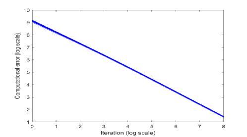
Figure C.1: Log-log plot of optimization error v.s. number of iterations: mirror descent for IS divergence minimization with 50 random starting points. All error curves are bounded above by the dashed line which has slope $-1$.

$\bullet$ DC programming for capped-$\ell_{1}$ SVM

High-dimensional classification with concurrent feature selection can be achieved by minimizing a composite objective function. Given $\boldsymbol{X}=[\boldsymbol{x}_{1},\ldots,\boldsymbol{x}_{n}]^{\top}\in\mathbb{R}^{n\times p}$ and $\boldsymbol{y}\in\{-1,1\}^{n}$, let $l(\boldsymbol{\beta})=\sum_{i=1}^{n}(1-y_{i}\boldsymbol{x}_{i}^{\top}\boldsymbol{\beta})_{+}$ be the hinge loss [61] that is nondifferentiable, and $P(\boldsymbol{\beta};\lambda)=\sum_{j=1}^{p}\min(\lambda|\beta_{j}|,\lambda^{2}/2)$ be the capped-$\ell_{1}$ penalty [66] which is nonsmooth and nonconvex. [42] proposed an effective DC algorithm for solving $\min_{\boldsymbol{\beta}}f(\boldsymbol{\beta}):=l(\boldsymbol{\beta})+P(\boldsymbol{\beta};\lambda)$ based on the decomposition $P(\boldsymbol{\beta};\lambda)=d_{1}(\boldsymbol{\beta};\lambda)-d_{2}(\boldsymbol{\beta};\lambda)$ with

$$d_{1}(\boldsymbol{\beta};\lambda)=\lambda\|\boldsymbol{\beta}\|_{1},~{}~{}d_{2}(\boldsymbol{\beta};\lambda)=\sum_{j=1}^{p}\max(\lambda|\beta_{j}|-\lambda^{2}/2,0).$$ (C.2)

As stated in Example 4, we can recharacterize DC as a Bregman-surrogate algorithm

$$\boldsymbol{\beta}^{(t+1)} \in\mathop{\arg\min}f(\boldsymbol{\beta})+\boldsymbol{\Delta}_{d_{2}}(\boldsymbol{\beta},\boldsymbol{\beta}^{(t)})$$ (C.3a)

$$\in\mathop{\arg\min}_{\boldsymbol{\beta}}\sum_{i=1}^{n}\max(0,1-y_{i}\boldsymbol{x}_{i}^{\top}\boldsymbol{\beta})+\lambda\sum_{j=1}^{p}\big{(}|\beta_{j}|-\beta_{j}1_{|\beta_{j}^{(t)}|\geq\lambda/2}\big{)}.$$ (C.3b)

(C.3b) is equivalent to a linear program: $\min_{\boldsymbol{\xi},\boldsymbol{\zeta},\boldsymbol{\beta}}\sum_{i=1}^{n}\xi_{i}+\lambda\sum_{j=1}^{p}\zeta_{j}-\lambda\sum_{j=1}^{p}\beta_{j}1_{|\beta_{j}^{(t)}|\geq\lambda/2}$ s.t. $\xi_{i}\geq 1-y_{i}\boldsymbol{x}_{i}^{\top}\boldsymbol{\beta}$ for $i\in[n]$, $-\zeta_{j}\leq\beta_{j}\leq\zeta_{j}$ for $j\in[p]$ and $\xi_{i},\zeta_{j}\geq 0$ for $i\in[n],j\in[p]$, which can be efficiently solved by standard linear programming (LP) solvers. For the convergence of the DC algorithm, a similar result can be shown for the optimization error $\mathrm{avg}_{0\leq t\leq T}(\boldsymbol{\Delta}_{l}+\mathrel{\mathop{\boldsymbol{\Delta}}\limits^{\vbox to0.0pt{\kern-2.0pt\hbox{$\scriptstyle\smallsetminus$}\vss}}}_{d_{2}}+\boldsymbol{\Delta}_{d_{1}})(\boldsymbol{\beta}^{(t)},\boldsymbol{\beta}^{(t+1)})$, following the lines of the proof of Proposition 4.

We generated $\boldsymbol{X}\in\mathbb{R}^{400\times 800}$ with each row following $\mathcal{N}(\boldsymbol{0},\boldsymbol{\Sigma})$ and $\Sigma_{ij}=0.5^{|i-j|}$, $\boldsymbol{\beta}^{*}=[15,10,0,\ldots,0]^{\top}$, and $\boldsymbol{y}=\mathrm{sgn}(\boldsymbol{X}\boldsymbol{\beta}^{*}+\boldsymbol{e})$ where $e_{i}\sim\mathcal{N}(0,\sigma^{2})$ with $\sigma^{2}=10$. We fixed $\lambda=1$ and ran the DC algorithm for 50 different starting points with each component randomly drawn from $U(0,1)$. The corresponding optimization error curves are plotted in Figure C.2, where the $\mathcal{O}(1/T)$ rate of convergence is impressive.

Figure C.2: Log-log plot of optimization error v.s. number of iterations: DC programming for capped-$\ell_{1}$ SVM (50 different initial points).

C.2 Statistical error

In this part, we consider two algorithms for sparse regression: LLA and iterative thresholding. The nonconvex “hard” penalty defined by (55) is applied, which is constructed from the hard-thresholding rule via (48). Given $\boldsymbol{X}\in\mathbb{R}^{n\times p}$ and $\boldsymbol{y}\in\mathbb{R}^{n}$, we study the following regularized problem $\min_{\boldsymbol{\beta}}f(\boldsymbol{\beta}):=l(\boldsymbol{\beta})+\sum_{j=1}^{p}P_{H}(\varrho\beta_{j};\lambda)$, where $l$ is the loss function and $\varrho=\|\boldsymbol{X}\|_{2}$. The loss functions under consideration are the ordinary quadratic loss and a nonconvex loss which is resistant to gross outliers:

• $\ell_{2}$ loss: $l(\boldsymbol{\beta})=\|\boldsymbol{y}-\boldsymbol{X}\boldsymbol{\beta}\|_{2}^{2}/2$;

• Tukey’s biweight loss: $l(\boldsymbol{\beta})=\sum_{i=1}^{n}\int_{0}^{|\boldsymbol{x}_{i}^{\top}\boldsymbol{\beta}-y_{i}|}\psi(t)\text{d}t$ and $\psi(t)=t[1-(t/c)^{2}]^{2}$ if $|t|\leq c$ and $0$ otherwise, where $c=4.685\sigma$ with $\sigma$ a robust estimate of the standard deviation of errors [26].

In either case, we have a nonconvex optimization problem. In simulations, the design matrix $\boldsymbol{X}\in\mathbb{R}^{n\times p}$ has i.i.d. rows drawn from $\mathcal{N}(\boldsymbol{0},\boldsymbol{\Sigma})$ with $\Sigma_{ij}=0.15^{|i-j|}$, the response is given by $\boldsymbol{y}=\boldsymbol{X}\boldsymbol{\beta}^{*}+\boldsymbol{e}$ with $e_{i}\sim N(0,\sigma^{2})$ and $\sigma^{2}=10$, and the regularization parameter $\lambda$ is set to $A\sigma\sqrt{\log(ep)}$. We set $n=800,p=1000,\boldsymbol{\beta}^{*}=[12,8,0,\ldots,0]^{\top}$ and $A=2$.

First, we tested the statistical accuracy of LLA (cf. Theorem 3 and Proposition 5). We generated 15 initial points $\boldsymbol{\beta}^{(0)}$ with each element following $U(-a,a)$, with $a\in\{0.5,1,1.5\}$ and 5 for each. Figure C.3 shows how the statistical error varies as the cycles progress, with each curve representing an average over 20 implementations of the same setting. Here, the errors are plotted on a log scale for a better view of the convergence rate. Unlike Figure C.1 and Figure C.2, the statistical errors can not reach 0 (or $-\infty$ in the log plot) due to the existence of noise. But they all achieved essentially the same order of statistical precision, which verifies Theorem 3, and the statistical convergence of LLA was really fast.

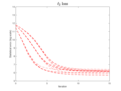
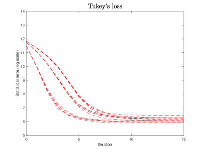
Figure C.3: Log plot of the statistical accuracy of LLA iterates in $P_{H}$-penalized sparse regression (left) and robust regression (right).

On the other hand, the computational burden of LLA turned out to be pretty high, mainly due to the cost of solving a weighted lasso problem at each iteration. We thus turned to iterative thresholding because of its low per-iteration complexity. Figure C.4 shows some analogous results. According to Figure C.4, all final statistical errors were controlled within the same order of precision. The convergence process seems to conform to the bound in Theorem 5: when $t$ is small, $\log\boldsymbol{\Delta}_{\psi}(\boldsymbol{\beta}^{*},\boldsymbol{\beta}^{(t)})\lesssim-\log(1/\kappa)\,t+\log(\boldsymbol{\Delta}_{\psi}(\boldsymbol{\beta}^{*},\boldsymbol{\beta}^{(0)}))$, and when $t$ is large, $\log\boldsymbol{\Delta}_{\psi}(\boldsymbol{\beta}^{*},\boldsymbol{\beta}^{(t)})\lesssim\kappa^{t}\boldsymbol{\Delta}_{\psi}(\boldsymbol{\beta}^{*},\boldsymbol{\beta}^{(0)})+\log(\kappa K\lambda^{2}J^{*}/(1-\kappa))$, demonstrating an exponential decay.

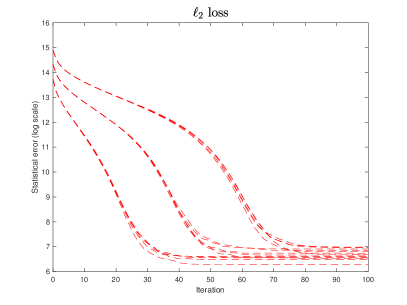
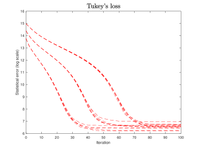
Figure C.4: Log plot of the statistical accuracy of iterative thresholding iterates in $P_{H}$-penalized sparse regression (left) and robust regression (right).

C.3 Accelerations

We test the acceleration schemes in IS divergence minimization and robust sparse regression in this subsection.

Figure C.5 shows the power of applying the (second) acceleration in IS divergence minimization problem in Section C.1, where we used 50 starting points with $\beta_{j}^{(0)}\sim U(0,1),1\leq j\leq p$. With the acceleration, the number of iterations was brought down from 1000 to less than 50 to reach the same value of the objective function, and the overall computational time was saved by nearly 90%.

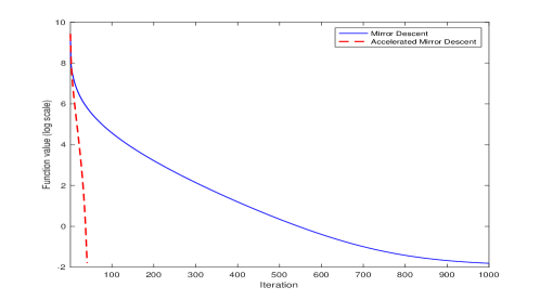
Figure C.5: Objective function value (shown on $\log$ scale) v.s. number of iterations for the plain and accelerated exponentiated gradient descent algorithms in nonconvex Burg entropy optimization.

Figure C.6 shows the convergence of statistical error when applying the (first) acceleration scheme in iterative thresholding for the $P_{H}$-penalized Tukey’s loss minimization problem as mentioned in Section C.2. The simulation setting remains the same as before and we sampled 20 initial points with $\beta_{j}^{(0)}\sim U(-1,1),1\leq j\leq p$. A substantial reduction in the number of iterations was achieved. Of course, the line search causes some overhead in computation. But the accelerated iterative thresholding still reduced the overall running time by more than 30%, and obtained slightly better statistical accuracy.

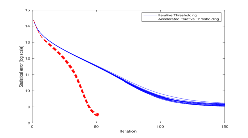
Figure C.6: Statistical error (shown on $\log$ scale) v.s. iteration number for iterative thresholding and accelerated iterative thresholding in robust sparse regression.

References

- [1] {barticle}[author] \bauthor\bsnmAgarwal, \bfnmAlekh\binitsA., \bauthor\bsnmNegahban, \bfnmSahand\binitsS. and \bauthor\bsnmWainwright, \bfnmMartin J.\binitsM. J. (\byear2012). \btitleFast global convergence of gradient methods for high-dimensional statistical recovery. \bjournalThe Annals of Statistics \bvolume40 \bpages2452–2482. \endbibitem
- [2] {barticle}[author] \bauthor\bsnmAn, \bfnmLe Thi Hoai\binitsL. T. H. and \bauthor\bsnmTao, \bfnmPham Dinh\binitsP. D. (\byear2005). \btitleThe DC (difference of convex functions) programming and DCA revisited with DC models of real world nonconvex optimization problems. \bjournalAnnals of Operations Research \bvolume133 \bpages23–46. \endbibitem
- [3] {barticle}[author] \bauthor\bsnmBanerjee, \bfnmArindam\binitsA., \bauthor\bsnmMerugu, \bfnmSrujana\binitsS., \bauthor\bsnmDhillon, \bfnmInderjit S.\binitsI. S. and \bauthor\bsnmGhosh, \bfnmJoydeep\binitsJ. (\byear2005). \btitleClustering with Bregman Divergences. \bjournalJournal of Machine Learning Research (JMLR) \bvolume6. \endbibitem
- [4] {barticle}[author] \bauthor\bsnmBeck, \bfnmAmir\binitsA. and \bauthor\bsnmTeboulle, \bfnmMarc\binitsM. (\byear2009). \btitleA fast iterative shrinkage-thresholding algorithm for linear inverse problems. \bjournalSIAM Journal on Imaging Sciences \bvolume2 \bpages183–202. \endbibitem
- [5] {bmisc}[author] \bauthor\bsnmBen-Tal, \bfnmA.\binitsA. and \bauthor\bsnmNemirovski, \bfnmA.\binitsA. (\byear2013). \btitleOptimization III: Convex Analysis, Nonlinear Programming Theory, Standard Nonlinear Programming Algorithms. \bhowpublishedLecture Notes. \endbibitem
- [6] {bbook}[author] \bauthor\bsnmBertsekas, \bfnmDimitri P.\binitsD. P. (\byear1999). \btitleNonlinear Programming, \bedition2nd ed. \bpublisherAthena Scientific. \endbibitem
- [7] {barticle}[author] \bauthor\bsnmBickel, \bfnmPeter J\binitsP. J., \bauthor\bsnmRitov, \bfnmYa’acov\binitsY. and \bauthor\bsnmTsybakov, \bfnmAlexandre B\binitsA. B. (\byear2009). \btitleSimultaneous analysis of lasso and Dantzig selector. \bjournalThe Annals of Statistics \bpages1705–1732. \endbibitem
- [8] {barticle}[author] \bauthor\bsnmBlumensath, \bfnmT.\binitsT. and \bauthor\bsnmDavies, \bfnmM. E.\binitsM. E. (\byear2009). \btitleIterative hard thresholding for compressed sensing. \bjournalApplied and Computational Harmonic Analysis \bvolume27 \bpages265–274. \endbibitem
- [9] {barticle}[author] \bauthor\bsnmBregman, \bfnmL. M.\binitsL. M. (\byear1967). \btitleThe relaxation method of finding the common point of convex sets and its application to the solution of problems in convex programming. \bjournalUSSR Computational Mathematics and Mathematical Physics \bvolume7 \bpages200–217. \endbibitem
- [10] {barticle}[author] \bauthor\bsnmBunea, \bfnmFlorentina\binitsF., \bauthor\bsnmTsybakov, \bfnmAlexandre\binitsA. and \bauthor\bsnmWegkamp, \bfnmMarten\binitsM. (\byear2007). \btitleSparsity oracle inequalities for the LASSO. \bjournalElectronic Journal of Statistics \bvolume1 \bpages169–194. \endbibitem
- [11] {barticle}[author] \bauthor\bsnmCandes, \bfnmEmmanuel\binitsE. and \bauthor\bsnmTao, \bfnmTerence\binitsT. (\byear2007). \btitleThe Dantzig selector: Satistical estimation when p is much larger than n. \bjournalThe Annals of Statistics \bpages2313–2351. \endbibitem
- [12] {barticle}[author] \bauthor\bsnmCandes, \bfnmE. J.\binitsE. J. and \bauthor\bsnmTao, \bfnmT.\binitsT. (\byear2005). \btitleDecoding by Linear Programming. \bjournalIEEE Trans. Inf. Theor. \bvolume51 \bpages4203–4215. \endbibitem
- [13] {barticle}[author] \bauthor\bsnmCao, \bauthor\bsnmEggermont, \bfnmPaul P. B.\binitsP. P. B. and \bauthor\bsnmTerebey, \bfnmSusan\binitsS. (\byear1999). \btitleCross Burg entropy maximization and its application to ringing suppression in image reconstruction. \bjournalIEEE Transactions on Image Processing \bvolume8 \bpages286–292. \endbibitem
- [14] {barticle}[author] \bauthor\bsnmChen, \bfnmGong\binitsG. and \bauthor\bsnmTeboulle, \bfnmMarc\binitsM. (\byear1993). \btitleConvergence Analysis of a Proximal-Like Minimization Algorithm Using Bregman Functions. \bjournalSIAM Journal on Optimization \bvolume3 \bpages538–543. \endbibitem
- [15] {binproceedings}[author] \bauthor\bsnmCichocki, \bfnmAndrzej\binitsA., \bauthor\bparticleichi \bsnmAmari, \bfnmShun\binitsS., \bauthor\bsnmZdunek, \bfnmRafal\binitsR., \bauthor\bsnmKompass, \bfnmRaul\binitsR., \bauthor\bsnmHori, \bfnmGen\binitsG. and \bauthor\bsnmHe, \bfnmZhaoshui\binitsZ. (\byear2006). \btitleExtended SMART algorithms for non-negative matrix factorization. In \bbooktitleICAISC (\beditor\bfnmLeszek\binitsL. \bsnmRutkowski, \beditor\bfnmRyszard\binitsR. \bsnmTadeusiewicz, \beditor\bfnmLotfi A.\binitsL. A. \bsnmZadeh and \beditor\bfnmJacek M.\binitsJ. M. \bsnmZurada, eds.). \bseriesLecture Notes in Computer Science \bvolume4029 \bpages548-562. \bpublisherSpringer. \endbibitem
- [16] {barticle}[author] \bauthor\bsnmCorrea, \bfnmR.\binitsR., \bauthor\bsnmJofre, \bfnmA.\binitsA. and \bauthor\bsnmThibault, \bfnmT.\binitsT. (\byear1994). \btitleSubdifferential Monotonicity as Characterization of Convex Functions. \bjournalNumerical Functional Analysis and Optimization \bvolume15 \bpages531–535. \endbibitem
- [17] {barticle}[author] \bauthor\bsnmDonoho, \bfnmD.\binitsD. and \bauthor\bsnmJohnstone, \bfnmI.\binitsI. (\byear1994). \btitleIdeal Spatial Adaptation via Wavelet Shrinkages. \bjournalBiometrika \bvolume81 \bpages425–455. \endbibitem
- [18] {barticle}[author] \bauthor\bsnmDuchi, \bfnmJohn C.\binitsJ. C., \bauthor\bsnmHazan, \bfnmElad\binitsE. and \bauthor\bsnmSinger, \bfnmY.\binitsY. (\byear2011). \btitleAdaptive Subgradient Methods for Online Learning and Stochastic Optimization. \bjournalJ. Mach. Learn. Res. \bvolume12 \bpages2121-2159. \endbibitem
- [19] {barticle}[author] \bauthor\bsnmFan, \bfnmJ.\binitsJ. and \bauthor\bsnmLi, \bfnmR.\binitsR. (\byear2001). \btitleVariable selection via nonconcave penalized likelihood and its oracle properties. \bjournalJournal of the American Statistical Association \bvolume96 \bpages1348–1360. \endbibitem
- [20] {barticle}[author] \bauthor\bsnmFan, \bfnmJianqing\binitsJ., \bauthor\bsnmXue, \bfnmLingzhou\binitsL. and \bauthor\bsnmZou, \bfnmHui\binitsH. (\byear2014). \btitleStrong oracle optimality of folded concave penalized estimation. \bjournalThe Annals of Statistics \bvolume42 \bpages819–849. \endbibitem
- [21] {barticle}[author] \bauthor\bsnmFévotte, \bfnmCédric\binitsC., \bauthor\bsnmBertin, \bfnmNancy\binitsN. and \bauthor\bsnmDurrieu, \bfnmJean-Louis\binitsJ.-L. (\byear2009). \btitleNonnegative Matrix Factorization with the Itakura-saito Divergence: With Application to Music Analysis. \bjournalNeural Computation \bvolume21 \bpages793–830. \endbibitem
- [22] {barticle}[author] \bauthor\bsnmFrank, \bfnmIldiko E.\binitsI. E. and \bauthor\bsnmFriedman, \bfnmJerome H.\binitsJ. H. (\byear1993). \btitleA Statistical View of Some Chemometrics Regression Tools. \bjournalTechnometrics \bvolume35 \bpages109-135. \endbibitem
- [23] {barticle}[author] \bauthor\bsnmGasso, \bfnmGilles\binitsG., \bauthor\bsnmRakotomamonjy, \bfnmAlain\binitsA. and \bauthor\bsnmCanu, \bfnmSt phane\binitsS. (\byear2009). \btitleRecovering sparse signals with a certain family of nonconvex penalties and DC programming. \bjournalIEEE Transactions on Signal Processing \bvolume57 \bpages4686-4698. \endbibitem
- [24] {barticle}[author] \bauthor\bsnmGhadimi, \bfnmSaeed\binitsS. and \bauthor\bsnmLan, \bfnmGuanghui\binitsG. (\byear2016). \btitleAccelerated gradient methods for nonconvex nonlinear and stochastic programming. \bjournalMathematical Programming \bvolume156 \bpages59–99. \endbibitem
- [25] {barticle}[author] \bauthor\bsnmHagood, \bfnmJohn W.\binitsJ. W. and \bauthor\bsnmThomson, \bfnmBrian S.\binitsB. S. (\byear2006). \btitleRecovering a function from a Dini derivative. \bjournalThe American Mathematical Monthly \bvolume113 \bpages34-46. \endbibitem
- [26] {bbook}[author] \bauthor\bsnmHampel, \bfnmFrank R.\binitsF. R., \bauthor\bsnmRonchetti, \bfnmElvezio M.\binitsE. M., \bauthor\bsnmRousseeuw, \bfnmPeter J.\binitsP. J. and \bauthor\bsnmStahel, \bfnmWerner A.\binitsW. A. (\byear2005). \btitleRobust Statistics. \bpublisherJohn Wiley & Sons, New York. \endbibitem
- [27] {bbook}[author] \bauthor\bsnmHuber, \bfnmPeter J.\binitsP. J. (\byear1981). \btitleRobust Statistics. \bpublisherJohn Wiley and Sons, \baddressNew York. \endbibitem
- [28] {barticle}[author] \bauthor\bsnmHunter, \bfnmDavid R.\binitsD. R. and \bauthor\bsnmLange, \bfnmKenneth\binitsK. (\byear2004). \btitleA tutorial on MM algorithms. \bjournalThe American Statistician \bpages30–37. \endbibitem
- [29] {barticle}[author] \bauthor\bsnmHunter, \bfnmDavid R.\binitsD. R. and \bauthor\bsnmLi, \bfnmRunze\binitsR. (\byear2005). \btitleVariable selection using MM algorithms. \bjournalThe Annals of Statistics \bvolume33 \bpages1617–1642. \bdoi10.1214/009053605000000200 \endbibitem
- [30] {barticle}[author] \bauthor\bsnmJørgensen, \bfnmBent\binitsB. (\byear1987). \btitleExponential Dispersion Models. \bjournalJournal of the Royal Statistical Society. Series B \bvolume49 \bpages127-145. \endbibitem
- [31] {bbook}[author] \bauthor\bsnmKoltchinskii, \bfnmVladimir\binitsV. (\byear2011). \btitleOracle Inequalities in Empirical Risk Minimization and Sparse Recovery Problems. \bpublisherSpringer. \endbibitem
- [32] {binproceedings}[author] \bauthor\bsnmKrichene, \bfnmWalid\binitsW., \bauthor\bsnmBayen, \bfnmAlexandre\binitsA. and \bauthor\bsnmBartlett, \bfnmPeter L\binitsP. L. (\byear2015). \btitleAccelerated Mirror Descent in Continuous and Discrete Time. In \bbooktitleAdvances in Neural Information Processing Systems (\beditor\bfnmC.\binitsC. \bsnmCortes, \beditor\bfnmN.\binitsN. \bsnmLawrence, \beditor\bfnmD.\binitsD. \bsnmLee, \beditor\bfnmM.\binitsM. \bsnmSugiyama and \beditor\bfnmR.\binitsR. \bsnmGarnett, eds.) \bvolume28. \bpublisherCurran Associates, Inc. \endbibitem
- [33] {barticle}[author] \bauthor\bsnmLange, \bfnmKenneth\binitsK. and \bauthor\bsnmZhou, \bfnmHua\binitsH. (\byear2014). \btitleMM algorithms for geometric and signomial programming. \bjournalMathematical Programming \bvolume143 \bpages339–356. \endbibitem
- [34] {barticle}[author] \bauthor\bsnmLee, \bfnmDaniel D.\binitsD. D. and \bauthor\bsnmSeung, \bfnmH. Sebastian\binitsH. S. (\byear1999). \btitleLearning the parts of objects by nonnegative matrix factorization. \bjournalNature \bvolume401 \bpages788–791. \endbibitem
- [35] {binproceedings}[author] \bauthor\bsnmLefèvre, \bfnmAugustin\binitsA., \bauthor\bsnmBach, \bfnmFrancis R.\binitsF. R. and \bauthor\bsnmFévotte, \bfnmCédric\binitsC. (\byear2011). \btitleOnline algorithms for nonnegative matrix factorization with the Itakura-Saito divergence. In \bbooktitleIEEE Workshop on Applications of Signal Processing to Audio and Acoustics, WASPAA 2011 \bpages313–316. \endbibitem
- [36] {barticle}[author] \bauthor\bsnmLoh, \bfnmPo-Ling\binitsP.-L. and \bauthor\bsnmWainwright, \bfnmMartin J.\binitsM. J. (\byear2015). \btitleRegularized M-estimators with nonconvexity: statistical and algorithmic theory for local optima. \bjournalJournal Machine Learning Research \bvolume16 \bpages559–616. \endbibitem
- [37] {barticle}[author] \bauthor\bsnmLounici, \bfnmKarim\binitsK., \bauthor\bsnmPontil, \bfnmMassimiliano\binitsM., \bauthor\bsnmTsybakov, \bfnmAlexandre B.\binitsA. B. and \bauthor\bsnmvan de Geer, \bfnmSara\binitsS. (\byear2011). \btitleOracle Inequalities and Optimal Inference under Group Sparsity. \bjournalAnnals of Statistics \bvolume39 \bpages2164-2204. \endbibitem
- [38] {bbook}[author] \bauthor\bsnmNemirovski, \bfnmA.\binitsA. and \bauthor\bsnmYudin, \bfnmD.\binitsD. (\byear1983). \btitleProblem complexity and method efficiency in optimization. \bseriesWiley-Interscience series in discrete mathematics. \bpublisherWiley, \baddressChichester, New York. \endbibitem
- [39] {barticle}[author] \bauthor\bsnmNesterov, \bfnmYurii\binitsY. (\byear1983). \btitleA method of solving a convex programming problem with convergence rate . \bjournalSoviet Mathematics Doklady \bvolume27 \bpages372–376. \endbibitem
- [40] {barticle}[author] \bauthor\bsnmNesterov, \bfnmYurii\binitsY. (\byear1988). \btitleOn an approach to the construction of optimal methods of minimization of smooth convex functions. \bjournalEkonom. i. Mat. Metody (In Russian) \bvolume24 \bpages509–517. \endbibitem
- [41] {bbook}[author] \bauthor\bsnmNesterov, \bfnmYurii\binitsY. (\byear2004). \btitleIntroductory Lectures on Convex Optimization: A Basic Course. \bseriesApplied optimization. \bpublisherKluwer Academic Publ., \baddressBoston, Dordrecht, London. \endbibitem
- [42] {barticle}[author] \bauthor\bsnmOng, \bfnmCheng Soon\binitsC. S. and \bauthor\bsnmAn, \bfnmLe Thi Hoai\binitsL. T. H. (\byear2013). \btitleLearning sparse classifiers with difference of convex functions algorithms. \bjournalOptimization Methods and Software \bvolume28 \bpages830-854. \endbibitem
- [43] {barticle}[author] \bauthor\bsnmPan, \bfnmWei\binitsW., \bauthor\bsnmShen, \bfnmXiaotong\binitsX. and \bauthor\bsnmLiu, \bfnmBinghui\binitsB. (\byear2013). \btitleCluster analysis: unsupervised learning via supervised learning with a non-convex penalty. \bjournalJournal of Machine Learning Research \bvolume14 \bpages1865–1889. \endbibitem
- [44] {barticle}[author] \bauthor\bsnmRigollet, \bfnmPhilippe\binitsP. and \bauthor\bsnmTsybakov, \bfnmAlexandre\binitsA. (\byear2011). \btitleExponential Screening and optimal rates of sparse estimation. \bjournalAnnals of Statistics \bvolume39 \bpages731–771. \endbibitem
- [45] {bbook}[author] \bauthor\bsnmRockafellar, \bfnmR. Tyrrell\binitsR. T. (\byear1970). \btitleConvex Analysis. \bpublisherPrinceton University Press, \baddressPrinceton, NJ. \endbibitem
- [46] {bphdthesis}[author] \bauthor\bsnmSchmidt, \bfnmMark\binitsM. (\byear2010). \btitleGraphical Model Structure Learning with -Regularization, \btypePhD thesis, \bpublisherUniversity of British Columbia. \endbibitem
- [47] {barticle}[author] \bauthor\bsnmShe, \bfnmYiyuan\binitsY. (\byear2009). \btitleThresholding-based Iterative Selection Procedures for Model Selection and Shrinkage. \bjournalElectronic Journal of Statistics \bvolume3 \bpages384-415. \endbibitem
- [48] {barticle}[author] \bauthor\bsnmShe, \bfnmYiyuan\binitsY. (\byear2012). \btitleAn iterative algorithm for fitting nonconvex penalized generalized linear models with grouped predictors. \bjournalComputational Statistics and Data Analysis \bvolume9 \bpages2976-2990. \endbibitem
- [49] {barticle}[author] \bauthor\bsnmShe, \bfnmYiyuan\binitsY. (\byear2016). \btitleOn the finite-sample analysis of -estimators. \bjournalElectronic Journal of Statistics \bvolume10 \bpages1874–1895. \bdoi10.1214/15-EJS1100 \endbibitem
- [50] {barticle}[author] \bauthor\bsnmShe, \bfnmY.\binitsY. and \bauthor\bsnmChen, \bfnmK.\binitsK. (\byear2017). \btitleRobust reduced-rank regression. \bjournalBiometrika \bvolume104 \bpages633-647. \endbibitem
- [51] {barticle}[author] \bauthor\bsnmShe, \bfnmYiyuan\binitsY., \bauthor\bsnmHe, \bfnmYuejia\binitsY. and \bauthor\bsnmWu, \bfnmDapeng\binitsD. (\byear2014). \btitleLearning Topology and Dynamics of Large Recurrent Neural Networks. \bjournalIEEE Transactions on Signal Processing \bvolume62 \bpages5881-5891. \endbibitem
- [52] {barticle}[author] \bauthor\bsnmShe, \bfnmYiyuan\binitsY., \bauthor\bsnmLi, \bfnmHuanghuang\binitsH., \bauthor\bsnmWang, \bfnmJiangping\binitsJ. and \bauthor\bsnmWu, \bfnmDapeng\binitsD. (\byear2013). \btitleGrouped Iterative Spectrum Thresholding for Super-Resolution Sparse Spectrum Selection. \bjournalIEEE Transactions on Signal Processing \bvolume61 \bpages6371-6386. \endbibitem
- [53] {barticle}[author] \bauthor\bsnmShe, \bfnmY.\binitsY., \bauthor\bsnmShen, \bfnmJ.\binitsJ. and \bauthor\bsnmZhang, \bfnmC.\binitsC. \btitleSupervised Multivariate Learning with Simultaneous Feature Auto-grouping and Dimension Reduction. \bjournalJournal of the Royal Statistical Society: Series B (Statistical Methodology). \bnoteTo appear. \endbibitem
- [54] {barticle}[author] \bauthor\bsnmShe, \bfnmY.\binitsY., \bauthor\bsnmWang, \bfnmZ.\binitsZ. and \bauthor\bsnmShen, \bfnmJ.\binitsJ. \btitle Gaining Outlier Resistance with Progressive Quantiles: Fast Algorithms and Theoretical Studies. \bjournalJournal of the American Statistical Association. \bnoteTo appear. \endbibitem
- [55] {barticle}[author] \bauthor\bsnmTao, \bfnmPham Dinh\binitsP. D. and \bauthor\bsnmSouad, \bfnmE. B.\binitsE. B. (\byear1986). \btitleAlgorithms for solving a class of nonconvex optimization problems. Methods of subgradients. \bjournalNorth-Holland Mathematics Studies \bvolume129 \bpages249-271. \endbibitem
- [56] {barticle}[author] \bauthor\bsnmTibshirani, \bfnmR.\binitsR. (\byear1996). \btitleRegression Shrinkage and Selection via the Lasso. \bjournalJournal of the Royal Statistical Society (Series B) \bvolume58 \bpages267-288. \endbibitem
- [57] {barticle}[author] \bauthor\bsnmTseng, \bfnmPaul\binitsP. (\byear2008). \btitleOn accelerated proximal gradient methods for convex-concave optimization. \bpagesTechnical report, Department of Mathematics, University of Washington. \endbibitem
- [58] {bbook}[author] \bauthor\bsnmTsybakov, \bfnmAlexandre B.\binitsA. B. (\byear2008). \btitleIntroduction to Nonparametric Estimation. \bpublisherSpringer, \baddressNew York, NY. \endbibitem
- [59] {barticle}[author] \bauthor\bparticlevan de \bsnmGeer, \bfnmSara A\binitsS. A. and \bauthor\bsnmBühlmann, \bfnmPeter\binitsP. (\byear2009). \btitleOn the conditions used to prove oracle results for the Lasso. \bjournalElectronic Journal of Statistics \bvolume3 \bpages1360–1392. \endbibitem
- [60] {bbook}[author] \bauthor\bparticlevan der \bsnmVaart, \bfnmA. W.\binitsA. W. and \bauthor\bsnmWellner, \bfnmJ.\binitsJ. (\byear1996). \btitleWeak Convergence and Empirical Processes: With Applications to Statistics. \bpublisherSpringer. \endbibitem
- [61] {bbook}[author] \bauthor\bsnmVapnik, \bfnmVladimir N.\binitsV. N. (\byear1995). \btitleThe Nature of Statistical Learning Theory. \bpublisherSpringer-Verlag, \baddressNew York, NY, USA. \endbibitem
- [62] {barticle}[author] \bauthor\bsnmWainwright, \bfnmMartin J.\binitsM. J. and \bauthor\bsnmJordan, \bfnmMichael I.\binitsM. I. (\byear2008). \btitleGraphical Models, Exponential Families, and Variational Inference. \bjournalFoundations and Trends in Machine Learning \bvolume1 \bpages1-305. \endbibitem
- [63] {barticle}[author] \bauthor\bsnmWang, \bfnmZhaoran\binitsZ., \bauthor\bsnmLiu, \bfnmHan\binitsH. and \bauthor\bsnmZhang, \bfnmTong\binitsT. (\byear2014). \btitleOptimal computational and statistical rates of convergence for sparse nonconvex learning problems. \bjournalThe Annals of Statistics \bvolume42 \bpages2164–2201. \endbibitem
- [64] {barticle}[author] \bauthor\bsnmZhang, \bfnmChunming\binitsC., \bauthor\bsnmJiang, \bfnmYuan\binitsY. and \bauthor\bsnmChai, \bfnmYi\binitsY. (\byear2010). \btitlePenalized Bregman divergence for large-dimensional regression and classification. \bjournalBiometrika \bvolume97 \bpages551–566. \endbibitem
- [65] {barticle}[author] \bauthor\bsnmZhang, \bfnmC. H.\binitsC. H. (\byear2010). \btitleNearly unbiased variable selection under minimax concave penalty. \bjournalThe Annals of Statistics \bvolume38 \bpages894-942. \endbibitem
- [66] {barticle}[author] \bauthor\bsnmZhang, \bfnmTong\binitsT. (\byear2010). \btitleAnalysis of Multi-stage Convex Relaxation for Sparse Regularization. \bjournalJournal of Machine Learning Research \bvolume11 \bpages1081–1107. \endbibitem
- [67] {barticle}[author] \bauthor\bsnmZou, \bfnmH.\binitsH. and \bauthor\bsnmLi, \bfnmR.\binitsR. (\byear2008). \btitleOne-step Sparse Estimates in Nonconcave Penalized Likelihood Models. \bjournalAnnals of Statistics \bvolume36 \bpages1509–1533. \endbibitem