Study of the Very High Energy emission of M87 through its broadband spectral energy distribution

Abstract

The radio galaxy M87 is the central dominant galaxy of the Virgo Cluster. Very High Energy (VHE,$\gtrsim 0.1$ TeV) emission, from M87 has been detected by Imaging Air Cherenkov Telescopes (IACTs ). Recently, marginal evidence for VHE long-term emission has also been observed by the High Altitude Water Cherenkov (HAWC) Observatory, a gamma ray and cosmic-ray detector array located in Puebla, Mexico. The mechanism that produces VHE emission in M87 remains unclear. This emission is originated in its prominent jet, which has been spatially resolved from radio to X-rays. In this paper, we constructed a spectral energy distribution from radio to gamma rays that is representative of the non-flaring activity of the source, and in order to explain the observed emission, we fit it with a lepto-hadronic emission model. We found that this model is able to explain non-flaring VHE emission of M87 as well as an orphan flare reported in 2005.

1 Introduction

Gamma rays constitute the highest energy electromagnetic radiation tracing the most energetic phenomena in the Universe. Active Galactic Nuclei (AGN) are important sources of extragalactic gamma rays, and according to the current consensus they are powered by accreting super massive black holes (SMBH). Most AGNs that are VHE emitters are classified as blazars, i.e. radio-loud AGNs whose jets are pointing nearly towards the observer. Since particles within the jet travel at nearly the speed of light, relativistic beaming increases the brightness of these objects. According to unification schemes (Urry & Padovani, 1995), radio galaxies (RDGs) correspond to the misaligned counterparts of blazars, and so far, VHE emission has been detected from six of them (Rieger & Levinson, 2018). Since RDGs are located on average closer than blazars, it is possible obtain more detailed observations to test theoretical models of their emission. The broadband spectral energy distributions (SED) of AGN jets, which are prominent in the emission of blazars and RDGs, are globally non thermal and they are characterized by the presence of two components (generally referred to as “peaks”) (Blandford et al., 2019). The low energy component is usually attributed to synchrotron emission, which is produced when relativistic particles are moving in the presence of a magnetic field (Rybicki & Lightman, 2008). On the other hand, the second peak has been explained by many different models. These models can be divided into two types: leptonic, where the high energy component of the broadband SED is explained as inverse Compton (IC) emission produced by an electron population in the jet (Longair, 2011), and hadronic, where the second component is produced by mechanisms involving the collision of accelerated protons with the surrounding environment (Mücke et al., 2003).

M87 (R.A. $12^{\text{h}}30^{\text{m}}47^{\text{s}}.2$ Dec.$+12^{\circ}23^{\prime}51^{\prime\prime}$), which is classified as a giant Fanaroff-Riley I (FR-I) RDG, is the central dominant galaxy of the Virgo Cluster. It is an elliptical galaxy with a diameter of $\sim$300 kpc (Doherty et al., 2009), a dynamical mass within 180 kpc estimated as $(1.5\pm 0.2)\times 10^{13}\ M_{\odot}$ (Zhu et al., 2014) and a redshift of $z=0.0044$. It is located at a distance of 16.4 $\pm$ 0.5 Mpc, which is a redshift independent measurement (Bird et al., 2010). M87 hosts a SMBH, named M87*, whose shadow was the first imaged by the Event Horizon Telescope (The EHT Collaboration et al., 2019). The prominent jet of M87 is one its most noticeable characteristics. This jet has been studied for the last one hundred years (Curtis, 1918), it has a length of about 2.5 kpc (Biretta et al., 1999) and has been resolved from radio to X-rays. It presents complex structures like knots and diffuse emission (Perlman et al., 1999, 2001), apparent superluminal motion (Cheung et al., 2007) and a complex variability (Harris et al., 2006).

M87 was the first RDG detected at VHE (Aharonian et al., 2003). It has been detected by different IACTs such as HESS (Aharonian et al., 2006), VERITAS (Acciari et al., 2010) and MAGIC. (Acciari et al., 2020) Recently, the HAWC Collaboration (Albert et al., 2021) reported weak evidence (3.6$\sigma$) of long-term VHE emission from this source. M87 has shown a complex behavior at VHE (Ait Benkhali et al., 2019) with a rapid variability during flaring states (Abramowski et al., 2012). According to available observations, three VHE flares from M87 have been detected in 2005 (Aharonian et al., 2006), 2008 (Albert et al., 2008) and 2010 (Abramowski et al., 2012). Gamma ray angular resolution is not sufficient to determine the region of the galaxy where this emission is produced. Variability studies have suggested that the innermost jet zone of M87 is most likely the source of its VHE emission. The other candidate location is the jet feature HST-1, but it is disfavored by the VHE timescale variability and the lack of correlated activity in other bands during TeV flares (Abramowski et al., 2012; Ait Benkhali et al., 2019).

The broadband emission of M87 has usually been explained by a one-zone Synchrotron Self Compton (SSC) scenario (Abdo et al., 2009; De Jong et al., 2015). In these models, the first component is attributed to synchrotron radiation that is produced by electrons moving at relativistic velocity with random orientation with respect to the magnetic field. The second peak is explained by inverse Compton scattering of synchrotron photons to higher energies by the same electron population. However, some authors claim that SSC models are not able to explain VHE emission in M87. Evidence for a possible spectral turnover in the GeV regime $E\gtrsim 10$ GeV was found by Ait Benkhali et al. (2019). This was interpreted as due to the presence of an additional physical component in the emission. However, constraining the decrease of this component from only Fermi data is not possible and long-term TeV observations are needed. One zone SSC models were found to have difficulties in explaining VHE/X-ray correlated variability in M87 (Abramowski et al., 2012), and Fraija & Marinelli (2016) claimed that one-zone SSC models cannot be extended to VHE in FR-I RDGs. This is why alternative ideas have been proposed to explain the SED such as seed photons coming from other regions in the jet (Georganopoulos et al., 2005) and photo-hadronic interactions (Fraija & Marinelli, 2016).

The main goal of this work is comparing the VHE emission of the RDG M87 observed by IACTs during specific epochs (including the 2005 flare) with the long term quiescent/average emission provided by continuous observation by the HAWC observatory from 2014 to 2019. We used a lepto-hadronic model, which combines SSC and photo-hadronic scenarios, to explain this emission. We developed a Python code to simulate the broadband emission of M87 and constructed an average SED of M87 collecting multifrequency observations from data archives. Preliminary results of this work were released in Ureña-Mena et al. (2021).

2 Data

We collected historical archive data to construct the broadband SED of M87. Data sets from radio to X-rays were partially based on those observations of the innermost jet zone used by Abdo et al. (2009), Fraija & Marinelli (2016) and Prieto et al. (2016). MeV-GeV gamma ray data were obtained from the Fermi Large Area Telescope Fourth Source Catalog (4FGL), which is based on the first eight years of data from the Fermi Gamma-ray Space Telescope (Abdollahi et al., 2020). The 4FGL covers an energy range from 50 MeV to 1 TeV. Four different sets of data were used for the TeV range: 1) H.E.S.S observations from 2004, which were taken during a TeV quiescent phase (Aharonian et al., 2006). 2) H.E.S.S observations from 2005, which were taken during a TeV high activity state but without evidence of inner jet activity in the rest of the broadband inner jet spectrum (Aharonian et al., 2006). That is why we use the same broadband SED as in the non-flaring state case. 3) MAGIC-I observations from 2005-2007, which correspond to an observation campaign where no flaring activity was detected (Aleksić et al., 2012). 4) HAWC observations, which cover a quiescent period from 2014 to 2019 corresponding to 1,523 days. (Albert et al., 2021).

The HAWC array consists of 300 water Cherenkov detectors (WCD), each with 4 photomultiplier tubes (PMT). The HAWC data is divided into nine bins according to the fraction of channels hit, which are used to estimate the energy of the events (see Abeysekara et al. (2017) for more details). In Albert et al. (2021) a power law spectrum, with a spectral index set to 2.5, was fit to a sample of 138 nearby AGN. For those sources with a $TS>9$, including M87, an optimized spectrum with free normalization and spectral index was obtained. Then, quasi differential flux limits were obtained in three bands: $0.5-2.0$ TeV, $2.0-8.0$ TeV and $8.0-32.0$ TeV.

3 Emission model

We used a hybrid model in this work. Emission components from radio to GeV gamma rays are explained with an SSC scenario whereas photo-hadronic interactions are added to explain the VHE emission. Therefore, the broadband SED has been modeled with three components. Due to the low redshift of the source, extragalactic background light (EBL) absorption was not relevant for photon energies $\lesssim 10$ TeV and we did not consider it in the modeling. HAWC data, which are the only data set affected by some relevant EBL absorption, were already corrected for this effect (Albert et al., 2021) using the EBL model of Domínguez et al. (2011). We used the one-zone SSC code described in Finke et al. (2008), which considers a homogeneous spherical region or blob in the inner jet moving with a Lorentz factor $\Gamma$ and a randomly oriented magnetic field with mean intensity $B$. The Doppler factor $\delta$ is given by:

$$\delta=[\Gamma(1-\beta\mu)]^{-1},$$ (1)

where $\beta$ is the ratio of the speed of the jet and the speed of light and $\mu=\cos\theta$ where $\theta$ is the angle of the jet with the observer’s line of sight.

The minimum variability timescale is:

$$t_{v,min}=\frac{(1+z)R_{b}^{\prime}}{c\delta},$$ (2)

where $R_{b}^{\prime}$ corresponds to the comoving radius of the region, $c$ to the speed of light, $\delta$ to the Doppler factor and $z$ to the redshift of the source. Comoving quantities are primed following the convention used by Finke et al. (2008).

The electron population of the region, which follows an energy distribution $N^{\prime}(\gamma^{\prime})$, is moving in a randomly oriented magnetic field producing synchrotron radiation. The electron energy distribution for this model was assumed to be a broken power law given by,

$$N_{e}(\gamma^{\prime})=K_{e}\scalebox{2.0}{$\bigg{\{}$}^{\scalebox{1.0}{$\left(\frac{\gamma^{\prime}}{\gamma_{break}^{\prime}}\right)^{-p_{1}}$ for $\gamma^{\prime}_{1}<\gamma^{\prime}<\gamma^{\prime}_{break}$}}_{\scalebox{1.0}{$\left(\frac{\gamma^{\prime}}{\gamma^{\prime}_{break}}\right)^{-p_{2}}$for $\gamma^{\prime}_{break}<\gamma^{\prime}<\gamma^{\prime}_{2}$}},$$ (3)

where $\gamma^{\prime}$ is the electron Lorentz factor, $p_{1}$ and $p_{2}$ are the power law indices, $\gamma^{\prime}_{break}$ is the break electron Lorentz factor, $K_{e}$ is a normalization constant,$\gamma^{\prime}_{1}$ and $\gamma_{2}^{\prime}$ are the minimum and maximum electron Lorentz factor.

The photo-hadronic component is based on the model presented by Sahu (2019). Recent evidence of neutrino emission from AGNs seems to support the relevance of photo-hadronic interactions (Aartsen et al., 2018). An accelerated proton population is assumed to be contained in a spherical volume of radius R${}^{\prime}_{f}$ inside the blob of radius R^′ (SSC blob) with R${}^{\prime}_{f}<$R^′. The inner region is also assumed to have a higher seed photon density because the low density in the SSC emission zone makes the photo-hadronic process inefficient. The proton population has a power law energy distribution (Fraija & Marinelli, 2016; Sahu et al., 2019):

$$\frac{\mathrm{d}N_{p}}{\mathrm{d}E_{p}}\propto E_{p}^{-\alpha},$$ (4)

where the spectral index is $\alpha>2$.

Due to the higher photon density in this inner volume, protons interact with the background photons through the following mechanism (Dermer & Menon, 2009):

$$p+\gamma\to\Delta^{+}\to\bigg{\{}^{\scalebox{1.0}{ $p+\pi^{0}\to p+2\gamma$ }}_{\scalebox{1.0}{$n+\pi^{+}\to n+e+3\nu\to p+2e+4\nu$ }}.$$ (5)

This process requires the center of mass energy of the interaction to exceed the $\Delta$-mass (Sahu, 2019; Fraija & Marinelli, 2016),

$$E_{p}^{\prime}\epsilon^{\prime}_{\gamma}=\frac{(m_{\Delta}^{2}-m^{2}_{p})}{2(1-\beta_{p}\cos\theta)}\cong 0.32\mathrm{GeV^{2}},$$ (6)

where $E_{p}$ is the energy of the proton and $\epsilon_{\gamma}$ is the energy of the target photon. Considering collisions with SSC photons from all directions, $\beta_{p}\approx 1$ and viewing from the observer frame:

$$\epsilon_{\Gamma}\epsilon_{\gamma}\cong 0.32\frac{\delta^{2}}{(1+z)^{2}}\mathrm{GeV^{2}},$$ (7)

where $\epsilon_{\Gamma}$ is the energy of the emitted photon. According to Sahu (2019) the $\pi^{0}$ decay photon flux is given by:

$$f^{p\gamma}(\epsilon_{\Gamma})={A_{\gamma}}f^{ICS}(\nu_{\gamma})\left(\frac{\epsilon_{\Gamma}}{\text{TeV}}\right)^{{-\alpha}+3},$$ (8)

where $\nu_{\gamma}$ is the frequency of a photon with energy $\epsilon_{\gamma}$ and $f^{ICS}(\nu_{\gamma})$ is the flux at $\nu_{\gamma}$. Thus, the total emitted flux at VHE energies is given by the sum of the inverse Compton flux and photo-hadronic flux:

$$f^{VHE}(\nu_{\Gamma})=f^{ICS}(\nu_{\Gamma})+f^{p\gamma}(\epsilon_{\Gamma}(\nu_{\Gamma})),$$ (9)

where is $\nu_{\Gamma}$ is the frequency of the emitted photon and $\epsilon_{\Gamma}$ the energy of the emitted photon ($\epsilon_{\Gamma}=h\nu_{\Gamma}$ where $h$ is the Planck constant).

The contribution of proton-proton interactions would require a very proton-loaded jet to be significant (Reynoso et al., 2011), which is why we did not consider it in this work. Synchrotron emission of protons and muons would need a much higher magnetic field intensity to be relevant. We also neglected synchrotron of pions because of their short lifetime.

4 Methodology

We developed a Python code to reproduce the lepto-hadronic model described above. The broadband SED was fit with this emission model. We obtained the best fit values for the physical parameters and estimated their errors using Monte Carlo simulations.

4.1 Fitting Technique: SSC model

According to Finke et al. (2008), the model shows low dependence on the minimum and maximum electron Lorentz factors ($\gamma_{1}^{\prime}$ and $\gamma_{2}^{\prime}$ respectively). That is why they were fixed to the values given by Abdo et al. (2009) $\gamma_{1}^{\prime}=1$ and $\gamma_{2}^{\prime}=10^{7}$. The minimum variability timescale was assumed to be $t_{v,min}=1.2\times 10^{5}$ s$=1.4$ days, which according to Equation 2 with $\delta=3.9$ corresponds to an emission zone radius of $R_{b}^{\prime}=1.4\times 10^{16}\ \text{cm}=4.5\ \text{mpc}$ chosen by Abdo et al. (2009) for being consistent with the highest resolution of VLBA observations and the few day timescale TeV variability. Due to its high degeneracy with $B$ and $\delta$ (Yamada et al., 2020), the electron spectral normalization constant was fixed to $K_{e}^{\prime}=10^{46}$ (Abdo et al., 2009). Therefore, we used five fitting parameters in the SSC model: mean magnetic field intensity ($B$), Doppler factor ($\delta$) and the electron energy distribution parameters, the power law indices ($p_{1}$ and $p_{2}$) and the break Lorentz factor ( $\gamma_{c}^{\prime}$).

The fitting technique was based on the method used by Finke et al. (2008). We used the results obtained by Abdo et al. (2009) as initial values for the fitting parameters: magnetic field $B=0.055$ G, Doppler factor $\delta=3.9$, electron distribution power law index for low energies $p_{1}=1.6$, electron distribution power law index for high energies $p_{2}=3.6$ and electron distribution cutoff Lorentz factor $\gamma_{c}^{\prime}=4000$. First, the values of $B$ and $\delta$ were fixed while the electron distribution parameters ($p_{1}$,$p_{2}$,$\gamma_{c}$) were varied in a set of quantities centered on the initial values. $B$ and $\delta$ are not correlated with the electron distribution parameters (Yamada et al., 2020). The SSC SED was calculated for each combination of generated values and the $\chi^{2}$ with the observed data (without including TeV measurements) was obtained for each of them. Because of the importance of the X-ray data to explain the gamma ray fluxes, we excluded those solutions that exceed the Swift/BAT upper limits. The set with the minimum $\chi^{2}$ was defined as the new set of initial values. Then, the process was iteratively repeated until it converged. After finding the best values for the electron distribution parameters, they were kept constant while $B$ and $\delta$ were varied. Following the same procedure, we obtained the best fit values for those other two parameters.

Uncertainties were estimated using Monte Carlo simulations as explained in Press et al. (2007). We draw 10 000 random values for each observed data point from their error distributions using the Python function $numpy.random.normal$ . The error distributions were assumed to be normal and centered in their observed fluxes with their reported errors as standard deviations. The same number (10 000) of synthetic SEDs were created using the random values. The best fit values for each synthetic SED were obtained using the procedure described above with the best fit values for the observed data as initial values. The error distributions were made using the $\mathrm{10\ 000}$ best fit values for each parameter.

4.2 Fitting Technique: Photo-hadronic component

We separately fit each set of data with the photo-hadronic model. As some authors report a spectral turnover at $\sim$ 10 GeV (Ait Benkhali et al., 2019), the two last Fermi-LAT data points were also used in this fit. The corresponding value of $f^{ssc}(\nu_{\gamma})$ was calculated for each observed data point with the best fit values already obtained for the SSC model parameters. We defined a set of possible values for $\alpha$ and $A_{\gamma}$. The gamma ray flux was calculated for each combination of parameters at each gamma ray frequency (including both TeV and MeV-GeV data). The gamma ray flux was calculated as the sum of the flux corresponding to the photo-hadronic component and the already obtained inverse Compton component. The $\chi^{2}$ with the observed data fluxes were calculated for each combination of $\alpha$ and $A_{\gamma}$ and the parameters with the minimum $\chi^{2}$ were defined as the best fit values.

The procedure to estimate errors in the photo-hadronic component was similar to the method used for the SSC component. It was necessary to generate random samples of values for the SSC model parameters. They were drawn from normal distributions centered on their previously obtained best fit values with their errors as standard deviations. After generating 10 000 random values for each parameter, the same number of random values for the VHE fluxes were generated. They were drawn from normal distributions centered on the observed fluxes and with the observational errors as standard deviations. We used the Python function $numpy.random.normal$ in both cases. Then, 10 000 VHE synthetic SEDs were constructed using the random values for the TeV fluxes. These SEDs were fit to the photo-hadronic component model without fixing the SSC model parameters but using the 10 000 random values generated for them. We did this to propagate the errors obtained in the fit of the other two components. Each of the 10 000 SSC parameter random samples correlated with one of the 10 000 VHE samples. The best fit values for each synthetic VHE SED were obtained using the procedure described in Section 4.2. Using all those results, we obtained error distributions for the two model parameters.

5 Results

We carried out the SSC model fitting following the procedure described in Section 4.1. The best fit values of the physical parameters are presented in Table 1. The best fit model is plotted together with the observational data and residuals in Figure 1.

Table 1: Best fit values for the SSC model parameters with estimated errors.

Parameter	Value
Magnetic Field $B$ (G)	$0.046\pm 0.003$
Doppler Factor $\delta$	$4.3\pm 0.2$
Electron energy distribution parameters
Power law index (lower energies) $p_{1}$	$1.52\pm 0.02$
Power law index (higher energies) $p_{2}$	$3.53\pm 0.02$
Break Lorentz factor $\gamma_{c}^{\prime}$	$3.80^{+0.06}_{-0.05}\times 10^{3}$
$\chi^{2}_{\nu}$(d.o.f)	26.1 (20)

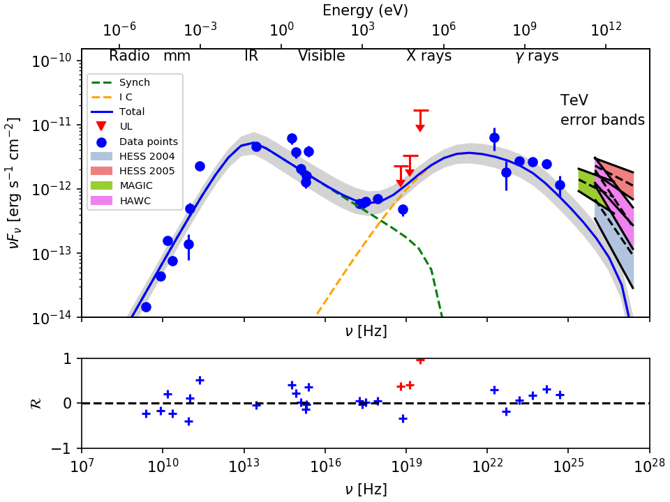
Figure 1: SED of M87 with the best fit SSC model. Blue points correspond to measured fluxes taken from Morabito et al. (1986), Morabito et al. (1988), Junor & Biretta (1995), Lee et al. (2008), Lonsdale, Colin J and Doeleman, Sheperd S and Phillips, Robert B (1998), Doeleman et al. (2012), Biretta et al. (1991), Perlman et al. (2001), Sparks et al. (1996), Marshall et al. (2002), Wong et al. (2017), Abdo et al. (2009) and the 4FGL catalog Abdollahi et al. (2020). The model of the synchrotron component is the orange dashed curve and the model of the inverse Compton component is the green dashed curve. Swift/BAT upper limits obtained by Abdo et al. (2009) are shown by red triangles. The gray region corresponds to the 1 $\sigma$ error of the best fit model parameters. For comparison, TeV error bands from 2004 H.E.S.S (blue) (Aharonian et al., 2006), 2005 H.E.S.S (red) (Aharonian et al., 2006), MAGIC (green) (Aleksić et al., 2012) and HAWC (violet) (Albert et al., 2021) are shown. Residuals of the best fit model, which are defined as $\mathcal{R}=\log(F_{\nu,obs}/F_{\nu,mod})$ where $F_{\nu,obs}$ and $F_{\nu,mod}$ are the observed and predicted flux respectively, are shown in the bottom panel.

As mentioned before, we considered four different VHE data sets for modeling the VHE emission of M87. The best fit values for the photo-hadronic model parameters are presented in Table 2. The best fit models, data and residuals are plotted in Figure 2.

Table 2: Best fit values for the photo-hadronic component fitting parameters with their error estimates

	$\alpha$	$A_{\gamma}$	$\chi_{\nu}^{2}$(d.o.f)
H.E.S.S. : 2004 observations a	$3.2^{+0.2}_{-0.4}$	$0.1^{+0.2}_{-0.1}$	25.5 (22)
H.E.S.S.: 2005 observations a	$2.8\pm 0.2$	$0.6^{+0.4}_{-0.2}$	22.5 (22)
MAGIC: 2005-2007 observations b	$3.0\pm 0.2$	$0.2^{+0.2}_{-0.1}$	23.7 (26)
HAWC observations (1523 days) c	$3.1\pm 0.2$	$0.2\pm 0.1$	25.8 (22)

Note. — $\alpha$ Proton energy distribution index, $A_{\gamma}$ normalization constant

^a Data taken from Aharonian et al. (2006)

^b Data taken from Aleksić et al. (2012)

$c$ Data taken from Albert et al. (2021).

Figure 2: SED of M87 with the photo-hadronic model fit for data from 2004 H.E.S.S. data (Aharonian et al., 2006) (a), 2005 H.E.S.S. data (Aharonian et al., 2006) (b), 2005-2007 MAGIC data (Aleksić et al., 2012)(c) and 2014-2019 HAWC (Albert et al., 2021)(d). The SSC model is identical to that of Figure 1. Measured fluxes are plotted in blue. The synchrotron component is the orange dashed curve and the inverse Compton component is the green dashed curve. Swift/BAT upper limits are shown with red triangles. The model of the photo-hadronic component is the red dashed curve. Residuals of the models, which are defined as $\mathcal{R}=\log(F_{\nu,obs}/F_{\nu,mod})$ where $F_{\nu,obs}$ and $F_{\nu,mod}$ are the observed and predicted flux respectively, are shown below each plot.

6 Discussion

We constructed a broadband SED using data from steady state epochs. It was fit with a lepto-hadronic model in order to explain its VHE emission. The lepto-hadronic model is a combination of the one-zone SSC model proposed by Finke et al. (2008) and the photo-hadronic model used by Sahu (2019). The model proposes the existence of three components: a synchrotron dominated component from radio to X-rays, an inverse Compton dominated component from X-rays to GeV gamma rays and a photo-hadronic dominated component in the range of TeV gamma rays.

As shown in Figure 1, the SSC model provides a good fit to the SED up to GeV gamma rays, but it underestimates the VHE emission, consistently with what is found in the literature (e.g. Fraija & Marinelli, 2016; Ait Benkhali et al., 2019). The X-ray emission was of particular interest for corresponding to the transition between both components of the SSC scenario. X rays are also important to produce the VHE emission in the photo-hadronic scenario, because the typical energies of the target photons for the photo-hadronic interactions fall in the X-ray range. The only X-ray data point which could not be well fit was the NuSTAR 20-40 KeV observation. In Wong et al. (2017), which reported this observation, they also discussed its inconsistency with inverse Compton models to explain gamma ray emission. According to them, the observation uncertainties are limited by the statistical power of their data and deeper observations are necessary to resolve the tension with the NuSTAR data.

Table 3 shows a comparison of the SSC parameters values obtained by different studies. Two of them (the magnetic field intensity and the break Lorentz factor) present a dispersion of several orders of magnitude. This dispersion can be caused by degeneracy in the SED models, different assumptions in the emission zone geometry or different level of completeness in the data sets. In the case of magnetic field intensity ($B$), most of the degeneracy comes from the relation $B\delta^{2}R_{b}^{\prime}\approx$ constant (Finke et al., 2008), which was first derived by Tavecchio et al. (1998). As this relation holds in every case of Table 3 ($B\delta^{2}R_{b}^{\prime}\approx(2-4)\times 10^{16}$), variations in the magnetic field intensity ($B$) can be caused by different assumptions regarding the radius of the emission zone $R_{b}^{\prime}$. The other parameters have less dispersion. It is important to remark that the lack of error estimates for most of the parameters reported in the literature prevents a more precise comparison of these results.

Parameter	This study	Abdo et al. (2009)	De Jong et al. (2015)	Fraija & Marinelli (2016)	Acciari et al. (2020)
$B$(G)	$0.046\pm 0.003$	$0.055$	$0.002$	$1.61$	$0.0031$
$\delta$	$4.3\pm 0.2$	$3.9$	$5$	$2.8$	$5.3$
$p_{1}$	$1.52\pm 0.02$	$1.6$	$-1.8$	$3.21\pm 0.02$	$1.9$
$p_{2}$	$3.53\pm 0.02$	$3.6$	$3.4$	$4.21$	$3.2$
$\gamma_{c}^{\prime}$	$3.80^{+0.06}_{-0.05}\times 10^{3}$	$4\times 10^{3}$	$4.0\times 10^{2}$	$1.7\times 10^{3}$	$1.4\times 10^{4}$
$R_{b}^{\prime}$(cm)	$(1.54\pm 0.07)\times 10^{16}$	$1.4\times 10^{16}$	$5.6\times 10^{17}$	$2.1\times 10^{15}$	$4.0\times 10^{17}$

Table 3: Comparison of results for the SSC parameters from different studies. All the SEDs were constructed to model the non-flaring state of M87

The viewing angle ($\theta$) plays an important role in AGN properties. According to unification schemes, the transition between blazars and RDGs is produced around $\theta\sim 10^{\circ}$. The Doppler factor can be constrained from $\theta$ by (Abdo et al., 2010):

$$\delta\leq\frac{1}{\sin(\theta)}.$$ (10)

Higher Doppler factors enhance the HE and VHE emission, which explains why many more blazars have been detected at gamma ray energies than RDGs.

The Doppler factor value obtained in this work ($\delta=4.3\pm 0.2$) is consistent with the lowest estimates for the viewing angle ($\theta\approx 10^{\circ}-20^{\circ}$) (Biretta et al., 1999), which have been based mainly on optical observations of the jet feature HST-1. However, it is in disagreement with other estimates ($\theta\approx 30^{\circ}-45^{\circ}$) (Ly et al., 2007) based on VLBI observations of the jet base of M87. In fact, all the values for $\delta$ presented in Table 3 are inconsistent with the VLBI measurements. One way to solve this tension is taking into account the width of the jet base. According to Hada et al. (2016) the M87 jet base has an apparent opening angle of $\sim 100^{\circ}$, which would correspond to an intrinsic opening angle of $\sim 50^{\circ}$ (if $\theta\sim 30^{\circ}$). Therefore, a VHE emission zone located in the outer zones of the jet base could have a viewing angle as low as $\sim 5^{\circ}$, which would be consistent with a Doppler factor $\delta\leq 11.8$.

As shown in Figure 2, the photo-hadronic component is able to explain the VHE emission in both flaring and quiescent states. This component is produced by the interaction between inverse Compton photons and accelerated protons from the jet. We studied the quiescent state using three different sets of TeV data: H.E.S.S. observations from 2004, MAGIC observations from 2005-2007 and HAWC observations from the 2014-2019 period (all three of them without VHE flares). The high activity state was studied using H.E.S.S. data corresponding to the 2005 VHE flare. There were no reports of inner jet high activity in other bands during that flare. That is why we used the same broadband SED as in the non-flaring state. HAWC results were in agreement with the 2004 H.E.S.S. observations and the MAGIC observations, but HAWC fluxes are lower than the fluxes of the 2005 flaring state. This indicates that HAWC observations constrain the average VHE emission from M87 during quiescent periods.

The proton energy distribution index $\alpha$ was estimated with the four VHE data sets . Those measurements agree with the result obtained by Fraija & Marinelli (2016) $\alpha=2.80\pm 0.02$ where a similar lepto-hadronic model was used to fit the 2004 H.E.S.S. data. It is also important to remark the change in $\alpha$ observed in the 2005 H.E.S.S. observation with respect to other TeV results and the lack of high activity in the other bands during this flare. Those results indicate that the flare could have been caused by an energy increase of the accelerated proton population.

It is important to mention that HAWC data are the only continuous TeV measurements. The IACT observations are made with exposure times corresponding to a few hours that could be affected by rapid VHE flux variations. Therefore, HAWC results represent a steadier constraint to the mean VHE emission of M87 during the HAWC’s period of observation.

With these results, we calculated an electron luminosity of $L_{e}\sim 7\times 10^{42}$ erg/s. Accelerated proton flux ($F_{p}$) and luminosity ($L_{p}$) can also be estimated using Equation below (Sahu, 2019),

$$F_{p}(E_{p})\approx 10\times\frac{f^{p\gamma}(\epsilon_{\Gamma})}{\tau_{p\gamma}(E_{p})},$$ (11)

where $f^{p\gamma}(\epsilon_{\Gamma})$ is given by Equation 8 and $\tau_{p\gamma}$ is the optical depth of the $\Delta$ resonance process in the inner jet region. As mentioned before, this model assumes the photo-hadronic interactions to occur in an inner compact region of the blob with a smaller size and a higher photon density. Unfortunately, these quantities are not directly observable and the value of $\tau_{p\gamma}$ cannot be calculated. However, Sahu (2019) gives two prescriptions $\tau_{p\gamma}<$ 2 and $\tau_{p\gamma}>f^{p\gamma}(\epsilon_{\Gamma})/f_{Edd}$, where $f_{Edd}$ is the Eddington flux. As in this case $f^{p\gamma}(\epsilon_{\Gamma})/f_{Edd}\approx 10^{-7}$, we assumed the intermediate value $\tau_{p\gamma}\approx 10^{-2}$ and we obtained a proton luminosity of $L_{p}\sim 6\times 10^{43}$ erg/s. These results are in agreement with the total jet power estimates $L_{j}\sim 10^{44}$ erg/s (Owen et al., 2000).

The decay of charged pions produces neutrinos. The neutrino flux ($f^{\nu}$) can be estimated assuming (Aartsen et al., 2020):

$$E_{\nu}\approx\epsilon_{\Gamma}/2,$$ (12)

where $E_{\nu}$ is the emitted neutrino energy, and also (Murase et al., 2016):

$$f^{\nu}(E_{\nu})\approx\frac{3}{4}f^{p\gamma}(\epsilon_{\Gamma}/2).$$ (13)

The estimated neutrino flux for $E_{\nu}=5$ TeV corresponds to $\epsilon_{\Gamma}=10$ TeV, is $f^{\nu}\sim 1\times 10^{-13}$ TeV cm^-2 s^-1, which is below IceCube upper limits (Aartsen et al., 2020).

As with regard to the results of some other alternative models, in Fraija & Marinelli (2016) the SED of M87 was fit with a very similar lepto-hadronic model. In this case, VHE emission was represented only by the 2004 H.E.S.S. results, which were obtained with just $\sim 50$ hours of observation. However, the best fitting values of the photo-hadronic parameters were in agreement, within their uncertainties, with those obtained in this work. In Sahu & Palacios (2015) a lepto-hadronic scenario was used to explain the 2010 TeV flare and their results were also in agreement with those obtained in this work. However, this flare had an X-ray counterpart (Abramowski et al., 2012), which may be interpreted as purely leptonic. A leptonic and a hybrid model were used to model MAGIC results from a 2012-2015 campaign (Acciari et al., 2020), where they found the hybrid model was more consistent with gamma ray data. Finally, according to Ait Benkhali et al. (2019), extended gamma ray production scenarios such as Compton scattering in the kiloparsec-scale jet (e.g., Hardcastle & Croston, 2011) are disfavored by gamma ray variability.

We cannot rule a purely leptonic scenario out. Actually, multi-zone structured leptonic models are necessary to explain specific features in the whole MWL SED (Algaba et al., 2021). However, these models have a large number of parameters, which introduces a high degeneracy, making it difficult to derive firm conclusions from their fit. As the aim of this paper is explaining the VHE emission, we decided to use a one-zone SSC scenario to model the leptonic contribution

7 Conclusions

M87 is considered a laboratory for understanding AGN properties since it is the only source that has been mapped from the SMBH shadow ($\sim 0.005$ pc) to the outer jet ($\sim 25$ kpc). Understanding its gamma ray emission, which is practically unaffected by EBL absorption up to $\sim$ 10 TeV, could be the key to understanding gamma ray emission in the rest of the AGNs (not only RDGs). We fit a broadband SED of M87 with a lepto-hadronic model with the aim of explaining its VHE emission. Emission from radio to GeV gamma rays has been modeled with an SSC scenario. The best fit values for SSC model parameters were for the Doppler factor $\delta=$ $4.3\pm 0.2$, for the mean magnetic field intensity $B=$ $0.046\pm 0.003$ G, for the electron energy distribution parameters $p_{1}=$ $1.52\pm 0.02$, $p_{2}=$ $3.53\pm 0.02$ and $\gamma_{c}^{\prime}=$ $3.80^{+0.6}_{-0.5}\times 10^{3}$. The value of the Doppler factor is in agreement with a low viewing angle of the jet base ($\theta\sim 13^{\circ}$). However, a large viewing angle is also possible if the opening angle of the jet base is wide enough to place the emission zone closer to the observer’s line of sight.

A photo-hadronic model was fit to the VHE emission. Results show that this model is able to explain the quiescent VHE emission represented by H.E.S.S., MAGIC and HAWC observations. H.E.S.S. data corresponding to the 2005 VHE flare were also fit using this model. The results show that the model can explain the so called orphan flares, which are only detected at VHE bands, such as the one observed in 2005. Those flares would be produced by changes in the proton energy distribution.

HAWC observations constrained the VHE emission from M87 for the 2014-2019 period in which no evidence of VHE flares was reported. We obtained a proton energy distribution power law index of $\alpha=3.1\pm 0.2$ and TeV gamma ray flux normalization constant of $A_{\gamma}=0.2\pm 0.1$. HAWC will be taking data for a few more years. Therefore, the significance of the M87 detection will probably be improved allowing a better estimation of the photo-hadronic model parameters.

8 ACKNOWLEDGMENTS

We acknowledge the support from: the US National Science Foundation (NSF); the US Department of Energy Office of High-Energy Physics; the Laboratory Directed Research and Development (LDRD) program of Los Alamos National Laboratory; Consejo Nacional de Ciencia y Tecnología (CONACyT), México, grants 271051, 232656, 260378, 179588, 254964, 258865, 243290, 132197, A1-S-46288, A1-S-22784, cátedras 873, 1563, 341, 323, Red HAWC, México; DGAPA-UNAM grants IG101320, IN111716-3, IN111419, IA102019, IN110621, IN110521; VIEP-BUAP; PIFI 2012, 2013, PROFOCIE 2014, 2015; the University of Wisconsin Alumni Research Foundation; the Institute of Geophysics, Planetary Physics, and Signatures at Los Alamos National Laboratory; Polish Science Centre grant, DEC-2017/27/B/ST9/02272; Coordinación de la Investigación Científica de la Universidad Michoacana; Royal Society - Newton Advanced Fellowship 180385; Generalitat Valenciana, grant CIDEGENT/2018/034; Chulalongkorn University’s CUniverse (CUAASC) grant; Coordinación General Académica e Innovación (CGAI-UdeG), PRODEP-SEP UDG-CA-499; Institute of Cosmic Ray Research (ICRR), University of Tokyo, H.F. acknowledges support by NASA under award number 80GSFC21M0002. We also acknowledge the significant contributions over many years of Stefan Westerhoff, Gaurang Yodh and Arnulfo Zepeda Dominguez, all deceased members of the HAWC collaboration. Thanks to Scott Delay, Luciano Díaz and Eduardo Murrieta for technical support.

References

- Aartsen et al. (2018) Aartsen, M., Ackermann, M., Adams, J., et al. 2018, Science, 361, 147
- Aartsen et al. (2020) Aartsen, M. G., Ackermann, M., Adams, J., et al. 2020, Phys. Rev. Lett., 124, 051103, doi: 10.1103/PhysRevLett.124.051103
- Abdo et al. (2009) Abdo, A., Ackermann, M., Ajello, M., et al. 2009, The Astrophysical Journal, 707, 55
- Abdo et al. (2010) —. 2010, The Astrophysical Journal, 719, 1433
- Abdollahi et al. (2020) Abdollahi, S., Acero, F., Ackermann, M., et al. 2020, The Astrophysical Journal Supplement Series, 247, 33, doi: 10.3847/1538-4365/ab6bcb
- Abeysekara et al. (2017) Abeysekara, A., Albert, A., Alfaro, R., et al. 2017, The Astrophysical Journal, 843, 39
- Abramowski et al. (2012) Abramowski, A., Acero, F., Aharonian, F., et al. 2012, The Astrophysical Journal, 746, 151
- Acciari et al. (2010) Acciari, V., Aliu, E., Arlen, T., et al. 2010, The Astrophysical Journal, 716, 819
- Acciari et al. (2020) Acciari, V., Ansoldi, S., Antonelli, L., et al. 2020, Monthly Notices of the Royal Astronomical Society
- Aharonian et al. (2003) Aharonian, F., Akhperjanian, A., Beilicke, M., et al. 2003, Astronomy & Astrophysics, 403, L1
- Aharonian et al. (2006) Aharonian, F., Akhperjanian, A. G., Bazer-Bachi, A. R., et al. 2006, Science, 314, 1424, doi: 10.1126/science.1134408
- Ait Benkhali et al. (2019) Ait Benkhali, F., Chakraborty, N., & Rieger, F. M. 2019, Astronomy & Astrophysics, 623, A2
- Albert et al. (2021) Albert, A., Alvarez, C., Camacho, J. R. A., et al. 2021, The Astrophysical Journal, 907, 67, doi: 10.3847/1538-4357/abca9a
- Albert et al. (2008) Albert, J., Aliu, E., Anderhub, H., et al. 2008, The Astrophysical Journal Letters, 685, L23
- Aleksić et al. (2012) Aleksić, J., Alvarez, E., Antonelli, L., et al. 2012, Astronomy & Astrophysics, 544, A96
- Algaba et al. (2021) Algaba, J., Anczarski, J., Asada, K., et al. 2021, The Astrophysical journal letters, 911, L11
- Astropy Collaboration et al. (2018) Astropy Collaboration, Price-Whelan, A. M., Sipőcz, B. M., et al. 2018, AJ, 156, 123, doi: 10.3847/1538-3881/aabc4f
- Bird et al. (2010) Bird, S., Harris, W. E., Blakeslee, J. P., & Flynn, C. 2010, Astronomy & Astrophysics, 524, A71
- Biretta et al. (1999) Biretta, J., Sparks, W., & Macchetto, F. 1999, The Astrophysical Journal, 520, 621
- Biretta et al. (1991) Biretta, J., Stern, C., & Harris, D. 1991, The Astronomical Journal, 101, 1632
- Blandford et al. (2019) Blandford, R., Meier, D., & Readhead, A. 2019, Annual Review of Astronomy and Astrophysics, 57, 467
- Cheung et al. (2007) Cheung, C., Harris, D., et al. 2007, The Astrophysical Journal Letters, 663, L65
- Curtis (1918) Curtis, H. D. 1918, Publications of Lick Observatory, 13, 9
- De Jong et al. (2015) De Jong, S., Beckmann, V., Soldi, S., Tramacere, A., & Gros, A. 2015, Monthly Notices of the Royal Astronomical Society, 450, 4333
- Dermer & Menon (2009) Dermer, C. D., & Menon, G. 2009, High energy radiation from black holes: gamma rays, cosmic rays, and neutrinos, Vol. 17 (Princeton University Press)
- Doeleman et al. (2012) Doeleman, S. S., Fish, V. L., Schenck, D. E., et al. 2012, Science, 338, 355
- Doherty et al. (2009) Doherty, M., Arnaboldi, M., Das, P., et al. 2009, Astronomy & Astrophysics, 502, 771
- Domínguez et al. (2011) Domínguez, A., Primack, J. R., Rosario, D., et al. 2011, Monthly Notices of the Royal Astronomical Society, 410, 2556
- Finke et al. (2008) Finke, J. D., Dermer, C. D., & Böttcher, M. 2008, The Astrophysical Journal, 686, 181
- Fraija & Marinelli (2016) Fraija, N., & Marinelli, A. 2016, The Astrophysical Journal, 830, 81
- Georganopoulos et al. (2005) Georganopoulos, M., Perlman, E. S., & Kazanas, D. 2005, The Astrophysical Journal Letters, 634, L33
- Hada et al. (2016) Hada, K., Kino, M., Doi, A., et al. 2016, The Astrophysical Journal, 817, 131
- Hardcastle & Croston (2011) Hardcastle, M., & Croston, J. 2011, Monthly Notices of the Royal Astronomical Society, 415, 133
- Harris et al. (2020) Harris, C. R., Millman, K. J., van der Walt, S. J., et al. 2020, Nature, 585, 357, doi: 10.1038/s41586-020-2649-2
- Harris et al. (2006) Harris, D., Cheung, C., Biretta, J., et al. 2006, The Astrophysical Journal, 640, 211
- Hunter (2007) Hunter, J. D. 2007, Computing in Science & Engineering, 9, 90, doi: 10.1109/MCSE.2007.55
- Junor & Biretta (1995) Junor, W., & Biretta, J. A. 1995, The Astronomical Journal, 109, 500
- Lee et al. (2008) Lee, S.-S., Lobanov, A. P., Krichbaum, T. P., et al. 2008, The Astronomical Journal, 136, 159
- Longair (2011) Longair, M. S. 2011, High energy astrophysics (Cambridge University Press)
- Lonsdale, Colin J and Doeleman, Sheperd S and Phillips, Robert B (1998) Lonsdale, Colin J and Doeleman, Sheperd S and Phillips, Robert B. 1998, The Astronomical Journal, 116, 8
- Ly et al. (2007) Ly, C., Walker, R. C., & Junor, W. 2007, The Astrophysical Journal, 660, 200
- Marshall et al. (2002) Marshall, H. L., Miller, B., Davis, D., et al. 2002, The Astrophysical Journal, 564, 683
- Morabito et al. (1986) Morabito, D., Niell, A., Preston, R., et al. 1986, The Astronomical Journal, 91, 1038
- Morabito et al. (1988) Morabito, D. D., Preston, R. A., & Jauncey, D. L. 1988, The Astronomical Journal, 95, 1037
- Mücke et al. (2003) Mücke, A., Protheroe, R., Engel, R., Rachen, J., & Stanev, T. 2003, Astroparticle Physics, 18, 593
- Murase et al. (2016) Murase, K., Guetta, D., & Ahlers, M. 2016, Phys. Rev. Lett., 116, 071101, doi: 10.1103/PhysRevLett.116.071101
- Owen et al. (2000) Owen, F. N., Eilek, J. A., & Kassim, N. E. 2000, The Astrophysical Journal, 543, 611
- Perlman et al. (1999) Perlman, E. S., Biretta, J. A., Zhou, F., Sparks, W. B., & Macchetto, F. D. 1999, The Astronomical Journal, 117, 2185
- Perlman et al. (2001) Perlman, E. S., Sparks, W. B., Radomski, J., et al. 2001, The Astrophysical Journal Letters, 561, L51
- Press et al. (2007) Press, W. H., Teukolsky, S. A., Vetterling, W. T., & Flannery, B. P. 2007, Numerical recipes 3rd edition: The art of scientific computing (Cambridge University Press)
- Prieto et al. (2016) Prieto, M., Fernández-Ontiveros, J., Markoff, S., Espada, D., & González-Martín, O. 2016, Monthly Notices of the Royal Astronomical Society, 457, 3801
- Reynoso et al. (2011) Reynoso, M., Medina, M., & Romero, G. 2011, Astronomy & Astrophysics, 531, A30
- Rieger & Levinson (2018) Rieger, F. M., & Levinson, A. 2018, Galaxies, 6, 116
- Rybicki & Lightman (2008) Rybicki, G. B., & Lightman, A. P. 2008, Radiative processes in astrophysics (John Wiley & Sons)
- Sahu (2019) Sahu, S. 2019, Revista mexicana de física, 65, 307
- Sahu et al. (2019) Sahu, S., Fortín, C. E. L., & Nagataki, S. 2019, The Astrophysical Journal Letters, 884, L17
- Sahu & Palacios (2015) Sahu, S., & Palacios, E. 2015, The European Physical Journal C, 75, 1
- Sparks et al. (1996) Sparks, W., Biretta, J., & Macchetto, F. 1996, The Astrophysical Journal, 473, 254
- Tavecchio et al. (1998) Tavecchio, F., Maraschi, L., & Ghisellini, G. 1998, The Astrophysical Journal, 509, 608
- The EHT Collaboration et al. (2019) The EHT Collaboration, et al. 2019, The Astrophysical Journal Letters, 875, 1. https://iopscience.iop.org/article/10.3847/2041-8213/ab0ec7
- Ureña-Mena et al. (2021) Ureña-Mena, F., Carramiñana, A., Longinotti, A. L., Rosa-González, D., & the HAWC Collaboration. 2021, PoS(ICRC2021), 395, 841. https://pos.sissa.it/395/841/pdf
- Urry & Padovani (1995) Urry, C. M., & Padovani, P. 1995, Publications of the Astronomical Society of the Pacific, 107, 803
- Van Rossum & Drake Jr (1995) Van Rossum, G., & Drake Jr, F. L. 1995, Python reference manual (Centrum voor Wiskunde en Informatica Amsterdam)
- Wong et al. (2017) Wong, K.-W., Nemmen, R. S., Irwin, J. A., & Lin, D. 2017, The Astrophysical Journal Letters, 849, L17
- Yamada et al. (2020) Yamada, Y., Uemura, M., Itoh, R., et al. 2020, arXiv preprint arXiv:2003.08016
- Zhu et al. (2014) Zhu, L., Long, R., Mao, S., et al. 2014, The Astrophysical Journal, 792, 59