An Empirical Investigation of the Role of Pre-training in Lifelong Learning

Abstract

The lifelong learning paradigm in machine learning is an attractive alternative to the more prominent isolated learning scheme not only due to its resemblance to biological learning but also its potential to reduce energy waste by obviating excessive model re-training. A key challenge to this paradigm is the phenomenon of catastrophic forgetting. With the increasing popularity and success of pre-trained models in machine learning, we pose the question: What role does pre-training play in lifelong learning, specifically with respect to catastrophic forgetting? We investigate existing methods in the context of large, pre-trained models and evaluate their performance on a variety of text and image classification tasks, including a large-scale study using a novel data set of 15 diverse NLP tasks. Across all settings, we observe that generic pre-training implicitly alleviates the effects of catastrophic forgetting when learning multiple tasks sequentially compared to randomly initialized models. We then further investigate why pre-training alleviates forgetting in this setting. We study this phenomenon by analyzing the loss landscape, finding that pre-trained weights appear to ease forgetting by leading to wider minima. Based on this insight, we propose jointly optimizing for current task loss and loss basin sharpness to explicitly encourage wider basins during sequential fine-tuning. We show that this optimization approach outperforms several state-of-the-art task-sequential continual learning algorithms across multiple settings, occasionally even without retaining a memory that scales in size with the number of tasks.

Keywords: Lifelong Learning, Continual Learning, Pre-training, Flat Minima, Sharpness-Aware Minimization

1 Introduction

The contemporary machine learning paradigm concentrates on isolated learning (Chen and Liu, 2018) i.e., learning a model from scratch for every new task. In contrast, the lifelong learning (Thrun and Mitchell, 1995; Thrun, 1996; Chen and Liu, 2018) or incremental learning (Solomonoff et al., 1989; Syed et al., 1999; Ruping, 2001) or never-ending learning (Mitchell et al., 2018) or continual learning (Parisi et al., 2019) paradigm defines a biologically-inspired learning approach where models learn tasks in sequence, ideally preserving past knowledge and leveraging it to efficiently learn new tasks. Lifelong learning has the added benefit of avoiding periodical re-training of models from scratch to learn novel tasks or adapt to new data, with the potential to reduce both computational and energy requirements (Hazelwood et al., 2018; Strubell et al., 2019; Schwartz et al., 2020). In the context of modern machine learning where state-of-the-art models are powered by deep neural networks, catastrophic forgetting has been identified as a key challenge to implementing successful lifelong learning systems (McCloskey and Cohen, 1989; French, 1999). Catastrophic forgetting happens when the model forgets knowledge learned in previous tasks as information relevant to the current task is incorporated. Mitigating or preventing this phenomenon is critical to achieving true lifelong learning.

At the same time, transfer learning has shown impressive results in both computer vision (CV; Zhuang et al. 2021) and natural language processing (NLP) applications (Howard and Ruder, 2018; Peters et al., 2018; Devlin et al., 2019). The modern transfer learning paradigm involves pre-training a fixed architecture, like ResNet (He et al., 2016) or BERT (Devlin et al., 2019), using copious amounts of data, and then fine-tuning the learnt parameters on target tasks. Given the tremendous success of pre-trained models, there has been increased interest in understanding their role in improving generalization (Erhan et al., 2010; Neyshabur et al., 2020), speed of convergence (Hao et al., 2019), successful transfer (He et al., 2019; Pruksachatkun et al., 2020), and out-of-distribution robustness (Hendrycks et al., 2020; Tu et al., 2020). Despite these efforts, the role of pre-trained initializations in lifelong learning settings has been under-explored. In contemporary work, it has been shown that pre-trained models can be used as feature extractors (i.e., pre-trained weights are frozen) for task-sequential learning (Hu et al., 2021). Because the pre-trained weights are explicitly frozen in this setting, the model undergoes no catastrophic forgetting. In contrast, fine-tuning pre-trained weights update the pre-trained model parameters and are susceptible to severe forgetting. This is typically the most accurate and thus common transfer learning paradigm (Peters et al., 2019), and the one we consider in this work. To the best of our knowledge, there is no prior work systematically analyzing the role of pre-trained initialization on catastrophic forgetting in lifelong learning scenarios.

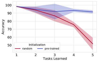
Figure 1: Pre-trained and randomly initialized DistilBERT on Split YahooQA data set. Performance of the first task visualized over sequential learning of tasks (averaged over $5$ runs). Both models start with approximately equal average task accuracy, but pre-trained initialization leads to significantly less forgetting.

Figure 1 shows that simply changing the network initialization to generic pre-trained weights can significantly reduce forgetting on the first task when doing sequential training on five tasks. This observation motivates us to ask—Does pre-training implicitly alleviate catastrophic forgetting, and if so, why? To answer this question we conduct a systematic study on existing CV and NLP benchmarks and observe that pre-training indeed leads to less forgetting. We also investigate the effect of the type of pre-trained initialization by analyzing the extent to which different pre-trained Transformer language model variants (Sanh et al., 2019; Devlin et al., 2019; Liu et al., 2019) undergo forgetting, observing that increasing the capacity of the model and diversity of the pre-training corpus play an important role in alleviating forgetting. To further stress-test these models under realistic scenarios, we introduce a data set with 15 diverse NLP tasks and observe a considerable increase in forgetting on this data set.

We hypothesize that pre-trained weights already have a good inductive bias to implicitly alleviate forgetting. To explain this behavior, we build upon two separate observations—Hao et al. (2019); Neyshabur et al. (2020) show that in the context of transfer learning, pre-trained weights lead to a flat loss basin when fine-tuning on a single task. Mirzadeh et al. (2020) argues that the geometric properties of the local minima for each task play a vital role in forgetting, and they suggest modifying the hyper-parameters (learning rate decay, batch size, dropout) to promote flat minima.

To verify the above hypothesis, we analyze the loss landscape of the first task as the model is trained sequentially on subsequent tasks. For pre-trained initializations, we see that minima obtained after training on a sequence of tasks still remain in the relatively low loss basin of the first task when compared with random initialization. Further, linearly interpolating loss across sequentially trained task minima confirms that models initialized with pre-trained weights undergo a more gradual change in loss compared to random initialization. These observations hint at the flatness of the minima reached in the case of pre-trained initialized models. To quantify the flatness of the loss landscape, we compute a sharpness metric (Keskar et al., 2017) and verify that pre-trained weights indeed lead to flat basins in comparison to random weights while training sequentially. These analyses help us showcase that continual training from pre-trained weights induces wide task minima, therefore, implicitly alleviating forgetting. To further mitigate forgetting, we explicitly optimize for flat loss basins by minimizing the current task loss and the sharpness metric. Concretely, we use the Sharpness-Aware Minimization (SAM) procedure (Foret et al., 2021) to seek parameters that lie in the neighborhoods having uniformly low loss values (Section 5) and report improved results across many experimental settings. Our main contributions can be summarized as follows:

• We observe that initializing models with pre-trained weights results in less forgetting compared to random weights despite achieving higher performance on each task. We bolster this observation with a systematic study validating that this behavior persists across applications (NLP, CV) and prominent approaches: Elastic weight consolidation (Kirkpatrick et al., 2017), A-GEM (Chaudhry et al., 2018b), and episodic replay (Chaudhry et al., 2019) (Section 3.1).

• To understand the role of varying pre-trained initializations, we analyze a suite of pre-trained Transformer language models and showcase that model capacity and diversity of the pre-training corpus do play a role in alleviating forgetting. We also show that sequential training on diverse tasks is still challenging for pre-trained initialized models by introducing a new, more challenging benchmark for lifelong learning in NLP consisting of 15 diverse NLP tasks (Sections 3.2,3.3).

• We hypothesize and verify empirically that pre-trained models alleviate forgetting as they have an implicit bias towards wider task minima. The effect of these wider minima is that changes in weights from learning subsequent tasks result in a smaller change to the current task loss, which helps reduce forgetting (Section 4).

• We further show that explicitly seeking flat minima during task incremental learning leads to reduced forgetting and achieves state-of-the-art performance on the benchmarks we considered. Our analysis of different initializations, namely task-agnostic meta-learned and supervised pre-trained models explicitly guided towards flat loss regions, highlights the synergistic benefits when combined with the explicit optimization for flatness during sequential fine-tuning (Section 5).

2 Preliminaries

In this section, we introduce the notations and outline our problem setup. We also specify our experimental settings, including the baseline methods, benchmarks, and evaluation metrics.

2.1 Problem Setup: Task Incremental Learning

We consider a setup where we receive a continuum of data from different tasks sequentially: $(x_{1},y_{1},t_{1}),\cdots,(x_{i},y_{i},t_{i}),\cdots$. Each triplet $(x_{i},y_{i},t_{i})$ consists of a task descriptor $t_{i}\in\mathcal{T}$, input data $x_{i}\in\mathcal{D}_{t_{i}}$, target labels $y_{i}\in\mathcal{Y}_{t_{i}}$ and satisfies $(x_{i},y_{i})\stackrel{{\scriptstyle iid}}{{\sim}}\mathcal{P}_{t_{i}}(X,Y)$. Following (Chaudhry et al., 2019), we consider an explicit task descriptor $t_{i}$ because the same input $x_{i}$ can appear in multiple different tasks but with different labels. For example, given a product review, we could annotate it with sentiment polarity and grammatical acceptability judgments. Given the observed data, our goal is to learn a predictor $f:\mathcal{X}\times\mathcal{T}\rightarrow\mathcal{Y}$ where we want to evaluate test pairs $(x,t)$ from previously observed tasks (backward transfer) and the current task at any time during task incremental learning of our model (Van de Ven and Tolias, 2019).

2.2 Benchmarks

We perform extensive experiments on widely adopted task-incremental learning benchmarks (Chaudhry et al., 2019; Ebrahimi et al., 2020; Wang et al., 2020) across both CV and NLP domains. These benchmarks help us evaluate our method to be consistent with the literature. Most of the existing works consider Split MNIST, Split CIFAR-10, and Split CIFAR-100 benchmarks, which are homogenous; different tasks in these benchmarks share the same underlying domain. Given the generic nature of the pre-trained initialization, we want to investigate forgetting when subjected to a sequence of diverse tasks. Therefore, we also consider data sets spanning diverse CV and NLP tasks.

Data set	|Train|	|Dev|	|Test|	|L|
MNIST	51,000	9,000	10,000	10
notMNIST	15,526	2,739	459	10
Fashion-MNIST	9,574	1,689	1,874	10
CIFAR10	42,500	7,500	10,000	10
SVHN	62,269	10,988	26,032	10

Table 1: 5-dataset-CV statistics. |Train|, |Dev|, |Test| denotes the number of examples in the train, dev, and test splits respectively. |L| denotes the number of classes for each task.

2.2.1 CV Benchmarks

Below, we provide further details on the data sets we utilized for our CV experiments: 5-dataset-CV (diverse) and Split CIFAR-50/ Split CIFAR-100 (homogenous).

• 5-dataset-CV consists of five diverse 10-way image classification tasks: CIFAR-10 (Krizhevsky and Hinton, 2009), MNIST (LeCun, 1998), Fashion-MNIST (Xiao et al., 2017), SVHN (Netzer et al., 2011), and notMNIST (Bulatov, 2011). It is one of the largest data sets used for lifelong learning experiments (Ebrahimi et al., 2020) with overall $180.9$k train examples (see Table 1 for task-specific statistics).

• Split CIFAR-50 takes the first 50 classes of the CIFAR-100 image classification data set (Krizhevsky and Hinton, 2009) and randomly splits them into five homogenous 10-way classification tasks. Each task contains $5,000/1,000$ (train/test) examples. We built this data set as a homogenous counterpart to 5-dataset-CV by mimicking its task structure (10 classes/task) and the number of tasks. Further, we note that Split CIFAR-50 (10 classes/ task) is more challenging than Split MNIST/ CIFAR-10 (2 classes/ task) because of the more number of classes per task. Therefore, in this work, we prefer Split CIFAR-50 over MNIST/CIFAR-10 for our experimentation.

• Split CIFAR-100 splits the CIFAR-100 data set into 20 disjoint 5-way classification tasks, with each task containing $2,500/500$ (train/test) examples. Due to the large number of tasks in this data set, it is regarded as one of the most challenging and realistic CV benchmarks for lifelong learning (Chaudhry et al., 2018b).

Task	Data set/	Domain(s)/	|Train|	|Dev|	|Test|	|L|	Metrics
	Corpus	Text source(s)
Linguistic	CoLA	Journal articles	7,695	856	1,043	2	Matthews
Acceptability		& books					correlation
Boolean	BoolQ	Google queries,	8,483	944	3,270	2	Acc.
Question		Wikipedia
Answering		passages
Sentiment	SST-2	Movie	9,971	873	872	2	Acc.
Analysis		reviews
Paraphrase	QQP	Quora	10,794	4,044	4,043	2	Acc. & F1
Detection		questions
Q & A	YahooQA	Yahoo!	13,950	4,998	4,998	10	Acc.
Categorization		Answers
Review Rating	Yelp	Business	12,920	3,999	3,998	5	Acc.
Prediction		reviews
Event Factuality	Decomp	FactBank	10,176	4,034	3,934	2	Acc.
Argument Aspect	AAC	Web	10,893	2,025	4,980	3	Acc. & F1
Detection		documents
Explicit Discourse	DISCONN8	Penn Discourse	9,647	1,020	868	8	Acc. & F1
Marker Prediction		TreeBank
Question	QNLI	Wikipedia	9,927	5,464	5,463	2	Acc.
Answering NLI
Binary Sentence	RocBSO	Roc story,	10,000	2,400	2,400	2	Acc.
Order Prediction		corpus
Natural Language	MNLI	speech, fiction,	11,636	4,816	4,815	3	Acc.
Inference		govt. reports
Multi-choice	SciTAIL	Science exams	11,145	1,305	1,304	2	Acc.
Science QA
Implicit Discourse	PDTB2L1	Penn Discourse	13,046	1,183	1,046	4	Acc. & F1
Relation		TreeBank
Classification
Emotion	Emotion	Twitter	9,600	2,000	2,000	6	Acc. & F1
Detection

Table 2: 15-dataset-NLP: Task/Data set description and statistics. All tasks are either a single sentence or sentence pair classification. |Train|, |Dev|, |Test| denotes the number of examples in the train, dev, and test splits respectively. |L| denotes the number of classes for each task.

2.2.2 NLP Benchmarks

Below, we provide further details on the data sets we utilized for our NLP experiments: Split YahooQA (homogenous) and 5-dataset-NLP (diverse).

• Split YahooQA consists of five homogenous 2-way classification tasks and is built from a 10-way topic classification data set (YahooQA; Zhang et al., 2015) by randomly splitting topics into different tasks. Each task includes around $279$k/$12$k (train/test) examples.

• 5-dataset-NLP consists of text classification data sets (Zhang et al., 2015) from 5 diverse domains: AGNews, Yelp, Amazon, DBPedia, and YahooQA. Following Wang et al. (2020), we have $115$k/$7.6$k (train/test) examples per task.

2.2.3 15-Dataset-NLP Benchmark

One of the objectives of our work is to study the role of different pre-trained initializations in lifelong learning. To enable this study, we introduce 15-dataset-NLP, a novel suite of diverse tasks for lifelong learning. It consists of fifteen text classification tasks covering a broad range of domains and data sources. Although there exists a setup with 4 tasks spanning 5 data sets, 5-dataset-NLP (de Masson d’Autume et al., 2019), we show that our introduced benchmark proves more challenging (see Table 5 and Section 3.3) than the previous setup for the Transformer models (e.g., DistilBERT, BERT, RoBERTa) considered in our study.

The 15-dataset-NLP benchmark consists of single-sentence or sentence pair classification tasks. We design our benchmark from existing tasks such that (1) the overall data set includes various domains, (2) different tasks are (dis)similar to each other, thereby, facilitating both transfer and interference phenomena. All tasks under consideration differ in data set size (from 8.5k-400k), so for our experiments, we only use between 8.5-14k training examples from each task. Lifelong learning from highly imbalanced data is an interesting problem, and we feel that our introduced benchmark can be used to investigate this problem as well. In such cases, we consider dev examples as test split and sample examples from train split for validation We describe the tasks below and Table 2 details the evaluation metrics and train/dev/test split sizes for each task.

1. Linguistic acceptability aims at identifying whether the given sequence of words is a grammatical sentence. The Corpus of Linguistic Acceptability (CoLA; Warstadt et al., 2019) consists of English sentences annotated with their grammatical judgments. The data spans multiple domains, specifically books, and journal articles.

2. Boolean QA is a reading comprehension task of answering yes/no questions for a given passage. The Boolean Questions (BoolQ; Clark et al., 2019) data set consists of short passages with yes/no questions about the passage. The questions are sourced from anonymous Google users and paired up with passages from Wikipedia articles.

3. Sentiment analysis is a binary classification task of identifying the polarity (positive/negative sentiment) of a given text. The Stanford Sentiment Treebank (SST-2; Socher et al., 2013) corpus consists of sentences from Rotten Tomatoes movie reviews annotated with their sentiment.

4. Paraphrase detection aims at identifying whether two sentences are semantically equivalent. The Quora Question Pairs (QQP) corpus constitutes of question pairs from Quora website annotated for semantic equivalence of question pairs.

5. Q&A categorization is a topic classification task of categorizing question and answer text pairs into existing topics. The Yahoo! Answers Comprehensive Questions and Answers (YahooQA; Zhang et al., 2015) corpus contains data corresponding to the ten largest categories from Yahoo! Webscope program.

6. Review rating prediction is a five-way classification task of predicting the number of stars the user has given in a review given the corresponding text. The Yelp (Zhang et al., 2015) data set contains business reviews obtained from the Yelp Dataset Challenge (2015).

7. Event factuality prediction is the task of determining whether an event described in the text occurred. The factuality annotations from the Decomp corpus are recast into an NLI structure and we use the modified data set from Diverse NLI Collection (Poliak et al., 2018).

8. Argument aspect mining is concerned with the automatic recognition and interpretation of arguments (assessing the stance, source, and supportability for a given topic). The Argument Aspect Corpus (AAC; Stab et al., 2018) has over 25,000 arguments spanning eight topics annotated with three labels (no argument, supporting argument, opposing argument). Stab et al. (2018) collected the data from web documents representing a range of genres and text types, including blogs, editorials, forums, and encyclopedia articles.

9. The explicit discourse marker prediction task aims at classifying the discourse markers between sentences. Specifically, words like ’and’, ’but’, ’because’, ’if’, ’when’, ’also’, ’while’, and ’as’ mark the conceptual relationship between sentences (DISCONN8) and are considered as labels for this task as discussed in (Prasad et al., 2019; Kim et al., 2020). We use examples from the Penn Discourse Treebank 3.0 marked for explicit discourse relationship for our experimentation.

10. Question-answering NLI (QNLI) is a task adapted from the SQuAD by converting it into the sentence pair classification task (Wang et al., 2019). QNLI is a binary classification task of detecting whether the context sentence contains the answer to the question.

11. Binary Sentence Ordering (BSO) is a binary classification task to determine the order of two sentences. This task is similar to pre-training objectives considered in recent works. We use Roc Stories (RocBSO; Mostafazadeh et al., 2016) corpus for constructing the data set for this task.

12. Natural language inference (NLI) is a three-way classification task of predicting whether the premise entails the hypothesis (entailment), contradicts the hypothesis (contradiction), or neither (neutral). The Multi-Genre Natural Language Inference (MNLI; Williams et al., 2018) corpus consists of sentence pairs from different sources (transcribed speech, fiction, and government report) annotated for textual entailment.

13. Multi-choice QA is a reading comprehension task wherein given a passage and question, models need to pick up the right option out of provided ones. Khot et al. (2018) cast the multiple-choice science exam questions into an NLI structure to convert them to the binary classification task. We use the SciTAIL (Khot et al., 2018) data set released by them for our experimentation.

14. Implicit discourse relation classification is a common task of identifying discourse relations between two text spans or arguments. The Penn Discourse Treebank 3.0 (PDTB3L1; Prasad et al., 2019; Kim et al., 2020) contains a hierarchical annotation scheme (top-level senses, fine-grained level-2 senses) and we use top-level senses comprising of four labels (expansion, comparison, contingency, temporal) for our experimentation.

15. Emotion detection is a classification task of detecting the emotions from a given text snippet. We use Emotion data set (Saravia et al., 2018) which contains Twitter messages with six emotions: anger, fear, joy, love, sadness, and surprise.

2.3 Task sequences

One of the desiderata of a lifelong learning method is to be robust to different task sequences as task ordering is unknown beforehand. Hence, we run all of our experiments with different random task sequences and report average performance. Below, we list our task sequences.

• For Split CIFAR-50 and Split CIFAR-100, the task sequences were generated by randomly sampling classes without replacement for each task, similar to Chaudhry et al. (2019). Thus, the sequences were different for every random seed, but since we ran each method with the same 5 seeds, each method was trained and tested on the same 5 sequences.

• For Split YahooQA, we created 5 tasks by using disjoint groups of consecutive classes (e.g. $\{0,1\},\{2,3\}\dots$). These tasks were then randomly ordered for each task sequence, and each method was trained and tested using the same 5 random sequences.

• For 5-dataset-CV, we randomly select the following data set orders:

  1. SVHN$\rightarrow$notMNIST$\rightarrow$Fashion-MNIST$\rightarrow$CIFAR-10$\rightarrow$MNIST

  2. SVHN$\rightarrow$MNIST$\rightarrow$notMNIST$\rightarrow$Fashion-MNIST$\rightarrow$CIFAR-10

  3. CIFAR-10$\rightarrow$SVHN$\rightarrow$notMNIST$\rightarrow$Fashion-MNIST$\rightarrow$MNIST

  4. notMNIST$\rightarrow$Fashion-MNIST$\rightarrow$CIFAR-10$\rightarrow$SVHN$\rightarrow$MNIST

  5. CIFAR-10$\rightarrow$MNIST$\rightarrow$notMNIST$\rightarrow$SVHN$\rightarrow$Fashion-MNIST

• For 5-dataset-NLP, we randomly select the following data set orders (the first 4 are consistent with de Masson d’Autume et al., 2019):

  1. Yelp$\rightarrow$AGNews$\rightarrow$DBPedia$\rightarrow$Amazon$\rightarrow$YahooQA

  2. DBPedia$\rightarrow$YahooQA$\rightarrow$AGNews$\rightarrow$Amazon$\rightarrow$Yelp

  3. Yelp$\rightarrow$YahooQA$\rightarrow$Amazon$\rightarrow$DBpedia$\rightarrow$AGNews

  4. AGNews$\rightarrow$Yelp$\rightarrow$Amazon$\rightarrow$YahooQA$\rightarrow$DBpedia

  5. YahooQA$\rightarrow$Yelp$\rightarrow$DBPedia$\rightarrow$AGNews$\rightarrow$Amazon

• For 15-dataset-NLP, we randomly select and use the following $5$ data set orders:

  1. Decomp$\rightarrow$BoolQ$\rightarrow$AAC$\rightarrow$Yelp$\rightarrow$DISCONN8$\rightarrow$SST-2$\rightarrow$QQP$\rightarrow$YahooQA$\rightarrow$QNLI$\\ \rightarrow$RocBSO$\rightarrow$MNLI$\rightarrow$SciTAIL$\rightarrow$CoLA$\rightarrow$PDTB2L1$\rightarrow$Emotion

  2. CoLA$\rightarrow$QQP$\rightarrow$MNLI$\rightarrow$QNLI$\rightarrow$Emotion$\rightarrow$SST-2$\rightarrow$BoolQ$\rightarrow$Decomp$\rightarrow$AAC
     $\rightarrow$SciTAIL$\rightarrow$RocBSO$\rightarrow$Yelp$\rightarrow$PDTB2L1$\rightarrow$YahooQA$\rightarrow$DISCONN8

  3. SciTAIL$\rightarrow$BoolQ$\rightarrow$SST-2$\rightarrow$AAC$\rightarrow$DISCONN8$\rightarrow$YahooQA$\rightarrow$QNLI$\rightarrow$RocBSO
     $\rightarrow$PDTB2L1$\rightarrow$Emotion$\rightarrow$Decomp$\rightarrow$MNLI$\rightarrow$QQP$\rightarrow$CoLA$\rightarrow$Yelp

  4. DISCONN8$\rightarrow$QNLI$\rightarrow$CoLA$\rightarrow$YahooQA$\rightarrow$AAC$\rightarrow$SciTAIL$\rightarrow$PDTB2L1$\rightarrow$Emotion$\\ \rightarrow$Decomp$\rightarrow$RocBSO$\rightarrow$QQP$\rightarrow$Yelp$\rightarrow$MNLI$\rightarrow$BoolQ$\rightarrow$SST-2

  5. Emotion$\rightarrow$SST-2$\rightarrow$RocBSO$\rightarrow$YahooQA$\rightarrow$AAC$\rightarrow$MNLI$\rightarrow$CoLA$\rightarrow$DISCONN8
     $\rightarrow$QQP$\rightarrow$QNLI$\rightarrow$Decomp$\rightarrow$PDTB2L1$\rightarrow$SciTAIL$\rightarrow$Yelp$\rightarrow$BoolQ

2.4 Evaluation

Let $S_{t,\tau}$ denote the accuracy on task $\tau$ after training on task $t$. After model finishes training on the task $t$, we compute the average accuracy ($A_{t}$), forgetting ($F_{t}$) and learning accuracy ($LA_{t}$) metrics as proposed by Lopez-Paz and Ranzato (2017); Riemer et al. (2019). $F_{t}$ (also referred to as backward transfer) measures the influence of learning task $t$ on the performance of all previously seen tasks $\tau,(1\leq\tau<t)$. As the model learns multiple tasks in the sequence, we hope that knowledge acquired during lifelong learning aids the learning of new tasks (forward transfer). $LA_{t}$ measures the learning capability when the model sees the new task $t$ (indirectly measuring the forward transfer). Say we learn the $t^{\text{th}}$ task, then $A_{t}$, $F_{t}$ and $LA_{t}$ are defined as follows

$$\centering A_{t}=\frac{1}{t}\sum_{\tau=1}^{t}S_{t,\tau},\qquad F_{t}=\frac{1}{t-1}\sum_{\tau=1}^{t-1}\max_{\tau^{\prime}\in\{1,\cdots,t-1\}}(S_{\tau^{\prime},\tau}-S_{t,\tau}),\qquad LA_{t}=\frac{1}{t}\sum_{\tau=1}^{t}S_{\tau,\tau}.\@add@centering$$ (1)

2.5 Methods

We compare our approach with state-of-the-art methods for task-incremental lifelong learning (Chaudhry et al., 2019; Mirzadeh et al., 2021).

• Finetune (FT): The model is sequentially fine-tuned on each task without additional learning constraints.

• Elastic weight consolidation (EWC; Kirkpatrick et al., 2017): A regularization-based approach that tries to mitigate forgetting by restricting learning to parameters important to previously learned tasks, as measured by the Fisher information matrix.

• Averaged Gradient Episodic Memory (A-GEM; Chaudhry et al., 2018b): A data-based regularization approach that augments the base model with an episodic memory module that retains examples from the previously seen tasks, and during training, uses these stored examples to enforce a constraint on the gradients, ensuring that the model does not forget previously learned tasks.

• Episodic replay (ER; Chaudhry et al., 2019): This approach involves the use of a replay buffer to store and replay past experiences during training. This enables the model to revisit and learn from previously seen examples, mitigating catastrophic forgetting and enhancing its ability to retain knowledge across multiple tasks. Following Chaudhry et al. (2019), we retain one example per task per class and randomly select examples for storage. Prabhu et al. (2020); Hussain et al. (2021) show that the straightforward ER method outperforms all of the previous methods under realistic task-incremental learning settings, and therefore, we compare our approach mainly with ER.

• Stable SGD (Mirzadeh et al., 2020): This method alters the training process by adjusting hyperparameters such as learning rate, batch size, learning rate decay, and dropout regularization (see Appendix A for hyperparameter sweep). The goal is to introduce inherent noise in the stochastic gradients, resulting in convergence to wide regions within the loss landscape, which in turn leads to reduced forgetting during continual learning.

• Mode Connectivity SGD (MC-SGD; Mirzadeh et al., 2021): This approach restricts the minima of continual learning within a region of low loss by all previous minima. MC-SGD can be viewed as a combination of both regularization and replay-based methods in continual learning as it uses a small replay buffer to approximate a low-loss path for previous tasks.

3 Does pre-training implicitly alleviate forgetting?

Having defined the formal problem setup, evaluation metrics, and methods for alleviating the forgetting phenomenon, in this section, we conduct experiments to tease apart the role of pre-training for lifelong learning. We are interested in answering the following questions—(Q1) How much does pre-training help in alleviating forgetting? (Q2) Do pre-trained models undergo similar forgetting on diverse and homogeneous tasks? (Q3) How do different pre-trained initializations affect forgetting?

Experimental design. To answer these questions convincingly, we conduct experiments on the above-discussed CV and NLP benchmarks. We utilize the $\text{DistilBERT}_{\text{base}}$ (Sanh et al., 2019) architecture for text classification and the ResNet-18 (He et al., 2016) architecture for image classification. To isolate the effect of pre-training, we consider two variants for each of these architectures: pre-trained models (DistilBERT-PT/ResNet-18-PT) and randomly initialized models (DistilBERT-R/ResNet-18-R). For our study, we need to ensure that there are as few confounding factors as possible. Therefore, we keep all other hyperparameters the same and vary only the initialization (for more details refer to Appendix A). To measure the severity of forgetting, ideally, we want sufficient training samples so that both a pre-trained model or a randomly initialized model (of the same capacity) achieves similar learning accuracy on each task. To control for this behavior we either select a large training corpus whenever available (e.g., 279k examples/task for Split YahooQA) or run our experiments for multiple epochs (5 epochs for CV benchmarks).

ImageNet pre-training corpus. For a fair comparison between pre-trained and randomly initialized models, we explicitly control for and remove the overlap between pre-training and downstream tasks. Publicly available ResNet models are pre-trained on ImageNet that overlaps with CIFAR-100 in terms of class labels. Therefore, we make sure that the subset of the ImageNet corpus we use does not have any visually and semantically overlapping classes with the CIFAR-100 data set. We use the publicly available (Abdelsalam et al., 2021) two-level class hierarchies for ImageNet, where semantically and visually similar labels are grouped under one super-category. We iterate over all CIFAR-100 labels and drop the complete super-category from ImageNet corresponding to each of these labels. For example, CIFAR-100 contains a castle class and we have a building super-category in ImageNet that contains castle, palace, monastery, church, etc.. We remove all building-related labels from our pre-training data set. In total, we remove 267 classes and pre-train the ResNet-18-PT model on the remaining subset of the ImageNet data set.

3.1 How much does pre-training help in alleviating forgetting?

From Figures 2(b) and 3(b) (and Table 4), we see that pre-trained models (ResNet-18-PT, DistilBERT-PT) undergo significantly less forgetting in comparison to models with random initialization (ResNet-18-R, DistilBERT-R). This trend holds across all three methods — FT, EWC, and ER. For text data sets (Split YahooQA, 5-dataset-NLP), we see that both models have comparable learning accuracy (see Figures 2(c) and 3(c)) and significantly less forgetting for DistilBERT-PT. This can be completely attributed to the pre-trained initialization. On 5-dataset-CV, ResNet-18-PT undergoes less forgetting ($38.3$) when compared to ResNet-18-R ($51.5$) (see Table 4). Specifically, despite task accuracy starting at a higher base for ResNet-18-PT, the absolute forgetting value is still lower compared to ResNet-18-R models. Additionally, this effect also holds when considering a sequentially finetuned pre-trained model (with no additional mechanism to alleviate forgetting) to a randomly initialized model trained with lifelong learning methods. For example, on 5-dataset-NLP, sequentially finetuning DistilBERT-PT undergoes less forgetting ($16.7$) compared to the competitive ER method ($21.6$) when applied to DistillBERT-R. This raises an interesting research direction—explicitly focusing on learning generic initialization for future tasks apart from just concentrating on the forgetting aspect of lifelong learning.

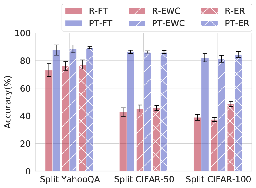
(a) Accuracy ($\uparrow$)

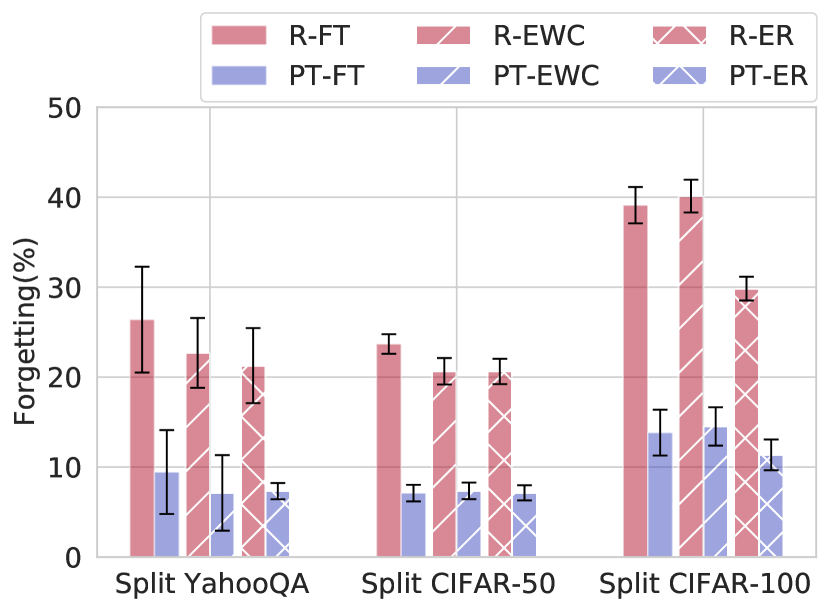
(b) Forgetting ($\downarrow$)

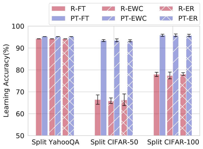
(c) Learning Accuracy ($\uparrow$)

Figure 2: Comparing performance on homogenous tasks (Split YahooQA/ CIFAR-50/ CIFAR-100) across initialization (R: random, PT: pre-trained) and methods (FT: finetune, EWC: elastic weight consolidation, ER: episodic replay) after training on the last task. $\uparrow$ indicates higher is better, $\downarrow$ indicates lower is better. All metrics are averaged over 5 random task sequences. We observe that pre-trained models undergo significantly less forgetting in comparison to randomly initialized models.

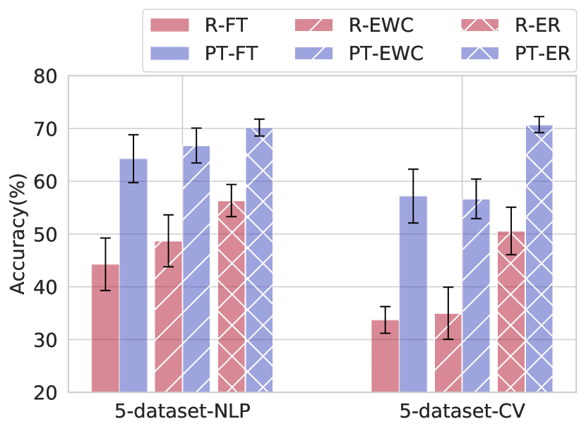
(a) Accuracy ($\uparrow$)

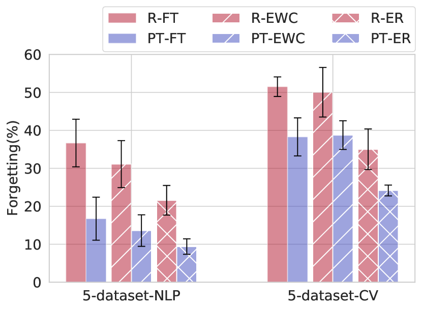
(b) Forgetting ($\downarrow$)

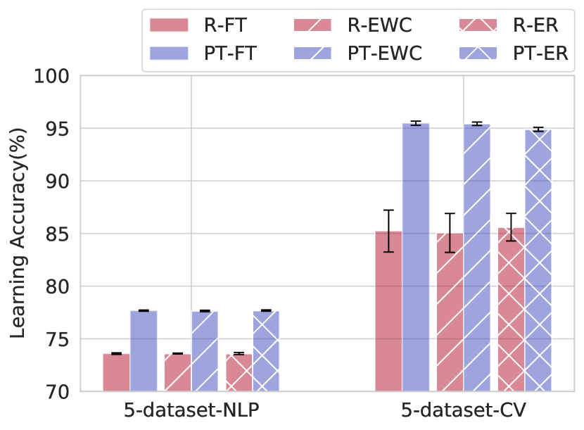
(c) Learning Accuracy ($\uparrow$)

Figure 3: Comparing performance on diverse tasks (5-dataset-NLP/ CV) across initialization (R: random, PT: pre-trained) and methods (FT: finetune, EWC: elastic weight consolidation, ER: episodic replay) after training on the last task. $\uparrow$ indicates higher is better, $\downarrow$ indicates lower is better. All metrics are averaged over 5 task sequences. In comparison to homogenous tasks, we observe that pre-trained models are more susceptible to forgetting when exposed to a diverse sequence of tasks.

3.2 Do pre-trained models undergo similar forgetting on diverse and homogeneous tasks?

From Figure 2(b), we see that ResNet-18-PT does not undergo a significant amount of forgetting when sequentially fine-tuned on Split CIFAR-50, and Split CIFAR-100 (homogenous tasks). On Split CIFAR-50, forgetting is around $7\%$ absolute points. Surprisingly, the competitive ER method also undergoes a similar amount of forgetting, thereby raising a question about the applicability of these data sets when studying forgetting in the context of the pre-trained models. It may be possible to manually cluster tasks based upon semantic closeness, rendering severe interference to make these benchmarks more challenging (Ramasesh et al., 2021). We leave an analysis of pre-trained models on such variants to future work. Given the generic nature of the pre-trained initialization, we ask—what happens when we train the model sequentially on diverse tasks? To answer this question, we conduct experiments on 5-dataset-CV and 5-dataset-NLP. From Figures 2(b), 3(b) (and Table 4), we empirically observe that pre-trained models are more susceptible to forgetting when exposed to diverse tasks in comparison to homogenous tasks. Particularly, DistilBERT-PT/ResNet-18-PT undergoes a $16.73/38.28\%$ absolute points drop in accuracy when trained on 5-dataset-NLP/5-dataset-CV (see Table 4 for exact values). Figures 2(a), 3(a) report average accuracy after training on the last task. We report task-specific results for 5-dataset-NLP/5-dataset-CV in Appendix B.

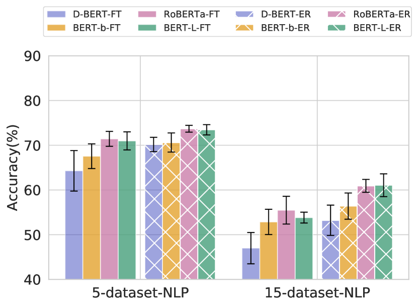
(a) Accuracy ($\uparrow$)

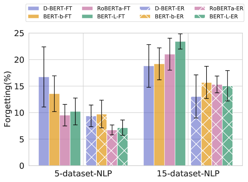
(b) Forgetting ($\downarrow$)

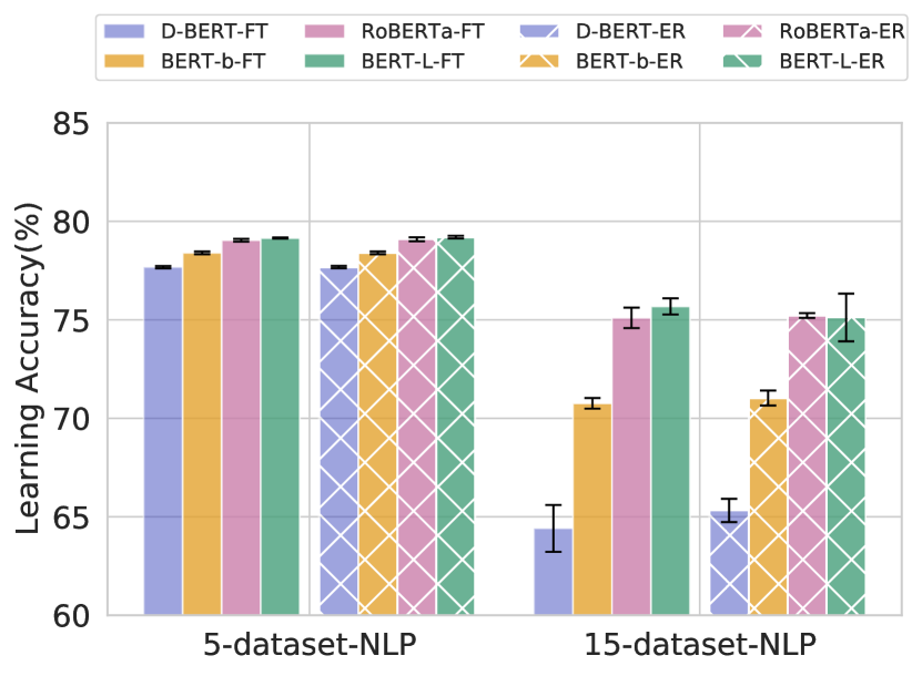
(c) Learning Accuracy ($\uparrow$)

Figure 4: Comparing performance on diverse tasks (5-dataset-NLP/ 15-dataset-NLP) across different pre-trained Transformer models (D-BERT: DistilBERT, BERT-b: BERT-base, RoBERTa: RoBERTa-base, BERT-L: BERT-Large) and methods (FT: finetune, ER: episodic replay) after training on the last task. $\uparrow$ indicates higher is better, $\downarrow$ indicates lower is better. All metrics are averaged over 5 random task sequences. Overall, we observe that larger models and models pre-trained on diverse corpora (RoBERTa-base) undergo less forgetting on both $5$ and $15$ diverse tasks.

3.3 How do different pre-trained initialization affect forgetting?

To examine the impact of varying pre-trained initialization on forgetting, we evaluate different pre-trained Transformer models, DistilBERT (Sanh et al., 2019), BERT (Devlin et al., 2019), RoBERTa (Liu et al., 2019), on text classification tasks. From the previous subsection, we observe that pre-trained models are relatively more susceptible to forgetting on LL of diverse tasks. In response, we conduct a thorough investigation on the 5-dataset-NLP. From Figure 4 (and Table 5), we observe that when keeping the pre-training corpora the same and increasing the capacity of the model – DistilBERT (66M), BERT-base (110M), and BERT-large (336M) – we observe that larger models undergo less forgetting on sequential finetuning of diverse tasks. Further, to understand the impact of the diversity of the pre-training corpora, we compare BERT-base (110M) with RoBERTa-base (125M). We observe that the RoBERTa-base model performs far superior to BERT-base, thus hinting at the necessity of diverse pre-training corpora to alleviate forgetting implicitly. To stress-test these models, we experiment with the 15-dataset-NLP. We observe that by increasing the number of tasks in the sequence, pre-trained models undergo severe forgetting. Surprisingly, the RoBERTa-base model outperforms BERT-Large despite having many fewer parameters. Empirically, we infer that diversity of pre-training corpora plays a vital role in easing forgetting during lifelong learning of diverse tasks.

4 Exploring the Loss Landscape

To better understand how pre-training reduces forgetting, we perform experiments analyzing where models are situated in the loss landscape after training on each task. We denote model parameters after training on task $k$ as $w_{k}$. If we define forgetting as the increase in loss for a given task during training (instead of a decrease in accuracy), Mirzadeh et al. (2020) show that the forgetting can actually be bounded by

$$L_{1}(w_{2})-L_{1}(w_{1})\approx\frac{1}{2}\Delta w^{\top}\nabla^{2}L_{1}(w_{1})\Delta w\leq\frac{1}{2}\lambda_{1}^{max}\lVert{\Delta w}\rVert^{2},$$ (2)

where $L_{1}(w)$ represents the loss on task 1 with parameters $w$, $\Delta w=w_{2}-w_{1}$, and $\lambda_{1}^{max}$ is the largest eigenvalue of $\nabla^{2}L_{1}(w_{1})$. The magnitude of the eigenvalues of $L_{1}(w)$ can be used to characterize the curvature of the loss function (Keskar et al., 2017), and thus $\lambda_{1}^{max}$ can be thought of as a proxy for the flatness of the loss function (lower is flatter). From Equation 2, we can see that the flatter the minima, the less forgetting occurs in the model.

We hypothesize that the one explanation of improvements from pre-training shown in the previous section might be because pre-training leads to a more favorable loss landscape. Specifically, pre-training results in wider/flatter minima for each task. The effect of these wider minima is that the change in weights from learning on future tasks results in a gradual change of the current task loss, thereby reducing forgetting. We verify this idea in two parts. First, we use loss contours and then linearly interpolate between sequential minima to show that the flat loss basins lead to smaller changes in the loss. Next, we compute a sharpness metric to show that pre-training indeed leads to flat loss basins. All models analyzed in this section are sequentially trained using the finetune method.

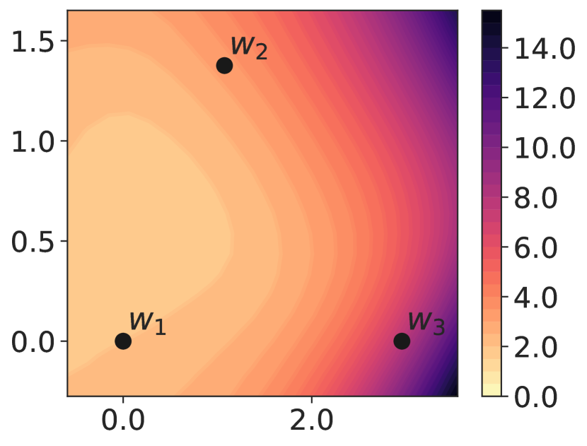
(a) 5-dataset-CV (R)

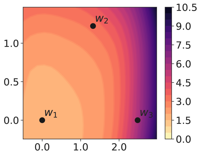
(b) Split CIFAR-50 (R)

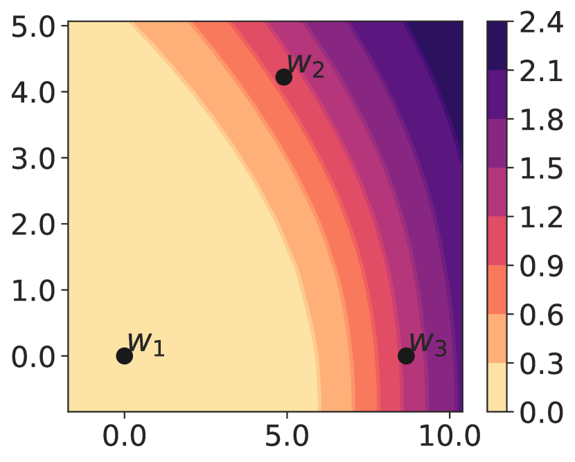
(c) 5-dataset-NLP (R)

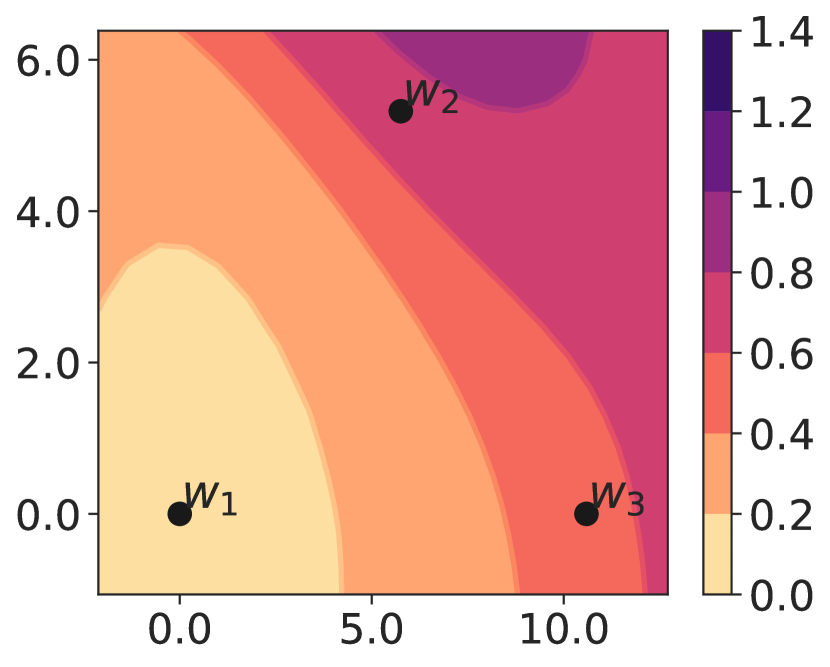
(d) Split YahooQA (R)

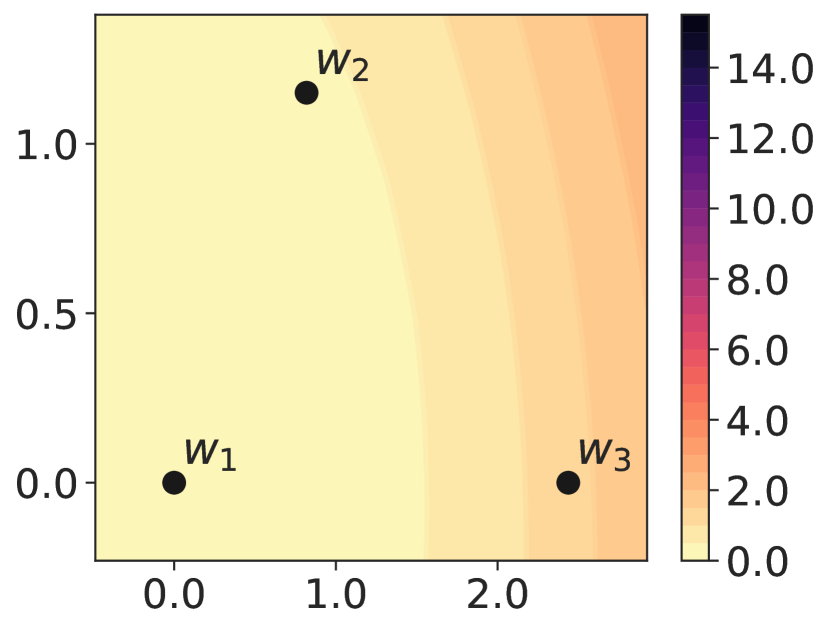
(e) 5-dataset-CV (PT)

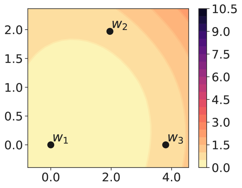
(f) Split CIFAR-50 (PT)

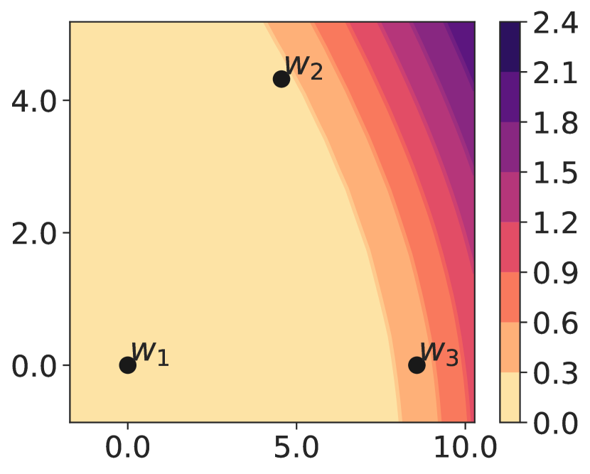
(g) 5-dataset-NLP (PT)

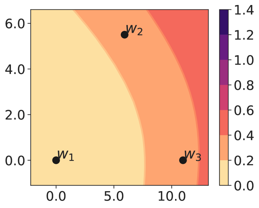
(h) Split YahooQA (PT)

Figure 5: Loss contours for task 1 where w₁, w₂, and w₃ are minima obtained after sequential training on tasks 1, 2, and 3, respectively. The top row visualizes loss contours for randomly initialized models (R) and the bottom row visualizes loss contours for pre-trained models (PT).

4.1 Loss Contour

To better understand the changes in task loss during continual training on a sequence of tasks, we utilize loss contours, which involve linearly interpolating between the continual learning minima. In order to construct a 2D loss contour, we require three points to define two basis vectors. Specifically, we train on tasks 1, 2, and 3 sequentially, resulting in minima represented by w₁, w₂, and w₃, respectively. We designate w₁ as our reference point (0, 0) and calculate $\vec{u}$=w${}_{3}-$w₁ as one basis vector (representing the x-axis in our plots). Additionally, we compute an orthogonal projection $\vec{v}$ of w${}_{2}-$w₁ onto $\vec{u}$, which serves as the second basis vector (representing the y-axis in our plots). Consequently, for any coordinate $(x,y)$ within the 2D loss contour, we derive the corresponding model parameters as w$(x,y)$ = w₁ + $x$.u + $y$.v and compute the validation loss for the task under consideration. In this setup, the distance between any two points on the loss contour reflects the Euclidean distance between the corresponding model parameters.

In Figure 5, we visualize loss contours for the first task across different data set-specific task sequences. For every contour, we plot minima (w₁, w₂, w₃) of the model after continual training on three tasks (T₁, T₂, T₃). As the model is trained continuously on a sequence of tasks, the pre-training initialized model remains largely at the same loss level (for task 1) as compared to the randomly initialized model, despite drifting a comparable distance away from the original model (w₁). For example, in the loss contour for the pre-trained model on 5-dataset-CV (Figure 5(e)), we observe that the model after training on task 2 (w₂) remains at the same loss level as after training on task 1 (w₁) and slightly higher loss level after training on task 3 (w₃). For the randomly initialized model (Figure 5(a)), the Euclidean distance between the model parameter vectors is approximately the same as for the pre-trained model, but the differences in task 1 loss levels are significantly higher. We visualize more instances of loss contours over different task sequences in Appendix C. In summary, we observe that pre-trained models consistently lead to wider loss basins across different data sets (NLP and CV domains), model architectures (ResNet and Transformer), and task sequences (5 random orderings).

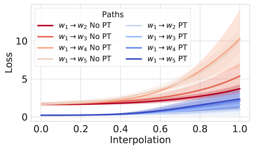
(a) 5-dataset-CV (task 1)

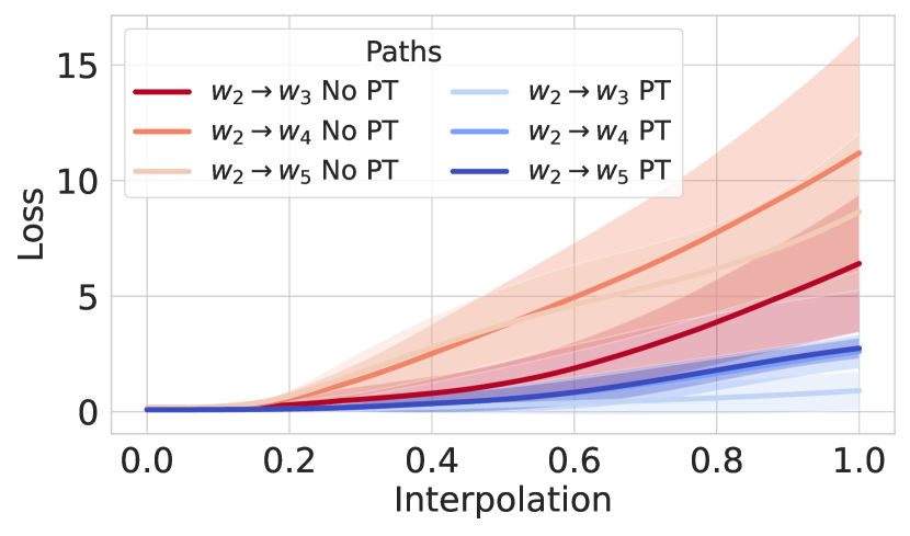
(b) 5-dataset-CV (task 2)

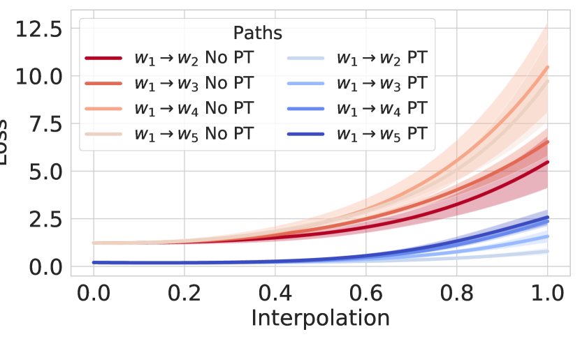
(c) Split CIFAR-50 (task 1)

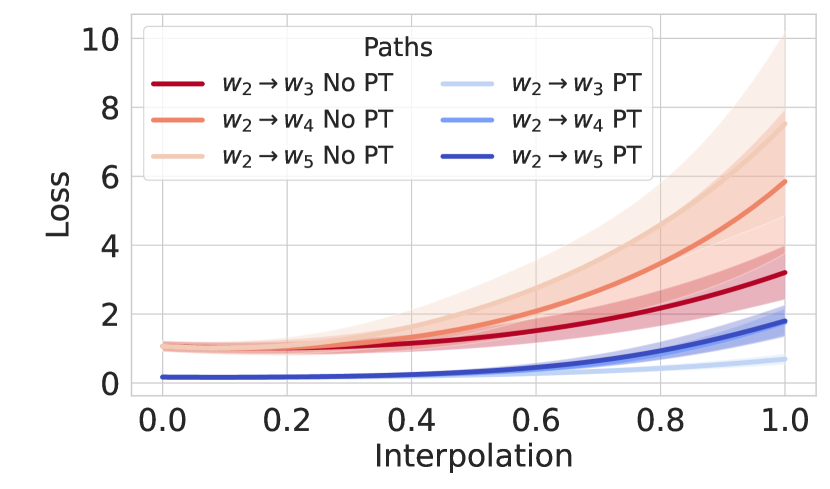
(d) Split CIFAR-50 (task 2)

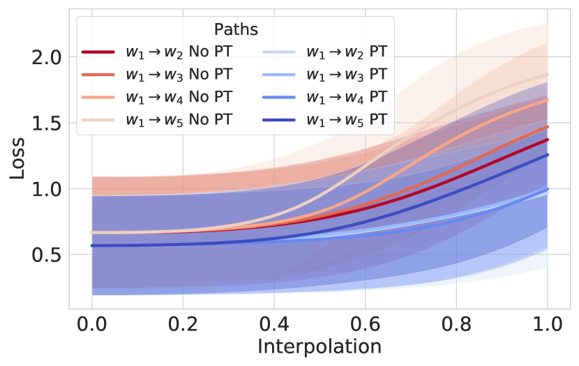
(e) 5-dataset-NLP (task 1)

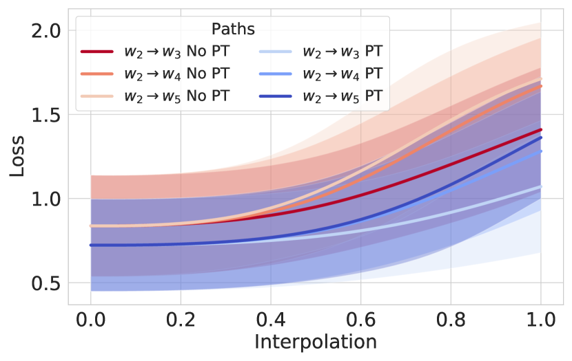
(f) 5-dataset-NLP (task 2)

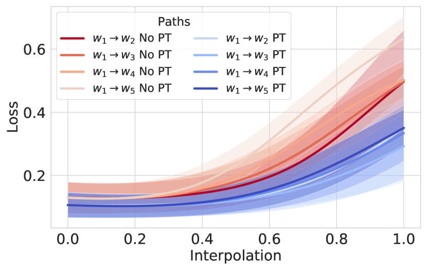
(g) Split YahooQA (task 1)

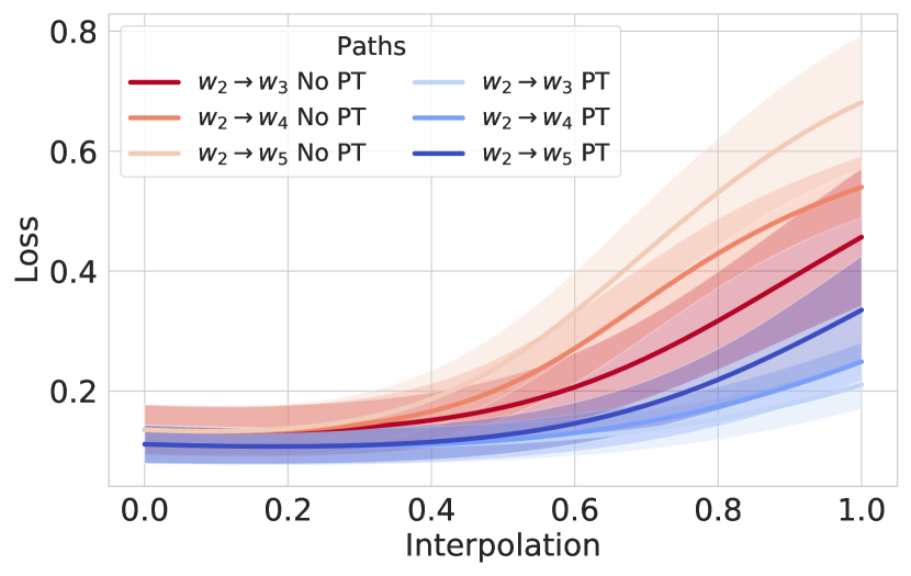
(h) Split YahooQA (task 2)

Figure 6: Linear model interpolation plots for different data sets. The plots for pre-training initialized (PT) models are shown in hues of blue, and the randomly initialized (No PT) models are shown in hues of red. We linearly interpolate between the task 1/ task 2 minimum (w₁/w₂) to the subsequent task minimum (w${}_{i}\rightarrow$ w_j, j > i), tracking the loss in the process. In general, the loss landscape is flatter along these paths for pre-trained initialized models compared to randomly initialized models.

4.2 Linear Model Interpolation

Ideally, to ease forgetting during sequential training of tasks, loss on previous tasks should undergo minimal change. This desideratum would be satisfied if a previous task minimum lands in a flat loss region and subsequent task minima also remained in that flat loss region. To probe this behavior, we linearly interpolate between w₁ (w₂) and subsequent task minima, tracking the (validation) loss on task 1 (task 2). This probe can be interpreted as viewing a slice of the loss contours in Figure 5 along the linear trajectory connecting w₁ (w₂) to a subsequent minimum. In Figure 6, we visualize the results from linear interpolation with the first row for task 1 and the second row for task 2. The plots for pre-training initialized models are shown in hues of blue, and the randomly initialized models are shown in hues of red. These plots illustrate that the pre-training initialized models experience a much more gradual increase in loss compared to the randomly initialized models, even when interpolating to minima after training on several tasks. Moreover, these results hold for task 2 as well, thereby reinforcing that pre-training initialized models lead to flat minima even for subsequent tasks in a sequence.

	w/o PT	w/ PT	w/o PT	w/ PT
	$\epsilon=5\times 10^{-4}$		$\epsilon=10^{-3}$
5-dataset-CV	$2.1_{0.6}$	$0.1_{0.0}$	$5.7_{1.6}$	$0.2_{0.0}$
Split CIFAR-50	$2.3_{0.7}$	$0.2_{0.1}$	$6.1_{1.5}$	$0.4_{0.1}$
Split CIFAR-100	$2.3_{0.6}$	$0.1_{0.0}$	$5.9_{1.3}$	$0.2_{0.1}$
	$\epsilon=5\times 10^{-5}$		$\epsilon=10^{-4}$
5-dataset-NLP	$32.7_{1.2}$	$28.3_{1.2}$	$213.6_{11.5}$	$129.0_{10.5}$
Split YahooQA	$10.4_{0.4}$	$8.8_{0.4}$	$53.2_{7.0}$	$43.0_{4.2}$

Table 3: Average sharpness value (lower value corresponds to flat loss basin) of task minima. ResNet-18-PT/DistilBERT-PT (w/ PT) has lower average sharpness in comparison to ResNet-18-R/DistilBERT-R (w/o PT). Pre-training reduces the sharpness of minima for each task in training by an order of magnitude.

4.3 Sharpness

As discussed earlier, the flatness of the minima can be estimated based upon the magnitude of eigenvalues of $\nabla^{2}L(w)$. However, computing these eigenvalues is computationally expensive. Therefore, Keskar et al. (2017) introduces a sensitivity measure, termed sharpness metric, as a computationally feasible alternative to computing eigenvalues. The sharpness metric estimates the flatness by computing the maximum value of the loss function $L$ in a constrained neighborhood around the minima. Given that the maximization process can be inaccurate, Keskar et al. (2017) suggests performing maximization in a random subspace $\mathbb{R}^{p}$ of the entire parameter space $\mathbb{R}^{n}$, specified by a projection matrix $A\in\mathbb{R}^{n\times p}$. For our experiments, we randomly sample our matrix $A$ and set $p=100$ as in Keskar et al. (2017). The neighborhood maximization region ($C_{\epsilon}$) is defined as

$$C_{\epsilon}=\{z\in\mathbb{R}^{p}:-\epsilon(|(A^{+}w)_{i}|+1)\leq z_{i}\leq\epsilon(|(A^{+}w)_{i}|+1);\forall i\in\{1\dots p\}\},$$ (3)

where $A^{+}$ is the pseudo inverse of $A$, $w$ is the parameter vector and $\epsilon$ is a hyperparameter controlling the size of the neighborhood. Formally, the sharpness metric is defined as follows

$$\phi_{w,L}\coloneqq\frac{(\max_{z\in C_{\epsilon}}L(w+Az))-L(w)}{1+L(w)}\times 100,$$ (4)

where $L(w)$ denotes the loss function with parameters $w$. According to Keskar et al. (2017), the sharpness metric is closely related to the spectrum $\nabla^{2}L(w)$, therefore acts as a proxy measure for $\lambda_{1}^{max}$ in Equation 2. After training on each task, we evaluate the minimum reached by the model for its sharpness (alternatively flatness). We average the sharpness values across all tasks in a given task sequence and report the mean and standard deviation across 5 random task orderings. In Appendix A, we provide implementation details about the sharpness metric.

In Table 3, we report sharpness values for ResNet-18 on 5-dataset-CV, Split CIFAR-50/CIFAR-100 for $\epsilon\in\{5e^{-4},1e^{-3}\}$ and DistilBERT on 5-dataset-NLP and Split YahooQA data sets for $\epsilon\in\{5e^{-5},1e^{-4}\}$. We see that for all data sets, the average sharpness value for the pre-trained initialized models is significantly lower than for the randomly initialized models, validating the relative flatness of the task minima in the case of pre-trained models.

5 Lifelong Learning with Sharpness Aware Minimization (SAM)

In the previous section, we looked at the role of initialization in alleviating forgetting. Specifically, pre-trained initializations favor flat loss basins and implicitly mitigate forgetting to some extent. On the other hand, Mirzadeh et al. (2020) suggests modifying the training regime by varying learning rate decay, batch size, and dropout regularization such that inherent noise in the stochastic gradients leads to flat basins in the loss landscape. However, the procedure for tuning these hyperparameters is ill-defined for lifelong learning, thereby rendering their strategy less helpful. Furthermore, the suggested hyperparameter sweep is expensive (e.g., $48$ separate runs just for one data set) and does not transfer across different architectures and data sets. Motivated by these shortcomings, we pose a question—What if we modify the optimization dynamics by explicitly seeking flat loss basins during lifelong learning of the model? Alternatively, what if we jointly optimize the sharpness metric and the current task loss? Towards this objective, we employ the Sharpness-Aware Minimization (SAM) procedure (Foret et al., 2021) that seeks parameters that lie in the neighborhoods having uniformly low loss values by jointly minimizing the task loss value and sharpness metric. SAM defines the sharpness of the loss function $L$ at parameters $w$ as

$$\max_{||\epsilon||_{2}\leq\rho}L(w+\epsilon)-L(w),$$ (5)

where maximization region is an $\ell^{p}$ ball with radius $\rho$ for $p=2$ in Equation 5. SAM problem can be defined in terms of the following minimax optimization

$$\min_{w}\max_{||\epsilon||_{2}\leq\rho}L(w+\epsilon)+\lambda||w||_{2}^{2}.$$ (6)

The gradient of the result of the maximization problem can be approximated as

$$\nabla_{w}\max_{||\epsilon||_{2}\leq\rho}L(w+\epsilon)\approx\nabla_{w}L(w)\Big{\rvert}_{w+\hat{\epsilon}(w)}+\frac{d\hat{\epsilon}(w)}{dw}\nabla_{w}L(w)\Big{\rvert}_{w+\hat{\epsilon}(w)},$$ (7)

where

$$\hat{\epsilon}(w)=\rho\operatorname{sign}\big{(}\nabla_{w}L(w)\big{)}\Bigg{(}\frac{\big{\lvert}\nabla_{w}L(w)\big{\rvert}}{\lVert\nabla_{w}L(w)\rVert_{2}}\Bigg{)}.$$ (8)

To make the optimization simpler, the second-order term in the gradient is dropped, leaving us with

$$\nabla_{w}\max_{||\epsilon||_{2}\leq\rho}L(w+\epsilon)\approx\nabla_{w}L(w)\Big{\rvert}_{w+\hat{\epsilon}(w)}.$$ (9)

For the complete derivation of this gradient, we defer readers to Foret et al. (2021).

	w/o PT (ResNet-18-R/DistilBERT-R)			w/ PT (ResNet-18-PT/DistilBERT-PT)
	Accuracy($\uparrow$)	Forgetting($\downarrow$)	LearnAcc($\uparrow$)	Accuracy($\uparrow$)	Forgetting($\downarrow$)	LearnAcc($\uparrow$)
Split YahooQA
FT	$73.1_{4.7}$	$26.4_{5.9}$	$94.2_{0.0}$	$87.7_{3.7}$	$9.5_{4.7}$	$95.2_{0.0}$
FT w/ SAM	$73.5_{4.0}$	$25.9_{5.0}$	$94.2_{0.0}$	$88.5_{2.8}$	$8.4_{3.5}$	$95.2_{0.0}$
EWC	$76.1_{3.1}$	$22.7_{3.9}$	$94.2_{0.0}$	$89.5_{3.4}$	$7.1_{4.2}$	$95.2_{0.0}$
ER	$77.2_{3.3}$	$21.3_{4.2}$	$94.2_{0.0}$	$\mathbf{89.4_{0.7}}$	$\mathbf{7.3_{0.9}}$	$95.2_{0.0}$
ER w/ SAM	$\mathbf{77.5_{1.4}}$	$\mathbf{20.9_{1.8}}$	$94.2_{0.0}$	$89.0_{0.7}$	$7.8_{0.9}$	$95.2_{0.0}$
5-dataset-NLP
FT	$44.3_{5.0}$	$36.7_{6.3}$	$73.6_{0.1}$	$64.3_{4.5}$	$16.7_{5.7}$	$77.7_{0.1}$
FT w/ SAM	$46.0_{5.0}$	$34.3_{6.3}$	$73.4_{0.1}$	$66.4_{2.8}$	$13.9_{3.5}$	$77.6_{0.1}$
EWC	$48.7_{4.9}$	$31.1_{6.2}$	$73.6_{0.0}$	$66.8_{3.3}$	$13.6_{4.2}$	$77.6_{0.1}$
ER	$\mathbf{56.3_{3.1}}$	$\mathbf{21.6_{3.9}}$	$73.6_{0.1}$	$70.2_{1.6}$	$9.4_{2.0}$	$77.7_{0.1}$
ER w/ SAM	$56.3_{3.9}$	$21.5_{5.0}$	$73.4_{0.1}$	$\mathbf{71.1_{1.2}}$	$\mathbf{8.1_{1.5}}$	$77.5_{0.0}$
Split CIFAR-50
FT	$42.8_{3.1}$	$23.7_{1.1}$	$66.4_{2.1}$	$86.3_{1.2}$	$7.1_{0.9}$	$93.4_{0.5}$
FT w/ NSGD	$46.4_{2.3}$	$24.7_{1.6}$	$71.1_{0.9}$	$86.5_{0.9}$	$7.4_{0.7}$	$93.5_{0.3}$
FT w/ SAM	$50.3_{2.2}$	$15.0_{2.1}$	$65.3_{1.2}$	$\mathbf{90.5_{1.1}}$	$\mathbf{4.2_{1.0}}$	$94.7_{0.4}$
Stable SGD	$46.0_{2.3}$	$12.1_{0.4}$	$58.1_{2.5}$	$84.1_{1.9}$	$5.2_{1.6}$	$89.2_{0.7}$
EWC	$45.3_{2.5}$	$20.7_{1.5}$	$65.9_{1.3}$	$86.2_{0.9}$	$7.4_{0.9}$	$93.5_{0.7}$
A-GEM	$47.3_{2.7}$	$21.1_{2.0}$	$68.4_{0.7}$	$87.3_{1.0}$	$6.2_{0.6}$	$93.4_{0.4}$
ER	$45.8_{1.8}$	$20.6_{1.4}$	$66.4_{2.7}$	$86.2_{1.1}$	$7.1_{0.8}$	$93.3_{0.5}$
ER w/ SAM	$50.8_{0.5}$	$16.9_{0.9}$	$67.6_{0.7}$	$88.4_{1.3}$	$6.0_{1.1}$	$94.4_{0.3}$
MC-SGD	$59.0_{2.3}$	$5.4_{1.3}$	$63.7_{1.8}$	$86.5_{0.9}$	$4.1_{0.5}$	$90.4_{0.6}$
MC-SGD w/ SAM	$\mathbf{59.1_{2.9}}$	$\mathbf{5.2_{1.7}}$	$63.9_{2.1}$	$87.9_{0.7}$	$3.8_{0.2}$	$91.7_{0.7}$
5-dataset-CV
FT	$33.7_{2.5}$	$51.5_{2.6}$	$85.2_{2.0}$	$57.2_{5.1}$	$38.3_{5.0}$	$95.5_{0.2}$
FT w/ NSGD	$35.8_{3.7}$	$52.4_{3.3}$	$88.2_{1.3}$	$56.6_{5.1}$	$39.0_{4.9}$	$95.6_{0.3}$
FT w/ SAM	$47.6_{3.8}$	$40.6_{4.0}$	$88.2_{1.3}$	$70.4_{4.4}$	$25.6_{4.4}$	$96.0_{0.1}$
Stable SGD	$50.2_{7.0}$	$40.3_{7.8}$	$90.5_{1.0}$	$71.3_{2.7}$	$20.5_{2.5}$	$91.9_{0.8}$
EWC	$35.0_{4.9}$	$50.1_{6.5}$	$85.1_{1.9}$	$56.7_{3.8}$	$38.8_{3.8}$	$95.4_{0.2}$
A-GEM	$46.1_{6.8}$	$39.5_{7.1}$	$85.2_{2.5}$	$72.0_{2.3}$	$23.0_{2.3}$	$95.0_{0.2}$
ER	$50.6_{4.5}$	$35.0_{5.4}$	$85.6_{1.3}$	$70.7_{1.5}$	$24.2_{1.4}$	$94.9_{0.2}$
ER w/ SAM	$60.3_{3.9}$	$27.3_{4.1}$	$87.6_{1.3}$	$77.4_{3.9}$	$18.2_{3.9}$	$95.6_{0.2}$
MC-SGD	$71.3_{5.9}$	$21.3_{5.7}$	$92.6_{0.3}$	$81.9_{2.6}$	$13.3_{2.6}$	$95.2_{0.3}$
MC-SGD w/ SAM	$\mathbf{72.7_{7.8}}$	$\mathbf{19.9_{7.6}}$	$92.6_{0.4}$	$\mathbf{87.1_{1.6}}$	$\mathbf{8.5_{1.7}}$	$95.5_{0.2}$
Split CIFAR-100
FT	$38.9_{2.2}$	$39.1_{2.0}$	$78.0_{1.0}$	$82.0_{3.0}$	$13.8_{2.6}$	$95.8_{0.5}$
FT w/ NSGD	$40.2_{3.5}$	$41.7_{3.2}$	$81.9_{0.8}$	$79.8_{3.4}$	$16.2_{3.1}$	$96.0_{0.6}$
FT w/ SAM	$48.9_{4.8}$	$28.5_{5.0}$	$77.5_{0.9}$	$88.3_{1.7}$	$8.6_{1.3}$	$96.9_{0.6}$
Stable SGD	$52.9_{1.7}$	$21.0_{2.0}$	$73.8_{1.5}$	$86.6_{2.2}$	$5.5_{1.5}$	$91.8_{0.7}$
EWC	$37.4_{1.5}$	$40.1_{1.8}$	$77.5_{1.5}$	$81.3_{2.5}$	$14.5_{2.1}$	$95.8_{0.6}$
A-GEM	$46.8_{3.5}$	$32.0_{3.8}$	$78.8_{1.0}$	$84.0_{1.6}$	$11.7_{1.0}$	$95.7_{0.7}$
ER	$48.6_{1.9}$	$29.8_{1.3}$	$78.1_{0.7}$	$84.4_{2.2}$	$11.4_{1.7}$	$95.8_{0.5}$
ER w/ SAM	$60.5_{0.5}$	$20.9_{0.7}$	$81.4_{0.7}$	$88.4_{0.7}$	$8.6_{0.2}$	$96.7_{0.5}$
MC-SGD	$62.2_{2.4}$	$13.3_{1.8}$	$75.2_{0.7}$	$84.7_{2.4}$	$8.5_{1.8}$	$93.0_{0.7}$
MC-SGD w/ SAM	$\mathbf{65.1_{1.1}}$	$\mathbf{10.4_{1.1}}$	$75.4_{1.0}$	$\mathbf{89.0_{1.7}}$	$\mathbf{5.3_{1.1}}$	$94.2_{0.6}$

Table 4: Comparing performance in terms of accuracy($\%$), forgetting($\%$), and learning accuracy ($\%$) across methods after training on the last task (all metrics are averaged over 5 random task sequences). $\uparrow$ indicates higher is better, $\downarrow$ indicates lower is better. Augmenting the FT baseline with SAM results in performance competitive with state-of-the-art methods, and augmenting the ER or MC-SGD method with SAM often outperforms state-of-the-art methods demonstrating SAM as a valuable addition to current lifelong learning methods.

	5-dataset-NLP			15-dataset-NLP
	Accuracy($\uparrow$)	Forgetting($\downarrow$)	LearnAcc($\uparrow$)	Accuracy($\uparrow$)	Forgetting($\downarrow$)	LearnAcc($\uparrow$)
DistilBERT
FT	$64.3_{4.5}$	$16.7_{5.7}$	$77.7_{0.1}$	$47.0_{3.5}$	$18.8_{4.0}$	$64.4_{1.2}$
FT w/ SAM	$66.4_{2.8}$	$13.9_{3.5}$	$77.6_{0.1}$	$47.5_{3.1}$	$16.5_{3.8}$	$62.5_{0.8}$
ER	$70.2_{1.6}$	$9.4_{2.0}$	$77.7_{0.1}$	$53.2_{3.4}$	$13.1_{4.1}$	$65.3_{0.6}$
ER w/ SAM	$\mathbf{71.1_{1.2}}$	$\mathbf{8.1_{1.5}}$	$77.5_{0.0}$	$\mathbf{53.5_{2.0}}$	$\mathbf{11.0_{3.1}}$	$63.1_{1.0}$
T5-Small
FT	$65.9_{2.8}$	$12.6_{3.7}$	$76.0_{0.2}$	$44.9_{3.2}$	$21.9_{3.0}$	$65.2_{0.6}$
FT w/ SAM	$66.4_{2.3}$	$11.9_{3.0}$	$75.9_{0.3}$	$46.6_{3.0}$	$19.3_{3.0}$	$64.4_{0.7}$
ER	$69.4_{1.0}$	$8.2_{1.2}$	$75.9_{0.2}$	$48.1_{1.3}$	$18.9_{1.0}$	$65.5_{0.8}$
ER w/ SAM	$\mathbf{69.9_{0.2}}$	$\mathbf{7.5_{0.1}}$	$75.9_{0.2}$	$\mathbf{48.6_{1.6}}$	$\mathbf{17.4_{1.2}}$	$64.5_{0.7}$
BERT-base
FT	$67.6_{2.8}$	$13.6_{3.4}$	$78.4_{0.1}$	$52.9_{2.8}$	$19.2_{3.0}$	$70.8_{0.3}$
FT w/ SAM	$70.8_{2.1}$	$9.5_{2.5}$	$78.4_{0.1}$	$55.1_{2.6}$	$16.4_{3.2}$	$70.4_{0.7}$
ER	$70.6_{2.1}$	$9.7_{2.6}$	$78.4_{0.1}$	$56.4_{2.9}$	$15.7_{3.0}$	$71.0_{0.4}$
ER w/ SAM	$\mathbf{73.0_{1.5}}$	$\mathbf{6.9_{1.9}}$	$78.5_{0.1}$	$\mathbf{57.8_{1.9}}$	$\mathbf{13.7_{1.9}}$	$70.5_{0.5}$
RoBERTa-base
FT	$71.4_{1.7}$	$9.5_{2.0}$	$79.0_{0.1}$	$55.5_{3.1}$	$21.0_{3.0}$	$75.1_{0.5}$
FT w/ SAM	$72.6_{1.2}$	$7.8_{1.5}$	$78.8_{0.0}$	$57.8_{1.7}$	$15.4_{1.9}$	$72.1_{1.4}$
ER	$73.7_{0.8}$	$6.7_{0.9}$	$79.1_{0.1}$	$60.9_{1.4}$	$15.3_{1.6}$	$75.2_{0.1}$
ER w/ SAM	$\mathbf{74.3_{0.6}}$	$\mathbf{5.7_{0.8}}$	$78.9_{0.0}$	$\mathbf{62.1_{1.5}}$	$\mathbf{12.2_{2.1}}$	$73.3_{0.8}$
BERT-Large
FT	$71.0_{2.0}$	$10.2_{2.5}$	$79.2_{0.0}$	$53.8_{1.2}$	$23.4_{1.4}$	$75.7_{0.4}$
FT w/ SAM	$73.7_{1.3}$	$6.9_{1.6}$	$79.2_{0.0}$	$58.7_{3.4}$	$17.1_{4.3}$	$74.6_{2.2}$
ER	$73.5_{1.2}$	$7.2_{1.4}$	$79.2_{0.1}$	$61.1_{2.6}$	$15.1_{2.9}$	$75.1_{1.2}$
ER w/ SAM	$\mathbf{74.6_{0.6}}$	$\mathbf{5.7_{0.8}}$	$79.2_{0.1}$	$\mathbf{61.7_{1.3}}$	$\mathbf{13.7_{2.8}}$	$74.5_{1.5}$

Table 5: Comparing performance in terms of average accuracy (%), forgetting (%), and learning accuracy (%) across pre-trained Transformers after continual learning the last task. $\uparrow$ indicates higher is better, $\downarrow$ indicates lower is better. All metrics are averaged over 5 random task sequences. Overall, we observe that models pre-trained on diverse corpora (RoBERTa-base) undergo less forgetting on both $5$ and $15$ diverse tasks. Furthermore, augmenting the FT and ER methods with SAM often outperforms state-of-the-art methods.

In Tables 4 and 5, we report the results with the discussed SAM procedure. We see that SAM results in a consistent improvement in performance over non-SAM counterparts. Simply augmenting SAM with the finetune method (FT w/ SAM) results in a competitive baseline, sometimes outperforming state-of-the-art baselines like ER (Chaudhry et al., 2019), Stable SGD (Mirzadeh et al., 2020) and MC-SGD (Mirzadeh et al., 2021) (see Table 4, Split CIFAR-50 w/PT ResNet-18-PT). Note SAM requires minimal hyper-parameter tuning (we set $\rho=0.05$ to the default value for all our CV experiments). Since SAM is just a modification to the optimization procedure, we propose augmenting it with existing state-of-the-art continual learning methods like ER (Chaudhry et al., 2019) and MC-SGD (Mirzadeh et al., 2021).

From Table 4, MC-SGD w/ SAM outperforms all existing baselines in terms of overall accuracy and forgetting across all considered CV benchmarks (Split CIFAR-50, Split CIFAR-100, and 5-dataset-CV) when evaluated in the context of random as well as pre-trained initialized models. From Tables 4 and 5, ER w/ SAM results in a method that outperforms all existing baselines in terms of overall accuracy and forgetting across all NLP benchmarks. Furthermore, in Table 5, we present the results obtained with T5-Small (v1.1) (Raffel et al., 2020) on the 5-dataset-NLP and 15-dataset-NLP benchmarks. Consistent with encoder-only models such as DistilBERT, BERT, and RoBERTa, we observe that FT w/ SAM and ER w/ SAM outperform their non-SAM counterparts on the encoder-decoder architecture. This finding highlights the broad applicability of SAM across different model architectures, including both encoder-only and encoder-decoder setups. To summarize, SAM serves as a valuable addition to current continual learning methods and can be seamlessly incorporated to enhance overall performance.

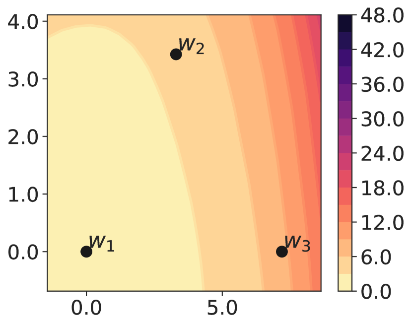
(a) FT (T1)

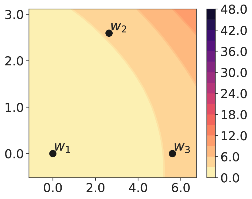
(b) FT w/ SAM (T1)

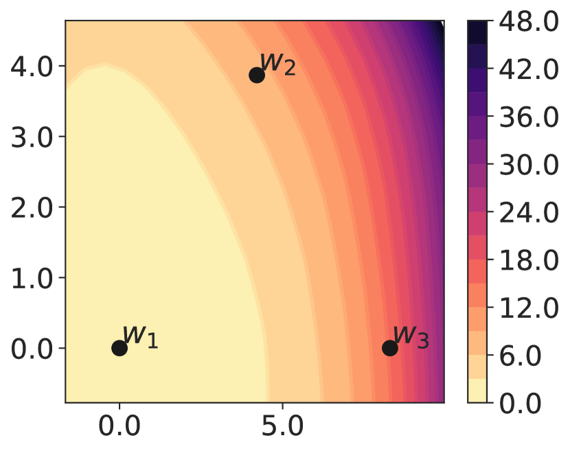
(c) ER (T1)

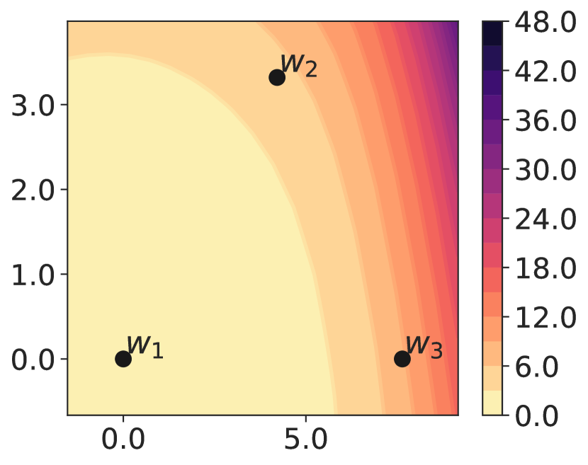
(d) ER w/ SAM (T1)

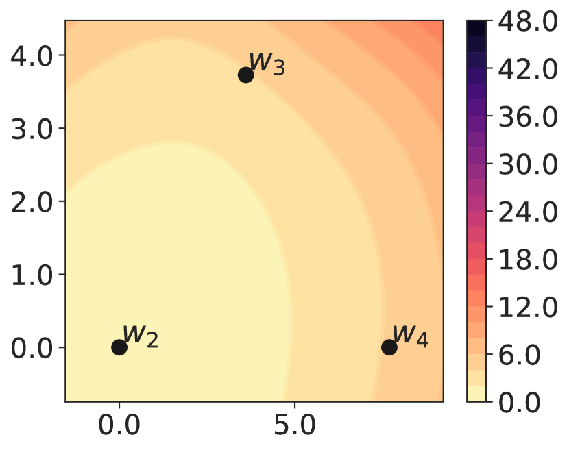
(e) FT (T2)

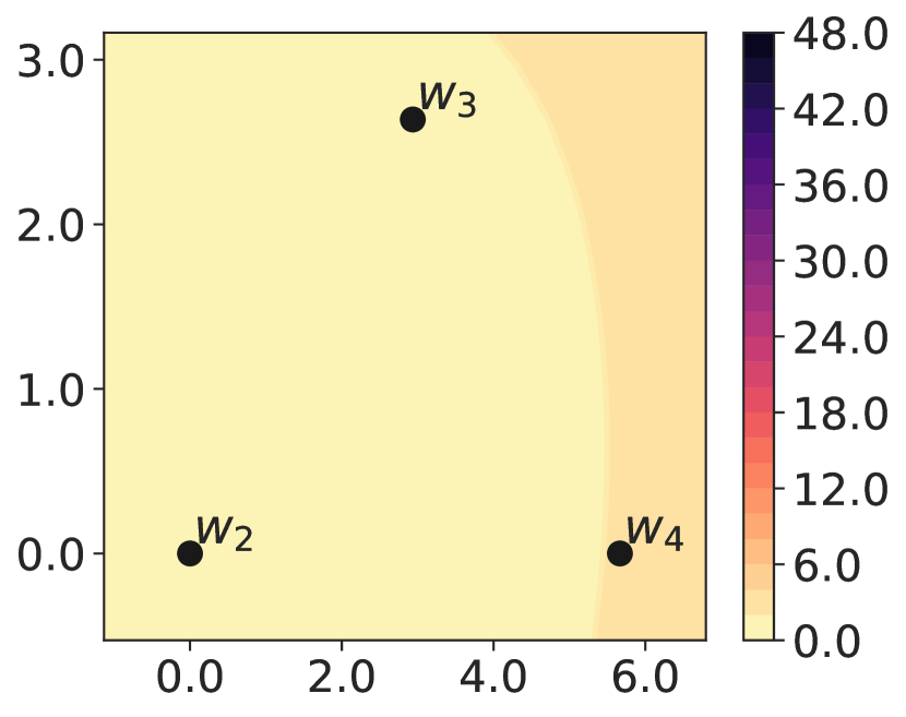
(f) FT w/ SAM (T2)

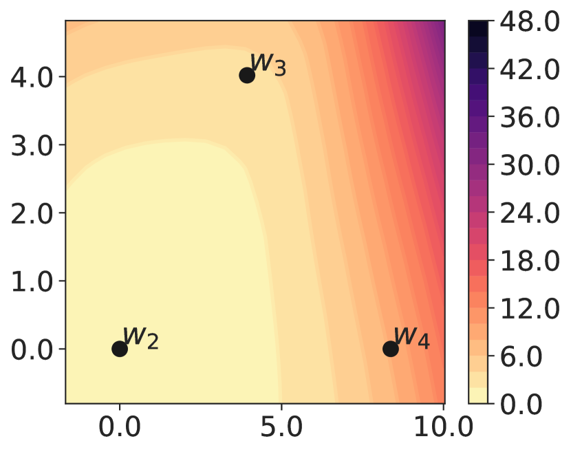
(g) ER (T2)

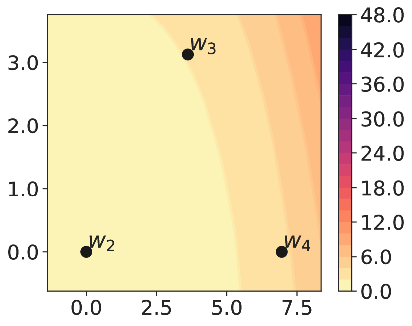
(h) ER w/ SAM (T2)

Figure 7: Loss contours for task 1 (T1) and task 2 (T2) of Split CIFAR-50. The top row visualizes loss contours for task 1 where w₁, w₂, and w₃ are minima obtained after sequential training on tasks 1, 2, and 3, respectively. Similarly, the bottom row visualizes loss contours for task 2 after sequential training on tasks 2, 3, and 4. All of the above models start with random weights. SAM (FT w/ SAM, ER w/ SAM) leads to wide task minima compared to finetune (FT) and ER methods.

5.1 Loss Contours and Sharpness with SAM

In order to understand the effectiveness of the SAM, we visualize the loss contours and compute the sharpness metric (Equation 4). We plot loss contours for task 1/ task 2 of Split CIFAR-50 (Figure 7) and 5-dataset-CV (Figure 8), under continual training from randomly initialized weights, and compare them across four different methods: FT, FT w/ SAM, ER, and ER w/ SAM. We show that SAM (FT w/ SAM and ER w/ SAM) leads to wide task minima (task 1/ task 2) across both data sets as compared to FT and ER methods. Moreover, from Table 4 for ResNet-18-R (w/o PT) initialization, we see that for Split CIFAR-50, FT w/ SAM (15.0), ER w/ SAM (16.9), and MC-SGD w/ SAM (5.2) undergoes lesser forgetting than FT (23.7), ER (20.6), and MC-SGD (5.4) methods, respectively. These results convincingly demonstrate the effectiveness of SAM when used with vanilla FT, ER, and/ or MC-SGD methods. Similarly, we see that for 5-dataset-CV, MC-SGD w/ SAM (19.9) undergoes lesser forgetting than ER w/ SAM (27.3) and FT w/ SAM (40.6), which in turn significantly improves over FT (51.5). Next, we compare the loss contours between FT and ER methods and do not notice any stark difference in terms of flatness. However, in the presence of SAM, qualitatively we see that ER w/ SAM (Figures 8(d), 8(h)) leads to a flat loss basin in comparison to FT w/ SAM (Figures 8(b), 8(f)).

We compute the sharpness metric for FT and FT w/ SAM methods. In Table 6 we report sharpness metrics for 5-dataset-CV and Split CIFAR-50. We see that the SAM significantly reduces the sharpness in the case of randomly initialized models. Concretely, on the 5-dataset-CV, we see that the sharpness value (for $\epsilon=5$x$10^{-4}$ ) decreases from 2.1 (FT) to 0.7 (FT w/ SAM). Similarly, on the Split CIFAR-50, we see a drop from 2.3 (FT) to 0.7 (FT w/ SAM). These results validate that SAM indeed leads to flat minima, therefore, explaining the superior performance (in terms of average accuracy and forgetting) of SAM optimization procedure over baseline.

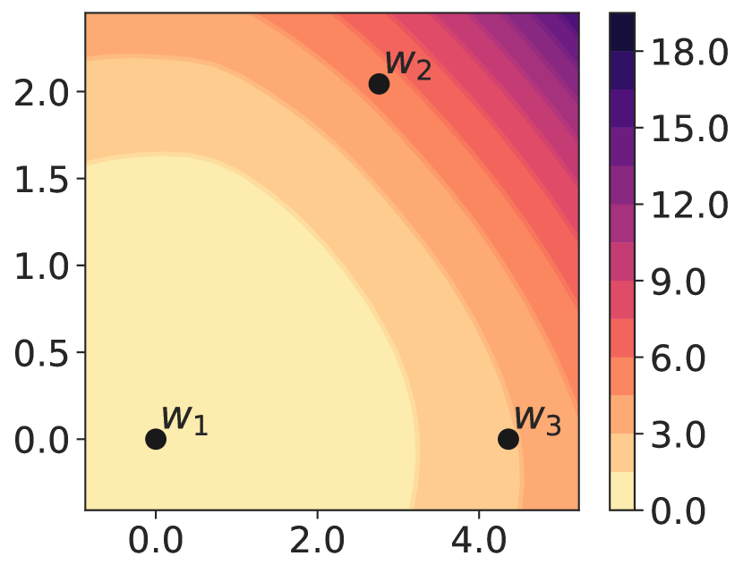
(a) FT (T1)

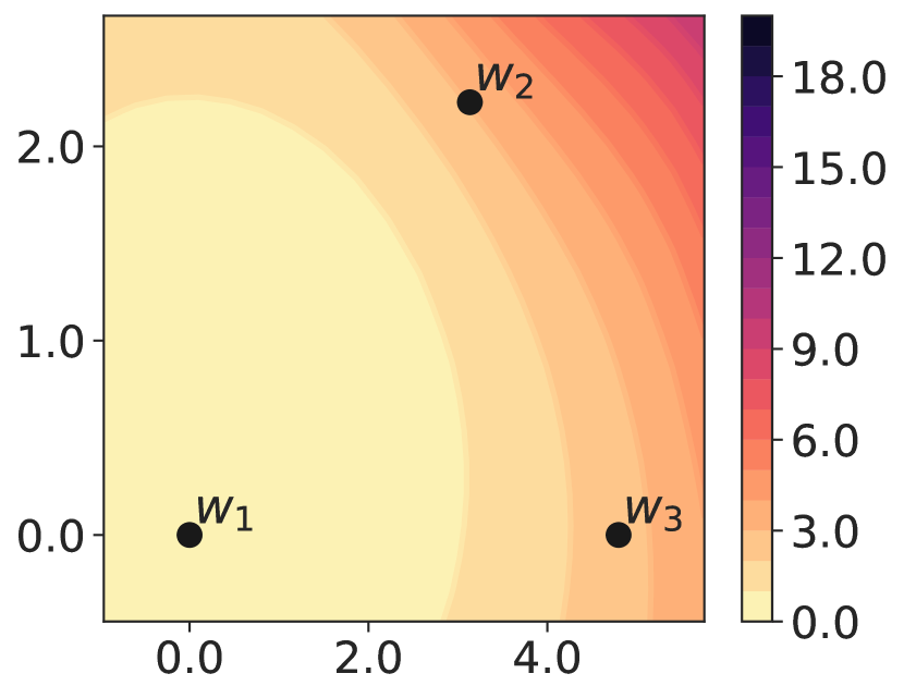
(b) FT w/ SAM (T1)

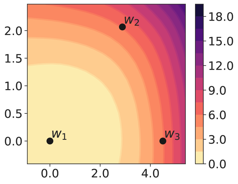
(c) ER (T1)

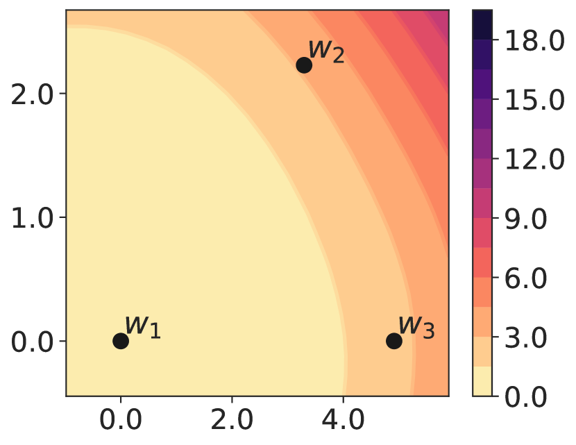
(d) ER w/ SAM (T1)

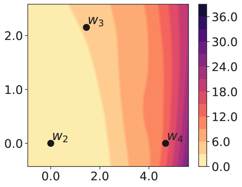
(e) FT (T2)

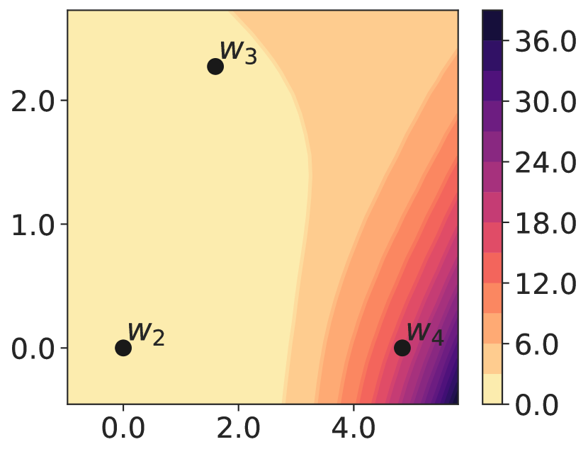
(f) FT w/ SAM (T2)

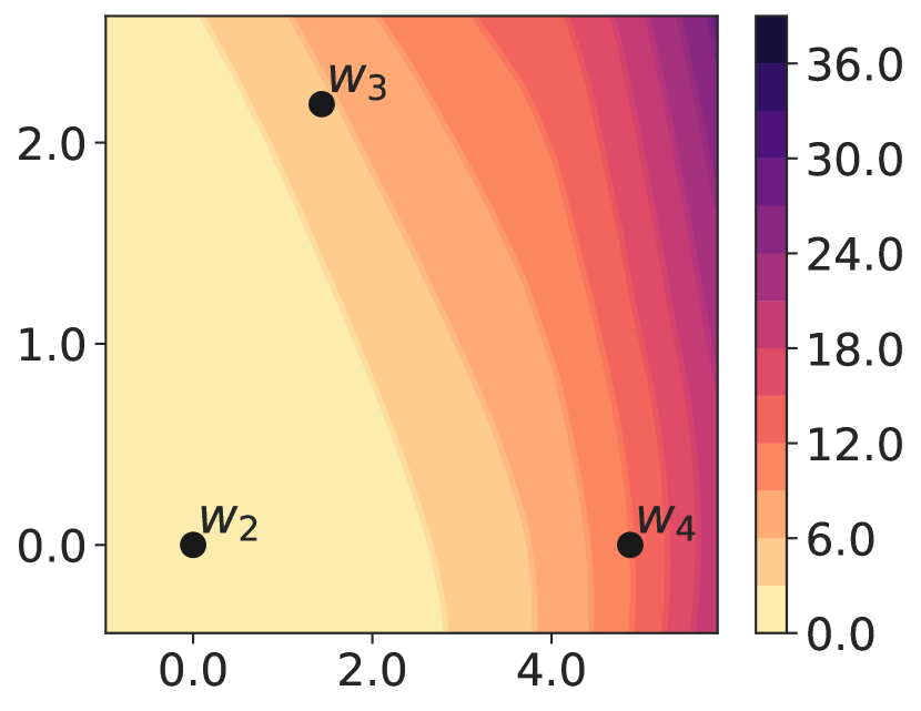
(g) ER (T2)

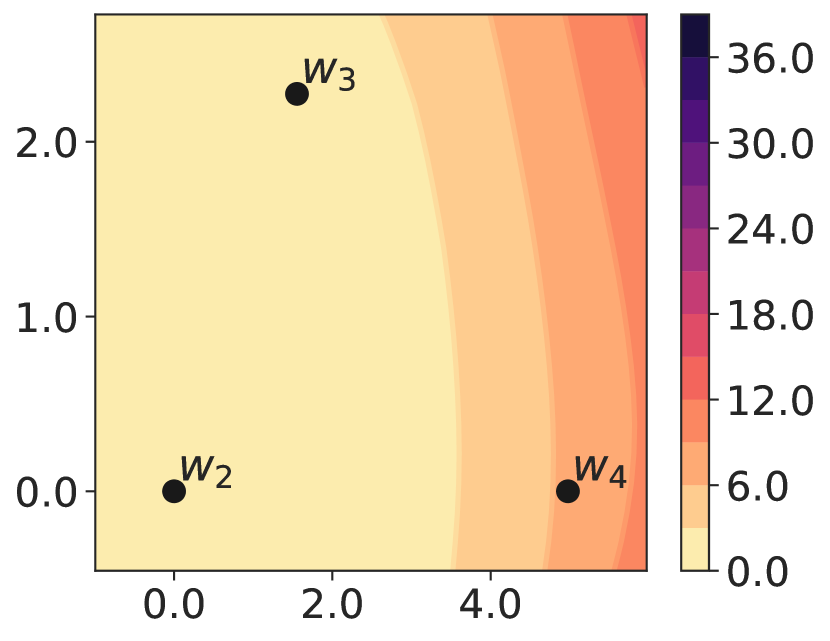
(h) ER w/ SAM (T2)

Figure 8: Loss contours for SVHN (T1) and MNIST (T2) of 5-dataset-CV. The top row visualizes loss contours for SVHN where w₁, w₂, and w₃ are minima obtained after sequential training on SVHN, MNIST, and nonMNIST, respectively. Similarly, the bottom row visualizes loss contours for MNIST where w₂, w₃, and w₄ are minima obtained after sequential training on tasks MNIST, nonMNIST, and Fashion-MNIST. All of the above models start with random weights. SAM (FT w/ SAM, ER w/ SAM) leads to wide task minima compared to finetune (FT) and ER methods.

Data set	Method	$\epsilon=5\times 10^{-4}$		$\epsilon=10^{-3}$
		w/o PT	w/ PT	w/o PT	w/ PT
5-dataset-CV	FT	$2.1_{0.6}$	$0.1_{0.0}$	$5.7_{1.6}$	$0.2_{0.0}$
	FT w/ SAM	$0.7_{0.2}$	$0.1_{0.0}$	$1.8_{0.4}$	$0.3_{0.0}$
Split CIFAR-50	FT	$2.3_{0.7}$	$0.2_{0.1}$	$6.1_{1.5}$	$0.4_{0.1}$
	FT w/ SAM	$0.7_{0.1}$	$0.2_{0.0}$	$2.0_{0.3}$	$0.6_{0.0}$

Table 6: Average sharpness (lower is flatter) of minima across tasks in a 100-dimensional random subspace. SAM significantly decreases the sharpness metric in comparison to Finetune (FT) method in the case of randomly initialized models (w/o PT).

5.2 Analyzing the influence of pre-training task minima curvature on forgetting

In the prior sections, we demonstrate that pre-trained initializations alleviate forgetting in lifelong learning scenarios by guiding optimization towards flat minima in the loss basin for sequentially trained tasks. Furthermore, we show that explicitly optimizing for the flatness of the loss basin using the sharpness-aware minimization (SAM) procedure leads to an additional reduction in forgetting. It is important to note that our discussion so far has mainly focused on the flatness of the loss basin near the fine-tuned task minima. However, we now inquire about the impact of the loss basin’s flatness (or sharpness) near the pre-training task minima on forgetting during lifelong learning. Specifically, we actively push a pre-trained model toward a region with low (or high) curvature. While such a model would benefit from learning structure from pre-training data, it would reside in flat (or sharp) regions of the loss basin with respect to the pre-training task. The question we pose is—What role does the curvature of the pre-training task minima play in lifelong learning, particularly in relation to forgetting in the fine-tuned task?

Experimental design. To answer the above question, we conduct a controlled experiment with SVHN as our pre-training task and analyze the forgetting in MNIST (and its subsets) when learning homogeneous as well as diverse tasks in a sequence. We pre-train two separate models on SVHN, ensuring that one model converges to a flat minimum using the SAM procedure, while the other model converges to a sharper minimum using the Nudged-SGD procedure (NSGD; Jastrzębski et al. (2019)). It is important to ensure that both models exhibit comparable generalization performance on SVHN. Subsequently, we initialize these models and perform sequential training on four diverse task sequences, starting with MNIST as our fine-tuning task. The task sequences are as follows: MNIST $\rightarrow$ SVHN, MNIST $\rightarrow$ notMNIST, MNIST $\rightarrow$ Fashion-MNIST, and MNIST $\rightarrow$ CIFAR10. To create homogeneous tasks in the Split MNIST data set, we randomly select two digits for each task. Considering that MNIST comprises 10 digits, we then create a random sequence of five tasks. By utilizing different random seeds, we generate different tasks and consequently obtain a variety of task orderings. In total, we generate 25 distinct task sequences for the Split MNIST data set. By examining the degree of forgetting observed in the case of (Split) MNIST, we can gain insights into the influence of the flatness (or sharpness) of the pre-training task minimum on the subsequent forgetting phenomenon. To ensure the broad applicability of our findings, we further conduct experiments using MNIST as the pre-training task and SVHN as the initial task for fine-tuning over four diverse task sequences.

Nudged-SGD (NSGD). Jastrzębski et al. (2019) investigate the SGD dynamics in relation to the sharpest directions of the loss basin and demonstrate that although SGD updates align closely with these directions, they generally fail to minimize the loss when solely constrained to these directions. In order to enhance both the convergence speed and the generalization of the resulting model, Jastrzębski et al. (2019) introduces a variant of SGD, called Nudged-SGD (NSGD). NSGD aims to reduce the alignment between the SGD update direction and the sharpest directions. Specifically, NSGD is implemented as follows: instead of the standard SGD update $\Delta w(t)=-\eta\mathbf{g}(t)$, NSGD employs a reduced learning rate, $\eta^{\prime}=\gamma\eta$, along the top $K$ eigenvectors. Meanwhile, NSGD continues to follow the standard SGD update in other directions. By setting $\gamma<1.0$, NSGD diminishes the updates along the top $K$ eigenvectors. As a result, training speed improves while converging to sharper and better generalizing minima in comparison to vanilla SGD. In our experimental setup, we utilize a randomly initialized ResNet-18 model. Following Jastrzębski et al. (2019), we set the parameters $\gamma$ to 0.01 and $K$ to 20. Additionally, we employ 100 training examples to compute the top $K$ eigenvectors using pytorch-hessian-eigenthings (Golmant et al., 2018) for every 100 training updates. Lastly, we set tolerance (relative accuracy for eigenvalues) to $1e^{-5}$ for determining the convergence of the Lanczos algorithm.

To begin, we conduct supervised pre-training of ResNet18 models using two different optimization procedures: SAM and NSGD, with the SVHN data set. Utilizing SAM, we achieve a validation accuracy of $92.0(\pm 0.4)$ and a maximum eigenvalue $\lambda_{1}^{max}$ of $338.5(\pm 91.5)$ (averaged over five runs). On the other hand, employing NSGD yields a validation accuracy of $92.4(\pm 0.3)$ and a maximum eigenvalue $\lambda_{1}^{max}$ of $1416.8(\pm 411.2)$ (also averaged over five runs). It is evident from these results that the NSGD leads to convergence towards sharper minima (as indicated by higher $\lambda_{1}^{max}$ values) and better generalization (as reflected in higher accuracy) compared to SAM and vanilla SGD. With vanilla SGD, we obtain a validation accuracy of $91.5(\pm 0.6)$ and a maximum eigenvalue $\lambda_{1}^{max}$ of $1241.3(\pm 236.5)$. Consequently, we have successfully obtained pre-trained models with varying levels of flatness or sharpness concerning the pre-training SVHN task, achieved through the SAM (Init:Flat) and NSGD (Init:Sharp) procedures.

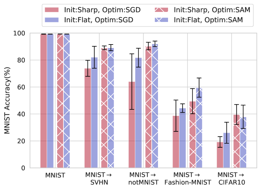
(a) MNIST Accuracy ($\uparrow$)

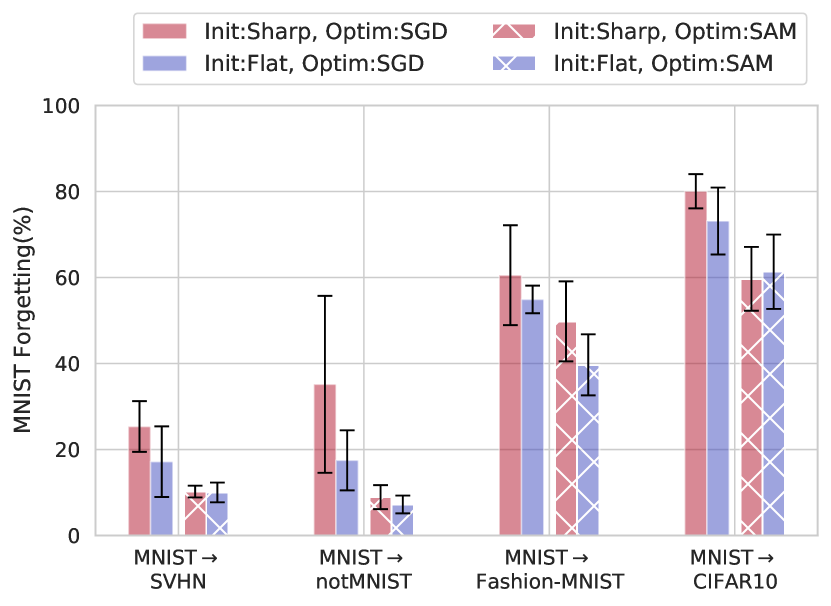
(b) MNIST Forgetting ($\downarrow$)

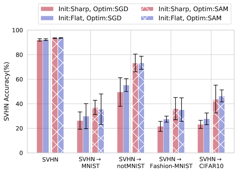
(c) SVHN Accuracy ($\uparrow$)

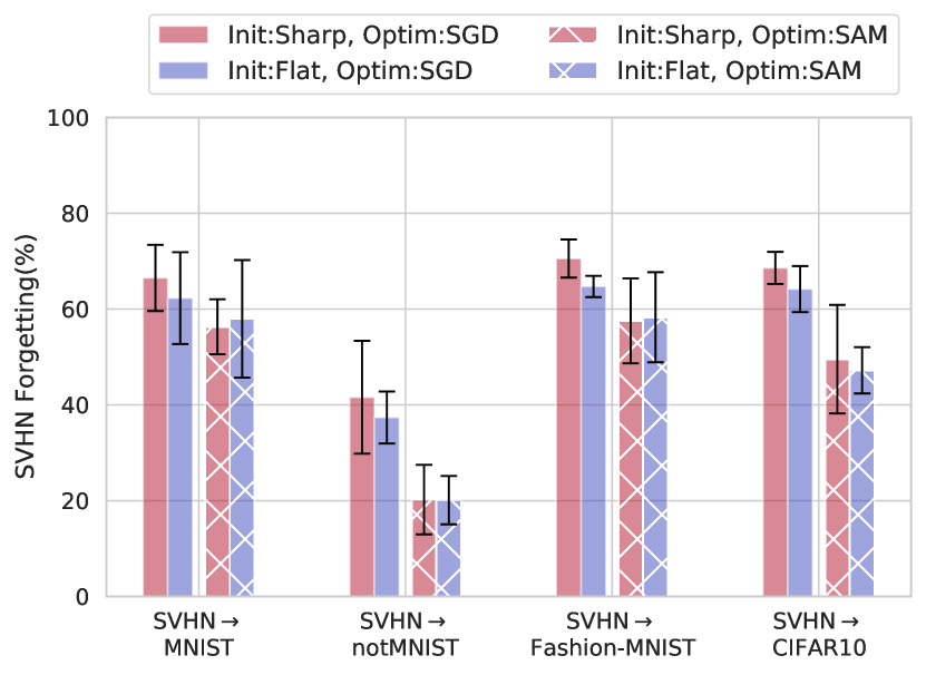
(d) SVHN Forgetting ($\downarrow$)

Figure 9: Comparing performance of the first task (MNIST in the top row, SVHN in the bottom row) after sequential training on the second task across different supervised pre-training initializations (Init:Sharp, Init:Flat) and optimization procedures (Optim:SGD, Optim:SAM). $\uparrow$ indicates higher performance, $\downarrow$ indicates lower performance. All metrics are averaged over 5 runs. Pre-trained models converged to flat minima with respect to the pre-training task (Init:Flat, Optim:SGD) exhibit reduced forgetting with SGD in comparison to sharp minima(Init:Sharp, Optim:SGD). Notably, explicitly promoting flatness (Optim:SAM) for the fine-tuning task yields an even greater reduction in forgetting.

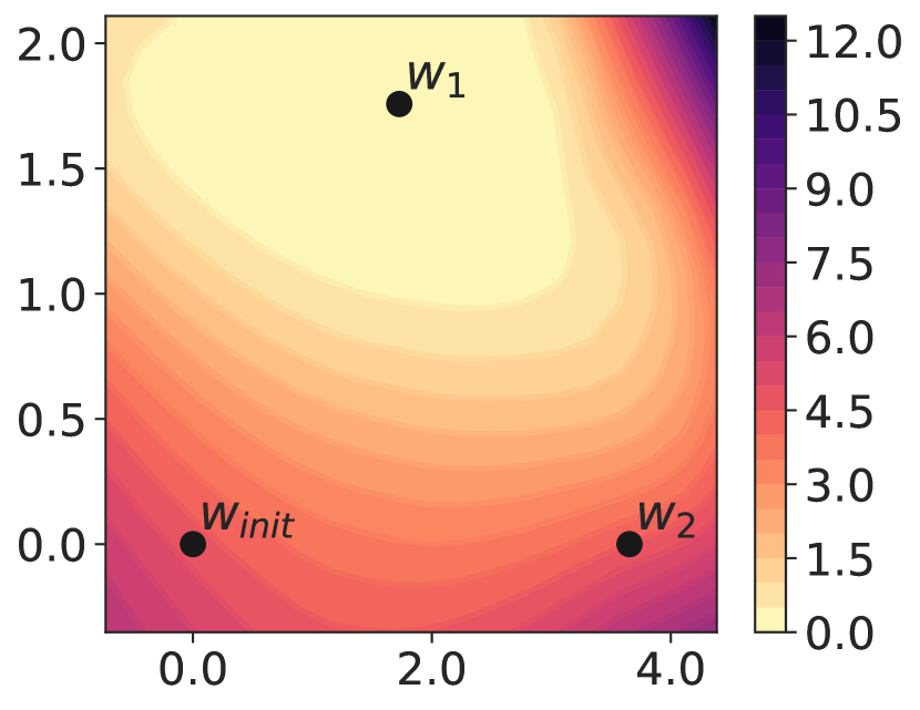
(a) Init:Sharp,
Optim:SGD

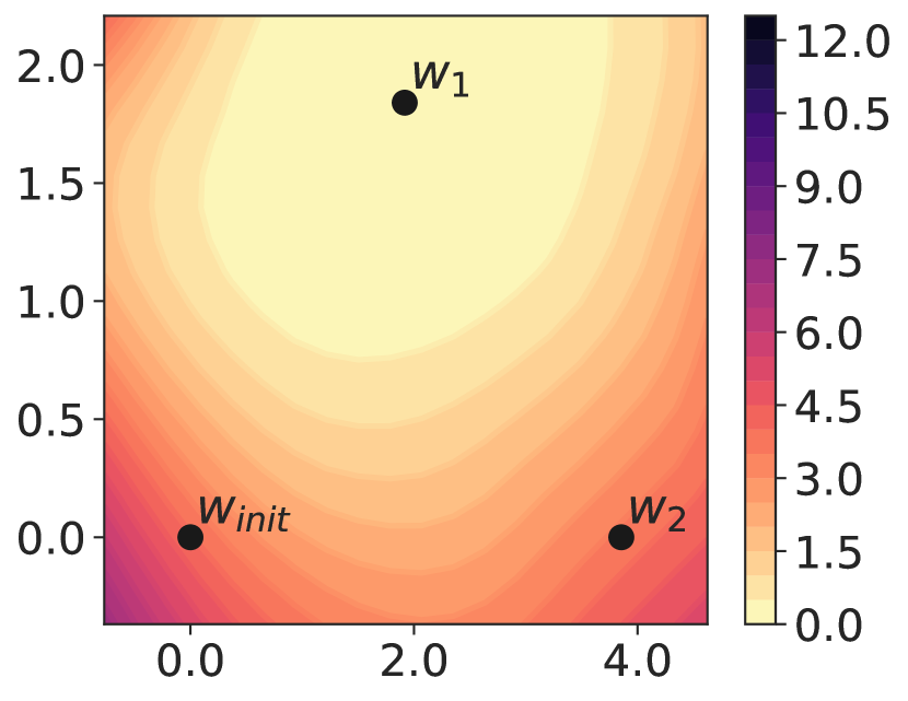
(b) Init:Flat,
Optim:SGD

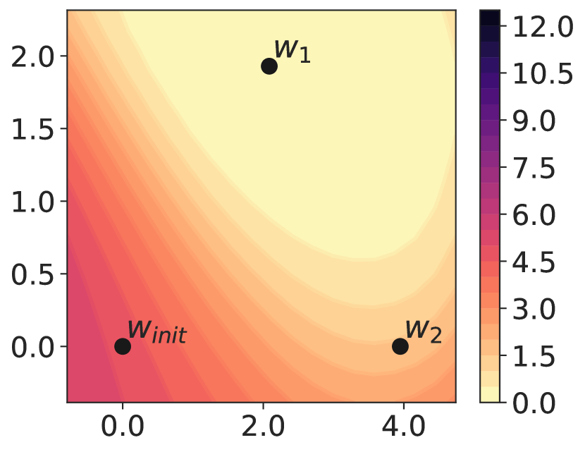
(c) Init:Sharp,
Optim:SAM

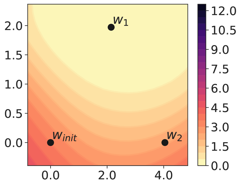
(d) Init:Flat,
Optim:SAM

Figure 10: Loss contours are shown for MNIST, with w${}_{\text{init}}$, w₁, and w₂ representing the minima obtained after supervised pre-training on SVHN, followed by sequential training on MNIST and nonMNIST, respectively. The models are initialized either with a sharp pre-trained model (Init:Sharp) or a flat pre-trained model (Init:Flat). (a), (b) starting with a flat pre-trained model results in a flatter loss basin for MNIST during sequential fine-tuning. (c), (d) explicitly optimizing for flat MNIST minima using SAM (Optim:SAM) leads to even wider task minima compared to vanilla SGD.

Discussion. In order to examine the influence of pre-training task minima curvature on forgetting during fine-tuning, we proceed to sequentially fine-tune the aforementioned pre-trained models (Init:Sharp or Init:Flat) on MNIST, followed by one of four tasks: SVHN, notMNIST, Fashion-MNIST, and CIFAR10. Additionally, to investigate the interplay between pre-trained minima curvature and optimization dynamics, we conduct sequential fine-tuning using either the vanilla SGD optimizer (Optim:SGD) or the SAM procedure (Optim:SAM). Figures 9(a) and 9(b) illustrate the accuracy and forgetting values for the MNIST task, respectively. From Figure 9(b), it is evident that when fine-tuning with vanilla SGD (Optim:SGD), pre-trained models with flat minima (Init:Flat; shown in blue) consistently exhibit lower levels of forgetting compared to models with sharp minima (Init:Sharp; shown in red) across various task sequences. However, the advantage provided by the flat pre-trained models appears to diminish when employing the SAM optimization procedure (see Init:Sharp, Optim:SAM and Init:Flat, Optim:SAM). This finding highlights that the flatness of the MNIST task minima plays a more significant role in reducing forgetting for MNIST compared to the initialization flatness with respect to the pre-training task (SVHN in this case) minima. Similar observations are reported in Figures 9(c) and 9(d) when MNIST is used as the pre-training task, and forgetting is analyzed for the SVHN task during continual learning.

In Figure 10, we provide a comparison of the loss contours for MNIST using sharp pre-trained initialization (Figure 10(a)) and flat pre-trained initialization (Figure 10(b)). Upon visual inspection, we observe that the flat pre-trained initialization results in a wider loss basin for the MNIST minima (w₁), thereby, explaining lesser forgetting of MNIST when continually training on notMNIST in the case of pre-trained initialized models (see Figure 9(b); Init:Flat, Optim:SGD). Furthermore, when SAM is applied, Optim:SAM (Figures 10(c), 10(d)) yields an even wider loss basin compared to Optim:SGD (Figures 10(a), 10(b)).

In Table 7, we present a comparison of average accuracy and forgetting on Split MNIST, focusing on sharp and flat supervised SVHN pre-trained initializations. Consistent with experiments involving diverse tasks (refer to Figure 9(b)), we find that Init:Flat, Optim:SGD ($4.3$) exhibits lower forgetting compared to Init:Sharp, Optim:SGD ($7.6$) in homogeneous tasks. This finding reinforces the notion that actively promoting flatness during pre-training, in addition to learning structure from abundant data, is beneficial for reducing forgetting in sequentially fine-tuned tasks. Moreover, initializing with a sharp pre-trained model and explicitly optimizing for flatness using SAM, as seen in Init:Sharp, Optim:SAM ($3.7$), yields an even greater reduction in forgetting compared to flat pre-trained initialization with vanilla SGD, i.e., Init:Flat, Optim:SGD ($4.3$), aligning with our previous observations (refer to Figure 9). However, we observe synergistic advantages when utilizing flat pre-trained models in conjunction with the SAM optimization procedure, resulting in minimal forgetting. Specifically, the combination of Init:Flat and Optim:SAM yields a forgetting value of $2.0$, showcasing the complementary benefits of these approaches.

To summarize, initiating fine-tuning with pre-trained models that have converged to flat minima with respect to the pre-training task helps mitigate forgetting. However, explicitly promoting flatness with respect to the fine-tuning task leads to a more pronounced reduction in forgetting.

	Optim:SGD			Optim:SAM
	Accuracy($\uparrow$)	Forgetting($\downarrow$)	LearnAcc($\uparrow$)	Accuracy($\uparrow$)	Forgetting($\downarrow$)	LearnAcc($\uparrow$)
Task-agnostic
Init:Random	$80.9_{9.7}$	$17.6_{9.0}$	$96.9_{5.9}$	$91.9_{5.3}$	$7.7_{5.2}$	$99.6_{0.3}$
Init:Meta	$89.5_{9.1}$	$9.8_{8.0}$	$98.8_{3.2}$	$\mathbf{92.3_{6.4}}$	$\mathbf{7.5_{6.3}}$	$99.6_{0.3}$
Supervised pre-training (SVHN)
Init:Sharp	$91.9_{8.1}$	$7.6_{7.6}$	$99.2_{1.8}$	$96.1_{4.7}$	$3.7_{4.6}$	$99.8_{0.2}$
Init:Flat	$95.2_{4.8}$	$4.3_{4.7}$	$99.1_{2.1}$	$\mathbf{97.8_{2.2}}$	$\mathbf{2.0_{2.1}}$	$99.7_{0.4}$

Table 7: Comparing the performance of Split MNIST in terms of average accuracy(%), forgetting(%), and learning accuracy(%), we analyze the impact of different initializations: random (Init:Random), task-agnostic meta-learned (Init:Meta), supervised pre-trained with explicit optimization for sharp minima (Init:Sharp), and supervised pre-trained with explicit optimization for flat minima (Init:Flat). We also consider different optimization approaches: vanilla SGD (Optim:SGD) and explicit optimization for flatness (Optim:SAM). $\uparrow$ indicates higher performance, while $\downarrow$ symbolizes lower performance. All metrics are averaged over 25 random task sequences. Our observations indicate that with Optim:SGD, MetaInit significantly reduces forgetting compared to random initialization, suggesting the benefits of initializing in flatter regions with minimal susceptibility to second-order effects. Also, pushing supervised pre-trained models towards flatter regions contributes to reduced forgetting. However, these gains diminish across all initialization schemes when explicitly optimizing for flatness (Optim:SAM) during lifelong learning. Nevertheless, we observe synergistic advantages when utilizing flat pre-trained or meta-initialized models in conjunction with the SAM procedure, resulting in minimal forgetting.

5.3 Analyzing the influence of task-agnostic favorable initializations on forgetting

Initialization is widely recognized as a crucial factor in a model’s learning dynamics and overall performance (Glorot and Bengio, 2010; LeCun et al., 2015; Mishkin and Matas, 2016). Various initialization schemes have been developed for specific network architectures, such as fully-connected networks (Pennington et al., 2017), residual networks (He et al., 2015), convolutional networks (Xiao et al., 2018), recurrent networks (Chen et al., 2018), and attention-based networks (Huang et al., 2020). However, these schemes are often architecture-specific and do not readily transfer to different or novel architectures. To overcome this limitation, Dauphin and Schoenholz (2019) propose MetaInit, an automated initialization search approach using task-agnostic meta-learning. On the other hand, pre-training has also been shown to yield favorable initializations in terms of optimization (Erhan et al., 2009; Hao et al., 2019; Neyshabur et al., 2020), making it a data-driven method for finding effective initialization schemes. In the previous sections, we observe that pre-trained initializations reduce forgetting during sequential fine-tuning. As these observations pertain to pre-trained initializations, this section aims to directly investigate the contribution of favorable initializations by removing the pre-training aspect. Specifically, we pose the question—Does good initializations from MetaInit, shown to facilitate gradient descent by starting in locally linear (or wider) regions with minimal second-order effects, also mitigate forgetting when compared to a random initialization in a sharper region?

Experimental Design. To address the above question, we perform controlled experiments to investigate the phenomenon of forgetting in the MNIST data set, both in the context of homogeneous and diverse task sequences. For this purpose, we employ the MetaInit algorithm (Dauphin and Schoenholz, 2019) to obtain a task-agnostic favorable initialization, which is independent of the specific task at hand. By comparing models initialized with the MetaInit approach to randomly initialized models, we aim to assess the impact of task-agnostic favorable initialization on forgetting. We examine the degree of forgetting specifically in the MNIST data set while sequentially learning four task sequences: MNIST $\rightarrow$ SVHN, MNIST $\rightarrow$ notMNIST, MNIST $\rightarrow$ Fashion-MNIST, and MNIST $\rightarrow$ CIFAR10, where MNIST serves as the initial task. Additionally, similar to the methodology described in Section 5.2, we conduct experiments involving homogeneous tasks from the Split MNIST data set.

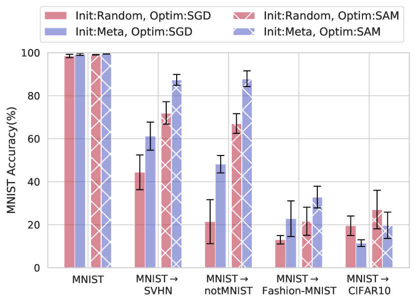
(a) MNIST Accuracy ($\uparrow$)

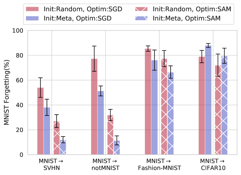
(b) MNIST Forgetting ($\downarrow$)

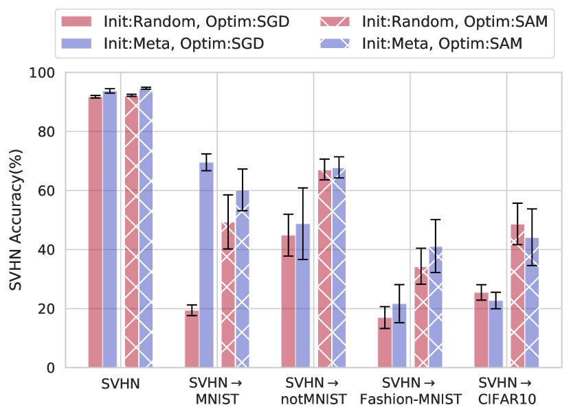
(c) SVHN Accuracy ($\uparrow$)

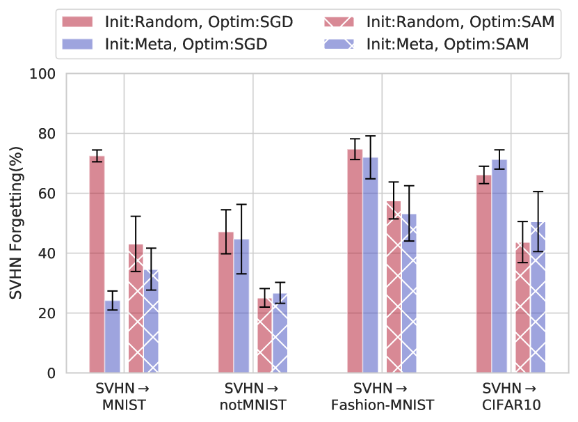
(d) SVHN Forgetting ($\downarrow$)

Figure 11: Comparing the performance of the first task (MNIST in the top row, SVHN in the bottom row) after sequential training on the second task, we examine the impact of random and task-agnostic MetaInit initialization strategy (Init:Random, Init:Meta) and optimization procedures (Optim:SGD, Optim:SAM). $\uparrow$ indicates higher performance, while $\downarrow$ symbolizes lower performance. All metrics are averaged over 5 runs. The results show that task-agnostic MetaInit models (Init:Meta, Optim:SGD) exhibit reduced forgetting with SGD compared to random initialization (Init:Random, Optim:SGD). Similarly to Figure 9, explicitly promoting flatness (Optim:SAM) for the sequential task leads to an even greater reduction in forgetting.

MetaInit. (Dauphin and Schoenholz, 2019) demonstrate that effective initializations exhibit characteristics that aid gradient descent by beginning in regions with minimal susceptibility to second-order effects. To quantify the impact of curvature (or second-order effects) around an initial choice of parameters, they introduce a quantity known as the gradient quotient (GQ). GQ measures the change in the gradient of a function following a single gradient descent step. Mathematically, the GQ is defined as follows

$$\text{GQ}(L,w)=\frac{1}{N}\left\|\frac{\mathbf{g}(w)-\mathbf{H}(w)\mathbf{g}(w)}{\mathbf{g}(w)+\epsilon}-1\right\|_{1}\approx\frac{1}{N}\left\|\frac{\mathbf{g}(w-\mathbf{g}(w))}{\mathbf{g}(w)+\epsilon}-1\right\|_{1},$$ (10)

where $w\in\mathbb{R}^{N}$ are network parameters, $L$ is an empirical loss computed over the batch of the examples, $\mathbf{g}(w)=\nabla L(w)$ is the gradient, $\mathbf{H}(w)=\nabla^{2}L(w)$ denotes Hessian matrix, $\epsilon=\epsilon_{0}(2_{\mathbf{g}(w)\geq 0}-1)$ with $\epsilon_{0}$ as a small constant and $||.||_{1}$ is the L1 vector norm. Alternatively, the GQ can be interpreted as the relative change in the gradient per parameter after a single step of gradient descent. As a result, parameters that cause a rapid change in the gradient exhibit large gradient quotients, while an optimal GQ of 0 is achieved when the loss function $L(w)$ behaves almost linearly, indicating a negligible Hessian matrix $\mathbf{H}(w)\approx 0$. Having established this metric to assess initialization quality, Dauphin and Schoenholz (2019) present MetaInit, a task-agnostic meta-learning algorithm aimed at obtaining a good initialization from suboptimal ones. The meta-objective of MetaInit is defined as follows

$$\text{MetaInit}(L,w^{*})=\arg\min_{w}\text{GQ}(L,w).$$ (11)

Following the methodology proposed by Dauphin and Schoenholz (2019), we optimize the aforementioned meta-objective using random input data ($\mathbf{x}\sim\mathcal{N}(0,1)$). It can be argued that solving for the meta-objective resembles a form of pre-training; however, no task-specific data is utilized in the learning process, thereby characterizing it as a task-agnostic initialization. Moreover, consistent with previous studies (Glorot and Bengio, 2010; Dauphin and Schoenholz, 2019), we solely adjust the norms of the initial weight matrices. We begin with five ResNet-18 models that are randomly initialized (Init:Random), with a GQ averaging $5476.2(\pm 2804.3)$. Through the MetaInit procedure (Init:Meta), we attain a final GQ value of $0.9(\pm 0.0)$.

Discussion. To investigate the impact of task-agnostic favorable initializations on forgetting, we sequentially train starting from the aforementioned initialization (Init:Random or Init:Meta) on MNIST, followed by one of four diverse tasks: SVHN, notMNIST, Fashion-MNIST, and CIFAR10. Furthermore, to explore the relationship between meta-learned initializations and optimization dynamics, we use either vanilla SGD (Optim:SGD) or the SAM procedure (Optim:SAM). The accuracy and forgetting values for the MNIST task are visualized in Figures 11(a) and 11(b), respectively. Figure 11(b) demonstrates that when optimized with vanilla SGD (Optim:SGD), meta-initialized models (Init:Meta; shown in blue) exhibit lower forgetting levels compared to randomly initialized models with high gradient quotient (Init:Random; shown in red) across various task sequences, except for CIFAR10, which differs significantly from MNIST. However, the advantage of meta-initialized models appears to diminish when employing the SAM optimization procedure (see Init:Random, Optim:SAM and Init:Meta, Optim:SAM), highlighting the more significant role of MNIST task minima flatness in reducing forgetting compared to the curvature of task-agnostic initialization. Similar observations are reported in Figures 11(c), 11(d) when starting from SVHN task followed by one of MNIST, notMNIST, Fashion-MNIST, and CIFAR10 task during lifelong learning.

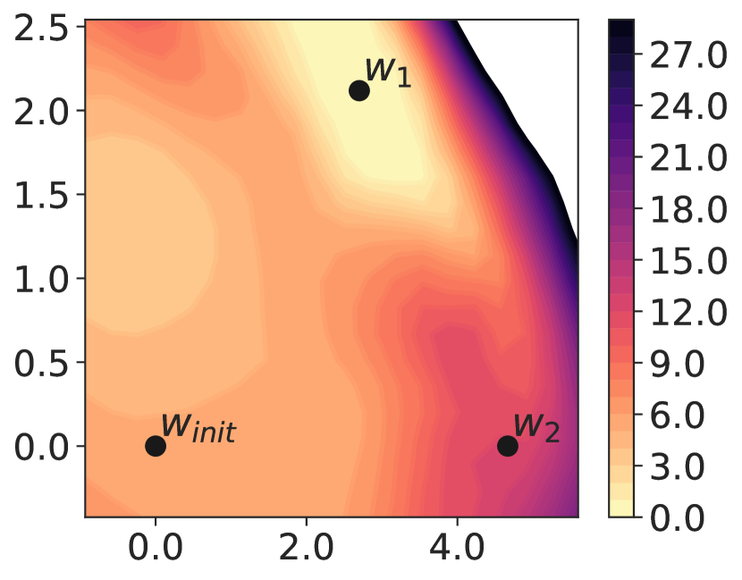
(a) Init:Random,
Optim:SGD

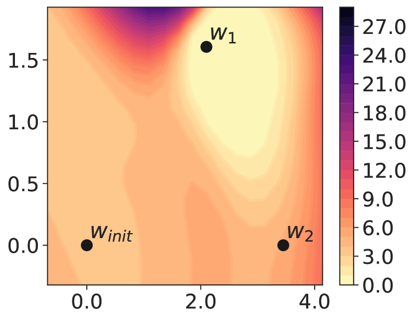
(b) Init:Meta,
Optim:SGD

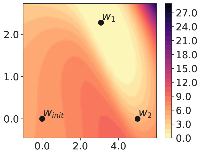
(c) Init:Random,
Optim:SAM

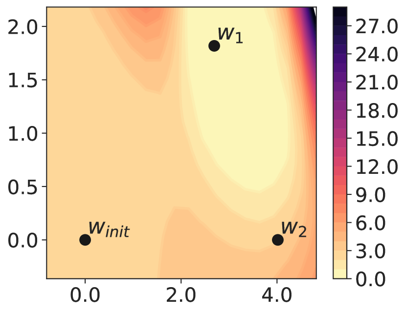
(d) Init:Meta,
Optim:SAM

Figure 12: Loss contours are shown for MNIST, with w${}_{\text{init}}$, w₁, and w₂ representing either random or task-agnostic initialization, followed by sequential training on MNIST and nonMNIST, respectively. The models are initialized either with a random strategy (Init:Random) or a MetaInit strategy (Init:Meta). (a), (b) starting with a MetaInit initialization results in a flatter loss basin for MNIST during sequential fine-tuning. (c), (d) explicitly optimizing for flat MNIST minima using SAM (Optim:SAM) leads to even wider task minima compared to vanilla SGD.

In Figure 12, we provide a comparison of the loss contours for MNIST using random initialization (Figure 12(a)) and task-agnostic MetaInit initialization (Figure 12(b)). Upon visual inspection, we observe that the MetaInit initialization results in a wider loss basin for the MNIST minima (w₁), thereby, explaining lesser forgetting of MNIST when continually training on notMNIST in the case of MetaInit initialized models (see Figure 11(b); Init:Meta, Optim:SGD). Furthermore, when SAM is applied, Optim:SAM (Figures 12(c), 12(d)) yields an even wider loss basin compared to Optim:SGD (Figures 12(a), 12(b)), explaining superior results with Optim:SAM (refer to Figures 11(a), 11(b)).

Table 7 presents a comparative analysis of average accuracy and forgetting on the Split MNIST data set, focusing on random initialization and task-agnostic MetaInit initialization. Consistent with our experiments involving diverse tasks (see Figure 11(b)), we observe that Init:Meta, Optim:SGD ($9.8$) exhibits significantly lower levels of forgetting compared to Init:Random, Optim:SGD ($17.6$) in the context of homogeneous tasks. This finding supports the notion that initializing model parameters with regions that are locally linear (or wider) and less affected by second-order effects can be advantageous for mitigating forgetting in lifelong learning. Furthermore, we find that random initialization and explicit optimization for flatness using SAM, as demonstrated by Init:Random, Optim:SAM ($7.7$), result in an even greater reduction in forgetting compared to MetaInit initialization with vanilla SGD, i.e., Init:Meta, Optim:SGD ($9.8$), which aligns with our previous observations (see Figure 11).

To summarize, initializing models with lower gradient quotients (achieved through task-agnostic meta-learning) in regions that are less susceptible to second-order effects help reduce forgetting during lifelong learning. However, the reduction in forgetting is more significant when explicitly promoting flatness in relation to the specific sequential learning task.

6 Related Work

In this section, we establish the connections to significant related works in the field.

Transfer learning from generic pre-trained models has sparked significant advancements in machine learning (Zhuang et al., 2021). Initially emerging in CV with the introduction of the ImageNet data set (Deng et al., 2009), the practice of transfer learning has also undergone its own “ImageNet revolution” in NLP. Notably, large models pre-trained on self-supervised tasks have exhibited remarkable performance across various language-related tasks (Peters et al., 2018; Howard and Ruder, 2018; Radford et al., 2018; Devlin et al., 2019; Liu et al., 2019; Raffel et al., 2020). The NIPS-95 workshop on “Learning to Learn” (Pan and Yang, 2009) initially motivated transfer learning as a means to facilitate lifelong learning. Our work revisits it in light of recent progress in transfer learning.

Lifelong learning approaches focus on the idea of mitigating the forgetting phenomenon and can be grouped into four categories: (1) regularization-based approaches either augment the loss function with extra penalty terms preventing important parameters learned on previous tasks from significantly deviating while training on the new task (Kirkpatrick et al., 2017; Zenke et al., 2017; Chaudhry et al., 2018a; Aljundi et al., 2018) and/ or enforce distillation-based penalty (Li and Hoiem, 2017; Dhar et al., 2019); (2) memory-based approaches that augment the model with episodic memory for sparse experience replay of previous task examples, either during training (Lopez-Paz and Ranzato, 2017; Chaudhry et al., 2018b, 2019; Guo et al., 2020) and/ or during inference (Rebuffi et al., 2017; de Masson d’Autume et al., 2019; Wang et al., 2020); some approaches learn generative model to simulate replay buffers (Shin et al., 2017; Sun et al., 2020); (3) optimization-based approaches that either maintain a space of gradient directions for previous tasks and projects the gradients of a new task in a direction orthogonal to that space, ensuring less disruption of older tasks (Farajtabar et al., 2020) or modify training regimes by specific hyperparameter configurations yielding wider minima and reducing the forgetting (Mirzadeh et al., 2020); and (4) architecture-based approaches that dynamically expand the network based upon new tasks (Rusu et al., 2016; Aljundi et al., 2017; Yoon et al., 2018; Sodhani et al., 2020), or iteratively learn mask (Mallya et al., 2018; Serra et al., 2018) or prunes networks (Mallya and Lazebnik, 2018) for new tasks. By formulation, these approaches do not undergo forgetting and hence we consider regularization and episodic memory-based approaches for our analysis.

Meta-learning involves the development of models capable of learning over time and has been employed in various studies focusing on lifelong learning (Riemer et al., 2019; Finn et al., 2019; Javed and White, 2019; Wang et al., 2020; Gupta et al., 2020). Notably, Caccia et al. (2020) propose a two-phase continual learning scenario, where the initial phase entails pre-training utilizing MAML (Finn et al., 2017), followed by continual deployment with task revisiting. They emphasize that deploying agents without any pre-training in lifelong learning scenarios would be impractical, a sentiment shared by other studies (Lomonaco et al., 2020). While some of these works employ pre-trained initializations, the comprehensive examination of the impact of pre-training in lifelong learning remains largely unexplored and is the focus of our work.

Optimization and loss landscape works have explored the relationship between pre-training and wider optima in single-task generalization (Hao et al., 2019; Neyshabur et al., 2020), as well as the effects of larger batch sizes on sharper minima and poorer generalization in single-task learning (Keskar et al., 2017). Additionally, Mirzadeh et al. (2021) compare minima resulting from multitask learning and continual learning, establishing that minima from continual learning are linearly connected to optimal sequential multitask minima but not to each other, leading to forgetting. While these studies examine the connection between pre-training and flat minima in single-task scenarios or the relationship between flat minima and model generalization, we extend this research by investigating whether the benefits of pre-training persist during sequential training on multiple tasks. We explore the effects of pre-training on loss landscapes throughout lifelong learning and validate a hypothesis that elucidates the role of pre-training in lifelong learning.

7 Discussion

In this paper, we investigate the role of pre-training in lifelong learning, examining various benchmarks and modalities. Our findings reveal that models with pre-trained initializations exhibit significantly reduced forgetting compared to models with random initializations. Despite pre-trained models starting with higher task performance, they undergo lesser forgetting. This observation holds even when comparing a sequentially fine-tuned pre-trained model, without additional regularization to mitigate forgetting, to a randomly initialized model trained with state-of-the-art lifelong learning methods. A key insight is that lifelong learning methods should explore the learning of generic initializations for future tasks rather than solely focusing on alleviating the forgetting of previous tasks. Furthermore, our analysis relating to different pre-trained models indicates that while increased model capacity provides benefits up to a certain point, the quality of pre-trained representations becomes more crucial when considering longer and more diverse task sequences.

To explain the above phenomenon, we conduct several analyses of the loss landscapes throughout continual training for models initialized randomly and with pre-training. Our findings reveal that the minima attained by the pre-trained models after each task exhibit significantly flatter characteristics compared to those obtained by randomly initialized models. Consequently, even if pre-trained models deviate from the original flat task minima, the task loss does not experience a significant increase, thereby undergoing less forgetting. Furthermore, explicitly seeking flat basins using the SAM procedure yields even lower forgetting than existing methods. Integrating SAM into the baselines surpasses state-of-the-art techniques, underscoring its valuable contribution to advancing lifelong learning methods. Lastly, our analysis of various initializations, including task-agnostic meta-learned and supervised pre-trained models explicitly guided towards flat loss regions, showcases the synergistic behavior that arises when combined with the SAM procedure during sequential fine-tuning.

Acknowledgments and Disclosure of Funding

We thank the anonymous reviewers and Action Editor for their valuable feedback and suggestions, which helped improve the paper. We also thank Janarthanan Rajendran, Sai Krishna Rallabandi, Khyathi Raghavi Chandu, Saujas Vaduguru, and Divyansh Kaushik for reviewing the paper and providing valuable comments. We are also grateful to Mojtaba Faramarzi for helping with ImageNet and CIFAR-100 class hierarchies, and to Hadi Nekoei, and Paul-Aymeric McRae for reviewing our code. We like to acknowledge CMU Workhorse, TIR group, and Compute Canada for providing compute resources for this work. This project is funded in part by DSO National Laboratories. Sarath Chandar is supported by a Canada CIFAR AI Chair and an NSERC Discovery Grant.

Appendix A Implementation Details

A.1 CV Experiments

For all vision experiments, we use the full ResNet-18 He et al. (2016) architecture, with the final linear layer replaced (the number of outputs corresponds to the total number of classes in all given tasks). During inference, only the subset of outputs corresponding to the given task is considered. In accordance with (He et al., 2015), for random initialization strategy, we initialize weight tensors using the Kaiming normal distribution, while setting batch normalization weights to 1 and biases to 0. All images are resized to $224\times 224$, and normalized with $\mu=(0.485,0.456,0.406)$ and $\sigma=(0.229,0.224,0.225)$. We used an SGD optimizer with the learning rate set to $.01$ for all methods (we did a hyperparameter search for both pre-trained and randomly initialized models and found the learning rate $0.01$ resulted in a good learning accuracy for both pre-trained and randomly initialized models). The batch size was set to $10$ for the Split CIFAR-50 and Split CIFAR-100 experiments and $64$ for the 5-dataset-CV experiments. The memory per class for ER was set to 1, and the $\lambda$ parameter for EWC was also set to 1. For Stable SGD, we performed a hyperparameter sweep over the parameters specified in the original paper, namely:

• initial learning rate: [.25 (Split CIFAR-100-R, Split CIFAR-50-R, 5-dataset-CV-R), .1, .01 (Split CIFAR-100-PT, Split CIFAR-50-PT), .001 (5-dataset-CV-PT)]

• learning rate decay: [0.9 (Split CIFAR-50-R, 5-dataset-CV-R, Split CIFAR-100-PT), 0.85 (Split CIFAR-100-R, Split CIFAR-50-PT), 0.8 (5-dataset-CV-PT)]

• batch size: [10 (all), 64]

• dropout: [0.5 (5-dataset-R), 0.25 (Split CIFAR-100-R, Split CIFAR-50-R, Split CIFAR-100-PT, Split CIFAR-50-PT, 5-dataset-CV-PT)]

For Mode Connectivity SGD, we adopted the hyperparameters specified in the original paper by Mirzadeh et al. (2021). To achieve continual learning minima, in experiments starting with the random initialization, we used an initial learning rate of 0.1, a learning rate decay of 0.8, a momentum of 0.8, a dropout of 0.1, a batch size of 10 for Split CIFAR-50 and Split CIFAR-100, and a batch size of 64 for the 5-dataset-CV. Conversely, in experiments starting with pre-trained initialization, we used an initial learning rate of 0.01, no learning rate decay, no momentum, no dropout, and a batch size of 64 for the 5-dataset-CV and 10 for Split CIFAR-10 and Split CIFAR-100. To obtain the linear mode connectivity minima, we employed 10 line samples, a learning rate of 0.01, a momentum of 0.8, a batch size of 64, a number of epochs set to 5, and initialized the position for the minima at 0.5.

A.2 NLP Experiments

For most of the text classification experiments, we use the Transformer architecture-based text encoder, DistilBERT-base (Sanh et al., 2019) to encode our input. In a single-sentence text classification task, $x_{t}$ is an input sentence to be classified. In a sentence-pair classification task, the concatenation of $x_{t}^{1}$ and $x_{t}^{2}$ sentences separated by a $[SEP]$ symbol is considered as an input $x_{t}$. DistilBERT produces a contextual representation of each token in $x_{t}$ including a special beginning of the sentence token symbol $[CLS]$. We use the representation of the $[CLS]$ symbol from the model as features for a linear task classifier. We have a separate classifier for each task. We mainly set hyper-parameters to default implementation from HuggingFace. For random initialization, we initialize weight tensors using the normal distribution $\mathcal{N}\sim(0,0.02)$, biases to 0, layer normalization weights to 1 and biases to 0. We use Adam as our optimizer, set dropout $0.1$, the base learning rate to $2e^{-5}$, batch size to $32$, and the maximum total input sequence length after tokenization to $128$. For EWC, we set the regularization strength $\lambda$ to $100$ (as this ended up with comparable LA across other methods), and for ER, following (Chaudhry et al., 2019), the memory per class per task is set to $1$. For SAM, we set $\rho=0.02$ for all models (random as well as pre-trained) on 5-dataset-NLP and 15-dataset-NLP. For SplitYahooQA we set $\rho=0.001$. For our experiments involving encoder-decoder architecture, we utilize the pre-trained T5-Small v1.1 checkpoint from HuggingFace. Since encoder-only models have a separate classification head, we also incorporate a separate classification head in the T5 decoder. We employ the Adam optimizer, with a dropout rate of 0.1. The base learning rate is set to $3e^{-4}$, the batch size is set to 32, and the maximum total input sequence length is set to 128. In the case of SAM, we set the hyperparameter $\rho$ to 0.05 for both the 5-dataset-NLP and 15-dataset-NLP experiments.

A.3 Sharpness metric

The matrix $A\in\mathbb{R}^{n\times p}$ used for projecting the parameters onto a subspace is randomly sampled and then normalized row-wise. Since this matrix is very large, the computation of the pseudo-inverse $A^{+}$ (required for calculating the bounds in Equation 3) is very memory intensive and unstable. Instead, we directly calculate $A^{+}w$ by finding the least squares solution to $Ab=w$. To find the maximum referenced in Equation 4, we use the L-BFGS-B algorithm. We set the maximum number of iterations for the algorithm to 10, and to speed up computation, we directly provide the gradients along with the loss to the algorithm, instead of using the default 2-point finite difference gradient estimation.

For ResNet-18 ($n=11M$), we set $p=100$. However, for DistilBERT ($n=66M$) when we set $p=100$, we notice extremely small values for the sharpness metric. With the increase in the number of parameters, $n$, we should ideally increase random subspace projection dimension $p$. Setting larger $p(>100)$ values for DistilBERT, however, leads to memory issues relating to allocating space for $A$ and computing the bounds (even with the more efficient method discussed above). So instead of evaluating the sharpness metric in a random manifold, we perform the maximization in the entire space $\mathbb{R}^{n}$ (basically setting $A=I_{n}$). According to Keskar et al. (2017), when $\epsilon$ is small enough and $A=I_{n}$, the sharpness metric in Equation 4 relates to the largest eigenvalue of $\nabla^{2}L(w)$.

Appendix B Task-specific results

In order to understand the evolution of task-specific performance during continuous training, we visualize the task-specific results in Figures 13 and 14. Specifically, we compare the performance of pre-trained and randomly initialized ResNet-18/ DistilBERT, for the first three tasks in a sequence, across five random task ordering, when evaluated on 5-dataset-CV/5-dataset-NLP (diverse tasks). In general, we see that both models start with approximately equal task accuracy (except for CIFAR-10), but pre-trained initialization leads to lesser forgetting than randomly initialized models (consistent with our observation in Figure 1 for Split YahooQA). Moreover, given the heterogeneous nature of the downstream tasks, we see that performance gains (in terms of forgetting) from pre-trained initialization vary across different tasks.

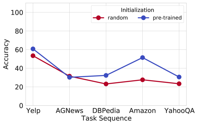
(a) Yelp (Seq1)

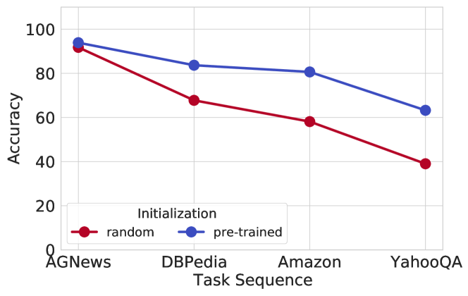
(b) AGNews (Seq1)

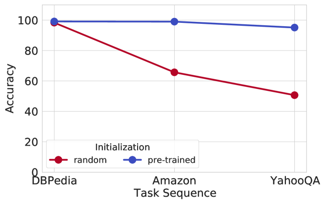
(c) DBPedia (Seq1)

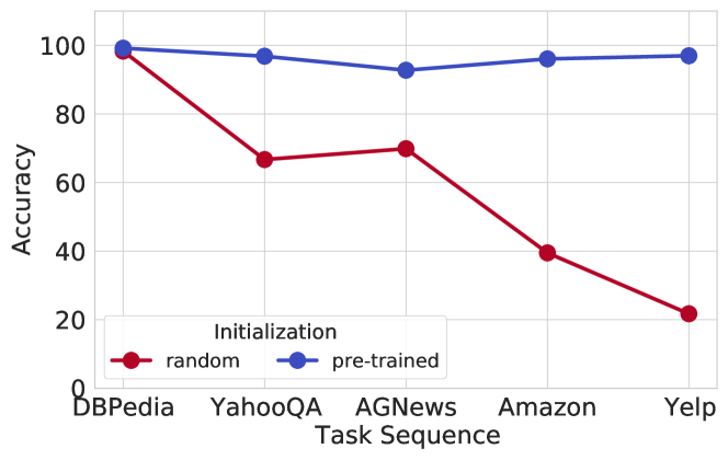
(d) DBPedia (Seq2)

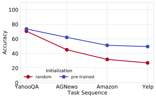
(e) YahooQA (Seq2)

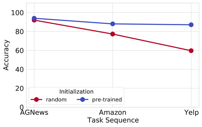
(f) AGNews (Seq2)

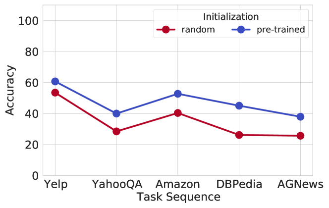
(g) Yelp (Seq3)

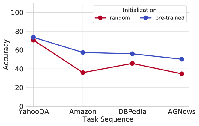
(h) YahooQA (Seq3)

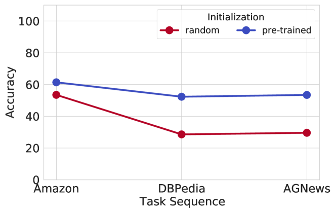
(i) Amazon (Seq3)

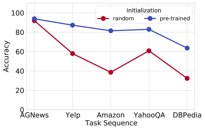
(j) AGNews (Seq4)

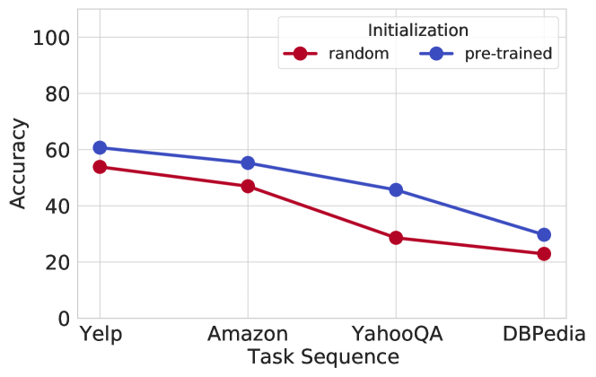
(k) Yelp (Seq4)

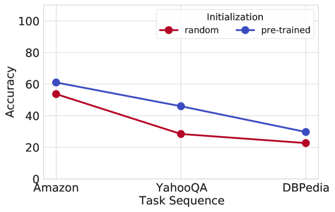
(l) Amazon (Seq4)

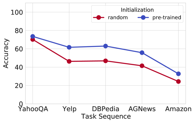
(m) YahooQA (Seq5)

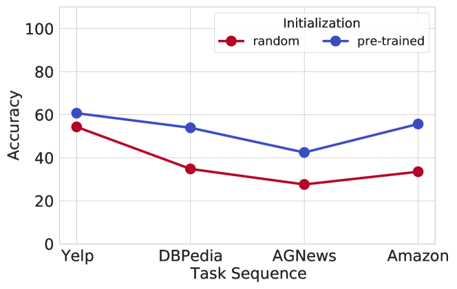
(n) Yelp (Seq5)

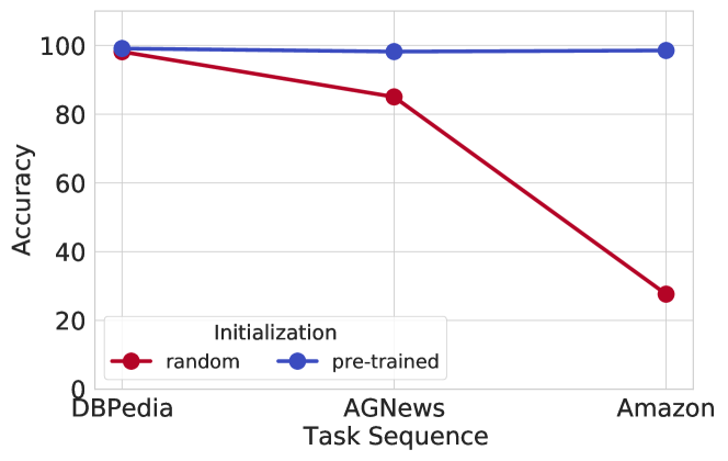
(o) DBPedia (Seq5)

Figure 13: Evolution of task accuracy during sequential training on 5-dataset-NLP. We compare the performance of pre-trained and randomly initialized models, for the first three tasks in a sequence, across five different random task orderings (Seq1, Seq2, Seq3, Seq4, Seq5). We see that both models start with approximately equal task accuracy, but pre-trained initialized models undergo lesser forgetting than randomly initialized models.

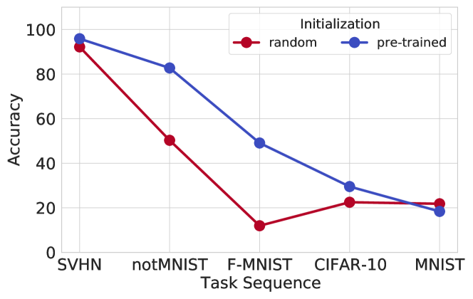
(a) SVHN (Seq1)

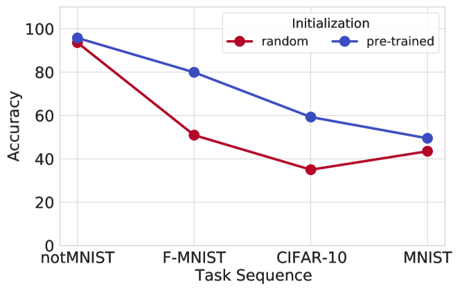
(b) notMNIST (Seq1)

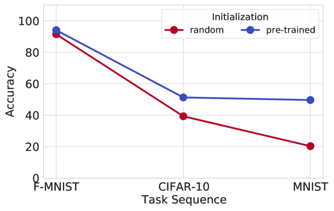
(c) Fashion-MNIST (Seq1)

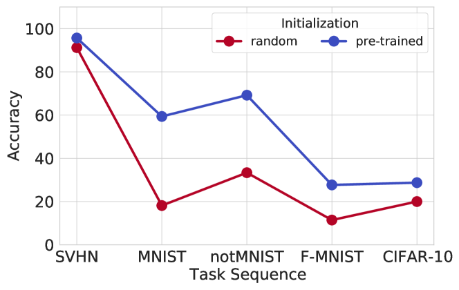
(d) SVHN (Seq2)

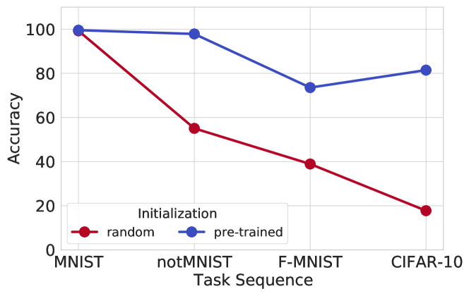
(e) MNIST (Seq2)

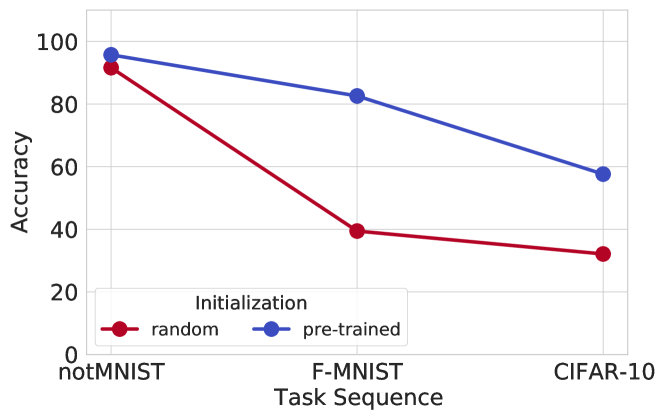
(f) notMNIST (Seq2)

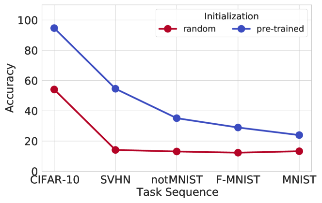
(g) CIFAR-10 (Seq3)

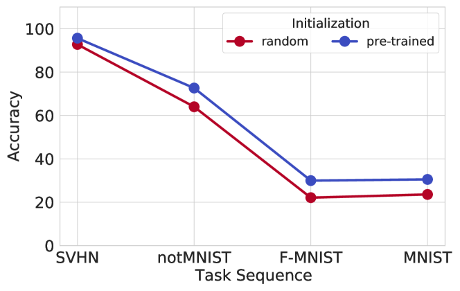
(h) SVHN (Seq3)

(i) notMNIST (Seq3)

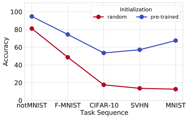
(j) notMNIST (Seq4)

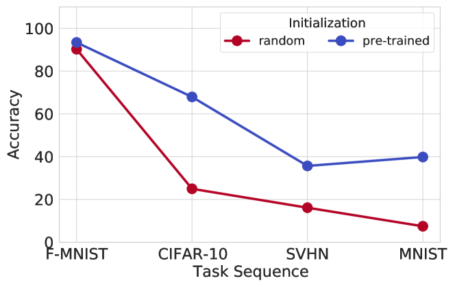
(k) Fashion-MNIST (Seq4)

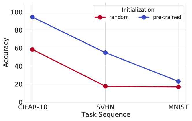
(l) CIFAR-10 (Seq4)

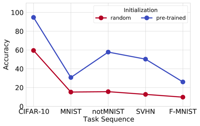
(m) CIFAR-10 (Seq5)

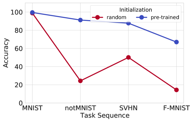
(n) MNIST (Seq5)

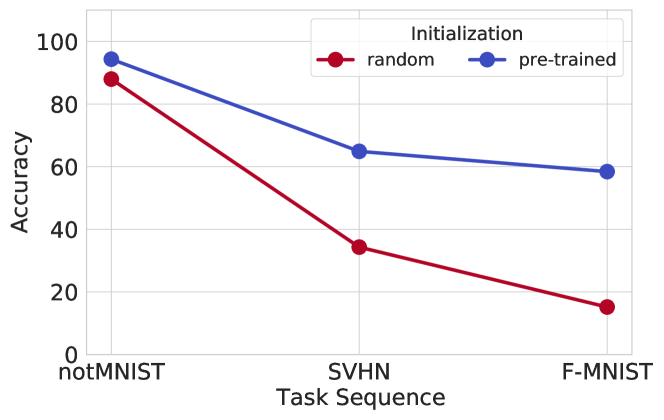
(o) notMNIST (Seq5)

Figure 14: Evolution of task accuracy during sequential training on 5-dataset-CV. We compare the performance of pre-trained and randomly initialized models, for the first three tasks in a sequence, across five different random task orderings (Seq1, Seq2, Seq3, Seq4, Seq5). We see that both models start with approximately equal task accuracy (except for CIFAR-10), but pre-trained initialized models undergo lesser forgetting than randomly initialized models.

B.1 5-dataset-NLP

For example, in the case of DBPedia (Figures 13(c), 13(d), 13(o)) and AGNews (Figures 13(b), 13(f), 13(j)) data sets, we see pre-trained DistilBERT undergoes little to almost no forgetting. One plausible explanation for these results is that both data sets are for the article classification tasks, DBPedia is Wikipedia article classification (14 classes) and AGNews is news article classification (4 classes), and share similar domains with the pre-training corpora (Wikipedia and Books). On the other hand, we see a significant forgetting in the case of Yelp (Figures 13(a), 13(g), 13(k)) and Amazon data sets (Figure 13(l)). Both of these data sets review sentiment classification tasks (5 classes). We know that the reviews domain (noisy text from Yelp.com and Amazon.com) is less similar to the pre-training corpora (clean text from Wikipedia and Books), and might be one of the reasons behind the drop in performance. Further, note that as we train on the sequence of tasks, we expect to see positive/ negative transfers from related/ unrelated tasks. For example, we see that the performance on Yelp improves significantly after training on Amazon (Figures 13(a), 13(g), 13(n)), demonstrating an example of positive transfer from the related task.

B.2 5-dataset-CV

Here, we report that the forgetting is more severe for SVHN (Figures 14(a), 14(d), 14(h)) and CIFAR-10 (Figures 14(g), 14(l), 14(m)) as compared to MNIST (Figures 14(e), 14(n)), notMNIST (Figures 14(b), 14(f), 14(i), 14(o)). Although SVHN and MNIST both are digit recognition tasks, we believe that the realistic nature (house numbers in Google Street View images) of SVHN images makes them more susceptible to forgetting, even in the case of pre-trained ResNet-18 models.

Appendix C Loss Landscape

C.1 Loss Contours

In this section, we present loss contours for task 1/ task 2 for all task sequences (refer to Section 2.3 for task sequences) for 5-dataset-NLP, Split YahooQA, Split CIFAR-50, and 5-dataset-CV. In line with our observation from the sharpness and linear model interpolation analyses, pre-trained initialized models lead to flatter task minima for subsequent tasks as well.

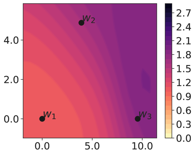
(a) Seq 1 (R)

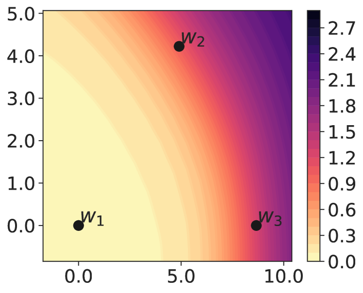
(b) Seq 2 (R)

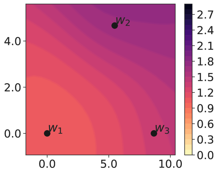
(c) Seq 3 (R)

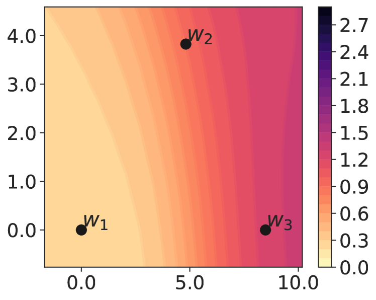
(d) Seq 4 (R)

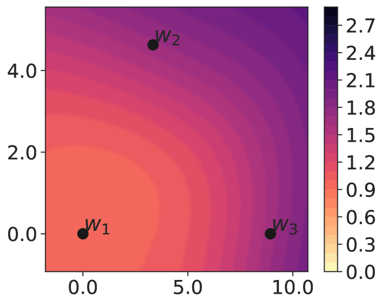
(e) Seq 5 (R)

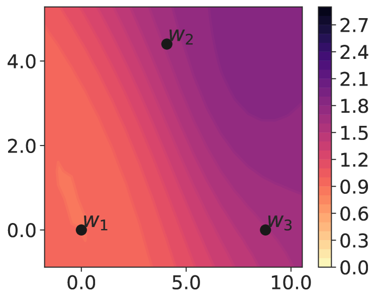
(f) Seq 1 (PT)

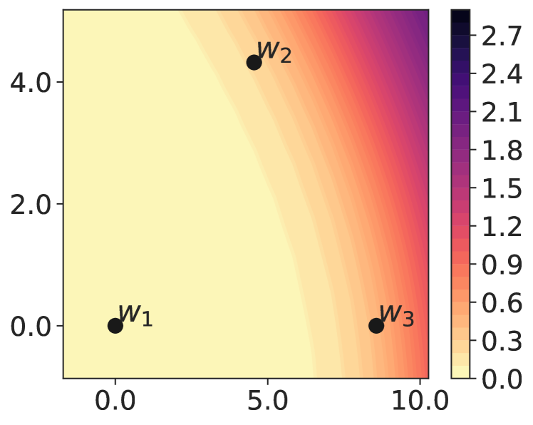
(g) Seq 2 (PT)

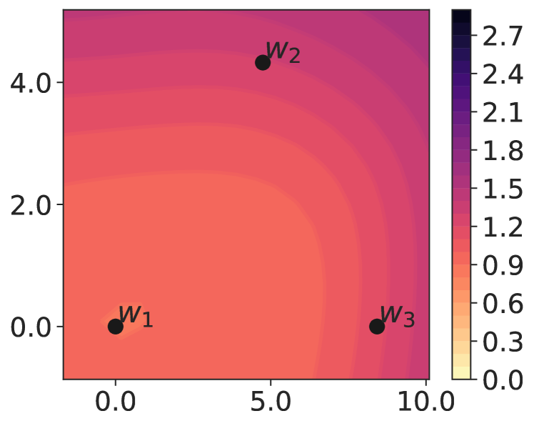
(h) Seq 3 (PT)

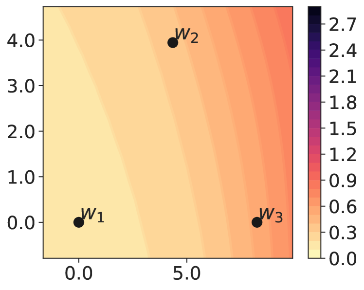
(i) Seq 4 (PT)

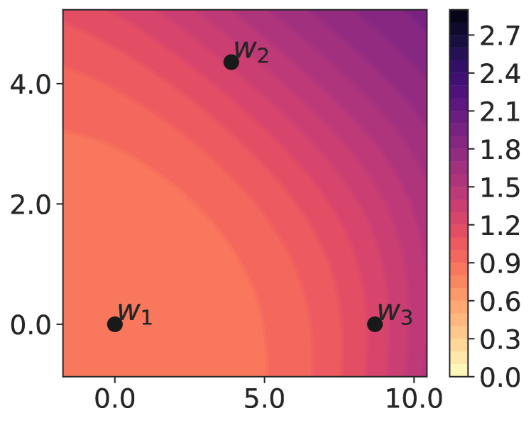
(j) Seq 5 (PT)

Figure 15: Loss contours for Task 1 on 5 task sequences of 5-dataset-NLP. Each contour shows the location of the model parameters after training sequentially on Task 1 (w₁), Task 2 (w₂), and Task 3 (w₃). The top row shows contours for randomly initialized models (R) and the bottom row shows contours for pre-trained initialized models (PT).

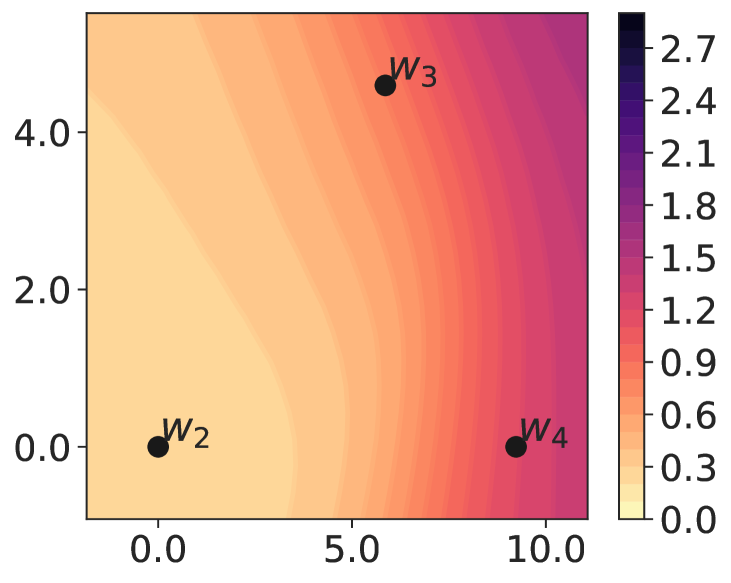
(a) Seq 1 (R)

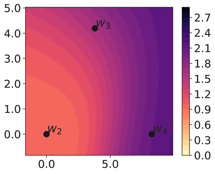
(b) Seq 2 (R)

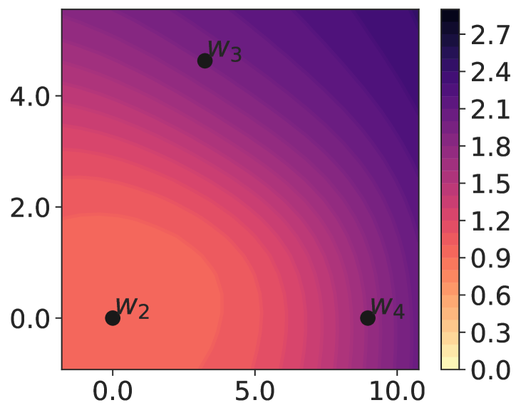
(c) Seq 3 (R)

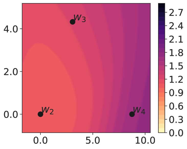
(d) Seq 4 (R)

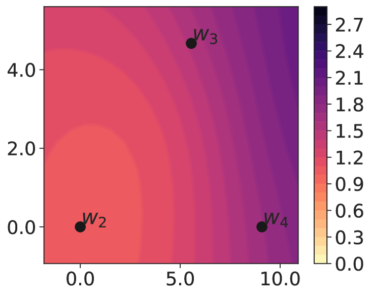
(e) Seq 5 (R)

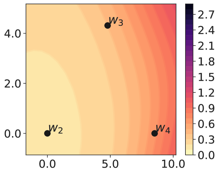
(f) Seq 1 (PT)

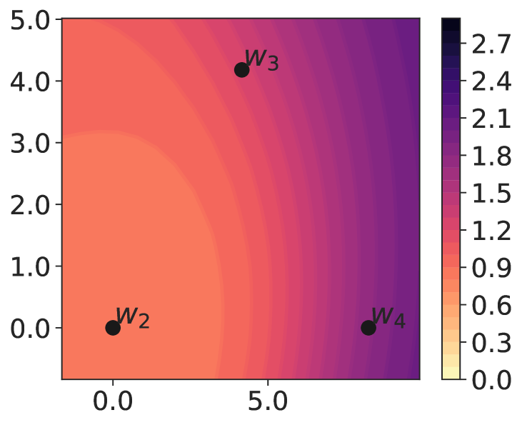
(g) Seq 2 (PT)

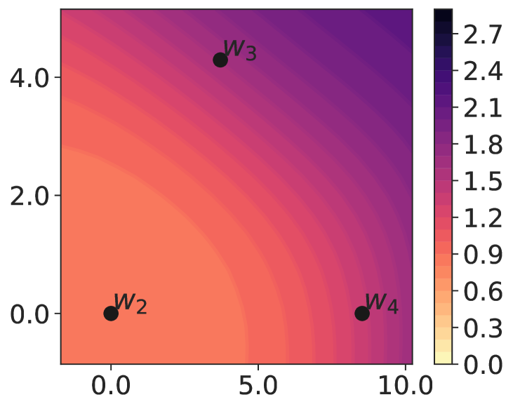
(h) Seq 3 (PT)

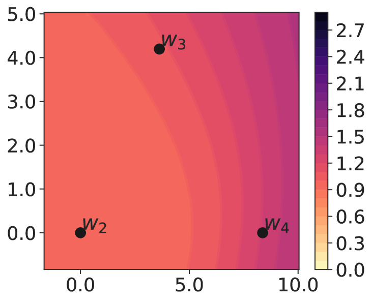
(i) Seq 4 (PT)

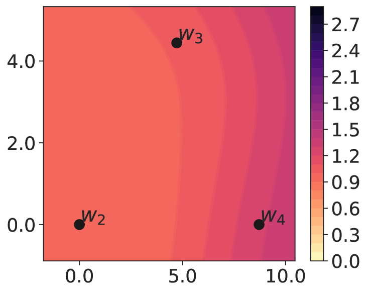
(j) Seq 5 (PT)

Figure 16: Loss contours for Task 2 on 5 task sequences of 5-dataset-NLP.

(a) Seq 1 (R)

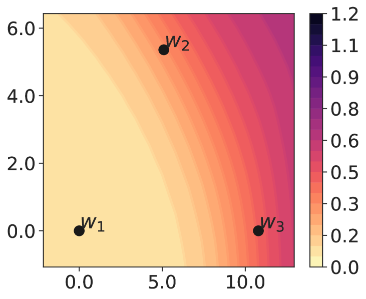
(b) Seq 2 (R)

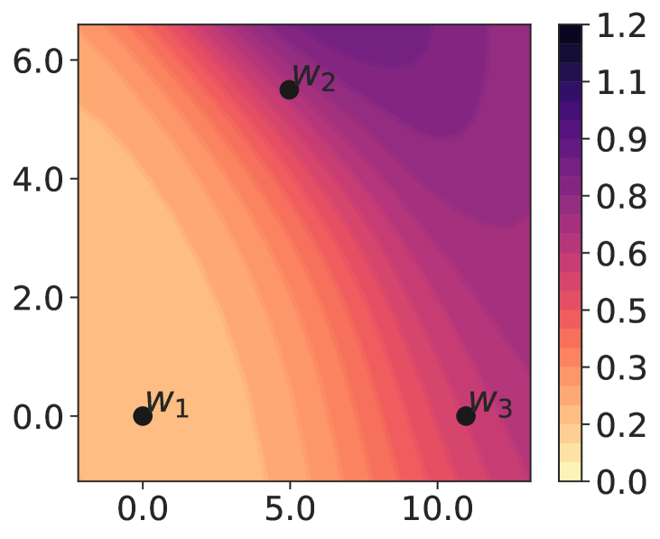
(c) Seq 3 (R)

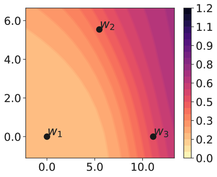
(d) Seq 4 (R)

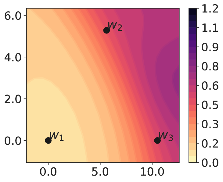
(e) Seq 5 (R)

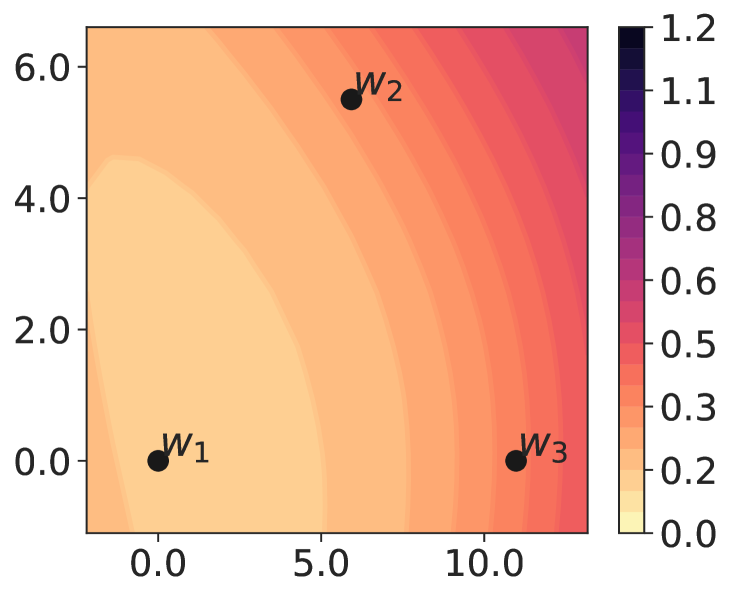
(f) Seq 1 (PT)

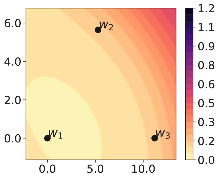
(g) Seq 2 (PT)

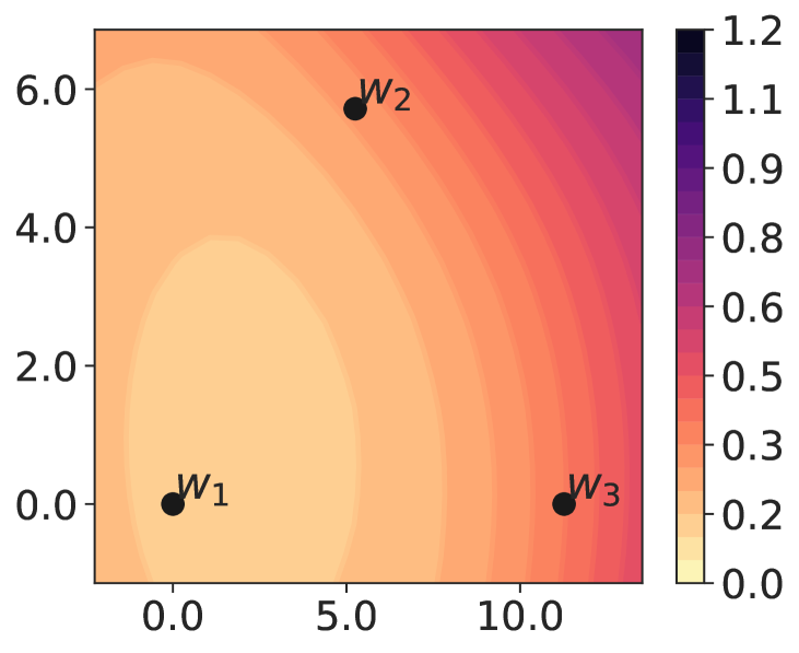
(h) Seq 3 (PT)

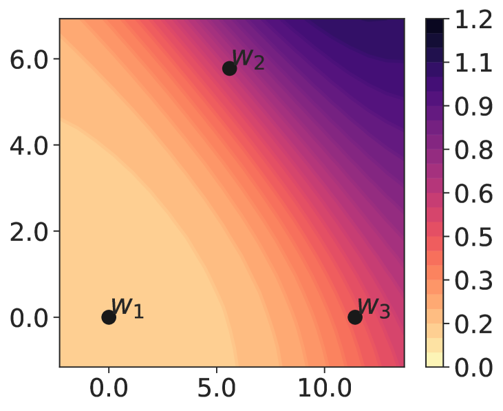
(i) Seq 4 (PT)

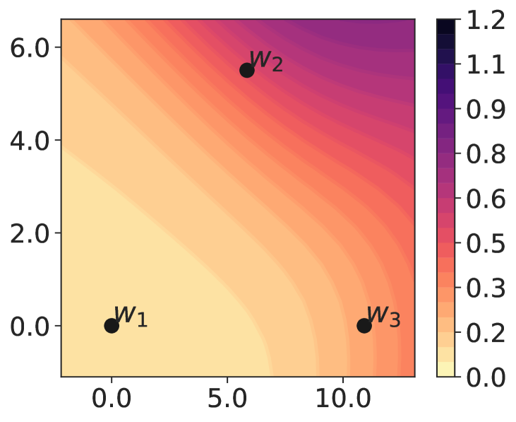
(j) Seq 5 (PT)

Figure 17: Loss contours for Task 1 on 5 task sequences of Split YahooQA.

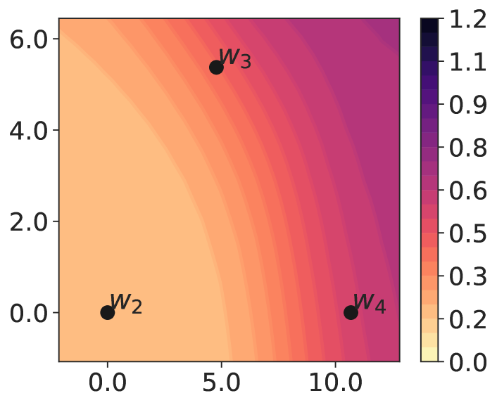
(a) Seq 1 (R)

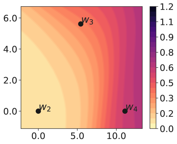
(b) Seq 2 (R)

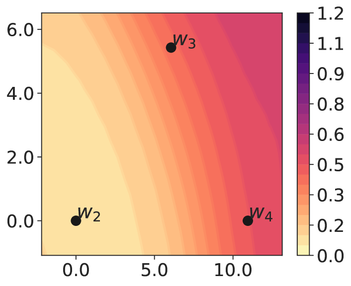
(c) Seq 3 (R)

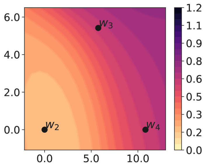
(d) Seq 4 (R)

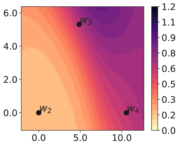
(e) Seq 5 (R)

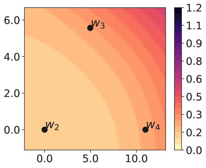
(f) Seq 1 (PT)

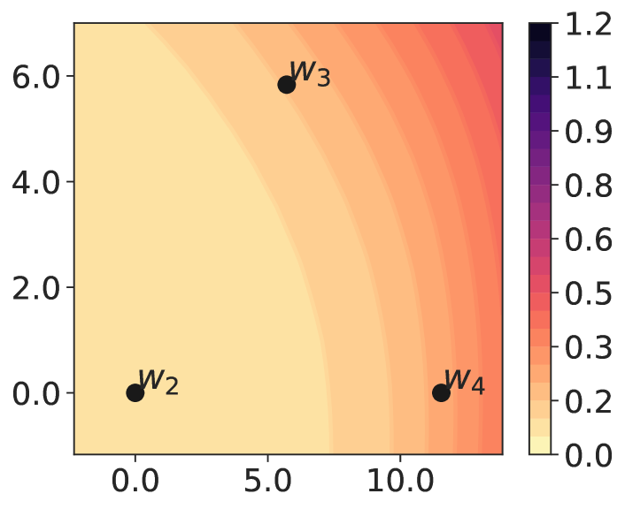
(g) Seq 2 (PT)

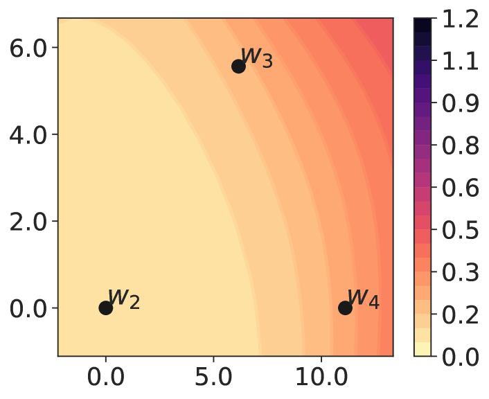
(h) Seq 3 (PT)

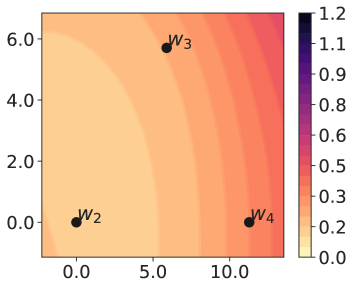
(i) Seq 4 (PT)

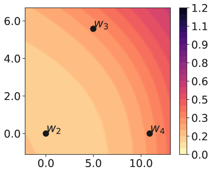
(j) Seq 5 (PT)

Figure 18: Loss contours for Task 2 on 5 task sequences of Split YahooQA.

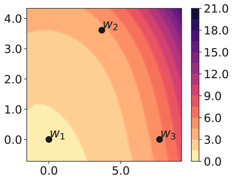
(a) Seq 1 (R)

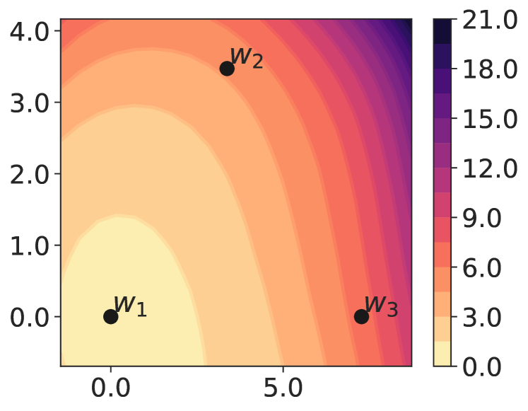
(b) Seq 2 (R)

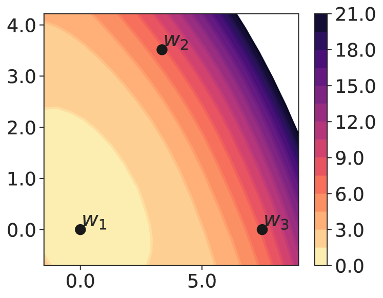
(c) Seq 3 (R)

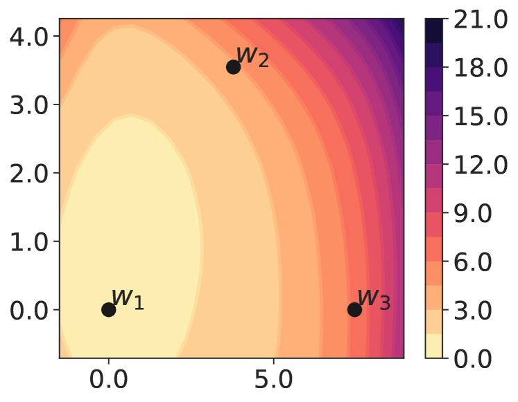
(d) Seq 4 (R)

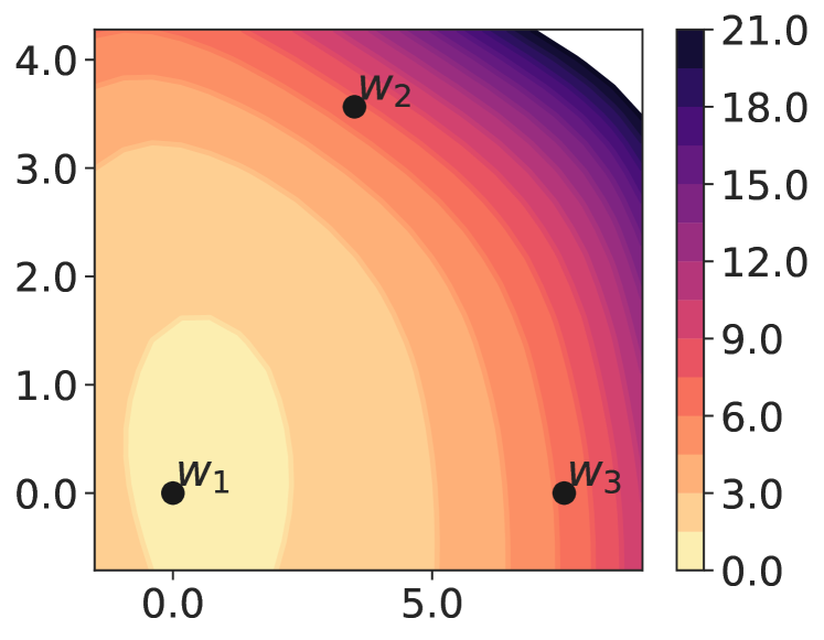
(e) Seq 5 (R)

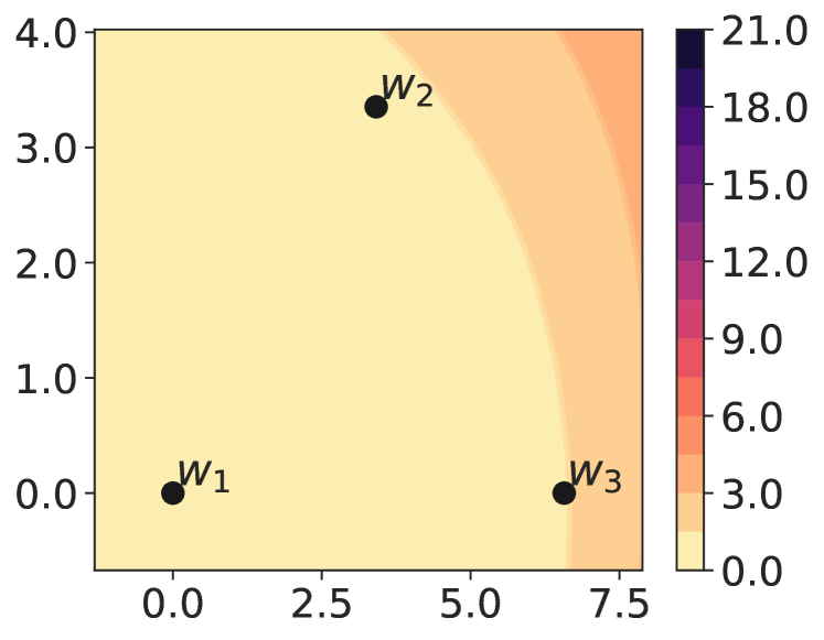
(f) Seq 1 (PT)

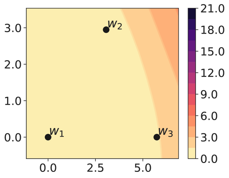
(g) Seq 2 (PT)

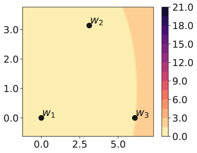
(h) Seq 3 (PT)

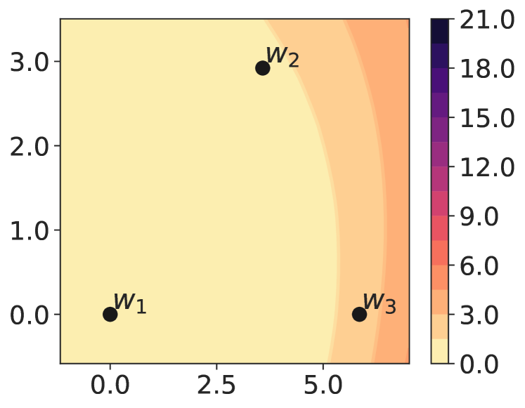
(i) Seq 4 (PT)

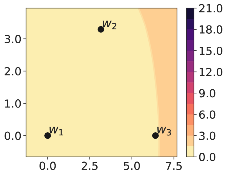
(j) Seq 5 (PT)

Figure 19: Loss contours for Task 1 on 5 task sequences of Split CIFAR-50.

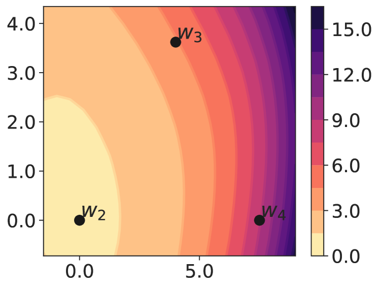
(a) Seq 1 (R)

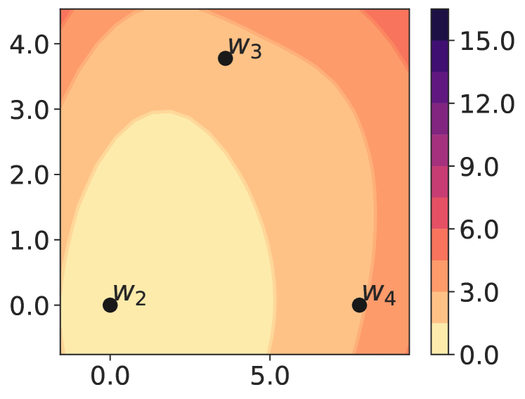
(b) Seq 2 (R)

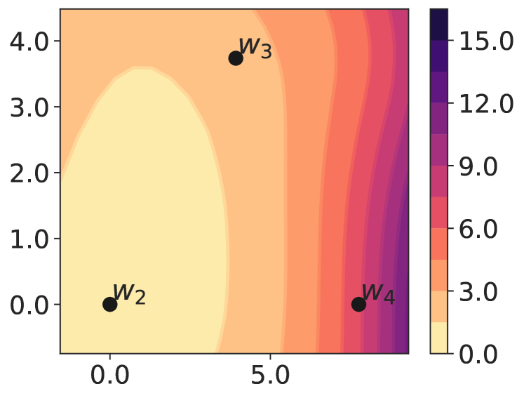
(c) Seq 3 (R)

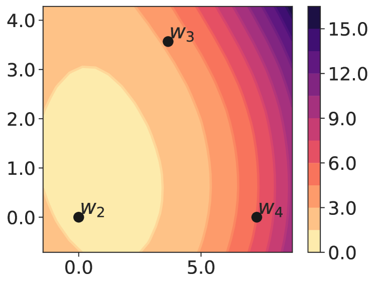
(d) Seq 4 (R)

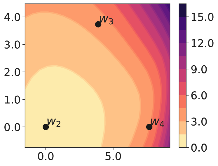
(e) Seq 5 (R)

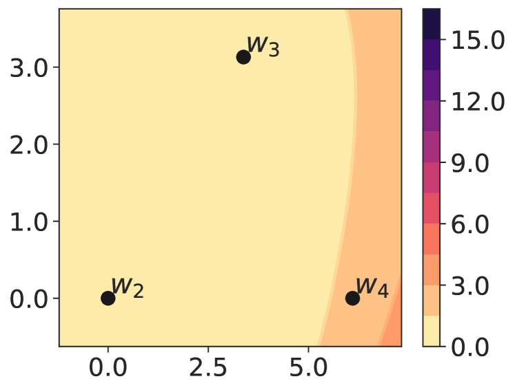
(f) Seq 1 (PT)

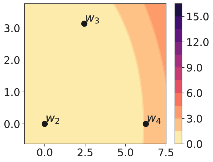
(g) Seq 2 (PT)

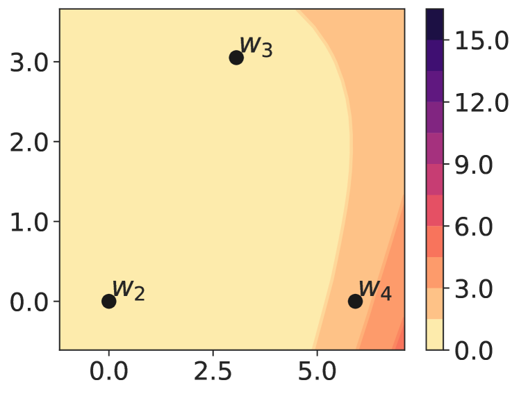
(h) Seq 3 (PT)

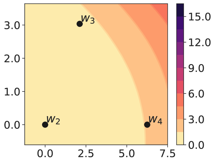
(i) Seq 4 (PT)

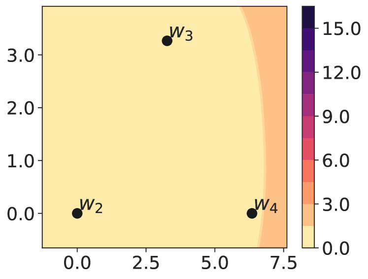
(j) Seq 5 (PT)

Figure 20: Loss contours for Task 2 on 5 task sequences of Split CIFAR-50.

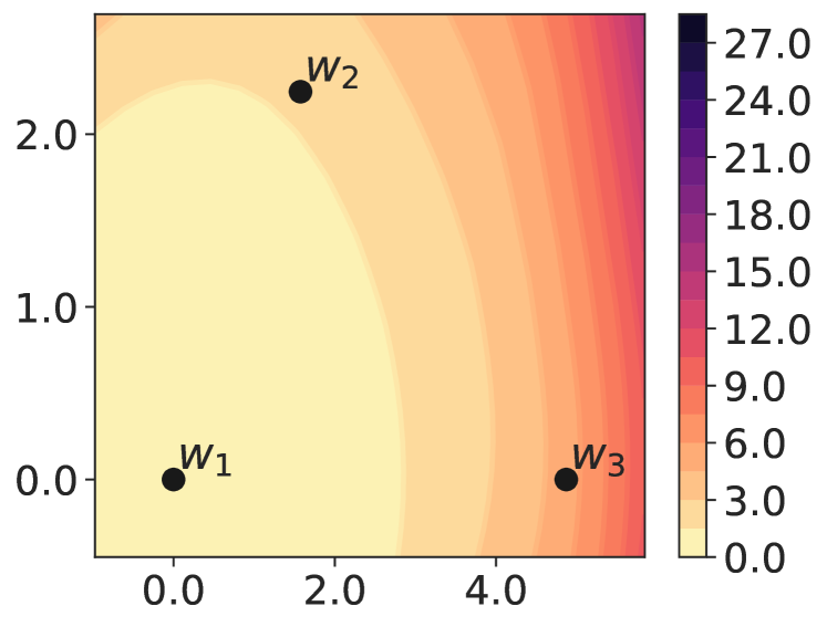
(a) Seq 1 (R)

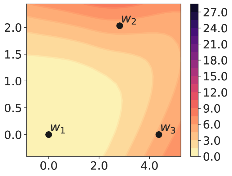
(b) Seq 2 (R)

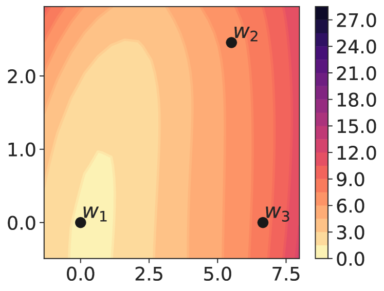
(c) Seq 3 (R)

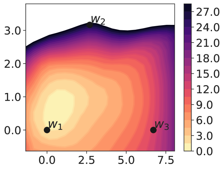
(d) Seq 4 (R)

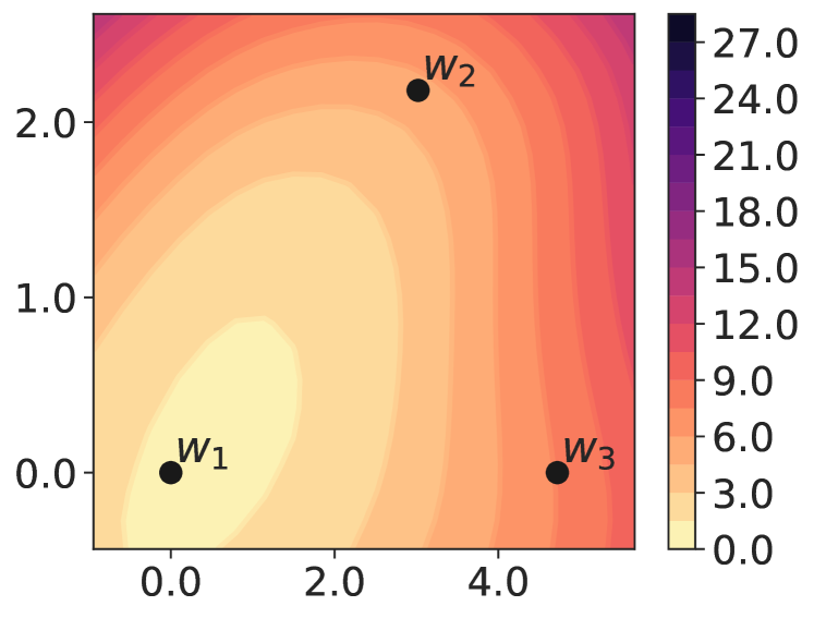
(e) Seq 5 (R)

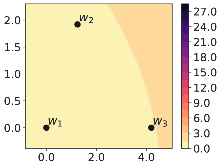
(f) Seq 1 (PT)

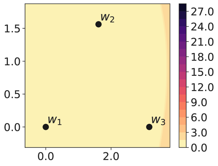
(g) Seq 2 (PT)

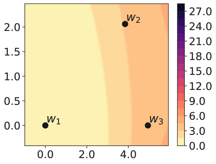
(h) Seq 3 (PT)

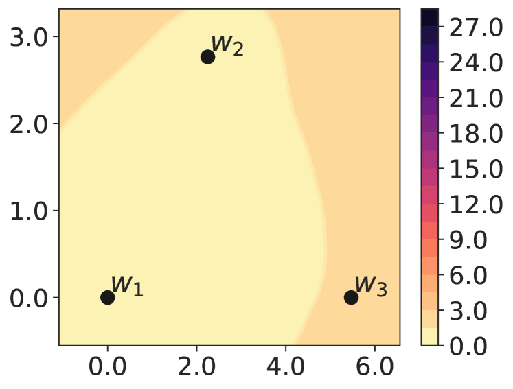
(i) Seq 4 (PT)

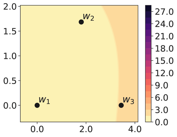
(j) Seq 5 (PT)

Figure 21: Loss contours for Task 1 on 5 task sequences of 5-dataset-CV.

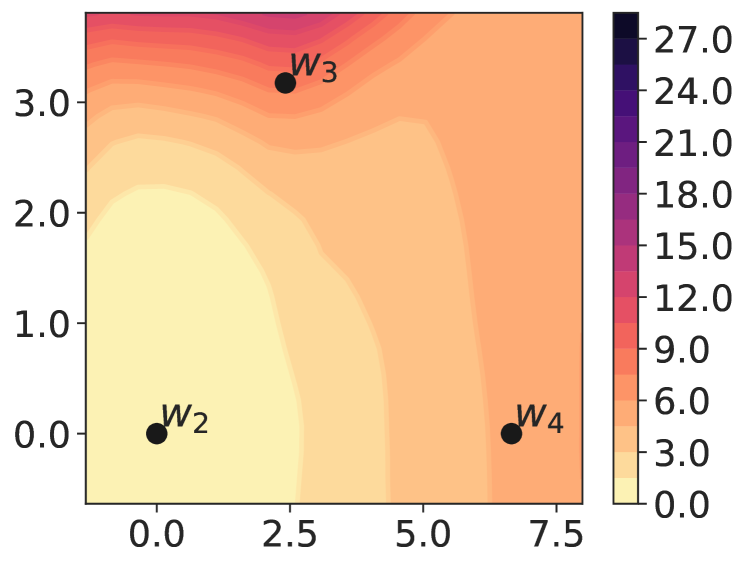
(a) Seq 1 (R)

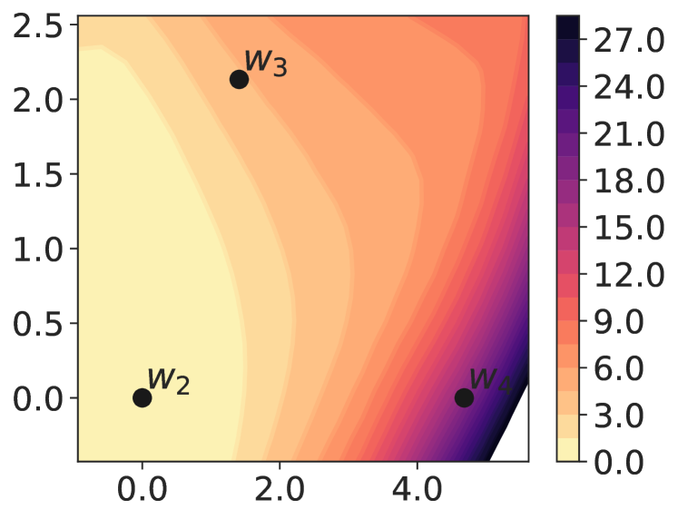
(b) Seq 2 (R)

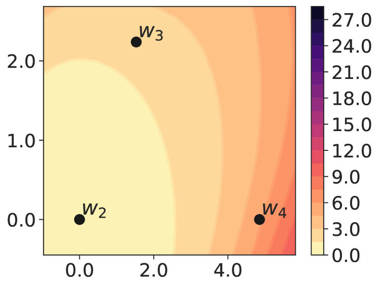
(c) Seq 3 (R)

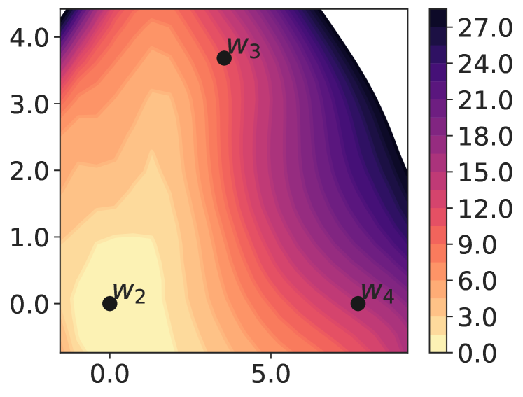
(d) Seq 4 (R)

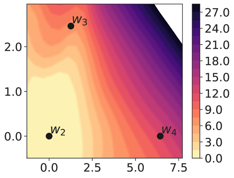
(e) Seq 5 (R)

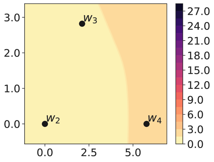
(f) Seq 1 (PT)

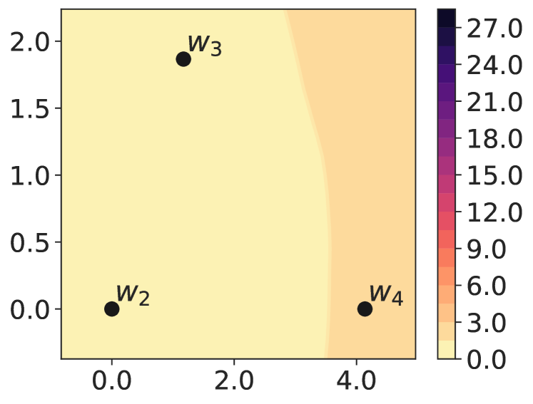
(g) Seq 2 (PT)

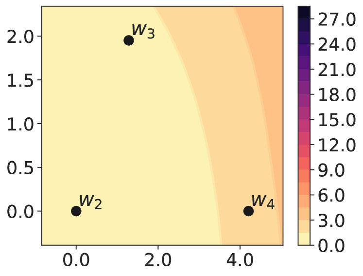
(h) Seq 3 (PT)

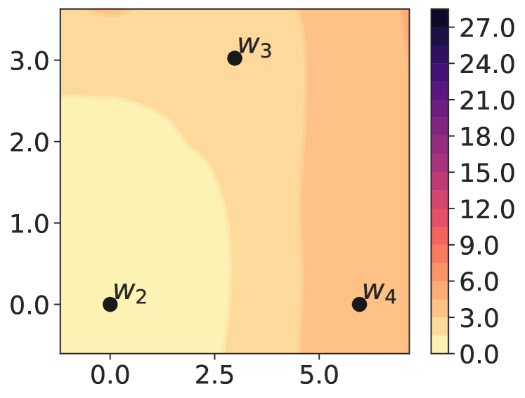
(i) Seq 4 (PT)

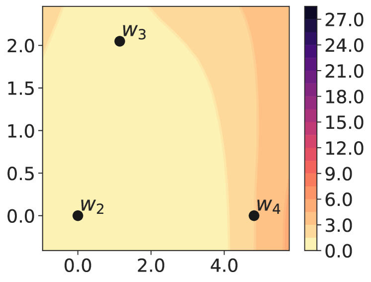
(j) Seq 5 (PT)

Figure 22: Loss contours for Task 2 on 5 task sequences of 5-dataset-CV.

References

- Abdelsalam et al. (2021) Mohamed Abdelsalam, Mojtaba Faramarzi, Shagun Sodhani, and Sarath Chandar. Iirc: Incremental implicitly-refined classification. In Proceedings of the IEEE/CVF Conference on Computer Vision and Pattern Recognition, pages 11038–11047, 2021.
- Aljundi et al. (2017) Rahaf Aljundi, Punarjay Chakravarty, and Tinne Tuytelaars. Expert gate: Lifelong learning with a network of experts. In Proceedings of the IEEE Conference on Computer Vision and Pattern Recognition, pages 3366–3375, 2017.
- Aljundi et al. (2018) Rahaf Aljundi, Francesca Babiloni, Mohamed Elhoseiny, Marcus Rohrbach, and Tinne Tuytelaars. Memory aware synapses: Learning what (not) to forget. In Proceedings of the European conference on computer vision (ECCV), pages 139–154, 2018.
- Bulatov (2011) Yaroslav Bulatov. Notmnist dataset. Technical report, Google (Books/OCR), 2011. URL http://yaroslavvb.blogspot.it/2011/09/notmnist-dataset.html.
- Caccia et al. (2020) Massimo Caccia, Pau Rodriguez, Oleksiy Ostapenko, Fabrice Normandin, Min Lin, Lucas Page-Caccia, Issam Hadj Laradji, Irina Rish, Alexandre Lacoste, David Vázquez, et al. Online fast adaptation and knowledge accumulation (osaka): a new approach to continual learning. Advances in Neural Information Processing Systems, 33:16532–16545, 2020.
- Chaudhry et al. (2018a) Arslan Chaudhry, Puneet K Dokania, Thalaiyasingam Ajanthan, and Philip HS Torr. Riemannian walk for incremental learning: Understanding forgetting and intransigence. In Proceedings of the European conference on computer vision (ECCV), pages 532–547, 2018a.
- Chaudhry et al. (2018b) Arslan Chaudhry, Marc’Aurelio Ranzato, Marcus Rohrbach, and Mohamed Elhoseiny. Efficient lifelong learning with a-gem. In International Conference on Learning Representations, 2018b.
- Chaudhry et al. (2019) Arslan Chaudhry, Marcus Rohrbach, Mohamed Elhoseiny, Thalaiyasingam Ajanthan, Puneet K Dokania, Philip HS Torr, and Marc’Aurelio Ranzato. On tiny episodic memories in continual learning. arXiv preprint arXiv:1902.10486, 2019.
- Chen et al. (2018) Minmin Chen, Jeffrey Pennington, and Samuel Schoenholz. Dynamical isometry and a mean field theory of rnns: Gating enables signal propagation in recurrent neural networks. In International Conference on Machine Learning, pages 873–882. PMLR, 2018.
- Chen and Liu (2018) Zhiyuan Chen and Bing Liu. Lifelong machine learning. Synthesis Lectures on Artificial Intelligence and Machine Learning, 12(3):1–207, 2018.
- Clark et al. (2019) Christopher Clark, Kenton Lee, Ming-Wei Chang, Tom Kwiatkowski, Michael Collins, and Kristina Toutanova. Boolq: Exploring the surprising difficulty of natural yes/no questions. In Proceedings of the 2019 Conference of the North American Chapter of the Association for Computational Linguistics: Human Language Technologies, Volume 1 (Long and Short Papers), pages 2924–2936, 2019.
- Dauphin and Schoenholz (2019) Yann N Dauphin and Samuel Schoenholz. Metainit: Initializing learning by learning to initialize. Advances in Neural Information Processing Systems, 32, 2019.
- de Masson d’Autume et al. (2019) Cyprien de Masson d’Autume, Sebastian Ruder, Lingpeng Kong, and Dani Yogatama. Episodic memory in lifelong language learning. In Advances in Neural Information Processing Systems, pages 13122–13131, 2019.
- Deng et al. (2009) Jia Deng, Wei Dong, Richard Socher, Li-Jia Li, Kai Li, and Li Fei-Fei. Imagenet: A large-scale hierarchical image database. In 2009 IEEE conference on computer vision and pattern recognition, pages 248–255. Ieee, 2009.
- Devlin et al. (2019) Jacob Devlin, Ming-Wei Chang, Kenton Lee, and Kristina Toutanova. Bert: Pre-training of deep bidirectional transformers for language understanding. In Proceedings of the 2019 Conference of the North American Chapter of the Association for Computational Linguistics: Human Language Technologies, Volume 1 (Long and Short Papers), pages 4171–4186, 2019.
- Dhar et al. (2019) Prithviraj Dhar, Rajat Vikram Singh, Kuan-Chuan Peng, Ziyan Wu, and Rama Chellappa. Learning without memorizing. In Proceedings of the IEEE/CVF conference on computer vision and pattern recognition, pages 5138–5146, 2019.
- Ebrahimi et al. (2020) Sayna Ebrahimi, Franziska Meier, Roberto Calandra, Trevor Darrell, and Marcus Rohrbach. Adversarial continual learning. In Andrea Vedaldi, Horst Bischof, Thomas Brox, and Jan-Michael Frahm, editors, Computer Vision – ECCV 2020, pages 386–402, Cham, 2020. Springer International Publishing.
- Erhan et al. (2009) Dumitru Erhan, Pierre-Antoine Manzagol, Yoshua Bengio, Samy Bengio, and Pascal Vincent. The difficulty of training deep architectures and the effect of unsupervised pre-training. In Artificial Intelligence and Statistics, pages 153–160. PMLR, 2009.
- Erhan et al. (2010) Dumitru Erhan, Aaron Courville, Yoshua Bengio, and Pascal Vincent. Why does unsupervised pre-training help deep learning? In Proceedings of the thirteenth international conference on artificial intelligence and statistics, pages 201–208. JMLR Workshop and Conference Proceedings, 2010.
- Farajtabar et al. (2020) Mehrdad Farajtabar, Navid Azizan, Alex Mott, and Ang Li. Orthogonal gradient descent for continual learning. In International Conference on Artificial Intelligence and Statistics, pages 3762–3773. PMLR, 2020.
- Finn et al. (2017) Chelsea Finn, Pieter Abbeel, and Sergey Levine. Model-agnostic meta-learning for fast adaptation of deep networks. In Proceedings of the 34th International Conference on Machine Learning-Volume 70, pages 1126–1135. JMLR. org, 2017.
- Finn et al. (2019) Chelsea Finn, Aravind Rajeswaran, Sham Kakade, and Sergey Levine. Online meta-learning. In Kamalika Chaudhuri and Ruslan Salakhutdinov, editors, Proceedings of the 36th International Conference on Machine Learning, volume 97 of Proceedings of Machine Learning Research, pages 1920–1930. PMLR, 09–15 Jun 2019.
- Foret et al. (2021) Pierre Foret, Ariel Kleiner, Hossein Mobahi, and Behnam Neyshabur. Sharpness-aware minimization for efficiently improving generalization. In International Conference on Learning Representations, 2021.
- French (1999) Robert M French. Catastrophic forgetting in connectionist networks. Trends in cognitive sciences, 3(4):128–135, 1999.
- Glorot and Bengio (2010) Xavier Glorot and Yoshua Bengio. Understanding the difficulty of training deep feedforward neural networks. In Proceedings of the thirteenth international conference on artificial intelligence and statistics, pages 249–256. JMLR Workshop and Conference Proceedings, 2010.
- Golmant et al. (2018) Noah Golmant, Zhewei Yao, Amir Gholami, Michael Mahoney, and Joseph Gonzalez. pytorch-hessian-eigenthings: efficient pytorch hessian eigendecomposition, October 2018. URL https://github.com/noahgolmant/pytorch-hessian-eigenthings.
- Guo et al. (2020) Yunhui Guo, Mingrui Liu, Tianbao Yang, and Tajana Rosing. Improved schemes for episodic memory-based lifelong learning. Advances in Neural Information Processing Systems, 33:1023–1035, 2020.
- Gupta et al. (2020) Gunshi Gupta, Karmesh Yadav, and Liam Paull. Look-ahead meta learning for continual learning. Advances in Neural Information Processing Systems, 33:11588–11598, 2020.
- Hao et al. (2019) Yaru Hao, Li Dong, Furu Wei, and Ke Xu. Visualizing and understanding the effectiveness of bert. In Proceedings of the 2019 Conference on Empirical Methods in Natural Language Processing and the 9th International Joint Conference on Natural Language Processing (EMNLP-IJCNLP), pages 4134–4143, 2019.
- Hazelwood et al. (2018) K. Hazelwood, S. Bird, D. Brooks, S. Chintala, U. Diril, D. Dzhulgakov, M. Fawzy, B. Jia, Y. Jia, A. Kalro, J. Law, K. Lee, J. Lu, P. Noordhuis, M. Smelyanskiy, L. Xiong, and X. Wang. Applied Machine Learning at Facebook: A Datacenter Infrastructure Perspective. In 2018 IEEE International Symposium on High Performance Computer Architecture (HPCA), pages 620–629, 2018.
- He et al. (2015) Kaiming He, Xiangyu Zhang, Shaoqing Ren, and Jian Sun. Delving deep into rectifiers: Surpassing human-level performance on imagenet classification. In Proceedings of the IEEE international conference on computer vision, pages 1026–1034, 2015.
- He et al. (2016) Kaiming He, Xiangyu Zhang, Shaoqing Ren, and Jian Sun. Deep residual learning for image recognition. In Proceedings of the IEEE conference on computer vision and pattern recognition, pages 770–778, 2016.
- He et al. (2019) Kaiming He, Ross Girshick, and Piotr Dollár. Rethinking imagenet pre-training. In Proceedings of the IEEE/CVF International Conference on Computer Vision, pages 4918–4927, 2019.
- Hendrycks et al. (2020) Dan Hendrycks, Xiaoyuan Liu, Eric Wallace, Adam Dziedzic, Rishabh Krishnan, and Dawn Song. Pretrained transformers improve out-of-distribution robustness. In Proceedings of the 58th Annual Meeting of the Association for Computational Linguistics, pages 2744–2751, 2020.
- Howard and Ruder (2018) Jeremy Howard and Sebastian Ruder. Universal language model fine-tuning for text classification. In Proceedings of the 56th Annual Meeting of the Association for Computational Linguistics (Volume 1: Long Papers), pages 328–339, 2018.
- Hu et al. (2021) Wenpeng Hu, Qi Qin, Mengyu Wang, Jinwen Ma, and Bing Liu. Continual learning by using information of each class holistically. In Proceedings of the AAAI Conference on Artificial Intelligence, volume 35, pages 7797–7805, 2021.
- Huang et al. (2020) Xiao Shi Huang, Felipe Perez, Jimmy Ba, and Maksims Volkovs. Improving transformer optimization through better initialization. In International Conference on Machine Learning, pages 4475–4483. PMLR, 2020.
- Hussain et al. (2021) Aman Hussain, Nithin Holla, Pushkar Mishra, Helen Yannakoudakis, and Ekaterina Shutova. Towards a robust experimental framework and benchmark for lifelong language learning. In Thirty-fifth Conference on Neural Information Processing Systems Datasets and Benchmarks Track (Round 1), 2021.
- Jastrzębski et al. (2019) Stanisław Jastrzębski, Zachary Kenton, Nicolas Ballas, Asja Fischer, Yoshua Bengio, and Amost Storkey. On the relation between the sharpest directions of DNN loss and the SGD step length. In International Conference on Learning Representations, 2019.
- Javed and White (2019) Khurram Javed and Martha White. Meta-learning representations for continual learning. Advances in neural information processing systems, 32, 2019.
- Keskar et al. (2017) Nitish Shirish Keskar, Dheevatsa Mudigere, Jorge Nocedal, Mikhail Smelyanskiy, and Ping Tak Peter Tang. On large-batch training for deep learning: Generalization gap and sharp minima. In 5th International Conference on Learning Representations, ICLR 2017, Toulon, France, April 24-26, 2017, Conference Track Proceedings, 2017.
- Khot et al. (2018) Tushar Khot, Ashish Sabharwal, and Peter Clark. Scitail: A textual entailment dataset from science question answering. In Thirty-Second AAAI Conference on Artificial Intelligence, 2018.
- Kim et al. (2020) Najoung Kim, Song Feng, Chulaka Gunasekara, and Luis Lastras. Implicit discourse relation classification: We need to talk about evaluation. In Proceedings of the 58th Annual Meeting of the Association for Computational Linguistics, pages 5404–5414, 2020.
- Kirkpatrick et al. (2017) James Kirkpatrick, Razvan Pascanu, Neil Rabinowitz, Joel Veness, Guillaume Desjardins, Andrei A Rusu, Kieran Milan, John Quan, Tiago Ramalho, Agnieszka Grabska-Barwinska, et al. Overcoming catastrophic forgetting in neural networks. Proceedings of the national academy of sciences, 114(13):3521–3526, 2017.
- Krizhevsky and Hinton (2009) A. Krizhevsky and G. Hinton. Learning multiple layers of features from tiny images. Master’s thesis, Department of Computer Science, University of Toronto, 2009.
- LeCun (1998) Yann LeCun. The mnist database of handwritten digits. http://yann.lecun.com/exdb/mnist/, 1998.
- LeCun et al. (2015) Yann LeCun, Yoshua Bengio, and Geoffrey Hinton. Deep learning. nature, 521(7553):436–444, 2015.
- Li and Hoiem (2017) Zhizhong Li and Derek Hoiem. Learning without forgetting. IEEE transactions on pattern analysis and machine intelligence, 40(12):2935–2947, 2017.
- Liu et al. (2019) Yinhan Liu, Myle Ott, Naman Goyal, Jingfei Du, Mandar Joshi, Danqi Chen, Omer Levy, Mike Lewis, Luke Zettlemoyer, and Veselin Stoyanov. Roberta: A robustly optimized bert pretraining approach. arXiv preprint arXiv:1907.11692, 2019.
- Lomonaco et al. (2020) Vincenzo Lomonaco, Davide Maltoni, Lorenzo Pellegrini, et al. Rehearsal-free continual learning over small non-iid batches. In CVPR Workshops, volume 1, page 3, 2020.
- Lopez-Paz and Ranzato (2017) David Lopez-Paz and Marc’Aurelio Ranzato. Gradient episodic memory for continual learning. In Advances in Neural Information Processing Systems, pages 6467–6476, 2017.
- Mallya and Lazebnik (2018) Arun Mallya and Svetlana Lazebnik. Packnet: Adding multiple tasks to a single network by iterative pruning. In Proceedings of the IEEE conference on Computer Vision and Pattern Recognition, pages 7765–7773, 2018.
- Mallya et al. (2018) Arun Mallya, Dillon Davis, and Svetlana Lazebnik. Piggyback: Adapting a single network to multiple tasks by learning to mask weights. In Proceedings of the European Conference on Computer Vision (ECCV), pages 67–82, 2018.
- McCloskey and Cohen (1989) Michael McCloskey and Neal J Cohen. Catastrophic interference in connectionist networks: The sequential learning problem. In Psychology of learning and motivation, volume 24, pages 109–165. Elsevier, 1989.
- Mirzadeh et al. (2020) Seyed Iman Mirzadeh, Mehrdad Farajtabar, Razvan Pascanu, and Hassan Ghasemzadeh. Understanding the role of training regimes in continual learning. Advances in Neural Information Processing Systems, 33:7308–7320, 2020.
- Mirzadeh et al. (2021) Seyed Iman Mirzadeh, Mehrdad Farajtabar, Dilan Gorur, Razvan Pascanu, and Hassan Ghasemzadeh. Linear mode connectivity in multitask and continual learning. In International Conference on Learning Representations, 2021.
- Mishkin and Matas (2016) Dmytro Mishkin and Jiri Matas. All you need is a good init. In International Conference on Learning Representations, 2016.
- Mitchell et al. (2018) Tom Mitchell, William Cohen, Estevam Hruschka, Partha Talukdar, Bishan Yang, Justin Betteridge, Andrew Carlson, Bhavana Dalvi, Matt Gardner, Bryan Kisiel, et al. Never-ending learning. Communications of the ACM, 61(5):103–115, 2018.
- Mostafazadeh et al. (2016) Nasrin Mostafazadeh, Nathanael Chambers, Xiaodong He, Devi Parikh, Dhruv Batra, Lucy Vanderwende, Pushmeet Kohli, and James Allen. A corpus and cloze evaluation for deeper understanding of commonsense stories. In Proceedings of the 2016 Conference of the North American Chapter of the Association for Computational Linguistics: Human Language Technologies, pages 839–849, San Diego, California, June 2016. Association for Computational Linguistics.
- Netzer et al. (2011) Yuval Netzer, Tao Wang, Adam Coates, Alessandro Bissacco, Bo Wu, and Andrew Y Ng. Reading digits in natural images with unsupervised feature learning. In Advances in Neural Information Processing Systems (NIPS), 2011.
- Neyshabur et al. (2020) Behnam Neyshabur, Hanie Sedghi, and Chiyuan Zhang. What is being transferred in transfer learning? Advances in neural information processing systems, 33:512–523, 2020.
- Pan and Yang (2009) Sinno Jialin Pan and Qiang Yang. A survey on transfer learning. IEEE Transactions on knowledge and data engineering, 22(10):1345–1359, 2009.
- Parisi et al. (2019) German I Parisi, Ronald Kemker, Jose L Part, Christopher Kanan, and Stefan Wermter. Continual lifelong learning with neural networks: A review. Neural Networks, 2019.
- Pennington et al. (2017) Jeffrey Pennington, Samuel Schoenholz, and Surya Ganguli. Resurrecting the sigmoid in deep learning through dynamical isometry: theory and practice. Advances in neural information processing systems, 30, 2017.
- Peters et al. (2018) Matthew Peters, Mark Neumann, Mohit Iyyer, Matt Gardner, Christopher Clark, Kenton Lee, and Luke Zettlemoyer. Deep contextualized word representations. In Proceedings of the 2018 Conference of the North American Chapter of the Association for Computational Linguistics: Human Language Technologies, Volume 1 (Long Papers), pages 2227–2237, 2018.
- Peters et al. (2019) Matthew E Peters, Sebastian Ruder, and Noah A Smith. To tune or not to tune? adapting pretrained representations to diverse tasks. In Proceedings of the 4th Workshop on Representation Learning for NLP (RepL4NLP-2019), pages 7–14, 2019.
- Poliak et al. (2018) Adam Poliak, Aparajita Haldar, Rachel Rudinger, J Edward Hu, Ellie Pavlick, Aaron Steven White, and Benjamin Van Durme. Collecting diverse natural language inference problems for sentence representation evaluation. In Proceedings of the 2018 Conference on Empirical Methods in Natural Language Processing, pages 67–81, 2018.
- Prabhu et al. (2020) Ameya Prabhu, Philip HS Torr, and Puneet K Dokania. Gdumb: A simple approach that questions our progress in continual learning. In European conference on computer vision, pages 524–540. Springer, 2020.
- Prasad et al. (2019) Rashmi Prasad, Bonnie Webber, Alan Lee, and Aravind Joshi. Penn discourse treebank version 3.0. In LDC2019T05. Philadelphia: Linguistic Data Consortium., 2019.
- Pruksachatkun et al. (2020) Yada Pruksachatkun, Jason Phang, Haokun Liu, Phu Mon Htut, Xiaoyi Zhang, Richard Yuanzhe Pang, Clara Vania, Katharina Kann, and Samuel R. Bowman. Intermediate-task transfer learning with pretrained language models: When and why does it work? In Proceedings of the 58th Annual Meeting of the Association for Computational Linguistics, pages 5231–5247, Online, July 2020. Association for Computational Linguistics.
- Radford et al. (2018) Alec Radford, Karthik Narasimhan, Tim Salimans, and Ilya Sutskever. Improving language understanding with unsupervised learning. Technical report, OpenAI, 2018.
- Raffel et al. (2020) Colin Raffel, Noam Shazeer, Adam Roberts, Katherine Lee, Sharan Narang, Michael Matena, Yanqi Zhou, Wei Li, and Peter J Liu. Exploring the limits of transfer learning with a unified text-to-text transformer. The Journal of Machine Learning Research, 21(1):5485–5551, 2020.
- Ramasesh et al. (2021) Vinay Venkatesh Ramasesh, Ethan Dyer, and Maithra Raghu. Anatomy of catastrophic forgetting: Hidden representations and task semantics. In International Conference on Learning Representations, 2021.
- Rebuffi et al. (2017) Sylvestre-Alvise Rebuffi, Alexander Kolesnikov, Georg Sperl, and Christoph H Lampert. icarl: Incremental classifier and representation learning. In Proceedings of the IEEE conference on Computer Vision and Pattern Recognition, pages 2001–2010, 2017.
- Riemer et al. (2019) Matthew Riemer, Ignacio Cases, Robert Ajemian, Miao Liu, Irina Rish, Yuhai Tu, , and Gerald Tesauro. Learning to learn without forgetting by maximizing transfer and minimizing interference. In International Conference on Learning Representations, 2019.
- Ruping (2001) Stefan Ruping. Incremental learning with support vector machines. In Proceedings 2001 IEEE International Conference on Data Mining, pages 641–642. IEEE, 2001.
- Rusu et al. (2016) Andrei A Rusu, Neil C Rabinowitz, Guillaume Desjardins, Hubert Soyer, James Kirkpatrick, Koray Kavukcuoglu, Razvan Pascanu, and Raia Hadsell. Progressive neural networks. arXiv preprint arXiv:1606.04671, 2016.
- Sanh et al. (2019) Victor Sanh, Lysandre Debut, Julien Chaumond, and Thomas Wolf. Distilbert, a distilled version of bert: smaller, faster, cheaper and lighter. arXiv preprint arXiv:1910.01108, 2019.
- Saravia et al. (2018) Elvis Saravia, Hsien-Chi Toby Liu, Yen-Hao Huang, Junlin Wu, and Yi-Shin Chen. CARER: Contextualized affect representations for emotion recognition. In Proceedings of the 2018 Conference on Empirical Methods in Natural Language Processing, pages 3687–3697, Brussels, Belgium, October-November 2018. Association for Computational Linguistics.
- Schwartz et al. (2020) Roy Schwartz, Jesse Dodge, Noah A. Smith, and Oren Etzioni. Green ai. Commun. ACM, 63(12):54–63, November 2020. ISSN 0001-0782.
- Serra et al. (2018) Joan Serra, Didac Suris, Marius Miron, and Alexandros Karatzoglou. Overcoming catastrophic forgetting with hard attention to the task. In International conference on machine learning, pages 4548–4557. PMLR, 2018.
- Shin et al. (2017) Hanul Shin, Jung Kwon Lee, Jaehong Kim, and Jiwon Kim. Continual learning with deep generative replay. Advances in neural information processing systems, 30, 2017.
- Socher et al. (2013) Richard Socher, Alex Perelygin, Jean Wu, Jason Chuang, Christopher D Manning, Andrew Y Ng, and Christopher Potts. Recursive deep models for semantic compositionality over a sentiment treebank. In Proceedings of the 2013 conference on empirical methods in natural language processing, pages 1631–1642, 2013.
- Sodhani et al. (2020) Shagun Sodhani, Sarath Chandar, and Yoshua Bengio. Toward training recurrent neural networks for lifelong learning. Neural computation, 32(1):1–35, 2020.
- Solomonoff et al. (1989) Ray J Solomonoff et al. A system for incremental learning based on algorithmic probability. In Proceedings of the Sixth Israeli Conference on Artificial Intelligence, Computer Vision and Pattern Recognition, pages 515–527, 1989.
- Stab et al. (2018) Christian Stab, Tristan Miller, Benjamin Schiller, Pranav Rai, and Iryna Gurevych. Cross-topic argument mining from heterogeneous sources. In Proceedings of the 2018 Conference on Empirical Methods in Natural Language Processing, pages 3664–3674, 2018.
- Strubell et al. (2019) Emma Strubell, Ananya Ganesh, and Andrew McCallum. Energy and policy considerations for deep learning in nlp. In Proceedings of the 57th Annual Meeting of the Association for Computational Linguistics, pages 3645–3650, 2019.
- Sun et al. (2020) Fan-Keng Sun, Cheng-Hao Ho, and Hung-Yi Lee. {LAMAL}: {LA}nguage modeling is all you need for lifelong language learning. In International Conference on Learning Representations, 2020.
- Syed et al. (1999) Nadeem Ahmed Syed, Huan Liu, and Kah Kay Sung. Handling concept drifts in incremental learning with support vector machines. In Proceedings of the fifth ACM SIGKDD international conference on Knowledge discovery and data mining, pages 317–321, 1999.
- Thrun (1996) Sebastian Thrun. Is learning the n-th thing any easier than learning the first? In Advances in neural information processing systems, pages 640–646, 1996.
- Thrun and Mitchell (1995) Sebastian Thrun and Tom M Mitchell. Lifelong robot learning. Robotics and autonomous systems, 15(1-2):25–46, 1995.
- Tu et al. (2020) Lifu Tu, Garima Lalwani, Spandana Gella, and He He. An empirical study on robustness to spurious correlations using pre-trained language models. Transactions of the Association for Computational Linguistics, 8:621–633, 2020.
- Van de Ven and Tolias (2019) Gido M Van de Ven and Andreas S Tolias. Three scenarios for continual learning. arXiv preprint arXiv:1904.07734, 2019.
- Wang et al. (2019) Alex Wang, Amanpreet Singh, Julian Michael, Felix Hill, Omer Levy, and Samuel R. Bowman. GLUE: A multi-task benchmark and analysis platform for natural language understanding. In International Conference on Learning Representations, 2019.
- Wang et al. (2020) Zirui Wang, Sanket Vaibhav Mehta, Barnabas Poczos, and Jaime G Carbonell. Efficient meta lifelong-learning with limited memory. In Proceedings of the 2020 Conference on Empirical Methods in Natural Language Processing (EMNLP), pages 535–548, 2020.
- Warstadt et al. (2019) Alex Warstadt, Amanpreet Singh, and Samuel R Bowman. Neural network acceptability judgments. Transactions of the Association for Computational Linguistics, 7:625–641, 2019.
- Williams et al. (2018) Adina Williams, Nikita Nangia, and Samuel Bowman. A broad-coverage challenge corpus for sentence understanding through inference. In Proceedings of the 2018 Conference of the North American Chapter of the Association for Computational Linguistics: Human Language Technologies, Volume 1 (Long Papers), pages 1112–1122, 2018.
- Xiao et al. (2017) Han Xiao, Kashif Rasul, and Roland Vollgraf. Fashion-mnist: a novel image dataset for benchmarking machine learning algorithms. arXiv preprint arXiv:1708.07747, 2017.
- Xiao et al. (2018) Lechao Xiao, Yasaman Bahri, Jascha Sohl-Dickstein, Samuel Schoenholz, and Jeffrey Pennington. Dynamical isometry and a mean field theory of cnns: How to train 10,000-layer vanilla convolutional neural networks. In International Conference on Machine Learning, pages 5393–5402. PMLR, 2018.
- Yoon et al. (2018) Jaehong Yoon, Eunho Yang, Jeongtae Lee, and Sung Ju Hwang. Lifelong learning with dynamically expandable networks. In International Conference on Learning Representations, 2018.
- Zenke et al. (2017) Friedemann Zenke, Ben Poole, and Surya Ganguli. Continual learning through synaptic intelligence. In Proceedings of the 34th International Conference on Machine Learning-Volume 70, pages 3987–3995. JMLR. org, 2017.
- Zhang et al. (2015) Xiang Zhang, Junbo Zhao, and Yann LeCun. Character-level convolutional networks for text classification. In Proceedings of the 28th International Conference on Neural Information Processing Systems-Volume 1, pages 649–657, 2015.
- Zhuang et al. (2021) Fuzhen Zhuang, Zhiyuan Qi, Keyu Duan, Dongbo Xi, Yongchun Zhu, Hengshu Zhu, Hui Xiong, and Qing He. A comprehensive survey on transfer learning. Proceedings of the IEEE, 109(1):43–76, 2021.