Masked Feature Prediction for Self-Supervised Visual Pre-Training

Abstract

We present Masked Feature Prediction (MaskFeat) for self-supervised pre-training of video models. Our approach first randomly masks out a portion of the input sequence and then predicts the feature of the masked regions. We study five different types of features and find Histograms of Oriented Gradients (HOG), a hand-crafted feature descriptor, works particularly well in terms of both performance and efficiency. We observe that the local contrast normalization in HOG is essential for good results, which is in line with earlier work using HOG for visual recognition. Our approach can learn abundant visual knowledge and drive large-scale Transformer-based models. Without using extra model weights or supervision, MaskFeat pre-trained on unlabeled videos achieves unprecedented results of 86.7% with MViT-L on Kinetics-400, 88.3% on Kinetics-600, 80.4% on Kinetics-700, 39.8 mAP on AVA, and 75.0% on SSv2. MaskFeat further generalizes to image input, which can be interpreted as a video with a single frame and obtains competitive results on ImageNet.

1 Introduction

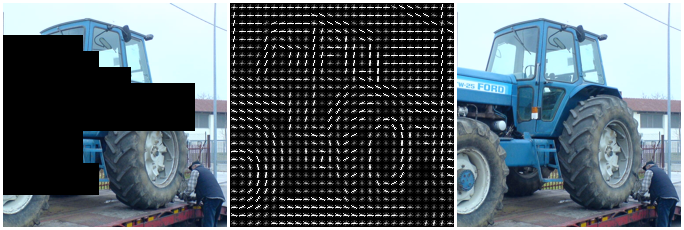
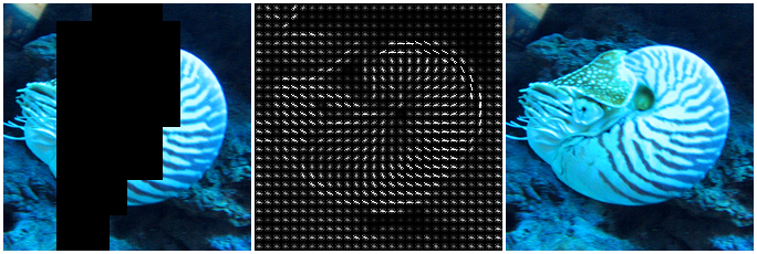
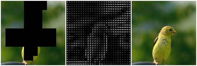
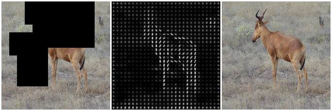
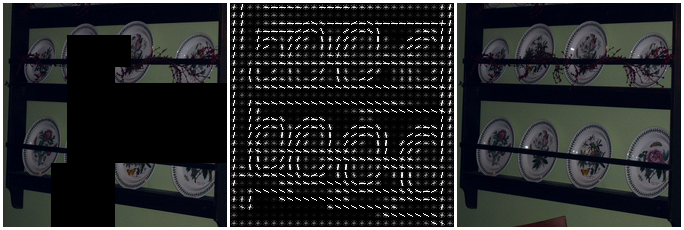
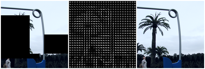
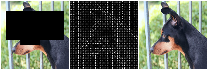
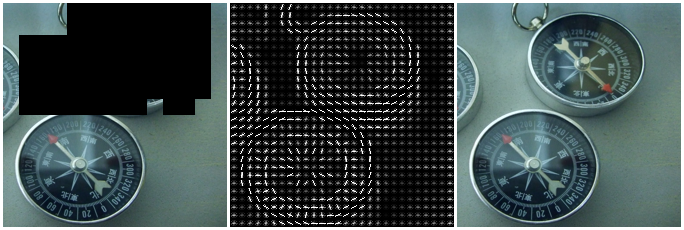
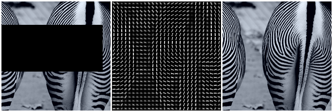
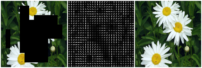
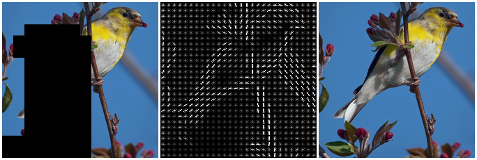
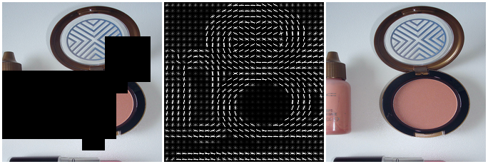
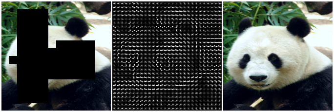
masked input

HOG prediction

original image

(a)

(b)

(c)

(d)

Figure 1: Example HOG predictions on unseen validation input. Our model is learned by predicting features (middle) given masked inputs (left). Original images (right) are not used for prediction. More qualitative examples for video and image are in Figs. 8 and 9.

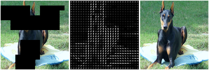
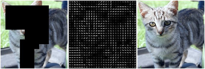
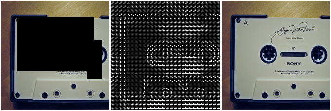
Self-supervised pre-training has been phenomenally successful in natural language processing powering large-scale Transformers [88] with billion-scale data [25, 6]. The underlying idea is an astonishingly simple mask-and-predict task, that is, first masking out some tokens within a text and then predicting the invisible content given the visible text.

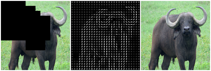
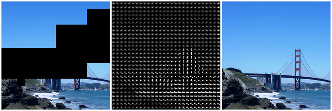
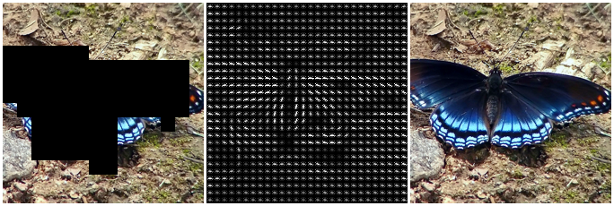
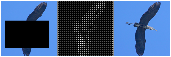
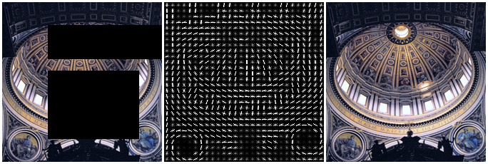
Humans have a remarkable ability to predict how the world appears and moves when observing it as a continuous stream of spatiotemporal information. Consider the examples in the 1 column of Fig. 1. Even without seeing the masked content, we are able to understand the object structure and draw a rough outline or silhouette of imagined information (up to some details), by using visual knowledge about the visible structures. In this work, we show that predicting certain masked features (e.g. gradient histograms in the 2 column) can be a powerful objective for self-supervised visual pre-training, especially in the video domain which contains rich visual information.

One essential difference between vision and language is that vision has no pre-existing vocabulary to shape the prediction task into a well-defined classification problem. In contrast, the raw spatiotemporal visual signal is continuous and dense posing a major challenge to masked visual prediction. One immediate solution is to imitate the language vocabulary by building a visual vocabulary that discretizes frame patches into tokens, as explored in BEiT [73, 2]. However, this requires an external tokenizer which can be limited in compute-intensive video understanding scenario.

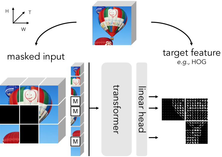
We present Masked Feature Prediction (MaskFeat), a pre-training objective that directly regresses features of the masked content. Specifically, our approach ingests the masked space-time input with a vision Transformer backbone [27, 56] and predicts a certain feature representation of the masked content. In this way, the pre-trained model acquires an adequate understanding of the complex space-time structures within dense visual signals.

We study a broad spectrum of feature types, from pixel colors and hand-crafted feature descriptors, to discrete visual tokens, activations of deep networks, and pseudo-labels from network predictions. Our study reveals:

(i) Simple histogram of oriented gradients (center column in Fig. 1), as in the popular HOG [22] and SIFT [62] descriptors which dominated visual recognition for over a decade, is a particularly effective target for MaskFeat in terms of both performance and efficiency.

(ii) The discretization (tokenization) of visual signals is not necessary for masked visual prediction, and continuous feature regression (i.e. MaskFeat) can work well.

(iii) Semantic knowledge from human annotations is not always helpful for MaskFeat, but characterizing local patterns seems important. For example, predicting supervised features from CNNs or ViTs trained on labeled data leads to degraded performance.

Our approach is conceptually and practically simple. Compared to contrastive methods that require a siamese structure and two or more views of each training sample (e.g., [44, 17, 34]), MaskFeat uses a single network with a single view of each sample; and unlike contrastive methods that strongly rely on carefully designed data augmentation, MaskFeat works fairly well with minimal augmentation.

Compared to previous masked visual prediction methods [2, 82], MaskFeat with HOG does not involve any external model, such as a dVAE tokenizer [73] that introduces not only an extra pre-training stage on 250M images, but also non-negligible training overhead in masked modeling.

We show that MaskFeat can pre-train large-scale video models that generalize well. Transformer-based video models, though powerful, are previously known to be prone to over-fitting and heavily rely on supervised pre-training [56, 1] on large-scale image datasets, e.g., ImageNet-21K (IN-21K) [24]. While MaskFeat opens the door for directly pre-training on unlabeled videos which shows enormous benefits for video understanding.

Our results on standard video benchmarks are groundbreaking: MaskFeat pre-trained MViT-L [56] gets 86.7% top-1 accuracy on Kinetics-400 [51] without using any external data, greatly surpassing the best prior number of this kind by +5.2%, and also methods using large-scale image datasets, e.g., IN-21K and JFT-300M [80]. When transferring to downstream tasks, MaskFeat gets unprecedented results of 39.8 mAP on action detection (AVA [42]) and 75.0% top-1 accuracy on human-object interaction classification (SSv2 [40]). When generalized to the image domain, MaskFeat also obtains competitive 84.0% top-1 with ViT-B and 85.7% with ViT-L using only ImageNet-1K [24].

Our code will be available in PyTorchVideo${}^{\text{,}}$ [30, 29].

Figure 2: MaskFeat pre-training. We randomly replace the input space-time cubes of a video with a [MASK] token and directly regress features (e.g. HOG) of the masked regions. After pre-training, the Transformer is fine-tuned on end tasks.

2 Method

We start by describing MaskFeat and its instantiations for video and image understanding in §2.1. We then introduce and discuss five candidates for target features in §2.2.

2.1 Masked Feature Prediction

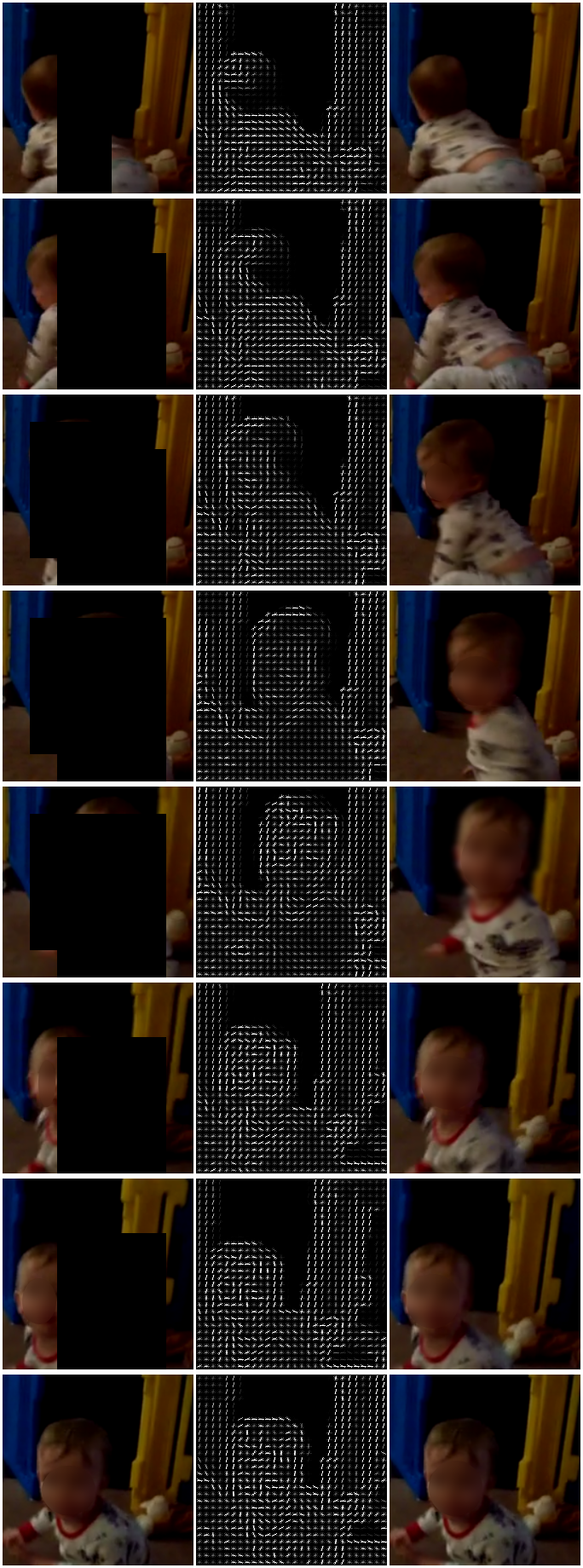
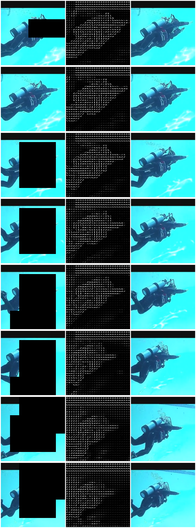
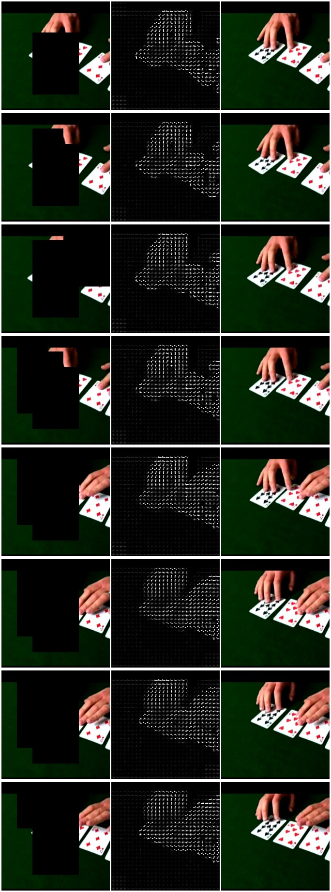
Our method performs a masked visual prediction task, motivated by humans’ ability to inpaint masked visual content up to some details. The task first randomly masks out a few space-time cubes of a video, and then predicts the masked ones given the remaining ones. By modeling masked samples, the model attains video understanding in the sense of recognizing parts and motion of objects. For instance, to solve the examples in Figs. 1 and 9, a model has to first recognize the objects based on the visible area, and also know what the objects typically appear and how they usually move to inpaint the missing area.

One key component of the task is the prediction target. Masked language modeling tokenizes the corpus with a vocabulary to serve as the target [25]. In contrast, the raw visual signal is continuous and high-dimensional and there is no natural vocabulary available. In MaskFeat, we propose to predict features of the masked area. And the supervision is provided by features extracted from the original, intact sample. We use a wide interpretation of features [13], from hand-crafted feature descriptors, to activations of deep networks. The choice of the target feature largely defines the task and impacts the property of the pre-trained model, which we discuss in §2.2.

Instantiations.

We first describe MaskFeat for video input.

A video is first divided into space-time cubes as in typical video Vision Transformers [31, 56]. The cubes are then projected (i.e. convolved) to a sequence of tokens. To perform masking, some of the tokens in the sequence are randomly masked out by being replaced with a [MASK] token. This is a learnable embedding indicating masked patches. A block of tokens is masked together which we detail in §4.3. To make a prediction, the token sequence after [MASK] token replacement, with positional embedding added, is processed by the Transformer. Output tokens corresponding to the masked cubes are projected to the prediction by a linear layer. The prediction is simply the feature of the 2-D spatial patch temporally centered in each masked cube (see discussions in § 4.3). The number of output channels is adjusted to the specific target feature (e.g., 3$\times$16$\times$16 if predicting RGB colors of pixels in a 16$\times$16 patch). The loss is only operated on the masked cubes. Our instantiation is inspired by BERT [25] and BEiT [2], illustrated in Fig. 2.

MaskFeat can be easily instantiated in the image domain, which can be interpreted as a video with one single frame. Most operations are shared, except that there is no temporal dimension and each token now represents only a spatial patch instead of a space-time cube.

2.2 Target Features

We consider five different types of target features. The targets are categorized into two groups: 1) one-stage targets that can be directly obtained including pixel colors and HOG, and 2) other two-stage targets extracted by a trained deep network or teacher. As predicting two-stage targets is effectively learning from a trained deep network teacher, it resembles a form of model distillation [48]; thereby, an extra computational cost of pre-training and inference of the teacher model is inevitable. The five feature types are:

Pixel colors.

The most straightforward target is arguably the colors of video pixels. Specifically, we use RGB values that are normalized by the mean and the standard deviation of the dataset. We minimize the $\ell_{2}$ distance between the model’s prediction and the ground-truth RGB values. A similar idea has been explored in [69] as a image inpainting task and in [2, 27] for masked image prediction. Though simple, pixels as target have a potential downside of overfitting to local statistics (e.g. illumination and contrast variations) and high-frequency details, which are presumably insignificant [76] for interpretation of visual content.

HOG.

Histograms of Oriented Gradients (HOG) [22] is a feature descriptor that describes the distribution of gradient orientations or edge directions within a local subregion. A HOG descriptor is implemented by a simple gradient filtering (i.e. subtracting neighboring pixels) to compute magnitudes and orientations of gradients at each pixel. The gradients within each small local subregion or cell are then accumulated into orientation histogram vectors of several bins, voted by gradient magnitudes. The histogram is normalized to unit length. These features are also used in well-known SIFT [62] descriptors for detected keypoints or in a dense fashion for classification [13]. Similarly, we extract HOG on a dense grid for the whole image, which suits the prediction target for randomly masked patches.

HOG is characteristic of capturing local shapes and appearances while being partially invariant to geometric changes as long as translations are within the spatial cell and rotations are smaller than orientation bin size. Further, it provides invariance to photometric changes as image gradients and local contrast normalization absorb brightness (e.g. illumination) and foreground-background contrast variation. These invariances are vital for good results when using HOG for pedestrian detection in both image [22] and video [23] domains. In accordance to this, our studies (§5.2) reveal local-contrast normalization in HOG is also essential for MaskFeat pre-training.

Finally, HOG computation is cheap and introduces negligible overhead. It can be implemented as a two-channel convolution to generate gradients in x and y axis (or by subtracting neighboring horizontal and vertical pixels) , followed by histogramming and normalization.

Our method then simply predicts the histograms summarizing masked patches. Instead of computing HOG only on masked patches, we first obtain a HOG feature map on the whole image and then split the map into patches. In this way, we reduce padding on boundaries of each masked patch. The histograms of masked patches are then flattened and concatenated into a 1-D vector as the target feature. Our loss minimizes the $\ell_{2}$ distance between the predicted and original HOG feature. We collect HOG in each RGB channel to include color information which can slightly improve its performance (§5.2).

(a)

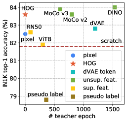
feature type	one-stage	variant	arch.	param.	epoch†	top-1
scratch	-	DeiT [84]	-	-	-	81.8
pixel colors	✓	RGB	-	-	-	82.5
image descriptor	✓	HOG [22]	-	-	-	83.6
dVAE token	✗	DALL-E [73]	dVAE	54	1199	82.8
unsupervised feature	✗	MoCo v2 [16]	ResNet50	23	800	83.6
unsupervised feature	✗	MoCo v3 [18]	ViT-B	85	600	83.9
unsupervised feature	✗	DINO [9]	ViT-B	85	1535	84.0
supervised feature	✗	pytorch [67]	ResNet50	23	90	82.6
supervised feature	✗	DeiT [84]	ViT-B	85	300	81.9
pseudo-label	✗	Token Labeling [50]	NFNet-F6	438	360	78.8

(b)

Table 2: Comparing target features for MaskFeat (image). For all targets, ViT-B is pre-trained with MaskFeat for 300 epochs on IN-1K. We report 100-epoch fine-tuning accuracy on IN-1K. For two-stage targets, we report the teacher architecture, number of parameters (M), and effective epoch^† on IN-1K. The default entry is marked in gray. The plot on the left visualizes the acc/epoch trade-off of the table.

^† Different teachers use different training strategies. dVAE is pre-trained on an external 250M dataset, while self-supervised methods require multi-view training. To measure the cost in a unified way, we normalize the number of epochs by the cost of one epoch on IN-1K training set with one 224² view.

Discrete variational autoencoder (dVAE).

To address the continuous high-dimensional nature of visual signals, DALL-E [73] proposes to compress an image with a dVAE codebook. In particular, each patch is encoded into a token which can assume 8192 possible values using a pre-trained dVAE model. Now the task is to predict the categorical distribution of the masked token by optimizing a cross-entropy loss, as explored in BEiT [2]. However, there is an extra computational cost induced by pre-training the dVAE and tokenizing images alongside masked feature prediction.

Deep features.

In comparison to discretized tokens, we consider directly using continuous deep network features as the prediction target. We use a pre-trained model to produce features as a teacher, either a CNN or ViT, and our loss minimizes the cosine distance (i.e. mean squared error of $\ell_{2}$-normalized features).

For CNN teachers, we use the last layers’ features corresponding to the masked patches and for ViT we use the respective output patch tokens. We mainly compare features from self-supervised models, which are considered to contain more diverse scene layout [9] and preserve more visual details [99] than features from supervised models. (Though, the usage of human annotations makes the pre-training technically not self-supervised.) Supervised features are expected to be more semantic as they are trained through human annotations. Similar to dVAE, a non-trivial amount of extra computation is involved when using extra model weights for masked feature generation.

Pseudo-label.

To explore an even more high-level semantic prediction target, we consider predicting class labels of masked patches. We utilize labels provided by Token Labeling [50], where each patch is assigned an individual location-specific IN-1K pseudo-label. This class label map is generated by a pre-trained high-performance supervised deep network [5] teacher. The masked feature prediction stage is optimized by a cross-entropy loss.

We next study the features discussed in this section.

3 Study: Target Features for MaskFeat

feature type	one-stage	variant	top-1
scratch	-	MViT-S [56]	81.1
pixel	✓	RGB	80.7
image descriptor	✓	HOG [22]	82.2
dVAE	✗	DALL-E [73]	81.7
unsupervised feature	✗	DINO [9], ViT-B	82.5
supervised feature	✗	MViT-B [31]	81.9

Table 1: Comparing target features for MaskFeat (video). All variants are pre-trained with MaskFeat for 300 epochs on MViT-S, 16$\times$4. We report fine-tuning accuracy on K400. Default is gray.

Settings.

We use a pre-training and fine-tuning protocol, following BEiT [2]. We pre-train MViT-S, 16$\times$4 [56] with MaskFeat on Kinetics-400 (K400) [51] training set for 300 epochs. We also apply MaskFeat on images, where we pre-train ViT-B [27] on the ImageNet-1K (IN-1K) [24] training set for 300 epochs. We report top-1 fine-tuning accuracy (%) on both datasets. We pre-train and fine-tune all targets with the same recipe which we find generally good in practice (§B.1). For targets that involve a teacher model, we use official models released by the authors.

Most features are compared on both video and image domains except pseudo-label for which the pseudo-label map is only available on IN-1K [50]. Results are summarized in Tables 1 (video) and 2 (image), analyzed next:

One-stage methods.

The fine-tuning accuracy for pixel color prediction in Tables  1 & 2 shows, that compared to the from-scratch baselines, regressing RGB colors produces a slight drop of -0.4% for video classification and a relatively small gain of +0.7% for image. Even though our predicting pixel colors result on IN-1K (82.5%) is better than that reported in BEiT [2] (81.0%), we similarly observe that pixel values are not ideal direct targets, presumably because they are considered to be too explicit [73]. In comparison, HOG, by summarizing the local gradient distribution, contributes to large improvements of +1.1% on K400 and +1.8% on IN-1K over the from-scratch baselines without any extra model which is typical in two-stage methods.

Two-stage methods.

First, dVAE improves by +0.6% for K400 and +1.0% for IN-1K over their from-scratch baselines. This is better than pixel colors, but outperformed by HOG which does not use an external model.

Next, compared to dVAE, we study MaskFeat to predict continuous, unsupervised features: We compare DINO [9] (with ViT-B) and MoCo [16, 18] (with ResNet50 [46] and ViT-B), all pre-trained on IN-1K, even for the video pre-training. Unsupervised features contribute a notable gain for both video and image classification: The DINO variant achieves a gain of +1.4% on K400 and +2.2% on IN-1K compared to their baselines. However, this approach has two main drawbacks, (i) the unsupervised feature extractor needs to be pre-trained e.g. worth over thousand epochs in the case of DINO, (ii) the unsupervised features need to be computed on the target data. Still, MaskFeat w/ DINO and MoCo v3 features boosts their original accuracy [9, 18].

Finally, supervised features (from ResNet50 or ViT-B) as well as token labels, though utilizing human annotations, lag behind unsupervised features and HOG. In fact, we notice significant over-fitting during fine-tuning for supervised features and token labels, suggesting that predicting features learned from class labels is not suitable in MaskFeat. We hypothesize that class label being invariant to local shapes and textures of the same object disables the ability of MaskFeat to model object’s internal structure.

Discussion.

Our results suggest that a broad spectrum of image features can serve as targets in masked visual prediction, and provide gains over the train-from-scratch baseline. We find that although masked language modeling [25] originally predicts the categorical distribution over a pre-defined vocabulary, discretization as in BEiT [2] is not required for vision. We find that continuous unsupervised features and image descriptors can be strong prediction targets, while the latter come without cost compared to the former which also entail a form of model distillation [49, 84]. An interesting observation is that supervisedly trained target features produce poor results, which might relate to class-level specific information being present in features [100, 3] that is too global for local mask modeling. Overall, considering the trade-off between performance and computational cost, predicting HOG holds a good balance and therefore we use it as default feature for MaskFeat in the following sections.

4 Experiments: Video Recognition

Settings.

We evaluate with base and large models of improved MViT [56]. The original MViT in [31] is termed as MViTv1. The models are pre-trained only on video clips in the training set of K400 [24] without labels. Our augmentation includes random resized cropping and horizontal flipping. Our models are pre-trained and fine-tuned at 224² resolution if not specified. We randomly mask out 40% of total space-time cubes with cube masking detailed in §4.3. More implementation details are in § B.1.

4.1 Main Results on Kinetics

Kinetics-400.

Table 3 compares MaskFeat with prior work on K400 dataset. From top to bottom, it has three sections.

The first section presents prior work using CNNs, which commonly do not use any pre-training. The second section presents representative Transformer-based methods, most of which are heavily dependent on supervised pre-training on large-scale image datasets.

The third section provides direct comparisons on MViT models. Note that these models are strong baselines and are state-of-the-art for training-from-scratch on their own. Still, 300 epochs of MaskFeat pre-training improve the scratch MViT-S, 16$\times$4 [56] with 81.1% top-1 accuracy by +1.1%. Here, the suffix 16$\times$4 represents that the model takes 16 frames with a temporal stride of 4 as input during training.

Next, we explore larger models for which supervised IN-21K pre-training is popular. Pre-trained with MaskFeat for 800 epochs on K400, the large model MViT-L, 16$\times$4 reaches 84.3% top-1, outperforming its scratch baseline by a large margin of +3.8% and its IN-21K supervised counterpart by +0.8%. Similar to the image domain, MaskFeat is more significant with larger models, showing that our approach is salable to model capacity. The result also suggests that MaskFeat adapts to different model types, as MViT is a Transformer model with convolutions. We provide ablation on the pre-training schedule in § 4.3.

We further explore the data scalability of MaskFeat. In particular, we pre-train MViT-L, 16$\times$4 with Kinetics-600 (K600) [10] containing ~387K training videos, 1.6$\times$ more than K400. We pre-train for 300 epochs on K600 to use a slightly smaller training budget as the 800 epochs on K400. We again fine-tune on K400 and observe that pre-training on K600, without any labels, contributes to another +0.8% gain over K400 pre-training to reach 85.1% top-1.

model	pre-train	top-1	top-5	FLOPs$\times$views	Param
Two-Stream I3D [12]	-	71.6	90.0	216 $\times$ NA	25
ip-CSN-152 [85]	-	77.8	92.8	109$\times$3$\times$10	33
SlowFast 16$\times$8 +NL [33]	-	79.8	93.9	234$\times$3$\times$10	60
X3D-XL [32]	-	79.1	93.9	48$\times$3$\times$10	11
MoViNet-A6 [53]	-	81.5	95.3	386$\times$1$\times$1	31
MViTv1-B, 64$\times$3 [31]	-	81.2	95.1	455$\times$3$\times$3	37
Swin-B, 32$\times$2 [59]	Sup., IN-21K	82.7	95.5	282$\times$3$\times$4	88
ViT-B-TimeSformer [4]	Sup., IN-21K	80.7	94.7	2380$\times$3$\times$1	121
Swin-L, 32$\times$2 [59]	Sup., IN-21K	83.1	95.9	604$\times$3$\times$4	197
ViViT-L [1]	Sup., JFT-300M	83.5	94.3	3980$\times$3$\times$1	308
Swin-L↑384, 32$\times$2 [59]	Sup., IN-21K	84.9	96.7	2107$\times$5$\times$10	200
ViViT-H [1]	Sup., JFT-300M	84.9	95.8	3981$\times$3$\times$4	654
TokenLearner [75]	Sup., JFT-300M	85.4	N/A	4076$\times$3$\times$4	450
Florence↑384 [95]	Text, FLD-900M	86.5	97.3	N/A$\times$3$\times$4	647
SwinV2-G↑384 [58]	MIM + Sup.	86.8	N/A	N/A$\times$5$\times$4	3000
	IN-21K+Ext-70M
MViT-S, 16$\times$4 [56]	-	81.1	94.9	71$\times$1$\times$10	36
MViT-S, 16$\times$4 [56]	Sup., IN-21K	82.6	95.3	71$\times$1$\times$10	36
MViT-S, 16$\times$4 [56]	MaskFeat, K400	82.2	95.1	71$\times$1$\times$10	36
MViT-L, 16$\times$4 [56]	-	80.5	94.1	377$\times$1$\times$10	218
MViT-L, 16$\times$4 [56]	Sup., IN-21K	83.5	95.9	377$\times$1$\times$10	218
MViT-L, 16$\times$4 [56]	MaskFeat, K400	84.3	96.3	377$\times$1$\times$10	218
MViT-L, 16$\times$4 [56]	MaskFeat, K600	85.1	96.6	377$\times$1$\times$10	218
MViT-L↑312, 32$\times$3 [56]	-	82.2	94.7	2063$\times$3$\times$5	218
MViT-L↑312, 32$\times$3 [56]	Sup., IN-21K	85.3	96.6	2063$\times$3$\times$5	218
MViT-L↑312, 32$\times$3 [56]	MaskFeat, K400	86.3	97.1	2063$\times$3$\times$5	218
MViT-L↑312, 40$\times$3 [56]	MaskFeat, K400	86.4	97.1	2828$\times$3$\times$4	218
MViT-L↑352, 40$\times$3 [56]	MaskFeat, K400	86.7	97.3	3790$\times$3$\times$4	218
MViT-L↑352, 40$\times$3 [56]	MaskFeat, K600	87.0	97.4	3790$\times$3$\times$4	218

Table 3: Comparison with previous work on Kinetics-400. We report the inference cost with a single “view” (temporal clip with spatial crop) $\times$ the number of views (FLOPs$\times$view${}_{\text{space}}$$\times$view${}_{\text{time}}$). Each “view” consists of $T$ frames with $\tau$ temporal stride, $T\times\tau$. Magnitudes are Giga ($10^{9}$) for FLOPs and Mega ($10^{6}$) for Param. Accuracy of models trained with external data is de-emphasized.

Next, we fine-tune the 84.3% top-1 MViT-L, 16$\times$4 MaskFeat model for 30 epochs to larger spatial sizes of 312² and 352², as well as longer temporal durations of 32 and 40 frames with a temporal stride of three. The resulting extra large model MViT-L↑352, 40$\times$3, without using any external data, achieves a top accuracy of 86.7%. Previously, Transformer-based video models heavily rely on supervised pre-training on large image datasets to reach high accuracy. For example, 84.9% top-1 Swin-L↑384 [59] with IN-21K and 84.9% ViViT-H [1] with JFT-300M [80]. MaskFeat opens the door for directly pre-training on unlabeled videos which shows enormous benefits for video understanding, as we can boost the previous best accuracy without external data on K400 (81.5% MoViNet-A6 [53]) by +5.2%.

Our best 87.0% top-1 accuracy is achieved by fine-tuning the 85.1% MViT-L, 16$\times$4 pre-trained with MaskFeat on 387K training videos in K600 using no labels.

Our results with just K400 (86.7%) is already similar to recent 86.5% Florence [95] and 86.8% SwinV2-G [58]. Florence uses 900M curated text-image pairs. SwinV2-G utilizes a giant model with three billion parameters, and is first self-supervisedly then supervisedly pre-trained on a large dataset of IN-21K plus 70M in-house images. The efficiency of our approach in terms of parameter count, compute cost, data, and annotation suggests again the advantage of MaskFeat directly pre-training on unlabeled videos.

model	pre-train	top-1	top-5	FLOPs$\times$views	Param
SlowFast 16$\times$8 +NL [33]	-	81.8	95.1	234$\times$3$\times$10	60
X3D-XL [32]	-	81.9	95.5	48$\times$3$\times$10	11
MoViNet-A6 [53]	-	84.8	96.5	386$\times$1$\times$1	31
MViTv1-B-24, 32$\times$3 [31]	-	84.1	96.5	236$\times$1$\times$5	53
Swin-B, 16$\times$2 [59]	Sup., IN-21K	84.0	96.5	282$\times$3$\times$4	88
Swin-L↑384, 32$\times$2 [59]	Sup., IN-21K	86.1	97.3	2107$\times$5$\times$10	200
ViViT-H [1]	Sup., JFT-300M	85.8	96.5	3981$\times$3$\times$4	654
Florence↑384 [95]	Text, FLD-900M	87.8	97.8	N/A$\times$3$\times$4	647
MViT-L, 16$\times$4 [56]	Sup., IN-21K	85.8	97.1	377$\times$1$\times$10	218
MViT-L, 16$\times$4 [56]	MaskFeat, K600	86.4	97.4	377$\times$1$\times$10	218
MViT-L↑312, 40$\times$3 [56]	Sup., IN-21K	87.5	97.8	2828$\times$3$\times$4	218
MViT-L↑312, 40$\times$3 [56]	MaskFeat, K600	88.3	98.0	2828$\times$3$\times$4	218

(a)

model	pre-train	top-1	top-5	FLOPs$\times$views	Param
SlowFast 16$\times$8 +NL [33]	-	71.0	89.6	234$\times$3$\times$10	60
MoViNet-A6 [53]	-	72.3	N/A	386$\times$1$\times$1	31
MViT-L, 16$\times$4 [56]	Sup., IN-21K	76.7	93.4	377$\times$1$\times$10	218
MViT-L, 16$\times$4 [56]	MaskFeat, K700	77.5	93.8	377$\times$1$\times$10	218
MViT-L↑312, 40$\times$3 [56]	Sup., IN-21K	79.4	94.9	2828$\times$3$\times$4	218
MViT-L↑312, 40$\times$3 [56]	MaskFeat, K700	80.4	95.7	2828$\times$3$\times$4	218

(b)

Table 4: Comparison with previous work on K600 & K700.

Kinetics-600 and Kinetics-700.

Table 4 compares with prior work on K600 [10] and K700 [11]. Both are larger versions of Kinetics. An MViT-L, 16$\times$4 is pre-trained with MaskFeat for 300 epochs and fine-tune for 75 epochs on both datasets. The models achieve the top accuracy of 86.4% on K600 and 77.5% on K700, using no external image data amd over 10$\times$fewer FLOPs compared to previous Transformer-based methods.

Finally, we fine-tune these MViT-L, 16$\times$4 models at a larger input resolution of 312 and a longer duration of 40$\times$3 to achieve 88.3% top-1 on K600 and 80.4% top-1 on K700, setting a new state-of-the-art with a large margin over the previous best approaches on each dataset, without any external supervised pre-training (e.g. on IN-21K or JFT-300M).

4.2 Transfer Learning

We evaluate transfer learning in downstream tasks using the MViT-L↑312, 40$\times$3 Kinetics models in Tables 3 and LABEL:tab:k600-finetune.

model	pre-train	center	full	FLOPs	Param
SlowFast R101, 8$\times$8 [33]	K400	23.8	-	138	53
MViTv1-B, 64$\times$3 [31]		27.3	-	455	36
SlowFast 16$\times$8 +NL [33]	K600	27.5	-	296	59
X3D-XL [32]		27.4	-	48	11
MViTv1-B-24, 32$\times$3 [31]		28.7	-	236	53
Object Transformer [92]		31.0	-	244	86
ACAR R101, 8$\times$8 +NL [66]		-	31.4	N/A	N/A
ACAR R101, 8$\times$8 +NL [66]	K700	-	33.3	N/A	N/A
MViT-L↑312, 40$\times$3 [56], Sup.	IN-21K+K400	31.6	-	2828	218
MViT-L↑312, 40$\times$3 [56], MaskFeat	K400	37.3	38.5	2828	218
MViT-L↑312, 40$\times$3 [56], MaskFeat	K600	38.8	39.8	2828	218

Table 5: Transferring to AVA v2.2 [42]. We use single center crop inference (center) following MViTv1 [31] and full resolution inference (full) to compare to the 2020 AVA Challenge winner ACAR [66]. Inference cost is with the center strategy.

Action detection.

AVA v2.2 [42] is a benchmark for spatiotemporal localization of human actions. We fine-tune the MViT-L↑312, 40$\times$3 Kinetics models on AVA v2.2. Details are in §B.2. Table 5 reports mean Average Precision (mAP) of our MaskFeat models compared with prior state-of-the-art. MaskFeat only using K400 contributes to a significant gain of +5.7 mAP over its IN-21K pre-trained counterpart using identical architectures. By utilizing a larger video dataset, K600, the model reaches an unprecedented accuracy of 39.8 mAP with full resolution testing, greatly surpassing all previous methods, including ActivityNet challenge winners. The strong performance of MaskFeat on AVA suggests a clear advantage of masked modeling on video over supervised classification on image pre-training for this localization-sensitive recognition task.

model	pre-train	top-1	top-5	FLOPs	Param
SlowFast, R101, 8$\times$8 [33]	K400	63.1	87.6	106	53
MViTv1-B, 64$\times$3 [31]		67.7	90.9	455	37
MViTv1-B-24, 32$\times$3 [31]	K600	68.7	91.5	236	53.2
Mformer-L [70]	IN-21K+K400	68.1	91.2	1185	109
ORViT Mformer-L [47]		69.5	91.5	1259	148
Swin-B, 32$\times$3 [59]		69.6	92.7	321	89
MViT-L↑312, 40$\times$3 [56], Sup.	IN-21K+K400	73.3	94.1	2828	218
MViT-L↑312, 40$\times$3 [56], MaskFeat	K400	74.4	94.6	2828	218
MViT-L↑312, 40$\times$3 [56], MaskFeat	K600	75.0	95.0	2828	218

Table 6: Transferring to Something-Something v2 [40]. We report FLOPs with a single “view”. All entries use one temporal clip and three spatial crops (inference cost is FLOPs$\times$3$\times$1).

Human-object interaction classification.

We fine-tune the MViT-L↑312, 40$\times$3 Kinetics models in Tables 3 and LABEL:tab:k600-finetune to Something-Something v2 (SSv2) [40] which focuses on human-object interaction classification. Table 6 presents the results and details are in § B.3. In contrast to Kinetics, SSv2 requires fine-grained motion distinctions and temporal modeling to distinguish interactions like picking something up and putting something down.

Despite the differences between the supervised tasks of Kinetics and SSv2, pre-training on Kinetics without supervised labels using MaskFeat still contributes to a large gain on fine-tuning accuracy of SSv2. Specifically, MaskFeat with only K400 data contributes to +1.1% top-1 over its IN-21K+K400 pre-trained counterpart. By utilizing the larger K600, the model reaches an unprecedented 75.0% top-1 accuracy, surpassing all previous methods. This suggests that MaskFeat can learn spatiotemporal representations from unlabeled Kinetics data which is known as appearance-biased, through self-supervised masked feature prediction.

4.3 Ablations for Video Recognition

The ablations are with MViT-S, 16$\times$4 pre-trained for 300 epochs on K400 if not specified. We report 200-epoch fine-tuning accuracy (%) on K400.

Masking strategy.

We study the masking strategy for spatiotemporal video data. In video, tokens sharing the same spatial position usually also share visual patterns. Therefore, we explore how to handle this redundancy brought by the addition of the temporal dimension. We consider three different ways of masking and present the results in Table 7. All entries share the same 40% masking ratio.

masking	frame	tube	cube
top-1	81.0 (-1.2)	81.9 (-0.3)	82.2

Table 7: Masking strategy. Varying the strategy of masking in spatiotemporal data. The default entry is highlighted in gray.

First, we consider “frame” masking, which independently masks out consecutive frames. This strategy mostly masks different spatial blocks in consecutive frames, but the model could temporally “interpolate” between frames to solve the task. This strategy only obtains 81.0% top-1.

Second, we consider “tube” masking. Namely, we first sample a 2-D mask map by block-wise masking as for images, and then extend the 2-D map by repeating it in the temporal dimension. Thus, the masked area is a straight tube in a video clip, in which the spatially masked area is the same for every frame. Tube masking refrains from relying on the temporal repetition to predict the masked content in static video. It leads to 81.9% accuracy.

Third, we consider “cube” masking, which includes both spatial and temporal blocks that are masked out. This is achieved by sampling random “cubes” of tokens until a certain masking ratio is reached. Cubes are sampled by first creating a 2-D block at a random time step, then extending in the temporal dimension with a random number of consecutive frames. Therefore, cube masking can be considered as an generalization of tube and frame masking. It produces 82.2% accuracy when used for pre-training.

Overall, the results in Table 7 show that cube masking performs best, suggesting both spatial and temporal cues are helpful in masked spatiotemporal prediction.

type	center patch	cube
top-1	82.2	82.0 (-0.2)

Table 8: Target design. Predicting center patch HOG or all HOG in a cube gives similar results. Default in gray.

Target design.

On video, each output token corresponds to a space-time cube. Our default setting is to simply predict the feature of the 2-D spatial patch temporally centered in each masked space-time cube. In Table 8 we consider another straightforward way of predicting the entire cube, i.e., HOG features of each 2-D patch in the 3-D cube. Results are similar and we use center patch prediction for simplicity.

ratio	20%	40%	60%	80%
top-1	81.9 (-0.3)	82.2	82.2	82.0 (-0.2)

Table 9: Masking ratio. Varying the percentage of masked patches. MaskFeat is robust to masking ratio in video domain.

Masking ratio.

We study the effect of the masking ratio in Table 9. Interestingly, a wide range of masking ratios from 40% to the extreme 80% can produce similar fine-tuning accuracy, and only a small ratio of 20% leads to a slight drop of -0.3%. This is different from the observation on images, where ratios larger than 40% lead to degraded accuracy (see discussions in Appendix A). This indicates that in the video domain visual patterns are indeed more redundant than in images, and thus MaskFeat enjoys a larger masking ratio to create a properly difficult task.

epoch	param. (M)	300	800
MViT-S, 16$\times$4	36	82.2	82.0 (-0.2)
MViT-L, 16$\times$4	218	83.1	84.3 (+1.2)

Table 10: Pre-training schedule. Large model benefits more from longer pre-training schedule.

Pre-training schedule.

We show different pre-training schedule lengths on K400 in Table 10. Each result is fine-tuned from a fully trained model instead of an intermediate checkpoint. For MViT-S with 36M parameters, extending pre-training from 300 epochs to 800 epochs results in a small performance degradation of 0.2% accuracy. In contrast, for MViT-L longer pre-training provides a significant gain of +1.2% accuracy. This suggests that MaskFeat is a scalable pre-training task that can be better utilized by models with larger capacity and longer schedule.

5 Experiments: Image Recognition

Settings.

The evaluation protocol is pre-training followed by end-to-end fine-tuning. We use vanilla base and large models in ViT [27] without modification. Our models are pre-trained at 224² resolution on IN-1K [24] training set without labels. We use minimal data augmentation: random resized cropping and horizontal flipping. We randomly mask out 40% of total image patches with block-wise masking following BEiT [2]. More details are in § B.1.

pre-train	extra data	extra model	ViT-B	ViT-L
scratch [84]	-	-	81.8	81.5
supervised384 [27]	IN-21K	-	84.0	85.2
MoCo v3 [18]	-	momentum ViT	83.2	84.1
DINO [9]	-	momentum ViT	82.8	-
BEiT [2]	DALL-E	dVAE	83.2	85.2
MaskFeat (w/ HOG)	-	-	84.0	85.7

Table 11: Comparison with previous work on IN-1K. All entries are pre-trained on IN-1K train split, except supervised₃₈₄ using IN-21K. MoCo v3 and DINO use momentum encoder. BEiT uses 250M DALL-E data to pre-train dVAE. All entries are trained and evaluated at image size 224² except supervised₃₈₄ at 384².

5.1 Main Results on ImageNet-1K

In Table 11 we compare MaskFeat to previous work including from-scratch, IN-21K supervised pre-training, and previous self-supervised methods. We pre-train MaskFeat for 1600 epochs here while for 300 epochs in Table 2. The fine-tuning schedule is the same everywhere and rather short, 100 epochs for ViT-B and 50 epochs for ViT-L.

We observe that MaskFeat pre-training significantly boosts the scratch baselines for both ViT-B and ViT-L. Our approach at image size 224² is on par with (ViT-B), or even outperforms (ViT-L) supervised pre-training on IN-21K that has 10$\times$more images and labels at image size 384². It has been shown [27] that ViT models are data-hungry and require large-scale supervised pre-training, possibly due to the lack of typical CNN inductive biases. Our results suggest that MaskFeat pre-training can overcome this without external labeled data by solving our feature inpainting task. Interestingly, more gains are observed on ViT-L compared with ViT-B, suggesting that it is scalable to larger models.

Compared to self-supervised pre-training approaches, MaskFeat is more accurate and simpler. MoCo v3 [18] and DINO [9] are contrastive methods that require multi-view training and carefully designed augmentation, while MaskFeat only uses single-views and minimal augmentation. See Appendix A for ablation on data augmentation of MaskFeat. Compared with BEiT [2], MaskFeat gets rid of the dVAE tokenizer, which introduces both an extra pre-training stage on the 250M DALL-E dataset, and a non-negligible inference overhead during masked prediction. While MaskFeat simply calculates HOG features.

MaskFeat in Table 11 is pre-trained for 1600 epochs with a single 224² view. DINO uses multiple global-local views and an extra momentum encoder, leading to 1535 effective epochs^† (Table 2). MoCo v3 saturates after 600 effective epochs [18]. BEiT is pre-trained for 800 epochs on IN-1K but requires another 1199 effective epochs for dVAE.

We also train the best model in Table 2, MaskFeat w/ DINO, for 1600 epochs and it reaches 84.2%; however, this uses a separate ViT-B model that is trained with another ~1535 effective epochs using DINO. MaskFeat w/ HOG can reach 84.0% without extra model.

5.2 Ablations for Image Recognition

We ablate the design choices of MaskFeat in the image domain first. We use ViT-B pre-trained for 300 epochs by default and report fine-tuning top-1 accuracy (%) on IN-1K. More ablations (e.g. on training epochs) are in Appendix A.

norm.	none	$\ell_{1}$	$\ell_{2}$
top-1	82.2	82.8	83.6

(a)

channel	gray	rgb	opp.
top-1	83.2	83.6	83.5

(b)

#bins	6	9	12
top-1	83.4	83.6	83.5

(c)

cell size	4$\times$4	8$\times$8	16$\times$16
top-1	83.2	83.6	83.2

(d)

Table 12: HOG implementation. LABEL:subtab:norm Local contrast normalization plays a key role, and LABEL:subtab:channel MaskFeat benefits from color information; this is in line with HOG/SIFT studies on image recognition [22, 13]. HOG as target is LABEL:subtab:nbins robust to the number of orientation bins, and LABEL:subtab:cellsize benefits from $8\times 8$ spatial cell. Opp. represents opponent color space [86]. Default entries are marked as gray.

HOG implementation.

We ablate HOG implementation details in Table 12. We first investigate the local contrast normalization in HOG, which is key to its performance in image recognition [22]. It is applied by normalizing each histogrammed vector of local 8$\times$8 pixel cells, which leads e.g. to local invariance in illumination change. We show in LABEL:subtab:norm that normalization is essential for MaskFeat. Compared with default $\ell_{2}$ normalization, using $\ell_{1}$ normalization results in a 0.8% drop and not using any normalization causes a large -1.4% drop. Similar results are reported in [22] for directly using HOG for image recognition.

We next investigate the effectiveness of color information in LABEL:subtab:channel. Gray corresponds to HOG on gray-scale images, which only contains intensity information. To include color information in HOG, rbg calculates separate gradients for each color channel and concatenates the three histograms. And opp. is an affine transformation of RGB to an opponent color space [86]. Results show that using color information provides a small gain of around +0.4% compared with only using gray-scaled intensity information.

We vary the number of orientation and spatial bins in LABEL:subtab:nbins and LABEL:subtab:cellsize, which provides geometric invariance in HOG descriptors. Following HOG[22], we use 9 orientation bins that are evenly spaced from 0° to 180° (unsigned), and use 8$\times$8 pixel cells (SIFT [62] uses 8 bins in 8$\times$8 cells). We observe that these default settings in [22] are good for MaskFeat and that it is robust to different numbers of orientation bins, but a specific size of 8$\times$8 pixels in a cell is the best.

 masked input  pixel prediction  HOG prediction  original image

(a)

(b)

(c)

(d)

Figure 6: Pixel vs. HOG predictions on IN-1K validation images^†. Pixel targets can have large errors for ambiguous problems, and HOG is more robust to ambiguity by histogramming and normalizing local gradients. Best viewed in color and zoomed in.

^† The unmasked regions are not used for loss and thus qualitatively poor.

Pixel vs. HOG.

We qualitatively compare HOG to pixel colors as the feature target of MaskFeat in Fig. 6. Both pixel and HOG predictions look reasonable in close proximity to the unmasked input. However, compared to HOG, pixel color targets come with more ambiguity. In the balloon (second) example, the model makes a sensible guess predicting a red balloon, which is black in the original image, resulting in a high loss penalty. In the sea urchin (third) example, the model is just able to make a blurry color-wise guess on the object, which is a natural consequence of minimizing a pixel-wise MSE loss in texture-rich, high-frequency regions [55]. In both cases, HOG reduces the risk of ambiguity: normalizing gradients handles the color ambiguity and spatial binning of gradients texture ambiguity.

targets	pixel	HOG	pixel + HOG
top-1	82.5 (-1.1)	83.6	82.3 (-1.3)

Table 13: Multi-tasking. Simply combining two targets with two separate linear prediction heads results in a drop, suggesting conflict in the objectives. The default entry is marked as gray.

Multi-tasking.

Finally, we investigate if combining different targets in a multi-task loss helps. Specifically, we combine pixel and HOG, two single-stage target features, by predicting each target with a separate linear layer. The two prediction losses are simply averaged with equal weighting. The results are summarized in Table 13. We see that multi-tasking of pixel and HOG provides a small gain over the scratch baseline (82.3% vs. 81.8%), but the accuracy is lower than pixel or HOG only. Though further tuning the loss weighting might improve this result, it signals that the two objectives can not benefit each other. This is reasonable, as HOG targets are locally normalized while pixel colors are strongly influenced by local brightness changes.

6 Related Work

Masked visual prediction

was pioneered with stacked autoencoders [89] and inpainting tasks[69] using ConvNets. Since the introduction of ViT [27], masked prediction has re-attracted attention of the vision community, partially inspired by the success of BERT [25] in NLP. BERT performs masked language modeling where some input tokens are masked at random and the task it to predict those. BERT pre-trained models scale well and generalize to a wide range of different downstream tasks.

For vision, different masked prediction objectives have been proposed. iGPT [14] predicts the next pixels of a sequence. ViT [27] predicts mean colors of masked patches. BEiT [2] and VIMPAC [82] encode masked patches with discrete variational autoencoder (dVAE) [87, 73]. Masked visual prediction has also been explored in the field of vision-language learning (e.g., [79, 63, 19, 52]). Compared to BEiT and VIMPAC, our method does not rely on dVAEs but directly regresses specific features of the input.

Self-supervised learning

aims to learn from unlabeled visual data by a pre-text task that is constructed by image/patch operations (e.g., [26, 65, 91, 98, 36, 7]) and spatiotemporal operations (e.g., [38, 64, 35, 68, 90]). Recently, contrastive learning [28] capitalizes on augmentation invariance. The invariance is achieved by enforcing similarity over distorted views of one image while avoiding model collapse [93, 44, 15, 8, 41, 9, 17, 72, 34]. The line of contrastive methods learns linearly separable representations, commonly evaluated by linear probing. While in this work we focus on maximizing model performance for the end task with an end-to-end fine-tuning protocol [2, 82].

7 Conclusion

We present Masked Feature Prediction (MaskFeat), a simple visual pre-training approach that regresses features of masked regions. In particular, HOG, a hand-designed feature that was driving visual recognition before the deep learning era, works surprisingly well as the prediction target. MaskFeat is efficient, generalizes well, and scales to large models for both video and image domains.

Our results are especially groundbreaking for video understanding: There has been a large gap of over 5% accuracy between supervised pre-training on large-scale image datasets and training-from-scratch methods. MaskFeat has closed this gap by directly pre-training on unlabeled videos. Transfer learning performance is even more impressive where an MaskFeat model surpasses its IN-21K counterpart, which uses 60$\times$ more labels, by +5.7 mAP on action detection (AVA) and +1.1% top-1 on human-object interaction recognition (SSv2). These results suggest a clear benefit of masked prediction in the visually richer space-time domain to explore in future work.

Appendix

In this Appendix, we provide further ablations for image (§A) classification. §B contains the implementation details, and §C provides more qualitative results.

Appendix A Ablations on Image Classification

epoch	300	800	1600
ViT-B	83.6	83.9 (+0.3)	84.0 (+0.4)
ViT-L	84.4	85.4 (+1.0)	85.7 (+1.3)

Table 14: Pre-training schedule. Gains with longer schedules are observed. The large model benefits more from longer schedules.

Pre-training schedule.

We show different lengths of pre-training in Table 14. Each result is fine-tuned from a fully trained model instead of an intermediate checkpoint.

For both base and large size models, improvements are observed with longer pre-training schedules. Interestingly, the large size model benefits more from longer pre-training with +1% gain from 300 epochs to 800 epochs, while the base-size model is only improved by +0.3%. This suggests that MaskFeat is a sufficiently difficult task such that (i) excessive long pre-training does not cause over-fitting of large models, and (ii) MaskFeat is sufficiently difficult for high capacity models. Training for 1600 epochs only gives another +0.1% improvement for ViT-B.

ratio	20%	40%	60%	80%
top-1	83.5 (-0.1)	83.6	83.1 (-0.5)	82.5 (-1.1)

Table 15: Masking ratio (image). Varying the percentage of masked patches. A smaller percentage of masking is preferred.

Masking ratio.

We vary the percentage of masked patches in Table 15 with block-wise masking following BEiT [2]. We observe that masking out 20%~40% patches works well and that stronger masking degrades accuracy. MaskFeat requires enough visible patches to set up a meaningful objective. Note that 20%~40% masking is more than 15% masking used in masked language modeling (BERT [25]), reflecting redundancy in raw visual signals.

aug.	RRC	RRC + color jit.	RRC + Rand Aug.
top-1	83.6	83.6	83.2 (-0.4)

(a)

scale	$[0.08,1.0]$	$[0.2,1.0]$	$[0.5,1.0]$	$[0.8,1.0]$
top-1	83.4 (-0.2)	83.4 (-0.2)	83.6	83.4 (-0.2)

(b)

Table 16: Data augmentation in MaskFeat. Defaults are gray.

Data augmentation.

We study the effect of data augmentation during MaskFeat pre-training in Table 16. All three entries in LABEL:subtab:aug use random horizontal flipping. Our approach works best with only random resized crop (RRC), while color jittering has no influence on the result and stronger augmentation (RandAugment [21]) degrades the performance slightly by 0.4%. This suggests that strong augmentations might lead to artificial patterns that in turn lead to a gap in pre-training and finetuning and MaskFeat works nearly augmentation-free. Conversely, contrastive-based methods are arguably dependent on “augmentation engineering” to provide prior knowledge (e.g., [16, 41]), which could lead to conflicting clues [71] and over-fitting to a specific combination of augmentations [94].

We further study the effect of the RRC $[\min,\max]$ scales in LABEL:subtab:rccscale. Our approach is robust to this hyper-parameter. MaskFeat works best with low strength of RRC, $[0.5,1.0]$, which covers a large fraction of each sample.

block	8	16	24
top-1	67.7	66.0	55.9

Table 17: Linear probing. We perform linear probing after the 8, 16, 24 (last) block of MaskFeat pre-trained ViT-L. Lower layers obtain better linear accuracy.

Linear probing.

Besides the fine-tuning protocol, we consider linear probing in Table 17 which is commonly used to evaluate contrastive methods [44, 15]. We train randomly initialized linear classifiers right at transformer block outputs. Specifically, we consider the average pooled outputs of the 8, 16 and 24 (last) transformer blocks of a ViT-L pre-trained with 1600 epochs of MaskFeat on IN-1K. We observe that lower layers (e.g., the 8) tend to have higher linear accuracy. This is different from contrastive based methods whose higher layers tend to obtain better linear accuracy [93, 83]. All layers lag behind contrastive methods by a large margin. For instance, MoCo v3 [18] has 77.6% at the last block of ViT-L. This suggests that contrastive-based and masked visual prediction methods have very different features. MaskFeat learns good visual knowledge revealed by fine-tuning protocol but not linearly separable features.

Our hypothesis here is that instance discrimination losses in contrastive learning create different embeddings (classes) for different images which can be largely reduced to class-level information (a subset of classes) with a linear layer.

config	ImageNet	Kinetics
optimizer	AdamW [61]
optimizer momentum	$\beta_{1},\beta_{2}{=}0.9,0.999$
weight decay	0.05
learning rate schedule	cosine decay [60]
warmup epochs [39]	30
augmentation	hflip, RandomResizedCrop
gradient clipping	0.02
drop path [54]	✗
base learning rate†	2e-4	8e-4
batch size	2048	512

(a)

config	ImageNet		Kinetics
	ViT-B	ViT-L	MViT-S	MViT-L
optimizer	AdamW [61]
optimizer momentum	$\beta_{1},\beta_{2}{=}0.9,0.999$
weight decay	0.05
learning rate schedule	cosine decay [60]
warmup epochs [39]	5
augmentation	RandAug (9, 0.5) [21]
mixup [97]	0.8
cutmix [96]	1.0
label smoothing [81]	0.1
drop out [78]	✗
base learning rate†	2e-3	1e-3	4.8e-3	9.6e-3
layer-wise decay [20]	0.65	0.75	0.75	0.875
batch size	2048	1024	512	256
training epochs	100	50	200	75
drop path [54]	0.1	0.1	0.1	0.2

(b)

Table 18: Configurations for ImageNet and Kinetics. ^†We use the linear lr scaling rule [39]: lr = base_lr$\times$batch_size / 256.

Appendix B Implementation Details

B.1 ImageNet and Kinetics Experiments

Architecture.

For ImageNet experiments, we use the standard ViT architecture [27] in base and large sizes. We use a single linear layer to transform the output of the last block to form the target predictions. We do not use relative positional bias or layer scaling.

For Kinetics experiments, we use the improved MViT architecture [56] and we term the original architecture in [31] as MViTv1. There are two main modifications. First, instead of using absolute positional embeddings as in MViTv1, relative positional embeddings [77] are incorporated, which are decomposed in height, width, and temporal axes. Second, a new residual pooling connection is introduced inside the attention blocks. Specifically, the pooled query tensor is added to the output sequence of self-attention. These two modifications improve the training-from-scratch and supervised-pre-trained baselines. We do not use channel dimension expansion within attention blocks [56] but at MLP outputs [31] which has similar accuracy. Our approach which focuses on pre-training techniques is orthogonal to these architectural modifications and provides further gains over the improved baselines.

Unlike ViT models sharing the spatial size of 14² for all blocks, the MViT architecture is multi-scale and has four scale stages. Stage 1 output is of spatial size 56² and stage 4 output is of spatial size 7². To share hyper-parameters with ViT models which are of spatial size 14², we remove MViTs’ query pooling before the last MViT stage for MaskFeat pre-training only, resulting in a 14² final output size, the same as ViT models. This modification introduces little extra computation as stage 4 is small and has only two Transformer blocks. For the fine-tuning stage, the MViT models are unchanged, with 7² output to fairly compare with the MViT baselines. Relative positional embeddings are linearly interpolated when the shape is not matched.

When sampling masked tokens for MViT models on the pre-training stage, we first sample a map of the final output size, 14². This masking map is then nearest-neighbor resized to the stage 1 size or input size, 56². In this way the set of input tokens corresponding to the same output token are masked out together, avoiding trivial predictions.

Pre-training.

LABEL:tab:detail_pt summarizes the pre-training configurations. Most of the configurations are shared by ImageNet and Kinetics, without specific tuning. This shows that MaskFeat is general across tasks. The gradient clipping value is set after monitoring training loss over short runs. It is 0.02 for HOG targets and 0.3 for pixel color prediction and deep feature targets.

Fine-tuning.

LABEL:tab:detail_ft summarizes the fine-tuning configurations. Most of the configurations are shared across models, except that deeper models use larger layer-wise learning rate decay and larger drop path rates.

For extra-large, long-term video models with 312 and 352 spatial resolutions as well as 32$\times$3 and 40$\times$3 temporal durations, we initialize from their 224 resolution, 16$\times$4 duration counterparts, disable mixup, and fine-tune for 30 epochs with a learning rate of 1.6e-5 at batch size 128, a weight decay of 1e-8, a drop path [54] rate of 0.75 and a drop out rate of 0.5 for the final linear projection. Other parameters are shared with LABEL:tab:detail_ft.

B.2 AVA Experiments

The AVA action detection dataset [42] assesses the spatiotemporal localization of human actions in videos. It has 211K training and 57K validation video segments. We evaluate methods on AVA v2.2 and use mean Average Precision (mAP) on 60 classes as is standard in prior work [33].

We use MViT-L↑312, 40$\times$3 as the backbone and follow the same detection architecture in [33, 31, 56] that adapts Faster R-CNN [74] for video action detection. Specifically, we extract region-of-interest (RoI) features [37] by frame-wise RoIAlign [45] on the spatiotemporal feature maps from the last MViT layer. The RoI features are then max-pooled and fed to a per-class sigmoid classifier for action prediction. The training recipe is identical to [31, 56] and summarized next. The region proposals are identical to the ones used in [33, 31, 56]. We use proposals that have overlaps with ground-truth boxes by IoU $>$ 0.9 for training. The models are trained with synchronized SGD training with a batch size of 64. The base learning rate is 0.6 per 64 batch size with cosine decay [60]. We train for 30 epochs with linear warm-up [39] for the first five epochs and use a weight decay of 1e-8, a drop path of 0.4 and a head dropout of 0.5.

B.3 SSv2 Experiments

The SSv2 dataset [40] contains 169K training, and 25K validation videos with 174 human-object interaction classes. We fine-tune the pre-trained MViT-L↑312, 40$\times$3 Kinetics models and take the same recipe as in [31, 56]. Specifically, we train for 40 epochs with a batch size of 128. The base learning rate is 0.02 per 128 batch size with cosine decay [60]. We adopt synchronized SGD and use weight decay of 1e-4 and drop path rate of 0.75. The training augmentation is the same as Kinetics in LABEL:tab:detail_ft, except we disable random flipping in training. We use the segment-based input frame sampling [31, 57] (split each video into segments, and sample one frame from each segment to form a clip). During inference, we take a single temporal clip and three spatial crops over a single video.

Appendix C Qualitative Experiments

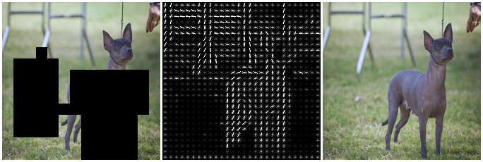
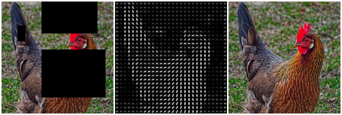
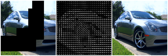
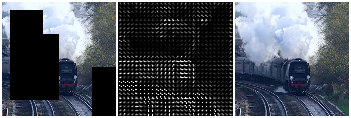
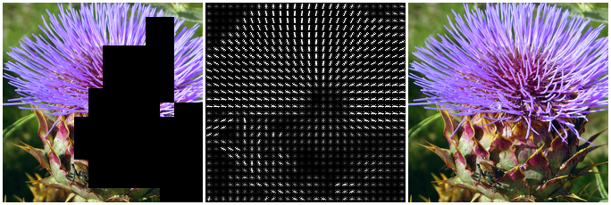
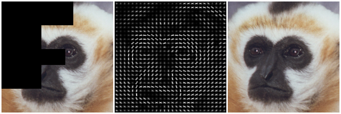
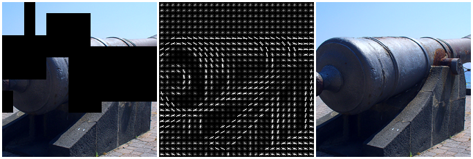
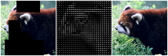
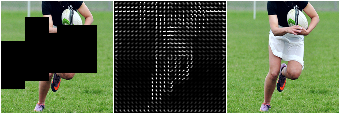
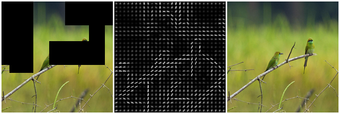
We provide more qualitative results of image HOG predictions in Fig. 8 using ImageNet-1K validation images and for video HOG predictions in Fig. 9 using Kinetics-400 validation videos.

Figure 8: More visualizations of HOG predictions. The images are from IN-1K validation set. For each column, we show masked input (left), HOG predictions (middle) and original images (right). Original images are not used for prediction. Best viewed in color with zoom.

Figure 9: More visualizations of HOG predictions (video). The video clips are from K400 validation set. For each column, we show masked input (left), HOG predictions (middle) and original video frames (right), and we show eight frames from top to bottom. Original video clips are not used for prediction. Best viewed in color with zoom.

Appendix D Acknowledgement

This project was partially influenced by initial signals of the MAE project [43]. We thank Kaiming He and Huiyu Wang for feedback on the manuscript.

Appendix E Changes in arXiv v2

We update MaskFeat AVA results in Table 5 according to the changes in the official AVA evaluation code. The evaluated models are unchanged.

model	pre-train	center	full	version
MViT-L↑312, 40$\times$3 [56], MaskFeat	K400	36.3	37.5	v1
MViT-L↑312, 40$\times$3 [56], MaskFeat	K600	37.8	38.8	v1
MViT-L↑312, 40$\times$3 [56], MaskFeat	K400	37.3	38.5	v2
MViT-L↑312, 40$\times$3 [56], MaskFeat	K600	38.8	39.8	v2

Table 19: Updated AVA results in Table 5 according to changes in the official AVA evaluation code. The models are unchanged.

References

- [1] Anurag Arnab, Mostafa Dehghani, Georg Heigold, Chen Sun, Mario Lučić, and Cordelia Schmid. ViViT: A video vision transformer. In ICCV, 2021.
- [2] Hangbo Bao, Li Dong, and Furu Wei. BEiT: BERT pre-training of image transformers. arXiv preprint arXiv:2106.08254, 2021.
- [3] David Bau, Bolei Zhou, Aditya Khosla, Aude Oliva, and Antonio Torralba. Network dissection: Quantifying interpretability of deep visual representations. In CVPR, 2017.
- [4] Gedas Bertasius, Heng Wang, and Lorenzo Torresani. Is space-time attention all you need for video understanding? In ICML, 2021.
- [5] Andrew Brock, Soham De, Samuel L Smith, and Karen Simonyan. High-performance large-scale image recognition without normalization. In ICML, 2021.
- [6] Tom B. Brown, Benjamin Mann, Nick Ryder, Melanie Subbiah, Jared Kaplan, Prafulla Dhariwal, Arvind Neelakantan, Pranav Shyam, Girish Sastry, Amanda Askell, Sandhini Agarwal, Ariel Herbert-Voss, Gretchen Krueger, Tom Henighan, Rewon Child, Aditya Ramesh, Daniel M. Ziegler, Jeffrey Wu, Clemens Winter, Christopher Hesse, Mark Chen, Eric Sigler, Mateusz Litwin, Scott Gray, Benjamin Chess, Jack Clark, Christopher Berner, Sam McCandlish, Alec Radford, Ilya Sutskever, and Dario Amodei. Language models are few-shot learners. In NeurIPS, 2020.
- [7] Mathilde Caron, Piotr Bojanowski, Armand Joulin, and Matthijs Douze. Deep clustering for unsupervised learning of visual features. In ECCV, 2018.
- [8] Mathilde Caron, Ishan Misra, Julien Mairal, Priya Goyal, Piotr Bojanowski, and Armand Joulin. Unsupervised learning of visual features by contrasting cluster assignments. In NeurIPS, 2020.
- [9] Mathilde Caron, Hugo Touvron, Ishan Misra, Hervé Jégou, Julien Mairal, Piotr Bojanowski, and Armand Joulin. Emerging properties in self-supervised vision transformers. In ICCV, 2021.
- [10] Joao Carreira, Eric Noland, Andras Banki-Horvath, Chloe Hillier, and Andrew Zisserman. A short note about kinetics-600. arXiv preprint arXiv:1808.01340, 2018.
- [11] Joao Carreira, Eric Noland, Chloe Hillier, and Andrew Zisserman. A short note on the kinetics-700 human action dataset. arXiv preprint arXiv:1907.06987, 2019.
- [12] Joao Carreira and Andrew Zisserman. Quo vadis, action recognition? a new model and the kinetics dataset. In CVPR, 2017.
- [13] Ken Chatfield, Karen Simonyan, Andrea Vedaldi, and Andrew Zisserman. Return of the devil in the details: Delving deep into convolutional nets. In BMVC, 2014.
- [14] Mark Chen, Alec Radford, Rewon Child, Jeff Wu, Heewoo Jun, Prafulla Dhariwal, David Luan, and Ilya Sutskever. Generative pretraining from pixels. In ICML, 2020.
- [15] Ting Chen, Simon Kornblith, Mohammad Norouzi, and Geoffrey Hinton. A simple framework for contrastive learning of visual representations. In ICML, 2020.
- [16] Xinlei Chen, Haoqi Fan, Ross Girshick, and Kaiming He. Improved baselines with momentum contrastive learning. arXiv preprint arXiv:2003.04297, 2020.
- [17] Xinlei Chen and Kaiming He. Exploring simple siamese representation learning. In CVPR, 2021.
- [18] Xinlei Chen, Saining Xie, and Kaiming He. An empirical study of training self-supervised vision transformers. In ICCV, 2021.
- [19] Yen-Chun Chen, Linjie Li, Licheng Yu, Ahmed El Kholy, Faisal Ahmed, Zhe Gan, Yu Cheng, and Jingjing Liu. Uniter: Universal image-text representation learning. In ECCV, 2020.
- [20] Kevin Clark, Minh-Thang Luong, Quoc V Le, and Christopher D Manning. ELECTRA: Pre-training text encoders as discriminators rather than generators. In ICLR, 2020.
- [21] Ekin D Cubuk, Barret Zoph, Jonathon Shlens, and Quoc V Le. RandAugment: Practical automated data augmentation with a reduced search space. In CVPR, 2020.
- [22] Navneet Dalal and Bill Triggs. Histograms of oriented gradients for human detection. In CVPR, 2005.
- [23] Navneet Dalal, Bill Triggs, and Cordelia Schmid. Human detection using oriented histograms of flow and appearance. In ECCV, 2006.
- [24] Jia Deng, Wei Dong, Richard Socher, Li-Jia Li, Kai Li, and Li Fei-Fei. ImageNet: A large-scale hierarchical image database. In CVPR, 2009.
- [25] Jacob Devlin, Ming-Wei Chang, Kenton Lee, and Kristina Toutanova. BERT: Pre-training of deep bidirectional transformers for language understanding. In NAACL, 2019.
- [26] Carl Doersch, Abhinav Gupta, and Alexei A Efros. Unsupervised visual representation learning by context prediction. In ICCV, 2015.
- [27] Alexey Dosovitskiy, Lucas Beyer, Alexander Kolesnikov, Dirk Weissenborn, Xiaohua Zhai, Thomas Unterthiner, Mostafa Dehghani, Matthias Minderer, Georg Heigold, Sylvain Gelly, Jakob Uszkoreit, and Neil Houlsby. An image is worth 16x16 words: Transformers for image recognition at scale. In ICLR, 2021.
- [28] Alexey Dosovitskiy, Philipp Fischer, Jost Tobias Springenberg, Martin Riedmiller, and Thomas Brox. Discriminative unsupervised feature learning with exemplar convolutional neural networks. TPAMI, 2015.
- [29] Haoqi Fan, Yanghao Li, Bo Xiong, Wan-Yen Lo, and Christoph Feichtenhofer. PySlowFast. https://github.com/facebookresearch/slowfast, 2020.
- [30] Haoqi Fan, Tullie Murrell, Heng Wang, Kalyan Vasudev Alwala, Yanghao Li, Yilei Li, Bo Xiong, Nikhila Ravi, Meng Li, Haichuan Yang, Jitendra Malik, Ross Girshick, Matt Feiszli, Aaron Adcock, Wan-Yen Lo, and Christoph Feichtenhofer. PyTorchVideo: A deep learning library for video understanding. In ACM MM, 2021. https://pytorchvideo.org/.
- [31] Haoqi Fan, Bo Xiong, Karttikeya Mangalam, Yanghao Li, Zhicheng Yan, Jitendra Malik, and Christoph Feichtenhofer. Multiscale vision transformers. In ICCV, 2021.
- [32] Christoph Feichtenhofer. X3D: Expanding architectures for efficient video recognition. In CVPR, 2020.
- [33] Christoph Feichtenhofer, Haoqi Fan, Jitendra Malik, and Kaiming He. Slowfast networks for video recognition. In ICCV, 2019.
- [34] Christoph Feichtenhofer, Haoqi Fan, Bo Xiong, Ross Girshick, and Kaiming He. A large-scale study on unsupervised spatiotemporal representation learning. In CVPR, 2021.
- [35] Basura Fernando, Hakan Bilen, Efstratios Gavves, and Stephen Gould. Self-supervised video representation learning with odd-one-out networks. In CVPR, 2017.
- [36] Spyros Gidaris, Praveer Singh, and Nikos Komodakis. Unsupervised representation learning by predicting image rotations. In ICLR, 2018.
- [37] Ross Girshick. Fast R-CNN. In ICCV, 2015.
- [38] Ross Goroshin, Joan Bruna, Jonathan Tompson, David Eigen, and Yann LeCun. Unsupervised learning of spatiotemporally coherent metrics. In ICCV, 2015.
- [39] Priya Goyal, Piotr Dollár, Ross Girshick, Pieter Noordhuis, Lukasz Wesolowski, Aapo Kyrola, Andrew Tulloch, Yangqing Jia, and Kaiming He. Accurate, large minibatch SGD: Training imagenet in 1 hour. arXiv preprint arXiv:1706.02677, 2017.
- [40] Raghav Goyal, Samira Ebrahimi Kahou, Vincent Michalski, Joanna Materzynska, Susanne Westphal, Heuna Kim, Valentin Haenel, Ingo Fruend, Peter Yianilos, Moritz Mueller-Freitag, et al. The “something something” video database for learning and evaluating visual common sense. In ICCV, 2017.
- [41] Jean-Bastien Grill, Florian Strub, Florent Altché, Corentin Tallec, Pierre H. Richemond, Elena Buchatskaya, Carl Doersch, Bernardo Avila Pires, Zhaohan Daniel Guo, Mohammad Gheshlaghi Azar, Bilal Piot, Koray Kavukcuoglu, Rémi Munos, and Michal Valko. Bootstrap your own latent: A new approach to self-supervised learning. In NeruIPS, 2020.
- [42] Chunhui Gu, Chen Sun, Sudheendra Vijayanarasimhan, Caroline Pantofaru, David A. Ross, George Toderici, Yeqing Li, Susanna Ricco, Rahul Sukthankar, Cordelia Schmid, and Jitendra Malik. AVA: A video dataset of spatio-temporally localized atomic visual actions. In CVPR, 2018.
- [43] Kaiming He, Xinlei Chen, Saining Xie, Yanghao Li, Piotr Dollár, and Ross Girshick. Masked autoencoders are scalable vision learners. arXiv preprint arXiv:2111.06377, 2021.
- [44] Kaiming He, Haoqi Fan, Yuxin Wu, Saining Xie, and Ross Girshick. Momentum contrast for unsupervised visual representation learning. In CVPR, 2020.
- [45] Kaiming He, Georgia Gkioxari, Piotr Dollár, and Ross Girshick. Mask R-CNN. In ICCV, 2017.
- [46] Kaiming He, Xiangyu Zhang, Shaoqing Ren, and Jian Sun. Deep residual learning for image recognition. In CVPR, 2016.
- [47] Roei Herzig, Elad Ben-Avraham, Karttikeya Mangalam, Amir Bar, Gal Chechik, Anna Rohrbach, Trevor Darrell, and Amir Globerson. Object-region video transformers. arXiv preprint arXiv:2110.06915, 2021.
- [48] Geoffrey Hinton, Oriol Vinyals, and Jeff Dean. Distilling the knowledge in a neural network. In NeurIPS, 2015.
- [49] Geoffrey Hinton, Oriol Vinyals, and Jeff Dean. Distilling the knowledge in a neural network. arXiv preprint arXiv:1503.02531, 2015.
- [50] Zihang Jiang, Qibin Hou, Li Yuan, Daquan Zhou, Yujun Shi, Xiaojie Jin, Anran Wang, and Jiashi Feng. All tokens matter: Token labeling for training better vision transformers. In NeurIPS, 2021.
- [51] Will Kay, Joao Carreira, Karen Simonyan, Brian Zhang, Chloe Hillier, Sudheendra Vijayanarasimhan, Fabio Viola, Tim Green, Trevor Back, Paul Natsev, et al. The kinetics human action video dataset. arXiv preprint arXiv:1705.06950, 2017.
- [52] Wonjae Kim, Bokyung Son, and Ildoo Kim. ViLT: Vision-and-language transformer without convolution or region supervision. In ICML, 2021.
- [53] Dan Kondratyuk, Liangzhe Yuan, Yandong Li, Li Zhang, Mingxing Tan, Matthew Brown, and Boqing Gong. MoviNets: Mobile video networks for efficient video recognition. In CVPR, 2021.
- [54] Gustav Larsson, Michael Maire, and Gregory Shakhnarovich. FractalNet: Ultra-deep neural networks without residuals. In ICLR, 2017.
- [55] Christian Ledig, Lucas Theis, Ferenc Huszár, Jose Caballero, Andrew Cunningham, Alejandro Acosta, Andrew Aitken, Alykhan Tejani, Johannes Totz, Zehan Wang, et al. Photo-realistic single image super-resolution using a generative adversarial network. In CVPR, 2017.
- [56] Yanghao Li, Chao-Yuan Wu, Haoqi Fan, Karttikeya Mangalam, Bo Xiong, Jitendra Malik, and Christoph Feichtenhofer. Improved multiscale vision transformers for classification and detection. arXiv preprint arXiv:2112.01526, 2021.
- [57] Ji Lin, Chuang Gan, and Song Han. TSM: Temporal shift module for efficient video understanding. In ICCV, 2019.
- [58] Ze Liu, Han Hu, Yutong Lin, Zhuliang Yao, Zhenda Xie, Yixuan Wei, Jia Ning, Yue Cao, Zheng Zhang, Li Dong, Furu Wei, and Baining Guo. Swin transformer v2: Scaling up capacity and resolution. arXiv preprint arXiv:2111.09883, 2021.
- [59] Ze Liu, Jia Ning, Yue Cao, Yixuan Wei, Zheng Zhang, Stephen Lin, and Han Hu. Video swin transformer. arXiv preprint arXiv:2106.13230, 2021.
- [60] Ilya Loshchilov and Frank Hutter. SGDR: Stochastic gradient descent with warm restarts. In ICLR, 2017.
- [61] Ilya Loshchilov and Frank Hutter. Decoupled weight decay regularization. In ICLR, 2019.
- [62] David G Lowe. Object recognition from local scale-invariant features. In ICCV, 1999.
- [63] Jiasen Lu, Dhruv Batra, Devi Parikh, and Stefan Lee. ViLBERT: Pretraining task-agnostic visiolinguistic representations for vision-and-language tasks. In NeurIPS, 2019.
- [64] Ishan Misra, C Lawrence Zitnick, and Martial Hebert. Shuffle and learn: unsupervised learning using temporal order verification. In ECCV, 2016.
- [65] Mehdi Noroozi and Paolo Favaro. Unsupervised learning of visual representations by solving jigsaw puzzles. In ECCV, 2016.
- [66] Junting Pan, Siyu Chen, Mike Zheng Shou, Yu Liu, Jing Shao, and Hongsheng Li. Actor-context-actor relation network for spatio-temporal action localization. In CVPR, 2021.
- [67] Adam Paszke, Sam Gross, Francisco Massa, Adam Lerer, James Bradbury, Gregory Chanan, Trevor Killeen, Zeming Lin, Natalia Gimelshein, Luca Antiga, Alban Desmaison, Andreas Kopf, Edward Yang, Zachary DeVito, Martin Raison, Alykhan Tejani, Sasank Chilamkurthy, Benoit Steiner, Lu Fang, Junjie Bai, and Soumith Chintala. PyTorch: An imperative style, high-performance deep learning library. In NeurIPS, 2019.
- [68] Deepak Pathak, Ross Girshick, Piotr Dollár, Trevor Darrell, and Bharath Hariharan. Learning features by watching objects move. In CVPR, 2017.
- [69] Deepak Pathak, Philipp Krahenbuhl, Jeff Donahue, Trevor Darrell, and Alexei A Efros. Context encoders: Feature learning by inpainting. In CVPR, 2016.
- [70] Mandela Patrick, Dylan Campbell, Yuki M. Asano, Ishan Misra Florian Metze, Christoph Feichtenhofer, Andrea Vedaldi, and João F. Henriques. Keeping your eye on the ball: Trajectory attention in video transformers. In NeurIPS, 2021.
- [71] Senthil Purushwalkam and Abhinav Gupta. Demystifying contrastive self-supervised learning: Invariances, augmentations and dataset biases. In NeurIPS, 2020.
- [72] Rui Qian, Tianjian Meng, Boqing Gong, Ming-Hsuan Yang, Huisheng Wang, Serge Belongie, and Yin Cui. Spatiotemporal contrastive video representation learning. In CVPR, 2021.
- [73] Aditya Ramesh, Mikhail Pavlov, Gabriel Goh, Scott Gray, Chelsea Voss, Alec Radford, Mark Chen, and Ilya Sutskever. Zero-shot text-to-image generation. In ICML, 2021.
- [74] Shaoqing Ren, Kaiming He, Ross Girshick, and Jian Sun. Faster R-CNN: Towards real-time object detection with region proposal networks. In NeurIPS, 2015.
- [75] Michael S Ryoo, AJ Piergiovanni, Anurag Arnab, Mostafa Dehghani, and Anelia Angelova. Tokenlearner: What can 8 learned tokens do for images and videos? arXiv preprint arXiv:2106.11297, 2021.
- [76] Tim Salimans, Ian Goodfellow, Wojciech Zaremba, Vicki Cheung, Alec Radford, and Xi Chen. Improved techniques for training GANs. In NeurIPS, 2016.
- [77] Peter Shaw, Jakob Uszkoreit, and Ashish Vaswani. Self-attention with relative position representations. arXiv preprint arXiv:1803.02155, 2018.
- [78] Nitish Srivastava, Geoffrey Hinton, Alex Krizhevsky, Ilya Sutskever, and Ruslan Salakhutdinov. Dropout: A simple way to prevent neural networks from overfitting. JMLR, 2014.
- [79] Weijie Su, Xizhou Zhu, Yue Cao, Bin Li, Lewei Lu, Furu Wei, and Jifeng Dai. VL-BERT: Pre-training of generic visual-linguistic representations. In ICLR, 2020.
- [80] Chen Sun, Abhinav Shrivastava, Saurabh Singh, and Abhinav Gupta. Revisiting unreasonable effectiveness of data in deep learning era. In ICCV, 2017.
- [81] Christian Szegedy, Vincent Vanhoucke, Sergey Ioffe, Jon Shlens, and Zbigniew Wojna. Rethinking the inception architecture for computer vision. In CVPR, 2016.
- [82] Hao Tan, Jie Lei, Thomas Wolf, and Mohit Bansal. VIMPAC: Video pre-training via masked token prediction and contrastive learning. arXiv preprint arXiv:2106.11250, 2021.
- [83] Yonglong Tian, Dilip Krishnan, and Phillip Isola. Contrastive multiview coding. In ECCV, 2020.
- [84] Hugo Touvron, Matthieu Cord, Matthijs Douze, Francisco Massa, Alexandre Sablayrolles, and Herve Jegou. Training data-efficient image transformers & distillation through attention. In ICML, 2021.
- [85] Du Tran, Heng Wang, Lorenzo Torresani, and Matt Feiszli. Video classification with channel-separated convolutional networks. In ICCV, 2019.
- [86] Koen Van De Sande, Theo Gevers, and Cees Snoek. Evaluating color descriptors for object and scene recognition. TPAMI, 2009.
- [87] Aaron van den Oord, Oriol Vinyals, and Koray Kavukcuoglu. Neural discrete representation learning. In NeurIPS, 2017.
- [88] Ashish Vaswani, Noam Shazeer, Niki Parmar, Jakob Uszkoreit, Llion Jones, Aidan N Gomez, Łukasz Kaiser, and Illia Polosukhin. Attention is all you need. In NeurIPS, 2017.
- [89] Pascal Vincent, Hugo Larochelle, Isabelle Lajoie, Yoshua Bengio, Pierre-Antoine Manzagol, and Léon Bottou. Stacked denoising autoencoders: Learning useful representations in a deep network with a local denoising criterion. JMLR, 2010.
- [90] Xiaolong Wang, Kaiming He, and Abhinav Gupta. Transitive invariance for self-supervised visual representation learning. In ICCV, 2017.
- [91] Chen Wei, Lingxi Xie, Xutong Ren, Yingda Xia, Chi Su, Jiaying Liu, Qi Tian, and Alan L Yuille. Iterative reorganization with weak spatial constraints: Solving arbitrary jigsaw puzzles for unsupervised representation learning. In CVPR, 2019.
- [92] Chao-Yuan Wu and Philipp Krahenbuhl. Towards long-form video understanding. In CVPR, 2021.
- [93] Zhirong Wu, Yuanjun Xiong, X Yu Stella, and Dahua Lin. Unsupervised feature learning via non-parametric instance discrimination. In CVPR, 2018.
- [94] Tete Xiao, Xiaolong Wang, Alexei A Efros, and Trevor Darrell. What should not be contrastive in contrastive learning. In ICLR, 2020.
- [95] Lu Yuan, Dongdong Chen, Yi-Ling Chen, Noel Codella, Xiyang Dai, Jianfeng Gao, Houdong Hu, Xuedong Huang, Boxin Li, Chunyuan Li, Ce Liu, Mengchen Liu, Zicheng Liu, Yumao Lu, Yu Shi, Lijuan Wang, Jianfeng Wang, Bin Xiao, Zhen Xiao, Jianwei Yang, Michael Zeng, Luowei Zhou, and Pengchuan Zhang. Florence: A new foundation model for computer vision. arXiv preprint arXiv:2111.11432, 2021.
- [96] Sangdoo Yun, Dongyoon Han, Seong Joon Oh, Sanghyuk Chun, Junsuk Choe, and Youngjoon Yoo. Cutmix: Regularization strategy to train strong classifiers with localizable features. In ICCV, 2019.
- [97] Hongyi Zhang, Moustapha Cisse, Yann N Dauphin, and David Lopez-Paz. mixup: Beyond empirical risk minimization. In ICLR, 2018.
- [98] Richard Zhang, Phillip Isola, and Alexei A Efros. Colorful image colorization. In ECCV, 2016.
- [99] Nanxuan Zhao, Zhirong Wu, Rynson W. H. Lau, and Stephen Lin. What makes instance discrimination good for transfer learning? In ICLR, 2021.
- [100] Bolei Zhou, Aditya Khosla, Agata Lapedriza, Aude Oliva, and Antonio Torralba. Object detectors emerge in deep scene cnns. In ICLR, 2015.