Human Hands as Probes for Interactive Object Understanding

Abstract

Interactive object understanding, or what we can do to objects and how is a long-standing goal of computer vision. In this paper, we tackle this problem through observation of human hands in in-the-wild egocentric videos. We demonstrate that observation of what human hands interact with and how can provide both the relevant data and the necessary supervision. Attending to hands, readily localizes and stabilizes active objects for learning and reveals places where interactions with objects occur. Analyzing the hands shows what we can do to objects and how. We apply these basic principles on the epic-kitchens dataset, and successfully learn state-sensitive features, and object affordances (regions of interaction and afforded grasps), purely by observing hands in egocentric videos.

1 Introduction

Consider the cupboard in Figure 1. Merely localizing and naming it is insufficient for a robot to successfully interact with it. To enable interaction, we need to identify what are plausible sites for interaction, how should we interact with each site, and what would happen when we do. The goal of this paper is to acquire such an understanding about objects. Specifically, we formulate it as a) learning a feature space that is sensitive to the state of the object (and thus indicative of what we can do with it) rather than just its category; and b) identifying what hand-grasps do objects afford and where. These together provide an interactive understanding of objects, and could aid learning policies for robots. For instance, distance in a state-sensitive feature space can be used as reward functions for manipulation tasks [54, 64, 52]. Similarly, hand-grasps afforded by objects and their locations provide priors for exploration [38, 39].

While we have made large strides in building models for how objects look (the various object recognition problems), the same recipe of collecting large-scale labeled datasets for training doesn’t quite apply for understanding how objects work. First of all, no large-scale labeled datasets already exist for such tasks. Second, manually annotating these aspects on static images is challenging. For instance, objects states are highly contextual: the same object (e.g. cupboard in Figure 1) can exist in many different states (closed, full, on-top-of, has-handle, in-contact-with-hand) at the same time, depending on the interaction we want to conduct. Similarly, consciously annotating where and how one can touch an object can suffer from biases, leading to data that may not be indicative of how people actually use objects during normal daily conduct. While one might annotate that we pull on the handle to open the cupboard; in real life we may very often just flick it open by sliding our fingers in between the cupboard door and its frame.

Figure 1: Human hands reveal information about objects as they interact with them. They tell us where and how we can interact with an object (the handle of the cupboard via an adducted thumb grasp), and what happens when we do (cupboard opens to reveal many more objects within). This paper develops techniques to extract an interactive understanding of objects through the observation of hands in a corpus of egocentric videos. Specifically, we produce a) features that are indicative of object states, and b) object affordances (i.e. regions of interaction, and afforded grasps).

Motivated by these challenges, we pursue learning directly from the natural ways in which people interact with objects in egocentric videos. Since, egocentric data focuses upon hand-object interaction, it solves both the data and the supervision problem. Egocentric observation of human hands reveals information about the objects they are interacting with. Attending to locations that hands attend to, localizes and stabilizes active objects in the scene for learning. It shows where all hands can interact in the scene. Analyzing what the hand is doing reveals information about the state of the object, and also how to interact with it. Thus, observation of human hands in egocentric videos can provide the necessary data and supervision for obtaining an interactive understanding of objects.

To realize these intuitions, we design novel techniques that extract an understanding of objects from the understanding of hands as obtained from off-the-shelf models. We apply this approach to the two aspects of interactive object understanding: a) learning state-sensitive features, and b) inferring object affordances (identifying what hand-grasps do objects placed in scenes afford and where).

For the former goal of learning state-sensitive features, we hand-stabilize the object-of-interaction. We exploit the appearance and motion of the hand as it interacts with the object to derive supervision for the object state. This is done through contrastive learning where we encourage objects associated with similar hand appearance and motion, to be similar to one another. This leads to features that are more state-sensitive than those obtained from alternate forms of self-supervision, and even direct semantic supervision.

For the latter goal of predicting regions-of-interaction and applicable grasps, we additionally use hand grasp-type predictions. As the hand is directly visible when the interaction is happening, the challenge here is to get the model to focus on the object to make its predictions, rather than the hand. For this, we design a context prediction task: we mask-out the hand and train a model to predict the location and grasp-type from the surrounding context. We find that modern models can successfully learn to make such contextual predictions. This enables us to identify the places where humans interact in scenes. We better recall small interaction sites such as knobs and handles, and also make more specific predictions when interaction sites are localized to specific regions on the objects (e.g. knobs for stoves). We are also able to successfully learn hand-grasps applicable to different objects.

For both these aspects, deriving supervision from hands sidesteps the need for and possible pitfalls of semantic supervision. We are able to conduct learning without having to define a complete taxonomy of object states, or suffer from inherent ambiguity in defining action classes.

2 Related Work

We survey research on understanding human hands, using humans or their hands as cues, interactive object understanding, and self-supervision.

Understanding hands. Several works have sought to build a data-driven understanding of human hands and how they manipulate objects from RGB images [63], RGB-D images [51], egocentric data [31], videos [17] and other sensors [2, 58]. This understanding can take different forms: grasp type classification [63, 51, 3] from a hand-defined taxonomy [15], hand keypoint and pose estimation [17], understanding gestures [18], detecting hands, their states and objects of interaction [55, 56], 3D reconstruction of the hand and the object of interaction [21, 4], or even estimating forces being applied by the hand onto the object [13]. We refer the reader to the survey paper from Bandini and Zariffa [1] for an analysis of hand understanding in context of egocentric data. Our goals are different: we build upon the understanding of hands to better understand objects.

Figure 2: Data preparation. Given egocentric videos from the epic-kitchens dataset [10], we obtain per-frame detections for hand, object-of-interaction, and contact-state from [55]. These detections are strung together over time to form paired object-hand tracks. We represent the motion of the hand $h^{m}_{t}$ around the object by stacking the hand box location and scale relative to the object over 3 adjacent frames. Object-of-interaction tracks, hand tracks and hand motion are together used to learn state sensitive feature spaces (Section 3.1). We also obtain hand grasp labels through a classifier trained on the GUN-71 dataset [51]. The detected hand and object-of-interaction pairs along with these hand grasp labels are used for learning regions of interaction and the grasps afforded by these regions (Section 3.2).

Using humans or their hands as probes. The most relevant research to our work is that of using humans and hands as probes for understanding objects, scenes and other humans. [16, 61, 57] learn about scene affordance by watching how people interact with scenes in videos from YouTube, sitcoms and self-driving cars. Brahmbhatt et al. [2] learn task-oriented grasping regions by analyzing where people touch objects using thermal imaging. Wang et al. [60] use humans as visual cues for detecting novel objects. Mandikal and Grauman [38] extend work from [2] to learn policies for object manipulation using predicted contact regions. Ng et al. [45] use body pose of another person to predict the self-pose in egocentric videos. Unlike these past works, we focus upon observation of hands (and not full humans) in unscripted in-the-wild RGB egocentric videos (rather than in lab or with specialized sensors), to learn fine-grained aspects of object affordance (rather than scene affordance). Concurrent work from Nagarajan et al. [43] works in a similar setting but focuses on learning activity-context priors.

Interactive Object Understanding. Observing hands interact with objects is not the only way to learn about how to interact with objects. Researchers have used other forms of supervision (strong supervision, weak supervision, imitation learning, reinforcement learning, inverse reinforcement learning) to build interactive understanding of objects. This can be in the form of learning a) where and how to grasp [37, 25, 41, 9, 26, 20, 34, 49, 33, 28], b) state classifiers [24], c) interaction hotspots [42, 14, 59, 40], d) spatial priors for action sites [44], e) object articulation modes [36, 11], f) reward functions [27, 50, 48, 29], g) functional correspondences [32]. While our work pursues similar goals, we differ in our supervision source (observation of human hands interacting with objects in egocentric videos).

Self-supervision. Our techniques are inspired by work in self-supervision where the goal is to learn without semantic labels [12, 7, 8, 19, 5, 65]. Specifically, our work builds upon recent use of context prediction [12, 47] and contrastive learning [6, 53] for self-supervision. We design novel sources of supervision in the context of egocentric videos to enable interactive object understanding.

3 Approach

Figure 3: Temporal SimCLR with Object-Hand Consistency (TSC+OHC). Given batches of quadruples containing object crops pairs $o_{i},o_{i}^{\prime}$, alongside the corresponding hand crop $h^{a}_{i}$ and hand motion $h^{m}_{i}$, TSC+OHC employs two losses $L_{\text{temporal}}$ and $L_{\text{hand}}$. $L_{\text{temporal}}$ encourages object crops close in time to be close to one another, while being far away from other object crops. $L_{\text{hand}}$ encourages corresponding object and hands to be close to one another, while being far away from other objects and hands. Different encoders are used for objects and hands ($\phi_{o}$ and $\phi_{h}$), and different heads ($f_{o}$ and $f_{h}$) are used for objects for $L_{\text{temporal}}$ and $L_{\text{hand}}$. Best viewed in color.

We work with the challenging epic-kitchens dataset from Damen et al. [10], and use the hand and object-of-interaction detector from Shan et al. [55] This detector provides per-frame detection boxes for both hands and the objects undergoing interaction, along with the hand contact state (whether the hands are touching something or not). We further obtain predictions for hand grasp-types for the detected hands, using a model trained on the 71-way grasp-type classification dataset from Rogez et al. [51]. We string together detected hands and objects-of-interaction in consecutive frames to form object-of-interaction and hand tracks as shown in Figure 2. We use these tracks for learning state-sensitive features (Section 3.1). Affordances (where and how hands interact with objects) are learned using per-frame predictions (Section 3.2).

3.1 State Sensitive Features via Temporal and Hand Consistency

Our formulation builds upon two key ideas: consistency of object states in time and with hand pose. Our training objective encourages object crops, that are close in time or are associated with similar hand appearance and motion, to be similar to one another; while being far from random other object crops in the dataset. We realize this intuition through contrastive learning and propose a joint loss: $L_{\text{temporal}}+\lambda L_{\text{hand}}$. $L_{\text{temporal}}$ encourages temporal consistency by sampling naturally occurring temporal augmentations as additional transforms. $L_{\text{hand}}$ uses hands as contrasting examples; positives being the hands that temporally correspond to the object crop, and negatives being other randomly sampled hands. $L_{\text{hand}}$ indirectly encourages similarity between different objects that are similarly interacted by hands, and so are likely to be in similar states.

Figure 4: Affordances via Context Prediction (ACP). We sample a patch (orange) from the input image around the detected hand (shown on the left). We then consider a context region (black) of twice the size around the sampled patch containing parts of the object being interacted with. We mask out the sampled patch (Masking) to hide the hand. Our model uses the surrounding context to make predictions for probability of interaction and grasps afforded in the masked region. We paste the hand and object boxes to generate supervision for interaction regions. Supervision for grasp prediction branch comes by running a network trained on GUN71 dataset [51] on the hand crop.

We construct batches for contrastive learning by sampling an object crop $o_{i}$ and a temporally close hand crop $h^{a}_{i}$ from tracks shown in Figure 2. We also encode the hand motion $h^{m}_{i}$, by concatenating the location and scale of the hand box relative to the object box over three neighboring frames. $h^{a}_{i}$ and $h^{m}_{i}$ jointly represent the hand: $h^{a}_{i}$ describes the appearance and $h^{m}_{i}$ describes the motion. We sample another frame $o^{\prime}_{i}$ from the same object track, as a temporal augmentation of $o_{i}$.

Given $N$ such quadruples $(o_{i},o_{i}^{\prime},h^{a}_{i},h^{m}_{i})$, we construct positive and contrasting negative pairs as shown in Figure 3. In $L_{\text{temporal}}$, for each $o_{i}$, $o^{\prime}_{i}$ is positive and all other objects $o_{j}$s and $o^{\prime}_{j}$s are negatives. In $L_{\text{hand}}$, for each $o_{i}$, $[h^{a}_{i},h^{m}_{i}]$ (hand appearance and motion) serves as the positive while all other objects $o^{\prime}_{j}$s and hands $[h^{a}_{j},h^{m}_{j}]$s are negatives; and for each $[h^{a}_{i},h^{m}_{i}]$, $o_{i}$ is positive and all other objects $o_{j}$s and hands $[h^{a}_{j},h^{m}_{j}]$s are negatives. All crops $o_{i},o^{\prime}_{i},h^{a}_{i}$ are transformed using the standard SimCLR augmentations.

We setup contrastive losses by passing object and hand crops through convolutional trunks $\phi_{o}$ and $\phi_{h}$, respectively. We use a projection head $f_{o}$ for $L_{\text{temporal}}$, and 2 projection heads $f_{h},g_{h}$ (for object and hand crops, respectively) for $L_{\text{hand}}$. $h^{m}_{i}$ is encoded via positional encoding and appended to $\phi_{h}(h^{a}_{i})$ before being fed into projection head $g_{h}$. We use cosine similarity, and the normalized temperature scaled cross-entropy loss (NT-Xent) following SimCLR [6].

We call our full formulation with both these loss terms as Temporal SimCLR with Object-Hand Consistency or TSC+OHC. We also experiment with Temporal SimCLR or TSC that only uses the temporal term (i.e. setting $\lambda$ to $0$). The output of these formulations is $\phi_{o}$, which is our state-sensitive feature representation. In Section 4.1, we evaluate the quality of $\phi_{o}$ on an object state classification task.

3.2 Object Affordances via Context Prediction

The next aspect of interactive object understanding that we tackle is to infer what interactions do objects placed in scenes afford and where, which we refer to jointly as object affordances. Specifically, we want to infer a) the Regions of Interaction (ROI) in the scene (i.e. pixels that are likely to be interacted with when undertaking some common actions), and b) the hand-grasp type that is applicable at that region.

Information about both these aspects is directly available in egocentric videos. As hands interact with objects, we observe where they touch and via what grasp. However, learning models from such data as-is is hard; wherever we have the hand for supervision, we also have the same hand that trivially reveals the information that we want to predict. As a result, a naively trained model won’t learn anything about the underlying object. To circumvent this issue, we propose a context prediction task: prediction of the hand locations and grasp type from image patches around the hand, but with hands masked out. Our context prediction task encourages the model to use the context around an object to predict regions of interaction. For instance in Figure 4, the model can predict the region-of-interaction (location of the handle) from part of the pan visible in the context region. We call our model Affordances via Context Prediction (ACP).

Data Generation. Our data generation process, shown in Figure 4, assumes detections for hands, object-of-interaction, contact state, and grasp-type (see Figure 2). Starting with the hand that are in contact state, we sample a $s\times s$ patch around the detected hand. We crop out a $2s\times 2s$ asymmetric context region around this patch, with the $s\times s$ hand patch being at the bottom center of this context region. We mask out the $s\times s$ hand patch to obtain a masked context region that serves as the input to our model. The goal for the model is to predict a) the segmentation mask for the hand (and optionally also the object-of-interaction) inside the masked region, and b) the grasp-type exhibited by the hand. Supervision for these comes from the detections and the grasp predictions as described above. As the detector from [55] only outputs boxes, we derive an approximate segmentation mask by pasting the detection boxes. We also sample additional positives from around the object-of-interaction detections and negatives from the remaining image. We sample patches at varying scale and reshape them to $128\times 128$ before feeding them into our network.

Model Architecture and Training. The masked context region is processed through a ResNet-50 encoder, followed by two separate heads to predict the segmentation mask and the grasp type. The segmentation head uses a deconvolutional decoder to produce $64\times 64$ segmentation masks, and is trained using binary cross-entropy loss with the positive class weighed by a factor of 4. The grasp-type prediction uses 2 fully-connected layers to predict the applicable grasp types. As more than one grasp is applicable, we model it as a multi-label problem and train using independent binary cross-entropy losses for each grasp-type. For each example, the highest scoring class from GUN71 model is treated as positive, lowest 15 are treated as negatives, and the remaining are not used for computing loss.

Inference. For inference, we sample patches densely at 3 different scales. We reshape them to $128\times 128$ and mask out the $64\times 64$ bottom center region, before feeding them into our model. Predictions from the patches are pasted back onto the original image to generate per-pixel probability for a) interaction, and b) afforded hand grasps.

Though we only considered predicting coarse segmentation and grasp-types our contextual prediction framework is more general. Given appropriate pre-trained models, ACP can be trained for richer hand representations such as fine-grained segmentation, 2D or 3D hand pose.

4 Experiments

We train our models on in-the-wild videos from epic-kitchens [10]. Our experiments test the different aspects of interactive object understanding that we pursue: state-sensitive features (Section 4.1), and object affordance prediction (i.e. identifying regions-of-interaction (Section 4.2) and predicting hand grasps afforded by objects (Section 4.3)). We focus on comparing different sources of supervision, and on evaluating our design choices. As we pursue relatively new tasks, we collect two labeled datasets on top of epic-kitchens to support the evaluation: epic-states for state-sensitive feature learning and epic-roi for regions-of-interaction. We adapt the YCB-Affordance benchmark [9] for afforded hand-grasp prediction.

All our experiments are conducted in the challenging setting where there is no overlap between training and testing participants for epic-kitchens experiments, and no overlap in objects for experiments on YCB-Affordance.

4.1 State Sensitive Features for Objects

We measure the state sensitivity of our learned feature space $\phi_{o}$, by testing its performance for fine-grained object state classification. We design experiments to measure the effectiveness of focusing on the hands to derive a) data and b) supervision for learning; and our choice of learning method. We also compare the quality of our self-supervised features to existing methods for learning such features via: action classification on epic-kitchens and state classification on Internet data [24].

Object State Classification Task and Dataset. For evaluation, we design and collect epic-states, a labeled object state classification dataset. epic-states builds upon the raw data in the epic-kitchens dataset and consists of 10 state categories: open, close, inhand, outofhand, whole, cut, raw, cooked, peeled, unpeeled. We selected these state categories as they are defined somewhat unambiguously and had enough examples in the epic-kitchens dataset. epic-states consists of 14,346 object bounding boxes from the epic-kitchens dataset (2018 version), each labeled with 10 binary labels corresponding to the 10 state classes. We split the dataset into training, validation, and testing sets based on the participants, i.e. boxes from same participant are in the same split.

To maximally isolate impact of pre-training, we only train a linear classifier on representations learned by the different methods. We report the mean average precision across these 10 binary state classification tasks. We also consider two settings to further test generalization: a) low training data (only using 12.5% of the epic-states train set), and b) testing on novel object categories (by holding out objects from epic-states train set).

Implementation Details. Object-of-Interaction Tracks. We construct tracks by linking together hand-associated object detections with IoU $\geq$ 0.4 in temporally adjacent frames. We median filter the object box sizes to minimize jumps due to inaccurate detections. This resulted in 61K object tracks (on average 2.2s long) for training. We extract patches at 10 fps from these tracks.
Model Architecture. All models use the ResNet 18 [23] backbone initialized with ImageNet pre-training. We average pooled the $4\times 4$ output from the ResNet 18 backbone and introduced 2 fully connected layers to arrive at a 512 dimensional embedding for all models.
Self-supervision Hyper-parameters. Our proposed models (TSC, TSC+OHC) use standard data augmentations: color jitter, grayscale, resized crop, horizontal flip, and Gaussian blur. Temporal augmentation frames $o^{\prime}_{i}$ were within one fourth of the track length. For the TSC+OHC model: hand boxes within 0.3s from the object boxes were considered as corresponding and $h^{m}_{i}$ was computed using 3 consecutive frames. See other details in Supplementary.

Table 1: Mean average precision for object state classification on the epic-states test set ($\mu\pm\sigma$ over 3 pre-training seeds). Our self-supervised features outperform features from ImageNet-pretraining, other self-supervision (TCN, SimCLR), and even semantic supervision across all settings. Performance boost is larger in harder settings: low-data and generalization to novel objects.

	Novel Objects		All Objects
Linear classifier training data	12.5%	100%	12.5%	100%
ImageNet Pre-trained	70.2 $\pm$0.0	74.5 $\pm$0.0	78.2 $\pm$0.0	83.1 $\pm$0.0
TCN [53]	56.1 $\pm$1.9	63.9 $\pm$1.1	62.5 $\pm$0.8	73.4 $\pm$1.4
SimCLR [6]	71.9 $\pm$0.2	77.1 $\pm$1.0	77.4 $\pm$1.0	81.0 $\pm$0.9
SimCLR + TCN	63.7 $\pm$0.3	68.4 $\pm$1.6	72.9 $\pm$1.3	77.4 $\pm$1.2
Semantic supervision
via EPIC action classification	70.9 $\pm$1.9	77.0 $\pm$0.9	72.1 $\pm$0.8	77.9 $\pm$1.3
via MIT States dataset [24]	70.1 $\pm$1.4	73.9 $\pm$0.8	76.4 $\pm$0.6	81.5 $\pm$1.3
Ours [TSC]	74.5 $\pm$0.9	80.2 $\pm$0.4	81.4 $\pm$1.0	84.2 $\pm$1.0
Ours [TSC+OHC]	79.7 $\pm$0.6	81.8 $\pm$0.4	82.6 $\pm$0.2	84.8 $\pm$0.4

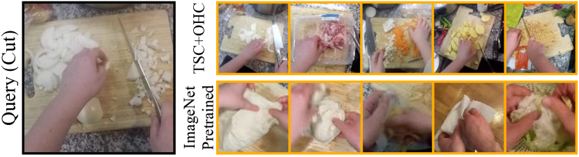
Figure 5: Object in similar states. Nearest neighbors in our learned feature space exhibit similar state.

Results. Table 1 reports the mean average precision (higher is better) for object state classification on the epic-states test set. We also report the standard deviation across 3 pre-training runs. We compare among our models and against a) ImageNet pre-training (i.e. no further self-supervised pre-training), b) non-temporal self-supervision via SimCLR [6], c) an alternate temporal self-supervision method (Time Contrastive Networks, TCN [53]), and d) semantic supervision from action classification on epic-kitchens and state classification on MIT States dataset [24]. We describe these comparison points as we discuss our key takeaways.

Features from TSC and TSC+OHC are more state-sensitive than ImageNet features. ImageNet pre-trained features provide a strong baseline with an mAP of 83.1%. TSC and TSC+OHC boost performance to 84.2% and 84.8%, respectively. Improvements get amplified in the challenging low-data and novel category settings for all models, with our full model TSC+OHC improving upon ImageNet features by 4.4% and 9.5%, respectively. These trends are also borne out when we visualize nearest neighbors in the learned feature spaces in Figure 5.

TSC and TSC+OHC outperform other competing self-supervision schemes. Temporal SimCLR, even by itself, is more effective than vanilla SimCLR that has access to the same crops but ignores the temporal information. We also outperform TCN [53], a leading method for temporal self-supervision, and TCN combined with SimCLR. TCN uses negatives from the same track. These are harder to identify in epic-kitchens because of the large variability in time-scales at which changes occur (e.g. open vs. chop action).

Supervision from object-hand consistency improves performance. TSC+OHC improves over just TSC by 0.6% with larger gains (of up to 5.2%) in the more challenging novel category and limited data settings. This confirms our hypothesis that observation of what hands are doing, aids the understanding of object states. Figure 6 shows some nearest neighbors retrievals that further support this.

TSC and TSC+OHC models outperform semantically supervised models. Conventional wisdom would have suggested pre-training a model on images gathered from the Internet for this or related tasks. MIT States dataset from Isola et al. [24] is the largest such dataset with 32,915 training images labeled with applicable adjectives. Surprisingly, our self-supervised models outperform features learned through supervised training on this dataset by 3.3 to 9.6%, perhaps due to the domain gap between Internet and egocentric data.

Another common belief is to equate action classification to video understanding. We assess this by comparing against features from the action classification task on epic-kitchens. This model was trained on our tracks using the most common 32 action labels along with their temporal extent, available as part of the epic-kitchens dataset. Both TSC and TSC+OHC features outperform action classification features by 3 to 10%. Thus, while the action classification task is useful for many applications, it fails to learn good state-sensitive features.

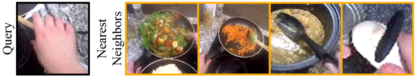
Figure 6: Objects affording similar hands. We retrieve objects that are associated with hands having features similar to the query hand. Objects that are being interacted with similarly get retrieved.

Ablations. In Supplementary, we compare alternate ways of obtaining tracks when learning with TSC. We ablate two aspects: what we track (background crop, background object, object-of-interaction) and how we track it (no tracking, off-the-shelf tracker [35], hand-context). Ablations reveal the utility of object-of-interaction tracks particularly as they enable use of hand consistency. We also study the role of appearance and motion individually for representing the hand. We found both to be useful over TSC with motion being more important than appearance.

4.2 Regions of Interaction

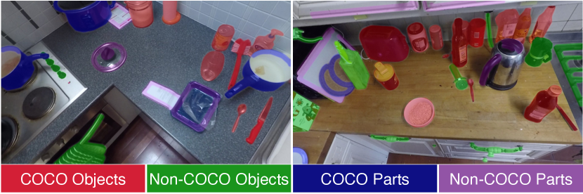
Figure 7: Images from the proposed epic-roi dataset. Each image is annotated for regions of interaction i.e. where the human participants frequently interact with. Every annotation is also labeled with one of four attributes: COCO objects, Non-COCO objects, COCO parts, or Non-COCO parts.

Regions-of-Interaction Task and Dataset. We design and collect epic-roi, a labeled region-of-interaction dataset. epic-roi builds on top of the epic-kitchens dataset, and consists of 103 diverse images with pixel-level annotations for regions where human hands frequently touch in everyday interaction. Specifically, image regions that afford any of the most frequent actions: take, open, close, press, dry, turn, peel are considered as positives. We manually watched video for multiple participants to define a) object categories, and b) specific regions within each category where participants interacted while conducting any of the 7 selected actions. These 103 images were sampled from across 9 different kitchens (7 to 15 images with minimal overlap, from each kitchen). epic-roi is only used for evaluation, and contains 32 val images and 71 test images. Images from the same kitchen are in the same split. The Regions-of-Interaction task is to score each pixel in the image with the probability of a hand interacting with it. Performance is measured using average precision.

To enable detailed analysis, each annotated region is assigned two binary attributes: a) Is-COCO-object (if region is on an object that is included in the COCO dataset), b) Is-whole-object (if region covers the whole object). This results in 4 sub-classes (see Figure 7), allowing evaluation on more challenging aspects: e.g. small objects that are not typically represented in object detection datasets such as knobs (Non-COCO Object), or when interaction is localized to a specific object part such as the pan-handle (COCO Part) or the cutting-board-edges (Non-COCO Part). We also evaluate in the 1% slack setting where regions within 20 pixels (1% of image width) of the segmentation boundaries is ignored to discount small leakage in predictions.

Table 2: Average Precision for Region-of-Interaction Prediction. We report the overall AP and AP across the different types of interaction regions. We also report AP with 1% slack at the boundaries where we don’t penalize any leakage at regions within 20 pixels (1% of image width) of the mask boundaries. Without training on segmentation masks, our method outperforms methods based on objectness (SalGAN and DeepGaze2), action classification (Interaction Hotspots), and are able to come close to Mask RCNN that is trained with supervised segmentation masks. We achieve the strongest performance across all categories when combined with Mask RCNN. Highest numbers are boldfaced and the second highest are italicized.

	Overall		COCO Objects		Non-COCO Objects		COCO Parts		Non-COCO Parts
Slack at segment boundaries	0%	1%	0%	1%	0%	1%	0%	1%	0%	1%
Mask RCNN [all]	41.9	46.7	40.6	45.0	13.3	16.0	11.5	14.4	3.6	4.3
Mask RCNN [relevant]	64.0	70.0	72.2	78.1	22.8	28.7	31.0	39.6	6.8	9.1
Interaction Hotspots [42]	43.8	52.0	26.5	33.9	23.0	29.5	12.2	16.7	6.9	9.6
SalGAN [46]	48.7	56.4	40.8	49.1	24.5	31.0	11.4	15.7	4.7	6.4
DeepGaze2 [30]	55.7	64.6	44.8	55.1	35.8	45.4	11.4	16.5	7.4	10.8
ACP (Ours)	57.4	67.3	49.6	60.8	33.7	44.7	14.7	22.5	7.2	11.3
Mask RCNN+DeepGaze2	66.6	72.9	74.4	80.1	26.2	33.5	31.7	40.6	7.1	9.8
Mask RCNN+ACP (Ours)	68.7	76.4	76.2	83.0	31.1	41.9	32.5	43.7	7.4	11.4

Implementation Details. We train our model on 250 videos from the 2018 epic-kitchens dataset. We exclude videos from the 9 kitchens used for evaluation in epic-roi. Details of the grasp classification branch are in Section 4.3.

Results. Table 2 reports the average precision. We compare to three classes of methods: a) objectness based approaches SalGAN [46] and DeepGaze2 [30], trained using human gaze data / manual labels; b) instance segmentation based approaches that use Mask RCNN [22] predicted masks for all / relevant classes; and c) interaction hotspots from Nagarajan et al. [42] that derives supervision from manually annotated object bounding boxes and action labels in the epic-kitchens dataset. Given the strong performance of Mask RCNN-based methods, we also report the performance by aggregating predictions from Mask RCNN with ACP and next most competitive baseline, DeepGaze2. Aggregation is done using a weighted summation of predictions (weight selected using validation performance).

Overall, Mask-RCNN when restricted to relevant categories, performs the best. This is not surprising as it is supervised using over 1 million object segmentation masks. However, its performance suffers on non-COCO objects or their parts. Methods that utilize more general supervision start to do better. And in spite of not being trained on any segmentation masks at all, ACP (Ours) is able to outperform past methods. It starts to approach the performance of Mask RCNN, particularly in the 1% slack setting.

When combined with Mask RCNN, ACP achieves the strongest performance across all categories. It improves upon the Mask RCNN based method by 4.7%, indicating that our method is able to effectively learn about objects not typically included in detection datasets (e.g. stove knobs), and object parts (e.g. handle for fridges and drawers). Furthermore, our method provides a more complete interactive understanding by also predicting afforded grasps as we discuss in Section 4.3 and show in Figure 8.

Ablations. Experiments in Supplementary study the effects of variations in network input (not hiding hands, symmetric context, not filtering based on contact), model architecture, and data sampling and supervision (using just objects, or using just hands, or using hand masks rather than boxes). We find that all design choices contribute to ACP’s performance. Further improvements can be had from richer hand understanding (segmentation masks vs. box masks).

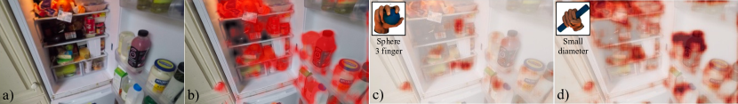
Figure 8: Object Affordance Predictions. For the input image (shown in (a)), we show the predicted regions of interaction in (b). Our method successfully detects multiple possible regions of interaction: bottles, jars, general objects in the fridge, and door knobs. We also visualize the per-pixel probability of affording the sphere 3 finger grasp in (c), and small diameter grasp in (d). The sphere 3 finger grasp is predicted for the door knob, bottle caps and cans; while the small diameter grasp is predicted for bottles, jars and cans. Thumbnails visualizing hand grasps reproduced from [15].

4.3 Hand Grasps Afforded by Objects

Grasps Afforded by Objects (GAO) Task and Dataset. We use the YCB-Affordance dataset [9] to evaluate performance at the Grasps Afforded by Objects (GAO) task. The dataset annotates objects in the scenes from [62] with all applicable grasps from a 33-class taxonomy [15]. We split the dataset into training (110K images, 776K grasps, used only to obtain a supervised ceiling), validation (60 images, 230 grasps) and testing (180 images, 760 grasps). Val and test sets contain novel objects not present in the training set. Given an image with a segmentation mask for the object under consideration, the GAO task is to predict the grasps afforded by the object. As multiple grasps are applicable to each object, we measure AP for each grasp independently and report mAP across the 7 (of 33) grasps present in the val and test sets.

Implementation Details. The grasp prediction branch in ACP is trained on predictions from a grasp classification model trained on the GUN71 dataset. We only use the 33 classes relevant to the task on the YCB-Affordance dataset from the 71-way output. To test our grasp affordance prediction on YCB-Affordance objects, we average the spatial grasp scores over the pixels belonging to the object mask.

We found it useful to adapt the GUN71 classifier to epic-kitchens to generate good supervision. This was done via self-supervision by using an additional $L_{\text{temporal}}$ loss on the epic-kitchens hand tracks (analogous to one used for objects in Section 3.1) while training on GUN71.

Results. For reference, chance performance is 30.2%, and supervised performance is 56.8%. The supervised method is trained on YCB-Affordance using ground truth annotations for afforded hand grasps on the 110K training images for the 15 training objects. Our method achieves an mAP of 38.1%. It reduces the gap between chance performance and the supervised method by 30%. Adaptation using $L_{\text{temporal}}$ on hands helped (34.3% vs. 38.1%).

5 Discussion and Limitations

We have shown that observation and analysis of human hands interacting with the environment is a rich source of information for learning about objects and how to interact with them; even when using a relatively crude understanding of the hand via 2D boxes. A richer understanding of hands (through segmentation, fine-grained 2D / 3D pose, and even 3D reconstruction) would enable a richer understanding of objects in the future. Our work relies on off-the-shelf models for generating data and supervision, and is limited by the quality of their output.

The ACP model in Section 3.2, doesn’t look at the pixels it is making predictions on. This causes our predictions to not be as well-localized. Our epic-roi task requires fine-grained reasoning for large objects (e.g. microwaves), but not as much for small objects because of subjectivity in annotation. Collecting fine-grained datasets for where we can interact with small objects in scenes will enable better evaluation. Similarly, large-scale in-the-wild datasets for evaluation of grasps afforded by objects can help. Finally, we tackled different aspects of interactive object understanding in isolation, a joint formulation could do better.

Ethical considerations, bias, and potential negative societal impact: Egocentric data is of sensitive nature. We relied on existing public data from epic-kitchens dataset (which obtained necessary consent and adopted best practices). Though, our self-supervised techniques mitigate bias introduced during annotation, we acknowledge that our models inherit and suffer from bias (e.g. what objects are present, their appearance and usage) present in the raw videos in epic-kitchens dataset. As with all AI research, we acknowledge potential for negative societal impact. Interactive object understanding can enable many useful applications (e.g. building assistive systems), but could also be used for large-scale automation which, if not thought carefully about, could have negative implications.

Acknowledgements: We thank David Forsyth, Anand Bhattad, and Shaowei Liu for useful discussion. We also thank Ashish Kumar and Aditya Prakash for feedback on the paper draft. This material is based upon work supported by NSF (IIS-2007035), DARPA (Machine Common Sense program), and an Amazon Research Award.

parttoc parttocHuman Hands as Probes for Interactive Object Understanding – Supplementary Material

S6 State Sensitive Feature Learning

S6.1 Model Details

S6.1.1 Baseline Models

We compare to six baseline models: ImageNet pre-trained model without any further training, three self-supervised models (SimCLR [6], TCN [53], and SimCLR+TCN), and two supervised models (action classification on epic-kitchens, and MIT States supervision). All models are initialized from ImageNet pre-training.

All models use the ResNet-18 backbone. We average pool the output after the second last layer to obtain a 512 dimensional representation. The self-supervised models use 3 projection layers with sizes 512, 512, 128. The 128-dimensional output from the last layer is used for computing the similarity. The semantically supervised models (i.e. those trained on MIT States dataset, or for action classification on the epic-kitchens dataset) only use a single linear classifier layer directly on top of ImageNet features. These additional layers were thrown out and just the ResNet-18 backbone is used for state classification experiment on epic-states. We only train a linear classifier on top of the learned ResNet-18 backbone for downstream state-classification on epic-kitchens dataset.

We use a batch size of 256 for pre-trainings. We optimize using Adam optimizer with a learning rate of $10^{-4}$. All models (with the exception of the two supervised baselines) are trained for 200 epochs and the last checkpoint is selected as the final model, which eliminates any dependencies on the pre-training validation set. All models are trained on a single NVidia GPU (RTX A40 or equivalent). We next list method specific hyper-parameters.

1. ImageNet Pre-trained Model. This model has no additional hyper-parameters.

2. SimCLR. We use the standard SimCLR augmentations in the following order: random resized crop with scale (0.5, 1.0), random horizontal flip, random color jitter with parameters (0.8, 0.8, 0.8, 0.2) and 80% probability, random grayscale with 20% probability, Gaussian blur with 12 size kernel and sigma set to (0.1, 2.0), and finally ImageNet normalization.

3. TCN. Let $w$ denote the length of the current track (number of frames). TCN’s window size is set to $\lfloor w/4\rfloor$ and the negative sample is guaranteed to be at least $\lceil w/2\rceil$ (negative window) away from the positive examples. Sampling the positive and negatives on opposite ends of the track ensures a large distance between them. TCN is optimized with a triplet margin loss. Let us reuse $o_{i},o_{i}^{\prime}$ as the positive pair and define $o_{i}^{\prime\prime}$ as the negative sample. Given an arbitrary margin $\alpha$ (in practice $\alpha=2$), the triplet margin loss is as follows. We chose the hyper-parameters as suggested by [53].

   $$||f_{o}(o_{i})-f_{o}(o_{i}^{\prime})||_{2}^{2}+\alpha<||f_{o}(o_{i})-f_{o}(o_{i}^{\prime\prime})||_{2}^{2}.$$ (1)

4. SimCLR+TCN. We combine SimCLR and TCN, by a) sampling negative from both within and across tracks, and b) using a NT-Xent loss from SimCLR [6]. We also adopt the image augmentations used in SimCLR.

5. Action Classification. We train ResNet-18 (initialized from ImageNet) on 32 action labels along with their temporal extent, available as part of the epic-kitchens dataset. These include: take, put, wash, open, close, insert, cut, pour, mix, turn-on, move, remove, turn-off, dry, throw, shake, squeeze, adjust, peel, scoop, empty, flip, fill, turn, check, spray, apply, pat, fold, scrape, sprinkle, break. The model samples two frames (in order) and uses them jointly to classify the action. This allows the model to disambiguate between open and close actions. The model is trained for 30 epochs and we select the model which performed the best on the action classification validation set. Validation performance peaked within 30 epochs.

6. MIT States. We train ResNet-18 (initialized from ImageNet) on the MIT-States attributes dataset [24]. The dataset consists of 115 classes and approximately 53K images. Examples of attributes include mossy, deflated, dirty, etc. This model is trained for 20 epochs and we select the model which performed the best on the MIT-States validation set. Validation performance peaked within 20 epochs.

S6.1.2 TSC and TSC+OHC Models

For TSC, object crops are selected by randomly sampling $o^{\prime}_{i}$ such that $o^{\prime}_{i}$ is no more than $\lfloor w/4\rfloor$ away from $o_{i}$ in the track, where $w$ is the length of the track.

For TSC+OHC, we use two separate models, one each for the object and the hand. The object model itself has 2 heads, one is used for the object-object similarity for $L_{\text{temporal}}$, and another for object-hand similarity for $L_{\text{hand}}$. The hand model only has one head. The hand model has additional layers to produce and combine the positional encodings that represent motion. The positional encoding is generated by alternating sines and cosines over 12 frequencies for each element of $h_{i}^{m}$. It is concatenated with the output of the ResNet-18 backbone. These combined features are projected to 512 dimensions with another linear layer and finally fed through the hand model’s loss head. Note that the object and hand crop fed through this model are not augmented with random horizontal flip to preserve handedness.

For the TSC+OHC model, tracks are independently sampled for computing the $L_{\text{temporal}}$ and $L_{\text{hand}}$ losses. Tracks with less than 4 frames of hands were filtered out to remove noise, which led to a pre-training dataset size of 53,661 tracks. The evaluation scheme remains the same as TSC since we only use the features learned by the object model. We throw out the hand model.

Loss Functions. Recall that $h^{a}_{i}$ and $h^{m}_{i}$ jointly represent the hand: $h^{a}_{i}$ describes the appearance and $h^{m}_{i}$ describes the motion. To detail $h^{m}_{i}$, consider the object bounding box for $o_{i}$ defined as $(o_{i,x1},o_{i,y1},o_{i,x2},o_{i,y2})$ where $(o_{i,x1},o_{i,y1}),(o_{i,x2},o_{i,y2})$ are the coordinates of the top left and bottom right corner of the bounding box, respectively. We define the hand crop bounding box similarly: $(h_{k,x1},h_{k,y1},h_{k,x2},h_{k,y2})$ where $k$ is uniformly sampled at random such that $|k-i|\leq 3$. $(*_{H},*_{W})$ represent the height and width of the bounding box and $(*_{xc},*_{yc})$ refer to the center coordinates of the bounding box. For an arbitrary $p$, we calculate $h^{m}_{i,p}$ and $h^{m}_{i}$ as follows:

$$h^{m}_{i,p} = \left[\frac{o_{i,xc}-h_{p,xc}}{o_{i,W}},\frac{o_{i,yc}-h_{p,yc}}{o_{i,H}},\frac{h_{p,W}}{o_{i,W}},\frac{h_{p,H}}{o_{i,H}}\right]$$ (2)

$$h^{m}_{i} = \left[h^{m}_{i,k-1},\quad h^{m}_{i,k},\quad h^{m}_{i,k+1}\right]$$ (3)

Assuming that all crops ($o_{i},o^{\prime}_{i},h^{a}_{i}$) are transformed using the standard SimCLR augmentations, we describe our application of normalized temperature scaled cross-entropy loss (NT-Xent) [6] below:

$$s^{oo^{\prime}}_{i,j} = \cdot{\operatorname{sim}(f_{o}(o_{i}),f_{o}(o^{\prime}_{j}))}$$ /1τ (4)

$$s^{oh}_{i,j} = \cdot{\operatorname{sim}(f_{h}(o_{i}),g_{h}(h_{j}))}$$ /1τ (5)

$$s^{hh}_{i,j} = \cdot{\operatorname{sim}(g_{h}(h_{i}),g_{h}(h_{j}))}$$ /1τ (6)

where $\operatorname{sim}$ refers to the cosine similarity, and $\tau$ is the temperature parameter (in practice $\tau=0.1$). Then $L_{\text{temporal}}$ and $L_{\text{hand}}$ losses are computed using $s^{oh}$, $s^{hh}$, $s^{oo}$ as follows:

$$L_{\text{temporal}} = -\sum_{i}{\left(\log\dfrac{\exp(s^{oo^{\prime}}_{i,i})}{\sum_{j:j\neq i}\exp(s^{oo}_{i,j})+\sum_{k}\exp(s^{oo^{\prime}}_{i,k})}\right)}-\sum_{i}{\left(\log\dfrac{\exp(s^{oo^{\prime}}_{i,i})}{\sum_{j:j\neq i}\exp(s^{o^{\prime}o^{\prime}}_{i,j})+\sum_{k}\exp(s^{oo^{\prime}}_{k,i})}\right)}$$ (7)

$$L_{\text{hand}} = -\sum_{i}{\left(\log\dfrac{\exp(s^{oh}_{i,i})}{\sum_{j:j\neq i}\exp(s^{oo}_{i,j})+\sum_{k}\exp(s^{oh}_{i,k})}\right)}-\sum_{i}{\left(\log\dfrac{\exp(s^{oh}_{i,i})}{\sum_{j:j\neq i}\exp(s^{hh}_{i,j})+\sum_{k}\exp(s^{oh}_{k,i})}\right)}.$$ (8)

S6.2 EPIC-STATES Dataset and State Classification Task

S6.2.1 Data Annotation

epic-states is collected on top of the ground-truth object-of-interaction tracks and corresponding object category labels from Damen et al. [10]. We filter out 13 object categories of interest: drawer, knife, spoon, cupboard, fridge, onion, fork, egg, potato, bottle, microwave/oven, carrot, and jar. We chose a maximum of 5 frames from each track. These object crops are then annotated for states individually for each object category.

We used a commercial service to obtain annotations for our dataset. Each image was annotated once and then reviewed by a high-quality annotator (determined using the accuracy on the task). We also included an ambiguous class and reject images with the ambiguous label, resulting in 14,346 annotated images.

Annotation Instruction. We gave the annotators the following instructions:

Given an image, choose all applicable categories/states from the ones available. If the image is considerably noisy or the object of specified category cannot be identified, annotate the image as ambiguous. When multiple objects are visible, annotate the most dominant object of the specified category. Note that images are captured in-the-wild and small motion blur, therefore, should not be considered as noise.

For each object category, we specify the set of states to consider, and any other object category specific instructions. Below we club the instructions for multiple objects, but note that images from different object categories were annotated separately.

1. Microwave/Oven, Cupboard, Drawer, and Fridge: The applicable states are open, close, and ambiguous. From open/close only one state would be applicable, i.e. a drawer can not be both, open and close at the same time.

2. Jar and Bottle: The applicable states are inhand, outofhand, open, close, and ambiguous. From inhand/outofhand, and open/close only one state would be applicable, i.e. a bottle can not be both, inhand and outofhand; or both, open and close.

3. Onion and Potato: The applicable states are inhand, outofhand, raw, cooked, whole, cut, peeled, unpeeled, and ambiguous. From inhand/outofhand, raw / cooked, peeled / unpeeled, and whole / cut only one state would be applicable. For green onions, we asked the annotators to not label the peeled/unpeeled attribute.

4. Carrot: The applicable states are inhand, outofhand, raw, cooked, whole, cut, and ambiguous. From inhand/outofhand, raw/cooked, and whole/cut only one state would be applicable.

5. Spoon, Fork, and Knife: The applicable states are inhand, outofhand, and ambiguous. From inhand/outofhand, only one state would be applicable.

6. Egg: The applicable states are inhand, outofhand, raw, cooked, and ambiguous. From inhand/outofhand, raw/cooked, only one state would be applicable.

S6.2.2 Dataset Statistics

Splits. We split the dataset into train, val and test splits based on participants. See participant assignment to the different splits in Table S3. Participants were assigned between val and test by minimizing the difference in joint object state (fridge-open, onion-cut, etc.) distribution between the sets. This ensures a good split of both objects and states.

Novel Object Categories. We list object categories that were used for training and testing for the novel object category experiment in Table S4.

Table S3: EPIC-STATES participants in each data split.

Split	Participants
Train	P01, P03, P06, P08, P13, P17, P21, P25, P26, P29
Validation	P04, P05, P07, P14, P22, P23, P27
Test	P02, P10, P12, P15, P16, P19, P20, P24, P28, P30, P31

Table S4: Novel Category Experiment. For the novel category experiment, we limited the training to objects in the first row, and evaluated on categories in the second row.

Train Objects	fridge, knife, drawer, potato, carrot, jar, egg
Novel Objects	spoon, cupboard, onion, fork, microwave / oven, bottle

Object and State Distributions. Table S6 and Table S5 shows the distribution of states and objects in epic-states, respectively. We also show the joint distribution of objects and states in Table S7 across the entire dataset. As noted, many different states are applicable to the same object.

Table S5: Objects in epic-states. For each objects in epic-states, we list the applicable states and how many instances we have for that object in each split.

Object	Applicable States	Train	Val	Test	Total
fridge	open, close	779	448	732	1959
spoon	inhand, outofhand	751	482	717	1950
knife	inhand, outofhand	749	551	729	2029
cupboard	open, close	683	449	429	1561
drawer	open, close	681	666	446	1793
onion	inhand, outofhand, raw, cooked, whole, cut, peeled, unpeeled	487	337	474	1298
fork	inhand, outofhand	353	206	259	818
microwave/oven	open, close	306	118	179	603
bottle	open, close, inhand, outofhand	294	179	257	730
potato	inhand, outofhand, raw, cooked, whole, cut, peeled, unpeeled	164	192	182	538
carrot	inhand, outofhand, raw, whole, cut	97	114	196	407
jar	open, close, inhand, outofhand	54	99	89	242
egg	inhand, outofhand,raw, cooked	32	199	187	418

Table S6: States in epic-states. For each state in epic-states, we list the object categories it is applicable to, and how many instances we have for that state in each split.

State	Applicable Objects	Train	Val	Test	Total
inhand	bottle, carrot, egg, fork, jar, knife, onion, potato, spoon	1861	1236	1699	4796
open	bottle, jar, cupboard, drawer, fridge, microwave / oven	2099	1440	1459	4998
outofhand	bottle, carrot, egg, fork, jar, knife, onion, potato, spoon	1280	1112	1227	3619
raw	carrot, egg, onion, potato	623	561	783	1967
close	bottle, jar, cupboard, drawer, fridge, microwave / oven	686	496	633	1815
cut	carrot, onion, potato	477	459	499	1435
peeled	onion, potato	450	423	465	1338
whole	carrot, onion, potato	270	178	351	799
cooked	egg, onion, potato	152	273	245	670
unpeeled	onion, potato	197	104	186	487

S6.2.3 State Classification Task

We construct binary state classification tasks by considering all non-ambiguous crops from object categories that afford the particular state label, as noted in Table S6. We throw out images that were ambiguous overall for all categories, or were ambiguous for the specific state category under consideration.

Table S7: Joint object and state distribution for epic-states. Note that multiple states are applicable to objects.

	open	close	inhand	outofhand	raw	cooked	whole	cut	peeled	unpeeled
bottle	286	358	521	205	✗	✗	✗	✗	✗	✗
carrot	✗	✗	223	184	399	✗	272	132	✗	✗
egg	✗	✗	118	300	210	204	✗	✗	✗	✗
fork	✗	✗	525	293	✗	✗	✗	✗	✗	✗
jar	136	103	154	78	✗	✗	✗	✗	✗	✗
knife	✗	✗	1331	699	✗	✗	✗	✗	✗	✗
onion	✗	✗	411	887	1000	296	290	1005	992	303
potato	✗	✗	236	300	358	170	237	294	346	184
spoon	✗	✗	1277	673	✗	✗	✗	✗	✗	✗
cupboard	1262	310	✗	✗	✗	✗	✗	✗	✗	✗
drawer	1479	315	✗	✗	✗	✗	✗	✗	✗	✗
fridge	1505	456	✗	✗	✗	✗	✗	✗	✗	✗
microwave/oven	330	273	✗	✗	✗	✗	✗	✗	✗	✗

open					close
peeled					unpeeled
raw					cooked
whole					cut
inhand					outofhand

Figure S9: Image samples corresponding to the different states in the epic-states dataset.

S6.3 Detailed Results and Ablations

S6.3.1 State-wise Performance

State-wise performance of considered methods for state classification is shown in Table S8. In particular, we see that ResNet-18 without any feature learning on our tracks already performs well on the open, raw, cooked, peeled, and cut categories for most settings. Nonetheless, our methods improve performance across the board. TSC+OHC improves upon TSC on all but one category in the challenging setting of novel categories with limited data.

Table S8: State-wise performance of models on epic-states test set in the different settings: novel objects with 12.5% training data, novel objects with 100% training data, all objects with 12.5% training data, and all objects with 100% training data.

Novel Objects [12.5%]	open	close	inhand	outofhand	raw	cooked	whole	cut	peeled	unpeeled	Mean
ImageNet Pre-trained	71.9 $\pm$0.0	53.5 $\pm$0.0	76.5 $\pm$0.0	62.8 $\pm$0.0	97.6 $\pm$0.0	87.1 $\pm$0.0	46.6 $\pm$0.0	82.1 $\pm$0.0	78.1 $\pm$0.0	45.9 $\pm$0.0	70.2 $\pm$0.0
TCN [53]	67.4 $\pm$4.6	50.9 $\pm$5.2	63.9 $\pm$2.5	46.7 $\pm$2.4	75.8 $\pm$1.3	32.9 $\pm$1.6	36.6 $\pm$2.6	76.6 $\pm$0.8	72.7 $\pm$1.7	37.3 $\pm$0.9	56.1 $\pm$1.9
SimCLR [6]	77.4 $\pm$2.8	61.7 $\pm$2.6	72.0 $\pm$1.1	53.6 $\pm$1.4	96.0 $\pm$1.0	84.6 $\pm$2.0	55.2 $\pm$5.2	82.3 $\pm$3.3	81.7 $\pm$1.0	54.2 $\pm$3.0	71.9 $\pm$0.2
SimCLR+TCN	73.7 $\pm$2.3	57.2 $\pm$2.8	68.9 $\pm$1.1	51.8 $\pm$2.5	90.5 $\pm$0.7	65.3 $\pm$1.3	42.2 $\pm$2.3	76.0 $\pm$1.9	72.9 $\pm$3.7	38.5 $\pm$3.7	63.7 $\pm$0.3
Semantic supervision
via EPIC action classification	76.0 $\pm$2.1	57.7 $\pm$1.5	76.4 $\pm$0.4	64.0 $\pm$1.4	95.3 $\pm$2.5	73.6 $\pm$9.0	56.3 $\pm$4.7	81.6 $\pm$2.0	79.4 $\pm$3.3	48.6 $\pm$4.2	70.9 $\pm$2.0
via MIT States dataset [24]	75.0 $\pm$0.9	56.2 $\pm$4.3	73.7 $\pm$0.8	60.4 $\pm$2.6	94.5 $\pm$2.7	77.5 $\pm$9.1	51.4 $\pm$1.3	87.1 $\pm$1.6	78.1 $\pm$2.8	46.8 $\pm$1.5	70.1 $\pm$1.5
Ours [TSC]	79.5 $\pm$1.1	63.5 $\pm$3.0	74.8 $\pm$1.9	54.5 $\pm$2.5	96.8 $\pm$1.3	81.7 $\pm$7.7	64.2 $\pm$3.3	87.0 $\pm$1.9	83.9 $\pm$1.6	58.8 $\pm$3.2	74.5 $\pm$1.0
Ours [TSC+OHC]	81.1 $\pm$0.5	62.5 $\pm$1.1	82.9 $\pm$0.9	67.5 $\pm$1.6	98.3 $\pm$0.6	88.1 $\pm$4.6	67.1 $\pm$2.6	90.4 $\pm$1.4	89.1 $\pm$1.8	70.4 $\pm$2.1	79.8 $\pm$0.6

Novel Objects [100%]	open	close	inhand	outofhand	raw	cooked	whole	cut	peeled	unpeeled	Mean
ImageNet Pre-trained	74.8 $\pm$0.0	57.6 $\pm$0.0	78.5 $\pm$0.0	70.3 $\pm$0.0	98.6 $\pm$0.0	92.0 $\pm$0.0	62.1 $\pm$0.0	91.4 $\pm$0.0	74.5 $\pm$0.0	45.4 $\pm$0.0	74.5 $\pm$0.0
TCN [53]	70.2 $\pm$3.9	52.6 $\pm$3.3	71.0 $\pm$1.6	53.5 $\pm$1.8	87.0 $\pm$3.9	49.9 $\pm$10.6	50.6 $\pm$3.5	84.6 $\pm$1.9	73.6 $\pm$3.5	45.6 $\pm$4.6	63.9 $\pm$1.1
SimCLR [6]	77.9 $\pm$2.2	62.2 $\pm$1.9	77.4 $\pm$1.3	63.1 $\pm$1.1	97.4 $\pm$1.3	94.0 $\pm$3.4	65.4 $\pm$4.3	90.3 $\pm$0.5	82.0 $\pm$0.5	61.6 $\pm$3.9	77.1 $\pm$1.0
SimCLR+TCN	76.1 $\pm$2.8	61.0 $\pm$2.9	75.2 $\pm$0.7	60.3 $\pm$2.0	92.7 $\pm$0.7	77.6 $\pm$5.9	52.5 $\pm$4.0	82.9 $\pm$2.8	69.6 $\pm$3.0	35.7 $\pm$5.2	68.4 $\pm$1.6
Semantic supervision
via EPIC action classification	80.0 $\pm$2.4	59.8 $\pm$3.1	82.4 $\pm$1.4	73.6 $\pm$1.0	97.1 $\pm$0.3	83.8 $\pm$8.2	59.6 $\pm$4.5	87.7 $\pm$2.1	84.6 $\pm$2.4	62.0 $\pm$7.9	77.0 $\pm$0.9
via MIT States dataset [24]	77.2 $\pm$1.7	58.3 $\pm$4.4	78.8 $\pm$2.1	67.9 $\pm$0.9	95.6 $\pm$2.4	85.6 $\pm$6.8	48.6 $\pm$2.2	89.2 $\pm$0.9	82.8 $\pm$4.5	54.9 $\pm$10.9	73.9 $\pm$0.7
Ours [TSC]	80.2 $\pm$1.2	63.8 $\pm$3.7	80.5 $\pm$1.6	63.5 $\pm$2.5	98.8 $\pm$0.4	94.1 $\pm$1.7	73.1 $\pm$1.6	93.1 $\pm$0.7	87.9 $\pm$0.2	67.2 $\pm$2.4	80.2 $\pm$0.4
Ours [TSC+OHC]	81.2 $\pm$0.4	63.2 $\pm$1.7	87.9 $\pm$0.7	77.3 $\pm$1.6	99.2 $\pm$0.4	94.7 $\pm$3.0	69.7 $\pm$3.3	92.9 $\pm$0.8	87.7 $\pm$1.6	64.5 $\pm$5.0	81.8 $\pm$0.4

All Objects [12.5%]	open	close	inhand	outofhand	raw	cooked	whole	cut	peeled	unpeeled	Mean
ImageNet Pre-trained	90.1 $\pm$0.0	62.3 $\pm$0.0	83.1 $\pm$0.0	73.4 $\pm$0.0	97.4 $\pm$0.0	83.8 $\pm$0.0	68.7 $\pm$0.0	85.1 $\pm$0.0	87.2 $\pm$0.0	51.2 $\pm$0.0	78.2 $\pm$0.0
TCN [53]	83.0 $\pm$1.7	48.6 $\pm$2.2	73.9 $\pm$2.1	55.9 $\pm$2.2	85.0 $\pm$0.8	40.4 $\pm$1.4	53.0 $\pm$2.2	72.7 $\pm$1.3	78.6 $\pm$0.3	33.6 $\pm$1.7	62.5 $\pm$0.8
SimCLR [6]	91.0 $\pm$0.8	65.3 $\pm$1.5	79.5 $\pm$0.9	64.6 $\pm$2.2	97.1 $\pm$0.6	82.0 $\pm$3.7	70.0 $\pm$1.8	82.1 $\pm$1.6	85.8 $\pm$2.3	57.2 $\pm$0.5	77.4 $\pm$1.0
SimCLR+TCN	87.9 $\pm$1.2	59.7 $\pm$1.6	76.8 $\pm$0.4	60.7 $\pm$2.2	95.4 $\pm$0.7	76.1 $\pm$4.9	63.3 $\pm$1.8	80.3 $\pm$0.6	82.3 $\pm$3.5	46.3 $\pm$3.5	72.9 $\pm$1.3
Semantic supervision
via EPIC action classification	88.5 $\pm$1.1	55.0 $\pm$1.6	83.1 $\pm$0.9	72.2 $\pm$0.2	95.9 $\pm$0.7	68.8 $\pm$3.7	60.0 $\pm$1.8	73.4 $\pm$2.2	79.7 $\pm$3.3	44.5 $\pm$1.5	72.1 $\pm$0.8
via MIT States dataset [24]	89.9 $\pm$0.1	58.5 $\pm$1.6	81.1 $\pm$1.2	70.0 $\pm$3.1	96.3 $\pm$1.2	78.9 $\pm$3.3	66.5 $\pm$2.0	86.3 $\pm$1.3	86.6 $\pm$1.3	50.4 $\pm$3.9	76.4 $\pm$0.6
Ours [TSC]	91.9 $\pm$0.5	65.6 $\pm$1.0	83.6 $\pm$0.6	69.8 $\pm$2.3	98.2 $\pm$0.0	86.7 $\pm$2.6	74.3 $\pm$2.7	88.3 $\pm$1.5	90.3 $\pm$0.1	65.2 $\pm$0.6	81.4 $\pm$1.0
Ours [TSC+OHC]	91.9 $\pm$0.6	63.5 $\pm$1.6	88.7 $\pm$0.4	77.9 $\pm$0.2	98.2 $\pm$0.1	88.5 $\pm$1.1	73.5 $\pm$0.9	89.5 $\pm$0.7	89.8 $\pm$0.6	64.8 $\pm$2.2	82.6 $\pm$0.2

All Objects [100%]	open	close	inhand	outofhand	raw	cooked	whole	cut	peeled	unpeeled	Mean
ImageNet Pre-trained	92.9 $\pm$0.0	68.3 $\pm$0.0	85.3 $\pm$0.0	78.2 $\pm$0.0	98.3 $\pm$0.0	88.5 $\pm$0.0	73.0 $\pm$0.0	89.4 $\pm$0.0	91.4 $\pm$0.0	65.1 $\pm$0.0	83.1 $\pm$0.0
TCN [53]	87.0 $\pm$1.0	56.7 $\pm$0.6	80.6 $\pm$1.0	67.2 $\pm$0.8	94.2 $\pm$0.9	68.5 $\pm$2.3	65.8 $\pm$2.3	82.7 $\pm$1.5	85.1 $\pm$1.5	46.4 $\pm$4.7	73.4 $\pm$1.4
SimCLR [6]	92.1 $\pm$0.8	67.6 $\pm$2.3	82.9 $\pm$0.5	71.3 $\pm$1.2	97.8 $\pm$0.6	86.0 $\pm$3.1	72.8 $\pm$1.6	86.9 $\pm$0.8	88.9 $\pm$2.2	64.1 $\pm$3.0	81.0 $\pm$0.9
SimCLR+TCN	90.5 $\pm$1.2	65.5 $\pm$1.3	81.3 $\pm$0.3	69.1 $\pm$1.5	96.9 $\pm$0.9	78.3 $\pm$6.3	68.9 $\pm$3.1	84.2 $\pm$1.8	84.9 $\pm$2.6	54.2 $\pm$2.5	77.4 $\pm$1.2
Semantic supervision
via EPIC action classification	91.1 $\pm$0.7	63.2 $\pm$1.2	86.6 $\pm$0.7	79.2 $\pm$1.3	97.0 $\pm$0.3	73.4 $\pm$4.4	65.2 $\pm$1.4	80.9 $\pm$1.3	87.1 $\pm$1.7	56.0 $\pm$9.9	77.9 $\pm$1.3
via MIT States dataset [24]	92.0 $\pm$0.1	66.9 $\pm$1.7	83.3 $\pm$0.5	73.9 $\pm$1.3	96.7 $\pm$1.8	82.5 $\pm$4.6	75.6 $\pm$2.3	89.3 $\pm$1.3	90.3 $\pm$1.7	64.4 $\pm$7.8	81.5 $\pm$1.3
Ours [TSC]	93.0 $\pm$0.3	69.6 $\pm$2.1	86.9 $\pm$0.6	75.8 $\pm$2.1	98.6 $\pm$0.1	89.0 $\pm$2.5	77.5 $\pm$2.6	89.8 $\pm$1.5	92.1 $\pm$0.6	69.3 $\pm$4.2	84.2 $\pm$1.0
Ours [TSC+OHC]	92.4 $\pm$0.8	66.1 $\pm$2.5	90.5 $\pm$0.5	83.1 $\pm$1.4	98.5 $\pm$0.1	91.1 $\pm$0.8	76.3 $\pm$2.9	91.2 $\pm$1.1	92.5 $\pm$1.1	66.7 $\pm$4.1	84.8 $\pm$0.4

S6.3.2 TSC+OHC Ablations

Table S9: We perform ablations on the components of TSC+OHC on the validation set. Both hand motion and appearance contribute to the performance over TSC, with motion being more important.

	Novel Objects		All Objects
Linear classifier training data	12.5%	100%	12.5%	100%
TSC	72.3 $\pm$1.3	77.8 $\pm$0.4	78.3 $\pm$0.3	81.2 $\pm$0.3
TSC+OHC (appearance)	73.8 $\pm$0.8	77.3 $\pm$0.5	78.4 $\pm$0.5	82.5 $\pm$0.6
TSC+OHC (motion)	74.6 $\pm$1.6	78.7 $\pm$0.6	78.8 $\pm$0.4	82.4 $\pm$0.2
TSC+OHC (motion + appearance)	75.1 $\pm$0.4	78.2 $\pm$0.2	78.6 $\pm$0.2	81.7 $\pm$0.3

We analyse the individual contribution of hand motion ($h^{m}_{i}$) and hand appearance ($h^{a}_{i}$) towards the performance of TSC+OHC. Table S9 shows that both components, by themselves, improve upon just TSC. Motion information gives larger boosts than appearance information; and both together lead to the best performance in the challenging setting of novel categories with limited data.

S6.3.3 Track Ablations

Mining object-level tracks from in-the-wild videos presents two challenges: a) how to select a useful patch to track, and b) how to successfully track it in the given ego-centric video.

Egocentric videos showcase objects that are undergoing non-trivial transformations (deformations, state changes, occlusion by hands). Furthermore, use of hand context could aid with tracking in egocentric videos that have large amounts of egomotion. We test the extent to which these advantages of working with egocentric videos contributes to performance. We generate several sets of tracks that ablate the two aforementioned factors. Visualizations for these tracks are shown by Figure S10, and the quantitative results are presented in Table S10.

Source for Starting Patches. We experiment with the following sources for the starting patch.

1. Object-agnostic Starting Patch. Here, we consider an arbitrary starting patch source, either a random crop or center crop in a frame. Random crops vary in scale and location, while the center crop is always a 256 $\times$ 256 crop from the $456\times 256$ image.

2. Starting Patch on Background Object. We detect background objects (i.e. not overlapping with objects of interaction as detected by the model from [55]) using Mask RCNN [22] with a ResNet101-FPN backbone trained on MS-COCO 2017 instance segmentation dataset. We only detections for categories commonly found in kitchens and remove classes like car, train, etc. We only consider the 10 highest scoring detections, and sample a detection that doesn’t overlap with the object-of-interaction as the starting patch.

3. Starting Patch on Object-of-Interaction (Ours). We use the object-of-interaction detections from Shan et al. [55]. As noted in the main paper, we use leave one out predictions from [55]: we split the train set into 5 parts by participants, retrain [55] on 4, use predictions on the 5^th (i.e. unseen participants); and repeat this 5 times over.

4. Ground Truth Objects-of-Interaction (Ceiling). For reference, we also report performance on using ground truth objects of interaction as annotated in the epic-kitchens dataset. We use these with ground truth tracking (see below).

Tracking Algorithm. We experiment with the following tracking algorithms.

1. No Tracking. Here, we don’t do any tracking and copy over the box from the previous frame, to the same location in the current frame.

2. Off-the-Shelf Tracker. We use SiamRPN++ tracker from [35] to track the object from one frame to the next. Given a starting crop, the tracker produces bounding boxes for crop in consecutive frames. In practice, we only consider a tracker-produced bounding box to be valid if it has a score above 0.1. We allow for up to two frames of either missing or invalid detections, or a max of 256 frames tracked, before sub-sampling and saving the track.

3. Hand-context (Ours). To construct our tracks, we focus on objects-of-interaction detected by [55] along with information about what hands do they correspond to. We do this jointly with the object-of-interaction starting patches described above. In more detail, we utilize hand-object detections for both, finding the starting patch and tracking it. Specifically, we start with a frame and find all interacted objects with a score above 0.2 and start tracking them independently. At the next frame, we receive another set of valid objects bounding boxes and try to match them with the previous frame’s detections by posing the problem as a linear sum assignment in a bipartite graph where the cost is the intersection over union (IoU) over the two bounding boxes (provided that IoU $>$ 0.4). Boxes still not matched with previous boxes start their own track. Tracks also have an 8 frame buffer with no matches before they are closed. We subsample the tracks to 10fps. We cap the track length at 25.6s, and split longer tracks. We get a total of 61.3K tracks.

4. Ground Truth (Ceiling). Here we use the ground truth object-of-interaction tracks provided in the epic-kitchens dataset (used in conjunction with ground truth object-of-interaction above). We use the bounding box annotations for the object-of-interaction from Damen et al. [10] on epic-kitchens dataset. Since these annotations are provided at 0.5 fps, we interpolate the bounding box for the intermediate frames to get dense tracks. This gives us 16,474 tracks with an average length of 66 frames.

Table S10: Comparison on validation set for various tracking approaches used for learning state sensitive features with Temporal SimCLR. Tracks obtained with the hand-object-interaction detector perform the best and come close to hand annotated tracks [10] in performance. Italicized rows correspond to our proposal in this paper.

Starting Patch Source	Tracking Algorithm	TSC Val mAP
Center crop	None	72.9
Random crop	None	77.1
Object-of-interaction [55]	None	79.2
Random Background Crop	SiamRPN++ [35]	77.6
Random Background Object	SiamRPN++ [35]	80.6
Object-of-interaction [55]	SiamRPN++ [35]	79.7
Object-of-interaction [55]	Hand context	81.2
GT Object-of-interaction	Ground Truth	83.5
Object-of-interaction [55]	Hand context	81.7 (TSC+OHC)

Results. Table S10 shows the performance of TSC on the various tracks. As noted in the main paper, use of object-of-interaction tracks offers two advantages: they stabilize for the large egomotion in egocentric videos, and focus on aspects of the scene that are undergoing interesting (non-viewpoint) transformations. No stabilization performs poorly. Stabilization using off-the-shelf tracker SiamRPN++ [35] also works well. However, tracking with hand context enables use of Object-Hand Consistency which aids performance. Ground truth tracks annotated in epic-kitchens dataset lead to better learning, indicating that better detection and tracking of objects-of-interaction can improve performance further.

Random+ No tracking
MaskRCNN+ SiamRPN++
InteractionObj+ HandContext [Ours]

Figure S10: Sample track from the random crop with no tracking (Random), the background object crop with MaskRCNN + tracking with SiamRPN++ (MaskRCNNN + SiamRPN++), and our tracks that use objects-of-interaction and track using hand context. We see that ego-motion in egocentric videos leads to large drift by the end without any tracking. We see that the background object tracks fail to capture meaningful appearance changes. For our tracks, we see the object in a variety of poses with distinct appearances.

S7 Object Affordance Prediction

S7.1 EPIC-ROI Dataset and Task

Task Definition. The ROI (Region of Interaction) task is to predict regions where human hands frequently touch in everyday interaction. Specifically, image regions that afford any of the most frequent actions: take, open, close, press, dry, turn, peel are considered as positive.

Data Sampling. We randomly sampled 500 images from 9 participants: P01, P08, P11, P02, P32, P18, P04, P09, P03. From these participants, we only use videos present in the test set of epic-kitchens dataset (2018 version). We annotated frames at 1920 $\times$ 1080 resolution. The images may or may not contain participant hands (if they were present, they were annotated and ignored during evaluation) . We manually filter out images to minimize motion blur, out of distribution frames (for example, completely dark frames at the starting of some videos or rare views such as picking a spoon that fell onto the floor). We made sure to minimize redundancy among frames by selecting the most diverse 7 – 15 frames from each participant.

Annotation Procedure. To determine where participants frequently interact in the scene, we manually watched the videos from these participants and created a list of objects that underwent interaction objects and also identified the interacted regions. Then, for every considered action, we annotated applicable regions of interaction using polygons for larger objects (such as bottles, jars etc.), and lines for thin regions (wires, rims and object edges). The lines for the rims and edges of objects were converted to regions by dilating them by 25 pixels to convert them to strips. Annotation for 10 images from 1 participant took 120 minutes on average. Lastly, we aggregate the annotations across all actions to generate the EPIC-ROI ground truth segmentation mask.

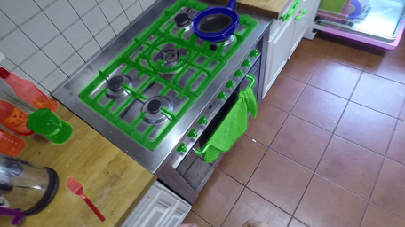
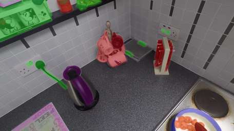
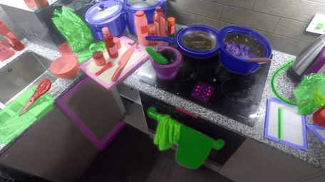
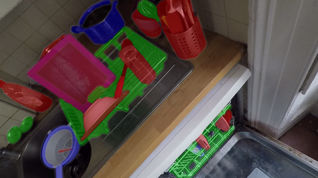
Figure S11: Annotated images from epic-roi dataset. We show some sample images from the dataset annotated for evaluating region of interaction predictions. Each annotated region is attributed with one of the four labels: COCO objects (red), Non-COCO objects (green), COCO parts (blue), and Non-COCO parts (magenta).

To enable detailed analysis, every annotation is also assigned one of the four labels: COCO objects, Non-COCO objects, COCO parts, and Non-COCO parts. To determine the set of COCO objects, we first select only the relevant classes removing categories like cat, dog, bird etc. This leaves us with the following categories: backpack, umbrella, handbag, tie, suitcase, sports ball, baseball bat, baseball glove, tennis racket, bottle, wine glass, cup, fork, knife, spoon, bowl, banana, apple, sandwich, orange, broccoli, carrot, hot dog, pizza, donut, cake, chair, mouse, remote, keyboard, cell phone, toaster, book, vase, scissors, hair drier, toothbrush, microwave, oven, sink, and refrigerator. We further observed that removing microwave, oven, sink, and refrigerator from the relevant categories improves the performance of Mask RCNN on the validation split (see Table S12). Thus, we don’t include objects from these 4 categories into COCO objects. Figure S11 shows some annotated images from our validation split where different categories (out of above four) are assigned different colors.

Table S11: Val and test sets for epic-roi dataset.

Split	Participants	# Frames
Validation	P03, P04, P09	32
Test	P01, P02, P08, P11, P18, P32	71

Dataset Splits. We split the collected dataset into validation and testing sets based on the participants. P03, P04, and P09 are in the validation set with a total of 32 frames. P01, P02, P08, P11, P18, and P32 are in the test set with a total of 71 images.

S7.2 Grasps Afforded by Objects (GAO) Task

Task Definition. The task is to predict the hand-grasps afforded by objects present in the scene where each object can afford multiple grasps. The task also requires reasoning about the occlusion between objects which can leave some of the hand-grasps inapplicable.

Datasets. We utilize YCB-Affordance dataset [9] that builds upon YCB-Videos [62] (sample frames shown in Figure S12) to set up GAO Task. The dataset annotates each object with the afforded hand grasps (see Figure S12 (right)).

For our methods and the baseline alike, we assume that objects have already been localized (we use the object masks provided with the dataset). This side-steps the detection problem and allows us to focus on the task of predicting afforded grasps. For the baselines, predictions are made on a crop around the object of interest. For our method, dense predictions from our model are aggregated over the segmentation mask to obtain the final classification (more below).

Splits. We divide the YCB-Affordance dataset into three parts for training, validation and testing. We make sure that the training, validation and test sets do not overlap in the objects. Further, there is no overlap in the videos from training, validation and test sets. This results in a training set consisting of 77 videos, validation set with 6 videos and testing set with 9 videos. We further only use 15 objects (out of 21) from the training set to train the supervised baseline. For validation and testing, we use the remaining 6 objects to compute the metrics. Since the scene is static, and the camera motion is slow, we sub-sample 60 frames (10 from each video) from the validation videos to create the validation set, and 180 frames (20 from each video) to create the testing set. We use all the frames (110K) from training videos to create the training set for supervised ceiling. The splits ensure that we test generalization to novel objects.

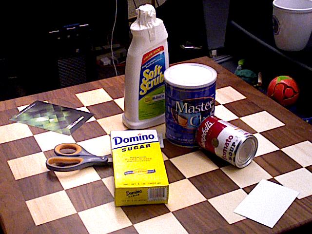
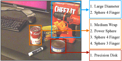
Figure S12: Sample frames from YCB-Videos [62]. We use annotations from Corona et al. [9] on the YCB-Videos [62] to setup the GAO task. The task is to predict the hand-grasps afforded by the objects present in the scene (see right figure). This requires reasoning about object shape and occlusion patterns that can render some grasps inapplicable.

S7.3 Model Details

S7.3.1 Affordances via Context Prediction (ACP) Details

Architecture. We use the ResNet-50 backbone as the encoder. The region of interaction branch uses a decoder that consists of 4 deconvolution layers with $4\times 4$ kernels and stride length of 2 and a padding of 1. Lastly, we have a $5\times 5$ average pooling layer with padding 2 and stride 1 which outputs the final ROI-prediction. The grasp prediction branch, uses one fully-connected layer followed by 33 binary classifiers on top of the output from the encoder.

Training Splits. We use participants P05, P06, P07, P10, P12, P13, P14, P15, P16, P17, P19, P20, P21, P22, P23, P24, P25, P26, P27, P28, P29, P30, P31 for training the model. Note that these are disjoint from the participants used for validation and testing in epic-roi, as listed in Table S11.

Data Sampling. For training our ACP model, we extract patches from $456\times 256$ epic-kitchens frames (2018 version). We use the hand and object-of-interaction detections to generate the ground-truth segmentation mask (by pasting the detections). We only use object-of-interaction detections that have a confidence score $\geq 0.8$, and that are smaller than 150 pixels in width and height. Next, we sample positives around the detected hands and detected objects-of-interaction. For hands, we randomly select a square patch 1 to 1.3 times the size of the detected hand box, centered at the hand (positive) or randomly located elsewhere in the image (negative). For sampling around the objects, we only consider object-of-interaction detections that have width and height greater than 20 pixels, and we sample a square patch inside the object-of-interaction box (positive). The width of the sampled patch is randomly varied between 0.5 to 0.75 times the size of the detected object-of-interaction box. We train on all participants except the ones in the epic-roi validation and testing sets. For training the grasp prediction branch, we only use the positive patches sample centered at the hand.

Patches are resized to $128\times 128$ for training. Note that the bottom center $64$ region is masked out before feeding into the networks both at train and test times.

Loss function. Our loss contains two terms $L_{\text{seg}}$ and $L_{\text{grasp}}$, the former training the region of interaction branch and the latter training the grasp prediction branch. Both losses encourage the network to focus on the surrounding context to make prediction about the hidden hand.

$L_{\text{seg}}$ computes the binary cross-entropy between the predicted segmentation mask and the ground truth segmentation mask (as derived by pasting detection boxes). We weight the positive pixels by a factor of 4.

$L_{\text{grasp}}$ is trained on predictions from a classifier trained on the GUN-71 dataset [51]. We only consider scores for the 33 hand grasps (that are annotated in YCB-Affordance dataset) from the GUN-71 classifier. We use the highest scoring class as the positive class. We create a set of negatives which consists of the least scoring $K=15$ classes. This generates both the positive and negative data for training the grasp prediction head.

$L_{\text{seg}}$ is trained on all positive and negative patches described above. $L_{\text{grasp}}$ is only trained on positive patches (i.e. those that are around the hands).

We train both the segmentation head and the grasp prediction branch jointly by combing the two loss functions as,

$$L=L_{seg}+0.5\cdot L_{grasp}.$$ (9)

Training Details. We use a batch size of 64 and Adam optimizer with a learning rate of $10^{-4}$. During training, we also perform horizontal flips, motion blur and color jitter augmentations on the input image. The masked context region is resized to $128\times 128$ before being input to the model. We train for a total of 400 epochs (each epoch consisting of 256 iterations on randomly sampled batches with batch size of 64) and then validate checkpoints at epoch 300, 350, and 400 to select the best model for evaluation. Training took 6 hours on a single modern GPU (RTX 2080 Ti or equivalent).

Supervision for Grasp Prediction Branch. Here, we provide more details about the GUN-71 classifier that is used to generate the necessary supervision for training ACP.

This GUN-71 classifier is trained on hands cropped from the GUN-71 dataset from Rogez et al. [51]. We use a hand detector [55] to crop out hands from the GUN-71 dataset resulting in 8403 crops for training (Subjects 1, 2, 3, 4, 5, and 6) and 1655 crops for validation (Subject 7). The classifier uses a ResNet-18 backbone with two fully connected layers (512 and 128 units), followed by a 71-way classification layer. This model is trained using hand grasp annotations in the GUN-71 dataset with a cross-entropy loss.

In addition to this grasp classification layer, we also have another head consisting of one linear layer (128-dimensional output) that is trained using $L_{\text{temporal}}$ on the epic-kitchens dataset to adapt the GUN-71 classifier to work well on epic-kitchens dataset. This $L_{\text{temporal}}$ uses the hand tracks obtained using detector from [55] on the epic-kitchens dataset, as used by the other parts of our paper.

This network is trained jointly by minimizing $L_{c}+L_{\text{temporal}}$ using Adam optimizer with a learning rate of $10^{-4}$ and 0.05 weight decay. We use a batch size 128. We perform random crops, horizontal flips, and color jitter as augmentations. We train for a maximum of 60 epochs where we early stop based on the validation performance. For $L_{\text{temporal}}$, we use a window of length 10 to sample positive hand crops. We only train on tracks with a minimum length of 15 frames. We save the model after every 3 epochs, and select the snapshot based on the validation performance on the GAO task. Typically, training for 24-30 epochs resulted in the best performance where each epoch consisted of training for 64 iterations.

ACP (no $L_{\text{temporal}}$). This model is trained similarly to ACP but only for minimizing $L_{c}$ cross entropy loss for classification.

Inference. At test time, we uniformly sample square context regions of size 60, 100, and 160 from $1920\times 1080$ images. We sample 4000 regions for each size, resulting in a total of 12000 regions. We resize the sampled patches to $128\times 128$ and mask out their bottom center $64\times 64$ region, before feeding them into our learned models to obtain the 12000 $64\times 64$ predictions.

These predictions are spatially aggregated, individually for both the afforded hand grasps and regions of interaction, by resizing and pasting at the corresponding locations. For GAO task, we only use the spatially aggregated grasp predictions, and for the ROI-prediction task, we only use the spatially aggregated ROI prediction. For evaluation on epic-roi, we also smooth our predictions using a Gaussian kernel (with standard deviation of 25) to suppress high frequencies. To generate affordances (for example in Figure 8), we simply multiply the two spatial predictions.

Inference on YCB-Affordance. We do inference over 800 $160\times 160$ patches to obtain pixel-wise grasp predictions for each of the 33-hand grasps. We then compute the average score within each object mask and use that to compute 33 scores, one each for each grasp type.

S7.3.2 Region of Interaction (RoI) Baselines

Mask RCNN. We use an FPN-based (Feature Pyramid Network) Mask RCNN model trained on MSCOCO with a ResNet-101 backbone for implementing this baseline. For inference, we predict 1000 detections per image with an NMS threshold of $0.7$. To get the RoI prediction, we multiply the class-score with the soft instance segmentation mask, and paste it at the corresponding detection locations.

Table S12: Selecting Relevant COCO Categories to Maximize Mask RCNN Performance. We observe that using predictions for microwave, oven, sink, refrigerator or all four, reduces the performance of Mask RCNN on validation set. This is because the region-of-interaction task requires localizing the regions of interaction on these objects and not segmenting them out as a whole. Consequently, we remove these 4 object classes from the relevant categories. We compare to this stronger Mask RCNN baseline.

	Overall AP
Slack at segment boundaries	0%	1%
Mask RCNN [relevant]	65.7	72.1
Mask RCNN [relevant] w/ oven	50.0	58.1
Mask RCNN [relevant] w/ microwave	61.7	73.1
Mask RCNN [relevant] w/ sink	54.4	60.7
Mask RCNN [relevant] w/ refrigerator	52.6	57.7
Mask RCNN [relevant] w/ oven, microwave, sink, refrigerator	47.3	53.3

Mask RCNN [relevant]. Before pasting the predicted segmentations, we filter out detections corresponding to the relevant categories. Specifically, we consider the following object categories that we selected so as to maximize the AP on the validation set (see ablation in Table S12): backpack, umbrella, handbag, tie, suitcase, sports ball, baseball bat, baseball glove, tennis racket, bottle, wine glass, cup, fork, knife, spoon, bowl, banana, apple, sandwich, orange, broccoli, carrot, hot dog, pizza, donut, cake, chair, mouse, remote, keyboard, cell phone, toaster, book, vase, scissors, hair drier, and toothbrush.

Interaction Hotspots. We use the pre-trained model (with a dilated ResNet-50 backbone) provided by Nagarajan et al. [42] to predict interaction hotspots on epic-roi. Specifically, we uniformly sample 800 patches of size $400\times 400$, resize to $224\times 224$ to feed into their model, get $28\times 28$ predictions from their model, upsample and paste these predictions at the corresponding location. We selected the ($400\times 400$) patch size based on the validation set performance. We did not observe any improvement in performance on increasing the number of patches sampled. Note that the model from [42] is a action-specific model. We convert their predictions into per-pixel interaction probability by taking the max score across actions at each pixel.

DeepGaze2. We use the predictions from DeepGaze2 [30] model to compute the AP on the RoI-prediction task.

SalGAN. We use the predictions from SalGAN [46] model to compute the AP on the RoI-prediction task.

Mask RCNN + X. We combine predictions, $P_{\text{X}}$ from models (DeepGaze2, Ours) with predictions $P_{\text{Mask~{}RCNN}}$ from Mask RCNN [relevant] to obtain combined predictions which are denoted as Mask RCNN + DeepGaze2 and Mask RCNN+ACP in the main paper. This is done by a pixel-wise combination with scalar weights:

$$P^{\text{comb}}_{X}=w\cdot P_{\text{Mask~{}RCNN}}+(1-w)\cdot P_{\text{X}}$$ (10)

We set $w$ to $2/3$ when combining with ACP, and to $1/2$ when combining with DeepGaze2. This scalar weight was obtained through validation on the validation set. We additionally found it useful to smooth the output from our model (Gaussian filtering with standard deviation of $25$ pixels, image size was $1920\times 1080$). Such blurring wasn’t useful for predictions from DeepGaze2.

S7.3.3 Grasps Afforded by Objects (GAO) Baselines

Chance. As chance performance, we report the fraction of positive data for each grasp in the dataset. This corresponds to a flat precision recall plot.
Supervised Ceiling. To train the supervised ceiling, we use the training split with 15 objects and 77 videos. We use a ResNet-50 backbone with a classifier head containing one fully-connected layer, followed by 33 binary classifiers. We train this network by sampling square patches centered at the object bounding boxes and use a binary cross entropy loss for training. We also use color jitter, horizontal flips and random crops on the sampled patches as data augmentation during training. We validate on the validation split on the held-out 6 objects.

S7.4 Detailed Results, Ablations, and Visualizations

S7.4.1 ACP Ablations

We study the effect of the different choices regarding supervision, data preparation and network input, and network architecture, made in the design of ACP. We conduct these experiments on the validation sets and report performance on the ROI task and the GAO task (where applicable). For the ROI task, we report the performance in isolation, and upon combination with Mask RCNN. Results are presented in Table S13.

Data preparation and network input. Our full model masks out the hand before feeding in patches to the network for training, and uses an asymmetrical context window around the masked region. Furthermore, we only make predictions for objects and hands when they are in contact with the hand. We ablate these choices, and find that all three of these choices contribute to the performance of the full ACP model.

Supervision and data sampling. Our full model uses the regions for both the hand and the object as target and for sampling data during training. We see a large drop in performance on the ROI task when not using the object regions for data sampling or as target (denoted as ‘no object’). Not using the hand regions for data sampling or as targets (denoted as ‘no hand’) leads to a small drop in performance for the ROI task but additionally renders it impossible to train for the GAO task. The role of hands is further emphasized when we switch to using hand segmentation masks rather than box masks (as used in all other experiments). Richer understanding of the hands leads to improved performance on the ROI task.

Network architecture. Our ACP model as used in the main paper takes in a $2s\times 2s$ input and produces a $s\times s$ output. We also experimented with a symmetric architecture ($2s\times 2s$ input and output). This can lead to better spatial alignment and ease learning. We report metrics with two such architectures, (i) where we put the loss on the bottom center patch, and (ii) where we put the loss in the entire output window. We observe slight improvements in performance from these architectural modifications.

Table S13: Variations of ACP. Average precision for Region-of-Interaction prediction and mean average precision for GAO task, each on the respective validation sets. For ROI prediction task, we report results using raw ACP predictions as well as when combined with Mask RCNN. We train each ablation three times and report the mean and the standard deviation ($\mu$$\pm$$\sigma$).

	ROI (Overall AP)		ROI (Overall AP) [+Mask RCNN]		GAO (mAP)
Methods	0% Slack	1% Slack	0% Slack	1% Slack
ACP (full model)	61.4 $\pm$0.3	73.3 $\pm$0.5	70.9 $\pm$0.1	79.5 $\pm$0.2	42.2 $\pm$2.6
Data preparation and network input
ACP (no hand hiding)	60.8 $\pm$0.3	72.4 $\pm$0.4	70.3 $\pm$0.1	78.8 $\pm$0.1	42.0 $\pm$5.2
ACP (no contact filtering)	59.9 $\pm$0.7	71.4 $\pm$0.8	70.5 $\pm$0.2	79.0 $\pm$0.3	43.0 $\pm$1.2
ACP (symmetric context)	60.2 $\pm$0.2	72.4 $\pm$0.2	70.0 $\pm$0.2	78.5 $\pm$0.1	39.1 $\pm$1.0
Supervision and data sampling
ACP (no object)	53.6 $\pm$1.0	65.1 $\pm$1.3	69.5 $\pm$0.2	77.3 $\pm$0.3	41.4 $\pm$5.9
ACP (no hand)	60.8 $\pm$0.8	72.8 $\pm$0.7	70.7 $\pm$0.3	79.3 $\pm$0.2	N/A
ACP (hand segmentation masks as opposed to box-masks)	62.1 $\pm$0.5	74.0 $\pm$0.4	71.1 $\pm$0.4	79.7 $\pm$0.4	42.5 $\pm$2.7
Network architecture
ACP ($2s\times 2s$ output, loss everywhere)	61.5 $\pm$0.4	73.7 $\pm$0.5	70.6 $\pm$0.2	79.2 $\pm$0.1	40.7 $\pm$2.6
ACP ($2s\times 2s$ output, loss on bottom center)	61.7 $\pm$0.3	73.4 $\pm$0.1	71.1 $\pm$0.2	79.7 $\pm$0.2	41.6 $\pm$5.0

S7.4.2 GAO Category-wise Performance

The test set only contains 7 (out of 33) grasps, we report the mean average precision over these 7 categories. The class-wise performance for ACP is shown in Table S14. We also report the chance performance along with a supervised ceiling.

Table S14: Class-wise performance on the GAO test set. We report average precision for each of the 7 hand grasp type contained in the test set. For ACP (no $L_{\text{temporal}}$) and ACP, we conducted the experiment three times and report the mean performance. We also report the standard deviation over three runs for ACP and ACP (no $L_{\text{temporal}}$).

Grasp Type	Chance	ACP (no $L_{\text{temporal}}$) [Ours]	ACP [Ours]	Supervised Ceiling
Large Diameter	55.6	56.3 $\pm$5.7	45.2 $\pm$3.6	80.2
Medium Wrap	27.8	26.6 $\pm$5.8	20.4 $\pm$1.5	67.2
Power Sphere	27.8	23.6 $\pm$0.7	36.0 $\pm$3.6	68.4
Precision Disk	22.2	15.1 $\pm$0.8	14.9 $\pm$1.5	94.7
Parallel Extension	11.1	11.0 $\pm$0.4	28.1 $\pm$5.6	14.8
Sphere 4 Finger	50.0	68.8 $\pm$6.9	64.6 $\pm$1.9	56.6
Sphere 3 Finger	16.7	39.3 $\pm$6.2	57.3 $\pm$0.2	15.4
Mean	30.2	34.3 $\pm$0.8	38.1 $\pm$0.2	56.8

S7.4.3 Qualitative Results

1. We provide additional visualizations for ROI predictions made by ACP on the validation split of epic-roi dataset (see Figure S13). We observe that our method can locate regions that afford interaction such as drawer handles, knobs and buttons which are not typically annotated in object segmentation datasets. We also see that predictions are localized to object regions that afford interaction e.g. edges of plates.

   

   

   

   

   

   

   

   

   

   

   

   

   

   

   

   

   

   

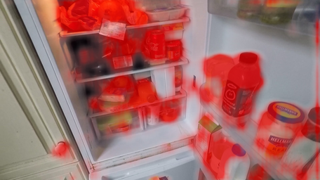
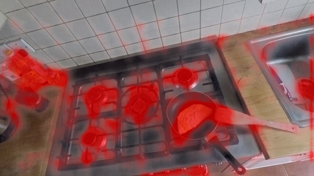
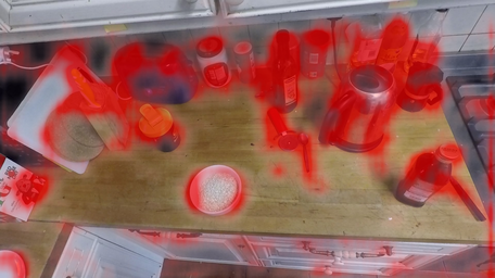
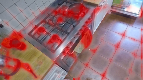
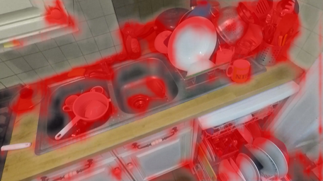
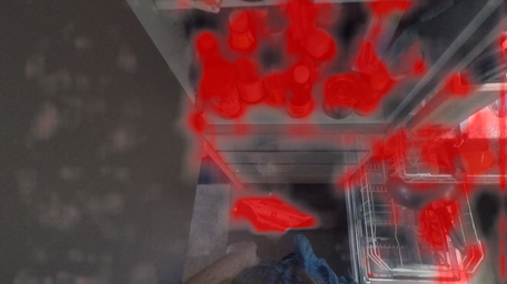
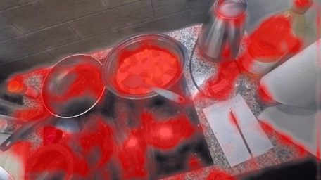
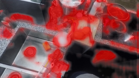
   Figure S13: Regions-of-Interaction (ROI) predictions on epic-roi dataset. We show ROI predictions on 18 images from the validation dataset. We observe that our method can locate regions that afford interaction: drawer handles, knobs and buttons (not typically annotated in object segmentation datasets). We also see that predictions are localized to object regions that afford interaction e.g. edges of plates.

2. We also visualize predictions for afforded grasps on the epic-kitchens dataset. We convert predicted grasp-specific heatmaps into detections (by finding scale-space blobs in the heatmaps) and visualize the top scoring detections across the validation dataset in Figure S14.

   Large Diameter
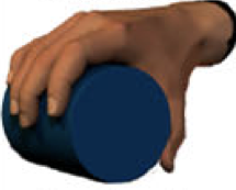
   Medium Wrap
   Power Sphere
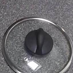
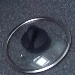
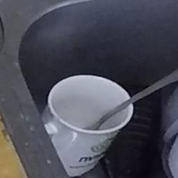
   Sphere 4 Finger
   Quadpod
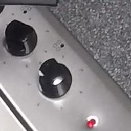
   Ring
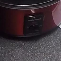
   Ventral
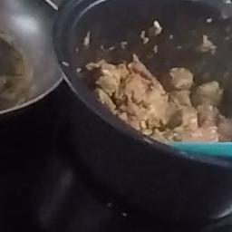
   Extension Type
   Small Diameter
   Prismatic 4 Finger

   Figure S14: Visualizations for Afforded Grasps. Top detections for selected hand grasp types on the validation split of EPIC-ROI dataset. We convert predicted grasp-specific heatmaps into detections (by finding scale-space blobs in the heatmaps) and visualize the top scoring detections across the validation dataset. Many of these detections are plausible, e.g. lid handles for power sphere, and sphere 4 finger grasps; bottle caps and stove knobs for quadpod grasp.

3. In Figure S15, we show the top detections for each of the 7 grasps made by ACP on the validation set of GAO benchmark. The images are colored green if the corresponding grasp is applicable to the highlighted object or else colored in red. We observe that for many hand-grasp types, the top scoring objects actually afford the corresponding hand-grasp type.

   

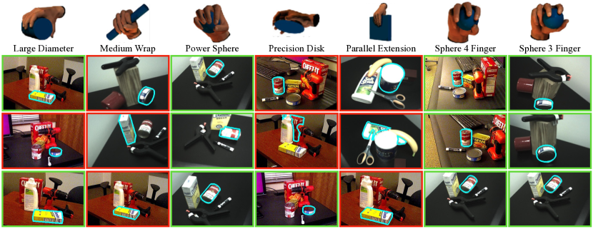
   Figure S15: Visualizations of predictions for GAO task on YCB-Affordance dataset. Here we show the top predictions (object-wise) made by ACP for the 7 grasps contained in the validation set. For each of the 7 grasps, we visualize the grasp (reproduced from [15]) in the top row, and show the top three predictions (after removing images that were very similar). We highlight the object for which the prediction is being made for (in cyan). We color the image frame to indicate correctness of prediction based on ground truth from Corona et al. [9] (green indicates correct, red indicates incorrect).

References

- [1] Andrea Bandini and José Zariffa. Analysis of the hands in egocentric vision: A survey. IEEE Transactions on Pattern Analysis and Machine Intelligence (TPAMI), 2020.
- [2] Samarth Brahmbhatt, Cusuh Ham, Charles C Kemp, and James Hays. Contactdb: Analyzing and predicting grasp contact via thermal imaging. In Proceedings of the IEEE Conference on Computer Vision and Pattern Recognition (CVPR), pages 8709–8719, 2019.
- [3] Minjie Cai, Kris M Kitani, and Yoichi Sato. Understanding hand-object manipulation with grasp types and object attributes. In Robotics: Science and Systems (RSS), volume 3. Ann Arbor, Michigan;, 2016.
- [4] Zhe Cao, Ilija Radosavovic, Angjoo Kanazawa, and Jitendra Malik. Reconstructing hand-object interactions in the wild. In Proceedings of the IEEE International Conference on Computer Vision (ICCV), 2021.
- [5] Mathilde Caron, Ishan Misra, Julien Mairal, Priya Goyal, Piotr Bojanowski, and Armand Joulin. Unsupervised learning of visual features by contrasting cluster assignments. In Advances in Neural Information Processing Systems (NeurIPS), 2020.
- [6] Ting Chen, Simon Kornblith, Mohammad Norouzi, and Geoffrey Hinton. A simple framework for contrastive learning of visual representations. In Proceedings of the International Conference on Machine Learning (ICML), pages 1597–1607. PMLR, 2020.
- [7] Xinlei Chen, Haoqi Fan, Ross Girshick, and Kaiming He. Improved baselines with momentum contrastive learning. arXiv preprint arXiv:2003.04297, 2020.
- [8] Xinlei Chen and Kaiming He. Exploring simple siamese representation learning. In Proceedings of the IEEE Conference on Computer Vision and Pattern Recognition (CVPR), 2021.
- [9] Enric Corona, Albert Pumarola, Guillem Alenya, Francesc Moreno-Noguer, and Gregory Rogez. Ganhand: Predicting human grasp affordances in multi-object scenes. In Proceedings of the IEEE Conference on Computer Vision and Pattern Recognition (CVPR), June 2020.
- [10] Dima Damen, Hazel Doughty, Giovanni Maria Farinella, Sanja Fidler, Antonino Furnari, Evangelos Kazakos, Davide Moltisanti, Jonathan Munro, Toby Perrett, Will Price, and Michael Wray. The epic-kitchens dataset: Collection, challenges and baselines. IEEE Transactions on Pattern Analysis and Machine Intelligence (TPAMI), 2020.
- [11] Dima Damen, Teesid Leelasawassuk, and Walterio Mayol-Cuevas. You-Do, I-Learn: Egocentric unsupervised discovery of objects and their modes of interaction towards video-based guidance. Computer Vision and Image Understanding, 149:98–112, 2016.
- [12] Carl Doersch, Abhinav Gupta, and Alexei A Efros. Unsupervised visual representation learning by context prediction. In Proceedings of the IEEE International Conference on Computer Vision (ICCV), pages 1422–1430, 2015.
- [13] Kiana Ehsani, Shubham Tulsiani, Saurabh Gupta, Ali Farhadi, and Abhinav Gupta. Use the force, luke! learning to predict physical forces by simulating effects. In Proceedings of the IEEE Conference on Computer Vision and Pattern Recognition (CVPR), pages 224–233, 2020.
- [14] Kuan Fang, Te-Lin Wu, Daniel Yang, Silvio Savarese, and Joseph J. Lim. Demo2vec: Reasoning object affordances from online videos. In Proceedings of the IEEE Conference on Computer Vision and Pattern Recognition (CVPR), June 2018.
- [15] Thomas Feix, Javier Romero, Heinz-Bodo Schmiedmayer, Aaron M Dollar, and Danica Kragic. The grasp taxonomy of human grasp types. IEEE Transactions on human-machine systems, 46(1):66–77, 2015.
- [16] David F Fouhey, Vincent Delaitre, Abhinav Gupta, Alexei A Efros, Ivan Laptev, and Josef Sivic. People watching: Human actions as a cue for single view geometry. In Proceedings of the European Conference on Computer Vision (ECCV), pages 732–745. Springer, 2012.
- [17] Guillermo Garcia-Hernando, Shanxin Yuan, Seungryul Baek, and Tae-Kyun Kim. First-person hand action benchmark with rgb-d videos and 3d hand pose annotations. In Proceedings of the IEEE Conference on Computer Vision and Pattern Recognition (CVPR), pages 409–419, 2018.
- [18] Shiry Ginosar, Amir Bar, Gefen Kohavi, Caroline Chan, Andrew Owens, and Jitendra Malik. Learning individual styles of conversational gesture. In Proceedings of the IEEE Conference on Computer Vision and Pattern Recognition (CVPR), pages 3497–3506, 2019.
- [19] Jean-Bastien Grill, Florian Strub, Florent Altché, Corentin Tallec, Pierre Richemond, Elena Buchatskaya, Carl Doersch, Bernardo Avila Pires, Zhaohan Guo, Mohammad Gheshlaghi Azar, Bilal Piot, koray kavukcuoglu, Remi Munos, and Michal Valko. Bootstrap your own latent - a new approach to self-supervised learning. In Advances in Neural Information Processing Systems (NeurIPS), 2020.
- [20] Henning Hamer, Juergen Gall, Thibaut Weise, and Luc Van Gool. An object-dependent hand pose prior from sparse training data. In Proceedings of the IEEE Conference on Computer Vision and Pattern Recognition (CVPR), pages 671–678, 2010.
- [21] Yana Hasson, Gul Varol, Dimitrios Tzionas, Igor Kalevatykh, Michael J Black, Ivan Laptev, and Cordelia Schmid. Learning joint reconstruction of hands and manipulated objects. In Proceedings of the IEEE Conference on Computer Vision and Pattern Recognition (CVPR), pages 11807–11816, 2019.
- [22] Kaiming He, Georgia Gkioxari, Piotr Dollár, and Ross Girshick. Mask R-CNN. In Proceedings of the IEEE Conference on Computer Vision and Pattern Recognition (CVPR), pages 2961–2969, 2017.
- [23] Kaiming He, Xiangyu Zhang, Shaoqing Ren, and Jian Sun. Deep residual learning for image recognition. In Proceedings of the IEEE Conference on Computer Vision and Pattern Recognition (CVPR), pages 770–778, 2016.
- [24] Phillip Isola, Joseph J Lim, and Edward H Adelson. Discovering states and transformations in image collections. In Proceedings of the IEEE Conference on Computer Vision and Pattern Recognition (CVPR), pages 1383–1391, 2015.
- [25] Hanwen Jiang, Shaowei Liu, Jiashun Wang, and Xiaolong Wang. Hand-object contact consistency reasoning for human grasps generation. In Proceedings of the IEEE International Conference on Computer Vision (ICCV), 2021.
- [26] Korrawe Karunratanakul, Jinlong Yang, Yan Zhang, Michael J. Black, Krikamol Muandet, and Siyu Tang. Grasping field: Learning implicit representations for human grasps. International Conference on 3D Vision (3DV), pages 333–344, 2020.
- [27] Kris M Kitani, Brian D Ziebart, James Andrew Bagnell, and Martial Hebert. Activity forecasting. In Proceedings of the European Conference on Computer Vision (ECCV), pages 201–214. Springer, 2012.
- [28] Mia Kokic, Danica Kragic, and Jeannette Bohg. Learning task-oriented grasping from human activity datasets. IEEE Robotics and Automation Letters, 5:3352–3359, 2020.
- [29] Hema S Koppula and Ashutosh Saxena. Physically grounded spatio-temporal object affordances. In Proceedings of the European Conference on Computer Vision (ECCV), pages 831–847. Springer, 2014.
- [30] Matthias Kummerer, Thomas S. A. Wallis, Leon A. Gatys, and Matthias Bethge. Understanding low- and high-level contributions to fixation prediction. In Proceedings of the IEEE International Conference on Computer Vision (ICCV), Oct 2017.
- [31] Taein Kwon, Bugra Tekin, Jan Stühmer, Federica Bogo, and Marc Pollefeys. H2o: Two hands manipulating objects for first person interaction recognition. In Proceedings of the IEEE/CVF International Conference on Computer Vision (ICCV), pages 10138–10148, October 2021.
- [32] Zihang Lai, Senthil Purushwalkam, and Abhinav Gupta. The functional correspondence problem. In Proceedings of the IEEE Conference on Computer Vision and Pattern Recognition (CVPR), pages 15772–15781, 2021.
- [33] Ian Lenz, Honglak Lee, and Ashutosh Saxena. Deep learning for detecting robotic grasps. The International Journal of Robotics Research, 34(4-5):705–724, 2015.
- [34] Sergey Levine, Peter Pastor, Alex Krizhevsky, Julian Ibarz, and Deirdre Quillen. Learning hand-eye coordination for robotic grasping with deep learning and large-scale data collection. The International Journal of Robotics Research, 37(4-5):421–436, 2018.
- [35] Bo Li, Wei Wu, Qiang Wang, Fangyi Zhang, Junliang Xing, and Junjie Yan. Siamrpn++: Evolution of siamese visual tracking with very deep networks. In Proceedings of the IEEE Conference on Computer Vision and Pattern Recognition (CVPR), 2019.
- [36] Xiaolong Li, He Wang, Li Yi, Leonidas J Guibas, A Lynn Abbott, and Shuran Song. Category-level articulated object pose estimation. In Proceedings of the IEEE Conference on Computer Vision and Pattern Recognition (CVPR), pages 3706–3715, 2020.
- [37] Jeffrey Mahler, Jacky Liang, Sherdil Niyaz, Michael Laskey, Richard Doan, Xinyu Liu, Juan Aparicio Ojea, and Ken Goldberg. Dex-net 2.0: Deep learning to plan robust grasps with synthetic point clouds and analytic grasp metrics. In Robotics: Science and Systems (RSS), 2017.
- [38] Priyanka Mandikal and Kristen Grauman. Dexterous robotic grasping with object-centric visual affordances. In Proceedings of the IEEE International Conference on Robotics and Automation (ICRA), 2021.
- [39] Priyanka Mandikal and Kristen Grauman. Dexvip: Learning dexterous grasping with human hand pose priors from video. In Proceedings of the Conference on Robot Learning (CoRL), 2021.
- [40] Kaichun Mo, Leonidas Guibas, Mustafa Mukadam, Abhinav Gupta, and Shubham Tulsiani. Where2act: From pixels to actions for articulated 3d objects. Proceedings of the IEEE International Conference on Computer Vision (ICCV), 2021.
- [41] Arsalan Mousavian, Clemens Eppner, and Dieter Fox. 6-dof graspnet: Variational grasp generation for object manipulation. In Proceedings of the IEEE International Conference on Computer Vision (ICCV), 2019.
- [42] Tushar Nagarajan, Christoph Feichtenhofer, and Kristen Grauman. Grounded human-object interaction hotspots from video. In Proceedings of the IEEE Conference on Computer Vision and Pattern Recognition (CVPR), pages 8688–8697, 2019.
- [43] Tushar Nagarajan and Kristen Grauman. Shaping embodied agent behavior with activity-context priors from egocentric video. In Advances in Neural Information Processing Systems (NeurIPS), 2021.
- [44] Tushar Nagarajan, Yanghao Li, Christoph Feichtenhofer, and Kristen Grauman. EGO-TOPO: Environment affordances from egocentric video. In Proceedings of the IEEE Conference on Computer Vision and Pattern Recognition (CVPR), pages 163–172, 2020.
- [45] Evonne Ng, Donglai Xiang, Hanbyul Joo, and Kristen Grauman. You2me: Inferring body pose in egocentric video via first and second person interactions. In Proceedings of the IEEE Conference on Computer Vision and Pattern Recognition (CVPR), pages 9890–9900, 2020.
- [46] Junting Pan, Cristian Canton-Ferrer, Kevin McGuinness, Noel E. O’Connor, Jordi Torres, Elisa Sayrol, and Xavier Giró-i-Nieto. Salgan: Visual saliency prediction with generative adversarial networks. CoRR, abs/1701.01081, 2017.
- [47] Deepak Pathak, Philipp Krähenbühl, Jeff Donahue, Trevor Darrell, and Alexei Efros. Context encoders: Feature learning by inpainting. In Proceedings of the IEEE Conference on Computer Vision and Pattern Recognition (CVPR), 2016.
- [48] Vladimír Petrík, Makarand Tapaswi, Ivan Laptev, and Josef Sivic. Learning object manipulation skills via approximate state estimation from real videos. Proceedings of the Conference on Robot Learning (CoRL), 2020.
- [49] Lerrel Pinto and Abhinav Gupta. Supersizing self-supervision: Learning to grasp from 50k tries and 700 robot hours. Proceedings of the IEEE International Conference on Robotics and Automation (ICRA), pages 3406–3413, 2016.
- [50] Nicholas Rhinehart and Kris M Kitani. First-person activity forecasting with online inverse reinforcement learning. In Proceedings of the IEEE International Conference on Computer Vision (ICCV), pages 3696–3705, 2017.
- [51] Grégory Rogez, James S Supancic, and Deva Ramanan. Understanding everyday hands in action from RGB-D images. In Proceedings of the IEEE Conference on Computer Vision and Pattern Recognition (CVPR), pages 3889–3897, 2015.
- [52] Karl Schmeckpeper, Oleh Rybkin, Kostas Daniilidis, Sergey Levine, and Chelsea Finn. Reinforcement learning with videos: Combining offline observations with interaction. In Proceedings of the Conference on Robot Learning (CoRL), 2020.
- [53] Pierre Sermanet, Corey Lynch, Yevgen Chebotar, Jasmine Hsu, Eric Jang, Stefan Schaal, Sergey Levine, and Google Brain. Time-contrastive networks: Self-supervised learning from video. In Proceedings of the IEEE International Conference on Robotics and Automation (ICRA), pages 1134–1141, 2018.
- [54] Pierre Sermanet, Kelvin Xu, and Sergey Levine. Unsupervised perceptual rewards for imitation learning. In Robotics: Science and Systems (RSS), 2017.
- [55] Dandan Shan, Jiaqi Geng, Michelle Shu, and David Fouhey. Understanding human hands in contact at internet scale. In Proceedings of the IEEE Conference on Computer Vision and Pattern Recognition (CVPR), 2020.
- [56] Dandan Shan, Richard E.L. Higgins, and David F. Fouhey. COHESIV: Contrastive object and hand embedding segmentation in video. In Advances in Neural Information Processing Systems (NeurIPS), 2021.
- [57] Jin Sun, Hadar Averbuch-Elor, Qianqian Wang, and Noah Snavely. Hidden footprints: Learning contextual walkability from 3d human trails. In Proceedings of the European Conference on Computer Vision (ECCV), pages 192–207. Springer, 2020.
- [58] Bugra Tekin, Federica Bogo, and Marc Pollefeys. H+ o: Unified egocentric recognition of 3d hand-object poses and interactions. In Proceedings of the IEEE Conference on Computer Vision and Pattern Recognition (CVPR), pages 4511–4520, 2019.
- [59] Spyridon Thermos, Gerasimos Potamianos, and Petros Daras. Joint object affordance reasoning and segmentation in rgb-d videos. IEEE Access, 9:89699–89713, 2021.
- [60] Suchen Wang, Kim-Hui Yap, Junsong Yuan, and Yap-Peng Tan. Discovering human interactions with novel objects via zero-shot learning. In Proceedings of the IEEE Conference on Computer Vision and Pattern Recognition (CVPR), 2020.
- [61] Xiaolong Wang, Rohit Girdhar, and Abhinav Gupta. Binge watching: Scaling affordance learning from sitcoms. In Proceedings of the IEEE Conference on Computer Vision and Pattern Recognition (CVPR), pages 2596–2605, 2017.
- [62] Yu Xiang, Tanner Schmidt, Venkatraman Narayanan, and Dieter Fox. PoseCNN: A convolutional neural network for 6d object pose estimation in cluttered scenes. In Robotics: Science and Systems (RSS), 2018.
- [63] Yezhou Yang, Cornelia Fermuller, Yi Li, and Yiannis Aloimonos. Grasp type revisited: A modern perspective on a classical feature for vision. In Proceedings of the IEEE Conference on Computer Vision and Pattern Recognition (CVPR), pages 400–408, 2015.
- [64] Kevin Zakka, Andy Zeng, Pete Florence, Jonathan Tompson, Jeannette Bohg, and Debidatta Dwibedi. Xirl: Cross-embodiment inverse reinforcement learning. In Proceedings of the Conference on Robot Learning (CoRL), 2021.
- [65] Richard Zhang, Phillip Isola, and Alexei A Efros. Split-brain autoencoders: Unsupervised learning by cross-channel prediction. In Proceedings of the IEEE Conference on Computer Vision and Pattern Recognition (CVPR), pages 1058–1067, 2017.
parttoc \mtcsettitleparttocHuman Hands as Probes for Interactive Object Understanding – Supplementary Material