Comment on the literature definition(s) of “dynamical phase transition”

Introduction. Dynamical phase transitions are often associated with a singular response of the dynamical large-deviation functions of a model, particularly a kink of the scaled cumulant-generating function (SCGF) Garrahan et al. (2009); Vaikuntanathan et al. (2014); Nemoto et al. (2017); Nyawo and Touchette (2017); Horowitz and Kulkarni (2017); Nyawo and Touchette (2018); Nemoto et al. (2019); Jack (2020). Such kinks are usually said to indicate the existence of a first-order dynamical phase transition and accompanying dynamical phase coexistence Garrahan et al. (2009); Jack (2020), by analogy with equillibrium systems Touchette (2009); Binney et al. (1992). Kinks can emerge in various settings, including the small-rate (reducible) limits of microscopic models Dinwoodie and Zabell (1992); Dinwoodie (1993); Coghi et al. (2019); Garrahan and Lesanovsky (2014); Whitelam (2018), and the large-size limit of lattice- or off-lattice models Garrahan et al. (2009); Nemoto et al. (2019); Buča et al. (2019).

There is not universal agreement about when the label “dynamical phase transition” applies: some authors consider to the term to be appropriate only in the large-size limit of a many-body system Buča et al. (2019); some consider that it also applies in the large-size limit of a one-body system Vaikuntanathan et al. (2014); Nemoto et al. (2017); and some apply the term to systems of finite size Nyawo and Touchette (2017); Horowitz and Kulkarni (2017). My view is that the setting in which the singularity emerges is less important than the phenomenology of the underlying model, which in some cases resembles that of an equilibrium system with distinct phases and in some cases does not. In this note I want to make a technical point about how dynamical phase transitions are diagnosed, comment on existing classification schemes, and offer some suggestions for how to clarify the nature of systems that display these kinks.

The limiting procedure often used to identify dynamical phase transitions is problematic. Some authors advocate an approach to dynamical large deviations in which time $T$ is interpreted as if it were a spatial coordinate of a thermodynamic system Jack (2020). In this approach, SCGF kinks that arise in a joint limit, in which first $T$ and then system size $N$ are taken infinite, are taken as evidence of a first-order dynamical or “space-time” phase transition, accompanied by dynamical phase coexistence. I have argued previously that large-deviation singularities are not necessarily accompanied by phase-transition-like behavior: singularities can occur if a system is simply slow, whether or not it supports multiple phases Whitelam (2018); Whitelam and Jacobson (2021). Here I revisit this point in the context of the many-body system of Ref. Buča et al. (2019), which in the double limit displays a singularity that the authors argue indicates a phase transition. I argue instead that that the double-limit procedure produces a breakdown of the large-deviation principle (LDP), from which little can be determined. However, it is possible to take the large-size limit of the model in a way that restores the LDP, and this picture, combined with numerical simulations of the model presented in the paper, does not provide strong evidence for coexisting phases.

The authors of Ref. Buča et al. (2019) take the long-time limit in order to obtain the SCGF, $\theta_{N}(s)$, of a particular time-integrated observable ($s$ is the Legendre-transform parameter), and then take the large-$N$ limit. The result is a kinked $\theta_{N}(s)$ and a set of large-deviation functions reminiscent of those of the Ising model below its critical temperature, which does display phase coexistence Binney et al. (1992); Touchette (2009). However, several aspects of these functions are inconsistent with known features of the model.

Principally, the model has a well-defined mean or typical value of the chosen observable, Eq. (8) of the paper, even in the limit $N\to\infty$. However, the function $\lim_{N\to\infty}N^{-1}\theta_{N}(s)$, Eq. (10) of the paper, does not know this: it is not differentiable at the origin, and contains none of the model parameters $\alpha$ to $\delta$ that appear in Eq. (8). The function $\lim_{N\to\infty}N^{-1}\theta_{N}(s)$ cannot generate the first cumulant, and so therefore cannot be the cumulant-generating function. Equivalently, the rate function associated with Eq. (10) possesses a line of zeros. If a large deviation principle applies, we would expect a rate function with a unique zero that corresponds to the model’s typical behavior Den Hollander (2008); Touchette (2009).

I argue that this model is described by a large-deviation principle, even in the limit $N\to\infty$, but on a different scale to the one examined in the paper. We can look for a large-deviation principle with large parameter (or speed) $\tilde{T}\equiv T/\tau(N)$, where $\tau(N)$ is the dominant model timescale, by writing $P_{T}\sim\exp(-T\varphi_{N}(x))\equiv\exp(-\tilde{T}\tilde{\varphi}_{N}(x))$, where $P_{T}$ is the probability of observing a particular value $x$ of te observable. The rate function on speed $\tilde{T}$ is $\tilde{\varphi}_{N}=\tau(N)\varphi_{N}$. The corresponding SCGF is obtained by sending $s\to s/\tau(N)$, giving the function $\theta_{N}(s/\tau(N))$.

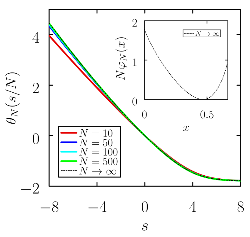
Figure 1: Large-deviation functions of the boundary-driven cellular automaton of Ref. Buča et al. (2019) on speed $T/N$. The data collapse in the large-$N$ limit indicates the existence of a well-defined large-deviation principle. Inset: limiting form of the corresponding rate function, which quantifies the logarithmic probability of observing a value $x$ of the dynamical observable studied in that paper. The unique zero corresponds to the model’s typical behavior.

Given that the model’s dynamics is ballistic, I assume $\tau(N)=N$, and plot in Fig. 1 the large-deviation functions on speed $\tilde{T}=T/N$. As $N$ becomes large, these functions tend to a limiting, non-singular form. The colored lines were produced by numerically evaluating Eq. (4) of Ref. Buča et al. (2019). The black dashed line was produced by taking the limit $N\to\infty$ analytically (having first sent $s\to s/N$) and then evaluating the resulting equation numerically. The resulting function is the limiting form to which the SCGF tends. The inset of Fig. 1 shows the corresponding limiting rate function, $\lim_{N\to\infty}\tilde{\varphi}_{N}(x)$, which quantifies the logarithmic probability of observing certain values $x$ of the time-integrated observable. As expected from a well-defined large-deviation principle, this has a unique zero corresponding to the typical value of the observable, Eq. (8) of the paper. That is, the limiting analytic procedure consistent with a well-defined large-deviation principle is to take $T\to\infty$, then rescale the Legendre-transform parameter $s$ by the system’s dominant timescale, and then take $N\to\infty$. Similar considerations apply to a random-walk model in the large-size limit Whitelam and Jacobson (2021), and to finite-size models in the small-rate limit Whitelam (2018).

Does this model exhibit phase coexistence? One way a system could be said to exhibit coexisting dynamical phases is if the probability of observing trajectories of distinct values of a time-integrated observable are equal and special in some way (see e.g. the right-hand panel of Fig. 6 of Ref. Whitelam and Jacobson (2021)). The limiting functions displayed in Ref. Buča et al. (2019) suggest that dynamical trajectories corresponding to large or small values of the chosen observable become increasingly prominent or important as the system is made larger, at least by analogy with the Ising model. My reservation with this analogy is that it is based principally on the fact that the LDP breaks down for both models, rather than an assessment of the physics of each. We know from elementary considerations that the Ising model below its critical temperature has two typical behaviors, which can be identified on the scale $\sqrt{N}$ (in 2D) Binney et al. (1992); Touchette (2009), while the dynamical model has one, which can be identified on the scale $T/\tau(N)$. The logarithmic probability of observing trajectories with values $x$ of the observable is $T/\tau(N)$ multiplied by the function shown in the inset of Fig. 1, which resembles that of a Poisson-like process with a large timescale, and does not support the idea of coexisting values of $x$.

Another way a system could be said to exhibit coexistence is if the trajectories that realize particular values of the time-integrated observable are intermittent, interconverting between different values of the instantaneous quantity that comprises the time-integrated observable (see e.g. the middle panel of Fig. 6 of Ref. Whitelam and Jacobson (2021)). Whether or not this is the case cannot be deduced directly from the rate function , and must be assessed by direct calculation of those trajectories. The authors of Ref. Buča et al. (2019) rule out this scenario in the text, and show in Fig. 3 some rare trajectories of the model; these are not intermittent.

To summarize, kinked large-deviation functions that emerge in the double-limit procedure of Ref. Jack (2020) are not necessarily diagnostic of phase coexistence, and are caused for the model of Ref. Buča et al. (2019) by a breakdown of the large-deviation principle. The idea of phase coexistence in this model is not supported by the large-deviation functions that result from a limiting procedure modified to restore the LDP, or by the nature of the rare dynamical trajectories calculated in Ref. Buča et al. (2019). I would argue that the evidence points toward this model having dynamics that slows with increasing system size, not cooperative behavior reminiscent of a phase transition.

Existing classification schemes tend to focus on how the singularity emerges, rather than the underlying model phenomenology. Fig. 2 shows some examples of systems described in the literature as having dynamical phase transitions. It is incomplete (e.g. some systems show singularities away from any limit Nyawo and Touchette (2017)), but captures some of the more common types of behavior. Although each system is described as a phase transition by the authors who study it, because of the presence of a large-deviation singularity, there is not consensus among this group as to whether application of the label should depend upon the limit in which the singularity arises. The label is more likely to be applied to systems as we move downwards on Fig. 2, because equilibrium phase transitions occur in the large-system-size limit of many-body systems.

Aside from issues of consistency, one problem with classification-by-singularity is that it is insensitive to phenomenology: the label “phase transition” can then be applied to models that are simply slow, and display no features that could be said to resemble distinct phases. The label can also be applied to systems with intermittent conditioned trajectories, which are more phase-transition-like, their behavior in the long-time limit resembling the static behavior of the 1D Ising model at nonzero temperature (which, however, does not exhibit true phase coexistence in equilibrium terms). There also exist models with cooperative dynamics, much as the Ising model has cooperative interactions. These models display large-deviation singularities and phase-transition-like phenomenology that includes a change of typical behavior with a change of model parameters, and a breaking of ergodicity accompanied by the emergence of multiple dynamical phases Klymko et al. (2017); Whitelam and Jacobson (2021). However, some authors argue that such behavior should not be called a phase transition Jack (2019), and so it is possible to find literature definitions of “dynamical phase transition” that are essentially anticorrelated with the existence of phase-transition-like phenomenology.

My view is that a more physically meaningful way to classify systems that display large-deviation singularities is by phenomenology. All are different to equilibrium systems in some respects, but we can compare the ways in which their dynamics is similar to the cooperative behavior of an equilibrium system that displays a phase transition. By this measure the degree to which models exhibit phase-transition-like behavior increases from left to right in Fig. 2 (excepting the first column, which indicates systems yet to be classified). The precise dividing line between what we call a dynamical phase transition and what we do not is a matter of interpretation, but in my view should be based on the physics of the model under study.

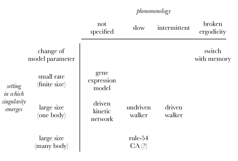
Figure 2: Examples of models that exhibit large-deviation singularities: a model of gene expression Horowitz and Kulkarni (2017), a driven kinetic network Vaikuntanathan et al. (2014), undriven Whitelam and Jacobson (2021)- and driven Nemoto et al. (2017); Whitelam and Jacobson (2021) random walkers, a cellular automaton Buča et al. (2019), and a switch with memory (or growth model) Klymko et al. (2017); Whitelam and Jacobson (2021). All are described in the papers indicated as displaying phase transitions, but consensus between these groups of authors does not exist.

Absent a consistent classification scheme, one point that could be better clarified in the literature is the meaning of a kinked large-deviation function. If singular behavior is diagnosed in some limit, is this limit consistent with known features of the model, such as its typical behavior? Does the LDP break down entirely, or is there a well-defined LDP on some speed or speeds? Does the kink signal the emergence of distinct trajectory types whose probabilities are equal, or intermittency within a trajectory, or slow dynamics, or some other type of behavior? If the conditioned dynamics of the model is intermittent, what are the dynamical “phases” that contribute to the intermittency? Why on physical grounds does the system adopt this behavior in order to achieve, in the least unlikely way, a particular value of a time-integrated observable (see the discussion of Sec. IV of Ref. Whitelam and Jacobson (2021))?

Acknowledgment. This work was performed at the Molecular Foundry, Lawrence Berkeley National Laboratory, supported by the Office of Science, Office of Basic Energy Sciences, of the U.S. Department of Energy under Contract No. DE-AC02–05CH11231.

References

- Garrahan et al. (2009) Juan P Garrahan, Robert L Jack, Vivien Lecomte, Estelle Pitard, Kristina van Duijvendijk, and Frédéric van Wijland, “First-order dynamical phase transition in models of glasses: an approach based on ensembles of histories,” Journal of Physics A: Mathematical and Theoretical 42, 075007 (2009).
- Vaikuntanathan et al. (2014) Suriyanarayanan Vaikuntanathan, Todd R Gingrich, and Phillip L Geissler, “Dynamic phase transitions in simple driven kinetic networks,” Physical Review E 89, 062108 (2014).
- Nemoto et al. (2017) Takahiro Nemoto, Robert L Jack, and Vivien Lecomte, “Finite-size scaling of a first-order dynamical phase transition: Adaptive population dynamics and an effective model,” Physical Review Letters 118, 115702 (2017).
- Nyawo and Touchette (2017) Pelerine Tsobgni Nyawo and Hugo Touchette, “A minimal model of dynamical phase transition,” EPL (EuroPhysics Letters) 116, 50009 (2017).
- Horowitz and Kulkarni (2017) Jordan M Horowitz and Rahul V Kulkarni, “Stochastic gene expression conditioned on large deviations,” Physical biology 14, 03LT01 (2017).
- Nyawo and Touchette (2018) Pelerine Tsobgni Nyawo and Hugo Touchette, “Dynamical phase transition in drifted brownian motion,” Physical Review E 98, 052103 (2018).
- Nemoto et al. (2019) Takahiro Nemoto, Étienne Fodor, Michael E Cates, Robert L Jack, and Julien Tailleur, “Optimizing active work: Dynamical phase transitions, collective motion, and jamming,” Physical Review E 99, 022605 (2019).
- Jack (2020) Robert L Jack, “Ergodicity and large deviations in physical systems with stochastic dynamics,” The European Physical Journal B 93, 1–22 (2020).
- Touchette (2009) Hugo Touchette, “The large deviation approach to statistical mechanics,” Physics Reports 478, 1–69 (2009).
- Binney et al. (1992) James J Binney, NJ Dowrick, AJ Fisher, and M Newman, The theory of critical phenomena: an introduction to the renormalization group (Oxford University Press, Inc., 1992).
- Dinwoodie and Zabell (1992) I. H. Dinwoodie and S. L. Zabell, “Large deviations for exchangeable random vectors,” The Annals of Probability 20, 1147–1166 (1992).
- Dinwoodie (1993) I. H. Dinwoodie, “Identifying a large deviation rate function,” Annals of probability 21, 216–231 (1993).
- Coghi et al. (2019) Francesco Coghi, Jules Morand, and Hugo Touchette, “Large deviations of random walks on random graphs,” Physical Review E 99, 022137 (2019).
- Garrahan and Lesanovsky (2014) Juan P Garrahan and Igor Lesanovsky, “Comment on “abrupt transition in the structural formation of interconnected network”, Nat. Phys. 9, 717 (2013),” arXiv preprint arXiv:1406.4706 (2014).
- Whitelam (2018) Stephen Whitelam, “Large deviations in the presence of cooperativity and slow dynamics,” Physical Review E 97, 062109 (2018).
- Buča et al. (2019) Berislav Buča, Juan P Garrahan, Tomaž Prosen, and Matthieu Vanicat, “Exact large deviation statistics and trajectory phase transition of a deterministic boundary driven cellular automaton,” Physical Review E 100, 020103 (2019).
- Whitelam and Jacobson (2021) Stephen Whitelam and Daniel Jacobson, “Varied phenomenology of models displaying dynamical large-deviation singularities,” Physical Review E 103, 032152 (2021).
- Den Hollander (2008) Frank Den Hollander, Large Deviations, Vol. 14 (American Mathematical Soc., 2008).
- Note (1) A linear nonvanishing rate function is suggestive of intermittency, although linear rate functions can also arise in other contexts Touchette (2009).
- Klymko et al. (2017) Katherine Klymko, Juan P Garrahan, and Stephen Whitelam, “Similarity of ensembles of trajectories of reversible and irreversible growth processes,” Physical Review E 96, 042126 (2017).
- Jack (2019) Robert L Jack, “Large deviations in models of growing clusters with symmetry-breaking transitions,” Physical Review E 100, 012140 (2019).