Evaluating Lyman-$\alpha$ Constraints for General Dark-Matter Velocity Distributions:
Multiple Scales and Cautionary Tales

Abstract

One of the most important observational constraints on possible models of dark-matter physics exploits the Lyman-$\alpha$ absorption spectrum associated with photons traversing the intergalactic medium. Because this data allows us to probe the linear matter power spectrum with great accuracy down to relatively small distance scales, finding ways of accurately evaluating such Lyman-$\alpha$ constraints across large classes of candidate models of dark-matter physics is of paramount importance. While such Lyman-$\alpha$ constraints have been evaluated for dark-matter models that give rise to relatively simple dark-matter velocity distributions, more complex models — particularly those whose dark-matter velocity distributions stretch across multiple scales — have recently been receiving increasing attention. In this paper, we undertake a study of the Lyman-$\alpha$ constraints associated with general dark-matter velocity distributions. Although such Lyman-$\alpha$ constraints are difficult to evaluate in principle, in practice there currently exist two classes of methods in the literature through which such constraints can be recast into forms which are easier to evaluate and which therefore allow a more rapid determination of whether a given dark-matter model is ruled in or out. Accordingly, we utilize both of these recasts in order to determine the Lyman-$\alpha$ bounds on different classes of dark-matter velocity distributions. We also develop a general method by which the results of these different recasts can be compared. For relatively simple dark-matter velocity distributions, we demonstrate that these two classes of recasts tend to align and give similar results. However, we find that the situation is far more complex for distributions involving multiple velocity scales: while these two classes of recasts continue to yield similar results within certain regions of parameter space, they nevertheless yield dramatically different results within precisely those regions of parameter space which are likely to be phenomenologically relevant. This, then, serves as a cautionary tale regarding the use of such recasts for complex dark-matter velocity distributions.

I Introduction

On large scales, the $\Lambda$CDM cosmology — a cosmology which is built on a relatively simple set of assumptions and whose components include only ordinary (visible) matter, cold dark matter (CDM), and a cosmological constant $\Lambda$ — has provided a remarkably successful model of the universe [1]. However, on smaller scales corresponding to distances $\lesssim 1\,\text{Mpc}$, evidence of this success is not as solid, with inconsistencies between numerical simulations and observations [2, 3, 4, 5] appearing in several areas.

Several of these inconsistencies can potentially be addressed by positing that the dark matter is not strictly cold. Indeed, there exist a variety of mechanisms through which a population of dark-matter particles with a non-negligible primordial velocity distribution can be produced in the early universe. However, different mechanisms can give rise to different velocity distributions with dramatically different shapes.

In order to illustrate the range of possibilities, in Fig. 1 we provide two examples of possible dark-matter velocity distributions which arise in different dark-matter scenarios. The first of these distributions (dashed gray curve) arises from a warm dark matter (WDM) scenario wherein a dark-matter particle with a mass of $\mathcal{O}({\rm keV})$ is produced via thermal freeze-out while still relativistic. It is a simple, unimodal distribution which is sharply peaked around a particular velocity. The second distribution (solid blue curve), by contrast, arises within the context of a dark-matter model [6] in which the dark matter is produced as the end-product of a long sequence of possible decays that take place within a tower of heavier, unstable dark states. The non-trivial shape of the resulting dark-matter velocity distribution then reflects the contributions of many possible decay chains within such a scenario. Indeed, the resulting dark-matter velocity distribution can be highly complex and even multi-modal. We emphasize that both of the distributions shown in Fig. 1 have the same average velocity and would naïvely be characterized by the same free-streaming horizon $k_{\rm FSH}\approx 1.1\,h/\text{Mpc}$, where $h$ is the dimensionless Hubble constant. However, they also clearly differ significantly and indeed give rise to different predictions for small-scale structure — even for the same background cosmology.

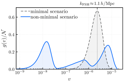
Figure 1: Examples of possible dark-matter velocity distributions $g(v)/\mathcal{N}$ which lead to departures from the small-scale structure predicted by CDM.  The dashed gray curve represents the distribution which arises from the thermal freeze-out of a dark-matter particle with a mass of $\mathcal{O}({\rm keV})$. By contrast, the solid blue curve represents a highly non-thermal velocity distribution generated by decay cascades within a non-minimal dark sector [6]. Both of the distributions shown have the same present-day average velocity and would naïvely be characterized by the same free-streaming horizon $k_{\rm FSH}\approx 1.1\,h/\text{Mpc}$.

One way in which the detailed structure of the primordial dark-matter velocity distribution leaves its imprint on small-scale structure is through free-streaming effects, which impact the shape of the linear matter power spectrum. Indeed, a great deal of information about the velocity distribution can be inferred from the shape of the matter power spectrum directly. That said, deriving rigorous constraints on the dark-matter velocity distribution in this way presents some challenges. One such challenge stems from the fact that the Lyman-$\alpha$ forest currently provides the most stringent constraints on the shape of the matter power spectrum across a broad range of comoving wavenumbers $k$. In order to translate these Lyman-$\alpha$ constraints into rigorous bounds on any particular dark-matter model, one would typically need to perform detailed numerical hydrodynamic simulations specifically tailored to that model and its characteristic dark-matter velocity distribution. Since simulations of this sort are computationally intensive, it is impractical to employ them when surveying broad classes of dark-matter models.

For this reason, methods for evaluating these constraints have been developed which effectively involve recasting the Lyman-$\alpha$ data onto a baseline WDM model for which these sorts of hydrodynamic simulations have already been carried out. Different methods exist in the literature for constructing such recasts, but these methods typically fall into two general classes. The first class comprises methods which are sensitive to the properties of the power spectrum only at relatively low values of $k$ [7, 8, 9, 10, 11, 12, 13, 14, 15, 16, 17, 18]. By contrast, the second class comprises methods which are sensitive to the properties of $T(k)$ over a broader range of $k$ [19, 20, 21, 22, 23, 24, 25, 26, 27, 28, 29]. We shall refer to recasts which fall into these two classes as “half-mode” and $\delta A$ recasts, respectively. The methods involved in formulating recasts within each class will be reviewed in Sect. II.

In this paper, we shall utilize these recasts in order to undertake a general study of Lyman-$\alpha$ constraints on dark-matter models which transcend the traditional CDM hypothesis. More specifically, we shall utilize these recasts in order to evaluate the Lyman-$\alpha$ constraints for a variety of dark-matter velocity distributions. Given that both half-mode and $\delta A$ recasts are constructed in reference to a baseline WDM velocity distribution, we shall find it useful to classify the different possible dark-matter velocity distributions that we shall examine in this paper into two overall categories:

• Class I: velocity distributions whose shapes are well approximated by the characteristic profile which arises in WDM scenarios. Such velocity distributions have a single peak, as exemplified by the unimodal distribution depicted in Fig. 1, and rise and fall smoothly from that peak on either side.

• Class II: more complicated velocity distributions whose shapes depart significantly from the WDM profile. Such distributions exhibit a variety of different internal features, and include multi-modal distributions of the sort illustrated in Fig. 1.

We shall begin our analysis by examining the Lyman-$\alpha$ constraints on dark-matter scenarios whose characteristic velocity distributions unambiguously fall within Class I. By definition, these include the baseline WDM scenario itself. We shall then systematically study departures from this baseline scenario and investigate how the Lyman-$\alpha$ constraints vary as the shape of the dark-matter velocity distribution is modified. Finally, fully breaking from Class I, we examine the constraints on dark-matter scenarios which give rise to multi-modal velocity distributions — distributions which decidedly fall within Class II.

Because we shall employ both the half-mode and $\delta A$ recasts in our analysis, the results of our paper will also enable us to compare these two classes of recasts. For Class-I velocity distributions, we find that these recasts tend to align and give similar results. However, we find that the situation is far more complex for Class II velocity distributions. While the two classes of recasts continue to yield similar results within certain regions of parameter space, they can nevertheless yield dramatically different results within precisely those regions of parameter space which are likely to be phenomenologically relevant. Indeed, these differences can be quite significant. Our results thus provide a cautionary tale regarding the use of such recasts when more general velocity distributions are considered.

This paper is organized as follows. In Sect. II, we begin by reviewing the calculations necessary in order to evaluate the Lyman-$\alpha$ constraints on dark-matter models. We also outline the two classes of recasts that we consider in this paper. In Sect. III, we then develop a general method through which these two recasts can be compared on an equal footing. In Sect. IV, we evaluate the Lyman-$\alpha$ constraints obtained from both of these recasts for a simple baseline dark-matter model as well as for certain extensions of this model. In Sect. V, we then turn our attention to non-minimal dark-matter scenarios in which the dark-matter velocity distribution is multi-modal and compare the results obtained from our two recasts within such scenarios. In Sect. VI, we apply a parametric function for multi-modal distributions. Finally, in Sect. VII, we discuss the potential implications of our results and identify areas meriting further exploration.

II Evaluating Lyman-$\alpha$ Constraints on Dark Matter

Given a proposed model of dark-matter physics and a given background cosmology, one can in principle calculate the spatial distribution of dark matter within and between galaxies. The spatial distribution of dark matter affects the spatial distribution of visible matter — including the frequency and density of clouds of neutral hydrogen — which can be probed by astronomical observations. In particular, as light emanating from distant quasars and other bright objects passes through the intergalactic medium, it interacts with the neutral hydrogen and can be observed today. By analyzing the Lyman-$\alpha$ absorption spectrum of this radiation, one can infer properties of the hydrogen distribution. In this way, measurements of the observed Lyman-$\alpha$  absorption spectrum within such light can indirectly be used to constrain models of dark-matter physics.

As we shall see, the central object in evaluating such Lyman-$\alpha$ constraints is the so-called “transfer function” $T(k)$. For any model of dark-matter physics with a predicted linear matter power spectrum $P(k)$, or for any set of cosmological observations that yield an observed linear matter power spectrum $P(k)$, the corresponding transfer function $T(k)$ is defined as

$$T^{2}(k)~{}\equiv~{}\frac{P(k)}{P_{\rm CDM}(k)}~{}$$ (1)

where $P_{\rm CDM}(k)$ is the matter power spectrum that would have arisen in a model consisting of purely cold dark matter and where $k$ once again denotes a comoving wavenumber. The transfer function thus tracks how cosmological structure, either in theoretical predictions or in data gathered from observations, deviates from that of CDM.

In general, in order to evaluate Lyman-$\alpha$ constraints on a given dark-matter model, one is faced with two tasks. The first is to determine the transfer function $T(k)$ predicted by the theoretical dark-matter model; the second is to translate observational data in such a way that it may be compared directly to these predictions. We shall now provide a brief outline of how these tasks are typically performed.

II.1 Determining Theoretical Predictions for $T(k)$

In general, the form of $T(k)$ which arises from any particle-physics model of dark matter depends on a variety of factors. One of the most important is the dark-matter phase-space distribution $g(p,t)$, which in an approximately homogeneous and isotropic universe can be expressed in terms of the three-momentum magnitude $p\equiv\left|\vec{p}\hskip 0.56905pt\right|$ and the time $t$ alone. We shall find it convenient to define $g(p,t)$ as a distribution in $(\log p)$-space according to the relation

$$N(t)~{}=~{}{g_{\rm int}\over 2\pi^{2}}\int_{-\infty}^{\infty}\!\!d\log p~{}g(p,t)\ ,$$ (2)

where $N(t)$ is the comoving number density of the particle species which constitutes the dark matter and where $g_{\rm int}$ is the number of internal degrees of freedom for that species. With this definition for $g(p,t)$, cosmological redshifting does not alter the shape of $g(p,t)$, but instead merely shifts the entire distribution uniformly to lower values of $\log p$.

For many dark-matter models, $g(p,t)$ effectively ceases evolving — except in the trivial way discussed above, as a consequence of cosmological redshifting — well before the time ${t_{\rm MRE}}$ of matter-radiation equality. For such models, one may unambiguously characterize the primordial dark-matter velocity distribution in terms of the distribution $g(p)\equiv g(p,t_{\mathrm{now}})$, where the extrapolation of $g(p,t)$ to the present time $t_{\mathrm{now}}$ is performed accounting for cosmological redshifting alone. Indeed, this $g(p)$ distribution tells us whether the dark matter is cold or hot, thermal or non-thermal, and so forth. Moreover, the functional form for $g(p)$ contains all of the information we require in order to calculate the corresponding transfer function directly by evolving the spectrum of primordial cosmological perturbations forward in time. In this paper, we shall carry out calculations of this sort using the CLASS software package [30, 31, 32, 33].

Since $g(p)$ contains all of the information necessary to produce predictions for $T(k)$, we can survey large classes of dark-matter models simply by examining different possible profiles for $g(p)$ without worrying about the underlying physics from which these distributions might ultimately have been produced. Indeed, while many details of the underlying physics leave unique imprints on the $g(p)$ distributions, many features do not. This issue is studied in some detail in Ref. [6].

Our primary interest in this paper is to investigate how dark-matter models with different $g(p)$ distributions are constrained by Lyman-$\alpha$ data. As such, we are primarily interested in $g(p)$ distributions for which free-streaming effects have an impact on structure on scales that can be meaningfully probed using such data. For a Class-I distribution, the effect of free-streaming on $P(k)$ is comparatively straightforward to assess. The primary figure of merit in this regard is the present-day value $\left\langle v\right\rangle=\left\langle v(t_{\mathrm{now}})\right\rangle$ of the time-dependent average velocity

$$\left\langle v(t)\right\rangle\!~{}=~{}\frac{2\pi^{2}}{g_{\rm int}}\int_{-\infty}^{\infty}d\log p\,\frac{p}{\sqrt{p^{2}+m^{2}a^{2}(t)}}\,g(p)~{},~{}$$ (3)

where $a(t)$ is the scale factor, defined such that $a(t_{\mathrm{now}})=1$. In particular, for such distributions, one may sensibly define the free-streaming horizon

$$d_{\rm FSH}~{} \equiv~{}\int\frac{dt}{a(t)}\left\langle v(t)\right\rangle$$

$$\approx~{}\frac{\left\langle v\right\rangle}{(a^{2}H)_{\rm MRE}}\left[2+\log\left(\!\frac{2a_{\rm MRE}}{\left\langle v\right\rangle}\!\right)\right]\ ,$$ (4)

where the subscript “MRE” represents the value of the corresponding quantity at ${t_{\rm MRE}}$. Roughly speaking, the corresponding wavenumber $k_{\rm FSH}\sim 1/d_{\rm FSH}$ represents the value of $k$ above which $P(k)$ is suppressed by free-streaming effects for a given $\left\langle v\right\rangle$. Given that $(a^{2}H)_{\rm MRE}\approx 8\times 10^{-6}\,h/\text{Mpc}$ and $a_{\rm MRE}\approx 2.84\times 10^{-4}$, we find that the range of velocities which correspond to the range of wavenumbers $1\,h/\text{Mpc}\lesssim k\lesssim 50\,h/\text{Mpc}$ constrained by Lyman-$\alpha$ data is roughly $10^{-8}\lesssim\left\langle v\right\rangle\lesssim 10^{-6}$. For Class-I dark-matter velocity distributions, then, assessing whether $g(p)$ would have an observable impact of Lyman-$\alpha$ data is simply a matter of assessing whether or not $\left\langle v\right\rangle$ exceeds the lower limit of this range.

By contrast, for Class-II velocity distributions, the situation is more complicated. For such distributions, $\left\langle v\right\rangle$ no longer provides a reliable characterization of the effect of free-streaming. Indeed, for such distributions, the whole notion of a single “free-streaming scale” $k_{\rm FSH}$ is inappropriate, given that different parts of the distribution free-stream at significantly different values of $k$. For Class-II distributions, then, all parts of the phase-space distribution that lie within or above the range $10^{-8}\lesssim\left\langle v\right\rangle\lesssim 10^{-6}$ can in principle affect Lyman-$\alpha$ data. The corresponding constraints on such distributions are therefore more subtle and must be dealt with more carefully.

II.2 Applying Lyman-$\alpha$ Constraints to $T(k)$

In order to determine the constraints on the transfer function $T(k)$ from Lyman-$\alpha$ data, knowledge of the spatial distribution of neutral hydrogen is necessary. Calculating this distribution typically requires detailed hydrodynamic simulations, often in conjunction with $N$-body simulations. Unfortunately, performing these numerical calculations is not always computationally feasible. For this reason, it is useful to reformulate or “recast” these constraints in different approximate forms that may be easily applied to different candidate models of dark-matter physics.

In general, we may group the recast methods that are in common use in the literature into two different classes. The first class comprises recasts which focus exclusively on the behavior of the power spectrum at relatively small values of $k$, while the second comprises recasts which incorporate the weighted behavior of the power spectrum over a broad range of wavenumbers, typically including contributions from relatively large values of $k$.

In order to perform this analysis, we shall employ a single representative recast method from each class. Our representative of the first class will be a well-known recast method based on the so-called “half-mode” mass [7]. By contrast, our representative of the second class will be a method based on the so-called $\delta A$ estimator [20]. In this section, we shall review both of these methods.

II.2.1 Analysis Based on the Half-Mode

This method of assessing Lyman-$\alpha$ constraints on a given dark-matter model exploits the fact that the sorts of numerical simulations described above have actually been performed [34, 35, 36] for the case of one particular model of dark-matter physics: a model in which all of the dark matter is warm, with mass ${m_{\rm WDM}}$. For such a model, the transfer function takes the approximate form

$$T_{\rm WDM}^{2}(k)~{}\approx~{}\left[1+(\alpha k)^{2\nu}\right]^{-10/\nu}\ ,$$ (5)

where $\nu=1.12$ and where

$$\alpha\,=\,0.049\left(\frac{{m_{\rm WDM}}}{\rm keV}\right)^{\!\!-1.11}\hskip-2.8903pt\left(\frac{\Omega_{\rm WDM}}{0.25}\right)^{\!\!0.11}\hskip-2.8903pt\left(\frac{h}{0.7}\right)^{\!\!1.22}\frac{\rm Mpc}{h}\,.$$ (6)

We thus see that taking the dark matter to be warm rather than cold suppresses structure formation for wavenumber scales $k\lower 3.01385pt\hbox{{\mbox{$\;\stackrel{{\scriptstyle\textstyle>}}{{\sim}}\;$}}}{\cal O}(1/\alpha)$, but has essentially no effect for scales $k\ll 1/\alpha$, where $T(k)\approx 1$. The scale $1/\alpha$ which characterizes the onset of suppression depends on the mass ${m_{\rm WDM}}$ of the WDM particle, with smaller masses resulting in larger deviations from the predictions of CDM.  Lyman-$\alpha$ constraints on this model then take the form of a lower bound on ${m_{\rm WDM}}$, with the lower bounds ${m_{\rm WDM}}\geq 3.5~{}{\rm keV}$ and ${m_{\rm WDM}}\geq 5.3~{}{\rm keV}$ often quoted in the literature [21]. These two benchmark values correspond to different assumptions concerning the thermal history of the universe, and can thus be viewed as providing a measure of the uncertainty in the Lyman-$\alpha$ constraint.

While these results apply to WDM, it is possible to exploit them in order to place constraints on other, more general models of dark matter. Essentially the above WDM analysis can be viewed as imposing a lower limit on the transfer function $T(k)$ that can be consistent with Lyman-$\alpha$ constraints within the critical region of $k$-space which describes the onset of structure suppression. To describe this onset region, one typically defines the so-called “half-mode” scale ${k_{1/2}}$, which is simply the scale at which the squared transfer function has fallen to $1/2$:

$$T_{\rm WDM}^{2}({k_{1/2}})~{}\equiv~{}\frac{1}{2}\ .$$ (7)

One then takes the onset region to be that in which $k\lower 3.01385pt\hbox{{\mbox{$\;\stackrel{{\scriptstyle\textstyle<}}{{\sim}}\;$}}}{k_{1/2}}$. Given Eq. (5), we find that

$${k_{1/2}}~{}\approx~{}\frac{1}{\alpha}\left(2^{\nu/10}-1\right)^{\!1/2\nu}\ .$$ (8)

For any general model of dark-matter physics with transfer function $T(k)$, we then ensure that we have satisfied Lyman-$\alpha$ constraints by demanding that

$$T(k)\geq T_{\rm WDM}(k)~{}~{}~{}~{}~{}{\rm for~{}all}~{}0\leq k\leq{k_{1/2}}\ ,$$ (9)

where ${m_{\rm WDM}}$ is set to its lower limit (either $3.5$ keV or $5.3$ keV). Taking the larger critical WDM mass clearly leads to a more stringent constraint.

Of course, a violation of the $T(k)\geq T_{\rm WDM}(k)$ bound for any value of $k$ can technically be considered a violation of the Lyman-$\alpha$ constraint. However, this would be overly conservative, since a violation of the bound at very large $k$ is not as critical as a violation at small $k$. It is for this reason that one demands $T(k)\geq T_{\rm WDM}(k)$ only for $k\leq{k_{1/2}}$.

II.2.2 Analysis Based on $\delta A$

An alternative approach to imposing Lyman-$\alpha$ constraints was proposed in Ref. [20], building on results in Ref. [19]. Given a model of dark-matter physics and its associated matter power spectrum $P(k)$, we first calculate the corresponding “one-dimensional” power spectrum

$$P_{\rm 1D}(k)~{}\equiv~{}\frac{1}{2\pi}\int_{k}^{\infty}dk^{\prime}\,k^{\prime}\,P(k^{\prime})~{},$$ (10)

which is simply the $k^{\prime}$-integral of the matter power spectrum over all $k^{\prime}>k$. We then define

$$A~{}\equiv~{}\int_{k_{\rm min}}^{k_{\rm max}}dk\frac{P_{\rm 1D}(k)}{P_{\rm 1D}^{\rm CDM}(k)}\ ,$$ (11)

where $k_{\rm min}=0.5\,h/{\rm Mpc}$ and $k_{\rm max}=20\,h/{\rm Mpc}$, corresponding to the limits used in the MIKE/HIRES and XQ-100 combined dataset [21]. We emphasize that $A$ is sensitive to the behavior of $P(k)$ at all wavenumbers $k>k_{\rm min}$, including those above $k_{\rm max}$.

Given the definition in Eq. (11), we immediately see that $A_{\rm CDM}=k_{\rm max}-k_{\rm min}$. Our interest concerns the degree to which $A$ for a given dark-matter model differs from $A_{\rm CDM}$. We therefore define the fractional deviation

$$\delta A\,\equiv\,\frac{A_{\rm CDM}-A}{A_{\rm CDM}}\,=\,1-\left\langle\frac{\int_{k}^{\infty}dk^{\prime}k^{\prime}P(k^{\prime})}{\int_{k}^{\infty}dk^{\prime}k^{\prime}P_{\rm CDM}(k^{\prime})}\right\rangle_{\!\!k}~{},$$ (12)

where $\langle\cdots\rangle_{k}$ indicates an average over the range of comoving wavenumbers $k_{\rm min}\leq k\leq k_{\rm max}$. We can then recast the Lyman-$\alpha$ constraints as placing a bound

$$\delta A~{}\leq~{}\delta A_{\rm ref}~{},$$ (13)

where $\delta A_{\rm ref}$ is a reference value obtained by applying Eq. (12) to a WDM model with ${m_{\rm WDM}}$ set to its lower limit. Thus, once again, taking the larger critical WDM mass leads to a more stringent constraint.

It turns out that there is some disagreement in the literature concerning the precise numerical values for $\delta A_{\rm ref}$ that should be applied in Eq. (13). However, we shall ultimately evaluate these quantities directly rather than rely on previously quoted results. The method by which we do this will be discussed further in Sect. III.

III Recasting the Recasts: A “Floating” ${m_{\rm WDM}}$

As we have seen, the analysis above is typically meant to produce a binary yes/no answer to the question of whether a given dark-matter model is consistent with the Lyman-$\alpha$ constraints. For example, in the half-mode analysis, a dark-matter model is consistent with the Lyman-$\alpha$ constraints if and only if its transfer function $T^{2}(k)$ exceeds $T_{\rm WDM}^{2}(k)$ for all $0\leq k\leq{k_{1/2}}$, in which $T_{\rm WDM}^{2}(k)$ takes some reference value ${m_{\rm WDM}}$ that is determined from observational data.

While a binary yes/no answer is suitable for assessing the viability of an isolated dark-matter model, we would like to explore the space of possible dark-matter models more generally. That is, we would like to understand in a quantitative way how “close” to being ruled out a given model might be and whether a fine-tuning might be involved. We also would like to understand how close a given model might come to being ruled out in the future, assuming further observational data, and we would also like to map out how these results might vary as we change the parameters in our underlying dark-matter model. Finally, we would also like to compare these two Lyman-$\alpha$ recasts in a meaningful and quantitative way.

In order to accomplish this, we look to extract more than a simple binary yes/no viability decision from these recasts. Instead, we would like to establish a “viability parameter” for each recast—a parameter which takes continuous values and thereby enables quantitative studies of the sorts outlined above. If formulated correctly, such viability parameters would also permit a direct comparisons between these different recasts.

For the $\delta A$ recast, it is natural to take the value of $\delta A$ itself as such a continuous viability parameter. However, it is less obvious what might serve as a corresponding parameter for the half-mode recast. One possibility, for example, might be to define a parameter $k_{\times}$ which corresponds to the wavenumber at which the transfer function $T^{2}(k)$ of a given dark-matter model crosses below the corresponding $T_{\rm WDM}^{2}(k)$ in Eq. (5). We would then assess the viability of a given dark-matter model in terms of the gap between $k_{\times}$ and the half-mode ${k_{1/2}}$.

Unfortunately, such viability parameters are unsuited for our purposes. First, $k_{\times}$ and $\delta A$ are completely different in their formulations and cannot be directly compared. Indeed, they do not even have the same units. Moreover, the definition of $k_{\times}$ intrinsically depends on the particular reference value ${m_{\rm WDM}}$. Thus, any changes in this reference value (such as might occur in the future as further observational data is collected) would change the value of $k_{\times}$ associated with a given dark-matter model, even if the model itself is unchanged.

For such reasons, we shall now formulate two different parameters by exploiting the single “common denominator” that underlies both of these Lyman-$\alpha$ recasts, namely the WDM model for which full Lyman-$\alpha$ simulations have been performed. Clearly, the predictions of a given WDM model depend on the mass ${m_{\rm WDM}}$ of the supposed dark-matter candidate. We shall therefore exploit this observation by using each recast method in order to determine the effective value of ${m_{\rm WDM}}$ which would place the given model directly on the critical allowed/disallowed boundary. These effective values will then be identified as ${m_{1/2}}$ and $m_{\delta A}$, respectively.

More specifically, we shall define ${m_{1/2}}$ as follows. For any proposed model of dark-matter physics, there exists a corresponding transfer function $T^{2}(k)$. We identify ${m_{1/2}}$ as the maximum value of ${m_{\rm WDM}}$ for which $T^{2}(k)\geq T_{\rm WDM}^{2}(k)$ for all $0\leq k\leq{k_{1/2}}$, where $T_{\rm WDM}^{2}(k)$ is given in terms of ${m_{\rm WDM}}$ through Eq. (5). In this way, ${m_{1/2}}$ is identified as the critical value of ${m_{\rm WDM}}$ for which our proposed dark-matter model would have resided directly on the critical line between being allowed and disallowed, according to the half-mode recast. Of course, a given dark-matter model itself may contain various adjustable parameters as part of its definition. This critical value ${m_{1/2}}$ of ${m_{\rm WDM}}$ will then “float” as we move across the parameter space of the model.

We shall follow a similar procedure in defining $m_{\delta A}$. At first glance, defining $m_{\delta A}$ is not as straightforward, since there is no general map between $\delta A$ and ${m_{\rm WDM}}$ given in the literature. Indeed, only a few particular values of $({m_{\rm WDM}},\delta A)$ are quoted, usually corresponding to the more and less conservative Lyman-$\alpha$ bounds on ${m_{\rm WDM}}$. Nevertheless, we can build such a map directly. Starting from $T_{\rm WDM}^{2}(k)$ in Eq. (5), we can calculate the corresponding one-dimensional WDM spectrum

$$\left[P_{\rm WDM}\right]_{\rm 1D}~{}=~{}\frac{1}{2\pi}\int_{k}^{\infty}dk^{\prime}\,k^{\prime}\,T_{\rm WDM}^{2}(k^{\prime})P_{\rm CDM}(k^{\prime})~{}$$ (14)

where we use CLASS to evaluate $P_{\rm CDM}(k^{\prime})$. Using Eq. (12), we can then calculate $\delta A_{\rm WDM}$. Carrying out this procedure numerically, we obtain the results shown in Fig. 2. In this figure, the discrete point markers indicate our numerical results. We find that these numerical results follow the functional form

$$\delta A_{\rm WDM}~{}=~{}\left[1+a\left(\frac{{m_{\rm WDM}}}{\rm keV}\right)^{b}\right]^{-c}$$ (15)

with best-fit parameters $\{a,b,c\}=\{0.19,1.63,0.75\}$. As is apparent from Fig. 2, our numerical results are fit remarkably well by this function across the four orders of magnitude in ${m_{\rm WDM}}$ most relevant for our purposes.

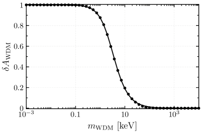
Figure 2: Relation between $\delta A_{\rm WDM}$ and ${m_{\rm WDM}}$. The point markers correspond to numerical results obtained through Eq. (14), while the solid curve corresponds to the best-fit parametrization in Eq. (15).

Equipped with a map between $\delta A_{\rm WDM}$ and ${m_{\rm WDM}}$, we may now identify $m_{\delta A}$ for a given dark-matter model as the value of ${m_{\rm WDM}}$ for which $\delta A=\delta A_{\rm WDM}$. Equivalently, given the value of $\delta A$ for our model, we can simply invert Eq. (15) to define

$$m_{\delta A}~{}\equiv~{}\left[\frac{(\delta A)^{-1/c}-1}{a}\right]^{1/b}~{}{\rm keV}~{}.$$ (16)

For any proposed model of dark-matter physics, we now have a recipe for calculating two mass scales, ${m_{1/2}}$ and $m_{\delta A}$, corresponding to the two different recast methods. Each of these is a continuous parameter which varies across the parameter space of a given dark-matter model and which quantifies how close to satisfying the Lyman-$\alpha$ bounds the different recast methods find the model to be. In other words, ${m_{1/2}}$ and $m_{\delta A}$ independently assess the viability of the proposed dark-matter model.

However, these variables not only permit us to construct Lyman-$\alpha$ constraints — they also permit us to compare our two recast methods in a quantitative manner by evaluating the quotient

$$R~{}\equiv~{}\frac{{m_{1/2}}}{m_{\delta A}}~{}.$$ (17)

Indeed, just like ${m_{1/2}}$ and $m_{\delta A}$, this comparator $R$ will generally also vary across the parameter space of a given dark-matter model. On the one hand, when $R\approx 1$, the two recasts are consistent with each other and provide similar results. On the other hand, when $R$ differs significantly from $1$, the recasts are inconsistent with each other. In this case, the choice of recast has a significant effect on the corresponding Lyman-$\alpha$ constraints, producing different exclusion regions for the same dark-matter model.

The questions we face, then, are two-fold. First, we would like to determine the sorts of general dark-matter models and associated parameter-space regions which are generally viable or excluded by Lyman-$\alpha$ constraints. At the same time, however, we also seek to determine for which classes of dark-matter models — and for which portions of their associated parameter spaces — we obtain $R\approx 1$, and for which classes of models and regions of associated parameter space we do not. It is to these questions that we now turn.

IV Lyman-$\alpha$ Constraints on Class-I Velocity Distributions

Our aim in this paper is to investigate the Lyman-$\alpha$ constraints on a multitude of possible dark-matter velocity distributions. In conducting this investigation, we shall proceed systematically, beginning with the simplest such distributions and then broadening the scope of our analysis to include more complicated, multi-modal ones. In this section, we shall begin by focusing on Class-I velocity distributions, including thermal distributions and distributions which can be approximated as Gaussian. We shall then expand our analysis to consider Class-II velocity distributions in Sect. V.

Before we proceed, however, we emphasize once again that a lack of complexity in the dark-matter velocity distribution does not necessarily reflect a corresponding lack of complexity in the particle content of the dark sector or in the interaction Lagrangian which governs the dynamics within that sector. Indeed, one can easily imagine complicated dark sectors which involve large numbers of particle species and/or non-trivial interactions, but which nevertheless yield dark-matter velocity distributions which are trivial in terms of their overall shapes.

IV.1 Thermal Distributions

In order to establish a baseline, we shall first consider velocity distributions similar to the canonical distribution which arises in WDM scenarios. Indeed, such velocity distributions can be expected to arise for dark-matter particles of mass $m$ which are initially in thermal equilibrium with a radiation bath, but subsequently decouple from that bath at a time prior to ${t_{\rm MRE}}$ when the bath temperature $T_{d}$ greatly exceeds $m$. The present-day phase-space distribution for such a dark-matter species is then given by the Maxwell-Boltzmann form

$$g(p)~{} =~{}\frac{1}{2}\,{\cal N}\left(\frac{p}{T_{d}a_{d}}\right)^{\!\!3}\exp\left[-p/(T_{d}a_{d})\right]\ ,$$ (18)

where we have ignored modifications due to Fermi/Bose statistics, where ${\cal N}$ is a normalization factor defined according to Eq. (2), and where $a_{d}$ denotes the value of the scale factor at $t_{d}$. The average momentum for a population of dark-matter particles with a phase-space distribution given by Eq. (18) is

$$\left\langle p\right\rangle~{}=~{}3T_{d}a_{d}\ .$$ (19)

This result implies that the $g(p)$ distribution in Eq. (18) is completely specified by $\left\langle p\right\rangle$ and can be viewed as a function of the ratio $p/\left\langle p\right\rangle$.

It is well known that $\left\langle p\right\rangle$ plays a crucial role in determining how cosmological perturbations grow in scenarios with $g(p)$ distributions of this sort. Indeed, as indicated in Eq. (4), $\left\langle v\right\rangle\approx\left\langle p\right\rangle/m$ effectively sets the free-streaming horizon for the dark matter and thereby the wavenumber $k_{\rm FSH}$ above which $P(k)$ is suppressed. However, the shape of the distribution can also be important [6, 37], particularly if the higher moments of the distribution — such as the standard deviation or the skewness — are large.

For the phase-space distribution in Eq. (18), we observe that these higher moments are all independent of $\left\langle p\right\rangle$. Indeed, this is related to the fact that a change in the value of $\left\langle p\right\rangle$ does not affect the shape of this distribution in $\log p$-space, but instead merely shifts it uniformly to higher or lower values of $\log p$. For example, the standard deviation of $\log p$ for this distribution turns out to be

$$\sigma~{} \equiv~{}\sqrt{\langle(\log p-\langle\log p\rangle)^{2}\rangle}$$

$$=~{}\sqrt{\frac{\pi^{2}}{6}-\frac{5}{4}}~{}\approx~{}0.63\ .$$ (20)

Likewise, the skewness for this distribution is

$$S~{} \equiv~{}\frac{\langle(\log p-\langle\log p\rangle)^{3}\rangle}{\sigma^{3}}$$

$$=~{}\frac{\frac{9}{4}-2\zeta(3)}{\left(\frac{\pi^{2}}{6}-\frac{5}{4}\right)^{3/2}}~{}\approx~{}-0.62\ .$$ (21)

The negative value of $S$ indicates that the distribution “tilts” to the right as compared with one which would have been perfectly symmetric in $\log\,p$-space.

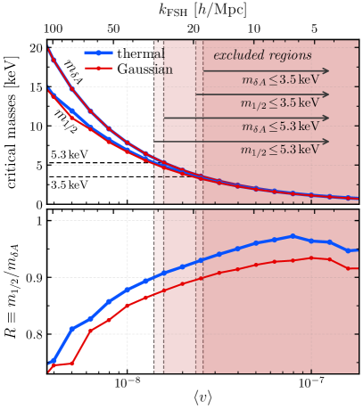
Figure 3: The critical masses ${m_{1/2}}$ and $m_{\delta A}$ (upper panel) and the comparator $R$ (lower panel), plotted as functions of $\left\langle v\right\rangle$ for the thermal velocity distribution in Eq. (18) and the Gaussian velocity distribution to be discussed in Eq. (22), the latter with a width $\sigma=0.63$ taken to match that of the thermal distribution. Also shown are the Lyman-$\alpha$ exclusion regions for the thermal velocity distribution according to our half-mode and $\delta A$ recasts for the critical masses $3.5$ keV and $5.3$ keV. The top axis indicates the dark-matter free-streaming horizon wavenumber $k_{\rm FSH}$ corresponding to each value of $\left\langle v\right\rangle$. We observe that within the observationally viable regions of $\left\langle v\right\rangle$, the comparator $R$ departs considerably from unity, indicating a meaningful disagreement between the results of the two recasts.

We now seek to assess for which velocities $\left\langle v\right\rangle$ the Lyman-$\alpha$ constraints can be satisfied, given the distribution in Eq. (18). In order to do this, we evaluate the transfer function $T^{2}(k)$ which corresponds to the dark-matter distribution $g(p)$ for many different values of $\left\langle v\right\rangle$. We then employ the recasts from Sect. III in order to obtain information about the Lyman-$\alpha$ bounds.

In the upper panel of Fig. 3, we plot the critical masses ${m_{1/2}}$ and $m_{\delta A}$ (blue curves) for the dark-matter phase-space distribution in Eq. (18) as functions of $\left\langle v\right\rangle$. In the lower panel of this same figure, we plot the corresponding value of the comparator $R\equiv{m_{1/2}}/m_{\delta A}$ (red curve). Since the relation between $\left\langle v\right\rangle$ and the free-streaming horizon in Eq. (4) establishes a one-to-one correspondence between values of $\left\langle v\right\rangle$ and values of the comoving wavenumber $k_{\rm FSH}$ for Class-I velocity distributions such as this one, tick marks indicating the values $k_{\rm FSH}$ have also been included at the top of each panel.

We immediately see from Fig. 3 that while ${m_{1/2}}$ and $m_{\delta A}$ agree quite well for large $\left\langle v\right\rangle$, a significant difference between them begins to develop as $\left\langle v\right\rangle$ decreases. As a result of this difference, the constraints on $\left\langle v\right\rangle$ obtained from each of the two recasts differ. Indeed, when we employ the less conservative bound ${m_{\rm WDM}}\gtrsim 3.5\,{\rm keV}$ in implementing each recast, we find that the half-mode analysis excludes the light-gray region on the right side of the figure, while the $\delta A$ analysis also excludes the thin, dark-gray stripe. Likewise, if we employ the more conservative bound ${m_{\rm WDM}}\gtrsim 5.3\,{\rm keV}$, we find that the half-mode analysis further excludes the dark-red region, while the $dA$ analysis also excludes the thin, light-red stripe.

While these differences are not terribly significant, we observe that the difference between ${m_{1/2}}$ and $m_{\delta A}$ becomes more and more pronounced as $\left\langle v\right\rangle$ decreases. Indeed, we observe that the comparator falls to $R\approx 0.72$ at the left edge of Fig. 3. That such a difference between recast predictions can arise even for the case of a simple, Class-I velocity distribution suggests that significantly smaller $R$ values could arise for other, more complicated distributions. As we shall see, this indeed turns out to be the case.

IV.2 Gaussian Distributions

The thermal dark-matter phase-space distribution in Eq. (18) provides a well-motivated and simple baseline from which to begin our exploration of more general functional forms of $g(p)$. However, since the parameters characterizing the shape of this baseline distribution — i.e., its width $\sigma$, its skewness $S$, etc.— were completely specified, our analysis thus far has exposed the sensitivity of the Lyman-$\alpha$ constraints to a single variable only, namely the average velocity $\left\langle v\right\rangle$.

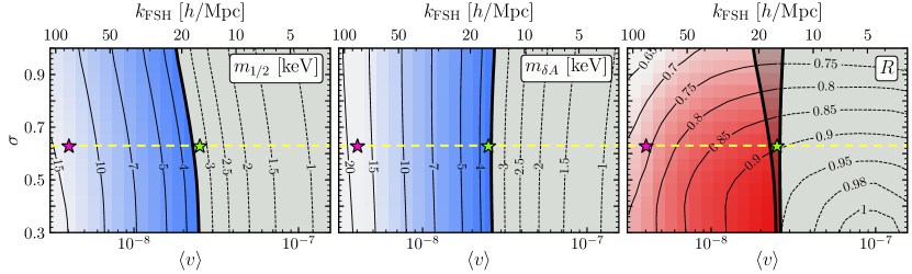
Figure 4: Contours in the $(\left\langle v\right\rangle,\sigma)$-plane of the critical masses ${m_{1/2}}$ (left panel) and $m_{\delta A}$ (center panel), as well as the comparator $R$ (right panel), for the Gaussian phase-space distribution in Eq. (22). The thick black curves in the left and center panels indicate the Lyman-$\alpha$ constraint obtained by employing the less conservative bound ${m_{\rm WDM}}\gtrsim 3.5\,{\rm keV}$ when implementing the corresponding recast. The gray region to the right of each thick black curve is excluded. The exclusion contours for both of these recasts are also superimposed on the contours of $R$ shown in the right panel. The dashed yellow line in each panel corresponds to $\sigma=0.63$, which matches the standard deviation of the distribution in Eq. (18). The magenta and green stars indicate the locations in the $(\left\langle v\right\rangle,\sigma)$-plane for which the corresponding transfer functions are plotted in Fig. 5.

We would now like to extend our study and examine how variations in the shape of a unimodal distribution modify the Lyman-$\alpha$ constraints. To this end, we shall now consider the case in which $g(p)$ takes the form of a Gaussian distribution in $(\log\,p)$-space:

$$g(p)~{} =~{}\frac{{\cal N}}{\sqrt{2\pi\sigma^{2}}}\exp\left[-\frac{(\log p-\langle\log p\rangle)^{2}}{2\sigma^{2}}\right]\ ,$$ (22)

where we take the mean $\langle\log p\rangle$ and standard deviation $\sigma$ to be free parameters, and where ${\cal N}$ is a normalization factor. We note that for a log-normal distribution of this sort we may also express $\left\langle\log p\right\rangle$ in terms of $\left\langle p\right\rangle$ — or, equivalently, in terms of $\left\langle v\right\rangle\approx\left\langle p\right\rangle\!/m$ — through the relation $\langle\log p\rangle=\log\langle p\rangle-\sigma^{2}/2$. This relation will allow us to compare the results we obtain for this phase-space distribution directly with those obtained from the baseline thermal distribution in Eq. (18).

We shall begin our analysis of the phase-space distribution in Eq. (22) by considering how the difference in shape between this distribution and the baseline thermal distribution in Eq. (18) affects our results for ${m_{1/2}}$ and $m_{\delta A}$. In order to facilitate a direct comparison between these two distributions, we fix the standard deviation for our Gaussian to the value $\sigma=0.63$ which accords with Eq. (20) and examine how these two critical masses behave as functions of $\left\langle v\right\rangle$. Our results for ${m_{1/2}}$ and $m_{\delta A}$ are indicated by the red curves in the upper panel of Fig. 3, while the corresponding results for $R$ are indicated by the red curve in the lower panel. The $m_{\delta A}$ curve for the Gaussian distribution coincides almost exactly with the corresponding curve for the baseline thermal distribution in Eq. (18) — so much so, in fact, that it is effectively hidden beneath that curve. By contrast, the ${m_{1/2}}$ curve for the Gaussian distribution departs appreciably from the corresponding curve for the baseline distribution, and the value of $R$ is consequently smaller for the Gaussian. These results indicate that even for unimodal, Class-I velocity distributions, the shape of the distribution can have a small but appreciable impact on the results obtained from the half-mode recast. Nevertheless, we do not find a particularly large difference between the Lyman-$\alpha$ bounds obtained for these two distributions.

We now expand our analysis of the phase-space distribution in Eq. (22) in order to examine the effect of varying $\sigma$ as well as $\left\langle v\right\rangle$. Indeed, by varying $\sigma$ as well as $\left\langle v\right\rangle$ , we are now actually varying the shape of the log-normal distribution in Eq. (22) and not merely shifting this distribution rigidly along the $(\log\,p)$-axis. In Fig. 4, we display contours of ${m_{1/2}}$ (left panel) and $m_{\delta A}$ (center panel) in $(\left\langle v\right\rangle,\sigma)$-space for the velocity distribution in Eq. (22). The thick black curve in each of these two panels panel shows the Lyman-$\alpha$ bound obtained by employing the less conservative bound ${m_{\rm WDM}}\gtrsim 3.5\,{\rm keV}$ in implementing the corresponding recast. The gray region to the right of each each thick black curve is excluded. In the right panel of the figure, the exclusion contours for both of these recasts are superimposed on the contours of the comparator $R$. For $\sigma=0.63$ (yellow line shown in each panel), the results obtained for ${m_{1/2}}$ and $m_{\delta A}$ correspond to those plotted in Fig. 3.

Once again, we observe that while there are regions of parameter space wherein the results of the half-mode and $\delta A$ recasts coincide quite well, there are other regions — especially those within which $\left\langle v\right\rangle$ is small or $\sigma$ is large — wherein $R$ differs significantly from unity. The results shown in the left panel indicate that the constraint derived from the half-mode recast tightens by roughly $30\%$ over the region of parameter space shown as $\sigma$ increases and $g(p)$ becomes broader. Ultimately, this stems from the fact that a broader phase-space distribution includes a non-negligible population of dark-matter particles at higher velocities that can smooth out structure on larger scales. As a result, ${m_{1/2}}$ decreases as $\sigma$ increases, leading to more stringent constraints on models with broader $g(p)$ distributions. By contrast, the results shown in the center panel of Fig. 4 indicate that the constraint derived from the $m_{\delta A}$ recast does not depend sensitively on the value of $\sigma$. Indeed, across the range of $\sigma$ shown, this constraint is approximately the same as that obtained for our baseline thermal distribution in Eq. (18).

The results for $R$ displayed in the right panel of Fig. 4 indicate that the half-mode and $\delta A$ recasts yield similar bounds when $\sigma$ is relatively small. However, for $\sigma\gtrsim 0.5$, the constraints obtained from the two recasts diverge, with $R$ deviating significantly from unity across the upper portions of the panel. Furthermore, the results for $R$ within the region of $(\left\langle v\right\rangle,\sigma)$-space which is not currently excluded by Lyman-$\alpha$ data indicate how the Lyman-$\alpha$ constraints would change if future observations were to further tighten the Lyman-$\alpha$ bound on ${m_{\rm WDM}}$. In particular, we find that the disagreement between recasts becomes more severe as $\left\langle v\right\rangle$ decreases and as $\sigma$ increases.

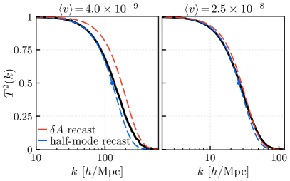
Figure 5: The transfer functions $T^{2}(k)$ which correspond to the parameter-space points indicated by the magenta and green stars in Fig. 4. The results in the left panel correspond to the magenta star, which is situated within a region of parameter space which lies far from the exclusion region and for which the value of $R$ is relatively small, while the results in the right panel correspond to the green star, which is situated near the Lyman-$\alpha$ exclusion contours associated with both recasts. The solid black curve in each panel represents the result of a numerical calculation, while the dashed curves represent the WDM transfer functions onto which this $T^{2}(k)$ is effectively mapped by the half-mode and $\delta A$ recasts.

The results shown in Fig. 4 beg the question whether an even more dramatic departure from the results obtained for our baseline thermal distribution in Eq. (18) would be obtained for Gaussian $g(p)$ distributions with even larger values of $\sigma$. Unfortunately, within this region of parameter space — particularly for small values of $\left\langle v\right\rangle$ — assessing the values of ${m_{1/2}}$ and $m_{\delta A}$ becomes challenging in practice, as the simulations required to evaluate $T^{2}(k)$ become significantly more computationally expensive. Nevertheless, based on our qualitative understanding of how the bounds obtained from the ${m_{1/2}}$ and $m_{\delta A}$ recasts arise, we would expect that the bounds obtained from both recasts become significantly tighter when $\sigma$ becomes increasingly large.

Further insight into the results shown in Fig. 4 can be gleaned from examining how the shape of the transfer function itself varies across $(\left\langle v\right\rangle,\sigma)$-space. In Fig. 5, we show the numerical results for $T^{2}(k)$ (solid black curves) for two different points within that parameter space. The curve in the left panel corresponds to the point $(\left\langle v\right\rangle,\sigma)=(4\times 10^{-9},0.63)$ indicated by the magenta star in Fig. 4, while the curve in the right panel corresponds to the point $(\left\langle v\right\rangle,\sigma)=(2.5\times 10^{-8},0.63)$ indicated by the green star. In each panel, alongside the true $T^{2}(k)$ curve obtained for the Gaussian $g(p)$ distribution in question, we also plot the $T^{2}(k)$ curves obtained for WDM models with ${m_{\rm WDM}}$ set equal to the value of ${m_{1/2}}$ (dashed blue curve) and $m_{\delta A}$ (dashed red curve) that we obtain for this $g(p)$ distribution. In other words, these dashed blue and red curves respectively represent the WDM transfer functions onto which the true $T^{2}(k)$ is effectively mapped by the half-mode and $\delta A$ recasts.

We see from the right panel of Fig. 5 that the $T^{2}(k)$ curves associated with both recasts nearly coincide both with each other and with the true $T^{2}(k)$ curve obtained for this parameter-space point. Indeed, this result is not unexpected, given that $R\approx 0.90$ is reasonably close to unity for this point, which lies very close to the Lyman-$\alpha$ exclusion contours in Fig. 4 associated with both recasts. By contrast, for the point shown in the left panel, not only do the WDM transfer functions associated with these two recasts differ appreciably from each other, they also both differ appreciably from the true $T^{2}(k)$ curve. Again, this is not unexpected, given that $R\approx 0.74$ differs significantly from unity for this point. However, the results shown in this panel illustrate the ways in which these recasts can yield unreliable results when the shape of the dark-matter velocity distribution differs from that of WDM.  Moreover, they also illustrate how sensitively the Lyman-$\alpha$ constraints depend on the precise form of $T^{2}(k)$. Indeed, as we shall now see, these issues can become even more pronounced for Class-II distributions.

V Lyman-$\alpha$ Constraints on Class-II Velocity Distributions

We now expand our analysis to include a broader variety of dark-matter velocity distributions — distributions which depart more dramatically from the simple, unimodal Class-I distributions we have considered thus far. One particularly interesting possibility along these lines is to consider distributions which are multi-modal. Indeed, Class-II distributions of this sort arise in a variety of dark-matter scenarios in which non-negligible contributions to the dark-matter abundance occur at different timescales. Such scenarios include those in which freeze-out or freeze-in [7, 38, 39] production is accompanied by production from the out-of-equilibrium decays of heavy particles at late times; those in which different decay channels for the same unstable particle species with different decay kinematics contribute non-negligibly to the dark-matter abundance [8]; and those in which dark-matter is produced non-thermally through decay cascades [6].

In order to examine multi-modal velocity distributions of this sort, we shall consider a phase-space distribution $g(p)$ which consists of a sum of Gaussian peaks, each of which takes the form specified in Eq. (22) and each of which provides a contribution $\Omega_{i}$ toward the total present-day dark-matter abundance $\Omega\equiv\sum_{i}\Omega_{i}\approx 0.26$ [1]. Such a form for $g(p)$ is indeed nothing but a Gaussian decomposition of the phase-space distribution in $\log p$-space, and as such is capable of approximating most distributions of interest. We shall parametrize this phase-space distribution as follows:

$$g(p)~{}\approx~{}\!\!\!\sum_{i=0}^{N_{G}-1}\!\!\frac{\mathcal{N}\Omega_{i}}{\sqrt{2\pi}\sigma_{i}\Omega}\!\exp\left\{\!-\frac{1}{2\sigma^{2}_{i}}\left[\log\left(\!\frac{p}{\langle p\rangle_{i}}\!\right)+\frac{1}{2}\sigma^{2}_{i}\right]^{2}\!\right\}\ ,$$ (23)

where $\left\langle p\right\rangle_{i}$ is the average momentum of the $i^{\,\rm th}$ Gaussian, where $\sigma_{i}$ is the corresponding width, where $N_{G}$ is the number of Gaussian components included in the sum, and where the index $i=0,1,2,\ldots,N_{G}-1$ labels these components in order of decreasing $\left\langle p\right\rangle_{i}$.

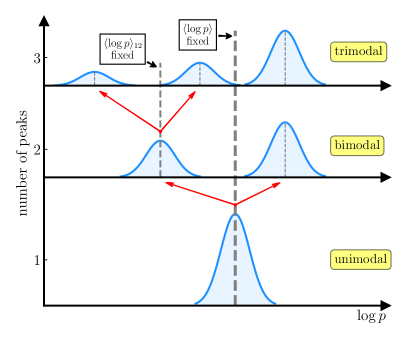
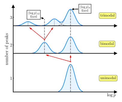
Figure 6: Two schematics illustrating methods through which multi-modal dark-matter velocity distributions can be generated from a single unimodal distribution. Left panel: The lowest-velocity peak at each step is bifurcated into two peaks in such a manner as to preserve the “center of velocity” $\left<\log p\right>_{ij}$ defined in Eq. (24) for the two-peak system, while keeping $\left<\log p\right>$ fixed. Right panel: Here the bifurcation procedure keeps both $\left<\log p\right>_{ij}$ and $\left<\log p\right>_{0}$ fixed. The analysis to be discussed in Sects. V.1 and V.2 is based on this approach.

Since a $g(p)$ distribution of this form with $N_{G}$ Gaussian components is described by $3N_{G}-1$ free parameters, systematically surveying the parameter space of possible $g(p)$ distributions rapidly becomes impractical as $N_{G}$ increases. It will therefore be necessary for us to impose certain simplifying assumptions if we wish to explore the landscape of possible $g(p)$ distributions of the form given in Eq. (23) in a meaningful yet tractable way. One of our principal aims in this paper is to assess how the detailed shape of a particular feature in $g(p)$ — not merely the average velocity of the particles associated with that feature, but the full distribution of velocities — affects the results of the half-mode and $\delta A$ recasts. Whatever procedure we adopt should further this aim to whatever extent possible and highlight the ways in which the detailed shape of $g(p)$ impacts the Lyman-$\alpha$ constraints derived from the half-mode and $\delta A$ recasts.

An analysis procedure which furthers this aim is illustrated schematically in the left panel of Fig. 6. According to this procedure, one begins with a $g(p)$ distribution consisting of a single Gaussian peak with a specified width $\sigma_{0}$ and average velocity $\left\langle v\right\rangle_{0}$. One then splits this peak into two individual peaks whose individual widths $\sigma_{0}$ and $\sigma_{1}$ are each equal to the width of the original peak and whose total abundance $\Omega_{0}+\Omega_{1}$ is equal to the abundance of the original peak. Next, one separates these new peaks in velocity-space by endowing them with different average velocities $\left\langle v\right\rangle_{0}$ and $\left\langle v\right\rangle_{1}$. However, one does this in such a way that the abundance-weighted “center of velocity” $\left\langle\log v\right\rangle_{01}$ for these peaks — a quantity which we define as

$$\left\langle\log v\right\rangle_{ij}~{}\equiv~{}\frac{\Omega_{i}}{\Omega_{i}+\Omega_{j}}\!\left\langle\log v\right\rangle_{i}+\frac{\Omega_{j}}{\Omega_{i}+\Omega_{j}}\!\left\langle\log v\right\rangle_{j}$$ (24)

for any two peaks labeled by indices $i$ and $j$ — remains equal to the center of velocity of the original peak. One may then iterate this procedure by taking the lowest-velocity peak in the resulting distribution, splitting it into two peaks whose individual widths $\sigma_{1}$ and $\sigma_{2}$, total abundance $\Omega_{1}+\Omega_{2}$, and center of velocity $\left\langle\log v\right\rangle_{12}$ are equal to the abundance and center of velocity of that original peak, and so forth. In this procedure, $\left<\log p\right>$ remains fixed for the total population of dark-matter components.

This iterative procedure has several features. First, each time we perform such a bifurcation, we introduce only two additional free parameters: one which characterizes the relative abundances of the two resulting peaks and one which characterizes their separation in $(\log p)$-space. Second, since the shape of the matter power spectrum is quite sensitive to small modifications of $g(p)$ at large $p$, it is useful to adopt a procedure in which one examines the effect of modifying the shape of $g(p)$ of small $p$ while leaving the structure at large $p$ fixed. Third, since we hold the center of velocity fixed when we perform this bifurcation, any difference between the Lyman-$\alpha$ constraints that we obtain for the resulting $g(p)$ distribution relative to the original distribution is solely a consequence of the differences in their detailed shapes.

More mathematically, we can understand this approach as follows. Like any distribution function, $g(p)$ can be described in terms of its moments. The zeroth moment of any distribution is the total area under the curve. For $g(p)$, this is the total dark-matter abundance, which we are holding fixed. The first moment of any distribution is then the average value of its independent variable — in this case, the average velocity $\langle\log v\rangle_{ij}$. Holding this quantity fixed therefore enables us to disentangle the effects of these first two moments of $g(p)$ on the Lyman-$\alpha$ constraints, and thereby isolate the dependence of the Lyman-$\alpha$ constraints on the higher moments of the distribution which concern the distribution of the dark-matter velocities around this average velocity. Indeed, in some sense this has been the goal of our study all along, given that Class I and Class II distributions differ in precisely how these velocities are distributed relative to the mean.

This procedure, although mathematically elegant, is computationally difficult to realize in practice. However, we may follow a slightly modified version of this procedure which is also capable of surveying phenomenologically rich portions of the multi-modal parameter space. This alternative procedure is shown in the right panel of Fig. 6. As before, one begins with a $g(p)$ distribution consisting of a single Gaussian peak with a width $\sigma_{0}$ and average velocity $\left\langle v\right\rangle_{0}$, and splits it into two peaks. However, instead of holding the center of velocity of the system fixed, one holds $\left<\log v\right>_{0}$ fixed and fission off some of the abundance of this peak in order to construct a second peak with average velocity $\left<\log v\right>_{1}<\left<\log v\right>_{0}$. One then proceeds by bifurcating this colder peak in the same way that one would have done it in the original procedure, by holding $\left<\log v\right>_{12}$ fixed, and so forth. This modified procedure allows us examine the impact of the lower-velocity peak on the Lyman-$\alpha$ constraints for the $N_{G}=2$ case in a more straightforward manner. In what follows, we adopt the procedure outlined in the right panel in our analysis.

V.1 Bi-Modal Distributions

We begin our analysis of the Lyman-$\alpha$ constraints on phase-space distributions of the general form in Eq. (23) by considering the simplest non-trivial case — the case of distributions with $N_{G}=2$ Gaussian components. For simplicity, in exploring the five-dimensional parameter space which characterizes these double-peak $g(p)$ distributions, we shall set the widths of the two Gaussian components to be equal to each other and focus on the effects of varying the average velocity $\left\langle v\right\rangle_{0}\approx\left\langle p\right\rangle_{0}/m$ associated with the highest-momentum component, the fractional abundance contribution $\Omega_{0}/\Omega$ associated with this same component, and the ratio $\left\langle v\right\rangle_{1}/\left\langle v\right\rangle_{0}\approx\left\langle p\right\rangle_{1}/\left\langle p\right\rangle_{0}<1$ of the average velocities of the two components. Moreover, we shall take $\sigma_{0}=\sigma_{1}=0.63$, such that these widths accord with the standard deviation of $\log p$ for our baseline velocity distribution in Eq. (18).

In Fig. 7, we show three examples of double-peak $g(p)$ distributions, all with $\left\langle v\right\rangle_{0}=8.0\times 10^{-7}$ and $\left\langle v\right\rangle_{1}/\left\langle v\right\rangle_{0}=1.3\times 10^{-2}$, but with different values of $\Omega_{0}/\Omega$. We plot these distributions as functions of $p/m$. In order to provide a sense of how different parts of these $g(p)$ distributions impact structure formation, we also associate a wavenumber $k$ with each value of $p/m$. This wavenumber, which is indicated on the top axis of the figure, effectively represents the value of $k$ above which a population of dark-matter particles all moving at exactly the same speed $v\approx p/m$ contributes to the suppression of $P(k)$ through free-streaming, according to Eq. (4). The dashed green vertical lines indicate the values of ${k_{1/2}}$ which correspond to the WDM masses ${m_{\rm WDM}}=3.5~{}{\rm keV}$ and ${m_{\rm WDM}}=5.3~{}{\rm keV}$. The Lyman-$\alpha$ constraint derived from the half-mode recast for either of these ${m_{\rm WDM}}$ values is sensitive to the detailed shape of $g(p)$ in the region of the plot to the right of the corresponding ${k_{1/2}}$ line. By contrast, the dashed brown vertical lines in the figure delimit the range of wavenumbers $k_{\rm min}\leq k\leq k_{\rm max}$ over which the averaging is performed in Eq. (12) in order to obtain $\delta A$. The Lyman-$\alpha$ constraint derived from the $\delta A$ recast is sensitive to the detailed of $g(p)$ in the region to the left of the $k_{\rm min}$ line.

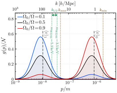
Figure 7: Three $g(p)$ distributions of the general form specified in Eq. (23), each of which is a superposition of $N_{G}=2$ Gaussian peaks. The average momenta $\left\langle p\right\rangle_{0}$ and $\left\langle p\right\rangle_{1}$ associated with these two peaks are the same for all three distributions, but the fractional abundance $\Omega_{0}/\Omega$ associated with the higher-momentum peak is different for each one. The value of $k$ above which the dark-matter particles in $g(p)$ with velocity $p/m$ can suppress power due to free-streaming effects is indicated along the top axis. The dashed brown vertical lines indicate the wavenumbers $k_{\rm min}$ and $k_{\rm max}$ which delimit the range of $k$ values over which the averaging is performed in Eq. (12) in order to obtain $\delta A$. The dashed green vertical lines indicate the values of ${k_{1/2}}$ which correspond to the WDM masses ${m_{\rm WDM}}=3.5~{}{\rm keV}$ and ${m_{\rm WDM}}=5.3~{}{\rm keV}$.

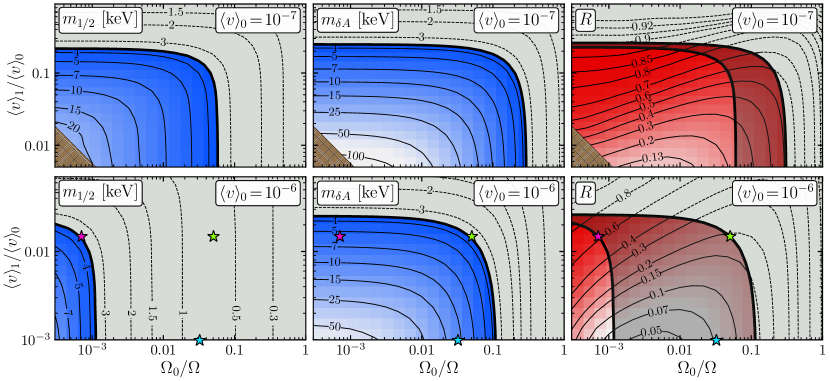
Figure 8: Contours in the $(\Omega_{0}/\Omega,\left\langle v\right\rangle_{1}/\left\langle v\right\rangle_{0})$-plane of ${m_{1/2}}$ (left panel of each row) and $m_{\delta A}$ (center panel), as well as the comparator $R$ (right panel), for the general phase-space distribution in Eq. (23) with $N_{G}=2$. The results shown in the top and bottom rows respectively correspond to the choices $\left\langle v\right\rangle_{0}=10^{-7}$ and $\left\langle v\right\rangle_{0}=10^{-6}$ for the average velocity of the higher-velocity Gaussian peak, while the widths of both peaks have been set to $\sigma_{0}=\sigma_{1}=0.63$ in all panels. As in Fig. 4, the thick black curve in the left and center panels of each row indicates the Lyman-$\alpha$ constraint obtained by employing the bound ${m_{\rm WDM}}\gtrsim 3.5\,{\rm keV}$ in implementing the corresponding recast. The gray region above and to the right of each thick black curve is excluded. The exclusion contours for both of these recasts are superimposed on the contours of $R$ shown in the right panel. The magenta and green stars indicate the combinations of $\Omega_{0}/\Omega$ and $\left\langle v\right\rangle_{1}/\left\langle v\right\rangle_{0}$ for which the transfer functions are plotted in Figs. 9 and 12. The blue star indicates an additional combination of $\Omega_{0}/\Omega$ and $\left\langle v\right\rangle_{1}/\left\langle v\right\rangle_{0}$ for which the transfer function is also plotted in Fig. 12. Within the brown cross-hatched regions of the panels in the upper row, $g(p)$ is consistent with Lyman-$\alpha$ constraints, but the values of ${m_{1/2}}$ and $m_{\delta A}$ could not both be reliably determined numerically to the desired accuracy.

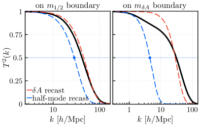
Figure 9: The transfer functions $T^{2}(k)$ which correspond to the parameter-space points indicated by the magenta and green stars in Fig. 8. The results in the left panel correspond to the magenta star, which is situated on the Lyman-$\alpha$ exclusion contour obtained from the half-mode recast, while the results in the right panel correspond to the green star, which is situated on the Lyman-$\alpha$ exclusion contour obtained from the $\delta A$ recast. The solid black curve in each panel represents the result of a numerical calculation, while the dashed curves represent the WDM transfer functions onto which this $T^{2}(k)$ is effectively mapped by the half-mode and $\delta A$ recasts.

Proceeding as we did with the Class-I distributions that we examined in Sect. IV, we survey the parameter space of possible double-peak $g(p)$ distributions, evaluating the critical masses ${m_{1/2}}$ and $m_{\delta A}$ and the comparator $R$ at each point. The results of this analysis are shown in Fig. 8. In particular, we show contours of ${m_{1/2}}$ (left panel of each row), $m_{\delta A}$ (center panel), and $R$ (right panel) in the $(\Omega_{0}/\Omega,\left\langle v\right\rangle_{1}/\left\langle v\right\rangle_{0})$-plane for two different choices of $\left\langle v\right\rangle_{0}$. The results displayed in the top row correspond to the choice $\left\langle v\right\rangle_{0}=10^{-7}$, while those displayed in the bottom row correspond to the choice $\left\langle v\right\rangle_{0}=10^{-6}$. In both rows, we have fixed $\sigma_{0}=\sigma_{1}=0.63$. As in Fig. 4, the thick black curves in the left and center panels of each row of the figure indicate the Lyman-$\alpha$ constraints obtained by employing the bound ${m_{\rm WDM}}\gtrsim 3.5\,{\rm keV}$ in implementing the corresponding recast. The gray region above and to the right of each such curve is excluded. The exclusion contours for both of these recasts are superimposed on the contours of $R$ shown in the right panel of the corresponding row. Within the brown cross-hatched regions of the figure, $g(p)$ is consistent with Lyman-$\alpha$ constraints, but the values of ${m_{1/2}}$ and $m_{\delta A}$ could not both be reliably determined numerically to the desired accuracy.

The shapes of the exclusion contours in Fig. 8 reveal that Lyman-$\alpha$ data effectively impose two separate constraints on these double-peak $g(p)$ distributions. First, they place an upper bound on the abundance $\Omega_{0}$ associated with the higher-velocity peak. Second, they also place an upper bound on the average velocity $\left\langle v\right\rangle_{1}$ associated with the lower-velocity peak. The precise upper limit on each of these quantities depends on the value of $\left\langle v\right\rangle_{0}$. It is also worth noting that the entire right edge of each panel in the top row of the figure — an edge along which ${m_{1/2}}$ and $m_{\delta A}$ are both constant — corresponds to the single point along the dashed yellow line in Fig. 4 at which $\left\langle v\right\rangle_{0}=10^{-7}$.

More striking, however, is the disagreement between the results derived from the half-mode and $\delta A$ recasts for Class-II velocity distributions of this sort. For $\langle v\rangle_{0}=10^{-7}$, the exclusion region obtained from the half-mode recast extends beyond the region obtained for the $\delta A$ recast by roughly a factor of five in the $\Omega_{0}/\Omega$ direction. For $\langle v\rangle_{0}=10^{-6}$, the difference can be over two orders of magnitude, and nearly the entire region of the $(\Omega_{0}/\Omega,\left\langle v\right\rangle_{1}/\left\langle v\right\rangle_{0})$-plane shown in the figure is excluded according to the ${m_{1/2}}$ recast. This disagreement is also reflected in the values of the comparator. We observe that the values of $R$ across a significant portion of the parameter space shown in Fig. 8 are quite extreme in comparison with any value of $R$ which we encountered for the Class-I velocity distributions in Sect. IV.  We also observe that $R$ is not a monotonic function of $\Omega_{0}/\Omega$, but rather falls, reaches a minimum, and then rises again as this parameter is varied along any line of constant $\left\langle v\right\rangle_{1}/\left\langle v\right\rangle_{0}$.

The results in Fig. 7 actually illustrate one way in which these disagreements can arise for Class-II distributions. The vast majority of the abundance associated with the high-velocity peak in the $g(p)$ distributions shown lies within the range of $p/m$ within which both the half-mode and $\delta A$ recasts are sensitive. However, the majority of the abundance associated with the low-velocity peak lies within the region to which the $\delta A$ recast is sensitive, but the half-mode recast is not. We might therefore anticipate disagreements between the recasts to arise in situations in which $\Omega_{0}$ and $\Omega_{1}$ are both sizable.

Another way to understand the origin of the disagreement between these two recasts is to consider how the shape of $T^{2}(k)$ varies across our parameter space. In Fig. 9, we show the numerical results for $T^{2}(k)$ (solid black curves) for two different points within that space. The curve in the left panel corresponds to the point $(\Omega_{0}/\Omega,\left\langle v\right\rangle_{1}/\left\langle v\right\rangle_{0})\approx(7.0\times 10^{-4},0.015)$ indicated by the magenta star in Fig. 8, while the curve in the right panel corresponds to the point $(\Omega_{0}/\Omega,\left\langle v\right\rangle_{1}/\left\langle v\right\rangle_{0})\approx(4.8\times 10^{-2},0.015)$ indicated by the green star. In each panel, alongside the true $T^{2}(k)$ curve we also plot the $T^{2}(k)$ curves obtained for WDM models with ${m_{\rm WDM}}$ set equal to the corresponding value of ${m_{1/2}}$ (dashed blue curve) or $m_{\delta A}$ (dashed red curve).

The true $T^{2}(k)$ curve shown in the left panel of Fig. 9 represents a relatively mild but nevertheless meaningful departure from the transfer functions to which the Class-I distributions that we examined in Sect. IV give rise. The free-streaming of dark-matter particles associated with the higher-velocity peak leads to a suppression of power at lower $k$. Since $\Omega_{0}/\Omega\approx 7.0\times 10^{-4}$ is quite small in this case, this suppression is barely discernible to the eye. Nevertheless, it has a non-negligible impact on ${m_{1/2}}$, which is quite sensitive to the behavior of $T^{2}(k)$ at low $k$. By contrast, $m_{\delta A}$ is far less sensitive to such behavior, and the corresponding WDM transfer function accords reasonably well with the true form of $T^{2}(k)$. As a result, a disagreement arises between the values of ${m_{1/2}}$ and $m_{\delta A}$.

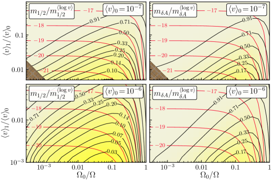
Figure 10: The effect of the detailed shape of $g(p)$ on the critical masses ${m_{1/2}}$ and $m_{\delta A}$. The left panel of each row shows contours (black curves) in the $(\Omega_{0}/\Omega,\left\langle v\right\rangle_{1}/\left\langle v\right\rangle_{0})$-plane of the ratio $m_{1/2}/m_{1/2}^{\langle\log v\rangle}$ of the half-mode mass obtained for a $g(p)$ distribution of the form in Eq. (23) with $N_{G}=2$ and $\sigma_{0}=\sigma_{1}=0.63$ to the half-mode mass obtained for the $g(p)$ distribution with $N_{G}=1$ and $\sigma_{0}=0.63$ which has the same value of $\langle\log v\rangle$. In the right panel of each row, we show contours of the corresponding ratio $m_{\delta A}/m_{\delta A}^{\langle\log v\rangle}$ for the other critical mass. Contours (red curves) of $\langle\log v\rangle$ itself are also included in each panel. The results shown in the top and bottom rows correspond to the choices $\left\langle v\right\rangle_{0}=10^{-7}$ and $\left\langle v\right\rangle_{0}=10^{-6}$, respectively. We observe that $m_{1/2}/m_{1/2}^{\langle\log v\rangle}$ and $m_{\delta A}/m_{\delta A}^{\langle\log v\rangle}$ can each differ significantly from unity, even within the region parameter space which is consistent with the corresponding exclusion contour in Fig. 8.

The true $T^{2}(k)$ curve shown in the right panel represents an even more dramatic departure from the transfer functions to which Class-I velocity distributions give rise. The abundance associated with the higher-velocity peak is significantly larger in this case, and the free-streaming of dark-matter particles associated with this peak has a more pronounced effect on $T^{2}(k)$ at lower $k$. As a result, the value of ${m_{1/2}}$ is comparatively low. However, since the lower-velocity peak carries the vast majority of the overall dark-matter abundance, $T^{2}(k)$ initially decreases only gradually with increasing $k$. Indeed, it is only at substantially higher values of $k$ that the free-streaming of the dark-matter particles associated with the low-velocity peak contributes to the suppression of structure and induces a precipitous drop in $T^{2}(k)$. As a result, the value of $m_{\delta A}$ is comparatively high, and a significant disagreement arises between the results of our two recasts.

Fig. 8, especially when supplemented by Fig. 9, reveals a great deal of information about the way in which the results of the half-mode and $\delta A$ recasts are modified by the presence of an additional Gaussian peak in $g(p)$. However, since the center of velocity $\left\langle\log v\right\rangle_{01}$ for $g(p)$ in the $N_{G}=2$ case depends on both $\left\langle v\right\rangle_{1}/\left\langle v\right\rangle_{0}$ and $\Omega_{0}/\Omega$, this figure does not reveal to what extent the variation of ${m_{1/2}}$ and $\delta A$ across the parameter space shown is simply a consequence of the variation in $\left\langle\log v\right\rangle_{01}$ and to what extent it is in fact a consequence of variations in the detailed shape of $g(p)$. As such, in Fig. 10, we provide additional information which illustrates how the detailed shape of $g(p)$ affects our results for these critical masses across the same region of the $(\Omega_{0}/\Omega,\left\langle v\right\rangle_{1}/\left\langle v\right\rangle_{0})$-plane shown in Fig. 8. In the left panel of Fig. 10, we show contours (black curves) of the ratio $m_{1/2}/m_{1/2}^{\langle\log v\rangle}$ of the half-mode mass obtained for the resulting $g(p)$ distribution to the half-mode mass obtained for the $g(p)$ distribution with $N_{G}=1$ and $\sigma_{0}=0.63$ which has the same center of velocity. In the right panel of each row, we show contours of the corresponding ratio $m_{\delta A}/m_{\delta A}^{\langle\log v\rangle}$ for the other critical mass. In each panel of the figure, we also show contours (red curves) of the center of velocity $\left\langle\log v\right\rangle_{01}$ itself.

The ratios $m_{1/2}/m_{1/2}^{\langle\log v\rangle}$ and $m_{\delta A}/m_{\delta A}^{\langle\log v\rangle}$ characterize the impact that the detailed shape of $g(p)$ has on the results of the two recasts. When either of these ratios departs significantly from unity, the result obtained from the corresponding recast differs significantly from the naïve result that one would obtain from a Class-I distribution with the same center of velocity. We see from Fig. 10 that indeed both ratios depart significantly from unity across large regions of the $(\Omega_{0}/\Omega,\left\langle v\right\rangle_{1}/\left\langle v\right\rangle_{0})$-plane. The most significant departures occur when $\left\langle v\right\rangle_{1}/\left\langle v\right\rangle_{0}$ is small and $\Omega_{0}/\Omega$ is $\mathcal{O}(0.1)$.

We also observe that $m_{1/2}/m_{1/2}^{\langle\log v\rangle}$ and $m_{\delta A}/m_{\delta A}^{\langle\log v\rangle}$ are both less than unity throughout the entirety of the $(\Omega_{0}/\Omega,\left\langle v\right\rangle_{1}/\left\langle v\right\rangle_{0})$-plane. This is ultimately a reflection of the fact that the bimodal $g(p)$ distribution associated with each point in this plane can be viewed as a bifurcation of the unimodal $g(p)$ distribution to which it is being compared — a bifurcation of precisely the sort described in the procedure outlines at the beginning of this section. This bifurcation shifts some portion of the abundance associated with the original peak to higher $v$ and some portion to lower $v$. However, because ${m_{1/2}}$ and $m_{\delta A}$ are in general more sensitive to modifications of the dark-matter velocity distribution at high $v$ than at low $v$, this shift leads to a decrease in both critical-mass ratios. Moreover, as we observe from the figure, the smaller $\left\langle v\right\rangle_{1}/\left\langle v\right\rangle_{0}$ is for a given $\Omega_{0}/\Omega$, the more significant that decrease is. We note that this is due not to any decrease in these critical masses themselves — indeed, ${m_{1/2}}$ and $m_{\delta A}$ both actually increase as $\left\langle v\right\rangle_{1}/\left\langle v\right\rangle_{0}$ decreases, as is evident from Fig. 8 — but rather to the fact that the corresponding critical masses $m_{1/2}^{\langle\log v\rangle}$ and $m_{\delta A}^{\langle\log v\rangle}$ increase more quickly. We also note that the decrease in $m_{1/2}/m_{1/2}^{\langle\log v\rangle}$ for a given set of model parameters is typically more extreme than the decrease in $m_{\delta A}/m_{\delta A}^{\langle\log v\rangle}$, owing to the fact that $m_{1/2}$ is more sensitive to small changes in the dark-matter velocity distribution at high $v$ than $m_{\delta A}$ is.

We remark that in defining the ratios $m_{1/2}/m_{1/2}^{\langle\log v\rangle}$ and $m_{\delta A}/m_{\delta A}^{\langle\log v\rangle}$ for a given $g(p)$ distribution with $N_{G}=2$, we have taken as our point of comparison a unimodal $g(p)$ distribution which has the same center of velocity as the bimodal distribution, but which also has the same width $\sigma$ as either of its two individual peaks. Since we have taken these widths, and therefore $\sigma$, to be equal to that of a WDM distribution, this comparison allows us to investigate the effect of the detailed shape of $g(p)$ beyond the first moment — i.e., the mean — of this distribution. That said, it would also be interesting to compare the results for ${m_{1/2}}$ and $m_{\delta A}$ that we obtain for $N_{G}=2$ to the corresponding values obtained for a unimodal $g(p)$ distribution which not only has the same center of velocity, but also has a width equal to the standard deviation of the entire bimodal $g(p)$ distribution in $(\log p)$-space. Indeed, such a comparison would highlight the importance of even higher moments of the $g(p)$ distribution beyond the second. However, performing such a comparison is challenging because interesting regions of the $N_{G}=2$ parameter space correspond to extremely large values of $\sigma$ — values for which the numerical tools we have used in computing ${m_{1/2}}$ and $m_{\delta A}$ become insufficient. We leave such an analysis to future work.

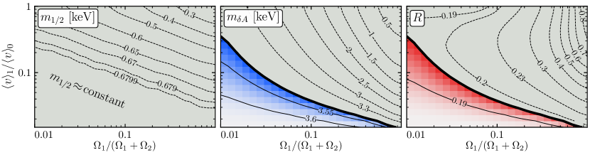
Figure 11: Contours in the $(\Omega_{1}/(\Omega_{1}+\Omega_{2}),\left\langle v\right\rangle_{1}/\left\langle v\right\rangle_{0})$-plane of ${m_{1/2}}$ (left panel) and $m_{\delta A}$ (center panel), as well as the comparator $R$ (right panel), for the general phase-space distribution in Eq. (23) with $N_{G}=3$. The results shown correspond to the choices $\left\langle v\right\rangle_{0}=10^{-6}$, $\sigma_{0}=\sigma_{1}=\sigma_{2}=0.63$, $\Omega_{0}/\Omega=4.8\times 10^{-2}$, and $\left\langle\log v\right\rangle_{12}=-18.21$. The thick black curves in the center and right panels indicate the Lyman-$\alpha$ constraints obtained by employing the bound ${m_{\rm WDM}}\gtrsim 3.5\,{\rm keV}$ in implementing the $\delta A$ recast. The gray regions above and to the right of these constraint contours are excluded.

V.2 The Effects of Additional Modes

Our analysis of the bi-modal distributions in the previous section constitutes a necessary first step in establishing Lyman-$\alpha$ constraints on Class-II velocity distributions. However, the results of this analysis prompt several additional questions. Perhaps the most important such question concerns the manner in which the Lyman-$\alpha$ constraints that we have derived for the $g(p)$ distribution in Eq. (23) with $N_{G}=2$ generalize to the case in which $N_{G}>2$.

Given that a systematic survey of the full parameter space of possible $g(p)$ distributions is impractical for $N_{G}>2$, we shall investigate the answer to this question according to the procedure outlined at the beginning of this section. We begin by identifying an illustrative benchmark point within the $N_{G}=2$ parameter space that we examined above. We then examine the subspace of the full $N_{G}=3$ parameter space associated with bifurcations of the lowest-velocity peak in the $g(p)$ distribution for this benchmark for which the center of velocity $\left\langle\log v\right\rangle_{12}$ is the same as it was for that original peak. We adopt as our parameter-space benchmark a point which lies directly on one of the exclusion contours in Fig. 8. In particular, we choose the point $(\Omega_{0}/\Omega,\langle v\rangle_{1}/\langle v\rangle_{0})=(4.8\times 10^{-2},0.015)$ indicated by the green star appearing in the bottom panels of Fig. 8. We take the two free parameters which describe the possible bifurcations of the low-velocity peak in this distribution consistent with our condition on $\left\langle\log v\right\rangle_{12}$ to be $\left\langle v\right\rangle_{1}/\left\langle v\right\rangle_{0}$ and $\Omega_{1}/(\Omega_{1}+\Omega_{2})$.

In Fig. 11, we show contours of ${m_{1/2}}$ (left panel), $m_{\delta A}$ (center panel), and $R$ (right panel) in the $(\Omega_{1}/(\Omega_{1}+\Omega_{2}),\left\langle v\right\rangle_{1}/\left\langle v\right\rangle_{0})$-plane for the values of $\Omega_{0}/\Omega$, $\left\langle v\right\rangle_{0}$, $\sigma_{0}$, $\sigma_{1}$, $\sigma_{2}$, and $\left\langle\log v\right\rangle_{12}$ specified above. The bottom right corner of each panel corresponds to the location of our benchmark point within this space. The thick black curves in the center and right panels represent the Lyman-$\alpha$ exclusion contours obtained by employing the bound ${m_{\rm WDM}}\gtrsim 3.5\,{\rm keV}$ in implementing the $\delta A$ recast. The gray regions above and to the right of these contours are excluded. We observe that each of these contours terminates on and includes our benchmark. Indeed, this is to be expected, given that this benchmark corresponds to a point which lies along the exclusion contour in Fig. 8 obtained from the same recast. By contrast, we find that the entirety of the parameter space shown in Fig. 11 is excluded according to the half-mode recast. This is not unexpected either, given that our benchmark lies well within the region of the $(\Omega_{0}/\Omega,\left\langle v\right\rangle_{1}/\left\langle v\right\rangle_{0})$-plane in Fig. 8 which is excluded according to this same recast.

Generally speaking, we observe from Fig. 11 that increasing either the relative abundance $\Omega_{1}/(\Omega_{1}+\Omega_{2})$ or the average velocity $\langle v\rangle_{1}$ of the intermediate-velocity peak decreases both ${m_{1/2}}$ and $m_{\delta A}$ and thus increases the tension with Lyman-$\alpha$ data. These results accord well with our qualitative expectations, given that we are holding $\Omega_{1}+\Omega_{2}$ and $\left\langle\log v\right\rangle_{12}$ fixed as we vary these other quantities. Indeed, increasing either $\Omega_{1}/(\Omega_{1}+\Omega_{2})$ or $\langle v\rangle_{1}$ increases the differential number density of dark-matter particles at higher $v$ and enhances the suppression of power at lower $k$ due to free-streaming effects. Moreover, the shapes of the contours in the left two panels of Fig. 11 provide interesting additional information about how the results of the two recasts depend on the properties of the two lower-velocity peaks. In particular, they indicate that the values of both ${m_{1/2}}$ and $m_{\delta A}$ are more sensitive to changes in $\left\langle v\right\rangle_{1}/\left\langle v\right\rangle_{0}$ than they are to $\Omega_{1}/(\Omega_{1}+\Omega_{2})$, at least in the regime in which latter quantity is sizable. Indeed, it is only for $\Omega_{1}/(\Omega_{1}+\Omega_{2})\lesssim 0.05$ that the slope of the exclusion contour associated with the $\delta A$ recast steepens.

Most importantly, however, we see from Fig. 11 that our comparator $R$ can again differ significantly from unity, and moreover does so precisely within the region of parameter space which is considered viable according to our recasts. This reinforces the cautionary note — already observed from Fig. 8 — that our recasts can yield Lyman-$\alpha$ constraints which differ significantly from each other for complex, multi-modal dark-matter phase-space distributions.

VI Comparison with Parametric-Function Techniques

Our primary focus in this paper has been to illustrate the pitfalls which can arise when the half-mode and $\delta A$ recasts are employed in order to estimate Lyman-$\alpha$ constraints on dark-matter scenarios with Class-II velocity distributions. Of course, there exists an alternative method for estimating Lyman-$\alpha$ constraints on non-cold dark-matter scenarios [20]. This method involves positing a simple, parametric model for $T^{2}(k)$ and performing numerical simulations in order to evaluate the corresponding flux power spectra at a representative sample of points within the parameter space of that model. These spectra can then be compared to observed flux power spectra in order to determine which regions of that parameter space are consistent with Lyman-$\alpha$ data and which are excluded. Once a survey of this sort has been performed, constraints on a given dark-matter scenario can be estimated by fitting the transfer function obtained for that scenario to the parametric model. If the best-fit values for the parameters of that model lie within an excluded region, the dark-matter scenario is excluded.

Such a survey was performed in Ref. [26] using the parametric function [20]

$$T^{2}(k)~{}=~{}[1+(\alpha k)^{\beta}]^{2\gamma}~{},$$ (25)

where $\alpha\geq 0$, $\beta>0$, and $\gamma>0$ are the free parameters which characterize the model. The authors of Ref. [26] employed hydrodynamic simulations in order to place Lyman-$\alpha$ constraints on the three-dimensional parameter space of this model based on a scan over a large number of combinations of $\alpha$, $\beta$, and $\gamma$.

While the parametric function in Eq. (25) is capable of modeling a broad range of transfer functions quite accurately, in general it is not capable of modeling accurately the kinds of transfer functions that arise from Class II velocity distributions. Indeed, as was shown in Eqs. (3.19) – (3.21) of Ref. [6], the matter power spectra described by this parametric function are characteristic of strictly unimodal $g(p)$ distributions.

The implications that this property of the parametric function in Eq. (25) has for establishing Lyman-$\alpha$ constraints on dark-matter models with Class II velocity distributions are perhaps best conveyed by means of concrete examples. In the top panel of Fig. 12, we show the transfer functions (solid magenta, green, and blue curves) obtained for the three parameter-space points indicated by the stars of the corresponding colors in the bottom panels of Fig. 8. The the point indicated by the blue star corresponds to the parameter assignments $(\Omega_{0}/\Omega,\left\langle v\right\rangle_{1}/\left\langle v\right\rangle_{0})=(0.032,10^{-3})$. This point, which lies within the allowed region in Fig. 8 associated with the $\delta A$ recast, is excluded according to the $m_{1/2}$ recast. However, the corresponding transfer function represents a far more dramatic departure from the transfer functions characteristic of Class-I velocity distributions than do the transfer functions obtained for the other two parameter-space points. In the bottom panel, we show the $g(p)$ distributions for these three parameter-space points. We note that the ranges of $k$ associated with the individual peaks in each of these $g(p)$ distributions align with the ranges of $k$ within which the corresponding $T^{2}(k)$ curve exhibits a significant decrease in its slope. The relationship between features in $g(p)$ and $T^{2}(k)$ suggested by this juxtaposition is articulated more concretely in Ref. [6].

In the top panel of Fig. 12, we also show the transfer function (dashed curve of the corresponding color) which represents the best fit to the true $T^{2}(k)$ curve for each of three parameter-space points using the parametrization in Eq. (25). The values of $\alpha$, $\beta$, and $\gamma$ for each of these best-fit curves are provided in the legend. The yellow and gray curves represent the transfer functions of the form given in Eq. (25) for the combinations of $\alpha$, $\beta$, and $\gamma$ included in the parameter-space survey performed in Ref. [26]. The yellow curves represent the transfer functions which were found to be consistent with Lyman-$\alpha$ constraints, while the gray curves represent the transfer functions which were found to be excluded.

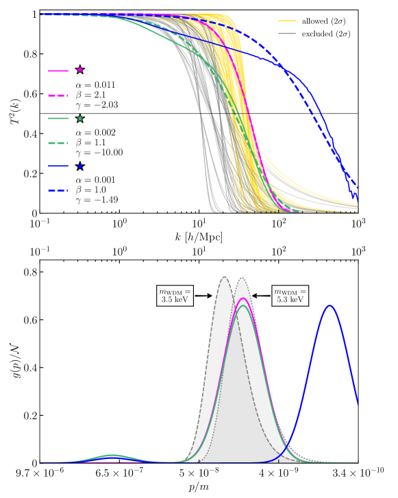
Figure 12: Top panel: The solid magenta and green curves represent the transfer functions obtained for the parameter-space points indicated by the stars of the corresponding colors in Fig. 8, while the solid blue curve represents the transfer function obtained for the parameter-space point with the same $\left\langle v\right\rangle_{0}$, $\sigma_{0}$, and $\sigma_{1}$ values as these other two points, but with $\Omega_{0}/\Omega=0.032$ and $\left\langle v\right\rangle_{1}/\left\langle v\right\rangle_{0}=10^{-3}$. The dashed curves of the corresponding colors represent the best-fit functions of the form given in Eq. (25) to these three curves. The best-fit values of the parameters $\alpha$, $\beta$, and $\gamma$ in each case are provided in the legend. The yellow and gray curves represent the transfer functions of the form given in Eq. (25) for the combinations of $\alpha$, $\beta$, and $\gamma$ included in the survey performed in Ref. [26]. The yellow curves represent the transfer functions which were found to be consistent with Lyman-$\alpha$constraints, while the gray curves represent the transfer functions which were found to be excluded. Bottom panel: The $g(p)$ distributions which give rise to the $T^{2}(k)$ curves of the corresponding colors in the top panel. The value of $k$ above which the dark-matter particles in $g(p)$ with velocity $p/m$ can suppress power due to free-streaming effects is indicated by the tick marks on the top axis. These $g(p)$ distributions are displayed such that these tick marks are uniformly spaced on a logarithmic scale and such that $k$ increases from left to right. The corresponding $p/m$ values indicated on the bottom axis are therefore spaced non-uniformly and increase from right to left. The $g(p)$ distributions for WDM models with ${m_{\rm WDM}}=3.5$ keV and ${m_{\rm WDM}}=5.3$ keV, which are indicated by the dashed and dotted gray curves, respectively, are also included for reference.

For the magenta $g(p)$ distribution — a distribution for which the relative abundance $\Omega_{0}/\Omega\approx 7.0\times 10^{-4}$ of the higher-velocity peak is quite small — we observe that the parametrization in Eq. (25) provides an excellent fit to the corresponding transfer function. Since this transfer function lies well within the region spanned by the yellow curves, it is clear that this distribution would not be excluded by Lyman-$\alpha$ constraints according to the simulations performed in Ref. [26]. According to the the half-mode recast, this $g(p)$ distribution would be marginal, while according to the $\delta A$ recasts, it would be allowed, as shown in Fig. 8. In this case, then, the results obtained using the parametric function in Eq. (25) are more consistent with the results of the $\delta A$ recast.

By contrast, for the green $g(p)$ distribution, the best fit to the corresponding transfer function using the functional parametrization in Eq. (25) differs more significantly from the true $T^{2}(k)$ curve. Indeed, for wavenumbers within the range $1h/{\rm Mpc}\lesssim k\lesssim 20h/{\rm Mpc}$, the relative error can be as high as $5\%$. Nevertheless, it is still reasonable to assume that this $g(p)$ distribution is excluded. Indeed, the $T^{2}(k)$ curve obtained from the fit reflects a significant suppression of power within the relevant range of $k$ and lies well within the region spanned by the gray curves, while the true $T^{2}(k)$ curve is even further suppressed. This $g(p)$ distribution would likewise be excluded by the half-mode recast, while according to the $\delta A$ recast it would be marginal. In this case, then, the results obtained using the parametric function in Eq. (25) are more consistent with the results of the half-mode recast.

Finally, for the blue $g(p)$ distribution, the best fit to the corresponding transfer function using the functional parametrization in Eq. 25 overestimates the true value of $T^{2}(k)$ by as much $12\%$ for wavenumbers within the range $1h/{\rm Mpc}\lesssim k\lesssim 100h/{\rm Mpc}$. Based solely on the $T^{2}(k)$ curve obtained from the fit, one would conclude that this $g(p)$ distribution is allowed, given that it lies well within the region spanned by the yellow curves. However, the true $T^{2}(k)$ curve lies significantly below this best-fit curve throughout most of the relevant range of $k$. Thus, we cannot conclusively determine whether the corresponding $g(p)$ distribution is allowed or excluded by comparing with the simulation results provided in Ref. [26]. Thus, for Class II velocity distributions of this sort, Lyman-$\alpha$ constraints obtained from this parametric-function technique are not necessarily any more reliable than those obtained from the half-mode or $\delta A$ recasts.

Taken together, the results displayed in Fig. 12 indicate that while the parametric function in Eq. (25) may capture the gross features of the transfer functions associated with certain Class-II dark-matter velocity distributions (particularly those that resemble Class-I distributions), they do not generically provide an accurate fit to these $T^{2}(k)$. Indeed, the more significantly $g(p)$ departs from the Class-I velocity distributions that we examined in Sect. IV, the less accurate the fit to the corresponding $T^{2}(k)$ becomes. Thus, for velocity distributions of this sort, the Lyman-$\alpha$ constraints obtained from this parametric function are not necessarily any more reliable than those obtained from the half-mode or $\delta A$ recasts.

That said, the results displayed in Fig. 12 also highlight the importance of performing hydrodynamic simulations on dark-matter models beyond the baseline WDM model in deriving Lyman-$\alpha$ constraints. The parametric-function technique developed in Ref. [26] provides a benchmark for establishing such constraints on dark-matter models with more general velocity distributions. Indeed, while the parametric function in Eq. (25) is not capable of modeling accurately the kinds of transfer functions that arise from Class II velocity distributions, an analysis similar to the one performed in Ref. [26], but with a more adaptable parametric function could in principle extend the applicability of this technique to velocity distributions within this class.

VII Conclusions

In this paper, we have conducted a preliminary investigation into the constraints imposed by Lyman-$\alpha$-forest data on general dark-matter velocity distributions. In particular, we have investigated the bounds obtained from two common methods of recasting the Lyman-$\alpha$ constraints onto a baseline WDM model — methods which are frequently employed in order to estimate these constraints in situations in which it would be impractical to perform the hydrodynamic simulations that would otherwise be necessary. In order to conduct this study, we also introduced two new quantities — our critical mass parameters ${m_{1/2}}$ and $m_{\delta A}$ — which enabled us to compare the results of these two recasts in a systematic, quantitative way.

After evaluating the Lyman-$\alpha$ constraints on a baseline WDM velocity distribution, we applied our methods in order to study departures from this baseline distribution. We began by examining how Lyman-$\alpha$ constraints are affected by comparatively mild departures, such as replacing this distribution with a Gaussian distribution and varying the width of the distribution. Even for such simple, Class-I velocity distributions, we demonstrated that disagreements arose between the results obtained from the half-mode and $\delta A$ recasts. We then extended this study to encompass dark-matter velocity distributions which represent a even more dramatic departures from our baseline distribution, including multi-modal distributions consisting of superpositions of Gaussian peaks. The impact of free-streaming on $T^{2}(k)$ in these cases is more subtle, given that different parts of these velocity distributions have different thresholds in $k$ above which they contribute to the suppression of power. Even for the simplest possible such distributions, which comprise only two Gaussian peaks, we have demonstrated that dramatic disagreements between ${m_{1/2}}$ and $m_{\delta A}$ — and therefore between the Lyman-$\alpha$ constraints obtained for the two recasts — can arise. We also examined how these results are modified by the incorporation of additional peaks into these dark-matter velocity distributions.

While the results in Sect. V serve to highlight how disagreements between the half-mode and $\delta A$ recasts arise for Class-II velocity distributions, we can make no statement as to which of these recasting methods provides a more accurate representation of the Lyman-$\alpha$ constraint for a given dark-matter velocity distribution without performing the necessary hydrodynamic simulations. Nevertheless, our findings provide important insights into how highly non-trivial velocity distributions of this sort are constrained by Lyman-$\alpha$ data. First, our results provide qualitative information about how the Lyman-$\alpha$ constraints on particular kinds of dark-matter velocity distributions are likely to be affected when certain features of those distributions are modified. Second, however, our results provide general indications as to when each of these recasts is likely to be reliable and when it is likely to be unreliable across the landscape of possible Class-II velocity distributions. In this way, our results serve as a cautionary tale concerning the implementation of these recasts and highlight the kinds of distributions for which the need for dedicated numerical analysis is the most pressing.

Several additional comments are in order. First, while we have taken a step toward exploring the Lyman-$\alpha$ constraints on the landscape of possible Class-II dark-matter velocity distributions, this landscape is vast and there are a number of areas that merit further exploration. Indeed, while a wide variety of such distributions can be decomposed according to Eq. (23) with reasonably fidelity, such a Gaussian decomposition cannot capture every feature of a generic function perfectly. It does not, for example, permit us to study the extent to which the exclusion contours are sensitive to the detailed shapes of the individual peaks.

Second, along similar lines, there are other aspects of Class-I velocity distributions which merit further exploration as well. In particular, we would like to know how general modifications of the shape of the peak can affect the results of the half-mode and $\delta A$ recasts. This shape may be quantitatively characterized by its different moments — the average momentum, standard deviation, skewness, kurtosis, etc.  We have examined the effect of varying the first two of these moments in Sect. IV, but there are many reasons to expect that the higher moments also have a significant impact on the results of these recasts, particularly for a distribution with a sizable width. For example, a positively skewed distribution contains a higher proportion of low-velocity particles than a symmetric distribution does. As a result, the suppression of structure due to free-streaming may become particularly pronounced only at smaller scales (corresponding to larger $k$). By contrast, a negatively skewed distribution contains a higher proportion of high-velocity particles than does a symmetric distribution does. As a result, the suppression of structure can become significant at even larger distance scales (corresponding to smaller $k$). Such effects on $T^{2}(k)$ are likely to have have an impact on the results of our recasts. Indeed, as discussed in Ref. [6], the skewness of the dark-matter velocity distribution is directly connected to fundamental properties of the dark-matter production mechanism.

Finally, our study in this paper was performed under the assumption that the shape of the dark-matter phase-space distribution is essentially fixed well before the time of matter-radiation equality. For this reason, our analysis may not be applicable to scenarios in which $g(p,t)$ is still dynamically evolving at subsequent times, when matter perturbations are growing at a significant rate. Such complications may arise for models in which the dark matter has non-negligible self-interactions [23]. Such complications may also arise in multi-component dark-matter models wherein the heavier dark-matter species are unstable but long-lived and decay primarily to final states comprising lighter dark-matter species. Indeed, this is what occurs within the context of the Dynamical Dark Matter framework [41, 42, 43]. The resulting gradual conversion of mass energy to kinetic energy within the dark sector can then “heat up” the dark matter at late times, resulting in a non-trivial modification of the dark-matter velocity distribution. Indeed, for certain scenarios of this sort, numerical studies have been performed in order to investigate the impact of this effect on the Lyman-$\alpha$ forest [44] and on other aspects of small-scale structure [45, 46].