A new locally linear embedding scheme in light of Hessian eigenmap

Abstract

We provide a new interpretation of Hessian locally linear embedding (HLLE), revealing that it is essentially a variant way to implement the same idea of locally linear embedding (LLE). Based on the new interpretation, a substantial simplification can be made, in which the idea of “Hessian” is replaced by rather arbitrary weights. Moreover, we show by numerical examples that HLLE may produce projection-like results when the dimension of the target space is larger than that of the data manifold, and hence one further modification concerning the manifold dimension is suggested. Combining all the observations, we finally achieve a new LLE-type method, which is called tangential LLE (TLLE). It is simpler and more robust than HLLE.

1 Introduction

Let $\mathcal{X}=\{x_{i}\}_{i=1}^{N}$ be a collection of data points in some $\mathbb{R}^{D}$. The goal of nonlinear dimensionality reduction (or manifold learning) is to find for $\mathcal{X}$ a representation $\mathcal{Y}=\{y_{i}\}_{i=1}^{N}$ in some lower dimensional $\mathbb{R}^{d}$, under the assumption that $\mathcal{X}$ lies on some unknown submanifold $\mathcal{M}$ in $\mathbb{R}^{D}$.

Among the several existing manifold learning methods, Hessian eigenmap [2], also called Hessian locally linear embedding (HLLE), is one that exhibits prominent performance on the popular synthetic data “Swiss roll with a hole”. It can be regarded as a generalization of Laplacian eigenmap [1] in some respect or LLE [4] in another. However, its procedure concerning the construction and minimization of “Hessian” is much more sophisticated.

In this paper, we will provide a new interpretation of the mechanism behind HLLE, revealing that what it really does follows the same idea as LLE: Asking $\mathcal{Y}$ to satisfy the local linear relations for $\mathcal{X}$ as best as possible. The main differences lie in their ways of describing the local linear relations. Roughly speaking, HLLE only fits local linear relations of the $d$-dimensional principal components, and at the same time exploits multiple weights to do this job. Based on this understanding, we are able to make a substantial simplification, in which the idea of “Hessian” is totally abandoned. Indeed, we will show that the Hessian estimators in HLLE, which are specially designed matrices, can be replaced by rather arbitrary weight matrices.

Moreover, we observe that when the dimension of the target space $d$ is greater than that of the data manifold $\mathcal{M}$, a naive application of HLLE may result in a type of unwanted result, which looks like some direct projection of $\mathcal{X}$ onto $\mathbb{R}^{d}$. Such “projection patterns” are also observed for LLE (see Section 3, or [3] for detailed discussion). For HLLE, they do not appear in the embedding of the Swiss roll in the plane, for which $d=\dim\mathcal{M}=2$. However, in general a manifold may not be able to be well embedded in a Euclidean space of the same dimension, and setting $d$ to be larger than $\dim\mathcal{M}$ might be more suitable. In such a situation, some modification has to be made to avoid the projection patterns. Combining the mentioned simplification and this modification, we finally achieve a new LLE-type method, which will be named tangential LLE (TLLE).

2 New interpretation of HLLE

As in the introduction, in the following let $\mathcal{X}=\{x_{i}\}_{i=1}^{N}$ be a dataset in $\mathbb{R}^{D}$, which is supposed to lie on some unknown submanifold $\mathcal{M}$ (sometimes referred to as the data manifold), and our goal is to find for $\mathcal{X}$ a representation $\mathcal{Y}=\{y_{i}\}_{i=1}^{N}$ in some lower dimensional $\mathbb{R}^{d}$.

We first review the procedure of HLLE, given as (H1) $\sim$ (H4) below. The idea will be (partly) discussed right after.

1. For each $i=1,\ldots,N$ let $\mathcal{U}_{i}=\{x_{i_{1}},\ldots,x_{i_{k}}\}\subset\mathcal{X}\setminus\{x_{i}\}$ be a $k$-nearest neighborhood of $x_{i}$, where

   $$k\geq 1+d+\frac{d(d+1)}{2}.$$

   For simplicity we consider $k$ to be a fixed number for all $i$.

2. Let

   $$M^{(i)}=\begin{bmatrix}x_{i_{1}}-\overline{x}_{i}&\cdots&x_{i_{k}}-\overline{x}_{i}\end{bmatrix}\in\mathbb{R}^{D\times k},$$

   where $\overline{x}_{i}=\frac{1}{k}\sum_{j=1}^{k}x_{i_{j}}$. Find the singular value decomposition

   $$M^{(i)}=U^{(i)}\Sigma^{(i)}V^{(i)T},$$

   where $U^{(i)}$ is a $D\times D$ orthogonal matrix whose columns will be denoted by $u_{1}^{(i)},\ldots,u_{D}^{(i)}$, $\Sigma^{(i)}$ is a $D\times k$ diagonal matrix with diagonal entries $\sigma_{1}^{(i)}\geq\cdots\geq\sigma_{\min(D,k)}^{(i)}\geq 0$, and $V^{(i)}$ is a $k\times k$ orthogonal matrix with columns $v_{1}^{(i)},\ldots,v_{k}^{(i)}$.

3. Let $V_{d}^{(i)}=[v_{1}^{(i)}\ \cdots\ v_{d}^{(i)}]\in\mathbb{R}^{k\times d}$ be the matrix consisting of the first $d$ columns of $V^{(i)}$, and let $V_{d}^{(i)}\boxtimes V_{d}^{(i)}\in\mathbb{R}^{k\times d(d+1)/2}$ be the matrix whose columns are all the vectors $v_{s}^{(i)}v_{t}^{(i)}$, $1\leq s\leq t\leq d$, listed in any prescribed order. Here $ab$ for two (column) vectors $a=(a_{1},\ldots,a_{k})$ and $b=(b_{1},\ldots,b_{k})$ denotes their componentwise product $(a_{1}b_{1},\ldots,a_{k}b_{k})$. Let $\boldsymbol{1}_{k}\in\mathbb{R}^{k}$ be the vector whose components are all equal to $1$, and let

   $$G^{(i)}=\begin{bmatrix}\boldsymbol{1}_{k}&V_{d}^{(i)}&V_{d}^{(i)}\boxtimes V_{d}^{(i)}\end{bmatrix},$$

   which is a matrix of size $k\times(1+d+\frac{d(d+1)}{2})$. Apply the Gram-Schmidt process to the columns of $G^{(i)}$ to obtain a new matrix with orthonormal columns, and let $H^{(i)}$ be the submatrix of this new matrix consisting of the last $d(d+1)/2$ columns (the position of $V_{d}^{(i)}\boxtimes V_{d}^{(i)}$ in $G^{(i)}$).

4. Set $\mathcal{Y}$ to be a solution to the minimization problem

   $$\underset{\{y_{i}\}_{i=1}^{N}\subset\mathbb{R}^{d}}{\mbox{argmin}}\sum_{i=1}^{N}\|Y_{i}H^{(i)}\|^{2}\quad\mbox{s.t.}\quad YY^{T}=I,$$

   where $Y=\left[y_{1}\ \cdots\ y_{N}\right]\in\mathbb{R}^{d\times N}$ and $Y_{i}=\left[y_{i_{1}}\ \cdots\ y_{i_{k}}\right]\in\mathbb{R}^{d\times k}$. Here $\|A\|$ for a matrix $A=(a_{ij})$ denotes the Frobenius norm $\sqrt{\sum_{i,j}a_{ij}^{2}}$.

Before giving our new interpretation of HLLE, we make some preliminary remarks and comments about its original idea. First, what (H2) does is to perform the principal component analysis for $\mathcal{U}_{i}$. The $d$-dimensional principal component of $x_{i_{j}}$ ($j=1,\ldots,k$), denoted by $\widetilde{x}_{i_{j}}$ later on, is the orthogonal projection of $x_{i_{j}}$ on the $d$-dimensional hyperplane

$$\mathcal{T}_{i}:=\overline{x}_{i}+\mbox{span}(u_{1}^{(i)},\ldots,u_{d}^{(i)}).$$ (1)

Accordingly, we will use $\widetilde{\mathcal{U}}_{i}$ to denote the set $\{\widetilde{x}_{i_{1}},\ldots,\widetilde{x}_{i_{k}}\}$. By setting the canonical coordinate system on $\mathcal{T}_{i}$ in which $\overline{x}_{i}$ is the origin and $u_{1}^{(i)},\ldots,u_{d}^{(i)}$ are the directions of the coordinate axes, we can regard $\widetilde{x}_{i_{j}}$, $j=1,\ldots,k$, as vectors in $\mathbb{R}^{d}$, whose coordinates are given by the first $d$ rows of $\Sigma^{(i)}V^{(i)T}$. That is,

$$\begin{bmatrix}\widetilde{x}_{i_{1}}&\cdots&\widetilde{x}_{i_{k}}\end{bmatrix}=\begin{bmatrix}\sigma_{1}^{(i)}\\ &\ddots\\ &&\sigma_{d}^{(i)}\end{bmatrix}\begin{bmatrix}v_{1}^{(i)T}\\ \vdots\\ v_{d}^{(i)T}\end{bmatrix}=\begin{bmatrix}\sigma_{1}^{(i)}v_{1}^{(i)T}\\ \vdots\\ \sigma_{d}^{(i)}v_{d}^{(i)T}\end{bmatrix}.$$ (2)

The $j$-th row $\sigma_{j}^{(i)}v_{j}^{(i)T}$ hence represents the $j$-th coordinate function on $\widetilde{\mathcal{U}}_{i}$.

The geometrical motivation of Step (H2) is that, if the dimension $d$ of the target space is the same as that of the data manifold $\mathcal{M}$, then $\mathcal{T}_{i}$ is an approximation of the tangent space at $x_{i}$. Therefore, $\widetilde{\mathcal{U}}_{i}$ represents the tangential component of $\mathcal{U}_{i}$. This motivation however is totally ignored in the implementation, and the algorithm of HLLE can run without checking whether $d=\dim\mathcal{M}$. Thus, there comes a question: Is this equality in dimension important, or can it be safely ignored? Possibly a bit unexpectedly, it really matters – for the original HLLE. Of course, if $d<\dim\mathcal{M}$, it is no surprise that there will be a heavy loss in fidelity. What interesting is that choosing $d>\dim\mathcal{M}$ would also cause HLLE to produce unwanted results. We will discuss about this issue and give a simple solution to it in Section 4. For now let us assume $d=\dim\mathcal{M}$.

Now move on to (H3). Our definition of $G^{(i)}$ in (H3) follows the original paper [2], while some researchers (for example [5, 6]) set $G^{(i)}$ to be $\left[\boldsymbol{1}_{k}\ F^{(i)}\ F^{(i)}\boxtimes F^{(i)}\right]$, where $F^{(i)}:=[\sigma^{(i)}_{1}v^{(i)}_{1}\,\cdots\,\sigma^{(i)}_{d}v^{(i)}_{d}]\in\mathbb{R}^{k\times d}$. In normal situations we have $\mbox{rank}(M^{(i)})\geq d$, and hence its first $d$ singular values $\sigma_{1}^{(i)},\ldots,\sigma_{d}^{(i)}$ are nonzero. We will assume this throughout the paper. Thus the only difference between the two definitions of $G^{(i)}$ is that each corresponding column may differ by a nonzero factor. As a consequence, they give rise to the same $H^{(i)}$ after performing the Gram-Schmidt process.

In [2], $H^{(i)}$ is claimed to be a Hessian estimator on $\mathcal{U}_{i}$, and the motivation of asking $\mathcal{Y}$ to solve the minimization problem in (H4) is based on the fact that if $\mathcal{Y}$ can be obtained from $\mathcal{X}$ through some isometric mapping from $\mathcal{M}$ to $\mathbb{R}^{d}$ (the most ideal situation), then the global intrinsic coordinate functions on $\mathcal{M}$ (which are represented by the rows of $Y$) should have zero second order derivatives everywhere. These claims themselves are worthy of more explanations and discussions. However, we shall not pursue this direction here. Instead, we will provide a much simpler interpretation of the mechanism behind (H3) and (H4).

First let us go back to (H2). Since the columns of $M^{(i)}$ have mean zero,

$$0=M^{(i)}\boldsymbol{1}_{k}=U^{(i)}\Sigma^{(i)}V^{(i)T}\boldsymbol{1}_{k}.$$

Then, since $U^{(i)}$ is invertible, and since the first $d$ singular values $\sigma_{1}^{(i)},\ldots,\sigma_{d}^{(i)}$ are assumed to be nonzero, $V_{d}^{(i)T}\boldsymbol{1}_{k}=0$. Thus, the first $1+d$ vectors $\boldsymbol{1}_{k},v_{1}^{(i)},\ldots,v_{d}^{(i)}$ in $G^{(i)}$ are already orthogonal to each other. As a consequence, the Gram-Schmidt process in (H3) does not change them except for normalizing $\boldsymbol{1}_{k}$ to $\frac{1}{\sqrt{k}}\boldsymbol{1}_{k}$ (which is also redundant as we only need the result of the last $d(d+1)/2$ columns).

Now let us use $h=(h_{1},\ldots,h_{k})^{T}$ to denote any one of the $d(d+1)/2$ columns of $H^{(i)}$. By construction $h$ is a unit vector perpendicular to $\boldsymbol{1}_{k},v_{1}^{(i)},\ldots,v_{d}^{(i)}$. In particular, it is perpendicular to $\sigma_{1}^{(i)}v_{1}^{(i)},\ldots,\sigma_{d}^{(i)}v_{d}^{(i)}$. From (2), this last statement can be written as

$$\begin{bmatrix}\widetilde{x}_{i_{1}}&\cdots&\widetilde{x}_{i_{k}}\end{bmatrix}\begin{bmatrix}h_{1}\\ \vdots\\ h_{k}\end{bmatrix}=0,$$

which is nothing but a linear relation on $\widetilde{\mathcal{U}}_{i}$:

$$h_{1}\widetilde{x}_{i_{1}}+\cdots+h_{k}\widetilde{x}_{i_{k}}=0.$$ (h1)

Thus, the use of $H^{(i)}$ is that each of its columns describes a linear relation on $\widetilde{\mathcal{U}}_{i}$. With all of the columns, it then provides a total of $d(d+1)/2$ linear relations. All together they can be expressed as

$$\begin{bmatrix}\widetilde{x}_{i_{1}}&\cdots&\widetilde{x}_{i_{k}}\end{bmatrix}H^{(i)}=0.$$ (3)

On the other hand, the facts that $h$ is perpendicular to $\boldsymbol{1}_{k}$ and that $h$ is a unit vector amount to two constraints on the coefficients:

$$\sum_{j=1}^{k}h_{j}=0,$$ (h2)

$$\sum_{j=1}^{k}h_{j}^{2}=1.$$ (h3)

From the above point of view, the purpose of Step (H4) is also clear: It simply asks $\mathcal{Y}$ to satisfy the same local linear relations as (3) as best as possible. Thus what HLLE does, in this new interpretation, is really in the same vein as LLE, only that their ways of describing local linear relations are different (see Section 3 for some comparisons).

Now, for convenience let us call any vector $(h_{1},\ldots,h_{k})$ which satisfies (h1) $\sim$ (h3) an $h$-weight. An essential simplification which can be made from the above new understanding of HLLE is that we may choose $H^{(i)}$ arbitrarily as long as its columns are constituted by $h$-weights! It needs not be constructed from the specially designed $V_{d}^{(i)}\boxtimes V_{d}^{(i)}$ in (H3), and also its number of columns needs not be $d(d+1)/2$. The number of columns in $H^{(i)}$, call it $m$, just indicates how many $h$-weights we would like to use to characterize the linear relation on $\widetilde{\mathcal{U}}_{i}$. It is a number we can decide at will, subject only to the slight restriction $k\geq 1+d+m$ (replacing the stronger requirement $k\geq 1+d+d(d+1)/2$ given in (H1)), since the vectors $\boldsymbol{1}_{k},v_{1}^{(i)},\ldots,v_{d}^{(i)}$ and the columns of $H^{(i)}$ have to be linearly independent. In other words,

we have to choose $k\geq d+2$ in (H1), and then $m$ can be any number between $1,2,\ldots,k-d-1$.

To implement the new idea, it is still convenient to make use of the Gram-Schmidt process to generate $h$-weights. The only modification from the original HLLE is that we can replace $V_{d}^{(i)}\boxtimes V_{d}^{(i)}$ by other matrices, as long as the columns of $G^{(i)}$ form a linearly independent set. For this purpose, it is reasonable to resort to a random construction. Precisely, we replace (H3) by the following:

• Select $m$ random vectors $r_{1},\ldots,r_{m}$ in $\mathbb{R}^{k}$, and perform the Gram-Schmidt process to the columns of

  $$G^{(i)}:=\begin{bmatrix}\boldsymbol{1}_{k}&v_{1}^{(i)}&\cdots&v_{d}^{(i)}&r_{1}&\cdots&r_{m}\end{bmatrix}$$

  to obtain a new matrix with orthonormal columns. Then set $H^{(i)}\in\mathbb{R}^{k\times m}$ to be the submatrix consisting of the last $m$ columns.

The new method will be called tangential LLE (TLLE). We stress again that here we only consider cases with $d=\dim\mathcal{M}$. In Section 4 we will add one further modification in order to cover also cases with $d>\dim\mathcal{M}$, and a written down algorithm for that final version will be given there.

We also stress that $k\geq d+2$ is a minimum restriction in principle. From experiments, larger $k$ is usually needed. On the other hand, much fewer $h$-weights than $k-d-1$ may work pretty well. Nevertheless, it looks like using multiple weights, i.e. $m\geq 2$, is crucial to ensure good results. Figure 1 shows some numerical simulations on the Swiss roll with a hole ($d=2$).

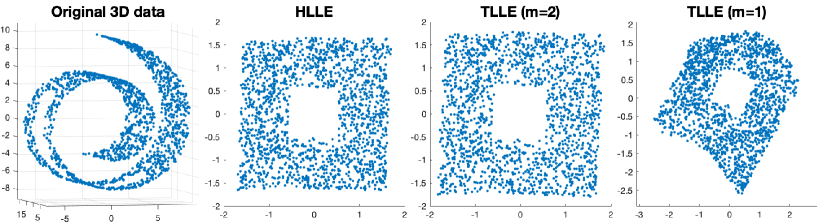
Figure 1: Numerical results for Swiss roll with a hole by HLLE ($k=8$) and TLLE ($k=8$; $m=2$ and $m=1$).

Each of the simulations adopts $k=8$. For TLLE, largest possible $m$ is $8-2-1=5$, while $m=2$ already gives equally good result as HLLE (which can be regarded as using $m=3$). In fact, the outcomes of HLLE and TLLE ($m=2$) look identical! (The two pictures differ only in size, which is merely a consequence of scaling.) This is not a coincidence but is usually the case from our repeated experiments. Though astonishing at first sight, this phenomenon simply reflects the fact that both results are almost perfect: They both unfold the 3D data faithfully without messing up any part.

3 Comparison of LLE and TLLE

In this section we also consider $d=\dim\mathcal{M}$. We have mentioned that TLLE (in particular HLLE) implements essentially the same idea as LLE: Asking $\mathcal{Y}$ to fit the local linear relations of $\mathcal{X}$ as best as possible. The main differences lie in their ways of describing local linear relations. In this section we take a close look at some of the differences. Readers who would like to know the practical usage of TLLE quickly may read only point (A) below to have a basic understanding of “projection pattern”, and then go straight to the next section.

For convenience we give a review of the procedure of LLE first. It goes as follows:

1. For each $i=1,\ldots,N$ let $\mathcal{U}_{i}=\{x_{i_{1}},\ldots,x_{i_{k}}\}\subset\mathcal{X}\setminus\{x_{i}\}$ be a $k$-nearest neighborhood of $x_{i}$. For simplicity we consider $k$ to be a fixed number for all $i$.

2. On each $\mathcal{U}_{i}$, solve the minimization problem

   $$\underset{(w_{1},\ldots,w_{k})\in\mathbb{R}^{k}}{\mbox{argmin}}\|x_{i}-\sum_{j=1}^{k}w_{j}x_{i_{j}}\|^{2}\quad\mbox{s.t.}\quad\sum_{j=1}^{k}w_{j}=1,$$ (P1)

   and let $w^{(i)}=(w_{1}^{(i)},\ldots,w_{k}^{(i)})$ be a solution.

3. Set $\mathcal{Y}$ to be a solution to

   $$\underset{\{y_{i}\}_{i=1}^{N}\subset\mathbb{R}^{d}}{\mbox{argmin}}\sum_{i=1}^{N}\|y_{i}-\sum_{j=1}^{k}w_{j}^{(i)}y_{i_{j}}\|^{2}\quad\mbox{s.t.}\quad YY^{T}=I,$$

   where $Y=\left[y_{1}\ \cdots\ y_{N}\right]\in\mathbb{R}^{d\times N}$.

Recall that we call a vector $h=(h_{1},\ldots,h_{k})$ that satisfies (h1) $\sim$ (h3) in the previous section an $h$-weight. Similarly, let us call a solution $w=(w_{1},\ldots,w_{k})$ of Problem (P1) above a $w$-weight. It gives rise to a (possibly approximate) linear relation of the form

$$x_{i}\approx w_{1}x_{i_{1}}+w_{2}x_{i_{2}}+\cdots+w_{k}x_{i_{k}}.$$ (4)

Following are some differences between LLE and TLLE.

• The local linear relations in LLE take the full $D$-dimensional data $\mathcal{U}_{i}$ into consideration, while those in TLLE only concern the “tangential component” $\widetilde{\mathcal{U}}_{i}$. This is a fundamental difference, which protects TLLE from producing a type of unwanted result called “projection pattern”. Such a result looks like some direct projection of $\mathcal{X}\subset\mathbb{R}^{D}$ onto a $d$-dimensional subspace. They are observed in the application of LLE when the local linear relations (4) for all $i=1,\ldots,N$ are exact or highly approximately true. The core reason is that the relations (4) are preserved by any global (i.e. independent of $i$) linear transformation from $\mathbb{R}^{D}$ to $\mathbb{R}^{d}$ (see [3] for more details). By contrast, relations of the form (h1) do not have this property:

  $$h_{1}\widetilde{x}_{i_{1}}+\cdots+h_{k}\widetilde{x}_{i_{k}}\ \not\Rightarrow\ h_{1}\widetilde{Ax}_{i_{1}}+\cdots+h_{k}\widetilde{Ax}_{i_{k}},$$

  where $A:\mathbb{R}^{D}\to\mathbb{R}^{d}$ denotes a general linear map indenepdent of $i$, and $\{\widetilde{Ax}_{i_{1}},\ldots$ $,\widetilde{Ax}_{i_{k}}\}$ denotes the tangential component ($d$-dimensional principal component) of $\{Ax_{i_{1}},\ldots,Ax_{i_{k}}\}$.

• Another important point which makes the performance of TLLE much better than that of LLE is that TLLE can exploit multiple $h$-weights to describe linear relations on $\widetilde{\mathcal{U}}_{i}$, while in LLE only one linear relation described by $w$-weight is considered for $\mathcal{U}_{i}$. In fact, the performance of TLLE is evidently worse when using only $m=1$ (as Figure 1 shows). Note however that the idea of using multiple weights to improve LLE is not new. See for example [7].

• In the linear relation (4), $x_{i}$ is something regarded as the “center” of $\mathcal{U}_{i}$, despite the fact that it may actually be far from the center geometrically (for example when $x_{i}$ is a point close to the boundary of $\mathcal{M}$). On the other hand, in the relation (h1) there is no point which is regarded as playing the central role. Nevertheless, this difference is somewhat superficial and might be of less significance. For example, if say $h_{1}\neq 0$ in (h1), then by dividing (h1) and (h2) by $h_{1}$ (and abandoning the size-controlling constraint (h3)), we get

  $$\widetilde{x}_{i_{1}}=\widetilde{w}_{2}\widetilde{x}_{i_{2}}+\cdots+\widetilde{w}_{k}\widetilde{x}_{i_{k}}$$

  $$\widetilde{w}_{2}+\cdots+\widetilde{w}_{k}=1,$$

  where $\widetilde{w}_{j}:=-h_{j}/h_{1}$. Thus we get a linear relation of LLE type, with $\widetilde{x}_{i_{1}}$ playing the role of the center. Similarly, it is also easy to rewrite an LLE-type linear relation into that of a TLLE-type by multiplying a suitable factor.

Before ending this section, we would like to share one more interesting observation about the selection of $k$-nearest neighborhood. In LLE, the reason we exclude $x_{i}$ from $\mathcal{U}_{i}$ is clear, otherwise we may obtain the trivial linear relation $x_{i}=x_{i}$ from Problem (P1). This practice is inherited by HLLE. However, a casual examination of HLLE or TLLE reveals no harm to include $x_{i}$ in $\mathcal{U}_{i}$. For example, we may set $x_{i_{1}}$ to be $x_{i}$, and $x_{i_{2}},\ldots,x_{i_{k}}$ are $k-1$ nearest points to $x_{i}$. However, in doing so a subtle problem occurs: we may have $\mathcal{U}_{i}=\mathcal{U}_{j}$ for some $i\neq j$. Indeed, we observed that such an equality occurs with high probability and in abundance, which causes a lot of redundancy since the information in $H^{(i)}$ and $H^{(j)}$ may overlap. As a consequence, it is still a good practice to exclude $x_{i}$ from $\mathcal{U}_{i}$ in TLLE.

4 A modification for cases with $d>\dim\mathcal{M}$

For convenience let us use $d_{\mathcal{M}}$ to denote the dimension of $\mathcal{M}$ in this section, and $d$ is reserved for the dimension of the target space. As is mentioned, in the original idea of HLLE $d$ is supposed to be the same as $d_{\mathcal{M}}$, which however is ignored in the algorithm. Indeed, it would be better to have no such a restriction, since in general a manifold with nontrivial curvature cannot be well embedded in $\mathbb{R}^{d}$ for $d\leq d_{\mathcal{M}}$, and selecting a larger $d$ might sometimes be more suitable. Of course, this perspective is based on the wish to preserve as much metric information of the original data $\mathcal{X}$ as possible. In another direction, when a definitely low dimensional target space is strongly preferred such as for visualization of data in $\mathbb{R}^{2}$ or $\mathbb{R}^{3}$, one may even consider $d<d_{\mathcal{M}}$. In this case substantial loss in fidelity is unavoidable. We will not discuss this direction.

Back to the assumption $d=d_{\mathcal{M}}$. Now the question is: Does it really matter? Unfortunately, the answer is yes. In fact, a naive application of HLLE with $d>d_{\mathcal{M}}$ may result in “projection patterns” as LLE (see point (A) in Section 3). Numerical illustrations will be given in the end of this section. The reason for getting these unwanted results should be that, since each $\mathcal{U}_{i}$ is already close to a $d_{\mathcal{M}}$-dimensional piece, its $d$-dimensional principal component contains almost the full $D$-dimensional information. In other words, a linear relation (h1) for $\widetilde{x}_{i_{1}},\ldots,\widetilde{x}_{i_{k}}$ is nearly an exact linear relation for $x_{i_{1}},\ldots,x_{i_{k}}$, and hence is almost preserved by any linear map from $\mathbb{R}^{D}$ to $\mathbb{R}^{d}$. For LLE, it is then recommended in [3] that one uses regularization to disturb the linear relations so that they will not be “too exact”. Here for HLLE, we have another simple solution: adhere to the rule of “fitting only the tangent part”. That is, when $d_{\mathcal{M}}<d$, we should fit linear relations of the $d_{\mathcal{M}}$-dimensional principal component, instead of the $d$-dimensional one.

Specifically, we set $\widetilde{\mathcal{U}}_{i}=\{\widetilde{x}_{i_{1}},\ldots,\widetilde{x}_{i_{k}}\}$ to be the $d_{\mathcal{M}}$-dimensional principal component of $\mathcal{U}_{i}$. Accordingly, an $h$-weight for $\widetilde{\mathcal{U}}_{i}$ is a unit vector in $\mathbb{R}^{k}$ which is perpendicular to the $d_{\mathcal{M}}+1$ vectors $\boldsymbol{1}_{k},v_{1}^{(i)},\ldots,v_{d_{\mathcal{M}}}^{(i)}$. The restriction of the number $k$ then becomes $k\geq d_{\mathcal{M}}+2$, which allows at most $k-d_{\mathcal{M}}-1$ linearly independent $h$-weights for each $\widetilde{\mathcal{U}}_{i}$. On the other hand, since we still want to find a representation $\mathcal{Y}$ of $\mathcal{X}$ in $\mathbb{R}^{d}$, the minimization problem in (H4) is unchanged. We summarize the algorithm for this final version of TLLE below.

TLLE Algorithm Inputs: (1) $\mathcal{X}=\{x_{i}\}_{i=1}^{N}\subset\mathbb{R}^{D}$, (2) two positive integers $d_{\mathcal{M}}$ and $d$, with $1\leq d_{\mathcal{M}}\leq d<D$, (3) a positive integer $k\geq d_{\mathcal{M}}+2$, and (4) a positive integer $m\leq k-d_{\mathcal{M}}-1$. Output: $\mathcal{Y}=\{y_{i}\}_{i=1}^{N}\subset\mathbb{R}^{d}$. Procedure: 1. For each $i=1,\ldots,N$ let $\mathcal{U}_{i}=\{x_{i_{1}},\ldots,x_{i_{k}}\}\subset\mathcal{X}\setminus\{x_{i}\}$ be a $k$-nearest neighborhood of $x_{i}$. 2. Let $M^{(i)}=\left[x_{i_{1}}-\overline{x}_{i}\ \cdots\ x_{i_{k}}-\overline{x}_{i}\right]\in\mathbb{R}^{D\times k}$, where $\overline{x}_{i}=\frac{1}{k}\sum_{j=1}^{k}x_{i_{j}}$, and compute its singular value decomposition: $\displaystyle M^{(i)}=U^{(i)}\Sigma^{(i)}V^{(i)T}.$ Let $v_{1}^{(i)},\ldots,v_{d_{\mathcal{M}}}^{(i)}$ be the first $d_{\mathcal{M}}$ columns of $V^{(i)}$. 3. Select $m$ random vectors $r_{1},\ldots,r_{m}$ in $\mathbb{R}^{k}$, and perform the Gram-Schmidt process to the columns of the matrix $$\begin{bmatrix}\boldsymbol{1}_{k}&v_{1}^{(i)}&\cdots&v_{d_{\mathcal{M}}}^{(i)}&r_{1}&\cdots&r_{m}\end{bmatrix}$$ to obtain a new matrix. Then set $H^{(i)}\in\mathbb{R}^{k\times m}$ to be the submatrix of this new matrix consisting of the last $m$ columns. 4. Set $\mathcal{Y}$ to be a solution to the minimization problem $$\underset{\{y_{i}\}_{i=1}^{N}\subset\mathbb{R}^{d}}{\mbox{argmin}}\sum_{i=1}^{N}\|Y_{i}H^{(i)}\|^{2}\quad\mbox{s.t.}\quad YY^{T}=I,$$ where $Y=\left[y_{1}\ \cdots\ y_{N}\right]\in\mathbb{R}^{d\times N}$ and $Y_{i}=\left[y_{i_{1}}\ \cdots\ y_{i_{k}}\right]\in\mathbb{R}^{d\times k}$. Note that the norm $\|\cdot\|$ for matrices denotes the Frobenius norm.

Some remarks about the practical implementation are in order.

Remark 1.

Here we recall the routine way to solve the minimization problem in Step 4. First, rewrite the summation $\sum_{i=1}^{N}\|Y_{i}H^{(i)}\|^{2}$ into a single $\|YH\|^{2}$, where $H$ is an $N\times mN$ matrix defined as follows: For $i=1,\ldots,N$, its submatrix of the $((i-1)m+1)$-th, $((i-1)m+2)$-th,…, $((i-1)m+m)$-th columns and the $i_{1}$-th, $i_{2}$-th,…, $i_{k}$-th rows is $H^{(i)}$; other entries are all zero. Then any minimizer $\{y_{i}\}_{i=1}^{N}$ is given by

$$\begin{bmatrix}y_{1}&\cdots&y_{N}\end{bmatrix}^{T}=\begin{bmatrix}g_{1}&\cdots&g_{d}\end{bmatrix},$$

where $g_{1},\ldots,g_{d}$ are orthonormal eigenvectors of $HH^{T}$ corresponding to the smallest $d$ eigenvalues (counting multiplicity). We assume that their corresponding eigenvalues are already arranged in ascending order. However, in this way $g_{1}$ is supposed to be $\frac{1}{\sqrt{N}}\boldsymbol{1}_{N}$, an eigenvector of $HH^{T}$ corresponding to the smallest eigenvalue $0$. This eigenvector is redundant for our purpose of embedding $\mathcal{X}$ into $\mathbb{R}^{d}$, and can be omitted. Alternatively, this omission can be regarded as adding one further constraint $Y\boldsymbol{1}_{N}=0$ to the minimization problem, meaning that we ask $\{y_{i}\}_{i=1}^{N}$ to have mean zero. Therefore, what is really executed in the algorithm is setting $g_{1},\ldots,g_{d}$ to be the 2nd to the $(d+1)$-th eigenvalues. As discussed in [3] (for LLE), this practice may be problematic if there are more than one linearly independent eigenvectors corresponding to the eigenvalue $0$. For TLLE, such a problem would almost never occur as long as multiple weights is adopted. Since $H$ has size $N\times mN$ and is constructed randomly, $\boldsymbol{1}_{N}$ is safely the only eigenvector of $HH^{T}$ corresponding to $0$ if $m\geq 2$.

Remark 2.

In applications when the dimension of $\mathcal{M}$ is not well understood in advance, $d_{\mathcal{M}}$ can be realized as the number of significant singular values in $\Sigma^{(i)}$. Although this criterion sounds somewhat imprecise, from our experience it is usually easy to make a judgment, at least for artificial examples. For example, a typical neighborhood $\mathcal{U}_{i}$ for the Swiss roll may have $\sigma_{1}^{(i)}=3.1475$, $\sigma_{2}^{(i)}=2.4907$ and $\sigma_{3}^{(i)}=0.2346$. It is obvious that the first two are significant and the third one is not, showing that the data manifold is two-dimensional. We may look at this issue from another angle: If $\mathcal{X}$ is such that there shows no definite “number of significant singular values” from principal component analysis on the neighborhoods $\mathcal{U}_{i}$, then the “manifold perspective” on $\mathcal{X}$ would be questionable, and applying TLLE to it may not produce a reliable result.

Finally, we would like to give some numerical examples to demonstrate how TLLE can avoid projection patterns while HLLE can not. For this purpose, we have to consider three different dimensions: $d_{\mathcal{M}}<d<D$. The simplest case that is visualizable is $d_{\mathcal{M}}=1$, $d=2$, and $D=3$. This means that the data manifold is a space curve, and we are to find a representation for it on the plane. Figure 2 shows numerical results for applying TLLE and HLLE to the so-called “Trefoil knot”.

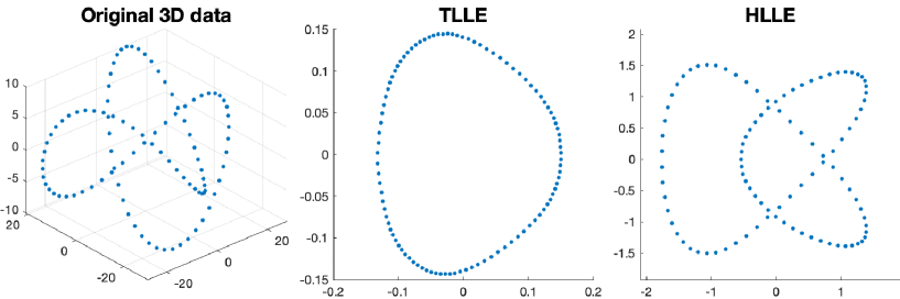
Figure 2: A comparison between TLLE and HLLE on the Trefoil knot.

Note that in this case, although the dimension of the manifold is one, it can not be embedded in the real line. We see that TLLE realizes the knot as a topological circle, while HLLE projects (possibly with some distortion) the knot onto the plane, causing self-intersections.

Figure 3 shows another illustrative example.

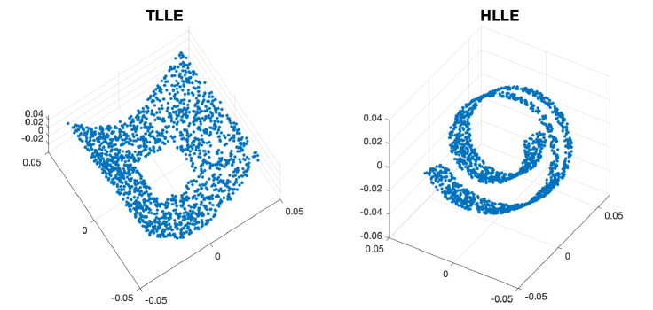
Figure 3: Results of TLLE and HLLE on the Swiss roll with a hole that is isometrically embedded in $\mathbb{R}^{9}$, and then mapped back to $\mathbb{R}^{3}$.

It is obtained by first performing an isometrical embedding of the Swiss roll with a hole in $\mathbb{R}^{9}$, and then – suppose we do not know that it can be well unfolded on the plane – applying TLLE and HLLE to map it back to $\mathbb{R}^{3}$. From the knowledge of $d_{\mathcal{M}}=2$, TLLE is capable of identifying the intrinsic geometry, and unfolds the Swiss roll to some extent in $\mathbb{R}^{3}$. On the other hand, HLLE just performs some projection from $\mathbb{R}^{9}$ to $\mathbb{R}^{3}$. Usually the results are similar to the original 3D data and look not bad, while in a few cases they happen to be highly compressed along some direction and are not satisfactory.

5 Conclusion

In this paper we explained that HLLE can be viewed as implementing the same idea as LLE: Asking the dimension-reduced data $\{y_{i}\}_{i=1}^{N}\subset\mathbb{R}^{d}$ to satisfy the same local linear relations as the original data $\{x_{i}\}_{i=1}^{N}\subset\mathbb{R}^{D}$ as best as possible. The main differences lie in the following two points:

• HLLE only considers linear relations of the $d$-dimensional principal component for each neighborhood;

• HLLE exploits multiple (originally $d(d+1)/2$) linear relations for each neighborhood.

With these being clear, we proposed a simplification where the “Hessian estimator” was replaced by randomly constructed weight matrices. Moreover, when $d$ is greater than $d_{\mathcal{M}}$ (the dimension of the data manifold), HLLE may produce projection-like results. To avoid this problem we suggested that the $d$-dimensional principal component in (A) should be replaced by the $d_{\mathcal{M}}$-dimensional one, which represents the tangential component of the original data. Combining the above simplification and modification, we finally achieved a new LLE-type method which was named tangential locally linear embedding (TLLE). It is simpler and more robust than HLLE.

So far, our numerical experiments are focused on artificial datasets such as the Swiss roll with a hole, and the performances of TLLE look excellent. Whether it is also helpful in producing reliable results for real world data or data with noise is an important direction for future investigation.

References

- [1] Mikhail Belkin and Partha Niyogi. Laplacian eigenmaps for dimensionality reduction and data representation. Neural computation, 15(6):1373–1396, 2003.
- [2] David L. Donoho and Carrie Grimes. Hessian eigenmaps: Locally linear embedding techniques for high-dimensional data. Proceedings of the National Academy of Sciences, 100(10):5591–5596, 2003.
- [3] Liren Lin. Avoiding unwanted results in locally linear embedding: A new understanding of regularization. arXiv, 2108.12680, 2021.
- [4] Sam T. Roweis and Lawrence K. Saul. Nonlinear dimensionality reduction by locally linear embedding. Science, 290(5500):2323–2326, 2000.
- [5] Jianzhong Wang. Geometric structure of high-dimensional data and dimensionality reduction. Springer, 2012.
- [6] Qiang Ye and Weifeng Zhi. Discrete hessian eigenmaps method for dimensionality reduction. Journal of Computational and Applied Mathematics, 278:197–212, 2015.
- [7] Zhenyue Zhang and Jing Wang. Mlle: Modified locally linear embedding using multiple weights. In Advances in neural information processing systems, pages 1593–1600, 2007.