CrossLoc: Scalable Aerial Localization Assisted by Multimodal Synthetic Data

Abstract

We present a visual localization system that learns to estimate camera poses in the real world with the help of synthetic data. Despite significant progress in recent years, most learning-based approaches to visual localization target at a single domain and require a dense database of geo-tagged images to function well. To mitigate the data scarcity issue and improve the scalability of the neural localization models, we introduce TOPO-DataGen, a versatile synthetic data generation tool that traverses smoothly between the real and virtual world, hinged on the geographic camera viewpoint. New large-scale sim-to-real benchmark datasets are proposed to showcase and evaluate the utility of the said synthetic data. Our experiments reveal that synthetic data generically enhances the neural network performance on real data. Furthermore, we introduce CrossLoc, a cross-modal visual representation learning approach to pose estimation that makes full use of the scene coordinate ground truth via self-supervision. Without any extra data, CrossLoc significantly outperforms the state-of-the-art methods and achieves substantially higher real-data sample efficiency. Our code and datasets are all available at crossloc.github.io .

crossloc.github.io

Figure 1: Left. The proposed TOPO-DataGen workflow generates multimodal synthetic datasets over large scales using off-the-shelf geodata. Right. We present CrossLoc, a cross-modal visual representation learning method for absolute localization. It learns to predict scene coordinates via self-supervised geometric tasks and external labels such as semantics if available.

1 Introduction

Due to vulnerabilities in the reception of satellite positioning (GNSS) signals, on which aerial systems rely for navigation and controls, alternative methods are in demand for absolute large-scale localization. The dead-reckoning navigation systems have improved significantly in recent years; however, residual drift is always a challenge for long-term applications [24, 33]. In contrast, the availability of small and low-cost cameras has made them popular sensors for capturing information on the surrounding landscape. When features of a known environment are recognized in the captured images, these can be used to determine the absolute camera poses. Current state-of-the-art machine-learning-based methods for absolute localization [13, 15, 17, 45, 46, 58] show promising performance but typically focus on single-domain operation and on bespoke datasets collected for indoor or outdoor city street localization [40]. However, open-source datasets for positioning airborne platforms or workflows to generate geospatial learning data are scarce. This poses a severe barrier in adapting the algorithms to real-world aerial scenarios, as they typically require dense datasets consisting of accurately geo-referenced photos in the area of interest [29]. Developing inclusive datasets for real-life navigation around the globe and employing state-of-the-art visual algorithms for aerial applications can currently be considered economically and technically difficult, if not unfeasible.

In this work, we first present a synthetic data generation scheme called TOPO-DataGen (Figure 1, left), that leverages the topographic information to produce geo-referenced data with rich modalities for subsequent training. Given the designated camera poses, this scheme renders the simulated RGB images accompanied by 2D and 3D modalities such as semantics, scene coordinates, depth, and surface normal. In an area of interest with available geodata, one may adopt a stochastic sampling strategy such as Latin hypercube sampling (LHS) [25, 39] or use real geo-tagged photos to attain the camera viewpoints and create the corresponding synthetic labels. The real geo-tagged data can be designer sourced, such as data acquisition by drones or from crowd sourced campaigns [4, 5]. Our method hinges on the geospatial location of the camera viewpoint and traverses between reality and simulation smoothly.

To mitigate the data-scarcity issue for learning-based visual localization methods via sim-to-real transfer, we curated two large-scale benchmark datasets at [22] using the proposed data generation workflow on urban and natural sites. They are comprised of primarily synthetic data and a small fraction of accurately geo-tagged real data, with both sections containing dense 3D and semantic labels. Unlike the existing datasets focusing on localization in a single domain [29, 32, 49], the provided benchmark datasets showcase and evaluate the use of synthetic data to assist localization in the real world using significantly less real data.

In addition, we introduce a cross-modal visual representation learning approach CrossLoc (Figure 1, right) for absolute localization via scene coordinate regression. CrossLoc exploits the rich information contained in the scene coordinates through self-supervision to achieve improved performance. We start from the scene coordinate ground-truth to impose geometrically less complex pretext tasks such as depth estimation without any extra labels. The visual representations learned from the tightly-coupled tasks [43, 68, 69] jointly improve the downstream coordinate regression. We find that this approach consistently outperforms the state-of-the-art baselines in our benchmark.

Our main contributions are summarized as follows:

1. TOPO-DataGen: an open-source multimodal synthetic data generation tool tailored to aerial scenes.

2. Large-scale benchmark datasets for sim-to-real visual localization, including synthetic and real images with 3D and semantic labels on urban and natural sites.

3. CrossLoc: a cross-modal visual representation learning method via self-supervision for absolute localization, which outperforms the state-of-the-art baselines.

2 Related work

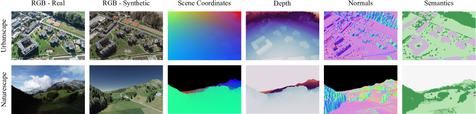
Figure 2: Examples of synthetic modalities generated with TOPO-DataGen. Our workflow traverses between the real and virtual world seamlessly hinged on the camera pose: from the leftmost real geo-tagged photos, we can generate a rich set of matching synthetic modalities, including synthetic RGB image, scene coordinates, depth, surface normal, and semantics.

Absolute visual localization aims at estimating the camera pose of a query image within a known environment. Many attempts have been made to achieve this using purely 2D images. Image retrieval [11, 12, 47, 59, 60] methods rely on the image features to build an explicit localization map. The query image is first matched against a database of reference images with known poses, and its pose w.r.t. to the retrieved image is subsequently refined via approximation or relative localization. Absolute pose regression [18, 30, 32, 64] approaches adopt a neural network to learn implicit map representations and output the camera pose directly.

Structure-based methods aim at identifying the 2D-3D matches between the query image pixels and the 3D coordinates of the scene model [13, 14, 15, 16, 17, 45, 46, 48, 58, 67, 70]. The camera pose can then be computed using a PnP solver with RANSAC optimization [17, 26, 35]. Compared with the 2D image-based approaches, the structure-based methods deliver more competitive performance [29, 46], but at the cost of attaining accurate 3D models for the underlying scenes, which is non-trivial and may require specialized engineering efforts [46]. The conventional descriptor matching methods, such as Active Search [48], typically create the 2D-3D correspondences via structure-from-motion (SfM) reconstruction and achieve state-of-the-art localization accuracy. However, the descriptor detector is prone to fail in repetitive or texture-less scenes or complex environments with entangling structures [56, 63].

Recently, the learning-based scene coordinate regression methods have been proposed [13, 14, 15, 16, 17, 37, 73] to predict the 2D-3D matches using neural networks in an end-to-end manner. Thanks to the great capacity of the neural network, it achieves state-of-the-art performance across various tasks [17]. The regressor learns from the ground-truth scene coordinates and can be theoretically separated from the SfM reconstruction. Most existing methods directly learn the mapping from image to coordinates while ignoring the rich geometry information contained in the 3D coordinate labels, $e.g.,$ one could compute camera pose and depth from scene coordinates given camera intrinsics.

Sim-to-real datasets have become increasingly important to tackle the issue of real data scarcity or to augment the real-world datasets during training. A set of synthetic datasets have been proposed and employed to facilitate model training for better robustness and efficiency [19, 23, 28, 42, 44, 52, 55, 61, 71]. [71] proposes the attend-remove-complete (ARC) method for sim-to-real depth prediction, which learns to identify, remove and fill in some challenging regions in real images as well as to translate the real images into the synthetic domain. Closer to our work, [23] provides a toolkit for mid-level cues generation from 3D models. However, it is not optimized for geodata and does not support synthetic data generation to match real geo-tagged photos. Likewise, most synthetic datasets or data generation workflows only involve rendered results in the virtual world and cannot traverse well between reality and simulation. Our proposed TOPO-DataGen workflow not only generates multimodal virtual data but can also produce georeferenced reality-matching data to intentionally augment the downstream learning tasks designed by the users.

3 TOPO-DataGen workflow

In this section, we describe the TOPO-DataGen toolkit for synthetic data generation as shown in Figure 1 (left).

Geodata preprocessing. In the first step, a high-fidelity 3D textured model is generated over the area of interest based on available geographic data, $e.g.,$ classified LiDAR point cloud, orthophoto, or digital terrain model. We preprocess the off-the-shelf geodata such that it is compatible with the open-source geospatial rendering engine CesiumJS [1], which is at the core of our data generation workflow. For example, one common practice is to convert the coordinate reference system into the global WGS84 from the local one. We argue that nowadays, the high-quality open geodata from national agencies is more and more common [20] such as the swisstopo [6, 7, 8], making it easier to access the 3D models for locations of interest and employ our method on a large scale. Moreover, the open geodata mostly comes from airborne devices such as satellites. Its accuracy and the top-down view are generally sufficient for aerial localization tasks as opposed to street-level localization.

Synthetic data generation. The generated 3D textured model in the WGS84 reference system is the input to CesiumJS engine for synthetic data generation. Given the virtual camera viewpoint, our proposed TOPO-DataGen provides a series of designer modalities related to visual localization, which include: RGB image, scene coordinates in the WGS84 reference system ($i.e.,$ earth-centered-earth-fixed coordinates), depth, surface normal, and semantics. Specifically, through ray tracing [10], our workflow produces synthetic RGB images and the geo-referenced scene coordinates as raw output. Subsequently, we retrieve the semantic maps by matching each pixel to its closet point in the categorized geodata, $i.e.$, the classified LiDAR point cloud. The PyTorch [41] framework is used to accelerate the matrix computation. Lastly, based on the scene coordinate labels, we generate the other 3D modalities, $i.e.$, depth and surface normal. Following [69], we provide the z-buffer depth, and the surface normal is computed using Open3D [74].

The data rendering can be performed offline over a large area, the size of which is limited by the computer hardware and the available geodata. To generate synthetic data from scratch, $e.g.,$ to scan one bounded area, we use the LHS [25, 39] to do minimal yet efficient camera viewpoints sampling. Otherwise, one may use any real geo-tagged photos to generate the matching synthetic modalities as shown in Figure 2 (from the leftmost to the right).

Quality control. The quality of the multimodal synthetic data is essentially dependent on the precision of the 3D model geo-referencing and the accuracy of the image pixel-scene coordinate ray tracing. Please see the supplement for a detailed case study on the provided benchmark datasets (introduced in Section 4).

4 Benchmark datasets

We introduce two large-scale sim-to-real benchmark datasets to exemplify the utility of the TOPO-DataGen.

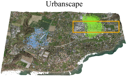
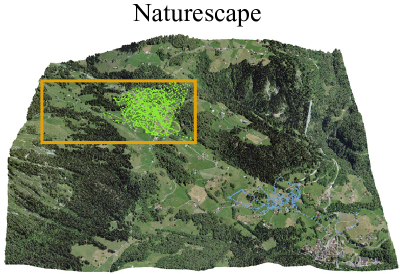
Figure 3: 3D textured models used to render the benchmark datasets with synthetic modalities via LHS sampling or matching the real flight trajectories. Camera positions of in-place and out-of-place data are colored in green and blue respectively, and the LHS synthetic data sampling boundary is denoted by the orange box.

Landscape	Scene	Size	Image style	Area
Urbanscape	LHS-sim	15000	Sim only	45.8ha
	In-place	3158	Real-Sim pairs	40.4ha
	Out-of-place	1360	Real-Sim pairs	46.6ha
Naturescape	LHS-sim	30000	Sim only	128.25ha
	In-place	2114	Real-Sim pairs	107.5ha
	Out-of-place	565	Real-Sim pairs	49.7ha

Table 1: Benchmark datasets statistics.

Dataset statistics. Table 1 shows the statistics of the benchmark datasets, which are distributed across two different landscapes: Urbanscape and Naturescape. For each landscape, we provide data in three scenes: LHS-sim, In-place and Out-of-place, all of which come with synthetic 2D images, multimodal 3D labels and semantic map as depicted in Figure 2. Specially, the In-place and Out-of-place scenes include accurately geo-tagged real photos captured by a DJI Phantom 4 drone equipped with the cm-level real-time kinematics (RTK) positioning. [2]. The In-place scene is highly overlapped with the LHS-sim scene, while the Out-of-place scene describes a neighboring but non-overlapping environment w.r.t LHS-sim. Figure 3 shows the 3D textured models with camera position distributions of the datasets.

In the proposed datasets, the data resolution for all modalities, including real and synthetic images, is set to 480 px in height and 720 px in width. The semantic labels have seven classes: sky, ground, vegetation, building, water, bridge, and others. Following [29], we evaluate the accuracy of the synthetic 3D labels by coordinate reprojection error. The mean absolute reprojection error of the Urbanscape and Naturescape datasets are respectively 1.19 px and 1.04 px, showing high accuracy for outdoor aerial datasets. More error analysis can be found in the supplement.

Dataset splits. We randomly split the In-place and Out-of-place scene data into training (40%), validation (10%) and testing (50%) sections. As for the LHS-sim scene data, it is split into training (90%) and validation (10%) sets. We intentionally formulate a challenging visual localization task by using more real data for testing than for training to better study the real data scarcity mitigation. Please also note that the real image density indicated in Table 1 is lower than many available outdoor city street-based visual localization datasets such as Cambridge [32] and Aachen [49, 50].

5 CrossLoc localization

In this section, we present CrossLoc, an absolute localization algorithm leveraging the cross-modal visual representations for enhanced robustness and data efficiency. CrossLoc learns to localize the query image by predicting its scene coordinates using a set of cross-modal encoders, followed by camera pose estimation using a PnP solver.

Coordinate-depth-normal geometric hierarchy. For an image $\mathcal{I}$ with ground-truth scene coordinates $\mathcal{Z}$ and camera pose $(\mathcal{R,P})\in\mathbb{SE(3)}$ in the world coordinate system, it is straightforward to compute the Euclidean or z-buffer depth $\mathcal{D}$ via homogeneous transformation. Subsequently, the surface normal $\mathcal{N}$ can be obtained from the depth map $\mathcal{D}$ [43, 74]. The geometrical information richness of the scene coordinates $\mathcal{Z}$ label is beyond that of depth $\mathcal{D}$ and surface normal $\mathcal{N}$, as one can convert the first to the latter without loss of accuracy.

We hypothesize that if a neural network is capable of predicting perfect scene coordinates $\mathcal{Z}$, it possesses sufficient information to estimate high quality depth $\mathcal{D}$ and surface normal $\mathcal{N}$. Inspired by the natural geometric hierarchy, we propose to learn scene coordinate regression with auxiliary self-supervision tasks on depth and surface normal estimation. Our method is modular and also extends to using any external labels such as semantics $\mathcal{S}$ if they may be available.

Consider an encoder-decoder network making predictions $\mathcal{T}_{q}\in\{\mathcal{Z}_{q},\mathcal{D}_{q},\mathcal{N}_{q}\}$ from a query image $\mathcal{I}_{q}$. Let $f^{\mathcal{T}}(\cdot),g^{\mathcal{T}}(\cdot),h^{\mathcal{T}}$ denote the encoder, decoder and the mid-way representations respectively:

$$\begin{split}h^{\mathcal{T}}_{q}&=f^{\mathcal{T}}(\mathcal{I}_{q}),\\ \hat{\mathcal{T}}_{q}&=g^{\mathcal{T}}(h^{\mathcal{T}}_{q}).\end{split}$$ (1)

where $\hat{\mathcal{T}}_{q}$ is the network prediction. Based on the coordinate-depth-normal geometric hierarchy, we argue that the representations for scene coordinate $h^{\mathcal{Z}}_{q}$ may encode richer information than the others, $e.g.,$ $h^{\mathcal{D}}_{q},h^{\mathcal{N}}_{q}$.

To better ensure the hierarchical consistency, we propose to explicitly learn a cross-modal scene coordinate regression representation $h^{\mathcal{Z}}_{q}$ with those of lower-level tasks:

$$h^{\mathcal{Z}_{+}}_{q}=f^{\mathcal{Z}_{+}}(h^{\mathcal{Z}}_{q},h^{\mathcal{D}}_{q},h^{\mathcal{N}}_{q}).$$ (2)

where $f^{\mathcal{Z}_{+}}$ is a projection head for representations aggregation. Next, the cross-modal representation is fed into the primary task decoder for scene coordinate regression:

$$\hat{\mathcal{Z}}^{+}_{q}=g^{\mathcal{Z}}(h^{\mathcal{Z}_{+}}_{q}).$$ (3)

Afterward, the 6D camera pose could be computed using the coordinates prediction via a PnP solver, as per the standard scene coordinate regression localization methods.

Training objective. Let $N$ be the number of pixels in the image. We use azimuth $\theta$ and elevation $\phi$ to represent the surface normal vectors as in [36], and therefore: $\mathcal{Z}\in\mathbb{R}^{N\times 3},\mathcal{D}\in\mathbb{R}^{N\times 1},\mathcal{N}=[\mathcal{N}^{\theta},\mathcal{N}^{\phi}]\in\mathbb{R}^{N\times 2}$. The maximum likelihood estimation loss [31, 73] is used to stabilize the coordinate, depth and surface normal regression training. The predicted values come with isotropic noise estimation: $[\hat{\mathcal{T}},s^{\mathcal{T}}]=g^{\mathcal{T}}(h^{\mathcal{T}})$, where $s^{\mathcal{T}}\in\mathbb{R}^{N\times 1}_{>0}$ is the pixel-wise uncertainty map. We adopt a two-step training method to regularize the scene coordinate representations $h^{\mathcal{Z}_{+}}$. First, the encoder-decoders $f^{\mathcal{T}},g^{\mathcal{T}}$ ($\mathcal{T}\in\{\mathcal{Z},\mathcal{D},\mathcal{N}\}$) are separately trained with their own loss functions:

$$\begin{split}\small L_{\mathcal{Z}}&=\sum_{i=1}^{N}\left(\frac{\|\hat{\mathcal{Z}}(i)-\mathcal{Z}(i)\|^{2}_{2}}{2(s^{\mathcal{Z}}(i))^{2}}+3\text{ log}(s^{\mathcal{Z}}(i))\right),\\ L_{\mathcal{D}}&=\sum_{i=1}^{N}\left(\frac{\|\hat{\mathcal{D}}(i)-\mathcal{D}(i)\|^{2}_{2}}{2(s^{\mathcal{D}}(i))^{2}}+\text{log}(s^{\mathcal{D}}(i))\right),\\ L_{\mathcal{N}}&=\sum_{i=1}^{N}\left(\frac{\|L_{sn}(\hat{\mathcal{N}}(i),\mathcal{N}(i))\|^{2}_{2}}{2(s^{\mathcal{N}}(i))^{2}}+2\text{ log}(s^{\mathcal{N}}(i))\right).\end{split}$$ (4)

where

$$\begin{split}L_{sn}(\hat{\mathcal{N}}(i),\mathcal{N}(i))&=\|\hat{\mathcal{N}}^{\phi}(i)-\mathcal{N}^{\phi}(i)\|_{1}+\\ 2\text{ min}&\left(\|\hat{\mathcal{N}}^{\theta}(i)-\mathcal{N}^{\theta}(i)\|_{1},1-\|\hat{\mathcal{N}}^{\theta}(i)-\mathcal{N}^{\theta}(i)\|_{1}\right)\end{split}$$

is the circle loss defined in [36]. The subscript in Eq. (4) denotes the loss function for the corresponding task $\mathcal{T}$. Following [17], we also implement the reprojection loss for coordinate regression loss $L_{\mathcal{Z}}$.

Lastly, we employ the non-coordinate encoders as frozen representation extractors to fine-tune the coordinate encoder-decoder $f^{\mathcal{Z}},g^{\mathcal{Z}}$ and the projection head $f^{\mathcal{Z}_{+}}$:

$$L_{crossloc}=L_{\mathcal{Z}}(f^{\mathcal{Z}},g^{\mathcal{Z}},f^{\mathcal{Z}_{+}}).$$ (5)

The CrossLoc applies the multi-task learning by re-using the representations of geometrically-related tasks to improve the original objective of coordinate regression. Table 2 shows some variants of the proposed methods, among which the vanilla CrossLoc adopts the self-supervised cross-modal representation learning without any additional data. Our method is flexible with external labels such as semantics, e.g., the CrossLoc-SE.

Encoders	CrossLoc	CrossLoc-SE	CrossLoc-CO
Coordinate	✓	✓	✓
Depth	✓	✓
Surface normal	✓	✓
Semantics		✓

Table 2: Variants of the proposed CrossLoc algorithm.

6 Experiments

Extensive experiments have been carried out to evaluate the performance of CrossLoc against the state-of-the-art approaches to scene coordinate regression. Specifically, we apply various CrossLoc architectures in Table 2 to validate the effectiveness of self-supervision. Systematic ablation studies about the efficacy of synthetic training data on real data scarcity mitigation are also conducted.

Network architecture. Following [17], we adopt a fully convolutional network (FCN) with ResNet skip layers [27] for regression tasks using a downsampling factor of 8. We split the FCN in the middle to obtain an encoder-decoder structure. Please refer to the supplement for further details.

Datasets. Each model is trained using data from the LHS-sim and either In-place or Out-of-place scene. We evaluate on the real testing data for each scene and report the results.

Training. We first initialize the encoder-decoder networks separately using various training tasks on the LHS-sim data; subsequently, each network is fine-tuned with the paired real-sim data on either In-place or Out-of-place scene. Each network is independently trained using the loss in Eq. (4). Lastly, we fine-tune the coordinator network with loss in Eq. (5). For CrossLoc-SE, we use the cross-entropy loss for semantic segmentation. We use the Adam optimizer [34] and the PyTorch [41] framework for implementation.

Baselines. We compare our proposed algorithms against two state-of-the-art scene coordinate regression baselines: DSAC* [17] and sim-to-real coordinate regression DDLoc adapted from [71]. We follow the ARC [71] architecture to train a regressor for coordinates instead of depth with minimum modification; see the supplement for details. For a fair comparison, all the coordinate regression-based approaches utilize the PnP solver from DSAC* [17] to compute camera poses. Also, our method is compared with AtLoc [64], a state-of-the-art absolute pose regression (APR) method. Please note that AtLoc does not use any 3D labels and has much less information to learn from during training.

6.1 Results on camera pose estimation

	In-place localization accuracy					Out-of-place localization accuracy
Methods	Median error $\downarrow$		Accuracy $\uparrow$			Median error $\downarrow$		Accuracy $\uparrow$
	transl.	rot.	$<$ 5m, 5°	$<$ 10m, 7°	$<$ 20m, 10°	transl.	rot.	$<$ 5m, 5°	$<$ 10m, 7°	$<$ 20m, 10°
DSAC* [17]	11.6m	6.2°	15.4%	42.1%	64.4%	14.9m	4.1°	10.3%	33.1%	59.6%
DDLoc	10.3m	2.3°	24.1%	47.2%	67.8%	42.1m	9.5°	4.1%	12.8%	26.5%
AtLoc [64]	23.0m	1.9°	1.6%	11.1%	40.6%	45.6m	5.3°	0.1%	2.4%	14.1%
CrossLoc	4.0m	2.1°	61.1%	85.6%	93.4%	6.0m	1.9°	39.1%	72.4%	87.8%
CrossLoc-SE	3.9m	1.9°	62.2%	86.7%	94.2%	5.8m	1.8°	40.1%	73.4%	89.1%
CrossLoc-CO	7.6m	3.7°	27.6%	61.3%	80.5%	7.1m	2.2°	31.5%	64.9%	82.8%

(a) Quantitative comparison over Urbanscape dataset.

	In-place localization accuracy					Out-of-place localization accuracy
Methods	Median error $\downarrow$		Accuracy $\uparrow$			Median error $\downarrow$		Accuracy $\uparrow$
	transl.	rot.	$<$ 5m, 5°	$<$ 10m, 7°	$<$ 20m, 10°	transl.	rot.	$<$ 5m, 5°	$<$ 10m, 7°	$<$ 20m, 10°
DSAC* [17]	41.9m	4.8°	1.8%	11.3%	30.1%	33.1m	4.3°	0.4%	6.7%	26.5%
DDLoc	39.8m	4.2°	2.2%	10.9%	28.0%	57.4m	8.2°	2.5%	12.0%	22.6%
AtLoc [64]	44.7m	5.1°	0.0%	1.5%	10.7%	70.8m	6.6°	0.0%	0.0%	2.5%
CrossLoc	16.7m	2.9°	9.6%	28.4%	59.6%	15.0m	2.7°	8.1%	29.7%	59.0%
CrossLoc-SE	16.0m	2.7°	11.4%	32.6%	59.7%	14.5m	2.2°	12.7%	32.5%	59.4%
CrossLoc-CO	22.6m	3.8°	6.2%	20.1%	42.5%	17.1m	2.9°	7.1%	29.0%	55.5%

(b) Quantitative comparison over Naturescape dataset.

Table 3: Quantitative results on camera pose estimation. We report the median translation and rotation errors as well as the percentage of correctly re-localized camera poses below error thresholds of 5m/5°, 10m/7°and 20m/10°.

Figure 4: Qualitative comparison of the reconstructed trajectories with the studied visual localization methods. We show the results for a planned trajectory on Naturescape and a human-piloted trajectory on Urbanscape, both derived from the testing data. The rightmost color bar denotes the camera position estimation error in meter.

Quantitative results. Table 3 lists detailed comparisons for pose estimation on Urbanscape and Naturescape datasets. CrossLoc outperforms the other two coordinate regression methods by a clear margin, demonstrating the superior performance of cross-modal representation learning. Notably, the 2D image-based APR baseline AtLoc [64] shows inferior performance to any of the structure-based methods. This is not unexpected as the APR tends to generalize worse from the training data in practice [51]. We also provide the results of our CrossLoc algorithm using different visual representations, $i.e.,$ CrossLoc-CO applying only coordinate regression features and CrossLoc-SE using additional semantic segmentation features (see Table 2). Adding the auxiliary depth and surface normal visual features substantially boosts the model performance. However, CrossLoc-SE with external semantic labels has limited performance gains compared with the vanilla CrossLoc. This indicates incorporating additional labels with less geometrical information may not help the scene coordinate learning prominently. This finding is also in line with the recent works on multi-task learning consistency [43, 57, 68, 69]. The localization accuracy in the Naturescape is not as high as in the Urbanscape. We conjecture that this is due to the lower amount of human-made features with distinctive geometries such as buildings. Moreover, the much lower real training data density, as stated in Table 1, makes the localization task considerably harder.

Qualitative results. Figure 4 shows the pose estimation results of two flight trajectories in the Naturescape and Urbanscape datasets respectively. Our CrossLoc outperforms other localization algorithms, resulting in far more complete trajectory reconstruction with much fewer outliers.

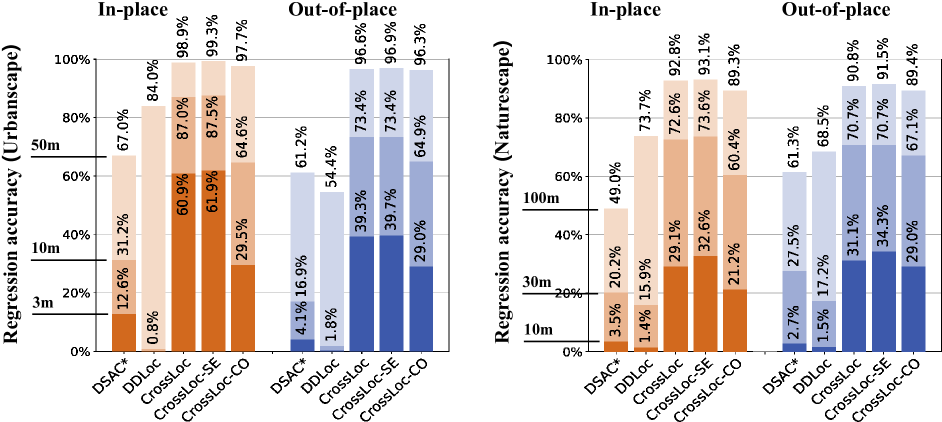
Figure 5: Percentage of correctly predicted scene coordinates with different methods. The accuracy is represented with error thresholds, 3m, 10m and 50m for Urbanscape as well as 10m, 30m and 100m for Naturescape. Only two accuracy values of DDLoc are given in Urbanscape since there is nearly no predicted coordinate with error lower than 3m.

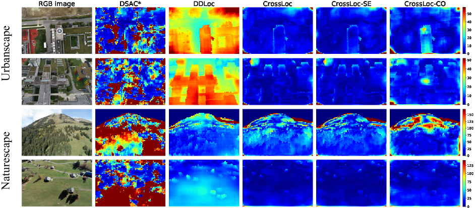
Figure 6: Qualitative comparison of the scene coordinate error map. Pixels without groundtruth labels such as sky are not evaluated. Our CrossLoc family methods estimate the absloute scene coordinates with the least error.

6.2 Results on scene coordinates regression

Quantitative results. For coordinate regression-based localization methods, the final pose estimation performance is highly dependent on the coordinate prediction quality. Figure 5 shows the accuracy of regressed scene coordinates under different thresholds. Consistent with the pose estimation results in Table 3, the CrossLoc architecture frameworks outperform the DSAC* and DDLoc baselines by a substantial margin. Moreover, CrossLoc and CrossLoc-SE improve the coordinate accuracy over CrossLoc-CO across all scenarios, which further indicates the benefit of leveraging depth and surface normal cross-modal representations.

Qualitative results. Figure 6 compares the scene coordinate regression errors of different methods. The regression error of our CrossLoc and CrossLoc-SE is significantly lower than the baselines and the plain CrossLoc-CO without self-supervision. Further, we observe a high similarity between the error map of CrossLoc and CrossLoc-SE, which shows limited performance gains by using the extra semantic labels. For discussion on the failure cases, please refer to the supplementary materials.

6.3 Ablation study on real data scarcity mitigation

Methods	Localization accuracy w.r.t. amount of synthetic data
	Real only	Pairwise only	Full
DSAC* [17]	35.5m, 17.7°	23.7m, 12.1°	11.6m, 6.2°
DDLoc	-	11.0m, 2.8°	10.3m, 2.3°
CrossLoc	7.6m, 3.6°	4.6m, 2.4°	4.0m, 2.1°
CrossLoc-CO	14.6m, 7.0°	12.8m, 6.2°	7.6m, 3.7°

(a) Effects of synthetic data assisting the real-world localization.

Methods	Localization accuracy w.r.t. fraction of pairwise data
	25% data	50% data	Full
DSAC* [17]	33.1m, 17.6°	19.4m, 10.2°	11.6m, 6.2°
CrossLoc	14.1m, 7.1°	6.8m, 3.5°	4.0m, 2.1°
CrossLoc-CO	28.3m, 13.7°	13.7m, 6.3°	7.6m, 3.7°

(b) Comparison of real data sample efficiency.

Table 4: Ablation study on the real data scarcity mitigation. Median translation and rotation error is reported.

We show the quantitative results on how the real data scarcity issue can be mitigated by: (i) using the synthetic data for augmentation, which could be generated at ease using the proposed TOPO-DataGen, (ii) applying the real data sample-efficient CrossLoc algorithm. All experiments in this section are carried out on Urbanscape in-place scene.

The added value of the multimodal synthetic data is validated in Table 4(a). We compare the performance of various methods trained with real data only, real-sim paired data only, and real-sim paired data plus the plentiful LHS-sim data. For each method, the best performance is always achieved with the most synthetic data. CrossLoc consistently performs the best, which indicates the usefulness of the proposed self-supervision via geometric hierarchy.

In Table 4(b), we evaluate the real data sample efficiency of different methods, assuming that the paired synthetic data is available. We randomly sample 25% and 50% of the real training data to train each model. Each algorithm performs better given a larger amount of training data, and in comparison, the CrossLoc leverages the real data most efficiently. CrossLoc outperforms the 100%-data-trained DSAC* and all CrossLoc-CO when trained with only 50% of available data. The proposed geometrical self-supervision tasks are particularly helpful for learning in the low-data regime.

7 Conclusion

We propose TOPO-DataGen, a scalable workflow to generate as much synthetic data as needed to assist real-world localization. Large-scale sim-to-real benchmark datasets are additionally provided to exemplify the use of TOPO-DataGen. Further, we present CrossLoc that learns to predict coordinates and localize via geometric self-supervision. It significantly outperforms the state-of-the-art baselines in our benchmark, especially in the low-data regime. We believe that TOPO-DataGen, altogether with CrossLoc, could open up new opportunities for large-scale aerial localization applications in the real world.

Appendix

Appendix A Benchmark datasets error analysis

We validate the accuracy of the multimodal synthetic data generated through our TOPO-DataGen and the geo-tag quality of the real images captured by our drone [2] equipped with the real-time kinematics (RTK) level of Global Navigation Satellite System (GNSS) positioning.

A.1 Synthetic data quality control

Geo-referenced 3D scene model precision. For the whole benchmark datasets, the digital surface models (DTM) [8] and the LiDAR point clouds [7] used for rendering were acquired with planimetric precision of $\pm$ 20 cm and altimetric precision of $\pm$ 10 cm. We employ the orthophoto assets with a position accuracy of $\pm$ 15 cm and a resolution of 10 cm [6] to colorize the DTM and point clouds. The $\pm$ sign denotes the standard deviation w.r.t. the local coordinate reference systems [3]. In the pre-processing step, we convert the open geodata into the global WGS84 coordinate reference system, and the loss of accuracy therein is negligible. Please see our source code for more details.

	Urbanscape		Naturescape
	transl.	rot.	transl.	rot.
Mean	0.11m	0.06°	0.23m	0.06°
Std.	0.06m	0.03°	0.09m	0.03°
Median	0.10m	0.06°	0.22m	0.06°

Table 5: Indirect quality estimation of the scene coordinate labels. We feed the generated coordinate maps into the DSAC* [17] PnP solver and compute the poses error w.r.t. the ground truth camera viewpoints.

	Urbanscape	Naturescape
Mean	1.19px	1.04px
Std.	0.16px	0.11px
Median	1.14px	1.03px
90%	1.44px	1.08px
95%	1.52px	1.09px
99%	1.68px	1.14px

Table 6: Absolute reprojection error of the scene coordinate labels. Following [29], we report the reprojection error in the image plane in pixels and particularly show the percentile errors to indicate the long tail distribution.

Scene coordinate ray tracing accuracy. The ray-traced scene coordinate label accuracy is further evaluated by verifying the camera pose computation. Table 5 demonstrates how well the generated coordinate maps correspond to the ground truth virtual camera viewpoints. The mean camera pose computation errors for the Urbanscape and Naturescape datasets are 0.11m, 0.06°, and 0.23m, 0.06°, respectively. We use the eight-times-downsampled scene coordinates in this evaluation, the same dataset used in the main paper’s experiments.

Table 6 reports the reprojection error of the scene coordinates w.r.t. to the ground-truth camera viewpoints as in [29]. The proposed benchmark datasets have consistently low error at the magnitude of one or two pixels in both scenes. The percentile errors are close to the mean or median errors and indicate that there are few occurrences far away from the central distribution. The full-size coordinate maps (without downsampling) are used in the reprojection error analysis.

A.2 Real data quality control

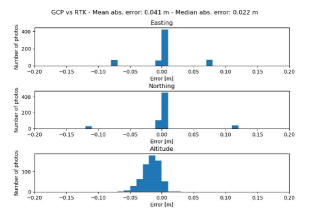
(a) Urbanscape RTK precision: position error.

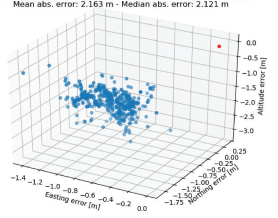
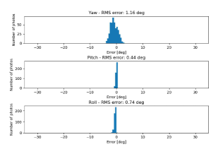
(b) Naturescape RTK precision. Left. Position error. Right. Orientation error.

Figure 7: Accuracy evaluation of the real data RTK geo-tag. We show the camera pose refinement error obtained by solving the photogrammetry bundle adjustment via GCP alignment. The RTK precision in the Urbanscape dataset is at cm level, while it degrades to over 2 meters in the Naturescape dataset because of weak GNSS signals.

To collect high-accuracy aerial photos, a DJI Phantom 4 RTK drone [2] was used, whose RTK positioning enables a cm-level accuracy for the image geo-tags. A network of ground control points (GCP) was measured with a JAVAD Triumph-LS [9] base with mm-level accuracy. We use 13 and 6 GCPs, respectively, for the Urbanscape and the Naturescape datasets to solve the bundle adjustment photogrammetric alignment and compare with the RTK geo-tags extracted from the photo metadata. Figure 7 shows the RTK geo-tag error statistics w.r.t. the computed photogrammetry ground truth. The geo-tag precision at the Urbanscape dataset is as small as 4 cm, while it degrades significantly in the Naturescape dataset.One can observe that there is a mean positional error bias. In the next steps, this bias was subtracted for all images of each drone, bringing the error to a lower level (mean error = 0.42 m).

Appendix B Potential societal impact

TOPO-DataGen and benchmark datasets. The proposed TOPO-DataGen is a multi-purpose task-agnostic synthetic data generation tool that entails little ethical concerns. Essentially, it needs real-world geo-data to perform data rendering, most of which is provided by national agencies [20]. The incoming researchers adopting our method are advised to pay attention to the privacy or transparency of the underlying geo-data before implementation. In our benchmark datasets, the open-source swisstopo [6, 7, 8] geo-data is employed for synthetic data generation, and the real data is collected using a drone. The produced images and associated labels have airborne perspectives, distinct from those in indoor or urban street scenes. There is no human object data or personally identifiable information in our datasets.

CrossLoc localization. Our CrossLoc is a scene coordinate regression-based localization method and does not impose particular requirements infringing privacy. It learns to localize the image primarily based on the distinct geometries in the environment, such as mountains or buildings. It does not require human data and is unlikely to benefit from any.

Appendix C Implementation details

C.1 CrossLoc architecture

	Urbanscape						Naturescape
Task	Encoder pretraining		Encoder finetuning		Encoder finetuning		Encoder pretraining		Encoder finetuning		Encoder finetuning
			with in-place data		with out-of-place data				with in-place data		with out-of-place data
	Epoch	Initial LR	Epoch	Initial LR	Epoch	Initial LR	Epoch	Initial LR	Epoch	Initial LR	Epoch	Initial LR
Coordinate	150	0.0002	150	0.0002	1500	0.0002	100	0.0002	150	0.0002	2000	0.0002
Depth	150	0.0002	150	0.0002	300	0.0002	100	0.0002	150	0.0002	2000	0.0002
Surface normal	150	0.0002	150	0.0002	300	0.0002	100	0.0002	150	0.0002	2000	0.0002
Semantics	30	0.0002	30	0.0002	30	0.0002	30	0.0002	30	0.0002	30	0.0002

Table 7: CrossLoc encoder-decoder initialization training hyper-parameters.

Layer	Channel I/O	Kernel/Str./Pad.	Input
conv1	3/32	3/1/1	image
conv2	32/64	3/2/1	conv1
conv3	64/128	3/2/1	conv2
conv4	128/256	3/2/1	conv3
res1_conv1	256/256	3/1/1	conv4
res1_conv2	256/256	1/1/0	res1_conv1
res1_conv3	256/256	3/1/1	res1_conv2
res2_add	-/-	-/-/-	relu(res1_conv3+conv4)
res2_conv1	256/512	3/1/1	res2_add
res2_conv2	512/512	1/1/0	res2_conv1
res2_conv3	512/512	3/1/1	res2_conv2
res2_conv_s	256/512	1/1/0	res2_add
res3_add	-/-	-/-/-	relu(res2_conv3+res2_conv_s)
res3_conv1	512/512	3/1/1	res3_add
res3_conv2	512/512	1/1/0	res3_conv1
res3_conv3	512/512	3/1/1	res3_conv2
res4_add	-/-	-/-/-	relu(res3_conv3+res3_add)
res4_conv1	512/512	3/1/1	res4_add
res4_conv2	512/512	1/1/0	res4_conv1
res4_conv3	512/512	3/1/1	res4_conv2
feat_enc	-/-	-/-/-	relu(res4_conv3+res4_add)

(a) Encoder architecture.

Layer	Channel I/O	Kernel/Str./Pad.	Input
res1_conv1	512/512	3/1/1	feat_dec
res1_conv2	512/512	1/1/0	res1_conv1
res1_conv3	512/512	3/1/1	res1_conv2
res2_add	-/-	-/-/-	relu(res1_conv3+feat_dec)
res2_conv1	512/512	3/1/1	res2_add
res2_conv2	512/512	1/1/0	res2_conv1
res2_conv3	512/512	3/1/1	res2_conv2
res3_add	-/-	-/-/-	relu(res2_conv3+res2_add)
res3_conv1	512/512	1/1/0	res3_add
res3_conv2	512/512	1/1/0	res3_conv1
res3_conv3	512/512	1/1/0	res3_conv2
fc1	512/512	1/1/0	relu(res3_conv3+res3_add)
fc2	512/512	1/1/0	fc1
output	512/$N$	1/1/0	fc2

(b) Decoder architecture.

Layer	Channel I/O	Kernel/Str./Pad.	Input
feat_add	-/-	-/-/-	feat_enc_1 $\bigoplus$ $\cdots$ $\bigoplus$ feat_enc_T
feat_conv1	512$T$/512	3/1/1	feat_add
feat_conv2	512/512	1/1/0	feat_conv1
feat_conv3	512/512	3/1/1	feat_conv2
feat_skip	512$T$/512	1/1/0	feat_add
feat_cat	-/-	-/-/-	relu(feat_conv3 + feat_skip)

(c) Representation projection head architecture.

Table 8: CrossLoc network architecture.

Network architecture. Following [17], we adopt a fully convolutional network with ResNet-style skip layers [27] to employ the diverse data augmentation, including rescaling and rotation. Table 8 shows the CrossLoc encoder-decoder network and the projection head for representations concatenation. We apply group normalization [66] and relu nonlinear activation function for each convolutional or residual layer. The parameter $N$ in Table 8(b) is task dependent, $e.g.$, for coordinate regression $N=4$ because of 3-dimensional coordinate prediction and 1-dimensional uncertainty estimation. The parameter $T$ in Table 8(c) refers to the number of visual representations; for the vanilla CrossLoc, $T=3$, and for the CrossLoc-SE using external semantics, $T=4$. The sign $+$ and $\bigoplus$ respectively stand for addition and channel-wise concatenation operators. As in [17], we use consecutive three convolutional layers with strides of two to downsample the prediction eight times. For the semantic segmentation task, we keep the full-size labels and apply the dense upsampling convolution [65] in the final output layer to recover the full-size semantic prediction.

Training hyper-parameters. In the first step of CrossLoc training, we pretrain the sub-task networks with task-agnostic LHS-sim synthetic data, and fine-tune the models with pairwise real-sim data. Table 7 shows the specific training hyper-parameters. The learning rate is halved at 50 and 100 epochs at most twice. We extend the encoder fine-tuning epochs particularly on the out-of-place scene in both datasets to ensure convergence. Notably, the semantic segmentation tasks reach convergence much faster than the other regression tasks. Subsequently, during coordinate network fine-tuning using the frozen non-coordinate encoders as feature extractors, we train each model for 1000 epochs with a fixed learning rate of 0.0001. In line with [54, 71], we find that reusing fixed modules instead of training from scratch simultaneously improves training convergence. The Adam optimizer [34] is used throughout our training.

C.2 DDLoc architecture

ARC structure. DDLoc is our adaption of the attend-remove-complete (ARC) framework [71], which is a state-of-the-art domain transformation method. The original ARC architecture contains a style translator mapping images between real-world and synthetic domains. It further trains an attention module to detect challenging regions and an inpainting module to complete the masked regions with realistic fill-in. A depth predictor module then takes the translated result as input to make the prediction. The ARC method has been verified by extensive experiments that it can leverage synthetic data for accurate depth estimations [71].

Network architecture. In our implementation of DDLoc, the depth predictor is replaced with a coordinate regressor, which is implemented by an encoder-decoder architecture [75] with skip connections [72]. Based on that, the scene coordinate prediction is further down-sampled by the factor of 8 to enhance efficiency as well as to increase the receptive field [17]. The down-sampling is implemented by fully convolution layers with stride of 2. Any other single module in DDLoc uses the same encoder-decoder architecture as used in [75]. The decoder of the attention module is modified to output a single channel to discover challenging regions from real-world input images.

Training hyper-parameters. Following ARC’s training method [71], we first pretrain each module individually using the Adam optimizer [34] with an initial learning rate of 0.0001 and coefficients of 0.9 and 0.999. For training the coordinate regressor, we adapt the original depth loss for the coordinate regression distance, and employ re-projection loss as in DSAC* [17]. The sparsity level $\rho$ is chosen as 0.9 when training the attention module on the Urbanscape and the Naturescape datasets. Other modules are trained with the same loss as that in the original ARC implementation. Lastly, we fine-tune the whole framework with the loss of the coordinate predictor pretraining and the same training parameters.

Appendix D Additional qualitative results and analysis

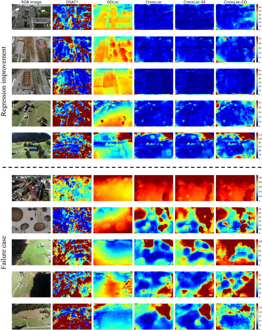
Figure 8: Additional qualitative comparison of the scene coordinate error map including improvement and failure cases. We use the same color bar for visualizing coordinate regression error in each row with the unit in meter.

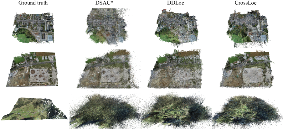
Figure 9: Comparison of point clouds predicted by different coordinate regression approaches. Our CrossLoc method generates a more complete and robust reconstruction of the buildings than the other two baselines.

In this section, we visualize additional comparisons of the scene coordinate regression errors in Figure 8 and compare the predicted point clouds of several urban and natural scenarios in Figure 9. We show examples where our CrossLoc outputs accurate coordinate prediction and failure cases where it makes much worse estimation. Eventually, we summarize the technical limitations of our proposed methods.

Failure cases. Generally, CrossLoc and its variants outperform the others by a clear margin. Nevertheless, there are two exceptional cases where the CrossLoc family cannot make a good prediction. First, novel objects, such as construction cranes, are challenging to the CrossLoc. We conjecture that CrossLoc learns the geometric information of the buildings as a whole. Thus, the appearance of novel objects makes the scene less recognizable for CrossLoc and leads to exacerbated predictions. Second, CrossLoc is less robust to the change of illumination conditions. The error of CrossLoc prediction increases significantly in light regions and dark shadows in the Naturescape dataset. On the contrary, DDLoc predicts the coordinates in these regions more accurately thanks to the translator and attention module.

Point cloud visualization. As can be observed in Figure 9, CrossLoc gives a complete reconstruction of buildings in the Urbanscape dataset with the fewest outliers. The predicted point clouds in the Naturescape dataset are generally noisier, which is in line with the quantitative results in the paper. However, one can still observe that the points predicted by our CrossLoc are less deviated from their actual positions than the other two baselines.

Technical limitations. Firstly, the proposed TOPO-DataGen toolkit requires sufficiently-accurate geo-data for training data generation. Although there are more and more sources of open geo-data nowadays from the national agencies [20], it is not likely that they are easily accessible in any location. The data assets are critical for applying our proposed TOPO-DataGen, which is similar to many other data-driven practices.

Besides, the CrossLoc relies on CNN-extracted visual representations, and like many peer methods [17, 46], it could be specific to the local environment or texture. It is prone to failure for significant outliers or samples unforeseen during the training stage. The scalability of the proposed CrossLoc may also be limited by the capacity of the CNN backbone network, but it could be addressed by the ensemble regressor learning [15] or using more expressive backbone such as the transformers [21, 38, 62, 53].

References

- [1] CesiumJS - 3D geospatial visualization for the web. https://cesium.com/platform/cesiumjs/.
- [2] DJI PHANTOM 4 RTK. https://www.dji.com/phantom-4-rtk.
- [3] Local Swiss reference frames. https://www.swisstopo.admin.ch/en/knowledge-facts/surveying-geodesy/reference-frames/local.html.
- [4] Mapillary. https://www.mapillary.com/.
- [5] Smapshot - the participative time machine. https://smapshot.heig-vd.ch/?lang=en.
- [6] SWISSIMAGE 10 cm. https://www.swisstopo.admin.ch/en/geodata/images/ortho/swissimage10.html.
- [7] swissSURFACE3D. https://www.swisstopo.admin.ch/en/geodata/height/surface3d.html.
- [8] swissSURFACE3D Raster. https://www.swisstopo.admin.ch/en/geodata/height/surface3d-raster.html.
- [9] TRIUMPH-LS — JAVAD GNSS. https://www.javad.com/jgnss/products/receivers/triumph-ls.html.
- [10] T. Akenine-Moller, E. Haines, and N. Hoffman. Real-time rendering. AK Peters/crc Press, 2019.
- [11] R. Arandjelovic, P. Gronat, A. Torii, T. Pajdla, and J. Sivic. Netvlad: Cnn architecture for weakly supervised place recognition. In Proceedings of the IEEE conference on computer vision and pattern recognition, pages 5297–5307, 2016.
- [12] R. Arandjelović and A. Zisserman. Dislocation: Scalable descriptor distinctiveness for location recognition. In Asian Conference on Computer Vision, pages 188–204. Springer, 2014.
- [13] E. Brachmann, A. Krull, S. Nowozin, J. Shotton, F. Michel, S. Gumhold, and C. Rother. Dsac-differentiable ransac for camera localization. In Proceedings of the IEEE Conference on Computer Vision and Pattern Recognition, pages 6684–6692, 2017.
- [14] E. Brachmann and C. Rother. Learning less is more-6d camera localization via 3d surface regression. In Proceedings of the IEEE Conference on Computer Vision and Pattern Recognition, pages 4654–4662, 2018.
- [15] E. Brachmann and C. Rother. Expert sample consensus applied to camera re-localization. In Proceedings of the IEEE/CVF International Conference on Computer Vision, pages 7525–7534, 2019.
- [16] E. Brachmann and C. Rother. Neural-guided ransac: Learning where to sample model hypotheses. In Proceedings of the IEEE/CVF International Conference on Computer Vision, pages 4322–4331, 2019.
- [17] E. Brachmann and C. Rother. Visual camera re-localization from rgb and rgb-d images using dsac. IEEE Transactions on Pattern Analysis and Machine Intelligence, 2021.
- [18] S. Brahmbhatt, J. Gu, K. Kim, J. Hays, and J. Kautz. Geometry-aware learning of maps for camera localization. In Proceedings of the IEEE Conference on Computer Vision and Pattern Recognition, pages 2616–2625, 2018.
- [19] B. Chen, A. Sax, F. Lewis, I. Armeni, S. Savarese, A. Zamir, J. Malik, and L. Pinto. Robust policies via mid-level visual representations: An experimental study in manipulation and navigation. In J. Kober, F. Ramos, and C. Tomlin, editors, Proceedings of the 2020 Conference on Robot Learning, volume 155 of Proceedings of Machine Learning Research, pages 2328–2346. PMLR, 16–18 Nov 2021.
- [20] S. Coetzee, I. Ivánová, H. Mitasova, and M. A. Brovelli. Open geospatial software and data: A review of the current state and a perspective into the future. ISPRS International Journal of Geo-Information, 9(2):90, 2020.
- [21] A. Dosovitskiy, L. Beyer, A. Kolesnikov, D. Weissenborn, X. Zhai, T. Unterthiner, M. Dehghani, M. Minderer, G. Heigold, S. Gelly, J. Uszkoreit, and N. Houlsby. An image is worth 16x16 words: Transformers for image recognition at scale. In International Conference on Learning Representations, 2021.
- [22] I. Doytchinov, Q. Yan, J. Zheng, S. Reding, and S. Li. Crossloc benchmark datasets. http://datadryad.org/stash/dataset/doi:10.5061/dryad.mgqnk991c, 2022.
- [23] A. Eftekhar, A. Sax, J. Malik, and A. Zamir. Omnidata: A scalable pipeline for making multi-task mid-level vision datasets from 3d scans. In Proceedings of the IEEE/CVF International Conference on Computer Vision, pages 10786–10796, 2021.
- [24] G. Ellingson, K. Brink, and T. McLain. Relative navigation of fixed-wing aircraft in gps-denied environments. NAVIGATION, Journal of the Institute of Navigation, 67(2):255–273, 2020.
- [25] A. Florian. An efficient sampling scheme: updated latin hypercube sampling. Probabilistic engineering mechanics, 7(2):123–130, 1992.
- [26] X.-S. Gao, X.-R. Hou, J. Tang, and H.-F. Cheng. Complete solution classification for the perspective-three-point problem. IEEE transactions on pattern analysis and machine intelligence, 25(8):930–943, 2003.
- [27] K. He, X. Zhang, S. Ren, and J. Sun. Deep residual learning for image recognition. In Proceedings of the IEEE conference on computer vision and pattern recognition, pages 770–778, 2016.
- [28] Y.-T. Hu, H.-S. Chen, K. Hui, J.-B. Huang, and A. G. Schwing. Sail-vos: Semantic amodal instance level video object segmentation-a synthetic dataset and baselines. In Proceedings of the IEEE/CVF Conference on Computer Vision and Pattern Recognition, pages 3105–3115, 2019.
- [29] A. Jafarzadeh, M. L. Antequera, P. Gargallo, Y. Kuang, C. Toft, F. Kahl, and T. Sattler. Crowddriven: A new challenging dataset for outdoor visual localization. In Proceedings of the IEEE/CVF International Conference on Computer Vision, pages 9845–9855, 2021.
- [30] A. Kendall and R. Cipolla. Modelling uncertainty in deep learning for camera relocalization. In 2016 IEEE international conference on Robotics and Automation (ICRA), pages 4762–4769. IEEE, 2016.
- [31] A. Kendall and Y. Gal. What uncertainties do we need in bayesian deep learning for computer vision? Advances in neural information processing systems, 30, 2017.
- [32] A. Kendall, M. Grimes, and R. Cipolla. Posenet: A convolutional network for real-time 6-dof camera relocalization. In Proceedings of the IEEE international conference on computer vision, pages 2938–2946, 2015.
- [33] M. Khaghani and J. Skaloud. Assessment of vdm-based autonomous navigation of a uav under operational conditions. Robotics and Autonomous Systems, 106:152–164, 2018.
- [34] D. P. Kingma and J. Ba. Adam: A method for stochastic optimization. In Y. Bengio and Y. LeCun, editors, 3rd International Conference on Learning Representations, ICLR 2015, San Diego, CA, USA, May 7-9, 2015, Conference Track Proceedings, 2015.
- [35] V. Lepetit, F. Moreno-Noguer, and P. Fua. Epnp: An accurate o (n) solution to the pnp problem. International journal of computer vision, 81(2):155, 2009.
- [36] Q. Li, J. Guo, Y. Fei, Q. Tang, W. Sun, J. Zeng, and Y. Guo. Deep surface normal estimation on the 2-sphere with confidence guided semantic attention. In European Conference on Computer Vision, pages 734–750. Springer, 2020.
- [37] X. Li, S. Wang, Y. Zhao, J. Verbeek, and J. Kannala. Hierarchical scene coordinate classification and regression for visual localization. In Proceedings of the IEEE/CVF Conference on Computer Vision and Pattern Recognition, pages 11983–11992, 2020.
- [38] Z. Liu, Y. Lin, Y. Cao, H. Hu, Y. Wei, Z. Zhang, S. Lin, and B. Guo. Swin transformer: Hierarchical vision transformer using shifted windows. In Proceedings of the IEEE/CVF International Conference on Computer Vision, pages 10012–10022, 2021.
- [39] R. Manteufel. Evaluating the convergence of latin hypercube sampling. In 41st Structures, Structural Dynamics, and Materials Conference and Exhibit, page 1636, 2000.
- [40] J. Meyer, D. Rettenmund, and S. Nebiker. Long-term visual localization in large scale urban environments exploiting street level imagery. ISPRS Annals of the Photogrammetry, Remote Sensing and Spatial Information Sciences, 2:57–63, 2020.
- [41] A. Paszke, S. Gross, F. Massa, A. Lerer, J. Bradbury, G. Chanan, T. Killeen, Z. Lin, N. Gimelshein, L. Antiga, et al. Pytorch: An imperative style, high-performance deep learning library. Advances in neural information processing systems, 32:8026–8037, 2019.
- [42] P. Purkait, C. Zhao, and C. Zach. Synthetic view generation for absolute pose regression and image synthesis. In BMVC, page 69, 2018.
- [43] X. Qi, R. Liao, Z. Liu, R. Urtasun, and J. Jia. Geonet: Geometric neural network for joint depth and surface normal estimation. In Proceedings of the IEEE Conference on Computer Vision and Pattern Recognition, pages 283–291, 2018.
- [44] S. Sankaranarayanan, Y. Balaji, A. Jain, S. N. Lim, and R. Chellappa. Learning from synthetic data: Addressing domain shift for semantic segmentation. In Proceedings of the IEEE Conference on Computer Vision and Pattern Recognition, pages 3752–3761, 2018.
- [45] P.-E. Sarlin, C. Cadena, R. Siegwart, and M. Dymczyk. From coarse to fine: Robust hierarchical localization at large scale. In Proceedings of the IEEE/CVF Conference on Computer Vision and Pattern Recognition, pages 12716–12725, 2019.
- [46] P.-E. Sarlin, A. Unagar, M. Larsson, H. Germain, C. Toft, V. Larsson, M. Pollefeys, V. Lepetit, L. Hammarstrand, F. Kahl, et al. Back to the feature: Learning robust camera localization from pixels to pose. In Proceedings of the IEEE/CVF Conference on Computer Vision and Pattern Recognition, pages 3247–3257, 2021.
- [47] T. Sattler, M. Havlena, K. Schindler, and M. Pollefeys. Large-scale location recognition and the geometric burstiness problem. In Proceedings of the IEEE conference on computer vision and pattern recognition, pages 1582–1590, 2016.
- [48] T. Sattler, B. Leibe, and L. Kobbelt. Efficient & effective prioritized matching for large-scale image-based localization. IEEE transactions on pattern analysis and machine intelligence, 39(9):1744–1756, 2016.
- [49] T. Sattler, W. Maddern, C. Toft, A. Torii, L. Hammarstrand, E. Stenborg, D. Safari, M. Okutomi, M. Pollefeys, J. Sivic, et al. Benchmarking 6dof outdoor visual localization in changing conditions. In Proceedings of the IEEE Conference on Computer Vision and Pattern Recognition, pages 8601–8610, 2018.
- [50] T. Sattler, T. Weyand, B. Leibe, and L. Kobbelt. Image retrieval for image-based localization revisited. In BMVC, volume 1, page 4, 2012.
- [51] T. Sattler, Q. Zhou, M. Pollefeys, and L. Leal-Taixe. Understanding the limitations of cnn-based absolute camera pose regression. In Proceedings of the IEEE/CVF conference on computer vision and pattern recognition, pages 3302–3312, 2019.
- [52] A. Sax, J. O. Zhang, B. Emi, A. Zamir, S. Savarese, L. Guibas, and J. Malik. Learning to navigate using mid-level visual priors. In Conference on Robot Learning, pages 791–812. PMLR, 2020.
- [53] W. Shan, Z. Liu, X. Zhang, S. Wang, S. Ma, and W. Gao. P-stmo: Pre-trained spatial temporal many-to-one model for 3d human pose estimation. arXiv:2203.07628, 2022.
- [54] W. Shan, H. Lu, S. Wang, X. Zhang, and W. Gao. Improving robustness and accuracy via relative information encoding in 3d human pose estimation. In Proceedings of the 29th ACM International Conference on Multimedia, pages 3446–3454, 2021.
- [55] S. Shoman, T. Mashita, A. Plopski, P. Ratsamee, Y. Uranishi, and H. Takemura. Illumination invariant camera localization using synthetic images. In 2018 IEEE International Symposium on Mixed and Augmented Reality Adjunct (ISMAR-Adjunct), pages 143–144. IEEE, 2018.
- [56] J. Shotton, B. Glocker, C. Zach, S. Izadi, A. Criminisi, and A. Fitzgibbon. Scene coordinate regression forests for camera relocalization in rgb-d images. In Proceedings of the IEEE Conference on Computer Vision and Pattern Recognition, pages 2930–2937, 2013.
- [57] T. Standley, A. Zamir, D. Chen, L. Guibas, J. Malik, and S. Savarese. Which tasks should be learned together in multi-task learning? In International Conference on Machine Learning, pages 9120–9132. PMLR, 2020.
- [58] C. Toft, W. Maddern, A. Torii, L. Hammarstrand, E. Stenborg, D. Safari, M. Okutomi, M. Pollefeys, J. Sivic, T. Pajdla, et al. Long-term visual localization revisited. IEEE Transactions on Pattern Analysis and Machine Intelligence, 2020.
- [59] A. Torii, R. Arandjelovic, J. Sivic, M. Okutomi, and T. Pajdla. 24/7 place recognition by view synthesis. In Proceedings of the IEEE Conference on Computer Vision and Pattern Recognition, pages 1808–1817, 2015.
- [60] A. Torii, H. Taira, J. Sivic, M. Pollefeys, M. Okutomi, T. Pajdla, and T. Sattler. Are large-scale 3d models really necessary for accurate visual localization? IEEE transactions on pattern analysis and machine intelligence, 43(3):814–829, 2019.
- [61] J. Tremblay, A. Prakash, D. Acuna, M. Brophy, V. Jampani, C. Anil, T. To, E. Cameracci, S. Boochoon, and S. Birchfield. Training deep networks with synthetic data: Bridging the reality gap by domain randomization. In Proceedings of the IEEE conference on computer vision and pattern recognition workshops, pages 969–977, 2018.
- [62] A. Vaswani, N. Shazeer, N. Parmar, J. Uszkoreit, L. Jones, A. N. Gomez, Ł. Kaiser, and I. Polosukhin. Attention is all you need. Advances in neural information processing systems, 30, 2017.
- [63] F. Walch, C. Hazirbas, L. Leal-Taixe, T. Sattler, S. Hilsenbeck, and D. Cremers. Image-based localization using lstms for structured feature correlation. In Proceedings of the IEEE International Conference on Computer Vision, pages 627–637, 2017.
- [64] B. Wang, C. Chen, C. X. Lu, P. Zhao, N. Trigoni, and A. Markham. Atloc: Attention guided camera localization. In Proceedings of the AAAI Conference on Artificial Intelligence, volume 34, pages 10393–10401, 2020.
- [65] P. Wang, P. Chen, Y. Yuan, D. Liu, Z. Huang, X. Hou, and G. Cottrell. Understanding convolution for semantic segmentation. In 2018 IEEE winter conference on applications of computer vision (WACV), pages 1451–1460. IEEE, 2018.
- [66] Y. Wu and K. He. Group normalization. In Proceedings of the European conference on computer vision (ECCV), pages 3–19, 2018.
- [67] L. Yang, Z. Bai, C. Tang, H. Li, Y. Furukawa, and P. Tan. Sanet: Scene agnostic network for camera localization. In Proceedings of the IEEE/CVF International Conference on Computer Vision, pages 42–51, 2019.
- [68] A. R. Zamir, A. Sax, N. Cheerla, R. Suri, Z. Cao, J. Malik, and L. J. Guibas. Robust learning through cross-task consistency. In Proceedings of the IEEE/CVF Conference on Computer Vision and Pattern Recognition, pages 11197–11206, 2020.
- [69] A. R. Zamir, A. Sax, W. Shen, L. J. Guibas, J. Malik, and S. Savarese. Taskonomy: Disentangling task transfer learning. In Proceedings of the IEEE conference on computer vision and pattern recognition, pages 3712–3722, 2018.
- [70] Z. Zhang, T. Sattler, and D. Scaramuzza. Reference pose generation for long-term visual localization via learned features and view synthesis. International Journal of Computer Vision, 129(4):821–844, 2021.
- [71] Y. Zhao, S. Kong, D. Shin, and C. Fowlkes. Domain decluttering: Simplifying images to mitigate synthetic-real domain shift and improve depth estimation. In Proceedings of the IEEE/CVF Conference on Computer Vision and Pattern Recognition, pages 3330–3340, 2020.
- [72] C. Zheng, T.-J. Cham, and J. Cai. T2net: Synthetic-to-realistic translation for solving single-image depth estimation tasks. In Proceedings of the European Conference on Computer Vision (ECCV), pages 767–783, 2018.
- [73] L. Zhou, Z. Luo, T. Shen, J. Zhang, M. Zhen, Y. Yao, T. Fang, and L. Quan. Kfnet: Learning temporal camera relocalization using kalman filtering. In Proceedings of the IEEE/CVF Conference on Computer Vision and Pattern Recognition, pages 4919–4928, 2020.
- [74] Q.-Y. Zhou, J. Park, and V. Koltun. Open3D: A modern library for 3D data processing. arXiv:1801.09847, 2018.
- [75] J.-Y. Zhu, T. Park, P. Isola, and A. A. Efros. Unpaired image-to-image translation using cycle-consistent adversarial networks. In Proceedings of the IEEE international conference on computer vision, pages 2223–2232, 2017.