Simultaneous Monitoring of a Large Number of Heterogeneous Categorical Data Streams

Abstract

This article proposes a powerful scheme to monitor a large number of categorical data streams with heterogeneous parameters or nature. The data streams considered may be either nominal with a number of attribute levels or ordinal with some natural order among their attribute levels, such as good, marginal, and bad. For an ordinal data stream, it is assumed that there is a corresponding latent continuous data stream determining it. Furthermore, different data streams may have different number of attribute levels and different values of level probabilities. Due to high dimensionality, traditional multivariate categorical control charts cannot be applied. Here we integrate the local exponentially weighted likelihood ratio test statistics from each single stream, regardless of nominal or ordinal, into a powerful goodness-of-fit test by some normalization procedure. A global monitoring statistic is proposed ultimately. Simulation results have demonstrated the robustness and efficiency of our method.

Keywords: EWMA, Likelihood Ratio Test, Ordinal Categorical, Statistical Process Control

1 Introduction

Statistical Process Control (SPC) has demonstrated its power in monitoring various types of data streams. Quality control charts were firstly developed for monitoring a single data stream, among which well-known charts include the $\bar{x}$-chart for normally distributed data, the $p$-chart for binomial distributed data, and the $c$-chart for Poisson counts. Then they were extended to simultaneous surveillance for multiple data streams, known as multivariate SPC. The most famous chart for multivariate continuous data is the Hotelling’s $T^{2}$ chart. Recent contributions include Zou and Qiu (2009), Wang and Jiang (2009), Capizzi and Masarotto (2011), and so on. There are also control charts developed for multivariate categorical data. One may refer to Patel (1973), Marcucci (1985), Lu et al. (1998), Li et al. (2012; 2014a), and Kamranrad et al. (2017). As for monitoring multivariate Poisson counts, recent works include Chiu and Kuo (2008), He et al. (2014) and Wang et al. (2017). Please see Woodall (1997), Lowry and Montgomery (1995), and Bersimis et al. (2007) for a detailed review.

With the rapid development of information technology, together with advances in sensory and data acquisition techniques in recent years, more and more real applications that involve a large number of quality characteristics are to be controlled. In these cases, traditional multivariate SPC methods, such as those mentioned above, cannot be applied, since the number of parameters to be estimated increases very rapidly with the dimension $p$. This is actually the curse of dimensionality that leads to the difficulty or impossibility in parameter estimation unless there is a very large sample. One idea can be first calculating a local test statistic for each single data stream and then combining them in some manner to exploit the global information over all the data streams. Along this line, recently some efforts have been devoted to monitoring high-dimensional continuous data streams simultaneously. Tartakovsky et al. (2006) developed a monitoring approach by taking the maximum of the local cumulative sum (CUSUM) statistics from each single stream. Mei (2010) proposed a monitoring scheme based on the sum of the local CUSUM statistics from each data stream. Liu et al. (2015) extended this method and developed an adaptive monitoring scheme by assuming that only partial data streams are observable at one time point. In particular, Zou et al. (2015) integrated a powerful goodness-of-fit (GOF) test with the local CUSUM statistic for each data stream.

However, all the above methods are devised for monitoring high-dimensional continuous data streams. To the best of our knowledge, till now there is no approach for the statistical surveillance of a large number of categorical data streams (CDSs). Categorical data become more and more common in reality these days. In practice, some quality characteristics are expressed as attribute levels instead of numerical values. Moreover, due to collection cost or other difficulties, it is difficult to obtain precise numerical values in many applications. Therefore, monitoring schemes for high-dimensional CDSs are called for.

In fact, each CDS may be heterogenous with different parameters or nature, and the monitoring of a large number of CDSs would bring many challenges. First, a CDS is either nominal with some finite attribute levels only or ordinal with some natural order among its attribute levels. Shifts in these two types of data are different. To be specific, deviations in a nominal CDS are reflected by changes in the level probabilities, whereas shifts in an ordinal CDS are determined by changes in its corresponding latent continuous data stream, such as a mean shift in this latent continuous stream. Second, different CDSs may have different number of attribute levels and different values of level probabilities, such as binomial or multinomial, and this would make the monitoring task more challenging. This raises two non-trivial problems: how to devise a local test statistic with different testing goals for nominal and ordinal CDSs, as well as how to combine these local test statistics from heterogenous data streams to form a global monitoring statistic.

Here we take the advantage of Zou et al. (2015) to integrate the local test statistics from each CDS into a powerful GOF test in Zhang (2002). The local statistic from each data stream is the likelihood ratio test (LRT) statistic equipped with the exponentially weighted moving average (EWMA) scheme, known as exponentially weighted LRT statistic. In this article, we assume the data streams are mutually independent, but the dependent case can also be applied, as discussed in Zou et al. (2015). By a normalization procedure, we transform the local test statistics from each data stream into statistics with identical scales, which facilitates forming a global monitoring statistic with the powerful GOF test in Zhang (2002).

The remainder of this article is organized as follow. First, the local test statistics with different testing goals for nominal and ordinal CDSs are built in Section 2. In Section 3, we introduce the powerful GOF test and combine the LRT with the EWMA control scheme, and finally the global monitoring statistic for a large number of CDSs is developed. Comparison results are shown in Section 4. A manufacturing example is employed to demonstrate the proposed method in Section 5. Several remarks in Section 6 conclude this article.

2 Local Tests for Heterogenous Data Streams

To monitor a large number of CDSs, as mentioned above, the local test statistics of each data stream with different testing goals for nominal and ordinal CDSs should be built first, which is the foundation of the global test statistic.

For a single nominal CDS, say the $i$th one, suppose that it takes $h_{i}$ possible attribute levels. Denote the probability of an observation falling into level $j$ $(j=1,2,\dots,h_{i})$ by $\pi_{ij}$, which satisfies $\sum_{j=1}^{h_{i}}\pi_{ij}=1$. Given an observation $X_{it}$ at time $t$ $(t=1,2,\dots)$, the count of the observation in level $j$, denoted by $y_{ijt}$, would be 1 or 0 and subject to $\sum_{j=1}^{h_{i}}y_{ijt}=1$. For a fixed sample size $N$, the grouped count of this data stream in level $j$ in the $k$th sample is

$$n_{ijk}=\sum_{t=(k-1)N+1}^{kN}y_{ijt}.$$

Let ${\bf n}_{ik}=[n_{i1k},\dots,n_{ijk},\dots,n_{ih_{i}k}]^{T}$ and ${\boldsymbol{\pi}}_{i}=[\pi_{i1},\dots,\pi_{ih_{i}}]^{T}$, and the Probability Mass Function(PMF) of this nominal CDS can be expressed as

$$F({\bf n}_{ik})=\frac{N!}{\prod_{j=1}^{h_{i}}n_{ijk}!}\prod_{j=1}^{h_{i}}\pi_{ij}^{n_{ijk}}.$$

The monitoring of this nominal CDS is to test whether there is any change in the probability vector ${\boldsymbol{\pi}}_{i}$ based on online samples, and the hypothesis can be expressed as

$$H_{0}:\;{\boldsymbol{\pi}}_{i}={\boldsymbol{\pi}}^{(0)}_{i}\ \ \mbox{versus}\ \ H_{1}:\;{\boldsymbol{\pi}}_{i}\neq{\boldsymbol{\pi}_{i}^{(0)}}.$$

Here ${\boldsymbol{\pi}}^{(0)}_{i}$ is the value of ${\boldsymbol{\pi}}_{i}$ in the null hypothesis or the in-control (IC) state. To test the above hypothesis, the LRT is employed. The log-likelihood function can be written from the PMF of the multinomial distribution based on the $k$th sample and expressed as

$$l_{k}({\boldsymbol{\pi}}_{i})=\sum_{j=1}^{h_{i}}n_{ijk}\ln\pi_{ij}+\ln(N!)-\sum_{j=1}^{h_{i}}\ln(n_{ijk}!).$$

Based on it, the maximum likelihood estimate of $\boldsymbol{\pi}_{i}$ can be calculated, and finally the $-$2LRT statistic is

$$R_{ik}=2\sum_{j=1}^{h_{i}}n_{ijk}\ln\frac{n_{ijk}}{N\pi_{ij}^{(0)}}.$$ (1)

The difference between a nominal CDS and an ordinal one is whether there is natural order among the attribute levels. For an ordinal CDS, say the $i$th, it is assumed that there is a latent and unobservable continuous variable $X_{i}^{*}$, which determines the attribute levels of $X_{i}$ by classifying its numerical value based on some predefined thresholds $b_{ij}$ $(j=0,\dots,h_{i})$

$$-\infty=b_{i0}<b_{i1}<\dots<b_{i,h_{i}-1}<b_{ih_{i}}=\infty.$$

In fact, we have

$$X_{i}\ {\mathop{\mbox{is in}}}\left\{\begin{array}[]{ll}{\mbox{level 1}},&{\mathrm{\ }}\quad X_{i}^{*}\in(b_{i0},b_{i1}],\\[2.84544pt] {\mbox{level 2}},&{\mathrm{\ }}\quad X_{i}^{*}\in(b_{i1},b_{i2}],\\[2.84544pt] {\mbox{\ldots}}&{\mathrm{\ }}\dots\\[2.84544pt] {\mbox{level }h_{i}},&{\mathrm{\ }}\quad X_{i}^{*}\in(b_{i,h_{i}-1},b_{ih_{i}}).\\ \end{array}\right.$$

In order to exploit the ordinal information among the attribute levels, let $f_{i}(x_{i}^{*})$ and $F_{i}(x_{i}^{*})$ denote the PDF and the Cumulative Distribution Function (CDF) of the latent continuous variable $X_{i}^{*}$, respectively. Li et al. (2018) proposed an ordinal log-linear model

$$\ln\pi_{ij}=\beta_{i0}+\beta_{i1}\alpha_{ij}$$

with

$$\alpha_{ij}=\frac{1}{\pi_{ij}^{(0)}}\big{[}f_{i}\big{(}F_{i}^{-1}(c_{i,j-1}^{(0)})\big{)}-f_{i}\big{(}F_{i}^{-1}(c_{ij}^{(0)})\big{)}\big{]},$$

here $c_{ij}^{(0)}=\sum_{k=1}^{j}\pi_{ik}^{(0)}(j=1,2,\dots,h_{i})$ and $c_{i0}^{(0)}=0$, representing the IC cumulative probabilities up to level $j$. In addition, $\alpha_{ij}$ can be regarded as the averaged score of $X_{i}^{*}$ in the $j$th classification interval $(F_{i}^{-1}(c_{i,j-1}^{(0)}),F_{i}^{-1}(c_{ij}^{(0)})]$ (Li et al., 2018). If $f_{i}(x_{i}^{*})$ and $F_{i}(x_{i}^{*})$ are all known, $\alpha_{ij}$ could be calculated in advance. Due to the constraint $\sum_{j=1}^{h_{i}}\pi_{ij}=1$, there is only one independent parameter $\beta_{i1}$ in this ordinal log-linear model.

For this ordinal CDS, we intend to test if there is any location shift $\delta_{i}\neq 0$ in its latent continuous variable $X_{i}^{*}$ that brings $F_{i}(x_{i}^{*})$ to $F_{i}(x_{i}^{*}-\delta_{i})$ based on only the observed attribute levels of $X_{i}$. In other words, we mean to test the hypothesis

$$H_{0}:\;\delta_{i}=0\ \ \mbox{versus}\ \ H_{1}:\;\delta_{i}\neq 0.$$

Base on the ordinal log-linear model discussed above, it suffices to test whether there is any shift in the coefficient $\beta_{i1}$. This is equivalent to test whether there is a location shift $\delta_{i}\neq 0$ in the latent CDF $F_{i}(x_{i}^{*})$. The detailed proof can be found in Li et al. (2018). As a result, the hypothesis can be transformed to

$$H_{0}:\;\beta_{i1}=\beta_{i1}^{(0)}\ \ \mbox{versus}\ \ H_{1}:\;\beta_{i1}\neq\beta_{i1}^{(0)},$$

where $\beta_{1}^{(0)}$ is the IC value of $\beta_{1}$.

Consequently, based on the $k$th sample, the $-2$LRT statistic for testing the above hypothesis is

$$R_{ik}=\frac{(\boldsymbol{\alpha}_{i}^{T}\mathbb{n}_{ik})^{2}}{N\boldsymbol{\alpha}_{i}^{T}\boldsymbol{\Lambda}_{i}\boldsymbol{\alpha}_{i}},$$ (2)

where $\boldsymbol{\alpha}_{i}=[\alpha_{i1},\dots,\alpha_{ih_{i}}]^{T}$ and $\boldsymbol{\Lambda}_{i}=\mbox{diag}(\boldsymbol{\pi}_{i}^{(0)})-\boldsymbol{\pi}_{i}^{(0)}(\boldsymbol{\pi}_{i}^{(0)})^{T}$.

Notice that the specific forms of $\alpha_{ij}$s are required to calculate the test statistic (2). However, the specific forms of the PDF $f_{i}(x_{i}^{*})$ and the CDF $F_{i}(x_{i}^{*})$ of the latent variable $X_{i}^{*}$ remain unavailable. Here we might as well assume that by standardization the latent variable $X_{i}^{*}$ follows the standard normal distribution with mean 0 and variance 1, $\alpha_{ij}$ would have the form

$$\alpha_{ij}=\frac{1}{\pi_{ij}^{(0)}}\big{[}\phi\big{(}\Phi^{-1}(c_{i,j-1}^{(0)})\big{)}-\phi\big{(}\Phi^{-1}(c_{ij}^{(0)})\big{)}\big{]},$$ (3)

where $\phi$ and $\Phi$ are the PDF and CDF of the standard normal distribution, respectively. If the latent variable is indeed normally distributed, $\alpha_{ij}$ in equation (3) is definitely right. Otherwise, a better choice would be the logistic distribution recommended by Li et al. (2014b), which has a similar shape to the normal distribution and is robust against various types of distributions. However, here we would not emphasize the heterogeneity introduced by the specific forms of the latent variables of ordinal CDSs, which makes this article more complex yet can be handled without more efforts. Instead, we assume that all the ordinal CDSs have normally distributed latent variables.

3 Global Monitoring Method

Suppose that there are $p$ CDSs, including simultaneously nominal with a number of attribute levels and ordinal with some natural order among the attribute levels. It is assumed that all the data streams are mutually independent. Simultaneous monitoring of a large number of CDSs is to test if there are any changes in the probability vectors of any nominal CDSs or location shifts in the latent continuous variables of any ordinal CDSs based on online collected samples. Without loss of generality, it is assumed that the first $q$ CDSs are nominal and the rest $p-q$ ones are ordinal. In the out-of-control (OC) state, the probability vectors $\boldsymbol{\pi}_{i}$ of some nominal CDSs ($i=1,\dots,q$) may deviate, and there may be also latent location shifts $\delta_{i}$ in some ordinal CDSs ($i=q+1,\dots,p$). Therefore, the monitoring problem can be formulated into testing the following hypothesis

$$H_{0}:\;\bigcap_{i=1}^{q}({\boldsymbol{\pi}}_{i}={\boldsymbol{\pi}}_{i}^{(0)})\ \ \mbox{and}\bigcap_{i=q+1}^{p}(\delta_{i}=0)\ \ \ \ \mbox{versus}\ \ H_{1}:\;\bigcup_{i=1}^{q}({\boldsymbol{\pi}}_{i}\neq{\boldsymbol{\pi}}_{i}^{(0)})\ \ \mbox{or}\bigcup_{i=q+1}^{p}(\delta_{i}\neq 0).$$ (4)

The local test statistic of a single CDS, either nominal or ordinal, has been developed in equations (1) or (2). Recall that the data streams considered here are heterogenous, since nominal streams may have different number of attribute levels and different values of level probabilities, and ordinal streams may have different latent continuous variables. Therefore, the local test statistics introduced above are still heterogenous. In order to overcome this difficulty, first we equip the local test statistics with the EWMA scheme by replacing ${\bf n}_{ik}$ with its exponentially weighted version for all the CDSs

$${\bf w}_{ik}=(1-\lambda){\bf w}_{i,k-1}+\lambda{\bf n}_{ik},$$

where $\lambda\in(0,1]$ is the smoothing parameter, and ${\bf w}_{i0}=N{\boldsymbol{\pi}}_{i}^{(0)}$. This facilitates detecting small and moderate shifts and has the form

$$A_{ik}\ {\mathop{=}}\left\{\begin{array}[]{ll}{2\sum_{j=1}^{h_{i}}w_{ijk}\ln(w_{ijk}/(N\pi_{ij}^{(0)}))},&{\mathrm{\ }}\quad i=1,...,q\\[8.5359pt] (\boldsymbol{\alpha}_{i}^{T}{\bf w}_{ik})^{2}/(N\boldsymbol{\alpha}_{i}^{T}\boldsymbol{\Lambda}_{i}\boldsymbol{\alpha}_{i}),&{\mathrm{\ }}\quad i=q+1,...,p.\end{array}\right.$$ (5)

In fact, the above EWMA-type statistics are still heterogenous, in that they have different distributions. To be specific, based on the property of LRTs and according to Li et al. (2014a), in the IC state, $\frac{2-\lambda}{\lambda}A_{ik}$ asymptotically follows the chi-square distribution with $\mbox{df}(i)=h_{i}-1$ degrees of freedom for nominal CDSs with $i=1,\ldots,q$ and $\mbox{df}(i)=1$ degree of freedom for ordinal CDSs with $i=q+1,\ldots,p$. Here we employ a normalization procedure to transform $A_{ik}$ in equation (5) into homogenous statistics. Specifically, let $\chi^{2}_{\mbox{df}(i)}(\cdot)$ be the CDF of the chi-square distribution with $\mbox{df}(i)$ degrees of freedom, then

$$U_{ik}=\chi^{2}_{\mbox{df}(i)}\big{(}\frac{2-\lambda}{\lambda}A_{ik}\big{)},\quad i=1,\ldots,p$$ (6)

will be statistics all approximately subject to the uniform distribution $\mbox{U}(0,1)$ in the IC state. This eventually eliminates the heterogeneity brought by various types of data streams.

Notice that the CDSs considered are assumed to be independent. As a result, $U_{ik}$ ($i=1,\ldots,p$) in equation (6) are all independent of each other and follow approximately the identical distribution $\mbox{U}(0,1)$ in the IC state. In other words, they can be regarded as $p$ realizations by sampling from the uniform distribution $\mbox{U}(0,1)$. If there are shifts in any data streams, the calculated statistics $U_{ik}$ ($i=1,\ldots,p$) would not fit the uniform distribution $\mbox{U}(0,1)$. This inspires us to employ a GOF test as a global test statistic for monitoring all the $p$ CDSs simultaneously. To be specific, in the OC state, the null hypothesis that the $p$ observations $U_{ik}$ ($i=1,\ldots,p$) are drawn from the uniform distribution $\mbox{U}(0,1)$ should be rejected by the GOF test. This suffices to test the hypothesis (4). In this sense, the high-dimensionality is a blessing instead of a curse.

There are already many choices of GOF tests. Here we turn to the powerful GOF test introduced by Zhang (2002), which is more powerful than many traditional GOF tests, such as the Kolmogorov-Smirnov test and the Anderson-Darling test. This powerful GOF test was first employed by Zou et al. (2015) for monitoring high-dimensional continuous data streams. To be specific, let $U_{(1)k}\leq\dots\leq U_{(p)k}$ be the ordered statistics of $U_{1k},\dots,U_{pk}$. At time point $k$, the resulting global monitoring statistic is

$$T_{k}=\sum_{i=1}^{p}\Big{[}\ln\big{(}\frac{U_{(i)k}^{-1}-1}{(p-1/2)/(i-3/4)-1}\big{)}\Big{]}^{2}\times{\rm I}\{U_{(i)k}\geq(i-\frac{3}{4})/p\},$$ (7)

where ${\rm I}\{\cdot\}$ is the indicator function. A large value of $T_{k}$ rejects the null hypothesis, and hence our proposed chart would trigger an OC signal if

$$T_{k}>L\ \ \mbox{for}\ \ k\geq 1,$$

where $L>0$ is a control limit chosen to achieve a specific IC average run length (ARL), denoted by $\mbox{ARL}_{0}$.

4 Performance Assessment

In this section, simulation results are presented to investigate the performance of our proposed global monitoring statistic $T_{k}$ in equation (7). We also compare it with two other existing approaches introduced by Tartakovsky et al. (2006) and Mei (2010), respectively. The two methods are based on the sum and the maximum of the local test statistics in equation (6) and can be expressed as

$$Q_{k}=\max_{i}U_{ik}\quad\mathrm{and}\quad S_{k}=\sum_{i=1}^{p}U_{ik}.$$

Here all the results are obtained from $10,000$ replications with the sample size $N=100$ and the EWMA smoothing parameter $\lambda=0.1$. In addition, the $\mbox{ARL}_{0}$ is set as $370$, and the control limits of the considered methods are selected via bisection. The ARL is actually the average number of samples required to trigger an OC signal. The OC ARLs are used for comparison. With the same IC ARL, a smaller OC ARL indicates better performance. For the $i$th nominal CDS, the shift in its probability vector is defined as $\boldsymbol{\xi}_{i}=[\xi_{i1},\dots,\xi_{ih_{i}}]^{T}$ with $\sum_{j=1}^{h_{i}}\xi_{ij}=0$. For the $i$th ordinal CDS, its latent location shift is denoted by $\delta_{i}$.

Table 1: OC ARL comparison when shifts are in one nominal case

$\boldsymbol{\xi}_{\mathrm{a}}=[0.02,-0.02]^{T}$							$\boldsymbol{\xi}_{\mathrm{a}}=[0.03,-0.03]^{T}$
$a$	$T_{k}$		$Q_{k}$		$S_{k}$		$a$	$T_{k}$		$Q_{k}$		$S_{k}$
1	291	(2.84)	300	(2.86)	329	(3.35)	1	136	(1.21)	120	(1.07)	317	(3.06)
5	132	(1.19)	158	(1.44)	241	(2.48)	5	41.4	(0.27)	46.2	(0.33)	212	(2.10)
10	74.4	(0.60)	102	(1.87)	173	(1.57)	10	24.4	(0.11)	30.9	(0.17)	129	(1.17)
100	10.8	(0.03)	27.5	(0.14)	13.9	(0.05)	100	6.44	(0.01)	13.1	(0.04)	8.35	(0.03)
400	4.86	(0.01)	15.6	(0.06)	5.17	(0.01)	400	3.24	(0.01)	9.06	(0.03)	3.44	(0.01)
$\boldsymbol{\xi}_{\mathrm{b}}=[0.02,-0.02,0]^{T}$							$\boldsymbol{\xi}_{\mathrm{b}}=[0.015,-0.030,0.015]^{T}$
$b$	$T_{k}$		$Q_{k}$		$S_{k}$		$b$	$T_{k}$		$Q_{k}$		$S_{k}$
1	254	(1.53)	266	(2.57)	328	(3.30)	1	162	(1.50)	151	(1.43)	329	(3.01)
5	111	(0.95)	125	(1.11)	245	(2.32)	5	52.3	(0.36)	57.2	(0.44)	215	(2.04)
10	62.4	(0.46)	82.1	(0.67)	160	(1.43)	10	29.6	(0.15)	38.4	(0.24)	134	(1.26)
100	10.2	(0.03)	23.4	(0.11)	12.7	(0.05)	100	7.52	(0.02)	15.3	(0.05)	9.24	(0.03)
300	5.48	(0.01)	15.7	(0.06)	5.69	(0.01)	300	4.25	(0.01)	11.2	(0.03)	4.39	(0.01)
$\boldsymbol{\xi}_{\mathrm{c}}=[0.02,0,0,-0.02]^{T}$							$\boldsymbol{\xi}_{\mathrm{c}}=[0.01,0.01,-0.01,-0.01]^{T}$
$c$	$T_{k}$		$Q_{k}$		$S_{k}$		$c$	$T_{k}$		$Q_{k}$		$S_{k}$
1	229	(2.18)	232	(2.27)	327	(3.20)	1	300	(2.83)	292	(2.79)	347	(3.44)
5	92.0	(0.78)	106	(0.94)	232	(2.17)	5	154	(1.42)	188	(1.82)	251	(2.50)
10	51.8	(0.36)	65.7	(0.51)	156	(1.43)	10	92.9	(0.75)	124	(1.11)	174	(1.63)
100	9.77	(0.02)	20.9	(0.09)	11.9	(0.04)	100	12.7	(0.04)	33.2	(0.18)	14.9	(0.06)
300	5.30	(0.01)	14.5	(0.05)	5.42	(0.01)	300	6.55	(0.01)	20.8	(0.09)	6.61	(0.01)
Note: Standard errors are in parentheses

Table 2: OC ARL comparison when shifts are in three nominal cases

$a$	$b$	$c$	$T_{k}$		$Q_{k}$		$S_{k}$		$a$	$b$	$c$	$T_{k}$		$Q_{k}$		$S_{k}$
2	2	1	82.7	(0.68)	86.4	(0.74)	230	(2.28)	40	40	20	9.12	(0.02)	18.9	(0.07)	11.8	(0.04)
2	1	2	106	(0.93)	114	(1.01)	237	(2.19)	40	20	40	10.2	(0.03)	21.9	(0.09)	13.0	(0.05)
1	2	2	82.0	(0.67)	87.2	(0.72)	231	(2.29)	20	40	40	9.36	(0.02)	19.0	(0.07)	11.8	(0.04)
4	4	2	45.4	(0.30)	56.2	(0.41)	162	(1.52)	120	120	100	5.03	(0.01)	13.4	(0.04)	5.31	(0.01)
4	2	4	58.5	(0.42)	72.0	(0.58)	155	(1.44)	120	100	120	5.51	(0.01)	15.1	(0.05)	5.79	(0.01)
2	4	4	46.5	(0.31)	56.6	(0.42)	160	(1.50)	100	120	120	5.14	(0.01)	13.5	(0.04)	5.34	(0.01)
20	20	10	13.8	(0.04)	24.7	(0.12)	23.9	(0.13)	200	200	100	3.90	(0.01)	11.5	(0.04)	3.97	(0.01)
20	10	20	15.8	(0.05)	29.0	(0.15)	27.2	(0.16)	200	100	200	4.23	(0.01)	12.9	(0.04)	4.31	(0.01)
10	20	20	14.0	(0.04)	24.9	(0.12)	24.4	(0.14)	100	200	200	3.98	(0.01)	11.7	(0.04)	4.36	(0.01)
Note: Standard errors are in parentheses

For simplicity, first we assume that there are $p=1,000$ nominal CDSs and no ordinal one, including three cases: (a) $400$ streams all with two attribute levels and identical IC probabilities $[0.5,0.5]^{T}$; (b) $300$ ones all with three levels and IC probabilities $[0.3,0.4,0.3]^{T}$; (c) $300$ ones all with four levels and IC probabilities $[0.2,0.3,0.1,0.4]^{T}$. Also let $a,b,c$ be the number of changed CDSs in each case, and further assume that in each case the shifts occurring in each deviating stream are identical, denoted by $\boldsymbol{\xi}_{\mathrm{a}}$, $\boldsymbol{\xi}_{\mathrm{b}}$, and $\boldsymbol{\xi}_{\mathrm{c}}$, respectively. Table 1 lists the comparison results when there are shifts in only one case. From Table 1, we can see that our proposed statistic $T_{k}$ is almost uniformly superior to the statistics $S_{k}$ and $Q_{k}$, in that it possesses smaller OC ARLs in most cases. In addition, $Q_{k}$ is more effective when shifts occur in only a single CDS or a few CDSs. On the other hand, $S_{k}$ is more powerful when shifts occur in a large number of CDSs. The performance of $Q_{k}$ and $S_{k}$ is expected. The former highlights the maximum among the CDSs, which is significant if the number of shifted CDSs is small, whereas the latter takes the sum over all the CDSs, which stands out if the number of deviating CDSs is large. Fortunately, founded on the powerful GOF test in Zhang (2002), our proposed $T_{k}$ has the advantages of both $Q_{k}$ and $S_{k}$.

In Table 2, we investigate the scenario that shifts occur simultaneously in all the three cases. Here the shifts are set as $\boldsymbol{\xi}_{\mathrm{a}}=[0.020,-0.020]^{T}$, $\boldsymbol{\xi}_{\mathrm{b}}=[0.015,-0.030,0.015]^{T}$, and $\boldsymbol{\xi}_{\mathrm{c}}=[0.01,0.01,-0.01,-0.01]^{T}$. This further confirms the powerful performance of $T_{k}$. Here we fix the total number of shifted CDSs. As the sum $a+b+c$ increases, $T_{k}$ always stands out, $Q_{k}$ behaves better for small $a+b+c$, and $S_{k}$ shows its advantage for large $a+b+c$.

Table 3: OC ARL comparison when shifts are in ordinal case

$\delta_{\mathrm{d}}=0.05$							$\delta_{\mathrm{d}}=-0.05$
$d$	$T_{k}$		$Q_{k}$		$S_{k}$		$d$	$T_{k}$		$Q_{k}$		$S_{k}$
1	239	(2.31)	225	(2.20)	317	(2.95)	1	240	(2.37)	225	(2.18)	318	(2.93)
5	95.2	(0.82)	100	(0.91)	221	(2.02)	5	94.6	(0.80)	101	(1.89)	221	(2.01)
10	50.9	(0.36)	64.7	(0.50)	142	(1.27)	10	51.1	(0.36)	64.3	(0.51)	143	(1.28)
100	9.05	(0.04)	20.4	(0.10)	11.0	(0.08)	100	8.96	(0.04)	20.3	(0.10)	11.0	(0.05)
500	3.74	(0.01)	11.8	(0.04)	3.80	(0.01)	500	3.72	(0.01)	11.6	(0.04)	3.79	(0.01)
$\delta_{\mathrm{d}}=0.10$							$\delta_{\mathrm{d}}=-0.10$
$d$	$T_{k}$		$Q_{k}$		$S_{k}$		$d$	$T_{k}$		$Q_{k}$		$S_{k}$
1	38.8	(0.25)	31.8	(0.20)	310	(2.84)	1	38.0	(0.25)	32.2	(0.20)	310	(2.87)
5	15.2	(0.05)	16.0	(0.06)	184	(1.68)	5	15.1	(0.05)	15.9	(0.06)	184	(1.70)
10	11.1	(0.03)	12.8	(0.04)	104	(0.97)	10	11.1	(0.03)	12.7	(0.04)	105	(0.96)
100	4.06	(0.01)	7.32	(0.02)	5.10	(0.02)	100	4.05	(0.01)	7.30	(0.02)	5.10	(0.02)
500	2.00	(0.01)	5.21	(0.01)	2.01	(0.01)	500	1.99	(0.01)	5.18	(0.01)	2.01	(0.01)
Note: Standard errors are in parentheses

Table 4: OC ARL comparison when shifts are in one nominal or ordinal case

$\boldsymbol{\xi}_{\mathrm{a}}=[0.02,-0.02]^{T}$							$\boldsymbol{\xi}_{\mathrm{a}}=[0.03,-0.03]^{T}$
$a$	$T_{k}$		$Q_{k}$		$S_{k}$		$a$	$T_{k}$		$Q_{k}$		$S_{k}$
1	295	(2.90)	270	(2.62)	365	(3.44)	1	125	(1.08)	113	(0.95)	321	(2.87)
5	132	(1.25)	156	(1.48)	233	(2.02)	5	41.4	(0.28)	45.6	(0.32)	198	(1.89)
10	78.7	(0.64)	98.8	(0.84)	179	(1.63)	10	24.3	(0.12)	30.4	(0.17)	128	(1.21)
100	10.7	(0.03)	26.7	(0.14)	13.7	(0.05)	100	6.44	(0.01)	12.9	(0.04)	8.33	(0.03)
250	6.22	(0.01)	18.2	(0.08)	6.83	(0.02)	250	4.03	(0.01)	10.1	(0.03)	4.43	(0.01)
$\boldsymbol{\xi}_{\mathrm{b}}=[0.01,-0.02,0.01]^{T}$							$\boldsymbol{\xi}_{\mathrm{b}}=[0,-0.02,0.02]^{T}$
$b$	$T_{k}$		$Q_{k}$		$S_{k}$		$b$	$T_{k}$		$Q_{k}$		$S_{k}$
1	320	(3.18)	285	(2.84)	322	(2.83)	1	283	(2.43)	228	(2.19)	337	(3.02)
5	166	(1.51)	178	(1.66)	264	(2.66)	5	115	(1.03)	115	(1.06)	229	(2.14)
10	108	(1.06)	124	(1.09)	171	(1.71)	10	62.9	(0.48)	77.9	(0.63)	149	(1.29)
100	13.1	(0.04)	34.4	(0.19)	15.5	(0.06)	100	10.2	(0.03)	23.0	(0.11)	12.5	(0.04)
250	7.33	(0.02)	22.2	(0.10)	7.66	(0.02)	250	6.00	(0.01)	16.4	(0.04)	6.32	(0.01)
$\boldsymbol{\xi}_{\mathrm{c}}=[0.01,0.01,-0.01,-0.01]^{T}$							$\boldsymbol{\xi}_{\mathrm{c}}=[0.01,0.01,0.01,-0.03]^{T}$
$c$	$T_{k}$		$Q_{k}$		$S_{k}$		$c$	$T_{k}$		$Q_{k}$		$S_{k}$
1	270	(2.24)	271	(2.45)	319	(2.87)	1	181	(1.65)	156	(1.47)	349	(3.49)
5	157	(1.53)	155	(1.60)	262	(2.47)	5	56.9	(0.42)	56.6	(0.41)	210	(1.95)
10	95.5	(0.80)	127	(1.16)	167	(1.69)	10	32.2	(0.17)	38.0	(1.23)	134	(1.25)
100	12.7	(0.04)	31.4	(0.17)	14.9	(0.06)	100	7.91	(0.02)	15.3	(0.05)	9.57	(0.03)
250	7.31	(0.02)	21.6	(0.09)	7.37	(0.02)	250	4.87	(0.01)	12.0	(0.04)	5.03	(0.01)
$\delta_{\mathrm{d}}=0.02$							$\delta_{\mathrm{d}}=-0.02$
$d$	$T_{k}$		$Q_{k}$		$S_{k}$		$d$	$T_{k}$		$Q_{k}$		$S_{k}$
1	36.6	(0.24)	31.7	(0.20)	313	(2.89)	1	35.6	(0.23)	31.2	(0.20)	314	(2.89)
5	14.9	(0.05)	15.7	(0.06)	181	(1.75)	5	14.9	(0.05)	15.8	(0.06)	180	(1.75)
10	10.9	(0.03)	12.8	(0.04)	108	(1.10)	10	10.8	(0.03)	12.7	(0.04)	108	(1.10)
100	4.02	(0.01)	7.23	(0.02)	5.22	(0.01)	100	4.01	(0.01)	7.22	(0.02)	5.26	(0.01)
250	2.72	(0.01)	5.94	(0.02)	2.92	(0.01)	250	2.72	(0.01)	5.94	(0.02)	2.91	(0.01)
Note: Standard errors are in parentheses

In Table 3, we assume that there are $p=1,000$ ordinal CDSs all with four attribute levels. Their corresponding latent continuous variables all follow the standard normal distribution with mean 0 and variance 1, and the ordinal attribute levels are obtained by classifying the latent variables into the four intervals $(-\infty,-1.0],(-1.0,0.2],(0.2,0.8]$, and $(0.8,\infty)$, respectively. The shifts in each corresponding latent continuous variable are assumed to be identical, denoted by $\delta_{\mathrm{d}}$. Let $d$ be the number of shifted ordinal CDSs. Throughout this table, either for positive latent location shifts or negative ones, the proposed $T_{k}$ exhibits the best performance in almost all cases, and similar patterns to Tables 1 and 2 can be observed. Please be reminded that here we limit our attention to normally distributed latent variables only, as indicated at the end of Section 2. If non-normal latent continuous variables of CDSs exist, we may also transform $\alpha_{ij}$ in equation (3) based on the PDF and CDF of the standard logistic distribution, which has fair robustness against various types of distributions.

To investigate the performance of our proposed statistic $T_{k}$ in more general and complicated situations, now we consider that there are $p=1,000$ CDSs with both nominal and ordinal ones, including four cases: (a) $250$ nominal CDSs all with two attribute levels and identical IC probabilities $[0.5,0.5]^{T}$; (b) $250$ nominal ones with three categorical levels and identical IC probabilities $[0.3,0.4,0.3]^{T}$; (c) $250$ nominal ones with four categorical levels and identical IC probabilities $[0.2,0.3,0.1,0.4]^{T}$; and (d) $250$ ordinal ones with the same settings as in Table 3. Accordingly, let $a$, $b$, $c$ and $d$ be the number of changed CDSs in each case. The comparison results are listed in Table 4. Similar conclusions can be drawn to Tables 1—3. It demonstrates that our proposed statistic $T_{k}$ is still the most powerful in monitoring CDSs with heterogeneous parameters or nature, and that $T_{k}$ combines the advantages of both $Q_{k}$ and $S_{k}$ regardless of the total number of changed CDSs.

5 Case Study

In this section, our proposed methodology is applied to a real dataset from a semiconductor manufacturing process, which is under consistent surveillance by monitoring variables collected from sensors. The dataset is publicly available in the UC Irvine Machine Learning Repository (http://archive.ics.uci.edu/ml/datasets/SECOM). Originally there are 591 measurements per observation. The dataset contains totally $1,567$ vector observations, which were collected from July 2008 to October 2008 by a computerized system. Among them, 104 observations that fail in the quality inspection are classified as the nonconforming group, and the rest 1,463 observations belong to the conforming group. Actually, not all of the 591 features contribute equally, and some features that are constant regardless of conforming or nonconforming are removed from the analysis. As a result, there are totally 461 features left, represented by 461 data streams. In the case of missing values, we replace them by the averages of the observed values in the corresponding data streams and groups.

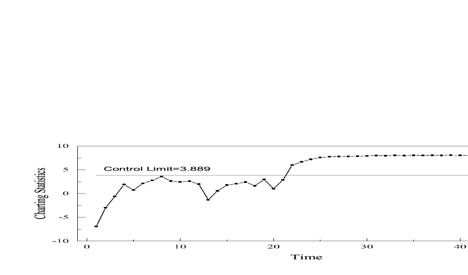
Figure 1: $T_{k}$ statistics (taking logarithms) for monitoring the semiconductor manufacturing process

To demonstrate the implementation of our proposed $T_{k}$ statistic, we first transform the original continuous observations into categorical data. Specifically, we regard all the 1,463 conforming vectors of dimension $461$ as the historical IC dataset and take the averages of each variable as the thresholds that classify the continuous values into two attribute levels. Consequentially, this leads to 461 categorical data streams all with two levels, and we obtain the IC probabilities of each CDS.

In Phase II, the sample size $N$ is set as four. Here we monitor the remaining 104 nonconforming observations together with 80 conforming observations. Note that they have all been dichotomized by the thresholds calculated based on the IC dataset. In addition, we set the IC ARL as 500 with the corresponding control limit 3.889 (after taking the natural logarithm). The $T_{k}$ statistics are calculated based on equation (7) and the above $20+26=46$ samples. After the logarithm operation, they are plotted in Figure 1. According to it, this chart signals an OC alarm at the 22nd sample and remains above the control limit.

6 Conclusion

In this article, we propose a powerful statistic $T_{k}$ to globally monitor a large number of categorical data streams, including nominal ones with several attribute levels and ordinal ones with some natural order among their attribute levels. Our proposed method first eliminates the heterogeneity brought by different nature and parameters of the data streams, and naturally integrates the local information from each data stream based on a powerful goodness-of-fit test. Compared with two other existing global monitoring approaches, numerical simulations reveal that the proposed statistic is either the best or very close to the best in detecting changes in the probability vectors of nominal CDSs or latent location shifts of ordinal CDSs.

Although our proposed monitoring statistic is sensitive to various changes in each CDS, diagnosing OC data streams and identifying root causes remain an open problem. Moreover, here we assume that all CDSs shift at the same time, which is not always the case in practice. After relaxing this assumption, how to efficiently monitor a large number of categorical data streams simultaneously with multiple change-points also requires future research.

References

Bersimis, S., Psarakis, S., and Panaretos, J. (2007). Multivariate statistical process control charts: an overview. Quality and Reliability Engineering International, 23(5), 517–543.

Capizzi G., and Masarotto G. (2011). A Least Angle Regression Control Chart for Multidimensional Data. Technometrics, 53(3), 285–296.

Chiu, J., and Kuo, T. (2008). Attribute control chart for multivariate Poisson distribution. Communications in Statistics: Theory and Methods, 37(1), 146–158.

He, S., He, Z., and Wang, G. (2014). CUSUM Control Charts for Multivariate Poisson Distribution. Communications in Statistics, 43(6), 1192–1208.

Kamranrad, R., Amiri, A., and Niaki, S. T. A. (2017). New approaches in monitoring multivariate categorical processes based on contingency tables in phase II. Quality and Reliability Engineering International, 33(5), 1105–1129.

Li, J., Tsung, F., and Zou, C. (2012). Directional Control Schemes for Multivariate Categorical Processes. Journal of Quality Technology, 44(2), 136–154.

Li, J., Tsung, F., and Zou, C. (2014a). Multivariate binomial/multinomial control chart, IIE Transactions, 46(5), 526–542.

Li J., Tsung, F., and Zou, C. (2014b). A simple categorical chart for detecting location shifts with ordinal information, International Journal of Production Research, 52(2), 550–562.

Li, J., Xu, J., and Zhou, Q. (2018). Monitoring serially dependent categorical processes with ordinal information. IISE Transaction, 50(12), 596–605.

Liu, K., Mei, Y., and Shi, J. (2015). An adaptive sampling strategy for online high-dimensional process monitoring. Technometrics, 57(3), 305–319.

Lu, X.S., Xie, M., Goh, T.N., and Lai, C.D. (1998). Control charts for multivariate attribute processes. International Journal of Production Research, 36(12), 3477–3489.

Lowry, C.A., and Montgomery, D.C. (1995). A review of multivariate control charts. IIE Transactions, 27(6), 800–810.

Marcucci, M. (1985). Monitoring multinomial processes. Journal of Quality Technology, 17(2), 86–91.

Mei, Y. (2010). Efficient scalable schemes for monitoring a large number of data streams. Biometrika, 97(2), 419–433.

Patel, H.I. (1973). Quality control methods for multivariate binomial and Poisson distributions. Technometrics, 15(1), 103–112.

Tartakovsky, A. G., Rozovskii, B. L., Blazek, R. B., and Kim, H. (2006). Detection of intrusions in information systems by sequential change-point methods. Statistical Methodology, 3(3), 252–293.

Woodall, W. H. (1997). Control charts based on attribute data: bibliography and review. Journal of Quality Technology, 29(2), 172–183.

Wang, Z., Li, Y., and Zhou, X. (2017). A Statistical Control Chart for Monitoring High-dimensional Poisson Data Streams. Quality and Reliability Engineering International, 33(2), 307–321.

Wang, K., and Jiang, W. (2009). High-Dimensional Process Monitoring and Fault Isolation via Variable Selection. Journal of Quality Technology, 41(3), 247–258.

Zhang, J. (2002). Powerful goodness-of-fit tests based on the likelihood ratio. Journal of the Royal Statistical Society, series B, 64(2), 281–294.

Zou, C., and Qiu, P. (2009). Multivariate Statistical Process Control Using LASSO. Publications of the American Statistical Association, 104(488), 1586–1596.

Zou, C., Wang, Z., Zi, X., and Jiang, W. (2015). An efficient online monitoring method for high-dimensional data streams. Technometrics, 57(3), 374–387.