Hierarchical Clustering:
$O(1)$-Approximation for Well-Clustered Graphs

Abstract

Hierarchical clustering studies a recursive partition of a data set into clusters of successively smaller size, and is a fundamental problem in data analysis. In this work we study the cost function for hierarchical clustering introduced by Dasgupta [Das16], and present two polynomial-time approximation algorithms: Our first result is an $O(1)$-approximation algorithm for graphs of high conductance. Our simple construction bypasses complicated recursive routines of finding sparse cuts known in the literature (e.g., [CAKMTM19, CC17]). Our second and main result is an $O(1)$-approximation algorithm for a wide family of graphs that exhibit a well-defined structure of clusters. This result generalises the previous state-of-the-art [CAKMT17], which holds only for graphs generated from stochastic models. The significance of our work is demonstrated by the empirical analysis on both synthetic and real-world data sets, on which our presented algorithm outperforms the previously proposed algorithm for graphs with a well-defined cluster structure [CAKMT17].

1 Introduction

Hierarchical clustering (HC) studies a recursive partition of a data set into clusters of successively smaller size, via an effective binary tree representation. As a basic technique, hierarchical clustering has been employed as a standard package in data analysis, and has comprehensive applications in practice. While traditionally HC trees are constructed through bottom-up (agglomerative) heuristics, which lacked a clearly-defined objective function, Dasgupta [Das16] has recently introduced a simple objective function to measure the quality of a particular hierarchical clustering and his work has inspired a number of research on this topic [AAV20, CAKMT17, CAKMTM19, CC17, CCN19, CCNY19, MW17, RP17]. Consequently, there has been a significant interest in studying efficient HC algorithms that not only work in practice, but also have proven theoretical guarantees with respect to Dasgupta’s cost function.

1.1 Our contribution

We present two new approximation algorithms for constructing HC trees that can be rigorously analysed with respect to Dasgupta’s cost function. For our first result, we construct an HC tree of an input graph $G$ entirely based on the degree sequence of $V(G)$, and show that the approximation guarantee of our constructed tree is with respect to the conductance of $G$, which will be defined formally in Section 2. The striking fact of this result is that, for any $n$-vertex graph $G$ with $m$ edges and conductance $\Omega(1)$ (a.k.a. expander graph), an $O(1)$-approximate HC tree of $G$ can be very easily constructed in $O(m+n\log n)$ time, although obtaining such result for general graphs in polynomial time is impossible under the Small Set Expansion Hypothesis (SSEH) [CC17]. Our theorem is in line with a sequence of results for problems that are naturally linked to the Unique Games and Small Set Expansion problems: it has been shown that such problems are much easier to solve once the input instance exhibits the high conductance property [ABS15, AKK⁺08, Kol10, LSZ19]. However, to the best of our knowledge, our result is the first of this type for hierarchical clustering, and can be informally described as follows:

Theorem 1 (informal statement of Theorem 3).

Given any graph $G=(V,E,w)$ with constant conductance as input, there is an algorithm that runs in $O(|E|+|V|\log(|V|))$ time and returns an $O(1)$-approximate HC tree of $G$.

While our first result presents an interesting theoretical fact, we further study whether we can extend this $O(1)$-approximate construction to a much wider family of graphs occurring in practice. Specifically, we look at well-clustered graphs, i.e., the graphs in which vertices within each cluster are better connected than vertices between different clusters and the total number of clusters is constant. This includes a wide range of graphs occurring in practice with a clear cluster-structure, and have been extensively studied over the past two decades (e.g., [GT14, KVV04, PSZ17, SZ19, vL07]). As our second and main result, we present an approximation algorithm for well-clustered graphs, and our result is informally described as follows:

Theorem 2 (informal statement of Theorem 4).

Let $G=(V,E,w)$ be a well-clustered graph with $O(1)$ clusters. Then, there is a polynomial-time algorithm that constructs an $O(1)$-approximate HC tree of $G$.

Given that the class of well-clustered graphs includes graphs with clusters of different sizes and asymmetrical internal structure, our result significantly improves the previous state-of-the-art [CAKMT17], which only holds for graphs generated from stochastic models. At the technical level, the design of our algorithm is based on the graph decomposition algorithm presented in [GT14], which is designed to find a good partition of a well-clustered graph. However, our analysis suggests that, in order to obtain an $O(1)$-approximation algorithm, directly applying their decomposition is not sufficient for our purpose. To overcome this bottleneck, we refine their output decomposition via a pruning technique, and carefully merge the refined parts to construct our final HC tree. In our point of view, our presented stronger graph decomposition procedure might have applications in other settings as well.

To demonstrate the significance of our work, we compare our algorithm against the previous state-of-the-art with similar approximation guarantee [CAKMT17] and well-known linkage heuristics on both synthetic and real-world data sets. Although our algorithm’s performance is marginally better than [CAKMT17] for the graphs generated from the stochastic block models (SBM), the cost of our algorithm’s output is up to $50\%$ lower than the one from [CAKMT17] when the clusters of the input graph have different sizes and some cliques are embedded into a cluster.

1.2 Related work

Our work fits in a line of research initiated by Dasgupta [Das16], who introduced a cost function to measure the quality of an HC tree. Dasgupta proved that a recursive application of the algorithm for the Sparsest Cut problem can be used to construct an $O(\log^{3/2}n)$-approximate HC tree. The approximation factor was first improved to $O(\log n)$ by Roy and Pokutta [RP17]. Charikar and Chatziafratis [CC17] improved Dasgupta’s analysis of the recursive sparsest cut algorithm by establishing the following black-box connection: an $\alpha$-approximate algorithm for the Sparsest Cut problem can be used to construct an $O(\alpha)$-approximate HC tree according to Dasgupta’s cost function. Hence, an $O(\sqrt{\log n})$-approximate HC tree can be computed in polynomial time by using the celebrated result of [ARV09]. For general input instances, it is known to be NP-hard to find an optimal HC tree [Das16], and SSEH-hard to achieve an $O(1)$-approximation with respect to Dasgupta’s cost function [RP17, CC17].

Cohen-Addad et al. [CAKMTM19] analysed the performance of several linkage heuristics (e.g., Average Linkage) for constructing HC trees, and showed that such algorithms could output an HC tree of high cost in the worst case. Moving beyond the worst-case scenario, Cohen-Addad et al. [CAKMT17] studied a hierarchical extension of the SBM and showed that, for graphs generated according to this model, a certain SVD projection algorithm [McS01] together with several linkage heuristics can be applied to construct a $(1+o(1))$-approximate HC tree with high probability. We emphasise that our notion of well-clustered graphs generalises the SBM variant studied in [CAKMT17], and does not assume the rigid hierarchical structure of the clusters.

For another line of related work, Moseley and Wang [MW17] studied the dual objective function and proved that Average Linkage achieves a $(1/3)$-approximation for the new objective. Notice that, although this has received significant attention very recently [AAV20, CCN19, CCNY19, CYL⁺20, VCC⁺21], achieving an $O(1)$-approximation is tractable under this alternative objective. This suggests the fundamental difference on the hardness of the problem under different objective functions, and is our reason to entirely focus on Dasgupta’s cost function in this work.

1.3 Organisation

The remaining part of the paper is organised as follows: we introduce the necessary notation about graphs and matrices, the basis of hierarchical clustering and graph partitioning in Section 2. In Section 3, we present and analyse the algorithm of constructing an HC tree for graphs of high conductance. We present and analyse our main algorithm, i.e., the algorithm for constructing $O(1)$-approximate HC trees for well-clustered graphs in Section 4. In Section 5 we present the experimental analysis where we compared our developed algorithm against other algorithms in the literature. We end the paper with several concluding remarks and directions of future work in Section 6.

2 Preliminaries

Throughout the paper, we always assume that $G=(V,E,w)$ is an undirected graph with $|V|=n$ vertices, $|E|=m$ edges and weight function $w:V\times V\rightarrow\mathbb{R}_{\geq 0}$. For any edge $e=\{u,v\}\in E$, we write $w_{e}$ or $w_{uv}$ to indicate the similarity weight between $u$ and $v$. For a vertex $u\in V$, we denote its degree by $d_{u}\triangleq\sum_{v\in V}w_{uv}$ and we assume that $w_{\mathrm{max}}/w_{\mathrm{min}}=O(\mathrm{poly}(n))$, where $w_{\mathrm{min}}(w_{\mathrm{max}})$ is the minimum (maximum) edge weight. We will use $d_{\min},d_{\max}$, and $d_{\mathrm{avg}}$ for the minimum, maximum and average degrees in $G$ respectively, where $d_{\mathrm{avg}}\triangleq\sum_{u\in V}d_{u}/n$. For a nonempty subset $S\subset V$, we define $G[S]$ to be the induced subgraph on $S$ and we denote by $G\{S\}$ the subgraph $G[S]$, where self loops are added to vertices $v\in S$ such that their degrees in $G$ and $G\{S\}$ are the same. For any two subsets $S,T\subset V$, we define the cut value $w(S,T)\triangleq\sum_{e\in E(S,T)}w_{e}$, where $E(S,T)$ is the set of edges between $S$ and $T$. For any $G=(V,E,w)$ and set $S\subseteq V$, the volume of $S$ is $\mathrm{vol}_{G}(S)\triangleq\sum_{u\in S}d_{u}$, and we write $\mathrm{vol}(G)$ when referring to $\mathrm{vol}_{G}(V)$. Sometimes we drop the subscript $G$ when it is clear from the context. For any nonempty subset $S\subseteq V$, we define the conductance of $S$ by

$$\Phi_{G}(S)\triangleq\frac{w(S,V\setminus S)}{\mathrm{vol}(S)}.$$

Notice that $\Phi_{G}(V)=0$ and we conventionally choose $\Phi_{G}(\emptyset)=1$, where $\emptyset$ is the empty set. Furthermore, we define the conductance of the graph $G$ by

$$\Phi_{G}\triangleq\min_{\begin{subarray}{c}S\subset V\\ \mathrm{vol}(S)\leq\mathrm{vol}(V)/2\end{subarray}}\Phi_{G}(S),$$

and we call $G$ an expander graph if $\Phi_{G}=\Omega(1)$.

For a graph $G=(V,E,w)$, let $\mathbf{D}\in\mathbb{R}^{n\times n}$ be the diagonal matrix defined by $\mathbf{D}_{uu}=d_{u}$ for all $u\in V$. We denote by $\mathbf{A}\in\mathbb{R}^{n\times n}$ the adjacency matrix of $G$, where $\mathbf{A}_{uv}=w_{uv}$ for all $u,v\in V$. The normalised Laplacian matrix of $G$ is defined as $\mathbf{\mathcal{L}}\triangleq\mathbf{I}-\mathbf{D}^{-1/2}\mathbf{A}\mathbf{D}^{-1/2}$, where $\mathbf{I}$ is the $n\times n$ identity matrix. The normalised Laplacian $\mathbf{\mathcal{L}}$ is symmetric and real-valued, therefore it has $n$ real eigenvalues which we will write as $\lambda_{1}\leq\ldots\leq\lambda_{n}$. It is known that $\lambda_{1}=0$ and $\lambda_{n}\leq 2$ [Chu97].

2.1 Hierarchical clustering

A hierarchical clustering (HC) tree of a given graph $G$ is a binary tree $\mathcal{T}$ with $n$ leaf nodes such that each leaf corresponds to exactly one vertex $v\in V(G)$. Let $\mathcal{T}$ be an HC tree of some graph $G=(V,E,w)$, and $N\in\mathcal{T}$ be an arbitrary internal node of $\mathcal{T}$. We write $N\rightarrow(N_{1},N_{2})$ to indicate that $N_{1}$ and $N_{2}$ are the children of $N$. We denote $\mathcal{T}[N]$ to be the subtree of $\mathcal{T}$ rooted at $N$, $\mathsf{leaves}\left(\mathcal{T}[N]\right)$ to be the set of leaf nodes of $\mathcal{T}[N]$ and $\mathrm{parent}_{\mathcal{T}}(N)$ to be the parent of node $N$ in $\mathcal{T}$. In addition, each internal node $N\in\mathcal{T}$ induces a unique vertex set $C\subseteq V$ formed by the vertices corresponding to $\mathsf{leaves}(\mathcal{T}[N])$. For the ease of presentation, we will sometimes abuse the notation, and write $N\in\mathcal{T}$ for both the internal node of $\mathcal{T}$ and the corresponding subset of vertices in $V$.

To measure the quality of an HC tree $\mathcal{T}$ with similarity weights, Dasgupta [Das16] introduced the cost function defined by

$$\mathrm{cost}_{G}(\mathcal{T})\triangleq\sum_{e=\{u,v\}\in E}w_{e}\cdot\lvert\mathsf{leaves}\left(\mathcal{T}[u\vee v]\right)\rvert,$$

where $u\vee v$ is the lowest common ancestor of $u$ and $v$ in $\mathcal{T}$. Trees that achieve a better hierarchical clustering have a lower cost, and the objective of HC is to construct trees with the minimum cost based on the following consideration: for any pair of vertices $u,v\in V$ that corresponds to an edge of high weight $w_{uv}$ (i.e., $u$ and $v$ are highly similar) a “good” HC tree would separate $u$ and $v$ lower in the tree, thus reflected in a small size $|\mathsf{leaves}(\mathcal{T}[u\vee v])|$. We denote by $\mathsf{OPT}_{G}$ the minimum cost of any HC tree of $G$, i.e., $\mathsf{OPT}_{G}=\min_{\mathcal{T}}\mathrm{cost}_{G}(\mathcal{T})$, and use the notation $\mathcal{T}^{*}$ to refer to an optimal tree achieving the minimum cost. We say that an HC tree $\mathcal{T}$ is an $\alpha$-approximate tree if $\mathrm{cost}_{G}(\mathcal{T})\leq\alpha\cdot\mathsf{OPT}_{G}$, for some $\alpha\geq 1$.

Sometimes, it is convenient to consider the cost of an edge $e=\{u,v\}\in E$ in $\mathcal{T}$ as

$$\mathrm{cost}_{\mathcal{T}}(e)\triangleq w_{e}\cdot\lvert\mathsf{leaves}(\mathcal{T}[u\vee v])\rvert,$$

so that we can write

$$\mathrm{cost}_{G}(\mathcal{T})=\sum_{e\in E}\mathrm{cost}_{\mathcal{T}}(e).$$

Alternatively, as observed by Dasgupta [Das16], the cost function can be expressed with respect to all cut values induced at every internal node.

Lemma 2.1 ([Das16]).

The cost function of an HC tree $\mathcal{T}$ of $G$ can be written as

$$\mathrm{cost}_{G}(\mathcal{T})=\sum_{\begin{subarray}{c}N\in\mathcal{T}\\ N\rightarrow(N_{1},N_{2})\end{subarray}}\lvert\mathsf{leaves}(\mathcal{T}[N])\rvert\cdot w(\mathsf{leaves}(\mathcal{T}[N_{1}]),\mathsf{leaves}(\mathcal{T}[N_{2}])),$$

where the sum is taken over all internal nodes $N$.

The following lemma presents a simple upper bound on the cost of any HC tree $\mathcal{T}$:

Lemma 2.2.

It holds for any HC tree $\mathcal{T}$ of $G$ that

$$\mathrm{cost}_{G}(\mathcal{T})\leq\frac{n\cdot\mathrm{vol}(G)}{2}.$$

Proof.

For any HC tree $\mathcal{T}$ of $G$, we have that

$$\mathrm{cost}_{G}(\mathcal{T})=\sum_{e\in E}\mathrm{cost}_{\mathcal{T}}(e)\leq\sum_{e\in E}n\cdot w_{e}\leq\frac{n\cdot\mathrm{vol}(G)}{2},$$

which proves the statement. ∎

2.2 Graph partitioning

The following results on graph partitioning will be used in our analysis, and we list them here for completeness.

Lemma 2.3 (Cheeger Inequality, [Alo86]).

It holds for any graph $G$ that

$$\frac{\lambda_{2}}{2}\leq\Phi_{G}\leq\sqrt{2\lambda_{2}}.$$

Furthermore, there is a nearly-linear time algorithm (i.e., the Spectral Partitioning algorithm) that finds a set $S$ such that $\mathrm{vol}(S)\leq\mathrm{vol}(V)/2$, and $\Phi_{G}(S)\leq 2\cdot\sqrt{\Phi_{G}}$.

One can generalise the notion of conductance, and for any $k\geq 2$ define the $k$-way expansion of $G$ by

$$\rho(k)\triangleq\min_{\mathrm{disjoint\>}S_{1},\dots,S_{k}}\max_{1\leq i\leq k}\Phi_{G}(S_{i}).$$

Lemma 2.4 (Higher-Order Cheeger Inequality, [LGT14]).

It holds for any graph $G$ and $k\geq 2$ that

$$\frac{\lambda_{k}}{2}\leq\rho(k)\leq O(k^{2})\sqrt{\lambda_{k}}.$$

Lemma 2.5 (Lemma 1.13, [GT14]).

There is a universal constant $c_{0}>1$ such that for any $k\geq 2$ and any partitioning of $V$ into $r$ sets $P_{1},\dots P_{r}$ of $V$, where $r\leq k-1$, we have that

$$\min_{1\leq i\leq r}\lambda_{2}(G[P_{i}])\leq 2c_{0}\cdot k^{6}\cdot\lambda_{k}.$$

3 Hierarchical clustering for graphs of high conductance

In this section we study hierarchical clustering for graphs with high conductance and prove that, for any input graph $G$ with $\Phi_{G}=\Omega(1)$, an $O(1)$-approximate HC tree of $G$ can be simply constructed based on the degree sequence of $G$. This section is organised as follows: in Section 3.1, we give an upper bound for the cost of any HC tree $\mathcal{T}$ based on the degree distribution and conductance of $G$. In Section 3.2, we present an algorithm for constructing an HC tree for graphs of high conductance, whose analysis is presented in Section 3.3.

3.1 Upper bounding $\mathrm{cost}_{G}(\mathcal{T})$ with respect to the degrees of $G$

As a starting point, we show that $\mathrm{cost}_{G}(\mathcal{T})$ for any $\mathcal{T}$ can be upper bounded with respect to $\Phi_{G}$ and the degree distribution of $V(G)$.

Lemma 3.1.

It holds for any HC tree $\mathcal{T}$ of graph $G$ that $\mathrm{cost}_{G}(\mathcal{T})\leq\frac{9}{4\Phi_{G}}\cdot\min\left\{\frac{d_{\mathrm{avg}}}{d_{\min}},\frac{d_{\max}}{d_{\mathrm{avg}}}\right\}\cdot\mathsf{OPT}_{G}.$

The proof is based on a combination of Lemma 2.2 and the following technical result:

Lemma 3.2.

It holds for any optimal HC tree $\mathcal{T}^{*}$ of graph $G$ that

$$\mathrm{cost}_{G}(\mathcal{T}^{*})\geq\frac{2\Phi_{G}}{9}\cdot\max\left\{\frac{\mathrm{vol}(G)^{2}}{d_{\max}},d_{\min}\cdot n^{2}\right\}=\frac{2\Phi_{G}}{9}\cdot n\cdot\mathrm{vol}(G)\cdot\max\left\{\frac{d_{\mathrm{avg}}}{d_{\max}},\frac{d_{\min}}{d_{\mathrm{avg}}}\right\}.$$

We remark that, as a corollary, the lower bound above holds for any HC tree $\mathcal{T}$ of $G$.

Proof of Lemma 3.2.

We will give two lower bounds for $\mathrm{cost}_{G}(\mathcal{T}^{*})$. Let $A_{0}$ be the root of $\mathcal{T}^{*}$. For the first lower bound, we start with the root node $A_{0}$ and travel along $\mathcal{T}^{*}$ recursively as follows: at every intermediate node $A_{i}$, we travel down to the node of higher volume among its two children. This process stops when we reach node $A_{k}$ such that $\mathrm{vol}(A_{k})\leq\frac{2\mathrm{vol}(G)}{3}$. We denote $\left(A_{0},\dots,A_{k}\right)$ to be the path in $\mathcal{T}^{*}$ from the root $A_{0}$ to $A_{k}$ and we define $A\triangleq A_{k}$ as well as $B\triangleq V\setminus A_{k}$. By construction, it holds that $\mathrm{vol}(A)>\mathrm{vol}(G)/3$ and $\mathrm{vol}(B)\geq\mathrm{vol}(G)/3$. We will show that the cut $(A,B)$ has significant contribution to $\mathrm{cost}_{G}\left(\mathcal{T}^{*}\right)$.

By the stopping criteria, we know that $\mathrm{vol}(A_{i})>\frac{2\mathrm{vol}(G)}{3}$ for every $0\leq i<k$. For any edge $e=\{u,v\}$ in the cut $(A,B)$, if $A_{i}=u\vee v$ for some $0\leq i<k$, then we have that

$$\lvert\mathsf{leaves}\left(\mathcal{T}^{*}[u\vee v]\right)\rvert=|A_{i}|=\frac{\mathrm{vol}(A_{i})}{d_{\mathrm{avg}}(A_{i})}>\frac{2\cdot\mathrm{vol}(G)}{3\cdot d_{\mathrm{max}}}.$$

Therefore, we have that

$$\mathrm{cost}_{G}(\mathcal{T}^{*}) =\sum_{e=\{u,v\}}w_{e}\cdot\lvert\mathsf{leaves}\left(\mathcal{T}^{*}[u\vee v]\right)\rvert\geq\sum_{\begin{subarray}{c}e\in E(A,B)\\ e=\{u,v\}\end{subarray}}w_{e}\cdot\lvert\mathsf{leaves}\left(\mathcal{T}^{*}[u\vee v]\right)\rvert$$

$$\geq\frac{2}{3}\cdot\frac{\mathrm{vol}(G)}{d_{\mathrm{max}}}\cdot w(A,B)\geq\frac{2}{3}\cdot\frac{\mathrm{vol}(G)}{d_{\mathrm{max}}}\cdot\Phi_{G}\cdot\min\{\mathrm{vol}(A),\mathrm{vol}(B)\}$$

$$\geq\frac{2}{3}\cdot\frac{\mathrm{vol}(G)}{d_{\mathrm{max}}}\cdot\Phi_{G}\cdot\frac{\mathrm{vol}(G)}{3}$$

$$=\frac{2\Phi_{G}\cdot\mathrm{vol}(G)^{2}}{9\cdot d_{\mathrm{max}}}.$$

The second lower bound is proven in a similar way: we start with the root node $A_{0}$, and travel along $\mathcal{T}^{*}$ recursively as follows: at every intermediate node $A_{i}^{\prime}$ we travel down to the node of larger size; this process stops when we reach node $A^{\prime}_{\ell}$ such that $|A^{{}^{\prime}}_{\ell}|\leq 2n/3$. We denote $(A_{0}=A_{0}^{\prime},\ldots,A^{{}^{\prime}}_{\ell})$ to be the path in $\mathcal{T}^{*}$ from the root to $A_{\ell}^{\prime}$, and we define $A^{{}^{\prime}}\triangleq A^{{}^{\prime}}_{\ell}$ as well as $B^{{}^{\prime}}\triangleq V\setminus A^{{}^{\prime}}_{\ell}$. By construction, it holds that $|A^{{}^{\prime}}|>n/3$, and $|B^{{}^{\prime}}|>n/3$. We will show that the cut $(A^{{}^{\prime}},B^{{}^{\prime}})$ has significant contribution to $\mathrm{cost}_{G}(\mathcal{T}^{*})$.

Similar to the analysis in the first case, by the stopping criteria we have that $|A^{\prime}_{i}|>\frac{2n}{3}$, for all $0\leq i<\ell$. Moreover, for any $e=(u,v)\in E(A^{\prime},B^{\prime})$, we have that $|\mathsf{leaves}(\mathcal{T}^{*}[u\vee v])|>\frac{2n}{3}$. Hence, it holds that

$$\mathrm{cost}_{G}(\mathcal{T}^{*}) =\sum_{e=\{u,v\}}w_{e}\cdot\lvert\mathsf{leaves}\left(\mathcal{T}^{*}[u\vee v]\right)\rvert\geq\sum_{e=\{u,v\}\in E(A^{\prime},B^{\prime})}w_{e}\cdot\lvert\mathsf{leaves}\left(\mathcal{T}^{*}[u\vee v]\right)\rvert$$

$$\geq\frac{2n}{3}\cdot w(A,B)\geq\frac{2n}{3}\cdot\Phi_{G}\cdot\min\{\mathrm{vol}(A),\mathrm{vol}(B)\}$$

$$\geq\frac{2n}{3}\cdot\Phi_{G}\cdot d_{\min}\cdot\frac{n}{3}$$

$$=\frac{2\Phi_{G}\cdot n^{2}\cdot d_{\min}}{9}.$$

Combining the two cases above gives us that

$$\mathrm{cost}_{G}(\mathcal{T}^{*})\geq\frac{2\Phi_{G}}{9}\cdot\max\left\{\frac{\mathrm{vol}(G)^{2}}{d_{\max}},d_{\min}\cdot n^{2}\right\},$$

which proves the statement. ∎

Proof of Lemma 3.1.

Let $\mathcal{T}$ be an arbitrary HC tree, and $\mathcal{T}^{*}$ be an optimal tree. Combining Lemmas 2.2 and 3.2, we have that

$$\frac{\mathrm{cost}_{G}(\mathcal{T})}{\mathrm{cost}_{G}(\mathcal{T}^{*})} \leq\frac{n\cdot\mathrm{vol}(G)}{2}\cdot\frac{9}{2\Phi_{G}\cdot n\cdot\mathrm{vol}(G)\cdot\max\left\{\frac{d_{\mathrm{avg}}}{d_{\max}},\frac{d_{\min}}{d_{\mathrm{avg}}}\right\}}$$

$$=\frac{9}{4\cdot\Phi_{G}}\cdot\min\left\{\frac{d_{\mathrm{avg}}}{d_{\min}},\frac{d_{\max}}{d_{\mathrm{avg}}}\right\},$$

which proves the statement. ∎

3.2 The algorithm for graphs of high conductance

While Lemma 3.1 holds for any graph $G$, it implies some interesting facts for expander graphs: first of all, when $G=(V,E,w)$ satisfies $d_{\max}/d_{\min}=O(1)$ and $\Phi_{G}=\Omega(1)$, Lemma 3.1 shows that any HC tree $\mathcal{T}$ is an $O(1)$-approximate tree. In addition, although $\Phi_{G}$ plays a crucial role in analysing $\mathrm{cost}_{G}(\mathcal{T})$ as for many other graph problems, Lemma 3.1 indicates that the degree distribution of $G$ might also have a significant impact. One could naturally ask the extend to which the degree distribution of $V(G)$ would influence the construction of $\mathsf{OPT}_{G}$. To answer this question, we study the following example.

Example 3.3.

We study the following graph $G$, in which all the edges have unit weight:

1. Let $G_{1}=(V,E_{1})$ be a constant-degree expander graph of $n$ vertices with $\Phi_{G_{1}}=\Omega(1)$, e.g., the ones presented in [HLW06];

2. We choose $\lfloor n^{2/3}\rfloor$ vertices from $V$ to form $S$, and let $K=(S,S\times S)$ be a complete graph defined on $S$;

3. Partition the vertices of $V\setminus S$ into $\lfloor n^{2/3}\rfloor$ groups of roughly the same size, associate each group to a unique vertex in $S$, and let $E_{2}$ be the set of edges formed by connecting every vertex in $S$ with all the vertices in its associated group;

4. We define $G\triangleq(V,E_{1}\cup(S\times S)\cup E_{2})$, see Figure 1(a) for illustration.

By construction, we know that $\Phi_{G}=\Omega(1)$, and the degrees of $G$ satisfy $d_{\max}=\Theta(n^{2/3})$, $d_{\min}=\Theta(1)$, and $d_{\mathrm{avg}}=\Theta(n^{1/3})$ as $\mathrm{vol}(G)=\Theta(n^{4/3})$. Therefore, the ratio between $\mathrm{cost}_{G}(\mathcal{T})$ for any HC tree $\mathcal{T}$ and $\mathsf{OPT}_{G}$ could be as high as $\Theta(n^{1/3})$. On the other side, it is not difficult to show that the tree $\mathcal{T}^{*}$ illustrated in Figure 1(b), which first separates the set $S$ of high-degree vertices from $V\setminus S$ at the top of the tree, actually $O(1)$-approximates $\mathsf{OPT}_{G}$. To see this, notice that $\mathrm{cost}(\mathcal{T}^{*})~{}\leq~{}\mathrm{cost}(\mathcal{\mathcal{T}^{*}}[S])+n\cdot\mathrm{vol}(G_{1})+n^{2}=\Theta(n^{2})$, as the complete subgraph $G[S]$ induces a cost of $\Theta((n^{2/3})^{3})$ [Das16]. The existence of the subgraph $G[S]$ also implies that $\mathsf{OPT}_{G}=\Omega(n^{2})$.

(a)

(b)

Figure 1: (a) Our constructed graph $G$; (b) the tree that separates the vertices of high degrees from the others achieves $O(1)$-approximation.

This example suggests that grouping vertices of similar degrees first would potentially help reduce $\mathrm{cost}_{G}(\mathcal{T})$ for our constructed $\mathcal{T}$. This motivates us to design the following Algorithm 1 to construct an HC tree, and the algorithm’s performance is summarised in Theorem 3. We highlight that the output of Algorithm 1 is uniquely determined by the ordering of the vertices of $G$ according to their degrees, which can be computed in $O\left(n\cdot\log n\right)$ time.

Input: $G=(V,E,w)$ with the ordered vertices such that $d_{v_{1}}\geq\ldots\geq d_{v_{|V|}}$;

Output: An HC tree $\mathcal{T}_{\deg}(G)$;

1 if $|V|=1$ then

2       return the single vertex in $V$ as the tree;

3else

4       $i_{\max}:=\lfloor\log_{2}(|V|-1)\rfloor$; $r:=2^{i_{\max}}$; $A:=\left\{v_{1},\ldots,v_{r}\right\}$; $B:=V\setminus A$;

5      Let $\mathcal{T}_{1}:=\mathrm{\texttt{HCwithDegrees}}(G\{A\});\mathcal{T}_{2}:=\mathrm{\texttt{HCwithDegrees}}(G\{B\})$;

6      return $\mathcal{T}_{\deg}$ with $\mathcal{T}_{1}$ and $\mathcal{T}_{2}$ as the two children.

Algorithm 1 HCwithDegrees$(G\{V\})$

Theorem 3.

Given any graph $G=(V,E,w)$ with conductance $\Phi_{G}$ as input, Algorithm 1 runs in $O(m+n\log n)$ time, and returns an HC tree $\mathcal{T}_{\deg}$ of $G$ that satisfies $\mathrm{cost}_{G}(\mathcal{T}_{\deg})=O\left(1/\Phi_{G}^{4}\right)\cdot\mathsf{OPT}_{G}$.

Theorem 3 shows that, when the input $G$ satisfies $\Phi_{G}=\Omega(1)$, the output $\mathcal{T}_{\deg}$ of Algorithm 1 achieves an $O(1)$-approximation. It is important to notice that, while it is known [CC17] that there is no polynomial-time algorithm that $O(1)$-approximates $\mathsf{OPT}_{G}$ for a general graph $G$ under the SSEH, our result shows that an $O(1)$-approximate HC tree can be constructed in polynomial-time for expander graphs. Our result is in line with a sequence of research showing that this type of problems become easier when the input graphs exhibit a good expansion property (e.g., [ABS15, AKK⁺08, Kol10, LSZ19]). To the best of our knowledge, Theorem 3 is the first such result for hierarchical clustering on graphs of high expansion conductance. Moreover, as the high-conductance property can be determined in nearly-linear time by computing $\lambda_{2}(\mathcal{L}_{G})$ and applying the Cheeger inequality, Algorithm 1 presents a very simple construction of an $O(1)$-approximate HC tree once the input $G$ is known to have high conductance.

3.3 Analysis of the algorithm

In this subsection we analyse Algorithm 1, and prove Theorem 3.

3.3.1 The dense branch and its properties

Our analysis is crucially based on the notion of dense branch, which can be informally described as follows: for any given $\mathcal{T}$, we perform a traversal in $\mathcal{T}$ starting at its root node $A_{0}$ and sequentially travel to the child of higher volume. The process stops whenever we reach a node $A_{k}$, for some $k\in\mathbb{Z}_{\geq 0}$, such that $\mathrm{vol}(A_{k})>\mathrm{vol}(G)/2$ and both of its children have volume at most $\mathrm{vol}(G)/2$. The sequence of visited nodes in this process is the dense branch of $\mathcal{T}$. Formally, we define the dense branch as follows:

Definition 3.4 (Dense branch).

Given a graph $G$ with an HC tree $\mathcal{T}$, the dense branch is the path $(A_{0},A_{1},\dots,A_{k})$ in $\mathcal{T}$, for some $k\in\mathbb{Z}_{\geq 0}$, such that the following hold:

1. $A_{0}$ is the root of $\mathcal{T}$;

2. $A_{k}$ is the node such that $\mathrm{vol}(A_{k})>\mathrm{vol}(G)/2$ and both of its children have volume at most $\mathrm{vol}(G)/2$.

It is important to note that the dense branch of $\mathcal{T}$ is unique, and consists of all the nodes $A_{i}$ with $\mathrm{vol}(A_{i})>\mathrm{vol}(G)/2$. Moreover, for every pair of consecutive nodes $A_{i},A_{i+1}$ on the dense branch, $A_{i+1}$ is the child of $A_{i}$ of the higher volume. Now we will present some properties of the dense branch, which will be used extensively in our analysis.

Lemma 3.5 (Lower bound of $\mathrm{cost}_{G}(\mathcal{T})$ based on the dense branch).

Let $G$ be a graph of conductance $\Phi_{G}$, and let $\mathcal{T}$ be an arbitrary HC tree of $G$. Suppose $(A_{0},\dots,A_{k})$ is the dense branch of $\mathcal{T}$, for some $k\in\mathbb{Z}_{\geq 0}$, and suppose each node $A_{i}$ has sibling $B_{i}$, for all $1\leq i\leq k$. Then, the following lower bounds of $\mathrm{cost}_{G}(\mathcal{T})$ hold:

1. $\mathrm{cost}_{G}(\mathcal{T})\geq\frac{\Phi_{G}}{2}\sum_{i=1}^{k}|A_{i-1}|\cdot\mathrm{vol}(B_{i})$;

2. $\mathrm{cost}_{G}(\mathcal{T})\geq\frac{\Phi_{G}}{2}\cdot|A_{k}|\cdot\mathrm{vol}(A_{k})$.

Proof.

Let $\mathcal{S}=\{A_{k},B_{1},\dots,B_{k}\}$. We focus on the edges $e$ crossing different pairs $(X,Y)$ of $X,Y\in\mathcal{S}$, and have that

$$\mathrm{cost}_{G}(\mathcal{T}) \geq\sum_{\begin{subarray}{c}(X,Y)\in\mathcal{S}^{2}\\ X\neq Y\end{subarray}}\sum_{e\in E(X,Y)}\mathrm{cost}_{\mathcal{T}}(e)=\frac{1}{2}\cdot\sum_{X\in\mathcal{S}}\sum_{e\in E(X,V\setminus X)}\mathrm{cost}_{\mathcal{T}}(e)$$

$$\geq\frac{1}{2}\cdot\sum_{i=1}^{k}\sum_{e\in E(B_{i},V\setminus B_{i})}\mathrm{cost}_{\mathcal{T}}(e)\geq\frac{1}{2}\cdot\sum_{i=1}^{k}\sum_{e\in E(B_{i},V\setminus B_{i})}w_{e}\cdot|A_{i-1}|$$

$$=\frac{1}{2}\cdot\sum_{i=1}^{k}|A_{i-1}|\cdot w(B_{i},V\setminus B_{i})\geq\frac{\Phi_{G}}{2}\cdot\sum_{i=1}^{k}|A_{i-1}|\cdot\mathrm{vol}(B_{i}),$$

where the third inequality holds by the fact that $A_{i-1}$ is the parent of $B_{i}$ and any edge $e$ with exactly one endpoint in $B_{i}$ satisfies $\mathrm{cost}_{\mathcal{T}}(e)\geq w_{e}\cdot|A_{i-1}|$, and the last inequality holds by the fact that $G$ has conductance $\Phi_{G}$ and $\mathrm{vol}(B_{i})\leq\mathrm{vol}(G)/2$ by the definition of the dense branch.

For the second bound, let $A_{k+1},B_{k+1}$ be the children of $A_{k}$ such that $\mathrm{vol}(A_{k+1})\geq\mathrm{vol}(B_{k+1})$. Therefore, we have that

$$\mathrm{cost}_{G}(\mathcal{T}) \geq\sum_{e\in E(A_{k+1},V\setminus A_{k+1})}\mathrm{cost}_{T}(e)\geq\sum_{e\in E(A_{k+1},V\setminus A_{k+1})}w_{e}\cdot|A_{k}|$$

$$\geq|A_{k}|\cdot w(A_{k+1},V\setminus A_{k+1})\geq|A_{k}|\cdot\Phi_{G}\cdot\mathrm{vol}(A_{k+1})$$

$$\geq\frac{\Phi_{G}}{2}\cdot|A_{k}|\cdot\mathrm{vol}(A_{k}).\qed$$

Next, we prove that, if the dense branch of an optimal tree $\mathcal{T}^{*}$ consists of a single node, i.e., the root of $\mathcal{T}^{*}$, then any tree $\mathcal{T}$ achieves a $(1/\Phi_{G})$-approximation. If we assume this corner case occurs, we are able to prove a stronger result over Theorem 3, and this result is presented in the following lemma.

Lemma 3.6.

Let $G$ be a graph of conductance $\Phi_{G}$, and let $\mathcal{T}^{*}$ be any optimal HC tree of $G$ such that its dense branch only consists of the root of $\mathcal{T}^{*}$. Then, it holds for any HC tree $\mathcal{T}$ of $G$ that

$$\mathrm{cost}_{G}(\mathcal{T})\leq\frac{\mathrm{cost}_{G}(\mathcal{T}^{*})}{\Phi_{G}}.$$

In particular, it implies that $\mathrm{cost}_{G}(\mathcal{T}_{\deg})\leq 1/\Phi_{G}\cdot\mathsf{OPT}_{G}$.

Proof.

Suppose the dense branch of $\mathcal{T}^{*}$ only consists of the root node $A_{0}$, and let $A_{1},B_{1}$ be the two children of $A_{0}$ such that $\mathrm{vol}(A_{1})\geq\mathrm{vol}(B_{1})$. Since $A_{1}$ does not belong to the dense branch, we know that $\mathrm{vol}(A_{1})\leq\mathrm{vol}(G)/2$ and hence $\mathrm{vol}(A_{1})=\mathrm{vol}(B_{1})=\mathrm{vol}(G)/2$. Therefore, we have that

$$\mathrm{cost}_{G}(\mathcal{T}^{*})\geq\sum_{e\in E(A_{1},B_{1})}\mathrm{cost}_{\mathcal{T}^{*}}(e)=n\cdot w(A_{1},B_{1})\geq n\cdot\Phi_{G}\cdot\frac{\mathrm{vol}(G)}{2},$$

where the last inequality uses that $G$ has conductance $\Phi_{G}$ and $\mathrm{vol}(A_{1})=\mathrm{vol}(B_{1})=\mathrm{vol}(G)/2$. On the other hand, by Lemma 2.2 it holds for any tree $\mathcal{T}$ that

$$\mathrm{cost}_{G}(\mathcal{T})\leq n\cdot\frac{\mathrm{vol}(G)}{2}.$$

Combining the two inequalities above proves the claimed statement. ∎

Finally, we prove that if the size of the last node on the dense branch of an optimal tree $\mathcal{T}^{*}$ is significantly large, then any tree $\mathcal{T}$ achieves an $O(1/\Phi_{G})$-approximation. Again, if we assume this corner case occurs, we prove a stronger result over Theorem 3 and we present the result in the following lemma.

Lemma 3.7.

Let $G$ be a graph of conductance $\Phi_{G}$, and let $\mathcal{T}^{*}$ be any optimal HC tree of $G$ whose dense branch is $(A_{0},\dots,A_{k})$, for some $k\in\mathbb{Z}_{\geq 0}$. If $|A_{k}|\geq(n-1)/2$, then it holds for any HC tree $\mathcal{T}$ of $G$ that

$$\mathrm{cost}_{G}(\mathcal{T})\leq\frac{8\cdot\mathrm{cost}_{G}(\mathcal{T}^{*})}{\Phi_{G}}.$$

In particular, it implies that $\mathrm{cost}_{G}(\mathcal{T}_{\deg})\leq 8/\Phi_{G}\cdot\mathsf{OPT}_{G}$.

Proof.

We apply the second property of Lemma 3.5 for the tree $\mathcal{T}^{*}$, and have that

$$\mathrm{cost}_{G}(\mathcal{T}^{*})\geq\frac{\Phi_{G}}{2}\cdot|A_{k}|\cdot\mathrm{vol}(A_{k})\geq\frac{\Phi_{G}}{2}\cdot\frac{n-1}{2}\cdot\frac{\mathrm{vol}(G)}{2}\geq\frac{\Phi_{G}}{8}\cdot\frac{n\cdot\mathrm{vol}(G)}{2},$$

where the second inequality uses that $\mathrm{vol}(A_{k})>\mathrm{vol}(G)/2$ and our assumption on the size of $A_{k}$. On the other hand, by Lemma 2.2 it holds for any tree $\mathcal{T}$ that

$$\mathrm{cost}_{G}(\mathcal{T})\leq n\cdot\frac{\mathrm{vol}(G)}{2}.$$

Combining the two inequalities above proves the claimed statement. ∎

3.3.2 Proof of Theorem 3

Now we prove the main result of this section, i.e., Theorem 3. To sketch the main proof ideas, we start with an optimal HC tree $\mathcal{T}_{0}$ of $G$, and construct trees $\mathcal{T}_{1},\mathcal{T}_{2},\mathcal{T}_{3}$ and $\mathcal{T}_{4}$ with the following properties:

1. $\mathrm{cost}_{G}(\mathcal{T}_{i})$ can be upper bounded with respect to $\mathrm{cost}_{G}\left(\mathcal{T}_{i-1}\right)$ for every $1\leq i\leq 4$;

2. The final constructed tree $\mathcal{T}_{4}$ is exactly the tree $\mathcal{T}_{\deg}(G)$, the output of Algorithm 1.

Combining these two facts allows us to upper bound $\mathrm{cost}_{G}(\mathcal{T}_{\deg})$ with respect to $\mathsf{OPT}_{G}$. In the remaining part of the section, we assume that the dense branch of the optimal tree $\mathcal{T}_{0}$ contains at least two nodes, since otherwise one can apply Lemma 3.6 to obtain a stronger result than Theorem 3. Moreover, if $A_{k_{0}}$ is the last node on the dense of $\mathcal{T}_{0}$ we assume that $|A_{k_{0}}|<(n-1)/2$, as otherwise by Lemma 3.7 we again obtain a stronger result than Theorem 3.

Step 1: Regularisation.

Let $(A_{0},\dots,A_{k_{0}})$, for some $k_{0}\in\mathbb{Z}_{+}$, be the dense branch of $\mathcal{T}_{0}$, and let $B_{i}$ be the sibling of $A_{i}$, for all $1\leq i\leq k_{0}$. Let $i_{\min}=\lfloor\log_{2}|A_{k_{0}}|\rfloor$, $i_{\max}=\lfloor\log_{2}(|V|-1)\rfloor$, and notice that $i_{\min}<i_{\max}$. The goal of this step is to adjust the dense branch of $\mathcal{T}_{0}$, such that the resulting tree $\mathcal{T}_{1}$ satisfies the following conditions:

1. $|A_{1}|\geq 2^{i_{\max}}$;

2. For all $i\in(i_{\min},i_{\max}]$, there is a node of size exactly $2^{i}$ along the dense branch of $\mathcal{T}_{1}$;

3. If $|A_{k_{0}}|>2^{i_{\min}}$, then $A_{k_{0}}$ has a child of size $2^{i_{\min}}$.

We deal with each condition individually, and we start with the first one. If the first condition is not already satisfied, we perform an initial adjustment to the tree $\mathcal{T}_{0}$ to ensure that, in the resulting tree $\mathcal{T}_{0}^{\prime}$ the second node on its dense branch has size $2^{i_{\max}}$, as illustrated in Figure 2(a). Specifically, we consider an arbitrary partition of $B_{1}=B_{1}^{1}\cup B_{1}^{2}$ such that $|A_{1}|+|B_{1}^{1}|=2^{i_{\max}}$. We adjust $\mathcal{T}_{0}$ as follows: we set the two children of $A_{0}$ in $\mathcal{T}_{0}^{\prime}$ as some newly created node $A^{\prime}_{1}$ and $B_{1}^{2}$, and set the two children of $A_{1}^{\prime}$ as $A_{1}$ and $B_{1}^{1}$; the remaining part of $\mathcal{T}_{0}^{\prime}$ is the same as $\mathcal{T}_{0}$. As such, the dense branch of the new tree $\mathcal{T}_{0}^{\prime}$ becomes $(A_{0},A_{1}^{\prime},A_{1},\ldots,A_{k_{0}})$, and $|A_{1}^{\prime}|=2^{i_{\max}}$ by construction.

To obtain the tree satisfying the second condition in the mean time, we apply a sequence of adjustments, each of which creates a new node of exact size $2^{i}$ for some suitable $i$. Specifically, let $i\in(i_{\min},i_{\max}]$ be the largest integer such that there is no node of size $2^{i}$ on the dense branch of $\mathcal{T}_{0}^{\prime}$. Since $|A_{k_{0}}|\geq 2^{i_{\min}}$, there is some node $A_{j}$ on the dense branch such that $|A_{j}|>2^{i}$ and $|A_{j+1}|<2^{i}$. We adjust the branch at $A_{j}$ as follows: (i) we consider a partition of $B_{j+1}=B_{j+1}^{1}\cup B_{j+1}^{2}$ such that $|A_{j+1}|+|B_{j+1}^{2}|=2^{i}$; (ii) we replace the node $A_{j}$ by some newly created node $A_{j}^{1}$ that has children $B_{j+1}^{1}$ and a new node $A_{j}^{2}$; (iii) the two children of $A_{j}^{2}$ will be $A_{j+1}$ and $B_{j+1}^{2}$. This adjustment is illustrated in Figure 2(b), and we repeat this process until no such $i$ exists anymore.

To ensure that the third condition is satisfied (assuming $|A_{k_{0}}|>2^{i_{\min}}$), we adjust the dense branch at $A_{k_{0}}$ in a similar way as before. Specifically, let $A_{k_{0}+1},B_{k_{0}+1}$ be the two children of $A_{k_{0}}$ such that $A_{k_{0}+1}$ is the child of smaller size $|A_{k_{0}+1}|<2^{i_{\min}}.$ We consider an arbitrary partition of $B_{k_{0}+1}=B_{k_{0}+1}^{1}\cup B_{k_{0}+1}^{2}$ such that $|A_{k_{0}+1}|+|B_{k_{0}+1}^{2}|=2^{i_{\min}}$. We replace the node $A_{k_{0}}$ with a new node $A_{k_{0}}^{1}$ that has children $B_{k_{0}+1}^{1}$ and a new node $A_{k_{0}}^{2}$. The two children of $A_{k_{0}}^{2}$ are $A_{k_{0}+1}$ and $B_{k_{0}+1}^{2}$. After this transformation, one of the following two conditions happens: (i) the dense branch increases its size by one, having the final node $A_{k_{0}}^{2}$ of size $|A_{k_{0}}^{2}|=2^{i_{\min}}$, or (ii) $A_{k_{0}}^{1}$ is the final node on the dense branch having size $|A_{k_{0}}^{1}|=|A_{k_{0}}|>2^{i_{\min}}$ and $A_{k_{0}}^{1}$ has one child $A_{k_{0}}^{2}$ of size $|A_{k_{0}}^{2}|=2^{i_{\min}}$. In both cases, the third condition is satisfied.

We call the resulting tree $\mathcal{T}_{1}$, and the following lemma gives an upper bound of $\mathrm{cost}_{G}(\mathcal{T}_{1})$.

(a)

(b)

Figure 2: (a) With a proper partition of $B_{1}$, we have a new node $A_{1}^{\prime}$ in $\mathcal{T}_{0}^{\prime}$ such that $|A_{1}^{\prime}|=2^{i_{\max}}$; (b) With a proper partition of $B_{j+1}$, we have a new node $A_{j}^{2}$ of size $2^{i}$.

Lemma 3.8.

Our constructed tree $\mathcal{T}_{1}$ satisfies $\mathrm{cost}_{G}(\mathcal{T}_{1})\leq\left(1+4/\Phi_{G}\right)\cdot\mathrm{cost}_{G}(\mathcal{T}_{0})$.

Proof.

Let $F$ be the set of edges whose cost increases due to our adjustment to $\mathcal{T}_{0}$, i.e., $F=\{e:\mathrm{cost}_{\mathcal{T}_{0}}(e)\leq\mathrm{cost}_{\mathcal{T}_{1}}(e)\}$. Then, we know that

$$\mathrm{cost}(\mathcal{T}_{1}) =\sum_{e\in E}\mathrm{cost}_{\mathcal{T}_{1}}(e)=\sum_{e\in F}\mathrm{cost}_{\mathcal{T}_{1}}(e)+\sum_{e\in E\setminus F}\mathrm{cost}_{\mathcal{T}_{1}}(e)$$

$$\leq\sum_{e\in F}\mathrm{cost}_{\mathcal{T}_{1}}(e)+\sum_{e\in E\setminus F}\mathrm{cost}_{\mathcal{T}_{0}}(e)\leq\left(\sum_{e\in F}\mathrm{cost}_{\mathcal{T}_{1}}(e)\right)+\mathrm{cost}(\mathcal{T}_{0}).$$ (3.1)

Hence, it suffices to show that

$$\sum_{e\in F}\mathrm{cost}_{\mathcal{T}_{1}}(e)\leq\frac{4}{\Phi_{G}}\cdot\mathrm{cost}(\mathcal{T}_{0}),$$

and we sometimes refer to $\sum_{e\in F}\mathrm{cost}_{\mathcal{T}_{1}}(e)$ as the additional cost of the transformation from $\mathcal{T}_{0}$ to $\mathcal{T}_{1}$. We look at the additional cost introduced by one of our adjustments, say at node $A_{j}$, as illustrated in Figure 2(b). It is not difficult to show that the cost can increase only for edges $e\in E(B_{j+1}^{1},B_{j+1}^{2})$, for each of which the additional cost is exactly $\mathrm{cost}_{\mathcal{T}_{1}}(e)=w_{e}\cdot|A_{j}^{1}|=w_{e}\cdot|A_{j}|$. Hence, the total additional cost of the adjustment for $A_{j}$ is at most $|A_{j}|\cdot w(B_{j+1}^{1},B_{j+1}^{2})$, and after all adjustments, including the initial adjustment to transform $\mathcal{T}_{0}$ in $\mathcal{T}_{0}^{\prime}$ and the final adjustment at node $A_{k_{0}}$, the total additional cost is upper bounded by

$$\sum_{e\in F}\mathrm{cost}_{\mathcal{T}_{1}}(e) \leq\sum_{i=1}^{k_{0}+1}\sum_{e\in E(B_{i},B_{i})}w_{e}\cdot|A_{i-1}|\leq\sum_{i=1}^{k_{0}+1}|A_{i-1}|\cdot\mathrm{vol}(B_{i})$$

$$\leq\left(\sum_{i=1}^{k_{0}}|A_{i-1}|\cdot\mathrm{vol}(B_{i})\right)+|A_{k_{0}}|\cdot\mathrm{vol}(A_{k_{0}})\leq\frac{4}{\Phi_{G}}\cdot\mathrm{cost}(\mathcal{T}_{0}),$$ (3.2)

where the last inequality follows by Lemma 3.5. Combining (3.1) with (3.2) proves the statement. ∎

Step 2: Compression.

With potential relabelling of the nodes, let $(A_{0},\dots,A_{k_{1}})$ be the dense branch of $\mathcal{T}_{1}$, for some $k_{1}\in\mathbb{Z}_{+}$ satisfying $|A_{k_{1}}|\geq 2^{i_{\min}}$, and $B_{i}$ be the sibling of $A_{i}$. The objective of this step is to ensure that, by a sequence of adjustments, all the nodes along the dense branch are of size equal to some power of $2$. In this step we perform two similar types of adjustments: the first type concerns all nodes $A_{j}$ of size at least $2^{i_{\min}+1}$, and the second type concerns the nodes $A_{j}$ of size $2^{i_{\min}}\leq|A_{j}|<2^{i_{\min}+1}$. We begin by describing how an adjustment of the first type is performed, and refer the reader to Figure 3 for illustration.

Figure 3: The nodes between $A_{j_{1}}$ and $A_{j_{2}}$ (left) have size in $(2^{i-1},2^{i})$; These nodes are compressed (right) and only the nodes of size some power of $2$ remain in the dense branch.

Let $i\in(i_{\min}+1,i_{\max}]$ be some index such that $|A_{j_{1}}|=2^{i}$ and $|A_{j_{2}}|=2^{i-1}$ for some $j_{1}<j_{2}$. We compress the dense branch by removing all nodes between $A_{j_{1}}$ and $A_{j_{2}}$ as follows: the two children of $A_{j_{1}}$ will be $A_{j_{2}}$ and some new node $C_{j_{1}}$, which has children $C_{j_{1}+1}$ and $B_{j_{1}+1}$; the two children of $C_{j_{1}+1}$ will be some new node $C_{j_{1}+2}$ and $B_{j_{1}+2}$, etc. The last node $C_{j_{2}-2}$ has children $B_{j_{2}-1}$ and $B_{j_{2}}$. In addition, we perform one more such adjustment to remove all nodes $A_{j}$ of size $2^{i_{\max}}<|A_{j}|<n$.

For the second type of adjustment, we have a case distinction based on the size of the final node $A_{k_{1}}$. Specifically, if $|A_{k_{1}}|=2^{i_{\min}}$, then we perform once more the previous adjustment for the value $i=i_{\min}+1$. On the other side, if $|A_{k_{1}}|>2^{i_{\min}}$, we perform the adjustment as illustrated in Figure 4: let $A_{j}$ be the node on the dense branch of size $2^{i_{\min}+1}$, which exists since $i_{\min}+1\leq i_{\max}$. Also, let $A_{k_{1}+1},B_{k_{1}+1}$ be the two children of $A_{k_{1}}$ such that $|A_{k_{1}+1}|=2^{i_{\min}}$. Similar to before, we compress the dense branch by removing all nodes between $A_{j}$ and $A_{k_{1}+1}$ as follows: the two children of $A_{j}$ will be $A_{k_{1}+1}$ and a new node $C_{j}$ which has children $B_{k_{1}+1}$ and a new node $C_{j+1}$; the two children of $C_{j+1}$ are $B_{j+1}$ and a new node $C_{j+2}$, etc. The last node $C_{k_{1}-1}$ has children $B_{k_{1}-1}$ and $B_{k_{1}}$. Notice that, after this adjustment, the final node on the dense branch is either $C_{j}$ if $\mathrm{vol}(C_{j})>\mathrm{vol}(G)/2$, or $A_{j}$ otherwise. Since $|C_{j}|=2^{i_{\min}}$ and $|A_{j}|=2^{i_{\min}+1}$, this ensures that all nodes (potentially except for $A_{0}$) on the dense branch have size $2^{i}$ for some $i\in[i_{\min},i_{\max}]$. We call the resulting tree $\mathcal{T}_{2}$, and the following lemma gives an upper bound of $\mathrm{cost}_{G}(\mathcal{T}_{2})$.

Figure 4: The nodes between $A_{j}$ and $A_{k_{1}+1}$ (left) have size in $(2^{i_{\min}},2^{i_{\min}+1})$; These nodes are compressed (right) and only the nodes of size some power of $2$ remain in the dense branch.

Lemma 3.9.

Our constructed tree $\mathcal{T}_{2}$ satisfies that $\mathrm{cost}_{G}(\mathcal{T}_{2})\leq 2\cdot\mathrm{cost}_{G}(\mathcal{T}_{1})$.

Proof.

We claim that the cost of every edge at most doubles in $\mathcal{T}_{2}$, and this implies that $\mathrm{cost}(\mathcal{T}_{2})\leq 2\cdot\mathrm{cost}(\mathcal{T}_{1})$. To see why our claim holds, let us consider the set

$$\mathcal{S}=\{B_{1},B_{2},\dots,B_{k_{1}},B_{k_{1}+1},A_{k_{1}+1}\},$$

which consists of the sibling of every node on the dense branch of $\mathcal{T}_{1}$, along with the children of $A_{k_{1}}$. This forms a partition of the vertex set. Now consider any two different internal nodes $X,Y\in\mathcal{S}$ such that $|\mathrm{parent}_{\mathcal{T}_{1}}(X)|\geq|\mathrm{parent}_{\mathcal{T}_{1}}(Y)|$, and an arbitrary edge $e\in E$. If $e\in E(X,X)$, then by construction we have $\mathrm{cost}_{\mathcal{T}_{1}}(e)=\mathrm{cost}_{\mathcal{T}_{2}}(e)$. If $e\in E(X,Y)$, then $\mathrm{cost}_{\mathcal{T}_{1}}(e)=w_{e}\cdot|\mathrm{parent}_{\mathcal{T}_{1}}(X)|$. On the other hand, we have that $\mathrm{cost}_{\mathcal{T}_{2}}(e)\leq w_{e}\cdot|A_{X}|$, where $A_{X}$ is the first node on the path from $X$ to the root that appears on the dense branch of $\mathcal{T}_{2}$. By construction, we know that, if $2^{i-1}<|\mathrm{parent}_{\mathcal{T}_{1}}(X)|\leq 2^{i}$ for some $i$, then $|A_{X}|=2^{i}\leq 2\cdot\left|\mathrm{parent}_{\mathcal{T}_{1}}(X)\right|$. Therefore, we have that $\mathrm{cost}_{\mathcal{T}_{2}}(e)\leq 2\cdot\mathrm{cost}_{\mathcal{T}_{1}}(e)$. ∎

Step 3: Matching.

Let $(A_{0},\dots,A_{k_{2}})$ be the dense branch of $\mathcal{T}_{2}$, for some $k_{2}\in\mathbb{Z}_{+}$, and $B_{i}$ be the sibling of $A_{i}$. In this step we transform $\mathcal{T}_{2}$ into $\mathcal{T}_{3}$, such that $\mathcal{T}_{3}$ is isomorphic to $\mathcal{T}_{\deg}(G)$, which ensures that $\mathcal{T}_{3}$ and $\mathcal{T}_{\deg}(G)$ have the same structure. To achieve this, for every $1\leq i\leq k_{2}$ we simply replace each $\mathcal{T}_{2}[B_{i}]$ with $\mathcal{T}_{\deg}\left(G\{B_{i}\}\right)$. We further replace $\mathcal{T}_{2}[A_{k_{2}}]$ with $\mathcal{T}_{\deg}\left(G\{A_{k_{2}}\}\right)$. We call the resulting tree $\mathcal{T}_{3}$, and bound its cost by the following lemma:

Lemma 3.10.

Our constructed tree $\mathcal{T}_{3}$ satisfies that $\mathrm{cost}(\mathcal{T}_{3})\leq\left(1+4/\Phi_{G}\right)\mathrm{cost}(\mathcal{T}_{2}).$

Proof.

Let $\mathcal{S}=\{B_{1},\dots,B_{k_{2}},A_{k_{2}}\}$ be the set of internal nodes of $\mathcal{T}_{2}$ that undergo the above transformation. By construction, for every distinct $X,Y\in\mathcal{S}$ and any edge $e\in E(X,Y)$, it holds that $\mathrm{cost}_{\mathcal{T}_{2}}(e)=\mathrm{cost}_{\mathcal{T}_{3}}(e)$. Therefore, the additional cost will be introduced only by edges $e\in E(X,X)$, for some $X\in\mathcal{S}$. However, by Lemma 2.2 we have that

$$\sum_{X\in\mathcal{S}}\sum_{e\in E(X,X)}\mathrm{cost}_{\mathcal{T}_{3}}(e)\leq\sum_{X\in\mathcal{S}}|X|\cdot\mathrm{vol}(X)=\left(\sum_{i=1}^{k_{2}}|B_{i}|\cdot\mathrm{vol}(B_{i})\right)+\left|A_{k_{2}}\right|\cdot\mathrm{vol}(A_{k_{2}})\leq\frac{4}{\Phi_{G}}\cdot\mathrm{cost}(\mathcal{T}_{2}),$$

where the last inequality follows by Lemma 3.5. Combining the two cases together proves the statement. ∎

Step 4: Sorting.

We assume that $(A_{0},\ldots,A_{k_{3}})$ is the dense branch of $\mathcal{T}_{3}$ for some $k_{3}\in\mathbb{Z}_{+}$, and we extend the dense branch to $(A_{0},\ldots,A_{i_{\max}})$ with the property that, for every $i\in[k_{3},i_{\max}]$, $A_{i}$ is the child of $A_{i-1}$ with the higher volume, and let $\mathcal{S}\triangleq\{B_{1},\ldots,B_{i_{\max}},A_{i_{\max}}\}$. Recall that in $\mathcal{T}_{\deg}(G)$ the first $r=2^{i_{\max}}$ vertices of the highest degrees, i.e., $\{v_{1},\dots,v_{r}\}$ belong to $A_{1}$, of which the first $2^{i_{\max}-1}$ vertices belong to $A_{2}$, and so on; however, this might not be the case for $\mathcal{T}_{3}$. Hence, in the final step, we prove that $\mathcal{T}_{3}$ can be transformed into $\mathcal{T}_{\deg}(G)$ without a significant increase of the total cost. In this step we will swap vertices between the internal nodes $B_{1},B_{2},\dots,B_{i_{\max}},A_{i_{\max}}$ in such a way that $A_{i_{\max}}$ will consist of $v_{1}$ and $v_{2}$, $B_{i_{\max}}$ will consist of $v_{3}$ and $v_{4}$, $B_{i_{\max}-1}$ will consist of $v_{5}$ up to $v_{8}$, etc. We call vertex $u$ misplaced if the position of $u$ is $\mathcal{T}_{3}$ is different from the one in $\mathcal{T}_{\deg}(G)$. To transform $\mathcal{T}_{3}$ into $\mathcal{T}_{\deg}(G)$ we perform a sequence of operations, each of which consists in a chain of swaps focusing on the vertex of the highest degree that is currently misplaced. For the sake of argument, we assume that $v_{1}\not\in A_{i_{\max}}$ is misplaced, and we apply the following operation to move $v_{1}$ to $A_{i_{\max}}$:

1. Let $v_{1}\in B_{i_{0}}$ for some $i_{0}\geq 1$, and let $y$ be the vertex of the lowest degree among the vertices in $\mathcal{S}\setminus\{B_{1},\ldots,B_{i_{0}}\}$. Say $y\in B_{i_{1}}$ for some $i_{1}>i_{0}$, and swap $v_{1}$ with $y$ while keeping the structure of the tree unchanged.

2. Repeat the swap operation above until $v_{1}$ reaches its correct place in $A_{i_{\max}}$.

Once the above process is complete and $v_{1}$ reaches $A_{i_{\max}}$, we apply a similar chain of swaps for $v_{2}$ to ensure $v_{2}$ also reaches $A_{i_{\max}}$. Then, we sequentially apply the process for $v_{3}$ and $v_{4}$ to ensure they reach $B_{i_{\max}}$, and continue this process until there are no more misplaced vertices.

We call the resulting tree $\mathcal{T}_{3}^{{}^{\prime}}$, and notice that every node $X\in\mathcal{S}$ in $\mathcal{T}_{3}^{{}^{\prime}}$ contains the correct set of vertices. However, the positions of these vertices in $\mathcal{T}_{3}^{{}^{\prime}}[X]$ might be different from the ones in $\mathcal{T}_{\deg}(G\{X\})$. To overcome this issue, we repeat Step 3 again to the tree $\mathcal{T}_{3}^{{}^{\prime}}$, and this will introduce another factor of $(1+4/\Phi_{G})$ to the total cost of the constructed tree. Importantly, the final constructed tree after this step is exactly the tree $\mathcal{T}_{\deg}(G)$ and we bound its cost by the following lemma:

Lemma 3.11.

It holds for $\mathcal{T}_{\deg}$ that $\mathrm{cost}(\mathcal{T}_{\deg})\leq\left(1+24/\Phi_{G}\right)\left(1+4/\Phi_{G}\right)\cdot\mathrm{cost}(\mathcal{T}_{3})$.

Proof.

We first prove that

$$\mathrm{cost}\left(\mathcal{T}^{\prime}_{3}\right)\leq\left(1+\frac{24}{\Phi_{G}}\right)\cdot\mathrm{cost}(\mathcal{T}_{3}).$$

For the sake of analysis, we assume that $v_{1}\in B_{i_{0}}$ is misplaced, and let $(y_{1},\ldots,y_{t})$, for some $t\in\mathbb{Z}^{+}$, be the sequence of vertices with which $v_{1}$ performs the swap operations in order to reach $A_{i_{\max}}$. We first upper bound the additional cost that the swap between $y_{1}$ and $v_{1}$ introduces. Without loss of generality, we assume that $y_{1}\in B_{i_{1}}$ such that $|\mathrm{parent}_{\mathcal{T}_{3}}(B_{i_{0}})|>|\mathrm{parent}_{\mathcal{T}_{3}}(B_{i_{1}})|$. Let $e\in E(G)$ be any edge. Our analysis is based on the following case distinction:

• If $e\cap\{y_{1},v_{1}\}=\emptyset$, then the swap between $y_{1}$ and $v_{1}$ would not change the cost of $e$;

• If $e=\{y_{1},v_{1}\}$, then the swap between $y_{1}$ and $v_{1}$ would not change the cost of $e$ either;

• If $e$ is adjacent to $y_{1}$ or $v_{1}$, the cost of $e$ would increase by at most

  $$w_{e}\cdot~{}\left|\mathrm{parent}_{\mathcal{T}_{3}}(B_{i_{0}})\right|~{}=~{}w_{e}\cdot\left|A_{i_{0}-1}\right|.$$

Hence, the total additional cost of the swap between $y_{1}$ and $v_{1}$ is at most

$$\left|A_{i_{0}-1}\right|\cdot(d_{v_{1}}+d_{y_{1}})\leq 2\cdot|A_{i_{0}-1}|\cdot d_{v_{1}},$$

as $v_{1}$ is the misplaced vertex of largest degree.

We apply the same analysis for the swap between $v_{1}$ and $y_{2}\in B_{i_{2}}$ for some $i_{2}\geq i_{1}$, implying that the additional cost by the swap between $y_{2}$ and $v_{1}$ is at most $2\cdot|A_{i_{1}-1}|\cdot d_{v_{1}}$, and so on. Therefore, the total additional cost introduced in order for $v_{1}$ to reach $A_{i_{\max}}$ is at most

$$2\cdot d_{v_{1}}\cdot\left(|A_{i_{0}-1}|+\ldots+|A_{i_{t-1}-1}|\right)\leq 6\cdot d_{v_{1}}\cdot|A_{i_{0}-1}|.$$

Since we only need to consider all the misplaced vertices in some $B_{j}$, the total additional cost introduced over all sequences of swaps is at most

$$6\cdot\sum_{i=1}^{i_{\max}}\mathrm{vol}(B_{i})|A_{i-1}|\leq\frac{24}{\Phi_{G}}\cdot\mathrm{cost}(\mathcal{T}_{3}),$$

where the last inequality follows by Lemma 3.5. In summary, we have that

$$\mathrm{cost}\left(\mathcal{T}_{3}^{{}^{\prime}}\right)\leq\left(1+\frac{24}{\Phi_{G}}\right)\mathrm{cost}(\mathcal{T}_{3}).$$

Since we use Step 3 in the end, we apply Lemma 3.10 once more and obtain the claimed statement. ∎

Proof of Theorem 3.

By combining Lemmas 3.8, 3.9, 3.10 and 3.11, we prove the approximation guarantee of $\mathcal{T}_{\deg}$ in Theorem 3. The runtime of Algorithm 1 follows by a simple application of the master theorem. ∎

4 Hierarchical clustering for well-clustered graphs

So far we have shown that an $O(1)$-approximate HC tree can be easily constructed for expander graphs. In this section we study a wider class of graphs that exhibit a clear structure of clusters, i.e., well-clustered graphs. Informally, a well-clustered graph is a collection of densely-connected components (clusters) of high conductance, which are weakly interconnected. As these graphs form some of the most meaningful objects for clustering in practice, one would naturally ask whether our $O(1)$-approximation result for expanders can be extended to well-clustered graphs. In this section, we will give an affirmative answer to this question.

To formalise the well-clustered property, we consider the notion of $(\Phi_{\mathrm{in}},\Phi_{\mathrm{out}})$-decomposition introduced by Gharan and Trevisan [GT14]. Formally, for a graph $G=(V,E,w)$ and $k\in\mathbb{Z}_{+}$, we say that $G$ has $k$ well-defined clusters if $V(G)$ can be partitioned into disjoint subsets $\{P_{i}\}_{i=1}^{k}$, such that the following hold:

1. There is a sparse cut between $S_{i}$ and $V\setminus P_{i}$ for any $1\leq i\leq k$, which is formulated as $\Phi_{G}(P_{i})\leq\Phi_{\mathrm{out}}$;

2. Each induced subgraph $G[P_{i}]$ has high conductance $\Phi_{G[P_{i}]}\geq\Phi_{\mathrm{in}}$.

We underline that, through the celebrated higher-order Cheeger inequality [LGT14], this condition of $(\Phi_{\mathrm{in}},\Phi_{\mathrm{out}})$-decomposition can be approximately reduced to other formulations of a well-clustered graph studied in the literature, e.g., [PSZ17, vL07, ZLM13].

The rest of the section is structured as follows: we present the key notion and the strong decomposition lemma (Lemma 4.4) used in our main algorithm in Section 4.1. In Section 4.2, we present the algorithm for well-clustered graphs, whose performance is summarised in Theorem 4. We analyse the algorithm’s performance, and prove Theorem 4 in Section 4.3. Lastly, we prove the strong decomposition lemma in Section 4.4, due to the complexity of the underlying algorithm.

4.1 Partitioning well-clustered graphs and critical nodes

The starting point of our second result is the following polynomial-time algorithm presented by Gharan and Trevisan [GT14], which produces a $(\Phi_{\mathrm{in}},\Phi_{\mathrm{out}})$-decomposition of a graph $G$, for some parameters $\Phi_{\mathrm{in}}$ and $\Phi_{\mathrm{out}}$. Specifically, given a well-clustered graph as input, their algorithm returns disjoint sets of vertices $\{P_{i}\}_{i=1}^{\ell}$ with bounded $\Phi(P_{i})$ and $\Phi_{G[P_{i}]}$ for each $P_{i}$, and the algorithm’s performance is as follows:

Lemma 4.1 (Theorem 1.6, [GT14]).

Let $G=(V,E,w)$ be a graph such that $\lambda_{k+1}>0$, for some $k\geq 1$. Then, there is a polynomial-time algorithm that finds an $\ell$-partition $\{P_{i}\}_{i=1}^{\ell}$ of $V$, for some $\ell\leq k$, such that the following hold for every $1\leq i\leq\ell$:

1. $\Phi(P_{i})=O\left(k^{6}\sqrt{\lambda_{k}}\right)$;

2. $\Phi_{G[P_{i}]}=\Omega\left(\lambda_{k+1}^{2}/k^{4}\right)$.

Informally, this result states that, when the underlying input graph $G$ presents a clear structure of clusters, one can find in polynomial-time a partition $\{P_{i}\}_{i=1}^{\ell}$ such that both the outer and inner conductance of every $P_{i}$ can be bounded. One natural question raising from this partition $\{P_{i}\}_{i=1}^{\ell}$ is whether we can directly use $\{P_{i}\}_{i=1}^{\ell}$ to construct an HC tree. As an obvious approach, one could consider to (i) construct trees $\mathcal{T}_{i}=\mathcal{T}_{\deg}(G[P_{i}])$ for every $1\leq i\leq\ell$, and (ii) merge the trees $\{\mathcal{\mathcal{T}}_{i}\}$ in the best way to construct the final tree $\mathcal{T}_{G}$. Unfortunately, as we will see in the following example, this approach fails to achieve an $O(1)$-approximation.

Example 4.2.

We study the following graph $G$, in which all the edges have unit weight:

1. Let $P_{1}=(V_{1},E_{1})$ and $P_{2}=(V_{2},E_{2})$ be the two copies of the graph constructed in Example 3.3. Specifically, every $P_{i}$ is a constant-degree expander graph of $n$ vertices with an additional planted clique. We use $S_{i}$ to represent the clique embedded in $P_{i}$, and $|S_{i}|=\lfloor n^{2/3}\rfloor$ for $i\in\{1,2\}$;

2. We define $G\triangleq(V_{1}\cup V_{2},E_{1}\cup E_{2}\cup E_{3})$, where $E_{3}$ consists of $\Theta(n^{1.1})$ crossing edges between $S_{1}$ and $S_{2}$, see Figure 5(a) for illustration.

By construction, we know that both of $P_{1}$ and $P_{2}$ have low outer conductance $\Phi(P_{i})=O(n^{-0.23})$ and high inner conductance $\Phi_{G[P_{i}]}=\Omega(1)$, for $i\in\{1,2\}$. Moreover, it is easy to see that the tree $\mathcal{T}_{G}$ constructed by merging the trees $\mathcal{T}_{1}$ and $\mathcal{T}_{2}$, as shown in Figure 5(b) satisfies that $\mathrm{cost}(\mathcal{T}_{G})=\Theta(n^{2.1})$. On the other hand, as illustrated in Figure 5(c), we can place the two cliques together and further down the HC tree, and obtain a tree $\mathcal{T}^{\star}$ with cost $\Theta(n^{2})$. Thus we conclude that $\mathrm{cost}(\mathcal{T}_{G})=\Omega\left(n^{0.1}\right)\cdot\mathsf{OPT}_{G}$.

(a)

(b)

(c)

Figure 5: (a) Our constructed graph $G$ consisting of two disjoint copies of the graph in Example 3.3 of $n$ vertices each, with additional $\Theta(n^{1.1})$ crossing edges connecting the two cliques. (b) The tree $\mathcal{T}_{G}$ formed by merging the two subtrees $\mathcal{T}_{1}$ and $\mathcal{T}_{2}$. (c) The tree $\mathcal{T}^{*}$ constructed in a “Caterpillar” fashion by first merging the two cliques $S_{1}$ and $S_{2}$.

To address this, we follow our intuition gained from Example 3.3, and further decompose every $P_{i}$ into smaller subsets. Similar with analysing dense branches, we introduce the critical nodes associated with each $\mathcal{T}_{i}$.

Definition 4.3 (Critical nodes).

Let $\mathcal{T}_{i}=\mathcal{T}_{\deg}(G[P_{i}])$ be the tree computed by Algorithm 1 to the induced graph $G[P_{i}]$. Suppose $(A_{0},\dots,A_{r_{i}})$ is the dense branch of $\mathcal{T}_{i}$ for some $r_{i}\in\mathbb{Z}_{+}$, $B_{j}$ is the sibling of $A_{j}$, and let $A_{r_{i}+1},B_{r_{i}+1}$ be the two children of $A_{r_{i}}$. We define $\mathcal{S}_{i}\triangleq\{B_{1},\dots,B_{r_{i}+1},A_{r_{i}+1}\}$ to be the set of critical nodes of $P_{i}$. Each node $N\in\mathcal{S}_{i}$ is a critical node.

We remark that each critical node $N\in\mathcal{S}_{i}~{}(1\leq i\leq\ell)$ is an internal node of maximum size in $\mathcal{T}_{i}$ that is not in the dense branch. Moreover, each $\mathcal{S}_{i}$ is a partition of $P_{i}$. Based on critical nodes, we present an improved decomposition algorithm, which is similar to the one in Lemma 4.1, and prove that the output quality of our algorithm can be significantly strengthened for hierarchical clustering. Specifically, in addition to satisfying ($A1$) and ($A2$), we prove that the total weight between each critical node $N\in\mathcal{S}_{i}$ and all the other clusters $P_{j}$ for all $i\neq j$ can be upper bounded. We highlight that this is one of the key properties that allows us to obtain our main result, and also suggests that the original decomposition algorithm in [GT14] might not suffice for our purpose.

Lemma 4.4 (Strong Decomposition Lemma).

Let $G=(V,E,w)$ be a graph such that $\lambda_{k+1}>0$ and $\lambda_{k}<\left(\frac{1}{270\cdot c_{0}\cdot(k+1)^{6}}\right)^{2}$, where $c_{0}$ is the constant in Lemma 2.5. Then, there is a polynomial-time algorithm that finds an $\ell$-partition of $V$ into sets $\{P_{i}\}_{i=1}^{\ell}$, for some $\ell\leq k$, such that for every $1\leq i\leq\ell$ and every critical node $N\in\mathcal{S}_{i}$ the following properties hold:

1. $\Phi(P_{i})=O(k^{6}\sqrt{\lambda_{k}})$;

2. $\Phi_{G[P_{i}]}=\Omega(\lambda_{k+1}^{2}/k^{4})$;

3. $w(N,V\setminus P_{i})\leq 6(k+1)\cdot\mathrm{vol}_{G[P_{i}]}(N)$.

To underline the importance of ($A3$), recall that, in general, each subtree $\mathcal{T}_{i}$ cannot be directly used to construct an $O(1)$-approximate HC tree of $G$ because of the potential high cost of the crossing edges $E(P_{i},V\setminus P_{i})$. However, if the internal cost of $\mathcal{T}_{i}$ is high enough to compensate for the cost introduced for the crossing edges $E(P_{i},V\setminus P_{i})$, then one can safely use this $\mathcal{T}_{i}$ as a building block. This is one of the most crucial insights that leads us to design our final algorithm PruneMerge.

4.2 The algorithm for well-clustered graphs

Now we are ready to describe the algorithm PruneMerge, and we refer the reader to Algorithm 2 for the formal presentation. At a high-level, our algorithm consists of three phases: Partition, Prune and Merge. In the Partition phase (Lines 2–2), the algorithm invokes Lemma 4.4 to partition $V(G)$ into sets $\{P_{i}\}_{i=1}^{\ell}$, and applies Algorithm 1 to obtain the corresponding trees $\{\mathcal{T}_{i}\}_{i=1}^{\ell}$. The Prune phase (Lines 2–2) consists of a repeated pruning process: for every such tree $\mathcal{T}_{i}$, the algorithm checks in Line 2 if the maximal possible cost of the edges $E(P_{i},V\setminus P_{i})$ (i.e., the LHS of the inequality in the if-condition) can be bounded by the internal cost of the critical nodes $N\in S_{i}$, up to a factor of $O(k).$

• If so, the algorithm uses $\mathcal{T}_{i}$ as a building block and adds it to a global set of trees $\mathbb{T}$;

• Otherwise, the algorithm prunes the subtree $\mathcal{T}_{i}[N]$, where $N\in\mathcal{S}_{i}$ is the critical node closest to the root in $\mathcal{T}_{i}$, and adds $\mathcal{T}_{i}[N]$ to $\mathbb{T}$ (Line 2).

The process is repeated with the pruned $\mathcal{T}_{i}$ until either the condition in Line 2 is satisfied, or $\mathcal{T}_{i}$ is completely pruned. Finally, in the Merge phase (Lines 2–2) the algorithm combines the trees in $\mathbb{T}$ in a “caterpillar style” according to an increasing order of their sizes. The performance of this algorithm is summarised as follows:

1

Input: A graph $G=(V,E,w)$, a parameter $k\in\mathbb{Z}_{+}$ such that $\lambda_{k+1}>0$;

Output: An HC tree $\mathcal{T}_{\mathrm{PM}}$ of $G$;

2

3Apply the partitioning algorithm (Lemma 4.4) on input $(G,k)$ to obtain $\{P_{i}\}_{i=1}^{\ell}$ for some $\ell\leq k$;

4Let $\mathcal{T}_{i}=\mathrm{\texttt{HCwithDegrees}}(G[P_{i}])$;

5Initialise $\mathbb{T}=\emptyset$;

6for All clusters $P_{i}$ do

7       Let $\mathcal{S}_{i}$ be the set of critical nodes of $\mathcal{T}_{i}$;

8      while  $\mathcal{S}_{i}$ is nonempty do

9             if  $n\cdot\sum_{N\in\mathcal{S}_{i}}w(N,V\setminus P_{i})\leq 6(k+1)\cdot\sum_{N\in\mathcal{S}_{i}}|\mathrm{parent}_{\mathcal{T}_{i}}(N)|\cdot\mathrm{vol}_{G[P_{i}]}(N)$ then

10                   Update $\mathbb{T}\leftarrow\mathbb{T}\cup\mathcal{T}_{i}$ and $\mathcal{S}_{i}=\emptyset$;

11            else

12                   Let $N,M$ be the two children of the root of $\mathcal{T}_{i}$ such that $N\in\mathcal{S}_{i}$;

13                  Update $\mathbb{T}\leftarrow\mathbb{T}\cup\mathcal{T}_{i}[N]$, $\mathcal{S}_{i}\leftarrow\mathcal{S}_{i}\setminus\{N\}$ and $\mathcal{T}_{i}\leftarrow\mathcal{T}_{i}[M]$;

14            

15      

16

17Let $t=|\mathbb{T}|$ and $\mathbb{T}=\{\widetilde{\mathcal{T}_{1}},\dots,\widetilde{\mathcal{T}_{t}}\}$ be such that $|\widetilde{\mathcal{T}}_{i}|\leq|\widetilde{\mathcal{T}}_{i+1}|$, for all $1\leq i<t$;

18Initialise $\mathcal{T}_{\mathrm{PM}}=\widetilde{\mathcal{T}}_{1}$;

19for  $i=2,\ldots,t$ do

20       Let $\mathcal{T}_{\mathrm{PM}}$ be the tree with $\mathcal{T}_{\mathrm{PM}}$ and $\widetilde{\mathcal{T}}_{i}$ as its two children;

21

22return $\mathcal{T}_{\mathrm{PM}}$

Algorithm 2 PruneMerge$(G,k)$

Theorem 4.

Let $G=(V,E,w)$ be a graph, and $k>1$ such that $\lambda_{k+1}>0$ and $\lambda_{k}<\left(\frac{1}{270\cdot c_{0}\cdot(k+1)^{6}}\right)^{2}$, where $c_{0}$ is the constant in Lemma 2.5. The algorithm PruneMerge runs in polynomial-time and constructs an HC tree $\mathcal{T}_{\mathrm{PM}}$ of $G$ satisfying $\mathrm{cost}_{G}(\mathcal{T}_{\mathrm{PM}})=O\left(k^{22}/\lambda_{k+1}^{10}\right)\cdot\mathsf{OPT}_{G}$. In particular, when $\lambda_{k+1}=\Omega(1)$ and $k=O(1)$, the algorithm’s constructed tree $\mathcal{T}_{\mathrm{PM}}$ satisfies that $\mathrm{cost}_{G}(\mathcal{T}_{\mathrm{PM}})=O(1)\cdot\mathsf{OPT}_{G}$.

We remark that, although Algorithm 2 requires a parameter $k$ as input, we can apply the standard technique of running Algorithm 2 for different values of $k$ and return the tree of lowest cost. By introducing a factor of $O(k)$ to the algorithm’s runtime, this ensures that one of the constructed trees by Algorithm 2 would always satisfy our promised approximation ratio.

4.3 Analysis of the algorithm

In this subsection we will prove our main result, i.e., Theorem 4. We assume that the Partition phase of Algorithm 2 (Line 2) has finished and $V(G)$ is decomposed into disjoint sets $\{P_{i}\}_{i=1}^{\ell}$, for some $\ell\leq k$, such that the following properties of Lemma 4.4 hold for all $1\leq i\leq\ell$ and every critical node $N\in\mathcal{S}_{i}$:

1. $\Phi(P_{i})=O(k^{6}\sqrt{\lambda_{k}})$;

2. $\Phi_{G[P_{i}]}=\Omega(\lambda_{k+1}^{2}/k^{4})$;

3. $w(N,V\setminus P_{i})\leq 6(k+1)\cdot\mathrm{vol}_{G[P_{i}]}(N)$.

Also, for some parameter $\phi_{\mathrm{in}}=\Theta\left(\lambda_{k+1}/k^{2}\right)$, we have that $\Phi_{G[P_{i}]}=\Omega(\phi_{\mathrm{in}}^{2})$ holds for any $1\leq i\leq\ell$. Let $\mathcal{T}_{i}=\mathcal{T}_{\deg}(G[P_{i}])$ with corresponding set of critical nodes $\mathcal{S}_{i}$, for all $1\leq i\leq\ell$, and let $\mathcal{S}=\bigcup_{i=1}^{\ell}\mathcal{S}_{i}$ be the set of all critical nodes. In order to prove Theorem 4, we adopt the following strategy. We group the edges of $G$ into two categories: let $E_{1}$ be the set of edges in the induced subgraphs $G[P_{i}]$ for all $1\leq i\leq\ell$, i.e.,

$$E_{1}\triangleq\bigcup_{i=1}^{\ell}E\left[G[P_{i}]\right],$$

and let $E_{2}$ be the remaining crossing edges. Therefore, we can write the cost of our tree $\mathcal{T}_{\mathrm{PM}}$ as

$$\mathrm{cost}(\mathcal{T}_{\mathrm{PM}})=\sum_{e\in E_{1}}\mathrm{cost}_{\mathcal{T}_{\mathrm{PM}}}(e)+\sum_{e\in E_{2}}\mathrm{cost}_{\mathcal{T}_{\mathrm{PM}}}(e),$$ (4.1)

and we will ultimately bound each sum individually in Lemmas 4.6 and 4.7. However, before presenting these two technical lemmas, we first introduce the notions of pruned and unpruned critical nodes, and analyse their properties.

Consider an arbitrary cluster $P_{i}$ with corresponding induced tree $\mathcal{T}_{i}$. We say that a critical node $N\in\mathcal{S}_{i}$ is pruned if $N$ was eventually cut from the tree $\mathcal{T}_{i}$ and the subtree $\mathcal{T}_{i}[N]$ was added to $\mathbb{T}$ (Lines 2–2 of Algorithm 2). Otherwise, we say that $N$ is unpruned. We denote the set of all pruned nodes by Pruned and the set of unpruned nodes by Unpruned.

Our first result bounds the size of the parent of a pruned node $N\in\mathcal{S}_{i}$ in $\mathcal{T}_{\mathrm{PM}}$, with respect to the size of its parent in the tree $\mathcal{T}_{i}$. This result will be extensively used when bounding the cost of the edges adjacent to $N$.

Lemma 4.5.

It holds for every $1\leq i\leq\ell$ and every pruned critical node $N\in\mathcal{S}_{i}\cap\mathrm{\textsc{Pruned}}$ that

$$\left|\mathrm{parent}_{\mathcal{T}_{\mathrm{PM}}}(N)\right|\leq 6k\cdot\left|\mathrm{parent}_{\mathcal{T}_{i}}(N)\right|.$$

Proof.

Suppose the dense branch of $\mathcal{T}_{i}$ is $(A_{0},\dots,A_{k_{i}})$ for some $k_{i}\in\mathbb{Z}_{\geq 0}$, with $B_{j}$ being the sibling of $A_{j}$ and $A_{k_{i}}$ having children $A_{k_{i}+1},B_{k_{i}+1}$. Recall that the set of critical nodes is $\mathcal{S}_{i}=\{B_{1},\dots,B_{k_{i}+1},A_{k_{i}+1}\}$. By construction, it holds for all $1\leq j\leq k_{i}$ that $|A_{j}|=2\cdot|A_{j+1}|$, which implies that $|B_{j+1}|=|A_{j+1}|$ and $|B_{j}|=2\cdot|B_{j+1}|$ for all $j\geq 2$. Thus, we conclude that for every interval $\left(2^{s-1},2^{s}\right]$, for some $s\in\mathbb{Z}_{\geq 0}$, there are at most $3$ critical nodes $N\in\mathcal{S}_{i}$ of size $|N|\in\left(2^{s-1},2^{s}\right]$. Now let us fix $N\in\mathcal{S}_{i}\cap\mathrm{\textsc{Pruned}}$. By construction, we have that

$$\left|\mathrm{parent}_{\mathcal{T}_{i}}(N)\right|\geq 2\cdot|N|.$$ (4.2)

On the other hand, by the construction of $\mathcal{T}_{\mathrm{PM}}$ we have that

$$\left|\mathrm{parent}_{\mathcal{T}_{\mathrm{PM}}}(N)\right| =\sum_{j=1}^{\ell}\sum_{\begin{subarray}{c}M\in\mathcal{S}_{j}\\ |M|\leq|N|\end{subarray}}|M|\leq\sum_{j=1}^{\ell}\sum_{s=0}^{\left\lceil\log{|N|}\right\rceil}\sum_{\begin{subarray}{c}M\in\mathcal{S}_{j}\\ 2^{s-1}<|M|\leq 2^{s}\end{subarray}}|M|$$

$$\leq\sum_{j=1}^{\ell}\sum_{s=0}^{\left\lceil\log{|N|}\right\rceil}3\cdot 2^{s}\leq\sum_{j=1}^{k}3\cdot 2^{\left\lceil\log{|N|}\right\rceil+1}\leq 12k\cdot|N|.$$ (4.3)

By combining (4.2) and (4.3), we have that

$$\left|\mathrm{parent}_{\mathcal{T}_{\mathrm{PM}}}(N)\right|\leq 12k\cdot|N|\leq 6k\cdot\left|\mathrm{parent}_{\mathcal{T}_{i}}(N)\right|,$$

which proves the statement. ∎

We are now ready to prove the two main technical lemmas of this subsection.

Lemma 4.6.

It holds that $\sum_{e\in E_{1}}\mathrm{cost}_{\mathcal{T}_{\mathrm{PM}}}(e)=O\left(k/\phi_{\mathrm{in}}^{8}\right)\cdot\mathsf{OPT}_{G}$.

Proof.

Notice that

$$\sum_{e\in E_{1}}\mathrm{cost}_{\mathcal{T}_{\mathrm{PM}}}(e)=\sum_{i=1}^{\ell}\sum_{e\in E[G[P_{i}]]}\mathrm{cost}_{\mathcal{T}_{\mathrm{PM}}}(e).$$

We will prove that, for every $1\leq i\leq\ell$ and $e\in E[G[P_{i}]]$, the cost of $e$ in $\mathcal{T}_{G}$ and the one in $\mathcal{T}_{i}$ differ by at most a factor of $O(k)$. Combining this with Theorem 3 will prove the lemma.

To prove this $O(k)$-factor bound, we fix any $1\leq i\leq\ell$ and let $\mathcal{S}_{i}$ be the set of critical nodes of $P_{i}$. As the nodes of $\mathcal{S}_{i}$ form a partition of the vertices of $G[P_{i}]$, any edge $e\in E[G[P_{i}]]$ satisfies exactly one of the following conditions: (i) $e$ is inside a critical node; (ii) $e$ is adjacent to a pruned node; or (iii) $e$ crosses two unpruned nodes. Formally, it holds that

$$\sum_{e\in E[G[P_{i}]]}\mathrm{cost}_{\mathcal{T}_{\mathrm{PM}}}(e)= \sum_{\begin{subarray}{c}N\in\mathcal{S}_{i}\\ e\in E(N,N)\end{subarray}}\mathrm{cost}_{\mathcal{T}_{\mathrm{PM}}}(e)+\sum_{\begin{subarray}{c}N\in\mathcal{S}_{i}\cap\mathrm{\textsc{Pruned}}\\ M\in\mathcal{S}_{i}\setminus\{N\}\\ \left|\mathrm{parent}_{\mathcal{T}_{i}}(M)\right|\leq\left|\mathrm{parent}_{\mathcal{T}_{i}}(N)\right|\end{subarray}}\sum_{e\in E(N,M)}\mathrm{cost}_{\mathcal{T}_{\mathrm{PM}}}(e)$$

$$\qquad\qquad+\sum_{\begin{subarray}{c}N,M\in\mathcal{S}_{i}\cap\mathrm{\textsc{Unpruned}}\\ N\neq M\end{subarray}}\sum_{e\in E(N,M)}\mathrm{cost}_{\mathcal{T}_{\mathrm{PM}}}(e)$$

For Cases (i) and (iii), the costs of $e$ in both trees are the same, since we do not change the structure of the tree inside any critical node nor alter the inner structure of the pruned trees $\mathcal{T}_{i}$ that contain only unpruned nodes, i.e.,

$$\sum_{\begin{subarray}{c}N\in\mathcal{S}_{i}\\ e\in E(N,N)\end{subarray}}\mathrm{cost}_{\mathcal{T}_{\mathrm{PM}}}(e) =\sum_{\begin{subarray}{c}N\in\mathcal{S}_{i}\\ e\in E(N,N)\end{subarray}}\mathrm{cost}_{\mathcal{T}_{i}}(e),$$

$$\sum_{\begin{subarray}{c}N,M\in\mathcal{S}_{i}\cap\mathrm{\textsc{Unpruned}}\\ N\neq M\end{subarray}}\sum_{e\in E(N,M)}\mathrm{cost}_{\mathcal{T}_{\mathrm{PM}}}(e) =\sum_{\begin{subarray}{c}N,M\in\mathcal{S}_{i}\cap\mathrm{\textsc{Unpruned}}\\ N\neq M\end{subarray}}\sum_{e\in E(N,M)}\mathrm{cost}_{\mathcal{T}_{i}}(e).$$

For Case (ii), the cost of any such edge increases by at most a factor of $O(k)$ due to Lemma 4.5 and the construction of $\mathcal{T}_{\mathrm{PM}}$. Formally, let $N\in\mathcal{S}_{i}\cap\textsc{Pruned}$ be an arbitrary pruned node and let $M\in\mathcal{S}_{i}\setminus\{N\}$ be a critical node such that $\left|\mathrm{parent}_{\mathcal{T}_{i}}(M)\right|\leq\left|\mathrm{parent}_{\mathcal{T}_{i}}(N)\right|$. Firstly, notice that if $\mathrm{parent}_{\mathcal{T}_{i}}(N)$ is the root node of $\mathcal{T}_{i}$, then for any edge $e\in E(N,M)$ it holds that $\mathrm{cost}_{\mathcal{T}_{i}}(e)=w_{e}\cdot|\mathcal{T}_{i}|.$ On the other side, by the construction of $\mathcal{T}_{\mathrm{PM}}$, we know that $\mathrm{cost}_{\mathcal{T}_{\mathrm{PM}}}(e)\leq 6k\cdot w_{e}\cdot|\mathcal{T}_{i}|$, so we conclude that $\mathrm{cost}_{\mathcal{T}_{\mathrm{PM}}}(e)\leq 6k\cdot\mathrm{cost}_{\mathcal{T}_{i}}(e)$. Secondly, if $\mathrm{parent}_{\mathcal{T}_{i}}(N)$ is not the root node of $\mathcal{T}_{i}$ and since $\left|\mathrm{parent}_{\mathcal{T}_{i}}(M)\right|\leq\left|\mathrm{parent}_{\mathcal{T}_{i}}(N)\right|$, we know that $|M|\leq|N|$. Therefore it holds for any edge $e\in E(N,M)$ that

$$\mathrm{cost}_{\mathcal{T}_{\mathrm{PM}}}(e)=w_{e}\cdot\left|\mathrm{parent}_{\mathcal{T}_{\mathrm{PM}}}(N)\right|\leq 6k\cdot w_{e}\cdot\left|\mathrm{parent}_{\mathcal{T}_{i}}(N)\right|=6k\cdot\mathrm{cost}_{\mathcal{T}_{i}}(e),$$

where the inequality follows by Lemma 4.5. Combining the above observations, we have that

$$\sum_{e\in E_{1}}\mathrm{cost}_{\mathcal{T}_{\mathrm{PM}}}(e)\leq\sum_{i=1}^{\ell}6k\cdot\sum_{e\in E[G[P_{i}]]}\mathrm{cost}_{\mathcal{T}_{i}}(e)\leq\sum_{i=1}^{\ell}6k\cdot\mathrm{cost}(\mathcal{T}_{i}).$$ (4.4)

On the other side, let $\mathcal{T}^{*}$ be any optimal HC tree of $G$ with cost $\mathsf{OPT}_{G}$, and it holds that

$$\mathsf{OPT}_{G} =\mathrm{cost}_{G}(\mathcal{T}^{*})\geq\sum_{i=1}^{\ell}\sum_{e\in E(G[P_{i}])}\mathrm{cost}_{\mathcal{T}^{*}}(e)\geq\sum_{i=1}^{\ell}\mathsf{OPT}_{G[P_{i}]}$$

$$=\sum_{i=1}^{\ell}\Omega\left(\Phi_{G[P_{i}]}^{4}\right)\cdot\mathrm{cost}(\mathcal{T}_{i})=\sum_{i=1}^{\ell}\Omega\left(\phi_{\mathrm{in}}^{8}\right)\cdot\mathrm{cost}(\mathcal{T}_{i}),$$ (4.5)

where the last equality follows by Property $(A2)$ of Lemma 4.4 and Theorem 3 applied to every $G[P_{i}]$. Finally, by combining (4.4) and (4.3) we have that

$$\sum_{e\in E_{1}}\mathrm{cost}_{\mathcal{T}_{\mathrm{PM}}}(e)=O(k/\phi_{\mathrm{in}}^{8})\cdot\mathsf{OPT}_{G},$$

which proves the lemma. ∎

Lemma 4.7.

It holds that $\sum_{e\in E_{2}}\mathrm{cost}_{\mathcal{T}_{\mathrm{PM}}}(e)=O\left(k^{2}/\phi_{\mathrm{in}}^{10}\right)\cdot\mathsf{OPT}_{G}$.

Proof.

For the edges $e\in E_{2}$, we can subdivide them into (i) edges adjacent to pruned nodes and (ii) edges adjacent to unpruned nodes. For Case (i), we will bound the cost with the help of Lemma 4.5 similar as before. For Case (ii) we will upper bound the cost based on the fact that, for unpruned nodes, the condition in Line 2 of Algorithm 2 is satisfied. Specifically, we have that

$$\sum_{e\in E_{2}}\mathrm{cost}_{\mathcal{T}_{\mathrm{PM}}}(e)\leq\sum_{i=1}^{\ell}\sum_{\begin{subarray}{c}N\in\mathcal{S}_{i}\\ M\in\mathcal{S}\setminus\mathcal{S}_{i}\\ |M|\leq|N|\end{subarray}}\sum_{\begin{subarray}{c}e\in E(N,M)\end{subarray}}\mathrm{cost}_{\mathcal{T}_{\mathrm{PM}}}(e)$$

$$\leq\sum_{i=1}^{\ell}\sum_{\begin{subarray}{c}N\in\mathcal{S}_{i}\cap\mathrm{\textsc{Unpruned}}\\ M\in\mathcal{S}\setminus\mathcal{S}_{i}\\ |M|\leq|N|\end{subarray}}\sum_{e\in E(N,M)}\mathrm{cost}_{\mathcal{T}_{\mathrm{PM}}}(e)+\sum_{i=1}^{\ell}\sum_{\begin{subarray}{c}N\in\mathcal{S}_{i}\cap\mathrm{\textsc{Pruned}}\\ M\in\mathcal{S}\setminus\mathcal{S}_{i}\\ |M|\leq|N|\end{subarray}}\sum_{e\in E(N,M)}\mathrm{cost}_{\mathcal{T}_{\mathrm{PM}}}(e)$$

$$\leq\sum_{i=1}^{\ell}\sum_{N\in\mathcal{S}_{i}\cap\mathrm{\textsc{Unpruned}}}n\cdot w(N,V\setminus P_{i})+\sum_{i=1}^{\ell}\sum_{N\in\mathcal{S}_{i}\cap\mathrm{\textsc{Pruned}}}\left|\mathrm{parent}_{\mathcal{T}_{\mathrm{PM}}}(N)\right|\cdot w(N,V\setminus P_{i})$$

$$\leq\sum_{i=1}^{\ell}\sum_{N\in\mathcal{S}_{i}\cap\mathrm{\textsc{Unpruned}}}6(k+1)\cdot|\mathrm{parent}_{\mathcal{T}_{i}}(N)|\cdot\mathrm{vol}_{G[P_{i}]}(N)$$ (4.6)

$$\qquad+\sum_{i=1}^{\ell}\sum_{N\in\mathcal{S}_{i}\cap\mathrm{\textsc{Pruned}}}36k(k+1)\cdot\left|\mathrm{parent}_{\mathcal{T}_{i}}(N)\right|\cdot\mathrm{vol}_{G[P_{i}]}(N)$$ (4.7)

$$\leq 36k(k+1)\cdot\sum_{i=1}^{\ell}\sum_{N\in\mathcal{S}_{i}}\left|\mathrm{parent}_{\mathcal{T}_{i}}(N)\right|\cdot\mathrm{vol}_{G[P_{i}]}(N)$$

$$\leq 36k(k+1)\cdot\sum_{i=1}^{\ell}\frac{4}{\Phi_{G[P_{i}]}}\cdot\mathrm{cost}_{G[P_{i}]}(\mathcal{T}_{i})$$ (4.8)

$$=O(k^{2})\cdot\sum_{i=1}^{\ell}\frac{1}{\Phi_{G[P_{i}]}^{5}}\cdot\mathsf{OPT}_{G[P_{i}]}$$ (4.9)

$$=O(k^{2}/\phi_{\mathrm{in}}^{10})\cdot\mathsf{OPT}_{G},$$

where (4.6) follows by fact that the unpruned nodes satisfy the if-condition in Line 2 of Algorithm 2, (4.7) follows from Property $(A3)$ of Lemma 4.4 and Lemma 4.5, (4.8) follows by Lemma 3.5, and (4.9) follows by Theorem 3 applied to every induced subgraph $G[P_{i}]$. ∎

Finally, we are ready to prove Theorem 4.

Proof of Theorem 4.

Let $\mathcal{T}_{\mathrm{PM}}$ be the HC tree obtained from Algorithm 2. We have that

$$\mathrm{cost}(\mathcal{T}_{\mathrm{PM}})$$

$$=\sum_{e\in E_{1}}\mathrm{cost}_{\mathcal{T}_{\mathrm{PM}}}(e)+\sum_{e\in E_{2}}\mathrm{cost}_{\mathcal{T}_{\mathrm{PM}}}(e)$$

$$=O(k/\phi_{\mathrm{in}}^{8})\cdot\mathsf{OPT}_{G}+O(k^{2}/\phi_{\mathrm{in}}^{10})\cdot\mathsf{OPT}_{G}=O(k^{2}/\phi_{\mathrm{in}}^{10})\cdot\mathsf{OPT}_{G}=O(k^{22}/\lambda_{k+1}^{10})\cdot\mathsf{OPT}_{G},$$

where the second equality follows by Lemmas 4.6 and 4.7, and the last equality follows by the definition of $\phi_{\mathrm{in}}$.

Next we analyse the runtime of our algorithm. The Partition phase (Lines 2–2) runs in polynomial time by Lemma 4.4. In the Prune phase (Lines 2–2), the algorithm goes through all $\ell\leq k$ trees $\mathcal{T}_{i}$, and for each tree the algorithm attempts to prune the critical node closest to the root. If the pruning happens, the process is repeated recursively to the pruned tree. Since there are $O(\log n)$ critical nodes for each tree $\mathcal{T}_{i}$ by construction, the if-condition in Line 2 of Algorithm 2 will be checked $O(\log n)$ number of times for each tree $\mathcal{T}_{i}$. Hence we conclude that the Prune phase of the algorithm runs in polynomial time. Finally, in the Merge phase (Lines 2–2) the algorithm goes through the global set of trees $\mathbb{T}$, and successively merges the trees $\widetilde{\mathcal{T}_{i}}\in\mathbb{T}$ to form the final tree $\mathcal{T}_{\mathrm{PM}}$. Since $|\mathbb{T}|=O(\ell\cdot\log n)$, we conclude that this step will be finished in polynomial time. ∎

4.4 Proof of Lemma 4.4

Finally, we finish the section by presenting the proof of Lemma 4.4. We first describe the underlying algorithm and show a sequence of claims, which are used to prove Lemma 4.4 in the end of the subsection. At the very high level, our algorithm for computing a stronger decomposition of a well-clustered graph can be viewed as an extension to Algorithm 3 in [GT14], whose main idea can be summarised as follows: the algorithm starts with the trivial $1$-partition of $G$, i.e., $P_{1}=V$; in every iteration, the algorithm applies the Spectral Partitioning algorithm for every graph in $\{G[P_{i}]\}_{i=1}^{r}$, and tries to find a sparse cut $(S,P_{i}\setminus S)$ for some $S\subset P_{i}$.

• If such a cut is found, the algorithm uses this cut to either introduce a new partition set $P_{r+1}$ of small conductance, or refine the current partition $\{P_{i}\}_{i=1}^{r}$;

• If no such cut is found, the algorithm checks if it is possible to perform a local refinement of the partition sets $\{P_{i}\}_{i=1}^{r}$ in order to reduce the overall weight of the crossing edges, i.e. $\sum_{i\neq j}w(P_{i},P_{j})$. If such a refinement is not possible, the algorithm terminates and outputs the current partition; otherwise, the partition sets are locally refined and the process is repeated.

The output of the algorithm is guaranteed to satisfy Properties $(A1)$ and $(A2)$ of Lemma 4.4.

Our improved analysis will show that Property $(A3)$ holds as well, and this will be proven with the two additional Properties $(A4)$ and $(A5)$ stated later. We begin our analysis by setting the notation, most of which follows from [GT14]. We write $\{P_{i}\}_{i=1}^{r}$ as a partition of $V$ for some integer $r\geq 1$, i.e., $P_{i}\cap P_{j}=\emptyset$ for $i\neq j$, and $\cup_{i=1}^{r}P_{i}=V$. In addition, every partition set $P_{i}$ contains some core set denoted by $\mathrm{core}(P_{i})\subseteq P_{i}$. For an arbitrary subset $S\subset P_{i}$, we define $S^{+}\triangleq S\cap\mathrm{core}(P_{i})$, and $S^{-}\triangleq S\setminus S^{+}$. We further define $\overline{S^{+}}\triangleq\mathrm{core}(P_{i})\setminus S$, and $\overline{S^{-}}\triangleq P_{i}\setminus(S\cup\mathrm{core}(P_{i}))$, as illustrated in Figure 6. Note that $\{S^{+},\overline{S^{+}}\}$ forms a partition of $\mathrm{core}(P_{i})$, and $\{S^{-},\overline{S^{-}}\}$ forms a partition of $P_{i}\setminus\mathrm{core}(P_{i})$. For any sets $S,T\subseteq V$ which are not necessarily disjoint, we write

$$w(S\rightarrow T)\triangleq w(S,T\setminus S).$$

For any subsets $S\subseteq P\subseteq V$, we follow [GT14] and define the relative conductance as

$$\varphi(S,P)\triangleq\frac{w(S\rightarrow P)}{\frac{\mathrm{vol}(P\setminus S)}{\mathrm{vol}(P)}\cdot w(S\rightarrow V\setminus P)},$$

whenever the right hand side is defined and otherwise we set $\varphi(S,P)=1$. To explain the meaning of $\varphi(S,P)$, suppose that $P\subset V$ is the vertex set such that $\Phi_{G}(P)$ is low and $\Phi_{G[P]}$ is high, i.e., $P$ is a cluster. Then, we know that most of the subsets $S\subset P$ with $\mathrm{vol}(S)\leq\mathrm{vol}(P)/2$ satisfy the following properties:

• Since $\Phi_{G[P]}(S)$ is high, a large fraction of the edges adjacent to vertices in $S$ would leave $S$;

• Since $\Phi_{G}(P)$ is low, a small fraction of edges adjacent to $S$ would leave $P$.

Combining the above observations, one could conclude that $w(S\rightarrow P)\gtrsim w(S\rightarrow V\setminus P)$ if $P$ is a good cluster, which means that $\varphi(S,P)$ is lower bounded by a constant. Moreover, Gharan and Trevisan [GT14] showed a converse of this fact: if $\varphi(S,P)$ is large for all $S\subset P$, then $P$ has high inner conductance. These facts suggest that the relative conductance provides a good quantitative measure for the quality of a cluster.

Figure 6: Illustration of different subsets of $P_{i}$. The left ellipsoid represents the core set $\mathrm{core}(P_{i})$, and the right ellipsoid represents the subset $S$. The subset $S$ is partitioned into $\{S^{+},S^{-}\}$, where $S^{+}\triangleq S\cap\mathrm{core}(P_{i})$; the set $P_{i}\setminus S$ is partitioned into $\{\overline{S^{+}},\overline{S^{-}}\}$, where $\overline{S^{+}}\triangleq\mathrm{core}(P_{i})\setminus S$.

Now we explain the high-level idea of the proposed algorithm, and refer the reader to Algorithm 3 for the formal description. Our algorithm starts with the partitioning algorithm (Algorithm 3 in [GT14]), and obtains an intermediate partition $\{P_{i}\}_{i=1}^{r}$ (Lines 3–3). For every $P_{i}~{}(1\leq i\leq r)$, the algorithm computes the induced trees $\mathcal{T}_{i}=\mathcal{T}_{\deg}(G[P_{i}])$ (Line 3). For every tree $\mathcal{T}_{i}~{}(1\leq i\leq r)$ with the corresponding set of critical nodes $\mathcal{S}_{i}$, the algorithm further checks if the following conditions are satisfied:

1. For every critical node $N\in\mathcal{S}_{i}$ with $\mathrm{vol}(N^{+})\leq\mathrm{vol}(\mathrm{core}(P_{i}))/2$, it holds that

   $$\varphi(N^{+},\mathrm{core}(P_{i}))\geq\frac{1}{3(k+1)};$$

2. For every critical node $N\in\mathcal{S}_{i}$ with $\mathrm{vol}(N^{-})\leq\mathrm{vol}(P_{i})/2$, it holds that

   $$w(N^{-}\rightarrow P_{i})\geq w(N^{-}\rightarrow V\setminus P_{i})\cdot\frac{1}{k+1}.$$

If $(A4)$ is violated by some critical node $N\in\mathcal{S}_{i}$ for some $i$, then the algorithm uses $N$ to refine the core set $\mathrm{core}(P_{i})$ (Line 3). If $(A5)$ is not satisfied, then the algorithm further refines the partition (Line 3). The algorithm repeats this local refinement process until no such update is found anymore. In the following analysis, we set

$$\rho^{*}\triangleq\min\left\{\frac{\lambda_{k+1}}{10},30c_{0}\cdot(k+1)^{5}\cdot\sqrt{\lambda_{k}}\right\},$$

where $c_{0}$ is the constant specified in Lemma 2.5, and

$$\phi_{\mathrm{in}}\triangleq\frac{\lambda_{k+1}}{140(k+1)^{2}},\qquad\phi_{\mathrm{out}}\triangleq 90c_{0}\cdot(k+1)^{6}\sqrt{\lambda_{k}}.$$ (4.10)

Notice that, by assuming $\lambda_{k}<\left(\frac{1}{270\cdot c_{0}\cdot(k+1)^{6}}\right)^{2}$ in Lemma 4.4, it holds that $\phi_{\mathrm{out}}<1/3$. This fact will be used several times in our analysis.

Input: $G=(V,E,w)$, $k>1$ such that $\lambda_{k+1}>0$;

Output: A $\left(\phi_{\mathrm{in}}^{2}/4,\phi_{\mathrm{out}}\right)$ $\ell$-partition $\{P_{i}\}_{i=1}^{\ell}$ of $G$ satisfying $(A1)-(A3)$, for some $\ell\leq k$;

1

2Let $r=1$, $\mathrm{core}(P_{1})=P_{1}=V$;

3Let $\phi_{\mathrm{in}}=\frac{\lambda_{k+1}}{140(k+1)^{2}}$, and $\phi_{\mathrm{out}}=90c_{0}\cdot(k+1)^{6}\sqrt{\lambda_{k}}$;

4Let $\rho^{*}=\min\left\{\frac{\lambda_{k+1}}{10},30c_{0}\cdot(k+1)^{5}\cdot\sqrt{\lambda_{k}}\right\}$;

5while  At least one of the following conditions holds 1. $\exists 1\leq i\leq r$ such that $w(P_{i}\setminus\mathrm{core}(P_{i})\rightarrow P_{i})<w(P_{i}\setminus\mathrm{core}(P_{i})\rightarrow P_{j})$ for some $j\neq i$; 2. Spectral Partitioning finds $S\subseteq P_{i}$ with  $\mathrm{vol}(S^{+})\leq\mathrm{vol}(\mathrm{core}(P_{i}))/2$, such that $\max\left\{\Phi_{G[P_{i}]}(S),\Phi_{G[P_{i}]}(P_{i}\setminus S)\right\}<\phi_{\mathrm{in}}$;  do

6       Order the sets $P_{1},\ldots,P_{r}$ such that $\lambda_{2}(G[P_{1}])\leq\ldots\leq\lambda_{2}(G[P_{r}])$;

7      Let $1\leq i\leq r$ the smallest index for which item $2$ of the while-condition is satisfied, and let $S\subset P_{i}$ be the corresponding set;

8      if $\max\left\{\Phi_{G}(S^{+}),\Phi_{G}\left(\overline{S^{+}}\right)\right\}\leq\left(1+\frac{1}{k+1}\right)^{r+1}\cdot\rho^{*}$ then

9             Let $P_{i}=P_{i}\setminus\overline{{S^{+}}}$, $\mathrm{core}(P_{i})=S^{+}$, $P_{r+1}=\mathrm{core}(P_{r+1})=\overline{S^{+}}$, $r=r+1$ and go to Line 3;

10      

11      if $\min\left\{\varphi(S^{+},\mathrm{core}(P_{i})),\varphi\left(\overline{S^{+}},\mathrm{core}(P_{i})\right)\right\}\leq\frac{1}{3(k+1)}$ then

12             Update $\mathrm{core}(P_{i})$ to either $S^{+}$ or $\overline{S^{+}}$ with the lower conductance, and go to Line 3;

13      

14      if $\Phi_{G}(S^{-})\leq\left(1+\frac{1}{k+1}\right)^{r+1}\cdot\rho^{*}$ then

15             Let $P_{i}=P_{i}\setminus S^{-}$, $P_{r+1}=\mathrm{core}(P_{r+1})=S^{-}$, set $r=r+1$ and go to Line 3;

16      

17      if $w(P_{i}\setminus\mathrm{core}(P_{i})\rightarrow P_{i})<w(P_{i}\setminus\mathrm{core}(P_{i})\rightarrow P_{j})$ for some $j\neq i$ then

18             Let $P_{i}=\mathrm{core}(P_{i})$, merge $(P_{i}\setminus\mathrm{core}(P_{i}))$ with $\mathrm{argmax}_{P_{j}}\{w(P_{i}\setminus\mathrm{core}(P_{i})\rightarrow P_{j})\}$, and go to Line 3;

19      

20      if $w(S^{-}\rightarrow P_{i})<w(S^{-}\rightarrow P_{j})$ for some $j\neq i$ then

21             Let $P_{i}=P_{i}\setminus S^{-}$, merge $S^{-}$ with $\mathrm{argmax}_{P_{j}}\{w(S^{-}\rightarrow P_{j})\}$, and go to Line 3;

22      

23

24For every partition set $P_{i}$ with HC tree $\mathcal{T}_{i}$, let $\mathcal{S}_{i}$ be the set of critical nodes;

25if $\exists N\in\mathcal{S}_{i}$ such that $\max\left\{\Phi_{G}(N^{+}),\Phi_{G}\left(\overline{N^{+}}\right)\right\}\leq\left(1+\frac{1}{k+1}\right)^{r+1}\cdot\rho^{*}$ then

26       Let $P_{i}=P_{i}\setminus\overline{N^{+}},\mathrm{core}(P_{i})=N^{+}$, $P_{r+1}=\mathrm{core}(P_{r+1})=\overline{N^{+}}$, $r=r+1$ and go to Line 3;

27if $\exists N\in\mathcal{S}_{i}$ such that $\mathrm{vol}(N^{+})\leq\mathrm{vol}(\mathrm{core}(P_{i}))/2$ and $\varphi(N^{+},\mathrm{core}(P_{i}))\leq\frac{1}{3(k+1)}$ then

28       Update $\mathrm{core}(P_{i})$ to either $N^{+}$ or $\overline{N^{+}}$ with the lower conductance, and go to Line 3;

29if $\exists N\in\mathcal{S}_{i}$ such that $\mathrm{vol}(N^{-})\leq\mathrm{vol}(P_{i})/2$ and $w(N^{-}\rightarrow P_{i})<w(N^{-}\rightarrow P_{j})$ for some $j\neq i$ then

30       Let $P_{i}=P_{i}\setminus N^{-}$, merge $N^{-}$ with $\mathrm{argmax}_{P_{j}}\{w(N^{-}\rightarrow P_{j})\}$, and go to Line 3;

31

32return the partition $\{P_{i}\}_{i=1}^{r}$.

Algorithm 3 Algorithm for partitioning $G$ into $\ell\leq k$ clusters

Following the proof structure in [GT14], we will prove Lemma 4.4 via a sequence of claims. Notice that, during the the entire execution of the algorithm, the sets $\{P_{i}\}_{i=1}^{r}$ always form a partition of $V$, and each $\mathrm{core}(P_{i})$ is a subset of $P_{i}$. Firstly, we show that, at any point during the execution of the algorithm, the core sets $\mathrm{core}(P_{i})~{}(1\leq i\leq r)$ always have low conductance.

Claim 4.8.

Throughout the algorithm, we always have that

$$\max_{1\leq i\leq r}\Phi_{G}(\mathrm{core}(P_{i}))\leq\rho^{*}\cdot\left(1+\frac{1}{k+1}\right)^{r}.$$

The following result will be used in our proof:

Lemma 4.9 (Lemma 2.2, [GT14]).

Let $G=(V,E,w)$ be a graph, and let $S,W$ be two subsets such that $S\subset W\subseteq V$. Suppose that the following two conditions are satisfied for some $\varepsilon>0$:

1. $\varphi(S,W)\leq\varepsilon/3$ and

2. $\max\left\{\Phi_{G}(S),\Phi_{G}(W\setminus S)\right\}\geq(1+\varepsilon)\cdot\Phi_{G}(W)$.

Then it holds that

$$\min\left\{\Phi_{G}(S),\Phi_{G}(W\setminus S)\right\}\leq\Phi_{G}(W).$$

Proof of Claim 4.8.

Let $r$ be the current number of clusters generated by the algorithm, and we prove by induction that the claim holds during the entire execution of the algorithm. First of all, for the base case of $r=1$, we have that $\mathrm{core}(P_{1})=P_{1}=V$, which gives us that $\Phi_{G}(\mathrm{core}(P_{1}))=0$; hence, the statement holds trivially.

Secondly, for the inductive step, we assume that the statement holds for some fixed configuration of the core sets $\{\mathrm{core}(P_{i})\}_{i=1}^{r}$ and we prove that the statement holds after the algorithm updates the current configuration. Notice that $\{\mathrm{core}(P_{i})\}_{i=1}^{r}$ are updated through Lines 3, 3, 3, 3 and 3 of the algorithm, so it suffices to show that the claim holds after executing these lines. We continue the proof with case distinction.

• When executing Lines 3, 3 and 3, the algorithm introduces some new set $\mathrm{core}(P_{r+1})$ such that

  $$\Phi_{G}(\mathrm{core}(P_{r+1}))\leq\rho^{*}\cdot\left(1+\frac{1}{k+1}\right)^{r+1}.$$

  Combining this with the inductive hypothesis, which assumes the inequality holds for $\mathrm{core}(P_{i})~{}(1\leq i\leq r)$, we have that

  $$\max_{1\leq i\leq r+1}\Phi_{G}(\mathrm{core}(P_{i}))\leq\rho^{*}\cdot\left(1+\frac{1}{k+1}\right)^{r+1}.$$

• The case for executing Lines 3 and 3 is similar, so we focus on Line 3 here and prove this by applying Lemma 4.9. When executing Line 3, we know that the if-condition in Line 3 does not hold, so we have that

  $$\max\left\{\Phi_{G}(S^{+}),\Phi_{G}\left(\overline{S^{+}}\right)\right\}>\left(1+\frac{1}{k+1}\right)^{r+1}\cdot\rho^{*}\geq\left(1+\frac{1}{k+1}\right)\cdot\Phi_{G}(\mathrm{core}(P_{i})),$$

  where the last inequality follows by the inductive hypothesis. Moreover, when executing Line 3, we also know that the if-condition in Line 3 holds, i.e.,

  $$\min\left\{\varphi\left(S^{+},\mathrm{core}(P_{i})\right),\varphi\left(\overline{S^{+}},\mathrm{core}(P_{i})\right)\right\}\leq\frac{1}{3(k+1)}.$$

  Therefore, by applying Lemma 4.9 with $S^{+}\subset\mathrm{core}(P_{i})$ and $\varepsilon=1/(k+1)$ and using the inductive hypothesis, we conclude that

  $$\min\left\{\Phi_{G}(S^{+}),\Phi_{G}\left(\overline{S^{+}}\right)\right\}\leq\Phi_{G}(\mathrm{core}(P_{i}))\leq\rho^{*}\cdot\left(1+\frac{1}{k+1}\right)^{r}.$$

Combining the two cases above, we know that the claim always holds during the entire execution of the algorithm. This completes the proof. ∎

Next, we will show that the number of partition sets cannot exceed $k$. This proof is identical to Claim $3.2$ in [GT14], and we include the proof here for completeness.

Claim 4.10.

The total number of clusters returned by the algorithm satisfies that $\ell\leq k$.

Proof.

Suppose for contradiction that the number of clusters becomes $r=k+1$ at some point during the execution of the algorithm. Then, since $\mathrm{core}(P_{1}),\ldots,\mathrm{core}(P_{k+1})$ are disjoint, by the definition of $\rho(k+1)$ and Claim 4.8 we have that

$$\rho(k+1)\leq\max_{1\leq i\leq k+1}\Phi_{G}(\mathrm{core}(P_{i}))\leq\left(1+\frac{1}{k+1}\right)^{k+1}\cdot\rho^{*}\leq\mathrm{e}\cdot\rho^{*}\leq\mathrm{e}\cdot\frac{\lambda_{k+1}}{10}<\frac{\lambda_{k+1}}{2},$$

which contradicts Lemma 2.4. Therefore, the total number of clusters at any time satisfies $r<k+1$, which means that the final number of clusters satisfies $\ell\leq k$. This proves the claim. ∎

Now we are ready to show that the output $\{P_{i}\}_{i=1}^{\ell}$ of Algorithm 3 and its core sets $\{\mathrm{core}(P_{i})\}_{i=1}^{\ell}$ satisfy Properties $(A4)$ and $(A5)$, which will be used in proving Lemma 4.4.

Claim 4.11.

Let $\{P_{i}\}_{i=1}^{\ell}$ be the output of Algorithm 3 with the corresponding core sets $\{\mathrm{core}(P_{i})\}_{i=1}^{\ell}$. Then, the following hold for any $1\leq i\leq\ell$:

1. $\Phi_{G}(\mathrm{core}(P_{i}))\leq\phi_{\mathrm{out}}/(k+1)$;

2. $\Phi_{G}(P_{i})\leq\phi_{\mathrm{out}}$;

3. $\Phi_{G[P_{i}]}\geq\phi_{\mathrm{in}}^{2}/4$.

Moreover, assuming that $\mathcal{S}_{i}$ is the set of critical nodes of $\mathcal{T}_{i}=\mathcal{T}_{\deg}(G[P_{i}])$, the following two properties hold for any $1\leq i\leq\ell$:

1. For every critical node $N\in\mathcal{S}_{i}$ with $\mathrm{vol}(N^{+})\leq\mathrm{vol}(\mathrm{core}(P_{i}))/2$, we have that

   $$\varphi(N^{+},\mathrm{core}(P_{i}))\geq\frac{1}{3(k+1)};$$

2. For every critical node $N\in\mathcal{S}_{i}$ with $\mathrm{vol}(N^{-})\leq\mathrm{vol}(P_{i})/2$, we have that

   $$w(N^{-}\rightarrow P_{i})\geq w(N^{-}\rightarrow V\setminus P_{i})\cdot\frac{1}{k+1}.$$

Proof.

First of all, by Claim 4.8 we have for any $1\leq i\leq\ell$ that

$$\Phi_{G}(\mathrm{core}(P_{i}))\leq\rho^{*}\cdot\left(1+\frac{1}{k+1}\right)^{\ell}\leq\mathrm{e}\cdot\rho^{*}\leq 30\cdot\mathrm{e}\cdot c_{0}\cdot(k+1)^{5}\sqrt{\lambda_{k}}\leq\frac{\phi_{\mathrm{out}}}{k+1},$$

where the second inequality holds by the fact that $\ell\leq k+1$, the third one holds by the choice of $\rho^{*}$, and the last one holds by the choice of $\phi_{\mathrm{out}}$. This proves Item (1).

To prove Item (2), we notice that the first condition of the while-loop (Line 3) doesn’t hold when the algorithm terminates, hence we have for any $1\leq i\neq j\leq\ell$ that

$$w(P_{i}\setminus\mathrm{core}(P_{i})\rightarrow P_{i})\geq w(P_{i}\setminus\mathrm{core}(P_{i})\rightarrow P_{j}).$$

By applying the averaging argument, we have that

$$w(P_{i}\setminus\mathrm{core}(P_{i})\rightarrow\mathrm{core}(P_{i})) =w(P_{i}\setminus\mathrm{core}(P_{i})\rightarrow P_{i})$$

$$\geq\frac{w(P_{i}\setminus\mathrm{core}(P_{i})\rightarrow V)}{\ell}\geq\frac{w(P_{i}\setminus\mathrm{core}(P_{i})\rightarrow V\setminus P_{i})}{k}.$$ (4.11)

We apply the same analysis used in [GT14], and have that

$$\Phi_{G}(P_{i}) =\frac{w(P_{i}\rightarrow V)}{\mathrm{vol}(P_{i})}$$

$$\leq\frac{w\left(\mathrm{core}(P_{i})\rightarrow V\right)+w\left(P_{i}\setminus\mathrm{core}(P_{i})\rightarrow V\setminus P_{i}\right)-w(P_{i}\setminus\mathrm{core}(P_{i})\rightarrow\mathrm{core}(P_{i}))}{\mathrm{vol}(\mathrm{core}(P_{i}))}$$

$$\leq\Phi_{G}(\mathrm{core}(P_{i}))+\frac{(k-1)\cdot w(P_{i}\setminus\mathrm{core}(P_{i})\rightarrow\mathrm{core}(P_{i}))}{\mathrm{vol}(\mathrm{core}(P_{i}))}$$

$$\leq k\cdot\Phi_{G}(\mathrm{core}(P_{i}))$$

$$\leq\phi_{\mathrm{out}},$$

where the second inequality uses equation (4.11). This proves Item (2).

Next, we analyse Item (3). Again, we know that the second condition within the while-loop (Line 3) does not hold when the algorithm terminates. By the performance of the Spectral Partitioning algorithm (i.e., Lemma 2.3), it holds for any $1\leq i\leq\ell$ that $\Phi_{G[P_{i}]}\geq\phi_{\mathrm{in}}^{2}/4$. With this, we prove that Item (3) holds.

Similarly, when the algorithm terminates, we know that for any critical node $N$ the if-condition in Line 3 does not hold. Hence, for any $1\leq i\leq\ell$ and any $N\in\mathcal{S}_{i}$ with $\mathrm{vol}(N^{+})\leq\mathrm{vol}(\mathrm{core}(P_{i}))/2$, we have that

$$\varphi(N^{+},\mathrm{core}(P_{i}))\geq\frac{1}{3(k+1)}.$$

This shows that Item (4) holds as well.

Finally, since there is no $N$ satisfying the if-condition in Line 3 of the algorithm, it holds for any $1\leq i\neq j\leq\ell$ and every critical node $N\in\mathcal{S}_{i}$ that $w(N^{-}\rightarrow P_{i})\geq w(N^{-}\rightarrow P_{j})$. Therefore, by the same averaging argument we have that

$$w(N^{-}\rightarrow P_{i})\geq\frac{w(N^{-}\rightarrow V)}{\ell}\geq\frac{w(N^{-}\rightarrow V\setminus P_{i})}{k+1},$$

which shows that Item (5) holds. ∎

It remains to prove that the algorithm does terminate. To prove this, we first show that, in each iteration of the while-loop (Lines 3–3), at least one of the if-conditions will be satisfied, and some sets are updated accordingly. This fact, stated as Claim 4.13, is important, since otherwise the algorithm might end up in an infinite loop. The following result will be used in our proof.

Lemma 4.12 (Lemma 2.6, [GT14]).

Let $\mathrm{core}(P_{i})\subseteq P_{i}\subseteq V$, and $S\subset P_{i}$ be such that $\mathrm{vol}(S^{+})~{}\leq~{}\mathrm{vol}(\mathrm{core}(P_{i}))/2$. Suppose that the following hold for some parameters $\rho$ and $0<\varepsilon<1$:

1. $\rho\leq\Phi_{G}(S^{-})$ and $\rho\leq\max\{\Phi_{G}(S^{+}),\Phi_{G}(\overline{S^{+}})\}$;

2. If $S^{-}\neq\emptyset$, then $w(S^{-}\rightarrow P_{i})\geq w(S^{-}\rightarrow V)/k$;

3. If $S^{+}\neq\emptyset$, then $\varphi(S^{+},\mathrm{core}(P_{i}))\geq\varepsilon/3$ and $\varphi\left(\overline{S^{+}},\mathrm{core}(P_{i})\right)\geq\varepsilon/3$.

Then, it holds that

$$\Phi_{G[P_{i}]}(S)\geq\varepsilon\cdot\frac{\rho}{14k}.$$

Claim 4.13.

If at least one condition of the while-loop is satisfied, then at least one of the if-conditions (Lines 3,3,3,3 or 3) is satisfied.

Proof.

First of all, notice that if the first condition of the while-loop is satisfied, then the if-condition in Line 3 will be satisfied and the claim holds. Hence, we assume that only the second condition of the while-loop is satisfied, and we prove the claim by contradiction. That is, we show that, if none of the if-conditions holds, then the set $S$ returned by the Spectral Partitioning algorithm would satisfy that $\Phi_{G[P_{i}]}(S)\geq\phi_{\mathrm{in}}$. The proof is structured in the following two steps:

1. We first prove that $\Phi_{G[P_{i}]}(S)\geq\frac{\max\{\rho^{*},\rho(r+1)\}}{14(k+1)^{2}}$;

2. Using Item $(1)$ we prove that $\Phi_{G[P_{i}]}(S)\geq\phi_{\mathrm{in}}$ and reach our desired contradiction.

Step 1:

We prove this fact by applying Lemma 4.12 with parameters

$$\rho\triangleq\max\{\rho^{*},\rho(r+1)\}\quad\text{and}\quad\varepsilon\triangleq\frac{1}{k+1}.$$

Let us show that the conditions of Lemma 4.12 are satisfied, beginning with the first one. If $S^{-}=\emptyset$, then we trivially have that $1=\Phi_{G}(S^{-})\geq\rho$; so we assume that $S^{-}\neq\emptyset$. As the if-condition in Line 3 is not satisfied, we have that

$$\Phi_{G}(S^{-})\geq\left(1+\frac{1}{k+1}\right)^{r+1}\cdot\rho^{*},$$

and combining this with Claim 4.8 gives us that

$$\Phi_{G}(S^{-})=\max\left\{\Phi_{G}(\mathrm{core}(P_{1})),\dots,\Phi_{G}(\mathrm{core}(P_{r})),\Phi_{G}(S^{-})\right\}\geq\rho(r+1).$$

Therefore, we have that

$$\Phi_{G}(S^{-})\geq\max\{\rho^{*},\rho(r+1)\}=\rho.$$ (4.12)

Similarly, if $S^{+}=\emptyset$, then we trivially have that $1=\max\{\Phi_{G}(S^{+}),\Phi_{G}(\overline{S^{+}})\}\geq\rho$; so we assume that $S^{+}\neq\emptyset$. Moreover, since we have chosen $S^{+}$ such that $\mathrm{vol}(S^{+})\leq\mathrm{vol}(\mathrm{core}(P_{i}))/2$, we know that $\overline{S^{+}}=\mathrm{core}(P_{i})\setminus S^{+}\neq\emptyset$. As the if-condition in Line 3 is not satisfied, we have that

$$\max\left\{\Phi_{G}(S^{+}),\Phi_{G}\left(\overline{S^{+}}\right)\right\}\geq\left(1+\frac{1}{k+1}\right)^{r+1}\cdot\rho^{*}.$$

Combining this with Claim 4.8 gives us that

$$\max\left\{\Phi_{G}(S^{+}),\Phi_{G}\left(\overline{S^{+}}\right)\right\}$$

$$=\max\left\{\Phi_{G}(\mathrm{core}(P_{1})),\dots,\Phi_{G}(\mathrm{core}(P_{i-1})),\Phi_{G}(S^{+}),\Phi_{G}\left(\overline{S^{+}}\right),\Phi_{G}(\mathrm{core}(P_{i+1})),\dots,\Phi_{G}(\mathrm{core}(P_{r}))\right\}$$

$$\geq\rho(r+1).$$

Therefore we have that

$$\max\left\{\Phi_{G}(S^{+}),\Phi_{G}\left(\overline{S^{+}}\right)\right\}\geq\max\{\rho^{*},\rho(r+1)\}=\rho.$$ (4.13)

Combining (4.12) and (4.13), we see that the first condition of Lemma 4.12 is satisfied. Since the if-condition in Line 3 is not satisfied, it follows by an averaging argument that

$$w(S^{-}\rightarrow P_{i})\geq\frac{w(S^{-}\rightarrow V)}{k},$$

which shows that the second condition of Lemma 4.12 is satisfied. Finally, since the if-condition in Line 3 is not satisfied, we know that

$$\min\left\{\varphi(S^{+},\mathrm{core}(P_{i})),\varphi\left(\overline{S^{+}},\mathrm{core}(P_{i})\right)\right\}\geq\frac{1}{3(k+1)},$$

which shows that the third condition of Lemma 4.12 is satisfied as well. Hence, by Lemma 4.12 we conclude that

$$\Phi_{G[P_{i}]}(S)\geq\frac{\varepsilon\cdot\rho}{14(k+1)}=\frac{\max\{\rho^{*},\rho(r+1)\}}{14(k+1)^{2}},$$ (4.14)

which completes the proof of the first step.

Step 2:

We prove this step with a case distinction as follows.

Case 1: $r=k$. By (4.14) and Lemma 2.4, we have that

$$\Phi_{G[P_{i}]}(S)\geq\frac{\rho(r+1)}{14(k+1)^{2}}=\frac{\rho(k+1)}{14(k+1)^{2}}\geq\frac{\lambda_{k+1}}{28(k+1)^{2}}\geq\phi_{\mathrm{in}},$$

which leads to the desired contradiction.

Case 2: $r<k$. Recall that the partition sets $\{P_{i}\}_{i=1}^{r}$ are labelled such that $\lambda_{2}(G[P_{1}])\leq\ldots\leq\lambda_{2}(G[P_{r}])$, and the algorithm has chosen the lowest index $i$ for which the set $S\subset P_{i}$ returned by the Spectral Partitioning algorithm satisfies the second condition of the while-loop. Our proof is based on a further case distinction depending on the value of $i$.

Case 2a: $i=1$ (i.e., the algorithm selects $S\subseteq P_{1}$). We combine the performance of the Spectral Partitioning algorithm (Lemma 2.3) with Lemma 2.5, and obtain that

$$\Phi_{G[P_{1}]}(S)\leq\sqrt{2\lambda_{2}(G[P_{1}])}=\min_{1\leq j\leq r}\sqrt{2\lambda_{2}(G[P_{j}])}\leq\sqrt{4c_{0}\cdot k^{6}\cdot\lambda_{k}}.$$ (4.15)

Combining (4.14) and (4.15) we have that

$$\rho^{*}\leq 28c_{0}\cdot(k+1)^{5}\sqrt{\lambda_{k}}.$$

Thus, by the definition of $\rho^{*}$ we have that

$$\rho^{*}=\frac{\lambda_{k+1}}{10}.$$

We combine this with (4.14), and have that

$$\Phi_{G[P_{i}]}(S)\geq\frac{\lambda_{k+1}}{140(k+1)^{2}}=\phi_{\mathrm{in}},$$

which gives our desired contradiction.

Case 2b: $i>1$ (i.e., the algorithm selects $S\subset P_{i}$ for some $i\geq 2$). Let $S_{1}\subset P_{1}$ be the set obtained by applying the Spectral Partitioning algorithm to the graph $G[P_{1}]$. Since the algorithm did not select $S_{1}\subset P_{1}$, we know that $\Phi_{G[P_{1}]}(S_{1})\geq\phi_{\mathrm{in}}$. Combining the performance of the Spectral Partitioning algorithm (Lemma 2.3) with Lemma 2.5, we have that

$$\phi_{\mathrm{in}}\leq\Phi_{G[P_{1}]}(S_{1})\leq\min_{1\leq j\leq r}\sqrt{2\lambda_{2}(G[P_{j}])}\leq 2c_{0}\cdot k^{3}\cdot\sqrt{\lambda_{k}}.$$

This gives us that

$$\frac{\lambda_{k+1}}{10}=14(k+1)^{2}\cdot\phi_{\mathrm{in}}<30c_{0}\cdot(k+1)^{5}\cdot\sqrt{\lambda_{k}},$$

and it holds by the definition of $\rho^{*}$ that

$$\rho^{*}=\frac{\lambda_{k+1}}{10}.$$

Therefore, by (4.14) we have that

$$\Phi_{G[P_{i}]}(S)\geq\frac{\lambda_{k+1}}{140(k+1)^{2}}=\phi_{\mathrm{in}}.$$

Combining the two cases above gives us the desired contradiction. With this, we complete the proof of the claim. ∎

Next, we will show that the total number of iterations that the algorithm runs, i.e., the number of times the instruction “go to Line 3” is executed, is finite.

Claim 4.14.

For any graph $G=(V,E,w)$ with the minimum weight $w_{\min}$ as the input, Algorithm 3 terminates after executing the while-loop $O\left(k\cdot n\cdot\mathrm{vol}(G)/w_{\min}\right)$ times.

Proof.

Notice that the algorithm goes back to check the loop conditions (Line 3) right after any of Lines 3, 3, 3, 3, 3, 3, 3 and 3 is executed, and each of these commands changes the current structure of our partition $\{P_{i}\}_{i=1}^{r}$ with core sets $\mathrm{core}(P_{i})\subseteq P_{i}$. We classify these updates into the following three types:

1. The updates that introduce a new partition set $P_{r+1}$. These correspond to Lines 3, 3 and 3;

2. The updates that contract the core sets $\mathrm{core}(P_{i})$ to a strictly smaller subset $T\subset\mathrm{core}(P_{i})$. These correspond to Lines 3 and 3;

3. The updates that refine the partition sets $\{P_{i}\}_{i=1}^{r}$ by moving a subset $T\subseteq P_{i}\setminus\mathrm{core}(P_{i})$ from the partition set $P_{i}$ to a different partition set $P_{j}$, for some $P_{i}\neq P_{j}$. These correspond to Lines 3, 3, and 3.

We prove that these updates can occur only a finite number of times. The first type of updates can occur at most $k$ times, since we know by Claim 4.10 that the algorithm outputs $\ell\leq k$ clusters. Secondly, for a fixed value of $\ell$, the second type of updates occurs at most $n$ times, since each update decreases the size of some $\mathrm{core}(P_{i})$ by at least one. Finally, for a fixed $\ell$ and a fixed configuration of core sets $\mathrm{core}(P_{i})\subseteq P_{i}$, the third type of updates occurs at most $O(\mathrm{vol}(G)/w_{\min})$ times. This is due to the fact that, whenever every such update is executed, the total weight between different partition sets, i.e., $\sum_{i\neq j}w(P_{i},P_{j})$, decreases by at least $w_{\min}$. Combining everything together proves the lemma. ∎

Finally, we bring everything together and prove Lemma 4.4.

Proof of Lemma 4.4.

We first show that Properties $(A1),(A2)$ and $(A3)$ hold, and in the end we analyse the runtime of the algorithm. Combining Items (2) and (3) of Claim 4.11 with the choices of $\phi_{\mathrm{in}},\phi_{\mathrm{out}}$ in (4.10), we obtain for all $1\leq i\leq\ell$ that $\Phi_{G}(P_{i})\leq\phi_{\mathrm{out}}=O\left(k^{6}\cdot\sqrt{\lambda_{k}}\right)$ and $\Phi_{G[P_{i}]}\geq\phi_{\mathrm{in}}^{2}/4=\Omega\left(\lambda_{k+1}^{2}/k^{4}\right)$. Hence, Properties $(A1)$ and $(A2)$ hold for every $P_{i}$.

To analyse Property $(A3)$, we fix an arbitrary node $N\in\mathcal{S}_{i}$ that belongs to the partition set $P_{i}$ with core set $\mathrm{core}(P_{i})$. By definition, we have that

$$w(N,V\setminus P_{i})=w(N^{+},V\setminus P_{i})+w(N^{-},V\setminus P_{i}).$$

We study $w(N^{+},V\setminus P_{i})$ and $w(N^{-},V\setminus P_{i})$ separately.

Bounding the value of $w(N^{+},V\setminus P_{i})$:

We analyse $w(N^{+},V\setminus P_{i})$ by the following case distinction.

Case 1: $\mathrm{vol}(N^{+})\leq\mathrm{vol}(\mathrm{core}(P_{i}))/2$. By Item (4) of Claim 4.11 we know that

$$\varphi(N^{+},\mathrm{core}(P_{i}))\geq\frac{1}{3(k+1)},$$

which is equivalent to

$$3(k+1)\cdot\frac{\mathrm{vol}(\mathrm{core}(P_{i}))}{\mathrm{vol}(\overline{N^{+}})}\cdot w(N^{+}\rightarrow\mathrm{core}(P_{i}))\geq w(N^{+}\rightarrow V\setminus\mathrm{core}(P_{i})).$$

This implies that

$$6(k+1)\cdot w(N^{+}\rightarrow\mathrm{core}(P_{i}))\geq w(N^{+}\rightarrow V\setminus\mathrm{core}(P_{i})),$$

and we have that

$$w(N^{+},V\setminus P_{i}) \leq w(N^{+}\rightarrow V\setminus\mathrm{core}(P_{i}))\leq 6(k+1)\cdot w(N^{+}\rightarrow\mathrm{core}(P_{i}))$$

$$\leq 6(k+1)\cdot\mathrm{vol}_{G[P_{i}]}(N^{+}).$$

Case 2: $\mathrm{vol}(N^{+})>\mathrm{vol}(\mathrm{core}(P_{i}))/2$. We have that

$$w(N^{+},V\setminus P_{i}) \leq w(\mathrm{core}(P_{i}),V\setminus P_{i})\leq w(\mathrm{core}(P_{i}),V\setminus\mathrm{core}(P_{i}))$$

$$=\mathrm{vol}(\mathrm{core}(P_{i}))\cdot\Phi_{G}(\mathrm{core}(P_{i}))\leq\mathrm{vol}(\mathrm{core}(P_{i}))\cdot\frac{\phi_{\mathrm{out}}}{k+1}$$

$$<\frac{2\phi_{\mathrm{out}}}{k+1}\cdot\mathrm{vol}(N^{+}),$$ (4.16)

where the third inequality follows by Item (1) of Claim 4.11. Therefore, we have that

$$\mathrm{vol}_{G[P_{i}]}(N^{+})=\mathrm{vol}(N^{+})-w(N^{+},V\setminus P_{i})>\mathrm{vol}(N^{+})\left(1-\frac{2\phi_{\mathrm{out}}}{k+1}\right),$$ (4.17)

where the last inequality follows by (4.16). We further combine (4.16) with (4.17), and obtain that

$$w(N^{+},V\setminus P_{i})\leq\frac{2\phi_{\mathrm{out}}}{k+1}\cdot\frac{1}{1-\frac{2\phi_{\mathrm{out}}}{k+1}}\cdot\mathrm{vol}_{G[P_{i}]}(N^{+})\leq\frac{2\phi_{\mathrm{out}}}{k}\cdot\mathrm{vol}_{G[P_{i}]}(N^{+}),$$

where the last inequality holds by our assumption that $\phi_{\mathrm{out}}<1/3$.

Therefore, combining the two cases above gives us that

$$w(N^{+},V\setminus P_{i})\leq 6(k+1)\cdot\mathrm{vol}_{G[P_{i}]}\left(N^{+}\right).$$ (4.18)

Bounding the value of $w(N^{-},V\setminus P_{i})$:

We analyse $w(N^{-},V\setminus P_{i})$ based on the following two cases.

Case 1: $\mathrm{vol}(N^{-})\leq\mathrm{vol}(P_{i})/2$. By Item (5) of Claim 4.11, we know that

$$w(N^{-}\rightarrow P_{i})\geq w(N^{-}\rightarrow V\setminus P_{i})\cdot\frac{1}{(k+1)},$$

which gives us that

$$w(N^{-},V\setminus P_{i})\leq(k+1)\cdot w(N^{-}\rightarrow P_{i})\leq(k+1)\cdot\mathrm{vol}_{G[P_{i}]}(N^{-}).$$

Case 2: $\mathrm{vol}(N^{-})>\mathrm{vol}(P_{i})/2$. In this case, we have that

$$w(N^{-},V\setminus P_{i})\leq w(P_{i},V\setminus P_{i})=\Phi_{G}(P_{i})\cdot\mathrm{vol}(P_{i})\leq\phi_{\mathrm{out}}\cdot\mathrm{vol}(P_{i})\leq 2\phi_{\mathrm{out}}\cdot\mathrm{vol}(N^{-}),$$ (4.19)

where the second inequality follows by Item (2) of Claim 4.11. This implies that

$$\mathrm{vol}_{G[P_{i}]}(N^{-})=\mathrm{vol}(N^{-})-w(N^{-},V\setminus P_{i})\geq(1-2\phi_{\mathrm{out}})\cdot\mathrm{vol}(N^{-}),$$ (4.20)

where the last inequality follows by (4.19). Finally, combining (4.19) and (4.20) gives us that

$$w(N^{-},V\setminus P_{i})\leq\frac{2\phi_{\mathrm{out}}}{1-2\phi_{\mathrm{out}}}\cdot\mathrm{vol}_{G[P_{i}]}(N^{-})\leq 2\cdot\mathrm{vol}_{G[P_{i}]}(N^{-}),$$

where the last inequality follows by our assumption that $\phi_{\mathrm{out}}<1/3$. Therefore, combining the two cases together gives us that

$$w(N^{-},V\setminus P_{i})\leq(k+1)\cdot\mathrm{vol}_{G[P_{i}]}(N^{-}).$$ (4.21)

Our claimed property $(A3)$ follows by summing the inequalities in (4.18) and (4.21) and the fact that $\mathrm{vol}_{G[P_{i}]}(N)=\mathrm{vol}_{G[P_{i}]}(N^{+})+\mathrm{vol}_{G[P_{i}]}(N^{-})$.

Finally, we analyse the runtime of the algorithm. By Claims 4.13 and 4.14, we know that the algorithm does terminate, and the total number of iterations of the main while-loop executed by the algorithm is upper bounded by $O(k\cdot n\cdot\mathrm{vol}(G)/w_{\min})$. Notice that this quantity is upper bounded by $O(\mathrm{poly}(n))$ given our assumption that $w_{\max}/w_{\min}=O(\mathrm{poly}(n))$. This completes the proof. ∎

5 Experiments

We experimentally evaluate the performance of our proposed algorithm, and compare it against the three well-known linkage heuristics for computing hierarchical clustering trees, and different variants of the algorithm proposed in [CAKMT17], i.e., Linkage++, on both synthetic and real-world data sets. At a high level, Linkage++ consists of the following three steps:

• Project the input data points into a lower dimensional Euclidean subspace;

• Run the Single Linkage algorithm [CAKMTM19] until $k$ clusters are left;

• Run a Density based linkage algorithm on the $k$ clusters until one cluster is left.

Specifically, our algorithm PruneMerge will be compared against the following $6$ algorithms:

• Average Linkage, Complete Linkage, and Single Linkage: the three well-known linkage algorithms studied in the literature. We refer the reader to [CAKMTM19] for a complete description;

• Linkage++, PCA+ and Density: the algorithm proposed in [CAKMT17], together with two variants also studied in [CAKMT17]. The algorithm PCA+ corresponds to running Steps (i) and (ii) of Linkage++ until one cluster is left (as opposed to $k$ clusters), while Density corresponds to running Steps (i) and (iii) of Linkage++.

All algorithms were implemented in Python 3.8 and the experiments were performed using an Intel(R) Core(TM) i5-6500 CPU @ 3.20GHz processor, with 16 GB RAM. All of the reported costs below are averaged over $5$ independent runs. For the parameter $\phi_{\mathrm{in}}$ used in the proof of Lemma 4.4 (see (4.10)), we set in our implementation $\phi_{\mathrm{in}}=\max\left\{\frac{\lambda_{k+1}}{140\cdot(k+1)^{2}},2\cdot\lambda_{k}\right\}$. This value is used throughout the experiments reported here. Our code can be downloaded from

https://github.com/bgmang/hierarchical-clustering-well-clustered-graphs.git.

5.1 Experiments on synthetic data sets

We first compare the performance of our algorithm with the aforementioned other algorithms on synthetic data sets.

Clusters of the same size.

Our first set of experiments employ input graphs generated according to random stochastic models, where all clusters have the same size. For our first experiment, we look at graphs generated according to the standard Stochastic Block Model (SBM). We first set the number of clusters as $k=3$, and the number of vertices in each cluster $\{P_{i}\}_{i=1}^{3}$ as $1,000$. We assume that any pair of vertices within each cluster is connected by an edge with probability $p$, and any pair of vertices from different clusters is connected by an edge with probability $q$. We fix the value $q=0.002$, and consider different values of $p\in[0.04,0.2]$. Our experimental results are illustrated in Figure 7(a).

For our second experiment, we consider graphs generated according to a hierarchical stochastic block model (HSBM) [CAKMTM19]. This model assumes the existence of a ground-truth hierarchical structure of the clusters. For the specific choice of parameters, we set the number of clusters as $k=5$, and the number of vertices in each cluster $\{P_{i}\}_{i=1}^{5}$ as $600$. For every pair of vertices $(u,v)\in P_{i}\times P_{j}$, we assume that $u$ and $v$ are connected by an edge with probability $p$ if $i=j$; otherwise $u$ and $v$ are connected by an edge with probability $q_{i,j}$ defined as follows: (i) for all $i\in\{1,2,3\}$ and $j\in\{4,5\},q_{i,j}=q_{j,i}=q_{\mathrm{min}}$; (ii) for $i\in\{1,2\}$, $q_{i,3}=q_{3,i}=2\cdot q_{\mathrm{min}}$; (iii) $q_{4,5}=q_{5,4}=2\cdot q_{\mathrm{min}}$; (iv) $q_{1,2}=q_{2,1}=3\cdot q_{\mathrm{min}}$. We fix the value $q_{\mathrm{min}}=0.0005$ and consider different values of $p\in[0.04,0.2]$. Our results are reported in Figure 7(b). We remark that this choice of parameters resembles similarities with [CAKMT17], and this ensures that the underlying graphs exhibit a ground truth hierarchical structure of clusters.

As reported in Figure 7, our experimental results for both sets of graphs are similar, and the performance of our algorithm is marginally better than Linkage++. This is well expected, as Linkage++ is specifically designed for the HSBM, in which all the clusters have the same inner density characterised by parameter $p$, and their algorithm achieves a $(1+o(1))$-approximation for those instances.

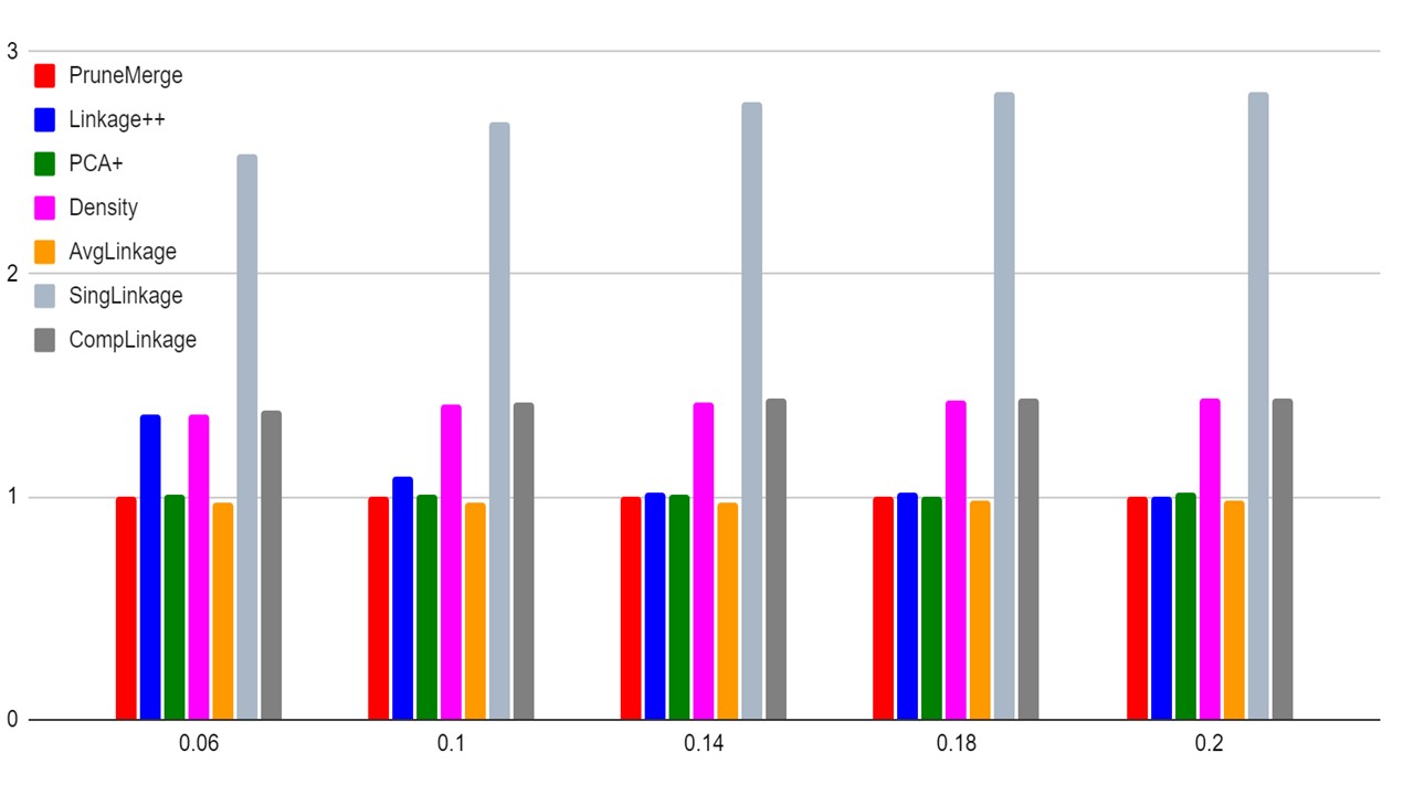
(a)

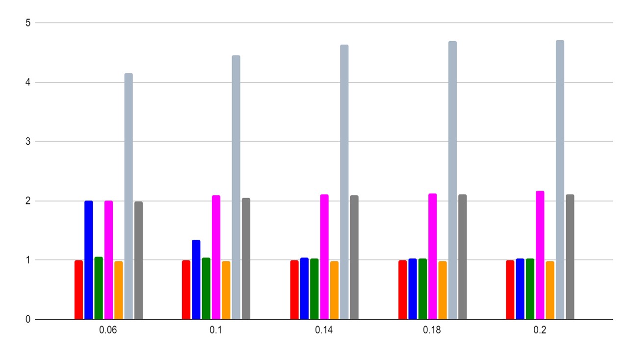
(b)

Figure 7: Results for clusters of the same size. The $x$-axis represents different values of $p$, while the $y$-axis represents the cost of the algorithms’ returned HC trees normalised by the cost of PruneMerge. Figure (a) corresponds to inputs generated according to the SBM, while Figure (b) corresponds to those generated according to the HSBM.

Clusters with non-uniform densities.

Next we study graphs in which edges are present non-uniformly within each cluster (e.g., Figure 1(a) discussed earlier). Specifically, we set $k=3,|P_{i}|=1000,q=0.002$, $p=0.06$, and every pair of vertices $(u,v)\in P_{i}\times P_{j}$ is connected by an edge with probability $p$ if $i=j$ and probability $q$ otherwise. Moreover, we choose a random set $S_{i}\subset P_{i}$ of size $|S_{i}|=c_{p}\cdot|P_{i}|$ from each cluster, and add edges to connect every pair of vertices in each $S_{i}$ so that the vertices of each $S_{i}$ form a clique. By setting different values of $c_{p}\in[0.05,0.4]$, the performance of our algorithm is about $20\%$ – $50\%$ better than Linkage++ with respect to the cost value of the constructed tree, see Figure 8(a) for detailed results. To explain the outperformance of our algorithm, notice that, by adding a clique into some cluster, the cluster structure is usually preserved with respect to $(\Phi_{\mathrm{in}},\Phi_{\mathrm{out}})$ or similar eigen-gap assumptions on well-clustered graphs. However, the existence of such a clique within some cluster would make the vertices’ degrees highly unbalanced; as such many clustering algorithms that involve the matrix perturbation theory in their analysis might not work well.

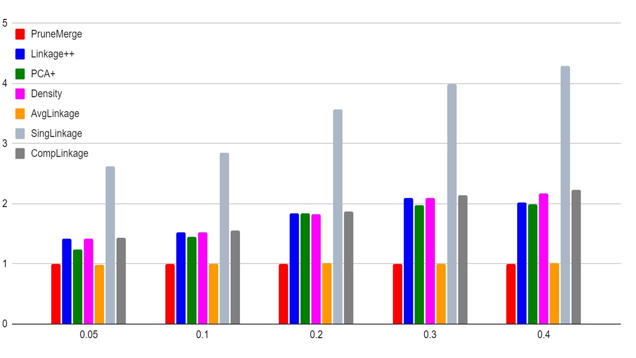
(a)

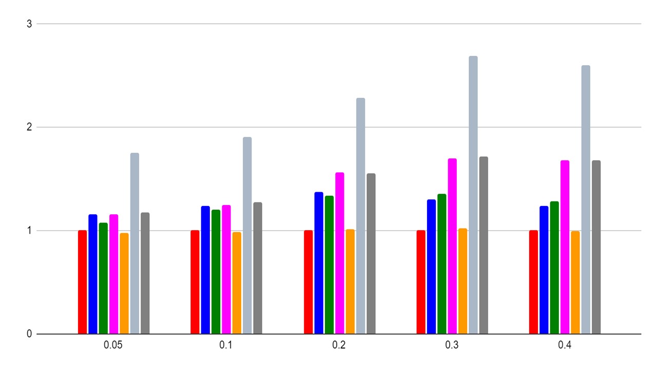
(b)

Figure 8: Results for graphs with non-uniform densities, or different sizes. The $x$-axis represents the $c_{p}$-values, while the $y$-axis represents the cost of the algorithms’ constructed trees normalised by the cost of the ones constructed by PruneMerge. Figure (a) corresponds to inputs where all clusters have the same size, while in Figure (b) the clusters have different sizes.

Clusters of different sizes.

To further highlight the significance of our algorithm on synthetic graphs of non-symmetric structures among the clusters, we study the graphs in which the clusters have different sizes. We choose the same set of $k$ and $q$ values as before ($k=3,q=0.002$), but set the sizes of the clusters to be $|P_{1}|=1900,|P_{2}|=900$ and $|P_{3}|=200$. Every pair of vertices $u,v\in P_{i}$, for $i\in\{1,2\}$ is connected by an edge with probability $p_{1}=0.06$, while pairs of vertices $u,v\in P_{3}$ are connected with probability $p_{2}=5\cdot p_{1}=0.3$. We further plant a clique $S_{i}\subset P_{i}$ of size $|S_{i}|=c_{p}\cdot P_{i}$ for each cluster $P_{i}$, as in the previous set of experiments. By choosing different values of $c_{p}$ from $[0.05,0.4]$, our results are reported in Figure 8(b), demonstrating that our algorithm performs better than the ones in [CAKMT17].

5.2 Experiments on real-world data sets

To evaluate the performance of our algorithm on real-world data sets, we follow the sequence of recent work on hierarchical clustering [ACAH19, CAKMT17, MRS⁺19, RP17], all of which are based on the following 5 data sets from the Scikit-learn library [PVG⁺11] as well as the UCI ML repository [UCI]: Iris, Wine, Cancer, Boston and Newsgroup. Similar with [RP17], for each data set we construct the similarity graph based on the Gaussian kernel, in which the $\sigma$-value is chosen according to the standard heuristic [NJW01]. As reported in Figure 9, our algorithm performs marginally worse than Linkage++ and significantly better than PCA+.

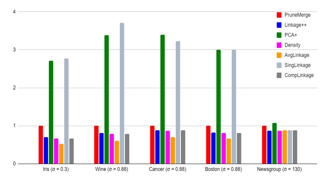
Figure 9: Results on real-world data sets. The $x$-axis represents the various data sets and our choice of the $\sigma$-value used for constructing the similarity graphs. The $y$-axis corresponds to the cost of the algorithms’ output normalised by the cost of PruneMerge.

6 Conclusion

Our experimental results on synthetic data sets demonstrate that our presented algorithm PruneMerge not only has excellent theoretical guarantees, but also produces output of lower cost than the previous algorithm Linkage++. In particular, the outperformance of our algorithm is best illustrated on graphs whose clusters have asymmetric internal structure and non-uniform densities. On the other side, our experimental results on real-world data sets show that the performance of PruneMerge is inferior to Linkage++ and especially to Average Linkage. We believe that developing more efficient algorithms for well-clustered graphs is a very meaningful direction for future work.

Finally, our experimental results indicate that the Average Linkage algorithm performs extremely well on all tested instances, when compared to PruneMerge and Linkage++. This leads to the open question whether Average Linkage achieves an $O(1)$-approximation for well-clustered graphs, although it fails to achieve this for general graphs [CAKMTM19]. In our point of view, the answer to this question could help us design more efficient algorithms for hierarchical clustering that not only work in practice, but also have rigorous theoretical guarantees.

References

- [AAV20] Noga Alon, Yossi Azar, and Danny Vainstein. Hierarchical clustering: a 0.585 revenue approximation. In 33rd Annual Conference on Learning Theory (COLT’20), pages 153–162, 2020.
- [ABS15] Sanjeev Arora, Boaz Barak, and David Steurer. Subexponential algorithms for unique games and related problems. Journal of the ACM, 62(5), 2015.
- [ACAH19] Amir Abboud, Vincent Cohen-Addad, and Hussein Houdrouge. Subquadratic high-dimensional hierarchical clustering. In 33rd Advances in Neural Information Processing Systems (NeurIPS’19), pages 11576–11586, 2019.
- [AKK+08] Sanjeev Arora, Subhash Khot, Alexandra Kolla, David Steurer, Madhur Tulsiani, and Nisheeth K. Vishnoi. Unique games on expanding constraint graphs are easy: extended abstract. In 40th Annual ACM Symposium on Theory of Computing (STOC’08), pages 21–28, 2008.
- [Alo86] N. Alon. Eigenvalues and expanders. Combinatorica, 6(2):83–96, 1986.
- [ARV09] Sanjeev Arora, Satish Rao, and Umesh Vazirani. Expander flows, geometric embeddings and graph partitioning. Journal of the ACM, 56(2):1–37, 2009.
- [CAKMT17] Vincent Cohen-Addad, Varun Kanade, and Frederik Mallmann-Trenn. Hierarchical clustering beyond the worst-case. In 31st Advances in Neural Information Processing Systems (NeurIPS’17), pages 6201–6209, 2017.
- [CAKMTM19] Vincent Cohen-Addad, Varun Kanade, Frederik Mallmann-Trenn, and Claire Mathieu. Hierarchical clustering: Objective functions and algorithms. Journal of the ACM, 66(4):1–42, 2019.
- [CC17] Moses Charikar and Vaggos Chatziafratis. Approximate hierarchical clustering via sparsest cut and spreading metrics. In 28th Annual ACM-SIAM Symposium on Discrete Algorithms (SODA’17), pages 841–854, 2017.
- [CCN19] Moses Charikar, Vaggos Chatziafratis, and Rad Niazadeh. Hierarchical clustering better than average-linkage. In 30th Annual ACM-SIAM Symposium on Discrete Algorithms (SODA’19), pages 2291–2304, 2019.
- [CCNY19] Moses Charikar, Vaggos Chatziafratis, Rad Niazadeh, and Grigory Yaroslavtsev. Hierarchical clustering for euclidean data. In 22nd International Conference on Artificial Intelligence and Statistics (AISTATS’19), pages 2721–2730, 2019.
- [Chu97] Fan R.K. Chung. Spectral graph theory. 1997.
- [CYL+20] Vaggos Chatziafratis, Grigory Yaroslavtsev, Euiwoong Lee, Konstantin Makarychev, Sara Ahmadian, Alessandro Epasto, and Mohammad Mahdian. Bisect and conquer: Hierarchical clustering via max-uncut bisection. In 23rd International Conference on Artificial Intelligence and Statistics (AISTATS’20), pages 3121–3132, 2020.
- [Das16] Sanjoy Dasgupta. A cost function for similarity-based hierarchical clustering. In 48th Annual ACM Symposium on Theory of Computing (STOC’16), pages 118–127, 2016.
- [GT14] Shayan Oveis Gharan and Luca Trevisan. Partitioning into expanders. In 25th Annual ACM-SIAM Symposium on Discrete Algorithms (SODA’14), pages 1256–1266, 2014.
- [HLW06] Hoory, Linial, and Wigderson. Expander graphs and their applications. BAMS: Bulletin of the American Mathematical Society, 43, 2006.
- [Kol10] Alexandra Kolla. Spectral algorithms for unique games. In 25th Conference on Computational Complexity (CCC’10), pages 122–130, 2010.
- [KVV04] Ravi Kannan, Santosh S. Vempala, and Adrian Vetta. On clusterings: Good, bad and spectral. Journal of the ACM, 51(3):497–515, 2004.
- [LGT14] James R Lee, Shayan Oveis Gharan, and Luca Trevisan. Multiway spectral partitioning and higher-order cheeger inequalities. Journal of the ACM, 61(6):1–30, 2014.
- [LSZ19] Huan Li, He Sun, and Luca Zanetti. Hermitian Laplacians and a Cheeger inequality for the Max-2-Lin problem. In 27th Annual European Symposium on Algorithms (ESA’19), pages 71:1–71:14, 2019.
- [McS01] Frank McSherry. Spectral partitioning of random graphs. In 42nd Annual IEEE Symposium on Foundations of Computer Science (FOCS’01), pages 529–537, 2001.
- [MRS+19] Aditya Krishna Menon, Anand Rajagopalan, Baris Sumengen, Gui Citovsky, Qin Cao, and Sanjiv Kumar. Online hierarchical clustering approximations. arXiv:1909.09667, 2019.
- [MW17] Benjamin Moseley and Joshua Wang. Approximation bounds for hierarchical clustering: Average linkage, bisecting -means, and local search. In 31st Advances in Neural Information Processing Systems (NeurIPS’17), pages 3094–3103, 2017.
- [NJW01] Andrew Ng, Michael Jordan, and Yair Weiss. On spectral clustering: Analysis and an algorithm. In 15th Advances in Neural Information Processing Systems (NeurIPS’01), pages 849–856, 2001.
- [PSZ17] Richard Peng, He Sun, and Luca Zanetti. Partitioning well-clustered graphs: Spectral clustering works! SIAM Journal on Computing, 46(2):710–743, 2017.
- [PVG+11] F. Pedregosa, G. Varoquaux, A. Gramfort, V. Michel, B. Thirion, O. Grisel, M. Blondel, P. Prettenhofer, R. Weiss, V. Dubourg, J. Vanderplas, A. Passos, D. Cournapeau, M. Brucher, M. Perrot, and E. Duchesnay. Scikit-learn: Machine learning in Python. Journal of Machine Learning Research, 12:2825–2830, 2011.
- [RP17] Aurko Roy and Sebastian Pokutta. Hierarchical clustering via spreading metrics. The Journal of Machine Learning Research, 18(1):3077–3111, 2017.
- [SZ19] He Sun and Luca Zanetti. Distributed graph clustering and sparsification. ACM Transactions on Parallel Computing, 6(3):17:1–17:23, 2019.
- [UCI] UCI ML Repository. https://archive.ics.uci.edu/ml/index.php. Accessed: 2021-05-22.
- [VCC+21] Danny Vainstein, Vaggos Chatziafratis, Gui Citovsky, Anand Rajagopalan, Mohammad Mahdian, and Yossi Azar. Hierarchical clustering via sketches and hierarchical correlation clustering. In 24th International Conference on Artificial Intelligence and Statistics (AISTATS’21), pages 559–567, 2021.
- [vL07] Ulrike von Luxburg. A tutorial on spectral clustering. Statistics and Computing, 17(4):395–416, 2007.
- [ZLM13] Zeyuan Allen Zhu, Silvio Lattanzi, and Vahab S. Mirrokni. A local algorithm for finding well-connected clusters. In 30th International Conference on Machine Learning (ICML’13), pages 396–404, 2013.