Carrollian manifolds and null infinity:
A view from Cartan geometry

Abstract

We discuss three different (conformally) Carrollian geometries and their relation to null infinity from the unifying perspective of Cartan geometry. Null infinity per se comes with numerous redundancies in its intrinsic geometry and the two other Carrollian geometries can be recovered by making successive choices of gauge. This clarifies the extent to which one can think of null infinity as being a (strongly) Carrollian geometry and we investigate the implications for the corresponding Cartan geometries.

The perspective taken, which is that characteristic data for gravity at null infinity are equivalent to a Cartan geometry for the Poincaré group, gives a precise geometrical content to the fundamental fact that “gravitational radiation is the obstruction to having the Poincaré group as asymptotic symmetries”.

1 Introduction/Summary

Carrollian geometries naturally emerge as the ultra-relativistic limit $c\to 0$ of pseudo-Riemannian manifolds. [1, 2]. This parallels the appearance of Galilean geometry in the non-relativistic limit $c\to\infty$ and in some sense these are dual to each others [3]. Loosely speaking, while the Galilean limit forces null cones to spread out into degenerate planes of constant absolute time, in the Carrollian limit null cones collapse into degenerate lines of constant absolute space (figure 1).

Accordingly, the fundamental building block of any Carrollian geometry consists of a manifold $\mathscr{I}$ foliated by lines. The space of lines $\Sigma$ typically is a manifold and this results in a fibre bundle $\mathscr{I}\xrightarrow[]{\pi}\Sigma$. One obtains a Carrollian geometry $\left(\mathscr{I}\to\Sigma,n^{\mu},h_{\mu\nu}\right)$ if the foliation $\mathscr{I}\to\Sigma$ is generated by a preferred vector field $n^{\mu}$ and is complemented by a degenerate metric $h_{\mu\nu}$ with one-dimensional kernel spanned by $n^{\mu}$.

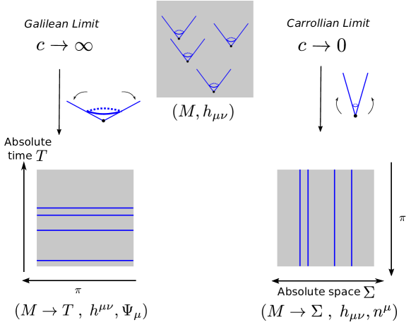
Figure 1: Galilean (non-relativistic) versus Carrollian (ultra-relativistic) limit: As the speed of light goes to infinity/zero the tangent null cones degenerate into lines/hypersurfaces of constant absolute space/time

This type of structure naturally appears in many different contexts of physical interest. They typically result of a limiting process or appear as the geometry induced on a null hypersurface. Applications include Hamiltonian analysis [4], Carrollian particles [5, 6], ultra-relativistic fluid mechanics [7, 8, 9, 10, 11, 12, 13], cosmology [14], Carrollian [15, 16, 17, 18, 19] and conformally Carrollian [20, 21, 22, 23] field theories, higher-spin [24, 25, 26], super-symmetric [27, 28, 29, 30, 31, 32] and non-commutative [33] extensions, null hypersurfaces and isolated horizons [34, 35, 36, 37, 38, 39, 40, 41, 42, 43, 44, 45], geometry of space/time-like infinities [46, 47, 48] and, finally, geometry of null infinity which is the main concern of this article.

It is a well-known fact that the conformal boundary of an asymptotically flat spacetime, which we will generically refer to as “null infinity”, is a (conformal) Carrollian manifold. There is in fact a precise sense in which flat limits of an asymptotically AdS spacetime correspond to ultra-relativistic contractions of the boundary [49].

The gravitational characteristic data however induce on null infinity much more than a mere Carrollian geometry [50, 51, 52]. In four dimensions this geometry is especially rich and e.g. is closely related to asymptotic twistors [53, 54] and Newman’s H-space [55, 56].

Depending on the perspective taken, especially the extent to which one wishes to preserve covariance and conformal invariance, there are various ways to describe the induced geometry. The purpose of this article is to discuss these in a coherent form emphasising their differences and relationships by framing them in the context of Cartan geometry.

Cartan geometry is a powerful organising tool in this context because the different views on the geometry of null infinity can in fact be captured by various homogeneous spaces which are all (conformal) Carrollian geometries with topology $\mathbb{R}\times S^{2}$. Cartan geometry amounts to making these models curved and thus capture the corresponding local geometry (This is closely related to the “gauging” procedure common in physics, see [57, 58] for pedagogical physicist-oriented introductions and [59, 60] for standard references). These homogeneous models are simple enough to be presented in this introduction; the detailed discussion of the corresponding curved geometries will form the core of this article.

Before discussing null infinity, it is instructive to consider the simpler model given by three-dimensional homogeneous Carrollian–de Sitter spacetime [2, 61]:

$$Carr_{dS}^{(3)}:=\faktor{\operatorname{Carr\!}_{dS}\left(3\right)}{\operatorname{ISO\!}\left(2\right)}.$$ (1.1)

This is an homogeneous space for the Carroll–de Sitter group $\operatorname{Carr\!}_{dS}\left(3\right):=\mathbb{R}^{3}\rtimes\operatorname{SO\!}\left(3\right)$ (with the stabiliser $\operatorname{ISO\!}\left(2\right)$ corresponding to a combination of rotations and Carrollian boosts). It can be obtained as the ultra-relativistic limit of $dS^{(3)}$, and therefore by construction is a Carrollian geometry. It is also equipped with a preferred compatible connection $\nabla$ and altogether this defines, in the terminology of [3], a strongly Carrollian geometry $\left(\mathscr{I}\to\Sigma,n^{\mu},h_{\mu\nu},\nabla\right)$. In fact, as we will show in the first section of this article, strongly Carrollian geometries are in one-to-one correspondence with Cartan geometry modelled on (1.1). What is more, we will obtain a result which applies uniformly to all dimensions $n\geq 2$ and all possible cosmological constant i.e. Carroll–De Sitter, Carroll and Carroll–Anti De Sitter. Taking the cosmological constant to zero one recovers the results from [62], restricting to dimension $2+1$ those of [24, 28, 63] and imposing a flatness condition the ones from [64].

The model for null infinity is, without surprise, an homogeneous space for the (connected component of the) Poincaré group $\operatorname{ISO\!}\left(3,1\right)=\mathbb{R}^{4}\rtimes\operatorname{SO\!}\left(3,1\right)_{0}$,

$$\mathscr{I}^{(3)}:=\faktor{\mathbb{R}^{4}\rtimes\operatorname{SO\!}\left(3,1\right)_{0}}{\mathbb{R}^{3}\rtimes\left(\mathbb{R}^{*}\times\operatorname{ISO\!}\left(2\right)\right)}.$$ (1.2)

The stabiliser now is a combination of rotations, Carrollian boosts and dilatations, corresponding to $\mathbb{R}^{*}\times\operatorname{ISO\!}\left(2\right)$, in semi-direct product with Carrollian special conformal transformations $\mathbb{R}^{3}$. There is an essential difference with the previous model: The appearance of $\operatorname{SO\!}\left(3,1\right)_{0}$, the conformal group of the two-sphere, means that this second model is only equipped with a conformal Carrollian geometry [65]. This well-known fact is related to the appearance of the BMS group [66, 67, 68, 69] as symmetries of asymptotically flat spacetimes. On top of being conformally Carrollian, the model for null infinity (1.2) is equipped with a Poincaré operator [70]: this is a differential operator $\mathcal{P}$ acting on densities and generalizing the Möbius operator of two-dimensional conformal geometry [71, 72]. This operator essentially corresponds to the possibility of defining (generalised) good-cut equations [55, 73]. In the spirit of [3] the data $\left(\mathscr{I}\to\Sigma,[n^{\mu},h_{\mu\nu}],\mathcal{P}\right)$ will be called strongly conformally Carrollian. As we will recall in our second section, strongly conformally Carrollian geometries are in one-to-one correspondence [70] with Cartan geometry modelled on (1.2). We will in fact recover these results from a more general (as compare to [70]) first order formalism that will encompass previous results and allows for a closer comparison with GHP-type formalisms [74, 75, 76] and closely related Ehresmann connections [11, 68, 10, 12].

To further compare similitudes and differences between (1.1) and (1.2), it is instructive to introduce a third homogeneous Carrollian manifold with topology $\mathbb{R}\times S^{2}$:

$$\mathscr{I}_{B}^{(3)}:=\faktor{\mathbb{R}^{4}\rtimes\operatorname{SO\!}\left(3\right)}{\mathbb{R}\times\operatorname{ISO\!}\left(2\right)}.$$ (1.3)

The abelian factor in the denominator is a remaining Carrollian special conformal transformation; we will soon discuss its geometrical meaning. This model bridges between the two previous ones in the sense that we have the following maps

$$\mathscr{I}^{(3)}\quad\to\quad\mathscr{I}^{(3)}_{B}\quad\to\quad Carr_{dS}^{(3)}.$$

The first map is rather natural: it is obtained by choosing an isometry subgroup $\operatorname{SO\!}\left(3\right)$ inside the conformal group $\operatorname{SO\!}\left(3,1\right)$ i.e. by picking up a round sphere representative in the conformal class of metric on $S^{2}$. Accordingly $\mathscr{I}_{B}^{(3)}$ is a model for null infinity in Bondi gauge (by which we really mean null infinity with a fixed constant curvature metric representative for the 2D metric). The second map is obtained by noting that

$$\mathscr{I}_{B}^{(3)}=\faktor{\mathbb{R}\times\operatorname{Carr\!}_{dS}\left(3\right)}{\mathbb{R}\times\operatorname{ISO\!}\left(2\right)}$$ (1.4)

and “forgetting” about the overall abelian factors. Note that, contrary to what the above expression might suggests, the $\mathbb{R}$ factor does act non trivially on the homogeneous space and there is no canonical way to perform this last step. The significance of this is the following: working in Bondi gauge, the geometry of the characteristic data at null infinity can be understood as a Carrollian geometry supplemented by an equivalence class $[\nabla]$ of compatible connections [51, 67, 77] and the extra abelian factor in the denominator of (1.4) takes one representative on another $\nabla\mapsto\nabla+fh_{\rho\nu}n^{\mu}$, $f\in\mathcal{C}^{\infty}\left(\mathscr{I}\right)$. Going from (1.4) to (1.1) amounts to choosing a preferred connection with constant curvature in the equivalence class. This sequence of gauge choices, leading from strongly conformally Carrollian to strong Carrollian geometries, is summarized in Table 1. More details, especially on how these choices can be understood from the perspective of the corresponding Cartan geometries, will be given in the last section of this article.

Table 1: Summary

Let us close this introduction by emphasising the conceptual implications of these results for the physics of gravitational radiation. As we already discussed, characteristic data for gravity at null infinity precisely correspond to Cartan geometries modelled on (1.2), prior to any gauge fixing, or to other models (1.1),(1.4) after suitable choice of gauge. The curvature of the Cartan connection in fact matches [78] the Newman-Penrose coefficients $\Psi^{0}_{4}$, $\Psi^{0}_{3}$, $Im\left(\Psi^{0}_{2}\right)$ and therefore invariantly encodes the presence of gravitational radiation at null infinity. The significance of this fact comes from the fundamental theorem of Cartan geometry:

Theorem 1.1.

Fundamental theorem of Cartan geometry (see e.g. [59])
Let $\left(\mathcal{G}\to M,\omega\right)$ be a Cartan geometry modelled on $G/H$, the curvature $d\omega+\tfrac{1}{2}[\omega,\omega]$ vanishes if and only if the geometry is locally isomorphic to the model $\left(G\to G/H,\omega_{G}\right)$.

In other terms, gravitational radiation is the obstruction to the existence of an isomorphism between null infinity and the model (1.2). The use of Cartan geometry thus reveals the deep connection between gravitational waves and the BMS group: radiation at null infinity is the obstruction (in the precise sense of Theorem 1.1) to being able to single out a preferred Poincaré group inside the BMS group. This well-known fact, which is of fundamental importance [79, 80, 81] here appears in a transparent form and has the value of a mathematical theorem.

It also follows that in the absence of gravitational radiation the geometry of null infinity is equivalent to a flat Cartan connection, which by the fundamental theorem of Cartan geometry, is equivalent to an isomorphism from null infinity to the model. These are not unique and the space of all such isomorphisms physically correspond to inequivalent gravity vacua on which the BMS group act transitively [82, 77, 70]. This degeneracy of gravity vacua is tightly related to the existence of memory effect in general relativity [83, 84, 67, 85] and has deep implications for the quantum gravity S-matrix [86, 87, 77] as well as the black-hole information paradox [88]. Finally, since gravity vacua correspond to flat Cartan connections on $\mathscr{I}$ it is natural to think of the corresponding Chern-Simon functional at null infinity [89] as some sort of effective boundary theory (see also [90] for more tractor actions for gravity).

This article is organised as follows: In a first section we discuss the correspondence between strong Carrollian geometries and Cartan geometry modelled on (1.1). In a second section we investigate the invariant geometry of null infinity as Cartan geometry modelled on (1.2). Finally we compare these two realisations by considering null infinity in Bondi gauge, i.e. for which one has singled out a preferred constant curvature representative from the conformal class.

2 Carrollian spacetimes

Let $\mathscr{I}$ be a manifold foliated by lines. This will be convenient (but not necessary) to suppose that the space of lines $\Sigma$ is a manifold and that consequently $\mathscr{I}\xrightarrow[]{\pi}\Sigma$ is a fibre bundle . We will also suppose that the lines are generated by a (nowhere vanishing) vector field $n^{\mu}$. The flow generated by this vector field equips (at least locally) Carrollian geometry with a preferred time $u\colon U\subset\mathscr{I}\to\mathbb{R}$ which is unique up to “super-translations”

$$u\mapsto u+\pi^{*}\xi,\qquad\xi\in\mathcal{C}^{\infty}\left(\Sigma\right).$$ (2.1)

Definition 2.1.

A Carrollian geometry [3] $\left(\mathscr{I}\to\Sigma,n^{\mu},h_{\mu\nu}\right)$ is the data of a one-dimensional fibre bundle $\mathscr{I}\to\Sigma$ together with a nowhere vanishing vector field $n^{\mu}$ generating the foliation and a degenerate metric $h_{\mu\nu}$ with one-dimensional kernel such that

$$h_{\mu\nu}n^{\nu} =0, \mathcal{L}_{n}h_{\mu\nu} =0.$$ (2.2)

The above requirements mean that $h_{\mu\nu}$ defines a genuine metric (i.e. invertible) on $\Sigma$. This definition has the advantage that Carrollian geometries then always have a non-trivial automorphism algebra given by the semi-direct product of super-translations $\mathcal{T}\simeq\mathcal{C}^{\infty}\left(\Sigma\right)$ with isometries of $\left(\Sigma,h_{\mu\nu}\right)$

$$\textrm{Lie}\left(\operatorname{ISO\!}\left(\mathscr{I}\to\Sigma,n^{\mu},h_{\mu\nu}\right)\right)\simeq\textrm{Lie}\left(\mathcal{T}\rtimes\operatorname{ISO\!}\left(\Sigma,h_{\mu\nu}\right)\right).$$ (2.3)

This isomorphism is obtained by making a choice of local trivialisation (i.e. time). For instance, if $\left(\Sigma,h_{\mu\nu}\right)=\left(\mathbb{R}^{n-1},dy^{A}dy^{B}\delta_{AB}\right)$ is flat euclidean space and $\mathscr{I}=\mathbb{R}\times\Sigma$ then symmetries are the semi-direct product of super-translations with euclidean isometries $\operatorname{ISO\!}\left(n-1\right)=\mathbb{R}^{n-1}\rtimes\operatorname{SO\!}\left(n-1\right)$.

Even though the second condition in (2.2) is too restrictive to encompass all geometries obtained by ultra-relativistic contractions, essential gravitational realisations are nonetheless of this type: prototypical examples are Killing horizons and null infinity in Bondi gauge. It should however be noted that the above definition does not encompass generic (non-Killing) null hypersurfaces for which there is no preferred vector field $n^{\mu}$, see [35] for a detailed discussion on alternative definitions modelling various type of horizons. A close inspection shows that none of the results in this section actually relies on the second requirement in (2.2).

In this section we will discuss strongly Carrollian geometries [3] (see [91] for a comprehensive discussion) and describe the related Cartan geometries for a generic dimension and cosmological constant i.e. for Cartan geometries modelled on Carroll–De Sitter, Carroll and Carroll–Anti De Sitter. Taking the cosmological constant to zero we will recover results from [62], restricting the arbitrary dimension to $2+1$ results of [24, 28, 63] and imposing a flatness condition those of [64]. The main results are summarized in table 2.

Table 2: Cartan geometry of Carrollian spacetimes

Model
Carroll–De Sitter spacetime, $\Lambda>0$ $\faktor{\operatorname{Carr\!}_{dS}\left(n\right)}{\operatorname{ISO\!}\left(n-1\right)}$ $\simeq\mathbb{R}\times S^{n-1}$ Carroll spacetime, $\Lambda=0$ $\faktor{\operatorname{Carr\!}\left(n\right)}{\operatorname{ISO\!}\left(n-1\right)}$ $\simeq\mathbb{R}\times\mathbb{R}^{n-1}$ Carroll–anti De Sitter spacetime, $\Lambda<0$ $\faktor{\operatorname{Carr\!}_{AdS}\left(n\right)}{\operatorname{ISO\!}\left(n-1\right)}$ $\simeq\mathbb{R}\times H^{n-1}$
(Weak) Carrollian geometry
$\left(\mathscr{I}\to\Sigma,n^{\mu},h_{\mu\nu}\right)$	defines a canonical	$\operatorname{ISO\!}\left(n-1\right)$-principal bundle
	has symmetry group	$\mathcal{C}^{\infty}\left(\Sigma\right)\rtimes\operatorname{ISO\!}\left(\Sigma,h_{\mu\nu}\right)$
Strong Carrollian geometry
$\left(\mathscr{I}\to\Sigma,n^{\mu},h_{\mu\nu},\nabla\right)$	defines a unique	$\mathfrak{carr}_{\Lambda}\left(n\right)$-valued connection $D$
Flatness of $D$	reduces the symmetry group to	$\operatorname{Carr\!}_{\Lambda}\left(n\right)$.

2.1 Homogeneous model

The “Carrollian isometry groups” are obtained by ultra-relativistic contractions of the isometry group of de Sitter, flat, and anti de Sitter spacetimes in $n$ dimensions [1, 2]. The corresponding groups are respectively called Carroll–de Sitter, Carroll and Carroll–anti de Sitter. We will use the compact notation $Carr_{\Lambda}\left(n\right)$ for representing these three groups,

$$\operatorname{Carr\!}_{dS}\left(n\right) =\operatorname{Carr\!}_{\Lambda>0}\left(n\right), \operatorname{Carr\!}\left(n\right) =\operatorname{Carr\!}_{\Lambda=0}\left(n\right), \operatorname{Carr\!}_{AdS}\left(n\right) =\operatorname{Carr\!}_{\Lambda<0}\left(n\right).$$

We then have

$$\operatorname{Carr\!}_{\Lambda}\left(n\right):=\mathbb{R}^{n}\rtimes\operatorname{ISO\!}_{\Lambda}\left(n-1\right)$$ (2.4)

where it is convenient to introduce a single notation

$$\operatorname{ISO\!}_{\Lambda>0}\left(n-1\right) =\operatorname{SO\!}\left(n\right), \operatorname{ISO\!}_{\Lambda=0}\left(n-1\right) =\operatorname{ISO\!}\left(n-1\right), \operatorname{ISO\!}_{\Lambda<0}\left(n-1\right) =\operatorname{SO\!}\left(n-1,1\right)_{0}.$$ (2.5)

for the (connected component of) isometry groups of $S^{n-1}$ , $\mathbb{R}^{n-1}$ and $H^{n-1}$.

It is useful to think of $\operatorname{ISO\!}_{\Lambda}\left(n-1\right)$ as the subgroup of $\operatorname{SO\!}\left(n,1\right)_{0}$ stabilising a vector of norm $-2\Lambda$ (the factor of two is only introduced for future convenience). Making use of this fact, the Carrollian isometry groups can be represented matricially as

$$\operatorname{Carr\!}_{\Lambda}\left(n\right)=\left\{\quad\begin{pmatrix}m^{i}{}_{j}&0\\ t_{i}&1\end{pmatrix}\quad\Big{|}\quad\begin{array}[]{c}m^{i}{}_{j}\in\operatorname{SO\!}\left(n,1\right)_{0},\;t_{i}\in\mathbb{R}^{n+1}\\[3.99994pt] \text{s.t.}\quad m^{i}{}_{j}I^{j}=I^{i},\,t_{i}I^{i}=0.\end{array}\quad\right\}$$ (2.8)

with $I^{i}\in\mathbb{R}^{n+1}$ a fixed vector of norm $-2\Lambda$. Introducing a null basis on $\mathbb{R}^{n+1}$ we write $I^{i}=\left(I^{+},I^{A},I^{-}\right)$ with $I^{A}\in\mathbb{R}^{n-1}$ and

$$I^{i}I^{j}\eta_{ij}=2I^{+}I^{-}+I^{A}I^{B}\delta_{AB}.$$

Without loss of generality we can take $I^{i}=\left(1,0^{A},-\Lambda\right)$. The Lie algebra $\mathfrak{carr}_{\Lambda}\left(n\right)$ is then generated by matrices of the form

$$\mathfrak{carr}_{\Lambda}\left(n\right)=\left\{\quad\begin{pmatrix}0&-m_{B}&0&0\\ \Lambda\,m^{A}&\mathfrak{m}^{A}{}_{B}&m^{A}&0\\ 0&-\Lambda\,m_{B}&0&0\\ \Lambda\,t_{-}&t_{B}&t_{-}&0\end{pmatrix}\quad\Big{|}\quad\begin{array}[]{c}\mathfrak{m}^{A}{}_{B}\in\mathfrak{so}(n-1),\;t_{B}\in\mathbb{R}^{n-1},\\[3.59995pt] (m^{A},t_{-})\in\mathbb{R}^{n}\end{array}\quad\right\}.$$ (2.11)

Spatial rotations and “Carrollian boosts” are respectively generated by $\mathfrak{m}^{A}{}_{B}$ and $t_{B}$, while the $n$ “Carrollian translations” are generated by $m^{A}$ and $t_{-}$. In this representation, the Carroll isometry groups naturally act on $\mathbb{R}^{n+2}$ with coordinates $Y^{I}=\left(Y^{+},Y^{A},Y^{-},Y^{0}\right)$ and degenerate metric

$$Y^{I}Y^{J}h_{IJ}=2Y^{+}Y^{-}+Y^{A}Y^{B}\delta_{AB}.$$ (2.12)

The homogeneous Carrollian spacetimes are then defined to be the quotient [2, 61, 64]

$$Carr^{(n)}_{\Lambda}:=\faktor{\operatorname{Carr\!}_{\Lambda}\left(n\right)}{\operatorname{ISO\!}\left(n-1\right)}.$$ (2.13)

Where $\operatorname{ISO\!}\left(n-1\right)$ is identified with the subgroup of $\operatorname{Carr\!}_{\Lambda}\left(n\right)$ stabilising $X^{I}=\left(0,0^{A},1,0\right)$,

$$\left\{\begin{pmatrix}1&0&0&0\\ 0&m^{A}{}_{B}&0&0\\ 0&0&1&0\\ 0&t_{B}&0&1\end{pmatrix}\quad\Big{|}\quad m^{A}{}_{B}\in\operatorname{SO\!}\left(n-1\right),t_{B}\in\mathbb{R}^{n-1}\quad\right\} \leq\operatorname{Carr\!}_{\Lambda}\left(n\right),$$ (2.14)

and therefore is generated by Carrollian boosts and rotations.

These models are the total space of a (trivial) line bundle over sphere/flat/hyperbolic spaces respectively (the degenerate metric is obtained by pull-back of the metric on the base) i.e. we have the isomorphisms

$$Carr^{(n)}_{dS} \simeq\mathbb{R}\times S^{n-1}, Carr^{(n)} \simeq\mathbb{R}\times\mathbb{R}^{n-1}, Carr^{(n)}_{AdS} \simeq\mathbb{R}\times H^{n-1}.$$

Alternatively, the model Carrollian spacetimes can be realised as

$$Carr^{(n)}_{\Lambda}=\left\{Y^{I}=\begin{pmatrix}Y^{+}\\ Y^{A}\\ Y^{-}\\ Y^{0}\end{pmatrix}\in\mathbb{R}^{n+2}\quad\big{|}\quad Y^{I}Y^{J}h_{IJ}=0,\quad Y^{I}I^{J}_{(\Lambda)}h_{IJ}=1\right\}$$ (2.15)

where $I^{I}_{(\Lambda)}:=\left(1,0^{A},-\Lambda,0\right)$ is a fixed vector of norm $-2\Lambda$ for the degenerate metric (2.12) (the Carrollian vector field is then proportional to $\partial_{Y^{0}}$). In particular, note that $X^{I}=\left(0,0^{A},1,0\right)$ always belongs to $Carr^{(n)}_{\Lambda}$. In order to identify (2.15) with the homogeneous space (2.13) it suffices to note that the Carrollian isometry groups act transitively and that the stabiliser of a point $X^{I}$ is $\operatorname{ISO\!}\left(n-1\right)$.

2.2 Tetrad formalism adapted to Carrollian geometry

Let $\left(\mathscr{I}\to\Sigma,n^{\mu},h_{\mu\nu}\right)$ be a Carrollian geometry as in Definition 2.1. Let $U$ be an open set of $\mathscr{I}$ and $\big{\{}e_{A}{}^{\mu}\big{\}}_{A\in 1,\,...\,,n-1}$, be vector fields on this set. We will say that $\left\{e_{a}{}^{\mu}\right\}_{a\in 1,\,...\,,n}=\left\{e_{A}{}^{\mu},n^{\mu}\right\}_{A\in 1,\,...\,,n-1}$ is an orthogonal frame or “tetrad” if it forms a basis of the tangent bundle at any $x\in U$ and satisfies

$$e_{A}{}^{\mu}e_{B}{}^{\nu}h_{\mu\nu} =\delta_{AB}$$

where $\delta_{AB}$ is the identity matrix. Tetrads have a $\operatorname{ISO\!}\left(n-1\right)$-ambiguity

$$\begin{array}[]{lcl}e_{A}{}^{\mu}&\mapsto&m_{A}{}^{B}\left(e_{B}{}^{\mu}-t_{B}n^{\mu}\right)\\ n^{\mu}&\mapsto&n^{\mu}\end{array} \begin{pmatrix}m^{A}{}_{B}&0\\ t_{B}&1\end{pmatrix} \in\operatorname{ISO\!}\left(n-1\right).$$ (2.18)

Carrollian geometries are therefore canonically equipped with a $\operatorname{ISO\!}\left(n-1\right)$-principal bundle obtained from the reduction of the frame bundle of $\mathscr{I}$ to such tetrads. These local symmetries are respectively interpreted as spatial rotations (for those generated by $\operatorname{SO\!}\left(n-1\right)$) and “Carrollian boosts” (generated by $\mathbb{R}^{n-1}$).

We will write the corresponding dual tetrad $\left\{\theta_{\mu}{}^{a}\right\}_{a\in 1,\,...\,,n}=\left\{\theta_{\mu}{}^{A},l_{\mu}\right\}_{A\in 1,\,...\,,n-1}$:

$$e_{B}{}^{\mu}\theta_{\mu}{}^{A} =\delta_{B}{}^{A}, n^{\mu}\theta_{\mu}{}^{A} =0, e_{B}{}^{\mu}l_{\mu} =0, n^{\mu}l_{\mu} =1.$$

In what follows, it will be important that, under the action of $\operatorname{ISO\!}\left(n-1\right)$, dual tetrads transform as

$$\theta_{\mu}{}^{A} \mapsto m^{A}{}_{B}\;\theta_{\mu}{}^{B}, l_{\mu} \mapsto l_{\mu}+t_{C}\;\theta_{\mu}{}^{C}.$$ (2.19)

2.3 Strongly Carrollian geometry

Let $\left(\mathscr{I}\to\Sigma,n^{\mu},h_{\mu\nu}\right)$ be a Carrollian geometry. We will say that it is strongly Carrollian [3, 91] if, on top of this, it is equipped with a torsion-free connection $\nabla_{\rho}$ on the tangent bundle satisfying the compatibility relations

$$\nabla_{\rho}n^{\mu} =0, \nabla_{\rho}h_{\mu\nu} =0.$$ (2.20)

The components of this connection in a tetrad $\left\{e_{A}{}^{\mu},n^{\mu}\right\}$ are

$$\begin{pmatrix}\theta_{\mu}{}^{A}\nabla_{\rho}e_{B}^{\mu}&\theta_{\mu}{}^{A}\nabla_{\rho}n^{\mu}\\ l_{\mu}\nabla_{\rho}e_{B}^{\mu}&l_{\mu}\nabla_{\rho}n^{\mu}\end{pmatrix}=\begin{pmatrix}\omega_{\rho}{}^{A}{}_{B}&0\\ -\tfrac{1}{2}C_{B}{}_{\rho}&0\end{pmatrix}$$ (2.21)

(the minus one half factor is here added to fit with notation from the literature [94, 78]) and the torsion-free condition is

$$d^{\nabla}\left(\theta^{a}e_{a}{}^{\mu}\right):=d^{\omega}\theta^{A}\;e_{A}^{\mu}+\left(dl-\tfrac{1}{2}C{}_{B}\wedge\theta^{B}\right)n^{\mu}=0$$

where we introduced the notation $d^{\omega}\theta^{A}:=d\theta^{A}+\omega^{A}{}_{B}\wedge\theta^{B}$. It follows that $\omega_{\rho}{}^{A}{}_{B}$ is uniquely determined in terms of $\theta^{A}_{\mu}$. On the other hand, the coefficients

$$C_{AB}\;\theta_{\mu}{}^{B}+C_{A0}\,l_{\mu} :=C_{A}{}_{\mu}$$

are only fixed in terms of the tetrad up to

$$C_{A}{}_{\mu}\mapsto C_{A}{}_{\mu}+\delta C_{AB}\;\theta_{\mu}{}^{B}$$

where $\delta C_{AB}$ is a symmetric tensor, $\delta C_{AB}=\delta C_{(AB)}$. This remaining freedom corresponds to the information contained in the strongly Carrollian geometry $\left(\mathscr{I}\to\Sigma,n^{\mu},h_{\mu\nu},\nabla\right)$ as opposed to the bare Carrollian geometry $\left(\mathscr{I}\to\Sigma,n^{\mu},h_{\mu\nu}\right)$.

2.4 The Carrollian Cartan connection

Carrollian spacetimes are tightly related to the geometry of $\mathfrak{carr}_{\Lambda}$-valued connections (see e.g. [62, 24, 63, 64]).

Let $\left(\mathscr{I}\to\Sigma,n^{\mu},h_{\mu\nu}\right)$ be a Carrollian geometry. Corresponding tetrads then form an $\operatorname{ISO\!}\left(n-1\right)$-principal bundle and we will call (Carrollian) tractors (following the terminology of [95, 60]) sections $\Phi^{I}$ of the associated bundle for the representation (2.14).

Let $D_{\rho}$ be a generic connection valued in the Carroll Lie algebra (2.11), it acts on tractors as

$$D\Phi^{I}=\begin{pmatrix}d&-\theta_{B}&0&0\\ \Lambda\,\theta^{A}&d^{\omega}&\theta^{A}&0\\ 0&-\Lambda\,\theta_{B}&d&0\\ \Lambda\,l&-\tfrac{1}{2}C_{B}&l&d\end{pmatrix}\begin{pmatrix}\Phi^{+}\\ \Phi^{B}\\ \Phi^{-}\\ \Phi^{0}\end{pmatrix}.$$

Changes of tetrad (2.18) are equivalent to gauge transformations with values in $\operatorname{ISO\!}\left(n-1\right)$ (in the representation (2.14)) and induce the following transformation on the connection components

$$\theta^{A} \mapsto m^{A}{}_{B}\theta^{B}, l \mapsto l+\theta^{C}t_{C},$$

$$\omega^{A}{}_{B} \mapsto m^{A}{}_{C}\omega^{C}{}_{D}m_{B}{}^{D}-dm^{A}{}_{C}m_{B}{}^{C}, -\tfrac{1}{2}C_{A} \mapsto m_{A}{}^{B}\left(-\tfrac{1}{2}C_{B}-d^{\omega}t_{B}\right).$$ (2.22)

We will say that such a connection is compatible with the Carrollian geometry if $\left\{\theta_{\mu}{}^{A},l_{\mu}\right\}$ defines a dual-tetrad. The curvature of the connection is

$$F^{I}{}_{J}=\begin{pmatrix}0&-d^{\omega}\theta_{B}&0&0\\ \Lambda\,d^{\omega}\theta^{A}&F^{A}{}_{B}-2\Lambda\,\theta^{A}\wedge\theta_{B}&d^{\omega}\theta^{A}&0\\ 0&-\Lambda\,d^{\omega}\theta_{B}&0&0\\ \Lambda\left(dl-\tfrac{1}{2}C_{C}\wedge\theta^{C}\right)&-\tfrac{1}{2}d^{\omega}C_{B}-2\Lambda\,l\wedge\theta_{B}&dl-\tfrac{1}{2}C_{C}\wedge\theta^{C}&0\end{pmatrix}.$$

In particular $\left(\omega^{A}{}_{B},C_{B}\right)$ are the components of a torsion-free connection $\nabla$ if and only if $F^{I}{}_{-}=0$. We will say that such $\mathfrak{carr}_{\Lambda}\left(n\right)$-valued connections are torsion-free.

We thus derived the following, generalizing results from [62]:

Proposition 2.1.

Let $\left(\mathscr{I}\to\Sigma,n^{\mu},h_{\mu\nu}\right)$ be a $n$-dimensional Carrollian geometry, there is a one-to-one correspondence between, on the one hand, $\mathfrak{carr}\left(n\right)$-valued connections which are both compatible with the Carroll geometry and torsion-free and, on the other hand, choice of strongly Carrollian geometries $\left(\mathscr{I}\to\Sigma,n^{\mu},h_{\mu\nu},\nabla\right)$.

It follows from the fundamental theorem of Cartan geometry (see theorem 1.1) that we have the

Proposition 2.2.

Let $\left(\mathscr{I}\to\Sigma,n^{\mu},h_{\mu\nu},\nabla\right)$ be a $n$-dimensional strongly Carrollian geometry satisfying

$$F^{A}{}_{B}-2\Lambda\;\theta^{A}\wedge\theta_{B} =0, -\tfrac{1}{2}d^{\omega}C_{B}-2\Lambda\;l\wedge\theta_{B} =0,$$

then $\mathscr{I}\to\Sigma$ is locally isomorphic to the model

$$Carr^{(n)}_{\Lambda}:=\faktor{\operatorname{Carr\!}_{\Lambda}\left(n\right)}{\operatorname{ISO\!}\left(n-1\right)}.$$

In particular, the algebra of local symmetries is $\mathfrak{carr}_{\Lambda}\left(n\right)$.

2.5 “Carrollian good-cuts”

2.5.1 BMS coordinates

We will call “BMS” coordinates $u\colon\mathscr{I}\to\mathbb{R}$ a local trivialisation of $\mathscr{I}\to\Sigma$ chosen such that $n^{\mu}(du)_{\mu}=1$ i.e. such that it defines an element of dual tetrad $l_{\mu}:=(du)_{\mu}$. This defines a unique tetrad $\{e_{A}{}^{\mu},n^{\mu}\}$ (up to $\operatorname{SO\!}\left(n-1\right)$) by requiring that $e_{A}^{\mu}(du)_{\mu}=0$. Changing the trivialisation $u\mapsto\hat{u}$ gives the following transformation rules

$$e_{A}{}^{\mu} \mapsto e_{A}{}^{\mu}-t_{A}n^{\mu}, t_{B} =\nabla_{B}\hat{u},$$

where $\nabla_{A}\hat{u}:=e_{A}^{\mu}\nabla_{\mu}\hat{u}$.

In BMS coordinates, $dl=0$ and the previous computation simplifies, for example normal Carrollian connections are then parametrised by $C_{A}=C_{(AB)}\theta^{B}$ and $\omega^{A}{}_{B}$ is just the pull-back of the Levi-Civita connection of $\left(\Sigma,h_{\mu\nu}\right)$ to $\mathscr{I}$.

2.5.2 Carrollian good-cuts

Let $\mathcal{G}\colon\Sigma\to\mathscr{I}$ be a section (or “cut”) of $\mathscr{I}$. Let $u$ be a BMS coordinate. We can always think of the cut $\mathcal{G}$ as the zero set of another BMS coordinate $f$ on $\mathscr{I}$,

$$f=u-\pi^{*}G$$

where $G\in\mathcal{C}^{\infty}\left(\Sigma\right)$ is a function on $\Sigma$ and the cut is given by $f=0$.

We will say that $\mathcal{G}$ is a Carrollian good-cut for a strongly Carrollian geometry $\left(\mathscr{I}\to\Sigma,n^{\mu},h_{\mu\nu},\nabla_{\rho}\right)$ if and only if

$$\nabla_{(\mu}\nabla_{\nu)}f\big{|}_{\mathcal{G}}=0.$$

In a tetrad given by $u$ this is equivalent to

$$\nabla_{(A}\nabla_{B)}G-\tfrac{1}{2}C_{AB}\big{|}_{u=G}=0.$$

(this follows from (2.21)). In the flat model (2.13) the space of Carrollian good-cut is $n$ dimensional and defines preferred time foliations on which the $n$ Carrollian translations act transitively.

These “Carrollian good-cuts” crucially differ from the usual good-cut equation [55, 96, 73, 97] of null-infinity

$$\left(\nabla_{(A}\nabla_{B)}G-\tfrac{1}{2}C_{AB}\big{|}_{u=G}\right)\big{|}_{tf}=0.$$

by a trace part (here $\big{|}_{tf}$ indicates “trace-free part of”). While the usual good-cut equation has at most $(n+1)$ independent solutions, the Carrollian good-cuts must satisfy one more equation and have a maximum of $n$ independent solutions. This is ultimately related to the fact that the homogenous realisation of Carrollian geometry (2.13) has $n$ Carrollian translations while the homogenous realisation of null-infinity (3.2) possess $n+1$ of these. This can be clarified by relating good-cuts to covariantly constant sections.

2.5.3 Covariantly constant sections

Let $\left(\mathscr{I}\to\Sigma,n^{\mu},h_{\mu\nu},\nabla\right)$ be a strongly Carrollian geometry and let $D$ be the corresponding Carroll-valued connection. Its action on dual elements is

$$D\Phi_{I}=\begin{pmatrix}d&-\theta^{B}&0&-l\\ \Lambda\theta_{A}&d^{\omega}&\theta_{A}&\tfrac{1}{2}C_{A}\\ 0&-\Lambda\theta^{B}&d&-l\Lambda\\ 0&0&0&d\end{pmatrix}\begin{pmatrix}\Phi_{-}\\ \Phi_{B}\\ \Phi_{+}\\ \Phi_{0}\end{pmatrix}$$

where duality is defined by $\Phi_{I}\Phi^{I}=\Phi_{+}\Phi^{+}+\Phi_{A}\Phi^{A}+\Phi_{-}\Phi^{-}+\Phi_{0}\Phi^{0}$. By construction the Carrollian connection stabilises the section $I_{(\Lambda)}^{I}=\left(1,0^{A},-\Lambda,0\right)$.

Let $\Phi_{I}=\left(f,\Phi_{A},\Phi_{+},\Phi_{0}\right)$ be a covariantly constant dual tractor $D_{\rho}\Phi_{I}=0$ satisfying $\Phi_{+}-\Lambda f=\Phi_{I}I^{I}_{(\Lambda)}=0$. A direct computation shows that this is equivalent to having $\Phi_{I}=\left(f,\nabla_{A}f,\Lambda f,\dot{f}\right)$ and

$$\nabla_{\mu}\dot{f} =0, \nabla_{(A}\nabla_{B)}f+\tfrac{1}{2}C_{(AB)}\dot{f}+2\Lambda f\;h_{AB} =0$$ (2.23)

where dot indicate Lie derivatives along $n^{\mu}$.

Let us pick a BMS coordinate $u\colon\mathscr{I}\to\mathbb{R}$. The above equations can be equivalently rewritten as

$$f =k\left(u-G\right), \nabla_{(A}\nabla_{B)}G-\tfrac{1}{2}C_{AB}-2\Lambda\left(u-G\right)\;h_{AB} =0,$$ (2.24)

where $G$ is a function on $\Sigma$ and $k\in\mathbb{R}$ is some constant. Evaluating the above equation at $u=G$ one finds that $\Phi_{I}$ is covariantly constant if and only if $G$ solves the Carrollian good cut equation and

$$\tfrac{1}{2}C_{AB}=-2\Lambda(u-G)h_{AB}+\tfrac{1}{2}C_{AB}\big{|}_{u=G}.$$

I.e. $\tfrac{1}{2}\dot{C}_{AB}=-2\Lambda h_{AB}$. This last condition amounts to the vanishing of one of the coefficient of the Carrollian curvature. When this is satisfied Carrollian good-cuts are in one-to-one correspondence with covariantly constant sections $\Phi_{I}$ which are orthogonal to $I_{\Lambda}^{I}$ and considered up to an overall scale. This is a space of finite dimension at most $n$ and this dimension is attained when the geometry is flat.

3 Null Infinity

Since null infinity is the conformal boundary of an asymptotically flat spacetime this must be some type of conformal manifold. This is in fact a conformal Carrollian geometry in the following sense.

Definition 3.1.

A conformal Carrollian geometry $\left(\mathscr{I}\to\Sigma,[n^{\mu},h_{\mu\nu}]\right)$ is the data of a $n$-dimensional fibre bundle $\mathscr{I}\to\Sigma$ over a $(n-1)$-dimensional manifold $\Sigma$ together with an equivalence class of vector fields and degenerate metrics with one-dimensional kernel

$$\left(n^{\mu},h_{\mu\nu}\right)\sim\left(\lambda^{-1}n^{\mu},\lambda^{2}h_{\mu\nu}\right),\quad\qquad\mathcal{C}^{\infty}\left(\mathscr{I}\right)\ni\lambda>0,$$

satisfying

$$n^{\nu}h_{\mu\nu} =0, \mathcal{L}_{n}h_{\mu\nu} =\Theta h_{\mu\nu},$$

where $\Theta:=\tfrac{1}{n-1}h^{\mu\nu}\mathcal{L}_{n}h_{\mu\nu}$.

The above definition means that $\left(\Sigma,[h_{\mu\nu}]\right)$ defines a conformal geometry in the usual sense. We stress, however, that in principle rescalings by functions $\lambda$ defined on the whole of $\mathscr{I}$ are allowed. As is well known [66, 67], the algebra of automorphisms of conformal Carrollian geometry is a generalised version of the BMS algebra.

$$\textrm{Lie}\left(\operatorname{ISO\!}\left(\mathscr{I}\to\Sigma,[n^{\mu},h_{\mu\nu}]\right)\right)\simeq\textrm{Lie}\left(\mathcal{T}\rtimes\operatorname{ISO\!}\left(\Sigma,[h_{\mu\nu}]\right)\right),$$ (3.1)

We recover the standard BMS group [79, 80, 81] by considering the case where $\left(\Sigma,[h_{\mu\nu}]\right)$ is the two-dimensional conformal sphere, $\textrm{BMS}_{4}\simeq\mathcal{T}\rtimes\operatorname{SO\!}\left(3,1\right)$. Note that choosing a representative $\left(\mathscr{I}\to\Sigma,n^{\mu},h_{\mu\nu}\right)$ such that $\mathcal{L}_{n}h_{\mu\nu}=0$ is always possible (these representatives are Carrollian geometries in the sense of Definition 2.1), we will call these “Bondi gauge” and discuss them in the next section.

Conformal geometry is typically a difficult subject because of the necessity of dealing with Weyl rescalings. Tractor calculus [95, 98] has been devised specifically to provide a manifestly “Weyl-rescaling invariant” formalism. In [70] these methods were extended to conformal Carrollian manifolds. We here keep developing this formalism, making use of a more general first order (tetrad-like) approach which will encompass all previous results. This allows for a closer comparison with GHP-type formalisms [74, 75, 76] or (closely related) Ehresmann connections [11, 68, 10, 12]. We emphasise that the approach presented here is in principle far more powerful since it is manifestly Weyl invariant by construction (without requiring extra structure such as Weyl connections etc).

The main difference between the Carrollian and the classical conformal situation is that a conformally Carrollian geometry is not associated with a unique normal Cartan connection (as opposed to the situation in standard conformal geometry, see e.g. [98]). Rather, there is a family of possible connections corresponding to choices of strongly conformal Carrollian geometries (these results are summarised in Table 3).

From the point of view of null infinity, this moduli space of Cartan connections correspond to choices of gravitational characteristic data; a non-vanishing curvature then characterises the presence of gravitational radiation [78].

It is finally worth noticing that it has in fact long been known [53] that, in dimension $d=4$, the local twistor connection restricted to null infinity invariantly encodes the asymptotic shear of an asymptotically flat spacetime. However, it seems that the definition of the tractor bundle for conformally Carrollian geometry, the corresponding Cartan geometries and their relations to spacetime local-twistors have only been systematically investigated for the first time in [70, 78].

Table 3: Cartan geometry of null infinity

Model
$\mathscr{I}^{(n)}:=$ $\qquad\faktor{\operatorname{ISO\!}\left(n,1\right)}{\mathbb{R}^{n}\rtimes\left(\mathbb{R}^{*}\times\operatorname{ISO\!}\left(n-1\right)\right)}\quad\simeq\quad\mathbb{R}\times S^{n-1}$
(Weak) conformally Carrollian geometry
$\left(\mathscr{I}\to\Sigma,[n^{\mu},h_{\mu\nu}]\right)$	defines a canonical	$\mathbb{R}^{n}\rtimes\left(\mathbb{R}^{*}\times\operatorname{ISO\!}\left(n-1\right)\right)$-principal bundle
	has symmetry group	$\mathcal{C}^{\infty}\left(\Sigma\right)\rtimes\operatorname{ISO\!}\left(\Sigma,[h_{\mu\nu}]\right)$
Strong conformally Carrollian geometry
$\left(\mathscr{I}\to\Sigma,[n^{\mu},h_{\mu\nu}],\mathcal{P}\right)$	defines a unique	$\mathfrak{iso}\left(n,1\right)$-valued connection $D$
Flatness of $D$	reduces the symmetry group to	$\operatorname{ISO\!}\left(n,1\right)$.

3.1 Homogeneous model

The homogeneous model for null infinity is

$$\mathscr{I}^{(n)}:=\faktor{\operatorname{ISO\!}\left(n,1\right)}{\mathbb{R}^{n}\rtimes\left(\mathbb{R}^{*}\times\operatorname{ISO\!}\left(n-1\right)\right)}.$$ (3.2)

It is the total space of a fibre bundle over the conformal sphere

$$\mathscr{I}^{(n)}\simeq\mathbb{R}\times S^{n-1}.$$

In a sense, the homogeneous realisation of null infinity (3.2) is a conformal generalisation of the Carrollian spacetimes (2.13). This is obvious at the level of the isometry group since the Carroll groups can all be understood as subgroups of the Poincaré group. It suffices to compare the matrix representation (2.8) of $\operatorname{Carr\!}_{\Lambda}\left(n\right)$ with

$$\operatorname{ISO\!}\left(n,1\right)=\left\{\quad\begin{pmatrix}m^{i}{}_{j}&0\\ t_{i}&1\end{pmatrix}\quad\Big{|}\quad\begin{array}[]{c}m^{i}{}_{j}\in\operatorname{SO\!}\left(n,1\right)_{0},\;t_{i}\in\mathbb{R}^{n+1}\end{array}\quad\right\}.$$

In particular, in the basis for $\mathbb{R}^{n+2}$ introduced in section 2.1, the Lie algebra of the $(n+1)$-dimensional Poincaré group is generated by matrices of the form

$$\mathfrak{iso}\left(n,1\right)=\left\{\begin{pmatrix}\alpha&-m_{B}&0&0\\ r^{A}&\mathfrak{m}^{A}{}_{B}&m^{A}&0\\ 0&-r_{B}&-\alpha&0\\ t_{+}&t_{B}&t_{-}&0\end{pmatrix}\quad\Big{|}\quad\begin{array}[]{c}\mathfrak{m}^{A}{}_{B}\in\mathfrak{so}(n-1),\;t_{B}\in\mathbb{R}^{n-1},\,\alpha\in\mathbb{R},\\[3.59995pt] (m^{A},t_{-})\in\mathbb{R}^{n+1},\,(r^{A},t_{+})\in\mathbb{R}^{n+1}\end{array}\quad\right\},$$ (3.5)

On top of the spatial rotations, Carrollian boosts and translations respectively generated by $\mathfrak{m}^{A}{}_{B}$, $t_{B}$ and $m^{A}$, $t_{-}$ we have, as compare to Carrollian isometries, extra dilatation generated by $\alpha$ and $n$ extra Carrollian special conformal transformations generated by $r^{A}$ and $t_{+}$.

The subgroup of $\operatorname{ISO\!}\left(n,1\right)$ stabilising the line generated by $X^{I}=\left(0,0^{A},1,0\right)$ is isomorphic to $\mathbb{R}^{n}\rtimes\left(\mathbb{R}^{*}\times\operatorname{ISO\!}\left(n-1\right)\right)$ and is realised as

$$\Bigg{\{}\begin{pmatrix}\lambda&0&0&0\\ r^{A}&m^{A}{}_{B}&0&0\\ -\lambda^{-1}\tfrac{1}{2}r^{2}&-\lambda^{-1}r_{C}m^{C}{}_{B}&\lambda^{-1}&0\\ t_{+}&t_{B}&0&1\end{pmatrix},\begin{tabular}[]{c}$m^{A}{}_{B}\in\operatorname{SO\!}\left(n-1\right),\;r_{B}\in\mathbb{R}^{n-1}$\\[2.70003pt] $\lambda\in\mathbb{R}^{*},\;t_{+}\in\mathbb{R},\;t_{B}\in\mathbb{R}^{n-1}$\end{tabular}\Bigg{\}} \leq\operatorname{ISO\!}\left(n,1\right).$$ (3.8)

Here spatial rotations $m^{A}{}_{B}$ and Carrollian boosts $r_{B}$, which were already present in the Carrollian model (2.14), are complemented by dilatations $\lambda$ to form a semi-direct product with respect to Carrollian special conformal transformations $(r^{A},t_{+})\in\mathbb{R}^{n}$. The homogeneous model for null infinity is then obtained as the quotient (3.2).

Alternatively, the model for null infinity can be realised as the space of null lines in $\mathbb{R}^{n+2}$

$$\mathscr{I}^{(n)}=\left\{Y^{I}=\begin{bmatrix}Y^{+}\\ Y^{A}\\ Y^{-}\\ Y^{0}\end{bmatrix}\in\mathbb{R}P^{(n+1)}\quad\big{|}\quad Y^{I}Y^{J}h_{IJ}=0\right\}$$ (3.9)

where the square bracket indicates homogeneous coordinates on the projective space $\mathbb{R}P^{(n+1)}$ and $h_{IJ}$ is the degenerate metric (2.12). The line generated by $X^{I}=\left(0,0^{A},1,0\right)$ is null and therefore defines a point of $\mathscr{I}^{(n)}$. The identification of (3.9) with (3.2) is obtained by noting that the Poincaré group acts transitively on (3.9) and that the stabiliser of a point $X^{I}$ is $\mathbb{R}^{n}\rtimes\left(\mathbb{R}^{*}\times\operatorname{ISO\!}\left(n-1\right)\right)$.

Comparing this construction with the one from section 2.1, it is clear that one obtains the homogeneous Carrollian spacetimes from the model for null infinity by introducing an extra vector $I^{I}_{(\Lambda)}=\left(1,0^{A},-\Lambda,0\right)$. This extra structure breaks conformal invariance and reduces the isometry group from Poincaré to the corresponding Carroll group.

3.2 Conformal geometry of null infinity

3.2.1 Bundle of scale

If $\mathscr{I}$ is orientable we define the bundle of scale $L\to\mathscr{I}$ as $L:=\big{(}\Lambda^{n}T^{*}\mathscr{I}\big{)}^{-\tfrac{1}{n}}$ (if $\mathscr{I}$ is not orientable one needs to use densities instead but this won’t be relevant here).

Let $\left(\mathscr{I}\to\Sigma,[n^{\mu},h_{\mu\nu}]\right)$ be a conformal Carrollian geometry. Let $\left\{e_{A}{}^{\mu},n^{\mu}\right\}$ be a choice of tetrad and $\left\{\theta_{\mu}{}^{A},l_{\mu}\right\}$ the related dual tetrad, in particular it defines preferred representatives

$$\left(n^{\mu},\delta_{CD}\;\theta_{\mu}{}^{C}\;\theta_{\nu}{}^{D}\right)\in[n^{\mu},h_{\mu\nu}]$$

and a preferred volume form which can be used to trivialise the bundle of scale: any section $\bm{f}$ of $L^{k}$ can be rewritten as

$$\bm{f}=f\left(l\wedge\theta^{1}\wedge...\wedge\theta^{n-1}\right)^{-\tfrac{k}{n}}$$

where $f$ is a function on $\mathscr{I}$. Upon rescaling the tetrad

$$\begin{array}[]{lcl}e_{A}{}^{\mu}&\mapsto&\lambda^{-1}\;m_{A}{}^{B}\left(\;e_{B}{}^{\mu}-t_{B}n^{\mu}\right)\\ n^{\mu}&\mapsto&\lambda^{-1}\;n^{\mu}\end{array} \lambda\begin{pmatrix}m^{A}{}_{B}&0\\ t_{B}&1\end{pmatrix} \in\mathbb{R}^{*}\times\operatorname{ISO\!}\left(n-1\right),$$ (3.12)

we have the transformations rules for the dual tetrad

$$\theta_{\mu}{}^{A} \mapsto\lambda m^{A}{}_{B}\;\theta_{\mu}{}^{B}, l_{\mu} \mapsto\lambda\left(l_{\mu}+t_{C}\;\theta_{\mu}{}^{C}\right),$$ (3.13)

and therefore the transformation rules for (coordinates representatives of) sections of $L^{k}$,

$$\left(h_{\mu\nu},n^{\mu}\right) \mapsto\left(\lambda^{2}h_{\mu\nu},\lambda^{-1}n^{\mu}\right), f\mapsto\lambda^{k}f.$$ (3.14)

This gives a practical definition of sections of $L^{k}$. In particular, one could rephrase the definition of conformal Carroll geometries as a choice $\left(\bm{h}_{\mu\nu},\bm{n}^{\mu}\right)$ where $\bm{h}_{\mu\nu}$ and $\bm{n}^{\mu}$ respectively are valued in sections of $L^{2}$ and $L^{-1}$ respectively. We will typically abuse notation and identify coordinate representatives $f$ (following transformation rules (3.14)) with the corresponding section $\bm{f}$ of $L^{k}$.

Vertical connection

In presence of a conformal Carroll structure $\left(\mathscr{I}\to\Sigma,[n^{\mu},h_{\mu\nu}]\right)$ there is a natural differential operator on the bundle of scale $\nabla_{0}^{(\Theta)}\colon\Gamma\left[L\right]\to\mathcal{C}^{\infty}\left(\mathscr{I}\right)$ defined as follows. Let $\left\{\theta_{\mu}{}^{A},l_{\mu}\right\}$ be a choice of dual tetrad and let us introduce the quantity $\Theta$ defined as

$$\Theta :=\frac{2}{n-1}\frac{\mathcal{L}_{n}\left(\theta^{1}\wedge...\wedge\theta^{n-1}\right)}{\theta^{1}\wedge...\wedge\theta^{n-1}}$$

$$=\frac{1}{n-1}h^{\mu\nu}\mathcal{L}_{n}h_{\mu\nu}.$$

Under the change of tetrad (3.12) we have

$$\Theta\mapsto\frac{1}{\lambda}\left(\Theta+2\tfrac{\dot{\lambda}}{\lambda}\right)$$

where $\dot{\lambda}:=\mathcal{L}_{n}\lambda$. If $f$ is a section of $L$ we now define the “vertical derivative” as

$$\nabla_{0}^{(\Theta)}f:=\dot{f}-\tfrac{1}{2}\Theta f.$$

It is invariant under the change of tetrad (3.12) and therefore defines a function on $\mathscr{I}$. We will say that $f\in\Gamma\left[L\right]$ has constant vertical derivative if $\nabla_{0}^{(\Theta)}f$ is a constant on $\mathscr{I}$ i.e.

$$\nabla_{\mu}\left(\nabla_{0}^{(\Theta)}f\right)=0.$$ (3.15)

3.2.2 Strongly conformally Carrollian geometry

Let $\left(\mathscr{I}\to\Sigma,[n^{\mu},h_{\mu\nu}]\right)$ be a conformally Carrollian geometry and let $\faktor{S^{2}T^{*}\mathscr{I}}{h}$ be the bundle obtained by taking the quotient of symmetric tensors by $h_{\mu\nu}$,

$$T_{\mu\nu}\sim T_{\mu\nu}+\alpha h_{\mu\nu},\qquad\alpha\in\mathcal{C}^{\infty}\left(\mathscr{I}\right).$$

We want to define Poincaré operators $\mathcal{P}$ as second order differential operators

$$\mathcal{P}\colon\Gamma\left[L\right]\to\Gamma\left[\faktor{S^{2}T^{*}\mathscr{I}}{h}\otimes L\right].$$

To do so let us take a dual tetrad $\left(\theta^{A},l\right)$ and let $\omega^{A}{}_{B}$ be the one form obtained by solving $d^{\omega}\theta^{A}=0$. We define the covariant derivative as $\nabla_{A}V_{B}:=e_{A}{}^{\mu}\left(\partial_{\mu}V_{B}-\omega^{C}_{\mu}{}_{B}V_{C}\right)$. It will also be useful to introduce the notations $(\mathcal{L}_{n}l)_{A}:=e_{A}{}^{\mu}(\mathcal{L}_{n}l)_{\mu}$, $(\mathcal{L}_{n}\theta^{A})_{B}:=e_{B}{}^{\mu}(\mathcal{L}_{n}\theta^{A})_{\mu}$ etc.

Let $f$ be a section of $L$ i.e. transforming as $f\mapsto\lambda f$ under (3.12) and let us consider

$$\mathcal{P}\left(f\right)_{\mu\nu}=\mathcal{P}_{00}(f)\;l_{\mu}\;l_{\nu}+\mathcal{P}_{A0}(f)\;2l_{(\mu}\;\theta^{A}_{\nu)}+\mathcal{P}(f)_{AB}\;\theta^{A}_{\mu}\;\theta^{B}_{\nu}.$$ (3.16a)

with

$$\mathcal{P}_{00}(f)=\nabla_{0}\nabla_{0}{}^{(\Theta)}f,$$ (3.16b)

$$\mathcal{P}_{A0}(f)=\nabla_{A}\nabla_{0}{}^{(\Theta)}f,$$ (3.16c)

$$\mathcal{P}\left(f\right)_{AB}=\nabla_{(A}\nabla_{B)}\big{|}_{tf}\;f+\tfrac{1}{2}C_{AB}\dot{f}-\Big{(}\tfrac{1}{2}\left(\mathcal{L}_{n}C\right)_{AB}-\nabla_{(A}(\mathcal{L}_{n}l)_{B)}+(\mathcal{L}_{n}l)_{A}(\mathcal{L}_{n}l)_{B}\Big{)}\big{|}_{tf}\;f$$ (3.16d)

where $\big{|}_{tf}$ indicates “trace-free part”, dot indicates Lie derivative along $n$ and $C=C_{AB}\theta^{A}\theta^{B}$ is symmetric and trace-free. We stress that $C$ is here arbitrary and parametrizes the Poincaré operator. Comparing with (3.15) one sees that the above generalises the “constant vertical derivative operator” and one can also think of this operator as a conformally invariant modification of $\eqref{Carrollian spacetimes: covariantly constant tractor equations}$.

Equation (3.16) defines a section of $\faktor{S^{2}T^{*}\mathscr{I}}{h}\otimes L$, i.e. transforms as

$$\mathcal{P}\left(f\right)_{\mu\nu}\mapsto\lambda\mathcal{P}\left(f\right)_{\mu\nu}+\alpha h_{\mu\nu},\qquad\alpha\in\mathcal{C}^{\infty}\left(\mathscr{I}\right),$$

under the change of tetrad (3.12), if and only if we take the transformation rules for $C_{AB}$ to be

$$\tfrac{1}{2}C_{AB}\mapsto\lambda^{-1}m_{A}{}^{C}m_{B}{}^{D}\left(\tfrac{1}{2}C_{CD}+\nabla_{D}t_{C}+\left(\left(\tfrac{\dot{\lambda}}{\lambda}+\tfrac{\Theta}{2}\right)t_{C}-\lambda^{-1}\nabla_{C}\lambda-(\mathcal{L}_{\hat{n}}\hat{l})_{C}\right)t_{D}\right)$$ (3.17)

(here $\hat{n}$, $\hat{l}$ are the images of (3.12), (3.13)). This results from a tedious but direct computation, we will however see that it straightforwardly follows from tractor calculus adapted to conformally Carrollian geometry.

With the transformation rules (3.17) the expression (3.16) therefore defines a differential operator $\mathcal{P}$ taking a section of $L$ to a section of the quotient bundle $\faktor{S^{2}T^{*}\mathscr{I}}{h}\otimes L$. These operators play in conformal Carrollian geometry a similar role to the Möbius operators [71, 72] of two-dimensional conformal geometry and for this reason were called Poincaré operators in [70].

Let $\left(\mathscr{I}\to\Sigma,[n^{\mu},h_{\mu\nu}]\right)$ be a conformal Carrollian geometry. We will say that it is a strong conformally Carrollian geometry [70] if, on top of this, it is equipped with choice of Poincaré operator (3.16) i.e. a choice of trace-free “tensor” $C_{AB}$ transforming as (3.17).

The main interest of this definition is that the conformal boundary of an asymptotically flat spacetime is always strongly conformally Carrollian [78]. This is because the asymptotic shear $C_{AB}$ of asymptotically flat spacetimes follows the transformation rules (3.17) (this can also be obtained more invariantly by the use of tractor methods). As we will discuss in details later on, strongly conformally Carrollian geometries are also equivalent [70] to Cartan geometries modelled on (3.2).

3.3 The null-tractor bundle

3.3.1 Null-tractors: invariant definition

Let $J^{2}L$ be the second order jet of sections of $L$ on $\mathscr{I}$ and let $\left(a,a_{\mu},a_{\mu\nu}\right)$ be corresponding coordinates. Let us consider the sub-bundle $F\subset J^{2}L$ of formal solutions to (3.15). Practically, $F$ is the sub-bundle of $J^{2}L$ given by the condition

$$n^{\nu}a_{\mu\nu}+\tfrac{1}{2}\Theta\;a_{\mu}+\tfrac{1}{2}\nabla_{\mu}\Theta\;a=0.$$

There is always a canonical inclusion $S^{2}T^{*}\mathscr{I}\otimes L\to J^{2}L$

$$a_{\mu\nu}\to\left(0,0,a_{\mu\nu}\right),$$

and, requiring $n^{\mu}a_{\mu\nu}=0$, this gives a canonical inclusion $S^{2}(T\mathscr{I}/n)^{*}\otimes L\to F$. The dual null-tractor bundle on $\mathscr{I}$ is then defined as the quotient of $F$ by the image of symmetric trace-free tensors in $F\subset J^{2}L$

$$\mathcal{T}^{*}:=\faktor{F}{S^{2}\big{|}_{tf}(T\mathscr{I}/n)^{*}\otimes L}.$$ (3.18)

This definition is useful because it is invariant. It clearly shows that any conformal Carrollian geometry has a canonical tractor bundle. However it is not very practical which is the reason why we now move to a more concrete realisation.

3.3.2 Null-tractor: transformation rules

Let $\sigma\in\Gamma\left[L\right]$ be a section with constant vertical derivative, i.e. satisfying (3.15). For such sections, and after making a choice of tetrad, we define Thomas operator $T\colon\Gamma\left[L\right]\xrightarrow[]{e}\Gamma\left[\mathbb{R}\oplus\mathbb{R}^{n-1}\oplus\mathbb{R}\oplus\mathbb{R}\right]$ as:

$$\begin{array}[]{ccc}\sigma&\xrightarrow[]{e}&\begin{pmatrix}\Phi_{-}\\ \Phi_{A}\\ \Phi_{+}\\ \Phi_{0}\end{pmatrix}:=\begin{pmatrix}\sigma\\ \nabla_{A}\sigma\\ -\tfrac{1}{n-1}\left(\nabla^{C}\nabla_{C}-P\right)\sigma\\ \nabla^{(\Theta)}_{0}\sigma\end{pmatrix}\end{array}$$ (3.19)

where, for $n\geq 3$, $P=\tfrac{1}{2(n-2)}R$ is the trace of the Schouten tensor of $\nabla_{A}$. (Recall that if $\left\{\theta^{A},l\right\}$ is a dual tetrad and $\omega^{A}{}_{B}$ is the one form obtained by solving $d^{\omega}\theta^{A}=0$, we define the covariant derivative $\nabla_{A}V_{B}$ as $\nabla_{A}V_{B}:=e_{A}{}^{\mu}\left(\partial_{\mu}V_{B}-\omega^{C}_{\mu}{}_{B}V_{C}\right)$).

Thomas operator depends on a choice of tetrad. Upon the change of tetrad (3.12) we have the transformation rules

$$\begin{pmatrix}\Phi_{-}\\ \Phi_{A}\\ \Phi_{+}\\ \Phi_{0}\end{pmatrix}\mapsto\begin{pmatrix}\lambda&0&0&0\\ r_{A}&m_{A}{}^{B}&0&-m_{A}{}^{C}t_{C}\\ -\lambda^{-1}\tfrac{1}{2}r^{2}&-\lambda^{-1}r^{C}m_{C}{}^{B}&\lambda^{-1}&\lambda^{-1}\left(r^{D}m_{D}{}^{C}t_{C}-t_{+}\right)\\ 0&0&0&1\end{pmatrix}\begin{pmatrix}\Phi_{-}\\ \Phi_{B}\\ \Phi_{+}\\ \Phi_{0}\end{pmatrix}$$

where $r_{A}$, $t_{+}$ satisfy

$$r_{A} =m_{A}{}^{C}\left(\Upsilon_{C}-\left(\tfrac{\dot{\lambda}}{\lambda}+\tfrac{\Theta}{2}\right)t_{C}\right), t_{+} =\tfrac{1}{n-1}\left(-\nabla_{C}t^{C}+\tfrac{1}{2}\mathcal{L}_{n}(t^{2})+t^{C}(\mathcal{L}_{n}l)_{C}\right),$$ (3.20)

where $\Upsilon_{C}=\lambda^{-1}\nabla_{A}\lambda$. We can now define dual tractors as fields following the above transformation rules.

From the transformation behaviour of dual tractors, we obtain transformation rules for tractors

$$\begin{pmatrix}\Phi^{+}\\ \Phi^{A}\\ \Phi^{-}\\ \Phi^{0}\end{pmatrix}\mapsto\begin{pmatrix}\lambda&0&0&0\\ r^{A}&m^{A}{}_{B}&0&0\\ -\lambda^{-1}\tfrac{1}{2}r^{2}&-\lambda^{-1}r_{C}m^{C}{}_{B}&\lambda^{-1}&0\\ t_{+}&t_{B}&0&1\end{pmatrix}\begin{pmatrix}\Phi^{+}\\ \Phi^{B}\\ \Phi^{-}\\ \Phi^{0}\end{pmatrix}$$ (3.21)

with $r_{A}$, $t_{+}$ required to satisfy (3.20). Here the pairing between tractors and their dual is taken to be $\Phi^{I}\Phi_{I}:=\Phi^{+}\Phi_{+}+\Phi^{A}\Phi_{A}+\Phi^{-}\Phi_{-}+\Phi^{0}\Phi_{0}$. In the spirit of this subsection we can define tractors as fields following the above transformations rules.

3.3.3 Splitting isomorphisms

We presented two definitions of (null-)tractors: the first is invariant but unpractical, the second is very concrete but hides the underlying geometrical content. These are in fact equivalent and having the two is a good thing.

The equivalence of the two definitions can be seen as follows: if $\{e_{A}{}^{\mu}\}$ is a choice of tetrad, the Thomas operator (given by equation (3.19)) defines an isomorphism

$$\begin{array}[]{ccc}\mathcal{T}^{*}&\xrightarrow[]{e}&\mathbb{R}\oplus\mathbb{R}^{n-1}\oplus\mathbb{R}\oplus\mathbb{R}\end{array}$$ (3.22)

between the dual-tractor bundle (3.18) and $\mathbb{R}^{n+2}$. By duality we also have a similar isomorphism for tractors. We will refer to such isomorphisms, one for each choice of tetrad, as splitting isomorphisms. If $\Phi^{I}$ is a section of the tractor bundle, we will write

$$\Phi^{I}\stackrel{{\scriptstyle e}}{{=}}\begin{pmatrix}\Phi^{+}\\ \Phi^{A}\\ \Phi^{-}\\ \Phi^{0}\end{pmatrix}.$$ (3.23)

Changing the tetrad

$$\begin{array}[]{lcl}e_{A}{}^{\mu}&\mapsto&\hat{e}_{A}{}^{\mu}:=\lambda^{-1}\;m_{A}{}^{B}\left(\;e_{B}{}^{\mu}-t_{B}n^{\mu}\right)\\ n^{\mu}&\mapsto&\hat{n}:=\lambda^{-1}\;n^{\mu}\end{array} \lambda\begin{pmatrix}m^{A}{}_{B}&0\\ t_{B}&1\end{pmatrix} \in\operatorname{ISO\!}\left(n-1\right)\times\mathbb{R},$$

then induces a change of splitting isomorphism

$$\Phi^{I}\stackrel{{\scriptstyle e}}{{=}}\begin{pmatrix}\Phi^{+}\\ \Phi^{A}\\ \Phi^{-}\\ \Phi^{0}\end{pmatrix}\quad\mapsto\quad\Phi^{I}\stackrel{{\scriptstyle\hat{e}}}{{=}}\begin{pmatrix}\hat{\Phi}^{+}\\ \hat{\Phi}^{A}\\ \hat{\Phi}^{-}\\ \hat{\Phi}^{0}\end{pmatrix}$$

corresponding to the transformation rules (3.21).

3.3.4 The $\mathbb{R}^{n}\rtimes\left(\mathbb{R}^{*}\times\operatorname{ISO\!}\left(n-1\right)\right)$-principal bundle of null infinity

Comparing the transformation rules of tractors (3.21) with (3.8) one sees that null-tractors can in fact be thought as associated to a $\mathbb{R}^{n-1}\rtimes\left(\mathbb{R}^{*}\times\operatorname{ISO\!}\left(n-1\right)\right)$-principal bundle over $\mathscr{I}$. This principal bundle is the bundle of “orthonormal frames” for null-tractors.

It indeed follows from the transformation rules (3.21) that the null-tractor bundle is equipped with an invariant degenerate pairing $h_{IJ}$, a preferred degenerate section $I^{I}$ and a preferred null weighted section $X^{I}\in\Gamma\left[\mathcal{T}\otimes L\right]$

$$h_{IJ}\Phi^{I}\Phi^{J} \stackrel{{\scriptstyle e}}{{=}}2\Phi^{+}\Phi^{-}+\Phi^{A}\Phi^{B}\delta_{AB}, I^{I} \stackrel{{\scriptstyle e}}{{=}}\begin{pmatrix}0\\ 0\\ 0\\ 1\end{pmatrix}, X^{I} \stackrel{{\scriptstyle e}}{{=}}\begin{pmatrix}0\\ 0\\ 1\\ 0\end{pmatrix}.$$ (3.24)

It suffices to check that these are invariant under the transformation rules (3.21).

We now define orthonormal tractor frames $\{e_{+}{}^{I},e_{A}{}^{I},e_{-}{}^{I},I^{I}\}$ as tractor frames satisfying

$$e_{-}{}^{I} \propto X^{I}, e_{+}{}^{I}e_{-}{}{}^{J}h_{IJ} =1, e_{A}{}^{I}e_{B}{}^{J}h_{IJ} =\delta_{AB},$$

with all other contractions vanishing. These frames form a $\mathbb{R}^{n}\rtimes\left(\mathbb{R}\times\operatorname{ISO\!}\left(n-1\right)\right)$-principal bundle over $\mathscr{I}$.

One concludes that conformal Carrollian geometries $\left(\mathscr{I}\to\Sigma,[n^{\mu},h_{\mu\nu}]\right)$ are canonically equipped with a $\mathbb{R}^{n}\rtimes\left(\mathbb{R}\times\operatorname{ISO\!}\left(n-1\right)\right)$-principal bundle. We stress that this bundle is as intrinsic to conformal Carrollian geometry as the $\operatorname{ISO\!}\left(n-1\right)$-principal bundle of frames (2.18) was to Carrollian geometry.

3.3.5 Spacetime interpretation

It was shown in [78] that if $\left(\mathscr{I}\to\Sigma,n^{\mu},h_{\mu\nu}\right)$ is the conformal boundary of an $(n+1)$-dimensional asymptotically flat spacetime then the null-tractor bundle (3.18) can be canonically identified with a sub-bundle of the restriction at $\mathscr{I}$ of the standard tractor bundle [95] of the $(n+1)$-dimensional spacetime.

A choice of representative $g_{\mu\nu}\in[g_{\mu\nu}]$ for the conformal spacetime metric then defines a splitting isomorphism (3.22) for the tractor bundle. The Weyl parameter $\omega\left(r\right)$ of a smooth Weyl rescaling $g_{\mu\nu}\mapsto\omega^{2}g_{\mu\nu}$ must have an expansion of the form

$$\omega\left(r\right)=\omega_{0}+r^{-1}\omega_{1}+\mathcal{O}\left(r^{-2}\right)$$

and the tractor transformation rules (3.21) then receive the following interpretation: $\lambda=\omega_{0}$ corresponds to Weyl rescalings of the boundary degenerate metric while $t_{+}=\omega_{1}$ corresponds to the action of sub-leading Weyl rescalings. Finally, the restriction (3.20) correspond to restricting to representatives $g_{\mu\nu}$ satisfying the BMS gauge $\partial_{r}\textrm{det}\left(h_{AB}\right)=0$.

3.4 The tractor connection

3.4.1 The $\operatorname{ISO\!}\left(n,1\right)$-valued connection

Let $\left(\mathscr{I}\to\Sigma,[n^{\mu},h_{\mu\nu}]\right)$ be a conformal Carrollian geometry, recall that the corresponding tractor bundle is equipped with a degenerate metric $h_{IJ}$ and degenerate direction $I^{I}$ given by (3.24). Let $D_{\rho}$ be a connection on the null-tractor bundle satisfying $D_{\rho}h_{IJ}=0$, $DI^{I}=0$. In a given tetrad, it must be of the form

$$D\Phi^{I}\stackrel{{\scriptstyle e}}{{=}}\begin{pmatrix}d+\alpha&-\theta_{B}&0&0\\ -\xi^{A}&d^{\omega}&\theta^{A}&0\\ 0&\xi_{B}&d-\alpha&0\\ -\psi&-\tfrac{1}{2}C_{B}&l&d\end{pmatrix}\begin{pmatrix}\Phi^{+}\\ \Phi^{A}\\ \Phi^{-}\\ \Phi^{0}\end{pmatrix}.$$

Note that this amounts to requiring that $D_{\rho}$ takes values in the Lie algebra of the Poincaré group (3.5).

The action of the $\mathbb{R}^{n-1}\rtimes\left(\mathbb{R}\times\operatorname{ISO\!}\left(n-1\right)\right)$-valued gauge transformations (3.21) on the connection is given by

$$\theta^{A} \mapsto\lambda m^{A}{}_{B}\theta^{B}, l \mapsto\lambda\left(l+\theta^{C}t_{C}\right),$$

$$\alpha \mapsto\alpha+r^{C}m_{C}{}^{B}\theta_{B}-\lambda^{-1}d\lambda,$$ (3.25a)

$$\omega^{A}{}_{B} \mapsto m^{A}{}_{C}\omega^{C}{}_{D}m_{B}{}^{D}-dm^{A}{}_{C}m_{B}{}^{C}+\left(m^{A}{}_{C}r_{B}-r^{A}m_{BC}\right)\theta^{C},$$

$$\xi^{A} \mapsto\lambda^{-1}m^{A}{}_{B}\left(\xi^{B}+d_{\omega-\alpha}\left(r^{C}m_{C}{}^{B}\right)\right)+\lambda^{-1}\left(\tfrac{1}{2}r^{2}\delta^{A}{}_{B}-r^{A}r_{B}\right)m^{B}{}_{C}\theta^{C},$$

$$-\tfrac{1}{2}C_{A} \mapsto m_{A}{}^{B}\left(-\tfrac{1}{2}C_{B}-d^{\omega}t_{B}-\theta_{B}t_{+}\right)+r_{A}\left(l+\theta^{C}t_{C}\right),$$ (3.25b)

$$\psi \mapsto\lambda^{-1}\left(\psi+d_{\alpha}t_{+}+\xi^{C}t_{C}-r^{C}m_{C}{}^{B}\left(\tfrac{1}{2}C_{B}+d_{\omega}t_{B}+\theta_{B}t_{+}\right)+\tfrac{1}{2}r^{2}\left(l+\theta^{B}t_{B}\right)\right).$$

Just as in the Carrollian case, we will say that such a connection is compatible with the Carrollian geometry if $\{\theta_{\mu}{}^{A},l_{\mu}\}$ defines a null tetrad for $\left(h_{\mu\nu},n^{\mu}\right)$.

Importantly the tractor transformation rules are such that $r_{A}$ and $t_{+}$ must satisfy (3.20). A direct computation shows that it implies that we in fact have

$$\alpha+\tfrac{\Theta}{2}l \mapsto\alpha+\tfrac{\Theta}{2}l, \tfrac{1}{2}h^{CD}C_{CD} \mapsto\lambda^{-1}\tfrac{1}{2}h^{CD}C_{CD}+\lambda^{-1}\left((\mathcal{L}_{n}l)_{C}-\tfrac{1}{2}C_{C0}\right)t^{C}$$ (3.26)

where $\Theta:=\tfrac{1}{n-2}h^{CD}\dot{h}_{AB}$, $C_{A}=C_{AB}\theta^{B}+C_{A0}l$. We will mainly consider torsion-free connections, these must satisfy $\tfrac{1}{2}C_{C0}-(\mathcal{L}_{n}l)_{C}=0$ and therefore for such connections we can invariantly require that

$$\alpha+\tfrac{\Theta}{2}l =0, \tfrac{1}{2}h^{CD}C_{CD} =0.$$ (3.27)

We stress that we can only impose (3.27) because the transformation rules for tractors satisfy (3.20). Since these particular transformation rules are given by Thomas operator, we will say that the connection is compatible with Thomas operator if and only if it satisfies (3.27). Alternatively, depending on the reader’s mindset, one can take the transformation rules (3.20) to be defined as the subset of (3.25a), (3.25b) preserving the “gauge fixing conditions” (3.27) for torsion-free connections (more generally, they are the transformation rules such that (3.26) hold). Even though valuable, we wish to highlight that this point of view might hide the important fact that the null-tractor bundle and its preferred transformation rules (3.21) with (3.20) are canonically given by the conformal Carrollian geometry.

The curvature of the connection is

$$F^{I}{}_{J}\stackrel{{\scriptstyle e}}{{=}}\begin{pmatrix}d\alpha-\xi_{C}\wedge\theta^{C}&-d_{\omega+\alpha}\theta_{B}&0&0\\ -d_{\omega-\alpha}\xi^{A}&F^{A}_{\omega}{}_{B}+\xi^{A}\wedge\theta_{B}+\theta^{A}\wedge\xi_{B}&d_{\omega+\alpha}\theta^{A}&0\\ 0&d_{\omega-\alpha}\xi_{B}&-d\alpha+\xi_{C}\wedge\theta^{C}&0\\ -d_{-\alpha}\psi+\tfrac{1}{2}C_{C}\wedge\xi^{C}&-\tfrac{1}{2}d^{\omega}C_{B}+\psi\wedge\theta_{B}+l\wedge\xi_{B}&d_{\alpha}l-\tfrac{1}{2}C_{C}\wedge\theta^{C}&0\end{pmatrix}.$$ (3.28)

Let us write

$$\xi_{A} =\xi_{AB}\theta^{B}+\xi_{A0}l C_{A} =C_{AB}\theta^{B}+C_{A0}l.$$

The requirement that the connection is torsion-free i.e. satisfies $F^{I}{}_{J}X^{J}=0$ uniquely fixes $\xi_{A0}$, $C_{A0}$ and the skew symmetric parts $\xi_{[AB]}$, $C_{[AB]}$:

$$\omega_{0}{}^{A}{}_{B} =\tfrac{\Theta}{2}\delta^{A}{}_{B}-e_{B}{}^{\mu}(\mathcal{L}_{n}\theta^{A})_{\mu}, \omega_{C}^{A}{}_{B} =-e_{C}{}^{\mu}e_{B}{}^{\nu}\partial_{\mu}\theta^{A}_{\nu},$$

$$\tfrac{1}{2}C_{A0} =e_{A}{}^{\mu}(\mathcal{L}_{n}l)_{\mu}, C_{[AB]} =-e_{A}{}^{\mu}e_{B}{}^{\nu}(dl)_{\mu\nu},$$

$$\xi_{A0} =e_{A}{}^{\mu}\left(\tfrac{1}{2}\nabla_{\mu}\Theta+\tfrac{\Theta}{2}(\mathcal{L}_{n}l)_{\mu}\right), \xi_{[AB]} =\tfrac{\Theta}{4}e_{A}{}^{\mu}e_{B}{}^{\nu}(dl)_{\mu\nu}.$$

One needs further “normality conditions” (these generalise the normality condition of conformal geometry [95, 59, 60]) to constrain the components of $\psi=\psi_{0}l+\psi_{B}\theta^{B}$ and the symmetric part $\xi_{(AB)}$ in terms of the other fields. In this context a set of rather natural invariant normality conditions are

$$n\lrcorner\left(F^{A}_{\omega}{}_{B}+\xi^{A}\wedge\theta_{B}+\theta^{A}\wedge\xi_{B}\right) =0,$$ (3.29a)

$$n\lrcorner\left(-\tfrac{1}{2}d^{\omega}C_{B}+\psi\wedge\theta_{B}+l\wedge\xi_{B}\right) =0,$$ (3.29b)

$$e^{B}\lrcorner\left(F^{A}_{\omega}{}_{B}+\xi^{A}\wedge\theta_{B}+\theta^{A}\wedge\xi_{B}\right) =0,$$ (3.29c)

$$e^{B}\lrcorner\left(-\tfrac{1}{2}d^{\omega}C_{B}+\psi\wedge\theta_{B}+l\wedge\xi_{B}\right) =0.$$ (3.29d)

We will say that connections satisfying the above constraints are “normal.” In fact the first equation above, necessary for the third to be invariant under gauge transformations, is identically satisfied and does not add any further constraint on the field. Supposing that compatibility conditions (3.27) hold, equation (3.29b) is equivalent to

$$\xi_{AB}\Big{|}_{tf}+\tfrac{\Theta}{4}C_{AB} =\Big{(}\tfrac{1}{2}\mathcal{L}_{n}\left(C\right)_{AB}+\nabla_{A}(\mathcal{L}_{n}l)_{B}+(\mathcal{L}_{n}l)_{A}\;(\mathcal{L}_{n}l)_{B}\Big{)}\Big{|}_{tf},$$ (3.30)

$$(n-1)\psi_{0} =-\xi^{C}{}_{C}-\nabla^{C}(\mathcal{L}_{n}l)_{C}+(\mathcal{L}_{n}l)_{C}\;(\mathcal{L}_{n}l)^{C},$$

where it is again convenient to write $(\mathcal{L}_{n}l)_{C}:=e_{C}{}^{\mu}(\mathcal{L}_{n}l)_{\mu}$ etc and $C=C_{AB}\theta^{A}\theta^{B}$. These equations fix $\psi_{0}$ and the trace-free symmetric tensor $\xi_{(AB)}\big{|}_{tf}$ (one can check that (3.30) does not impose any further constraint on the skew symmetric part). Equations (3.29c) and (3.29d) are respectively equivalent to

$$(n-3)\xi_{AB}\big{|}_{tf} =F_{\omega}{}^{C}{}_{ACB}\big{|}_{tf}, (n-2)\xi^{C}{}_{C}=-\tfrac{1}{2}F_{\omega}{}^{CD}{}_{CD},$$ (3.31)

and

$$(n-2)\psi_{A} =-\tfrac{1}{2}\nabla^{B}C_{BA}.$$ (3.32)

In dimension $n=3$ the first equation in (3.31) is identically satisfied, the second determines $\xi^{C}{}_{C}$ and (3.32) fixes $\psi_{A}$. The only component of the connection remaining unconstrained is therefore the trace-free symmetric part of $C_{AB}$. A direct computation then shows that the transformation rules (3.25b) for $C_{(AB)}$ coincide with (3.17). In other terms, it defines a Poincaré operator (3.16).

We therefore obtained the following Proposition:

Proposition 3.1.

[70] Let $\left(\mathscr{I}\to\Sigma,[n^{\mu},h_{\mu\nu}]\right)$ be a $3$-dimensional conformal Carrollian geometry, there is a one-to-one correspondence between, on the one hand, $\mathfrak{iso}\left(3,1\right)$-valued connections which are compatible with the conformal Carroll geometry, compatible with Thomas operator, torsion-free and normal and, on the other hand, choice of Poincaré operators $\mathcal{P}$ as defined in section 3.2.2.

In other terms strongly conformally Carrollian geometry $\left(\mathscr{I}\to\Sigma,[n^{\mu},h_{\mu\nu}],\mathcal{P}\right)$ in dimension $3$ are in one-to-one correspondence with such $\mathfrak{iso}\left(3,1\right)$-valued connections.

In dimension $n\geq 4$ the situation is similar but (3.30) and (3.31) together constrain the “news tensor” $\mathcal{L}_{n}C_{AB}$ and therefore constrain the admissible Poincaré operator.

In dimension $n=2$, the situation is radically different. Since one-dimensional trace-free symmetric tensors vanish identically there is no freedom in $C_{AB}$, however equation (3.31) and (3.32) are now identically satisfied and do not constrain $\xi^{C}{}_{C}$ and $\psi_{A}$. Thus $\xi^{C}{}_{C}$ and $\psi_{A}$ are the free parameters for the connection. In fact one can show [70, 78] that $M:=\tfrac{2}{n-1}\xi^{C}{}_{C}$ and $N_{A}:=-\psi_{A}$ then respectively correspond to choices of mass and angular momentum aspects for the corresponding three-dimensional asymptotically flat spacetime.

Finally, from the fundamental theorem of Cartan geometry (1.1), we have:

Proposition 3.2.

Let $\left(\mathscr{I}\to\Sigma,[n^{\mu},h_{\mu\nu}],\mathcal{P},\right)$ be a $n$-dimensional strongly conformally Carrollian geometry, it is locally isomorphic to the model (3.2) if and only if the curvature (3.28) of the corresponding $\mathfrak{iso}\left(n,1\right)$-valued connection vanishes.

This then implies that the algebra of local symmetries is $\mathfrak{iso}\left(n,1\right)$.

3.4.2 Poincaré operator revisited

Let $\left(\mathscr{I}\to\Sigma,[n^{\mu},h_{\mu\nu}],\mathcal{P}\right)$ be a strongly conformally Carrollian geometry and let $D$ be the corresponding $\mathfrak{iso}\left(n,1\right)$-valued connection. Its action on dual tractors is

$$D\Phi_{I}\stackrel{{\scriptstyle e}}{{=}}\begin{pmatrix}d+\alpha&-\theta^{B}&0&-l\\ -\xi_{A}&d^{\omega}&\theta_{A}&\tfrac{1}{2}C_{A}\\ 0&\xi^{B}&d-\alpha&\psi\\ 0&0&0&d\end{pmatrix}\begin{pmatrix}\Phi_{-}\\ \Phi_{B}\\ \Phi_{+}\\ \Phi_{0}\end{pmatrix}$$

where duality is defined by $\Phi_{I}\Phi^{I}=\Phi_{+}\Phi^{+}+\Phi_{A}\Phi^{A}+\Phi_{-}\Phi^{-}+\Phi_{0}\Phi^{0}$.

Let $\Phi_{I}=\left(f,\Phi_{A},\Phi_{+},\Phi_{0}\right)$ be a covariantly constant dual tractor $D_{\rho}\Phi_{I}=0$. Making use of (3.27), the equation $D\Phi_{+}=0$ is found to be equivalent to $\Phi_{A}=\nabla_{A}f$, $\Phi_{0}=\nabla_{0}^{(\Theta)}f$. Then

$$D_{0}\Phi_{0}=\nabla_{0}\nabla_{0}^{(\Theta)}f$$

$$D_{0}\Phi_{A}=D_{A}\Phi_{0}=\nabla_{A}\nabla_{0}^{(\Theta)}f$$ (3.33)

$$D_{A}\Phi_{B}=\nabla_{A}\nabla_{B}f+\tfrac{1}{2}C_{BA}\dot{f}-\left(\xi_{AB}+\tfrac{\Theta}{4}C_{AB}\right)f+h_{AB}\Phi_{+}.$$

Making use of the normality condition (3.30) we find that (3.4.2) coincides with the Poincaré operator (3.16) (in particular one can check, using the identity $\nabla_{[A}\nabla_{B]}f=-\tfrac{1}{2}\dot{f}(dl)_{AB}$ and torsion-freeness, that $D_{(A}\Phi_{B)}=D_{A}\Phi_{B}$). This can be taken as a direct proof that the Poincaré operator is well-defined or as an alternative definition.

We can now give a geometrical meaning to zeros of the Poincaré operator. Solving for $\Phi_{+}$ with $D^{C}\Phi_{C}=0$ and making use of the normality condition (3.31) we obtain that $\Phi_{I}$ is the image of $f$ by Thomas operator (3.19) : $\Phi_{I}=T\left(f\right)_{I}$. It follows from the previous discussion that if $T\left(f\right)_{I}$ is covariantly constant with respect to a normal tractor connection then $f$ must be a zero of the corresponding Poincaré operator. In fact one can prove [70] that $f$ is a zero of the Poincaré operator if and only if $T\left(f\right)_{I}$ is covariantly constant (this amounts to proving that $D_{\rho}\Phi_{+}$ identically vanishes when the other components of $D\Phi_{I}$ are zero).

3.4.3 Space-time interpretation

As was previously highlighted the null-tractor bundle of the conformal boundary $\mathscr{I}=\partial M$ of an asymptotically flat spacetime can be canonically identified with the restriction of the usual tractor bundle of $M$.

The (unique) normal tractor connection of an asymptotically flat spacetimes then induces a connection on the null-tractor bundle and, assuming standard fall-off on the energy-momentum tensor of $M$, one can prove that this connection is normal [78]. Therefore the boundary of an asymptotically flat-spacetime is always equipped with a normal Cartan connection modelled on (3.2) or, equivalently, with a strongly conformally Carrollian geometry $\left(\mathscr{I}\to\Sigma,[n^{\mu},h_{\mu\nu}],\mathcal{P}\right)$. Once again, this essentially boils down to the fact that, in dimension $d=4$, the asymptotic shear of an asymptotically flat spacetime as the correct transformation rules (3.17) to define a Poincaré operator. Note however that this results extends to any dimension $d\geq 3$, in particular it unifies the role of the asymptotic shear in $d\geq 4$ with that of the mass ans angular momentum aspects in $d=3$.

Let us now discuss asymptotic symmetries. First note that while the BMS group is the group of symmetries of a (weak) conformal Carrollian geometry, the Poincaré group is the group of symmetries of a flat strongly conformal Carrollian geometry - This follows from the fundamental theorem of Cartan geometry 1.1. Flatness is essential here, a generic geometry will have no symmetries. Now if $\left(\mathscr{I}\to\Sigma,[n^{\mu},h_{\mu\nu}],\mathcal{P}\right)$ is the strongly conformal Carrollian geometry induced at the boundary of an asymptotically flat spacetime, one can prove [78] that the curvature of the induced connection correspond in spacetime dimension $d=4$ to the Newman–Penrose coefficients $\Psi^{0}_{4}$, $\Psi^{0}_{3}$, $Im\left(\Psi^{0}_{2}\right)$. In other terms, as was highlighted in the introduction, gravitational radiation can be geometrically understood as the curvature of the induced Cartan connections i.e. gravitational waves are the obstruction to being able to identify null infinity with the model (3.2). These identifications are equivalent to choosing an action of the Poincaré group on $\mathscr{I}$, and therefore “gravitational radiation is the obstruction to having a preferred Poincaré group inside the BMS group” in the precise sense of Cartan geometry.

We stress that this interplay between gravitational radiation and the induced Cartan geometry is a specific feature of the critical dimension $d=4$. In dimension $d=3$, Einstein equations force the curvature of the induced Cartan geometry to vanish (the corresponding equations on the mass and angular momentum aspects are the so-called “conservation equation”, see [78]). This is in line with the absence of gravitational radiation for $d=3$. In dimension $d\geq 5$, Einstein equations again imply (assuming enough differentiability) that the curvature of the induced Cartan geometry vanishes. This follows from results of [99] and corresponds to the fact that radiative degrees of freedom in these higher dimensions are not found in the asymptotic shear but rather sit at lower order in the asymptotic expansion and therefore cannot be captured by the boundary tractor connection.

3.5 Symmetries, BMS coordinates and transformation properties of the shear

By construction, diffeomorphisms of $\mathscr{I}$ and $\mathbb{R}\times\operatorname{ISO\!}\left(n-1\right)$-gauge transformations all naturally act on the space of tractor connections given by Proposition (3.1), (this would form the symmetry group for the corresponding Chern-Simons action at null-infinity, see [89]). If one considers a fixed conformal Carrollian geometry $\left(\mathscr{I}\to\Sigma,[n^{\mu},h_{\mu\nu}]\right)$ symmetries consist of the BMS group (3.1) supplemented by $\mathbb{R}\times\operatorname{ISO\!}\left(n-1\right)$-gauge transformations. These gauge transformations correspond to change of tetrads (3.12) and, in particular the $\mathbb{R}$-factor corresponds to Weyl rescalings: one can therefore think of this as an extension of the Weyl-BMS group of [94, 101, 102]. The action of this group on the asymptotic shear is for example obtained by composing diffeomorphisms of $\mathscr{I}$ with the gauge transformations (3.25b), (3.20).

We now discuss how this group can be reduced to the more usual symmetry groups by choice of BMS coordinates. Let $u\colon\mathscr{I}\to\mathbb{R}$ be a trivialisation of $\mathscr{I}\to\mathbb{R}$ let us choose a tetrad $\left\{e_{A}{}^{\mu},n^{\mu}\right\}$ such that $e_{A}^{\mu}(du)_{\mu}=0$. Changing the trivialisation $u\mapsto\hat{u}$ gives

$$\begin{array}[]{lcl}e_{A}{}^{\mu}&\mapsto&\lambda^{-1}\;m_{A}{}^{B}\left(\;e_{B}{}^{\mu}-t_{B}n^{\mu}\right)\\ n^{\mu}&\mapsto&\lambda^{-1}\;n^{\mu}\end{array} \quad t_{B}=\lambda^{-1}\nabla_{B}\hat{u}.$$

This procedure thus reduces $\mathbb{R}\times\operatorname{ISO\!}\left(n-1\right)$-gauge transformations to $\mathbb{R}\times\operatorname{SO\!}\left(n-1\right)$, with the remaining freedom corresponding to Weyl rescalings and rotations of the tetrad in the direction transverse to $n^{\mu}$. We can fix the Weyl rescalings as follows: Since $u$ is a trivialisation, $n^{\mu}(du)_{\mu}$ is nowhere vanishing and there is a unique representative $n^{\mu}\in[n^{\mu}]$ such that $n^{\mu}(du)_{\mu}=1$. To preserve this gauge fixing, the above transformation rules must then be complemented by

$$\lambda=\mathcal{L}_{n}\hat{u}.$$

This last step reduces the gauge freedom to $\operatorname{SO\!}\left(n-1\right)$.

In these type of gauges, the dual-tetrad element $l_{\mu}=(du)_{\mu}$ satisfies $dl=0$, $\mathcal{L}_{n}l=0$ which drastically simplifies the expressions for torsion-freeness and normality of the tractor connection. In particular we then have $C_{B}=C_{AB}\theta^{B}$, where $C_{AB}$ is trace-free symmetric and follows the transformation rules

$$\tfrac{1}{2}C_{AB}\quad\mapsto\quad\lambda^{-1}m_{A}{}^{C}m_{B}{}^{D}\left(\tfrac{1}{2}C_{CD}+\lambda^{-1}\nabla_{C}\nabla_{D}\hat{u}-2\lambda^{-1}\Upsilon_{(C}\nabla_{D)}\hat{u}+\lambda^{-2}\left(\tfrac{\dot{\lambda}}{\lambda}+\tfrac{\Theta}{2}\right)\nabla_{C}\hat{u}\nabla_{D}\hat{u}\right)\Big{|}_{tf}$$

where we made use of (3.25b), (3.20) and $t_{B}=\lambda^{-1}\nabla_{B}\hat{u}$. These are the finite (i.e. non infinitesimal) transformations property of the asymptotic shear under the Weyl-BMS group [101, 102, 78].

Let us anticipate on the next section and suppose that we choose a Bondi gauge i.e. a representative $h_{\mu\nu}\in[h_{\mu\nu}]$ such that $\mathcal{L}_{n}h_{\mu\nu}=0$. Then $\Theta=0$ and Weyl rescalings preserving this choice must satisfy $\dot{\lambda}=0$. What is more if $u$ and $\hat{u}$ are two trivialisations satisfying $n^{\mu}(du)_{\mu}=n^{\mu}(d\hat{u})_{\mu}=0$ we must have $\hat{u}=\lambda u+\pi^{*}f$ with $f$ is a function on $\Sigma$. This reduces the above transformation rules accordingly.

4 Null Infinity in Bondi gauge

Even though the geometry of null infinity is based on a conformal Carrollian geometry it is customary in the literature (see e.g. the reviews [67, 103, 77]) to work in a fixed gauge $h_{\mu\nu}\in[h_{\mu\nu}]$ satisfying $\mathcal{L}_{n}h_{\mu\nu}=0$. We will call these representatives “Bondi gauge” even though, strictly speaking, in the literature Bondi gauge corresponds to the situation where $h_{\mu\nu}$ has constant curvature. This will however be clear from the discussion when we need this extra requirement or not.

With our definitions 2.1 and 3.1 a conformally Carrollian geometry in Bondi gauge is in fact simply Carrollian. One might therefore be under the impression that, working in Bondi gauge, null infinity is just Carrollian geometry. This is however misleading because the strong geometries do not match, even in Bondi gauge [51, 67]. It follows from propositions 2.1 and 3.1 that the corresponding Cartan geometries cannot be the same either.

The deep reason for the discrepancy can be traced back to the existence of $n+1$ translations on the homogeneous realisation of null infinity (3.2): these $n+1$ translations must still be present in Bondi gauge and do not match the $n$ Carrollian translations of the homogeneous models (2.13). We will here discuss the implications of this fact for the underlying Cartan geometries (the main results are summarised in Table 4).

Table 4: Cartan geometry of null infinity in Bondi gauge

Model
$\mathscr{I}_{B}^{(n)}=$ $\qquad\faktor{\mathbb{R}\times\operatorname{Carr\!}_{\Lambda}\left(n\right)}{\mathbb{R}\times\operatorname{ISO\!}\left(n-1\right)}$
(Weak) conformally Carrollian geometry in Bondi gauge
$\left(\mathscr{I}\to\Sigma,n^{\mu},h_{\mu\nu}\right)$	defines a canonical	$\mathbb{R}\times\operatorname{ISO\!}\left(n-1\right)$-principal bundle
	has symmetry group	$\mathcal{C}^{\infty}\left(\Sigma\right)\rtimes\operatorname{ISO\!}\left(\Sigma,h_{\mu\nu}\right)$
Strong conformally Carrollian geometry in Bondi gauge
$\left(\mathscr{I}\to\Sigma,n^{\mu},h_{\mu\nu},[\nabla_{\rho}]\right)$	defines a unique	$\mathfrak{iso}\left(n,1\right)$-valued connection $D$
Flatness of $D$ and Constant curvature $h_{\mu\nu}$	reduces the symmetry group to	$\mathbb{R}\times\operatorname{Carr\!}_{\Lambda}\left(n\right)$.

4.1 Null Infinity in Bondi gauge: homogeneous model

The base manifold of the homogeneous model (3.2) is the conformal sphere $S^{n-1}$. It can be thought as the conformal compactification of the constant curvature Riemannian models : the round sphere $S^{n-1}$, the euclidean plane $\mathbb{R}^{n-1}$ and hyperbolic space $H^{n-1}$. From the homogeneous perspective, this simply corresponds to the fact that their isometry groups (2.5), which we collectively write $\operatorname{ISO\!}_{\Lambda}\left(n-1\right)$, are all subgroups of the conformal group $\operatorname{SO\!}\left(n,1\right)_{0}$. Restricting the $\operatorname{SO\!}\left(n,1\right)_{0}$ part of $\operatorname{ISO\!}\left(n,1\right)=\mathbb{R}^{n+1}\rtimes\operatorname{SO\!}\left(n,1\right)_{0}$ to these isometry groups, one obtains the following model spaces:

$$\mathscr{I}_{Bondi_{\Lambda}}^{(n)}=\faktor{\mathbb{R}^{n+1}\rtimes\operatorname{ISO\!}_{\Lambda}\left(n-1\right)}{\mathbb{R}\rtimes\operatorname{ISO\!}\left(n-1\right)}.$$ (4.1)

For $\Lambda>0$ we obtain the homogeneous model for null infinity in Bondi gauge $\mathscr{I}_{Bondi_{\Lambda>0}}{}^{(n)}\simeq\mathbb{R}\times S^{n-1}$. The homogeneous space (4.1) can be rewritten in a form which makes the relation to the Carrollian homogeneous model (2.13) stand out

$$\mathscr{I}_{Bondi_{\Lambda}}^{(n)}=\faktor{\mathbb{R}\times\operatorname{Carr\!}_{\Lambda}\left(n\right)}{\mathbb{R}\times\operatorname{ISO\!}\left(n-1\right)}.$$ (4.2)

The geometry of null infinity in Bondi gauge is therefore very close that of a Carrollian manifold, it however enjoys an extra abelian symmetry. At the level of Lie algebras,

$$\mathbb{R}\oplus\mathfrak{carr}_{\Lambda}\left(n\right)=\left\{\quad\begin{pmatrix}0&-m_{B}&0&0\\ \Lambda m^{A}&\mathfrak{m}^{A}{}_{B}&m^{A}&0\\ 0&-\Lambda m_{B}&0&0\\ t_{+}&t_{B}&t_{-}&0\end{pmatrix}\quad\Big{|}\quad\begin{array}[]{c}\mathfrak{m}^{A}{}_{B}\in\mathfrak{so}(n-1),\;t_{B}\in\mathbb{R}^{n-1},\\[3.59995pt] (m^{A},t_{-})\in\mathbb{R}^{n+1},\,t_{+}\in\mathbb{R}\end{array}\quad\right\},$$ (4.5)

$$\mathbb{R}\oplus\mathfrak{iso}\left(n-1\right)=\left\{\quad\begin{pmatrix}0&0&0&0\\ 0&\mathfrak{m}^{A}{}_{B}&0&0\\ 0&0&0&0\\ t_{+}&t_{B}&0&0\end{pmatrix}\quad\Big{|}\quad\begin{array}[]{c}\mathfrak{m}^{A}{}_{B}\in\mathfrak{so}(n-1),\\[3.59995pt] \;t_{B}\in\mathbb{R}^{n-1},\;t_{+}\in\mathbb{R}\end{array}\quad\right\},$$ (4.8)

the extra symmetry corresponds to the presence of an extra $t_{+}$ term as compare to the Carrollian case (2.11), (2.14). As compare to null infinity (3.5), (3.8) this corresponds to a remaining Carrollian special conformal transformation.

We stress that the abelian factor in $\mathbb{R}\times\operatorname{Carr\!}_{\Lambda}\left(n\right)$ does act non-trivially on the homogeneous space (despite the fact that the, misleading, expression (4.2) might suggest the opposite). This can be realised explicitly by considering

$$\mathscr{I}^{(n)}_{Bondi_{\Lambda}}=\left\{Y^{I}=\begin{pmatrix}Y^{+}\\ Y^{A}\\ Y^{-}\\ Y^{0}\end{pmatrix}\in\mathbb{R}^{n+2}\quad\big{|}\quad Y^{I}Y^{J}h_{IJ}=0,\quad Y^{I}I^{J}_{(\Lambda)}h_{IJ}=1\right\}$$ (4.9)

where $I^{I}_{(\Lambda)}=\left(1,0^{A},-\Lambda,0\right)$ explicitly breaks conformal invariance as compare to (3.9). The transitive action of $\mathbb{R}\times\operatorname{Carr\!}_{\Lambda}\left(n\right)$ on (4.9) is then realised by restricting the action of the Poincaré group on (3.9) to the subgroup stabilising $I_{(\Lambda)}$. Note that even though (2.15) and (4.9) coincide as manifolds the group action is different and they therefore differ as homogeneous spaces.

4.2 Null Infinity in Bondi gauge: the principal bundle

Let $\left(\mathscr{I}\to\Sigma,[n^{\mu},h_{\mu\nu}]\right)$ be a conformal Carrollian geometry. As discussed in section 3.3 it is canonically equipped with a $\mathbb{R}^{n}\rtimes\left(\mathbb{R}^{*}\times\operatorname{ISO\!}\left(n-1\right)\right)$-principal bundle - the bundle of orthonormal tractor frames. What is more, any choice of tetrad $\{e_{A}{}^{\mu},n^{\mu}\}$ defines a splitting isomorphism $\mathcal{T}$ with transformation rules given by (3.21) and (3.20). If we work in Bondi gauge, i.e. choose a metric representative $h_{\mu\nu}$ such that $\mathcal{L}_{n}h_{\mu\nu}=0$ then corresponding tetrads are unique up to

$$\begin{array}[]{lcl}e_{A}{}^{\mu}&\mapsto&m_{A}{}^{B}\left(\;e_{B}{}^{\mu}-t_{B}n^{\mu}\right)\\ n^{\mu}&\mapsto&n^{\mu}\end{array} \begin{pmatrix}m^{A}{}_{B}&0\\ t_{B}&1\end{pmatrix} \in\operatorname{ISO\!}\left(n-1\right),$$ (4.12)

and the tractor transformation rules (3.21) reduce to

$$\begin{pmatrix}\Phi^{+}\\ \Phi^{A}\\ \Phi^{-}\\ \Phi^{0}\end{pmatrix}\mapsto\begin{pmatrix}1&0&0&0\\ 0&m^{A}{}_{B}&0&0\\ 0&0&1&0\\ t_{+}&t_{B}&0&1\end{pmatrix}\begin{pmatrix}\Phi^{+}\\ \Phi^{B}\\ \Phi^{-}\\ \Phi^{0}\end{pmatrix}$$ (4.13)

with

$$t_{+} =\tfrac{1}{n-1}\left(-\nabla_{C}t^{C}+\tfrac{1}{2}\mathcal{L}_{n}(t^{2})+t^{C}(\mathcal{L}_{n}l)_{C}\right).$$ (4.14)

The appearance of a non-zero $t_{+}$ term in the above transformation rules means that the $\mathbb{R}^{n}\rtimes\left(\mathbb{R}\times\operatorname{ISO\!}\left(n-1\right)\right)$-principal bundle of null infinity reduces to an $\mathbb{R}\times\operatorname{ISO\!}\left(n-1\right)$-principal bundle. In particular the resulting principal bundle does not coincide with the obvious $\operatorname{ISO\!}\left(n-1\right)$-principal bundle (4.12) of Carrollian geometry.

In consequence, there are always two principal bundles which can be constructed from a Carrollian geometry, the first is obtained as a reduction from the frame bundle and has structure group $\operatorname{ISO\!}\left(n-1\right)$, the second is obtained from frames for 1-jets of functions (the construction is similar to the one described in section 3.3.1) and has structure group $\mathbb{R}\times\operatorname{ISO\!}\left(n-1\right)$.

4.3 From Poincaré operator to equivalence class of connections

Let $\left(\mathscr{I}\to\Sigma,[n^{\mu},h_{\mu\nu}],\mathcal{P}\right)$ be a strongly conformally Carrollian geometry. Let $h_{\mu\nu}\in[h_{\mu\nu}]$ be a Bondi gauge (in particular $\Theta:=\tfrac{1}{n-1}h^{\mu\nu}\dot{h}_{\mu\nu}=0$), the Poincaré operator then correspond to a choice of trace-free symmetric tensor $C_{AB}$ following the transformation rules (3.17) with the restriction $\lambda=1$ to preserve the Bondi gauge.

The transformation rules obtained in this way are the transformation rules for the components (2.21) of a torsion-free connection $\nabla_{\rho}$ compatible with the Carrollian geometry $\left(n^{\mu},h_{\mu\nu}\right)$. However since a Poincaré operator only is equivalent to a trace-free tensor we are missing a trace-part to uniquely define this connection. Rather a choice of Poincaré operator in a fixed Bondi gauge corresponds to an equivalence class $[\nabla_{\rho}]$ of connections

$$\nabla_{\rho} \sim\widetilde{\nabla}_{\rho} \Leftrightarrow \nabla_{\rho}-\widetilde{\nabla}_{\rho} \propto h_{\rho\nu}n^{\mu}.$$

In a tetrad this equivalence relation indeed amounts to shifting the trace of $C_{AB}$.

Such equivalence classes were called radiative structure in [67] and have been identified as the initial characteristic data for gravity at null infinity in [50, 51].

From this perspective, the discrepancy between the flat model for null infinity in Bondi gauge (4.2) and the homogeneous Carroll space-times (2.13) receives a clear geometrical interpretation: while flat Carrollian geometries are equipped with a preferred torsion-free connection $\nabla_{\rho}$, the flat model for null infinity in Bondi gauge only posses an equivalence class $[\nabla_{\rho}]$ of such objects and the extra abelian symmetry corresponds to a shift from one connection representative to another.

4.4 Null Infinity in Bondi gauge: the connection

Let $\left(\mathscr{I}\to\Sigma,[n^{\mu},h_{\mu\nu}],\mathcal{P}\right)$ be a strongly conformal Carrollian geometry. By results of the previous section this is equivalent to a choice of Cartan geometry modelled on (3.2). Let $h_{\mu\nu}\in[h_{\mu\nu}]$ be a Bondi gauge and let $\{e_{A}{}^{\mu},n^{\mu}\}$ be a choice of adapted tetrad. The corresponding Cartan connection is of the form

$$D\Phi^{I}\stackrel{{\scriptstyle e}}{{=}}\begin{pmatrix}d+\alpha&-\theta_{B}&0&0\\ -\xi_{A}&d^{\omega}&\theta^{A}&0\\ 0&\xi_{B}&d-\alpha&0\\ -\psi&-\tfrac{1}{2}C_{B}&l&d\end{pmatrix}\begin{pmatrix}\Phi^{+}\\ \Phi^{A}\\ \Phi^{-}\\ \Phi^{0}\end{pmatrix}.$$ (4.15)

and the action of the $\mathbb{R}\times\operatorname{ISO\!}\left(n-1\right)$-valued gauge transformations (4.13) is given by

$$\theta^{A} \mapsto m^{A}{}_{B}\theta^{B}, l \mapsto l+\theta^{C}t_{C}, \omega^{A}{}_{B} \mapsto m^{A}{}_{C}\omega^{C}{}_{D}m_{B}{}^{D}-dm^{A}{}_{C}m_{B}{}^{C},$$

$$\xi^{A} \mapsto m^{A}{}_{B}\xi^{B}, \alpha \mapsto\alpha, -\tfrac{1}{2}C_{A} \mapsto m_{A}{}^{B}\left(-\tfrac{1}{2}C_{B}-d^{\omega}t_{B}-\theta_{B}t_{+}\right),$$ (4.16)

$$\psi \mapsto\psi+\xi^{C}t_{C}+d_{-\alpha}t_{+}.$$

Supposing that the connection is torsion-free, the “compatibility with Thomas operator” conditions (4.17) now are

$$\alpha =0, \tfrac{1}{2}h^{CD}C_{CD} =0.$$ (4.17)

Here again the constraints (4.14) on the transformation rules can be understood as the subspace of gauge transformations preserving the gauge fixing condition (4.17)).

The appearance of the extra $t_{+}$ gauge parameter in the gauge transformation (4.4) as compare to those of a Carrollian-valued connection (2.22) implies an essential difference with the strongly Carrollian case: the pair $\left(\omega^{A}{}_{B},C_{B}\right)$ does not define a unique connection $\nabla$ on the tangent bundle $T\mathscr{I}$, rather we have an equivalence class of connections $[\nabla]$ where representatives are related by gauge transformations

$$\nabla_{\rho}\mapsto\nabla_{\rho}-(t_{+})h_{\rho\nu}n^{\mu}.$$

This is in line with the preceding discussion on Poincaré operators.

A choice of equivalence class $\left(\mathscr{I}\to\Sigma,n^{\mu},h_{\mu\nu},[\nabla]\right)$ always defines a strongly conformally Carrollian geometry and therefore always defines a Cartan geometry modelled on (3.2). However there does not seem to have any Cartan geometry modelled on (4.1) generically equivalent to such gauged-fixed geometry $\left(\mathscr{I}\to\Sigma,n^{\mu},h_{\mu\nu},[\nabla]\right)$. Nevertheless, if the Cartan connection (4.15) is flat and the representative $h_{\mu\nu}$ satisfies the constant curvature condition

$$F_{\omega}^{A}{}_{B}-2\Lambda\theta^{A}\wedge\theta_{B}=0,$$

then it follows from the normality conditions (3.31) that the connection in fact takes values in the Lie algebra (4.5) of $\mathbb{R}\times\operatorname{Carr\!}_{\Lambda}\left(n\right)$:

$$D\Phi^{I}=\begin{pmatrix}d&-\theta_{B}&0&0\\ \Lambda\theta^{A}&d^{\omega}&\theta^{A}&0\\ 0&-\Lambda\theta_{B}&d&0\\ -\psi&-\tfrac{1}{2}C_{B}&l&d\end{pmatrix}\begin{pmatrix}\Phi^{+}\\ \Phi^{A}\\ \Phi^{-}\\ \Phi^{0}\end{pmatrix}.$$

From the fundamental theorem of Cartan geometry we therefore have:

Proposition 4.1.

Let $\left(\mathscr{I}\to\Sigma,n^{\mu},h_{\mu\nu},[\nabla]\right)$ be a strongly conformally Carrolian geometry such that the metric representative satisfies

$$F_{\omega}^{A}{}_{B}-2\Lambda\theta^{A}\wedge\theta_{B}=0$$

and such that the corresponding Cartan connection is flat. Then $\left(\mathscr{I}\to\Sigma,n^{\mu},h_{\mu\nu},[\nabla]\right)$ is locally isomorphic to the homogeneous space model (4.1).

In particular the algebra of local symmetries is $\mathbb{R}\times\mathfrak{carr}_{\Lambda}\left(n\right)$.

4.5 Poincaré operator, BMS coordinates and good-cuts

Let $\left(\mathscr{I}\to\Sigma,[n^{\mu},h_{\mu\nu}],\mathcal{P}\right)$ be a strong conformally Carrollian geometry. In the previous section we saw that covariantly constant dual-tractors are essentially equivalent to zeros of the Poincaré operator. We will here briefly investigate what these are in a Bondi gauge.

Let $h_{\mu\nu}\in[h_{\mu\nu}]$ be a Bondi gauge, $u$ a BMS coordinates i.e. satisfying $du\left(n\right)=1$ and let us pick a compatible dual tetrad $\left(l=du,\theta^{A}\right)$. The Poincaré operator (3.16) then takes the simpler form

$$\mathcal{P}_{00}(f)=\nabla_{0}\dot{f},$$

$$\mathcal{P}_{A0}(f)=\nabla_{A}\dot{f},$$

$$\mathcal{P}\left(f\right)_{AB}=\nabla_{A}\nabla_{B}\big{|}_{tf}\;f+\tfrac{1}{2}C_{AB}\dot{f}-\tfrac{1}{2}\left(\mathcal{L}_{n}C\right)_{AB}\;f,$$

where $f$ is a function on $\mathscr{I}$. Let $f$ be a zero of $\mathcal{P}$. In particular the first two equations are equivalent to

$$f=k(u-\pi^{*}G),\qquad G\in\mathcal{C}^{\infty}\left(\Sigma\right),\quad k\in\mathbb{R},$$

and the third to

$$\nabla_{A}\nabla_{B}\big{|}_{tf}\;G-\tfrac{1}{2}C_{AB}+\left(u-G\right)\tfrac{1}{2}\left(\mathcal{L}_{n}C\right)_{AB}=0.$$

Taking an overall Lie derivative $\mathcal{L}_{n}$ one finds that $(\mathcal{L}_{n}\mathcal{L}_{n}C)_{AB}=0$ which is an integrability condition for this equation (In fact this equivalent to the vanishing of a tractor curvature coefficient and correspond to $\Psi^{0}_{4}=0$ from the space-time point of view). Assuming this, $f=k(u-G)$ is a zero of the Poincaré operator if and only if the good-cut equation

$$\nabla_{A}\nabla_{B}\big{|}_{tf}\;G-\tfrac{1}{2}C_{AB}\big{|}_{u=G}=0$$

is satisfied.

References

- [1] Jean-Marc Levy-Leblond “Une nouvelle limite non-relativiste du groupe de Poincaré” In Annales de l’I.H.P. Physique théorique 3.1, 1965, pp. 1–12
- [2] Henri Bacry and Jean-Marc Lévy-Leblond “Possible Kinematics” In Journal of Mathematical Physics 9.10 American Institute of Physics, 1968, pp. 1605–1614 DOI: 10.1063/1.1664490
- [3] C. Duval, G.. Gibbons, P.. Horvathy and P.. Zhang “Carroll versus Newton and Galilei: Two Dual Non-Einsteinian Concepts of Time” In Classical and Quantum Gravity 31.8, 2014, pp. 085016 DOI: 10.1088/0264-9381/31/8/085016
- [4] Marc Henneaux “Geometry of Zero Hamiltonian Signature Spacetimes.” In Bull. Soc. Math. Belg. 31.47, 1979, pp. 47–63
- [5] Eric Bergshoeff, Joaquim Gomis and Giorgio Longhi “Dynamics of Carroll Particles” In Classical and Quantum Gravity 31.20 IOP Publishing, 2014, pp. 205009 DOI: 10.1088/0264-9381/31/20/205009
- [6] Loïc Marsot “Planar Carrollean Dynamics, and the Carroll Quantum Equation” In arXiv:2110.08489, 2021 arXiv:2110.08489
- [7] Jan de Boer et al. “Perfect Fluids” In SciPost Physics 5.1, 2018, pp. 003 DOI: 10.21468/SciPostPhys.5.1.003
- [8] Luca Ciambelli et al. “Flat Holography and Carrollian Fluids” In Journal of High Energy Physics 2018.7, 2018, pp. 165 DOI: 10.1007/JHEP07(2018)165
- [9] Luca Ciambelli et al. “Covariant Galilean versus Carrollian Hydrodynamics from Relativistic Fluids” In Classical and Quantum Gravity 35.16 IOP Publishing, 2018, pp. 165001 DOI: 10.1088/1361-6382/aacf1a
- [10] Luca Ciambelli and Charles Marteau “Carrollian Conservation Laws and Ricci-flat Gravity” In Classical and Quantum Gravity 36.8, 2019, pp. 085004 DOI: 10.1088/1361-6382/ab0d37
- [11] Andrea Campoleoni et al. “Two-Dimensional Fluids and Their Holographic Duals” In Nuclear Physics B 946, 2019, pp. 114692 DOI: 10.1016/j.nuclphysb.2019.114692
- [12] Luca Ciambelli, Charles Marteau, P. Petropoulos and Romain Ruzziconi “Gauges in Three-Dimensional Gravity and Holographic Fluids” In Journal of High Energy Physics 2020.11, 2020, pp. 92 DOI: 10.1007/JHEP11(2020)092
- [13] Jan de Boer et al. “Non-Boost Invariant Fluid Dynamics” In SciPost Physics 9.2, 2020, pp. 018 DOI: 10.21468/SciPostPhys.9.2.018
- [14] Jan de Boer et al. “Carroll Symmetry, Dark Energy and Inflation” In arXiv:2110.02319, 2021 arXiv:2110.02319
- [15] Eric Bergshoeff et al. “Carroll versus Galilei Gravity” In Journal of High Energy Physics 2017.3, 2017, pp. 165 DOI: 10.1007/JHEP03(2017)165
- [16] Joaquim Gomis, Axel Kleinschmidt, Jakob Palmkvist and Patricio Salgado-Rebolledo “Newton-Hooke/Carrollian Expansions of (A)dS and Chern-Simons Gravity” In Journal of High Energy Physics 2020.2, 2020, pp. 9 DOI: 10.1007/JHEP02(2020)009
- [17] Amanda Guerrieri and Rodrigo F. Sobreiro “Carroll Limit of Four-Dimensional Gravity Theories in the First Order Formalism” In arXiv:2107.10129, 2021 arXiv:2107.10129
- [18] Alfredo Pérez “Asymptotic Symmetries in Carrollian Theories of Gravity” In arXiv:2110.15834, 2021 arXiv:2110.15834
- [19] Marc Henneaux and Patricio Salgado-Rebolledo “Carroll Contractions of Lorentz-invariant Theories” In arXiv:2109.06708, 2021 arXiv:2109.06708
- [20] Arjun Bagchi, Aditya Mehra and Poulami Nandi “Field Theories with Conformal Carrollian Symmetry” In Journal of High Energy Physics 2019.5, 2019, pp. 108 DOI: 10.1007/JHEP05(2019)108
- [21] Arjun Bagchi, Rudranil Basu, Aditya Mehra and Poulami Nandi “Field Theories on Null Manifolds” In Journal of High Energy Physics 2020.2, 2020, pp. 141 DOI: 10.1007/JHEP02(2020)141
- [22] Arjun Bagchi, Sudipta Dutta, Kedar S. Kolekar and Punit Sharma “BMS Field Theories and Weyl Anomaly” In Journal of High Energy Physics 2021.7, 2021, pp. 101 DOI: 10.1007/JHEP07(2021)101
- [23] Kinjal Banerjee et al. “Interacting Conformal Carrollian Theories: Cues from Electrodynamics” In Physical Review D 103.10 American Physical Society, 2021, pp. 105001 DOI: 10.1103/PhysRevD.103.105001
- [24] Eric Bergshoeff, Daniel Grumiller, Stefan Prohazka and Jan Rosseel “Three-Dimensional Spin-3 Theories Based on General Kinematical Algebras” In Journal of High Energy Physics 2017.1, 2017, pp. 114 DOI: 10.1007/JHEP01(2017)114
- [25] Martin Ammon, Michel Pannier and Max Riegler “Scalar Fields in 3D Asymptotically Flat Higher-Spin Gravity” In Journal of Physics A: Mathematical and Theoretical 54.10 IOP Publishing, 2021, pp. 105401 DOI: 10.1088/1751-8121/abdbc6
- [26] Andrea Campoleoni and Simon Pekar “Carrollian and Galilean Conformal Higher-Spin Algebras in Any Dimensions” In arXiv:2110.07794, 2021 arXiv:2110.07794
- [27] Eric Bergshoeff, Joaquim Gomis and Lorena Parra “The Symmetries of the Carroll Superparticle” In Journal of Physics A: Mathematical and Theoretical 49.18 IOP Publishing, 2016, pp. 185402 DOI: 10.1088/1751-8113/49/18/185402
- [28] Lucrezia Ravera “AdS Carroll Chern-Simons Supergravity in 2 + 1 Dimensions and Its Flat Limit” In Physics Letters B 795, 2019, pp. 331–338 DOI: 10.1016/j.physletb.2019.06.026
- [29] Andrea Barducci, Roberto Casalbuoni and Joaquim Gomis “Vector SUSY Models with Carroll or Galilei Invariance” In Physical Review D 99.4 American Physical Society, 2019, pp. 045016 DOI: 10.1103/PhysRevD.99.045016
- [30] José Figueroa-O’Farrill and Ross Grassie “Kinematical Superspaces” In Journal of High Energy Physics 2019.11, 2019, pp. 8 DOI: 10.1007/JHEP11(2019)008
- [31] Farhad Ali and Lucrezia Ravera “N-Extended Chern-Simons Carrollian Supergravities in 2 + 1 Spacetime Dimensions” In Journal of High Energy Physics 2020.2, 2020, pp. 128 DOI: 10.1007/JHEP02(2020)128
- [32] Kartik Prabhu “A Novel Supersymmetric Extension of BMS Symmetries at Null Infinity” In arXiv:2112.07186, 2021 arXiv:2112.07186
- [33] Angel Ballesteros, Giulia Gubitosi and Francisco J. Herranz “Lorentzian Snyder Spacetimes and Their Galilei and Carroll Limits from Projective Geometry” In Classical and Quantum Gravity 37.19 IOP Publishing, 2020, pp. 195021 DOI: 10.1088/1361-6382/aba668
- [34] Roger Penrose “The Geometry of Impulsive Gravitational Waves” In General Relativity, Papers in Honour of J.L. Synge. Clarendon Press, Oxford, 1972, pp. 101–15
- [35] Abhay Ashtekar and Badri Krishnan “Isolated and Dynamical Horizons and Their Applications” In Living Reviews in Relativity 7.1, 2004, pp. 10 DOI: 10.12942/lrr-2004-10
- [36] Eric Gourgoulhon and José Luis Jaramillo “A 3+1 Perspective on Null Hypersurfaces and Isolated Horizons” In Physics Reports 423.4, 2006, pp. 159–294 DOI: 10.1016/j.physrep.2005.10.005
- [37] C. Duval, G.. Gibbons, P.. Horvathy and P.-M. Zhang “Carroll Symmetry of Plane Gravitational Waves” In Classical and Quantum Gravity 34.17 IOP Publishing, 2017, pp. 175003 DOI: 10.1088/1361-6382/aa7f62
- [38] Florian Hopfmüller and Laurent Freidel “Gravity Degrees of Freedom on a Null Surface” In Physical Review D 95.10, 2017 DOI: 10.1103/PhysRevD.95.104006
- [39] Florian Hopfmüller and Laurent Freidel “Null Conservation Laws for Gravity” In Physical Review D 97.12, 2018, pp. 124029 DOI: 10.1103/PhysRevD.97.124029
- [40] Venkatesa Chandrasekaran, Éanna É. Flanagan and Kartik Prabhu “Symmetries and Charges of General Relativity at Null Boundaries” In Journal of High Energy Physics 2018.11, 2018, pp. 125 DOI: 10.1007/JHEP11(2018)125
- [41] Laura Donnay and Charles Marteau “Carrollian Physics at the Black Hole Horizon” In Classical and Quantum Gravity 36.16, 2019, pp. 165002 DOI: 10.1088/1361-6382/ab2fd5
- [42] Robert F. Penna “Near-Horizon Carroll Symmetry and Black Hole Love Numbers” In arXiv:1812.05643, 2019 arXiv:1812.05643
- [43] Roberto Oliveri and Simone Speziale “Boundary Effects in General Relativity with Tetrad Variables” In General Relativity and Gravitation 52.8, 2020, pp. 83 DOI: 10.1007/s10714-020-02733-8
- [44] Venkatesa Chandrasekaran and Antony J. Speranza “Anomalies in Gravitational Charge Algebras of Null Boundaries and Black Hole Entropy” In Journal of High Energy Physics 2021.1, 2021, pp. 137 DOI: 10.1007/JHEP01(2021)137
- [45] Venkatesa Chandrasekaran, Eanna E. Flanagan, Ibrahim Shehzad and Antony J. Speranza “Brown-York Charges at Null Boundaries” In arXiv:2109.11567, 2021 arXiv:2109.11567
- [46] Abhay Ashtekar and R.. Hansen “A Unified Treatment of Null and Spatial Infinity in General Relativity. I. Universal Structure, Asymptotic Symmetries, and Conserved Quantities at Spatial Infinity” In Journal of Mathematical Physics 19.7, 1978, pp. 1542–1566 DOI: 10.1063/1.523863
- [47] G.. Gibbons “The Ashtekar-Hansen Universal Structure at Spatial Infinity Is Weakly Pseudo-Carrollian” In arXiv:1902.09170, 2019 arXiv:1902.09170
- [48] José Figueroa-O’Farrill, Emil Have, Stefan Prohazka and Jakob Salzer “Carrollian and Celestial Spaces at Infinity” In arXiv:2112.03319, 2021 arXiv:2112.03319
- [49] Geoffrey Compère, Adrien Fiorucci and Romain Ruzziconi “The Lambda-BMS_4 Group of dS_4 and New Boundary Conditions for AdS_4” In Class. Quantum Grav. 36.19 IOP Publishing, 2019, pp. 195017 DOI: 10.1088/1361-6382/ab3d4b
- [50] Robert Geroch “Asymptotic Structure of Space-Time” In Asymptotic Structure of Space-Time Boston, MA: Springer US, 1977, pp. 1–105 DOI: 10.1007/978-1-4684-2343-3˙1
- [51] Abhay Ashtekar “Radiative Degrees of Freedom of the Gravitational Field in Exact General Relativity” In Journal of Mathematical Physics 22.12, 1981, pp. 2885–2895 DOI: 10.1063/1.525169
- [52] R. Penrose and W. Rindler “Spinors and Space-Time Volume2”, Cambridge Monographs on Mathematical Physics Cambridge University Press, 1984
- [53] R. Penrose and M… MacCallum “Twistor Theory: An Approach to the Quantisation of Fields and Space-Time” In Physics Reports 6.4, 1973, pp. 241–315 DOI: 10.1016/0370-1573(73)90008-2
- [54] Michael Eastwood and Paul Tod “Edth-a Differential Operator on the Sphere” In Mathematical Proceedings of the Cambridge Philosophical Society 92.2 Cambridge University Press, 1982, pp. 317–330 DOI: 10.1017/S0305004100059971
- [55] Ezra T. Newman “Heaven and Its Properties” In General Relativity and Gravitation 7.1, 1976, pp. 107–111 DOI: 10.1007/BF00762018
- [56] M. Ko, M. Ludvigsen, E.. Newman and K.. Tod “The Theory of H-space” In Physics Reports 71.2, 1981, pp. 51–139 DOI: 10.1016/0370-1573(81)90104-6
- [57] Derek K. Wise “Symmetric Space Cartan Connections and Gravity in Three and Four Dimensions” In SIGMA. Symmetry, Integrability and Geometry: Methods and Applications 5 SIGMA. Symmetry, Integrability and Geometry: Methods and Applications, 2009, pp. 080 DOI: 10.3842/SIGMA.2009.080
- [58] Derek K. Wise “MacDowell–Mansouri Gravity and Cartan Geometry” In Classical and Quantum Gravity 27.15, 2010, pp. 155010 DOI: 10.1088/0264-9381/27/15/155010
- [59] R.W. Sharpe “Differential Geometry: Cartan’s Generalization of Klein’s Erlangen Program”, Graduate Texts in Mathematics New York: Springer-Verlag, 1997
- [60] Andreas Cap and Jan Slovak “Parabolic Geometries I: Background and General Theory” Providence, R.I: American Mathematical Society, 2009
- [61] José Figueroa-O’Farrill and Stefan Prohazka “Spatially Isotropic Homogeneous Spacetimes” In Journal of High Energy Physics 2019.1, 2019, pp. 229 DOI: 10.1007/JHEP01(2019)229
- [62] Jelle Hartong “Gauging the Carroll Algebra and Ultra-Relativistic Gravity” In Journal of High Energy Physics 2015.8, 2015, pp. 69 DOI: 10.1007/JHEP08(2015)069
- [63] Javier Matulich, Stefan Prohazka and Jakob Salzer “Limits of Three-Dimensional Gravity and Metric Kinematical Lie Algebras in Any Dimension” In Journal of High Energy Physics 2019.7, 2019, pp. 118 DOI: 10.1007/JHEP07(2019)118
- [64] José Figueroa-O’Farrill, Ross Grassie and Stefan Prohazka “Geometry and BMS Lie Algebras of Spatially Isotropic Homogeneous Spacetimes” In Journal of High Energy Physics 2019.8, 2019, pp. 119 DOI: 10.1007/JHEP08(2019)119
- [65] C. Duval, G.. Gibbons and P.. Horvathy “Conformal Carroll Groups” In Journal of Physics A: Mathematical and Theoretical 47.33, 2014, pp. 335204 DOI: 10.1088/1751-8113/47/33/335204
- [66] C. Duval, G.. Gibbons and P.. Horvathy “Conformal Carroll Groups and BMS Symmetry” In Classical and Quantum Gravity 31.9, 2014, pp. 092001 DOI: 10.1088/0264-9381/31/9/092001
- [67] Abhay Ashtekar “Geometry and Physics of Null Infinity” In Surveys in Differential Geometry 20.1, 2015, pp. 99–122 DOI: 10.4310/SDG.2015.v20.n1.a5
- [68] Luca Ciambelli, Robert G. Leigh, Charles Marteau and P. Petropoulos “Carroll Structures, Null Geometry, and Conformal Isometries” In Physical Review D 100.4, 2019, pp. 046010 DOI: 10.1103/PhysRevD.100.046010
- [69] Kartik Prabhu “A Twistorial Description of BMS Symmetries at Null Infinity” In arXiv:2111.00478, 2021 arXiv:2111.00478
- [70] Yannick Herfray “Asymptotic Shear and the Intrinsic Conformal Geometry of Null-Infinity” In Journal of Mathematical Physics 61.7 American Institute of Physics, 2020, pp. 072502 DOI: 10.1063/5.0003616
- [71] D.M.J. Calderbank “Möbius Structures and Two Dimensional Einstein Weyl Geometry” In Journal für die reine und angewandte Mathematik (Crelles Journal) 1998.504, 2006, pp. 37–53 DOI: 10.1515/crll.1998.111
- [72] F.E. Burstall and D.M.J. Calderbank “Conformal Submanifold Geometry I-III” In arXiv:1006.5700, 2010 arXiv:1006.5700
- [73] T.. Adamo and E.. Newman “The Generalized Good Cut Equation” In Classical and Quantum Gravity 27.24, 2010, pp. 245004 DOI: 10.1088/0264-9381/27/24/245004
- [74] R. Geroch, A. Held and R. Penrose “A Space-time Calculus Based on Pairs of Null Directions” In Journal of Mathematical Physics 14.7 American Institute of Physics, 1973, pp. 874–881 DOI: 10.1063/1.1666410
- [75] Jörg Frauendiener and Chris Stevens “A New Look at the Bondi–Sachs Energy–Momentum\ast” In Classical and Quantum Gravity 39.2 IOP Publishing, 2021, pp. 025007 DOI: 10.1088/1361-6382/ac3e4f
- [76] Glenn Barnich and Romain Ruzziconi “Coadjoint Representation of the BMS Group on Celestial Riemann Surfaces” In Journal of High Energy Physics 2021.6, 2021, pp. 79 DOI: 10.1007/JHEP06(2021)079
- [77] Abhay Ashtekar, Miguel Campiglia and Alok Laddha “Null Infinity, the BMS Group and Infrared Issues” In General Relativity and Gravitation 50.11, 2018, pp. 140 DOI: 10.1007/s10714-018-2464-3
- [78] Yannick Herfray “Tractor Geometry of Asymptotically Flat Spacetimes” In Annales Henri Poincaré 23.9, 2022, pp. 3265–3310 DOI: 10.1007/s00023-022-01174-0
- [79] Hermann Bondi, M… Van der Burg and A… Metzner “Gravitational Waves in General Relativity, VII. Waves from Axi-Symmetric Isolated System” In Proceedings of the Royal Society of London. Series A. Mathematical and Physical Sciences 269.1336, 1962, pp. 21–52 DOI: 10.1098/rspa.1962.0161
- [80] R.. Sachs “Gravitational Waves in General Relativity VIII. Waves in Asymptotically Flat Space-Time” In Proceedings of the Royal Society of London. Series A. Mathematical and Physical Sciences 270.1340, 1962, pp. 103–126 DOI: 10.1098/rspa.1962.0206
- [81] R.. Sachs “Asymptotic Symmetries in Gravitational Theory” In Physical Review 128.6, 1962, pp. 2851–2864 DOI: 10.1103/PhysRev.128.2851
- [82] Geoffrey Compère and Jiang Long “Vacua of the Gravitational Field” In Journal of High Energy Physics 2016.7, 2016, pp. 137 DOI: 10.1007/JHEP07(2016)137
- [83] Demetrios Christodoulou “Nonlinear Nature of Gravitation and Gravitational-Wave Experiments” In Physical Review Letters 67.12 American Physical Society, 1991, pp. 1486–1489 DOI: 10.1103/PhysRevLett.67.1486
- [84] Lydia Bieri, David Garfinkle and Shing-Tung Yau “Gravitational Waves and Their Memory in General Relativity” In Surveys in Differential Geometry 20.1, 2015, pp. 75–97 DOI: 10.4310/SDG.2015.v20.n1.a4
- [85] Andrew Strominger and Alexander Zhiboedov “Gravitational Memory, BMS Supertranslations and Soft Theorems” In Journal of High Energy Physics 2016.1, 2016, pp. 86 DOI: 10.1007/JHEP01(2016)086
- [86] Andrew Strominger “On BMS Invariance of Gravitational Scattering” In Journal of High Energy Physics 2014.7, 2014, pp. 152 DOI: 10.1007/JHEP07(2014)152
- [87] Andrew Strominger “Lectures on the Infrared Structure of Gravity and Gauge Theory” Princeton University Press, 2018
- [88] Stephen W. Hawking, Malcolm J. Perry and Andrew Strominger “Soft Hair on Black Holes” In Physical Review Letters 116.23, 2016, pp. 231301 DOI: 10.1103/PhysRevLett.116.231301
- [89] Kévin Nguyen and Jakob Salzer “The Effective Action of Superrotation Modes” In Journal of High Energy Physics 2021.2, 2021, pp. 108 DOI: 10.1007/JHEP02(2021)108
- [90] Yannick Herfray and Carlos Scarinci “Einstein Gravity as a Gauge Theory for the Conformal Group” In Classical and Quantum Gravity 39.2 IOP Publishing, 2022, pp. 025011 DOI: 10.1088/1361-6382/ac3e53
- [91] Kevin Morand “Embedding Galilean and Carrollian Geometries. I. Gravitational Waves” In Journal of Mathematical Physics 61.8 American Institute of Physics, 2020, pp. 082502 DOI: 10.1063/1.5130907
- [92] Ezra Newman and Roger Penrose “An Approach to Gravitational Radiation by a Method of Spin Coefficients” In Journal of Mathematical Physics 3.3, 1962, pp. 566–578 DOI: 10.1063/1.1724257
- [93] Ezra Newman and Roger Penrose “Spin-Coefficient Formalism” In Scholarpedia 4.6, 2009, pp. 7445 DOI: 10.4249/scholarpedia.7445
- [94] Glenn Barnich and Cédric Troessaert “Aspects of the BMS/CFT Correspondence” In Journal of High Energy Physics 2010.5, 2010, pp. 62 DOI: 10.1007/JHEP05(2010)062
- [95] T.N. Bailey, M.G. Eastwood and A.R. Gover “Thomas’s Structure Bundle for Conformal, Projective and Related Structures” In The Rocky Mountain Journal of Mathematics 24.4, 1994, pp. 1191–1217 DOI: 10.1216/RMJM/1181072333
- [96] Hansen R. O., Newman E. T., Penrose Roger and Tod K. P. “The Metric and Curvature Properties of H-space” In Proceedings of the Royal Society of London. A. Mathematical and Physical Sciences 363.1715, 1978, pp. 445–468 DOI: 10.1098/rspa.1978.0177
- [97] Timothy M. Adamo, Ezra T. Newman and Carlos Kozameh “Null Geodesic Congruences, Asymptotically-Flat Spacetimes and Their Physical Interpretation” In Living Reviews in Relativity 15.1, 2012, pp. 1 DOI: 10.12942/lrr-2012-1
- [98] Sean N. Curry and A. Gover “An Introduction to Conformal Geometry and Tractor Calculus, with a View to Applications in General Relativity” In Asymptotic Analysis in General Relativity, London Mathematical Society Lecture Note Series Cambridge University Press, 2018, pp. 86–170 DOI: 10.1017/9781108186612.003
- [99] Stefan Hollands, Akihiro Ishibashi and Robert M. Wald “BMS Supertranslations and Memory in Four and Higher Dimensions” In Classical and Quantum Gravity 34.15 IOP Publishing, 2017, pp. 155005 DOI: 10.1088/1361-6382/aa777a
- [100] Miguel Campiglia and Alok Laddha “Asymptotic Symmetries and Subleading Soft Graviton Theorem” In Physical Review D 90.12 American Physical Society, 2014, pp. 124028 DOI: 10.1103/PhysRevD.90.124028
- [101] Glenn Barnich and Cédric Troessaert “Finite BMS Transformations” In Journal of High Energy Physics 2016.3, 2016, pp. 167 DOI: 10.1007/JHEP03(2016)167
- [102] Laurent Freidel, Roberto Oliveri, Daniele Pranzetti and Simone Speziale “The Weyl BMS Group and Einstein’s Equations” In Journal of High Energy Physics 2021.7, 2021, pp. 170 DOI: 10.1007/JHEP07(2021)170
- [103] Thomas Mädler and Jeffrey Winicour “Bondi-Sachs Formalism” In Scholarpedia 11.12, 2016, pp. 33528 DOI: 10.4249/scholarpedia.33528