Ahlfors-regular conformal dimension and energies of graph maps

Abstract.

For a hyperbolic rational map $f$ with connected Julia set, we give upper and lower bounds on the Ahlfors-regular conformal dimension of its Julia set $J_{f}$ from a family of energies of associated graph maps. Concretely, the dynamics of $f$ is faithfully encoded by a pair of maps $\pi,\phi\nobreak\mskip 2.0mu\mathpunct{}\nonscript\mkern-3.0mu{:}\allowbreak\mskip 6.0mu plus 1.0muG_{1}\rightrightarrows G_{0}$ between finite graphs that satisfies a natural expanding condition. Associated to this combinatorial data, for each $q\geq 1$, is a numerical invariant $\overline{E}{}^{q}[\pi,\phi]$, its asymptotic $q$-conformal energy. We show that the Ahlfors-regular conformal dimension of $J_{f}$ is contained in the interval where $\overline{E}{}^{q}=1$.

Among other applications, we give two families of quartic rational maps with Ahlfors-regular conformal dimension approaching $1$ and $2$, respectively.

1. Introduction

1.1. Motivation

The iterates of a rational function $f$ define a holomorphic dynamical system on the Riemann sphere $\widehat{\mathbb{C}}$. Its Julia set, typically fractal, may be defined as the smallest set $J_{f}$ satisfying $J_{f}=f^{-1}(J_{f})=f(J_{f})$ and $\#J_{f}\geq 3$. Figure 1 shows the Julia set of the rational function $f(z)=\frac{4}{27}\frac{(z^{2}-z+1)^{3}}{(z(z-1))^{2}}$. It turns out that as a topological space, $J_{f}$ is a Sierpiński carpet—the complement in the sphere of a countable collection of Jordan domains whose closures are disjoint and whose diameters tend to zero.

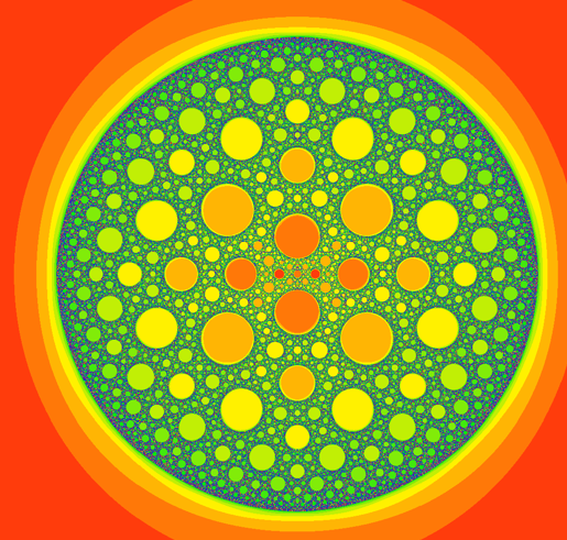
Figure 1. The Julia set of $f$.

With the spherical metric inherited from the round metric on $\widehat{\mathbb{C}}$, the Julia set $J_{f}$ becomes a metric space. As a dynamical system, the map $f$ is hyperbolic—each critical point converges to an attracting cycle—and critically finite—the orbits of the critical points are finite. Hyperbolicity is equivalent to the condition that the restriction $f\nobreak\mskip 2.0mu\mathpunct{}\nonscript\mkern-3.0mu{:}\allowbreak\mskip 6.0mu plus 1.0muJ_{f}\to J_{f}$ is an expanding self-covering map. In this setting, hyperbolicity is a dynamical regularity condition that leads to strong metric consequences. As is visually evident, $J_{f}$ is approximately-self-similar (see Definition 3.4). A key invariant of $J_{f}$ is its Hausdorff dimension $\operatorname{hdim}(J_{f})$. For carpet Julia sets, we have $1<\operatorname{hdim}(J_{f})<2$; see [PUZ89, HS01] for the lower and upper bounds, respectively. A less obvious fact (for any hyperbolic rational map) is that, with $q=\operatorname{hdim}(J_{f})$ and $\mathcal{H}^{q}$ the corresponding Hausdorff measure on $J_{f}$, then $0<\mathcal{H}^{q}(J_{f})<\infty$ [PU10, Theorem 9.1.6. Corollary 9.1.7]. In particular, for any ball $B(x,r)$ with $x\in J_{f}$, and any $r\leq\operatorname{diam}(J_{f})$we have $\mathcal{H}^{q}(B(x,r))\asymp r^{q}$, with implicit constants independent of $x$ and $r$. This latter condition is known as Ahlfors $q$-regularity.

A homeomorphism between metric spaces is quasi-symmetric if it does not distort the roundness of balls too much; see §3.3. The Ahlfors-regular conformal gauge $\mathcal{G}$ of $J_{f}$ is the set of all metric measure spaces $(X,d,\mu)$ such that there exists a quasi-symmetric homeomorphism $(J_{f},d_{Spherical})\to(X,d)$ and, for some $q>0$, the measure $\mu$ is $q$-Ahlfors regular with respect to $d$; see [Hei01, HP09]. The regularity assumption on $\mu$ implies that $\mu$ is comparable to the $q$-dimensional Hausdorff measure $\mathcal{H}^{q}$ on $X$. The Ahlfors-regular conformal dimension of $J_{f}$ is the infimum over such exponents $q$, i.e.,

$$\operatorname{ARCdim}(J_{f})\coloneqq\inf\{\operatorname{hdim}(X)\mid(X,d,\mu)\in\mathcal{G}(J_{f})\};$$

see [MT10] for an introduction. For approximately self-similar carpets $X$, such as the Julia set $J_{f}$ of Figure 1, we know $1<\operatorname{ARCdim}(X)<2$; see [Mac10]. Interest in conformal dimension stems in part from the following. Limit sets of Kleinian groups acting on the Riemann sphere and, more generally, boundaries of hyperbolic groups are another source of approximately self-similar spaces. In that setting, the conformal dimension, analogously defined, carries significant information about the group; see [Kle06].

Hyperbolicity and the critically finite property implies, by a rigidity result of W. Thurston [DH93], that the geometry and dynamics on $J_{f}$ is determined by combinatorial homotopy-theoretic data: the conjugacy-up-to-isotopy class of the map, relative to its post-critical set. More precisely: if $g$ is another rational map, and if there are orientation-preserving homeomorphisms $\phi_{0},\phi_{1}\nobreak\mskip 2.0mu\mathpunct{}\nonscript\mkern-3.0mu{:}\allowbreak\mskip 6.0mu plus 1.0mu(\widehat{\mathbb{C}},P_{f})\to(\widehat{\mathbb{C}},P_{g})$ such that $\phi_{0}\circ f=g\circ\phi_{1}$ on $P_{f}$ and $\phi_{0}$ is isotopic to $\phi_{1}$ through homeomorphisms agreeing on $P_{f}$, then we may take $\phi_{0}=\phi_{1}$ to be a Möbius transformation. Hence the invariant $\operatorname{ARCdim}(J_{f})$ is determined from combinatorial data.

For general hyperbolic critically finite rational maps with connected Julia set, our main result, Theorem A, implies an estimate for $\operatorname{ARCdim}(J_{f})$ in terms of combinatorial data. In concrete cases, by-hand computations with this data can yield nontrivial rigorous upper and lower bounds. For the carpet Julia set of Figure 1, such computations yield $1.6309\approx\frac{1}{1-\log_{6}2}\leq\operatorname{ARCdim}(J_{f})\leq\frac{2}{1-\log_{6}(10/13)}\approx 1.7445$. See §7 for details.

1.2. Combinatorial encoding

Our methods rely on a particular method of combinatorial encoding of rational maps [Thu20]. We choose a finite graph $G_{0}$, called a spine, onto which $\widehat{\mathbb{C}}-P_{f}$ deformation retracts. The homotopy type of $G_{0}$ depends only on $\#P_{f}$. Letting $G_{1}=f^{-1}(G_{0})\subset\widehat{\mathbb{C}}-P_{f}$, we obtain two graph maps $\pi,\phi\nobreak\mskip 2.0mu\mathpunct{}\nonscript\mkern-3.0mu{:}\allowbreak\mskip 6.0mu plus 1.0muG_{1}\rightrightarrows G_{0}$, where $\pi$ and $\phi$ are respectively the restrictions of $f$ and of the deformation retraction. The data $(\pi,\phi)$ is a virtual endomorphism of graphs and is well-defined up to a notion of homotopy equivalence; see [Thu20, Definition 2.2]. We denote by $[\pi,\phi]$ the homotopy class of $(\pi,\phi)$. Figure 2 illustrates the data for the above map $f$.

$$G_{1}=\vbox{\hbox{$\includegraphics[width=108.405pt]{barycenter-tri-11}$}}\qquad G_{0}=\vbox{\hbox{$\includegraphics[width=104.79128pt]{barycenter-tri-10}$}}$$

Figure 2. Spines for the map $f$, up to conjugacy-up-to-isotopy. Doubling the large Euclidean equilateral triangles over their boundaries gives two Riemann surfaces, each isomorphic to $\widehat{\mathbb{C}}$. The map $f$ sends each small triangle at left to one of the two large triangles at right and implements barycentric subdivision. The set of vertices of the large triangles is $P_{f}$. Half of a spine $G_{0}$ of $\widehat{\mathbb{C}}-P_{f}$ is shown at right, and its preimage $G_{1}$ under the piecewise-affine map homotopic to $f$ is shown at left. The map $\pi$ is the covering map preserving colors, while the map $\phi$ (defined up to homotopy) is induced by the deformation retraction.

For any iterate $n\in\mathbb{N}$, the Julia set of $f$ is the same as that of $f^{n}$. It follows from the expanding nature of the dynamics of $f$ that upon replacing $f$ by a suitable iterate, we may assume the virtual endomorphism $(\pi,\phi)$ constructed in the previous paragraph is forward expanding or, synonymously, backward contracting; see Definition 2.18. The critically finite property implies that $G_{1}$ and $G_{0}$ are connected and $\phi$ is surjective on fundamental group. This is a property we call recurrence; see Definition 2.21. To summarize: to the dynamics of a critically finite hyperbolic rational map, we associate a forward-expanding recurrent virtual graph endomorphism $(\pi,\phi)$.

It turns out (see §2) that any forward-expanding recurrent virtual graph endomorphism $(\pi,\phi)$ determines, via now-standard constructions, a dynamical system given by an expanding topological self-cover on a compact metrizable space $f\nobreak\mskip 2.0mu\mathpunct{}\nonscript\mkern-3.0mu{:}\allowbreak\mskip 6.0mu plus 1.0mu\mathcal{J}\to\mathcal{J}$ (Theorem F). The topological conjugacy class of $f$ depends only on the homotopy class $[\pi,\phi]$, suitably defined; see [IS10, Theorem 4.2].

Via other now-standard constructions, there is an associated distinguished class of Ahlfors-regular metrics $\mathcal{G}(\mathcal{J}[\pi,\phi])$ associated to $[\pi,\phi]$; see §3. If $[\pi,\phi]$ arises from a hyperbolic rational map $f$, then the spherical metric on $J_{f}$ belongs to $\mathcal{G}(\mathcal{J}[\pi,\phi])$ (Proposition 3.3).

1.3. Asymptotic $q$-conformal energies

A virtual endomorphism of graphs $(\pi,\phi)$ has, for each $q\in[1,\infty]$, an associated asymptotic $q$-conformal graph energy $\overline{E}{}^{q}(\pi,\phi)$, introduced by the second author [Thu19]. We summarize some key points; see §4 or the references for more. First, $\overline{E}{}^{q}(\pi,\phi)$ depends only on the homotopy class $[\pi,\phi]$, so that these analytic quantities depend only on combinatorial data. If $(\pi,\phi)$ arises from a rational map $f$, different choices of spine lead to homotopic graph endomorphisms, so that we may write unambiguously $\overline{E}{}^{q}(f)$. In the general case, we will also write $\overline{E}{}^{q}[\pi,\phi]$ to indicate the asymptotic energy depends only on the homotopy class. The inequality $\overline{E}{}^{\infty}[\pi,\phi]<1$ holds if and only if some iterate of $(\pi,\phi)$ is homotopic to a backward-contracting virtual graph endomorphism. If $(\pi,\phi)$ arises from a hyperbolic critically-finite rational map $f$, then $\overline{E}{}^{2}[\pi,\phi]<1$, and this property characterizes such maps among the wider class of their topological counterparts, that is, critically finite self-branched-coverings of the sphere for which each cycle in the post-critical set contains a critical point [Thu20]. As a function of $q$, the asymptotic energy $\overline{E}{}^{q}[\pi,\phi]$ is continuous and non-increasing, so that the level set $\{q\mid\overline{E}{}^{q}[\pi,\phi]=1\}$ is an interval $[q_{*}[\pi,\phi],q^{*}[\pi,\phi]]$.

1.4. Main result

Our main result relates Ahlfors-regular conformal dimension to these critical exponents, and implies that the invariant $\overline{E}{}^{q}[\pi,\phi]$ contains useful information for other values of $q$.

Theorem A.

For any recurrent, forward-expanding virtual graph endomorphism $(\pi,\phi)$,

$$q_{*}[\pi,\phi]\leq\operatorname{ARCdim}(\mathcal{J}[\pi,\phi])\leq q^{*}[\pi,\phi].$$

Equivalently, for $q=\operatorname{ARCdim}(\mathcal{J}[\pi,\phi])$, we have $\overline{E}{}^{q}[\pi,\phi]=1$.

In fact we expect that $q_{*}=q^{*}$:

Conjecture 1.1.

For any recurrent virtual graph endomorphism $[\pi,\phi]$, the function $q\mapsto\overline{E}{}^{q}[\pi,\phi]$ is either constant or strictly decreasing.

In particular if $[\pi,\phi]$ is forward-expanding then (since $\overline{E}{}^{1}[\pi,\phi]\geq 1$ and $\overline{E}{}^{\infty}[\pi,\phi]<1$), the conjecture would imply that

$$q_{*}[\pi,\phi]=q^{*}[\pi,\phi]$$

and Theorem A characterizes $\operatorname{ARCdim}$.

One might expect more to be true in Conjecture 1.1, for instance that $q\mapsto\log\overline{E}{}^{q}[\pi,\phi]$ is a convex function of $q$. More generally, it would be interesting to know the relationship between our constructions and more classical constructions in thermodynamic formalism. In this vein, we remark that Das, Przytycki, Tiozzo, and Urbański [DPT⁺19] have developed the thermodynamic formalism in a setting which includes the topologically coarse expanding conformal maps $f\nobreak\mskip 2.0mu\mathpunct{}\nonscript\mkern-3.0mu{:}\allowbreak\mskip 6.0mu plus 1.0mu\mathcal{J}\to\mathcal{J}$ considered here.

1.5. Outline

The bulk of the paper is devoted to developing the technology to prove Theorem A.

Topological dynamics

(§2) We begin with an arbitrary forward-expanding recurrent virtual endomorphism of graphs $(\pi,\phi\nobreak\mskip 2.0mu\mathpunct{}\nonscript\mkern-3.0mu{:}\allowbreak\mskip 6.0mu plus 1.0muG_{1}\rightrightarrows G_{0})$. Iteration, suitably defined, gives rise to

1. a sequence of virtual endomorphisms $(\pi^{n}_{n-1},\phi^{n}_{n-1}\nobreak\mskip 2.0mu\mathpunct{}\nonscript\mkern-3.0mu{:}\allowbreak\mskip 6.0mu plus 1.0muG_{n}\rightrightarrows G_{n-1}),n\in\mathbb{N}$;

2. a connected, locally connected, compact space $\mathcal{J}$, the inverse limit of

   $$\cdots\overset{\phi^{n+1}_{n}}{\longrightarrow}G_{n}\overset{\phi^{n}_{n-1}}{\longrightarrow}G_{n-1}\overset{\phi^{n-1}_{n-2}}{\longrightarrow}\cdots\overset{\phi^{2}_{1}}{\longrightarrow}G_{1}\overset{\phi^{1}_{0}}{\longrightarrow}G_{0};$$

3. a positively expansive self-covering map $f\nobreak\mskip 2.0mu\mathpunct{}\nonscript\mkern-3.0mu{:}\allowbreak\mskip 6.0mu plus 1.0mu\mathcal{J}\to\mathcal{J}$ of degree $d\coloneqq\deg(\pi)$;

4. the topological conjugacy class of $f\nobreak\mskip 2.0mu\mathpunct{}\nonscript\mkern-3.0mu{:}\allowbreak\mskip 6.0mu plus 1.0mu\mathcal{J}\to\mathcal{J}$ depends only on the homotopy class $[\pi,\phi]$.

Our development in this section is quite general. We consider pairs of maps $\pi,\phi\nobreak\mskip 2.0mu\mathpunct{}\nonscript\mkern-3.0mu{:}\allowbreak\mskip 6.0mu plus 1.0muX_{1}\rightrightarrows X_{0}$ between finite CW complexes equipped with length metrics and satisfying natural expansion conditions, and establish properties of the dynamics on the limit space. The main result, Theorem F, shows that under these conditions, the construction of the conformal gauges given in the next section applies.

The conformal gauge

(§3) We apply a construction in [HP09] to put a nice metric $d_{\varepsilon}$ on $\mathcal{J}$, called a visual metric. It depends on a suitably small but arbitrary parameter $\varepsilon$, and on the data of a finite cover $\mathcal{U}_{0}$ of $\mathcal{J}$ by open, connected sets. Changing this data changes the metric by a special type of quasi-symmetric map called a snowflake map. Equipped with a visual metric, $f$ is positively expansive. Even better, any ball of sufficiently small radius is sent homeomorphically and homothetically onto its image, with expansion constant $e^{\varepsilon}$. The metric space $(\mathcal{J},d_{\varepsilon},\mathcal{H}^{q})$ is Ahlfors regular of exponent $q\coloneqq\log(d)/\varepsilon=\operatorname{hdim}(\mathcal{J},d_{\varepsilon})$. Therefore, the invariant $\operatorname{ARCdim}(\mathcal{J}[\pi,\phi])$ is well-defined. See Theorem 3.2.

Energies of graph maps

(§4) When equipped with natural length metrics, the maps $\phi^{n}\coloneqq\phi^{n}_{0}\nobreak\mskip 2.0mu\mathpunct{}\nonscript\mkern-3.0mu{:}\allowbreak\mskip 6.0mu plus 1.0muG_{n}\to G_{0}$ have, for each $q\in[1,\infty]$, a $q$-conformal energy $E^{q}_{q}[\phi^{n}]$ in the sense introduced by the second author in [Thu19]. The growth rate of this energy as $n$ tends to infinity, namely $\overline{E}{}^{q}[\pi,\phi]\coloneqq\lim E^{q}_{q}[\phi^{n}]^{1/n}$, is called the asymptotic $q$-conformal energy, depends only on the homotopy class $[\pi,\phi]$, and is non-increasing in $q$ (Proposition 4.11). The expansion hypothesis implies $\overline{E}{}^{\infty}[\pi,\phi]<1$, giving the interval in the statement of Theorem A.

Combinatorial modulus

(§5) In this section we recall (and extend slightly) results on a combinatorial version of modulus in a fairly general setting, and how it is related to Ahlfors-regular conformal dimension. Although the limit space $\mathcal{J}$ hardly appears in this section, the ultimate motivation is of course to estimate its conformal dimension. In more detail, fix $n\in\mathbb{N}$. There is a natural projection $\phi^{\infty}_{n}\nobreak\mskip 2.0mu\mathpunct{}\nonscript\mkern-3.0mu{:}\allowbreak\mskip 6.0mu plus 1.0mu\mathcal{J}\to G_{n}$. The collection $\mathcal{V}_{n}$ of fibers $(\phi^{\infty}_{n})^{-1}(e)$ of closed edges $e\in E(G_{n})$ gives a covering of $\mathcal{J}$. Given a family of paths $\mathcal{C}$ in $\mathcal{J}$ and an exponent $q\geq 1$, we get a numerical invariant, $\operatorname{mod}_{q}(\mathcal{C},\mathcal{V}_{n})$, the combinatorial modulus of this family.

§§5.1–5.4 develop general properties of combinatorial modulus. We need to consider a mild generalization: we define combinatorial modulus for families of weighted curves.

§5.5 continues by relating combinatorial modulus to energies of graph maps. For this, it is technically convenient to work with the reciprocal of modulus, namely extremal length. The relation arises via the characterization of graph map energy in terms of maximum distortion of extremal length. See Theorem 4.7, which requires a formulation of extremal length in terms of weighted curves.

§5.6 recalls a result of Carrasco [Car13, Theorem 1.3], which was independently proved by Keith-Kleiner (unpublished). This result states that for a suitably self-similar space $Z$ and a suitable family of coverings $(\mathcal{S}_{n})_{n}$ indexed by $\mathbb{N}$, there is a critical exponent $q$. For a reasonably natural curve family $\Gamma$ in the space, this critical exponent distinguishes between $\operatorname{mod}_{p}(\Gamma,\mathcal{S}_{n})\to\infty$ if $p<q$ and $\operatorname{mod}_{p}(\Gamma,\mathcal{S}_{n})\to 0$ if $p>q$; see Theorem 5.11.

Sandwiching the dimension

(§6) The proof of Theorem A applies the developments in §5 and §4. We relate combinatorial modulus of curve families in the limit space to combinatorial modulus of curve families on the graphs $G_{n}$, and then to energies of graph maps.

Here is a brief summary of the proof. The collection $\{\mathcal{V}_{n}\}_{n}$ above forms a family of snapshots of the limit space, equipped with a visual metric; see §6.1. We show a curve $c\nobreak\mskip 2.0mu\mathpunct{}\nonscript\mkern-3.0mu{:}\allowbreak\mskip 6.0mu plus 1.0muC\to G_{n}$ can be approximately lifted under $\phi^{\infty}_{n}$ to a curve $c^{\prime}\nobreak\mskip 2.0mu\mathpunct{}\nonscript\mkern-3.0mu{:}\allowbreak\mskip 6.0mu plus 1.0muC\to\mathcal{J}$ such that the composition $c^{\prime\prime}\coloneqq\phi^{\infty}_{n}\circ c^{\prime}\nobreak\mskip 2.0mu\mathpunct{}\nonscript\mkern-3.0mu{:}\allowbreak\mskip 6.0mu plus 1.0muC\to G_{n}$ is homotopic to $c$, with traces of size uniformly bounded independent of $n$. This implies that combinatorial moduli for $c$ and $c^{\prime\prime}$ on $G_{n}$ are comparable to that of $c^{\prime}$ on $\mathcal{J}$ (Lemma 6.4).

With this setup, the upper bound on conformal dimension is straightforward to verify; see §6.3. The lower bound is more involved and uses in an essential way the existence of a curve $c\nobreak\mskip 2.0mu\mathpunct{}\nonscript\mkern-3.0mu{:}\allowbreak\mskip 6.0mu plus 1.0muC\to G_{n}$ which is extremal for the distortion of extremal length in the homotopy class of $\phi^{n}_{0}\nobreak\mskip 2.0mu\mathpunct{}\nonscript\mkern-3.0mu{:}\allowbreak\mskip 6.0mu plus 1.0muG_{n}\to G_{0}$. When projected to $G_{0}$, the strands of $\phi^{n}_{0}\circ c$ are very long and cross edges of $G_{0}$ many times. We decompose $c$ into a family of subcurves, each of which projects to an edge of $G_{0}$, and make the needed estimates. See §6.4.

1.6. Applications

In §7, we give several applications of our methods to the calculation of Ahlfors-regular conformal dimension in the setting of complex dynamics, using Theorem A to estimate the conformal dimension (above and below) from a forward expanding recurrent virtual graph endomorphism $(\pi,\phi)$ in the manner discussed above.

1.6.1. Techniques for estimates

Theorem A yields practical methods for estimating the Ahlfors-regular conformal dimension. If specific $\phi$ and $q$ are given with $E^{q}_{q}(\phi)<1$, the submultiplicativity of energy under composition yields $\overline{E}{}^{q}[\pi,\phi]<1$ and thus, by Theorem A, $\operatorname{ARCdim}(\mathcal{J}[\pi,\phi])<q$. Furthermore, there are bounds on how quickly $\overline{E}{}^{q}[\pi,\phi]$ can decrease as a function of $q$ [Thu20, Proposition 6.11], so if we know $\overline{E}{}^{q}[\pi,\phi]<1$, we get an upper bound on $q^{*}$ that is smaller than $q$. See Proposition 7.1.

For lower bounds, we have the following. Set $\overline{N}[\pi,\phi]=\overline{E}{}^{1}[\pi,\phi]$. This quantity has several interpretations. It is the asymptotic growth rate of the number of edge-disjoint paths in $G_{n}$ covering non-trivial loops in $G_{0}$. It is also the asymptotic growth rate of the minimum cardinality of the fibers of $\phi_{n}\nobreak\mskip 2.0mu\mathpunct{}\nonscript\mkern-3.0mu{:}\allowbreak\mskip 6.0mu plus 1.0muG_{n}\to G_{0}$. The bounds mentioned above on how fast $\overline{E}{}^{q}$ decreases as a function of $q$ yield the following.

Theorem B.

For any recurrent forward-expanding virtual graph automorphism $[\pi,\phi]$ where $\deg(\pi)=d$, we have

$$\operatorname{ARCdim}(\mathcal{J}[\pi,\phi])\geq\frac{1}{1-\log_{d}\overline{N}[\pi,\phi]}.$$

For the virtual endomorphism of $f$ from Figures 1 and 2, we find by hand that $\overline{N}(f)=2$ and $\overline{E}{}^{2}[\pi,\phi]<\sqrt{10/13}$, so $1.6309\approx\frac{1}{1-\log_{6}2}<\operatorname{ARCdim}(J_{f})<\frac{2}{1-\log_{6}(10/13)}\approx 1.7445$; see §7.2 for details.

If $f$ is a hyperbolic rational map and $[\pi,\phi]$ an associated virtual graph endomorphism, the quantity $\overline{N}(f)$ seems to be closely related to the topological and metric structure of the Julia set. For example, we show the following.

Theorem C.

Suppose $f$ is a critically finite hyperbolic rational map. If $J_{f}$ is a Sierpiński carpet, then $\overline{N}{}(f)>1$.

Examples show that the converse need not hold; see §7.1.

1.6.2. When the conformal dimension equals $1$

M. Carrasco [Car14, Theorem 1.2] gives a metric condition, uniformly well-spread cut points (UWSCP; Definition 7.15 below), on a compact doubling metric space $X$ which guarantees $\operatorname{ARCdim}(X)=1$. All hyperbolic polynomials and rational maps with “gasket-type” Julia sets satisfy the UWSCP condition. Combining his observation with our Theorem B, we obtain the following.

Theorem D.

Suppose $f$ is a hyperbolic rational map. If $J_{f}$ satisfies the UWSCP condition, then $\overline{N}(f)=1$.

We also show that Carrasco’s criterion for $\operatorname{ARCdim}=1$ is not necessary.

Proposition 1.2.

Let $R$ be the rational map obtained by mating the Douady rabbit quadratic polynomial with the basilica polynomial $z^{2}-1$. Then $\operatorname{ARCdim}(J_{R})=1$ but $J_{R}$ does not satisfy UWSCP.

This example is shown in Figure 3. More generally, applying our methods, InSung Park [Par21] has proved the following generalization: A hyperbolic critically finite rational map $f$ satisfies $\operatorname{ARCdim}(J_{f})=1$ if and only if $f$ is a crochet map, if and only if $\overline{N}{}(f)=1$. A crochet map is one in which any pair of points in the Fatou set is joined by a path which meets the Julia set in a countable set of points.

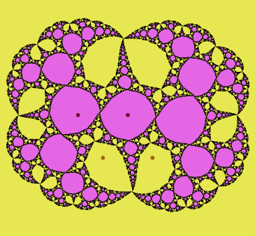
Figure 3. The mating of the rabbit (yellow) and the basilica (pink) polynomials.

1.6.3. Variation in a family

R. Devaney et al. studied the family $f_{\lambda}(z)=z^{2}+\lambda/z^{2}$ for $\lambda\in\mathbb{C}-\{0\}$ [DLU05]. Figure 4 shows the bifurcation locus in the parameter plane for this family. (The four critical points at fourth roots of $\lambda$ end up in the same orbit for this family, so analysis is simpler; see Eq. (7.7).)

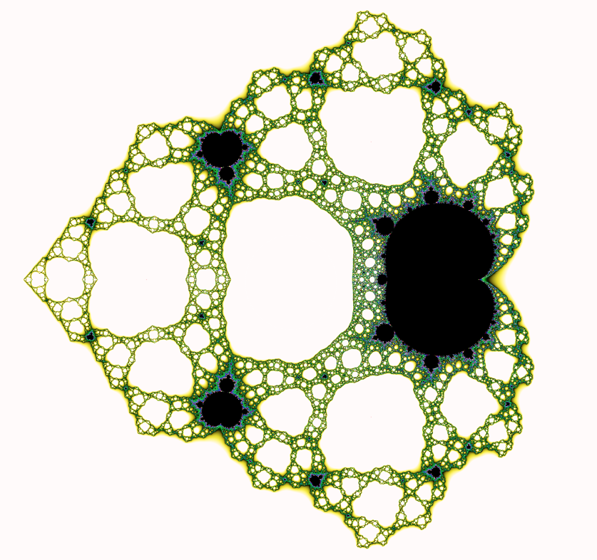
Figure 4. Parameter plane for $f_{\lambda}(z)=z^{2}+\lambda/z^{2}$. The white regions are where the $\lambda$ critical orbit escapes to the attracting fixed point at $\infty$; the small black Mandelbrot sets correspond to a renormalization, where that orbit is attracted to a different attracting cycle.

Parameters taken from the prominent “holes” along the real axis have carpet Julia sets. In §§7.3 and 7.4, we present two one-parameter families $\lambda_{n}^{\mathrm{skinny}},\lambda_{n}^{\mathrm{fat}}$, $n\in\mathbb{N}$ whose values converge to the left-most real parameter (at $\lambda=-\frac{3}{16}-\frac{\sqrt{2}}{8}$) and the origin, respectively. Figure 5 illustrates two examples.

 

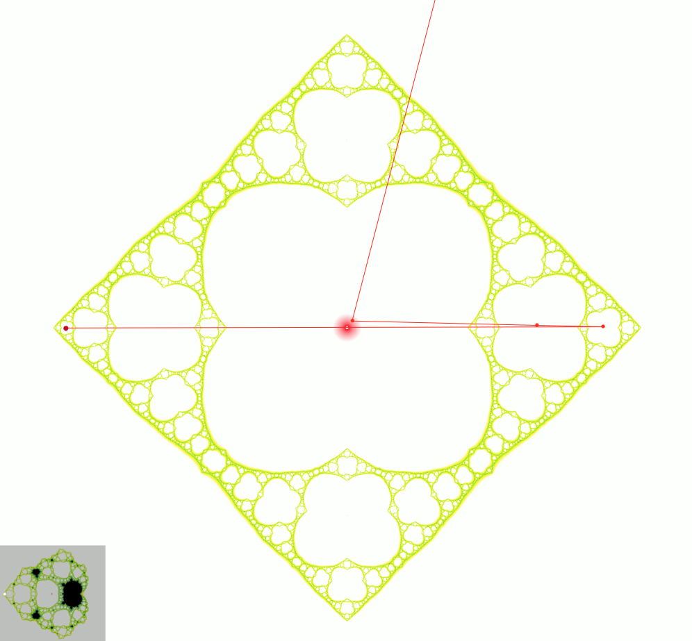
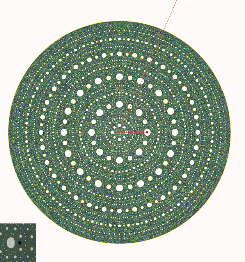
Figure 5. Two Sierpiński carpet Julia sets in the Devaney family corresponding to parameters $\lambda_{2}^{\mathrm{skinny}}\approx-.35891$ (left) and $\lambda_{2}^{\mathrm{fat}}\approx-1.4996769\times 10^{-5}$ (right). The red points are the common second iterates $x_{\lambda}$ of the finite nonzero critical points; the white points show the orbit of $x_{\lambda}$. The insets at lower left are local pictures in the parameter plane. Figures created with FractalStream [Noo].

Note the difference in the apparent “thickness” of the carpets. Though each Julia set is a Sierpiński carpet, that of $\lambda_{n}^{\mathrm{skinny}}$ visually becomes “skinnier” as $n\to\infty$, while that of $\lambda_{n}^{\mathrm{fat}}$ visually becomes “fatter” as $n\to\infty$. The former rate seems to be rather gradual, while the latter rate seems to be very fast.

Recently, M. Bonk, M. Lyubich, and S. Merenkov showed that a quasi-symmetric map between hyperbolic carpet Julia sets extends to a Möbius transformation [BLM16]. This easily implies that the three carpets shown in Figures 1 and 5 are pairwise quasi-symmetrically inequivalent. Our techniques allow us to quantify this distinction.

Theorem E.

We have

$$1<\operatorname{ARCdim}(J_{\lambda_{n}^{\mathrm{skinny}}})<1+\frac{1}{\log_{2}(2n+3)},$$

and

$$\frac{2}{1+2^{-n}}\leq\operatorname{ARCdim}(J_{\lambda_{n}^{\mathrm{fat}}})<2.$$

In particular, within this family of fixed degree, there are hyperbolic carpet maps with conformal dimension tending to 1 and to 2. This latter result answers a question of the first author and P. Haïssinsky [HP12].

1.7. Related work

Kwapisz [Kwa20] uses a similar approach to estimating the conformal dimension for Sierpiński carpets. In his paper, he considers only the standard square carpet, but uses very similar notions, with the slight variation that his $q$-resistance $r(e)$ is related to our $q$-length $\alpha(e)$ by

(1.3) $$r(e)=\alpha(e)^{q-1}.$$

(In particular, as in this paper, there are quantities associated to the edges rather than the vertices, as contrasted with the more common notions of combinatorial $q$-modulus in the literature.) With this correspondence, Kwapisz’ formulas match with ours; for instance, his $P(\mathcal{J})$ [Kwa20, Eq. (1.2)] agrees with our $\bigl{(}E^{1}_{q}(\phi)\bigr{)}^{q}$ in Eq. (4.4). One difference between our approaches is that he deals with signed flows as in electrical networks, while we deal with more general unsigned tensions related to elasticity; see the discussion in [Thu19, Appendix B].

A more substantive difference is that our $q$-conformal energies enjoy exact sub-multiplicativity [Thu19, Prop. A.12], while Kwapisz only proves weak sub-multiplicativity, up to a constant [Kwa20, Theorem 1.3]. On the other hand, by only asking for weak sub-multiplicativity, he is able to get bounds on $q$-resistance for both the graph analogous to the one we consider (his $\mathcal{G}_{n}$) and its dual. Correspondingly, he gets numerical lower bounds, in addition to numerical upper bounds analogous to the ones we get. (Our numerical lower bounds rely on Theorem B, which is unlikely to be sharp in general.)

In another direction, in the non-dynamical setting of Gromov hyperbolic complexes, Bourdon and Kleiner [BK15] consider families of analytic invariants such as $\ell^{p}$ cohomology and separation properties of certain associated function spaces. It would be interesting to know if there is a connection to this work in our setting.

Acknowledgements

We thank Caroline Davis, InSung Park, and Giulio Tiozzo for useful conversations. The first author was supported by the Simons Foundation under Grant Numbers 245269 and 615022. The second author was supported by the National Science Foundation under Grant Numbers DMS-1507244 and DMS-2110143.

2. Topological dynamics

The main result of this section is the following theorem, giving good dynamical properties of the action on a limit space.

Theorem F.

Suppose $X_{0},X_{1}$ are finite CW complexes equipped with complete length metrics. Suppose $\pi,\phi\nobreak\mskip 2.0mu\mathpunct{}\nonscript\mkern-3.0mu{:}\allowbreak\mskip 6.0mu plus 1.0muX_{1}\rightrightarrows X_{0}$ is a $\lambda$-backward-contracting and recurrent virtual endomorphism, and let $f\nobreak\mskip 2.0mu\mathpunct{}\nonscript\mkern-3.0mu{:}\allowbreak\mskip 6.0mu plus 1.0mu\mathcal{J}\to\mathcal{J}$ be the induced dynamics on its limit space. Then

1. The space $\mathcal{J}$ is connected and locally connected.

2. The map $f\nobreak\mskip 2.0mu\mathpunct{}\nonscript\mkern-3.0mu{:}\allowbreak\mskip 6.0mu plus 1.0mu\mathcal{J}\to\mathcal{J}$ is a positively expansive covering map of degree $\deg(\pi)$.

3. The dynamical system $f\nobreak\mskip 2.0mu\mathpunct{}\nonscript\mkern-3.0mu{:}\allowbreak\mskip 6.0mu plus 1.0mu\mathcal{J}\to\mathcal{J}$ is topologically coarse expanding conformal (cxc), in the sense of Haïssinsky and Pilgrim [HP09].

The terminology is defined in §2.1 and §2.5. One main result of [HP09] is that topologically cxc systems have a canonically associated nonempty set of special Ahlfors-regular metrics, called visual metrics. In §3, we will describe the geometry of $\mathcal{J}$ when equipped with such metrics.

Theorem F could be deduced as follows. Nekrashevych [Nek14, Theorem 5.10] associates to such a virtual endomorphism a self-similar recurrent contracting group action. Such an object has also an associated limit space homeomorphic to $\mathcal{J}$ that is connected and locally connected [Nek05, Theorem 3.5.1], establishing (1). Moreover, there is an induced dynamics on this limit space naturally conjugate to $f\nobreak\mskip 2.0mu\mathpunct{}\nonscript\mkern-3.0mu{:}\allowbreak\mskip 6.0mu plus 1.0mu\mathcal{J}\to\mathcal{J}$. Conclusions (2) and (3) then follow from [HP11, Theorem 6.15]. To keep this work self-contained, and because we have later need of certain other related technical facts, we give more direct arguments.

To prove Theorem F, we present the limit space as a subspace of the infinite product $(X_{1})^{\infty}$, following Ishii and Smillie [IS10]. We generalize the theory of homotopy pseudo-orbits developed there to families of homotopy pseudo-orbits parameterized by a space $A$, and show, by generalizing their results on homotopy shadowing, that such a family determines a map $A\to\mathcal{J}$ (Theorem G). We prove that the limit space is locally path-connected by applying this generalization to the case when $A=I$ is an interval (§2.6). To obtain the needed family of homotopy pseudo-orbits in this setting, we develop in §2.4 a general notion of approximate path-lifting.

For technical reasons, we need to control the geometry of non-rectifiable paths. To this end, we introduce the size of a path, defined to be the diameter of the lift to a universal cover; see §2.3. We do this mainly since we apply our development to limits of paths that need not preserve rectifiability.

We also present the associated limit space $\mathcal{J}$ in an equivalent, but more convenient, way as an inverse limit of spaces with increasingly large diameter; see Theorem G^′. To find path families, we also need to find “homotopy sections” of projections from $\mathcal{J}$ We therefore need results on homotopy shadowing and homotopy sections in those settings; see and §2.7, respectively.

2.1. Topologically cxc systems

We first recall the notion of topologically cxc systems. To streamline our presentation, we specialize the setup of [HP09] to the case of self-covers. We next define positively expansive systems. Finally, we show that conclusions (1) and (2) of Theorem F imply conclusion (3).

Suppose $\mathcal{J}$ is a compact, connected, and locally-connected topological space, and $f\nobreak\mskip 2.0mu\mathpunct{}\nonscript\mkern-3.0mu{:}\allowbreak\mskip 6.0mu plus 1.0mu\mathcal{J}\to\mathcal{J}$ is a self-covering. A finite open cover $\mathcal{U}_{0}$ of $\mathcal{J}$ by connected sets generates inductively a sequence of coverings $\mathcal{U}_{n},n\in\mathbb{N}$, via the recipe

(2.1) $$\mathcal{U}_{n+1}\coloneqq\{\widetilde{U}\mid U\in\mathcal{U}_{n},\widetilde{U}\text{ is a component of }f^{-1}(U)\}.$$

Also set

$$\mathbf{U}\coloneqq\bigcup_{n}\mathcal{U}_{n}.$$

The mesh of a covering of a metric space is the supremum of the diameters of its elements.

Definition 2.2.

The pair of the dynamical system $f\nobreak\mskip 2.0mu\mathpunct{}\nonscript\mkern-3.0mu{:}\allowbreak\mskip 6.0mu plus 1.0mu\mathcal{J}\to\mathcal{J}$ and cover $\mathcal{U}_{0}$ is said to satisfy Axiom [Expansion] if, for some (equivalently, any) metric on $\mathcal{J}$ compatible with the topology, the mesh of $\mathcal{U}_{n}$ from Eq. (2.1) tends to zero as $n\to\infty$. The map $f$ satisfies [Expansion] if there is some $\mathcal{U}_{0}$ satisfying this condition.

Lemma 2.3.

Suppose $\mathcal{J}$ is compact, connected, and locally connected, $f\nobreak\mskip 2.0mu\mathpunct{}\nonscript\mkern-3.0mu{:}\allowbreak\mskip 6.0mu plus 1.0mu\mathcal{J}\to\mathcal{J}$ is a covering map, and $\mathcal{U}_{0}$ is a covering so $(f,\mathcal{U}_{0})$ satisfies Axiom [Expansion]. Then this dynamical system satisfies the following additional two axioms:

• [Degree] For fixed $n$ there is a uniform upper bound on the cardinality of fibers of restrictions $f^{\circ n}\nobreak\mskip 2.0mu\mathpunct{}\nonscript\mkern-3.0mu{:}\allowbreak\mskip 6.0mu plus 1.0mu\widetilde{U}_{n}\to U_{0}$, for all $U_{0}\in\mathcal{U}_{0}$ and $\widetilde{U}_{n}\in\mathcal{U}_{n}$.

• [Irreducibility] For any nonempty open set $W\subset\mathcal{J}$, there is an integer $N$ for which $f^{\circ N}(W)=\mathcal{J}$.

On the conditions of this lemma, $f$ is topologically cxc. The general definition of topologically cxc is that there exists a finite open cover $\mathcal{U}_{0}$ such that all three axioms [Expansion], [Degree], and [Irreducibility] hold.

Proof.

For an self-cover satisfying axiom [Expansion], axiom [Degree] clearly holds, since for large enough $n$ the elements of $\mathcal{U}_{n}$ will be evenly covered.

To show [Irreducibility], fix arbitrarily a metric on $\mathcal{J}$ compatible with its topology. For $x\in\mathcal{J}$, define

$$Y(x) \coloneqq\{\,y\in X\mid\text{the backward orbit of $y$ accumulates at $x$}\,\}$$

$$=\{\,y\in X\mid\text{there is a sequence }\tilde{y}_{n_{k}}\in f^{-n_{k}}(y)\text{ s.t.\ }\lim_{k\to\infty}\tilde{y}_{n_{k}}=x\,\}.$$

We first claim $Y(x)$ is nonempty for each $x$. To see this, fix $x\in\mathcal{J}$, and let $y$ be any accumulation point of the forward orbit of $x$, i.e., $\lim_{k\to\infty}f^{\circ n_{k}}(x)=y$. Let $U\in\mathcal{U}_{0}$ contain $y$. For each sufficiently large $k$, let $\widetilde{U}_{n_{k}}$ be the unique component of $f^{-n_{k}}(U)$ containing $x$, and pick $\tilde{y}_{n_{k}}\in\widetilde{U}_{n_{k}}\cap f^{-n_{k}}(y)$. Then $\tilde{y}_{n_{k}}\to x$ since $\operatorname{diam}\widetilde{U}_{n_{k}}\to 0$. Hence $y\in Y(x)$.

Now suppose $y\in Y(x)$ is arbitrary and choose $U\in\mathcal{U}_{0}$ with $y\in U$. The same reasoning with $\operatorname{diam}\widetilde{U}_{n_{k}}$ shows that $U\subset Y(x)$. Since $X$ is connected and covered by $\mathcal{U}_{0}$, we conclude $Y(x)=X$. Since $x$ is arbitrary, we conclude the set of backward orbits under $f$ of each point is dense in $X$.

Now fix an arbitrary nonempty open set $W$ as in the statement of Axiom [Irreducible]. By [Expansion], there exists $U\in\mathbf{U}$ with $U\subset W$. Pick $y\in U$. By the previous paragraph, there exists a backward orbit of $y$ accumulating at $y$. Pulling back $U$ along this backward orbit, [Expansion] implies that there exists some $\widetilde{U}\in\mathbf{U}$ so that $\widetilde{U}\subset U$ and $f^{\ocirc m}\nobreak\mskip 2.0mu\mathpunct{}\nonscript\mkern-3.0mu{:}\allowbreak\mskip 6.0mu plus 1.0mu\widetilde{U}\to U$ is a covering map for some $m>0$. The previous paragraph implies $\bigcup_{n=0}^{\infty}f^{nm}(\widetilde{U})=X$. By our choice of $m$ and $\widetilde{U}$, this is an increasing union. Since $X$ is compact, $f^{nm}(\widetilde{U})=X$ for some $n$. Then $N=nm$ suffices for the statement, since $\widetilde{U}\subset W$. ∎

Definition 2.4 (Positively expansive).

Let $(\mathcal{J},d)$ be a metric space. A continuous surjection $f\nobreak\mskip 2.0mu\mathpunct{}\nonscript\mkern-3.0mu{:}\allowbreak\mskip 6.0mu plus 1.0mu\mathcal{J}\to\mathcal{J}$ is positively expansive if there is a constant $e>0$ so that for any $x\neq y\in\mathcal{J}$ there is an $n>0$ so that $d(f^{n}(x),f^{n}(y))>e$.

Note that a positively expansive map is locally injective.

In the case $\mathcal{J}$ is compact, positively expansive is equivalent to the following condition: there exists a neighborhood $N\supset\{(x,x)\nobreak\mskip 2.0mu\mathpunct{}\nonscript\mkern-3.0mu{:}\allowbreak\mskip 6.0mu plus 1.0mux\in\mathcal{J}\}$ of the diagonal such that if $x,y\in\mathcal{J}$ satisfy $(f^{i}x,f^{i}y)\in N$ for all $i\geq 0$, then $x=y$. (In particular, positively expansive is independent of the metric.) In addition, by a theorem of Reddy [AH94, Theorem 2.2.10] there exists a compatible metric $D$ on $\mathcal{J}$, called an adapted metric, and expansion constants $\delta>0$ and $0<\lambda<1$ such that for any $x,y\in\mathcal{J}$,

$$D(x,y)\leq\delta\implies D(f(x),f(y))\geq\lambda^{-1}D(x,y).$$

Note that this implies $f$ is a homeomorphism on $\delta$-balls in the $D$-metric.

Proposition 2.5 (Positively expansive implies [Expansion]).

Suppose $\mathcal{J}$ is compact and locally connected, and $f\nobreak\mskip 2.0mu\mathpunct{}\nonscript\mkern-3.0mu{:}\allowbreak\mskip 6.0mu plus 1.0mu\mathcal{J}\to\mathcal{J}$ is a positively expansive covering map. Then $f$ satisfies Axiom [Expansion].

To prove this, we will need the following result.

Theorem 2.6 (Eilenberg constants [AH94, Theorem 2.1.1]).

Let $X$ be compact and $f\nobreak\mskip 2.0mu\mathpunct{}\nonscript\mkern-3.0mu{:}\allowbreak\mskip 6.0mu plus 1.0muX\to Y$ a continuous surjective local homeomorphism. Then there exist two positive numbers $\tau$ and $\mu$ such that each subset $U$ of $Y$ with diameter less than $\tau$ determines a decomposition of the set $f^{-1}(U)=U_{1}\cup\dots\cup U_{d}$ with the following properties:

1. $f\nobreak\mskip 2.0mu\mathpunct{}\nonscript\mkern-3.0mu{:}\allowbreak\mskip 6.0mu plus 1.0muU_{i}\to U$ is a homeomorphism;

2. for $i\neq j$ no point of $U_{i}$ is closer than $2\mu$ to a point of $U_{j}$; and

3. for each $\eta>0$ there exists $0<\varepsilon<\tau$ such that $\operatorname{diam}U<\varepsilon\implies\operatorname{diam}U_{j}<\eta$ for all $j$.

Proof of Proposition 2.5.

Equip $\mathcal{J}$ with an adapted metric. We apply Theorem 2.6 with $X=Y=\mathcal{J}$ and obtain the constant $\tau$. Let $\delta$ be as in the definition of adapted metric, and take the constant $\eta$ in Theorem 2.6 so that $\eta<\delta$; we obtain a constant $\varepsilon$. In summary: any open connected set $U$ of diameter at most $\varepsilon$ is evenly covered by $f$ and has preimages $\widetilde{U}_{1},\ldots,\widetilde{U}_{d}$ of diameter at most $\delta$. The definition of adapted metric then implies that $f\nobreak\mskip 2.0mu\mathpunct{}\nonscript\mkern-3.0mu{:}\allowbreak\mskip 6.0mu plus 1.0mu\widetilde{U}_{j}\to U$ expands distances by at least the factor $\lambda^{-1}$ and so the inverse branches $f_{j}^{-1}\nobreak\mskip 2.0mu\mathpunct{}\nonscript\mkern-3.0mu{:}\allowbreak\mskip 6.0mu plus 1.0muU\to\widetilde{U}_{j}$ contract distances by at least the factor $\lambda$.

Since $\mathcal{J}$ is locally connected and compact, there is a finite open cover $\mathcal{U}_{0}$ by connected sets such that each element has diameter at most $\varepsilon$. The previous paragraph implies that the covering $\mathcal{U}_{1}$ has mesh at most $\lambda\varepsilon<\varepsilon$. Induction shows $\mathrm{mesh}(\mathcal{U}_{n})<\lambda^{n}\varepsilon\to 0$ as required in Axiom [Expansion]. ∎

2.2. Length spaces

In this subsection, we prepare for the proof of local connectivity by collecting some technical results related to covering maps and length spaces. Here, $X$ denotes a finite, hence compact, connected CW complex, equipped with a compatible length metric. The Hopf-Rinow theorem implies that $X$ is a geodesic metric space. While balls might not be simply-connected, they are path-connected. The systole is the length of the shortest essential loop, i.e.,

$$\operatorname{systole}(X)\coloneqq\inf\{\ell(\gamma)\mid[\gamma]\neq 1,[\gamma]\in\pi_{1}(X)\}.$$

This is positive, since $X$ is compact. Since $X$ is a length space, any cover $\widetilde{X}$ inherits a lifted metric by lengths of paths. Balls of radius less than $\tfrac{1}{2}\operatorname{systole}(X)$ are simply-connected and thus evenly covered.

Lemma 2.7.

Let $X$ be a finite connected CW complex with a length metric. Suppose $p\nobreak\mskip 2.0mu\mathpunct{}\nonscript\mkern-3.0mu{:}\allowbreak\mskip 6.0mu plus 1.0mu\widetilde{X}\to X$ is a covering map, $\widetilde{X}$ is equipped with the lifted metric, and $r<\tfrac{1}{4}\operatorname{systole}(X)$. Then for any $\tilde{x}\in\widetilde{X}$ with $p(\tilde{x})=x$, the restriction $p\nobreak\mskip 2.0mu\mathpunct{}\nonscript\mkern-3.0mu{:}\allowbreak\mskip 6.0mu plus 1.0muB(\tilde{x},r)\to B(x,r)$ is an isometry.

This is standard, but we provide a proof for completeness.

Proof.

The definition of the metric on $\widetilde{X}$ implies that $p$ preserves the length of paths, and is therefore 1-Lipschitz. Thus $p(B(\tilde{x},r))\subset B(x,r)$. We have $p(B(\tilde{x},r))=B(x,r)$ since a geodesic joining $x$ to $y\in B(x,r)$ lifts to a path of the same length joining $\tilde{x}$ to some point $\tilde{y}$ which therefore lies in $B(\tilde{x},r)$. We now claim that $p\nobreak\mskip 2.0mu\mathpunct{}\nonscript\mkern-3.0mu{:}\allowbreak\mskip 6.0mu plus 1.0muB(\tilde{x},r)\to B(x,r)$ is an isometry. Suppose $\tilde{a},\tilde{b}\in B(\tilde{x},r)$, and put $a=p(\tilde{a})$ and $b=p(\tilde{b})$. Then $a,b\in B(x,r)$. Consider the piecewise geodesic path $\gamma$ comprised of 3 length-minimizing segments which runs from $x$ to $a$, then from $a$ to $b$, then from $b$ to $x$. This loop may not lie in $B(x,r)$. However, $\ell(\gamma)<4r$ and both endpoints are at $x$, so $\gamma\subset B(x,2r)$, which is evenly covered by the choice of $r$. It follows that the middle segment lifts to a segment joining $\tilde{a}$ to $\tilde{b}$ of length equal to $d(a,b)$. Hence $d(\tilde{a},\tilde{b})\leq d(a,b)$ and the result is proved. ∎

If $\phi\nobreak\mskip 2.0mu\mathpunct{}\nonscript\mkern-3.0mu{:}\allowbreak\mskip 6.0mu plus 1.0muX\to Y$ is a map between metric spaces, we say a non-decreasing function $\omega_{\phi}\nobreak\mskip 2.0mu\mathpunct{}\nonscript\mkern-3.0mu{:}\allowbreak\mskip 6.0mu plus 1.0mu[0,\operatorname{diam}(X)]\to[0,\operatorname{diam}(Y)]$ is a modulus of continuity if, for all $E\subset X$, $\operatorname{diam}\phi(E)\leq\omega_{\phi}(\operatorname{diam}E)$.

Lemma 2.8.

Suppose $X,Y$ are compact, connected, CW complexes equipped with length metrics, and $\phi\nobreak\mskip 2.0mu\mathpunct{}\nonscript\mkern-3.0mu{:}\allowbreak\mskip 6.0mu plus 1.0muX\to Y$ is a continuous map, with modulus of continuity $\omega_{\phi}$. Let $p_{Y}\nobreak\mskip 2.0mu\mathpunct{}\nonscript\mkern-3.0mu{:}\allowbreak\mskip 6.0mu plus 1.0mu\widetilde{Y}\to Y$ be any covering map, and equip $\widetilde{Y}$ with the lifted metric. Let $p_{X}\nobreak\mskip 2.0mu\mathpunct{}\nonscript\mkern-3.0mu{:}\allowbreak\mskip 6.0mu plus 1.0mu\widetilde{X}\to X$ and $\widetilde{\phi}\nobreak\mskip 2.0mu\mathpunct{}\nonscript\mkern-3.0mu{:}\allowbreak\mskip 6.0mu plus 1.0mu\widetilde{X}\to\widetilde{Y}$ be the maps induced by pullback, and equip $\widetilde{X}$ with the lifted metric from $X$. Then $\widetilde{\phi}$ is uniformly continuous, with modulus of continuity $\omega_{\widetilde{\phi}}$ independent of the cover $p_{Y}$. Indeed, there exists $r_{0}>0$ depending only on $\phi\nobreak\mskip 2.0mu\mathpunct{}\nonscript\mkern-3.0mu{:}\allowbreak\mskip 6.0mu plus 1.0muX\to Y$ so that we can take

$$\omega_{\widetilde{\phi}}=\begin{cases}\omega_{\phi}(\delta)&\delta\leq r_{0}\\ \omega_{\phi}(r_{0})+\omega_{\phi}(r_{0})\delta/r_{0}&\delta>r_{0}.\end{cases}$$

So $\widetilde{\phi}$ behaves just like $\phi$ at small scales, and is Lipschitz at large scales.

Proof.

Put $s_{0}\coloneqq\frac{1}{4}\operatorname{systole}(Y)$. By the uniform continuity of $\phi$, there exists $0<r_{0}<\frac{1}{4}\operatorname{systole}(X)$ such that for each $x\in X$ and $y=\phi(x)$, we have $\phi(B(x,r_{0}))\subset B(y,s_{0})$. Fix now $\tilde{x}\in\widetilde{X}$ and put $x=p_{X}(\tilde{x})$, $\tilde{y}=\widetilde{\phi}(\tilde{x})$, and $y=p_{Y}(\tilde{y})=\phi(x)$. By Lemma 2.7,

$$p_{Y}^{-1}\nobreak\mskip 2.0mu\mathpunct{}\nonscript\mkern-3.0mu{:}\allowbreak\mskip 6.0mu plus 1.0muB(y,s_{0})\to B(\tilde{y},s_{0})$$

and

$$p_{X}\nobreak\mskip 2.0mu\mathpunct{}\nonscript\mkern-3.0mu{:}\allowbreak\mskip 6.0mu plus 1.0muB(\tilde{x},r_{0})\to B(x,r_{0})$$

are isometric homeomorphisms. Now fix $0<r\leq r_{0}$. Then

$$\widetilde{\phi}(B(\tilde{x},r))=(p_{Y}^{-1}\circ\phi\circ p_{X})(B(\tilde{x},r))=p_{Y}^{-1}(\phi(B(x,r))\subset p_{Y}^{-1}(B(y,\omega_{\phi}(r)))\subset B(\tilde{y},\omega_{\phi}(r)),$$

establishing the estimate in the case $\delta\leq r_{0}$. For the other case, suppose $a,b\in\widetilde{Y}$ are at distance $R\geq r_{0}$, and let $\gamma$ be a geodesic joining $a$ to $b$. Divide $\gamma$ into sub-segments $\gamma=\gamma_{0}*\gamma_{1}*\ldots*\gamma_{n}$ with $\ell(\gamma_{0})\leq r_{0}$ and $\ell(\gamma_{i})=r_{0}$ for $i=1,\ldots,n$, so that $nr_{0}\leq\ell(\gamma)\leq(n+1)r_{0}$. Then

$$d(\widetilde{\phi}(a),\widetilde{\phi}(b)) \leq\sum_{i=0}^{n}\operatorname{diam}\phi(\gamma_{i})\leq\omega_{\phi}(r_{0})+\omega_{\phi}(r_{0})d(a,b)/r_{0}.\qed$$

2.3. Sizes of paths and traces of homotopies

It would be nice to always work with the length of paths, but it turns out that not all the paths we consider are rectifiable. (In particular, we consider paths in the Julia set $\mathcal{J}$ and their projections to the finite approximations $G_{n}$; these projections are usually not rectifiable.) We could consider the diameter of paths, but we also need to lift paths to covers. We work instead with a hybrid.

Convention 2.9.

For paths $\gamma\nobreak\mskip 2.0mu\mathpunct{}\nonscript\mkern-3.0mu{:}\allowbreak\mskip 6.0mu plus 1.0muI\to X$, the path $\overline{\gamma}$ is the reversed path, and $\gamma_{1}*\gamma_{2}$ denotes composition of paths, defined when $\gamma_{1}(1)=\gamma_{2}(0)$. For homotopies $H\nobreak\mskip 2.0mu\mathpunct{}\nonscript\mkern-3.0mu{:}\allowbreak\mskip 6.0mu plus 1.0muI\times A\to X$, we will more generally use the same notations $\overline{H}$ and $H_{1}*H_{2}$, always operating on the first input (which is an interval).

Definition 2.10.

For $X$ a locally simply-connected length space, $A$ a simply-connected auxiliary space (usually the interval), and $\gamma\nobreak\mskip 2.0mu\mathpunct{}\nonscript\mkern-3.0mu{:}\allowbreak\mskip 6.0mu plus 1.0muA\to X$ a continuous map, there are lifts $\widetilde{\gamma}\nobreak\mskip 2.0mu\mathpunct{}\nonscript\mkern-3.0mu{:}\allowbreak\mskip 6.0mu plus 1.0muA\to\widetilde{X}$ of $\gamma$ to the universal cover of $X$. The size of $\gamma$ is the diameter of $\widetilde{\gamma}$ with respect to the lifted metric on $\widetilde{X}$:

$$\operatorname{size}(\gamma)\coloneqq\max_{s,t\in I}d_{\widetilde{X}}(\widetilde{\gamma}(s),\widetilde{\gamma}(t)).$$

The proof of the following lemma is straightforward.

Lemma 2.11 (Properties of size for paths).

The notion of size for paths (with $A$ the interval) satisfies the following properties.

1. Well-defined: $\operatorname{size}(\gamma)$ is independent of which lift of $\gamma$ to $\widetilde{X}$ you take.

2. Bounded by length: when $\gamma\nobreak\mskip 2.0mu\mathpunct{}\nonscript\mkern-3.0mu{:}\allowbreak\mskip 6.0mu plus 1.0muI\to X$ is rectifiable, $\operatorname{size}(\gamma)\leq\ell(\gamma)$.

3. Invariance under lifts: if $p\nobreak\mskip 2.0mu\mathpunct{}\nonscript\mkern-3.0mu{:}\allowbreak\mskip 6.0mu plus 1.0muX\to Y$ is a covering map, $Y$ is a length space, $X$ is equipped with the lifted metric, $\gamma\nobreak\mskip 2.0mu\mathpunct{}\nonscript\mkern-3.0mu{:}\allowbreak\mskip 6.0mu plus 1.0muI\to Y$ is a path, and $\widetilde{\gamma}\nobreak\mskip 2.0mu\mathpunct{}\nonscript\mkern-3.0mu{:}\allowbreak\mskip 6.0mu plus 1.0muI\to X$ is a lift of $\gamma$ under $p$, then $\operatorname{size}(\widetilde{\gamma})=\operatorname{size}(\gamma)$.

4. Sub-additive under path composition: $\operatorname{size}(\gamma_{1}*\gamma_{2})\leq\operatorname{size}(\gamma_{1})+\operatorname{size}(\gamma_{2})$.

5. Shortening: If $f\nobreak\mskip 2.0mu\mathpunct{}\nonscript\mkern-3.0mu{:}\allowbreak\mskip 6.0mu plus 1.0muX\to Y$ is $\lambda$-Lipschitz and $\gamma\nobreak\mskip 2.0mu\mathpunct{}\nonscript\mkern-3.0mu{:}\allowbreak\mskip 6.0mu plus 1.0muI\to X$ is a path in $X$, then $\operatorname{size}(f\circ\gamma)\leq\lambda\cdot\operatorname{size}(\gamma)$.

As a result of point (1), we will prefer to give statements with hypotheses on the size of paths and construct paths with bounds on length, even if we don’t necessarily need the length bounds for our applications.

Another central feature of our development is the following.

Definition 2.12.

For $X$ a locally simply-connected length space, $A$ an auxiliary space, and $H\nobreak\mskip 2.0mu\mathpunct{}\nonscript\mkern-3.0mu{:}\allowbreak\mskip 6.0mu plus 1.0muI\times A\to X$ a homotopy of maps from $A$ to $X$, a trace of $H$ is a path of the form $t\mapsto H(t,a)$ for fixed $a\in A$. The trace size of $H$ is the maximum size of a trace:

$$\operatorname{tracesize}(H)\coloneqq\sup_{a\in A}\,\operatorname{size}(H(\cdot,a)).$$

If two maps $f,g\nobreak\mskip 2.0mu\mathpunct{}\nonscript\mkern-3.0mu{:}\allowbreak\mskip 6.0mu plus 1.0muA\to X$ are homotopic by a homotopy of trace size at most $K$, then we write $f\sim_{K}g$.

For a homotopy $H\nobreak\mskip 2.0mu\mathpunct{}\nonscript\mkern-3.0mu{:}\allowbreak\mskip 6.0mu plus 1.0muI\times I\to X$ between two paths $\gamma_{0}$ and $\gamma_{1}$, be careful to distinguish between its size and trace size. For instance, if $H$ has bounded size, then the $\gamma_{i}$ must also have bounded size, while two paths that are very long can still have a homotopy of bounded trace size.

The trace size of a homotopy between two paths is sensitive to the parameterization of the domain of the two paths, which in turn is sensitive to details like exactly how one defines the concatenation operation on paths. We will specify the parameterization when necessary.

One thing to note now is that, if $\beta$ is a path of size $R$ and any $\varepsilon>0$, then, for any concatenatable $\gamma_{1},\gamma_{2}$ and suitable parameterization of the domain,

$$\gamma_{1}*\beta*\overline{\beta}*\gamma_{2}\sim_{R+\varepsilon}\gamma_{1}*\gamma_{2}.$$

(The parameterization to make this work uses a very small interval in the domain for $\beta*\overline{\beta}$ on the left hand side.)

Lemma 2.13.

Suppose $X,Y,Z$ are length spaces. If $f\nobreak\mskip 2.0mu\mathpunct{}\nonscript\mkern-3.0mu{:}\allowbreak\mskip 6.0mu plus 1.0muX\to Y$ and $g_{0},g_{1}\nobreak\mskip 2.0mu\mathpunct{}\nonscript\mkern-3.0mu{:}\allowbreak\mskip 6.0mu plus 1.0muY\to Z$ are maps with $g_{0}\sim_{K}g_{1}$ via the homotopy $\alpha\nobreak\mskip 2.0mu\mathpunct{}\nonscript\mkern-3.0mu{:}\allowbreak\mskip 6.0mu plus 1.0muI\times Y\to Z$, then $g_{0}\circ f\sim_{K}g_{1}\circ f$ via the homotopy $f^{*}\alpha\nobreak\mskip 2.0mu\mathpunct{}\nonscript\mkern-3.0mu{:}\allowbreak\mskip 6.0mu plus 1.0muI\times X\to Z$ given by $(t,x)\mapsto\alpha(t,f(x))$.

Proof.

The only non-trivial point is the bound on the trace size, which follows since every trace of $f^{*}\alpha$ is a trace of $\alpha$. ∎

2.4. Approximate path-lifting

Suppose $X$, $Y$, and $A$ are topological spaces, and suppose we are given maps $\phi\nobreak\mskip 2.0mu\mathpunct{}\nonscript\mkern-3.0mu{:}\allowbreak\mskip 6.0mu plus 1.0muX\to Y$ and $g\nobreak\mskip 2.0mu\mathpunct{}\nonscript\mkern-3.0mu{:}\allowbreak\mskip 6.0mu plus 1.0muA\to Y$. An approximate lift of $g$ under $\phi$ with constant $K$ is a map $g^{\prime}\nobreak\mskip 2.0mu\mathpunct{}\nonscript\mkern-3.0mu{:}\allowbreak\mskip 6.0mu plus 1.0muA\to X$ such that $\phi\circ g^{\prime}\sim_{K}g$.

Now suppose further that $X,Y$ are finite connected CW complexes, equipped with complete length metrics, and $\phi\nobreak\mskip 2.0mu\mathpunct{}\nonscript\mkern-3.0mu{:}\allowbreak\mskip 6.0mu plus 1.0muX\to Y$ is continuous and surjective on fundamental group. We consider the problem of approximately lifting paths in $Y$ under $\phi$ to paths in $X$.

In this subsection, the constants appearing in the conclusions depend on $\phi\nobreak\mskip 2.0mu\mathpunct{}\nonscript\mkern-3.0mu{:}\allowbreak\mskip 6.0mu plus 1.0muX\to Y$ and on the other constants appearing in the statements. We suppress their dependence on $\phi$.

Proposition 2.14 (Controlled approximate path-lifting).

Suppose $X$ and $Y$ are finite connected CW complexes, $\phi\nobreak\mskip 2.0mu\mathpunct{}\nonscript\mkern-3.0mu{:}\allowbreak\mskip 6.0mu plus 1.0muX\to Y$ is continuous, and $\phi_{*}\nobreak\mskip 2.0mu\mathpunct{}\nonscript\mkern-3.0mu{:}\allowbreak\mskip 6.0mu plus 1.0mu\pi_{1}(X)\to\pi_{1}(Y)$ is surjective. Then there exist a positive constant $K$ so that for any path $\gamma\nobreak\mskip 2.0mu\mathpunct{}\nonscript\mkern-3.0mu{:}\allowbreak\mskip 6.0mu plus 1.0muI\to Y$ joining endpoints $y_{0}$ to $y_{1}$, and any preimages $x_{i}\in\phi^{-1}(y_{i})$ for $i=0,1$ of these endpoints, there exists an approximate lift $\gamma^{\prime}\nobreak\mskip 2.0mu\mathpunct{}\nonscript\mkern-3.0mu{:}\allowbreak\mskip 6.0mu plus 1.0muI\to X$ with $\gamma^{\prime}(i)=x_{i}$ for $i=0,1$ with homotopy $H\nobreak\mskip 2.0mu\mathpunct{}\nonscript\mkern-3.0mu{:}\allowbreak\mskip 6.0mu plus 1.0muI\times I\to Y$ of trace size $K$. Concretely,

• $H(0,t)=\gamma(t)$ and $H(1,t)=\phi\circ\gamma^{\prime}(t)$ for $0\leq t\leq 1$;

• $H(s,i)=y_{i}$ for $i=0,1$ and $0\leq s\leq 1$; and

• $\operatorname{size}(s\mapsto H(s,t))\leq K$ for each $t\in[0,1]$.

There exist constants $C_{0}$ and $C_{1}$ so that if $\gamma$ is rectifiable, then so is $\gamma^{\prime}$, and $\ell(\gamma^{\prime})<C_{0}+C_{1}\ell(\gamma)$.

Figure 6. Approximate path lifting. The traces of the homotopies are the red lines on the right; these must be of bounded size.

In other words, approximate lifting increases lengths by controlled amounts, and the failure of a path to lift is measured by a homotopy whose traces are uniformly bounded in size, independent of the path $\gamma$; see Figure 6. (We do not use the fact that lengths are increased by controlled amounts in this paper, but it helps add motivation.) We will also say that $\phi\nobreak\mskip 2.0mu\mathpunct{}\nonscript\mkern-3.0mu{:}\allowbreak\mskip 6.0mu plus 1.0muX\to Y$ satisfies the $K$-APL condition.

Before proving the general statement, we first prove it for loops $\gamma$ of bounded length.

Lemma 2.15 (Controlled approximate loop-lifting).

In the setup of Proposition 2.14, fix $C>0$. Then there exist constants $L$ and $K$ with the following property. For any $x\in X$, $y=\phi(x)$, and loop $\lambda\nobreak\mskip 2.0mu\mathpunct{}\nonscript\mkern-3.0mu{:}\allowbreak\mskip 6.0mu plus 1.0muI\to Y$ loop based at $y$ with $\operatorname{size}(\lambda)\leq C$, there is a rectifiable loop $\lambda^{\prime}\nobreak\mskip 2.0mu\mathpunct{}\nonscript\mkern-3.0mu{:}\allowbreak\mskip 6.0mu plus 1.0muI\to X$ based at $x$ with $\ell(\lambda^{\prime})<L$ so that $\phi\circ\lambda^{\prime}\sim_{K}\lambda$.

Proof.

First fix $x\in X$ and $y=\phi(x)$. The length metrics on $X$ and $Y$ induce norms on the fundamental groups $\pi_{1}(X,x)$ and $\pi_{1}(Y,y)$. Since $\operatorname{size}(\lambda)\leq C$, the norm of $[\lambda]$ is also bounded by $C$. Since $\phi_{*}\nobreak\mskip 2.0mu\mathpunct{}\nonscript\mkern-3.0mu{:}\allowbreak\mskip 6.0mu plus 1.0mu\pi_{1}(X,x)\to\pi_{1}(Y,y)$ is surjective, there exists $L(x)$ such that the image of the ball of radius $L(x)$ in $\pi_{1}(X,x)$ contains the ball of radius $C$ in $\pi_{1}(Y,y)$. Now vary $x\in X$. By compactness, $\sup_{x\in X}L(x)$ is finite; call this $L$. Thus there exists a loop $\lambda^{\prime}$ based at $x$ of length at most $L$ for which $\phi\circ\lambda^{\prime}\sim\lambda$.

We must bound the trace size of the homotopy; in fact we bound its size. For any $\lambda$ and $\lambda^{\prime}$ as above, we can lift $\phi\circ\lambda^{\prime}$ and $\lambda$ to paths in the universal cover $\widetilde{Y}$. Fix lifts $\widetilde{\phi\circ\lambda^{\prime}}$ and $\widetilde{\lambda}$, respectively, joining common endpoints. The concatenation $\widetilde{\alpha}\coloneqq\widetilde{\phi\circ\lambda^{\prime}}*\overline{\widetilde{\lambda}}$ is a loop in the simply-connected length CW complex $\widetilde{Y}$. By Lemma 2.8 we have

$$\operatorname{diam}(\widetilde{\alpha})\leq\operatorname{diam}(\widetilde{\phi\circ\lambda^{\prime}})+\operatorname{diam}(\widetilde{\lambda})\leq\omega_{\widetilde{\phi}}(L)+C\eqqcolon D_{1}.$$

By [DK18, Lemma 9.51], $\widetilde{Y}$ is uniformly simply-connected. This implies that $\widetilde{\alpha}$ is homotopic to a constant map via a homotopy whose image has diameter $K\coloneqq K(D_{1})$, as desired. ∎

Proof of Proposition 2.14.

Pick (arbitrarily) a basepoint $x_{*}\in X$, set $y_{*}\coloneqq\phi(x_{*})$, and pick an arbitrary constant $C>0$. Divide $\gamma$ into sub-paths

$$\gamma=\gamma_{0}*\dots*\gamma_{n-1}$$

with $\operatorname{size}(\gamma_{i})\leq C$. Let the endpoints of $\gamma_{i}$ be $z_{i},z_{i+1}\in Y$, and for each $i$ pick a path $\rho_{i}$ from $y_{*}$ to $z_{i}$, of length less than $\operatorname{diam}(Y)$. Pick also paths $\rho_{0}^{\prime},\rho_{n}^{\prime}$ from $x_{*}$ to $x_{0},x_{1}$, respectively, of length less than $\operatorname{diam}(X)$. Then $\lambda_{i}\coloneqq\rho_{i}*\gamma_{i}*\overline{\rho_{i+1}}$ is a loop based at $y_{*}$ of size less then $2\operatorname{diam}(X)+C$. By Lemma 2.15, there are constants $L_{1},K_{1}$ so that, for each $i$, there is a loop $\lambda_{i}^{\prime}$ in $X$ based at $x_{*}$ with $\ell(\lambda_{i}^{\prime})<L_{1}$ and $\phi\circ\lambda_{i}^{\prime}\sim_{K_{1}}\lambda_{i}$. In addition, $\sigma_{0}\coloneqq(\phi\circ\rho_{0}^{\prime})*\overline{\rho_{0}}$ is a loop of size less than $\omega_{\widetilde{\phi}}(\operatorname{diam}Y)+\operatorname{diam}X$, so there are constants $L_{2},K_{2}$ and a loop $\sigma_{0}^{\prime}$ based at $x_{*}$ of length less than $L_{2}$ so that $\phi\circ\sigma_{0}^{\prime}\sim_{K_{2}}\sigma_{0}$. Similarly pick an approximate lift $\sigma_{n}^{\prime}$ of $\sigma_{n}\coloneqq\rho_{n}*\overline{(\phi\circ\rho_{n}^{\prime})}$. Now set

$$K \coloneqq\max(K_{1},K_{2})$$

$$D \coloneqq\max(\operatorname{diam}(X),\omega_{\widetilde{\phi}}(\operatorname{diam}(Y))$$

$$\gamma^{\prime} \coloneqq\overline{\rho^{\prime}_{0}}*\sigma_{0}^{\prime}*\lambda_{1}^{\prime}*\lambda_{2}^{\prime}*\dots*\lambda_{n-1}^{\prime}*\sigma_{n}^{\prime}*\rho^{\prime}_{n}$$

(with suitable parameterization of the domain for $\gamma^{\prime}$), so that

$$\phi\circ\gamma^{\prime} \sim_{K}\overline{(\phi\circ\rho_{0}^{\prime})}*\sigma_{0}*\lambda_{1}*\lambda_{2}*\dots*\lambda_{n-1}*\sigma_{n}*(\phi\circ\rho_{n}^{\prime})$$

$$\sim_{D+\varepsilon}\gamma_{0}*\gamma_{1}*\dots*\gamma_{n-1}=\gamma,$$

as desired.

To get the bounds on length in the case that $\gamma$ is rectifiable, choose the initial decomposition of $\gamma$ into sub-paths $\gamma_{i}$ so that, for $i>0$, $\ell(\gamma_{i})\geq C$; then we have $n\leq 1+\ell(\gamma)/C$. We can choose the paths $\lambda_{i}^{\prime}$, $\rho_{i}^{\prime}$, and $\sigma_{i}^{\prime}$ all to have length bounded by a constant, which then gives the desired bound on $\ell(\gamma)$. ∎

Remark 2.16.

Lemma 2.15 gives a bound on the overall size of the homotopy, but Proposition 2.14 only gives a bound on the trace sizes.

2.5. Multi-valued dynamical systems

We turn our attention back to dynamics. We think of two spaces and a pair of maps between them, $\pi,\phi\nobreak\mskip 2.0mu\mathpunct{}\nonscript\mkern-3.0mu{:}\allowbreak\mskip 6.0mu plus 1.0muX_{1}\rightrightarrows X_{0}$, as a multi-valued dynamical system. We introduce an associated limit space and describe it in two different ways, as in [IS10], but adopting slightly different notation. Here is how to translate between their (IS) and our (PT) notation:

$$X^{i}_{IS} =X_{i,PT};$$

$$(\iota,\sigma)_{IS}=(\iota,f)_{IS} =(\phi,\pi)_{PT};$$

$$X^{+\infty}_{IS} =\mathcal{J}_{PT}.$$

(There are also minor differences in the indexing.)

Suppose $X_{1}$ and $X_{0}$ are compact topological spaces and $\pi,\phi\nobreak\mskip 2.0mu\mathpunct{}\nonscript\mkern-3.0mu{:}\allowbreak\mskip 6.0mu plus 1.0muX_{1}\rightrightarrows X_{0}$ are two continuous maps. An orbit is a sequence of points $x_{i}\in X_{1}$ with $\pi(x_{i})=\phi(x_{i+1})$ when both sides are defined. If $x_{i}$ is defined for $1\leq i\leq n$ for some $n\geq 1$, we get the space $X_{n}$ of orbits of length $n$. If $x_{i}$ is defined for all $1\leq i$, we get the limit space $\mathcal{J}\subset X_{1}^{\mathbb{N}}$ of one-sided infinite orbits $(x_{0},x_{1},\ldots)$. Note the typographical distinction between the abstract limit space $\mathcal{J}$ of a virtual endomorphism and the concrete limit space $J_{R}\subset\widehat{\mathbb{C}}$ of a rational map $R$.

With this setup, there are two families of canonical maps

$$\phi^{n+1}_{n},\pi^{n+1}_{n}\nobreak\mskip 2.0mu\mathpunct{}\nonscript\mkern-3.0mu{:}\allowbreak\mskip 6.0mu plus 1.0muX_{n+1} \to X_{n},$$

$$\phi^{n+1}_{n}(x_{1},x_{2},\ldots,x_{n},x_{n+1}) \coloneqq(x_{1},x_{2},\ldots,x_{n})$$

$$\pi^{n+1}_{n}(x_{1},x_{2},\ldots,x_{n},x_{n+1}) \coloneqq(x_{2},\ldots,x_{n},x_{n+1}).$$

We also set $\phi^{1}_{0}\coloneqq\phi$ and $\pi^{1}_{0}\coloneqq\pi$. We can compose these to get maps $\phi^{n}_{k},\pi^{n}_{k}\nobreak\mskip 2.0mu\mathpunct{}\nonscript\mkern-3.0mu{:}\allowbreak\mskip 6.0mu plus 1.0muX_{n}\to X_{k}$ for $0\leq k\leq n$.

Convention 2.17.

Our indexing convention is such that the index of the domain appears as a superscript and index of the codomain appears as a subscript. This way, composition corresponds to “contraction” of indices, as is conventional in tensor notation.

We can present the space $\mathcal{J}$ as an inverse limit of the sequence $\phi^{n+1}_{n}$:

where the $\phi^{\infty}_{n}\nobreak\mskip 2.0mu\mathpunct{}\nonscript\mkern-3.0mu{:}\allowbreak\mskip 6.0mu plus 1.0mu\mathcal{J}\to X_{n}$ are analogues of $\phi^{n}_{k}$:

$$\phi^{\infty}_{n}(x_{1},x_{2},\dots)\coloneqq(x_{1},x_{2},\dots,x_{n}).$$

There is also a canonical map $f\nobreak\mskip 2.0mu\mathpunct{}\nonscript\mkern-3.0mu{:}\allowbreak\mskip 6.0mu plus 1.0mu\mathcal{J}\to\mathcal{J}$ induced by the one-sided shift, a kind of analogue of $\pi^{n+1}_{n}$:

$$f(x_{1},x_{2},\ldots)\coloneqq(x_{2},\ldots).$$

There are two natural modifications of a pair of maps $(\pi,\phi)$: we can iterate it, replacing the pair by

$$\pi^{n}_{0},\phi^{n}_{0}\nobreak\mskip 2.0mu\mathpunct{}\nonscript\mkern-3.0mu{:}\allowbreak\mskip 6.0mu plus 1.0muX_{n}\rightrightarrows X_{0},$$

or we can reindex, replacing the pair by

$$\pi^{n}_{n-1},\phi^{n}_{n-1}\nobreak\mskip 2.0mu\mathpunct{}\nonscript\mkern-3.0mu{:}\allowbreak\mskip 6.0mu plus 1.0muX_{n}\rightrightarrows X_{n-1}.$$

Neither of these operations changes the limit space $\mathcal{J}$, but iterating replaces the dynamics of $f$ on $\mathcal{J}$ by $f^{n}$, while reindexing does not change $f$.

We now restrict attention to expanding systems, as in [IS10], but adopting terminology of Nekrashevych [Nek14] and the second author [Thu20]. We continue with some definitions.

Definition 2.18.

Virtual endomorphisms. A pair of continuous maps $\pi,\phi\nobreak\mskip 2.0mu\mathpunct{}\nonscript\mkern-3.0mu{:}\allowbreak\mskip 6.0mu plus 1.0muX_{1}\rightrightarrows X_{0}$ between topological spaces is a virtual endomorphism if $\pi$ is a covering map of finite degree.

Convention 2.19.

In this section we are exclusively concerned with virtual endomorphisms where $X_{0},X_{1}$ are finite connected CW complexes, $X_{0}$ is equipped with a complete length metric $d_{0}$, and $X_{1}$ is equipped with the length metric $d_{1}$ induced by the covering $\pi$, i.e., the length metric on $X_{1}$ so that $\pi$ is a local isometry.

Definition 2.20.

Suppose $0<\lambda<1$. The virtual endomorphism $\pi,\phi\nobreak\mskip 2.0mu\mathpunct{}\nonscript\mkern-3.0mu{:}\allowbreak\mskip 6.0mu plus 1.0muX_{1}\to X_{0}$ is $\lambda$-backward-contracting if $d_{0}(\phi(a),\phi(b))\leq\lambda d_{1}(a,b)$ for all $a,b\in X_{1}$, i.e., $\phi$ is a uniform contraction. Equivalently, we say the virtual endomorphism is $\lambda^{-1}$-forward-expanding. A virtual endomorphism is backward contracting (equivalently, forward expanding) if it is $\lambda$-backward-contracting for some $0<\lambda<1$.

Definition 2.21.

The virtual endomorphism $\pi,\phi\nobreak\mskip 2.0mu\mathpunct{}\nonscript\mkern-3.0mu{:}\allowbreak\mskip 6.0mu plus 1.0muX_{1}\rightrightarrows X_{0}$ is recurrent if $X_{0}$ and $X_{1}$ are connected and $\phi_{*}\nobreak\mskip 2.0mu\mathpunct{}\nonscript\mkern-3.0mu{:}\allowbreak\mskip 6.0mu plus 1.0mu\pi_{1}(X_{1})\to\pi_{1}(X_{0})$ is surjective.

If $\pi,\phi\nobreak\mskip 2.0mu\mathpunct{}\nonscript\mkern-3.0mu{:}\allowbreak\mskip 6.0mu plus 1.0muX_{1}\rightrightarrows X_{0}$ is recurrent, then $X_{n}$ is connected for each $n$.

In the setting of a virtual endomorphism, the map $\pi^{n+1}_{n}\nobreak\mskip 2.0mu\mathpunct{}\nonscript\mkern-3.0mu{:}\allowbreak\mskip 6.0mu plus 1.0muX_{n+1}\to X_{n}$ defined above is also a covering map. We will use the fact that $X_{n+1}$ is a pullback, which concretely gives the following lemma, among other pullback diagrams.

Lemma 2.22.

Given maps $F\nobreak\mskip 2.0mu\mathpunct{}\nonscript\mkern-3.0mu{:}\allowbreak\mskip 6.0mu plus 1.0muA\to X_{1}$ and $G\nobreak\mskip 2.0mu\mathpunct{}\nonscript\mkern-3.0mu{:}\allowbreak\mskip 6.0mu plus 1.0muA\to X_{n}$ for which $F\circ\phi=\pi^{n}_{0}\circ G$, there exists a unique map $A\to X_{n+1}$ such that the following diagram commutes:

Via pullback of length metrics, each space $X_{n}$ inherits a length metric $d_{n}$. The degree of $\pi^{n}_{0}$ is $d^{n}$, and the valence of $X_{n}$ is constant in $n$, so $\operatorname{diam}X_{n}\to\infty$ as $n\to\infty$.

Remark 2.23.

From a virtual endomorphism $\pi,\phi\nobreak\mskip 2.0mu\mathpunct{}\nonscript\mkern-3.0mu{:}\allowbreak\mskip 6.0mu plus 1.0muX_{1}\rightrightarrows X_{0}$, we will not see every cover of $X_{0}$ among the covers $\pi^{n}_{0}\nobreak\mskip 2.0mu\mathpunct{}\nonscript\mkern-3.0mu{:}\allowbreak\mskip 6.0mu plus 1.0muX_{n}\to X_{0}$ (or their normal closures). Studying the exact covers that appear leads to a very interesting group, the iterated monodromy group $\operatorname{IMG}(\pi,\phi)\trianglelefteq\pi_{1}(X_{0})$. This subgroup defines a different Galois cover $\widetilde{X}_{0}^{\prime}$ of $X_{0}$ than the universal cover. Instead of measuring the size by lifting paths to the universal cover as in Definition 2.10, we could get a different (smaller) notion by lifting to $\widetilde{X}_{0}^{\prime}$ instead. The difference is inessential for this paper.

Definition 2.24.

A homotopy pseudo-orbit is a sequence, for $i\geq 1$, of points $x_{i}\in X_{1}$ and paths $\alpha_{i}\nobreak\mskip 2.0mu\mathpunct{}\nonscript\mkern-3.0mu{:}\allowbreak\mskip 6.0mu plus 1.0mu[0,1]\to X_{0}$ such that

• $\alpha_{i}(0)=\pi(x_{i})$, $\alpha_{i}(1)=\phi(x_{i+1})$

• $\ell(\alpha_{i})\leq C$ for some $C\geq 0$ independent of $i$.

Two homotopy pseudo-orbits $(x_{i},\alpha_{i})$ and $(x^{\prime}_{i},\alpha^{\prime}_{i})$ are homotopic if there is a sequence of paths $\beta_{i}\nobreak\mskip 2.0mu\mathpunct{}\nonscript\mkern-3.0mu{:}\allowbreak\mskip 6.0mu plus 1.0mu[0,1]\to X_{1}$ with

• $\beta_{i}(0)=x_{i}$ and $\beta_{i}(1)=x_{i}^{\prime}$;

• for $i\geq 1$, $\alpha_{i}*(\phi\circ\beta_{i+1})\sim(\pi\circ\beta_{i})*\alpha_{i}^{\prime}$; and

• $\ell(\beta_{i})<B$ for some $B>0$ independent of $i$.

See Figure 7 and [IS10, Definition 6.4; Figure 5a]. Following Ishii and Smillie, we use lengths in the condition on $\alpha_{i}$ and $\beta_{i}$, but size would work equally well, since these are paths in a CW complex.

Figure 7. In homotopic pseudo-orbits, $\alpha_{i}*\phi(\beta_{i+1})\sim\pi(\beta_{i})\cdot\alpha_{i}^{\prime}$.

The following result appears in [IS10, §7, 8].

Theorem 2.25 (Homotopy shadowing).

Suppose $\pi,\phi\nobreak\mskip 2.0mu\mathpunct{}\nonscript\mkern-3.0mu{:}\allowbreak\mskip 6.0mu plus 1.0muX_{1}\rightrightarrows X_{0}$ is forward-expanding. Then every homotopy pseudo-orbit is homotopic to an orbit, and this orbit is unique.

We will need a generalization of the homotopy shadowing theorem to a setting where the orbit depends on a parameter $a$ lying in a space $A$. We develop this notion in close parallel to the above notions and Ishii and Smillie.

Definition 2.26.

For $\pi,\phi\nobreak\mskip 2.0mu\mathpunct{}\nonscript\mkern-3.0mu{:}\allowbreak\mskip 6.0mu plus 1.0muX_{1}\rightrightarrows X_{0}$ a virtual endomorphism between locally simply-connected length spaces and $A$ an auxiliary space, a family of homotopy pseudo-orbits parameterized by $A$ of trace size $K$ is a sequence of maps $x\coloneqq(x_{i}\nobreak\mskip 2.0mu\mathpunct{}\nonscript\mkern-3.0mu{:}\allowbreak\mskip 6.0mu plus 1.0muA\to X_{1})_{i\geq 1}$ and a sequence of homotopies $\alpha\coloneqq(\alpha_{i}\nobreak\mskip 2.0mu\mathpunct{}\nonscript\mkern-3.0mu{:}\allowbreak\mskip 6.0mu plus 1.0muI\times A\to X_{0})_{i\geq 1}$, so that

1. $\alpha_{i}$ is a homotopy from $\pi\circ x_{i}$ to $\phi\circ x_{i+1}$, in the sense that $\alpha_{i}(0,\cdot)=\pi\circ x_{i}$ and $\alpha_{i}(1,\cdot)=\phi\circ x_{i+1}$, and

2. there exists a constant $K<\infty$ so that for each $i\geq 1$, we have

   $$\operatorname{tracesize}(\alpha_{i})=\sup_{a\in A}\operatorname{size}(\alpha_{i}(\cdot,a))\leq K.$$

See Figure 8.

Definition 2.27.

Two families $(x,\alpha)$ and $(x^{\prime},\alpha^{\prime})$ of homotopy pseudo-orbits parameterized by $A$ are homotopic if there exists a constant $B$ and a sequence $\beta=(\beta_{i})_{i\geq 1}$ of homotopies $\beta_{i}\nobreak\mskip 2.0mu\mathpunct{}\nonscript\mkern-3.0mu{:}\allowbreak\mskip 6.0mu plus 1.0muI\times A\to X_{1}$ such that

1. $\beta_{i}$ is a homotopy from $x_{i}$ to $x_{i}^{\prime}$, in the sense that $\beta_{i}(0,\cdot)=x_{i}$ and $\beta_{i}(1,\cdot)=x_{i}^{\prime}$;

2. for each $i\geq 1$, we have $\operatorname{tracesize}(\beta_{i})\leq B$; and

3. for each $i\geq 1$, the map $\alpha_{i}*(\phi\circ\beta_{i+1})$ is homotopic to $(\pi\circ\beta_{i})*\alpha_{i}^{\prime}$ in the following sense. There is a map $H_{i}\nobreak\mskip 2.0mu\mathpunct{}\nonscript\mkern-3.0mu{:}\allowbreak\mskip 6.0mu plus 1.0muI\times I\times A\to X_{0}$ such that $H_{i}(0,\cdot,\cdot)=\alpha_{i}*(\phi\circ\beta_{i+1})$, $H_{i}(1,\cdot,\cdot)=(\pi\circ\beta_{i})*\alpha_{i}^{\prime}$, and for all $0\leq t\leq 1$, $H_{i}(t,0,\cdot)=\pi\circ x_{i}$ and $H_{i}(t,1,\cdot)=\phi\circ x_{i+1}^{\prime}$.

These conditions in (3) guarantee that the homotopic squares appearing in Figure 7 remain squares throughout the interpolating maps $H_{i}(\cdot,\cdot,a)$. We do not require a size bound on the homotopies $H_{i}$ in condition (3).

Here is our generalization of Ishii-Smillie’s homotopy shadowing result.

Figure 8. A homotopy pseudo-orbit of maps of $A$

Theorem G.

Suppose $\pi,\phi\nobreak\mskip 2.0mu\mathpunct{}\nonscript\mkern-3.0mu{:}\allowbreak\mskip 6.0mu plus 1.0muX_{1}\rightrightarrows X_{0}$ is a $\lambda$-backward-contracting virtual endomorphism of CW complexes with induced dynamics $f\nobreak\mskip 2.0mu\mathpunct{}\nonscript\mkern-3.0mu{:}\allowbreak\mskip 6.0mu plus 1.0mu\mathcal{J}\to\mathcal{J}$ on its limit space. Let $(x_{i},\alpha_{i})_{i\geq 1}$ be a family of homotopy pseudo-orbits parameterized by $A$.

1. There exists

   1. a map $x^{\infty}\nobreak\mskip 2.0mu\mathpunct{}\nonscript\mkern-3.0mu{:}\allowbreak\mskip 6.0mu plus 1.0muA\to\mathcal{J}$, i.e., a family of orbits of $f$ parameterized by $A$, and

   2. a homotopy $(\beta_{i}^{\infty})_{i\geq 1}$ from $(x,\alpha)$ to $x^{\infty}$.

2. If $K$ is the bound on $\operatorname{tracesize}(\alpha_{i})$, then $\operatorname{tracesize}(\beta^{\infty}_{i})\leq K^{\prime}\coloneqq K/(1-\lambda)$.

To make sense of part 1(b) of the statement, we regard an orbit as a family of homotopy pseudo-orbits parameterized by $A$, namely $(x^{\infty}_{i},\alpha^{\infty}_{i})_{i\geq 1}$, where each $\alpha^{\infty}_{i}$ is a constant homotopy.

Proof.

This is a straightforward modification of the proof of [IS10, Theorem 7.1]. Since we will need the notation later, we shamelessly copy their proof, more or less word for word, with slight adjustments to indexing. We let the pseudo-orbit $x$ now depend on a parameter $a\in A$, so that $x\coloneqq(x_{i}\nobreak\mskip 2.0mu\mathpunct{}\nonscript\mkern-3.0mu{:}\allowbreak\mskip 6.0mu plus 1.0muA\to X_{1})_{i\geq 1}$, and we denote the collection of homotopies by $\alpha\coloneqq(\alpha_{i}\nobreak\mskip 2.0mu\mathpunct{}\nonscript\mkern-3.0mu{:}\allowbreak\mskip 6.0mu plus 1.0muI\times A\to X_{0})_{i\geq 1}$. To ease notation, we think of our homotopies $\alpha_{i}$ and $\beta_{j}$ below as paths in the space of continuous maps from $A$ to $X_{0}$ and $X_{1}$, respectively.

We inductively define a sequence of families of homotopy pseudo-orbits as follows. Set $x_{i}^{0}\coloneqq x_{i}$ and $\alpha_{i}^{0}\coloneqq\alpha_{i}$. Suppose that a family of homotopy pseudo-orbits $(x_{i}^{n},\alpha_{i}^{n})_{i\geq 1}$ is defined. Then, since $\pi$ is a covering and $\alpha_{i}^{n}(0,\cdot)=\pi\circ x_{i}^{n}$, there exists a unique lift $\beta_{i}^{n}\nobreak\mskip 2.0mu\mathpunct{}\nonscript\mkern-3.0mu{:}\allowbreak\mskip 6.0mu plus 1.0muI\times A\to X^{1}$ of $\alpha_{i}^{n}$ by $\pi$ so that $\beta_{i}^{n}(0,\cdot)=x_{i}^{n}$, by the homotopy lifting property of covering maps. Put $\alpha_{i}^{n+1}\coloneqq\phi\circ\beta_{i+1}^{n}$ and $x_{i}^{n+1}\coloneqq\beta_{i}^{n}(1)$. Then, we have $\pi\circ x_{i}^{n+1}=\pi\circ\beta_{i}^{n}(1)=\alpha_{i}^{n}(1)=\phi(x_{i+1}^{n})=\phi(\beta_{i+1}^{n}(0))=\alpha_{i}^{n+1}(0)$ and $\phi\circ x_{i+1}^{n+1}=\phi\circ\beta_{i+1}^{n}(1)=\alpha_{i}^{n+1}(1)$. This means that, once we verify a trace size bound, $((x_{i}^{n+1}),(\alpha_{i})^{n+1}))_{n+1}\eqqcolon(x^{n+1},\alpha^{n+1})$ is a family of homotopy pseudo-orbits.

Contraction implies that the length of the traces of the homotopies $\alpha_{i}^{n}$ are bounded by $K\lambda^{n}$ for $n\geq 1$; this is [IS10, Lemma 7.2]. Concatenating the homotopies $\alpha_{i}^{n}$ for $n=1,2,\ldots$ and scaling the time parameters in the homotopy to consecutive intervals in $[0,1)$ as in their proof, we obtain a sequence of maps $\alpha^{\infty}_{i}\nobreak\mskip 2.0mu\mathpunct{}\nonscript\mkern-3.0mu{:}\allowbreak\mskip 6.0mu plus 1.0mu[0,1)\times A\to X_{0}$ for $i\geq 1$.

To get a map defined on $[0,1]\times A$, we need to say a little more. First, as in their proof, for fixed $a\in A$, the path $\alpha^{\infty}_{i}(t,a)$ is Cauchy as $t\to 1$ in the sense that, for any $\varepsilon>0$, there is $\delta<1$ so that for $t_{0},t_{1}>\delta$, we have $d_{X_{0}}(\alpha^{\infty}_{i}(t_{0},a),\alpha^{\infty}_{i}(t_{1},a))<\varepsilon$. Furthermore these paths are uniformly Cauchy as $a$ varies. There is therefore a well-defined limit $\alpha_{i}^{\infty}(1,a)$, and the continuous functions $\alpha_{i}^{\infty}(t,\cdot)\nobreak\mskip 2.0mu\mathpunct{}\nonscript\mkern-3.0mu{:}\allowbreak\mskip 6.0mu plus 1.0muA\to X_{0}$ converge uniformly to $\alpha_{i}^{\infty}(1,\cdot)$. By the Uniform Limit Theorem, the limiting function $\alpha_{i}^{\infty}$ restricted to $\{1\}\times A$ is therefore continuous. The standard proof of the Uniform Limit Theorem shows that, in fact, we get a continuous function $\alpha^{\infty}_{i}\nobreak\mskip 2.0mu\mathpunct{}\nonscript\mkern-3.0mu{:}\allowbreak\mskip 6.0mu plus 1.0mu[0,1]\times A\to X_{0}$, as desired.

We also have sequences of maps $\beta_{i}^{n}\nobreak\mskip 2.0mu\mathpunct{}\nonscript\mkern-3.0mu{:}\allowbreak\mskip 6.0mu plus 1.0muI\times A\to X_{1}$ and concatenating the $\beta_{i}^{n}$’s for $n=1,2,3,\ldots$ and extending by the Uniform Limit Theorem yields $\beta_{i}^{\infty}$, a lift of $\alpha_{i}^{\infty}$ under $\pi$. We put $x^{\infty}_{i}\coloneqq\beta_{i}^{\infty}(\cdot,1)$ and note that $x^{\infty}$ defines a family of orbits, i.e. a map $x^{\infty}\nobreak\mskip 2.0mu\mathpunct{}\nonscript\mkern-3.0mu{:}\allowbreak\mskip 6.0mu plus 1.0muA\to\mathcal{J}$; in the associated family of homotopies, the homotopies are constant. By construction, $\beta^{\infty}$ gives a homotopy between the family of homotopy pseudo-orbits $(x,\alpha)$ and the family of orbits $x^{\infty}$. Since $\pi$ is an isometry, the trace sizes of the $\beta_{i}^{\infty}$ are bounded by $K^{\prime}\coloneqq K/(1-\lambda)$, as required. ∎

In our later applications, it will be useful to restate Theorem G in terms of maps into the $X_{n}$. For its proof we will need the following lemma.

Lemma 2.28.

Suppose $(x,\alpha)$ is a family of homotopy pseudo-orbits parameterized by $A$, with trace size $K$. Then for each $n\geq 1$ there are unique lifted maps $\widetilde{x}_{n}\nobreak\mskip 2.0mu\mathpunct{}\nonscript\mkern-3.0mu{:}\allowbreak\mskip 6.0mu plus 1.0muA\to X_{n}$ and homotopies $\widetilde{\alpha}_{n}\nobreak\mskip 2.0mu\mathpunct{}\nonscript\mkern-3.0mu{:}\allowbreak\mskip 6.0mu plus 1.0muI\times A\to X_{n}$ so that $\pi^{n}_{1}\circ\widetilde{x}_{n}=x_{n}$, $\pi^{n}_{0}\circ\widetilde{\alpha}_{n}=\alpha_{n}$, and $\widetilde{\alpha}_{n}$ is a homotopy from $\widetilde{x}_{n}$ to $\phi^{n+1}_{n}\circ\widetilde{x}_{n+1}$ of trace size $K$.

These lifted maps are shown in Figure 9.

Figure 9. Lifting a family of homotopy pseudo-orbits parameterized by $A$ to covering spaces

Proof.

Proceed by induction on $n$, first constructing $\widetilde{\alpha}_{n}$ and then $\widetilde{x}_{n+1}$. Recall that $\alpha_{n}(0)=\pi\circ x_{n}$ and $\alpha_{n}(1)=\phi\circ x_{n+1}$. We start by setting $\widetilde{x}_{1}\coloneqq x_{1}$. If we have constructed $\widetilde{x}_{n}$, then by unique homotopy lifting applied to the covering map $\pi^{n}_{0}$, there is a unique function $\widetilde{\alpha}_{n}$ that is a lift of $\alpha_{n}$ with starting point $\widetilde{x}_{n}$; since $\widetilde{\alpha}_{n}$ is a lift, the trace size is still $K$, as desired. We next construct $\widetilde{x}_{n+1}$. Let $\widetilde{x}_{n+1,n}\nobreak\mskip 2.0mu\mathpunct{}\nonscript\mkern-3.0mu{:}\allowbreak\mskip 6.0mu plus 1.0muA\to X_{n}$ be $\widetilde{\alpha}_{n}(1)$. Then, by the defining property of $\alpha_{n}$, we have $\pi^{n}_{0}\circ\widetilde{x}_{n+1,n}=\phi\circ x_{n+1}$. Since we have a pullback square (Lemma 2.22), there is a unique map $\widetilde{x}_{n+1}\nobreak\mskip 2.0mu\mathpunct{}\nonscript\mkern-3.0mu{:}\allowbreak\mskip 6.0mu plus 1.0muA\to X_{n+1}$ compatible with these two projections. ∎

Theorem G^′.

Suppose $\pi,\phi\nobreak\mskip 2.0mu\mathpunct{}\nonscript\mkern-3.0mu{:}\allowbreak\mskip 6.0mu plus 1.0muX_{1}\rightrightarrows X_{0}$ is a $\lambda$-backward-contracting virtual endomorphism of CW complexes with limit space $\mathcal{J}$, and $(x_{i},\alpha_{i})_{i\geq 1}$ is a family of homotopy pseudo-orbits. Let $x^{\infty}$ and $\beta$ be the families and homotopies given by Theorem G, and let $\widetilde{x}\coloneqq(\widetilde{x}_{n}\nobreak\mskip 2.0mu\mathpunct{}\nonscript\mkern-3.0mu{:}\allowbreak\mskip 6.0mu plus 1.0muA\to X_{n})_{n\geq 1}$ and $\widetilde{x}^{\infty}=(\widetilde{x}^{\infty}_{n}\nobreak\mskip 2.0mu\mathpunct{}\nonscript\mkern-3.0mu{:}\allowbreak\mskip 6.0mu plus 1.0muA\to X_{n})_{n\geq 1}$ be the families of maps given by Lemma 2.28 from $x$ and $x^{\infty}$. Then for each $n\geq 0$, we have $\widetilde{x}^{\infty}_{n}=\phi^{n+1}_{n}\circ\widetilde{x}^{\infty}_{n+1}$ and $\widetilde{x}_{n}\sim_{K^{\prime}}\widetilde{x}^{\infty}_{n}$, where $K^{\prime}\coloneqq K/(1-\lambda)$.

Proof.

Immediate from Theorem G and Lemma 2.28. ∎

2.6. Proof of Theorem F

An inverse limit of connected spaces is connected, so $\mathcal{J}$ is connected.

We now show that $f$ is a covering map. Let $x^{\infty}=(x_{0},x_{1},\ldots)\in X_{0}\times X_{1}\times\ldots$ represent an element of $\mathcal{J}$. A finite $CW$ complex is locally contractible [Hat02, Prop. A.4], so there is a connected neighborhood $U$ of $x_{0}$ which is contained in a contractible set. The set $U$ is then evenly covered by $\pi$; let $\widetilde{U}_{i}$, for $i=1,\ldots,\deg(\pi)$, be the components of its preimages in $X_{1}$. The induced map $f\nobreak\mskip 2.0mu\mathpunct{}\nonscript\mkern-3.0mu{:}\allowbreak\mskip 6.0mu plus 1.0mu\mathcal{J}\to\mathcal{J}$ is the pullback the covering map $\pi$ under $\phi^{\infty}_{0}\nobreak\mskip 2.0mu\mathpunct{}\nonscript\mkern-3.0mu{:}\allowbreak\mskip 6.0mu plus 1.0mu\mathcal{J}\to X_{0}$. This immediately implies that the neighborhood $(\phi_{0}^{\infty})^{-1}(U)$ of $x^{\infty}$ is evenly covered by the neighborhoods $(\phi^{\infty}_{1})^{-1}(\widetilde{U}_{i})$ under $f$.

We now show that $\mathcal{J}$ is locally path-connected and hence locally connected. In fact we will show that $\mathcal{J}$ is weakly locally path-connected at every point: for all $x\in\mathcal{J}$ and every open neighborhood $U\ni x$, there is a smaller open neighborhood $x\in V\subset U$ so that any two points in $V$ can be connected by a path in $U$. This is enough, since weak local path-connectivity implies that path components of open sets are open.

We switch to thinking of $\mathcal{J}$ as a subset of $(X_{1})^{\infty}$. Fix $p^{\infty}=(p_{1},p_{2},\ldots)\in\mathcal{J}$. Let $d_{1}$ denote the length metric on $X_{1}$. The definition of the product topology says that, for any fixed $\varepsilon_{0}>0$, a neighborhood basis of $p^{\infty}$ is given by those neighborhoods $U_{m,\varepsilon}$ of $p^{\infty}$ for $m\geq 1$ and $\varepsilon<\varepsilon_{0}$, consisting of points $q^{\infty}=(q_{1},q_{2},\ldots)\in\mathcal{J}$ for which $d_{1}(p_{i},q_{i})<\varepsilon$ for $i=1,\ldots,m$. Using local contractibility and Lemma 2.7, choose $\varepsilon_{0}$ so that balls in $X_{0}$ of radius $\varepsilon_{0}$ or smaller are contained in a contractible neighborhood and hence evenly covered by $\pi$, and so that $\pi$ is an isometry on these balls. Fix $m$ and $\varepsilon<\varepsilon_{0}$ and put $U\coloneqq U_{m,\varepsilon}$.

Let $K$ be the constant for approximate path-lifting given by Proposition 2.14 for the map $\phi\nobreak\mskip 2.0mu\mathpunct{}\nonscript\mkern-3.0mu{:}\allowbreak\mskip 6.0mu plus 1.0muX_{1}\to X_{0}$, and choose $n\geq m$ large enough that $\lambda^{n-m}K/(1-\lambda)<\varepsilon/3$. Let $V\subset U$ be $U_{n,\varepsilon/3}$, and fix $q^{\infty}\in V$. Using Theorem G, we are going to show $\mathcal{J}$ is weakly locally path-connected by constructing a path $x^{\infty}\nobreak\mskip 2.0mu\mathpunct{}\nonscript\mkern-3.0mu{:}\allowbreak\mskip 6.0mu plus 1.0muI\to\mathcal{J}$ from $p^{\infty}$ to $q^{\infty}$ which is contained in $U$.

To construct $x^{\infty}$, we will first construct a family $x=(x_{i}\nobreak\mskip 2.0mu\mathpunct{}\nonscript\mkern-3.0mu{:}\allowbreak\mskip 6.0mu plus 1.0muI\to X_{1})_{i\geq 1}$ of homotopy pseudo-orbits of paths joining $p^{\infty}$ to $q^{\infty}$ parameterized by $A=I$, the unit interval; as a path, each $x_{i}$ joins $p_{i}$ to $q_{i}$. We first construct the $x_{i}$ for $1\leq i\leq n$, where $n$ is the integer from the previous paragraph; in this range $x_{i}$ will be an actual orbit (i.e., for $i<n$ the homotopies $\alpha_{i}$ are constant). We begin by choosing the path $x_{n}$. By construction, $d_{1}(p_{n},q_{n})<\varepsilon/3$; let $x_{n}\nobreak\mskip 2.0mu\mathpunct{}\nonscript\mkern-3.0mu{:}\allowbreak\mskip 6.0mu plus 1.0muA\to X_{1}$ be a path exhibiting this. By decreasing induction, for $1\leq i<n$ define $x_{i}$ to be the lift of $\phi\circ x_{i+1}$ under $\pi$ starting at $p_{i}$. Since $\phi$ is a contraction and $\pi$ is an isometry on balls of radius $\varepsilon/3$, the image of $x_{i}$ is contained in the $\varepsilon/3$-ball about $p_{i}$. In particular, $q_{i}$ is the only element of $\pi^{-1}(\phi(q_{i+1}))$ in this ball, so $x_{i}$ ends at $q_{i}$.

We complete the construction of $x$ by constructing $x_{i}$ for $i>n$, by increasing induction starting with $x_{n}$. For $i\geq n$, supposing we have defined $x_{i}$, let $x_{i+1}$ be an approximate lift under $\phi$ of $\pi\circ x_{i}$ with trace size bounded by $K$ joining $p_{i}$ to $q_{i}$ (using Proposition 2.14). Let $\alpha_{i}\nobreak\mskip 2.0mu\mathpunct{}\nonscript\mkern-3.0mu{:}\allowbreak\mskip 6.0mu plus 1.0muI\times A\to X_{0}$ for $i\geq n$ be the corresponding homotopies between $\pi\circ x_{i}$ and $\phi\circ x_{i+1}$. We have completed the definition of our family of homotopy pseudo-orbits with trace size $K$.

By Theorem G, the family of homotopy pseudo-orbits $(x_{i})_{i\geq 1},(\alpha_{i})_{i\geq 1}$ defines

1. a family of orbits $(x_{i}^{\infty}\nobreak\mskip 2.0mu\mathpunct{}\nonscript\mkern-3.0mu{:}\allowbreak\mskip 6.0mu plus 1.0muA\to X_{1})_{i\geq 1}$ yielding a map $x^{\infty}\nobreak\mskip 2.0mu\mathpunct{}\nonscript\mkern-3.0mu{:}\allowbreak\mskip 6.0mu plus 1.0muA\to\mathcal{J}$, and

2. a family of homotopies $(\beta_{i}^{\infty}\nobreak\mskip 2.0mu\mathpunct{}\nonscript\mkern-3.0mu{:}\allowbreak\mskip 6.0mu plus 1.0muI\times A\to X_{1})_{i\geq 1}$ with $\beta_{i}^{\infty}$ joining $x_{i}$ to $x_{i}^{\infty}$.

The bounds on the trace size of $\beta_{i}^{\infty}$ from Theorem G are not enough for our purposes: to make sure the path $x^{\infty}$ remains within $U$, we need to make sure that $\beta_{i}^{\infty}$ has trace size less than $\varepsilon$ for $1\leq i\leq m$, while Theorem G gives a constant trace size $K/(1-\lambda)$. Thus we consider the proof of the Theorem, which expresses each element $\beta_{i}^{\infty}$ as a concatenation $\beta_{i}^{1}*\beta_{i}^{2}*\cdots*\beta_{i}^{k}*\cdots$, where each $\beta_{i}^{k}$ is obtained from $\alpha_{i+k}$ by repeatedly lifting by $\pi$ (a total of $k+1$ times) and composing with $\phi$ (a total of $k$ times). Thus $\beta_{i}^{k}$ is constant (trace size $0$) for $i+k<n$, and otherwise has trace size bounded by $\lambda^{k}K$. In particular, for $i\leq m$, we have

$$\operatorname{tracesize}(\beta_{i}^{\infty})\leq\sum_{k=n-i}^{\infty}\operatorname{tracesize}(\beta_{i}^{k})\leq\frac{\lambda^{n-i}}{1-\lambda}K\leq\frac{\lambda^{n-m}}{1-\lambda}K<\varepsilon/3.$$

Finally, we estimate the size of $x_{i}^{\infty}$ for $1\leq i\leq m$. Recall that $\beta_{i}^{\infty}$ is a homotopy relative to endpoints from the path $x_{i}$ to the path $x_{i}^{\infty}$. We have

$$\operatorname{diam}(x_{i}^{\infty})\leq\operatorname{tracesize}(\beta^{\infty}_{i})+\operatorname{diam}(x_{i})+\operatorname{tracesize}(\beta^{\infty}_{i})<\varepsilon/3+\varepsilon/3+\varepsilon/3=\varepsilon.$$

This concludes the proof of weak local path connectivity, and hence local connectivity.

It remains to prove that $f\nobreak\mskip 2.0mu\mathpunct{}\nonscript\mkern-3.0mu{:}\allowbreak\mskip 6.0mu plus 1.0mu\mathcal{J}\to\mathcal{J}$ is positively expansive. Let $\varepsilon_{0}$ be the parameter chosen above, so that $d_{0}$-balls of radius $\varepsilon_{0}$ are contained in contractible sets. Consider the neighborhood of the diagonal $N\coloneqq U_{1,\varepsilon_{0}}=\{(x,y)\in\mathcal{J}\times\mathcal{J}\mid d_{1}(x_{1},y_{1})<\varepsilon_{0}\}$. To prove that $f$ is positively expansive, it suffices to show that, if $(f^{i}x,f^{i}y)\in N$ for each $i\geq 0$, then $x=y$; so let us suppose the iterates remain in $N$. If we think of $\mathcal{J}$ as a subset of $X_{1}^{\mathbb{N}}$, the map $f$ is given by the left-shift. Thus $d_{1}(x_{i},y_{i})<\varepsilon_{0}$ for each $i\geq 0$.

Since $d_{1}$ is a length metric, for each such $i$ there exists a path $\beta_{i}\nobreak\mskip 2.0mu\mathpunct{}\nonscript\mkern-3.0mu{:}\allowbreak\mskip 6.0mu plus 1.0mu[0,1]\to X_{1}$ with $\ell(\beta_{i})<\varepsilon_{0}$ joining $x_{i}$ to $y_{i}$. By construction, the paths $\pi(\beta_{i})$ and $\phi(\beta_{i+1})$ join the same endpoints for each $i\geq 1$. We have $\operatorname{diam}(\pi(\beta_{i}))<\varepsilon_{0}$ by construction, while $\operatorname{diam}(\phi(\beta_{i+1}))<\lambda\varepsilon_{0}$; hence the union of these paths lies in an $\varepsilon_{0}$-ball in $X_{0}$. Since the ball is contractible, the two paths are homotopic. The collection $\beta\coloneqq(\beta_{i})_{i\geq 1}$ is therefore a homotopy between the orbits $x=(x_{i})_{i}$ and $y=(y_{i})_{i}$. By Theorem 2.25, we then have $x=y$, completing the proof that $f$ is positively expansive.∎

2.7. Homotopy sections

Suppose $\phi\nobreak\mskip 2.0mu\mathpunct{}\nonscript\mkern-3.0mu{:}\allowbreak\mskip 6.0mu plus 1.0muX\to Y$ is a continuous map between topological spaces. A homotopy section of $\phi$ is a continuous map $\sigma\nobreak\mskip 2.0mu\mathpunct{}\nonscript\mkern-3.0mu{:}\allowbreak\mskip 6.0mu plus 1.0muY\to X$ such that $\phi\circ\sigma\sim_{K}\mathrm{id}_{Y}$ for some constant $K$. The main result of this section is the existence of homotopy sections to $\mathcal{J}$.

Proposition 2.29.

Suppose $\phi,\pi\nobreak\mskip 2.0mu\mathpunct{}\nonscript\mkern-3.0mu{:}\allowbreak\mskip 6.0mu plus 1.0muX_{1}\rightrightarrows X_{0}$ is a $\lambda$-backward-contracting and recurrent virtual endomorphism of finite CW complexes. Suppose $\sigma\nobreak\mskip 2.0mu\mathpunct{}\nonscript\mkern-3.0mu{:}\allowbreak\mskip 6.0mu plus 1.0muX_{0}\to X_{1}$ is a homotopy section of $\phi$, with $\phi\circ\sigma\sim_{K}\mathrm{id}_{X_{0}}$. Then for each $n\in\mathbb{N}$, we have the following.

1. There is a canonically associated family

   $$(x^{n},\alpha^{n})=(x^{n}_{i}\nobreak\mskip 2.0mu\mathpunct{}\nonscript\mkern-3.0mu{:}\allowbreak\mskip 6.0mu plus 1.0muX_{n}\to X_{1},\alpha^{n}_{i}\nobreak\mskip 2.0mu\mathpunct{}\nonscript\mkern-3.0mu{:}\allowbreak\mskip 6.0mu plus 1.0muI\times X_{n}\to X_{0})_{i\geq 1}$$

   of homotopy pseudo-orbits parameterized by $X_{n}$ with trace sizes at most $K$, agreeing with the identity map on $X_{n}$ on the first $n$ factors. Concretely, we require that $x_{i}=\pi^{i}_{1}\circ\phi^{n}_{i}$ for $i\leq n$ and $\alpha_{i}$ is constant for $i<n$.

2. There exists $\tilde{x}^{n}_{\infty}\nobreak\mskip 2.0mu\mathpunct{}\nonscript\mkern-3.0mu{:}\allowbreak\mskip 6.0mu plus 1.0muX_{n}\to\mathcal{J}$ with $\phi^{\infty}_{n}\circ\tilde{x}^{n}_{\infty}\sim_{K^{\prime}}\mathrm{id}_{X_{n}}$, where $K^{\prime}\coloneqq K/(1-\lambda)$.

Observe that in the lifted length metrics, the diameters of the $X_{n}$ tend to infinity exponentially fast; but conclusion (2) says that the compositions $\phi^{\infty}_{n}\circ\tilde{x}^{n}_{\infty}$ are at uniformly bounded distance from the identity.

Proof.

We will construct a family of homotopy pseudo-orbits $(x_{i}\nobreak\mskip 2.0mu\mathpunct{}\nonscript\mkern-3.0mu{:}\allowbreak\mskip 6.0mu plus 1.0muX_{n}\to X_{1})_{i\geq 1}$. Fix a homotopy $\alpha\nobreak\mskip 2.0mu\mathpunct{}\nonscript\mkern-3.0mu{:}\allowbreak\mskip 6.0mu plus 1.0muI\times X_{0}\to X_{0}$ joining the identity to $\phi\circ\sigma$ with trace size $K$.

For $1\leq i\leq n$, let $x^{n}_{i}\nobreak\mskip 2.0mu\mathpunct{}\nonscript\mkern-3.0mu{:}\allowbreak\mskip 6.0mu plus 1.0muX_{n}\to X_{1}$ be the natural maps as defined in the statement; likewise, for $1\leq i<n$, let $\alpha^{n}_{i}\nobreak\mskip 2.0mu\mathpunct{}\nonscript\mkern-3.0mu{:}\allowbreak\mskip 6.0mu plus 1.0muA\times I\to X_{0}$ be the constant homotopies.

For $i\geq n$, set by induction $x_{i+1}\coloneqq\sigma\circ\pi\circ x_{i}$. Then

$$\phi\circ x_{i+1}=\phi\circ\sigma\circ\pi\circ x_{i}\sim_{K}\pi\circ x_{i}$$

with homotopy $\alpha_{i}=(\pi\circ x_{i})^{*}(\alpha)$ (see Lemma 2.13). This gives the desired family of homotopy pseudo-orbits.

The second assertion follows immediately from Theorem G^′, applied to the family $(x,\alpha)$ of homotopy pseudo-orbits parameterized by $X_{n}$ constructed above. ∎

To get started applying this result, we have the following lemma.

Lemma 2.30.

Suppose $X,Y$ are finite connected graphs and $\phi\nobreak\mskip 2.0mu\mathpunct{}\nonscript\mkern-3.0mu{:}\allowbreak\mskip 6.0mu plus 1.0muX\to Y$ is surjective on the fundamental group. Then there exists a homotopy section $\sigma\nobreak\mskip 2.0mu\mathpunct{}\nonscript\mkern-3.0mu{:}\allowbreak\mskip 6.0mu plus 1.0muY\to X$ of $\phi$.

As a corollary of Proposition 2.29, we then have

Corollary 2.31.

If $\pi,\phi\nobreak\mskip 2.0mu\mathpunct{}\nonscript\mkern-3.0mu{:}\allowbreak\mskip 6.0mu plus 1.0muG_{1}\rightrightarrows G_{0}$ is a backward-contracting recurrent virtual endomorphism of graphs with limit space $\mathcal{J}$, then there exists a constant $K>0$ and a family of maps $\sigma^{n}_{\infty}\nobreak\mskip 2.0mu\mathpunct{}\nonscript\mkern-3.0mu{:}\allowbreak\mskip 6.0mu plus 1.0muG_{n}\to\mathcal{J}$ for $n\in\mathbb{N}$ such that $\phi^{\infty}_{n}\circ\sigma^{n}_{\infty}\sim_{K}\mathrm{id}_{G_{n}}$.

Proof of Lemma 2.30.

The statement is invariant under homotopy equivalence, so we may assume $Y$ is a rose of $k$ circles with basepoint $y$. Let $x\in\phi^{-1}(y)$ be a basepoint for $G_{1}$. Fix one of the $k$ circles, say $\beta\subset Y$. The assumption that $\phi$ induces a surjection between fundamental groups implies there is a loop $\alpha$ based at $x$ for which $\phi(\alpha)\sim_{K(\beta)}\beta$ relative to $y$. We set $\sigma|_{\beta}=\alpha$. Doing this for each circle and putting $K\coloneqq\max_{\beta}K(\beta)$ proves the claim. ∎

3. The conformal gauge

We recall here from [HP09] the construction of two natural classes of metrics, one larger than the other, associated to certain expanding dynamical systems.

3.1. Convention

Throughout this section, we suppose $\mathcal{J}$ is compact, connected, and locally connected, and $f\nobreak\mskip 2.0mu\mathpunct{}\nonscript\mkern-3.0mu{:}\allowbreak\mskip 6.0mu plus 1.0mu\mathcal{J}\to\mathcal{J}$ is a positively expansive self-cover of degree $d\geq 2$. Proposition 2.5 and Lemma 2.3 imply that the dynamics of $f\nobreak\mskip 2.0mu\mathpunct{}\nonscript\mkern-3.0mu{:}\allowbreak\mskip 6.0mu plus 1.0mu\mathcal{J}\to\mathcal{J}$ is topologically cxc. It follows that there exists a finite open cover $\mathcal{U}_{0}$ such that, as in the notation from §2.1, the mesh of the coverings $\mathcal{U}_{n}$ tends to zero as $n\to\infty$, and in addition, for all $\widetilde{U}\in\mathcal{U}_{n}$ with $f^{n}\nobreak\mskip 2.0mu\mathpunct{}\nonscript\mkern-3.0mu{:}\allowbreak\mskip 6.0mu plus 1.0mu\widetilde{U}\to U\in\mathcal{U}_{0}$, we have $\deg(f^{n}\nobreak\mskip 2.0mu\mathpunct{}\nonscript\mkern-3.0mu{:}\allowbreak\mskip 6.0mu plus 1.0mu\widetilde{U}\to U)=1$, i.e., each such $U$ is evenly covered by each iterate.

3.2. Visual metrics

The metrics we construct are most conveniently defined coarse-geometrically as visual metrics on the boundary of a certain rooted Gromov hyperbolic 1-complex. Before launching into technicalities, we quickly summarize the development. The visual metrics on $\mathcal{J}$ have the properties that there exists a constant $0<\theta<1$ such that for any $n\in\mathbb{N}$ and any $U\in\mathcal{U}_{n}$, we have $\operatorname{diam}U\asymp\theta^{n}$, and these $U$ are uniformly nearly round. See Theorem 3.2 below for the precise statements. The snowflake gauge is the set of metrics bilipschitz equivalent to some power of a visual metric. The snowflake gauge is an invariant of the topological dynamics. Visual metrics are Ahlfors regular with respect to the Hausdorff measure in their Hausdorff dimension, and this measure is comparable to the measure of maximal entropy. The Ahlfors-regular gauge of metrics is the larger set of all Ahlfors-regular spaces quasi-symmetrically equivalent to a visual metric; it too is an invariant of the topological dynamics.

$1$-complex

From coverings as above, we define a rooted hyperbolic 1-complex $\Sigma$ to get the visual metrics. In addition to the $\mathcal{U}_{n}$ for $n\geq 0$, let $\mathcal{U}_{-1}$ be the trivial covering $\{\mathcal{J}\}$. The vertices of $\Sigma$ are the elements of the $\mathcal{U}_{n}$ for $n\geq-1$, with root $\mathcal{U}_{-1}$. If $U\in\mathcal{U}_{n}$, the level of $U$ is $|U|\coloneqq n$. Edges of $\Sigma$ are of two types.

• Horizontal edges join $U,U^{\prime}\in\mathcal{U}_{n}$ if $U\cap U^{\prime}\neq\emptyset$.

• Vertical edges join $U,U^{\prime}$ if $\bigl{|}|U|-|U^{\prime}|\bigr{|}=1$ and $U\cap U^{\prime}\neq\emptyset$.

We equip $\Sigma$ with the word length metric in which each edge has length $1$. The level of an edge is the maximum of the levels of its endpoints.

Compactification

We compactify $\Sigma$ in the spirit of W. Floyd rather than of M. Gromov, as follows. Let $\varepsilon>0$ be a parameter, and let $d_{\varepsilon}$ be the length metric on $\Sigma$ obtained by scaling so edges at level $n$ have length $\theta^{n}$ where $\theta=e^{-\varepsilon}$. The metric space $(\Sigma,d_{\varepsilon})$ is not complete. Its completion $\overline{\Sigma}_{\varepsilon}$, sometimes called the Floyd completion, adjoins the corresponding boundary $\partial_{\varepsilon}\Sigma\coloneqq\overline{\Sigma}_{\varepsilon}-\Sigma$. The extension of $d_{\varepsilon}$ to a metric on the boundary $\partial_{\varepsilon}\Sigma$ is called a visual metric on the boundary.

Snapshots

To set up the statement of the next theorem, we need a definition.

Definition 3.1.

Suppose $X$ is a metric space and $0<\theta<1$. A sequence $(\mathcal{S}_{n})_{n}$ of finite coverings of $X$ is called a sequence of snapshots of $X$ with scale parameter $\theta$ if there exists a constant $C>1$ such that

1. (scale and roundness) For all $n$ and all $S\in\mathcal{S}_{n}$, there exists $x_{S}\in S$ with

   $$B(x_{S},C^{-1}\theta^{n})\subset S\subset B(x_{S},C\theta^{n}),$$

2. (nearly disjoint) For all $n$, the collection of pairs $\{(x_{S},S)\mid S\in\mathcal{S}_{n}\}$ may be chosen so that in addition

   $$B_{\varepsilon}(x_{S},C^{-1}\theta^{n})\cap B_{\varepsilon}(x_{S^{\prime}},C^{-1}\theta^{n})\neq\emptyset$$

   whenever $S$ and $S^{\prime}$ are distinct elements of $\mathcal{S}_{n}$.

The elements $S$ need not be either open nor connected.

Properties of visual metrics

Theorem 3.2 summarizes highlights of [HP09, Chapter 3], specialized to the conventions in §3.1.

Theorem 3.2 (Visual metrics).

Suppose the topological dynamical system $f\nobreak\mskip 2.0mu\mathpunct{}\nonscript\mkern-3.0mu{:}\allowbreak\mskip 6.0mu plus 1.0mu\mathcal{J}\to\mathcal{J}$ and sequence of open covers $(\mathcal{U}_{n})_{n}$ satisfy the assumptions in §3.1. Let $\Sigma$ be the associated 1-complex.

There exists $\varepsilon_{0}>0$ such that for all $0<\varepsilon<\varepsilon_{0}$, the boundary $\partial_{\varepsilon}\Sigma$ equipped with the visual metric $d_{\varepsilon}$ is naturally homeomorphic to $\mathcal{J}$. Moreover, for each $\varepsilon$ in this range there exists $C>1$ such that the following hold. Let $\theta=e^{-\varepsilon}<1$; we denote by $B_{\varepsilon}$ an open ball with respect to $d_{\varepsilon}$.

1. (Snapshot property) The sequence $(\mathcal{U}_{n})_{n}$ is a sequence of snapshots of $\mathcal{J}$ with scale parameter $\theta$.

2. For $q\coloneqq\frac{\log d}{\varepsilon}$, for all $x\in\mathcal{J}$ and all $r<\operatorname{diam}(\mathcal{J})$, the Hausdorff $q$-dimensional measure satisfies

   $$C^{-1}r^{q}<\mathcal{H}^{q}(B_{\varepsilon}(x,r))<Cr^{q}.$$

3. There exists a unique $f$-invariant probability measure $\mu_{f}$ of maximal entropy $\log d$ supported on $\mathcal{J}$. The support of $\mu_{f}$ is equal to all of $\mathcal{J}$, and for all Borel sets $E$, we have $C^{-1}<\mu_{f}(E)/\mathcal{H}^{q}(E)<C$.

4. There exists $r_{0}<\operatorname{diam}(\mathcal{J})$ so that for all $r<r_{0}$, we have $f(B_{\varepsilon}(x,r))=B_{\varepsilon}(f(x),\theta^{-1}r)$, and the restriction $f\nobreak\mskip 2.0mu\mathpunct{}\nonscript\mkern-3.0mu{:}\allowbreak\mskip 6.0mu plus 1.0muB_{\varepsilon}(x,r)\to B_{\varepsilon}(f(x),\theta^{-1}r)$ scales distances by the factor $\theta^{-1}$.

5. If two different parameters $\varepsilon$, $\varepsilon^{\prime}$ and two different open covers $\mathcal{U}_{0}$, $\mathcal{U}^{\prime}_{0}$ are employed in the construction, the resulting metrics $d$, $d^{\prime}$ are snowflake equivalent.

Snowflake equivalence

Two metrics $d,d^{\prime}$ are snowflake equivalent if there exist parameters $\beta,\beta^{\prime}>0$ such that the ratio $d^{\beta}/(d^{\prime})^{\beta^{\prime}}$ is bounded away from zero and infinity. Put another way, snowflake equivalent means bilipschitz, after raising the metrics to appropriate powers. The snowflake gauge of $(f\nobreak\mskip 2.0mu\mathpunct{}\nonscript\mkern-3.0mu{:}\allowbreak\mskip 6.0mu plus 1.0mu\mathcal{J}\to\mathcal{J})$ is the snowflake equivalence class of some (and by Theorem 3.2(5), equivalently, of any) visual metric on $\mathcal{J}$. Thus, the snowflake gauge of the dynamical system $f\nobreak\mskip 2.0mu\mathpunct{}\nonscript\mkern-3.0mu{:}\allowbreak\mskip 6.0mu plus 1.0mu\mathcal{J}\to\mathcal{J}$ depends only on the topological dynamics, and not on choices.

A snowflake equivalence $d\mapsto d^{\prime}$ preserves the property of being a sequence of snapshots, though the scale parameter and constant $C$ may change. However, if $(\mathcal{S}_{n})_{n}$ is a sequence of snapshots in a metric space $X$, if $Y$ is another metric space, and if $h\nobreak\mskip 2.0mu\mathpunct{}\nonscript\mkern-3.0mu{:}\allowbreak\mskip 6.0mu plus 1.0muX\to Y$ is only a quasi-symmetry, then the transported sequence $(\mathcal{T}_{n})_{n}$ comprised of images of elements of $\mathcal{S}_{n}$ under $h$ need not be a sequence of snapshots: the scale condition in definition of sequence of snapshots (Definition 3.1(1)) can fail. (See §3.3 for a definition of quasi-symmetry.)

Conformal elevator and naturality of gauges

Suppose now $f\nobreak\mskip 2.0mu\mathpunct{}\nonscript\mkern-3.0mu{:}\allowbreak\mskip 6.0mu plus 1.0mu\widehat{\mathbb{C}}\to\widehat{\mathbb{C}}$ is a hyperbolic rational function. Its Julia set $\mathcal{J}$ can now be equipped with at least two natural metrics: the round spherical metric, and a visual metric. The Koebe distortion principles imply that small spherical balls can be blown up via iterates of $f$ to balls of definite size, with uniformly bounded distortion. The same is true for the visual metric, by Theorem 3.2(4). Combining these observations in a technique known as the conformal elevator implies the following.

Proposition 3.3.

On Julia sets of hyperbolic rational functions, the spherical and visual metrics are quasi-symmetrically equivalent.

This is true much more generally [HP09, Theorems 2.8.2 and 4.2.4]. In all but the most restricted cases, however, the spherical and visual metrics are not snowflake equivalent. In the visual metric, the map $f$ is locally a homothety with a constant factor which is the same at all points. In the spherical metric, the image of a ball under $f$ need not be a ball, and what’s more, typically, the magnitude of the derivative $\lvert f^{\prime}(z)\rvert$ varies as $z$ varies in $J_{f}$. The exceptions include maps such as $f(z)=z^{d}$.

3.3. Ahlfors-regular spaces

A metric space is doubling if there is an integer $N$ such that any ball of radius $r$ is covered by at most $N$ balls of radius $r/2$. Doubling is a finite-dimensionality condition: the Assouad Embedding Theorem asserts that a doubling metric space is snowflake equivalent to a subset of a finite dimensional spherical space [Hei01].

Ahlfors regularity is a homogeneity condition that implies doubling. A space with both a metric and a measure $(Z,d,\mu)$ is Ahlfors regular of exponent $q$ if $\mu(B(z,r))\asymp r^{q}$ for each $r<\operatorname{diam}(Z)$, where the implicit constant is independent of $z$ and of $r$. The Hausdorff dimension of such a space is necessarily equal to $q$, and in fact the given measure $\mu$ is comparable to the $q$-dimensional Hausdorff measure. A metric space is Ahlfors regular if its Hausdorff measure in its Hausdorff dimension is Ahlfors regular.

Suppose $(Z,d,\mu)$ and $(Z^{\prime},d^{\prime},\mu^{\prime})$ are connected compact doubling metric spaces. A homeomorphism $h\nobreak\mskip 2.0mu\mathpunct{}\nonscript\mkern-3.0mu{:}\allowbreak\mskip 6.0mu plus 1.0muZ\to Z^{\prime}$ is a quasi-symmetry (qs) if there is a constant $H\geq 1$ such that for each $r<\operatorname{diam}(Z)$ and each $z\in Z$, there is an $s>0$ such that

$$B_{d^{\prime}}(h(z),s)\subset h(B_{d}(z,r))\subset B_{d^{\prime}}(h(z),Hs).$$

In other words: the image of a round ball is nearly round. A quasi-symmetric map does not, in general, preserve the property of Ahlfors regularity, though it does preserve the property of being doubling.

The Ahlfors-regular conformal gauge $\mathcal{G}(Z)$ of a metric space $Z$ is the set of all Ahlfors-regular metric spaces qs equivalent to $Z$; it may be empty. Let $f\nobreak\mskip 2.0mu\mathpunct{}\nonscript\mkern-3.0mu{:}\allowbreak\mskip 6.0mu plus 1.0mu\mathcal{J}\to\mathcal{J}$ be a positively expansive self-cover as in the conventions of §3.1 and let $d_{\varepsilon}$ be a visual metric from Theorem 3.2. Conclusion (2) of that theorem shows that visual metrics are Ahlfors regular and so $\mathcal{G}(f\nobreak\mskip 2.0mu\mathpunct{}\nonscript\mkern-3.0mu{:}\allowbreak\mskip 6.0mu plus 1.0mu\mathcal{J}\to\mathcal{J})\coloneqq\mathcal{G}(\mathcal{J},d_{\varepsilon})$ is nonempty. For example, if $f$ is a hyperbolic rational function with Julia set $\mathcal{J}$, the spherical metric on $\mathcal{J}$ is Ahlfors regular. Proposition 3.3 then implies that the spherical and visual metrics on $\mathcal{J}$ both belong to the gauge $\mathcal{G}(f\nobreak\mskip 2.0mu\mathpunct{}\nonscript\mkern-3.0mu{:}\allowbreak\mskip 6.0mu plus 1.0mu\mathcal{J}\to\mathcal{J})$.

The Ahlfors-regular conformal dimension $\operatorname{ARCdim}(f\nobreak\mskip 2.0mu\mathpunct{}\nonscript\mkern-3.0mu{:}\allowbreak\mskip 6.0mu plus 1.0mu\mathcal{J}\to\mathcal{J})$ is the infimum of the Hausdorff dimensions of the metrics in the Ahlfors regular conformal gauge. It is thus another numerical invariant of the topological dynamics. Note that by definition, for any Ahlfors-regular metric $d$ in $\mathcal{G}(f\nobreak\mskip 2.0mu\mathpunct{}\nonscript\mkern-3.0mu{:}\allowbreak\mskip 6.0mu plus 1.0mu\mathcal{J}\to\mathcal{J})$, we have

$$\operatorname{ARCdim}(f\nobreak\mskip 2.0mu\mathpunct{}\nonscript\mkern-3.0mu{:}\allowbreak\mskip 6.0mu plus 1.0mu\mathcal{J}\to\mathcal{J})\leq\operatorname{hdim}(\mathcal{J},d).$$

3.4. Approximately self-similar spaces

Our proof of Theorem A uses a result of Carrasco and Keith-Kleiner that says that for certain classes of spaces, the Ahlfors-regular conformal dimension is a critical exponent of combinatorial modulus. (See Theorem 5.11.) Here, we introduce that class of spaces.

The following definition appears in [Kle06, §3].

Definition 3.4 (Approximately self-similar).

A compact metric space $(Z,d)$ is approximately self-similar if there exists a constant $L\geq 1$ such that if $B(z,r)\subset Z$ for $0<r<\operatorname{diam}(Z)$, then there exists an open set $U\subset Z$ which is $L$-bilipschitz equivalent to the rescaled ball $(B(z,r),\frac{1}{r}d)$.

An immediate consequence of Theorem 3.2 is the following.

Corollary 3.5 (Visual metrics are self-similar).

In the setting of Theorem 3.2, visual metrics are approximately self-similar.

Proof.

Let $\varepsilon$, $r_{0}$, and $\theta$ be as in Theorem 3.2, and choose any $0<r<\operatorname{diam}(\mathcal{J})$. Let $B_{\varepsilon}(x,r)$ be any ball. If $r>\theta r_{0}$ we take $U\coloneqq B_{\varepsilon}(x,r)$ and note that the metric space $(B_{\varepsilon}(x,r),d_{\varepsilon})$ is bilipschitz equivalent to the metric space $(B_{\varepsilon}(x,r),\frac{1}{r}d_{\varepsilon})$. If $r<\theta r_{0}$, let $n$ be the unique integer for which $\theta r_{0}<\theta^{-n}r\leq r_{0}$. Set $U\coloneqq B_{\varepsilon}(f^{n}x,\theta^{-n}r)$. By Theorem 3.2(4), the open set $U$ is isometric to the rescaled metric space $(B_{\varepsilon}(x,r),\theta^{-n}d_{\varepsilon})=(B_{\varepsilon}(x,r),\frac{1}{r}\cdot r\theta^{-n}d_{\varepsilon})$ which is in turn bilipschitz equivalent to $(B_{\varepsilon}(x,r),\frac{1}{r}d_{\varepsilon})$ by our choice of $n$. ∎

4. Energies of graph maps

In this section, we introduce asymptotic $q$-conformal energies associated to virtual endomorphisms of graphs and related analytical notions of extremal length. This section is a review of concepts from [Thu19], which contains further motivation, especially in its Appendix A.

In this section, all graphs are assumed to be finite.

4.1. Weighted and $q$-conformal graphs

Definition 4.1.

Suppose $G$ is a graph, and $1\leq q\leq\infty$.

1. For $1<q\leq\infty$, a $q$-conformal structure on $G$ is a positive $q$-length $\alpha(e)$ on each edge $e$, giving a length metric $|dx|$ in which $e$ has length $\alpha(e)$. For $q=\infty$, this is also called a length graph.

2. For $q=1$, a $1$-conformal structure on $G$ is a positive weight $w(e)$ on each edge $e$. These weights do not determine a length structure. (In cases where we take derivatives for maps from a $1$-conformal graph, the length structure is arbitrary.) A $1$-conformal graph is also called a weighted graph.

We will write $G^{q}$ for a graph together with a $q$-conformal structure on it.

Remark 4.2.

Although $q$-conformal structures for $q\in(1,\infty]$ are all formally the same data, we distinguish the value of $q$ for two reasons. First, it helps us keep track of which energies $E^{p}_{q}$ to consider. Secondly, from another point of view a $q$-conformal structure is naturally thought of as an equivalence class of pairs $(\ell,w)$ of a length structure $\ell$ and weights $w$ under a rescaling depending on $q$ [Thu19, Def. A.17], and from that point of view there are two natural length-like structures in the picture.

The distinctions between $q$-conformal graphs as $q$ varies arise from how various related analytical quantities are defined and scale under changes of weights. Imagine each edge as “thickened” with an extra $(q-1)$-dimensional space, to obtain a metric planar “rectangle” equipped with $q$-dimensional Hausdorff measure $\mathcal{H}^{q}$. Scaling the length of an edge by a factor $\lambda$ changes the total $\mathcal{H}^{q}$-measure by the factor $\lambda^{q}$ and therefore scales in the imaginary direction “orthogonal” to the edge by the factor $\lambda^{q-1}$.

An important special case of weighted graphs (i.e., $q=1$) is when the underlying space is a $1$-manifold $\bigcup_{i}J_{i}$, where each $J_{i}$ is an interval or the circle. We may regard each $J_{i}$ as a graph, by adding the endpoints of the interval, or an arbitrary vertex on the circle. Up to isomorphism, the result is unique. A formal sum $C=\sum w_{i}J_{i}$ with $w_{i}>0$ then determines a weighted graph in a unique way, by setting the weight of the unique edge in $J_{i}$ to be $w_{i}$. Ignoring the graph structure, we call $C$ also a weighted $1$-manifold.

Definition 4.3.

A curve on a space $X$ is a connected 1-manifold $C$ (either an interval or circle) together with a map $c\nobreak\mskip 2.0mu\mathpunct{}\nonscript\mkern-3.0mu{:}\allowbreak\mskip 6.0mu plus 1.0muC\to X$. We refer to the curve by just the map $c$ to be short, but the underlying domain $C$ is part of the data. (Note the distinction with a path, where the domain is a fixed interval.) For a multi-curve we drop the restriction that $C$ be connected, giving $C=\bigcup_{i}J_{i}$ and a map $c$ determined by $c_{i}\nobreak\mskip 2.0mu\mathpunct{}\nonscript\mkern-3.0mu{:}\allowbreak\mskip 6.0mu plus 1.0muJ_{i}\to X$. A strand of a multi-curve is one of its component curves $c_{i}$. A weighted multi-curve is similar, but where $C=\sum w_{i}J_{i}$ has the structure of a weighted graph.

4.2. Energies and extremal length

For any $1\leq p\leq q\leq\infty$ and piecewise linear (PL) map $\phi\nobreak\mskip 2.0mu\mathpunct{}\nonscript\mkern-3.0mu{:}\allowbreak\mskip 6.0mu plus 1.0muG^{p}\to H^{q}$ from a $p$-conformal graph to a $q$-conformal graph, there is an energy $E^{p}_{q}(\phi)$ with well-behaved properties. For any of these energies and a homotopy class $[\phi]$ of maps as above, we denote by $E^{p}_{q}[\phi]$ the infimum of the energy over maps in the class. In this paper we only need a few special cases.

Case $p=1$ and $1<q<\infty$

We switch names to consider a PL map $\phi\nobreak\mskip 2.0mu\mathpunct{}\nonscript\mkern-3.0mu{:}\allowbreak\mskip 6.0mu plus 1.0muW\to G^{q}$ from a weighted (or $1$-conformal) graph $W$ to a $q$-conformal graph $G^{q}$, where $1<q<\infty$. Let $q^{\vee}=q/(q-1)$ be the Hölder conjugate of $q$.

Define

$$E^{1}_{q}(\phi)\coloneqq\lVert n_{\phi}\rVert_{q^{\vee},G^{q}}.$$

We now explain the notation. For $y\in G^{q}$, the value

$$n_{\phi}(y)\coloneqq\sum_{\phi(x)=y}w(e(x))$$

is the weighted number of pre-images of $y$, where for $x\in W$, the quantity $e(x)$ denotes an edge containing $x$. The edge-weights $\alpha$ on $G^{q}$, when interpreted as lengths, define a length measure $|dy|$ on the underlying set of $G^{q}$ such that $\int_{e}|dy|=\alpha(e)$ for each edge $e$ of $G^{q}$. The quantity $n_{\phi}(y)$ may be infinite (if, e.g., $\phi$ collapses an edge to the point $y$) or undefined (if, e.g., $x\in\phi^{-1}(y)$ is a vertex incident to edges with different weights). However, the assumption that $\phi$ is PL and our convention that the graphs are finite imply that the set of such $y$ is finite, hence of $|dy|$-measure zero. The quantity $\lVert n_{\phi}\rVert_{q^{\vee},G^{q}}$ is then the usual $L^{q^{\vee}}$ norm of the function $n_{\phi}$ with respect to the measure $|dy|$. For instance, $E^{1}_{\infty}(\phi)$ is the weighted total length of the image of $\phi$.

If $n_{\phi}$ is constant on edges of $G^{q}$—automatic if $\phi$ minimizes energy in its homotopy class—the formula for the energy is concretely given by

(4.4) $$E^{1}_{q}(\phi)=\biggl{(}\sum_{e\in\operatorname{Edge}(G)}\alpha(e)n_{\phi}(e)^{q^{\vee}}\biggr{)}^{1/q^{\vee}}.$$

Definition 4.5.

A weighted multi-curve $c\nobreak\mskip 2.0mu\mathpunct{}\nonscript\mkern-3.0mu{:}\allowbreak\mskip 6.0mu plus 1.0muC\to G$ on a graph $G$ is reduced if the restriction to each strand is either constant, or has arbitrarily small perturbations that are locally injective.

Thus the images of the strands of a reduced multi-curve have no backtracking. Reduced curves $\phi$ minimize $E^{1}_{q}$ in their homotopy class [Thu19, Proposition 3.8 and Lemma 3.10].

We also define the $q$-extremal-length of a homotopy class of maps $\phi\nobreak\mskip 2.0mu\mathpunct{}\nonscript\mkern-3.0mu{:}\allowbreak\mskip 6.0mu plus 1.0muW\to G^{q}$ by

(4.6) $$\operatorname{EL}_{q}[\phi]\coloneqq\bigl{(}E^{1}_{q}[\phi]\bigr{)}^{q}.$$

The terminology is justified: as mentioned in [Thu16, §5.2], the minimizer of extremal length over a suitable homotopy class of maps exists and is realized by a map with nice properties, and the minimum value, when formulated as an extremal problem, mimics the usual definition of extremal length. See also §5.5 below.

Case $1<p<\infty$ and $q=\infty$

The $p$-harmonic energy of a PL map $\phi\nobreak\mskip 2.0mu\mathpunct{}\nonscript\mkern-3.0mu{:}\allowbreak\mskip 6.0mu plus 1.0muG^{p}\to K$ from a $p$-conformal graph to a length graph is

$$E^{p}_{\infty}(\phi)\coloneqq\lVert\lvert\phi^{\prime}\rvert\rVert_{p,G^{p}}.$$

Here $|\phi^{\prime}|$ denotes the size of the derivative: since $p>1$, the conformal graph $G^{p}$ has a length structure, so we can differentiate. If the derivative of $\phi$ is constant on the edges of $G^{p}$—automatic if $\phi$ minimizes energy in its homotopy class—this is

$$E^{p}_{\infty}(\phi)=\biggl{(}\sum_{e\in\operatorname{Edge}(G)}\alpha(e)^{1-p}\ell(\phi(e))^{p}\biggr{)}^{1/p},$$

where $\ell(\phi(e))$ is the total length of the image of $e$.

Case $p=1$ and $q=\infty$

This is the common limit of the above two cases, slightly modified since $1$-conformal graphs have a weight $w$ instead of a $p$-length $\alpha$. For a PL map $\phi\nobreak\mskip 2.0mu\mathpunct{}\nonscript\mkern-3.0mu{:}\allowbreak\mskip 6.0mu plus 1.0muW\to K$ from a weighted graph to a length graph, set

$$E^{1}_{\infty}(\phi)\coloneqq\int_{x\in W}w(x)\lvert\phi^{\prime}(x)\rvert\,dx=\int_{y\in K}n_{\phi}(y)\,dy.$$

This is the weighted length of the image of $\phi$.

Case $1<p=q<\infty$

A PL map $\phi\nobreak\mskip 2.0mu\mathpunct{}\nonscript\mkern-3.0mu{:}\allowbreak\mskip 6.0mu plus 1.0muG^{q}\to H^{q}$ between $q$-conformal graphs has $q$-conformal filling function $\operatorname{Fill}^{q}(\phi)\nobreak\mskip 2.0mu\mathpunct{}\nonscript\mkern-3.0mu{:}\allowbreak\mskip 6.0mu plus 1.0muH^{q}\to\mathbb{R}$ given at generic points by

$$\operatorname{Fill}^{q}(\phi)(y) \coloneqq\sum_{\phi(x)=y}\lvert\phi^{\prime}(x)\rvert^{q-1}$$

and a $$q$$-conformal energy given by

$$E^{q}_{q}(\phi) \coloneqq\bigl{(}\lVert\operatorname{Fill}^{q}(\phi)\rVert_{\infty,H}\bigr{)}^{1/q}.$$

When $1<p=q<\infty$, and interpreting edges of conformal graphs as “thickened to rectangles” as described above, the filling function sums the “thicknesses” of the “rectangles” over a fiber.

Case $p=q=1$

A PL map $\phi\nobreak\mskip 2.0mu\mathpunct{}\nonscript\mkern-3.0mu{:}\allowbreak\mskip 6.0mu plus 1.0muG^{1}\to H^{1}$ has an energy $E^{1}_{1}$ that is again a limit of the above case, modified to account for weights rather than $q$-lengths:

$$N(\phi)=E^{1}_{1}(\phi)\coloneqq\operatorname*{ess\,sup}_{y\in H}\frac{n_{\phi}(y)}{w(y)}.$$

We will apply this in cases where the weights are all $1$, in which case this amounts to counting the essential maximum of the number of preimages of any point. (“Essential” as usual means that we can ignore isolated points, and in particular edges of $G$ that map to a single point in $H$.) We will also call this quantity $N(\phi)$.

Properties of energies

It is not too hard to see that these energies above are all sub-multiplicative: if $\phi\nobreak\mskip 2.0mu\mathpunct{}\nonscript\mkern-3.0mu{:}\allowbreak\mskip 6.0mu plus 1.0muG^{p}\to H^{q}$ and $\psi\nobreak\mskip 2.0mu\mathpunct{}\nonscript\mkern-3.0mu{:}\allowbreak\mskip 6.0mu plus 1.0muH^{q}\to K^{r}$ are maps from a $p$-conformal graph to a $q$-conformal graph to an $r$-conformal graph (where the energies are defined), then $E^{p}_{r}(\psi\circ\phi)\leq E^{p}_{q}(\phi)E^{q}_{r}(\psi)$ [Thu19, Prop. A.12].

Given $\phi\nobreak\mskip 2.0mu\mathpunct{}\nonscript\mkern-3.0mu{:}\allowbreak\mskip 6.0mu plus 1.0muG^{q}\to H^{q}$, we denote by $[\phi]$ its homotopy class. It is natural to consider minimizers of $E^{q}_{q}$ over the class $[\phi]$. The fact that minimizers of these energies exist is not obvious. We state two versions that we need, both special cases of [Thu19, Theorem 6, Appendix A]. To set up the statements, we first define another quantity, the stretch factor. Note that if $\psi\in[\phi]$ and $c\nobreak\mskip 2.0mu\mathpunct{}\nonscript\mkern-3.0mu{:}\allowbreak\mskip 6.0mu plus 1.0muC\to G^{q}$ then $[\phi\circ c]=[\psi\circ c]$. Define

$$\overleftarrow{\operatorname{SF}}_{q}[\phi]\coloneqq\sup_{[c]\nobreak\mskip 2.0mu\mathpunct{}\nonscript\mkern-3.0mu{:}\allowbreak\mskip 6.0mu plus 1.0muC\to G}\frac{E^{1}_{q}[\phi\circ c]}{E^{1}_{q}[c]}.$$

where the supremum runs over all non-trivial homotopy classes of weighted multi-curves $c\nobreak\mskip 2.0mu\mathpunct{}\nonscript\mkern-3.0mu{:}\allowbreak\mskip 6.0mu plus 1.0muC\to G$ (which we may take to be reduced). In other words, by Eq. (4.6), the $q$-stretch-factor is a power of the maximum ratio of distortion of $q$-extremal-length of homotopy classes of maps of weighted multi-curves. (It is easy to see that the supremum is the same if we take it over unweighted multi-curves or unweighted curves, but then the supremum is not realized.)

Theorem 4.7.

For $1\leq q\leq\infty$ and $[\phi]\nobreak\mskip 2.0mu\mathpunct{}\nonscript\mkern-3.0mu{:}\allowbreak\mskip 6.0mu plus 1.0muG^{q}\to H^{q}$ a homotopy class of maps between $q$-conformal graphs, there is a map $\psi\in[\phi]$, a weighted 1-manifold $C=\bigcup_{i}w_{i}J_{i}$, and a pair of maps

$$C\stackrel{{\scriptstyle c}}{{\longrightarrow}}G^{q}\stackrel{{\scriptstyle\psi}}{{\longrightarrow}}H^{q}$$

so that $\psi$ minimizes $E^{q}_{q}$ in $[\phi]$ and

$$E^{q}_{q}(\psi)=E^{q}_{q}[\phi]=\frac{E^{1}_{q}(\psi\circ c)}{E^{1}_{q}(c)}=\overleftarrow{\operatorname{SF}}_{q}[\phi].$$

The multi-curves $c\nobreak\mskip 2.0mu\mathpunct{}\nonscript\mkern-3.0mu{:}\allowbreak\mskip 6.0mu plus 1.0muC\to G^{q}$ and $\psi\circ c\nobreak\mskip 2.0mu\mathpunct{}\nonscript\mkern-3.0mu{:}\allowbreak\mskip 6.0mu plus 1.0muC\to H^{q}$ are reduced and thus minimize $E^{1}_{q}$ in their homotopy classes. Furthermore, we can choose the maps so that for each edge $e$ of $G^{q}$ and each strand $J_{i}$ of $C$, the image of the restriction $c|J_{i}$ meets $e$ at most twice.

As mentioned, most of this is a special case of [Thu19, Theorem 6]. The last conclusion in Theorem 4.7 (on $C$ meeting each edge of $G^{q}$ at most twice) is a consequence of [Thu19, Proposition 3.19].

The other special case we need is the following.

Proposition 4.8.

Pick $1\leq q\leq\infty$ and let $G^{q}$ be a $q$-conformal graph. For any reduced multi-curve $c\nobreak\mskip 2.0mu\mathpunct{}\nonscript\mkern-3.0mu{:}\allowbreak\mskip 6.0mu plus 1.0muC\to G^{q}$ on $G$, there is an length graph $K$ and map $\psi\nobreak\mskip 2.0mu\mathpunct{}\nonscript\mkern-3.0mu{:}\allowbreak\mskip 6.0mu plus 1.0muG^{q}\to K$ so that

$$E^{1}_{q}(c)=\frac{E^{1}_{\infty}(\psi\circ c)}{E^{q}_{\infty}(\psi)}$$

and the maps $\psi$ and $\psi\circ c$ minimize the energies $E^{q}_{\infty}$ and $E^{1}_{\infty}$, respectively, in their homotopy classes. Furthermore, we can take $K$ to have the same underlying graph as $G$, with different edge lengths, and take $\psi$ to be the identity.

Proposition 4.8 is essentially the duality of $L^{q}$ and $L^{q^{\vee}}$ norms, and is easy (and included in [Thu19, Theorem 6]). Theorem 4.7 is more substantial.

We can recast these results in a more general setting.

Definition 4.9 ([Thu19, Definition 1.33]).

For maps $\phi\nobreak\mskip 2.0mu\mathpunct{}\nonscript\mkern-3.0mu{:}\allowbreak\mskip 6.0mu plus 1.0muG^{p}\to H^{q}$ and $\psi\nobreak\mskip 2.0mu\mathpunct{}\nonscript\mkern-3.0mu{:}\allowbreak\mskip 6.0mu plus 1.0muH^{q}\to K^{r}$ as above, we say that the sequence $G\overset{\phi}{\longrightarrow}H\overset{\psi}{\longrightarrow}K$ is tight if

$$E^{p}_{r}[\psi\circ\phi]=E^{p}_{r}(\psi\circ\phi)=E^{p}_{q}(\phi)E^{q}_{r}(\psi).$$

Together with sub-multiplicativity of energy, this implies that $\phi$ and $\psi$ both minimize energy in their respective homotopy classes, and furthermore the sub-multiplicativity inequalities are sharp; Theorem 4.7 asserts that any map $\phi\nobreak\mskip 2.0mu\mathpunct{}\nonscript\mkern-3.0mu{:}\allowbreak\mskip 6.0mu plus 1.0muG^{q}\to H^{q}$ can be homotoped to be part of a tight sequence.

4.3. Asymptotic energies of virtual graph endomorphisms

We now assume $\pi,\phi\nobreak\mskip 2.0mu\mathpunct{}\nonscript\mkern-3.0mu{:}\allowbreak\mskip 6.0mu plus 1.0muG_{1}\rightrightarrows G_{0}$ is a virtual endomorphism of graphs. Recalling the notation from §2, for $n=1,2,\ldots$ let $\phi^{n}\nobreak\mskip 2.0mu\mathpunct{}\nonscript\mkern-3.0mu{:}\allowbreak\mskip 6.0mu plus 1.0muG_{n}\to G_{0}$ and $\pi^{n}\nobreak\mskip 2.0mu\mathpunct{}\nonscript\mkern-3.0mu{:}\allowbreak\mskip 6.0mu plus 1.0muG_{n}\to G_{0}$ be the induced maps.

Fix $1\leq q\leq\infty$. Fix a $q$-conformal structure on $G_{0}$: for $q>1$, pick $q$-lengths $\alpha_{0}$, or for $q=1$, pick weights $w_{0}$. This $q$-conformal structure can be lifted under the coverings $\pi^{n}\nobreak\mskip 2.0mu\mathpunct{}\nonscript\mkern-3.0mu{:}\allowbreak\mskip 6.0mu plus 1.0muG_{n}\to G_{0}$ to yield a $q$-conformal structure $\alpha_{n}$ or $w_{n}$ on $G_{n}$.

Definition 4.10 (Asymptotic $q$-conformal energy).

Suppose $1\leq q\leq\infty$. The asymptotic $q$-conformal energy of a virtual endomorphism $(\pi,\phi)$ is

$$\overline{E}{}^{q}(\pi,\phi)\coloneqq\lim_{n\to\infty}E^{q}_{q}[\phi^{n}]^{1/n}$$

where we use the lifted $q$-conformal structure as above.

Since we take homotopy classes of $\phi^{n}$ on the RHS, it follows easily that $\overline{E}{}^{q}(\pi,\phi)$ only depends on a suitable homotopy class of $(\pi,\phi)$ [Thu20, Prop. 5.7], so we will henceforth write $\overline{E}{}^{q}[\pi,\phi]$. We furthermore have the following important monotonicity.

Proposition 4.11 ([Thu20, Prop. 6.10]).

Suppose $1\leq q\leq\infty$ and $\pi,\phi\nobreak\mskip 2.0mu\mathpunct{}\nonscript\mkern-3.0mu{:}\allowbreak\mskip 6.0mu plus 1.0muG_{1}\rightrightarrows G_{0}$ is a virtual endomorphism of graphs. Then the asymptotic $q$-conformal energy $\overline{E}{}^{q}[\pi,\phi]$ depends only on the homotopy class of $[\pi,\phi]$, and is non-increasing as a function of $q$.

We will assume that $\overline{E}{}^{\infty}[\pi,\phi]<1$; equivalently, after passing to an iterate, there is a metric on $G_{0}$ such that $\phi\nobreak\mskip 2.0mu\mathpunct{}\nonscript\mkern-3.0mu{:}\allowbreak\mskip 6.0mu plus 1.0muG_{1}\to G_{0}$ is contracting. This places us in the setup of §2, so we have, by Theorem F, a locally connected limit space $\mathcal{J}$ and a positively expansive self-cover $f\nobreak\mskip 2.0mu\mathpunct{}\nonscript\mkern-3.0mu{:}\allowbreak\mskip 6.0mu plus 1.0mu\mathcal{J}\to\mathcal{J}$. The asymptotic energies $\overline{E}{}^{q}[\pi,\phi]$ become numerical invariants of our presentation of the dynamical system $f\nobreak\mskip 2.0mu\mathpunct{}\nonscript\mkern-3.0mu{:}\allowbreak\mskip 6.0mu plus 1.0mu\mathcal{J}\to\mathcal{J}$.

Question 4.12.

Is $\overline{E}{}^{q}[\pi,\phi]$ an invariant of the topological conjugacy class of $f\nobreak\mskip 2.0mu\mathpunct{}\nonscript\mkern-3.0mu{:}\allowbreak\mskip 6.0mu plus 1.0mu\mathcal{J}\to\mathcal{J}$? That is, if two different contracting graph virtual endomorphisms $\pi,\phi\nobreak\mskip 2.0mu\mathpunct{}\nonscript\mkern-3.0mu{:}\allowbreak\mskip 6.0mu plus 1.0muG_{1}\rightrightarrows G_{0}$ give homeomorphic limit spaces $\mathcal{J}$ and topologically conjugate maps $f$ on them, do the energies $\overline{E}{}^{q}$ coincide? Is this the case if they are combinatorially equivalent in the sense of [Nek14]?

Remark 4.13.

We expand on Question 4.12. If we start with a hyperbolic pcf rational map $f\nobreak\mskip 2.0mu\mathpunct{}\nonscript\mkern-3.0mu{:}\allowbreak\mskip 6.0mu plus 1.0mu\widehat{\mathbb{C}}\to\widehat{\mathbb{C}}$, then we can take $G_{0}$ to be a spine of $\widehat{\mathbb{C}}$ minus the post-critical set $P_{f}$ of $f$, and $G_{1}\coloneqq f^{-1}(G_{0})$. Since any two spines of the complement of $P_{f}$ are homotopy-equivalent, any two such choices will give homotopy-equivalent virtual endomorphisms, and the same energies $\overline{E}{}^{q}$ and critical exponents $q^{*}$ and $q_{*}$. But there are other virtual endomorphisms that give the same dynamics on the limit space. For instance, we could reindex, considering $\pi^{n}_{n-1},\phi^{n}_{n-1}\nobreak\mskip 2.0mu\mathpunct{}\nonscript\mkern-3.0mu{:}\allowbreak\mskip 6.0mu plus 1.0muG_{n}\rightrightarrows G_{n-1}$ as in §2.5, without changing the dynamics of $f$ on $\mathcal{J}$. (Note by contrast that iterating to $\pi^{n}_{0},\phi^{n}_{0}\nobreak\mskip 2.0mu\mathpunct{}\nonscript\mkern-3.0mu{:}\allowbreak\mskip 6.0mu plus 1.0muG_{n}\rightrightarrows G_{0}$ does not change $\mathcal{J}$, but does change $f$ and $\overline{E}{}^{q}$ in a predictable way.) More generally, for a hyperbolic pcf rational map one could look at a forward-invariant set $P^{\prime}\supsetneq P_{f}$ of Fatou points, adding some preimages of points in $P_{f}$, and construct a virtual endomorphism from that; for $P^{\prime}=f^{-n}(P_{f})$, we get $(\pi^{n+1}_{n},\phi^{n+1}_{n})$, but there are many other possibilities, yielding virtual endomorphisms that are not homotopy equivalent (since the graphs $G_{0}$ have different rank) but give the same limiting dynamics on $\mathcal{J}$.

For general dynamics $f\nobreak\mskip 2.0mu\mathpunct{}\nonscript\mkern-3.0mu{:}\allowbreak\mskip 6.0mu plus 1.0mu\mathcal{J}\to\mathcal{J}$, it is unclear how to parameterize all the different ways to see $f$ as the limit of a graph virtual endomorphism, and thus Question 4.12 is open. In the special case of rational maps $f\nobreak\mskip 2.0mu\mathpunct{}\nonscript\mkern-3.0mu{:}\allowbreak\mskip 6.0mu plus 1.0mu\widehat{\mathbb{C}}\to\widehat{\mathbb{C}}$ (or expanding branched self-covers), all spines of $\widehat{\mathbb{C}}-P_{f}$ are homotopy equivalent, and so we can write $\overline{E}{}(f)$ unambiguously. We could also consider cases where $\mathcal{J}$ is not topologically $1$-dimensional and thus not a limit of graph virtual endomorphisms at all.

5. Combinatorial modulus

In this section, we first recall the definition of the combinatorial $q$-modulus (or, equivalently, its inverse, the combinatorial $q$-extremal-length) associated to a family $\Gamma$ of curves on a topological space $X$ equipped with a finite cover $\mathcal{U}$. In fact there are several such notions; we show their coarse equivalence. Suppose $\Gamma$ is a family of paths on $X$.

• The family of paths $\Gamma$ determines canonically a family $\Gamma^{w}$ of weighted formal sums of paths, normalized so the sum of the weights is equal to $1$. We extend the definition of combinatorial modulus to weighted families so that these moduli coincide; see Lemma 5.3.

• A family of paths may be chopped up, or subdivided, into a family of weighted formal sums of shorter curves. Under natural conditions, the moduli are comparable, with control; see Lemma 5.4.

• If $\mathcal{U}$ and $\mathcal{V}$ are two covers with controlled overlap, then the corresponding moduli are comparable, with control; see Lemma 5.5. As an application, two path families whose elements are close, with control, have comparable modulus; see Lemma 5.6.

• If $X=G^{q}$ is a $q$-conformal graph, $C$ is a weighted $1$-manifold as in §4.1, and $\Gamma$ is the set of maps $c\nobreak\mskip 2.0mu\mathpunct{}\nonscript\mkern-3.0mu{:}\allowbreak\mskip 6.0mu plus 1.0muC\to G^{q}$ from $C$ to $G^{q}$ in a fixed homotopy class $[c]$, then the combinatorial $q$-extremal-length of $\Gamma$ with respect to the covering by closed edges of $G^{q}$ is comparable to a power of the $q$-conformal energy, $(E^{1}_{q}[c])^{q}$, with control; see Proposition 5.10.

We then conclude with the result, Theorem 5.11, that the Ahlfors-regular conformal dimension coincides with a critical exponent for combinatorial modulus of weighted path families whose elements have diameters bounded from below. This follows from Lemma 5.3 and a result of Carrasco [Car13, Corollary 1.4] and Keith-Kleiner.

5.1. Combinatorial modulus

Let $\mathcal{S}$ be a finite covering of a topological space $X$, and let $q\geq 1$. We allow the same subset of $X$ to appear multiple times as an element of $\mathcal{S}$ (i.e., $\mathcal{S}$ is a multi-set of subsets of $X$), and do not assume the subsets are open or connected. For $K\subset X$ we denote by $\mathcal{S}(K)$ the set of elements of $\mathcal{S}$ which intersect $K$, and let $\bigcup\mathcal{S}(K)$ be the union of these elements of $\mathcal{S}$; we may think of $\bigcup\mathcal{S}(K)$ as the “$\mathcal{S}$-neighborhood” of $K$.

A test metric is a function $\rho\nobreak\mskip 2.0mu\mathpunct{}\nonscript\mkern-3.0mu{:}\allowbreak\mskip 6.0mu plus 1.0mu\mathcal{S}\to[0,\infty)$. The $q$-volume of $X$ with respect to $\rho$ is

$$V_{q}(\rho,\mathcal{S})\coloneqq\sum_{s\in\mathcal{S}}\rho(s)^{q}\,.$$

For $K\subset X$, the $\rho$-length of $K$ is

$$\ell_{\rho}(K,\mathcal{S})\coloneqq\sum_{s\in\mathcal{S}(K)}\rho(s).$$

If $\gamma$ is a curve on $X$, we define the $\rho$-length of its image in $X$ by

$$\ell_{\rho}(\gamma,\mathcal{S})\coloneqq\sum_{s\in\mathcal{S}(\gamma)}\rho(s),$$

where we have identified $\gamma$ with its image. Note that if, e.g., $\gamma$ is a loop, then $\ell_{\rho}(\gamma)=\ell_{\rho}(\gamma^{n})$: the computation of length does not involve the number of times a curve passes through an element of $\mathcal{S}$. See §5.3 for alternatives.

If $\Gamma$ is a family of curves in $X$, we make the following definitions leading up to the combinatorial modulus of $\Gamma$ with respect to $\mathcal{S}$, denoted $\operatorname{mod}_{q}(\Gamma,\mathcal{S})$.

(5.1) $$L_{\rho}(\Gamma,\mathcal{S}) \coloneqq\inf_{\gamma\in\Gamma}\ell_{\rho}(\gamma,\mathcal{S})$$

$$\operatorname{mod}_{q}(\Gamma,\rho,\mathcal{S}) \coloneqq\frac{V_{q}(\rho,\mathcal{S})}{L_{\rho}(\Gamma,\mathcal{S})^{q}}$$

$$\operatorname{mod}_{q}(\Gamma,\mathcal{S}) \coloneqq\inf_{\rho}\operatorname{mod}_{q}(\Gamma,\rho,\mathcal{S}).$$

In the last infimum, we restrict to test metrics $\rho$ for which $L_{\rho}(\Gamma,\mathcal{S})\neq 0$. We often use an equivalent formulation of $\operatorname{mod}_{q}(\Gamma,\mathcal{S})$ more familiar to analysts. A test metric is admissible for $\Gamma$ if $\ell_{\rho}(\gamma,\mathcal{S})\geq 1$ for each $\gamma\in\Gamma$. Then it is easy to see that

$$\operatorname{mod}_{q}(\Gamma,\mathcal{S})=\inf\,\{\,V_{q}(\rho,\mathcal{S})\mid\rho\;\textrm{admissible for $\Gamma$}\,\}.$$

The combinatorial modulus of a nonempty family of curves is always finite and positive.

The combinatorial extremal length of a path family $\Gamma$ is the reciprocal of the combinatorial modulus:

$$\operatorname{EL}_{q}(\Gamma,\mathcal{S})=\sup_{\rho}\frac{L_{\rho}(\Gamma,\mathcal{S})^{q}}{V_{q}(\rho,\mathcal{S})}.$$

We will relate this to $E^{1}_{q}[c]$ in the sense of §4; see §5.5.

Remark 5.2.

In this finite combinatorial world, it makes sense to take $\Gamma=\{\gamma\}$, a single curve. That is, for any $q\geq 1$, any finite cover $\mathcal{S}$, and any curve $\gamma$, we have a finite and nonzero $\operatorname{mod}_{q}({\gamma},\mathcal{S})$. Essentially, discretizing via the coverings thickens a single curve so that it behaves like a family.

5.2. Weighted multi-curves

Recall that a weighted multi-curve is a finite formal sum $c=\sum w_{i}\gamma_{i}$ where $w_{i}>0$ and the $\gamma_{i}$’s are curves on $X$. It is normalized if $\sum w_{i}=1$.

We will require two sorts of families $\Gamma$ of weighted multi-curves on a space $X$.

• Fix a compact $1$-manifold $C=\bigcup_{i}J_{i}$ where $J_{i}\in\{I,S^{1}\}$, and fix corresponding positive weights $w_{i}$. Then we may consider a family $\Gamma$ whose elements are weighted multi-curves of the form $c=\sum w_{i}\gamma_{i}$ where $\gamma_{i}:J_{i}\to X$. The number of strands and the weights are fixed within the family.

• Fix a family $\Gamma$ of unweighted curves on $X$. Then we may consider finite formal sums $\sum_{i}w_{i}\gamma_{i}$ where $\gamma_{i}\in\Gamma$. The number of strands and the weights may vary.

Now suppose $\Gamma$ is a family of unweighted curves on $X$. Define

$$\Gamma^{w}\coloneqq\Bigl{\{}\,\sum w_{i}\gamma_{i}\Bigm{|}\gamma_{i}\in\Gamma,\sum w_{i}=1\,\Bigr{\}}.$$

This is a family of normalized weighted curves canonically associated to $\Gamma$. The assignment $\gamma\mapsto 1\cdot\gamma$ yields an inclusion $\Gamma\hookrightarrow\Gamma^{w}$, so that we may think that as families of weighted curves, we have that $\Gamma\subset\Gamma^{w}$.

Again let $\mathcal{S}$ be a finite covering of $X$, and let $q\geq 1$. If $\rho\nobreak\mskip 2.0mu\mathpunct{}\nonscript\mkern-3.0mu{:}\allowbreak\mskip 6.0mu plus 1.0mu\mathcal{S}\to[0,\infty)$ is a test metric, the $\rho$-length of a weighted curve $c=\sum w_{i}\gamma_{i}$ is given by

$$\ell_{\rho}(c,\mathcal{S})\coloneqq\sum w_{i}\ell_{\rho}(\gamma_{i}).$$

We define $\operatorname{mod}_{q}(\Gamma^{w},\mathcal{S})$ following Equation (5.1) for unweighted curves.

Lemma 5.3 (Moduli of weighted curves).

Suppose $\Gamma$ is a family of unweighted curves, and $\Gamma^{w}$ is the corresponding family of normalized weighted curves. For any $q\geq 1$, we have $\operatorname{mod}_{q}(\Gamma^{w},\mathcal{S})=\operatorname{mod}_{q}(\Gamma,\mathcal{S})$.

Proof.

The inequality $\operatorname{mod}_{q}(\Gamma^{w},\mathcal{S})\geq\operatorname{mod}_{q}(\Gamma,\mathcal{S})$ holds since $\Gamma^{w}\supset\Gamma$. Now suppose $\rho$ satisfies $\ell_{\rho}(\gamma,\mathcal{S})\geq 1$ for each $\gamma\in\Gamma$, and suppose $c=\sum_{i}w_{i}\gamma_{i}\in\Gamma^{w}$. Then

$$\ell_{\rho}(c,\mathcal{S})=\sum_{i}w_{i}\left(\sum_{s\cap\gamma_{i}\neq\emptyset}\rho(s)\right)=\sum_{i}w_{i}\ell_{\rho}(\gamma_{i},\mathcal{S})\geq\sum_{i}w_{i}=1.$$

Thus each admissible metric for $\Gamma$ is also admissible for $\Gamma^{w}$, so $\operatorname{mod}_{q}(\Gamma^{w},\mathcal{S})\leq\operatorname{mod}_{q}(\Gamma,\mathcal{S})$. ∎

5.3. Subdivision

We now turn to subdividing weighted multi-curves. We only need this construction for the case $\Gamma=\{c\}$, a single weighted multi-curve $c=\sum_{i}w_{i}\gamma_{i}$, and not for curve families.

Suppose $c=\sum w_{i}\gamma_{i}$ is a weighted multi-curve corresponding to a map $c\nobreak\mskip 2.0mu\mathpunct{}\nonscript\mkern-3.0mu{:}\allowbreak\mskip 6.0mu plus 1.0muC\to X$, where $C=\bigcup_{i}w_{i}J_{i}$, and $\gamma_{i}\nobreak\mskip 2.0mu\mathpunct{}\nonscript\mkern-3.0mu{:}\allowbreak\mskip 6.0mu plus 1.0muJ_{i}\to X$, where each $J_{i}$ is either an interval or a circle. Suppose that for each $i$ we are given a finite set of maps $a_{i,k}\nobreak\mskip 2.0mu\mathpunct{}\nonscript\mkern-3.0mu{:}\allowbreak\mskip 6.0mu plus 1.0muI_{i,k}\to J_{i}$, where each $I_{i,k}$ is a copy of the unit interval and the images of the $a_{i,k}$ cover $J_{i}$ without gaps or overlaps, except for singleton points on the boundary. Then the corresponding subdivision of $\gamma$ is the weighted multi-curve on $X$

$$\sum_{i}\sum_{k}w_{i}(\gamma_{i}\circ a_{i,k}).$$

corresponding to the map

$$d\nobreak\mskip 2.0mu\mathpunct{}\nonscript\mkern-3.0mu{:}\allowbreak\mskip 6.0mu plus 1.0muD=\bigcup_{i,k}w_{i}I_{i,k}\to X$$

with component maps $\delta_{i,k}=\gamma_{i}\circ a_{i,k}$. The subdivision of a normalized weighted multi-curve is not usually normalized.

Lemma 5.4 (Subdivision).

Suppose $c=\sum_{i}w_{i}\gamma_{i}$ is a weighted multi-curve on $X$, and $\mathcal{S}$ is a finite cover of $X$. Let $q\geq 1$, and let $d$ be a subdivision of $c$. Then $\operatorname{mod}_{q}(d,\mathcal{S})\leq\operatorname{mod}_{q}(c,\mathcal{S})$.

Furthermore, if no $d_{i,k}$ has image contained in a single element of $\mathcal{S}$ and there is a constant $K$ so that, for each $s\in\mathcal{S}$ and each strand $i$, the number of connected components of $\gamma_{i}^{-1}(s)$ is bounded by $K$, then $\operatorname{mod}_{q}(c,\mathcal{S})\lesssim_{K,q}\operatorname{mod}_{q}(d,\mathcal{S})$.

Proof.

Suppose $\rho$ is any test metric. For the first assertion, we have $\ell_{\rho}(d,\mathcal{S})\geq\ell_{\rho}(c,\mathcal{S})$. The inequality for $q$-modulus then follows from the definitions.

For the second assertion, the given conditions imply that if a given element $s\in\mathcal{S}$ meets some $\gamma_{i}$, it then meets at most $2K$ of the restricted curves $\delta_{i,k}$. Thus $\ell_{\rho}(d,\mathcal{S})\leq 2K\cdot\ell_{\rho}(c,\mathcal{S})$. It follows that $\operatorname{mod}_{q}(d,\mathcal{S})\geq(2K)^{-q}\operatorname{mod}_{q}(c,\mathcal{S})$. ∎

5.4. When moduli are comparable

Several different coverings naturally arise in our setting on graphs. We show that given a path family, the corresponding $q$-moduli are coarsely equivalent when certain natural regularity conditions hold.

Two coverings $\mathcal{U},\mathcal{V}$ of a topological space $X$ have $K$-bounded overlap if, for each $u\in\mathcal{U}$, we have $1\leq\#\mathcal{V}(u)\leq K$, and vice-versa for each $v\in\mathcal{V}$ we have $1\leq\#\mathcal{U}(v)\leq K$. A covering $\mathcal{U}$ is $K$-bounded if it has $K$-bounded overlap with itself.

Lemma 5.5 (Bounded overlap).

Suppose $\mathcal{U},\mathcal{V}$ are two finite coverings of a topological space $X$ with $K$-bounded overlap. Let $\Gamma$ be a family of weighted multi-curves on $X$. Then, for any $q\geq 1$,

$$\operatorname{mod}_{q}(\Gamma,\mathcal{U}) \asymp_{K,q}\operatorname{mod}_{q}(\Gamma,\mathcal{V})$$

or, more precisely,

$$\operatorname{mod}_{q}(\Gamma,\mathcal{U}) \in[K^{-q-1},K^{q+1}]\cdot\operatorname{mod}_{q}(\Gamma,\mathcal{V}).$$

Proof.

We imitate the argument in [CS98, Theorem 4.3.1]. Suppose $\sigma\nobreak\mskip 2.0mu\mathpunct{}\nonscript\mkern-3.0mu{:}\allowbreak\mskip 6.0mu plus 1.0mu\mathcal{V}\to\mathbb{R}$ is a weight function for $\mathcal{V}$. Define a weight function $\rho\nobreak\mskip 2.0mu\mathpunct{}\nonscript\mkern-3.0mu{:}\allowbreak\mskip 6.0mu plus 1.0mu\mathcal{U}\to\mathbb{R}$ and a function $f\nobreak\mskip 2.0mu\mathpunct{}\nonscript\mkern-3.0mu{:}\allowbreak\mskip 6.0mu plus 1.0mu\mathcal{U}\to\mathcal{V}$ by setting

$$\rho(u)=\sigma(f(u))\coloneqq\max\,\{\sigma(v)\mid u\cap v\neq\emptyset\},$$

i.e., $f(u)\in\mathcal{V}$ is any element that realizes the maximum.

For any strand $\gamma$ of an element in $\Gamma$, we have

$$\ell_{\sigma}(\gamma,\mathcal{V})=\sum_{\begin{subarray}{c}v\in\mathcal{V}\\ v\cap\gamma\neq\emptyset\end{subarray}}\sigma(v)\leq\sum_{\begin{subarray}{c}u\in\mathcal{U}\\ u\cap\gamma\neq\emptyset\end{subarray}}\Biggl{(}\sum_{\begin{subarray}{c}v\in\mathcal{V}\\ v\cap u\neq\emptyset\end{subarray}}\sigma(v)\Biggr{)}\leq\sum_{\begin{subarray}{c}u\in\mathcal{U}\\ u\cap\gamma\neq\emptyset\end{subarray}}K\rho(u)=K\ell_{\rho}(\gamma,\mathcal{U}).$$

So for any weighted multi-curve $c=\sum w_{i}\gamma_{i}$ in $\Gamma$, we therefore have by linearity that

$$\ell_{\sigma}(c,\mathcal{V})\leq K\ell_{\rho}(c,\mathcal{U}).$$

Taking the infimum over the set $\Gamma$, we conclude

$$L_{\rho}(\Gamma,\mathcal{U})\geq\frac{1}{K}\cdot L_{\sigma}(\Gamma,\mathcal{V}).$$

From the definition and $K$-bounded overlap, it is straightforward to see that

$$V_{q}(\rho,\mathcal{U})\leq K\cdot V_{q}(\sigma,\mathcal{V}).$$

We conclude from the definition of modulus as the infimum over test metrics $\sigma$ of the ratio $V_{q}(\cdot)/(L(\cdot))^{q}$ that

$$\operatorname{mod}_{q}(\Gamma,\mathcal{U})\leq K^{q+1}\operatorname{mod}_{q}(\Gamma,\mathcal{V}).$$

The other bound follows by symmetry. ∎

We need additional notation to set up the statement of the next lemma. For $\mathcal{S}$ a cover of $X$, let $\mathcal{S}^{2}$ be the cover whose elements are $\bigcup\mathcal{S}(s)$ for $s\in\mathcal{S}$. (That is, we take the union of all elements of $\mathcal{S}$ that intersect $s$.) Inductively define $\mathcal{S}^{N}$ to be the cover whose elements are $\bigcup\mathcal{S}(t)$ for $t\in\mathcal{S}^{N-1}$. The elements of $\mathcal{S}^{N}$ are in natural bijection with those of $\mathcal{S}$, but are larger “$N$-neighborhoods” of the elements of $\mathcal{S}$.

Lemma 5.6 (Fellow travellers).

Let $X$ be a topological space equipped with a $K$-bounded finite cover $\mathcal{S}$. Fix a compact $1$-manifold $C=\bigcup_{i}J_{i}$ and corresponding positive weights $w_{i}$, and suppose $c^{j}=\sum_{i}w_{i}\gamma_{i}^{j},j=1,2$ are two normalized weighted multi-curves given by maps $c^{j}\nobreak\mskip 2.0mu\mathpunct{}\nonscript\mkern-3.0mu{:}\allowbreak\mskip 6.0mu plus 1.0muC\to X$. Suppose there is an $N\in\mathbb{N}$ so that each strand $\gamma_{i}^{1}$ of $c^{1}$ is contained in $\bigcup\mathcal{S}^{N}(\gamma_{i}^{2})$, and similarly $\gamma_{i}^{2}$ is contained in $\bigcup\mathcal{S}^{N}(\gamma_{i}^{1})$. Then for all $q\geq 1$, we have $\operatorname{mod}_{q}(c^{1},\mathcal{S})\asymp_{K,N,q}\operatorname{mod}_{q}(c^{2},\mathcal{S})$.

Note that the statement does not concern families of multi-curves—just single multi-curves. The content of the lemma is that the bound depends only on the constants $q,K,N$.

Proof.

Fix $q\geq 1$. Fix temporarily a test metric $\rho\nobreak\mskip 2.0mu\mathpunct{}\nonscript\mkern-3.0mu{:}\allowbreak\mskip 6.0mu plus 1.0mu\mathcal{S}\to[0,\infty)$. For $s\in\mathcal{S}$ we denote by $\hat{s}$ the corresponding element of $\mathcal{S}^{N}$. We denote by $\widehat{\rho}\nobreak\mskip 2.0mu\mathpunct{}\nonscript\mkern-3.0mu{:}\allowbreak\mskip 6.0mu plus 1.0mu\mathcal{S}^{N}\to[0,\infty)$ the test metric obtained by setting $\widehat{\rho}(\widehat{s})\coloneqq\rho(s)$.

Fix a strand $\gamma_{i}^{2}$ of $c^{2}$. By assumption, $\gamma_{i}^{2}\subset\mathcal{S}^{N}(\gamma_{i}^{1})$. This implies that if $s\in\mathcal{S}(\gamma_{i}^{2})$, then $\widehat{s}\in\mathcal{S}^{N}(\gamma_{i}^{1})$. Thus $\ell_{\widehat{\rho}}(\gamma_{i}^{1},\mathcal{S}^{N})\geq\ell_{\rho}(\gamma^{2}_{i},\mathcal{S})$ and so via linear combinations and the definition we have $\ell_{\widehat{\rho}}(c^{1},\mathcal{S}^{N})\geq\ell_{\rho}(c^{2},\mathcal{S})$. Since $c^{1},c^{2}$ are weighted curves, as opposed to families, we have $L_{\widehat{\rho}}(c^{1},\mathcal{S}^{N})\geq L_{\rho}(c^{2},\mathcal{S})$. Since $V_{q}(\widehat{\rho},\mathcal{S}^{N})=V_{q}(\rho,\mathcal{S})$, we conclude

$$\frac{V_{q}(\widehat{\rho},\mathcal{S}^{N})}{L^{q}_{\widehat{\rho}}(c^{1},\mathcal{S}^{N})}\leq\frac{V_{q}(\rho,\mathcal{S})}{L^{q}_{\rho}(c^{2},\mathcal{S})}.$$

Taking $\rho$ to realize the right-hand ratio, we conclude

$$\operatorname{mod}_{q}(c^{1},\mathcal{S}^{N})\leq\operatorname{mod}_{q}(c^{2},\mathcal{S}).$$

The covering $\mathcal{S}^{N}$ has $K^{N}$-bounded-overlap with the covering $\mathcal{S}$. By Lemma 5.5, we conclude

$$\operatorname{mod}_{q}(c^{1},\mathcal{S})\lesssim_{K,N,q}\operatorname{mod}_{q}(c^{2},\mathcal{S}).$$

The other bound follows by symmetry. ∎

The next two lemmas are technically convenient.

A graph $G$ has a natural covering $\mathcal{E}$ whose elements are the closed edges of $G$. There is also a partial covering $\mathcal{E}^{\circ}$ whose elements are the interiors of the edges of $G$. Since $\mathcal{E}^{\circ}$ does not cover all of $G$, there are certain paths (constant paths at vertices) with length $0$ and undefined modulus. However, any non-constant path intersects at least one element of $\mathcal{E}^{\circ}$, so if we restrict ourselves to families of non-constant paths we do not run into trouble.

Lemma 5.7.

If $G$ is a graph of degree bounded by $d$ and $\Gamma$ is any family of weighted multi-curves on $G$, not necessarily normalized, each of whose strands is non-constant, then for any $1\leq q\leq\infty$,

$$\operatorname{mod}_{q}(\Gamma,\mathcal{E})\asymp_{d}\operatorname{mod}_{q}(\Gamma,\mathcal{E}^{\circ}).$$

Proof.

This is similar to Lemma 5.5, but that lemma does not apply directly, since $\mathcal{E}^{\circ}$ is not a covering. But the same techniques work. Note that there is a canonical bijection $\mathcal{E}\leftrightarrow\mathcal{E}^{\circ}$ and so a weight function $\rho$ on one determines uniquely a weight function on the other that we denote with the same symbol.

For any weight function $\rho$ on $\mathcal{E}^{\circ}$, we have $L_{\rho}(\Gamma,\mathcal{E}^{\circ})\leq L_{\rho}(\Gamma,\mathcal{E})$.

Since $V_{q}(\rho,\mathcal{E})=V_{q}(\rho,\mathcal{E}^{\circ})$, it follows that

$$\operatorname{mod}_{q}(\Gamma,\mathcal{E})\leq\operatorname{mod}_{q}(\Gamma,\mathcal{E}^{\circ}).$$

Conversely, given a weight function $\rho$ on $\mathcal{E}$, define a weight function $\sigma$ on $\mathcal{E}^{\circ}$ by setting $\sigma(e)$ to be the maximum of $\rho(e^{\prime})$ for $e^{\prime}$ equal to $e$ or any of its neighbors. In a graph of valence at most $d$, a closed edge meets itself and at most $2(d-1)$ other closed edges. Thus $L_{\rho}(\Gamma,\mathcal{E})\leq L_{\sigma}(\Gamma,\mathcal{E}^{\circ})$ and $(2d-1)V_{q}(\rho,\mathcal{E})\geq V_{q}(\sigma,\mathcal{E}^{\circ})$, so

$$\operatorname{mod}_{q}(\Gamma,\mathcal{E})\geq\operatorname{mod}_{q}(\Gamma,\mathcal{E}^{\circ})/(2d-1).\qed$$

We use Lemma 5.7 to make cleaner estimates in the proof of Proposition 5.10 below, since the elements of the collection $\mathcal{E}^{\circ}$ do not overlap.

Definition 5.8 (Stars).

Suppose $G$ is a length graph with each edge of length $1$, and $e$ is an edge of $G$. The open star $\widehat{e}$ of $e$ is the open-$1/3$-neighborhood of $e$:

$$\widehat{e}\coloneqq\bigcup_{x\in\overline{e}}B(x,1/3).$$

We denote by $\widehat{\mathcal{E}}$ the covering of $G$ by (open) stars of edges.

Lemma 5.9.

If $G$ is a graph of degree bounded by $d$ and $\Gamma$ is any family of weighted multi-curves on $G$, not necessarily normalized, each of whose underlying paths are non-constant, then for any $1\leq q\leq\infty$,

$$\operatorname{mod}_{q}(\Gamma,\mathcal{E})\asymp_{d}\operatorname{mod}_{q}(\Gamma,\widehat{\mathcal{E}}).$$

Proof.

This follows immediately from Lemma 5.5 and the hypothesis. ∎

5.5. Combinatorial modulus and graph energies

Our next task is to relate the $q$-conformal modulus above with the graphical energy $E^{1}_{q}[c]$ from §4.

Suppose $c\nobreak\mskip 2.0mu\mathpunct{}\nonscript\mkern-3.0mu{:}\allowbreak\mskip 6.0mu plus 1.0muC=\bigcup_{i}w_{i}J_{i}\to G^{q}$ is a weighted multi-curve on a $q$-conformal graph $G^{q}$. We have defined two quantities. From §4, we have the graphical energy $E^{1}_{q}[c]$. We have also the combinatorial modulus $\operatorname{mod}_{q}([c],\mathcal{E})$. (We are using $[c]$ to represent the family of all paths on $G^{q}$ in the given homotopy class.) The main result of this section is that these two quantities are comparable.

Proposition 5.10.

Suppose $q\geq 1$ and $m\geq 1$. Let $G^{q}$ be an $q$-conformal graph with degree bounded by $d$ and $q$-lengths $\alpha(e)\in[1/m,m]$ bounded above and below. Let $\mathcal{E}$ denote the covering of $G^{q}$ by closed edges. Let $c\nobreak\mskip 2.0mu\mathpunct{}\nonscript\mkern-3.0mu{:}\allowbreak\mskip 6.0mu plus 1.0muC\to G$ be a non-empty weighted multi-curve on $G^{q}$ with no null-homotopic components. Suppose there exists an upper bound $N$ on the number of times a reduced representative in $[c]$ passes over each edge of $G^{q}$. Then

$$(E^{1}_{q}[c])^{q}=_{\mathrm{def}}\operatorname{EL}_{q}([c],\alpha)\asymp_{m,d,N,q}\operatorname{EL}_{q}([c],\mathcal{E})=_{\mathrm{def}}1/\operatorname{mod}_{q}([c],\mathcal{E}).$$

Proof.

Up to reparameterization, there is a unique taut representative in $[c]$; we assume that $c=\sum_{i}w_{i}\gamma_{i}$ is this representative. We will then use Lemma 5.7 to work with the partial covering $\mathcal{E}^{\circ}$ rather than $\mathcal{E}$.

We then have a quantity $\operatorname{mod}_{q}(c,\mathcal{E}^{\circ})$; here we abuse notation to identify $c$ with its image. Since $\{c\}\subset[c]$ we have $\operatorname{mod}_{q}(c,\mathcal{E}^{\circ})\leq\operatorname{mod}_{q}([c],\mathcal{E}^{\circ})$. Since the underlying set of any curve in $[c]$ contains that of the taut representative $c$, we have $\operatorname{mod}_{q}(c,\mathcal{E}^{\circ})\geq\operatorname{mod}_{q}([c],\mathcal{E}^{\circ})$. Thus $\operatorname{mod}_{q}(c,\mathcal{E}^{\circ})=\operatorname{mod}_{q}([c],\mathcal{E}^{\circ})$. Taking reciprocals, we conclude $\operatorname{EL}_{q}(c,\mathcal{E}^{\circ})=\operatorname{EL}_{q}([c],\mathcal{E}^{\circ})$.

Let $\rho\nobreak\mskip 2.0mu\mathpunct{}\nonscript\mkern-3.0mu{:}\allowbreak\mskip 6.0mu plus 1.0mu\mathcal{E}^{\circ}\to\mathbb{R}$ be a test metric; we will assume $\rho(e)>0$ for each edge. (This does not change the relevant infima/suprema, although it does mean they will not always be realized.) We have

$$L_{\rho}(c,\mathcal{E}^{\circ})=\ell_{\rho}(c,\mathcal{E}^{\circ})=\sum_{i}w_{i}\ell_{\rho}(\gamma_{i},\mathcal{E}^{\circ})=\sum_{i}w_{i}\sum_{e\subset\gamma_{i}}\rho(e);$$

the first equality coming from the fact that $c$ is a single multi-curve and not a family. Each $\gamma_{i}$ runs over each edge at most $N$ times. Thus

$$\sum_{i}w_{i}\sum_{e\subset\gamma_{i}}\rho(e)\asymp_{N}\sum_{e}n_{c}(e)\rho(e).$$

For fixed non-zero $\rho$, consider the length graph $K_{\rho}$ with underlying graph $G$ but lengths $\rho$ on the edges, and let $\psi_{\rho}\nobreak\mskip 2.0mu\mathpunct{}\nonscript\mkern-3.0mu{:}\allowbreak\mskip 6.0mu plus 1.0muG\to K_{\rho}$ be the identity map (which we introduce to keep track of which lengths to use). Then the RHS above is $E^{1}_{\infty}(\psi_{\rho}\circ c)$. We conclude

$$L_{\rho}(c,\mathcal{E}^{\circ})\asymp_{N}E^{1}_{\infty}(\psi_{\rho}\circ c).$$

In addition,

$$V_{q}(\rho,\mathcal{E}^{\circ})=\sum_{e}\rho(e)^{q}\asymp_{m,q}\sum_{e}\alpha(e)^{1-q}\rho(e)^{q}=\bigl{(}E^{q}_{\infty}(\psi_{\rho})\bigr{)}^{q},$$

so

$$\operatorname{EL}_{q}(c,\mathcal{E}^{\circ})\stackrel{{\scriptstyle{\mathrm{def}}}}{{=}}\sup_{\rho}\frac{L^{q}_{\rho}(c,\mathcal{E}^{\circ})}{V_{q}(\rho,\mathcal{E}^{\circ})}\asymp_{m,N,q}\sup_{\rho}\left(\frac{E^{1}_{\infty}(\psi_{\rho}\circ c)}{E^{q}_{\infty}(\psi_{\rho})}\right)^{q}.$$

By Proposition 4.8, this ratio is $\operatorname{EL}_{q}[c]$, since maximizing over $\rho$ is equivalent to maximizing over metric graphs $K_{\rho}$. ∎

5.6. Conformal dimension and combinatorial modulus

In this subsection, we give the relationship between critical exponents for combinatorial modulus and conformal dimension used in our main result.

Theorem 5.11 ([Car13, Corollary 1.4]).

Let $X$ be a connected, locally connected, approximately self-similar metric space. For $\delta>0$ denote by $\Gamma_{\delta}$ the family of curves of diameter bounded below by $\delta$, and by $\Gamma_{\delta}^{w}$ the corresponding family of normalized weighted multi-curves from §5.2. Suppose $(\mathcal{S}_{n})_{n=0}^{\infty}$ is a sequence of snapshots at some scale parameter.

Then the Ahlfors-regular conformal gauge of $X$ is nonempty, and for some $\delta_{0}>0$ and all $0<\delta<\delta_{0}$,

$$\operatorname{ARCdim}(X)=\inf\,\{\,q\mid\operatorname{mod}_{q}(\Gamma^{w}_{\delta},\mathcal{S}_{n})\to 0\;\mbox{when}\;n\to+\infty\,\}.$$

This theorem in the case of unweighted curves was proved by Carrasco and, in unpublished work, Keith and Kleiner. The statement as given above follows from their result and Lemma 5.3.

The results above let us characterize the conformal dimension in terms of path families. Consider the limit dynamical system $f\nobreak\mskip 2.0mu\mathpunct{}\nonscript\mkern-3.0mu{:}\allowbreak\mskip 6.0mu plus 1.0mu\mathcal{J}\to\mathcal{J}$ associated to an forward-expanding recurrent virtual graph endomorphism $\pi,\phi\nobreak\mskip 2.0mu\mathpunct{}\nonscript\mkern-3.0mu{:}\allowbreak\mskip 6.0mu plus 1.0muG_{1}\rightrightarrows G_{0}$. We have a covering $\mathcal{U}_{0}$ of $\mathcal{J}$ by connected open sets, which by Theorem F we can choose to be arbitrarily fine. Via iterated pullback we get a sequence $\mathcal{U}_{n}$ of finite covers that form a sequence of snapshots at some scale parameter $\theta$ with respect to a visual metric $d$. We then have the following.

Corollary 5.12.

For all sufficiently small $\delta>0$,

$$\operatorname{ARCdim}(\mathcal{J},d) =\inf\,\{q\mid\operatorname{mod}_{q}(\Gamma^{w}_{\delta},\mathcal{U}_{n})\to 0\;\mbox{when}\;n\to+\infty\}$$

$$=\sup\,\{q\mid\operatorname{mod}_{q}(\Gamma^{w}_{\delta},\mathcal{U}_{n})\to\infty\;\mbox{when}\;n\to+\infty\}.$$

At the critical exponent, the combinatorial modulus is bounded from below.

Proof.

The first equality holds by Theorem 5.11; the second equality and the last assertion follow from [BK13, Corollary 3.7]. ∎

6. Sandwiching $\operatorname{ARCdim}$

To prove Theorem A, we begin by supposing $\pi,\phi\nobreak\mskip 2.0mu\mathpunct{}\nonscript\mkern-3.0mu{:}\allowbreak\mskip 6.0mu plus 1.0muG_{1}\rightrightarrows G_{0}$ is a $\lambda$-backward-contracting ($\lambda<1$), recurrent, virtual endomorphism of graphs. The assumption implies $\overline{E}{}^{\infty}[\pi,\phi]\leq\lambda<1$. This asymptotic energy is independent of the choice of metric on $G_{0}$. For technical reasons, subdivide any loops of $G_{0}$ by adding a vertex, and choose the metric so each edge of $G_{0}$ has length $1$. This makes the star of any edge at any level contractible; recall Definition 5.8.

Since the asymptotic energy is unchanged under this modification, this implies there exists $N\geq 1$ such that $\phi^{N}_{0}\nobreak\mskip 2.0mu\mathpunct{}\nonscript\mkern-3.0mu{:}\allowbreak\mskip 6.0mu plus 1.0muG_{N}\to G_{0}$ is contracting, say with some other constant $\lambda^{\prime}<1$. We iterate the pair $(\pi,\phi)$ so that the new $G_{1}$ is the old $G_{N}$.

We apply the construction in §2 to present the limit space $\mathcal{J}$ as an inverse limit; we let $G_{n}$, $\phi^{\infty}_{n}$, $\pi^{\infty}_{n}$, etc., be the corresponding spaces and maps as in that section. Theorem F implies that the limit dynamics $f\nobreak\mskip 2.0mu\mathpunct{}\nonscript\mkern-3.0mu{:}\allowbreak\mskip 6.0mu plus 1.0mu\mathcal{J}\to\mathcal{J}$ associated to $(\pi,\phi)$ is topologically cxc with respect to a finite open cover $\mathcal{U}_{0}$ by open connected sets such that the mesh of $\mathcal{U}_{n}$ tends to zero as $n\to\infty$. We may also take the mesh of $\mathcal{U}_{0}$ to be as small as we like.

We equip the limit space $\mathcal{J}$ with a visual metric with parameter $\theta<1$ as in Theorem 3.2. The collection of coverings $(\mathcal{U}_{n})_{n}$ is then a sequence of snapshots with parameter $\theta$ (§3.2). Inconveniently, the elements of the coverings $\mathcal{U}_{n}$ are not clearly related to structures in the graphs $G_{n}$. We therefore define another collection of coverings of $\mathcal{J}$ as follows. Given $n\in\mathbb{N}$ and $e\in E(G_{n})$, we denote by

$$V(e)\coloneqq(\phi^{\infty}_{n})^{-1}(\widehat{e})\subset\mathcal{J}$$

the open subset of $\mathcal{J}$ lying over the star of $e$ in $G_{n}$; $\mathcal{V}_{n}$ is the covering by these sets. Unlike $\mathcal{U}_{n}$, the sets in $\mathcal{V}_{n}$ are not necessarily connected.

In §6.1, we show that the coverings $\mathcal{U}_{n}$ and $\mathcal{V}_{n}$ are quantitatively comparable. As a consequence, the sequence $\mathcal{V}_{n}$ is also a sequence of snapshots. In what follows, we work exclusively with the sequence of coverings $(\mathcal{V}_{n})_{n}$.

In §6.2, we relate weighted multi-curves on $G_{n}$ to weighted multi-curves on $\mathcal{J}$, and show comparability of moduli with respect to natural coverings. We do this by applying the constructions in §2.7.

§6.3 and §6.4 give the proofs of the upper and lower bounds on $\operatorname{ARCdim}(\mathcal{J})$, respectively.

6.1. Snapshots from stars

Lemma 6.1.

We have the following properties of the $\mathcal{V}_{n}$.

1. For $0\leq k<n$, $e$ an edge of $G_{k}$, and ${\widetilde{e}}$ an edge of $G_{n}$ with $\pi_{n}^{k}(\widetilde{e})=e$, the map $f^{\circ(n-k)}\nobreak\mskip 2.0mu\mathpunct{}\nonscript\mkern-3.0mu{:}\allowbreak\mskip 6.0mu plus 1.0muV({\widetilde{e}})\to V(e)$ is a homeomorphism.

2. With respect to the visual metric, $\mathrm{mesh}(\mathcal{V}_{n})\to 0$.

Proof.

The first assertion follows from the fact that $\phi^{\infty}_{n}$ is the pullback of $\phi^{\infty}_{k}$ under $\pi^{n}_{k}$, the presentation of $\mathcal{J}$ as the inverse limit of the sequence $(\phi^{n+1}_{n})_{n}$, and the definition of the dynamics on the limit space $f\nobreak\mskip 2.0mu\mathpunct{}\nonscript\mkern-3.0mu{:}\allowbreak\mskip 6.0mu plus 1.0mu\mathcal{J}\to\mathcal{J}$ as induced by $\pi$.

For the second, we argue directly, using the definition of the product topology. For $x\in\mathcal{J}$, write $x=(x_{0},x_{1},x_{2},\ldots)\in\prod_{i=0}^{\infty}G_{i}$. Then there is a neighborhood basis of $x$ in the product topology on $\mathcal{J}$ consisting of sets of the form

$$U(x;\varepsilon,M)\coloneqq\left(\prod_{i=1}^{M}B_{G_{i}}(x_{i},\varepsilon)\times\prod_{i=M+1}^{\infty}G_{i}\right)\cap\mathcal{J}$$

for $\varepsilon>0$ and $M\in\mathbb{N}$. Fix such a neighborhood $U(x;\varepsilon,M)$. Choose $N>M$ large enough that $2\lambda^{N-M}<\varepsilon$, and suppose $n>N$, $e\in E(G_{n})$, and $x\in V(e)$. Since $\operatorname{diam}_{G_{n}}(\widehat{e})<2$, we have for $i\leq M$ that

$$\operatorname{diam}_{G_{i}}(\phi^{n}_{i}(\widehat{e}))<2\lambda^{n-i}\leq 2\lambda^{N-M}<\varepsilon.$$

Hence for each $0\leq i\leq M$ we have $\phi^{\infty}_{i}(V(e))\subset B_{G_{i}}(x_{i},\varepsilon)$ and so $V(e)\subset U(x;\varepsilon,M)$. The conclusion follows since $\mathcal{J}$ is compact, and the topology determined by the visual metric is the same as that induced from the product topology. ∎

Lemma 6.2 (The $\mathcal{U}_{n}$ are comparable to the $\mathcal{V}_{n}$).

There exists $N_{0},N_{1}\in\mathbb{N}$ with the following property.

1. For each $V\in\mathcal{V}_{N_{0}}$, there exist $U\in\mathcal{U}_{0}$ and $U^{\prime}\in\mathcal{U}_{N_{1}}$ with

   $$U^{\prime}\subset V\subset U.$$

2. For each $n\geq N_{0}$ and each $V\in\mathcal{V}_{n}$, there exist $U\in\mathcal{U}_{n-N_{0}}$ and $U^{\prime}\in\mathcal{U}_{N_{1}+n-N_{0}}$ such that

   $$U^{\prime}\subset V\subset U.$$

Recall that Lebesgue number of a finite open cover $\mathcal{U}_{0}$ is the largest $\delta>0$ such that any subset of diameter less than $\delta$ is contained in an element of $\mathcal{U}$.

Proof.

(1) Lemma 6.1 implies there exists $N_{0}$ such that the mesh of $\mathcal{V}_{N_{0}}$ is smaller than the Lebesgue number of $\mathcal{U}_{0}$. Now fix $V\in\mathcal{V}_{N_{0}}$, so that $V=V(e)$, where $e\in E(G_{N_{0}})$. The choice of $N_{0}$ implies that $V\subset U$ for some $U\in\mathcal{U}_{0}$. To find $U^{\prime}$, let $y$ be the midpoint of $e$. By the uniform continuity of $\phi^{\infty}_{N_{0}}$, there exists $\delta>0$ such that the image of any visual $\delta$-ball under $\phi^{\infty}_{N_{0}}$ has diameter at most $1/4$. Theorem 3.2 implies there exists $N_{1}$ such that $\operatorname{diam}U^{\prime}<\delta$ for each $U^{\prime}\in\mathcal{U}_{N_{1}}$. Pick any $x\in\mathcal{J}$ with $\phi^{\infty}_{N_{0}}(x)=y$, and pick any $U^{\prime}\in\mathcal{U}_{N_{1}}$ containing $y$. Then $\phi^{\infty}_{N_{0}}(U^{\prime})\subset B(x_{N_{0}}(e),1/4)\subset e\subset\widehat{e}$ and so $U^{\prime}\in V(e)$.

(2) Given such $V$, rename it $\widetilde{V}$, put $V\coloneqq f^{n-N_{0}}\widetilde{V}$, and apply part (1) to obtain $U^{\prime}$ and $U$. Now let $\widetilde{U}^{\prime}$ and $\widetilde{U}$ be preimages of $U^{\prime}$ and $U$ under $f^{n-N_{0}}$ meeting $\widetilde{V}$. Renaming $\widetilde{U}^{\prime}$ to $U^{\prime}$ and $\widetilde{U}$ to $U$ yields the result. ∎

Proposition 6.3.

There exists $m\in\mathbb{N}$ such that the family $(\mathcal{V}_{n})_{n\geq m}$ is a family of snapshots with parameter $\theta$.

Proof.

Let $r_{0}$ be the constant from Theorem 3.2(4). Lemma 6.1(2) implies there is $m\in\mathbb{N}$ such that for $n\geq m$, each $V\in\mathcal{V}_{n}$ has diameter at most $r_{0}$, and hence the restriction $f\nobreak\mskip 2.0mu\mathpunct{}\nonscript\mkern-3.0mu{:}\allowbreak\mskip 6.0mu plus 1.0muV\to f(V)$ is a homeomorphism which scales distances by the factor $\theta^{-1}$.

Recall the graphs $G_{n}$ are equipped with length metrics in which edges are isometric to the unit interval. For each $V=V(e)\in\mathcal{V}_{m}$, let $x_{V}\in\mathcal{J}$ be a point which projects under $\phi^{\infty}_{m}$ to the midpoint of the edge $e$. By definition, the star of an edge has distance $1/6$ from the midpoint of an adjacent edge. Since there are finitely many edges at level $m$, we can find $s>0$ such that for each $V\in\mathcal{V}_{m}$, $\operatorname{diam}(\phi^{\infty}_{m}(B(x_{V},s)))<1/6$. This property guarantees that the balls $B(x_{V},s)$ for $V\in\mathcal{V}_{m}$ are pairwise disjoint. Let $D=\max\{\operatorname{diam}V\mid V\in\mathcal{V}_{m}\}$. For each $V\in\mathcal{V}_{m}$, we have

$$B(x_{V},s)\subset V\subset B(x_{V},D)$$

so that if we put $C\coloneqq\max\{D/\theta^{m},\theta^{m}/s\}$, then $C>1$, and

$$B(x_{V},C^{-1}\theta^{m})\subset V\subset B(x_{V},C\theta^{m}).$$

The finite collection of pointed sets $\{(V,x_{V})\mid V\in\mathcal{V}_{m}\}$ then satisfies condition (1) in Definition 3.1 on sequences of snapshots. By construction $C^{-1}\theta^{m}<s$ and it follows that condition (2) holds as well.

Now suppose $n>m$ and $\widetilde{V}\in\mathcal{V}_{n}$. The restriction $f^{n-m}|\widetilde{V}$ is an expanding homothety with factor $\theta^{m-n}$ onto say $V\in\mathcal{V}_{m}$. Put $x_{\widetilde{V}}\coloneqq(f^{n-m}|\widetilde{V})^{-1}(x_{V})$. Using the same constant $C$ constructed in the previous paragraph, it follows that the sequence $(\mathcal{V}_{n})_{n\geq m}$ is a sequence of snapshots of $\mathcal{J}$ with parameter $\theta$. ∎

For convenience, we re-index our virtual endomorphism and sequence of covers $(\mathcal{V}_{n})_{n}$ so that $m=0$.

6.2. Comparing modulus of curves on $G_{n}$ and on $\mathcal{J}$

Suppose $c\nobreak\mskip 2.0mu\mathpunct{}\nonscript\mkern-3.0mu{:}\allowbreak\mskip 6.0mu plus 1.0muC\to G_{n}$ is a weighted multi-curve on $G_{n}$. Define the curve $c^{\prime}\coloneqq\sigma^{n}_{\infty}\circ c$ on $\mathcal{J}$, and the curve $c^{\prime\prime}\coloneqq\phi^{\infty}_{n}\circ c^{\prime}$ on $G_{n}$. where the constant $K$ is independent of $n$. By Corollary 2.31, there exists $K>0$ so that

$$c\sim_{K}c^{\prime\prime}$$

It is important that $K$ is independent of $n$. Though $c$, $c^{\prime}$, and $c^{\prime\prime}$ are single curves, they nevertheless have a meaningful combinatorial modulus when regarded as a family; see Remark 5.2.

Recall from §5.4 that, on $G_{n}$, there are coverings $\mathcal{E}_{n}$ by closed edges, and $\widehat{\mathcal{E}}_{n}$ by open stars.

Lemma 6.4.

For all $q\geq 1$ and any weighted curve $c$ on $G_{n}$, with $c^{\prime}$ and $c^{\prime\prime}$ as above we have

$$\operatorname{mod}_{q}(c^{\prime},\mathcal{V}_{n})=\operatorname{mod}_{q}(c^{\prime\prime},\widehat{\mathcal{E}}_{n})\asymp_{d}\operatorname{mod}_{q}(c^{\prime\prime},\mathcal{E}_{n})\asymp_{K,\lambda,d,q}\operatorname{mod}_{q}(c,\mathcal{E}_{n}).$$

In particular, the implicit constants are independent of $n$ and $c$.

Proof.

By definition the map $\phi^{\infty}_{n}$ sends $c^{\prime}$ to $c^{\prime\prime}$ and induces an isomorphism between the nerve of $\mathcal{V}_{n}$ and the nerve of $\widehat{\mathcal{E}}_{n}$. The elements $V_{e}$ are given by $(\phi^{\infty}_{n})^{-1}(\widehat{e})$; in particular they are saturated with respect to the fibers of $\phi_{\infty}^{n}$. Thus $\operatorname{mod}_{q}(c^{\prime},\mathcal{V}_{n})=\operatorname{mod}_{q}(c^{\prime\prime},\widehat{\mathcal{E}}_{n})$. The middle estimate is the content of Lemma 5.9. For the last estimate, note that, by Corollary 2.31, $c\sim_{K^{\prime}}c^{\prime\prime}$ for some constant $K^{\prime}=K/(1-\lambda)$, and thus $c$ and $c^{\prime\prime}$ are in uniform combinatorial neighborhoods of each other with respect to $\mathcal{E}_{n}$. Lemma 5.6 (with $K=d$ and $N=K^{\prime}$) then implies $\operatorname{mod}_{q}(c^{\prime\prime},\mathcal{E}_{n})\asymp_{K,\lambda,d,q}\operatorname{mod}_{q}(c,\mathcal{E}_{n})$. ∎

6.3. Upper bound on $\operatorname{ARCdim}$

Let $\delta_{0}$ be as in Theorem 5.11, and fix $0<\delta<\delta_{0}$.

Proposition 6.5.

Suppose that $q>1$ and $\overline{E}{}^{q}[\pi,\phi]<1$. Let $\Gamma_{\delta}$ be the family of curves in $\mathcal{J}$ whose diameters are bounded below by $\delta$. Then $\operatorname{mod}_{q}(\Gamma_{\delta},\mathcal{V}_{n})\to 0$ as $n\to\infty$.

Proof.

Let $d$ denote the visual metric on $\mathcal{J}$, and fix $\delta$. We begin with the following claim. There is an integer $N$ such that for each $\gamma\in\Gamma_{\delta}$ there is $e\in E(G_{N})$ so that $e\subset\phi^{\infty}_{N}(\gamma)$. To see this, we argue as follows. Using Lemma 6.1, choose $N$ so that the mesh of $\mathcal{V}_{N}$ is at most $\delta/10$. Pick $x^{1},x^{2}\in\gamma$ with $d(x^{1},x^{2})>\delta/2$. Choose closed edges $e_{1},e_{2}\in E(G_{N})$ such that $\phi^{\infty}_{N}(x_{i})\in e_{i}$. The triangle inequality shows that $e_{1}\cap e_{2}=\emptyset$. The image $\phi^{\infty}_{N}(\gamma)$ is a connected set in $G_{N}$ which meets two disjoint closed edges, so must contain an entire edge $e$.

Let the level $N$ be as in the previous paragraph. For $e\in E(G_{N})$, let $\Gamma_{e}$ be the family of curves $\gamma$ in $\mathcal{J}$ so that $e\subset\phi^{\infty}_{N}(\gamma)$. Then

$$\Gamma_{\delta} \subset\!\bigcup_{e\in E(G_{N})}\!\Gamma_{e}$$

and so, for $$n\geq N$$,

$$\operatorname{mod}_{q}(\Gamma_{\delta},\mathcal{V}_{n}) \leq\!\sum_{e\in E(G_{N})}\!\operatorname{mod}_{q}(\Gamma_{e},\mathcal{V}_{n}).$$

It therefore suffices to show that $\operatorname{mod}_{q}(\Gamma_{e},\mathcal{V}_{n})\to 0$ for each $e\in E(G_{N})$.

The proposition deals with the asymptotic energy $\overline{E}{}^{q}[\pi,\phi]$ and the limit set $\mathcal{J}$. Neither is changed by reindexing, changing the weights, or iterating. We may therefore choose $q$-lengths $\alpha\equiv 1$ on $G_{0}$ (and thus on $G_{N}$), and then reindex to assume $N=0$. Since $\overline{E}{}^{q}[\pi,\phi]<1$, by iterating we may assume $E^{q}_{q}(\phi)=\lambda<1$ and so $E_{q}^{q}(\phi^{n})<\lambda^{n}$ for all $n\geq 0$.

Fix some $e_{0}\in E(G_{0})$. We must show $\operatorname{mod}_{q}(\Gamma_{e_{0}},\mathcal{V}_{n})\to 0$ as $n\to\infty$. Fix $n\in\mathbb{N}$. Recall elements of $\mathcal{V}_{n}$ are preimages of stars $(\phi^{\infty}_{n})^{-1}(\widehat{s})$. For brevity, we will write $\rho(s)$ instead of $\rho(\widehat{s})$. Let $x$ be a local length coordinate on the edge $s$. Define weights $\rho\nobreak\mskip 2.0mu\mathpunct{}\nonscript\mkern-3.0mu{:}\allowbreak\mskip 6.0mu plus 1.0mu\mathcal{V}_{n}\to[0,\infty)$ by

(6.6) $$\rho(s)=\int_{x\in s}\lvert(\phi^{n})^{\prime}(x)\rvert|dx|.$$

In other words, $\rho(s)$ is the length of $\phi^{n}(s)$ regarded as a curve on the length-graph underlying $G_{0}$, which we denote $\ell_{G_{0}}(\phi^{n}(s))$. (Note that $\phi^{n}$ may backtrack.)

We now show that this $\rho$ is admissible for $\Gamma_{e_{0}}$. Pick $\gamma\in\Gamma_{e_{0}}$. We have

$$e_{0}\subset\phi^{\infty}_{0}(\gamma)=\phi^{n}_{0}(\phi^{\infty}_{n}(\gamma))=\phi^{n}(\beta)$$

where $\beta\coloneqq\phi^{\infty}_{n}(\gamma)$ is now a curve in $G_{n}$. Let $s_{1},\ldots,s_{m}$ be the edges in $E(G_{n})$ met by $\beta$. Then

$$\ell_{\rho}(\gamma,\mathcal{V}_{n})=\sum_{j=1}^{m}\rho(s_{j})=\sum_{j=1}^{m}\ell_{G_{0}}(\phi^{n}(s_{j}))\geq\ell_{G_{0}}(e_{0})=1.$$

The last inequality works even in the presence of backtracking: the total length in $G_{0}$ covered by the $\phi^{n}(s_{j})$ is at least as long as $e_{0}$, even if $\beta$ crosses over a given edge $s_{j}$ multiple times.

Next we estimate the $q$-volume $V_{q}(\rho,\mathcal{V}_{n})$. With $q^{\vee}$ the Hölder conjugate of $q$, we have

$$V_{q}(\rho,\mathcal{V}_{n}) =\sum_{s\in\operatorname{Edge}(G_{n})}\rho(s)^{q} V_{q}$$ Definition of

$$=\sum_{s}\left(\int_{x\in s}\lvert(\phi^{n})^{\prime}(x)\rvert\;dx\right)^{q} \rho$$ Definition of

$$=\sum_{s}\bigl{(}\lVert(\phi^{n})^{\prime}\cdot 1\rVert_{1,s}\bigr{)}^{q} \lVert\cdot\rVert_{1,s} s$$ means integration over

$$\leq\sum_{s}\bigl{(}\lVert(\phi^{n})^{\prime}\rVert_{q,s}\bigr{)}^{q}\cdot\bigl{(}\lVert 1\rVert_{q^{\vee},s}\bigr{)}^{q}$$ Hölder’s inequality

$$=\int_{x\in G_{n}}\lvert(\phi^{n})^{\prime}(x)\rvert^{q}\,dx G_{n} 1$$ Lengths on are

$$=\int_{x\in G_{0}}\operatorname{Fill}^{q}(\phi^{n})\,dx G_{n} G_{0}$$ Change of variables from to

$$\leq\lVert\operatorname{Fill}^{q}(\phi^{n})\rVert_{\infty,G_{0}}\cdot\left(\int_{x\in G_{0}}1\,dx\right)$$

$$\asymp\left(E_{q}^{q}(\phi^{n})\right)^{q} E_{q}^{q}$$ Definition of

$$<\lambda^{nq}.$$

We conclude $\operatorname{mod}_{q}(\Gamma_{e_{0}},\mathcal{V}_{n})\to 0$, as required. ∎

Proposition 6.5 and Theorem 5.11 then imply $\operatorname{ARCdim}(\mathcal{J})\leq p^{*}[\pi,\phi]$.

Remark 6.7.

The calculations in the proof of Proposition 6.5 can be interpreted as follows. Let $K_{0}$ be $G_{0}$, considered as a length graph with all edge lengths $1$. Let $\psi^{n}\nobreak\mskip 2.0mu\mathpunct{}\nonscript\mkern-3.0mu{:}\allowbreak\mskip 6.0mu plus 1.0muG_{n}\to K_{0}$ be $\phi^{n}$, homotoped to be constant-derivative on each edge of $G_{n}$. Then, if you trace through the definitions, $V_{q}(\rho,\mathcal{V}_{n})=\bigl{(}E^{q}_{\infty}(\psi^{n})\bigr{)}^{q}$, and the relevant inequalities are

$$E^{q}_{\infty}(\psi^{n})\leq E^{q}_{\infty}(\phi^{n})\leq E^{q}_{q}(\phi^{n})\cdot E^{q}_{\infty}(\textrm{id}\nobreak\mskip 2.0mu\mathpunct{}\nonscript\mkern-3.0mu{:}\allowbreak\mskip 6.0mu plus 1.0muG_{0}\to K_{0})<\lambda^{n}\cdot E^{q}_{\infty}(\textrm{id}\nobreak\mskip 2.0mu\mathpunct{}\nonscript\mkern-3.0mu{:}\allowbreak\mskip 6.0mu plus 1.0muG_{0}\to K_{0}).$$

6.4. Lower bound on $\operatorname{ARCdim}$

For this inequality, we will use more of the theory from §5. Again let $\delta_{0}$ be as in Theorem 5.11, and fix $\delta<\delta_{0}$ that is sufficiently small (to be specified).

Proposition 6.8.

Suppose $\overline{E}{}^{q}[\pi,\phi]>1$. Then $\operatorname{mod}_{q}(\Gamma^{w}_{\delta},\mathcal{V}_{n})\to\infty$.

Proof.

Set $\mu=\overline{E}{}^{q}[\pi,\phi]>1$; then $E^{q}_{q}[\phi^{n}]\geq\mu^{n}$ [Thu20, Proposition 5.6]. We are going to find a normalized weighted multi-curve $d^{\prime}$ on $\mathcal{J}$ in $\Gamma_{\delta}^{w}$ such that $\operatorname{mod}_{q}(d^{\prime},\mathcal{V}_{n})\to\infty$ as $n\to\infty$. This will imply $\operatorname{mod}_{q}(\Gamma^{w}_{\delta},\mathcal{V}_{n})\to\infty$ as required.

Fix $n\in\mathbb{N}$. By Theorem 4.7, we can find a curve exhibiting $E^{q}_{q}[\phi^{n}]$: there is a reduced weighted multi-curve $c\nobreak\mskip 2.0mu\mathpunct{}\nonscript\mkern-3.0mu{:}\allowbreak\mskip 6.0mu plus 1.0muC\to G_{n}$ and a map $\psi\nobreak\mskip 2.0mu\mathpunct{}\nonscript\mkern-3.0mu{:}\allowbreak\mskip 6.0mu plus 1.0muG_{n}\to G_{0}$ that minimizes $E^{q}_{q}$ in the homotopy class $[\phi^{n}]$ and fits into a tight sequence

(6.9) $$C\stackrel{{\scriptstyle c}}{{\longrightarrow}}G_{n}\stackrel{{\scriptstyle\psi}}{{\longrightarrow}}G_{0}.$$

That is,

(6.10) $$\mu^{n}\leq E^{q}_{q}(\psi)=\frac{E^{1}_{q}(\psi\circ c)}{E^{1}_{q}(c)}=\frac{E^{1}_{q}[\phi^{n}\circ c]}{E^{1}_{q}[c]}.$$

This goes to infinity as $n\to\infty$. Furthermore, Theorem 4.7 guarantees that for each strand $J_{i}$ of $C$, the restriction $c|J_{i}$ has image covering a given edge of $G_{n}$ at most twice, so that Proposition 5.10 applies.

The weighted multi-curve $c\nobreak\mskip 2.0mu\mathpunct{}\nonscript\mkern-3.0mu{:}\allowbreak\mskip 6.0mu plus 1.0muC\to G_{n}$ is not unique. In particular, we can scale the weights on $C$ so that $E^{1}_{q}[\psi\circ c]=1$. Then $1/E_{q}^{1}[c]\geq\mu^{n}$. Proposition 5.10 implies that $\operatorname{mod}_{q}([C],\mathcal{E})\gtrsim\mu^{nq}$. Lemma 6.4 then gives curves $c^{\prime}$ on $\mathcal{J}$ and $c^{\prime\prime}$ on $G_{n}$ satisfying

$$\operatorname{mod}_{q}(c^{\prime},\mathcal{V}_{n})=\operatorname{mod}_{q}(c^{\prime\prime},\mathcal{E}_{n})\asymp\operatorname{mod}_{q}(c,\mathcal{E}_{n})\gtrsim\mu^{nq}.$$

Though the diameters of the strands of $c^{\prime}$ are bounded from below and the modulus is blowing up, we do not yet have control on the weights of $c^{\prime}$; usually, $c^{\prime}$ will not be in $\Gamma_{\delta}^{w}$. (Correspondingly, the strands in $c^{\prime}$ are much longer than any constant $\delta$.) We will remedy this by breaking $c^{\prime}$ apart to obtain a more suitable curve.

The curve $\psi\circ c\nobreak\mskip 2.0mu\mathpunct{}\nonscript\mkern-3.0mu{:}\allowbreak\mskip 6.0mu plus 1.0muC\to G_{0}$ is taut. The strands $\psi\circ(c|J_{i})\nobreak\mskip 2.0mu\mathpunct{}\nonscript\mkern-3.0mu{:}\allowbreak\mskip 6.0mu plus 1.0muJ_{i}\to G_{0}$ may run many times over a given edge of $G_{0}$. We decompose $\psi\circ c$ into separate pieces, one for each time such a strand runs over an edge of $G_{0}$. Formally: for a fixed pair $(i,e)$ consisting of a strand $\psi\circ(c|J_{i})$ and an edge $e$ of $G_{0}$, suppose the restriction $\psi\circ(c|J_{i})$ runs $N(i,e)$ times over $e$. We obtain a collection of sub-intervals $I_{i,e,k}$ of $J_{i}$ for which $\psi\circ c\nobreak\mskip 2.0mu\mathpunct{}\nonscript\mkern-3.0mu{:}\allowbreak\mskip 6.0mu plus 1.0muI_{i,e,k}\to e$ is a homeomorphism. We identify each $I_{i,e,k}$ with the unit interval and obtain a weighted multi-curve $d\nobreak\mskip 2.0mu\mathpunct{}\nonscript\mkern-3.0mu{:}\allowbreak\mskip 6.0mu plus 1.0muD\to G_{n}$ as follows. With $w_{i}$ the weight of $J_{i}$ in $C$, set

$$D\coloneqq\bigsqcup_{i}\,\bigsqcup_{e}\bigsqcup_{k=1}^{N(i,e)}w_{i}I_{i,e,k}.$$

Let $\iota\nobreak\mskip 2.0mu\mathpunct{}\nonscript\mkern-3.0mu{:}\allowbreak\mskip 6.0mu plus 1.0muD\to C$ be the natural inclusion of intervals, and define $d\coloneqq c\circ\iota\nobreak\mskip 2.0mu\mathpunct{}\nonscript\mkern-3.0mu{:}\allowbreak\mskip 6.0mu plus 1.0muD\to G_{n}$. By construction, the function $n_{\psi\circ d}\nobreak\mskip 2.0mu\mathpunct{}\nonscript\mkern-3.0mu{:}\allowbreak\mskip 6.0mu plus 1.0muG_{0}\to\mathbb{R}^{+}$ is constant on edges of $G_{0}$ and coincides with $n_{\psi\circ c}$.

Recall we have normalized so $E_{q}^{1}[\psi\circ c]=1$, so with $q^{\vee}$ the Hölder conjugate of $q$,

$$1=E_{q}^{1}[\psi\circ c]=\lVert n_{\psi\circ c}\rVert_{q^{\vee}}\asymp_{q,\#E(G_{0})}\lVert n_{\psi\circ c}\rVert_{1}=\lVert n_{\psi\circ d}\rVert_{1}=\sum_{i,e,k}w_{i,e,k}.$$

At the third step, we use the fact that in $\mathbb{R}^{E(G_{0})}$, any two norms are comparable. We conclude: the sum of the weights of $D$ is comparable to $1$.

We now decompose the curve $c^{\prime}\nobreak\mskip 2.0mu\mathpunct{}\nonscript\mkern-3.0mu{:}\allowbreak\mskip 6.0mu plus 1.0muC\to\mathcal{J}$ with the same decomposition. Let $d^{\prime}=c^{\prime}\circ\iota\nobreak\mskip 2.0mu\mathpunct{}\nonscript\mkern-3.0mu{:}\allowbreak\mskip 6.0mu plus 1.0muD\to\mathcal{J}$. We must show that the size of each strand of $d^{\prime}$ has diameter bounded below, independent of $n$. We focus attention on one component $I_{i,e,k}$ of $D$ and identify that interval with $[0,1]$. Let $d^{\prime\prime}=\phi^{\infty}_{n}\circ d^{\prime}\nobreak\mskip 2.0mu\mathpunct{}\nonscript\mkern-3.0mu{:}\allowbreak\mskip 6.0mu plus 1.0muD\to G_{n}$. By Lemma 2.30, the endpoints $d^{\prime\prime}(0)$ and $d^{\prime\prime}(1)$ are within a uniformly bounded $G_{n}$-distance $K$ of $d(0)$ and $d(1)$ (independent of $n$). Also recall that we assumed that the system is forward-expanding, so $\phi$ is Lipschitz with some constant $\lambda<1$ and $\phi^{n}$ is Lipshitz with constant $\lambda^{n}$. Then

$$\lvert\phi^{\infty}(d^{\prime}(0))-\phi^{\infty}(d^{\prime}(1))\rvert =\lvert\phi^{n}(d^{\prime\prime}(0))-\phi^{n}(d^{\prime\prime}(1))\rvert$$

$$\geq\lvert\phi^{n}(d(0))-\phi^{n}(d(1))\rvert-\lvert\phi^{n}(d^{\prime\prime}(0))-\phi^{n}(d(0))\rvert$$

$$\qquad-\lvert\phi^{n}(d(1))-\phi^{n}(d^{\prime\prime}(1))\rvert$$

$$\geq 1-2\lambda^{-n}K.$$

We suppose that $n$ is large enough so that $1-2\lambda^{-n}K$ is bigger than $1/2$. We have shown that each strand of $d^{\prime}$, when projected to $G_{0}$, has diameter at least $1/2$. Since $\phi^{\infty}$ is uniformly continuous (as a function from a compact metric space), it follows that each strand of $d^{\prime}$ has definite diameter; we choose $\delta$ smaller than this diameter. Combining this with the observation that the sum of the weights of $D$ is comparable to $1$, we conclude that, after an innocuous rescaling of weights, $d^{\prime}$ lies in $\Gamma_{\delta}^{w}$.

We then have

$$\mu^{nq} \leq\frac{1}{(E^{1}_{q}[c])^{q}}$$

$$\lesssim\operatorname{mod}_{q}([c],\mathcal{E}_{n})$$ by Proposition 5.10

$$=\operatorname{mod}_{q}(c,\mathcal{E}_{n}) c$$ since is reduced

$$\asymp\operatorname{mod}_{q}(d,\mathcal{E}_{n})$$ by Lemma 5.4, subdivision

$$\asymp\operatorname{mod}_{q}(d^{\prime\prime},\mathcal{E}_{n})$$ by Lemma 6.4, fellow travellers

$$=\operatorname{mod}_{q}(d^{\prime},\mathcal{V}_{n}) \mathcal{V}$$ by definition of the cover .

For the conditions of Lemma 5.4 at the fourth step, note that the $G_{0}$-length of each strand of $\phi^{n}\circ d$ is $1$, so by forward-expansion the $G_{n}$-length of each strand is at least $\lambda^{n}$, and in particular for large $n$ the image of each strand is not contained in a single edge of $G_{n}$.

This completes the proof of Proposition 6.8. ∎

Proposition 6.8 and Proposition 6.5 complete the proof of Theorem A.

7. Applications

We turn now to applications. §7.1 gives the proof of Theorem C, on Sierpiński carpets. §7.2 proves the estimates for the barycentric subdivision example mentioned in the introduction. §§7.3 and 7.4 give the estimates for the fat and skinny Devaney examples. The brief §7.5 introduces Carrasco’s uniformly well-spread cut point (UWSCP) condition. §7.6 applies our methods to examples obtained by the operation of “mating” and concludes with a question about the relationship between the UWSCP condition and other properties.

For some estimates, we rely on explicit bounds on how fast $\overline{E}{}^{q}$ can decrease as a function of $q$ [Thu20, Proposition 6.11].

Proposition 7.1.

For $\pi,\phi\nobreak\mskip 2.0mu\mathpunct{}\nonscript\mkern-3.0mu{:}\allowbreak\mskip 6.0mu plus 1.0muG_{1}\rightrightarrows G_{0}$ a virtual endomorphism of graphs of degree $d$, if $1\leq p\leq q\leq\infty$, then

$$\overline{E}{}^{q}[\pi,\phi]\geq d^{-\frac{1}{p}+\frac{1}{q}}\cdot\overline{E}{}^{p}[\pi,\phi].$$

As an easy consequence, we have the following theorem announced in the introduction.

Theorem B.

For any recurrent expanding virtual graph automorphism $[\pi,\phi]$ where $\deg(\pi)=d$, we have

$$\operatorname{ARCdim}[\pi,\phi]\geq\frac{1}{1-\log_{d}\overline{N}{}[\pi,\phi]}.$$

Proof.

By Proposition 7.1 with $p=1$, for any $q$ we have

$$\overline{E}{}^{q}[\pi,\phi]\geq d^{\frac{1}{q}-1}\,\overline{N}{}[\pi,\phi].$$

If $q$ is less than the quantity in the theorem statement, the right-hand side is greater than $1$. The result follows from Theorem A. ∎

7.1. Cases when $\overline{N}>1$

Proof of Theorem C.

Suppose $f$ is a hyperbolic, critically-finite map with carpet Julia set and post-critical set $P_{f}$.

By Moore’s Theorem, since the Julia set is a carpet, the quotient space obtained by collapsing the closures of Fatou components of $f$ to points is a sphere; we denote the resulting projection by $\rho\nobreak\mskip 2.0mu\mathpunct{}\nonscript\mkern-3.0mu{:}\allowbreak\mskip 6.0mu plus 1.0mu\widehat{\mathbb{C}}\to S^{2}$. Then $\rho$ gives a semiconjugacy to an induced map $g\nobreak\mskip 2.0mu\mathpunct{}\nonscript\mkern-3.0mu{:}\allowbreak\mskip 6.0mu plus 1.0muS^{2}\to S^{2}$ which is an branched self-cover with post-critical set $P_{g}$, expanding with respect to a metric $d_{g}$ [GHMZ18, Thm. 5.1].

The quotient map $\rho$ is uniformly approximable by a continuous family of homeomorphisms. Taking any member of this family yields a homeomorphism $h\nobreak\mskip 2.0mu\mathpunct{}\nonscript\mkern-3.0mu{:}\allowbreak\mskip 6.0mu plus 1.0mu(\widehat{\mathbb{C}},P_{f})\to(S^{2},P_{g})$, well-defined up to isotopy relative to $P_{f}$. The map $h$ induces a conjugacy-up-to-isotopy from $f$ to $g$, so, as in Remark 4.13, $\overline{N}{}(g)=\overline{N}{}(f)$. We henceforth work exclusively with $g$.

Next, we make use of several results of Bonk and Meyer. By [BM17, Theorem 15.1], there exists a positive integer $k$ and a Jordan curve $\mathcal{C}\supset P_{g}$ such that $g^{k}(\mathcal{C})\subset\mathcal{C}$. It suffices to show $\overline{N}(g^{k})>1$; re-index to set $g=g^{k}$. This does not change the property that $\overline{N}{}>1$ (though it does change the value of $\overline{N}{}$). The curve $\mathcal{C}$ defines a cell structure $\mathcal{T}_{0}$ on $S^{2}$ with two tiles given by the closures of the components of the complement of $\mathcal{C}$. This tiling is refined under pullback, i.e., $g$ is the subdivision map of a finite subdivision rule in the sense of Cannon, Floyd, and Perry [CFP01]. We thus obtain a sequence of tilings $\mathcal{T}_{n}$ for $n\in\mathbb{N}$.

The combinatorial expansion factor is

$$\Lambda_{0}(g)\coloneqq\lim_{n\to\infty}D_{n}(f,\mathcal{C})^{1/n}$$

where $D_{n}$ is, roughly speaking, the minimum number of tiles in a chain connecting some pair of disjoint closed $1$-cells at level $0$ of $\mathcal{C}$. (A slight modification is needed in the case when $\#P_{g}=3$ [BM17, Sec. 5.7].) We then have that $\Lambda_{0}(g)$ is independent of $\mathcal{C}$ and is greater than $1$ [BM17, Prop. 16.1]. For each $1<\theta^{-1}<\Lambda_{0}(g)$, there exists a visual metric with expansion factor $\theta^{-1}$ [BM17, Thm. 16.3(ii)]. Given $\theta^{-1}$ and such a metric, there is a constant $K>1$ such that the diameter of each tile $t$ at level $n$ satisfies $\mathrm{diam}(t)\in[\theta^{n}/K,K\theta^{n}]$ [BM17, Prop. 8.4(ii)]; compare Theorem 3.2(1).

In the remainder of the proof, we show $\theta^{-1}\leq\overline{N}{}$. Since $\theta^{-1}\leq\Lambda_{0}(g)$ can be arbitrary, this is enough to conclude that $\overline{N}{}\geq\Lambda_{0}(g)>1$. (See Remark 7.3.)

Let $G_{0}\subset S^{2}$ be a realization of the dual of $\mathcal{T}_{0}$; it is a 2-vertex spine for $S^{2}-P_{g}$. As usual let $G_{n}=g^{-n}(G_{0})$, so that $G_{n}$ is the dual of $\mathcal{T}_{n}$. Note that the mesh of the faces of $G_{n}$ tends to zero as well with respect to $d_{g}$. Fix $p\in P_{g}$. Let $U_{0}$ be the component of the complement of $G_{0}$ containing $p$ and let $C_{0}=\partial U_{0}$. Since $G_{0}$ is a spine for $S^{2}-P_{g}$, any loop in $G_{0}$ that is freely homotopic to a peripheral loop about $p$ contains $C_{0}$.

Claim 7.2.

There exists $c>0$ such that for all $n\in\mathbb{N}$ there exist at least $c\theta^{-n}$ pairwise disjoint loops $C_{n,i}$ in $G_{n}$ freely homotopic to a peripheral loop about $p$.

Assuming the claim, we deduce the result as follows. For any $\psi\in[\phi^{n}]$, the curve $\psi(C_{n,i})$ is freely homotopic to $C_{0}$ and so contains $C_{0}$. Thus any $y\in C_{0}$ has, for each $n$ and $i$, a preimage in $C_{n,i}$ and so $N[\phi^{n}]\gtrsim\theta^{-n}$, proving $\overline{N}{}(f)\geq\theta^{-1}$.

We now turn to the proof of Claim 7.2, using the fact that $g$ is expanding on the whole sphere. Let $D=\min\{\,d_{g}(p,q)\mid q\in C_{0})\,\}$, let $N_{0}\in\mathbb{N}$ be chosen so $D\theta^{-n}/K>1$ for $n\geq N_{0}$, and for $n\geq N_{0}$ let $m_{n}$ be greatest positive integer less than or equal to $D\theta^{-n}/K$. Then for all such $n$, any chain of tiles $t_{1},\ldots,t_{m_{n}}$ in $\mathcal{T}_{n}$ with $p\in t_{1}$ and $t_{i}\cap t_{i+1}\neq\emptyset$ for $i=1,\ldots,m_{n}-1$ avoids $C_{0}$.

For $n\geq N_{0}$, we will define curves $C_{n,1},\ldots,C_{n,m_{n}}$. Given $E\subset S^{2}$ and $n\in\mathbb{N}$, recall that $\mathcal{T}_{n}(E)$ is the union of the closed tiles at level $n$ meeting $E$. Let $E_{n,1}=\{p\}$ and for $i=1,\ldots,m_{n}-1$ inductively set $E_{n,i+1}\coloneqq\mathcal{T}_{n}(E_{n,i})$. Fix one such $i$. Then $E_{n,i}$ is contained in the interior of $E_{n,i+1}$. The complement $E_{n,i+1}-\mathop{\mathrm{interior}}(E_{n,i})$ is tiled by elements of $\mathcal{T}_{n}$. Consider the corresponding subgraph of the dual graph $G_{n}$. We take $C_{n,i}$ to be a simple cycle in this dual graph that separates $C_{0}$ from $p$. The $C_{n,i}$ are pairwise disjoint, freely homotopic to $C_{0}$, and disjoint from $C_{0}$, by construction. This proves Claim 7.2 with $c$ approximately $D/K$. ∎

Remark 7.3.

The major difference between the quantities $\overline{N}{}(f)$ and $\Lambda_{0}(f)$ introduced in the proof of Theorem C is that the former represents a maximum growth rate while the latter represents a minimum growth rate.

The converse to Theorem C need not hold; there are many examples. We sketch two constructions. Begin with the quadratic carpet example of Milnor and Tan [Mil93, Appendix F],

$$f(z)\approx-0.138115091\left(z+\frac{1}{z}\right)-0.303108805.$$

The two critical points have periods 3 and 4. The thesis of the first author [Pil94, Theorem 7.1] shows that there exists a rational map $g$ which combinatorially is the “tuning” of $f$ and the basilica polynomial along the period 3 critical orbit. The result of tuning replaces each component of the basin of the superattracting 3-cycle with a copy of the basilica Julia set. The Julia set of $g$ is easily seen to have two Fatou components whose closures meet, corresponding to the immediate attracting basins of the basilica, so it is not a carpet. Insung Park [Par21, Theorem 2] has proved that the energies $\overline{E}{}^{p}$ do not decrease under tuning, so in particular $\overline{N}{}(g)\geq\overline{N}{}(f)>1$.

One may easily construct other examples that have not just local cut points, as in the preceding case, but global cut points. The quartic rational map

(7.4) $$f(z)\approx-\frac{z^{3}(z+1)}{(z+0.3309124475)^{3}(z+0.0072626575)},$$

with Julia set shown in Figure 10, has critical points at $p,c,0,\infty$ with orbits

$$p\stackrel{{\scriptstyle 3}}{{\longrightarrow}}\infty\stackrel{{\scriptstyle 2}}{{\longrightarrow}}-1\stackrel{{\scriptstyle 1}}{{\longrightarrow}}0\stackrel{{\scriptstyle 3}}{{\righttoleftarrow}}$$

$$c\stackrel{{\scriptstyle 2}}{{\righttoleftarrow}}$$

where $-1<p<c<0$; the weights on the arrows show the local degree. This example is obtained from taking the torus automorphism $z\mapsto(1+i)z$ on the torus $\mathbb{C}/(\mathbb{Z}\oplus i\mathbb{Z})$ by

• taking its quotient to get the Lattès map $g(z)=z(1-z)/(z+0.5)^{2}$;

• blowing up an arc from the unique fixed post-critical point to the critical point at $-1/2$ to get a degree-three map $h$ with carpet Julia set; and

• blowing up an arc from the unique fixed post-critical point to the repelling fixed point on the boundary of its basin to get the degree-four map above.

Direct calculation shows that the following condition is satisfied, as shown in Figure 10: there is a curve $\alpha\nobreak\mskip 2.0mu\mathpunct{}\nonscript\mkern-3.0mu{:}\allowbreak\mskip 6.0mu plus 1.0mu[0,1]\to\widehat{\mathbb{C}}$, with $\alpha(0)=\alpha(1)=0$, and $\alpha(t)\not\in P_{f}$ for $0<t<1$; the image of $\alpha$ is an embedded loop symmetric with respect to the real axis; the bounded component of the complement of the image of $\alpha$ contains $c$ and no other points of $P_{f}$; some lift $\widetilde{\alpha}$ of $\alpha$ under $f$ is homotopic to $\alpha$ through curves with the same properties. From [Pil94, Theorem 5.14] it follows that the boundary of the immediate basin of the origin is not a Jordan curve, and hence that $J_{f}$ is not a Sierpiński carpet.

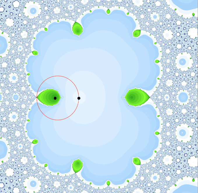
Figure 10. Detail of Julia set for the non-carpet example in Equation (7.4). The post-critical points $c$ and $0$ are marked in black, and the curve $\alpha$ is shown in red.

With a bit of work, one can show that $\overline{N}{}(f)=\sqrt{2}>1$.

7.2. Barycentric subdivision Julia set

We give details for the estimates for the conformal dimension of the Julia set of the map $f(z)=\frac{4}{27}\frac{(z^{2}-z+1)^{3}}{(z(z-1))^{2}}$ from the introduction.

The dynamics on the set of critical points is shown in the following diagram; here $\omega=\exp(2\pi i/6)$:

$$\vbox{\hbox{$\includegraphics{barycenter-1}$}}\quad\rightrightarrows\quad\vbox{\hbox{$\includegraphics{barycenter-0}$}}$$

Figure 11. Spines for the barycentric subdivision rational map

The map $f$ may be described as follows. Consider the degenerate spherical “triangle” $T_{0}$ (the upper half-plane) with vertices $(\infty,0,1)$ and angles $(\pi,\pi,\pi)$. If we give $\widehat{\mathbb{C}}$ the spherical metric to make this degenerate triangle equilateral, then the spherical triangle $T_{1}$ with vertices $(\infty,\omega,2)$ has corresponding angles $(\pi/6,\pi/4,\pi/2)$. There is a unique conformal map sending $T_{1}$ to $T_{0}$ and mapping the vertices $(\infty,\omega,2)\mapsto(\infty,0,1)$. Twelve reflected images of $T_{1}$ tile the sphere, and the map $f$ is the unique extension given by Schwarz reflection. The extended real axis is forward-invariant, and its preimage under $f$ divides the sphere into twelve small triangles, 6 in each of the upper- and lower-half planes. This induces a finite subdivision rule on the sphere, in the sense of [CFP01]. We equip the codomain with a cell structure with $0$-cells at $0,1,\infty$ and $1$-cells the corresponding segments of the extended real axis. Taking inverse images then refines each $2$-cell in a pattern that, combinatorially, effects barycentric subdivision; see Figure 2. The function $f$ is a Galois branched covering map; with deck group isomorphic to $S_{3}$ and acting by spherical isometries. It gives the $j$-invariant of an elliptic curve as a function of its $\lambda$-invariant; equivalently, it gives the shape invariant of a set of 4 points on $\widehat{\mathbb{C}}$ as a function of the cross-ratio of a corresponding list.

This map was studied by Cannon-Floyd-Parry [CFP01, Example 1.3.1], where they showed that the sequence of tilings $\mathcal{T}_{n}$ generated by iterated preimages is not conformal in Cannon’s sense: there is no metric on the sphere quasi-conformally equivalent to the standard metric in which combinatorial moduli of path families are comparable to analytic moduli. This is related to the fact that there are fixed critical points, which means the valence of $\mathcal{T}_{n}$ blows up as $n\to\infty$. Cannon-Floyd-Kenyon-Parry investigated it further [CFKP03, Figure 25], and proved that its Julia set is a Sierpiński carpet. Haïssinsky and the second author studied it as well [HP09, §4.6].

To give an upper bound for the conformal dimension for the Julia set of this map, we estimate $\overline{E}{}^{2}(f)$, which we know is less than one [Thu20, Theorem 1]. To get a concrete estimate, we look at a finite stage and compute $E^{2}_{2}[\phi^{n}]$ for some $n$. It turns out that $n=1$ is not enough to get an estimate less than $1$, so we consider $\phi^{2}\nobreak\mskip 2.0mu\mathpunct{}\nonscript\mkern-3.0mu{:}\allowbreak\mskip 6.0mu plus 1.0muG_{2}\to G_{0}$, as shown in Figure 12.

$$\vbox{\hbox{$\includegraphics{barycenter-3}$}}\quad\overset{\phi^{2}}{\rightarrow}\quad\vbox{\hbox{$\includegraphics{barycenter-0}$}}$$

Figure 12. The map $\phi^{2}\nobreak\mskip 2.0mu\mathpunct{}\nonscript\mkern-3.0mu{:}\allowbreak\mskip 6.0mu plus 1.0muG_{2}\to G_{0}$ for the barycentric subdivision map

We can take any elastic structure we like on $G_{0}$ and the pullback structure on $G_{2}$. It is most convenient to have $\alpha(e)=1$ for all three edges of $G_{0}$. In this case, by symmetry, an optimal map will map the larger dashed circle on the left of Figure 12 to the central edge on the right. (This circle passes through the midpoint of eight edges; the other halves of these edges of $G_{2}$ map to different edges of $G_{0}$.)

Finding the map that minimizes $E^{2}_{2}$ from a graph to an interval (with specified boundary behavior) is equivalent to finding the resistance of a resistor network (or alternatively a harmonic function on the graph), and can be solved with standard linear algebra techniques. This is easily computed to be $E^{2}_{2}[\phi^{2}]=10/13$, as shown in Figure 13. (The computation can be further simplified by using the symmetries evident in the figure.) Since the energy of any iterate gives an upper bound for the asymptotic energy [Thu20, Proposition 5.6], we therefore have $\overline{E}{}^{2}(f)\leq\sqrt{10/13}$.

Figure 13. The central portion of the concrete map realizing $E^{2}_{2}[\phi^{2}]$ for the barycentric subdivision map. The edges running off the top and bottom are half-edges in the domain of the map. The numbers are the relative lengths of the images of each edge (or half-edge); to get the actual length, divide by $26$. The map itself is projection onto the vertical axis.

Proposition 7.5.

For the barycentric carpet map $f$, we have

$$\operatorname{ARCdim}(J_{f})\leq p^{*}\leq\frac{2}{1-\log_{6}(10/13)}<1.745.$$

Proof.

By definition, we have $\overline{E}{}^{p^{*}}(f)=1$. Apply Proposition 7.1 with $q=2$ to find

$$\sqrt{10/13}\geq\overline{E}{}^{2}(f)\geq 6^{1/2-1/p^{*}}$$

which simplifies to the desired inequality after taking logs of both sides. ∎

Iterating further to estimate $\overline{E}{}^{2}(f)$ will improve the bound in Proposition 7.5, although it probably will not reach the optimal result, since Proposition 7.1 is not, in general, sharp.

To get a lower bound on conformal dimension, we compute $\overline{N}{}(f)$.

Proposition 7.6.

For the barycentric subdivision rational map, $\overline{N}{}(f)=2$.

Proof.

By examining Figure 11, it is easy to find a map in $[\phi]$ for which the inverse image of every generic point is two points. Thus $\overline{N}{}(f)\leq N[\phi]\leq 2$.

To get the opposite inequality, we will find $2^{n}$ edge-disjoint curves $\gamma_{i}^{n}$ on $G_{n}$ so that the curves $\phi^{n}(\gamma_{i}^{n})$ are all homotopic to a simple loop $\gamma_{0}$ on $G_{0}$; cf. the proof of Theorem C. This will immediately imply that $N[\phi^{n}]\geq 2^{n}$, as desired.

We find the $\gamma_{i}^{n}$ by inductively finding $2^{n}$ edge-disjoint paths connecting any two edges of the dual of the $n^{\mathrm{th}}$ barycentric subdivision of a triangle. This is trivial for $n=0$, and $n=1$ is shown in Figure 14. This also serves as the inductive step: at level $n$, in each triangle replace the concrete paths in Figure 14 with the family of $2^{n-1}$ parallel paths constructed by induction.

Figure 14. Connecting sides of a triangle in the barycentric subdivision with edge-disjoint paths. This is the case $n=1$ and the inductive step.

The closed curves $\gamma^{n}_{i}$ are obtained by doubling the triangle as usual. ∎

7.3. Fat real Devaney examples

We begin by recalling some specifics concerning the Devaney family $f_{\lambda}(z)=z^{2}+\lambda/z^{2}$. The points $0$ and $\infty$ are always critical points. The other critical points have orbits that start

(7.7) $$\lambda^{1/4}\mapsto\pm 2\sqrt{\lambda}\mapsto 4\lambda+1/4\eqqcolon x_{\lambda}\mapsto\ldots.$$

A sufficient condition for $J_{\lambda}\coloneqq J_{f_{\lambda}}$ to be hyperbolic and have a Sierpiński carpet Julia set is that $x_{\lambda}$ eventually iterates into the Fatou component containing the origin. Such parameter values form a countable collection of open disks called Sierpiński holes.

As shown by the first author and R. Devaney [DP09], given any finite word $w=\varepsilon_{0}\varepsilon_{1}\ldots\varepsilon_{n}$ in the alphabet $\{L,R\}$, there exists a unique $\lambda=\lambda_{w}$, necessarily real and negative, with the following property. For each $i=0,1,\ldots,n$, the image $f_{\lambda}^{i}(x_{\lambda})$ lies to the left ($L$) or right ($R$) of the origin, according to the symbol in the $i^{\mathrm{th}}$ position of $w$, and $f_{\lambda}^{n+1}(x_{\lambda})=0$. Let $\lambda_{n}^{\mathrm{skinny}}$ and $\lambda_{n}^{\mathrm{fat}}$ denote the parameter values corresponding to the words $LR^{n}$ and $R^{n}$, respectively.

In this section we prove the second half of Theorem E, dealing with the fat Devaney family. A virtual endomorphism spine for this rational map is shown in Figure 15 for $n=3$. As usual, the covering map $\pi$ preserves the decorations on the edges, and the map $\phi$ is the deformation retract onto $G_{0}$ as a spine for $S^{2}-P$, where $P$ consists of the indicated points in the diagram plus an extra point at $\infty$.

The critical points at the fourth roots of $\lambda$ are shown schematically on the diagram of $G_{1}$ with crosses; they map to the upper and lower critical values on the diagram of $G_{0}$, which in turn maps to the sequence of points on the right of $G_{0}$, eventually ending at the central critical point at $0$, which maps to $\infty$.

$$\vbox{\hbox{$\includegraphics{fat-1}$}}\quad\rightrightarrows\quad\vbox{\hbox{$\includegraphics{fat-0}$}}$$

Figure 15. Spines for the fat Devaney family, $R^{n}$, shown here with $n=3$. The post-critical set $P$ is shown with bullets. The crosses on the left are the pre-periodic critical points.

To bound the conformal dimension from below, we again find $\overline{N}{}(f_{\lambda})$ and use bounds on how quickly $\overline{E}{}^{q}$ decreases as a function of $q$. To find $\overline{N}{}$, consider the $n$-component multi-curve $C$ shown on the right of Figure 16. The curve $f^{-1}(C)$ is shown on the left of Figure 16. (As indicated, it is easy to find $f^{-1}(C)$ by using the fact that $G_{1}$ is a cover of $G_{0}$.) Each component of $f^{-1}(C)$ covers one of the components of $C$ with degree two. One of the components of $f^{-1}(C)$ is peripheral (the outer one), and the others are all components of $C$. Note that we have the following.

• $C$ is completely invariant (in the sense of Selinger [Sel12]): $f^{-1}(C)=C$, up to homotopy in $S^{2}-P_{f}$ and dropping inessential or peripheral components.

• $C$ is Cantor-type (in the sense of Cui-Peng-Tan [CPT16]): for some iterate, each component of $C$ has at least two preimages homotopic to itself.

$$\vbox{\hbox{$\includegraphics{fat-11}$}}\quad\longrightarrow\quad\vbox{\hbox{$\includegraphics{fat-10}$}}$$

Figure 16. Curves in $S^{2}-P$ for the fat Devaney family, and their inverse images. Each inverse image covers the original by degree $2$.

Lemma 7.8.

For the Devaney family at parameter $\lambda_{n}^{\mathrm{fat}}$, let $r_{n}$ be the largest root of $\lambda^{n+1}-2\lambda^{n}+1$. Then $\overline{N}{}(f_{\lambda_{n}^{\textrm{fat}}})\geq r_{n}$.

Proof.

Let $\{\gamma_{j}\}$ enumerate the components of $C$. Consider the positive matrix $A$ whose entry $A_{ij}$ records how many components of $f^{-1}(\gamma_{j})$ are homotopic to $\gamma_{i}$ (without accounting for the degree of the cover). Concretely, we have

$$A=\begin{pmatrix}1&1&\cdots&1&1\\ 1&0&\cdots&0&0\\ 0&1&\cdots&0&0\\ \vdots&\vdots&\ddots&\vdots&\vdots\\ 0&0&\cdots&1&0\end{pmatrix}.$$

Let $w$ be Perron-Frobenius eigenvector of $A$, with eigenvalue $\lambda$; concretely, $w_{i}=\lambda^{n-i-1}$ and $\lambda=r_{n}$ is the positive solution of

$$\lambda^{n}=\lambda^{n-1}+\lambda^{n-2}+\dots+\lambda+1.$$

Multiplying by $\lambda-1$ shows that this is the root given in the lemma statement. Then the weighted multi-curve $W=\sum w_{i}[\gamma_{i}]$ satisfies $f^{-1}(W)=\lambda W$. To be more precise, let $W_{1}$ be the pullback weighted curve on $G_{1}$; then $f^{-1}(W)=\phi(W_{1})=\lambda W$.

To see that $\lambda$ is a lower bound for $\overline{E}{}^{1}(f)$, we specialize the discussion in [Thu20, §7.5] to the present setting. Consider the natural embeddings $W\to G_{0}$ and the pullback embedding $W_{n}\to G_{n}$. We have

$$E^{1}_{1}[\phi^{n}]\geq\frac{E^{1}_{1}[\phi^{n}(W_{n})\to G_{0}]}{E^{1}_{1}[W_{n}\to G_{n}]}=\frac{E^{1}_{1}[\lambda^{n}W_{0}\to G_{0}]}{E^{1}_{1}[W_{n}\to G_{n}]}=\lambda^{n}.$$

Using the interpretation of $E^{1}_{1}$ via stretch factors—that is, a supremum of ratios of extremal lengths—as in §4.2 yields the result. ∎

Remark 7.9.

It is straightforward to find weights on the edges of $G_{0}$ to show that the inequality in Lemma 7.8 is an equality, but the lower bound is all we need for our result.

Lemma 7.10.

There exists a unique root $r_{n}$ of $g_{n}(\lambda)=\lambda^{n+1}-2\lambda^{n}+1$ in the interval $(1,2)$ and, for $n\geq 1$,

$$r_{n}\geq 2-2^{-n+1}.$$

Proof.

We have $g_{n}(2)=1>0$. For $n=1,2,3,4$, we can directly check that $g_{n}(2-2^{-n+1})\leq 0$. For $n\geq 5$,

$$g_{n}(2-2^{-n+1}) =2^{n+1}\biggl{(}1-\frac{1}{2^{n}}\biggr{)}^{n+1}\!-2^{n+1}\biggl{(}1-\frac{1}{2^{n}}\biggr{)}^{n}+1$$

$$\leq 2^{n+1}\biggl{(}1-\frac{n+1}{2^{n}}+\frac{n(n+1)}{2^{2n+1}}\biggr{)}-2^{n+1}\biggl{(}1-\frac{n}{2^{n}}\biggr{)}+1$$

$$=-1+\frac{n(n+1)}{2^{n}}<0.$$

It follows that there is a root of $g_{n}$ in $[2-2^{-n+1},2)$. Descartes’ rule of signs shows there is a unique root in $(1,2)$. ∎

Proof of Theorem E, fat family.

By Theorem B, Lemma 7.8, Lemma 7.10, and elementary estimates,

$$\operatorname{ARCdim}(f_{\lambda_{n}^{\textrm{fat}}})\geq\frac{1}{1-\log_{4}(\overline{N}{}(f_{\lambda_{n}^{\textrm{fat}}}))}\geq\frac{2}{2-\log_{2}r_{n}}\geq\frac{1}{1+2^{-n}}.\qed$$

We sketch two alternate proofs of the same lower bound on $\operatorname{ARCdim}(J(\lambda_{n}^{\mathrm{fat}}))$, using the same multi-curve. Fix $n$; we write $f=f_{\lambda_{n}^{\mathrm{fat}}}$, and set $J=J(f)$. We equip $J$ with a visual metric, as in §3.2; it belongs to the quasi-symmetric gauge of $f$, by Proposition 3.3.

Our first method is a variant of that employed in [HP08]. It associates to $C$ a critical exponent for the combinatorial modulus of the family of curves homotopic to $C$. This exponent is then a lower bound for $\operatorname{ARCdim}$. Abusing notation, let $[C]$ denote the family of curves in $J$ which are homotopic in $\widehat{\mathbb{C}}-P_{f}$ to some component $\gamma_{j}$ of the indicated multi-curve $C=\{\gamma_{j}\}$. Since each curve in the family is essential and non-peripheral, the diameters of elements of this family are bounded below, say by $\delta>0$, and so $[C]\subset\Gamma_{\delta}$. Let $\mathcal{U}_{m}$, $m\in\mathbb{N}$, denote the sequence of coverings as in §6; it is a collection of snapshots, by Proposition 6.3. For $Q>1$ let $A_{Q}$ denote the matrix whose $(i,j)$ entry is the sum of terms of the form $d_{ijk}^{1-Q}$ where $d_{ijk}=\deg(\delta_{k}\to\gamma_{j})$ and the curves $\delta_{k}$ range over preimages of $\gamma_{j}$ homotopic to $\gamma_{i}$ in the complement of the post-critical set. In our case these covering degrees are all equal to $2$, so $A_{Q}=2^{1-Q}A$. Thus the Perron-Frobenius eigenvalue $\lambda_{Q}$ of $A_{Q}$ is $2^{1-Q}r_{n}$ where $r_{n}$ is the root from Lemma 7.10; note this is strictly decreasing in $Q$. Setting this equal to $1$ and solving for $Q$ yields $Q_{*}=1+\log_{2}r_{n}$ for the critical exponent. Fix now $1<Q<Q_{*}$. Then as $m\to\infty$

$$\operatorname{mod}_{Q}(\Gamma_{\delta},\mathcal{U}_{m})\geq\operatorname{mod}_{Q}([C],\mathcal{U}_{m})\gtrsim 1,$$

where the last inequality is the statement of [HP08, Proposition 5.1]. By Corollary 5.12, we have $\operatorname{ARCdim}(J)>Q$ and hence $\operatorname{ARCdim}(J)\geq Q_{*}$.

Our second alternate proof we present here as a sketch; the motivation comes from [HP12]. Associated to the multi-curve $C$ is a holomorphic virtual endomorphism of spaces $\pi_{Y},\phi_{Y}\nobreak\mskip 2.0mu\mathpunct{}\nonscript\mkern-3.0mu{:}\allowbreak\mskip 6.0mu plus 1.0muY_{1}\rightrightarrows Y_{0}$ where $Y_{0}$ is a collection of Euclidean annuli of circumference $1$ (and geodesic boundary) indexed by the components of $C$ and $Y_{1}$ is a collection $R_{j}$ of pairwise disjoint right Euclidean sub-annuli of $Y_{0}$ indexed by the components of $f^{-1}(C)$ homotopic to $C$. We require that $\phi_{Y}$ induces a conformal inclusion $\overline{Y_{1}}\hookrightarrow Y_{0}$ and $\pi_{Y}\nobreak\mskip 2.0mu\mathpunct{}\nonscript\mkern-3.0mu{:}\allowbreak\mskip 6.0mu plus 1.0muY_{1}\to Y_{0}$ is conformal, a local expanding homothety in the Euclidean coordinates with constant factor $2$, and with each component mapping by degree $2$.

Associated to this conformal expanding dynamical system is a non-escaping set $X\subset Y_{0}$ and a self-map $g\nobreak\mskip 2.0mu\mathpunct{}\nonscript\mkern-3.0mu{:}\allowbreak\mskip 6.0mu plus 1.0muX\to X$. The set $X$ is isometric to a product $S^{1}\times\mathcal{C}$, where $S^{1}$ is the Euclidean circle of circumference $1$, and $\mathcal{C}$ is a Cantor set associated to a graph-directed iterated function system on a disjoint union of $\#C$ copies of $S^{1}$, with contraction maps having factor $2$, and where the copies map according to the combinatorics of the map $f^{-1}(C)\to C$. The Hausdorff dimension of $\mathcal{C}$ is equal to $\log_{2}r_{n}$, by a variant of the well-known “pressure formula”. It follows that the conformal dimension of $X$ is then equal to $1+\log_{2}r_{n}=Q_{*}$. There is a natural, non-surjective semiconjugacy $X\to J$ from $g$ to $f$.

If we knew this semiconjugacy was a homeomorphism, monotonicity of conformal dimension would imply the desired lower bound on $\operatorname{ARCdim}(J)$. Cui, Peng, and Tan [CPT16] show that there is a “thick” subset of $X$—the components living over “buried” points in the Cantor set $\mathcal{C}$—on which the semiconjugacy is injective; this should imply the desired lower bound. For example, passing to some high iterate, and deleting the extreme inner and outermost branches of the interval contraction mappings defining the corresponding Cantor set, one obtains a sub-system whose repellor maps injectively to $J$ and whose dimension is close to that of the original system $X$.

Remark 7.11.

It is challenging, using our techniques, to give a concrete upper bound estimate on $\operatorname{ARCdim}$ that is less than $2$. Although we know that $\overline{E}{}^{2}(f)<2$, at some iterate the actual energy must be less than 2, and at that iterate we could apply Proposition 7.1 to get an upper bound on $\operatorname{ARCdim}$. But it appears that we have to iterate quite a lot to get to these values and get a good upper bound on $\operatorname{ARCdim}$. In some sense, since the Julia set in these examples is a Sierpiński carpet of Hausdorff dimension close to $2$, it is not well-approximated by graphs.

7.4. Skinny Devaney examples

We now turn to the other half of Theorem E, dealing with the skinny Devaney family. Suitable spines in this case are shown in Figure 17 for $n=3$ (kneading sequence $LR^{3}$); again, the generalization is evident.

We will find an explicit $q\in(1,2)$, metric $\alpha$ on $G_{0}$, and map $\phi\nobreak\mskip 2.0mu\mathpunct{}\nonscript\mkern-3.0mu{:}\allowbreak\mskip 6.0mu plus 1.0muG_{1}\to G_{0}$ so that $E^{q}_{q}(\phi)=1$. The metric $\alpha$ is shown on the right of Figure 17, except that we have not yet determined the value $x$. The map $\phi$ is indicated schematically on the left of Figure 17: each region surrounded by a green loop is contracted to a point, and $\phi$ is optimized in the remaining regions.

$$\vbox{\hbox{$\includegraphics{skinny-2}$}}\quad\rightrightarrows\quad\vbox{\hbox{$\includegraphics{skinny-10}$}}$$

Figure 17. Spines for the skinny Devaney family, $LR^{n}$, shown here with $n=3$.

Inspection reveals that for most points $y\in G_{0}$, there is a unique point $x\in G_{1}$ with $\phi(x)=y$ and $\lvert\phi^{\prime}(x)\rvert=1$, compatible with $E^{q}_{q}(\phi)=1$. The exceptions are:

1. On the long left edge, there is a chain in $G_{1}$ of $n$ “double edges” (two edges connecting the same vertices), with each edge of length 1:

   

   This chain maps to an edge in $G_{0}$ of length $x$. (Note the right vertical edge gets mapped to a point.)

2. On each the four edges of the central square, there a chain in $G_{1}$ of an edge of length $x$, two parallel edges of length $2$, another edge of length $x$, and two parallel edges of length $1$:

   

   These chains each map to an edge in $G_{0}$ of length $1$.

We now solve for $x$ and $q$ to make the supremand in the definition of $E^{q}_{q}(\phi)$ equal to $1$ on these edges as well. We use the principle that two parallel edges of length $a$ and $b$ in a $q$-conformal graph can be replaced by a single edge of length

$$a\oplus_{q}b\coloneqq\bigl{(}a^{1-q}+b^{1-q}\bigr{)}^{1/(1-q)}$$

without changing the optimal $E^{q}_{q}$ energy of any map. (See [Thu20, Proposition 7.7]. The case $q=2$ is the standard parallel law for resistors.)

Thus, the $n$ double edges in (1) have an effective $q$-length of

$$x\coloneqq n\cdot(1\oplus_{q}1)=n\cdot 2^{1/(1-q)}.$$

We set $x$ to this value to make $E^{q}_{q}(\phi)=1$.

The chain of edges in (2) have an effective $q$-length of

$$x+(2\oplus_{q}2)+x+(1\oplus_{q}1)=2x+3\cdot 2^{1/(1-q)}=(2n+3)\cdot 2^{1/(1-q)}.$$

For $q=1+1/\log_{2}(2n+3)$, this quantity is equal to $1$, which makes $E^{q}_{q}(\phi)=1$, with the supremum in the definition of $E^{q}_{q}$ achieved everywhere on $G_{0}$.

Proposition 7.12.

For the skinny Devaney example $\lambda_{n}^{\mathrm{skinny}}$, for any $q>1+1/\log_{2}(2n+3)$, we can find a metric on $G_{0}$ in Figure 17 so that $E^{q}_{q}(\phi)<1$. Thus $\overline{E}{}^{q}[\pi,\phi]<1$ and

$$\operatorname{ARCdim}(J_{\lambda_{n}^{\mathrm{skinny}}})\leq 1+\frac{1}{\log_{2}(2n+3)}.$$

Proof.

For $q$ bigger than $1+1/\log_{2}(2n+3)$, it is straightforward to modify the metric on $G_{0}$ in Figure 17 by adjusting the lengths slightly to make $E^{q}_{q}[\phi]<1$. (For instance, on the chain of loops on the right side, multiply the length around the $k^{\mathrm{th}}$ dot in from the end by $(1+\varepsilon)^{k}$ for small $\varepsilon$.) Then for these $q$, we have $\overline{E}{}^{q}[\pi,\phi]\leq E^{q}_{q}[\phi]<1$ and $\operatorname{ARCdim}<q$, as desired. ∎

Remark 7.13.

One can also give a lower bound on $\operatorname{ARCdim}(J_{\lambda_{n}^{\mathrm{skinny}}})$ by estimating $\overline{N}{}[\pi,\phi]$.

7.5. Uniformly well-spread cut points

Definition 7.14.

A metric space $X$ is linearly connected if there exists a constant $L\geq 1$ such that for each pair of points $x,y\in X$, there is a continuum $J$ containing $\{x,y\}$ such that $\operatorname{diam}J\leq Ld(x,y)$.

If $X$ is connected and $f\nobreak\mskip 2.0mu\mathpunct{}\nonscript\mkern-3.0mu{:}\allowbreak\mskip 6.0mu plus 1.0muX\to X$ is metrically cxc, then $X$ is linearly connected [HP09].

Definition 7.15.

A compact, connected metric space $X$ is said to satisfy the uniformly well-spread cut points condition (UWSCP) if there exists a constant $C\geq 1$ such that for each $x\in X$ and each $r>0$, there exists a set $A\subset X$ with $\#A\leq C$ such that no component of $X-A$ meets both $B(x,r/2)$ and $X-\overline{B}(x,r)$.

The following result is [Car14, Theorem 1.2].

Theorem 7.16.

If $X$ is doubling, compact, connected, linearly connected, and satisfies the UWSCP condition, then $\operatorname{ARCdim}(X)=1$.

7.6. Matings

In this section, we give an example showing that among Julia sets of hyperbolic rational functions, the UWSCP is sufficient but not necessary for $\operatorname{ARCdim}(J)=1$. To our knowledge, this is the first result of its kind. We start by recalling generalities on matings.

Formal mating

The operation of formal mating takes as input two monic critically finite polynomials $f_{1},f_{2}$ of the same degree $d\geq 2$ acting on the complex plane, and returns as output a topological Thurston map $f_{1}\amalg f_{2}\nobreak\mskip 2.0mu\mathpunct{}\nonscript\mkern-3.0mu{:}\allowbreak\mskip 6.0mu plus 1.0muS^{2}\to S^{2}$ on the sphere obtained by gluing together the actions of $f_{1}$ and $f_{2}$ on the plane compactified by the circle at infinity $\mathbb{S}^{1}_{\infty}$, where the gluing is via $\infty\cdot e^{2\pi i\theta}\sim\infty\cdot e^{-2\pi i\theta}$. Identifying $\mathbb{S}^{1}_{\infty}=\mathbb{R}/\mathbb{Z}$, the restriction of the formal mating to the circle at infinity is given by $\theta\mapsto\tau_{d}(\theta)\coloneqq d\theta$ modulo $1$. We refer the reader to [BEK⁺12] for a survey containing facts mentioned below. Our focus here is exclusively on the case when the $f_{i}$ are hyperbolic; this assumption simplifies the discussion. Abusing terminology, given a hyperbolic critically finite polynomial $f$, we call a bounded Fatou component a basin of $f$.

Ray equivalence relation and geometric mating

The sphere $S^{2}$ on which $f\amalg g$ acts comes equipped with a natural invariant “ray-equivalence” relation, $\sim_{\mathrm{ray}}$. If $R\nobreak\mskip 2.0mu\mathpunct{}\nonscript\mkern-3.0mu{:}\allowbreak\mskip 6.0mu plus 1.0mu\widehat{\mathbb{C}}\to\widehat{\mathbb{C}}$ is a rational map such that quotienting by the ray equivalence relation yields a continuous semiconjugacy $\rho\nobreak\mskip 2.0mu\mathpunct{}\nonscript\mkern-3.0mu{:}\allowbreak\mskip 6.0mu plus 1.0muS^{2}\to\widehat{\mathbb{C}}$ from $f\amalg g$ to $R$ that is conformal on the basins of the $f_{i}$, we say $f_{1},f_{2}$ are geometrically mateable and that $R$ is the geometric mating of $f_{1}$ and $f_{2}$. See Figure 3. The restriction $\rho\nobreak\mskip 2.0mu\mathpunct{}\nonscript\mkern-3.0mu{:}\allowbreak\mskip 6.0mu plus 1.0mu\mathbb{S}^{1}_{\infty}\to J(R)$ is surjective; its fibers are the intersections of the ray-equivalence classes with $\mathbb{S}^{1}_{\infty}$. It is interesting to ask how big the fibers can be.

The following is a special case of a general principle, to our knowledge first articulated by D. Fried [Fri87]: that expanding dynamical systems on reasonable spaces are “finitely presented”, in the following precise sense: they are quotients of an expanding subshift of finite type, and there is another subshift which encodes when two points lie in the same fiber. Restricted to the case of matings, we were surprised not to find this result in the literature; c.f. the survey [PM12, Remark 4.13] where the possibility of ray equivalence classes of unbounded size is entertained. Explicit bounds for the closely related question of the length of ray connections are established in certain cases by W. Jung [Jun17].

Proposition 7.17.

Suppose $f_{1},f_{2}$ are monic hyperbolic critically finite polynomials of degree $d\geq 2$ that are geometrically mateable, with geometric mating $R$. Then there exists a constant $C=C(f_{1},f_{2})$ such that fibers of $\rho\nobreak\mskip 2.0mu\mathpunct{}\nonscript\mkern-3.0mu{:}\allowbreak\mskip 6.0mu plus 1.0mu\mathbb{S}^{1}_{\infty}\to J(R)$ have cardinality at most $C$.

For the proof, we apply a general result of Nekrashevych. To motivate the technique, and because we need it anyway, we begin by presenting a construction of a semiconjugacy $\pi\nobreak\mskip 2.0mu\mathpunct{}\nonscript\mkern-3.0mu{:}\allowbreak\mskip 6.0mu plus 1.0mu\Sigma_{d}\to\mathbb{S}^{1}_{\infty}$ from the full 1-sided shift on $d$ symbols to the map $\tau_{d}$. We then analyze the composition

$$\Sigma_{d}\stackrel{{\scriptstyle\pi}}{{\longrightarrow}}\mathbb{S}^{1}_{\infty}\stackrel{{\scriptstyle\rho}}{{\longrightarrow}}J(R).$$

Proof.

We take $x_{0}\coloneqq\infty e^{2\pi i0}$ as a basepoint, and denote by $x_{k}$ for $k=0,\ldots,d-1$ its $d$ preimages under the map $\tau_{d}$. There is a canonical positively oriented (counterclockwise) arc $\alpha_{k}\subset\mathbb{S}^{1}_{\infty}$ joining the basepoint $x_{0}$ to each $x_{k}$. Fix an iterate $n\geq 1$. Lifting the $\alpha_{k}$ under $\tau,\tau^{\circ 2},\ldots,\tau^{\circ n}$ and concatenating the lifts gives an identification of $\tau^{-n}(x_{0})$ with $\{0,1,\ldots,d-1\}^{n}$ given by taking endpoints of iteratively concatenated lifts. The lengths of the concatenations are uniformly bounded, since the $n$th stage has length bounded by a convergent geometric series with ratio $1/d$, and passing to the limit we obtain the desired semiconjugacy $\pi:\Sigma_{d}\to\mathbb{S}^{1}_{\infty}$ from the shift to $\tau_{d}$. (More simply, we can also see this semiconjugacy a writing an element in $\mathbb{R}/\mathbb{Z}$ in base $d$.)

Our strategy is to now “push” this construction down to the dynamical plane of $R$ via the semiconjugacy $\rho$. Denote by $P$ the post-critical set of $R$. For each $k=0,1,\ldots,d-1$ let $\beta_{k}$ be a smooth path in $\widehat{\mathbb{C}}-P$ homotopic relative to endpoints to the arc $\rho(\alpha_{k})$. Note that since $R$ is hyperbolic, it is expanding outside of a neighborhood of $P$. Applying the same iteratively-lifting-and-concatenating construction from the previous paragraph using the $\beta_{k}$ and $R$ in place of the $\alpha_{k}$ and $\tau_{d}$, we get a well-defined composition $\rho\circ\pi\nobreak\mskip 2.0mu\mathpunct{}\nonscript\mkern-3.0mu{:}\allowbreak\mskip 6.0mu plus 1.0mu\Sigma_{d}\to J(R)$ induced by taking endpoints of infinitely iterated concatenated lifts of the $\beta_{k}$.

Nekrashevych [Nek05, Proposition 3.6.2] shows that in this setting, there is a finite automaton, called the nucleus, whose one-sided infinite paths encode the equivalence relation on $\Sigma_{d}$ identifying points in the fiber of the composition $\rho\circ\pi$. It follows that the size of these equivalence classes are uniformly bounded by the size of the nucleus. The fibers of $\rho$ are no larger than those of $\rho\circ\pi$, yielding the result. ∎

See also [Nek05, §6.13], in which details for a specific example of mating are presented.

Quadratic matings

The following theorem is due to Tan Lei [Tan92] and M. Shishikura [Shi00], and was proven using ideas of M. Rees.

Theorem 7.18.

Two critically finite quadratic polynomials $f_{1},f_{2}$ are mateable if and only if they do not lie in conjugate limbs of the Mandelbrot set.

To a hyperbolic critically finite quadratic polynomial $f$ is associated a unique nontrivial interval $[a,b]\subset\mathbb{R}/\mathbb{Z}$: the external rays of angles $a$ and $b$ land at a common periodic point on the boundary of the immediate basin $U$ containing the critical value of $f$, and separate $U$ from all other periodic attracting basins. For the basilica, $[a,b]=[1/3,2/3]$, while for the airplane, $[a,b]=[3/7,4/7]$. The denominators of $a$ and $b$ take the form $2^{n}-1$ where $n$ is the period of the finite critical point.

Generalized rabbits

If the hyperbolic component containing $f$ has closure meeting the main cardioid component containing $z^{2}$, we call $f$ a generalized rabbit. In this case, one may encode $f$ by rational numbers in a different way.

For each $p/q\in\mathbb{Q}/\mathbb{Z}-\{0\}$, there is a unique hyperbolic critically finite quadratic polynomial $f=f_{p/q}$ such that there are $q$ periodic basins meeting at a common repelling fixed-point $\alpha$, and such that the dynamics on the set of these $q$ periodic basins, when equipped with the natural local cyclic ordering near $\alpha$, is given by a rotation with angle $p/q$. This fact can be deduced from the classification of critically finite hyperbolic quadratic polynomials via their so-called invariant laminations; see [Thu09]. The basilica polynomial is $f_{1/2}$, while the rabbit polynomial is $f_{1/3}$.

A special feature of generalized rabbit polynomials is the following. If $f$ is a generalized rabbit polynomial and $\theta_{1}\sim\theta_{2}$ is any nontrivial ray-equivalent pair of angles, so that the corresponding rays land on a common point $z$ in the Julia set of $f$, then the point $z$ is on the boundary of a basin of $f$. This fact need not hold for other pcf polynomials like the airplane.

Proposition 7.19.

For $i=1,2$ suppose $p_{i}/q_{i}\in\mathbb{Q}/\mathbb{Z}-\{0\}$ and suppose $q_{1},q_{2}$ are coprime. Let $f_{i}$ be the corresponding generalized rabbit quadratic polynomials, and $R$ the geometric mating of $f_{1}$ and $f_{2}$. Then the basins of $f_{1}$ and $f_{2}$ do not touch in the Julia set of $R$.

Note that the mating exists by Theorem 7.18. In the proof below applied to the mating of the basilica and rabbit, the key observation is that the intervals $[1/3,2/3]$ and $[1-2/7,1-1/7]$ are disjoint.

Proof.

We argue by contradiction. Let $U_{i}$ be the immediate basin containing the finite critical value of $f_{i}$. Suppose $z\in J(R)$ is a point that is simultaneously on the boundary of a basin for $f_{1}$ and a basin for $f_{2}$. Since, by Proposition 7.17, the ray equivalence classes are finite and the $f_{i}$ are generalized rabbits, this implies there exists an angle $\theta$ such that the ray of angle $\theta$ for $f_{1}$ lands on a point $z_{1}$ on the boundary of a basin of $f_{1}$, and the ray of angle $-\theta$ for $f_{2}$ lands on a point $z_{2}$ on the boundary of a basin of $f_{2}$. By iterating this ray-pair forward under the formal mating, we may assume that $z\in\partial U_{1}$. Since $q_{1}$ and $q_{2}$ are co-prime, by passing to a further iterate, we may assume that $z\in\partial U_{1}\cap\partial U_{2}$.

In the dynamical plane of $f_{i}$, let $(a_{i},b_{i})$ be the ray-pair of angles landing at the point $\alpha_{i}$ separating $U_{i}$ from the remaining immediate attracting basins of $f_{i}$, as recalled above. In giving coordinates for the circle at infinity $\mathbb{R}/\mathbb{Z}$, we parameterize to agree with the usual counterclockwise orientation on $f_{1}$ and disagree for $f_{2}$, so that the coordinates match when we mate. For example, if $f_{1}$ is the basilica and $f_{2}$ the rabbit, then $(a_{1},b_{1})=(1/3,2/3)$ and $(a_{2},b_{2})=(1-2/7,1-1/7)$. Then the set of angles of rays landing on $\partial U_{i}$ is a subset of $[a_{i},b_{i}]$. The condition that $q_{1}$ and $q_{2}$ are coprime implies that $f_{1}$ and $f_{2}$ are not in conjugate limbs of the Mandelbrot set, and hence that $[a_{1},b_{1}]$ and $[a_{2},b_{2}]$ are disjoint. But the previous paragraph shows $\theta$ belongs to both of these intervals. This is impossible. ∎

Proposition 1.2 is then an immediate consequence of the following two Propositions.

Proposition 7.20.

Suppose $f_{1}$, $f_{2}$, and $R$ are as in Proposition 7.19. Then the Julia set $J_{R}$ of $R$ does not satisfy UWSCP. In particular, the Julia set of the basilica mated with the rabbit does not satisfy UWSCP.

Proof.

Suppose $J_{R}$ satisfies UWSCP, and $C$, $x$, $r$, and $A$ be any data as in Definition 7.15. Then there exists a Jordan curve $\gamma$ surrounding $x$ meeting $J_{R}$ only in the finite set $A$. Since the basins of the $f_{1}$ and $f_{2}$ do not touch, the loop $\gamma$ lies in the closure of finitely many immediate basins of one of the $f_{i}$, say $f_{1}$.

Since $J_{R}$ is the common boundary of the union of the basins of $f_{1}$ and of $f_{2}$, each component of $\overline{\mathbb{C}}-\gamma$ contains a basin of $f_{2}$, say $U$ and $V$. On the one hand, $U$ and $V$ are joined by a path $\beta$ lying in the closure of finitely many basins of $f_{2}$ and meeting $J(R)$ in finitely many points, since this is true in the dynamical plane of $f_{2}$. On the other hand, any such path intersects $\gamma$ and thus passes through a point of $A$. It follows that the basins of $f_{1}$ and $f_{2}$ touch in this point of $A$. By Proposition 7.19, this is impossible. ∎

Proposition 7.21.

The virtual endomorphism $F_{RB}$ of the mating of the rabbit and the basilica satisfies $\overline{N}[F_{RB}]=1$ and, for $q>1$, $\overline{E}{}^{q}[F_{RB}]<1$, and so $\operatorname{ARCdim}(\mathcal{J}_{RB})=1$.

Figure 18. Spines for the mating of the rabbit and the basilica

Proof.

The spines for this mating are shown in Figure 18, with a black equator and colored rays. We may take the map $\phi$ in its homotopy class to be the map that “pushes” the extra colored edge towards the equator. If we do this suitably, each colored point in $G_{0}$ has one (colored) preimage, and each point on the equator has at most three preimages, one on the equator and two colored. It follows by iteration that $N(\phi^{n})=2n+1$ and so $\overline{N}[F_{RB}]=1$. For the statement about $\overline{E}{}^{q}$, we proceed as in [Thu16, Example 2.4]. Fix $q>1$, and consider a metric on $G_{0}$ where the colored edges have equal length $L$. For the map $\phi$ described above, $\operatorname{Fill}^{q}(\phi)=1$ on the colored edges, and, for $L$ sufficiently large, $\operatorname{Fill}^{q}(\phi)\approx 2^{1-q}<1$. We can homotop $\phi$ to make $\operatorname{Fill}^{q}$ less than one everywhere by pulling the images of the vertices on the equator very slightly in along the colored edges; this decreases the derivative on the colored edge, while increasing the derivative on the equator (but keeping it less than $1$). Then $\overline{E}{}^{q}[F_{RB}]\leq E[\phi]<1$, as desired. ∎

Remark 7.22.

The proof in Proposition 7.21 works for any pair of polynomials $f_{1},f_{2}$ in the hypothesis of Proposition 7.19: all such matings have $\overline{N}[\pi,\phi]=1$. However, if we mate two polynomials that are far out in the limbs, we may end up with a Sierpiński carpet. Figure 19 gives empirical evidence for this assertion. It shows the Julia set of the result of mating of the airplane polynomial $f_{1}$ and another polynomial $f_{2}$, with corresponding angles $(a_{1},b_{1})=(3/7,4/7)$ and $(a_{2},b_{2})=(3/31,4/31)$. The mating appears to be a Sierpiński carpet. (This example was found by Insung Park and Caroline Davis.)

Figure 19. The Julia set of airplane mate a kokopelli-like polynomial. Picture by Arnaud Chéritat.

Conjecture 7.23.

The Julia set of a hyperbolic rational map satisfies UWSCP iff its virtual endomorphism has uniformly bounded $N[\phi^{n}]$ (independent of $n$).

References

- [AH94] N. Aoki and K. Hiraide, Topological theory of dynamical systems, North-Holland Mathematical Library, vol. 52, North-Holland Publishing Co., Amsterdam, 1994.
- [BEK+12] Xavier Buff, Adam L. Epstein, Sarah Koch, Daniel Meyer, Kevin Pilgrim, Mary Rees, and Tan Lei, Questions about polynomial matings, Ann. Fac. Sci. Toulouse Math. (6) 21 (2012), no. 5, 1149–1176.
- [BK13] Marc Bourdon and Bruce Kleiner, Combinatorial modulus, the combinatorial Loewner property, and Coxeter groups, Groups Geom. Dyn. 7 (2013), no. 1, 39–107, doi:10.4171/GGD/177.
- [BK15] by same author, Some applications of -cohomology to boundaries of Gromov hyperbolic spaces, Groups Geom. Dyn. 9 (2015), no. 2, 435–478, doi:10.4171/GGD/318.
- [BLM16] Mario Bonk, Mikhail Lyubich, and Sergei Merenkov, Quasisymmetries of Sierpiński carpet Julia sets, Adv. Math. 301 (2016), 383–422, doi:10.1016/j.aim.2016.06.007.
- [BM17] Mario Bonk and Daniel Meyer, Expanding Thurston maps, Mathematical Surveys and Monographs, vol. 225, American Mathematical Society, Providence, RI, 2017, arXiv:1009.3647.
- [Car13] Matias Carrasco, On the conformal gauge of a compact metric space, Ann. Sci. Éc. Norm. Supér. (4) 46 (2013), no. 3, 495–548.
- [Car14] by same author, Conformal dimension and canonical splittings of hyperbolic groups, Geom. Funct. Anal. 24 (2014), no. 3, 922–945, arXiv:1301.6492, doi:10.1007/s00039-014-0282-7.
- [CFKP03] J. W. Cannon, W. J. Floyd, R. Kenyon, and W. R. Parry, Constructing rational maps from subdivision rules, Conform. Geom. Dyn. 7 (2003), 76–102, doi:10.1090/S1088-4173-03-00082-1.
- [CFP01] J. W. Cannon, W. J. Floyd, and W. R. Parry, Finite subdivision rules, Conform. Geom. Dyn. 5 (2001), 153–196, doi:10.1090/S1088-4173-01-00055-8.
- [CPT16] Guizhen Cui, Wenjuan Peng, and Tan Lei, Renormalization and wandering Jordan curves of rational maps, Comm. Math. Phys. 344 (2016), no. 1, 67–115, arXiv:1403.5024, doi:10.1007/s00220-016-2623-x.
- [CS98] J. W. Cannon and E. L. Swenson, Recognizing constant curvature discrete groups in dimension , Trans. Amer. Math. Soc. 350 (1998), no. 2, 809–849, doi:10.1090/S0002-9947-98-02107-2.
- [DH93] A. Douady and John Hubbard, A proof of Thurston’s topological characterization of rational functions, Acta. Math. 171 (1993), no. 2, 263–297.
- [DK18] Cornelia Druţu and Michael Kapovich, Geometric group theory, American Mathematical Society Colloquium Publications, vol. 63, American Mathematical Society, Providence, RI, 2018, with an appendix by Bogdan Nica.
- [DLU05] Robert L. Devaney, Daniel M. Look, and David Uminsky, The escape trichotomy for singularly perturbed rational maps, Indiana Univ. Math. J. 54 (2005), no. 6, 1621–1634, doi:10.1512/iumj.2005.54.2615.
- [DP09] Robert L. Devaney and Kevin M. Pilgrim, Dynamic classification of escape time Sierpiński curve Julia sets, Fund. Math. 202 (2009), no. 2, 181–198, doi:10.4064/fm202-2-5.
- [DPT+19] Tushar Das, Feliks Przytycki, Giulio Tiozzo, Mariusz Urbański, and Anna Zdunik, Thermodynamic formalism for coarse expanding dynamical systemes, Preprint, 2019, arXiv:1908.08270.
- [Fri87] David Fried, Finitely presented dynamical systems, Ergodic Theory Dynam. Systems 7 (1987), no. 4, 489–507, doi:10.1017/S014338570000417X.
- [GHMZ18] Yan Gao, Peter Haïssinsky, Daniel Meyer, and Jinsong Zeng, Invariant Jordan curves of Sierpiński carpet rational maps, Ergodic Theory Dynam. Systems 38 (2018), no. 2, 583–600, arXiv:1511.02457, doi:10.1017/etds.2016.47.
- [Hat02] Allen Hatcher, Algebraic topology, Cambridge University Press, Cambridge, 2002.
- [Hei01] Juha Heinonen, Lectures on analysis on metric spaces, Universitext, Springer-Verlag, New York, 2001.
- [HP08] Peter Haïssinsky and Kevin M. Pilgrim, Thurston obstructions and Ahlfors regular conformal dimension, J. Math. Pures Appl. (9) 90 (2008), no. 3, 229–241, doi:10.1016/j.matpur.2008.04.006.
- [HP09] Peter Haïssinsky and Kevin M. Pilgrim, Coarse expanding conformal dynamics, Astérisque 325 (2009), viii+139 pp.
- [HP11] by same author, Finite type coarse expanding conformal dynamics, Groups Geom. Dyn. 5 (2011), no. 3, 603–661, doi:10.4171/GGD/141.
- [HP12] by same author, Examples of coarse expanding conformal maps, Discrete Contin. Dyn. Syst. 32 (2012), no. 7, 2403–2416, doi:10.3934/dcds.2012.32.2403.
- [HS01] Stefan-M. Heinemann and Bernd O. Stratmann, Geometric exponents for hyperbolic Julia sets, Illinois J. Math. 45 (2001), no. 3, 775–785.
- [IS10] Yutaka Ishii and John Smillie, Homotopy shadowing, Amer. J. Math. 132 (2010), no. 4, 987–1029, doi:10.1353/ajm.0.0126.
- [Jun17] Wolf Jung, Quadratic matings and ray connections, Preprint, 2017, arXiv:1707.00630.
- [Kle06] Bruce Kleiner, The asymptotic geometry of negatively curved spaces: uniformization, geometrization and rigidity, International Congress of Mathematicians. Vol. II, Eur. Math. Soc., Zürich, 2006, pp. 743–768.
- [Kwa20] Jaroslaw Kwapisz, Conformal dimension via -resistance: Sierpiński carpet, Ann. Acad. Sci. Fenn. Math. 45 (2020), no. 1, 3–51, doi:10.5186/aasfm.2020.4515.
- [Mac10] John M. Mackay, Spaces and groups with conformal dimension greater than one, Duke Math. J. 153 (2010), no. 2, 211–227, doi:10.1215/00127094-2010-023.
- [Mil93] John Milnor, Geometry and dynamics of quadratic rational maps, Experiment. Math. 2 (1993), no. 1, 37–83, with an appendix by the author and Tan Lei.
- [MT10] John M. Mackay and Jeremy T. Tyson, Conformal dimension: Theory and application, University Lecture Series, vol. 54, American Mathematical Society, Providence, RI, 2010, doi:10.1090/ulect/054.
- [Nek05] Volodymyr Nekrashevych, Self-similar groups, Mathematical Surveys and Monographs, vol. 117, American Mathematical Society, Providence, RI, 2005, doi:10.1090/surv/117.
- [Nek14] by same author, Combinatorial models of expanding dynamical systems, Ergodic Theory Dynam. Systems 34 (2014), no. 3, 938–985, arXiv:0810.4936, doi:10.1017/etds.2012.163.
- [Noo] Matt Noonan, FractalStream, Program for exploring complex dynamical systems, http://pi.math.cornell.edu/~noonan/fstream.html.
- [Par21] Insung Park, Thurston and Levy obstructions of finite subdivision rules, Ph.D. thesis, Indiana University, 2021.
- [Pil94] Kevin Pilgrim, Cylinders for iterated rational maps, Ph.D. thesis, University of California, Berkeley, 1994.
- [PM12] Carsten Lunde Petersen and Daniel Meyer, On the notions of mating, Ann. Fac. Sci. Toulouse Math. (6) 21 (2012), no. 5, 839–876, arXiv:1307.7934, doi:10.5802/afst.1355.
- [PU10] Feliks Przytycki and Mariusz Urbański, Conformal fractals: ergodic theory methods, London Mathematical Society Lecture Note Series, vol. 371, Cambridge University Press, Cambridge, 2010, doi:10.1017/CBO9781139193184.
- [PUZ89] Feliks Przytycki, Mariusz Urbański, and Anna Zdunik, Harmonic, Gibbs and Hausdorff measures on repellers for holomorphic maps. I, Ann. of Math. (2) 130 (1989), no. 1, 1–40, doi:10.2307/1971475.
- [Sel12] Nikita Selinger, Thurston’s pullback map on the augmented Teichmüller space and applications, Invent. Math. 189 (2012), no. 1, 111–142, arXiv:1010.1690, doi:10.1007/s00222-011-0362-3.
- [Shi00] Mitsuhiro Shishikura, On a theorem of M. Rees for matings of polynomials, The Mandelbrot Set, Theme and Variations, London Math. Soc. Lecture Note Ser., vol. 274, Cambridge Univ. Press, Cambridge, 2000, pp. 289–305.
- [Tan92] Tan Lei, Matings of quadratic polynomials, Ergodic Theory Dynam. Systems 12 (1992), no. 3, 589–620.
- [Thu09] William P. Thurston, On the geometry and dynamics of iterated rational maps, Complex dynamics, A K Peters, Wellesley, MA, 2009, Edited by Dierk Schleicher and Nikita Selinger and with an appendix by Schleicher, pp. 3–137, doi:10.1201/b10617-3.
- [Thu16] Dylan P. Thurston, From rubber bands to rational maps: A research report, Res. Math. Sci. 3 (2016), Art. 15, arXiv:1502.02561, doi:10.1186/s40687-015-0039-4.
- [Thu19] by same author, Elastic graphs, Forum Math. Sigma 7 (2019), e24, 84, arXiv:1607.00340, doi:10.1017/fms.2019.4.
- [Thu20] by same author, A positive characterization of rational maps, Ann. of Math. (2) 192 (2020), no. 1, 1–46, arXiv:1612.04424, doi:10.4007/annals.2020.192.1.1.