Revisiting the algebraic structure of the generalized uncertainty principle

Abstract

We compare different formulations of the generalized uncertainty principle that have an underlying algebraic structure. We show that the formulation by Kempf, Mangano and Mann (KMM) [Phys. Rev. D 52 (1995)], quite popular for phenomenological studies, satisfies the Jacobi identities only for spin zero particles. In contrast, the formulation proposed earlier by one of us (MM) [Phys. Lett. B 319 (1993)] has an underlying algebraic structure valid for particles of all spins, and is in this sense more fundamental. The latter is also much more constrained, resulting into only two possible solutions, one expressing the existence of a minimum length, and the other expressing a form of quantum-to-classical transition. We also discuss how this more stringent algebraic formulation has an intriguing physical interpretation in terms of a discretized time at the Planck scale.

I Introduction

The idea of a generalized uncertainty principle (GUP), of the form

$$\Delta x\,\raise 1.72218pt\hbox{$>$}\kern-6.99997pt\lower 2.6694pt\hbox{$\sim$}\,\frac{\hbar}{2\Delta p}+{\rm const.}\times G_{N}\Delta p$$ (1)

(where $G_{N}$ is Newton’s constant), and its associated minimum resolvable length, emerges from the computation of scattering amplitudes in string theory at Planckian energies Veneziano:1986zf ; Amati:1987wq ; Amati:1988tn ; Gross:1987kza ; Gross:1987ar and from Gedanken experiment with black holes and Hawking radiation Maggiore:1993rv ; Adler:1999bu (although the idea of a minimum length in gravity has a very long history, see Hossenfelder:2012jw ; Hagar:2014 for historical discussions). In these frameworks, the term proportional to $G_{N}$ corresponds to a first-order quantum gravity correction, valid in the limit $\Delta p/(M_{\rm P}c)\ll 1$, where $M_{\rm P}=\sqrt{\hbar c/G_{N}}$ is the Planck mass. Therefore, Eq. (1) should be understood as

$$\Delta x\geq\frac{\hbar}{2\Delta p}\left[1+\beta_{0}\left(\frac{\Delta p}{M_{\rm P}c}\right)^{2}+{\cal O}\left(\frac{\Delta p}{M_{\rm P}c}\right)^{4}\right]\;,$$ (2)

where $\beta_{0}$ is a dimensionless constant [related to the constant appearing in Eq. (1) by ${\rm const.}=\beta_{0}/(2c^{3})$].

It is natural to ask whether there is an algebraic structure underlying the GUP, much as the canonical commutator $[x_{i},p_{j}]=i\hbar\delta_{ij}$ underlies the standard Heisenberg uncertainty relation, and, in the affirmative case, if, under some reasonable assumptions, the algebraic structure is sufficiently constraining to determine (almost) uniquely the structure of the higher-order terms in Eq. (1). This question was first posed, and answered affirmatively, by one of us (MM) in Maggiore:1993kv (see also Maggiore:1993zu ). A different answer to the same question was later provided by Kempf, Mangano and Mann (KMM) in Kempf:1994su .

In this paper we further elaborate on the algebraic formulations of the GUP. In section II we compare the MM and KMM formulations of the GUP, and argue that the former is more fundamental, as the resulting commutators satisfy the Jacobi identities in full generality, while, in the approach of KMM, it is implicitly assumed that the $x_{i}$ are the coordinates of a spin-zero particle. If the existence of a minimum length should emerge from a fundamental theory of quantum gravity as a basic property of space-time, it must hold independently of the type of particle used to probe it, and, in this sense, the formulation in Maggiore:1993kv seems more suitable to emerge from a fundamental theory. As we will see, this formulation is also more restrictive, fixing uniquely (modulo a sign) the $[x_{i},x_{j}]$ and the $[x_{i},p_{j}]$ commutators, while the KMM approach involves an arbitrary function of momentum. Out of the two solutions allowed by the Jacobi identities in the approach of Maggiore:1993kv , only one describes the existence of a minimum length. The other, which differs in a crucial sign, was already mentioned in Maggiore:1993kv , but received little attention. In section III we will discuss the latter solution in more detail, and we show that it can be seen as describing a transition from quantum to classical mechanics, with all commutators vanishing at a critical energy. In section IV, elaborating on results presented in Maggiore:2002qr , we will see how the two solutions allowed by the Jacobi identities can be understood as emerging in a setting in which time becomes discrete at the Planck scale. In secttion V we will examine the effect of GUPs to composite objects, confirming previous results obtained in the KMM framework Amelino-Camelia:2013fxa , that indicate a strong suppression of GUP effects at macroscopic scales when the deformed commutators are applied to the constituent particles. Some further generalization of the algebraic structure underlying the GUP are discussed in Section VI. Finally, section VII summarizes our conclusions.

II Comparison of different algebraic approaches to the GUP

Let us begin by recalling the MM approach followed in Ref. Maggiore:1993kv to find an algebraic structure underlying the GUP. One starts by assuming that: (1) the three-dimensional rotation group is not deformed, so the rotation generators ${\bf J}$ satisfy the undeformed commutation relations $[J_{i},J_{j}]=i\epsilon_{ijk}J_{k}$, and coordinates and momenta satisfy the undeformed commutation relations of spatial vectors, $\left[J_{i},x_{j}\right]=i\epsilon_{ijk}x_{k},\left[J_{i},p_{j}\right]=i\epsilon_{ijk}p_{k}$. (2) The momenta commutes among themselves: $\left[p_{i},p_{j}\right]=0$, so that also the translation group is not deformed. (3) The $\left[x,x\right]$ and $\left[x,p\right]$ commutators depend on a deformation parameter $\kappa$ with dimensions of mass. In the limit $\kappa\rightarrow\infty$ (that is, $\kappa c^{2}$ much larger than any energy in the problem), the canonical commutation relations are recovered. With these assumptions, one is led to look for an expression for the $[x,x]$ and $[x,p]$ commutators of the form

$$\left[x_{i},x_{j}\right] = \left(\frac{\hbar}{\kappa c}\right)^{2}\,a(p)\,i\epsilon_{ijk}J_{k}\;,$$ (3)

$$\left[x_{i},p_{j}\right] = i\hbar\,\delta_{ij}f(p)\;.$$ (4)

Having assumed rotational invariance, the functions $a(p)$ and $f(p)$ (which are real and dimensionless) can depend on momentum only through it modulus $p\equiv|{\bf p}|$; equivalently, they can be written as functions of $E/(\kappa c^{2})$, where $E$ is defined by $E^{2}=p^{2}c^{2}+m^{2}c^{4}$. Compared to Maggiore:1993kv , we keep $c$ explicit, rather than setting $c=1$, and we prefer to use $p$ instead of $E$ as the argument of the functions, to make more clear the relation with the KMM result in Kempf:1994su . The angular momentum ${\bf J}$ is defined as dimensionless, i.e. is in units of $\hbar$, while $\kappa$ has dimensions of mass and, eventually, will be identified with the Planck mass times a numerical constant. In principle, one could also add a term proportional to $p_{i}p_{j}$ to the right-hand side of Eq. (4). We will discuss in sect. VI how this term can be eliminated.

We will work in the context of non-relativistic quantum mechanics. While there has been much work toward Lorentz-covariant deformed commutation relations (see Hossenfelder:2012jw for review) it is not obvious that this is the correct way to proceed. In fact, already in the undeformed case, the relativistic generalization is obtained in a different way through quantum field theory, rather than promoting $[x_{i},p_{j}]=i\hbar\delta_{ij}$ to something like $[x^{\mu},p^{\nu}]=i\hbar\eta^{\mu\nu}$.

The functions $a(p)$ and $f(p)$ can be constrained by imposing that the deformed commutators satisfy the Jacobi identities. The non-trivial ones are $\left[x_{i},\left[x_{j},x_{k}\right]\right]+{\rm cyclic}=0$ and $\left[x_{i},\left[x_{j},p_{k}\right]\right]+{\rm cyclic}=0$, and give the conditions Maggiore:1993kv

$$\frac{da(p)}{dp}\,{\bf p}\cdot{\bf J} = 0\;,$$ (5)

$$\frac{f(p)}{p}\frac{df(p)}{dp} = -\frac{a(p)}{\kappa^{2}c^{2}}\;.$$ (6)

The crucial point, that is at the basis of the difference between the results of MM, Ref. Maggiore:1993kv , and KMM, Ref. Kempf:1994su , is the following. If we restrict to orbital angular momentum so that ${\bf J}={\bf L}$, then ${\bf p}\cdot{\bf J}=0$ automatically, and Eq. (5) is satisfied without the need of imposing $da/dp=0$. Therefore, one remains with just one relation between $a(p)$ and $f(p)$, given by Eq. (6). One can for instance choose $f(p)$ arbitrarily, and then $a(p)$ follows. This is the approach implicitly taken by KMM, where $f(p)$ is eventually arbitrarily chosen to have the form $f(p)=1+\beta p^{2}$ Kempf:1994su . However, if we want to interpret the GUP as a fundamental property of quantum gravity, its validity should not be restricted to spin-zero particles, but should hold generally. For a generic spin, ${\bf p}\cdot{\bf J}$ is non-vanishing (it is indeed the helicity of the particle). Therefore, in Ref. Maggiore:1993kv , it was rather imposed that $da/dp=0$, so $a(p)$ must be a constant. With a rescaling of $\kappa$, we can then set $a(p)=\pm 1$. Consider first the solution $a(p)=-1$ (we will come back to the other solution in sect. III). Then Eq. (6) integrates to

$$f(p)=\sqrt{\alpha+\frac{p^{2}}{\kappa^{2}c^{2}}}\;,$$ (7)

where $\alpha$ is an integration constant. This constant can be fixed requiring that, at energies $E\ll\kappa c^{2}$, or momenta $p\ll\kappa c$, the standard uncertainty principle is recovered [this also fixes the plus sign in front of the square root in Eq. (7)]. If we work using momentum as variable, as in Eq. (7), the natural choice is then $\alpha=1$, so that the Heisenberg uncertainty relation is recovered at $p=0$, and Eqs. (3) and (4) become

$$\left[x_{i},x_{j}\right] = -\left(\frac{\hbar}{\kappa c}\right)^{2}\,i\epsilon_{ijk}J_{k}\;,$$ (8)

$$\left[x_{i},p_{j}\right] = i\hbar\,\delta_{ij}\,\sqrt{1+\frac{p^{2}}{\kappa^{2}c^{2}}}\;.$$ (9)

Actually, in Ref. Maggiore:1993kv was made a different choice for the integration constant, which resulted in

$$f(p)=\sqrt{1+\frac{p^{2}+m^{2}c^{2}}{\kappa^{2}c^{2}}}\;,$$ (10)

i.e., in terms of $E$,

$$f(E)=\sqrt{1+\frac{E^{2}}{\kappa^{2}c^{4}}}\;,$$ (11)

so that the $[x,x]$ commutator is still given by Eq. (8), while

$$\left[x_{i},p_{j}\right]=i\hbar\,\delta_{ij}\,\sqrt{1+\frac{E^{2}}{\kappa^{2}c^{4}}}\;.$$ (12)

This choice was made because a GUP of this form emerges naturally in the context of the $\kappa$-deformed Poincaré algebra Maggiore:1993zu , as we will see in section IV. Both Eqs. (9) and (12) are logically possible, within this framework. At $p\ll\kappa c$, Eq. (12) reduces to

$$\left[x_{i},p_{j}\right]\simeq i\hbar\,\delta_{ij}\,\sqrt{1+\frac{m^{2}}{\kappa^{2}}}\;,$$ (13)

corresponding to a mass-dependent rescaling of $\hbar$, while Eq. (9) reduces to $[x_{i},p_{i}]\simeq i\hbar\delta_{ij}$. If $m$ is interpreted as the mass of an elementary particle, and $\kappa$ is of the order of the Planck mass, $m/\kappa$ is negligibly small, and Eqs. (9) and (12) are basically the same. We will examine in section V the situation for macroscopic objects, whose mass can easily exceed the Planck mass.

We can now compare MM’s Eqs. (8) and (9), or Eqs. (8) and (12), with the deformed algebra proposed by KMM, which reads  Kempf:1994su

$$\left[x_{i},x_{j}\right] = -2\hbar\frac{dF(p^{2})}{d(p^{2})}i(x_{i}p_{j}-x_{j}p_{i})\;,$$ (14)

$$\left[x_{i},p_{j}\right] = i\hbar\,\delta_{ij}[1+F(p^{2})]\;.$$ (15)

Furthermore, the orbital angular momentum (in units of $\hbar$), in the approach of Ref. Kempf:1994su is expressed in terms of coordinates and momenta as

$$L_{ij}=\frac{1}{\hbar}\,\frac{1}{1+F(p^{2})}\,(x_{i}p_{j}-x_{j}p_{i})\;,$$ (16)

so that Eqs. (14) and (15) can be rewritten as

$$\left[x_{i},x_{j}\right] = -2\hbar^{2}[1+F(p^{2})]\frac{dF(p^{2})}{dp^{2}}i\epsilon_{ijk}L_{k}\;,$$ (17)

$$\left[x_{i},p_{j}\right] = i\hbar\,\delta_{ij}[1+F(p^{2})]\;.$$ (18)

Comparison with Eqs. (3) and (4) shows, first of all, that Ref. Kempf:1994su is implicitly assuming $J_{i}$ to be the same as the orbital angular momentum $L_{i}$. Therefore, the constraint $da/dp=0$ is lost. Writing $1+F(p^{2})=f(p)$, we then get back Eqs. (3) and (4), with $a(p)$ expressed in terms of $f(p)$ through the remaining constraint (6).

Eventually, Ref. Kempf:1994su specializes to the simple choice $F(p^{2})=\beta p^{2}$, with $\beta$ a constant [written in terms of a dimensionless constant $\beta_{0}$ as $\beta=\beta_{0}/(M_{\rm P}^{2}c^{2})$], and this form of the GUP has become very popular for phenomenological studies. It should be stressed, however, that, apart from its simplicity, there is no real justification for this choice. The strength of the MM approach of Ref. Maggiore:1993kv is that it requires that the Jacobi identities hold for particles with all spins, and not only for spin-zero particles, and this fixes uniquely the function $a(p)$ and $f(p)$ (modulo a sign, that we will discuss further below, and the different possible choices of integration constant $\alpha$ in $f(p)$, as we have discussed). In contrast, in the approach of KMM, the algebra is only valid for spin-zero particles and, as a result, one loses a constraint and the function $f(p)$ becomes completely arbitrary. Any function of the form $f(p)=1+\beta p^{2}+{\cal O}(p^{4})$ would reproduce Eq. (2), and the particular truncation $f(p)=1+\beta p^{2}$ has no special motivation. In particular, there is no reason why such an expression should hold as $p$ approaches the Planck scale.

Observe that, away from the lowest order in $\Delta p/M_{p}c$, in which all these algebraic structures reproduce Eq. (2), the MM GUP obtained from Eq. (9), and the KMM obtained from Eq. (18) with $F(p^{2})=\beta p^{2}$, are completely different. To make contact with the notation commonly used in the the context of Eq. (18), we introduce also in Eq. (9) a constant $\beta_{0}$ from

$$\frac{1}{\kappa^{2}}=\frac{2\beta_{0}}{M_{\rm P}^{2}}\;,$$ (19)

and $\beta=\beta_{0}/(M_{\rm P}^{2}c^{2})$, so Eq. (9) can be written as

$$\left[x_{i},p_{j}\right] = i\hbar\,\delta_{ij}\,\sqrt{1+2\beta_{0}\frac{p^{2}}{M_{\rm P}^{2}c^{2}}}$$ (20)

$$= i\hbar\,\delta_{ij}\,\sqrt{1+2\beta p^{2}}\;.$$

The uncertainty principle derived from this commutation relation is

$$\Delta x_{i}\Delta p_{j}\,\geq\,\frac{\hbar}{2}\delta_{ij}\,\langle\,\sqrt{1+2\beta p^{2}}\,\rangle\;,$$ (21)

where $\langle\ldots\rangle$ denotes the quantum expectation value on a given state. We can write this more explicitly expanding the square root as

$$\sqrt{1+2\beta p^{2}}=\sum_{n=0}^{\infty}c_{n}(2\beta p^{2})^{n}\;,$$ (22)

where we used the generalized binomial coefficient

$$c_{n}={1/2\choose n}=\frac{(-1)^{n}(2n)!}{2^{2n}(1-2n)(n!)^{2}}\;.$$ (23)

Then

$$\Delta x_{i}\Delta p_{j} \,\geq\, \frac{\hbar}{2}\delta_{ij}\,\sum_{n=0}^{\infty}c_{n}(2\beta)^{n}\langle p^{2n}\rangle$$ (24)

$$\,\geq\, \frac{\hbar}{2}\delta_{ij}\,\sum_{n=0}^{\infty}c_{n}(2\beta)^{n}\langle p^{2}\rangle^{n}$$

$$= \frac{\hbar}{2}\delta_{ij}\,\sum_{n=0}^{\infty}c_{n}(2\beta)^{n}[\langle p\rangle^{2}+(\Delta p)^{2}]^{n}$$

$$= \frac{\hbar}{2}\delta_{ij}\,\sqrt{1+2\beta[\langle p\rangle^{2}+(\Delta p)^{2}]}\;,$$

so that Eq. (9) gives (see Fig. 1, yellow line)

$$\Delta x_{i}\Delta p_{j} \,\geq\, \frac{\hbar}{2}\delta_{ij}\,\sqrt{1+2\beta_{0}\frac{\langle p\rangle^{2}+(\Delta p)^{2}}{M_{\rm P}^{2}c^{2}}}$$ (25)

$$\,\geq\, \frac{\hbar}{2}\delta_{ij}\,\sqrt{1+2\beta_{0}\frac{(\Delta p)^{2}}{M_{\rm P}^{2}c^{2}}}\;.$$

For values of $\Delta p$ much smaller than $M_{\rm P}c$, this becomes

$$\Delta x_{i}\Delta p_{j}\,\raise 1.72218pt\hbox{$>$}\kern-6.99997pt\lower 2.6694pt\hbox{$\sim$}\,\frac{\hbar}{2}\delta_{ij}\left(1+\beta_{0}\frac{(\Delta p)^{2}}{M_{\rm P}^{2}c^{2}}\right)\;,$$ (26)

which is of the form (1). In contrast, in the opposite limit $\Delta p\gg M_{\rm P}c$, Eq. (25) gives

$$\Delta x_{i}\Delta p_{j}\,\raise 1.72218pt\hbox{$>$}\kern-6.99997pt\lower 2.6694pt\hbox{$\sim$}\,\hbar\delta_{ij}\left(\frac{\beta_{0}}{2}\right)^{1/2}\,\,\frac{\Delta p}{M_{\rm P}c}\;,$$ (27)

which implies

$$\Delta x\,\raise 1.72218pt\hbox{$>$}\kern-6.99997pt\lower 2.6694pt\hbox{$\sim$}\,L_{p}\left(\frac{\beta_{0}}{2}\right)^{1/2}\;,$$ (28)

where $L_{P}=\sqrt{\hbar G/c^{3}}$ is the Planck length. Therefore, the minimum uncertainty for $\Delta x$ saturates to a value of order of $L_{P}$ times a numerical factor that depends on $\beta_{0}$.

The same computation performed for Eq. (12) gives

$$\Delta x_{i}\Delta p_{j} \,\geq\, \frac{\hbar}{2}\delta_{ij}\,\sqrt{1+2\beta_{0}\frac{E^{2}+(\Delta p)^{2}c^{2}}{M_{\rm P}^{2}c^{4}}}$$ (29)

$$\,\geq\, \frac{\hbar}{2}\delta_{ij}\,\sqrt{1+2\beta_{0}\frac{m^{2}c^{2}+(\Delta p)^{2}}{M_{\rm P}^{2}c^{2}}}\;,$$

and in the limit $\Delta p\gg M_{\rm P}c$ (with $m<M_{\rm P}$) we recover Eq. (28).

In contrast, the KMM GUP obtained from Eq. (18) with $F(p)=\beta p^{2}$ has a different behaviour. To see this, note that the commutator

$$\left[x_{i},p_{j}\right]=i\hbar\,\delta_{ij}\,\left[1+\beta_{0}\left(\frac{p}{M_{\rm P}c}\right)^{2}\right]$$ (30)

results in the GUP (see Fig. 1, green line)

$$\Delta x_{i}\Delta p_{j}\,\geq\,\frac{\hbar}{2}\delta_{ij}\left[1+\beta_{0}\frac{(\Delta p)^{2}}{(M_{\rm P}c)^{2}}\right]\;.$$ (31)

Similarly to Eq. (25), this expression also implies the existence of a minimal position uncertainty

$$\Delta x\geq L_{P}\sqrt{\beta_{0}}\;,$$ (32)

which is attained for $\Delta p=M_{p}c/\sqrt{\beta_{0}}$. However, for $\Delta p\gg M_{\rm P}c$ we have

$$\Delta x\,\raise 1.72218pt\hbox{$>$}\kern-6.99997pt\lower 2.6694pt\hbox{$\sim$}\,\frac{\hbar}{2}\,\frac{\beta_{0}}{M_{\rm P}c}\,\frac{\Delta p}{M_{\rm P}c}\;,$$ (33)

meaning that the position uncertainty now grows without bounds as the momentum uncertainty increases.

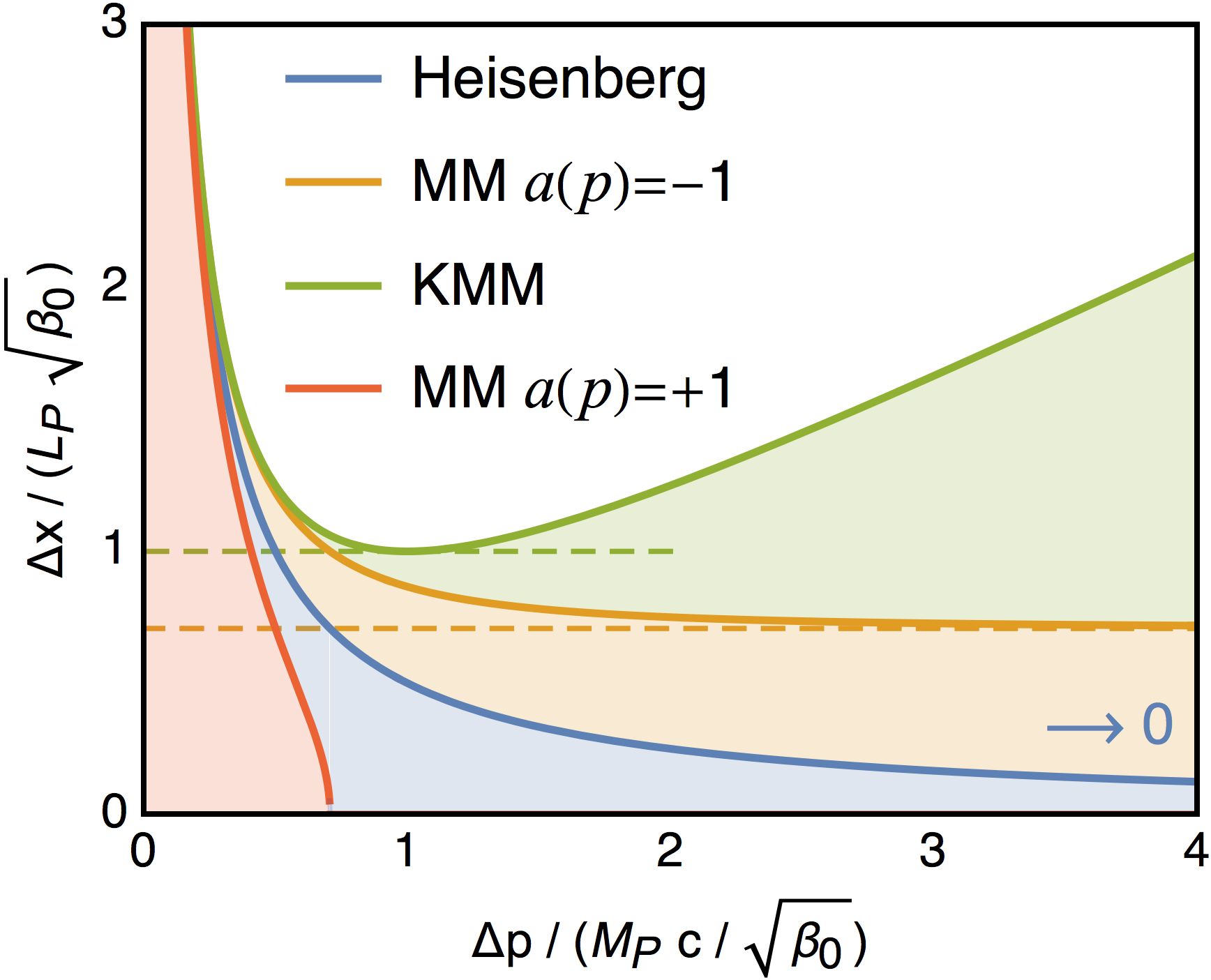
Figure 1: Bound on $\Delta x$ as a function of $\Delta p$ for different uncertainty principles. Blue: the Heisenberg uncertainty relation allows for arbitrarily small $\Delta x$ as $\Delta p$ increases. Orange: the MM GUP Eq. (25) obtained from Eq. (20) predicts a minimum $\Delta x$ for large $\Delta p$. Green: the KMM GUP Eq. (31) obtained from Eq. (30) predicts a minimum $\Delta x$ for a finite $\Delta p$, after which the position uncertainty increases again. Red: the other MM GUP obtained from Eq. (37), which can be associated to a quantum-to-classical transition where $[x_{i},p_{j}]=0$ when $\Delta p$ is larger than a critical value. Shaded regions are regions excluded by the corresponding uncertainty relation.

III Generalized uncertainty principle and quantum-to-classical transition

We now turn the attention to the solution of Eqs. (5) and (6) obtained by setting $a(p)=+1$. In this case, Eq. (7) becomes

$$f(p)=\sqrt{\alpha-\frac{p^{2}}{\kappa^{2}c^{2}}}\;.$$ (34)

With the choice of integration constant $\alpha=1$, we have

$$\left[x_{i},x_{j}\right] = \left(\frac{\hbar}{\kappa c}\right)^{2}\,i\epsilon_{ijk}J_{k}\;,$$ (35)

$$\left[x_{i},p_{j}\right] = i\hbar\,\delta_{ij}\,\sqrt{1-\frac{p^{2}}{\kappa^{2}c^{2}}}\;.$$ (36)

Similarly, with the choice of integration constant analogous to that leading to Eq. (12), we get

$$\left[x_{i},p_{j}\right]=i\hbar\,\delta_{ij}\,\sqrt{1-\frac{E^{2}}{\kappa^{2}c^{4}}}\;.$$ (37)

This solution is intriguing. Since the square root on the right-hand side is a decreasing function of momentum (always smaller than one), it no longer produces a term in the uncertainty principle that induces a minimum observable length, which was the initial motivation of these investigations. Rather, it describes a situation in which a system becomes more and more classical as its momentum (or its energy) approaches a critical value, of the order of the Planck scale, where eventually the commutator vanishes. Beyond this energy, one can then simply set $[x_{i},p_{j}]=0$, by continuity. Note that, if set $f(p)=0$ for $p$ larger than the critical value $\kappa c$ [or for $E$ larger than the critical value $\kappa c^{2}$, if we use Eq. (37)], Eq. (6) also implies $a(p)=0$ for $p>\kappa c$ (or, respectively, $E>\kappa c^{2}$), so the geometry becomes commutative. It therefore describes a sort of quantum-to-classical transition, in which, beyond a critical energy or momentum, the $[x,p]$ commutator vanishes (see Fig. 1, red line), and also $[x_{i},x_{j}]=0$.

For $E$ smaller than $\kappa c^{2}$, but close to it, Eq. (37) becomes

$$\left[x_{i},p_{j}\right]\simeq i\hbar\,\delta_{ij}\,\sqrt{2}\,\left(1-\frac{E}{\kappa c^{2}}\right)^{1/2}\;.$$ (38)

The energy dependence on the right-hand side has the typical form of the behavior of an order parameter at a second order phase transition, with a critical index equal to $1/2$. The prototype example of this is the magnetization as a function of the temperature in the Ising model, which, in the mean field approximation, is given by

$$M(T)\simeq M_{0}\left(1-\frac{T}{T_{c}}\right)^{1/2}\;.$$ (39)

Note also that, contrary to some interpretation in the literature, an equation such as Eq. (36) or Eq. (37) does not necessarily imply the existence of a maximum momentum, since the commutator can just be set to zero by continuity above the critical value. This is similar to the fact that Eq. (39) does not imply the existence of a maximum temperature for the Ising model; but simply that $M(T)=0$ for $T>T_{c}$.

IV Algebraic GUP and time discretization at the Planck scale

The algebraic formulation of the GUP given in Eqs. (8) and (12), as well as that in Eqs. (35) and (37), has an interesting relation with deformations of the Poincaré algebra, and to a discretization of time at the Planck scale Maggiore:1993zu . We review this idea here, following the discussion presented in Ref. Maggiore:2002qr .

IV.1 Discretized spatial dimensions and deformed Poincaré symmetry

Let us begin by considering a 1+1 dimensional system with a continuous time variable, while space is discretized on a regular lattice, with lattice spacing $d$. A wave equation, such as a Klein-Gordon equation, becomes in this framework (setting, for simplicity, $\hbar=c=1$ in the intermediate steps)

$$\left(-\frac{1}{c^{2}}\partial_{t}^{2}+\Delta_{x}^{2}-m^{2}\right)\phi=0\;,$$ (40)

where

$$\Delta_{x}\phi(t,x)=\frac{\phi(t,x+d)-\phi(t,x-d)}{2d}$$ (41)

is a discretization of the spatial derivative. The dispersion relation that follows is

$${\cal E}^{2}=\frac{\sin^{2}(d\,p)}{d^{2}}+m^{2}\;.$$ (42)

Momentum is periodically identified, and there is a maximum energy that can be carried by a wave solution, ${\cal E}_{\rm max}=(d^{-2}+m^{2})^{1/2}$. If we replace the speed of light $c$ (that here we have set to unity) by a speed $v<1$, this equation describes the propagation of phonons in $1+1$ dimensions.

A system described by Eq. (40) has an underlying Lie algebra with two symmetry generators: the generator $H$ of continuous time translations and the generator $P$ of discrete spatial translations, satisfying the Lie algebra $[H,P]=0$, supplemented by the identification $P\sim P+2\pi/d$. The symmetry under boosts is broken, and no generator is associated to it. However, it was observed long ago Bonechi:1992qf that this system has an alternative description in terms of a deformed algebra: one introduces also the boost generator $K$, and considers the algebra

$$\left[P,H\right] =0\,,\hskip 28.45274pt\left[K,P\right]=iH\,,$$ (44)

$$\left[K,H\right]=i\,\frac{\sin(2dP)}{2d}\;.$$

In the limit $d\rightarrow 0$ this reduces to the Poincaré algebra of a 1+1 continuous relativistic system. The algebra given by Eqs. (44) and (44), however, is well defined also at finite $d$, since the commutators obey the Jacobi identities. Eqs. (44, 44) provide an example of a deformed algebra, in which $d$ is the deformation parameter. Its relevance, in connection with a system described by Eq. (40), is that this deformed algebra has a quadratic Casimir $C_{2}$ given by

$$C_{2}=H^{2}-\frac{\sin^{2}(dP)}{d^{2}}\;,$$ (45)

Therefore, the dispersion relation (42) is simply the condition $C_{2}=m^{2}$, and in this sense this deformed Poincaré algebra can be considered as the symmetry of a relativistic system living in discrete one-dimensional space and continuous time.

Comparing the Lie algebra and the deformed algebra descriptions of the symmetries in this system we see that, in the Lie algebra approach, when $d\neq 0$, there are only two generators, $H$ and $P$; $d=0$ is a point of enhanced symmetry, where a new symmetry transformation, boosts, emerges, and the corresponding generator $K$ suddenly appears. In the deformed algebra description, instead, we always have a description in terms of three generators $H,P,K$ even for finite $d$, but we pay this with a non-linear structure. The value $d=0$ is a special point at which this algebraic structure linearizes.

IV.2 Discreteness of time and the algebraic GUP

Consider next a system in which time is discrete, in steps of size $\tau$, and space is continuous. We begin with $1+1$ dimensions, and we consider the equation (still setting for the time being $\hbar=c=1$)

$$(-\Delta_{t}^{2}+\partial_{x}^{2}-m^{2})\phi=0\;,$$ (46)

where

$$\Delta_{t}\phi(t,x)=\frac{\phi(t+\tau,x)-\phi(t-\tau,x)}{2\tau}\;,$$ (47)

and $\tau$ is the discrete time step. The corresponding dispersion relation is

$$\frac{\sin^{2}\tau{\cal E}}{\tau^{2}}=p^{2}+m^{2}\;.$$ (48)

We can find a quantum algebra description of this system, just by exchanging the role of $H$ and $P$ in Eqs. (44) and (44), and replacing the spatial step $d$ with the temporal step $\tau$,

$$\left[P,H\right] =0\,,\hskip 28.45274pt\left[K,H\right]=iP\;,$$ (50)

$$\left[K,P\right]=i\,\frac{\sin(2\tau H)}{2\tau}\;.$$

The quadratic Casimir operator of this algebra is

$$C_{2}=\frac{\sin^{2}(\tau H)}{\tau^{2}}-P^{2}\;.$$ (51)

so the dispersion relation (48) corresponds again to the condition $C_{2}=m^{2}$, with ${\cal E}$ identified with the eigenvalue of the operator $P^{0}$ and $p$ with the eigenvalue of the operator $P$.

The above construction can be generalized to the case of discrete time and more continuous spatial dimensions. Indeed, Eqs. (50) and (50) are just the restriction to $1+1$ dimensions of the $\kappa$-deformed Poincaré algebra, a deformation of the Poincaré algebra that can be written in any number of dimensions as it follows Lukierski:1991 ; Lukierski:1992dt . All commutators involving the angular momentum $J_{ij}$ are the same as in the undeformed Poincaré algebra. Hence, the group of spatial rotations is not deformed. Similarly, for space-time translations still holds $[P_{\mu},P_{\nu}]=0$. The commutators involving the boosts $K_{i}=J_{i0}$ are instead

$$\left[K_{i},H\right]=iP_{i}\,,\hskip 14.22636pt[K_{i},P_{j}]=i\delta_{ij}\frac{\sin(2\tau H)}{2\tau}\;,$$ (52)

and

$$\left[K_{i},K_{j}\right] = -iJ_{ij}\cos(2\tau H)$$ (53)

$$-i\tau^{2}P^{k}(P_{i}J_{jk}+P_{j}J_{ki}+P_{k}J_{ij})\;.$$

The quadratic Casimir is

$$C_{2}=\frac{\sin^{2}(\tau H)}{\tau^{2}}-{\bf P}^{2}\;,$$ (54)

and therefore $C_{2}=m^{2}$ gives

$$\frac{\sin^{2}\tau{\cal E}}{\tau^{2}}={\bf p}^{2}+m^{2}\;.$$ (55)

The relation between the $\kappa$-deformed Poincaré algebra and the algebraic formulation of the GUP emerges in the following way Maggiore:1993zu ; Maggiore:2002qr . In standard quantum mechanics, we quantize a particle imposing

$$[x_{i},p_{j}]=i\delta_{ij}\;.$$ (56)

(Recall that we are temporarily setting $\hbar=1$. We will restore $\hbar$ and $c$ at the end). In momentum space the operator $x_{i}$ can then be represented as

$$x_{i}=i\,\frac{\partial}{\partial p_{i}}\;,$$ (57)

and the velocity of the particle in the Heisenberg representation is given by

$$\dot{x}_{i}=i\,[H,x_{i}]=\frac{\partial{\cal E}}{\partial p_{i}}\;.$$ (58)

For the case of a discretized spatial dimension, discussed in section IV.1, using Eq. (42) (and setting for simplicity $m=0$) gives

$$\frac{\partial{\cal E}}{\partial p_{i}}=\hat{p}_{i}\cos(ap)\;,$$ (59)

where $\hat{p}_{i}$ is the unit vector in the direction of ${\bf p}$. This is the standard result for the group velocity of a massless particle on a regular spatial lattice.

However, the same procedure applied to the case of a discrete time dimension gives immediately a puzzling result. If we assume the validity of Eq. (56), and therefore of Eq. (57), using Eq. (55) we get

$$v_{i}=\frac{\partial{\cal E}}{\partial p_{i}}=\left(\frac{p_{i}}{\sqrt{p^{2}+m^{2}}}\right)\,\frac{1}{\cos(\tau{\cal E})}\;.$$ (60)

The term in parenthesis is just the standard expression for the velocity in terms of momentum. However, the cosine at the denominator makes no sense, and if we take Eq. (60) as an expression for the velocity, we find that $v>1$, and even diverges when $\tau{\cal E}$ approaches $\pi/2$.

Clearly, Eq. (57) cannot be the correct expression for the position operator when time is discrete and the dispersion relation has the form (55). Rather, a natural approach is to define the position operator requiring that the relation between velocity and momentum, $v_{i}=p_{i}/\sqrt{p^{2}+m^{2}}$, stays unchanged, so that, in particular, $v$ increases monotonically from zero to the speed of light (that we have set here to one) as momentum ranges from zero to infinity. This can be obtained defining, in momentum space,

$$x_{i}=i\cos(\tau{\cal E})\frac{\partial}{\partial p_{i}}\;.$$ (61)

By construction we now have

$$v_{i}=i[H,x_{i}]=\cos(\tau{\cal E})\frac{\partial{\cal E}}{\partial p_{i}}=\frac{p_{i}}{\sqrt{p^{2}+m^{2}}}\;.$$ (62)

Then, using Eq. (61), we can compute explicitly the $[x_{i},x_{j}]$ and $[x_{i},p_{j}]$ commutators, and we find (restoring the correct powers of $\hbar$ and $c$)

$$\left[x_{i},x_{j}\right] = i(c\tau)^{2}J_{ij}\,,$$ (63)

$$\left[x_{i},p_{j}\right] = i\hbar\delta_{ij}\,\sqrt{1-\frac{\tau^{2}}{\hbar^{2}}({\bf p}^{2}c^{2}+m^{2}c^{4})}\;,$$ (64)

where we have defined

$$J_{ij}=-i\left(p_{i}\frac{\partial}{\partial p_{j}}-p_{j}\frac{\partial}{\partial p_{i}}\right)\;.$$ (65)

We thus recovered the modified algebra given in Eqs. (35) and (37), with the identification $\tau=\hbar/(\kappa c^{2})$.

This result is quite remarkable. It shows that the GUP given by Eqs. (35) and (37) [which, apart from a choice of integration constant, is one of the only two possible expressions fixed by algebraic arguments, once one correctly takes into account that Eq. (5) requires $da/dp=0$ in order for the argument to be valid for particles with arbitrary spin] has an intriguing physical interpretation as the natural form of the uncertainty principle when the time variable becomes discrete at the Planck scale. Therefore, a discretization of time at the Planck scale implies that a system becomes classical as its energy approaches the Planck energy, since there the commutator $[x_{i},p_{j}]$ vanishes.

We can now ask what setting corresponds to the other allowed form of the algebraic uncertainty principle, given by Eqs. (8) and (12). As discussed in Ref. Maggiore:2002qr , this GUP emerges automatically when we start from an euclidean KG equation (here for simplicity in one spatial dimension)

$$(\Delta_{t}^{2}+\partial_{x}^{2}-m^{2})\phi=0\;.$$ (66)

The corresponding dispersion relation is

$$-\frac{\sin^{2}\tau{\cal E}}{\tau^{2}}=p^{2}+m^{2}\;.$$ (67)

We then perform a Wick rotation back to Minkowski space, which is equivalent to transforming ${\cal E}\rightarrow-i{\cal E}$, and the dispersion relation becomes

$$\frac{\sinh^{2}\tau E}{\tau^{2}}=p^{2}+m^{2}\;.$$ (68)

Formally Eqs. (48) and (68) are related by $\tau\rightarrow i\tau$. Substituting $\tau\rightarrow i\tau$ into Eqs. (50) and (50) we therefore find a deformation of the Poincaré algebra whose Casimir reproduces the dispersion relation (68),

$$\left[P,H\right] =0\,,\hskip 28.45274pt\left[K,H\right]=iP\;,$$ (70)

$$\left[K,P\right]=i\,\frac{\sinh(2\tau H)}{2\tau}\;.$$

This algebra can be generalized to more spatial dimensions, and it is the other version of the $\kappa$-Poincaré algebra found in Lukierski:1992dt ; Lukierski:1993wxa . The deformed commutators are

$$[K_{i},H]=iP_{i}\,,\hskip 14.22636pt[K_{i},P_{j}]=i\delta_{ij}\frac{\sinh(2\tau H)}{2\tau}\;,$$ (71)

$$[K_{i},K_{j}] = -iJ_{ij}\cosh(2\tau H)$$ (72)

$$+i\tau^{2}P^{k}(P_{i}J_{jk}+P_{j}J_{ki}+P_{k}J_{ij})\;,$$

with all other commutators undeformed, and the quadratic Casimir

$$C_{2}=\frac{\sinh^{2}(\tau H)}{\tau^{2}}-{\bf P}^{2}\;.$$ (73)

In this case, proceeding as above, one realizes that the correct definition of the position operator is Maggiore:1993zu ; Maggiore:2002qr

$$x_{i}=i\cosh(\tau E)\frac{\partial}{\partial p_{i}}$$ (74)

and, computing the $[x_{i},x_{j}]$ and $[x_{i},p_{j}]$ commutators, one finds the GUP in the form given in Eqs. (8) and (12).

V GUP for composite systems

A well-know problem concerning the GUP is how to extend it from microscopic degrees of freedom to composite objects and, eventually, to macroscopic objects. The non-linearity of the GUP commutators implies that the commutator obeyed by the center of mass position and total momentum of a composite object is not the same as that of the fundamental constituents (see below). A first question, then, is to what ‘fundamental’ constituents the GUP, in any of the forms discussed above, is supposed to apply. If the GUP emerges from a fundamental theory of gravity, it is natural to assume that it will apply to the elementary excitations of that theory. The next issue is what happens to composite systems and, in particular, to macroscopic objects. In the realm of elementary particles, terms such as $E^{2}/(\kappa^{2}c^{4})$ in eqs. (12) or (37) represent small corrections, if we take $\kappa$ of order of $M_{\rm P}$, and $E\ll M_{\rm P}c^{2}$. However, for macroscopic objects, these terms are huge. The Planck mass correspond to about $10^{-5}\,{\rm gr}$, so for a macroscopic object of mass $m$ even $m/\kappa$ can be large. Naively, this seems to imply that GUP effects become very large for macroscopic objects. This, however, is not necessarily the case, as it was shown in Amelino-Camelia:2013fxa (see also the Supplementary material in Pikovski:2011zk ) for the KMM form of the GUP. The argument is as follows. Consider a macroscopic body made of $N$ particles, taken for simplicity to have all the same mass, and labeled by an index $\alpha=1,\ldots,N$, with coordinates $x^{i}_{\alpha}$ and momenta $p^{i}_{\alpha}$. The center of mass coordinates $X^{i}$ and the total momentum $P^{i}$ of the composite system are defined as

$$X^{i}=\frac{1}{N}\sum_{\alpha=1}^{N}x^{i}_{\alpha}\,,\qquad P^{i}=\sum_{\alpha=1}^{N}p^{i}_{\alpha}\,.$$ (75)

Assuming a GUP of the form (18) with $F(p^{2})=\beta p^{2}$, we have

$$\left[x^{i}_{\alpha},p^{j}_{\alpha^{\prime}}\right]=i\hbar\delta^{ij}\,\delta_{\alpha\alpha^{\prime}}(1+\beta p_{\alpha}^{2})\,.$$ (76)

Then

$$\left[X^{i},P^{j}\right] = \frac{1}{N}\sum_{\alpha=1}^{N}\sum_{\alpha^{\prime}=1}^{N}\,\left[x^{i}_{\alpha},p^{j}_{\alpha^{\prime}}\right]$$ (77)

$$= i\hbar\delta^{ij}\frac{1}{N}\sum_{\alpha=1}^{N}\,(1+\beta p_{\alpha}^{2})$$

$$= i\hbar\delta^{ij}\left[1+\frac{\beta}{N}\sum_{\alpha,\beta=1}^{N}p_{\alpha}^{2}\right]\,.$$

For an object moving in an quasi-rigid manner, in order of magnitude $p_{\alpha}\sim P/N$, where $P$ is the modulus of the total momentum, and therefore

$$\left[X^{i},P^{j}\right]=i\hbar\delta^{ij}\left[1+{\cal O}(\frac{\beta P^{2}}{N^{2}})\right]\,.$$ (78)

Therefore, for a macroscopic object, $\beta$ in Eq. (76) has been replaced by $\beta/N^{2}$ and, for $N$ of the order of the number of constituent of a macroscopic object, this quantity is utterly negligible. More precisely, Eq. (77) can be rewritten as Amelino-Camelia:2013fxa

$$\left[X^{i},P^{j}\right]=i\hbar\delta^{ij}\left[1+\frac{\beta P^{2}}{N^{2}}+\frac{\beta}{N}\sum_{\alpha,\beta=1}^{N}\left(p_{\alpha}^{2}-\frac{P^{2}}{N^{2}}\right)\right]\,.$$ (79)

The last term is the variance of $p_{\alpha}^{2}$, multiplied by $\beta/N$, and vanishes for an exactly rigid body. For non-rigid objects, depending on the details of the internal structure, one could hope that the variance leaves, overall, an effect that scales as $(\beta P^{2}/N^{\alpha})$, with $\alpha$ a power in the range $0<\alpha<2$ Kumar:2019bnd . In any case, the effect of the GUP appears to be strongly suppressed for macroscopic objects.

Essentially the same derivation can be adapted to the GUP in the forms (9) or (36) [or in the forms written in terms of energy, Eqs. (12) and (37)]. Using for definiteness Eq. (20), expanding the square root as in Eq. (22) and replacing $p_{\alpha}=P/N$ for an exactly rigid object, we get

$$\left[X^{i},P^{j}\right] = i\hbar\delta^{ij}\frac{1}{N}\sum_{\alpha=1}^{N}\,\sqrt{1+2\beta p_{\alpha}^{2}}$$ (80)

$$= i\hbar\delta^{ij}\,\frac{1}{N}\sum_{\alpha=1}^{N}\,\sum_{n=0}^{\infty}c_{n}(2\beta p_{\alpha}^{2})^{n}$$

$$= i\hbar\delta^{ij}\,\frac{1}{N}\sum_{\alpha=1}^{N}\,\sum_{n=0}^{\infty}c_{n}(2\beta P^{2}/N^{2})^{n}$$

$$= i\hbar\delta^{ij}\,\sqrt{1+\frac{2\beta P^{2}}{N^{2}}}\;.$$

In summary, if the GUP applies to the constituents particles of a rigid macroscopic body, the same form of the modified commutator applies to the center of mass position and momentum with a rescaling $\beta\rightarrow\beta/N^{2}$.

VI Further extensions of the algebraic structure

When discussing the consequences of a GUP, one should not forget that the structure of the commutators is only one side of the aspect, and the dynamics, e.g. the form of the Hamiltonian, is another. These two are tied together by the possibility of redefining variables. Consider, for instance, a one-dimensional system, characterized by a commutator of the form

$$[x,p]=i\hbar f(p)\,.$$ (81)

In momentum space, the operator $x$ can be represented as

$$x\rightarrow i\hbar f(p)\frac{\partial}{\partial p}\,.$$ (82)

Then, defining $k(p)$ from requiring

$$f(p)\frac{dk}{dp}=1\,,$$ (83)

at the corresponding operator level we get the canonical commutator

$$[x,k]=i\hbar f(p)\frac{\partial}{\partial p}k=i\hbar\,.$$ (84)

From the point of view of the dynamics, consider the Hamiltonian of the system to be

$$H[x,p]=\frac{p^{2}}{2m}+V(x)\;.$$ (85)

In terms of the $(x,p)$ variables we have a ‘normal’ Hamiltonian, but a deformed commutator (81). On the other hand, if we rather use the variables $(x,k)$ we have a canonical commutation relation (84), at a price of a modified Hamiltonian

$$H[x,k]=\frac{p^{2}(k)}{2m}+V(x)\;.$$ (86)

For a general function $f(p)$, $H[x,k]$ contains arbitrarily high powers of $k$ and therefore, in coordinate space, contains spatial derivatives of arbitrarily high order [i.e., it is non-local, in the field-theoretical sense].

Note however that, if we take as Hamiltonian

$$H=\frac{k^{2}(p)}{2m}+V(x)$$ (87)

in terms of the $(x,p)$ variables, this would look as a very complicated quantum system described by deformed commutation relations and nonlocal Hamiltonian; even if, once one passes to the $(x,k)$ variables, one realizes that this is just a normal quantum system, with a standard local Hamiltonian and canonical commutation relation. This trivial example shows that the algebraic structure of the commutation relations is only one side of the coin, and must always be examined together with the dynamics of the system (see also the discussion in Pedram:2011aa ; Hossenfelder:2012jw ).

The above example, where the commutator could be reduced to the underformed one, is however specific to a one-dimensional system. In more dimensions, in fact, the situation is more complex. First of all, one also has to consider the $[x_{i},x_{j}]$ commutator, which is non-trivial. Furthermore, there is also the possibility of adding a term $p_{i}p_{j}$ to the right-hand side of Eq. (3). The most general algebra consistent with rotational invariance is thus

$$\left[x_{i},x_{j}\right] = \left(\frac{\hbar}{\kappa c}\right)^{2}\,a(p)\,i\epsilon_{ijk}J_{k}\;,$$ (88)

$$\left[x_{i},p_{j}\right] = i\hbar\,\left[f(p)\delta_{ij}+g(p)p_{i}p_{j}\right]\;,$$ (89)

which depends on three functions $a(p)$, $f(p)$ and $g(p)$. In the momentum representation, the position operator can then be written as

$$x_{i}\rightarrow i\hbar\left[f(p)\frac{\partial}{\partial p_{i}}+g(p)p_{i}p_{k}\frac{\partial}{\partial p_{i}}\right]\,.$$ (90)

The non-trivial Jacobi identities now reduce to two differential equations for the three functions $a(p)$, $f(p)$ and $g(p)$, and these are no longer enough to find a unique solution (modulo a sign); rather, after imposing them, one remains with a solution parametrized by a free function.

However, consider the transformation to a new momentum variable of the form $k_{i}=u(p)p_{i}$, which is the most general transformation consistent with rotational invariance. Then, for the associated operators we get

$$[x_{i},k_{j}] = f(p)u(p)\delta_{ij}$$ (91)

$$+\left[\frac{u^{\prime}(p)}{p}\left(f(p)+g(p)p^{2}\right)+g(p)u(p)\right]p_{i}p_{j}\;.$$

We can then choose $u(p)$ so that the term proportional to $p_{i}p_{j}$ in Eq. (91) vanishes and, after renaming $f(p)u(p)$ as $f(p)$, we get back the structure in Eq. (4), with now $k_{i}$ as momentum variable. In this sense, one can always restrict to Eqs. (3) and (4), possibly at the price of nonlocal terms in the Hamiltonian, induced by the elimination of the term proportional to $p_{i}p_{j}$.

Alternatively, we can restrict the freedom by imposing $a(p)=0$. In this case we get $[x_{i},x_{j}]=0$, $[p_{i},p_{j}]=0$, and then the Jacobi identities fix the $[x_{i},p_{j}]$ commutator to Ali:2009zq ; Ali:2011fa

$$[x_{i},p_{j}]=i\hbar\,\left[\delta_{ij}(1-\alpha p+\alpha^{2}p^{2})+p_{i}p_{j}\left(-\frac{\alpha}{p}+3\alpha^{2}\right)\right]\;.$$ (92)

VII Conclusions

In this paper we have revisited some aspects of the algebraic approach to the generalized uncertainty principle and to deformations of the commutation relations. We have pointed out an important difference between the approaches by MM Maggiore:1993kv and by KMM Kempf:1994su , emphasizing that the KMM approach implicitly selects a branch of solution of the Jacobi identities that only holds for spin-zero particles, and hence cannot be representative of fundamental properties of space-time. In contrast, requiring, as in Maggiore:1993kv , that the algebraic formulation is consistent (in the sense of obeying the Jacobi identities) independently of the particle spin, provides a more fundamental approach, which also has some remarkable consequences. First, the algebraic structure becomes fixed, modulo a sign; in contrast to the KMM approach, where the $[x,p]$ commutator is an arbitrary function of momentum, which is then fixed on rather arbitrary grounds. Second, the two solutions that emerge (in correspondence with the two possible signs) describe quite different physics; one gives a GUP with a minimum length uncertainty of the type found in string theory or with Gedanken experiment with black holes; the other describes a system that, near the Planck scale, becomes classical. Moreover, these two solutions have a very intriguing interpretation, namely as the natural commutation relations obtained in theories where time becomes discrete at the Planck scale. The two different solutions emerge, in this context, either discretizing directly Minkowski time, or discretizing time in the Euclidean formulation, and then rotating back to Minkowski space.

Finally, we have also re-examined, in our context, the issue of GUP for composite system, confirming the conclusion that the GUP does not extend trivially to macroscopic objects. If the deformed commutator is applied at the level of the constituent particles, then its effects are suppressed by powers of the number of constituents, thus suggesting that the effects of GUP will be limited to the realm of elementary particles with Planckian energies.

Acknowledgments. We thank Igor Pikovski and Yiwen Chu for useful discussions. MF was supported by The Branco Weiss Fellowship – Society in Science, administered by the ETH Zürich. The work of MM is supported by the Swiss National Science Foundation and by the SwissMap National Center for Competence in Research.

References

- (1) G. Veneziano, “A Stringy Nature Needs Just Two Constants,” Europhys. Lett. 2 (1986) 199.
- (2) D. Amati, M. Ciafaloni, and G. Veneziano, “Superstring Collisions at Planckian Energies,” Phys. Lett. B 197 (1987) 81.
- (3) D. Amati, M. Ciafaloni, and G. Veneziano, “Can Space-Time Be Probed Below the String Size?,” Phys. Lett. B 216 (1989) 41–47.
- (4) D. J. Gross and P. F. Mende, “The High-Energy Behavior of String Scattering Amplitudes,” Phys. Lett. B 197 (1987) 129–134.
- (5) D. J. Gross and P. F. Mende, “String Theory Beyond the Planck Scale,” Nucl. Phys. B 303 (1988) 407–454.
- (6) M. Maggiore, “A Generalized uncertainty principle in quantum gravity,” Phys. Lett. B 304 (1993) 65–69, arXiv:hep-th/9301067.
- (7) R. J. Adler and D. I. Santiago, “On gravity and the uncertainty principle,” Mod. Phys. Lett. A 14 (1999) 1371, arXiv:gr-qc/9904026.
- (8) S. Hossenfelder, “Minimal Length Scale Scenarios for Quantum Gravity,” Living Rev. Rel. 16 (2013) 2, arXiv:1203.6191 [gr-qc].
- (9) A. Hagar, Discrete or Continuous? The Quest for Fundamental Length in Modern Physics. Cambridge University Press, 2014.
- (10) M. Maggiore, “The Algebraic structure of the generalized uncertainty principle,” Phys. Lett. B 319 (1993) 83–86, arXiv:hep-th/9309034.
- (11) M. Maggiore, “Quantum groups, gravity and the generalized uncertainty principle,” Phys. Rev. D 49 (1994) 5182–5187, arXiv:hep-th/9305163.
- (12) A. Kempf, G. Mangano, and R. B. Mann, “Hilbert space representation of the minimal length uncertainty relation,” Phys. Rev. D 52 (1995) 1108–1118, arXiv:hep-th/9412167.
- (13) M. Maggiore, “The Atick-Witten free energy, closed tachyon condensation and deformed Poincaré symmetry,” Nucl. Phys. B 647 (2002) 69–100, arXiv:hep-th/0205014.
- (14) G. Amelino-Camelia, “Challenge to Macroscopic Probes of Quantum Spacetime Based on Noncommutative Geometry,” Phys. Rev. Lett. 111 (2013) 101301, arXiv:1304.7271 [gr-qc].
- (15) K. Nouicer, “Quantum-corrected black hole thermodynamics to all orders in the Planck length,” Phys. Lett. B 646 (2007) 63–71, arXiv:0704.1261 [gr-qc].
- (16) P. Pedram, “A Higher Order GUP with Minimal Length Uncertainty and Maximal Momentum,” Phys. Lett. B 714 (2012) 317–323, arXiv:1110.2999 [hep-th].
- (17) W. S. Chung and H. Hassanabadi, “A new higher order GUP: one dimensional quantum system,” Eur. Phys. J. C 79 no. 3, (2019) 213.
- (18) L. Petruzziello, “Generalized uncertainty principle with maximal observable momentum and no minimal length indeterminacy,” Class. Quant. Grav. 38 no. 13, (2021) 135005, arXiv:2010.05896 [hep-th].
- (19) J. Magueijo and L. Smolin, “Generalized Lorentz invariance with an invariant energy scale,” Phys. Rev. D 67 (2003) 044017, arXiv:gr-qc/0207085.
- (20) P. Jizba, H. Kleinert, and F. Scardigli, “Uncertainty Relation on World Crystal and its Applications to Micro Black Holes,” Phys. Rev. D 81 (2010) 084030, arXiv:0912.2253 [hep-th].
- (21) F. Bonechi, E. Celeghini, R. Giachetti, E. Sorace, and M. Tarlini, “Inhomogeneous quantum groups as symmetries of phonons,” Phys. Rev. Lett. 68 (1992) 3718–3720, arXiv:hep-th/9201002.
- (22) J. Lukierski, H. Ruegg, A. Nowicki, and V. Tolstoy, “q-deformation of Poincaré algebra,” Phys. Lett. B 264 (1991) 331.
- (23) J. Lukierski, A. Nowicki, and H. Ruegg, “New quantum Poincare algebra and k deformed field theory,” Phys. Lett. B 293 (1992) 344–352.
- (24) J. Lukierski and H. Ruegg, “Quantum kappa Poincare in any dimension,” Phys. Lett. B 329 (1994) 189–194, arXiv:hep-th/9310117.
- (25) I. Pikovski, M. R. Vanner, M. Aspelmeyer, M. S. Kim, and C. Brukner, “Probing Planck-scale physics with quantum optics,” Nature Phys. 8 (2012) 393–397, arXiv:1111.1979 [quant-ph].
- (26) S. P. Kumar and M. B. Plenio, “On Quantum Gravity Tests with Composite Particles,” Nature Commun. 11 no. 1, (2020) 3900, arXiv:1908.11164 [quant-ph].
- (27) P. Pedram, “New Approach to Nonperturbative Quantum Mechanics with Minimal Length Uncertainty,” Phys. Rev. D 85 (2012) 024016, arXiv:1112.2327 [hep-th].
- (28) A. F. Ali, S. Das, and E. C. Vagenas, “Discreteness of Space from the Generalized Uncertainty Principle,” Phys. Lett. B 678 (2009) 497–499, arXiv:0906.5396 [hep-th].
- (29) A. F. Ali, S. Das, and E. C. Vagenas, “A proposal for testing Quantum Gravity in the lab,” Phys. Rev. D 84 (2011) 044013, arXiv:1107.3164 [hep-th].