Comment on “Inferring broken detailed balance in the absence of observable currents”

Abstract

We present a simple biophysical example that invalidates the main conclusion of “Nat. Commun. 10, 3542 (2019)”. Moreover, we explain that systems with one or more hidden states between at least one pair of observed states that give rise to non-instantaneous transition paths between these states also invalidate the main conclusion of the aforementioned work. This provides a flexible roadmap for constructing counterexamples. We hope for this comment to raise awareness of possibly hidden transition paths and of the importance of considering the microscopic origin of emerging non-Markovian (or Markovian) dynamics for thermodynamics.

Ref. [1] entitled “Inferring broken detailed balance in the absence of observable currents” claims to derive a method which allows to identify an “underlying nonequilibrium process, even if no net current, flow, or drift, are present”. Below we explain that the above main result of said work, which is supposed to hold for semi-Markov processes, was in fact never tested by the authors, nor applied to an example. Remarkably, the central result of an older work by Wang and Qian [2] (cited in Ref. [50] in [1]) already disproves the main conclusion of Ref. [1] and, moreover, contains a recipe to construct counterexamples to the findings of Ref. [1].

The main result of Ref. [1] was never tested.— As the main result Ref. [1] derives Eq. (4) quantifying “irreversibility of stationary trajectories with zero current”, which is supposed to hold for semi-Markov processes [1] and is to be used to infer broken detailed balance. While the work contains two explicit examples, none of them in fact seems to apply to the main result. Instead, a variant of the main result (i.e. Eq. (6)) is derived, which provides a technique to identify irreversibility in certain second order semi-Markov processes, and is used in Figs. 2 and  3 of [1]. Notably, the authors use in Eqs. (4) and  (6) the same notation, which makes it difficult to actually notice that the main result (that is, Eq. (4)) was never applied to an example.

Counterexample.—Following [2] it is straightforward to construct an example that disproves the main conclusion of [1]. Consider a molecular motor that walks in two directions $x$ and $y$ “fueled” by a chemical reaction $\text{A}\rightleftharpoons\text{B}$. Along the $x$ direction the motor’s position $x_{t}$ at any time $t$ advances in a two step reaction

$$\mathrm{E}+\mathrm{A}+x_{t}\xrightleftharpoons[\kappa_{1}^{-}]{\kappa_{1}^{+}}\mathrm{EA}\xrightleftharpoons[\omega_{1}^{-}]{\omega_{1}^{+}}\mathrm{E}+\mathrm{B}+(x_{t}+1),$$ (1)

where “E” represents the enzymatic motor. The intermediate step – the formation of the complex “EA” – is assumed not to be visible or monitored (see dotted circles in Fig. 1(a)). Note that one could also consider a more complex enzyme with more unobserved intermediate enzymatic states. For simplicity and without loss of generality, we stick to this simple model. The motor’s position along the $y$ direction, $y_{t}$, evolves as a one-step process

$$\mathrm{E}+\mathrm{A}+y_{t}\xrightleftharpoons[\kappa_{2}^{-}]{\kappa_{2}^{+}}\mathrm{E}+\mathrm{B}+(y_{t}+1).$$ (2)

Whenever a molecule “A” is bound to the enzymatic motor we assume that the motor cannot be detected and the reaction (2) is switched off. For simplicity we set the rates equal to $\kappa_{1}^{\pm}=\omega_{1}^{\pm}=2$ and $\kappa_{2}^{\pm}=1$, tacitly assuming that all chemical species are kept at the same chemical potential, $\mu_{\rm A}=\mu_{\rm B}$. That is, the system satisfies detailed balance due to $\ln(\kappa_{1}^{+}/\kappa_{1}^{-})=\ln(\kappa_{2}^{+}/\kappa_{2}^{-})=\ln(\omega_{1}^{+}/\omega_{1}^{-})=0$ and the full dynamics is a Markov-jump process (see Fig. 1a). The last monitored position $z_{t}=(x_{t},y_{t})$ at any time $t$ becomes a semi-Markov process due to the hidden intermediate step in Eq. (1). The process $z_{t}$ thus satisfies all the assumptions that were made in Ref. [1] to derive the main result. Consequently, our example also satsfies Eq. (1) in Ref. [1]. Note that we refer to hidden states if they are unobserved. The number of unobserved states in general cannot be known. In the present example the reader only knows the number of hidden states because we describe the complete underlying mathematical model for the sake of reproducibility.

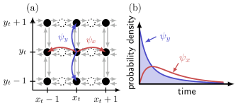
Figure 1: Motor moving in two dimensions. (a) The filled circles are the positions where we can observe the motor, whereas it cannot be detected in the dotted states. The last-visited observed node forms a semi-Markov process. (b) $\psi_{x}(t)$ and $\psi_{y}(t)$, the probability densities of the waiting time until the last-visited node changes in the $x$ and $y$ direction, respectively, given in Eq. (3).

The probabilities of the two reactions to be completed for the first time are equal, $p_{x,+}=p_{x,-}=p_{y,+}=p_{y,-}=1/4$, in both reactions. The turnover time until any of the two reactions is completed is distributed according to waiting time densities $\psi_{x,\pm}(t)$ and $\psi_{y,\pm}(t)$, which read

$$\psi_{x}(t) =\psi_{x,\pm}(t)=\frac{4}{3}\big{[}2{\rm e}^{-2t}-2{\rm e}^{-8t}\big{]},$$ (3)

$$\psi_{y}(t) =\psi_{y,\pm}(t)=\frac{4}{3}\big{[}{\rm e}^{-2t}+2{\rm e}^{-8t}\big{]}.$$

To obtain Eq. (3) we solve the conditional first passage problem in Fig. 1, where we use a filled circle as the starting point and impose absorbing boundaries on the filled circles adjacent to the starting point (see arrows in Fig. 1). In this particular case the time to leave a state in either $x$ or $y$ direction is actually exponential $\psi^{\rm exit}(t)\equiv\sum_{i\in\{x,y\}}[p_{i,+}+p_{i,-}]\psi_{i}(t)=2{\rm e}^{-2t}$ with mean exit time $\mathcal{T}\equiv\int_{0}^{\infty}t\psi^{\rm exit}(t)dt=1/2$. As shown in Fig. 1(b) we have $\psi_{x}(t)\neq\psi_{y}(t)$, that is, the waiting time densities are different and thus have a genuinely non-zero Kullback-Leibler divergence

$$D_{\rm KL}[\psi_{x}|\psi_{y}]\approx 0.28,\quad D_{\rm KL}[\psi_{y}|\psi_{x}]\approx 0.47,$$ (4)

respectively, where we have defined $D_{\rm KL}[\psi_{i}|\psi_{j}]\equiv\int_{0}^{\infty}\psi_{i}(t)\ln[\psi_{i}(t)/\psi_{j}(t)]dt$, where $i,j=x,y$. Using Eqs. (1) and (4) in [1] along with $D_{\rm KL}[\psi_{i}|\psi_{j}]\neq 0$ for $i\neq j$ one would mistakenly confuse this equilibrium system to be out of equilibrium. More precisely, Eq. (4) in [1] states that the entropy production of the waiting time is given by $\dot{S}_{\rm WTD}=\sum_{i,j,\alpha,\beta}p_{i,\alpha}p_{j,\beta}D_{\rm KL}[\psi_{i}|\psi_{j}]/\mathcal{T}\approx 2\times(0.28+0.47)=1.5>0$, where and $\alpha,\beta=\pm$; each term in the sum in fact is non-negative. The main result of Ref. [1] erroneously predicts this equilibrium system to break detailed balance (based on $\dot{S}_{\rm WTD}\neq 0$). Since our example clearly violates the main result of Ref. [1] while satisfying all the required assumptions, we have hereby disproved the main result in Ref. [1].

Opposing views on broken detailed balance.—A similar counterexample was sketched in an earlier work by Wang and Qian [2] who also stated in their abstract: “We show that for a semi-Markov process detailed balance is only a necessary condition, but not sufficient, for its time reversibility” [2]. In technical terms, Ref. [2] showed that if the waiting-time distribution to another state depends on the final state, the process becomes (mathematically) irreversible (here $\psi_{x}(t)\neq\psi_{y}(t)$) even if detailed balance is satisfied. Thus, $\psi_{x}(t)\neq\psi_{y}(t)$ must not be used as a signature of broken detailed balance as erroneously concluded in Ref. [1]. In light of these diametrically opposing views in [1] and [2] it is puzzling that Ref. [1] actually cites Ref. [2] as Reference [50].

Crucial elements of the counterexample.—Counterexamples to the main conclusion of [1] are obtained as soon as hidden states states (see dotted circles in Fig. 1a) emerge between at least one pair of observed states (see filled circles). This allows for passages over hidden states, called transition paths (see, e.g., [3]), to become non-instantaneous. In this case the coarse-graining must not commute with the time reversal – a phenomenon that we coined “kinetic hysteresis” which is an overdamped analogue of the odd parity of momenta [4]. We are not aware of any example without kinetic hysteresis which would allow for a non-vanishing waiting-time entropy production, i.e. $\dot{S}_{\rm WTD}\neq 0$, for a semi-Markov process. For example, in absence of hidden cycles at least one transition-path time must be non-vanishing to allow for the waiting-time distribution to couple to the state change [4] and in turn to allow for $\dot{S}_{\rm WTD}\neq 0$. Thus, if the transition paths become (effectively) instantaneous, the waiting time does not couple to the state change [4] (see [5] for a generalization that includes hidden cycles), i.e., $\dot{S}_{\rm WTD}=0$. These examples satisfying $\dot{S}_{\rm WTD}=0$ clearly cannot be used to infer “broken detailed balance in the absence of observable currents”, which was recently confirmed in Ref. [6] (see paragraph after Eq. (58) therein).

We emphasize that while our example proves the main conclusion of Ref. [1] to be false, we do not claim that all mathematical results in [1] are incorrect. In particular, we explicitly acknowledge that the compact expressions for the Kullback-Leibler divergence between two path measures indeed have some mathematical appeal (see also Ref. [7]). In other words Eq. (4) is mathematically sound it does not, however, allow to infer broken detailed balance. Moreover, whether a model in fact exists that upon coarse-graining yields a semi-Markov process and concurrently allows to infer broken detailed balance according to [1] remains an intriguing question.

Conclusion.— The authors never tested their main result Eq. (4), which is supposed to detect broken detailed balance. Here we presented an explicit model of a molecular motor that disproves this main conclusion of Ref. [1], which was in fact already invalidated earlier in Ref. [2] (Ref. [50] in [1]). Note that the example in Fig. 1 only formally disproves the variant of the main result in Eq. (6) in [1], which does hold for the more specialized semi-Markov processes of second order –processes with a waiting-time distribution that depends on the past and future states (see e.g. [1, 9, 10]). This variant thus allows to find examples for which it holds and thus potentially allows to infer “broken detailed balance in the absence of observable currents” [1, 9]. We hope that this comment raises awareness of the importance of considering the underlying dynamics from which possible non-Markovian (or Markovian) coarse-grained dynamics emerge.

Acknowledgments. The financial support from the German Research Foundation (DFG) through the Emmy Noether Program GO 2762/1-1 to A. G. is gratefully acknowledged.

References

- Martínez et al. [2019] I. A. Martínez, G. Bisker, J. M. Horowitz, and J. M. R. Parrondo, Nat. Commun. 10, 3542 (2019).
- Wang and Qian [2007] H. Wang and H. Qian, J. Math. Phys. 48, 013303 (2007).
- Makarov [2021] D. E. Makarov, J. Phys. Chem. B 125, 2467 (2021).
- Hartich and Godec [2021a] D. Hartich and A. Godec, Phys. Rev. X 11, 041047 (2021a).
- Ertel et al. [2021] B. Ertel, J. van der Meer, and U. Seifert, Operationally accessible uncertainty relations for thermodynamically consistent semi-Markov processes (2021), arXiv:2111.13113 .
- van der Meer et al. [2022] J. van der Meer, B. Ertel, and U. Seifert, Thermodynamic inference in partially accessible markov networks: A unifying perspective from transition-based waiting time distributions (2022). Accepted in Phys. Rev. X.
- Girardin and Limnios [2003] V. Girardin and N. Limnios, J. Appl. Prob. 40, 1060 (2003).
- Note [1] Note that we explicitly refer to semi-Markov processes (sMP) and not to possible generalizations to second- or higher order sMPs. However, any sMP is also a higher order sMP but the converse is untrue.
- Ehrich [2021] J. Ehrich, J. Stat. Mech. 2021, 083214 (2021).
- Hartich and Godec [2021b] D. Hartich and A. Godec, Violation of local detailed balance despite a clear time-scale separation (2021b), arXiv:2111.14734 .