figuret

This study was carried out at the Institute of Physics and Astronomy, Estonian Academy of Sciences.

The Dissertation was admitted on February 14, 1972, in partial fulfilment of the requirements for the degree of Doctor of Science in astronomy and celestial mechanics, and allowed for defence by the Council of the Institute of Physics, University of Tartu.

Opponents:	Prof. E. K. Kharadze
	Abastumani Observatory
	Georgia
	Prof. T. A. Agekian
	Leningrad University
	Russia
	Prof. G. M. Idlis
	Alma-Ata University
	Kazakstan
Leading institute: Lebedev Physical Institue of the Soviet Academy of Sciences.
Defence:	March 17, 1972, University of Tartu, Estonia

Original in Russian — I Volume: Chapters 1 – 7, 195 pages

II Volume: Chapters 8 – 23 with appendix, 330 pages

ISBN 978-9949-03-771-1

Copyright: Jaan Einasto, 2021

University of Tartu Press 2021

www.tyk.ee

Chapter 0 Preface to the English edition

The Thesis was an attempt to combine data from three previously independent areas: the structure and kinematics of stellar populations of the Galaxy, models of galaxies, and models of the evolution of galaxies. This synthesis was made with the goal to understand better the structure and evolution of galaxies. When the work was finished it was clear that there are difficulties and open problems in the classical picture. Thus, immediately after the Thesis was completed, I started together with my Tartu collaborators searching for solutions to open problems. This search led to accepting the presence of dark matter in galaxies. To understand the properties of dark matter in galaxies, it was needed to study the environment of galaxies and the distribution of galaxies in space, which culminated with the discovery of the cosmic web. A short overview of the development of ideas directly connected with the topic of the Thesis is given in the Epilogue.

In some sense the Thesis is a time-capsule of the state of affairs just at the verge of the paradigm shift in cosmology. The Thesis was written in Russian and its most important parts were never published. Thus, it would be useful to make this study available for the astronomical community by translating the Thesis into English.

According to Soviet rules, doctoral theses must be written in Russian and typed with a typewriter. It was common to base the thesis on previously published papers, thus these papers must be retyped to form a collection needed for the thesis. In early 1970’s, I had finished several cycles of papers on stellar kinematics and galactic models, suited as the basis of the Thesis. Also, I had unpublished results on the study of the dynamical and physical evolution of stellar systems. I prepared my Thesis on the basis of this work. About half of it was based on my papers published in Tartu Observatory Publications in Russian, and a few papers in English in conference proceedings. New results were written in 1971 as additional chapters of the Thesis. The text was typed only once with five carbon copies, all equations hand-written. Copies of better quality were given to thesis reviewers and to the Moscow office, where all theses completed in USSR were collected and revised for acceptance. The original copy of the Thesis in Russian is scanned and can be accessed in Dspace link: http://hdl.handle.net/10062/6113. The translated English version is available in link http://hdl.handle.net/10062/76090.

The Thesis consists of four parts, and is divided to 23 chapters. Chapters 4, 7, 20, 21, 22, 23 were unpublished and the present translation is their first publication. These chapters were translated in full. Chapters 7, 11, 17, 19 were published in Tartu Observatory Publications or conference proceedings, but form the methodical and data basis to understand the main topic of the Thesis, thus these chapters were also translated in full. The rest of chapters, published in Tartu Observatory Publications, describe the general background of the topic, and are written in this English version as short summaries of respective papers in Russian.

No original figures are available, only copies of very different quality from paper copies and microfilms to figures on typed pages of the Thesis. Copies were scanned and used to prepare figure files suitable for publication. Tables were partly retyped and partly scanned from the Thesis copy available.

The translation from Russian into English was made by myself, while my colleague Peeter Tenjes translated chapter 11. My grandson Peeter corrected figure files. My colleagues in Tartu Observatory helped to polish the text and to fix errors. The remaining errors are my own responsibility.

November 2021

Chapter 1 Preface

It is customary to divide the stellar astronomy into the theory of stellar systems and observational astronomy. The classical theory of stellar systems covers stellar dynamics and statistics, while observational astronomy covers direct information about the structure and composition of stellar systems and various astronomical and astrophysical methods of obtaining it.

Parenago (1948) introduced the concept of practical stellar dynamics to denote the study of the structure of stellar systems based on observational data with the application of theoretical relations, derived in the dynamics of stellar systems. Currently, the addition of stellar dynamics and other theoretical disciplines — theories of stellar evolution and chemical nucleosynthesis, gas dynamics, relativistic astrophysics, etc. — are also applied to the study of the structure of stellar systems. Retaining the convenient term of practical stellar dynamics, it is reasonable to accept for its goal the application of the results of the theory in the study of the structure and evolution of particular stellar systems.

The basic method of practical stellar dynamics is the construction of models of the objects under study. When considering theoretical problems, usually only a certain aspect of the model is essential, and there is no need to achieve representativeness of the model in other details, secondary to the problem. The goal of practical stellar dynamics is the developing of models of stellar systems, as representative as possible, in which the synthesis of heterogeneous observational information is based on the results of the theory of stellar systems.

The main tasks of practical stellar dynamics include the study of the evolution of stellar systems. The problem of evolution is considered primarily as an observational one, i.e. evolutionary conclusions are drawn on the basis of a theoretical interpretation of suitable observational data.

The body of works, which served as the basis for the present dissertation, is devoted to the development of methods of practical stellar dynamics and their application to investigate the structure and evolution of regular galaxies like our Galaxy. We did not set as a goal the further development of theory and obtaining new observational data, since the already available theoretical and observational information is much more than could be processed and combined in one cycle of studies.

The author’s interest in this subject arose already in the first half of the 1940s, when the author, being a young amateur astronomer, read with enthusiasm the articles by Ernst Öpik, Taavet Rootsmäe, Aksel Kipper and Grigori Kuzmin on the structure and evolution of stars and stellar systems in the pages of Calendars of Tartu Observatory. Here I would like to mention the pioneering works of Öpik (1938) and Rootsmäe (1961), which laid the foundation for revealing the relation between ages and kinematical and spatial properties of stellar populations in the Galaxy. The immediate impetus for beginning the research on practical stellar dynamics was received in 1951, when the author discussed with Pavel Parenago and Alla Massevich the possible topic for my diploma thesis. They suggested a detailed study of the kinematics of stars of the main sequence. Parenago (1951) had just discovered that the main sequence is kinematically inhomogeneous and wanted to have more detailed information on this effect. This problem was very close to my own interests as well as to the topic of the research of Prof. Rootsmäe, so I agreed. This resulted in my diploma thesis (Einasto 1952), as well as in my PhD thesis (Einasto 1954). From this work grew a series of studies on stellar kinematics, which served as the basis for the first section of the first part of the present Thesis.

In 1952 and 1955—1956 author performed calculations for models of the Galaxy by Kuzmin (1952a, 1956a). In the course of this work, I discovered that models can be refined by using some additional data that were not taken into account at that time. The idea of integrated use of observational information and theoretical results was later applied in developing the concept of a consistent system of local Galactic parameters and in constructing new empirical models of the Galaxy. The corresponding series of studies is included in the second section of the first part of the Thesis.

The construction of the Galactic model was hampered by two difficulties. First, the result strongly depends on the method of model building, in particular, on the choice of the initial description function. Second, due to our position inside the Galaxy, it is difficult to get a picture of its structure as a whole. To enrich our understanding of the global structure of the Galaxy, the study of other similar galaxies, among which Andromeda galaxy M31 is the most suitable, plays an essential role. Thus, two cycles of works arose, on the methods of building models of galaxies and on the study of the structure of the M31 galaxy, which form the content of the second and third parts of the dissertation.

Eggen et al. (1962) showed that we can draw certain conclusions about the evolution of the Galaxy from observational data on the spatial kinematical structure of subsystems of stars of different ages. The success of these authors prompted us to use the collected material to identify the possible evolutionary path of the Galaxy. In addition to the dynamical evolution, we also investigated the physical evolution, following the example of Tinsley (1968). The addition of the evolution issues allowed us to give the Thesis a more contemporary character.

Constructed models of our Galaxy and the Andromeda Galaxy are more detailed and representative than models known from the literature. However, the available observational possibilities to improve the models are far from being exhausted. On the other hand, the methodology developed can also be applied to study the structure and evolution of other galaxies.

Most of the results presented in the Thesis have been published. The relevant papers have been reproduced partly unchanged, partly in abridged or revised form. Some results obtained recently have not yet been published, so that the Thesis is of independent value. The arrangement of the material is generally chronological with some exceptions.

November 1971

Part 1 Spatial and kinematical structure of the Galaxy

Chapter 2 Kinematical structure of the main sequence

It is well known that the velocity distribution of stars has approximately the Schwarzschild character. The analysis of tangential velocities of main sequence stars has shown that stars of the early spectral type (hot giants) can be indeed presented by the Schwarzschild law (Einasto 1952, 1954). Stars of spectral classes F, G, K, M have velocity distributions, which can be presented as a sum of two Schwarzschild distributions with different velocity dispersions. A similar picture is observed in populations of giant stars. Non-homogeneity of kinematical characteristics of stellar populations is evidently caused by the large dispersion of population ages. Hot giant stars of main sequence are relatively young. In contrast, populations of stars of later spectral types of the main sequence as well as ordinary giant star populations are mixtures of stars of rather various ages.

In calculations of kinematical characteristics of stars, the selection of observational data is taken into account as well as the influence of random observational errors (Einasto 1955a). The Chapter is published by Einasto (1954), and is applied by Einasto (1955a, b), and Tiit & Einasto (1964).

Main results of the study can be summarised as follows.

1. A method is elaborated for treating the distribution of tangential velocities under the assumption that the sample consists of two groups of stars, with Schwarzschild velocity distributions with different dispersions. By comparing the observed and theoretical distributions of tangential velocities, the method makes it possible to determine these dispersions as well as the fractions of stars belonging to both groups. The position of the centroids and the ratio of the axes of the velocity ellipsoid were taken as given, since the distribution of tangential velocities was only weakly dependent on these parameters. In the method, the distorting effects are taken into account: errors in selection of proper motions, tangential velocity errors, and irregularities in the distribution of stars across the sky. The method also makes it possible to determine the average errors of the unknown quantities and to take into account the influence of possible errors in the given parameters. In addition, it is possible to calculate the mean variance of velocities corresponding to both groups of stars taken together.

2. The analysis of tangential velocities of main sequence stars in the spectral range from A5 to M leads to the following results. The distribution of velocities of A stars is well represented by a single Schwarzschild distribution. Starting from F stars, the observed velocity distribution can be represented as the sum of two Schwarzschild distributions with different dispersions: the stars are separated here statistically into two kinematical groups. The dispersions of velocities of both kinematical groups practically do not depend on the spectral type, but the fraction of stars with low velocities varies. It is minimal in spectral class G and increases towards the earlier and later spectral classes. In this connection the mean velocity dispersion (both kinematical groups taken together) is maximal at spectral class G and noticeably decreases in the transition to spectral F and A classes, as well as to K and M. Stars of the middle part of the main sequence can also be divided into two groups, however, the spectral division does not coincide with the kinematical one. The spectral separation is observed, firstly, only in the spectral range from F to G5. Secondly, the velocity dispersion of one spectrally separated group of stars coincides with the velocity dispersion of the first kinematical group (small velocities), while the velocity dispersion of the other group is much smaller than the dispersion of the second kinematical group (high velocities), and is close to the average dispersion in the second part of the main sequence.

3. The discrepancy between the spectral and kinematical separation is apparently due to the fact that only the spectral separation corresponds to the partitioning of the main sequence into two genetically unrelated parts, whereas the kinematical separation does not correspond to this division. The first part of the main sequence has a homogeneous kinematical structure and probably ends at the G5 spectral class. The second part of the main sequence starts at spectral class F and is characterised by a significant heterogeneity in the kinematical structure, with a possible continuous transition from stars with small velocity dispersion to stars with large velocity dispersion. The reason for the kinematical heterogeneity of the second part of the main sequence is most likely due to the difference in ages of the constituent stars. The youngest stars in the second part of the main sequence are red dwarfs with emission lines in their spectra and the lowest velocity dispersion. This allows us to conclude that velocities of stars of the second part of the main sequence increase with time.

1954

Chapter 3 Velocity dispersions from their observed velocities

In our recently published paper (Einasto 1954), we proposed a simple method of determining the velocity dispersion from the total tangential velocities of stars. The method is based on the fact that the mean value of the squared tangential velocity is proportional to the square of the velocity dispersion, if other parameters are identical. The formulas are given to calculate the coefficient of proportionality and to take into account the errors in parallax and the mean error of the dispersion. In a quite similar way, the mean velocity dispersion can be found from radial and total spatial velocities. For the proportionality coefficient velocities, a different expression is obtained than for the tangential velocities. The aim of the present work (Einasto 1955a) is to describe the method in more detail and to extend it to the case of radial and spatial velocities.

The advantage of this method is, first of all, that it is very easy to find the mean dispersion. The result is only very slightly dependent on the values of other parameters of velocity distributions. Another advantage of the method is that the calculation of the dispersion separately from radial and tangential velocities allows one to detect possible systematic errors in the material, for example, in stellar parallaxes. Finally, in this way of calculating the dispersion, it is very easy to account for observational errors in radial velocities, proper motions and parallaxes. Here we give a short summary of the paper.

The mean velocity dispersion of stellar populations can be calculated as follows:

$$\sigma^{2}=1/3(\sigma_{R}^{2}+\sigma_{\theta}^{2}+\sigma_{z}^{2}),$$ (1)

where $\sigma_{R}^{2}$, $\sigma_{\theta}^{2}$, $\sigma_{z}^{2}$ are velocity dispersions in cylindrical coordinates. The mean velocity dispersion is related to the mean observed velocity of stars, $V$:

$$\overline{V^{2}}=\beta\sigma^{2},$$ (2)

where $V$ is the stellar velocity from observations, and $\beta$ is a dimensionless coefficient, depending on the nature of $V$. As $V$ we can use the full spatial velocity of stars, $V_{s}$, tangential velocity, $V_{t}$, or radial velocity, $V_{r}$. Values of the coefficient $\beta$ are calculated for all these cases, using the generalised Kleiber theorem. The kinematics of Me dwarfs is studied using this method (Einasto 1955b).

The results obtained in this paper can be seen as a generalisation of the Kleiber theorem for moments of any order, including mixed moments, and for velocity distributions, which are not spherical. It is shown that the respective coefficients have in the case of arbitrary velocity distribution, including ellipsoidal, the same numerical values, as in the case of spherical velocity distribution, if stars are distributed uniformly over the whole sky, and if the velocity distribution function is the same in all regions of the sky. Since these conditions are in many cases well satisfied, one cannot agree with the occurrence in the literature the statement, that in the light of the modern understanding of velocity distributions, the Kleiber theorem has lost his meaning.

1955

Chapter 4 On the asymmetric shift of stellar velocity centroids

In this paper (Einasto 1961), we shall discuss one aspect of the velocity distribution – the asymmetric shift of the centroid of the velocity ellipsoid. A critical analysis of kinematical data, collected in the next Chapter, shows that only part of the available data can be used to study the asymmetric shift. Here we give a short summary of the paper.

For all populations we calculated the following data: the mean velocity dispersion,

$$\sigma=\sqrt{\frac{1}{3}(\sigma_{R}^{2}+\sigma_{\theta}^{2}+\sigma_{x}^{2})},$$ (1)

and the mean heliocentric centroid velocity in rotational direction, $\overline{V_{\theta}}$, where $\sigma_{R}$, $\sigma_{\theta}$, and $\sigma_{z}$ are velocity dispersions in galactic cylindrical coordinates. The velocity dispersions were corrected for observational errors using a method, proposed by us (Einasto 1955a). The age of populations was determined from Iben’s evolutionary tracks, see Chapters 4 and 22. For halo populations, the individual age determinations coincide within possible errors. The relative age of these populations was estimated theoretically, adopting for oldest halo populations the age of the Galaxy, $10^{10}$ yr, and for other halo populations an age needed for the population considered to collapse with free fall acceleration to its observed dimensions.

Figure 1: The Strömberg diagram for populations. In the horizontal axis, we show the heliocentric centroid velocity of the population in the direction of the Galactic rotation; in the vertical axis, we plot the mean velocity dispersion $\sigma=\sqrt{\frac{1}{3}(\sigma^{2}_{R}+\sigma^{2}_{\theta}+\sigma^{2}_{z})}$. Open circles are for metal-poor populations, dots for populations with normal metal abundance. The numbers give the birth-dates in $10^{9}$ years starting from the formation of the oldest populations, assuming for the age of the Galaxy $10^{10}$ years (Einasto 1974b).

The Strömberg diagram for populations studied is given in Figure 1. Populations with metal deficit are represented by open circles, populations with normal metal content by points, the interstellar gas by a cross. The smooth curve shows the mean dependence between $\sigma$ and $\overline{V_{\theta}}$ of populations of different ages; the latter is indicated in $10^{9}$ yr, starting from the formation of oldest galactic populations known.

The main results of this study may be formulated as follows.

1. If we attribute all metal deficient subpopulations to the halo, then it appears that the halo is rather heterogeneous in its kinematical properties; it contains all subpopulations with velocity dispersion $\sigma\geq 50$ km/s. The corresponding axial ratio $\epsilon$ of equidensity ellipsoids, calculated from our recent model of the Galaxy (Einasto 1970a), is equal to or larger than 0.10. Studying the structure of the Andromeda galaxy M31, we also came to the conclusion that its halo consists of a mixture of subpopulations with $\epsilon\geq 0.10$ (Einasto 1974b). These results show that intermediate subsystems of the Galaxy according to Kukarkin (1949) also belong to the halo.

2. Direct age determinations of stellar populations are too inaccurate to estimate the duration of the initial galactic collapse. There exists, however, indirect observational (Sandage 1969) and theoretical (Eggen et al. 1962) evidence that the collapse proceeded in a short time scale compared with the age of the Galaxy.

3. The populations of the galactic disc have mean velocity dispersions, $15\leq\sigma\leq 50$ km/s, and respectively axial rations, $0.02\leq\epsilon\leq 0.10$ (Einasto 1970a). The age dependence of spatial and kinematical properties of these populations may be caused by the action of irregular gravitational forces (Spitzer & Schwarzschild 1953; Kuzmin 1961).

4. The subsystem of interstellar gas and young stars rotate with a velocity smaller than the circulation one. Therefore, young stellar subsystems are non-steady, and time is needed for them to obtain a steady structure. This result supports the recent discovery of the non-stationary state of young populations by Dixon (1967b, a, 1968) and Jõeveer (1968).

August 1961

Chapter 5 Kinematical characteristics and ages of Galactic populations

The spatial and kinematical properties of galactic populations evolve very slowly. Therefore, the study of these properties gives us certain information on the past dynamical evolution of the Galaxy, in particular on the evolution of star generating medium (interstellar gas, as generally accepted). The detailed study of spatial structure of stellar populations in our Galaxy is possible in most cases only in the Solar neighbourhood. But the study of kinematical properties is possible practically for all populations, which makes these studies very useful for cosmogonic purpose.

In order to obtain adequate quantitative information for the study of dynamical history of the Galaxy, the statistical data on stellar velocities must satisfy the following requirements: populations under study must be physically homogeneous; statistical samples of stars must be free from selection effects, especially from velocity selection; in order to correct the results for accidental observational errors, the information on rms errors of observed quantities must be known; the data to determine of the age of the sample must be available.

We collected published data on stellar velocities and determinations of kinematical parameters back to the fundamental work by Parenago (1951), which is the topic of this Chapter.

1 Introduction

Characteristics of the spatial and kinematical parameters of star samples are principal indicators in deciding to which Galactic populations they belong. Parameters of the spatial structure can be found from observational data as a rule only for a restricted volume of space near to the observer. In contrast, kinematical parameters, found in nearby volume, characterise the structure of the whole population. This allows to use kinematical parameters to investigate the evolution of the Galaxy.

The first large surveys of kinematics of stellar populations were made using radial velocities. Presently these studies have only historical interest, since the samples were selected using parameters which are not sufficient to select homogeneous populations. The first modern compilation of stellar spatial velocities was compiled by Parenago (1951), a more recent one by Delhaye (1965).

To apply kinematical characteristics of star samples to the study of the structure and evolution of the Galaxy, the samples must be representative. This means that they should be free from observational selection effects, and the influence of random and systematic errors must be known. Samples collected by Parenago (1951) and Delhaye (1965) do not satisfy these conditions accurately enough.

In this paper, we collect published kinematical data of stellar populations with the aim of finding representative samples. Also, we shall try to find the ages of populations.

Table 1: Kinematical data on Galaxy populations

ID	Sample	Method	$n$	$\sigma$	$-V_{\theta}$	$k_{\theta}$	$k_{z}$	$t$	Ref.
(1)	(2)	(3)	(4)	(5)	(6)	(7)	(8)	(9)	(10)
0	Interst. H	21-cm		$5.5\pm 0.4$	$14.5\pm 2.6$				3 – 6
	Interst. Ca			${\bf 6.0\pm 1.0}$	${\bf 15.5\pm 0.8}$				7 – 9
				$5.6\pm 0.4$	$15.4\pm 0.8$			0.00
1	$\delta$ Cep	$V_{i}$	20	$8.4\pm 0.8$	$16.4\pm 1.6$	0.53	0.20		10
		$V_{r}$	100	${\bf 10.0\pm 0.5}$	${\bf 13.8\pm 1.2}$				11, 12
				$9.5\pm 0.4$	$14.4\pm 1.0$
2	Supergiants	$V_{i}$	213	$9.8\pm 0.3$	$11.7\pm 0.6$	0.66	0.36		1
3	B	$V_{r}$	560	$10.3\pm 0.4$	$14.2\pm 0.8$			0.01	13, 14
4	Open clusters	$V_{r}$		$11.9\pm 1.4$				0.03	15
5	Ap	$V_{i}$	62	$11.2\pm 0.7$	$7.6\pm 0.8$			0.3	16
		$V_{r}$	147	${\bf 10.0\pm 0.7}$	${\bf 15.0\pm 2.5}$				17
				$10.6\pm 0.6$	$8.0\pm 0.8$
6	B7-A8	$V_{i}$	114	$12.4\pm 0.5$	$9.4\pm 1.0$	0.31	0.14	0.18	1
7	A5-A9	$V_{t}$	150	$11.1\pm 0.6$				0.53	18
8	B9-F0, Ap	$V_{i}$	111	$11.9\pm 0.6$	$7.9\pm 1.0$	0.31	0.18		19
9	A0-F3	$V_{i}$	89	${\bf 14.0\pm 0.7}$	${\bf 7.7\pm 1.6}$	0.21	0.20	0.40	20
10	A0	$V_{i}$	475	$15.2\pm 0.8$	$14.2\pm 0.8$	0.44	0.25	0.18	21
11	F0-F4	$V_{t}$	264	${\bf 12.9\pm 0.6}$				0.95	18
	A9-F4	$V_{i}$	290	${\bf 18.5\pm 0.6}$	${\bf 10.4\pm 0.9}$	0.36	0.18		1
				$12.9\pm 0.6$	$10.4\pm 0.9$
12a	F5-F7	$V_{t}$	230	${\bf 15.6\pm 0.8}$				1.54	18
12b	F5-F7	$V_{i}$	177	$24.1\pm 0.8$	$17.7\pm 1.6$	0.46	0.28		1
12c	F4-F8	$V_{i}$	88	${\bf 20.8\pm 1.0}$	${\bf 12.2\pm 2.4}$	0.42	0.41		20
13	F8-G2	$V_{t}$	261	${\bf 20.4\pm 1.0}$				2.6	18
14	G3-G9	$V_{t}$	175	${\bf 22.9\pm 1.3}$				3.1	18
15	E0-E7	$V_{t}$	123	${\bf 18.1\pm 1.1}$					18
16	F8-K6	$V_{i}$	522	$35.7\pm 0.7$	$31.4\pm 1.3$	0.35	0.23		1
	F9-K6	$V_{i}$	228	${\bf 22.2\pm 0.7}$	${\bf 20.2\pm 1.6}$	0.34	0.26		20
				$22.2\pm 0.7$	$20.2\pm 1.6$	0.34	0.26

Table 2: Kinematical data on Galaxy populations

ID	Sample	Method	$n$	$\sigma$	$-V_{\theta}$	$k_{\theta}$	$k_{z}$	$t$	Ref.
(1)	(2)	(3)	(4)	(5)	(6)	(7)	(8)	(9)	(10)
17	M	$V_{t}$	347	${\bf 15.6\pm 1.0}$					18
	M	$V_{i}$	170	32.9	22.5	0.31	0.24		1
	K8-M67	$V_{i}$	112	${\bf 24.5\pm 1.0}$	$16.2\pm 2.5$	0.46	0.31		20
	M	$V_{i},\leavevmode\nobreak\ V_{t}$	305	${\bf 26.3\pm 0.5}$	${\bf 17.1\pm 1.4}$	0.62	0.34		22, 23
				$24.5\pm 1.0$	$16.2\pm 2.5$	0.46	0.31
18	dMe	$V_{i}$	106	${\bf 15.2\pm 0.9}$	$10.2\pm 1.4$	0.37	0.18		24, 25
19	Strong-line	$V_{t}$	898	$16.8\pm 0.9$	$9.9\pm 0.6$				26
	-”-	$V_{s}$	258	$17.3\pm 1.0$					27, 28
				$17.0\pm 0.7$	$9.9\pm 0.6$
20a	Weak-line	$V_{t}$	300	${\bf 27.2\pm 2.1}$				4	18
	-”-	$V_{t}$	581	$25.9\pm 0.8$	$18.1\pm 1.0$				26
	-”-	$V_{s}$	267	$27.4\pm 0.8$					27, 28
				$26.8\pm 0.6$	$18.1\pm 1.0$
20b	HV dwarfs	$V_{r}$	91	$25.7\pm 2.3$	$29\pm 5$				29
21	gA-gG8	$V_{i}$	404	$19.6\pm 0.4$	$11.5\pm 0.8$	0.46	0.29		1
22	gG9-gM	$V_{i}$	921	$23.7\pm 0.4$	$17.5\pm 0.7$	0.47	0.29		1
	MIII	$V_{i}$	226	$24.0\pm 0.7$	$21.0\pm 1.7$	0.85	0.34		19
				$23.8\pm 0.4$	$18.7\pm 0.7$	0.55	0.30
23	Red var.	$V_{i}$	130	$30.8\pm 1.2$	$22.6\pm 2.3$	0.55	0.44		1
24a	HV giants	$V_{r}$	308	$38.5\pm 2.0$	$66\pm 4$				29
24b	-”-	$V_{i}$	20	$74\pm 8$	$103\pm 16$	0.36	0.25		1
25a	gM	$V_{i}$	6	$62\pm 12$	$74\pm 21$				42
25b	gM	$V_{i}$	22	$40\pm 4$	$35\pm 7$				42
25c	gM	$V_{i}$	73	$26\pm 1.4$	$18\pm 2.5$				42
25d	gM	$V_{i}$	67	$22\pm 1.3$	$15\pm 2.3$				42
25e	gM	$V_{i}$	18	$17\pm 1.9$	$8\pm 3.4$				42
26a	Subgiants	$V_{i}$	112	$31.7\pm 1.3$	$27.0\pm 2.5$	0.41	0.31	5	1
26b	-”-	$V_{i}$	51	$40.4\pm 2.7$	$41\pm 5$	0.42	0.31		30
				$34\pm 1$	$32\pm 2$

Table 3: Kinematical data on Galaxy populations

ID	Sample	Method	$n$	$\sigma$	$-V_{\theta}$	$k_{\theta}$	$k_{z}$	$t$	Ref.
(1)	(2)	(3)	(4)	(5)	(6)	(7)	(8)	(9)	(10)
27	Plan.nebul.	$V_{r}$	96	$35\pm 3$	$29\pm 3$	0.60	0.20		31
	W-dwarf	$V_{t}$	50	$33\pm 3$	$40\pm 3$	0.38	0.20		32
	-”-	$V_{t}$	27	$37\pm 5$	$37\pm 5$	0.43	0.25		33
				$35\pm 2$	$34\pm 2$	0.50	0.21	5
28	Subdwarf	$V_{i}$	141	$98\pm 5$	$136\pm 9$	0.59	0.26		34
	-”-	$V_{r}$	46	$75\pm 10$	$127\pm 19$				29
				$93\pm 4$	$134\pm 8$	0.59	0.26	9.5
29a	LPer var.	$V_{r}$	37	54	50	0.42	0.55		35, 36
29b	-”-	-”-	76	88	79	0.94	0.42	9.2	-”-
29c	-”-	-”-	129	55	63	1.10	1.47		-”-
29d	-”-	-”-	129	46	34	0.59	0.19		-”-
29e	-”-	-”-	134	37	31	0.49	0.76		-”-
29f	-”-	-”-	83	38	19	1.59	0.36		-”-
29g	-”-	-”-	51	35	15.6			2	-”-
30a	RR Lyr var	$V_{i},V_{r}$	34	$77\pm 11$	$72\pm 21$				37
30b	-”-	$V_{i},V_{r}$	98	$118\pm 10$	$162\pm 24$	0.77	0.25		37
30c	-”-	$V_{r}$	38	$38\pm 5$	$30\pm 11$	0.83	0.25		38
30d	-”-	$V_{r}$	21	$129\pm 16$	$217\pm 31$	0.41	0.59	10.0	38
30e	-”-	$V_{r}$	16	$55\pm 11$	$55\pm 11$			9.0	39
30f	-”-	$V_{r}$	10	$85\pm 22$	$115\pm 22$				39
30g	-”-	$V_{r}$	27	$105\pm 17$	$185\pm 17$				39
30h	-”-	$V_{r}$	14	$55\pm 12$	$104\pm 29$				40
30i	-”-	$V_{r}$	11	$44\pm 11$	$45\pm 27$			9.0	40
30j	-”-	$V_{r}$	37	$100\pm 14$	$120\pm 29$				40
30k	-”-	$V_{r}$	46	$108\pm 13$	$182\pm 30$				40
30l	-”-	$V_{r}$	21	$93\pm 17$	$220\pm 45$			10.0	40
31	Glob.cl.	$V_{r}$	70	$120\pm 12$	$182\pm 30$			9.7	40
32	HB stars	$V_{r}$	12	$92\pm 12$					41

2 Kinematical characteristics of Galaxy populations

Our compilation of kinematical data on samples of stars is given in Tables 1, 2 and 3. In the compilation, we used samples from the compilation by Parenago (1951) which satisfied our criteria of representativeness. A special attention was given to samples for which it was possible find ages, and which in this way contributed to the understanding of the evolution of the Galaxy.

Designations in the Table are as follows. In the first column, we give the number of the sample, used also in Figures. The second column gives the type of samples, the third column the method to find kinematical characteristics: 21-cm – using radio-line of neutral hydrogen; $V_{i}$ – using components of spatial velocities; $V_{r}$ – using radial velocities; $V_{t}$ – using tangential velocities; $V_{s}$ – using full spatial velocities. In the fourth column, we give the number of objects in samples $n$. The fifth column is the mean velocity dispersion

$$\sigma=\sqrt{\frac{1}{3}(\sigma_{R}^{2}+\sigma_{\theta}^{2}+\sigma_{z}^{2})}.$$ (1)

In the sixth column $\overline{V}_{\theta}$ – the heliocentric centroid velocity in the direction of the Galaxy rotation. In two following columns – ratios of velocity dispersions

$$k_{\theta}=\frac{\sigma_{\theta}^{2}}{\sigma_{R}^{2}},\hskip 28.45274ptk_{z}={\sigma_{z}^{2}\over\sigma_{R}^{2}}.$$ (2)

In the column (9) – the age of the sample in billions of years; in the last column (10) the reference.

We note that in the Table 2 samples No. 25 CN limits of M giants are as follows: 25a: $CN\leq-0.17$, 25b: $-0.17<CN\leq-0.09$, 25c: $-0.09<CN\leq-0.01$,  25d: $-0.01<CN\leq 0.07$, 25e: $0.07<CN$. In the Table 3 in samples No. 29 periods of long-period variables are: 29a: $P<150$, 29b: $150\leq P<200$, 29c: $200\leq P<250$, 29d: $250\leq P<300$, 29e: $300\leq P<350$, 29f: $350\leq P<410$, 29g: $410\leq P$, periods are in days. In the same Table in samples 30 RR Lyrae variables are the following: 30a: type I, 30b: type II, 30c: type I, 30d: type II, 30e: the $\Delta\,s$ parameter by Preston (1959) is the following: 30e: $0\leq\Delta\,S\leq 2$, 30f: $3\leq\Delta\,S\leq 4$, 30g: $5\leq\Delta\,S\leq 10$, 30h: type c, 30i: type ab with period $P<0.4$ days, 30j: type ab with $0.4\leq P<0.4$, 30k: period $0.4\leq P<0.6$, 30l: period $0.6\leq P$.

Reference numbers in Tables are the following: 1 – Parenago (1951), 3 – Kwee et al. (1954), 4 – Westerhout (1957), 5 – Schmidt (1957a), 6 – Venugopal & Shuter (1967) , 7 – Plaskett & Pearce (1931), 8 – Melnikov (1947), 9 – Blaauw (1952), 10 – Parenago (1947), 11 – Takase (1963), 12 – Kraft & Schmidt (1963), 13 – Feast & Shuttleworth (1965), 14 – Rubin & Burley (1964), 15 – Johnson & Svolopoulos (1961), 16 – Eggen (1959), 17 – Day (1969), 18 – Einasto (1954), 19 – Eggen (1960b), 20 – Wehlau (1957), 21 – Alexander (1958), 22 – Dyer (1956), 23 – Mumford (1956), 24 – Einasto (1955b), 25 – Gliese (1958), 26 – Vyssotsky & Skumanich (1953), 27 – Roman (1950), 28 – Roman (1952), 29 – Michałowska & Smak (1960), 30 – Eggen (1960a), 31 – Wirtz (1922), 32 – Parenago (1947), 33 – Pavlovskaya (1956), 34 – Parenago (1949), 35 – Feast (1963), 36 – Smak & Preston (1965), 37 – Pavlovskaya (1953), 38 – Notni (1956), 39 – Preston (1959), 40 – Kinman (1959), 41 – Philip (1969), 42 – Yoss (1962).

The dispersion $\sigma$ was calculated using published values of $\sigma_{r},\leavevmode\nobreak\ \sigma_{\theta},\leavevmode\nobreak\ \sigma_{z}$, or found using velocity components $V_{i}$ or $V_{r}$ of individual stars, applying methods described in Chapter 2.

Errors of $\sigma$ and $\overline{V}_{\theta}$ were taken from published data or calculated using methods described in Chapter 2. The determination of age estimates is described below.

In Fig 1 the solid line shows the mean relation between $\overline{V}_{\theta}$ and $\sigma$. We did not try to find a mathematical expression for the relationship, since in this case some important details needed to understand the evolution of the Galaxy would be lost, see Chapter 21.

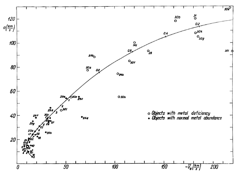
Figure 1: The relationship between the mean velocity dispersion $\sigma$ and the heliocentric rotation velocity $V_{\theta}$ for various subsystems of the Galaxy. Subsystems of different chemical composition are marked with different symbols, numbers are according to Tables 1, 2 and 3. The line shows the mean relationship of subsystems of various ages in billions of years, starting from the formation of the oldest populations.

3 The influence of selection and observational errors

In the study of the kinematical structure of main sequence star samples, we paid essential attention to the influence of selection and random errors (Einasto 1954, 1955a). Both effects were taken into account by Wehlau (1957). In other studies these factors were ignored, or discussed using methods which did not guarantee sufficient accuracy of results.

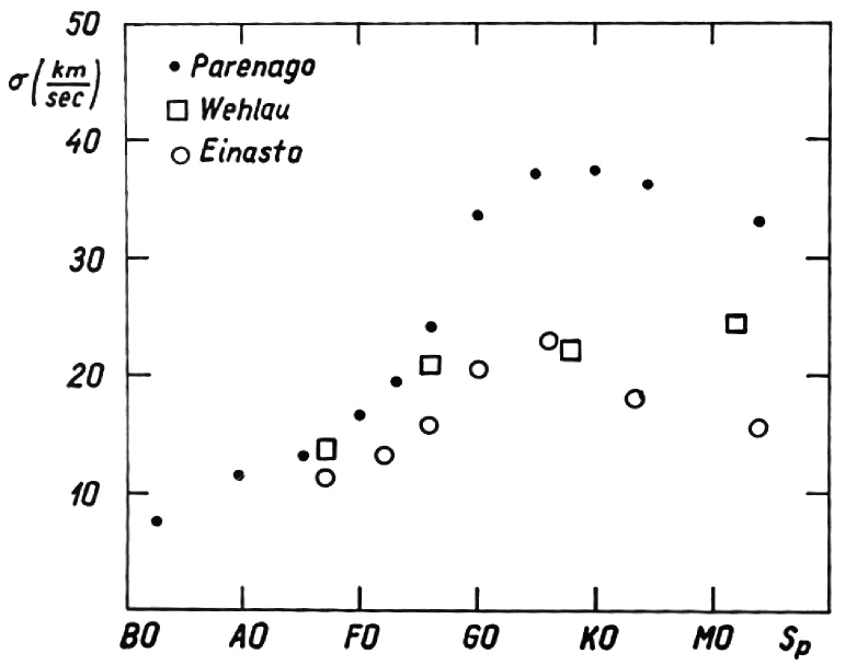
Figure 2: The mean velocity dispersion of main sequence stellar populations according to three authors. Due to ignoring observational errors, dispersions found by Parenago are considerably higher, and dispersions found by Wehlau slightly higher.

To illustrate the effect of these factors, we show in Fig. 2 kinematical characteristics of the stars of the main sequence according to Parenago (1951), Wehlau (1957) and Einasto (1954). We see that velocity dispersions $\sigma$ according to Parenago are much higher than dispersions obtained by other investigators. Data by Wehlau (1957) and Einasto (1954) are generally in good mutual agreement, there are only minor differences. We do not have original data by Wehlau (1957), thus we cannot estimate the cause of remaining differences. It is possible that the correction for observational errors by Wehlau was not correct. On the other hand, it is not excluded that we have overcorrected our samples for errors. For now, we accepted data from our determinations for main sequence stars.

Kinematical characteristics, corrected for selection and observational error effects, are printed in Tables 1, 2 and 3 in boldface.

The need to take into account these factors was known long ago, however, in most studies it was ignored. An exception is the work by Michałowska & Smak (1960), where the absence of stars with low velocities was taken into account. In similar studies by Yasuda (1961) and Eggen (1964), the selection effect was not taken into account, and we could not use these samples. Moreover, Eggen (1969a) divides stars into flat and disc populations using components of spatial velocities ($V_{R}$, $V_{\theta}$): stars within a defined region belong to the flat component, and stars outside this region to the disc component. This division ignores the presence of tails in velocity distribution of the flat component, and the presence of stars with low velocities in the disc component.

Also, we could not use the large catalogue of spatial velocity components by Eggen (1962), since the system of photometric parallaxes is voluntary, as shown by Weller et al. (1968).

4 Determination of population ages

One of the main goals of the present paper is the establishment of a relationship between kinematical characteristics and ages of populations.

The ages of samples of stars from the upper part of the main sequence were found either from the zero-age curve, shown in Fig. 1, or from the mean spectral type. The maximal age of main sequence stars can be found from Iben evolutionary tracks, see Chapter 22. Fast movement away from the main sequence starts at point Nr. 3 of Iben (1967c) track. We found that the respective age is related to the visual luminosity with a simple equation ($M_{V}\leq 5$):

$$\log\,t_{3}=8.19+0.353\,M_{V}.$$

This equation gives the maximal age of stars. Early stars of the main sequence have the mean age equal to half of the maximal age.

Stars of late spectral type of main sequence have large velocity dispersions and form a thick subsystem. For this reason, the spatial density of stars of this type is relatively small. Samples of stars are collected near the Solar vicinity, thus old stars are represented with a smaller frequency. For this reason, for F8 to G9 type stars of the main sequence we accepted mean ages slightly less than half of the maximal age. For stars of later spectral type, it is difficult to estimate this effect quantitatively, thus we did not try to find their mean age.

We attribute to sub-giants, white dwarfs and planetary nebulae an age equal to a half of the age of the whole Galaxy. These objects have large spread of ages, however, older stars dominate, which confirms our estimate.

The youngest Mira type variables with initial masses about $2.5\,M_{\odot}$ have ages slightly less than a billion years. However, the spread of periods of Miras of identical ages is large (Smak (1966b), Feast & Shuttleworth (1965)). For this reason, we accepted for Miras of the type 29g a larger age – 2 billion years.

To star samples with the largest velocity dispersion and centroid velocity (short period cepheids with $P\geq 0.6$ days), we attribute ages equal to the age of the whole Galaxy. As explained in Chapter 23, we accepted for the age of the Galaxy the round value 10 billion years.

Figure 1 shows that approximately at the point with coordinates $-\overline{V}_{\theta}=\sigma=50$ km/sec, a transition takes place from stars with metal deficit to stars of normal metal content. We attribute stars with metal deficit to the halo, and stars with normal metal content to the disc and the core. Calculations of the physical evolution of the Galaxy show (Sandage & Eggen (1969), Cameron & Truran (1971)) that the metal enrichment proceeds in the early phase of Galaxy evolution very rapidly, and that the mean chemical composition changes little later. For this reason, the second phase of the chemical evolution of the Galaxy has a long duration about 9 billion years, see Chapter 23. We conclude that at the point with $-\overline{V}_{\theta}=\sigma=50$ km/sec, the halo formation was finished, and the formation of disc started.

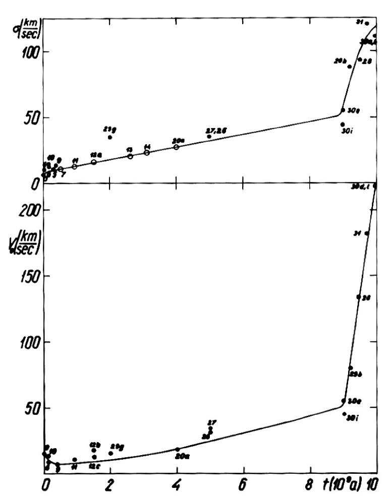
Figure 3: The dependence of the mean velocity dispersion $\sigma$ and heliocentric rotation velocity $V_{\theta}$ on the age $t$ of populations, according to Table 1. Open circles in the top panel show populations where it was possible to correct data for observational errors.

The problem of the duration of the formation of the halo, and the possibility that some halo and disc stars formed at the same time, is widely discussed. Eggen et al. (1962), and Sandage (1969, 1970) argued that the halo formed quickly during several hundred million years. On the other hand, Rood & Iben (1968) support a more extended period of halo formation, and that some halo stars formed after the start of disc star formation. Our data, shown in Fig. 1, suggest that some overlap in the formation of halo and disc stars is possible. Our calculations of the Galaxy evolution suggest that the formation of the halo could be slower than accepted by Eggen et al. (1962). However, the argument by Eggen et al. concerning the short formation scale of the halo must be correct.

Using these arguments, we accepted the ages of halo objects. Globular clusters have the largest axial ratios of equidensity ellipsoids (Chapter 20) and the smallest heavy element abundance. For globular clusters, we accepted ages longer than the mean age of the whole halo. To Mira variables with periods 150 – 200 days, we accepted an age $9.2\times 10^{9}$ yr. Miras of this type can be located in relatively rich globular clusters (Arp et al. (1963), Sandage et al. (1966), Rosino (1966)), which according to other data are younger than normal globular clusters.

We show in Fig. 3 the dependence of $\sigma$ and $\overline{V}_{\theta}$ on the age of subsystem $t_{S}$. For disc objects, we used data by Einasto (1954), where observational selection and error effects were studied in great detail. In the determination of the function $\overline{V}_{\theta}(t)$, we notice that selection and error effects shift values of $\sigma$ and $\overline{V}_{\theta}$ in a similar way, thus data points do not exit from the mean relationship curve. We can consider the Fig 3 as a parametric presentation of the mean relationship in Fig. 1.

Table 4: Kinematical data on Galaxy populations

ID	$k_{\theta}$	$-\Delta\,e$	$-\Delta\,h$	$(k_{\theta})_{0}$	$k_{z}$	$-\Delta\,e$	$(k_{z})_{0}$
10	0.44	0.01	0.00	0.43	0.25	0.005	0.245
12	0.44	0.01	0.00	0.43	0.32	0.005	0.315
16	0.34	0.01	0.01	0.32	0.26	0.005	0.255
17	0.46	0.01	0.03	0.42	0.31	0.005	0.305
18	0.37	0.01	0.00	0.36	0.18	0.005	0.175
21	0.46	0.01	0.00	0.45	0.29	0.005	0.285
22	0.55	0.01	0.10	0.44	0.30	0.005	0.295
23	0.55	0.01	0.10	0.44	0.44	0.005	0.435
26	0.41	0.01	0.02	0.38	0.31	0.005	0.305
27	0.50	0.01	0.06	0.43	0.21	0.005	0.205

5 Ratios of semiaxes of velocity ellipsoids

Ratios of semiaxes of velocity ellipsoids are important parameters, characterising the local structure of the Galaxy. Our collection of kinematical data allows to get new estimates of these parameters.

As we see later in Chapter 21, very young stellar populations are not in a stationary state. On the other hand, very old populations have ratios of velocity ellipsoid semiaxes, different from ratios found for young flat populations. For this reason, we shall use in the determination of mean values of ratios $k_{\theta}$ and $k_{z}$ only subsystems in the velocity dispersion interval from 15 to 50 km/sec. Mean values of $k_{\theta}$ and $k_{z}$ in this $\sigma$ interval, collected from data given in Table 1 - 3, are given in Table 4.

To find mean values of $k_{\theta}$ and $k_{z}$, the influence of observational errors must be taken into account. This error makes the velocity ellipsoid rounder. Furthermore, it is needed to take into account the kinematical heterogeneity of observation data. The asymmetric shift of the velocity ellipsoid increases the dispersion ratio $k_{\theta}$. A theory of this factor was developed by Eelsalu (1958). We estimated corrections $\Delta\,e$ and $\Delta\,h$ using data on the inhomogeneity of star samples, and mean errors of stellar parallaxes. Results are given in Table 4 as well as the corrected values of $(k_{\theta})_{0}$ and $(k_{z})_{0}$. The overall mean values and their estimated errors are: $(k_{\theta})_{0}=0.410\pm 0.015$ and $(k_{z})_{0}=0.278\pm 0.010$.

6 Circular velocity in the Solar vicinity

Our collection of data allows to calculate the circular velocity near the Sun, using the theoretical Strömberg asymmetry equation (Einasto & Kutuzov 1964b)

$$V_{i}^{2}-(G_{i}+m_{0})\,\sigma_{Ri}^{2}=V^{2},$$ (3)

where $V_{i}$ is the galactocentric rotation velocity of subpopulation $i$, $\sigma_{Ri}$ is the velocity dispersion in radial direction of this subsystem, $V$ is the circular velocity,

$$G_{i}=G\{\rho(R)\}_{i}=\frac{\partial\ln\rho_{i}}{\partial\ln\,R}$$ (4)

is the logarithmic gradient of the density, and

$$m_{0}=(1-k_{\theta})+n_{R}(1-k_{z})$$ (5)

is a quantity, equal for all Galaxy subsystems. Here we used designations identical to Eq. (19).

Galactocentric centroid velocity $V_{i}$ can be expressed through the $\theta$-component of the heliocentric centroid velocity $\overline{V}_{\odot}$ using the equation

$$V_{i}=V+(\overline{V}_{\odot}-V_{\odot}),$$ (6)

where $V_{\odot}$ is the $\theta$ component of the Solar velocity in respect to the circular velocity.

Using our collected data as well as data by Blaauw & Schmidt (1965) on the density gradient, we found for flat populations

$$V_{\odot}=-9.0\pm 0.2\leavevmode\nobreak\ {\rm km/sec},$$ (7)

which yields, using data of intermediate and spherical populations,

$$V=226\pm 21\leavevmode\nobreak\ {\rm km/sec}.$$ (8)

Error of this determination of the circular velocity is fairly large, it is determined by errors in the density gradient and velocity dispersion.

We note that this method to determine the circular velocity in the Solar neighbourhood was applied earlier by Parenago (1951).

September 1971

Chapter 6 Model of the Galaxy and the system of Galactic parameters: Preliminary version

This Chapter presents our first attempt to bring together the available data on the structure of the Galaxy in a model, and to find the system of Galactic parameters. The model was presented in the talk by Einasto (1965) in the conference “Kinematics and dynamics of stellar systems and physics of the interstellar medium” in Alma-Ata in summer 1963.

1 Introduction

In order to bring together the available data on the structure of stellar systems and to determine their gravitational field, appropriate models are used. Naturally, particular attention is paid to the building of the model of our Galaxy. Work in this direction has been going on in Tartu for more than ten years. At first we were interested mainly only in the radial distribution of masses in the Galaxy (Kuzmin 1952a, 1956b). As for the spatial distribution, the models were not specified, or special models were used by Kuzmin (1956a); Kuzmin & Kutuzov (1962). At the present time we set the task of building a more detailed model of the Galaxy without trying to base it on any special assumptions.

The problem of constructing a model of the Galaxy is closely related to the problem of constructing a system of Galactic parameters, and the application of the equations of stellar systems hydrodynamics. The hydrodynamics of stellar systems is considered in the paper by Kuzmin (1965), and the problem of determining the Galactic parameters is discussed in the paper by Kutuzov (1965). The present paper considers the problem of constructing a model of the Galaxy and determining the system of Galactic parameters from a practical point of view, and provides some preliminary results of calculations.

The main task in the construction of the Galactic model is the determination of the mass distribution function in it. In the first rough approximation we can assume that surfaces of equal densities in the Galaxy are similar ellipsoids of rotation, having a common axis and a symmetry plane. In such an assumption, the radial mass distribution is found from the circular velocity by a solution of the integral equation:

$$V^{2}(x)=G\,\int_{0}^{x}{\mu(a)\,{\rm d}a\,\over\sqrt{x^{2}-e^{2}a^{2}}},$$ (1)

where $V$ is the circular velocity in the symmetry plane of the system; $G$ is the gravitational constant; $x$ is the distance from the symmetry axis; $a$ is the semi-major axis of an ellipsoid of equal density; $e=\sqrt{1-\epsilon^{2}}$, with $\epsilon$ being the ratio of the ellipsoid minor to major axes and, finally, $\mu(a)\,{\rm d}a\,$ is the mass contained between ellipsoids with semi-major axes $a$ and $a+{\rm d}a\,$. It is reasonable to express the values of $a$ and $x$ in units of the Sun’s distance from the center of the system $R_{0}$. In this case, for the mass function $\mu(a)$ we have the expression:

$$\mu(a)=4\pi\,R_{0}^{2}\,\epsilon\,\rho_{0}\,a^{2}\,\rho^{\star}(a).$$ (2)

where $\rho^{\star}(a)$ is the volume mass density on the surface of an ellipsoid with semi-major axis $a$ in units of the circumsolar density $\rho_{0}$.

Several variants of equation (1) and methods of its solution have been proposed by different authors. For example, Wyse & Mayall (1942) and Schwarzschild (1954) consider a flat model of the stellar system. In this case $\epsilon\rightarrow 0$ and $\rho\rightarrow\infty$, but $\mu$ remains finite. Instead of $\mu$ they use the surface density $P$, making an integral equation for it. The surface density is related to the mass function by a simple integral relation (see Kuzmin (1956b)).

Kuzmin (1952a, 1956b), Perek (1951, 1954) and Takase (1955) already represented the Galaxy as an inhomogeneous ellipsoid. In this case we have a spatial model of the system. However, the surfaces of equal density are not in fact similar ellipsoids. To eliminate this drawback, Kuzmin (1956b) proposed a generalised spheroidal model consisting of a large number of individual spheroids. The presence of spheroids was taken into account by introducing some mean values of $\epsilon$ and $e^{2}$ as functions of $a$.

In Kuzmin’s generalised model we already have three unknown functions — $\rho(a)$, $\epsilon(a)$, and $e^{2}(a)$. It is clear that it is impossible to solve one integral equation with three unknown functions. If we attract additional observational material on the density distribution, and the ratio of semi-major axes of individual subsystems, and are interested not only in determining the mass or surface density function but also the spatial density of the Galaxy, it is more natural and simple to consider subsystems in explicit form, without resorting to the average $\epsilon$ and $e^{2}$. This is the path followed by most of the authors who have recently studied the mass distribution in the Galaxy (Schmidt (1956), Perek (1954), Idlis (1961a)).

With respect to individual subsystems of the Galaxy, if they are physically homogeneous groups of stars, we can assume with a much better approximation than for the Galaxy as a whole that surfaces of equal density are similar ellipsoids of rotation. The mass function $\mu(a)$ and the ratio of ellipsoid semiaxes $\epsilon_{i}$ are, of course, different for different subsystems. Summing up the contributions of individual subsystems to $V^{2}$, we obtain:

$$V^{2}(x)=4\pi\,G\,R_{0}^{2}\,\sum_{i}\,\epsilon_{i}{\rho_{0}}_{i}\,\int_{0}^{x}{a^{2}\rho_{i}^{\star}(a){\rm d}a\,\over\sqrt{x^{2}-e_{i}^{2}a^{2}}}.$$ (3)

In equation (3), both the circular velocity functions $V$ and the subsystem density distribution functions $\rho_{i}^{\star}$ are known with some accuracy. The parameters of this formula, $R_{0}$, $\epsilon_{i}$ and ${\rho_{0}}_{i}$, are also known approximately. Therefore, the expression (3) should be considered not as an integral equation for determining the mass distribution in the Galaxy but as an equation for mutual agreement and specification of the functions and parameters appearing in it.

2 Observational data

The following observational data are available to build a model of the Galaxy:

(a) for the nearest neighbourhood of the Sun, there are kinematical data with respect to all subsystems of the Galaxy, and data on the spatial distribution of most subsystems (excluding subsystems of absolutely faint stars);

(b) for wide regions of the Galaxy, comparable to the size of the whole stellar system, the spatial distribution is known only for a few subsystems, among which, fortunately, representatives of all main components of the Galaxy appear; in addition, the rotation of some flat component subsystems is known;

(c) data on rotation and surface density distribution of other galaxies, which to some extent supplement the information about our Galaxy, especially for central and peripheral regions.

As we can see, the observational data are very limited, so the full description of the Galaxy in the six-dimensional phase space is out of the question. However, they are sufficient to determine the overall trends of the mass density distribution for the main components of the Galaxy. It is possible to determine a number of other functions characterising the structure of the Galaxy.

As a function approximating the density distribution of Galactic components, we have chosen a generalised exponential law

$$\rho^{\star}(a)=e^{-{m_{0}\over\nu}\,(a^{\nu}-1)},$$ (4)

where $\nu$ is some positive number, characterising the degree of mass concentration to the center of the system, and $m_{0}$ is the density logarithm gradient near the Sun:

$$m=-{\partial\,\ln\,\rho(a)\over\partial a}=-{R\over Mod}{\partial\log\rho(R)\over\partial R}.$$ (5)

In particular cases $\nu=2$ and $\nu=1$, we have Gaussian and ordinary exponential distributions, which have already been repeatedly applied to describe the spatial density of galaxy subsystems (Perek (1951), Takase (1955), Perek (1958)). On the other hand, de Vaucouleurs (1948, 1953) showed that surface brightness of elliptical galaxies and spherical components (core and halo) of spiral galaxies can be represented using function (4) with $\nu=0.25$. If we assume that the mass-to-light ratio for the spherical component of a given galaxy does not change with the distance from the system’s centre, the surface brightness is proportional to the surface mass density. By solving the corresponding integral equation, we found the spatial density distribution. It turned out that the same function, (4) is obtained with sufficient accuracy but with $\nu=0.18$. Thus, the spherical components of galaxies can be described by the formula (4) with a small value of $\nu$.

The generalised exponential distribution (4) is convenient, because it is defined in an infinite interval, and therefore takes into account the presence in the stellar system of stars with very elongated orbits, whose velocities are close to the parabolic. On the other hand, the density decreases quickly enough at large distances, so that the mass of the model is finite, and the model does not have such an extensive envelope as the Kuzmin model, derived from the third integral theory (Kuzmin 1956a). Furthermore, the distribution at different $\nu$ gives a very different course of the density logarithm gradient, decreasing ($\nu<1$) or increasing ($\nu>1$) with increasing $a$.

It is sufficient to represent the Galaxy as a composite model for three components: planar (Flat), intermediate (Disc), and spherical (Sph). The parameters characterising the structure of the components are given in Table 1. The values obtained on the basis of observational material are given in the column 0, and the values obtained by equating the observed values are given in the column 1.

Table 1: Parameters of Galaxy populations

Pop.	$i$	$\nu_{i}$	$\overline{|z|_{i}}$	$\epsilon_{i0}$	$\epsilon_{i1}$	$m_{i0}$	$m_{i1}$	$\rho_{0i0}$	$\rho_{0i1}$	$\frac{M_{i}}{M}$	Ref.
Flat	1	2	145	0.022	0.022	2.35	2.35	$30\pm 5$	25.0	0.041	17 - 20
Disc	2	1	400	0.09	0.13	4.00	3.30	$55\pm 10$	53.3	0.692	17, 21, 22
Sph.	3	1/3	2300	0.60	0.60	3.10	3.91	$2\pm 2$	1.89	0.267

Notes: $\overline{|z|_{i}}$ is given in parsecs; densities $\rho_{0i0}$ in $M_{\odot}$ per kiloparsec³.
References are: 17 – Oort (1958), 18 – Westerhout (1957), 19 – Schmidt (1957a), 20 – Kopylov & Kumaigorodkaya (1955), 21 – Kopylov (1955), 22 – Kukarkin (1949); references for spherical components are: Kukarkin (1949), de Vaucouleurs (1953), Perek (1954), Schmidt (1956), Schmidt (1957a), Notni (1956), Oort (1958), Baade (1958), Oort (1960a), Johnson & Svolopoulos (1961), Wallerstein (1962), Lozinskaya & Kardashev (1963).

To calculate the flattenings of the components, we determined the flattenings of the various subsystems of the Galaxy, using the formula

$$\epsilon={\sqrt{m}\zeta\over sR_{0}},$$ (6)

where $\zeta$ is a parameter characterising the distribution of stars in the direction perpendicular to the Galactic plane, and $s$ is a dimensionless coefficient of the order of unity. The formula (6) is derived under the assumption that within subsystems the surfaces of equal density are similar ellipsoids. The parameter $\zeta$ can take, for example, one of the following values:

$$\begin{array}[]{ll}\zeta_{l}={R_{0}\over l}=\left(-{\partial^{2}\,\ln\rho(z)\over\partial z^{2}}\right)_{z=0}^{-1/2},&\zeta_{0}=z_{0}={1\over\rho(0)}\int_{0}^{\infty}{\rho(z){\rm d}z\,},\\ \\ \zeta_{1}=\overline{|z|}={\int_{0}^{\infty}{z\rho(z){\rm d}z\,}\over\int_{0}^{\infty}{\rho(z){\rm d}z\,}},&\zeta_{2}^{2}={\int_{0}^{\infty}{z^{2}\rho(z){\rm d}z\,}\over\int_{0}^{\infty}{\rho(z){\rm d}z\,}}.\end{array}$$ (7)

Here $l$ is the parameter introduced by Kutuzov (1965), $z_{0}$ is the equivalent half-thickness of the Galaxy (Kuzmin 1952a). The numerical value of the coefficient $\zeta$ depends on the particular kind of density distribution. If we accept the law (4) for the density, then for $\nu=2$ and $\nu=1$ we have the values given in Table 2. It should be said that $\zeta_{0}=1$, regardless of the particular kind of density distribution.

Table 2:

Comparing our derived values $\epsilon$ with the results of Schmidt (1956) and Idlis (1961b), we can say the following. The ratio of semiaxes for the planar component agrees well with the results of other authors. Only for the central regions of the Galaxy Idlis took $\epsilon=0.25$ in order to have a smaller spatial density for a given surface density. It is difficult to agree with this, however, as direct estimates (Westerhout (1957), Lozinskaya & Kardashev (1963)) indicate that the thickness of the interstellar hydrogen layer, the main subsystem of the flat component of the Galaxy, does not increase as we approach the centre of the system, but, on the contrary, decreases. The data on the ratio of half-axes for the intermediate component agree with Schmidt’s data (Idlis does not consider this component in his model). The data for the spherical component differ strongly. Schmidt took $\epsilon=0.16$ in this case, which is clearly insufficient. Idlis took for the peripheral regions of the Galaxy an average of $\epsilon=0.5$, which is quite acceptable. However, in the centre of the system he took an underestimated value of $\epsilon=0.25$. Photographs of spiral galaxies, visible from the edge, show that the nuclei of these systems have an $\epsilon$ of the order of $0.5-0.7$ (Johnson (1961), de Vaucouleurs (1959)). The apparent decrease of $\epsilon$ for the inner regions in the subsystems of globular clusters and short-period cepheids, noted by Idlis, is caused by the fact that these subsystems are not homogeneous but consist of a mixture of objects of intermediate and spherical components (Notni (1956), Baade (1958)).

The $\nu$ parameter was chosen so that the law (4) satisfactorily represented the available data on the density distribution of the planar (Westerhout (1957), Schmidt (1957a)), intermediate (Kukarkin (1949), de Vaucouleurs (1959)), and spherical (Kukarkin (1949), de Vaucouleurs (1948, 1953), de Vaucouleurs (1959), Oort (1960a)) subsystems.

The gradient $m$ for the intermediate component was taken from Idlis (1961b) summary, while for the planar and spherical ones it was calculated anew. It turned out that the earlier determinations of this gradient for the spherical subsystems were exaggerated.

In addition to data on the structure of the individual components, in order to derive a system of Galactic parameters and build a model of the Galaxy, we also need knowledge of the course of the circular velocity. The observational material needed for this purpose is available in the form of radio astronomical determinations of the differential rotation of interstellar hydrogen. We used the data of Dutch scientists in the treatment by Kwee et al. (1954) and Agekyan & Klosovskaya (1962). Based on this material, we compiled for eight values of $x$ the normal points of the Galactic differential rotation function $U$. This function is related to the circular velocity $V$ by the formula

$$V(x)=U(x)+x\,V_{0},$$ (8)

where $V_{0}$ is the circular velocity in the vicinity of the Sun. The results, together with estimates of their average errors, are given in Table 3. The values obtained on the basis of observational material are given in the column 0, and the values obtained by smoothing the observed values are given in the column 1.

Table 3: Differential rotation function $U(x)$ of the Galaxy

Finally, we used a number of other parameters, the circumsolar values of which, together with their errors, are given in Table 4.

Table 4: Near-solar values of galactic parameters

References: (30) Kwee et al. (1954), (31) Agekyan & Klosovskaya (1962), (32) Baade (1951), (33) Whitford (1961), (34) Weaver (1954), (35) Feast & Thackeray (1958), (36) Parenago (1951), (37) Fricke (1949a), (38) Fricke (1949b), (40) Stibbs (1956), (41) Petrie et al. (1956), (42) Gascoigne & Eggen (1957), (43) Walraven et al. (1958), (44) Janák (1958), (45) Pskovskii (1959), (46) van de Kamp & Vyssotsky (1937), (47) Raymond & Wilson (1938), (48) Vyssotsky & Williams (1948), (49) Morgan & Oort (1951), (50) Oort (1932), (51) Kuzmin (1952b), (52) Kuzmin (1955), (53) Eelsalu (1961), (54) Dyer (1956).

In deriving the distance to the centre of the Galaxy, only independent estimates were taken into account, the dynamical determinations were not used. The latter depend on other Galactic parameters; in the subsequent least-squares processing, however, it was assumed that all the estimates of the parameters to be equated must be independent.

The circular velocity is determined mainly dynamically by the asymmetric shift of the velocity centroids of the stars (Parenago 1951). These data as well as the corresponding formula do not appear anywhere else in the construction of the system of Galactic parameters, so that the velocity definition can be considered independent. In addition, general dynamical considerations (Fricke 1949a, b) were taken into account, according to which $V_{0}$ cannot be much less than 275 km/s.

The kinematical parameter, $W=-1/2\,({\rm d}U\,/{\rm d}x\,)_{x=1}$, characterises the circumsolar value of the Galactic differential rotation function, based on the behaviour of the $U$ function (see Table 3). This value is somewhat smaller than that usually accepted (Schmidt (1956), Lozinskaya & Kardashev (1963)) and nearly coincides with the value obtained by Idlis (1961b) (see Table 4).

We consider the Oort-Kuzmin parameters $A,B$, and $C$ in the dynamical sense, i.e. corresponding to the gravitational acceleration along $R$ and $z$.

When calculating the Oort parameter $A$, only values giving $A>15$ km/sec/kpc were taken into account. The significantly lower values obtained by some authors are distorted, apparently, by local features of some subsystems of stars, or by drawbacks in the methodology of material processing. In calculating the average error of $A$, we took into account the fact that many authors used practically the same observational material.

The parameter $B$ is known to be different in the GC and FK3 system. Most astronomers prefer the FK3 system, in which $B=-7$ is obtained. This value leads, however, to various dynamical difficulties (Kuzmin 1956b). Therefore, we took the average of the $B$ values in the GC and FK3 systems, increasing the mean error, which, in addition to the random error, also takes into account the unknown systematic error.

The parameter $C$ is taken from the determinations by Kuzmin (1952b) and Eelsalu (1958), for definition see Chapter 6. The markedly larger values, obtained by some authors, are distorted, as pointed out by Eelsalu (1958, 1961), by the imperfection of the applied methodology.

The ratios of velocity dispersions of stars:

$$k_{\theta}={\sigma_{\theta}^{2}\over\sigma_{R}^{2}},\hskip 28.45274ptk_{z}={\sigma_{z}^{2}\over\sigma_{R}^{2}},$$ (9)

were taken from Parenago (1951) and Dyer (1956). In these works, the components of the spatial velocities of stars are used, and the material is divided by physical features into separate subsystems. The definitions of the dispersion relations, obtained from the proper motions (Hins & Blaauw 1948), were not taken into account. Apparently, they are distorted by systematic errors, which was pointed out by Trumpler & Weaver (1953).

3 Construction of the Galactic model and determination of Galactic parameters

When building a model of the Galaxy, it is assumed that there are a number of theoretical relations linking the parameters determined from observations. Equations (1) or (3) and the Poisson’s formula are usually used as such relations. We use the Poisson equation in the form, suggested by Kuzmin (1952b)

$$4\pi\,G\rho_{t}=C^{2}-2\,(A^{2}-B^{2}),$$ (10)

where $\rho_{t}$ is the total spatial density of mass. Also we use the Lindblad equation:

$$k_{\theta}={-B\over A-B},$$ (11)

and the following expressions derived from the definition of $A$, $B$, and $W$:

$$A\,R_{0}-W=0,$$ (12)

$$R_{0}(A-B)-V_{0}=0.$$ (13)

To these we can add another differential consequence of Eqn. (3)

$${{\rm d}V^{2}\,(x)\over{\rm d}x\,}=4\pi\,GR_{0}^{2}\,\sum_{i}\epsilon_{i}{\rho_{0}}_{i}{{\rm d}\int_{0}^{x}{{a^{2}\rho_{i}^{2}(a){\rm d}a\,\over\sqrt{x^{2}-e_{i}^{2}a^{2}}}}\,\over{\rm d}x\,}$$ (14)

and Kuzmin (1961) equation:

$$k_{z}^{-1}=1+k_{\theta}^{-1}.$$ (15)

Due to random and unaccounted for systematic errors in the definition of parameters or description functions as well as the inaccuracy of the applied theory, these equations are not fulfilled quite accurately. In order for the equations to be satisfied, one has to change the parameters and description functions somewhat. So far this has been done by trial-and-error procedure, and the result has depended heavily on the taste of the author. Moreover, a certain system of rounded values of the main parameters was often taken (for example, by Schmidt (1956) for $A$, $B$, $C$, $W$), while all other parameters were not taken from observations but were calculated by formulas (10) - (13).

An objective way to derive the best system of Galactic parameters and to construct the corresponding model of the Galaxy is the application of the least-squares method. In this case equations (3) and (10) - (15) are considered not as expressions for determination of this or that quantity but as fundamental equations to the equalisation of the system of Galactic parameters (Kutuzov 1965).

We performed the parameter equalisation twice, with and without the use of the model of mass distribution in the Galaxy. Such a way of solving the problem was chosen in order to find out the suitability of the model (4) to describe the structure of the Galactic components.

In the first case, the following quantities were equated by the least-squares method: the circumsolar densities of the intermediate and spherical components $\rho_{02}$ and $\rho_{03}$; the circumsolar value of the circular velocity $V_{0}$, kinematical parameter $W$; the Kuzmin parameter $C$; values of the function $U$ for eight points (see Table 3). Equations (3), (10), and (14) were used as fundamental equations, and expression (8) was substituted for $V(x)$ in (3) and (14), and expression (4) was substituted for $\rho_{i}^{\ast}(a)$. Calculation results are given in Tables 1, 3, and 4 (option 1).

In the second case, the circumsolar values of the following quantities were fixed: the Oort parameters $A$, $B$, the circular velocity $V_{0}$, parameter $W$, the distance from the centre of the Galaxy $R_{0}$, and the ratios of velocity dispersions, $k_{\theta}$ and $k_{z}$. As fundamental equations we used formulas (11) - (13) and (15). The results are given in Table 4 (option II).

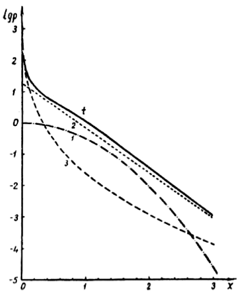
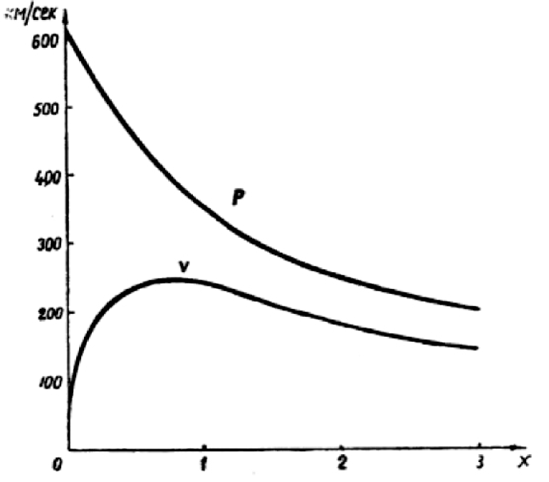
Figure 1: Left: Distribution of the logarithm of the density in units of the circumsolar total density, $\rho$ is the total density; 1, 2, and 3 are the densities of the planar, intermediate, and spherical components. Right: Dependence of the circular and parabolic velocity on the distance to the centre of the Galaxy.

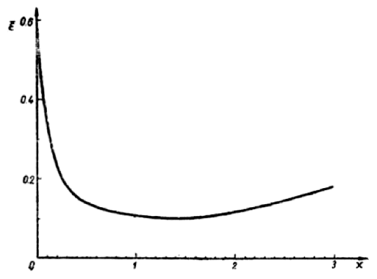
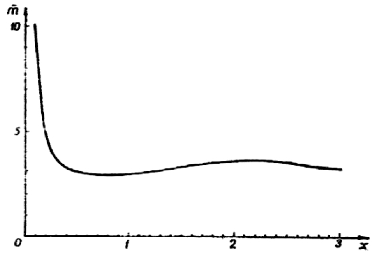
Figure 2: Left: The dependence of the average ratio of the semi-axes on the distance to the centre of the Galaxy. Right: Dependence of the average gradient of the logarithm of the density $m$ on the distance to the centre of the Galaxy.

In addition, we calculated the mean values of the ratio of the semi-axes $\overline{\epsilon}$ and the gradient $\overline{m}$ (with the weight $\rho_{t}$), the total mass of the Galaxy,

$$M=4\pi\,R_{0}^{3}\sum_{i}\epsilon_{i}{\rho_{0}}_{i}\,M_{2j}^{\star},$$ (16)

and the parabolic velocity $P=\sqrt{2\Phi}$ (where $\Phi$ is the gravitational potential):

$$P^{2}(x)=2\int_{x}^{\infty}{V^{2}(x){\rm d}x\,\over x}=8\pi\,G\leavevmode\nobreak\ R_{0}^{2}\sum_{i}\epsilon_{i}{\rho_{0}}_{i}\,\Phi_{i}^{\star}(x).$$ (17)

In formula (17) $\Phi_{i}^{\star}(x)$ is the mass of the subsystem in units $4\pi\,R_{0}^{3}\epsilon{\rho_{0}}_{i}$. The coefficient $M_{2j}^{\star}$ is a special case, $j=2$, of the moments of $M_{ji}^{\star}$ of the function $\rho_{j}^{\star}(a)$. If we take expression (4) for $\rho_{j}^{\star}(a)$, in the general case we have:

$$M_{ji}^{\star}=\int_{0}^{\infty}{a^{j}\rho_{i}^{\star}(a){\rm d}a\,}={1\over\nu}\exp\left({m_{0}\over\nu}\right)\,\left({m_{0}\over\nu}\right)^{-{1+j\over\nu}}\,\Gamma\left({1+j\over\nu}\right),$$ (18)

where $\Gamma$ is gamma-function.

The functions $\Phi_{i}^{\star}(x)$ in formula (17) are gravitational potentials of subsystems in plane $z=0$ in units $4\pi\,GR_{0}^{2}\epsilon_{i}\rho_{0i}$. They are calculated by the formula

$$\Phi_{i}^{\star}(x)=\int_{0}^{\infty}{\rho_{i}^{\star}(a)\chi_{i}\left({a\over x}\right)\,a{\rm d}a\,},$$ (19)

where

$$\chi_{i}\left(\frac{a}{x}\right)=\left\{\begin{array}[]{ll}\frac{1}{e_{i}}\arcsin(\frac{e_{j}a}{a}),&a\leq x,\\ \frac{1}{e_{i}}\arcsin(e_{i}),&a\geq x.\end{array}\right.$$ (20)

For $x=0$ (Galactic center) we have as a special case

$$\Phi_{i}^{\star}(0)={\arcsin(e_{i})\over e_{i}}\,M_{1i}^{\star},$$ (21)

and for large $x$ we obtain the following asymptotic decomposition:

$$\Phi^{\star}(x)\approx\frac{M_{2}^{\star}}{a}\left[1+\frac{1}{2}\frac{1}{3}\left(\frac{e}{x}\right)^{2}\frac{M_{4}^{\star}}{M_{2}^{\star}}+\frac{1}{2}\frac{3}{4}\frac{1}{5}\left(\frac{e}{x}\right)^{4}\frac{M_{6}^{\star}}{M_{2}^{\star}}+\dots\right].$$ (22)

4 Conclusions

The equalisation in the first variant with the original initial data (column 0 in Tables 1, 3, and 4) did not yield satisfactory results. The obtained system of Galactic parameters differed markedly from that in the second variant, the calculated circular velocity curve had an unacceptable discrepancy with the observed curve. However, it turned out that the obtained circular velocity curve was very sensitive to changes in the parameters of formulas (3) and (4) for the intermediate and spherical components. The planar component makes such a small contribution to the expression for $V^{2}$ (less than 5%) that the $V^{2}$ curve almost does not depend on its parameters. After slightly changing $\epsilon$ and $m$ (Table 1, variant I) of the intermediate and spherical component, we carried out the equation anew; the results were satisfactory this time. Their agreement both with the original data and with the results of equalisation without the model (variant II) is good. Errors of parameters after adjustment in variant II turned out to be notably smaller.

The logarithms of densities of components and total densities, the mean values of the ratio of half axes and the gradient of the density logarithm, and the circular velocity are given in Figures 1 and 2. In the calculations, we took the Galactic parameters according to variant I. The values of density $\rho_{3}$ and $\rho_{t}$ at $x=0$ correspond to average density in ellipsoid with semi-major axis $a=0.0016$, gradient $m$ is calculated for distance $x=0.001$ (at $\nu<1$ $m\rightarrow\infty$ if $x\rightarrow 0$).

Let us now compare the obtained preliminary systems of Galactic parameters with those derived from the models by Kuzmin (1955), Schmidt (1956) and Idlis (1961b) (see Table 4).

Kuzmin’s system differs from the others in the "classical" values of the parameters $A_{0}$, $B_{0}$ and $R_{0}$. The mean $\epsilon$ of the model is somewhat exaggerated, since the values of $A_{0}$ and $B_{0}$ were taken too large, and, besides, a very rough model of the Galaxy was taken when calculating $\epsilon$ (formula (56) in Kuzmin (1952b)).

Schmidt’s system is markedly different from ours. It assumes $B$ in the FK3 system, which leads to underestimated values of the circular and parabolic velocity as well as the ratio $k_{\theta}$ but, on the other hand, to an unacceptably high value of the gradient $m_{0}$. Recently, Schmidt (1961, 1962) has become convinced of the necessity to reduce the density gradient.

Schmidt’s model has too small dimensions and sharp boundaries due to large density gradient. This leads to an excessively fast decrease of the circular velocity with increasing distance, and a small value of the escape velocity.

Our system of parameters agrees well with Idlis’s system. But Idlis’s model has a significant drawback — by adopting Parenago’s law for the circular velocity, Idlis was not able to take into account the presence in the Galaxy of a very dense and quite massive nucleus and an extensive halo.

October 1963

Chapter 7 System of Galactic parameters

In this Chapter, we present a method of the determination of the system of Galactic parameters, using equations, connecting parameters as fundamental equations to the equalisation of the system of Galactic parameter, using observational estimates of all parameters. The idea of the method was described by Kutuzov (1964). The new system was presented by Einasto & Kutuzov (1964a, b) to the Commission 33 Meeting, IAU XII General Assembly, Hamburg, 1964.

In the following years, I continued to collect observational data on all Galactic parameters which enter in the system of parameters. Results of this search were collected in Chapter 6 of the original Thesis on 56 pages of typed text with 14 tables and a reference list with 159 entries. However, these data were not used to construct a new model, because in 1971 I was busy calculating the physical evolution of galaxies, and there was no time to find a new model of the Galaxy. Soon it was evident that the model should include a massive, extensive and almost spherical component — corona. This changes the gravitational potential field of the Galaxy, which influences Galactic parameters, thus the collected data on parameters became obsolete. For this reason, this collection is not reproduced in the current English version of the Thesis. I present here only the main idea of the method to determine the system of Galactic parameters, and the 1964 version of parameters. The preliminary 1963 version of the Galactic model with parameters was published by Einasto (1965) and is presented in Chapter 5, the 1970 version of Galactic parameters was described by Einasto (1970a) and is presented in Chapter 7. A preliminary model of the Galaxy with massive corona and respective system of parameters was presented by Einasto (1979) and is described in the Epilogue. Our final model of the Galaxy with an improved system of Galactic parameters was published by Haud & Einasto (1989).

As Galactic parameters, the following parameters or constants are usually considered:

$R_{0}$ — the distance of the Sun from the Galactic centre,

$A$, $B$ — Oort’s rotational parameters, referring to the circular motion,

$\rho_{0}$ — the Galactic mass density in the solar neighbourhood.

Given the first three of these parameters, the circular velocity

$$V=R_{0}(A-B)$$ (1)

can be found.

To obtain the numerical values of these parameters, their direct estimates can be used. On the other hand, the estimates of the following quantities can be applied for this purpose: the Kuzmin parameter

$$C=\frac{\sigma_{z}}{\zeta},$$ (2)

the gradient of the function of differential rotation velocity

$$W=-\frac{1}{2}\,\left(\frac{{\rm d}U\,}{{\rm d}\xi\,}\right)_{\xi=1},$$ (3)

and the ratio of velocity dispersions

$$k_{\theta}={\sigma_{\theta}^{2}\over\sigma_{z}^{2}}.$$ (4)

In these formulae $\sigma_{R}^{2}$, $\sigma_{\theta}^{2}$ and $\sigma_{z}^{2}$, are the velocity dispersions in Galactic cylindrical coordinate system, $\zeta$ is the $z$-coordinate dispersion, $U$ is the function of differential Galactic rotation, obtained from radio observations (Kuzmin 1956a), and $\xi=R/R_{0}$. Three parameters, $C,\leavevmode\nobreak\ W$ and $k_{\theta}$, are connected with the former ones by equations (see Chapters 5 and 7):

$$4\pi\,G\,\rho_{0}=C^{2}-2\,(A^{2}-B^{2}),$$ (5)

$$W=A\,R_{0},$$ (6)

$$k_{\theta}=\frac{-B}{A-B}.$$ (7)

In the old system of Galactic parameters (Schmidt 1956), the parameters $A$ and $B$ were taken from proper motion studies ($A=19.5$ and $B=-6.9$ km/sec/kpc), and $R_{0}$ was calculated by means of formula (6) from $W=160$ km/sec, which yielded $R_{0}=8.2$ kpc, in good agreement with directly obtained value. For the circular velocity the value $V=216$ km/sec was obtained.

In the new system of Galactic parameters, accepted at the Australia symposium on Galactic structure (Oort 1965), the following rounded values were proposed:

$R_{0}=10$ kpc,

$V=250$ km/sec,

$A=15$ km/sec/kpc,

$B=-10$ km/sec/kpc,

$\rho_{0}=0.145\leavevmode\nobreak\ M_{\odot}$/pc³.

This yields:

$C=90$ km/sec/kpc,

$W=150$ km/sec,

$k_{\theta}=0.40$.

It should he emphasised, however, that it is possible to widen the amount of observational data used, introducing new equations and new parameters, for which observed estimates are present. Furthermore, by applying the least-squares method, it is possible to improve the procedure of obtaining the system of parameters,

Besides the parameters characterising the Galactic structure in general, the population parameters may be used. Practically it is possible to use the heliocentric centroid velocities $V_{i}$, the dispersions $\sigma_{Ri}^{2}$, and the radial logarithmic density gradients $m_{i}=-R_{0}\,{\rm d}\ln\,\rho_{i}\,/{\rm d}R\,$. From these parameters, the circular velocity $V$ can be calculated by means of theoretical Strömberg’s asymmetry equation:

$$V^{2}=V_{i}^{2}+(m_{i}-m_{0})\,\sigma_{Ri}^{2},$$ (8)

where $V_{i}$ is the galactocentric rotation velocity of the population, and (Kuzmin 1962)

$$m_{0}=1-k_{\theta}+\frac{1}{4}\,m\,(1-k_{z}),$$ (9)

$m$ being the logarithmic gradient of the total mass density. The velocity $V_{i}$ is connected with the observed centroid velocity $V_{i}$ by the obvious formula:

$$V_{i}=V+(V_{i}-V),$$ (10)

where $-V$ is the $\theta$-component of basic solar motion. This method for determination of the circular velocity was used earlier by Parenago (1951).

In addition to the relation (7), the general Galactic parameter $k_{\theta}$ is connected with another general parameter $k_{z}=\sigma_{z}^{2}/\sigma_{R}^{2}$ by means of formula

$$k_{z}=\frac{k_{\theta}}{1-k_{\theta}},$$ (11)

found by Kuzmin (1961) from the theory of irregular gravitation forces. Finally, we can use the angular velocity of the circular motion

$$\omega=\frac{V}{R}.$$ (12)

To summarise, we conclude that the system of Galactic parameters can now be considered as consisting of $n=10$ parameters

$R_{0}$, $A$, $B$, $C$, $\omega$, $V$, $W$, $k_{\theta}$, $k_{z}$, and $\rho_{0}$.

These ten parameters are connected by $l=6$ equations (1), (5) – (7), (11), and (12), called in the theory of least squares as fundamental. In future, with the development of the theory and the improvement of observational data, the number of parameters in the system as well as the number of fundamental equations may increase. If $n-l=4$ parameters are known, then the remaining $l$ ones can be calculated from $l$ fundamental equations. It is natural to call $n-l$ parameters as principal Galactic parameters. The principal parameters can be chosen arbitrarily provided there are no functional relationships between them, but from the practical point of view it is advisable to call so the most frequently used ones, namely

$R_{0},\leavevmode\nobreak\ A,\leavevmode\nobreak\ B,\leavevmode\nobreak\ C$.

All the Galactic parameters considered have observational estimates, independent of other Galactic parameters. In determining the system of Galactic parameters with the method of least squares, one should use all these independent estimates.

Table 1: Galactic parameters

Quantity	Unit	Observed	Calculated
$R_{0}$	kpc	$9.4\pm 0.8$	$9.05\pm 0.4$
$A$	km/sec/kpc	$15.2\pm 1.4$	$15.7\pm 0.4$
$B$	“		$-10.3\pm 0.4$
$C$	“	$70\pm 5$	$71\pm 2$
$\omega$	“	$26.0\pm 0.7$	$26.0\pm 0.6$
$V$	km/sec	$226\pm 21$	$235\pm 10$
$W$	“	$142\pm 6$	$142\pm 6$
$k_{\theta}$		$0.408\pm 0.013$	$0.396\pm 0.011$
$k_{z}$		$0.270\pm 0.009$	$0.284\pm 0.006$
$\rho_{0}$	$M_{\odot}$/pc3	$0.091\pm 0.010$	$0.088\pm 0.006$

In Table 1 the observed estimates of Galactic parameters together with their standard external errors are given. The Table is based on a critical analysis of modern observational data which will be published in detail elsewhere.

In the Table, the value of angular velocity of the circular motion, $\omega$ , is used as the observed one instead of Oort’s parameter $B$. After our critical survey of published data, the value of $B$ is in fundamental systems GC, FK3 and N30 $-11.7,\leavevmode\nobreak\ -8.4$, and $-5.4$ km/sec/kpc respectively. On the other hand, $\omega$ , derived as the difference between $A$ and $B$ from the same proper motion data, equals in these fundamental systems to $26.4,25.5$ and $27.0$ km/sec/kpc. The scatter is much smaller than in the case of $B$, and the mean value is more reliable.

The results of least-square solution are also represented in Table 1. The values obtained differ not very much from those adopted at the Australia symposium. Therefore, it seems to us that it would too early to accept now a new system of Galactic parameters. It would be very useful to concentrate the attention to the practical as well as to the theoretical aspects of the problem in order to increase the amount and the quality of the observational data and their treatment. Only on such basis, a new revision of the Galactic parameter system can be made.

July 1964 Revised July 1971 Adapted September 2021

Chapter 8 Galactic model

This Chapter presents our first model of the Galaxy, where both spatial and hydrodynamical descriptive functions were found. In calculations of hydrodynamical functions, we used methods developed by Einasto (1970c), which form Chapter 11 of the Thesis. Preliminary results of this model were reported at the IAU Commission 33 Meeting at the XIV General Assembly in Brighton by Einasto (1970a). Here we give full data on the model.

1 Introduction

Galactic models have been constructed for various goals. Most detailed models can be considered as a compact form of representing large quantities of observational data for further theoretical analysis. One possibility to use models is the study of evolution of galaxies. For this task, models must represent the structure of actual galaxies rather accurately and must be physically correct.

The evolution of galaxies shall be discussed in the last Chapters of the Thesis. The goal of this paper is to analyse existing models of the Galaxy and to find parameters for a new one. Next we use the gravitational field of the model to calculate the spatial and kinematical structure of test populations of various age.

2 Analysis of existing Galactic models

Recently a review of existing models of the Galaxy was published by Perek (1962). The modern era of Galactic modelling was introduced by Schmidt (1956) and Kuzmin (1956b), and we start our analysis with a description of these models.

The Schmidt (1956) model is the first one where detailed information on Galactic populations was used. Model components represent real populations of various flattening and isodensity surfaces. For some populations, kinematical characteristics were calculated (velocity dispersions perpendicular to the plane of Galaxy).

Kuzmin (1956b) used in the calculation of his model several additional conditions which allowed to find model parameters with a greater confidence, see below.

Table 1: Galactic models

In Table 1 we give the main data on models of the Galaxy, constructed since 1956: Schmidt (1956), Kuzmin (1956b), Perek (1959), Idlis (1961a), Einasto (1965), Schmidt (1965), Innanen (1966a), Takase (1967) and the present model Einasto (1970a). We use the following designations:
         $R_{0}$ — solar distance from the centre of the Galaxy;
         $A,\leavevmode\nobreak\ B,\leavevmode\nobreak\ C$ — Oort-Kuzmin dynamical parameters;
         $V_{0}$ — circular velocity at $R=R_{0}$;
         $V_{k}$ — escape velocity at $R=R_{0}$;
         $W$ — radial gradient of the function of differential Galactic rotation (see below);
         $k_{\theta},\leavevmode\nobreak\ k_{z}$ — ratios of velocity dispersions (see below);
         $\rho_{0}$ — total density of matter near the Sun;
         $G\{\rho(R)\}_{0}=\left({\partial\ln{\rho}\over\partial\ln{R}}\right)_{0}$ — logarithmic density gradient at $R=R_{0}$;
         $R_{lim}$ — radius of the outer boundary of the model (for models with infinite boundary radius, an effective radius is given in parenthesis, which corresponds to the distance in the symmetry plane where the spatial density is $10^{2.5}$ times smaller than near $R=R_{0}$);
         $R_{apogal}$ — apogalactic distance of stars moving near the Sun with Oort’s limiting velocity;
         $\mathfrak{M}\,$ — mass of the model;
         $\mathfrak{M}\,_{red}$ — mass of the model, reduced to $R_{0}=10$ kpc and $V_{0}=250$ km/s, supposing $\mathfrak{M}\,\propto R_{0}\,V_{0}^{2}$.

Following Kuzmin (1952b, 1954), we use Oort-Kuzmin parameters $A,\leavevmode\nobreak\ B,\leavevmode\nobreak\ C$ in dynamical sense. The dynamical parameter $C$ was introduced by Kuzmin (1952b), it is related to the gravitational potential $\Phi$ of the Galaxy as follows

$$C^{2}=-\left(\frac{\partial^{2}\Phi}{\partial z^{2}}\right)_{z=0},$$ (1)

where $z$ is the distance from the Galactic plane. The parameter $C$ determines the dependence of $\Phi$ on $z$ near the Galactic plane. It is a supplement to the Oort parameters $A$ and $B$ for the motion with circular velocity. Oort parameters $A$ and $B$ are related to the potential as follows:

$$\begin{array}[]{ll}(A-B)^{2}&=\frac{1}{R}\left(\frac{\partial\Phi}{\partial R}\right)_{z=0},\\ (A-B)(3A+B)&=\left(\frac{\partial^{2}\Phi}{\partial R^{2}}\right)_{z=0},\end{array}$$ (2)

where $R$ is the distance from the Galactic axis.

In all models, it is assumed that equidensity surfaces are concentric ellipsoids of rotational symmetry with constant or changing flattening (ratio of vertical to radial axes) (Perek 1962). Models differ from each other in three important ways: (i) in the choice of principal Galactic parameters, (ii) in the extrapolation of mass function to large galactocentric distances, and (iii) in the choice of the principal descriptive function. These aspects are closely related.

In early models presented until mid-1960’s, Galactic parameters were accepted in the old distance scale. However, there exist other more principal differences.

We use as the principal function in mass modelling of galaxies the mass function

$$\mu(a)=4\pi\epsilon\rho(a)\,a^{2},$$ (3)

where $\rho(a)$ is the spatial density, $\epsilon$ is the flattening parameter (the ratio of minor to major semiaxis of the isodensity surface). The function $\mu(a)$ is the mass of a spheroidal sheet per unit interval of $a$. Knowing the mass function of the spheroidal model, we may calculate the circular velocity (see Kuzmin 1952b)

$$V^{2}=G\int_{0}^{R}\frac{\mu(a)\leavevmode\nobreak\ da}{\sqrt{R^{2}-a^{2}e^{2}}},$$ (4)

where $G$ is the gravitational constant, and $e^{2}=1-\epsilon^{2}$. Here we can identify the circular velocity $V$ with the rotation speed $V_{\theta}$ of flat population objects. The most reliable data on the rotation velocity are provided by the 21-cm radio data. Radio observations give the differential rotation velocity function, $U(x)$, which is connected with the rotation velocity, $V_{\theta}$, by formula (Kuzmin 1956b):

$$V_{\theta}(x)=U(x)+V_{0}\,x,$$ (5)

where $x=R/R_{0}$, and $V_{0}$ is circular velocity near the Sun. Radio data enable us to determine $U(x)$ only for $x\leq 1$, i.e. inside the Sun orbit in Galaxy, for $x>1$ the mass distribution function is to be extrapolated.

As we see from Eq. (5), the model depends critically on the adopted value of the circular velocity near the Sun, $V_{0}$. This velocity can be determined on the basis of the adopted values for the Sun’s distance $R_{0}$, and Oort parameters, $A$ and $B$, using the definition formula

$$V_{0}=(A-B)\,R_{0}.$$ (6)

All three parameters, $A$, $B$ and $R_{0}$, may be influenced by systematic and random errors, thus, an independent check of $A$, $B$ and $R_{0}$ or $V_{0}$ is necessary.

Parameters $A$, $B$ and $R_{0}$ can be checked using kinematical data and applying the Lindblad formula

$$k_{\theta}={\sigma_{\theta}^{2}\over\sigma_{R}^{2}}={-B\over A-B},$$ (7)

and the radio data on the radial gradient of the function $U(x)$. This gradient provides us with a new local Galactic constant, $W$, which is connected with other constants by the following equation (Einasto & Kutuzov 1964a):

$$W=-{1\over 2}{{\rm d}U\,\over{\rm d}x\,}|_{x=1}=A\,R_{0}.$$ (8)

Table 2: Components of the Galaxy model

Table 3: Descriptive functions of the Galaxy model

Schmidt (1956) accepted in his model the local parameter system, based on Oort $B$, found from proper motions of stars in FK3 and N30 systems, and used for $k_{\theta}$ data on proper motions of faint stars by Hins & Blaauw (1948). In Kuzmin (1952a), model parameter $B$ was taken in GC system, and $k_{\theta}$ was accepted using Parenago (1951) analysis. These two systems differ from each other, thus, it is not sufficient to use only Eq. (7) and (8) to check parameters.

The value of the circular velocity near the Sun, $V_{0}$, can be checked independently of local Galactic parameters in two ways (Kuzmin 1956b). Firstly, the radial gradient of the mass distribution function must be in accordance with the mean observed radial gradient of the spatial density, $G_{R}(\rho)_{0}$. Secondly, the limiting radius of the model, $R_{lim}$, must be equal to $R_{apogal}$, the apogalactic distance of stars moving near the Sun with maximal galactocentric velocities, given by Oort’s limiting velocity.

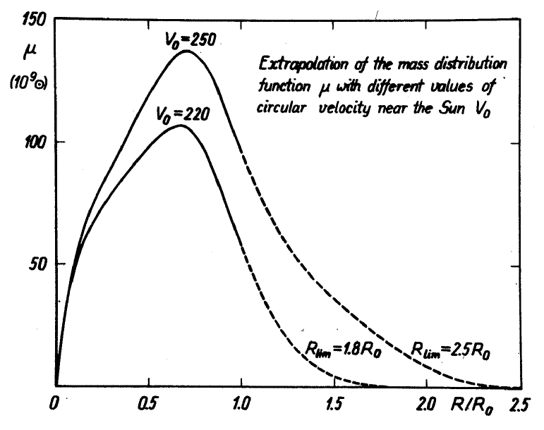
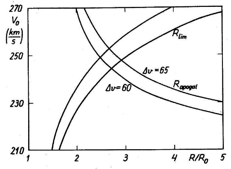
Figure 1: Left: The extrapolation of the mass distribution function beyond the Sun’s distance $R>R_{0}$ (dashed lines) with different values for the circular velocity near the Sun, $V_{0}$. Limiting radii of models, $R_{lim}$, are indicated. Right: The dependence of limiting radii, $R_{lim}$, and apogalactic distances, $R_{apogal}$, on circular velocity near the Sun, $V_{0}$. Two cases of smooth extrapolation of the mass distribution function with different $R_{lim}$ are indicated. Apogalactic distances are given for two values of Oort’s limiting velocity, $\Delta\,v$.

As recognised by Strömberg (1924) and Oort (1928), no stars with apices within Galactic longitudes $l=20^{\circ}-85^{\circ}$ and heliocentric velocities exceeding 65 km/s are found. The limiting velocity may correspond to the velocity required to reach the boundary of the Galaxy (Bottlinger 1933), or to the velocity of escape (Oort 1928). As shown by Kuzmin (1956b), only the first alternative, $R_{apogal}=R_{lim}$, can be correct. Adopting the second alternative, as done by Schmidt (1956), we get $R_{lim}\ll R_{apogal}\approx\infty$, but this situation is impossible since stars with velocities smaller than the escape velocity belong to the system and must be included into the mass distribution function. If these stars are included to the model, we get

$$R_{lim}=R_{apogal}.$$ (9)

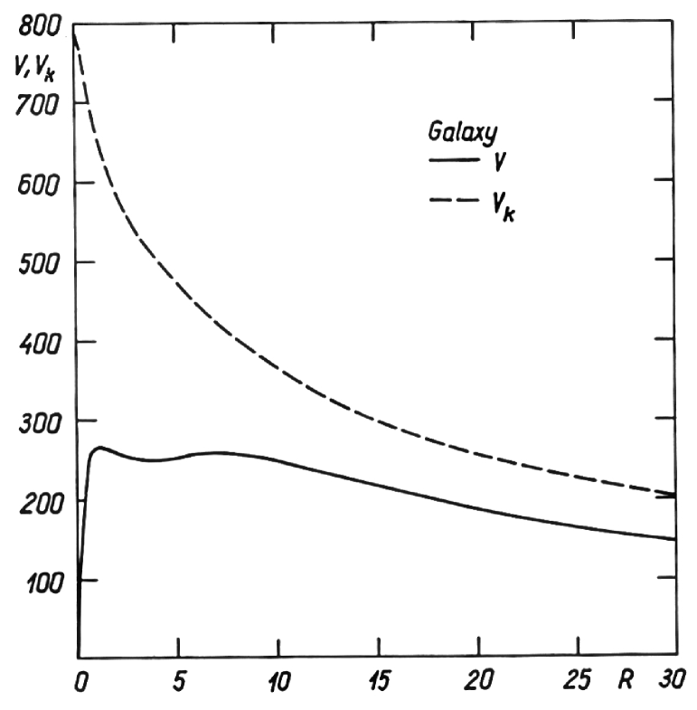
Figure 2: Circular and escape velocities as functions of distance from Galactic centre.

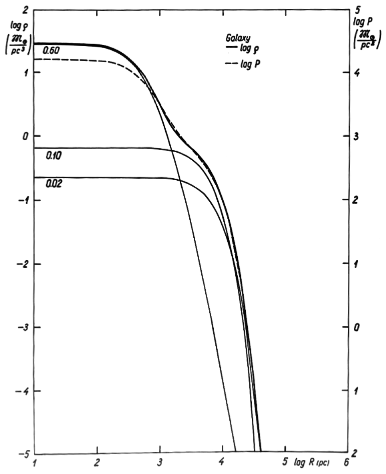
Figure 3: Spatial densities $\rho$, and projected densities $P$ of components as functions of distance from Galactic centre.

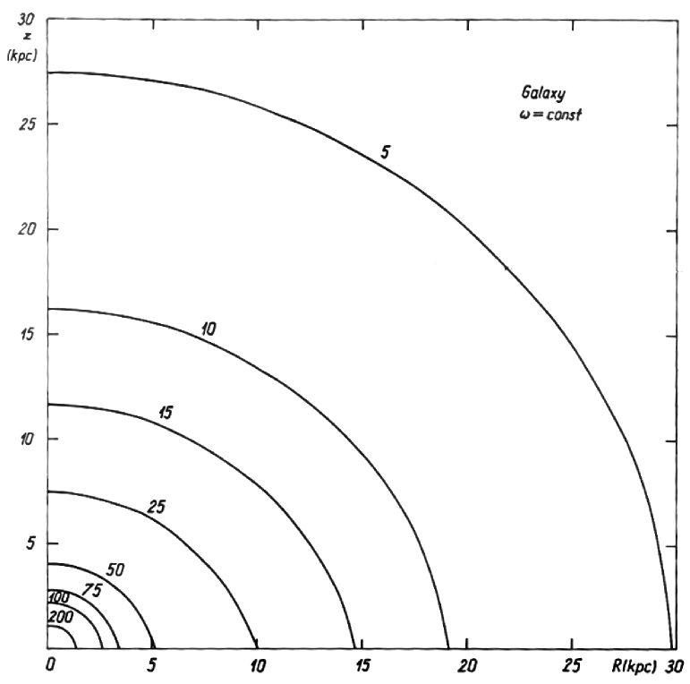
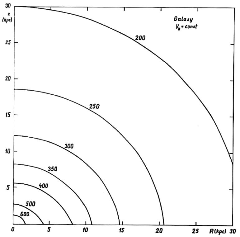
Figure 4: Isolines of angular velocity $\omega_{0}$ and escape velocity $V_{k}$ are shown in left and right panels, respectively

Table 4: Parameters of test components of the Galaxy

Popul.	$\epsilon$	$a_{0}$	$N$	$x_{0}$	$(\sigma_{z})_{0}$	$\sigma_{z}$	$\sigma_{R}$	$V_{\theta}$	$t$
		kpc				km/s			$10^{9}$yr
Flat	0.02	8.0	0.5	0.0	8.8	8.8	16.4	250	0.9
Disc 1	0.05	7.4	1.0	1.5	20.4	19.9	37.3	239	3.9
Disc 2	0.10	6.4	1.5	3.0	34.7	34.4	64.5	216	7.6
Halo 1	0.20	4.5	2.0	4.5	52.8	51.7	84.3	185	9.1
Halo 2	0.40	1.9	3.0	7.5	75.2	71.4	92.8	142	9.4
Halo 3	0.60	0.9	4.0	10.5	92.6	85.9	100.9	96	9.7
Halo 4	0.80	0.6	5.0	13.5	108.3	98.5	109.8	46	10.0

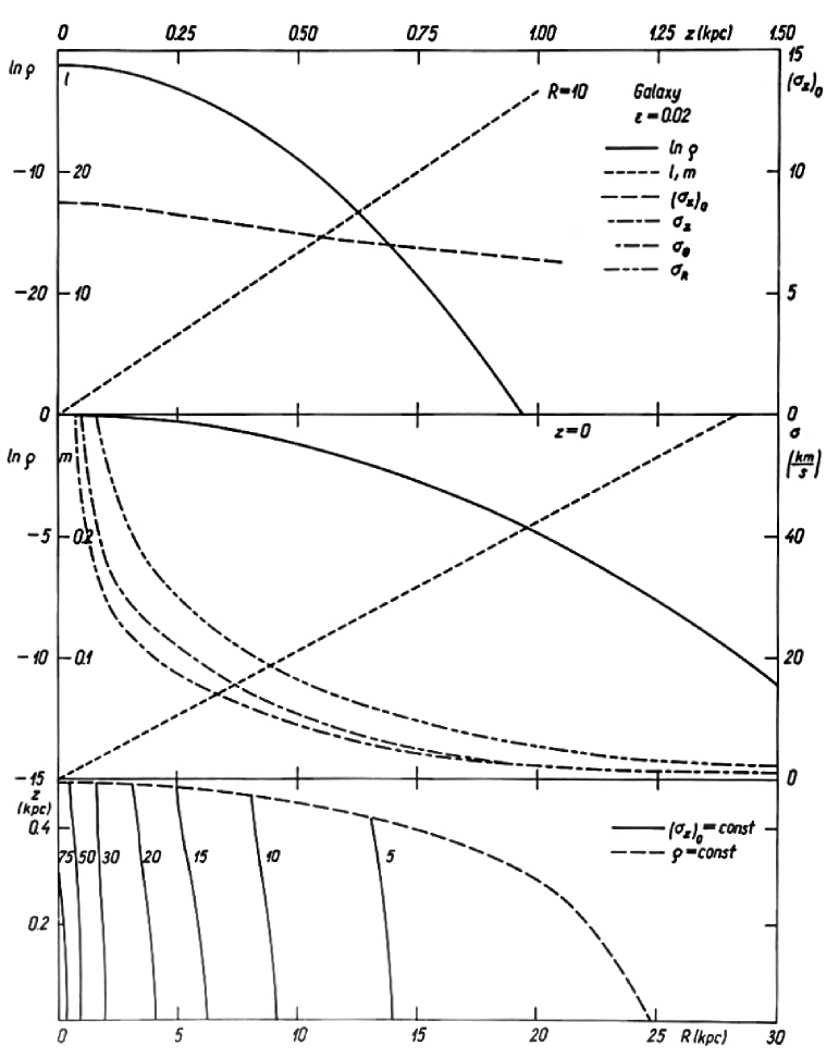
Figure 5: Descriptive functions for the test population of flattening $\epsilon=0.02$.

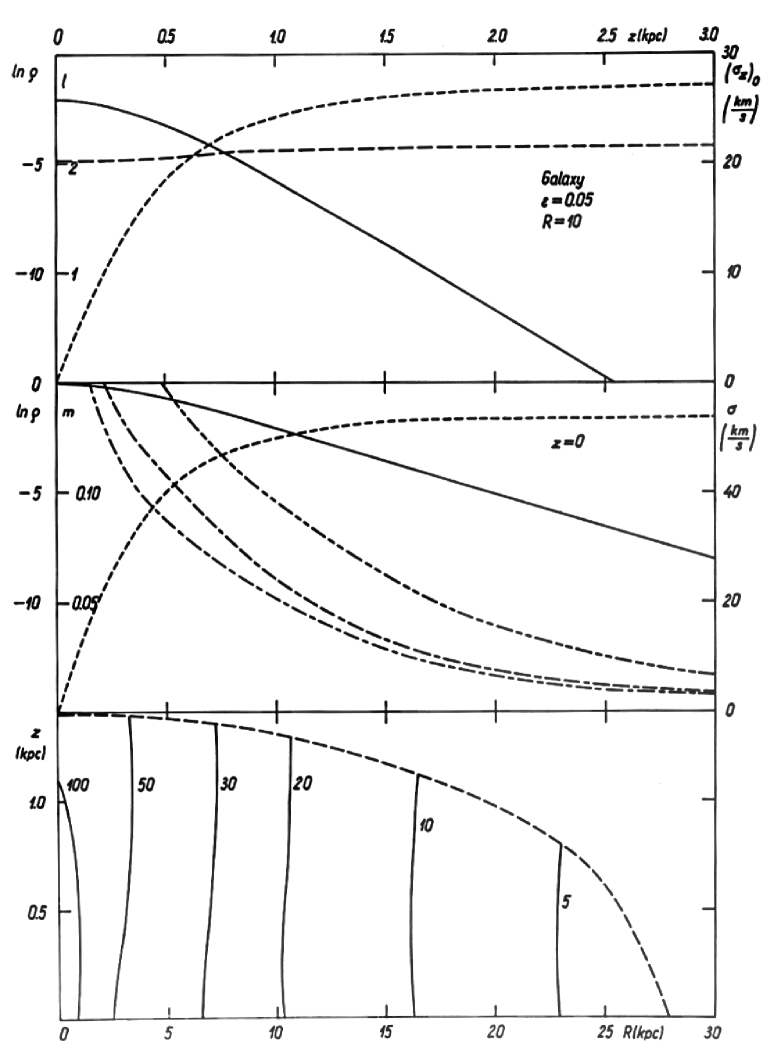
Figure 6: Descriptive functions for the test population of flattening $\epsilon=0.05$.

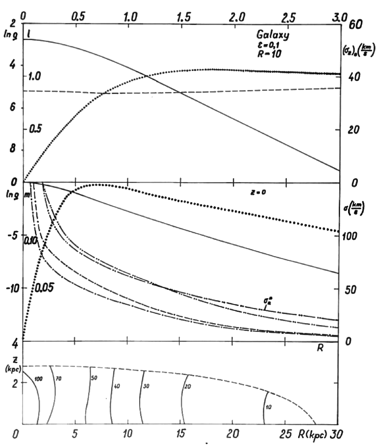
Figure 7: Descriptive functions for the test population of flattening $\epsilon=0.10$.

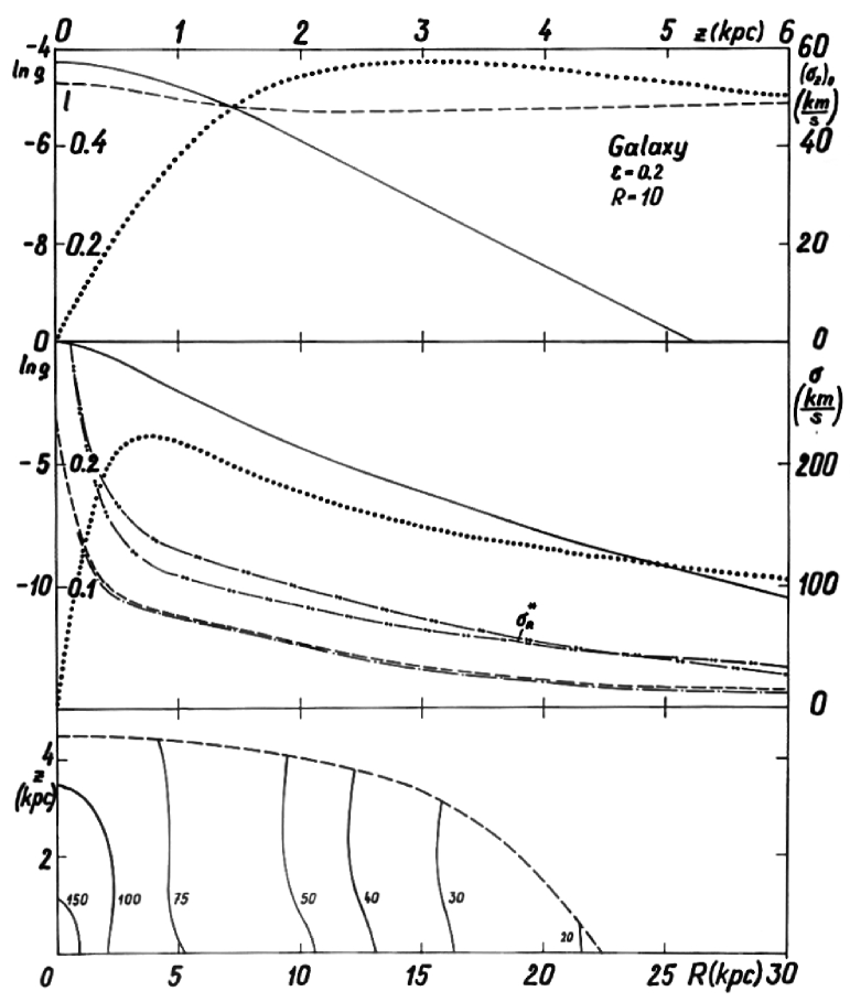
Figure 8: Descriptive functions for the test population of flattening $\epsilon=0.20$.

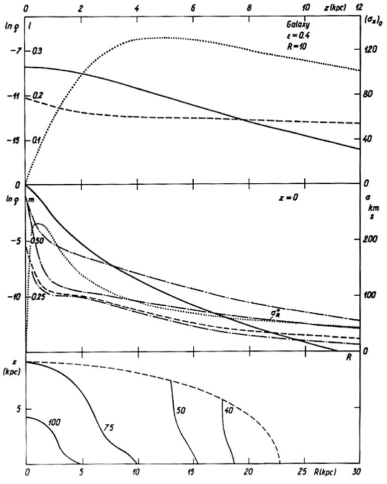
Figure 9: Descriptive functions for the test population of flattening $\epsilon=0.40$..

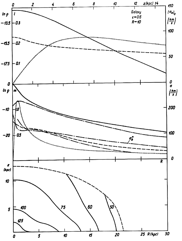
Figure 10: Descriptive functions for the test population of flattening $\epsilon=0.60$.

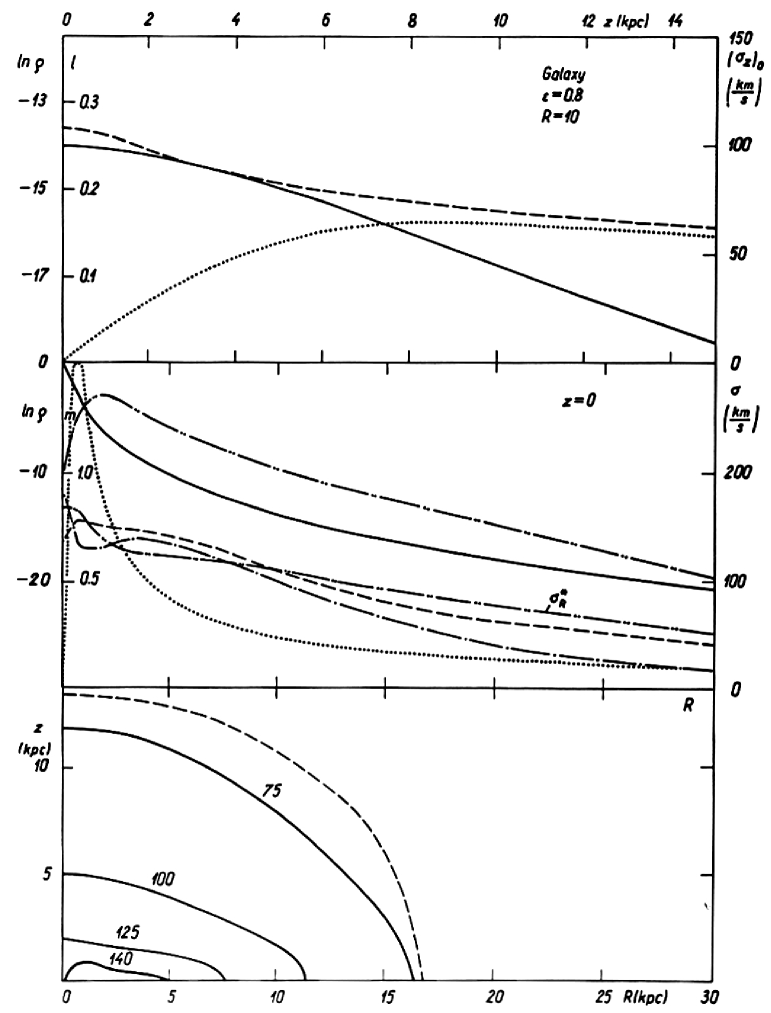
Figure 11: Descriptive functions for the test population of flattening $\epsilon=0.8$.

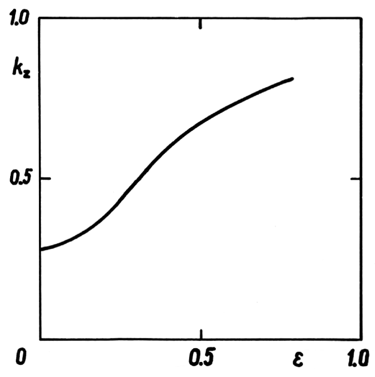
Figure 12: The dependence of $k_{z}=\sigma_{z}^{2}/\sigma_{R}^{2}$ on $\epsilon$ at $R=10$ kpc and $z=0$.

In left panel of Fig. 1 the mass distribution function, $\mu(a)$, is given for two values of the circular velocity, $V_{0}$. In both cases, the function of differential rotation, $U(x)$, is the same, and the extrapolation of $\mu(x)$ beyond the Sun’s distance, $R>R_{0}$, is smooth. In right panel of Fig. 1 the dependence of $R_{lim}$ and $R_{apogal}$ on $V_{0}$ is shown.

Both methods, the use of the gradient of spatial density and Oort’s limiting velocity, give the circular velocity values $V_{0}\approx 250$ km/s (Kuzmin 1956b). These possibilities for checking the circular velocity were mentioned by Schmidt (1965). But in respect of extrapolation of the mass distribution function, his new model is overcorrected, as $R_{lim}>R_{apogal}$. The cause is a too low decrease of the mass density in outer regions of the model according to power law $\rho\propto a^{-4}$. The same behaviour has the model constructed by Takase (1967).

For our Galaxy, we have no direct argument against the power law $\rho\propto a^{-4}$ and $R_{lim}>R_{apogal}$. Photometric observations of other galaxies show, however, that galaxies have well-defined outer boundaries (Arp & Bertola 1971) with exponential density law (de Vaucouleurs 1969). If we accept for density the power law $\rho\propto a^{-4}$, and for the circular velocity the Bottlinger (1933) profile as in the model by Takase (1967), then with increasing $a$ the mass-to-light ratio becomes very great, which is difficult to accept. On the other hand, if we accept $R_{lim}>R_{apogal}$, then in peripheral regions of the Galaxy, all stars have small velocity dispersion, and no such stars can reach in their orbits the Solar region. Data on other galaxies suggest that peripheral regions of galaxies belong to halo population with large velocity dispersion. For these reasons, it is not likely that among these halo stars there are none with $R_{perigal}\leq R_{0}$.

The structure of the inner parts of models was discussed in detail by Einasto (1965). Here we shortly discuss new models, suggested after the publication of the model by Einasto (1965).

One of aspects of the structure of galaxies is the presence of a dense nucleus. To describe this aspect of the structure of the Galaxy, Schmidt (1965) and Innanen (1966a) used density laws with infinite density at centre. It is clear that in this region their models have only the approximate meaning. Such models have the peculiarity having zero velocity dispersion at the very center. This aspect was ignored by Innanen & Kellett (1968), where velocity dispersions were estimated for the Innanen (1966a) model. Presently we have little information on the density of matter near the centre of the Galaxy. Available data are probably underestimates.

3 A new model of Galaxy

We suppose that the mass distribution of the Galaxy can be represented by a sum of three ellipsoidal components with various axial ratios $\epsilon$. One ellipsoid represents spherical populations (halo and bulge), the second ellipsoid represents the disc, and the third one the flat component.

For mass density distribution of components of the Galaxy, we use the modified exponential profile:

$$\rho(a)=\rho_{0}\,\exp[x_{0}-(x_{0}^{2N}+\xi^{2})^{1/(2N)}],$$ (10)

where

$$\rho_{0}={\mathfrak{M}\,\over a_{0}^{3}}{h\over 4\pi\epsilon}$$ (11)

is the central density, and

$$\xi=a/(k\,a_{0}),\hskip 28.45274pta^{2}=R^{2}+z^{2}/\epsilon^{2}.$$ (12)

Here $\mathfrak{M}\,$ is the mass of the components, $a_{0}$ is its harmonic mean radius, defined by the formula

$$a_{0}^{-1}=\mathfrak{M}\,^{-1}\int_{0}^{\infty}\mu(a)\,a^{-1}{\rm d}a\,,$$ (13)

and $N$ and $x_{0}$ are structural parameters. $h$, $k$ are dimensionless normalising parameters needed to get for the mass and harmonic mean radius definition formulae Eq. (13) and

$$\mathfrak{M}\,=\int_{0}^{\infty}\,\mu(a){\rm d}a\,,$$ (14)

as suggested by Einasto (1968d). We use the harmonic mean radius $a_{0}$ is the effective radius of the model. The parameter $x_{0}$ is introduced to avoid a too sharp density peak and the resulting minimum in velocity dispersion near the centre of the model. If we take $x_{0}=0$, we get the exponential density profile as suggested by Einasto (1965):

$$\rho(a)=\rho_{0}\,\exp[-\xi^{1/N}].$$ (15)

We adopted structural parameters of components on the basis of analogy with the Andromeda galaxy (Einasto 1969b, 1970c). The spherical component combines halo and bulge populations, which for M31 had $\epsilon=0.30$ and $\epsilon=0.80$, respectively. For Galaxy we used an intermedium value $\epsilon=0.6$. For disc and flat components we used $\epsilon=0.10$ and $\epsilon=0.02$. These components represent actual populations in the flatness range $0.05\leq\epsilon\leq 0.20$ and $\epsilon<0.05$.

The mean radius of spherical component was determined using photometric data by Arp & Bertola (1971) on the bulge of Galaxy, and data by Perek (1962) on the distribution of RR Lyrae variables. The mass of this component was determined using the rotation velocity in inner parts of the Galaxy (Schmidt 1965). Mean radii and masses of other two components were estimated on the basis of available data on the distribution of disc population and young stars. The final values were found by a trial-and-error procedure to have at $R=R_{0}$ the adopted values of Oort-Kuzmin parameters. Parameter $x_{0}$ was found by a similar procedure to have a monotonous increase of the velocity dispersion by decreasing $a_{0}$. The adopted parameters are given in Table 2.

We calculated for our model all principal descriptive functions. For the Galactic plane $z=0$ we found: Oort-Kuzmin parameters $A,\leavevmode\nobreak\ B,\leavevmode\nobreak\ C$, angular velocity $\omega_{0}$, circular velocity $V_{c}$, escape velocity $V_{k}$, and ratios of velocity dispersions $k_{\theta}$ and $k_{z}$. These data are given in Table 3. Circular velocity and escape velocity as functions of distance from the Galactic centre are shown in Fig. 2. Spatial densities $\rho$ and projected densities $P$ of components are shown in Fig. 3. Isolines of angular velocity $\omega_{0}$ and escape velocity $V_{k}$ are given in Fig. 4.

A few comments on the results obtained. Of special interest is the angular velocity $\omega_{0}$. It was calculated using the first hydrodynamical equation by Einasto & Rümmel (1970b), see Chapter 11, which for small velocity dispersion, $\sigma_{R}\rightarrow 0$, has the form

$$V_{\theta}^{2}=R\,K_{R}=V_{c}^{2},$$ (16)

where $K_{R}=-\partial\Phi/\partial R$, and $\Phi$ is the gravitational potential. On the $z=0$ surface $\omega_{0}=V_{c}/R$, where $V_{c}$ is circular velocity. Fig. 4 shows that in the $R,z$ surface isolines of $\omega_{0}$ are slightly flattened ellipsis. From the theory of stationary galaxies it follows that isolines of $\omega_{0}$ should be spheres (Kuzmin 1956b). Assumptions of stationary galaxies are not exact, thus, small deviations from spheres are likely.

When we compare description functions of our Galaxy with similar functions for the Andromeda galaxy (Einasto & Rümmel 1970b), we see that they are very similar. The only large difference is in the structure of central regions. Presently we have little data on the structure of the nucleus of the Galaxy. For this reason, the nucleus was not included as a component. Available data suggest that the nucleus of the Galaxy is similar to the nucleus of M31. If this is correct, then the central density of the Galaxy would be of the order $10^{6}\,M_{\odot}pc^{-3}$, and the velocity of escape about 1500 km/s, i.e.  two times higher than adopted in the present model. To understand the structure of the central regions of the Galaxy, new observational data are needed.

4 Kinematics of population

We used the model to find various characteristics of the spatial and kinematical structure of test populations. These test populations are listed in Table LABEL:Tab7.4, they represent various actual Galactic populations. The following data are listed: flattening $\epsilon$, effective radius $a_{0}$, structural parameters $N$ and $x_{0}$, normalising parameter $k$, vertical velocity dispersion $(\sigma_{z})_{0}$ at the Sun distance in Jeans approximation, vertical velocity dispersion $\sigma_{z}$ at the Sun distance, radial velocity dispersion $\sigma_{R}$ at Sun distance, rotational velocity $V_{\theta}$ at Sun distance, and estimated age $t$.

For test populations, we calculated various descriptive functions, shown in Figs. 5 to 11. These Figures have three panels.

In the upper panel, we show with solid lines the density logarithm, $\ln\rho$, with dotted lines the vertical density gradient, $l=-\partial\log\rho/\partial z$, and with dashed lines the velocity dispersion $(\sigma_{z})_{0}$ in Jeans approximation, see Chapter 11. Velocity dispersion $(\sigma_{z})_{0}$ was calculated within the range $0\leq z\leq z_{u}$, where $z_{u}$ is the outer vertical limit of the population. All functions are plotted as functions of $z$ at $R=10$ kpc, the adopted distance of the Sun from Galactic centre. The vertical scale $z$ is shown at the top of the panel, the density scale is on the left border, and the velocity dispersion scale on the right border.

Central panels of Figures show with solid lines the logarithm of the density, $\rho$, with dotted lines radial density gradient, $m=-\partial\log\rho/\partial R$, and with various dot-dashed lines velocity dispersions $\sigma_{R},\leavevmode\nobreak\ \sigma_{\theta},\sigma_{z}$. These data are given as functions of $R$ on the plane of the Galaxy, $z=0$. The radial distance scale $R$ is shown at the lower border of the Figure, the density scale is on the left vertical border, and the velocity dispersion scale on the right border. Densities are given in units of the central density, gradients $l$ and $m$ in kpc^-1, dispersions in km/s. Vertical velocity dispersions $\sigma_{z}$ were calculated from the second hydrodynamical equation (5), using for $k_{z}$ Kuzmin equation (4) from the theory of irregular forces. Radial velocity dispersions $\sigma_{R}$ were found from definition equation (8) from $\sigma_{z}$ and $k_{z}$, taking into account the Kuzmin equation (4). For the test populations with $\epsilon\geq 0.10$ radial velocity dispersions were also calculated from the first hydrodynamical equation (4) from circular velocity $V_{c}$ and rotational velocity $V_{\theta}$, this dispersion is marked as $\sigma_{R}^{\ast}$. Figs. 7 – 11 show that in disc populations both versions of the radial velocity dispersion are very similar, but in halo populations $\sigma_{R}$ is larger than $\sigma_{R}^{\ast}$.

In bottom panels we show with dashed lines isolines, $\rho=const$ and with solid lines isolines $(\sigma_{z})_{0}=const$, in the plane of $R,\leavevmode\nobreak\ z$-coordinates, shown at the bottom and the left border of the panel. Velocity dispersion $\sigma_{z}$ was calculated within ranges $0\leq R\leq 30$ kpc and $0\leq z\leq z_{u}$, where $z_{u}$ is the outer vertical limit of the population. We see that in disc populations lines $(\sigma_{z})_{0}=const$ are vertical, i.e. the velocity dispersion at given radial distance is constant. In halo populations lines $(\sigma_{z})_{0}=const$ are similar to lines of constant density. A similar picture is observed in the M31 galaxy, see Fig. 10.

Now we discuss our results in some detail.

Velocity dispersions of disc populations have maxima at center and decrease with the distance from the Galactic center. In halo populations velocity dispersions near the center have a moderate minimum, a maximum not far from the center, and decrease at larger distance. The radial density gradient is zero at $R=0$, and increases continuously with increasing distance for disc populations, $\epsilon=0.02,\leavevmode\nobreak\ 0.05$. For halo populations the gradient has a maximum at certain distance from the center, and slowly decreases at larger distance.

A remarkable property is the form of isolines of vertical velocity dispersion $\sigma_{z}=const$. Outside central regions of the Galaxy, isolines of velocity dispersion of flat and intermediate populations are almost vertical, i.e.  velocity dispersions depend very weakly on $z$. Available observational data support this picture. A different picture was obtained by Innanen & Kellett (1968). Velocity dispersion isolines for his model (Innanen 1966a) were almost parallel to density isolines $\rho=const$, i.e.  velocity dispersion $\sigma_{z}$ rapidly decrease with the increase of $z$. The reason for this discrepancy between models is the Schmidt density law with a sharp boundary, accepted by Innanen.

On the $z=0$ surface, we can take into account corrections to $\sigma_{z}$, using the gradient of the tilt of the velocity ellipsoid. Applying equations from Chapter 11, we have in the Jeans approximation

$$Q^{\star}(\sigma_{z}^{2})_{0}=R^{2}\,C^{2},$$ (17)

where $C$ is the dynamical Kuzmin constant, $(\sigma_{z})_{0}$ — the vertical velocity dispersion in Jeans approximation, and

$$-Q^{\star}=R^{2}\left({\partial^{2}\ln\sigma_{z}^{2}\over\partial z^{2}}+{\partial^{2}\ln\rho\over\partial z^{2}}\right).$$ (18)

Taking into account the gradient of the tilt of the velocity ellipsoid, we get

$$Q\sigma_{z}^{2}=R^{2}\,C^{2},$$ (19)

where

$$Q=Q^{\star}-q^{\prime},$$ (20)

and $q^{\prime}$ is given by the Eq. (29). In calculations, we used $Q^{\star}$ not from Eq. (18) but from Eq. (17), since $(\sigma_{z})_{0}$ is already known. Parameter $q^{\prime}$ was calculated using Eq. (29). Results of calculations are given in upper panels of Figs. 5 to 11. We see that the tilt of velocity ellipsoid decreases velocity dispersions slightly. Near the axis of the system $R=0$, this factor increases the velocity dispersion. In this way, according to the virial theorem, the mean value of the dispersion does not change.

The first hydrodynamical Eq. (1) is usually applied to calculate the centroid velocity, $V_{\theta}$, from the velocity dispersion, $\sigma_{R}$. The last quantity is calculated using the definition equation

$$k_{z}={\sigma_{z}^{2}\over\sigma_{R}^{2}},$$ (21)

from $\sigma_{z}$ and $k_{z}$. The vertical dispersion can be found from the second hydrodynamical Eq. (2), and $k_{z}$ from Eq. (26) and Eq. (11).

This method of finding $\sigma_{R}$ gave satisfactory results only for flat populations. The higher the velocity dispersion, the more the calculated centroid velocity differs from the observed one. Starting from some $\sigma_{R}$, the pressure component of the hydrodynamical equation becomes larger than the right part of the equation, and the centroid velocity becomes imaginary. This absurd result shows that we have made an error in our calculations.

This hydrodynamical equation can be written in the form Eq. (4)

$$V_{\theta}^{2}-p\,\sigma_{R}^{2}=V_{c}^{2},$$ (22)

where the dimensionless coefficient $p$ has on the symmetry plane of the galaxy the form Eq (19). Initially, we suspected that the non-correct result was caused by the wrong calculation of the coefficient $p$. However, a careful analysis brought us to the conclusion that non-accuracy in the calculation of $p$ cannot be so large to bring us to such an absurd result. It remains to check the correctness of the determination of the dispersion $\sigma_{R}$.

As written above, we calculated the dispersion $\sigma_{R}$ using Eq. (21). The vertical dispersion $\sigma_{z}$ is determined accurately. There remains to search the error in the coefficient $k_{z}$. It was calculated using the Kuzmin Eq. (26), which was defined only for flat populations.

In the Solar neighbourhood, the dispersion $\sigma_{R}$ can be calculated directly using Eq. (22), since $V_{\theta}$ can be found from observations, and the coefficient $p$ calculated either from observational data or from model. In the latter case, the Eq. (19) is applied. The obtained dispersion $\sigma_{R}$ was used to adjust $k_{z}$ using Eq. (21).

The relationship between the velocity dispersion and the centroid velocity was determined using the mean velocity dispersion $\sigma$. Thus, we need a relationship between the mean dispersion $\sigma$ and the dispersion in the radial direction $\sigma_{R}$. It has the form

$$\sigma_{z}^{2}={3k_{z}\over 1+k_{\theta}+k_{z}}\,\sigma^{2}.$$ (23)

The coefficient $k_{\theta}$ was calculated from the relation

$$\left({1-k_{\theta}\over 1-k_{z}}\right)=\left({1-k_{\theta}\over 1-k_{z}}\right)_{0},$$ (24)

where index 0 is for $k_{\theta}$ and $k_{z}$ on the plane of the population.

To determine the dispersion $\sigma_{R}$, another method can be used, which applies the first hydrodynamical equation as a differential equation for $\sigma_{R}$. To solve this task, we need to express $V_{\theta}$ as a function of $R$. We are interested in solving this equation for spherical populations, which have low rotational velocities, $V_{\theta}\ll V$. Since $V_{\theta}$ is low, small non-accuracies in this quantity do not influence our result. Thus we accepted

$$V_{\theta}(R)=\beta\,V_{c}(R),$$ (25)

where $\beta$ is a parameter, constant for a given population. Its value can be estimated from kinematical data of populations near the Sun. The solution of the first hydrodynamical equation can be written in the form

$$\sigma_{R}^{2}(R)=\alpha\int_{R}^{\infty}K_{R}(R^{\prime}){\rho(R^{\prime})\over\rho(R)}{L(R^{\prime})\over L(R)}{\rm d}R^{\prime}\,,$$ (26)

where

$$\alpha=1-\beta^{2}$$ (27)

and

$$L(R)=\exp\left[-\int_{R}^{R1}p(R^{\star}){{\rm d}R^{\star}\,\over R^{\star}}\right].$$ (28)

Here $R1$ is a certain distance which later disappears, and

$$p(R)=(1-k_{\theta})+n_{R}(1-k_{z}),$$ (29)

where $n_{R}$ is expressed by Eq. (21). If we take $p=0$, then $L=1$ and we get the velocity dispersion in Jeans approximation. We calculated $\sigma_{R}$ for $p=0$ and for $p$ according to Eq (29).

Results of these calculations are shown in Figs. 5 to 11. These results show, first, that the radial velocity dispersion of populations is not constant as expected from the theory, using the assumption that the ellipsoidal distribution of velocities is fulfilled accurately. Furthermore, our results show that ratios of velocity dispersions depend on dispersion. If the dispersion is small, then $k_{z}$ approximates to the value given by Kuzmin equation. When the dispersion increases, then $k_{z}$ also increases, see Fig. 12. Such a result is expected, since iso-surfaces of densities approach spheres, which in the limit approach spheres, determined by the escape velocity.

5 Density distribution of populations

For all test populations, we calculated spatial densities in meridional surfaces $R,z$, projected densities $P$, and density gradients in radial and vertical directions.

Consider first the density distribution in radial directions. Density gradients near the Sun,

$$m=-{\partial\log\rho\over\partial R},$$ (30)

are close to values expected from observations (Kukarkin 1949; Parenago 1954b; Blaauw & Schmidt 1965). In central regions of the Galaxy, the density gradient $m$ of the halo populations is much larger than near the Sun. This is in good agreement with results by Baade (1958) for the Galaxy and Sharov (1968a, c) for M31. This agreement demonstrates that our test population model and its scale parameters were chosen properly.

The vertical density distribution is often accepted according to an exponential law (Kukarkin 1949; Parenago 1954b)

$$\rho(z)=\rho_{0}\,\exp^{-|z|/\beta},$$ (31)

where $\beta$ is a parameter, inversely proportional to the gradient of density logarithm,

$$\beta^{-1}Mod=l=-{\partial\log\rho\over\partial z}.$$ (32)

If the density behaves according to Eq. (31), then the gradient $l$ should be constant.

Our calculations show that the gradient is not constant. This shows that Eq. (31) can be used only as the first approximation. Density gradients found in this paper describe well the observed distributions of stars. We cannot expect a full coincidence, since the observed populations of stars are not completely homogeneous but consist of several close populations with slightly variable properties, for instance, sums of several our close test populations.

September 1971

Part 2 Methods to calculate spatial and hydrodynamical models of regular stellar systems

Chapter 9 Classification of models. Conditions of physical correctness

The usual method to describe the structure of galaxies quantitatively is to construct respective mathematical models. A review of models of galaxies is given by Perek (1962). A more detailed discussion of modelling methods is made by Kutuzov & Einasto (1968), which forms Chapter 8 of the original Thesis. In this English version, we describe one aspect of the calculation of models — conditions of physical correctness.

In general, models of galaxies can be characterised as spatial/hydrodynamical, theoretical/empirical, general/detailed. Theoretical models are devoted to explaining particular theoretical properties, such as the model by Kuzmin (1952c, 1954) to explain the third integral of motions. Examples of empirical spatial models are models of the Galaxy by Idlis (1956), Schmidt (1956) and Einasto (1965). An example of a hydrodynamical model is the model of M31 by Einasto & Rümmel (1970b).

The conditions of physical correctness can be expressed in the following way (Einasto 1969a):
(a) the spatial density $\rho(a)$ must be non-negative and finite,

$$0\leq\rho(a)<\infty;$$ (1)

(b) the density should decrease with growing distance from the centre of the system:

$$G\{\rho(R)\}=\frac{\partial\ln\rho}{\partial\ln R}\leq 0;$$ (2)

(c) the descriptive functions should not have breaks;
(d) some moments of the mass-function should be finite:

$$\mathfrak{M}\,_{i}=\int_{0}^{\infty}{\mu(a)\,a^{i}{\rm d}a\,}<\infty,$$ (3)

where $\mu(a)=4\pi\epsilon\rho(a)\,a^{2}$ is the mass function;
(e) the model should allow stable circular motions. In that case

$$G\{F_{R}^{0}(R)\}=\frac{\partial\ln F^{0}_{R}}{\partial\ln R}>-1.$$ (4)

Here $F_{R}^{0}(R)=F_{R}(R)/\mathfrak{M}\,$ is the normalised acceleration function – the ratio of radial acceleration of the model to the radial acceleration of a mass-point model with the same mass $\mathfrak{M}\,$. For a mass point $F_{R}^{0}(R)\equiv 1$.

Real stellar systems have finite dimensions and finite densities. Therefore, all moments of the mass function, $\mathfrak{M}\,_{i}$, $i\geq-2$, are finite. But the requirement of the finiteness of all moments is too strict. Therefore, we suppose that only moments of the order, $-2\leq i\leq 2$, must be finite. Moments $\mathfrak{M}\,_{-1}$ and $\mathfrak{M}\,_{0}$ determine the central potential and the mass of the model, respectively. Moment $\mathfrak{M}\,_{1}$ defines the effective radius of the model, see Eq. (13).

July 1969

Chapter 10 Description functions and parameters

The problem of constructing an empirical model of a particular stellar system consists of fixing description functions and determination of their parameters. The aim of this paper is to discuss description functions and parameters of stellar systems and their models in general terms. The full text of this Chapter is published by Einasto (1968a). We here give a short summary of the main points.

We assume in galactic modelling that galaxies consist of a sum of ellipsoidal components of axial symmetry around the $z$-axis, and that all components have the identical symmetry plane $z=0$. Components have the vertical to radial axis ratio: $\epsilon=c/a$, where $c$ is the minor semiaxis of the density ellipsoid, and $a$ is the major semiaxis of the density ellipsoid: $a^{2}=x^{2}+y^{2}+(z/\epsilon)^{2}$.

The main description functions for Galactic modelling are the following:
         $\rho(a)$ — spatial density of mass;
         $\mu(a)$ — mass function;
         $P(a)$ — projected mass density (definition below);
         $l(a)$ — spatial luminosity density;
         $L(R)$ — projected luminosity density;
         $V(R)$ — circular velocity.
In these equations, $a$ is the major semiaxis of the equal density ellipsoid, and $R$ is the radial distance from the centre of the galaxy.

Description functions are connected by the following equations: the mass function,

$$\mu(a)=4\pi\epsilon\rho(a)\,a^{2},$$ (1)

the projected density function,

$$P(A)={1\over 2\pi\,E}\int_{A}^{A^{\circ}}{\mu(a)\,{\rm d}a\,\over a\,\sqrt{a^{2}-A^{2}}},$$ (2)

here $A$ is the major semiaxis of the projected density,

$$A^{2}=X^{2}+E^{-2}\,Y^{2},$$ (3)

where $E=\epsilon/A$ is the axial ratio of the projected density ellipsoid. The projected and spatial density ellipsoid axial ratios are related as;

$$E^{2}=cos^{2}i+\epsilon^{2}\,sin^{2}i,$$ (4)

where $i$ is the inclination angle of the symmetry axis of the galaxy to the line of sight.

Spatial mass and luminosity densities are related as:

$$\rho(a)=f\,l(a),$$ (5)

where $f$ is the mass-to-light ratio of a given component.

The circular velocity is related with the mass function as follows:

$$V(R)^{2}=G\int_{0}^{R}\frac{\mu(a)\leavevmode\nobreak\ da}{\sqrt{R^{2}-a^{2}e^{2}}},$$ (6)

where $G$ is the gravitational constant, and $e^{2}=1-\epsilon^{2}$. In these equations, we assume that the stellar system can be divided into a number of homogeneous components, each with its axial ratio $\epsilon$ and mass-to-light ratio $f=\rho(a)/l(a)=P(A)/L(A)$.

The descriptive parameters of stellar systems and their models can be divided into three groups:

a) the model-parameters — parameters in the analytical expressions of descriptive functions in the special models of stellar systems;

b) the gross-parameters — integral quantities, characterising the structure of a stellar system as a whole;

c) the local galactic parameters — values of the galactic descriptive functions or their combinations for the surrounding of the Sun.

The model- and gross-parameters can be divided into three kinds of parameters: scale-, concentration-, and flattening parameters, the latter two kinds of parameters can be called together as the structural ones. There are two scale parameters, one of them determines the scale of the model in the space, the other the scale of the density (or the mass). The concentration and flattening model-parameters determine the concentration of mass to the centre of the model and the form of the equidensity surfaces.

The gross-parameters are defined by means of the moments of the mass-function, $\mu(a)$. It is proposed to use the effective radius, $R_{e}$, and the mass, $\mathfrak{M}\,$, of the system as scale gross-parameters. A dimensionless concentration gross-parameter is the index $\nu$ in the generalised exponential model, Eq. (4). Dimensionless flattening parameter is the axial ratio of equidensity ellipsoid $\epsilon$.

In practical use, it is common to accept mass functions of components using suitable approximation density profiles, and to find the circular velocity from Eq. (6) by summing the contribution of all components.

April 1967

Chapter 11 Calculation of models of spatial structure

In previous papers in this series, I discussed the classification of stellar system models, the description functions and parameters of models, and the type of relations between the description functions. This article is devoted to the methodology of model building. In this case, the model of a stellar system is defined as a collection of mass or luminosity distribution functions, constructed for a particular stellar system and given in a numerical form. We assume that the stellar system has axial and planar symmetry, and that it consists of a finite number of physically homogeneous spheroidal components. The full text of the Chapter is published by Einasto (1968d). Here we give a short summary.

The basic input data to find a composite model of a galaxy are luminosity distributions of components, and in some cases rotation velocities of components. The total luminosity distribution of the galaxy is the sum of distributions of its components:

$$L(X,Y)=\sum_{k=1}^{n}{L_{k}(A_{k})},$$ (1)

where $n$ is the number of components,

$$A_{k}^{2}=X^{2}+E_{k}^{-2}\,Y^{2},$$ (2)

is the major semiaxis of the projected equidensity ellipse, $X$ and $Y$ are rectangular projected coordinates, and

$$E_{k}^{2}=cos^{2}\,i+\epsilon_{k}^{2}\,sin^{2}\,$$ (3)

is the axial ratio of the projected density ellipsoid of the component, and $i$ is the inclination angle of the symmetry axis of the galaxy to the line of sight. The projected luminosity distribution is related to the spatial mass function as follows:

$$L_{k}(A_{k})={1\over 2\pi\,E_{k}}\int_{A_{k}}^{A^{\circ}}{\mu_{k}(a)\,{\rm d}a\,\over f_{k}\,a\,\sqrt{a^{2}-A_{k}^{2}}},$$ (4)

where

$$\mu_{k}(a)=4\pi\epsilon_{k}\rho_{k}(a)\,a^{2},$$ (5)

is the mass function of the component $k$, $f_{k}$ is the mass-to-light ratio of the components, and $\epsilon_{k}$ is the axial ratio of its spatial density ellipsoid.

Similarly, the total velocity function is a sum of circular velocity functions of components:

$$V(R)^{2}=\sum_{k=1}^{n}{V_{k}(R)^{2}},$$ (6)

where the circular velocity function of components is:

$$V_{k}(R)^{2}=G\int_{0}^{R}\frac{\mu_{k}(a)\leavevmode\nobreak\ da}{\sqrt{R^{2}-a^{2}e_{k}^{2}}}.$$ (7)

The task of modelling a stellar system is to calculate from the available observational data all necessary functions and parameters to describe a stellar system. The modelling procedures vary widely depending on the availability of observational material, on the way of solving the main integral equations (4) and (7), and the resulting form of model representation. The procedures of extrapolating and interpolating the observed description functions are quite different. All these aspects allow further methodological refinement and specification in the classification of the models, proposed by Einasto (1968a).

Let us now consider in a little more detail some aspects of stellar system modelling.

A. It is well known that in the case of stellar systems visible from the outside, observations allow to determine:

1) the projected luminosity distribution function $L_{S}(X,Y)$ in photometric system $S$ (it is assumed that $L_{S}(X,Y)$ is corrected for the effects of light absorption);

2) the rotational velocity of selected subsystems $V_{\theta}$, from which, under known assumptions, it is possible to calculate the circular velocity $V(R)$;

3) the dispersion of velocities of stars in the system;

4) the integral spectrum of the system, which allows to find the stellar composition of the system for the given velocity function and the ratio of mass to light $f$.

The most complete model can be constructed if all these data are known. In this case one can speak about a synthetic model of the stellar system. If only the projected density is known from observations, one can construct a photometric model of the system. In case only the spectral data are given (points 2-4), then a dynamical model can be constructed.

A special case in the stellar systems modelling is the construction of a model of our Galaxy, because neither the $L(A)$ function nor the $V(R)$ function can be found directly from observations. The velocity function can be calculated indirectly from the differential rotational velocity of the subsystems $U(x)$, using the formula

$$V(x)=U(x)+x\,V_{0},$$ (8)

where $V(x)$ is circular velocity, $x=R/R_{0}$, $V_{0}$ is circular velocity in the vicinity of the Sun, and $R_{0}$ is the distance of the Sun from the centre of the Galaxy. The behaviour of the function $L(A)$ can only be judged from the analogy with other galaxies. On the other hand, it is possible to determine circumsolar values for a number of other description functions.

The coupling formulas (4) to (7) are integral equations in respect to the basic description function $\mu_{k}(a)$. The integral equations can be solved numerically, in this case we obtain the description functions also in a numerical form, and the result is a numerical model. The integral equations can also be solved parametrically. By setting the analytical form of one description function, we can calculate all other description functions. The model parameters can be found by approximating the observed functions by the corresponding analytic description functions.

B. The construction of the model has other important aspects. It is well known that the functions $L(X,Y)$ and $V(R)$ cannot be deduced from observations up to the outer limit of the system. The peripheral regions of the system are so weak that they are lost against the general background of the sky. When constructing a model of the whole stellar system, the description functions are therefore extrapolated. The extrapolation can be done numerically, as done in the model of the Galaxy by Kuzmin (1952a), following the rules of physical correctness, see Chapter 8. The other possibility is to use analytical expression for the main description function the spatial density $\rho(a)$ or some other description function, again following rules of physical correctness.

In most models of galaxies, the mass density function of components, $\rho_{k}(a)$, is given by a suitable analytical expression, and the construction of the model reduces to the determination of parameters of the density function for all components.

September 1967

Chapter 12 Calculation of hydrodynamical models

The theoretical foundation of the hydrodynamics of stellar systems was discussed among others by Kuzmin (1952a, c, 1954, 1956b, 1956a, 1962, 1963b, 1963a, 1965). In this Chapter, we analyse the application of the hydrodynamical theory to find practical solutions to calculating models of real stellar systems. This analysis was made with the goal to calculate hydrodynamical models of the Andromeda galaxy M31 (Einasto & Rümmel 1970b) and our own Galaxy (Chapter 7). The Chapter was published by Einasto (1970c).

1 Equations to calculate kinematical functions

As known, gravitational acceleration can be calculated from the mass distribution (Schmidt 1956; Perek 1962). Components of gravitational acceleration in radial and vertical directions $K_{R}=-\partial\Phi/\partial R$ and $K_{z}=-\partial\Phi/\partial z$ ($\Phi$ — gravitational potential) are related to kinematic functions according to hydrodynamical equations (Kuzmin 1965; Einasto 1969a):

$$\frac{1}{R}\left(\sigma_{R}^{2}-\sigma_{\theta}^{2}\right)+\frac{1}{\rho}\frac{\partial}{\partial R}\left(\rho\sigma_{R}^{2}\right)+\frac{1}{\rho}\frac{\partial}{\partial z}\left[\rho\gamma\left(\sigma_{R}^{2}-\sigma_{z}^{2}\right)\right]-\frac{V^{2}_{\theta}}{R}=-K_{R},$$ (1)

$$\frac{1}{R}\gamma\left(\sigma_{R}^{2}-\sigma_{z}^{2}\right)+\frac{1}{\rho}\frac{\partial}{\partial R}\left[\rho\gamma\left(\sigma_{R}^{2}-\sigma_{z}^{2}\right)\right]+\frac{1}{\rho}\frac{\partial}{\partial z}\left(\rho\sigma_{z}^{2}\right)=-K_{z}.$$ (2)

In these equations $\sigma_{R}$, $\sigma_{\theta}$, $\sigma_{z}$ are velocity dispersions in cylindrical galactocentric coordinates $R,\theta,z$; $V_{\theta}$ is the centroid velocity; $\rho$ is the matter density and

$$\gamma=\frac{1}{2}\tan 2\alpha,$$ (3)

where $\alpha$ is the inclination angle of the major axis of the velocity ellipsoid with respect to the galactic symmetry plane. It is assumed that the major axis of the velocity ellipsoid lies in the meridional plane of the galaxy, and the remaining components of the centroid velocity are $V_{R}=V_{z}=0$.

Calculating the necessary derivatives, Eqs. (1) and (2) can be written as

$$V_{\theta}^{2}-p\sigma_{R}^{2}=RK_{R}=V_{c}^{2},$$ (4)

and

$$\frac{1}{\rho}\frac{\partial(\rho\sigma_{z}^{2})}{\partial z}+q\frac{\sigma_{z}^{2}}{R}=-K_{z},$$ (5)

where

$$p=\left(1-k_{\theta}\right)+G_{R}\{\rho\}+G_{R}\{\sigma_{R}^{2}\}+\frac{R}{z}\gamma\left(1-k_{z}\right)\left[G_{z}\{\rho\}+G_{z}\{\gamma\}+G_{z}\{1-k_{z}\}\right],$$ (6)

and

$$q=\gamma\left(\frac{1}{k_{z}}-1\right)\left[1+G_{R}\{\rho\}+G_{R}\{\gamma\}+G_{R}\{\sigma_{R}^{2}-\sigma_{z}^{2}\}\right].$$ (7)

In these equations

$$k_{\theta}=\frac{\sigma_{\theta}^{2}}{\sigma_{R}^{2}},\leavevmode\nobreak\ \leavevmode\nobreak\ \leavevmode\nobreak\ \leavevmode\nobreak\ \leavevmode\nobreak\ \leavevmode\nobreak\ k_{z}=\frac{\sigma_{z}^{2}}{\sigma_{R}^{2}},$$ (8)

and $G\{\leavevmode\nobreak\ \}$ is the logarithmic derivative, e.g.

$$G_{R}\{\rho\}=G\{\rho(R)\}=\frac{\partial\ln\rho}{\partial\ln R}.$$ (9)

Equations (4) and (5) include five unknown kinematical functions: $\sigma_{z}$, $V_{\theta}$, $k_{\theta}$, $k_{z}$, $\gamma$. To calculate these functions, we have only two equations at present, thus the system of hydrodynamical equations is not closed. To solve the problem, one needs to have three additional independent relations between these unknown functions. It is convenient to give these additional relations for $k_{\theta}$, $k_{z}$, and $\gamma$, which determine the shape and the orientation of the velocity ellipsoid. In this case Eq. (5) allows to calculate the dispersion $\sigma_{z}$, giving the scale of the velocity dispersion, and Eq. (4) allows to calculate the centroid velocity $V_{\theta}$, giving the shift of the velocity ellipsoid with respect to the local standard of rest.

The calculation of the hydrodynamical model of a galaxy reduces thus to the problem of finding equations for auxiliary kinematical functions $k_{\theta}$, $k_{z}$, and $\gamma$. In papers about stellar dynamics, this problem has not yet been discussed with sufficient thoroughness. For this reason, we first give a review of various solutions of the problem.

2 Methods to close the system of hydrodynamical equations

1 The method by Jeans-Oort

From the classical stellar dynamics, the following relations result for ratios $k_{z}$ and $k_{\theta}$:

$$k_{z}=1,$$ (10)

$$k_{\theta}=\frac{-B}{A-B},$$ (11)

where $A$ and $B$ are Oort kinematical parameters. Expressing $A$ and $B$ in terms of the centroid velocity $V_{\theta}$ and its radial gradient, we have

$$k_{\theta}=\frac{1}{2}\left[1+G_{R}\{V_{\theta}\}\right].$$ (12)

In this way Eqs. (6) and (7) will have the form

$$p=\left(1-k_{\theta}\right)+G_{R}\{\rho\}+G_{R}\{\sigma_{R}^{2}\},$$ (13)

$$q=0,$$ (14)

and the quantity $\gamma$ vanishes altogether from the system of corresponding equations. The first hydrodynamical equation can be solved by successive approximations ($V_{\theta}$ contains also in $p$) by taking $p=0$ as a zero-approximation. The second equation has a simple solution

$$\sigma_{z}^{2}=\rho^{-1}\int_{z}^{\infty}K_{z}\,\rho\,{\rm d}z\,,$$ (15)

being appropriate to be called as the Jeans solution. This method has been used by Oort (1940) and Innanen & Fox (1967).

2 The method by Innanen and Kellett

In spherical stellar systems (e.g. in globular clusters), the major axis of the velocity ellipsoid is directed toward the centre of the system (Michie 1961; Agekyan & Baranov 1969), and in this case

$$\tan\alpha=\frac{z}{R}.$$ (16)

In elliptical and spiral galaxies, the velocity ellipsoid is also tilted with respect to the symmetry plane, but the corresponding inclination angle is different. Following Oort (1965) and Innanen & Kellett (1968) we get

$$\gamma=\frac{z}{R}.$$ (17)

From observations it is known that $\sigma_{z}\neq\sigma_{R}$, and thus Eq. (10) is not valid. For this reason, Innanen and Kennett used the relation

$$k_{z}=\mu^{-2},$$ (18)

where $\mu$ is a constant. Ascribing different values to $\mu$ with the help of successive approximations, authors calculated $\sigma_{z}$ by integrating Eq. (5). As a zero approximation the velocity dispersion was calculated from Eq. (15). Applying the method to a three-component model of the Galaxy, authors found that in case of flat and intermediate subsystems the method of successive approximations converges for $\mu<3$. In the case of the halo the process converges only for $\mu<1.2$.

As the selection of the parameter $\mu$ remained open, and the centroid velocity was not calculated, Innanen and Kennett did not finalise the problem of solving the hydrodynamical equations. In addition, Eq. (17) can be used only as a rather rough first approximation (see below).

3 The method based on the Kuzmin theory

The problem of solving the hydrodynamical equations was studied also by G. G. Kuzmin. However, he studied the problem for a flat component only. As we see below, the method can be generalised for a spatial mass distribution.

In case of $z=0$, the velocity ellipsoid is not tilted with respect to the galactic plane, and $\gamma=0$, but $\partial\gamma/\partial z\neq 0$. Thus, the Eq. (6) for the parameter $p$ will have the form

$$p=\left(1-k_{\theta}\right)+n_{R}\left(1-k_{z}\right)+G_{R}\{\rho\}+G_{R}\{\sigma_{R}^{2}\},$$ (19)

where

$$n_{R}=R\left(\frac{\partial\gamma}{\partial z}\right)_{z=0}.$$ (20)

On the basis of his theory of the third integral of motion of stars as a quasi-integral, Kuzmin (1962) demonstrated that

$$n_{R}=-\frac{1}{4}G_{R}\{C_{c}^{2}\}\left[1+\frac{B_{c}(A_{c}-B_{c})}{C_{c}^{2}}\right]^{-1},$$ (21)

where $A_{c}$, $B_{c}$, $C_{c}$ are the Oort-Kuzmin dynamical parameters, i.e.

$$\left(\frac{\partial^{2}\Phi}{\partial z^{2}}\right)_{z=0}=-C_{c}^{2},$$ (22)

and $A_{c}$ and $B_{c}$ correspond to the circular velocity. They are related with the gravitational potential according to equations

$$\begin{array}[]{lll}\left(\frac{\partial^{2}\Phi}{\partial R^{2}}\right)_{z=0}&=&(A_{c}-B_{c})(3A_{c}-B_{c}),\\ \left(\frac{1}{R}\frac{\partial\Phi}{\partial R}\right)_{z=0}&=&-(A_{c}-B_{c})^{2}.\end{array}$$ (23)

The Poisson equation has in $A_{c}$, $B_{c}$, $C_{c}$ terms for $z=0$ the form

$$4\pi\,G\rho_{t}=C_{c}^{2}-2(A_{c}^{2}-B_{c}^{2}),$$ (24)

where $\rho_{t}$ is the total matter density. Using the Poisson equation in this form, and taking into account that $A_{c},B_{c}\ll C_{c}$, Kuzmin (1962) derived an approximate formula

$$n_{R}=-\frac{1}{4}G_{R}\{\rho_{t}\}.$$ (25)

It is not possible to calculate the dispersion ratio $k_{z}$ on the basis of classical stellar dynamics, since the form of the velocity ellipsoid in $z$-direction is determined by irregular forces, which were not taken into account in the classical theory. The theory of irregular forces gives us the following relation between the velocity dispersion ratios (Kuzmin 1961, 1963a)

$$k_{z}^{-1}=1+k_{\theta}^{-1}.$$ (26)

This equation was derived for the case of flat subsystems, and its validity in the general case is not clear yet. It allows to calculate $k_{z}$ when $k_{\theta}$ is known. The quotient $k_{\theta}$ can be calculated in the case of flat components from the Lindblad’s formula (12).

3 Solution of hydrodynamical equation for $z=0$

Let us discuss now in a somewhat more detail the questions related with solving the hydrodynamical equations in the galactic plane.

All three auxiliary kinematical functions $k_{\theta}$, $k_{z}$ and $n_{R}$ can be calculated from the mass distribution model. To calculate $k_{\theta}$ we may take $V_{\theta}\sim V_{c}$, as a first approximation.

The first hydrodynamical equation allows to calculate quite easily the centroid velocities $V_{\theta}$ of galactic components. The density gradient $G_{R}\{\rho\}$ is given by the mass distribution model; velocity dispersions and their gradients can be calculated by solving the second hydrodynamical equation with respect to $\sigma_{z}$, assuming that auxiliary functions $k_{\theta}$, $k_{z}$, $n_{R}$ are known. Thus, the problem reduces to the solution of the second hydrodynamical equation.

In the galactic plane, the second hydrodynamical equation (2) reduces to identity $0\equiv 0$. Hence, let us take a derivative from the equation with respect to $z$ at $z=0$. This gives us

$$Q\,\sigma_{z}^{2}=R^{2}C_{c}^{2},$$ (27)

where

$$Q=-\left(q^{\prime}+R^{2}\frac{\partial^{2}\ln\rho}{\partial z^{2}}+R^{2}\frac{\partial^{2}\ln\sigma_{z}^{2}}{\partial z^{2}}\right),$$ (28)

while

$$q^{\prime}=n_{R}\left(\frac{1}{k_{z}}-1\right)\left[G_{R}\{\rho\}+G_{R}\{n_{R}\}+G_{R}\{1-k_{z}\}\right].$$ (29)

Equations similar to (27)–(29) were derived by Kutuzov (1964). However, they were not used, as it was not known how to calculate $\partial^{2}\ln\sigma_{z}^{2}/\partial z^{2}$.

In the case of ellipsoidal density distribution, there exists a relation

$$R^{2}\frac{\partial^{2}\ln\rho}{\partial z^{2}}=\epsilon^{-2}_{\rho}G_{R}\{\rho\},$$ (30)

where $\epsilon_{\rho}$ is the ratio of the semiaxis of isodensity surfaces. By making a similar assumption in case of $\sigma_{z}^{2}$, we find

$$R^{2}\frac{\partial^{2}\ln\sigma_{z}^{2}}{\partial z^{2}}=\epsilon^{-2}_{\sigma}G_{R}\{\sigma_{z}^{2}\},$$ (31)

where $\epsilon_{\sigma}$ is the ratio of semiaxis of isosurfaces of dispersions $\sigma_{z}^{2}$. The gradient $G_{R}\{\sigma_{z}^{2}\}$ can be calculated from Eq. (27). Ratio $\epsilon_{\sigma}$ can be calculated, if we know also the distribution of the dispersions $\sigma_{z}^{2}$ in the system axis $R=0$.

In the case of spherical subsystems, all three terms in the formula for $Q$ have a similar order of magnitude. In the case of intermediate and flat subsystems, the second term dominates, and in the last case all remaining terms are even negligible (see Kuzmin 1952b). Thus, for flat subsystems we have

$$C=C_{c},$$ (32)

where

$$C=\sigma_{z}/\zeta$$ (33)

is the Kuzmin’s kinematical parameter, and

$$\zeta^{-2}=-\partial^{2}\ln\rho/\partial z^{2}.$$ (34)

The second hydrodynamical equation allows also to calculate the mean velocity dispersion in the symmetry plane of the galaxy.

According to the definition

$$K_{z}=-\int_{0}^{z}\frac{\partial^{2}\Phi}{\partial z^{2}}{\rm d}z\,.$$ (35)

Using the Poisson equation and neglecting dependences of $\partial\Phi/\partial R$ and $\partial^{2}\Phi/\partial R^{2}$ on $z$ we have

$$K_{z}=4\pi G\int_{0}^{z}\rho_{t}\,{\rm d}z\,+2(A_{c}^{2}-B_{c}^{2})\,z.$$ (36)

We calculate the velocity dispersion within the Jeans approximation, i.e. by neglecting the tilt of the velocity ellipsoid outside the plane of the galaxy. Substituting (36) into (15) we derive

$$\left(\rho_{t}\overline{\sigma_{z}^{2}}\,\right)_{0}=\frac{\pi GP^{2}}{2}\left(1+\frac{A_{c}^{2}-B_{c}^{2}}{\pi G\rho_{t}}\frac{\overline{z}}{z_{e}}\right),$$ (37)

where $P$ is the total projected matter density, $z_{e}=P/2\rho_{t}$ is the effective half-thickness of the galaxy, and

$$\overline{z}=\frac{\int_{0}^{\infty}\rho_{t}z\,{\rm d}z\,}{\int_{0}^{\infty}\rho_{t}\,{\rm d}z\,}.$$ (38)

Equation (37) cannot be used in the central regions of the galaxy, where it is not justified to neglect dependences of $\partial\Phi/\partial R$ and $\partial^{2}\Phi/\partial R^{2}$ on $z$. Equation (37) was derived by Kuzmin (1956a), and the corresponding correction term was calculated for a particular galaxy model.

The first hydrodynamical equation had been used by us earlier to estimate the differences between the centroid velocity and the circular velocity for various galactic subsystems (Einasto 1961). The second hydrodynamical equation was used only in its simplest form (32) to estimate the value of the dynamical parameter $C_{c}$ (Kuzmin 1952b, 1955), but also in the form (37) to calculate the mean velocity dispersion of stars (Kuzmin 1956a). In its complete form, the method of solving the hydrodynamical equation is used here for the first time.

4 Solution of hydrodynamical equations for $z\neq 0$

We saw above that there is no satisfactory method to solve the hydrodynamical equations in case of $z\neq 0$ yet. In the present Section, we propose possible solutions to the problem by using the theory of the quadratic third integral of motion of stars, and ellipsoidal distribution of their velocities.

At any point of the space $(R,z)$, the direction of the axis of the velocity ellipsoid defines an orthogonal system of coordinates. Moving along the axis of the velocity ellipsoid in case of axial and plane symmetry, we have a family of three orthogonal surfaces called according to Eddington (1915) principal velocity surfaces. If we accept the existence of the quadratic third integral of motion of stars, then these surfaces are meridional planes and confocal ellipsoids and hyperboloids. As Eddington (1915) limited his analysis with a Schwarzschild velocity distribution, this was first derived in general form by Kuzmin (1952c). Designating corresponding curvilinear coordinates as $x_{i}$, we have the following relations between $x_{i}$ and cylindrical coordinates $R$, $\theta$, $z$ (Kuzmin 1952c)

$$\frac{R^{2}}{x^{2}-z_{0}^{2}}+\frac{z^{2}}{x^{2}}=1,\leavevmode\nobreak\ \leavevmode\nobreak\ \leavevmode\nobreak\ \leavevmode\nobreak\ \leavevmode\nobreak\ x_{3}=\theta,$$ (39)

where

$$x^{2}=\left\{\begin{array}[]{l}x_{1}^{2}\geq\,z_{0}^{2}\\ x_{2}^{2}\leq\,z_{0}^{2}.\end{array}\right.$$ (40)

In these formulae $z_{0}$ is a constant, corresponding to common foci of ellipsoids and hyperboloids. They lie on the galactic axis at distances $z=\pm z_{0}$ from the centre.

From the results presented above, it follows that one axis of the velocity ellipsoid coincides with the axis $V_{\theta}$ in cylindrical coordinates, and the inclination angle of the other axis with respect to the plane can be given as (Kuzmin 1952c)

$$\gamma=\frac{Rz}{R^{2}+z_{0}^{2}-z^{2}}.$$ (41)

Let us now look what expressions can be derived for velocity dispersions from the theory of the quadratic third integral.

It follows from the Jeans theorem that the phase spatial density depends on velocities and coordinates only through integrals of the motion of stars (Kuzmin 1952c):

$$\begin{array}[]{lll}I_{1}&=&v_{1}^{2}+v_{2}^{2}+v_{\theta}^{2}-2\Phi,\\ I_{2}&=&Rv_{\theta},\\ I_{3}&=&\left(\frac{x_{2}}{z_{0}}\right)^{2}v_{1}^{2}+\left(\frac{x_{1}}{z_{0}}\right)^{2}v_{2}^{2}+\left(\frac{x_{1}x_{2}}{z_{0}^{2}}\right)^{2}v_{\theta}^{2}-2\Phi^{\ast},\end{array}$$ (42)

where $v_{i}$ are velocity components along the main axis of the velocity ellipsoid, and $\Phi^{\ast}$ is a function, related to the gravitational potential $\Phi$. We assume that the velocity distribution is ellipsoidal with respect to all $v_{i}$. In this case, it is necessary that the phase density is a linear function of $I_{1}$ and $I_{3}$, and a quadratic function of $I_{2}$

$$s=a_{1}I_{1}+a_{2}I_{3}-2\frac{b_{1}}{z_{0}}I_{2}+\frac{b_{2}}{z_{0}^{2}}I_{2}^{2}.$$ (43)

In this case, the phase density is a function of velocity components according to a quadratic expression $(x_{1}x_{2}=\pm z\,z_{0})$

$$\begin{array}[]{ll}s=&\left[a_{1}+a_{2}\left(\frac{x_{2}}{z_{0}}\right)^{2}\right]v_{1}^{2}+\left[a_{1}+a_{2}\left(\frac{x_{1}}{z_{0}}\right)^{2}\right]v_{2}^{2}+\\ &\left[a_{1}+a_{2}\left(\frac{z}{z_{0}}\right)^{2}+b_{2}\left(\frac{R}{z_{0}}\right)^{2}\right]\left[v_{\theta}-\overline{v_{\theta}}\right]^{2},\end{array}$$ (44)

where

$$\overline{v_{\theta}}=V_{\theta}=\frac{b_{1}z_{0}R}{a_{1}z_{0}^{2}+a_{2}z^{2}+b_{2}R^{2}}.$$ (45)

In this case, for the axial ratios of the velocity ellipsoid we find

$$k_{12}=\frac{\sigma_{2}^{2}}{\sigma_{1}^{2}}=\frac{a_{1}z_{0}^{2}+a_{2}x_{2}^{2}}{a_{1}z_{0}^{2}+b_{2}x_{1}^{2}},$$ (46)

$$k_{13}=\frac{\sigma_{3}^{2}}{\sigma_{1}^{2}}=\frac{a_{1}z_{0}^{2}+a_{1}x_{2}^{2}}{a_{1}z_{0}^{2}+a_{2}z^{2}+b_{2}R^{2}}.$$ (47)

Velocity dispersions in cylindrical coordinates are

$$\begin{array}[]{lll}\sigma_{R}^{2}&=&\sigma_{1}^{2}\cos^{2}\alpha+\sigma_{2}^{2}\sin^{2}\alpha,\\ \sigma_{z}^{2}&=&\sigma_{1}^{2}\sin^{2}\alpha+\sigma^{2}_{2}\cos^{2}\alpha,\\ \sigma_{\theta}^{2}&=&\sigma_{3}^{2},\end{array}$$ (48)

where $\alpha$ is the inclination angle of the major axis of the velocity ellipsoid with respect to the plane $z=0$. From (48) we have

$$k_{z}=\frac{\sin^{2}\alpha+k_{12}\cos^{2}\alpha}{\cos^{2}\alpha+k_{12},\sin^{2}\alpha}$$ (49)

and

$$k_{\theta}=\frac{k_{13}}{\cos^{2}\alpha+k_{12}\sin^{2}\alpha}.$$ (50)

In a special case of the galactic plane

$$\begin{array}[]{llllll}x_{1}^{2}&=&R^{2}+z_{0}^{2},\nobreak\leavevmode\nobreak\leavevmode\nobreak\leavevmode\nobreak\leavevmode\nobreak\leavevmode&k_{12}&=&k_{z}\\ x_{2}^{2}&=&0,&k_{13}&=&k_{\theta},\end{array}$$ (51)

giving with the help of (46) and (47)

$$k_{z}(R,0)=\frac{a_{1}z_{0}^{2}}{(a_{1}+a_{2})z_{0}^{2}+a_{2}R^{2}},$$ (52)

$$k_{\theta}(R,0)=\frac{a_{1}z_{0}^{2}}{a_{1}z_{0}^{2}+b_{2}R^{2}}.$$ (53)

Using the Kuzmin formula (26) we see that $a_{1}=a_{2}=b_{2}=a$. Therefore ($b=b_{1}/a$),

$$V_{\theta}=\frac{bz_{0}R}{z_{0}^{2}+z^{2}+R^{2}},$$ (54)

$$k_{12}=\frac{z_{0}^{2}+x_{2}^{2}}{z_{0}^{2}+x_{1}^{2}},$$ (55)

$$k_{13}=\frac{z_{0}^{2}+x_{2}^{2}}{z_{0}^{2}+z^{2}+R^{2}}.$$ (56)

Equations (45)–(47) were derived already by Eddington (1915), and Eqs. (52)–(56) by Idlis (1969), although in a somewhat different form and assuming a Schwarzschild velocity distribution.

5 Solution of hydrodynamical equations for $z\neq 0$; a general case

It was demonstrated already by Eddington (1915, p. 47) that the assumption of the Schwarzschild velocity distribution leads to an internal contradiction — it is not possible to find a mass distribution satisfying simultaneously the Poisson equation and an equation, resulting from the calculations of the phase density. It is not difficult to see that there will be a similar contradiction when assuming the existence of a precise quadratic third integral of the motion of stars, and an ellipsoidal velocity distribution. In the present Section, we study the possibility to calculate auxiliary kinematic functions, starting from the quadratic third integral as a quasi-integral, and an approximately ellipsoidal velocity distribution.

The assumption about the symmetrical velocity distribution in $v_{\theta}$ direction is obviously in contradiction with observations. Thus, when we calculate now the ratio of dispersions $k_{\theta}$, we do not use the equations resulting from the ellipsoidal velocity distribution. Instead, we start from the equation of micromotions (a term introduced by Kuzmin (1965)), giving us

$$\begin{array}[]{ll}2k_{\theta}=&1+G_{R}\{V_{\theta}\}+\gamma(1-k_{z})\frac{R}{z}G_{z}\{V_{\theta}\}+\frac{R}{\rho\sigma_{R}^{2}V_{\theta}}\frac{\partial(\rho\overline{v_{R}^{2}v_{\theta}})}{\partial R}+\\ &\frac{2\overline{v_{R}^{2}v_{\theta}}-\overline{v_{\theta}^{3}}}{\sigma_{R}^{2}V_{\theta}}+\frac{R}{\rho\sigma_{R}^{2}V_{\theta}}\frac{\partial(\rho\overline{v_{R}v_{z}v_{\theta}})}{\partial z}.\end{array}$$ (57)

Near the plane $z=0$, the first two terms on the right side of (57) are dominating, and we have the usual Lindblad’s formula (12). In order to use this equation in a general case, it is necessary, first, to analyse the vertical gradient of $v_{\theta}$, and also third moments of velocity components, being beyond the scope of the present paper.

With respect to $v_{1}$ and $v_{2}$ axis, as the first approximation, velocity distribution can be assumed to be ellipsoidal. When we derived the expression for the ratio of dispersions $k_{z}$ in Section 4, probably a weak point was the assumption that the third integral of motion is a precise integral. If we admit that the integral is a quasi-integral only, it is necessary in its expansion to take into account also higher-order terms. In this case, coefficients of terms $v_{1}^{2}$ and $v_{2}^{2}$ in Eq. (44) are no longer linear functions of $x_{2}^{2}$ and $x_{1}^{2}$, respectively, but have a more general form. We expect that the first coefficient still is a function of $x_{2}^{2}$ only, but the second coefficient will be a function of $x_{1}^{2}$ in a more general form of $f(x^{2})$. The ratio of dispersions $k_{12}$ in this case will have the form

$$k_{12}=\frac{f(x_{2}^{2})}{f(x_{1}^{2})}.$$ (58)

The theory of the integrals of motion of stars does not allow to fix uniquely the form of the function $f(x^{2})$, since the form of the velocity ellipsoid is determined by irregular forces, which was not taken into account in the theory of integrals of motions. The action of irregular forces has been studied so far only in the case of very flat subsystems, giving us the Kuzmin’s formula (26), and we shall use it to calculate $f(x^{2})$.

In the case of $z=0$, the ratio $k_{z}$ is finite and nonzero. Thus, without limiting generality we may take $f(0)=1$ and, taking into account Eq. (51), we have

$$k_{z}(R,0)=1/f(R^{2}+z_{0}^{2}).$$ (59)

This equation allows to calculate $f(x^{2})$ if $k_{z}$ and $k_{\theta}$ are known, but $k_{\theta}$ can be found from the Lindblad’s formula (12).

Equation (59) defines the function $f(x^{2})$ only for $x^{2}\geq z_{0}^{2}$. In the region $0<x^{2}<z_{0}^{2}$ the function should be interpolated taking into account that according to definition $f(0)=1$.

It is necessary to point out a shortcoming in the calculations of $f(x^{2})$ from (59) with the help of (12) and (26). According to the latter equations $k_{z}(0,0)=0.5$, and hence $f(z_{0}^{2})=2$, independent of $z_{0}$. On the other hand, velocity distribution in the centre of a spherical system should have also a spherical symmetry, and therefore, in these systems $z_{0}=0$ and $f(z_{0}^{2})=1$, as it follows from the definition of the function. But in this case, there should be a discontinuity at the centre of the system. It seems to us that when looking for more and more spherical systems, the function $f(x^{2})$ approaches unity not with a jump but smoothly. In other words, the Kuzmin equation (26) in central parts of stellar systems is not valid in the general case.

Finally, let us discuss the generalisation of the equation to calculate the quantity $\gamma$.

In the theory of the quadratic third integral, the parameter $\gamma$ is found using Eq (41), numerical values of $\gamma$ at $(R,z)$ are determined by the parameter $z_{0}$. But the orientation of the velocity ellipsoid is determined by the gravitational potential of the whole system, and the value of $\gamma$ can be calculated also directly from the potential. For this we use the differential equation, derived from the theory of the third integral of motion of stars (Eddington 1915; Kuzmin 1952c)

$$3\left(\frac{1}{R}\frac{\partial\Phi}{\partial R}-\frac{1}{z}\frac{\partial\Phi}{\partial z}\right)-\frac{1}{\gamma}\frac{\partial^{2}\Phi}{\partial R\partial z}+\frac{\partial^{2}\Phi}{\partial R^{2}}-\frac{\partial^{2}\Phi}{\partial z^{2}}=0.$$ (60)

Strictly speaking, this equation can be used only in the case of the quadratic third integral. However, differentiating (60) with respect to $z$, expressing potential derivatives via Oort-Kuzmin parameters (22), (23), and calculating $n_{R}$, we shall have Eq. (21), which was initially derived from the theory of the third integral as a quasi-integral. In this way, when $z\rightarrow 0$, Eq. (60) remains valid also when we have the third integral as a quasi-integral. Therefore, we may assume that we shall not make a significant error by using (60) for arbitrary $z$.

In order to use (60) for the calculation of the kinematical function $\gamma$ it is necessary to calculate first the potential derivatives at all points $(R,z)$ interesting us. However, these calculations can be largely simplified when using the model potential as a sum of Kuzmin’s flat model potentials.

Kuzmin (1956a) demonstrated that the existence of the quadratic third integral together with the natural assumptions about the finiteness of the mass and non-negative density significantly constrains the number of possible expressions for the galactic potential. In the limiting case of $\epsilon_{\rho}\rightarrow 0$ the expression for the potential has a specific form

$$\Phi(R,z)=\frac{GM}{r},$$ (61)

where $M$ is the mass of the galaxy, and

$$r^{2}=R^{2}+(z\pm z_{0})^{2},$$ (62)

while $\mathrm{sign}\leavevmode\nobreak\ z_{0}=\mathrm{sign}\leavevmode\nobreak\ z$. The matter density is in this case

$$\rho(R,z)=\rho_{0}\left(1+\frac{R^{2}}{z_{0}^{2}}\right)^{-2}.$$ (63)

Starting from the formulae above for the density and potential, Kuzmin constructed a corresponding model of the Galaxy (Kuzmin 1956a). Comparison of the model with the empirical one indicates significant deviations. In particular, in the Kuzmin model there is nearly no nucleus and, on the other hand, the decrease of the density in outer parts is too slow.

The existence of nuclei and clear outer limits seem to be general properties of nearly all galaxies. For this reason, the Kuzmin model can be used as the first, quite rough approximation only. On the other hand, a composite Kuzmin model gives us quite satisfactory results. In this case

$$\Phi(R,z)=G\sum_{i=1}^{n}\frac{M_{i}}{r_{i}},$$ (64)

where $M_{i}$ are masses of components, $r_{i}^{2}=R^{2}+(z\pm z_{0i})^{2}$ and $z_{0i}$ are scale parameters of components, and $n$ is the number of components. In the present case, the separation of the galaxy into components is purely mathematical only, and components do not necessarily correspond to real galactic subsystems.

Substituting (64) into (60) and taking into account (41), we derive the following rule to calculate the mean value of the parameter $z_{0}^{2}$:

$$\overline{z_{0}^{2}}=\frac{\sum_{i=1}^{n}f_{i}z_{0i}^{2}}{\sum_{i=1}^{n}f_{i}},$$ (65)

where

$$f_{i}=\frac{M_{i}(z+z_{0i})}{r_{i}^{5}}.$$ (66)

The parameter $\overline{z_{0}^{2}}$ is defined in a way that it allows to calculate $\gamma$ from (41) by substituting $z_{0}^{2}$ with $\overline{z_{0}^{2}}$ there. Hence, the expression for $\gamma$ remained in its previous form.

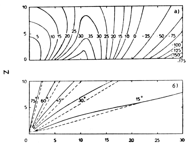
Figure 1: Top: Isolines of $\overline{z_{0}^{2}}$. Bottom: Isolines of the inclination angle, $\alpha$, of the major axis of the velocity ellipsoid with respect to the galactic symmetry plane for $\overline{z_{0}^{2}}=\overline{z_{0}^{2}(R,z)}$ (solid lines) and for $z_{0}=0.5$ kpc (dashed lines).

The averaged parameter $\overline{z_{0}^{2}}$ is not a constant, but a function of coordinates $\overline{z_{0}^{2}}(R,z)$, see Fig. 1 for the M31 model, described in Chapter 18. Mean values of $\overline{z_{0}^{2}}(R,z)$ were calculated using Eq. (65) for the Kuzmin (1956a) model with parameters, given in Table LABEL:Tab18.1.

We saw above that $z_{0}$ gives us the foci of confocal ellipsoids and hyperboloids; in addition, at foci the velocity ellipsoids reduce to spheres. In the present case, the principal velocity-surfaces are no longer ellipsoids and hyperboloids but have a more complicated form. Velocity ellipsoids reduce to spheres at system axis at points $z=\pm z_{0e}$ ($z_{0e}$ are points where $\overline{z_{0}^{2}}(0,z)=z^{2}$). These points can be called effective foci of the composite model.

Formulae derived here solve the problem, established at the beginning of the paper. To our understanding, they allow to calculate a more realistic hydrodynamical model of a galaxy, compared to previous ones. But of course, our method is also only a preliminary one. Further development of the construction of hydrodynamical models of stellar systems is difficult without further development of the theory of the third integral as a quasi-integral, together with the theory of irregular forces in elliptical galaxies. And at last, we would like to call attention to the paramount importance to solve these problems.

March 1969

Chapter 13 Virial theorem and its application to the determination of masses of stellar systems

In the determination of masses of stellar systems and their subsystems, the virial theorem can be used if the system or subsystem is sufficiently isolated. Galaxies consist of a number of populations with mutual influence. An exception is the nucleus of a galaxy which is relatively isolated. Chapter 12 of the Thesis discussed general properties of the virial theorem. Here we consider one special case – the application of the virial theorem to find the mass of the nucleus of M31, as done by Einasto & Rümmel (1970c).

The nucleus of a galaxy can be considered in a good approximation to be an isolated dynamical system. In this case we may apply the tensor virial theorem (Kuzmin 1963b). Assuming a rigid body rotation and ellipsoidal shape for the nucleus we have

$$\overline{\sigma_{R}^{2}}+\frac{1}{3}\omega^{2}\,\overline{a^{2}}=\frac{1}{2}\beta_{R}\,G\,\mathfrak{M}\,a^{-1},$$ (1)

$$\overline{\sigma_{z}^{2}}=\frac{1}{2}\beta_{z}\,G\mathfrak{M}\,a^{-1}.$$ (2)

In these formulae $\omega$ is the constant angular velocity, $G$ the gravitational constant, $\mathfrak{M}\,$ the mass of the nucleus, and

$$\overline{a^{2}}=\frac{1}{\mathfrak{M}\,}\int_{0}^{\infty}\mu(a)a^{2}{\rm d}a\,,$$ (3)

$$a^{-1}=\frac{2}{\mathfrak{M}\,^{2}}\int_{0}^{\mathfrak{M}\,}\frac{M(a){\rm d}M(a)\,}{a},$$ (4)

where

$$\mu(a)=4\pi\epsilon\rho(a)\,a^{2}$$ (5)

is the mass distribution function, and

$$M(a)=\int_{0}^{a}\mu(a){\rm d}a\,$$ (6)

is the integral mass distribution function.

The constants $\beta_{R}$ and $\beta_{z}$ depend on the shape of the system. Denoting $e^{2}=1-\epsilon^{2}$ we have

$$\beta_{R}=\frac{1}{2e^{2}}\left[\frac{\arcsin e}{e}-\epsilon\right],$$ (7)

$$\beta_{z}=\frac{\epsilon^{2}}{e^{2}}\left[\frac{1}{\epsilon}-\frac{\arcsin e}{e}\right].$$ (8)

From (1) - (2) we obtain

$$k_{z}=\frac{\sigma_{z}^{2}}{\sigma_{R}^{2}}=\frac{\beta_{z}}{\beta_{R}}\left(1+\frac{\omega^{2}\overline{a^{2}}}{3\overline{\sigma_{R}^{2}}}\right).$$ (9)

As in the nucleus of the Andromeda galaxy $\omega^{2}a^{2}\ll\sigma_{R}^{2}$, the mean axial ratio of the velocity ellipsoid depends sufficiently only on the axial ratio of the system itself. The value of $k_{z}$, found for the nucleus of the galaxy, can be adopted for $k_{z}(0,0)$.

May 1971

Chapter 14 Some families of models of stellar systems

Methods of determining the mass-distribution in oblate stellar systems were summarized by Perek (1962) who presented a classification of models of stellar systems. A reclassification of models has been undertaken by Kutuzov & Einasto (1968). The present paper deals with the methods for determining the mass-distribution, the point of view being different from that of Perek.

As we will see later, almost all expressions proposed earlier for model construction can be interpreted as particular cases of one general law. This enables us to study various models from a single viewpoint.

To select suitable expressions for constructing the models, some conditions are imposed, restricting the choice of model-parameters. Great attention is given to the behaviour of models in their outer region. These aspects were discussed in Chapter 8.

Table 1:

$\alpha$	$n$	$\epsilon$	Case	Remarks	Model
0;1	1	$\epsilon$	$A$	$a,c,d,e$	Schmidt (1956, 1965)
2	1	0	$B$	$c,e$	Schwarzschild (1954)
2	2	$\epsilon$	$A$	$c,e$	Perek (1962)
2	$n$	0	$B$	$+$	Wyse & Mayall (1942)
2	$n$	$\epsilon$	$A$	$+$	Burbidge et al. (1959)

Table 2:

$\beta$	$\nu$	$\epsilon$	Case	Remarks	Model
$>0$	2	1	$A$	$\beta>2.5$	Lohmann (1964),Veltmann (1965)
1	2	$\epsilon$	$B$	$+$	King (1962)
2	1	$\epsilon$	$B$	$d$	Hubble (1930)
2	2	$\epsilon$	$A$	$d$	Kuzmin (1956a)
2	3	1	$A$	$d$	Bottlinger (1933)
2.5	2	1	$A$	$d$	Lohmann (1964)
$\infty$	$\nu$	$\epsilon$	$A$	$+$	Einasto (1965)
$\infty$	2	$\epsilon$	$A$	$+$	Gauss
$\infty$	1	$\epsilon$	$A$	$+$	Expon.
$\infty$	1/4	$\epsilon$	$B$	$+$	de Vaucouleurs (1948)
$<0$	1	1	$A,\leavevmode\nobreak\ B$	$\beta<-1$	Wallenquist (1959)
$<0$	2	$\epsilon$	$A$	$\beta<-1$	Perek (1962)
$-1$	$\nu$	1	$A$	$c,e$	van Wijk (1949)
$-0$	$\infty$	$\epsilon$	$A$	$c,e$	Homogen.

Table 3:

$\alpha$	$\beta$	$\nu$	Remarks	Model
3	$3/\nu$	$\nu$	$d$	Brandt & Scheer (1965)
3	2	2	$a,d$	Parenago (1950)
3	$3/2$	2	$d$	Kuzmin (1956b)
3	1	3	$d$	Bottlinger (1933)
3	$-1$	2	$c,e$	Perek (1962)
2	$-1$	1	$a,c,d,e$	Schmidt (1956)
0	$-1$	3	$a,c,d,e$	Oort (1927)

Usually the distribution of mass only in very oblate systems is considered. In such a case, the mass distribution can be evaluated directly from the rotation data, since the rotation velocity equals the circular one. In the ellipsoidal case, the pressure term (velocity dispersion) cannot be neglected, as stated by Öpik (1922) and later by Oort (1965). In the central parts of oblate stellar systems, the ellipsoidal component, the bulge, is often prevailing, therefore, even in the oblate systems the exact mass-distribution can be found only from a hydrodynamical model, using the data on both rotation and dispersion. Furthermore, independent data on the distribution of luminosity and mass-to-light ratio can also improve the model.

Basic results of the description of some families of models of stellar systems were published by Einasto (1969a). Here we present in a condensed way the main results of this study.

Some quite general families of the descriptive functions can be constructed by means of the function

$$g(a)=g_{0}\,g^{\ast}(\xi),$$ (1)

where $\xi=a/a_{0}$ is dimensionless distance, $a_{0}$ and $g_{0}$ are scale parameters, and

$$g^{\ast}(\xi)=\left\{\begin{array}[]{ll}\xi^{\alpha}\,\prod^{n}_{i=0}(1+\chi_{i}/\beta_{i}\,\xi^{\nu_{i}})^{-\beta_{i}}&\xi\leq\xi_{0},\\ 0,&\xi\geq\xi_{0}.\end{array}\right.$$ (2)

In the last formula, $\xi_{0}$ is the smallest positive root of the equation

$$g^{\ast}(\xi)=0,$$ (3)

and $\alpha,\leavevmode\nobreak\ \chi_{i},\leavevmode\nobreak\ \beta_{i},\leavevmode\nobreak\ \nu_{i}$ are structural parameters.

The expression $g(a)$ can be identified with various descriptive functions:
$A$)                            $g(a)\equiv\mu(a)$;
$B$)                            $g(A)\equiv L(A)$;
$C$)                            $g(R)\equiv F_{R}(R)$;
$D$)                            $g(R)\equiv V_{\theta}(R)$;
$E$)                            $g(R)\equiv\sigma_{R}^{2}(R)$.

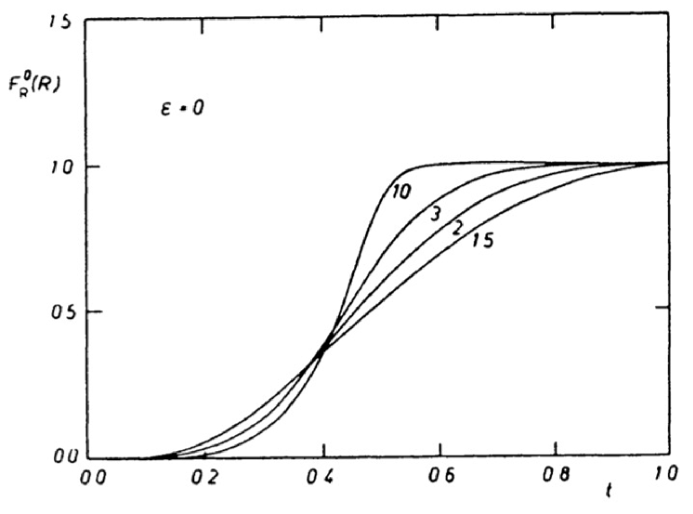
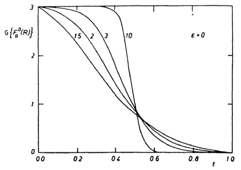
Figure 1: The function $F_{R}^{0}(R)$ and its logarithmic gradient as functions of $t=a/(1+a)$ for the generalised Bottlinger model with parameters $\epsilon=0$ and various $\nu$, shown as index of curves.

The formula (2) is too general and contains too many parameters for practical use. We will consider three families of special models based on the law (2):
a) the polynomial model (cases $A$ and $B$)

$$g^{\ast}(\xi)=\xi^{\alpha}\,\prod^{n}_{i=0}\,(1-\chi_{i}\,\xi),$$ (4)

b) the binomial model (cases $A$ and $B$)

$$g^{\ast}(\xi)=\xi^{\alpha}\,\left(1+1/\beta\,\xi^{\nu}\right)^{-\beta},$$ (5)

c) the generalised Bottlinger model (case $C$)

$$F_{R}^{\ast}(\xi)=\xi^{\alpha}\,\left(1+1/\beta\,\xi^{\nu}\right)^{-\beta}.$$ (6)

In cases $D$ and $E$, the binomial law (5) can also be used.

Most models of galaxies and star clusters proposed earlier are particular cases of models (4) $\dots$ (6). Their review is given in Tables LABEL:Tab13.1 $\dots$ 3. In Tables Remarks letters $a,b,c,d,e$ indicate that the model does not agree with condition $a,b,c,d,e$, discussed in Chapter 8, $+$ indicates that the model agrees with all these conditions. Binomial models with $\beta=\infty$ are generalised exponential models (Einasto 1965), having for spatial density (case A) the form

$$\rho(a)=\rho_{0}\,\exp[-\xi^{1/N}].$$ (7)

The radial attraction function $F_{R}^{0}(R)$ and its logarithmic gradient for the generalised Bottlinger model are shown in Fig. 1, using as argument $t=a/(1+a)$. For the generalised exponential model several descriptive functions are shown in Chapter 15.

May 1968 Revised May 1971

Chapter 15 Polynomial models

The analysis of galactic models has shown that most models were constructed using analytical expressions for descriptive functions of two families, polynomial or binomial models. In this Chapter, I discuss concisely the polynomial models. A more detailed discussion was published by Einasto (1968b, 1969a).

General families of the description functions can be constructed by means of the function

$$g(a)=g_{0}\,g^{\ast}(\xi),$$ (1)

where $\xi=a/a_{0}$ is the dimensionless distance, $a_{0}$ and $g_{0}$ are scaling parameters, and

$$g^{\ast}(\xi)=\left\{\begin{array}[]{rc}\xi^{\alpha}\,\Pi_{i=0}^{n}\,\left(1+{\chi_{i}\over\beta_{i}}\,\xi^{\nu_{i}}\right)^{-\beta_{i}},&\xi\leq\xi^{0},\\ 0,&\xi\geq\xi^{0}.\end{array}\right.$$ (2)

In the last formula, $\xi^{0}$ is the smallest positive root of the equation $g^{\ast}(\xi)=0$, and $\alpha,\leavevmode\nobreak\ \chi_{i},\leavevmode\nobreak\ \beta_{i},\leavevmode\nobreak\ \nu_{i}$ are structural parameters.

Eq. (2) is too general and contains too many parameters for practical use. The polynomial model is defined as

$$g^{\ast}(\xi)=\xi^{\alpha}\,\Pi_{i=0}^{n}\,(1-\chi_{i}\,\xi),$$ (3)

The polynomial model with parameters $\alpha=0,\leavevmode\nobreak\ 1$ and $n=1$ was used in models of the Galaxy by Schmidt (1956, 1965). These models are in conflict with our conditions of physical correctness a), c) and d), discussed in Chapter 8. Wyse & Mayall (1942) used this profile to describe the projected density distribution of M31. The polynomial profile was also used by Burbidge et al. (1959, 1960) in their series of studies of the rotation and mass distribution of galaxies. In the latter cases, most conditions of physical correctness were fulfilled, however, the density function has a break at $\xi^{0}$.

April 1967

Chapter 16 Binomial models

Binomial models were discussed in detail by Einasto (1968c, 1969a), and formed the basis of Chapter 15 of the original Thesis. Here I give a short summary, concentrating on the case of the generalised exponential function.

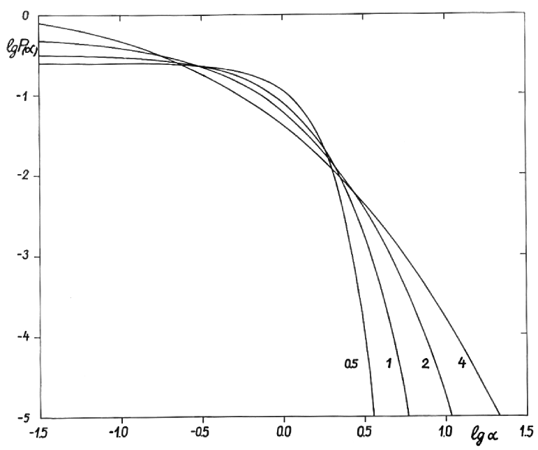
Figure 1: Distribution of the projected density $P(\alpha)$ for the generalised exponential model. Parameter $N$ is shown as an index of curves.

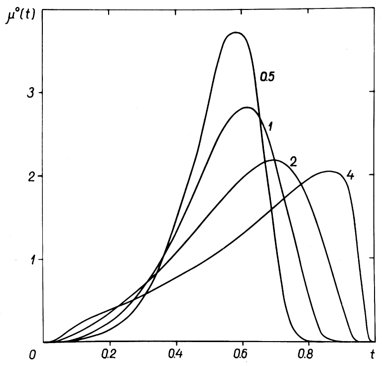
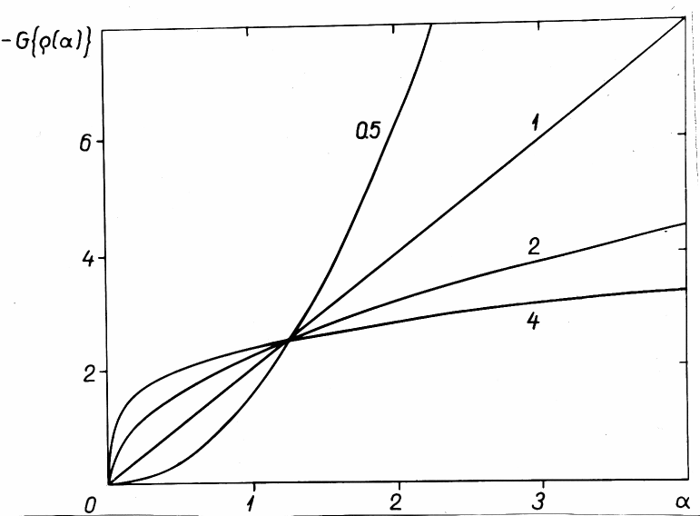
Figure 2: Left: Mass function $\mu^{\circ}(t)$ of generalised exponential model. The shape parameter $N$ is shown. Right: The logarithmic density gradient $G\{\rho(\alpha)\}$ of the generalised exponential model.

Binomial models are defined by the description function

$$g^{\ast}(\xi)=\xi^{\alpha}\,\left(1+1/\beta\,\xi^{\nu}\right)^{-\beta},$$ (1)

where $\xi=a/a_{0}$ is the dimensionless distance, and $\beta$ and $\nu$ are structure parameters. If $\beta\rightarrow\infty$, then the binomial model reduces to the generalised exponential model

$$g^{\ast}(\xi)=e^{-\xi^{\nu}}.$$ (2)

Often as the shape parameter, instead of $\nu$ its reciprocal value is used $N=1/\nu$.

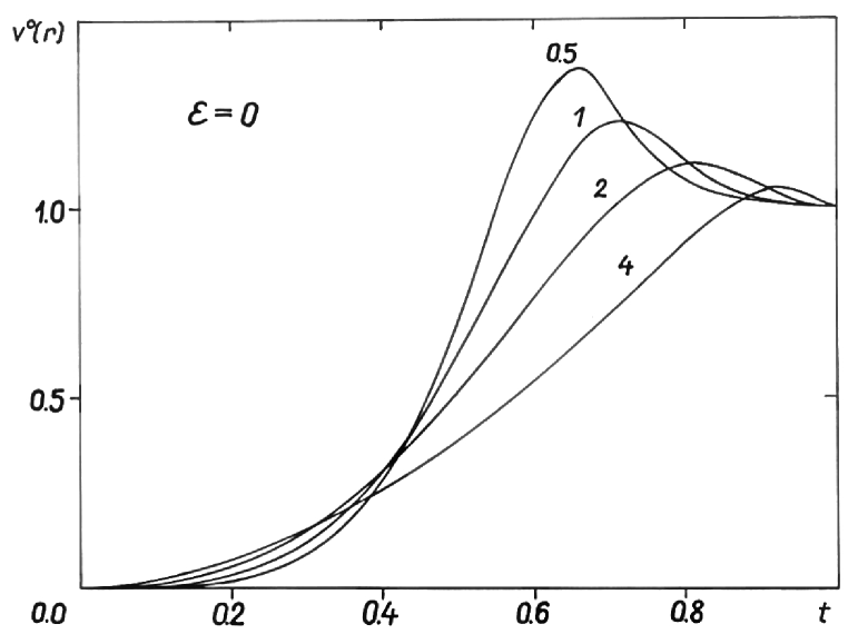
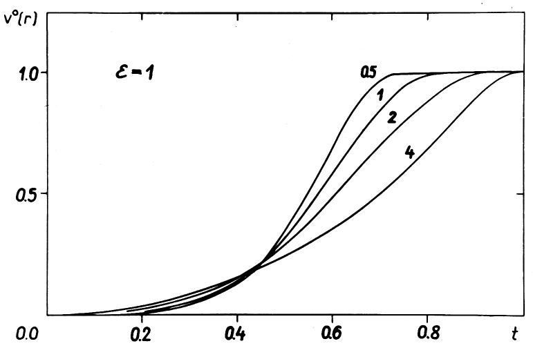
Figure 3: Circular velocity function $v^{\circ}(t)$ of the generalised exponential model for two values of the axial ratio $\epsilon$. The shape parameter $N$ is shown.

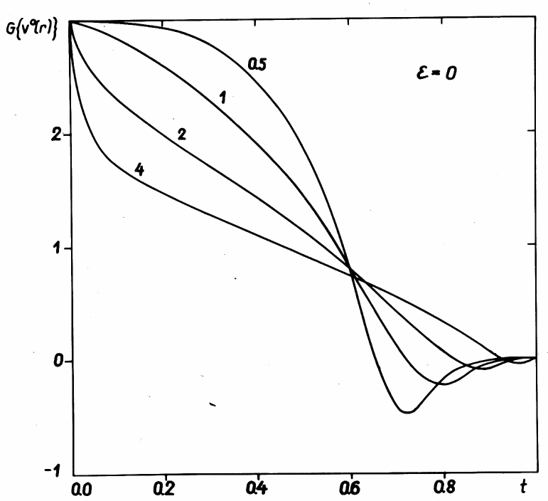
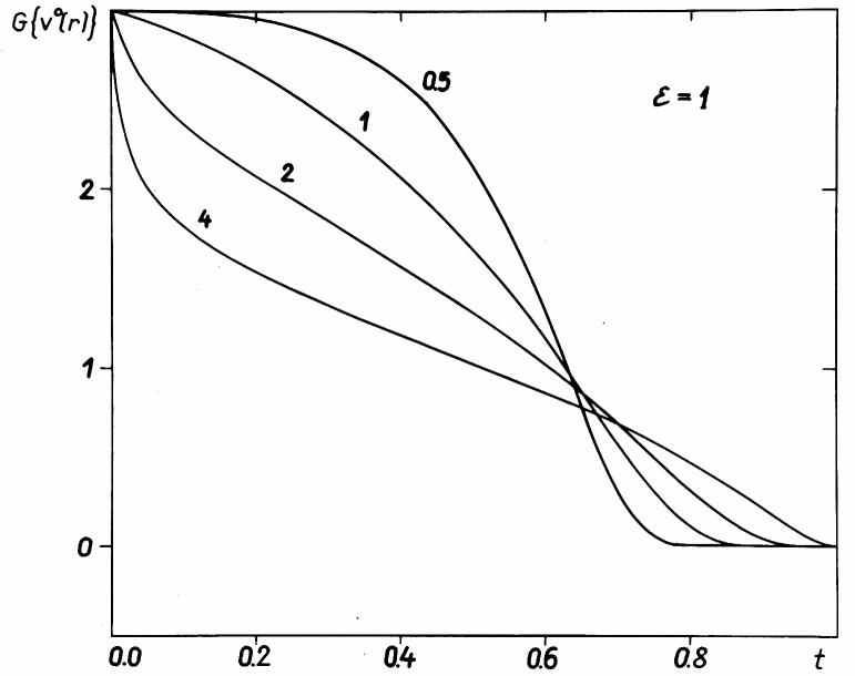
Figure 4: Logarithmic gradient of the velocity $G\{v^{\circ}(t)\}$ of the generalised exponential model for two values of the axial ratio $\epsilon$. The shape parameter $N$ is shown.

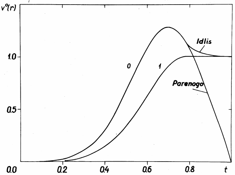
Figure 5: Circular velocity function $v^{\circ}(\alpha)$ for Parenago and Idlis models. The axial ratio $\epsilon$ is shown.

Cases $\nu=2$ and $\nu=1$ are ordinary Gaussian and exponential models. The case $\nu=1/4$, when applied to projected density, is the de Vaucouleurs (1948) profile for elliptical galaxies. It can be used also for the spatial density, as done by Einasto (1965, 1969b).

In the following Figures, several descriptive functions of the generalised exponential function are given. As parameters we use $N=1/\nu$, $\alpha=a/a_{0}$ and $t=\alpha/(1+\alpha)$. Fig. 1 shows the projected density, Fig. 2 left panel gives the relative mass function $\mu^{\circ}(t)=\frac{1}{\mu_{0}}\mu(\alpha)\,(1+\alpha)^{2}$, where $\mu_{0}$ is a normalising constant. Fig. 2 right panel shows the logarithmic density gradient $G\{\rho(\alpha)\}$. Fig. 3 shows the circular velocity function

$$v^{0}(a)=\frac{a}{G\mathfrak{M}\,}\,V^{2}(a),$$ (3)

where $V$ is the circular velocity, $G$ is the gravitation constant, and $\mathfrak{M}\,$ is the mass of the system. The circular velocity of a point mass $\mathfrak{M}\,$ is $V^{2}(a)=\frac{G\mathfrak{M}\,}{a}$, thus the circular velocity function is the relation of squares of circular velocities of the model and the point-mass of the same mass. This definition of the circular velocity function was suggested by Perek (1962). Next, in Fig 4 we give the logarithmic gradient of the velocity function, $G\{v^{\circ}(t)\}$. Finally, in Fig. 5 we show circular velocity functions of models by Parenago (1950) and Idlis (1956).

September 1967

Revised September 1971

Chapter 17 Hydrodynamical models on the basis of the modified exponential function

In Chapters 5 and 7, I described methods to calculate spatial and kinematical models of galaxies, using our own Galaxy as an example. In this Chapter, I shortly discuss some additional aspects of constructing hydrodynamical models on the basis of the modified exponential function.

The set of descriptive functions is fully determined if one dynamical function is given. Theoretically, it is not important which function is given initially. The remaining functions can be calculated by means of the formulae given in Chapters 5 and 7. But from the practical point of view, it is convenient to start from the luminosity distribution function and from the data on the mass-to-light ratio.

The block diagram of the determination of a model of a stellar system from observations is given in Fig. 1, taken from Einasto (1969a). The observed functions and parameters are shown as circles, the calculated and preliminary adopted quantities are presented by rectangular boxes. Three cases are considered:
a) simple (one component) model of an elliptical galaxy (classical method),
b) simple model of an oblate galaxy (classical method),
c) composed hydrodynamical model of a galaxy (new method).

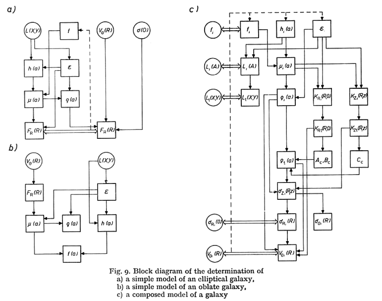
Figure 1: Block diagram of the determination of a) a simple model of an elliptical galaxy, b) a simple model of an oblate galaxy, c) a composed model of a galaxy.

In the first case, the flattening parameter $\epsilon$ and the mass-to-light ratio $f$ is usually assumed to be constant. From the observed projected distribution of luminosity $L(X,Y)$, the corresponding spatial distribution $\mu(a)$ can be found by solving the integral equation

$$L(A)={1\over 2\pi\,E}\int_{A}^{\infty}{\mu(a){\rm d}a\,\over f\,a\sqrt{a^{2}-A^{2}}},$$ (1)

where $a$ and $A$ are major semiaxes of equidensity ellipsoids and projected equidensity ellipsoids, respectively, $L(A)$ is the projected luminosity density, $f$ is the mass-to-light ratio, $\mu(a)=f\,h(a)$ is the mass function, and $h(a)$ the luminosity function. If $f=const$, the mass distribution $\mu(a)$ is similar to the luminosity distribution $h(a)$, and the radial acceleration function

$$F_{R}(R)=\frac{V_{c}^{2}R}{G}=\int_{0}^{R}{\mu(a){\rm d}a\,\over\sqrt{1-(\epsilon\,a/R)^{2}}}$$ (2)

can be found. Here $V_{c}$ is the circular velocity, and $G$ is the gravitational constant. The $F_{R}(R)$ function can be found independently from the kinematical data, using the hydrodynamical equation

$$V_{\theta}^{2}-p\,\sigma_{R}^{2}=V_{c}^{2},$$ (3)

where $V_{\theta}$ is the rotation velocity of a galactic subsystem, $\sigma_{R}$ is the velocity dispersion in $R$ direction of the subsystem, and $p$ is a parameter, depending on the density gradient and the shape of the velocity ellipsoid, see Eqs. (3) and (4). The comparison of the results for $F_{R}(R)$ gives the possibility to determine $f$ and to check the initial assumptions $\epsilon=const$, and $f=const$ (feedback coupling).

In the second case, the usual assumption is $\sigma_{R}\ll V_{\theta}$; from Eqs. (3) and (3) we see that then $V_{\theta}\approx V_{c}$. The mass distribution function, $\mu(a)$, and the luminosity distribution function, $h(a)$, can be determined independently from the integral equations (2) and (4) respectively. The mass-to-light ratio $f$ is to be considered as a function of the distance from the centre of the system.

Observations indicate that the axial ratio of isophotes $E$ of elliptical and spiral galaxies is not constant. Therefore, the assumption $\epsilon=const$ is justified only as the first rough approximation. To obtain a better agreement with observations, $\epsilon$ is to be considered as a variable, as it was taken by Perek (1962), Sizikov (1968) and Kutuzov (1968). In this case, the block diagram of the model determination will not change, but formulae should be replaced by more complicated ones.

The variation of $E$ and $\epsilon$ is caused mainly by the presence of various subsystems, having different flattening $\epsilon$, and different mass and luminosity distribution. Therefore, the structure of a stellar system can be more precisely described by a composed model. The determination of a composed hydrodynamical model of a galaxy (case c in Fig. 1) differs from the determination of a simple classical model in many respects.

As the distribution of luminosity of individual components $L_{i}(X,Y)$ of the galaxy is only partially known, it is difficult to start the model determination from these functions as in previous cases. It would be better to calculate first the normalised descriptive functions, $h^{0}(a)$, $L^{0}(A)$, $F^{0}_{R}(R)$ and $F^{0}_{\theta}(R)$, for a set of concentration and flattening parameters. The construction of the model reduces in this case to the determination of parameters of the galaxy components. For this purpose, both graphical and numerical methods can be used, as done by Einasto (1968d, 1969b).

The evaluation of $z$-velocity dispersion from the vertical acceleration can be made by iterations, as stated by Innanen & Kellett (1968). In the first step, the term with $p$ in formula (3) may be neglected. From the approximate run of velocity dispersions, the correction terms can be calculated. The dispersions $\sigma_{R},\leavevmode\nobreak\ \sigma_{\theta}$, and the centroid velocity $V_{\theta}$ are to be found from $\sigma_{z}$ by using the formulae (3), and

$$\frac{1}{\sigma_{z}^{2}}=\frac{1}{\sigma_{\theta}^{2}}+\frac{1}{\sigma_{R}^{2}},$$ (4)

found from the theory of irregular forces for the case $z\ll R$ (Kuzmin 1961). Furthermore, the Lindblad formula

$$k_{\theta}=\frac{-B}{A-B}=\frac{1}{2}[1+G\{V_{\theta}(R)\}]$$ (5)

can be used, where $G\{V_{\theta}(R)\}$ is the radial logarithmic gradient of the rotation velocity $V_{\theta}(R)$.

A comparison of the calculated descriptive functions with the observed ones (see case c in Fig. 1) gives the possibility to improve the initial descriptive parameters. So, the model will be determined by a trial-and-error procedure. To facilitate the determination of models of stellar systems, we are computing the main dynamical descriptive functions for the exponential model with $\nu$ and $\epsilon$ as parameters. This work is in good progress now (Einasto & Einasto 1972b). Results are published for our Galaxy by Einasto (1970a) and are presented in Chapter 7, and for the Andromeda galaxy M31 by Einasto (1969b, 1970c), Einasto & Rümmel (1970b, 1972) and are discussed in Chapters 18 and 20.

May 1971

Part 3 Spatial and kinematical structure of the Andromeda galaxy

Chapter 18 Model of mass distribution of M31: Preliminary version

On the basis of the published photographic and photoelectric data on the luminosity distribution along the major and minor axis of the galaxy M31, the model of the latter was elaborated (Einasto 1969b), which is the topic of this Chapter. The model consists of four components: the nucleus, bulge, disc, and flat component. The masses of components were derived from the velocity data, collected from optical and radio sources. The velocity dispersion and the mass-to-light ratio, spectroscopically obtained for the centre of M31, were also used.

It was found that the circular velocity curve has a maximum $V_{c}=380$ km/sec at the distance of 4’ from the centre. The rotational velocity of the spheroidal component (the bulge) equals only 125 km/sec in this region. The great difference between the circular and rotational velocities can be explained by the great velocity dispersion and radial density gradient of the spheroidal component. The dynamical mass-to-light ratio 17.3 is in good agreement with the spectroscopical one, 16.7.

For the mass of the galaxy M31, a value of $200\times 10^{9}$ solar masses is found. Considerably greater values obtained by other authors (see Table LABEL:Tab17.3) are biased by neglecting the fact that the galaxies are of finite sizes.

In the motion of interstellar hydrogen, local deviations from the circular motion occur.

1 Introduction

The study of the structure of the large Andromeda galaxy M31 is of interest primarily because it is the closest outer spiral galaxy to us. This allows us to find out its structure in details that are not visible or difficult to study in other, more distant galaxies. In addition, it is well known that the M31 galaxy is very similar in structure to our Galaxy. Due to this circumstance, the study of M31 galaxy complements the study of our Galaxy and vice versa.

Among the results obtained in the study of the general structure of the M31 galaxy there are the following two contradictory conclusions.

1. Estimates of the mass of the system, despite a very precisely defined rotation curve, are very different, ranging from 200 to 600 billion solar masses.

2. According to the dynamical definition, the ratio of mass to luminosity $f$ at the centre of the system is very small, while on the periphery it approaches infinity (see Fig. 6). On the other hand, according to the spectral definition of the composition of the M31 core, the central value of $f$ is approximately equal to its mean value, i.e. the value of $f$ must be approximately constant.

In the present series of articles, a model of the M31 galaxy will be constructed, and an attempt will be made to clarify the reasons for the above contradictions. It is assumed that the M31 galaxy consists of four main components: the nucleus, bulge, disc, and flat component. In the course of the work, it turned out that the model can be constructed by successive approximations. Therefore, this first article of the series describes a preliminary model of the system. In the future, the model will be refined and detailed.

2 Description functions and the equations of the relationship between them

From observations it is possible to determine the following functions or their partial values: the projected luminosity density $L_{S}(X,Y)$ in the photometric system $S$ ($X$ and $Y$ are rectangular visible coordinates expressed in angular units, with the $X$ axis directed along the visible major axis of the galaxy, and $Y$ along the minor axis); the rotation speed of some subsystems $V_{\theta}$; the stellar velocities dispersion $\sigma$, and the stellar composition (for the galactic nucleus). It is also possible to study the distribution and physical properties of individual bright stars.

In order to model the galaxy, it is necessary to introduce simplifying assumptions. In this series of works, it is assumed that the M31 galaxy can be divided into a finite number of physically homogeneous components, whose equidensity surfaces are similar coaxial ellipsoids of rotation. The ratio of semiaxes of ellipsoids of different components $\epsilon$ can be different, the density changes smoothly.

Since the main description functions are additive (except for rotation velocity $V_{\theta}$ and velocity dispersion $\sigma$), for simplicity we will write their connection equations not for the total values but for the individual components.

Let $\rho(x,y,z)$ be the spatial mass density of the component, and $l_{S}(x,y,z)$ — the spatial luminosity density in the photometric system $S$ ($x,\leavevmode\nobreak\ y,\leavevmode\nobreak\ z$ are rectangular galactocentric coordinates, the $z$ axis is directed along the system axis). With the above assumptions

$$\rho(x,y,z)=\rho(a)=f_{S}\,l_{S}(a),$$ (1)

where

$$a^{2}=x^{2}+y^{2}+\epsilon^{-2}z^{2},$$ (2)

and $f_{S}$ is the mass-to-light ratio of the component. The mass and luminosity densities are related as (Einasto 1968a)

$$\mu(a)=4\pi\epsilon\,a^{2}\rho(a)$$ (3)

and

$$h_{S}(a)=4\pi\epsilon\,a^{2}\,l_{S}(a).$$ (4)

The projected density of components is expressed (Einasto 1968a)

$$L_{S}(A)=\frac{1}{2\pi\,E}\int_{A}^{\infty}\,{h_{S}(a){\rm d}a\,\over a\sqrt{a^{2}-A^{2}}},$$ (5)

where

$$A^{2}=X^{2}+E^{-2}Y^{2},$$ (6)

$$E^{2}=\cos^{2}i+\epsilon^{2}\,\sin^{2}i,$$ (7)

where $i$ is the angle between the symmetry axis of the system and the line of sight.

The rotation velocity of the component and the circular velocity of the whole system, $V$, are related as (Kuzmin 1962) (see also Chapters 7 and 11):

$$V_{\theta}^{2}-p\,\sigma_{R}^{2}=V^{2},$$ (8)

where $\sigma_{R}$ is the velocity dispersion of the component in the radial direction ($R^{2}=x^{2}+y^{2}$), and the dimensionless parameter $p$ is expressed as

$$p=\left(1-\frac{\sigma_{\theta}^{2}}{\sigma_{R}^{2}}\right)+R\,\left(1-\frac{\sigma_{z}^{2}}{\sigma_{R}^{2}}\right)\frac{\partial\alpha}{\partial z}+G\{\rho(R)\}+G\{\sigma_{R}^{2}(R)\},$$ (9)

where $\alpha$ is the inclination angle of the vertex in respect to the plane of the system (outside the symmetry plane $\alpha\neq 0$).

In the last equation we used for the logarithmic gradient $G$ the expression

$$G\{f(R)\}=\frac{\partial\,\ln f(R)}{\partial\,\ln R}.$$ (10)

The expression for $p$ in the form (9) is inconvenient for practical applications, since neither the ratio of velocity dispersion nor the gradient of the angle $\alpha$ can be directly found from observations. When transforming the expression $p$, we will use the relations found by (Kuzmin 1952b, 1961)

$$R\frac{\partial\alpha}{\partial z}=-\frac{1}{4}\,G\{\rho_{t}(R)\},$$ (11)

and

$$\frac{1}{\sigma_{z}^{2}}=\frac{1}{\sigma_{\theta}^{2}}+\frac{1}{\sigma_{R}^{2}},$$ (12)

and the Lindblad equation

$$\frac{\sigma_{\theta}^{2}}{\sigma_{R}^{2}}=\frac{-B}{A-B}.$$ (13)

Formulas (11) - (13) are derived for flat subsystems. However, the calculations show that in the vicinity of the Sun these formulas can be applied to less flattened subsystems as well. Therefore, we can assume that the use of these formulas in constructing the model of the M31 galaxy is not associated with large errors.

In the Lindblad formula for planar subsystems, the Oort parameters $A$ and $B$ can be expressed through the circular velocity $\omega(R)=V_{\theta}/R$ and the logarithmic gradient of the circular velocity function $G\{v(R)\}$, with the circular velocity function defined by the formula (Einasto 1968a) (see Eq. 3)

$$v(R)=\frac{V^{2}\,R}{G\,\mathfrak{M}\,},$$ (14)

where $G$ is the gravitation constant, and $\mathfrak{M}\,$ the mass of the system. We get

$$A(R)=\omega(R)=\frac{3-G\{v(R)\}}{4}$$ (15)

and

$$B(R)=-\omega(R)\frac{1+G\{v(R)\}}{4},$$ (16)

and using Eq. (12) and (13)

$$k_{\theta}=\frac{\sigma_{\theta}^{2}}{\sigma_{R}^{2}}=\frac{3-G\{v(R)\}}{4}$$ (17)

$$k_{z}=\frac{\sigma_{z}^{2}}{\sigma_{R}^{2}}=\frac{1+G\{v(R)\}}{5+G\{v(R)\}}.$$ (18)

After these substitutions we get for $p$ the expression

$$p={3-G\{v\}\over 4}-{G\{\rho_{t}\}\over 5+G\{v\}}+G\{\rho\}+G\{\sigma_{R}^{2}\}.$$ (19)

The same expression is also valid for spherical subsystems if we suppose that $V_{\theta}\approx V$. In a more exact consideration, in the expression for $p$ the circular velocity should be replaced by the rotational velocity of the subsystem $V_{\theta}$.

The circular velocity $V(R)$ is related to the mass function by the equation (Einasto 1968a)

$$V^{2}(R)=\frac{G}{R}\int_{0}^{R}\,{\mu(a){\rm d}a\,\over\sqrt{1-(ea/R)^{2}}},$$ (20)

where $G$ is the gravitation constant and $e^{2}-1-\epsilon^{2}$.

Finally, we also use the Poisson equation in terms of Oort-Kuzmin parameters (Kuzmin 1952b)

$$4\pi\,G\rho_{t}=C^{2}-2\,(A^{2}-B^{2}),$$ (21)

where $C$ is the Kuzmin parameter. For flat populations, it can be found from the relation

$$C=\sigma_{z}/\zeta,$$ (22)

where $\sigma_{z}$ and $\zeta$ are dispersions of $z$-velocities and $z$-coordinates of stars, respectively.

3 Choosing the form of the main description function

A model of mass and luminosity distribution of the galaxy is completely defined if the luminosity distribution of its subsystems is known, as well as the mass-to-light ratio of subsystems. Using Eqs. (1), (4) and (5) the mass distribution of the system can be found, and by Eqs. (3) and (20) the circular velocity $V$ can be calculated. Due to the proportionality of $\rho$ and $l_{S}$, we shall write formulas only for one of them, $\rho$.

To build a hydrodynamical model, in addition to the mass distribution function and related functions, we must also know the rotation velocity and velocity dispersion of subsystems. Then by Eqs. (8), (12) and (13) we can calculate other hydrodynamical functions of interest. The Poisson equation (21) allows us to check the obtained results.

To summarise, the hydrodynamical model is completely defined by specifying functions $\rho(a)$, $V_{\theta}(R)$, and parameters $\epsilon$ and $f$ of all components of the galaxy.

The representativeness of the model depends essentially on the choice of the type of these basic description functions. It is natural to demand that description functions have no sharp jumps and kinks, that $\rho(a)\geq 0$ and $\sigma_{R}^{2}(R)\geq 0$. Since real stellar systems have finite sizes (due to the perturbing action of neighbouring systems), it is desirable to choose for $\rho(a)$ an expression that decreases fast enough with increasing $a$. On the other hand, $\rho(a)$ should not decrease too fast, since in this case the circular motion is unstable.

Taking into account all these considerations, we chose for $\rho(a)$ a generalised exponential function (Einasto 1965, 1968c)

$$\rho(a)=\rho_{0}\,\exp\left[-\left(\frac{a}{a_{0}k}\right)^{\nu}\right],$$ (23)

where $\rho_{0}$ (central density) and $a_{0}$ (effective radius) are scale parameters, $k$ is a dimensionless normalising parameter (see Einasto (1968c), and $\nu$ is a structural parameter of the model, determining the concentration of mass to the centre. Structural parameters of the model also include $\epsilon$, which determines the thickness of the model.

In the case of the flat component, the simple ellipsoidal model represents the density distribution poorly. It is known that in the central regions of galaxies there are no representatives of flat subsystems — emission nebulae and stellar associations (Arp 1964b; van den Bergh 1964). To take this circumstance into account in our model, we used an artificial method: the density of the component was calculated as the difference of two ellipsoidal models:

$$\rho(a)=\rho_{+}(a/a_{0},\rho_{0},\nu,\epsilon)-\rho_{-}(a/(a_{0}\kappa),\rho_{0},\nu,\kappa\epsilon),$$ (24)

where $\kappa>1$. With such $\rho(a)$ automatically $\rho_{R=0}(z)=0$. With a suitable choice of $\rho(a)$, the conditions $\rho(a)\geq 0$ and $\partial\rho/\partial z^{2}<0$ at $z\neq 0$ are still satisfied.

In the framework of the preliminary model of the M31 galaxy, it is sufficient to fix hydrodynamical functions only for the spherical component, the core. In this case, the rotation speed of the component can be represented by the formula (Brandt & Scheer 1965)

$$V_{\theta}=V_{0}{R\over[1+(R/R_{0})^{n}]^{3/2n}}.$$ (25)

4 Observational data

1. The photometric data on the brightness distribution along the major and minor axes of the M31 galaxy were collected from all available sources. Only the data that could be reduced to the UBV system were used (see de Vaucouleurs (1958) and Kinman (1965)). In order to build a composite model, it would be desirable to have photometric data in different colours. However, a sufficiently wide brightness interval is covered only by the data in blue rays, so we had to limit ourselves to a single photometric system B. We used from photographic observations results by Redman & Shirley (1937), Fricke (1954), Johnson (1961), Richter & Högner (1963), and from photoelectric observations those by Thiessen (1955) and de Vaucouleurs (1958).

To form a summary curve of the brightness distribution of the M31 galaxy, the data for the NE and SW halves of the major axis, as well as for the NW and SE halves of the minor axis were combined, and the corresponding brightnesses were averaged. The agreement between the NE and SW half-axes is good everywhere. The agreement between the NW and SE hemispheres is less good, especially in the strong absorption region of the NW hemisphere at 4.5 to 17’ from the centre. In the preliminary M31 model, this region was excluded. Similarly, the general uniform absorption was not taken into account, neither in our Galaxy nor in the M31 galaxy.

The derived summary values of the projected luminosity along the major axis are indicated by dots in Fig. 1. Fig. 2 shows the change of the ratio of the semi-axes of the isophotes $E$. As an argument we use $R^{1/3}$, and respective angular distance from the centre of the system along the major axis, expressed in arc minutes.

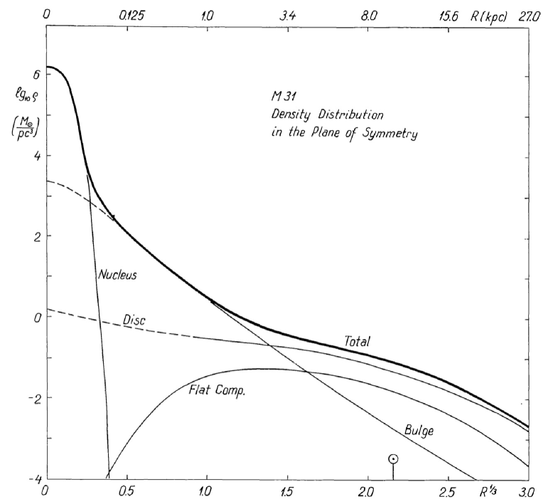
Figure 1: Luminosity distribution along the major axis of M31 (Einasto & Rümmel 1970c).

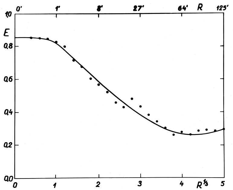
Figure 2: Distribution of the axial ratio $\epsilon$.

2. The rotational velocity was determined from optical (Babcock (1939), Wyse & Mayall (1942), Mayall (1951) and Lallemand et al. (1960)) and radio data (van de Hulst et al. (1957), Burke et al. (1963), Argyle (1965), Gottesman et al. (1966) and Roberts (1966)). In the central region ($R\leq 10^{\prime}$) only optical data were used, because the velocity changes rapidly and radio observations have too low resolution. In the distance range $10^{\prime}<R\leq 50^{\prime}$ both optical and radio data were used, in the region $R>50^{\prime}$ only the radio data were used as more accurate. The mutual consistency of the radio data obtained by different authors is very good. For the velocity of the galaxy centroid a value $-300$ km/s was chosen. With this choice the regions of maximum velocity on both sides of the centre agree best. The observed rotational velocities are depicted in Fig. 3 by dots.

3. The distance of the M31 galaxy was assumed to be $d=692$ kpc according to the true distance modulus $(m-M)_{0}=24.2$ (Baade & Swope 1963).

4. The inclination of the galaxy was determined according to the apparent ratio of semi-axes isophotes $E$, and from the apparent distribution of emission nebulae (Arp 1964a). The found value, $i=77.^{\circ}2$, agrees well with the Baade & Swope (1963) estimate, $i=77.^{\circ}3$, and with the result by (Arp 1964a), $74^{\circ}<i<79^{\circ}$).

5. Additional data can be obtained for the central, brightest regions of the system. The Minkowski velocity dispersion of the core stars is $\sigma_{R}=225$  k/sec (Lohmann 1964), and the Spinrad (1966) mass-to-light ratio $f=16.7$.

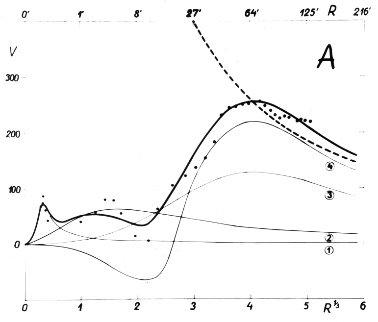
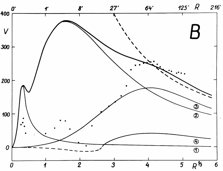
Figure 3: Distribution of the rotation velocity. Masses of components are taken for variants A and B, see Table LABEL:Tab17.1. Thin curves show contributions of components, the bold solid curve shows the rotation curve of the whole model. The dashed curve gives the Keplerian rotation curve, corresponding to a point source with a mass, equal to the mass of the model

5 Model construction

The construction of a model with a fixed analytical form of the main description functions is reduced to the determination of parameters of these functions. In this case we need to find the following parameters for all four components of the model:
a) scale parameters $l_{0}$ and $a_{0}$;
b) structural parameters $\nu$ and $\epsilon$;
c) dynamical parameter $f$.

For the spherical component it is also necessary to know the parameters of the rotation law (25).

The analysis of observational data showed that both scale and structural parameters of the components cannot be found with sufficient accuracy from the rotation velocity. In addition to the mass distribution, the relative motions of the stars also influence the rotation velocity. de Vaucouleurs (1958) showed that model parameters can be found quite successfully from the photometric data.

Using these considerations we determined parameters $l_{0},\leavevmode\nobreak\ a_{0},\leavevmode\nobreak\ \nu_{0}$ and $\epsilon$ from the photometric material. The practical procedure was reduced to the following.

As the first step, we calculated for a number of values of the parameter $\nu$ the normalised projected density function $L^{0}(\alpha)$, and the velocity function $v^{0}(\alpha)$, where $\alpha$ is the dimensionless normalised distance (semi-major axis). The normalisation was performed so that moments of order $-1$ and 0 of the mass function $\mu^{0}(a)$ were equal to one (see Einasto (1965)).

The calculated functions $L^{0}(\alpha)$ were plotted in the logarithmic scale $\log\,L^{0}(\log\,\alpha)$. Similar plots were made for the observed projected luminosity M31 on the major and minor axes. Since the scale transformations (offsets on the logarithmic scale) do not change the shape of the $\log\,L^{0}(\log\,\alpha)$ curve, the parameter $\nu$ can be found by the comparison of the model curve with the observed one. The parameter of apparent flatness $E$ can be found from the comparison of density distributions on minor and major axes. The true axial ratio of semiaxis $\epsilon$ can be found from Eq. (7).

The practical difficulty in the calculation of the model is due to the need to find parameters of all four components simultaneously. However, density distributions of components are very different, see Fig. 1. After several trials optimal parameters of components were found.

This procedure cannot be applied to find the $\epsilon$ parameter for the flat component. In this case $\epsilon$ was chosen in such a way that the effective half-thickness of the components

$$z_{e}=\frac{1}{2}\,\frac{P(R)}{\rho(R)},$$ (26)

has an acceptable value. Here $P(R)$ is the projected mass density of the system.

Table 1: Parameters of the components of M31

Quantity	Unit	Total	Nucleus	Bulge	Disc	Flat+	Flat$-$
$\epsilon$			0.84	0.57	0.09	0.01	0.02
$\nu$			1	1/4	1	1	1
$k$			0.5	$1.26\times 10^{-4}$	0.5	0.5	0.5
$a_{0}$	kpc		0.025	5	50	40	20
$L$	$10^{9}\,L_{\odot}$	13.13	0.003	4.95	6.46	2.29	$-0.57$
$\mathfrak{M}\,_{A}$	$10^{9}\,\mathfrak{M}\,_{\odot}$	201	0.009	2.4	58	188	$-47$
$\mathfrak{M}\,_{B}$	$10^{9}\,\mathfrak{M}\,_{\odot}$	201	0.05	85.5	111.5	5.73	$-1.43$
$f_{A}$		15.3	2.5	0.5	9	82	82
$f_{B}$		15.3	17.3	17.3	17.3	2.5	2.5

Parameter values for components are given in Table LABEL:Tab17.1 (mass-to-light ratios $f$ are in photometric system B). The model is presented in a graphical way in Figs. 1 and 2. In Fig. 1 thin lines show the contributions of components to the total luminosity (along the long axis), the bold line shows the summed total luminosity. We see that the model represents observations (shown as points) rather well. Differences between the model and observations are due to the fact that populations do not contain information on individual spiral arms but only their mean structure.

Mass-to-light ratios of populations can be derived in two ways: A) using the rotation speed; B) using the spectral information of stellar components from independent sources.

In the first case, it is assumed that the rotation velocity is equal to the circular velocity, $V_{\theta}=V$. In practical use, this means that by a trial-and-error procedure values of $f$ are chosen (at fixed parameter $a_{0}$ values), which yield for the circular velocity values in accordance with the observed rotation velocity. Values of $f$ found in this way are given in Table LABEL:Tab17.1 (variant A), respective rotation curves are shown in Fig 3. As in Fig. 1, thin lines show the contribution of individual components, the bold line is the total calculated rotation curve, and the dots are observations. The dashed line gives the Keplerian rotation curve, corresponding to a point source with a mass, equal to the mass of our model. We see that the theoretical curve represents observations well.

It should be said that the flat component of the model has a toroidal form. Inside the toroid, the attraction vector is directed not towards the centre of the system but towards the nearest side of the toroid. Therefore, in this region the velocity function is negative, and circular motion is impossible (unless there are other components that compensate for the negative region of the velocity function). In Fig. 3 this region of the component contribution to the rotation curve is shown by a dashed line.

In the second version B the parameters were found as follows. For the nucleus of M31 $f$ was obtained by Spinrad (1966) from spectral observations, $f=16.7$. The flat component consists mainly of hydrogen, whose mass according to van de Hulst et al. (1957), Argyle (1965), Gottesman et al. (1966), and Roberts (1966) can be taken as equal to $\mathfrak{M}\,=3.7\times\,10^{9}\leavevmode\nobreak\ M_{\odot}$. The mass of the flat component of stars can be estimated from the integral luminosity of the component, and the initial luminosity and mass function (Salpeter (1955), Sandage (1957a)). As a result, we obtained for the mass of the component $\mathfrak{M}\,=4.3\times\,10^{9}\leavevmode\nobreak\ M_{\odot}$. Since $L=1.72\times 10^{9}L_{\odot}$, we get $f=2.5$. Knowing the luminosity of all components, and $f$ of the nucleus and the flat component, it is not difficult to calculate $f$ of the disc. The result coincides almost exactly with the value of $f$ for the nucleus, found by Spinrad. Therefore, we assumed that all components, except the flat component, have the identical mass-to-light ratio (variant B in Table LABEL:Tab17.1). The corresponding rotation curves are given in Fig. 3.

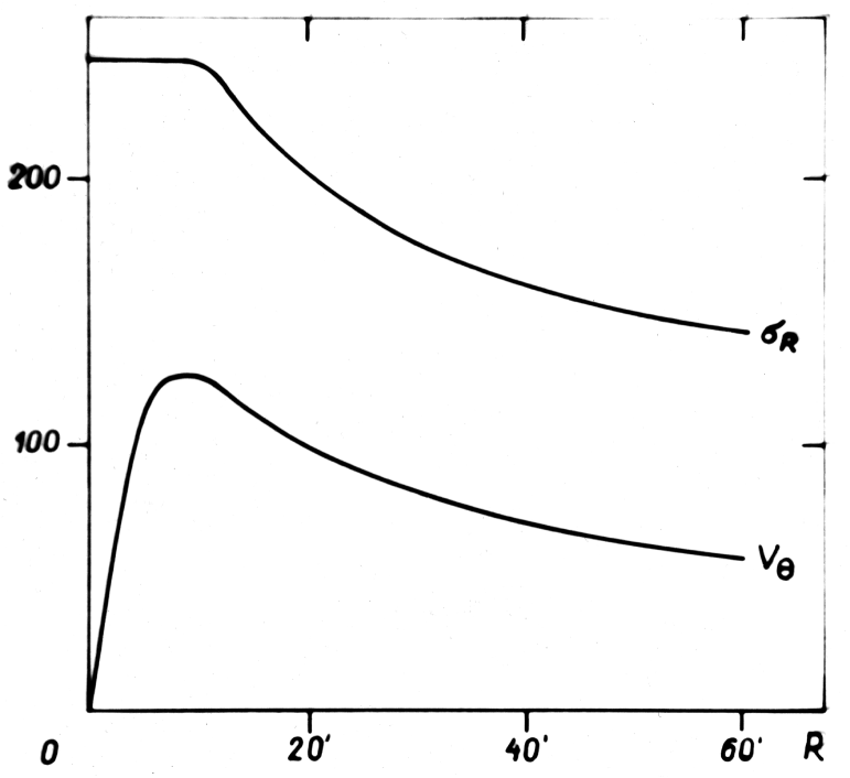
Figure 4: Rotation velocity $V_{\theta}$ and velocity dispersion $\sigma_{R}$ for the spherical subsystem.

In this variant, in the region $R<50^{\prime}$, the circular velocity is noticeably greater than the rotation speed, and reaches at $R=4^{\prime}$ a maximum value, $V=380$  km/sec. The observed rotational velocity at $R=4^{\prime}$ is only $V_{\theta}=80$ km/sec. Thus, a question arises, can the velocity centroid shift reach such a large value, $\Delta\,V=V-V_{\theta}=300$ km/sec?

Calculations using formulas (8) and (19) showed that, within the accuracy of the initial data, such a shift can indeed be explained. Fig. 4 shows one possible variant of the rotational velocity $V_{\theta}$, and the velocity dispersion $\sigma$ of the spherical component of M31. For $V_{\theta}$, the profile (25) was taken; $\sigma_{R}$ was determined by Eq. (8). In our calculations, we took into account the fact that the observed $V_{\theta}$ and $\sigma_{R}$ are lower than their actual maximum values. This is caused by the fact that we observe some mean value of the dispersion and velocity (van Houten 1961)

$$V_{\theta}(R)={\int_{-\infty}^{\infty}\,V_{\theta}(R,Z)\,l(R,Z){\rm d}Z\,\over\int_{-\infty}^{\infty}\,l(R,Z){\rm d}Z\,},$$ (27)

where $Z$ is the coordinate along the line of sight. In the region $R<10^{\prime}$, it was also necessary to slightly change the course of the density gradient, which is also quite acceptable within the accuracy of the available data.

Table 2: Description functions of the M31 model

Table 3: Parameters of models of M31

Author	$n$	$d$	$\mathfrak{M}\,$	$\mathfrak{M}\,^{\ast}$
		kpc	$10^{9}\,M_{\odot}$	$10^{9}\,M_{\odot}$
Lohmann (1964)	3/2	460	330	500
Schwarzschild (1954)		460	140	210
Schmidt (1957b)		630	338	370
Takase (1957)		540	200	260
Poveda (1958)		500	200	280
Brandt (1960)	3/2	600	370	430
Brandt & Scheer (1965)	3/2, 3, 10	630	580	640
Gottesman et al. (1966)	3/2	630	480	530
Roberts (1966)	3/2, 3	690	220	220
Einasto (1969b)		690	200	200

Notes: $n=$ is the structural parameter of the generalised Bottlinger model, Eq. (13); $d$ is distance of M31; $\mathfrak{M}\,^{\ast}$ is mass of M31, reduced to distance $d=690$ kpc.

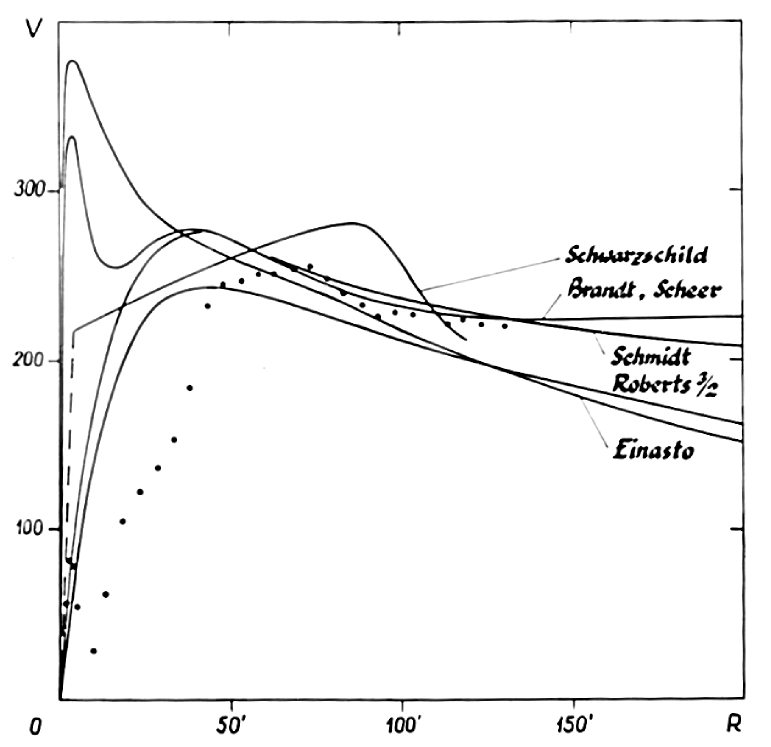
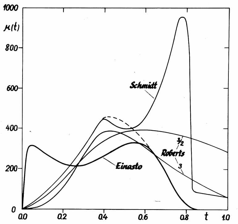
Figure 5: Left. Circular velocity $V(R)$ of models by Schwarzschild (1954), Brandt & Scheer (1965), Schmidt (1957b), Roberts (1966) ($n=3/2$) and Einasto (1969b) (variant B). Right: Mass function $\mu(t)$ for models by Schmidt (1957b), Roberts (1966) ($n=3/2$) and Einasto (1969b) (variant B). Mass is given in units $10^{9}\,\mathfrak{M}\,_{\odot}$. If the Schmidt model is extrapolated according to the dashed line, then its mass is equal to the mass of our model.

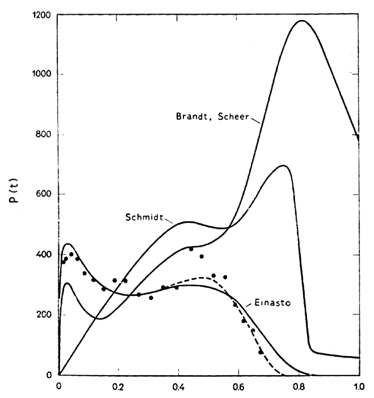
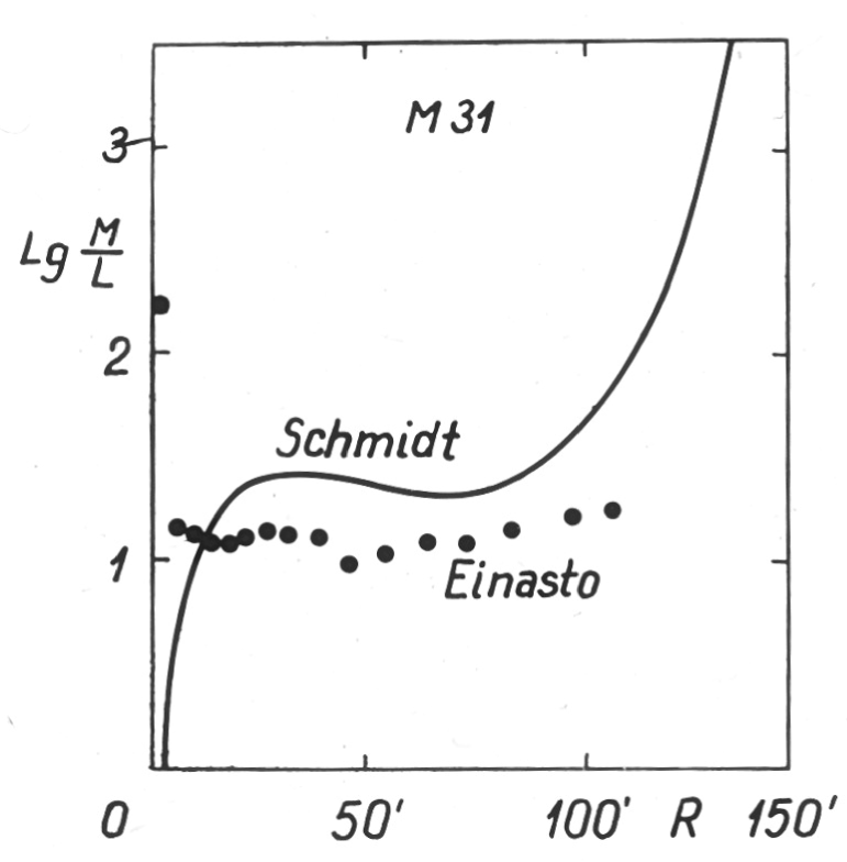
Figure 6: Left. Distribution of the projected density $P(t)$ as function of $t$ for model by Brandt & Scheer (1965), Schmidt (1957b), and Einasto (1969b) (both variants) in units of $10^{9}\,M_{\odot}$. Right: Mass-to-light ratio $f$ of models by Schmidt (1957b) (solid curve) and Einasto (1969b) (dots).

We conclude that the dynamical definition of $f$ agrees well with the spectral definition in the variant B. Calculated values of the description function are shown in Table 2. Here, $V_{k}$ denotes the critical velocity, calculated from the velocity function $v(R)$, using the formula (Einasto 1965)

$$V_{k}^{2}(R)=2\,\int_{R}^{\infty}\,\frac{v(x){\rm d}x\,}{x^{2}}.$$ (28)

In the Table, logarithmic gradients of the density of components $G\{\rho(R)\}$ are also given. In studies of the Galaxy, the gradients $m(R)=-\partial\,\ln\,\rho(R)/\partial\,R$ can be easily calculated by the equation

$$m(R)=-\frac{Mod}{R}\,G\{\rho(R)\}.$$ (29)

From the Table 2 we see that the values of the description functions of the Andromeda galaxy at a distance of 10 kpc from the centre agree very well with the system of local circumsolar parameters in our Galaxy (Einasto & Kutuzov 1964a, b).

6 Analysis of the model

In Table LABEL:Tab17.3 we give main parameters of M31 models, as found by various authors. Here $d$ is the distance of M31, accepted by authors, $\mathfrak{M}\,$ is the mass of M31 according to authors, and $\mathfrak{M}\,^{\ast}$ is the mass, reduced to distance $d=690$ kpc. In left panel of Fig. 5 we show circular velocity $V(R)$ of models by Schwarzschild (1954), Brandt & Scheer (1965), Schmidt (1957b), and Roberts (1966) in comparison with our model. In right panel of Fig. 5 we show the corresponding mass functions

$$\mu_{t}(t)=(1+a)^{2}\,\mu(a)=(1+a)^{2}\,\sum_{k=1}^{n}\,\mu_{k}(a)$$ (30)

and in Fig. 6 the projected on the symmetry plane of the system mass density

$$P_{t}(t)=2\pi\,a\,(1+a)^{2}\,P(a)=2\pi\,a\,(1+a)^{2}\,\sum_{k=1}^{n}\,P_{k}(a).$$ (31)

In these formulas $n$ is the number of components of the model, and we use as argument

$$t=\frac{a}{1+a},$$ (32)

where $a$ is expressed in degrees. This argument is used to represent better distributions on the periphery of the model.

A comparison of the models shows that there are differences in the mass distribution both inside the model and in the peripheral regions of the model. Differences of the first kind change the mass-to-light parameter $f$; total masses of systems, $\mathfrak{M}\,$, do not depend on them much. Differences of the second kind influence both the mass-to-light ratio $f$ and the mass of the system. Since these differences are caused by different reasons, let us consider them separately.

A. The structure of the inner regions of the model is determined to a large extent by the way of treatment — whether the centroid velocity asymmetric shift will be taken into account or not. In most of the works cited above, as well as in our version A, the presence of asymmetric shift was ignored. This way of treatment meets the following objections.

1) The inner regions of the galaxy are dominated by the bulge, whose stars have a large velocity dispersion. This is also confirmed by direct determination of the dispersion. Therefore, in equation (8), the second term on the left is greater than the first one and neglecting it is not justified.

2) The assumption of $V_{\theta}=V$ leads to the conclusion that in central regions of the galaxy the mass-to-light ratio $f$ is small (see Schmidt (1957b) and Figs. 3 variant A, and 6). The study of elliptical galaxies, however, shows that the mass-to-light ratio of stars with enhanced metal content of the population II has a rather large value ($f>10$, see Chapter 22). This is confirmed by direct spectral observations (Spinrad 1966). Therefore, the assumption of $V_{\theta}=V$ leads in the central regions of galaxies to unacceptable values of the mass-to-light ratio.

We conclude that option A cannot be accepted. Variant B, on the other hand, leads, as we have seen above, to a mass distribution that is acceptable from both the dynamical and physical points of view. Hence, it follows that the concentration of mass to the centre of M31 is much larger than previously thought.

B. The structure of the outer regions of the model is determined mainly by the extrapolation of the velocity function. The extrapolation can be done in two ways — by the velocity function or by the mass function (calculating the velocity function from the known mass distribution).

In previous studies of the structure of galaxies, the first of these methods is usually used. In this case, the extrapolation is performed by one or another circular velocity profile, parameters of which are chosen according to the range of $R$, covered by observations. In Figs. 3 and 5 we see that the observed rotational velocity M31 at $R>100^{\prime}$ decreases very slowly with increasing distance from the centre. Therefore, most authors have taken the circular velocity also with a very small radial gradient. This means that there are significant masses at the periphery of the model, as shown in Figs. 5 and 6.

The mass distribution is particularly well seen in Fig. 6. It follows from the definition of the function $P_{t}(t)$ that $\int_{t_{1}}^{t_{2}}\,P_{t}(t){\rm d}t\,$ is equal to the mass enclosed between concentric cylinders of radii $R_{1}=t_{1}\,(1-t_{1})$ and $R_{2}=t_{2}\,(1-t_{2})$. In the Schmidt and Brandt and Scheer models, over half the mass lies outside the observed region $R>2^{\circ}$ ($t>0.67$), significant mass is located even at very large distances ($t\approx 1$). Since all authors have assumed ellipsoidal mass distributions, the presence of a massive halo also affects the distribution of $P_{t}(t)$ at small $t$ ($P_{t}$ is obtained by integrating the spatial density over $z$ from $-\infty$ to $+\infty$).

The question arises, can such a mass distribution correspond to reality?

The presence of significant masses on the periphery meets the following objection. It is known that the perturbing action of neighbouring galaxies leads to the conclusion that the sizes of all galaxies are finite. The radii (outer limits) of stellar systems obtained by extrapolation of photometric data agree well with the dynamical estimate of radii (King 1962). In the case of M31, the photometric radius of the system is of the order of $R=150^{\prime}$. It is unlikely that galaxies have an “invisible” massive halo outside the photometric boundary of the system. Otherwise we would get fantastically large values of the mass-to-light ratio $f$ at the periphery of the galaxies, as seen in Fig. 6 in the case of the Schmidt model. The assumption of a significant increase in $f$ at the periphery of the model requires for its explanation the presence of an active mechanism of “sorting” of stars by mass, which seems unlikely.

If we accept the mass distribution according to our model, then the calculated radial gradient of the circular velocity at $R>100^{\prime}$ is greater than the observed rotation velocity gradient. It seems to us that in this case there is a local deviation of the motion of the objects of the planar component from the circular motion. Deviations of the order of $5-10$ km/sec from circular motion take place in our Galaxy as well. Such deviations can also explain the asymmetry of the velocity curve noted by many authors (Gottesman et al. 1966; Roberts 1966).

The densities $P_{t}(t)$, calculated from the photometric material, assuming a constant mass-to-light ratio $f=15.3$, are shown by dots in Fig. 6. A comparison of our model with the photometric data shows that even our model has a too large halo. This was expected since we assumed an unbounded exponential law for the density. The assumed actual course of the projected density is shown by the dashed line.

The differences between our model and the points in Fig. 6 are obviously caused by the fact that the parameter $f$ is not constant but has local deviations, in particular, in the spiral branches. Aligning the points with the calculated curve $P_{t}(t)$ we can obtain the “observed” values of $f$. They are shown in the logarithmic scale in Fig. 6 (dots). We see that the assumption of constancy of the mean value of $f$ is not badly fulfilled. The regions of minima of $f$ correspond to the main spiral branches of the galaxy.

So, we conclude that the increase of $f$ at the periphery as well as the large masses of the M31 galaxy, deduced by several authors, probably do not correspond to reality.

May 1968

Chapter 19 Hydrodynamical model of M31

This Chapter presents our first attempt to calculate a hydrodynamical model of a galaxy — M31. The method was described earlier by Einasto (1968a, d, 1969a, 1970c). The method was applied to the Andromeda galaxy to calculate a preliminary mass distribution model by Einasto (1969b), and by Einasto & Rümmel (1970b) to calculate the hydrodynamical model, which formed the topic of the original Chapter 18. The description of the method and the analysis of the hydrodynamical model of M31 were improved by (Einasto & Rümmel 1970c). The present English version of Chapter 18 is based on the improved version of the analysis by Einasto & Rümmel (1970c).

1 Introduction

The most convenient way to express the various observational data on galaxies in a condensed and mutually consistent form is the construction of their models. In the case of bright galaxies, there are available the following data: the photometric data for the galaxy as a whole, and for some subsystems (neutral and ionised hydrogen, young bright stars, novae, cepheids), spectrophotometric data (mean spectral type, stellar content) for the nucleus and the bulge, and kinematical data (the systematic radial motion and the velocity dispersion) for the gaseous component, the nucleus, and the bulge.

On the basis of these data, using the necessary dynamical and geometric equations, it is possible to construct a composite hydrodynamical model of the galaxy.

2 Theory

A. ASSUMPTIONS AND DESCRIPTIVE FUNCTIONS

We assume that the galaxy has an axis and a plane of symmetry, common for all subsystems, that the galaxy is in a steady state and consists of a number of physically homogeneous subsystems. The equidensity surfaces of the subsystems are similar concentric ellipsoids.

The hydrodynamical descriptive functions, determining the spatial density of matter and the velocity dispersion tensor, are designated as follows:
$\rho(a)$ — the spatial density of matter, $a$ being the major semiaxis of the equidensity ellipsoid with the axial ratio $\epsilon=b/a$;
$\sigma_{R},\leavevmode\nobreak\ \sigma_{\theta},\leavevmode\nobreak\ \sigma_{z}$ — the velocity dispersions in a galactocentric cylindrical coordinate system ($a^{2}=R^{2}+\epsilon^{-2}z^{2}$);
$V_{\theta}$ — the rotation velocity;
$\alpha$ — the inclination angle of the major axis of the velocity ellipsoid in respect to the plane of symmetry of the galaxy.

B. GEOMETRIC EQUATIONS

The spatial density of matter can be found from the observed projected luminosity density $L(A)$, where $A$ is the major semiaxis of the projected equidensity ellipse with the apparent axial ratio $E$, $E^{2}=\sin^{2}i+\epsilon^{2}\cos^{2}i$, where $i$ is the angle between the axis of the system and the line of sight. From geometric considerations, neglecting the absorption of light, we have (Einasto 1969a)

$$L(A)=\frac{2\epsilon}{Ef}\int_{A}^{A^{0}}{\rho(a)a{\rm d}a\,\over\sqrt{a^{2}-A^{2}}},$$ (1)

where $f$ is the mass-to-light ratio of the subsystem, considered as a constant, and $A^{0}$ the major semiaxis of the limiting ellipsoid of the subsystem.

C. HYDRODYNAMICAL EQUATIONS

In a steady state galaxy, the gravitational attraction of the galaxy is counterbalanced by the pressure (velocity dispersion) and the rotation. In cylindrical coordinates, the hydrodynamical equilibrium equations are:

$$\frac{1}{R}\left(\sigma_{R}^{2}-\sigma_{\theta}^{2}\right)+\frac{1}{\rho}\frac{\partial}{\partial R}\left(\rho\sigma_{R}^{2}\right)+\frac{1}{\rho}\frac{\partial}{\partial z}\left[\rho\gamma\left(\sigma_{R}^{2}-\sigma_{z}^{2}\right)\right]-\frac{V^{2}_{\theta}}{R}=-K_{R},$$ (2)

$$\frac{1}{R}\gamma\left(\sigma_{R}^{2}-\sigma_{z}^{2}\right)+\frac{1}{\rho}\frac{\partial}{\partial R}\left[\rho\gamma\left(\sigma_{R}^{2}-\sigma_{z}^{2}\right)\right]+\frac{1}{\rho}\frac{\partial}{\partial z}\left(\rho\sigma_{z}^{2}\right)=-K_{z}.$$ (3)

where

$$\gamma=\frac{1}{2}\tan 2\alpha,$$ (4)

and $K_{R}$, $K_{z}$ are radial and vertical components of the gravitational acceleration of the whole galaxy. The latter quantities can be derived from the mass density distribution function (Einasto 1969a). In the steady state galaxy, the functions $\sigma_{R},\leavevmode\nobreak\ \sigma_{\theta},\leavevmode\nobreak\ \sigma_{z},\leavevmode\nobreak\ V_{\theta},\leavevmode\nobreak\ \gamma$ fully determine the velocity ellipsoid as two axes of the ellipsoid lie in the meridional plane of the galaxy, and the radial and vertical components of the centroid motion are equal to zero.

D. ADDITIONAL EQUATIONS, CLOSING THE SYSTEM OF EQUATIONS

In order to obtain composite models of galaxies, the mass and light distribution of subsystems is first to be determined from photometric and spectroscopic data. Then the gravitational acceleration of the whole galaxy can be found. Finally, the kinematical functions of subsystems can be derived. Given the density and the acceleration, the equations (2) and (3) involve five unknown kinematical functions. As we have only two equations, the problem is not closed: to solve the system of equations, three additional equations are needed, see Chapter 11 for detailed discussion.

It is convenient to give the additional equations for the functions, which determine the orientation of the velocity ellipsoid, $\gamma$, and its shape

$$k_{\theta}(R,z)=\sigma_{\theta}^{2}/\sigma_{R}^{2},\leavevmode\nobreak\ \leavevmode\nobreak\ \leavevmode\nobreak\ \leavevmode\nobreak\ k_{z}(R,z)=\sigma_{z}^{2}/\sigma_{R}^{2}.$$ (5)

From the theory of the third integral of motion of stars (Kuzmin 1952c) follows

$$\gamma=Rz/(R^{2}+z_{0}^{2}-z^{2}),$$ (6)

where $z_{0}$ is a constant, depending on the gravitational potential of the whole galaxy.

The equations for $k_{\theta}$ and $k_{z}$ are in the general case complicated (Einasto & Rümmel 1970b), see Chapter 11. In the present paper, we have computed the kinematical functions for the plane and the axis of the galaxy only. The theory of the steady state galaxy gives (Einasto 1969a)

$$k_{\theta}(R,0)=1/2\left[1+\frac{\partial\ln V_{\theta}}{\partial\ln R}\right].$$ (7)

We assume that in the first approximation, the centroid velocity $V_{\theta}$ is proportional to the circular velocity $V_{c}$. In this case, $k_{\theta}(R,0)$ are identical for all subsystems. From the symmetry conditions on the axis of the galaxy we have

$$k_{\theta}(0,z)=1.$$ (8)

For flat subsystems the ratio $k_{z}(R,0)$ can be found from the theory of irregular gravitational forces. Kuzmin (1961) has derived the following approximate relation

$$[k_{z}(R,0]^{-1}=1+[k_{\theta}(R,0)]^{-1}.$$ (9)

On the other hand, from the theory of the third integral, we have for the axis $R=0$, supposing the ellipsoidal distribution of velocities (Einasto & Rümmel 1970b)

$$k_{z}(0,z)=k_{z}(0,0)/k_{z}(\sqrt{z^{2}-z_{0}^{2}},0).$$ (10)

Formulae (9) and (10) can be used, if $R^{2}\gg z_{0}^{2}$, and $z^{2}\geq z_{0}^{2}$ correspondingly. For small $R$ and $z$, $k_{z}(R,z)$ is to be interpolated, using the value $k_{z}(0,0)$, derived from the virial theorem.

3 The model

The theory outlined has been applied to a model of the Andromeda galaxy, consisting of four components: the nucleus, the bulge, the disc, and the flat component. Observational data used are published by Einasto (1969b). The distance 692 kpc of the galaxy is accepted, corresponding to the true distance modulus $(m-M)_{0}=24.^{m}2$ (Baade & Swope 1963).

The inclination of the galaxy has been estimated by combining the data on the axial ratio of isophotes in the outer region of the galaxy, and the distribution of emission nebulae (Baade & Arp 1964). The value $i=12.^{\circ}8$ has been found. It is in good agreement with an earlier estimate by Baade $i=12.^{\circ}7$, quoted by Schmidt (1957b). Somewhat larger values found by Arp (1964b) and by some other authors cannot be accepted, as in this case the true axial ratio of the equidensity surfaces of the disc population will be too small, of the order of 0.01. The disc component of a galaxy consists of old population I stars. Their vertical dispersion of velocities at the distance $R=10$ kpc from the centre is of the order of 20 km/s. From these data, we can estimate the thickness and the axial ratio of equidensity surfaces; the latter quantity becomes of the order of 0.1.

The parameter $z_{0}$ was derived from the gravitational potential of the system. An effective value $z_{0}=0.5$ kpc has been found.

The principal descriptive function, the spatial density of matter, has been chosen in the form of a generalised exponential function

$$\rho(a)=\rho_{0}\,\exp\left[-\left(\frac{a}{a_{0}k}\right)^{\nu}\right],$$ (11)

where $\rho_{0}$ is the central density of the component, $a_{0}$ — the effective (harmonic mean) radius of the component, $\nu$ — the structural parameter of the model, and $k$ — a dimensionless parameter depending on $\nu$. The central density depends on the mass, effective radius, and the axial ratio of the component:

$$\rho_{0}=\frac{h}{4\pi\epsilon}\,\frac{\mathfrak{M}\,}{a_{0}^{3}},$$ (12)

where $h$ is a dimensionless parameter depending on $\nu$.

Table 1: Parameters of the components of M31

Quantity	Unit	Total	Nucleus	Bulge	Disc	Flat+	Flat$-$
$\epsilon$			0.84	0.57	0.09	0.01	0.02
$\nu$			1	1/4	1	1	1
$k$			0.5	$1.26\times 10^{-4}$	0.5	0.5	0.5
$h$			4	3112	4	4	4
$a_{0}$	kpc		0.005	1	10	8	4
$L$	$10^{9}\,L_{\odot}$	13.13	0.003	4.95	6.46	2.29	$-0.57$
$\mathfrak{M}\,$	$10^{9}\,\mathfrak{M}\,_{\odot}$	201.8	0.052	85.5	111.5	5.73	$-1.43$
$f$		15.4	17.3	17.3	17.3	2.5	2.5
$\overline{\rho}$	$M_{\odot}/{pc^{3}}$		$1.2\times 10^{6}$	35.8	0.296	0.267	$-0.267$

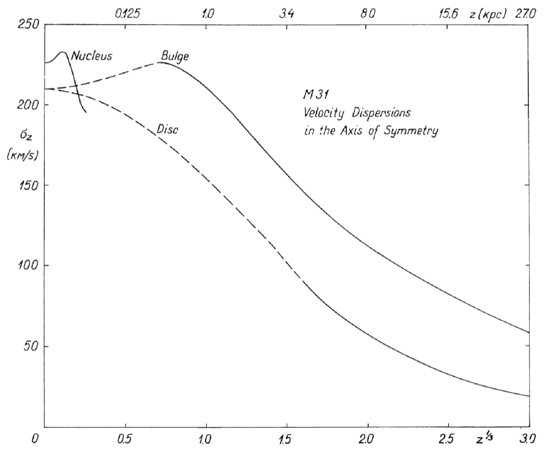
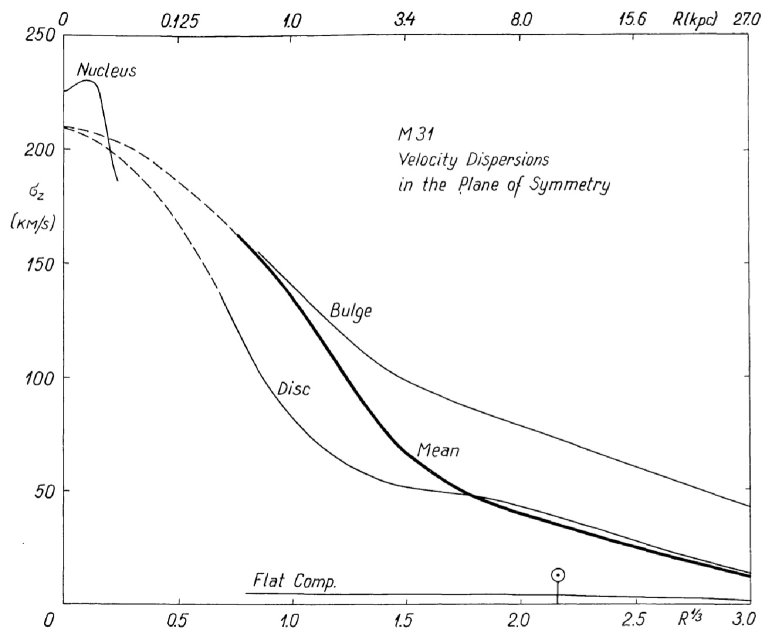
Figure 1: Left: Vertical velocity dispersion $\sigma_{z}$ of the components of M31 in the $z$-axis of symmetry. Right: Vertical velocity dispersion $\sigma_{z}$ of the components of M31 in the plane of symmetry.

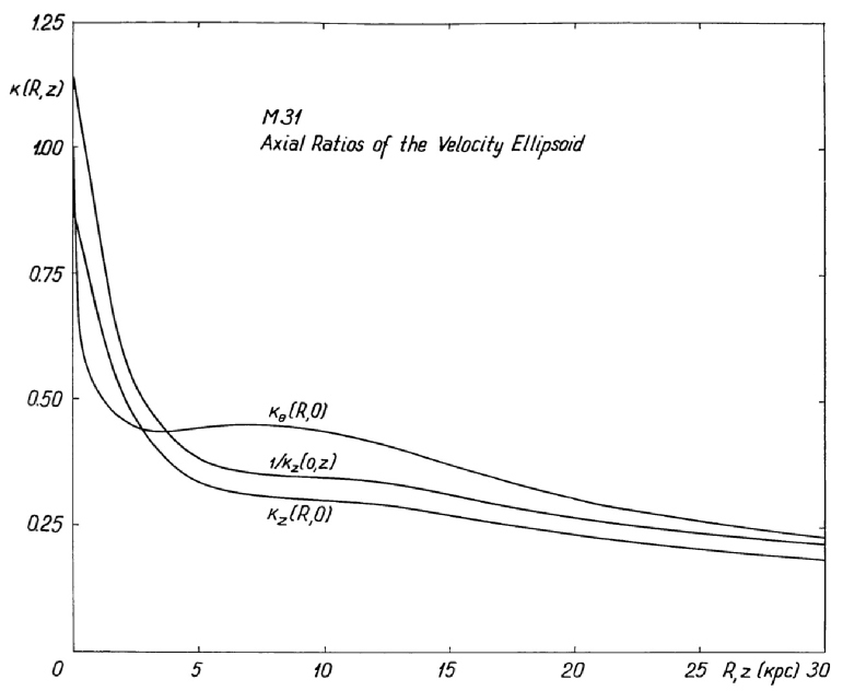
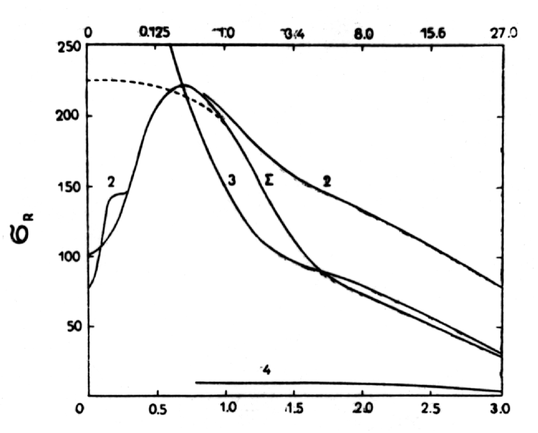
Figure 2: Left: Axial ratios of the velocity ellipsoid in the plane of symmetry and in the axis of M31. Right: Radial velocity dispersion $\sigma_{R}$ as function of $R$ for components of M31: 2 — bulge and halo; 3 — disc; 4 — flat; $\Sigma$ — galaxy as a whole. Horizontal scale is given in units $R^{1/3}$ and in $R$ on bottom and top, respectively.

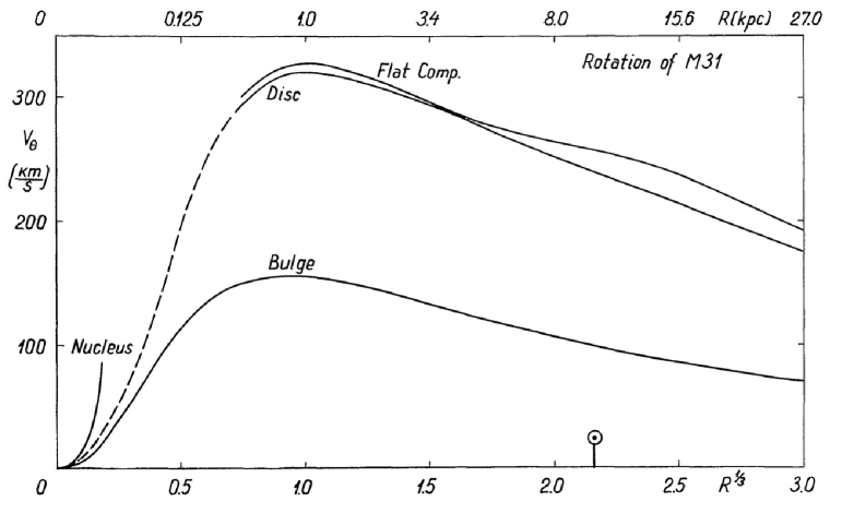
Figure 3: Rotation velocity $V_{\theta}$ for components of M31 in the plane of symmetry (Einasto & Rümmel 1970c).

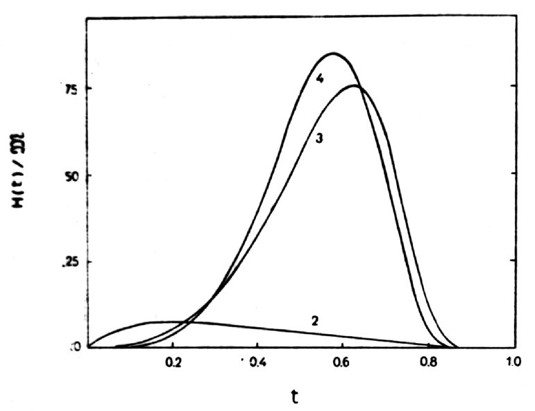
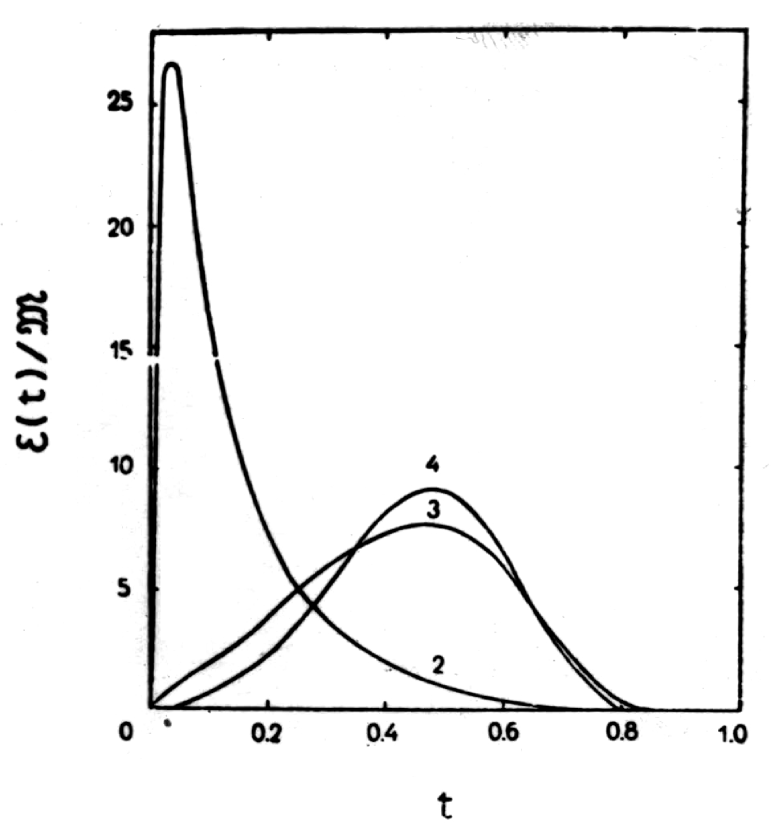
Figure 4: Left: A specific angular moment of components in units 100 km/sec per kpc. Right: Specific kinetic energy of M31 components in units $10^{4}$ (km/sec)², both are expressed as functions of $t=a/(1+a)$.

The derived parameters of the components are given in Table LABEL:Tab18.1.

To obtain better agreement with observations, the flat component of the galaxy has been represented by a sum of two functions (11), one of them being negative. This allows to describe the ring-like shape of the flat population with zero density at the centre. The parameters of this component are subject to the condition that the ring-like mass distribution has everywhere non-negative total density.

The mass of the nucleus has been determined by means of the virial theorem. In an earlier paper (Einasto 1969b), the mass has been found from the luminosity of the nucleus and its accepted mass-to-light ratio (Spinrad 1966). The mass $\mathfrak{M}\,=5.2\times 10^{8}\leavevmode\nobreak\ \mathfrak{M}\,_{\odot}$, obtained from the virial theorem for the nucleus, and the corresponding mass-to-light ratio $f=170$, does not agree with the value $f=17$, derived spectroscopically (Spinrad 1966). This discrepancy may be removed, supposing that the nucleus contains besides stars an invisible central body — a dead quasar (Lynden-Bell 1969). In this case, the virial theorem must be modified, and we get for the point mass $\mathfrak{M}\,=1.4\times 10^{8}\,\mathfrak{M}\,_{\odot}$, supposing $\mathfrak{M}\,=0.8\times 10^{8}\leavevmode\nobreak\ \mathfrak{M}\,_{\odot}$ for the mass of the stellar component of the nucleus.

4 Discussion

A. MASS DISTRIBUTION

Our model differs in two points from the models by Schmidt (1957b), Brandt & Scheer (1965), Roberts (1966) and Gottesman et al. (1966): the central concentration of mass is much higher, and the total mass smaller (Einasto 1969b), see Table LABEL:Tab18.1. The differences can be explained by various circular velocity curves adopted.

In the central region, the velocities found earlier from the 21-cm radio line measurements are underestimated due to the insufficient correction for the antenna smearing effect. The rotation velocities, derived optically for the stellar component of the galaxy, cannot be identified with the circular velocities, as the pressure term (velocity dispersions) in hydrodynamical equations is predominating.

The great masses are found in most cases as a result of approximation the observed rotation velocities with a generalised Bottlinger law

$$V_{\theta}={V_{0}\,R\over[1+(R/R_{0})^{n}]^{3/2n}},$$ (13)

where $V_{0}$ and $R_{0}$ are constants, and rotation velocity is identified with the circular velocity.

We have shown (Einasto 1969a) that the generalised Bottlinger law cannot be applied to the circular velocity, as in this case great masses at very large distances from the centre of the galaxy occur. This is impossible due to the tidal effect of nearby galaxies (King 1962).

The small radial gradient of the rotation velocity, observed in the periphery of some galaxies, in particular, in the Andromeda galaxy, is probably to be explained in another way, for instance, as the appearance of systematic streaming motion in the galaxy.

B. MASS-TO-LIGHT RATIO

The mean mass-to-light ratio found, $f=15.4$, is normal for a Sb galaxy. The flat population and the disc have also acceptable values, $f=2.5$ and $f=17.3$, respectively.

The mass-to-light ratio for the nucleus, $f=17.3$, seems to be too large at first glance. To explain this value, we must suppose that the nucleus: (a) consists of very old physically evolved stars, and (b) is dynamically not evolved.

The mean relaxation time of the nucleus is of the same order ($10^{10}$ yr) as the age of the whole galaxy. Therefore, the nucleus is dynamically indeed little evolved and has lost only a small fraction of his low-mass stars. As the nucleus has had too little time to form dynamically by star-star encounters, it must be formed in the protogalaxy stage of the galaxy evolution.

The metal content of stars in the nucleus is normal (Spinrad 1966). Therefore, if the high mass-to-light ratio and the great age of the nucleus will be confirmed, we must conclude that in the nucleus the metal enrichment has taken place in a very early stage of the galaxy evolution.

March 1969

Revised January 1970

Chapter 20 The spiral structure of M31

The density distribution and the radial velocity field in the Andromeda galaxy, M31, was studied on the basis of the 21-cm radio-line data from Jodrell Bank and Green Bank by Einasto & Rümmel (1970a), which forms Chapter 19 of the Thesis. The true density has been obtained from the observed one by solving a two-dimensional integral equation. As the resolving power of the radio telescopes is too low to locate all spiral arms separately, optical data on the distribution of ionised hydrogen clouds have also been used. The mean radial velocities have been derived by solving a two-dimensional non-linear integral equation with the help of hydrogen densities and a model radial velocity field.

The inner concentrations of hydrogen form two patchy ring-like structures with mean radii 30’ and 50’, the outer concentrations can be represented as fragments of two leading spiral arms.

The rotational velocity, derived from the radial velocity field, in the central region differs considerably from the velocity curves obtained by earlier authors. The difference can be explained by the fact that in this region, the correction for the antenna beam width is much greater than adopted by previous investigators.

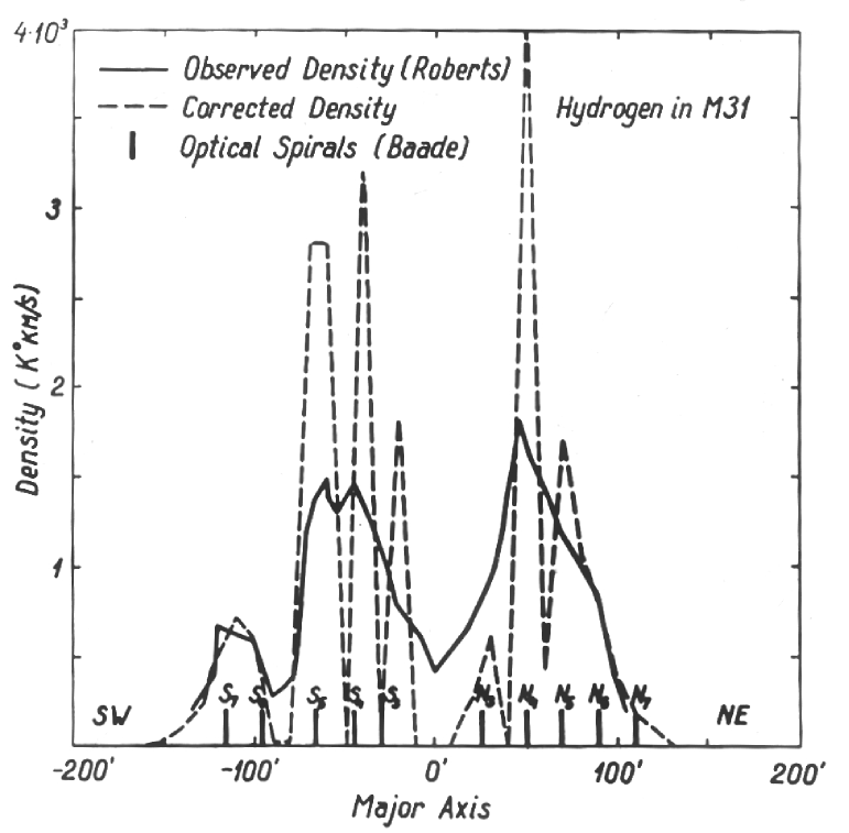
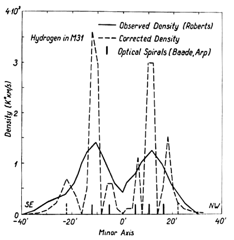
Figure 1: Left; Observed (Roberts 1967) and corrected distribution of projected density of neutral hydrogen along major axis of M31. Positions of optical spirals according to Baade & Arp (1964) are also shown. Right: Observed (Roberts 1967) and corrected distribution of projected density of neutral hydrogen along minor axis of M31. Positions of optical spirals according to Baade & Arp (1964) are also shown.

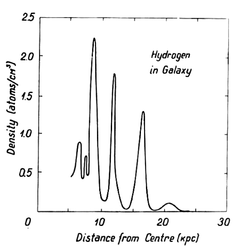
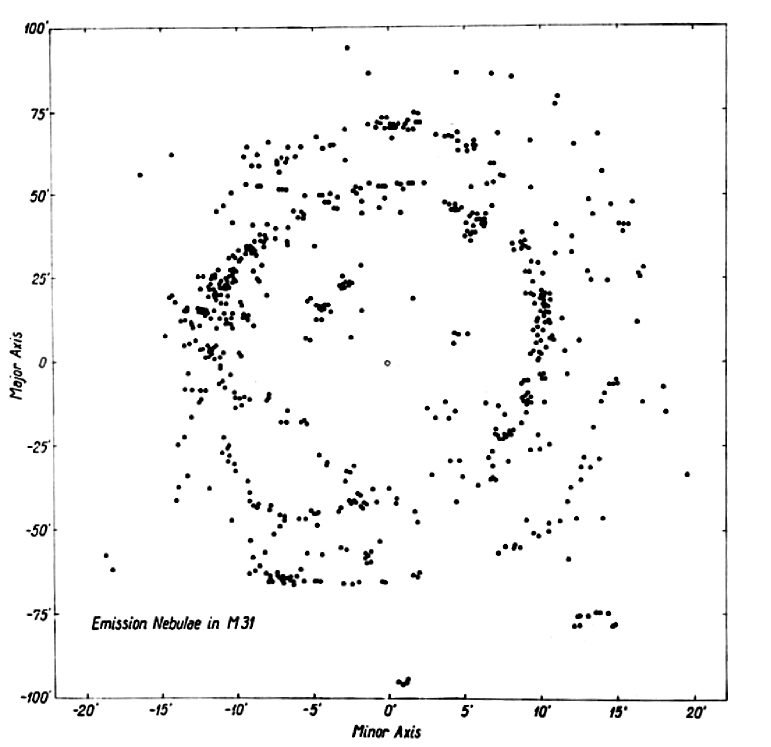
Figure 2: Left; Spatial density of neutral hydrogen in the Galaxy plane. Right: Distribution of ionised hydrogen clouds in M31 according to Baade & Arp (1964). The $X$-scale is enlarged by a factor of 4.5 to take into account the inclination of the plane.

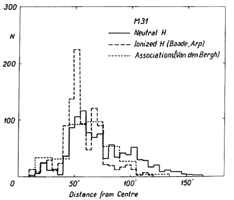
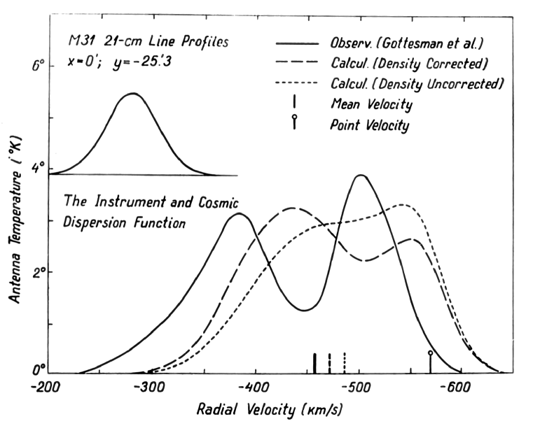
Figure 3: Left; Distribution of neutral and ionised hydrogen in M31 according to Baade & Arp (1964). Distribution of stellar associations according to van den Bergh (1964) is also shown. Right: Profiles of 21-cm lines for one point at the major axis of M31. The profile due to observational and “cosmic” errors is also shown.

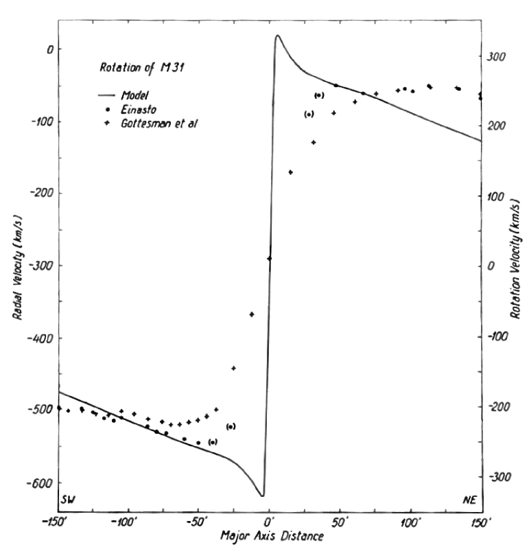
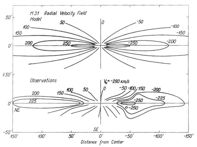
Figure 4: Left; Circular velocity of M31 according to models by Einasto & Rümmel (1970b) and Gottesman et al. (1966) and present work (Einasto 1972b). Right: The radial velocity field of M31 according to model by (Einasto 1972b) and observations.

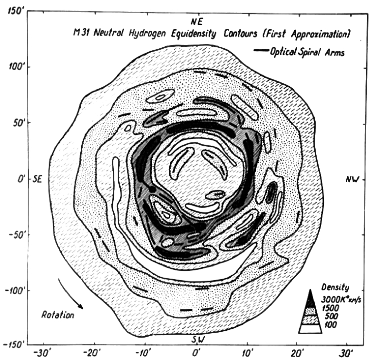
Figure 5: Equidensity contours of neutral hydrogen in M31.

1 Introduction

In the present paper, the density distribution and the radial velocity field of neutral hydrogen in the Andromeda galaxy, M31, have been studied. The investigation is based on the 21-cm radio-line data from Jodrell Bank and Green Bank Observatories, kindly sent to us by Dr. R. G. Davies and Dr. M. S. Roberts. Optical data on the distribution and motion of ionised hydrogen are also used.

When studying the distribution and motion of hydrogen in external galaxies, it is necessary to take into consideration the angular resolving power of radio telescopes. Gottesman et al. (1966) found that the correction for the beam width of the 250-feet Jodrell Bank telescope both in the density and the velocity does not exceed 10 %. Our calculations, however, have shown in some cases the correction needed is much greater. This indicates that the Jodrell Bank investigators have used a too simplified reduction method. The Green Bank data have been reduced neglecting the antenna smearing effect (Roberts 1966). For that reason, the available radio data are to be reduced once again. At present the program is not finished. In this paper the preliminary results are reported.

2 The integral equations for the density and the mean radial velocity

Let $X,Y$ be the rectangular galactocentric coordinates in minutes of arc, the $Y-$axis being directed to the NE side of the major axis of the galaxy; $V$ the true radial velocity; $D(X,Y)$ the true projected density of neutral hydrogen; $E(V-\overline{V})$ the distribution function of residual radial velocities in the direction $X$, $Y$; $\overline{V}=\overline{V}(X,Y)$ is the mean radial velocity in this direction.

The radio telescope, directed to the point $X_{p},\leavevmode\nobreak\ Y_{p}$ and disposed to the frequency, corresponding to the radial velocity $V_{k}$, will record the flux

$$\begin{array}[]{ll}T(X_{p},Y_{p},V_{k})&=\int\int\limits_{-\infty}^{\infty}\int\,D(X,Y)\,F(X-X_{p},Y-Y_{p})\\ &\times\,E[V-\overline{V}(X,Y)]\,G(V-V_{k}){\rm d}X\,{\rm d}Y\,{\rm d}V\,,\end{array}$$ (1)

where $F(X-X_{p},Y-Y_{p})$ is the angular sensitivity function of the telescope, and $G(V-V_{k})$ is the corresponding frequency sensitivity function.

Integrating (1) over all observed velocities $V_{k}$ we obtain the observed projected density of hydrogen $\overline{D}(X_{p},Y_{p})$, which is connected with the true density $D(X,Y)$ by means of the equation

$$\overline{D}(X_{p},Y_{p})=\int\int\limits_{-\infty}^{\infty}\,D(X,Y)\,F(X-X_{p},Y-Y_{p}){\rm d}X\,{\rm d}Y\,.$$ (2)

This is a two-dimensional homogeneous Fredhold integral equation of the first kind for the determination of the true density $D(X,Y)$. If the density is known, the Eq, (1) can be considered as a non-linear integral equation for the determination of the mean radial velocity $\overline{V}(X,Y)$.

The observations of point radio sources indicate that the function $F$ can be fairly well approximated by a two-dimensional Gaussian with half-intensity diameters 15’ and 10’ in the case of the Jodrell Bank and Green Bank telescopes respectively (Davies (1969) and Roberts (1969b)). The function $G$ has in the case of the Jodrell Bank telescope also a Gaussian shape with half-intensity width 200 kHz, which corresponds to a velocity dispersion of 17 km/s. The Green Bank telescope has a rectangular shaped function $G$ of 95 kHz (20 km/s) wide.

3 The density distribution

From the analogy with our Galaxy, we may expect that the neutral hydrogen in M31 is concentrated in spiral arms. The optical observations of ionised hydrogen (Baade & Gaposchkin 1963; Arp 1964b) indicate that the Andromeda galaxy has four to five spiral arms in both sides of the galaxy. The mean distance between every two arms is $20^{\prime}=4$ kpc, in projection only $4^{\prime}-8^{\prime}$, except the region around the major axis. The ionised hydrogen arms coincide with the neutral hydrogen arms within the actual distance of 5’; the neutral hydrogen arms are situated closer to the centre of the galaxy (Roberts 1967).

The resolving power of the radio telescopes used is not sufficient to separate all spiral arms in the Andromeda galaxy; only the most dense arms N4, S4 and S5 (designated after Baade & Gaposchkin (1963)) can be “seen” individually (Roberts 1967). To locate the outer neutral hydrogen arms, the optical data on the distribution of the ionised hydrogen clouds can be used (Baade & Arp 1964).

The true density distribution has been determined from the integral equation (2) by two methods. Near the minor axis, the equidensity lines are almost parallel to the major axis, and the two-dimensional equation can be reduced to the one-dimensional one. Representing the observed density distribution by a sum of Gaussian functions, we get the solution of the equation also in the form of a sum of Gaussian functions.

For points far off from the minor axis, the solution of the Eq. (2) has been found by successive approximations. The arms have been located by combining optical and radio data, the corrected densities have been derived from the observed radio densities by a trial-and-error procedure. The densities have been found for a network of points, placed in $X$ and $Y$ at intervals 2’ and 10’ respectively.

The observed (Green Bank) and corrected density profiles (first approximation) along the major and minor axes of the Andromeda galaxy are shown in Figures 1, left and right panels, respectively. The picture is quite similar to the neutral hydrogen density profiles found for our Galaxy; an example of them, drawn on the basis of the Dutch survey by Schmidt (1957a) and Westerhout (1957) is given in Fig. 2.

The $X,\leavevmode\nobreak\ Y$-distribution of ionised hydrogen clouds (Baade & Arp 1964) is given in the right panel of Fig. 2. The map of equidensity contours of neutral hydrogen is presented in Fig. 5. The $R$-distribution (integrated over all position angles $\theta$) of neutral and ionised hydrogen as well as of the stellar associations (van den Bergh 1964) is plotted in the left panel of Fig. 3. The original distributions are reduced to an equal total number of objects, $N=1000$.

The inspection of the data obtained leads us to the following conclusions:
(a) the spatial distribution of neutral hydrogen is similar to the distribution of ionised hydrogen and stellar associations; at great distances from the centre, the relative density of neutral hydrogen is higher than that of the ionised hydrogen;
(b) the inner concentrations of hydrogen form two patchy ring-like structures with the mean radii 30’ (the arms N3, S3 after Baade) and 50’ (the arms N4, S4);
(c) the outer hydrogen concentrations can be fairly well represented as fragments of two leading spiral arms S5-N6, N5-S6.

4 The radial velocity field

The density distribution function $D$ and the angular sensitivity function $F$ are independent of the velocity $V$, and in Eq. (1) we can integrate first over the velocity

$$\begin{array}[]{ll}T(X_{p},Y_{p},V_{k})&=\int\limits_{-\infty}^{\infty}\int\,D(X,Y)\,F(X-X_{p},Y-Y_{p})\\ &\times H[V_{k}-\overline{V}(X,Y)]{\rm d}X\,{\rm d}Y\,,\\ \end{array}$$ (3)

where

$$H[V_{k}-\overline{V}(X,Y)]=\int_{-\infty}^{\infty}\,G(V-V_{k})\,E[V-\overline{V}(X,Y)]{\rm d}V\,.$$ (4)

If the velocity dispersion is independent of position $X,\leavevmode\nobreak\ Y$, the Eq. (3) can be made more suitable for numerical computations. Let us use instead of $X,\leavevmode\nobreak\ Y$ the variables $S$, $\overline{V}$, where $S$ is the length along the line $\overline{V}(X,Y)=const$. We have

$$\begin{array}[]{ll}T(X_{p},Y_{p},V_{k})&=\int_{-\infty}^{\infty}\,H(V_{k}-\overline{V})\\ &\times\left[\int_{S}\,D(X,Y)\,F(X-X_{p},Y-Y_{p})\,J\left({X,Y\over S,\overline{V}}\right){\rm d}S\,\right]{\rm d}V\,,\end{array}$$ (5)

Assuming the Gaussian form both for the functions $G$ and $E$ with dispersions $\sigma_{G}$, $\sigma_{E}$, respectively, then the function $H$ has also the Gaussian form with the dispersion

$$\sigma_{H}^{2}=\sigma_{G}^{2}+\sigma_{E}^{2}.$$ (6)

Interferometric observations show (Deharveng & Pellet 1969) that the radial velocity dispersion has practically a constant value $\sigma_{E}=17$ km/s (due to the projection effect, the dispersion $\sigma_{E}$ is greater than the true radial velocity dispersion in a small volume element of the galaxy).

The formula (5) has been used to calculate the theoretical 21-cm line profiles. An effective radial velocity dispersion, $\sigma_{H}=24$ km/s, the corrected hydrogen density field, and a model radial velocity field have been used. The radial velocity field has been calculated from a plane disc pure rotation model, using the obvious formula

$$\overline{V}(X,Y)=V_{0}+V(R)\frac{Y}{R}\cos i,$$ (7)

where $V(R)$ is the circular velocity at the distance $R$ from the centre of the galaxy, $V_{0}$ — the mean radial velocity of the galaxy, and $i$ — the tilt angle of the plane of symmetry of the galaxy to the line of sight. The velocity $V(R)$ was taken from our four-component model of the Andromeda galaxy (Einasto & Rümmel 1970b), the constants are chosen as follows: $i=12.^{\circ}8$, $V_{0}=-300$ km/s.

Gottesman et al. (1966) derived for 231 points $X_{p},\leavevmode\nobreak\ Y_{p}$ the line profiles (spectra) $T(V_{k}|X_{p},Y_{p})$. For all these points, the theoretical profiles have been calculated. These are quite similar to the observed profiles but, in general, shifted in the velocity. The comparison of the profiles enables us to correct the model radial velocity field.

In this way, we have found a solution to the integral equation (1). From the corrected radial velocities near the major axis points, a new improved rotation velocity curve has been derived.

The results are presented graphically. In the right panel of Fig. 3 the 21-cm line profiles for a major axis point are given. The theoretical profiles are calculated by using both the corrected and uncorrected (observed) hydrogen densities, the model velocity field being identical. Mean radial velocities and the point velocity $V_{p}$ (the model radial velocity at the point $X_{p},Y_{p}$) are also indicated. In Fig. 4 the rotation curves are presented, and in the right panel of Fig. 4 the model and observed radial velocity field.

The analysis of the results can be summarised as follows:
(a) the change of the density causes both vertical and horizontal shifts in the line profiles, therefore, an unbiased radial velocity field can be derived only by using carefully corrected densities;
(b) when the radio telescope is directed to a point of low hydrogen density or large density gradient, the mean radial velocity of the profile does not coincide with the point velocity; in extreme cases near the major axis the difference exceeds 100 km/s. This effect has caused large systematic errors in the previous reductions of radio data by Argyle (1965), Gottesman et al. (1966) and Roberts (1966);
(c) the corrected radial velocity field has great irregularities in respect to the model field.

July 1969

Chapter 21 Structural and kinematical properties of M31 populations

This Chapter presents our second attempt to construct a model of the Andromeda galaxy M31. It was developed step-by-step, adding more data on structural and kinematical properties of populations. It was presented in IAU Symposium on “External galaxies and quasi-stellar objects”, held in Uppsala August 10 - 14, 1970, and published by Einasto (1972b). Here the model is presented according to the Thesis version of the Chapter, using also data and text of the Symposium version.

1 Introduction

To construct a meaningful physical theory of the structure and evolution of a galaxy, one needs reliable data on parameters, describing the spatial and kinematical structure of the galaxy and its subsystems of different ages. As such parameters one can adopt: the mass of the subsystem $\mathfrak{M}\,$, its mean radius $a_{0}$, the axial ratio of equidensity ellipsoids $\epsilon$ (supposing equidensity surfaces of subsystems to be ellipsoids of rotational symmetry and constant axial ratio), and suitable structural parameters determining the degree of concentration of the mass to the centre of the system. As morphological parameters, we can consider colour and mass-to-light ratio of subsystems. As descriptive functions, we can use spatial density $\rho$, projected luminosity $L$, circular velocity $V$, rotational velocity $V_{\theta}$, velocity dispersions $\sigma_{R},\leavevmode\nobreak\ \sigma_{\theta},\leavevmode\nobreak\ \sigma_{z}$, and some others.

In a series of papers, Einasto (1969a) and Einasto & Rümmel (1970b, a, c) studied the structure of the Andromeda galaxy and its subsystems, and calculated preliminary values for descriptive parameters. Recently, new observational data have become available for the nucleus, the subsystem of globular clusters, and interstellar hydrogen. It appears reasonable to use these data to redetermine structural parameters of the populations. Also the reconstruction of the physical evolution of galaxies was made on the basis of the theory of evolution of stars of different mass and composition, described in the following Chapters. This allowed to calculate structural and kinematical parameters of subsystems of the Andromeda galaxy M31, and to construct its new model. Preliminary results of this work were published by Einasto (1972b), here we describe the new model in more detail.

2 Reddening and luminosity dimming of M31

Einasto (1969b) did not correct data for the reddening effect, Einasto (1972b) used for correction data by Arp (1965). A collection of reddening determinations is given in Table LABEL:Tab20.1, where we show the colour excess $E(B-V)$ of various objects in M31 and its vicinity.

Table 1: Reddening determinations in M31

Object	$E(B-V)$	References
Halo clusters	$0.08\pm 0.02$	van den Bergh (1969)
Field stars	$0.11\pm 0.02$	McClure & van den Bergh (1968)
Blue open clusters	$0.12\pm 0.04$	Schmidt-Kaler (1967)
Nucleus	0.13	Einasto (1972b)
Nucleus	0.20	Arp (1965)
Cepheids	$0.16\pm 0.03$	Baade & Swope (1963)
Cepheids	0.15	van den Bergh (1968)
Mean M31	$0.17-0.20$	Einasto (1972b)

The colour excess $E$ was determined as follows. Data by van den Bergh (1969), Kinman (1965), Lallemand et al. (1960), Sandage et al. (1969) suggest that the apparent colour excess of the nucleus of M31 is $B-V=1.04$ and $U-B=0.78$, a mean colour excess of galaxies of Sb type is $B-V=0.97$, $U-B=0.59$ (de Vaucouleurs 1961), which gives $E(B-V)=0.07$ and $E(U-B)=0.19$. The colour excess $E(U-B)$ can be found from $E(B-V)$, using the relation $E(U-B)/E(B-V)=0.72$, which yields $E(B-V)=0.26$. The mean value is $E(B-V)=0.13$, giving double weight to the direct estimation of $E(B-V)$. de Vaucouleurs (1961) gives for the galaxy M31 as a whole $B-V=0.91$ and $U-B=0.50$, and as a mean for Sb galaxies $B-V=0.81$ and $U-B=0.27$, which gives a value $E(B-V)=0.17$.

A slightly larger value was found in a different way. Schmidt-Kaler (1967) used to find $E(B-V)$ the most blue clusters of M31, which did not have reddening within M31, but only within the Galaxy. The reddening in the Galaxy can be found also using halo clusters (van den Bergh 1970) and field stars (McClure & van den Bergh 1968). On the basis of these data, we find that the reddening in the M31 direction within our Galaxy is $E(B-V)=0.10\pm 0.02$. On the other hand, according to Sharov (1968b), the mean reddening in the line of sight within M31 is $A_{V}=1$. If we assume that the reddening within M31 is due to a thin layer of dust near the symmetry plane, then objects within M31 can be divided into two classes, nearby ones with no reddening, and more distant ones with reddening $A_{V}=1$. As the mean we get $A_{V}=0.39$ and $E(B-V)=0.13$. However, some reddening occurs in spiral arms, thus outer regions of M31 have smaller reddening. Taking these considerations into account, we accept the mean reddening within M31 $E(B-V)=0.10$, and together with the reddening within our Galaxy $E(B-V)=0.20$.

This overview shows that the light of different M31 subsystems is influenced by reddening differently. As a mean reddening, we accept $E(B-V)=0.15$, which is twice less than accepted by Einasto (1972b). Using the apparent distance modulus (after cepheids) $(m-M)_{0}=24.2$ and $R=A_{V}/E(B-V)=3$ we get for the true distance modulus $(m-M)_{0}=24.2\pm 0.05$.

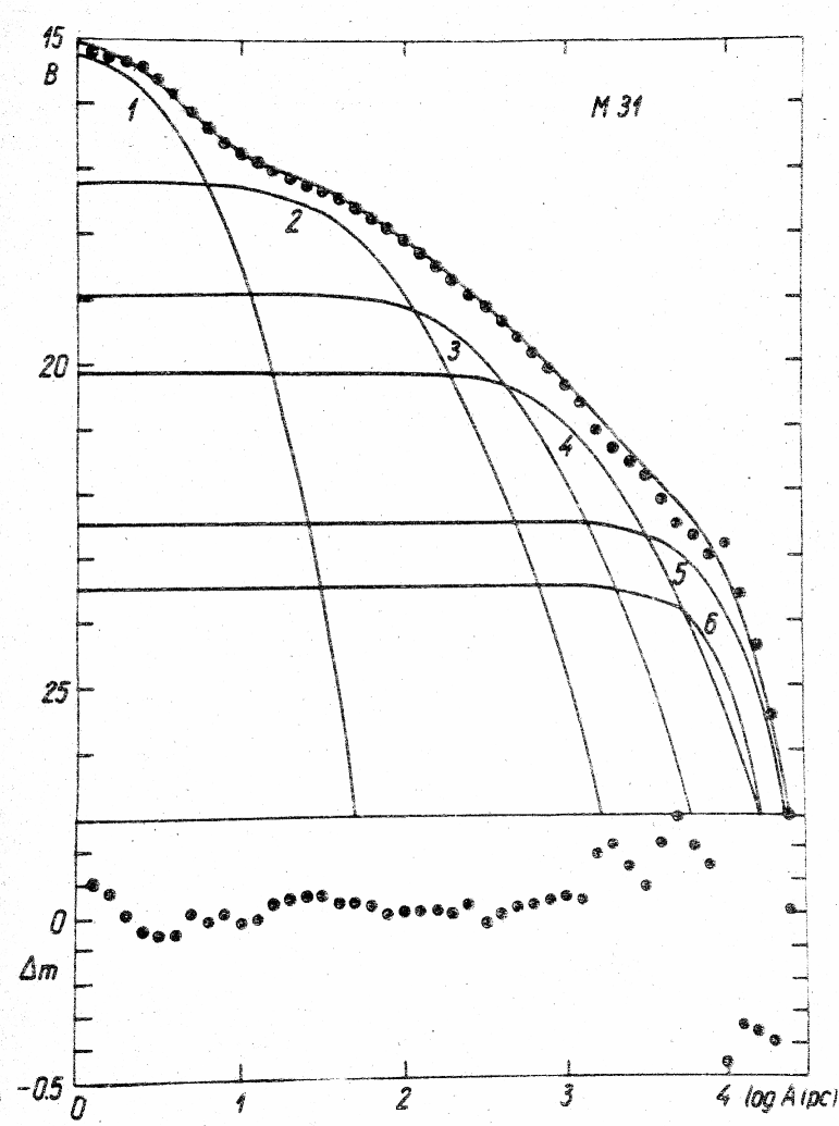
Figure 1: Luminosity profile of M31 in photometric system B is shown by a bold curve, profiles of components by thin curves. The lower panel shows the difference $\Delta\,m=B_{Obs}-B_{Mod}$. Components are: 1 – nucleus, 2 – core, 3 – bulge, 4 – halo, 5 – disc, 6 – flat.

3 New model of M31

In the new model, we used the photometrical profile in B system by Einasto (1969b), using additional data to calculate improved parameters of the M31 model. Parameters of the new model are given in Table LABEL:Tab20.2, the new photometric profile in Fig. 1, and new axial ratio data in Table LABEL:Tab20.2. We shall discuss details on individual populations below. Here we consider principal model parameters.

In addition to photometrical and kinematical data used earlier (Einasto 1969b; Einasto & Rümmel 1970a), we now used the following new data: spectro-photometrical and photometrical data on the stellar content (van den Bergh (1970), Sandage et al. (1969), Spinrad (1966); Spinrad & Taylor (1969); Spinrad et al. (1970), McClure & van den Bergh (1968) and de Vaucouleurs (1969)), kinematical data on globular clusters (van den Bergh 1970) and interstellar hydrogen (Deharveng & Pellet (1969) and Rubin & Ford (1970)). Additionally, we used our results on the physical evolution of galaxies, discussed in Chapter 22.

The main difficulty in the determination of parameters of our preliminary models was related to calculations of mass-to-light ratios of populations. New data allow to find more accurate values of these parameters.

In Chapter 22,, we discussed three variants on the star formation function with $S=0,\leavevmode\nobreak\ 1$ and 2. To apply results of Chapter 22 to study the structure of M31 we must have a choice between these parameter values.

The mass of the neutral hydrogen in M31 can be taken equal to $\mathfrak{M}\,_{H_{I}}=3.7\times\,10^{9}\leavevmode\nobreak\ M_{\odot}$ (Argyle (1965), Gottesman et al. (1966) and Deharveng & Pellet (1969)), using for the distance $d=690$ kpc. The mass of ionised hydrogen is less by several orders, and the total mass of interstellar matter is $\mathfrak{M}\,_{G}=5.3\times 10^{9}\,M_{\odot}$, if we accept normal chemical abundance with $X=0.70$. If we accept the total mass of the M31 $\mathfrak{M}\,_{t}=218\times\,10^{9}\,M_{\odot}$ according to Einasto (1972b), then we get for the mass of the gas $\mathfrak{M}\,_{G}=0.024\,\mathfrak{M}\,_{t}$. If we neglect the gas, expelled from stars during their evolution, and take the total age of M31 equal to $10^{10}$ years, then with the exponential decrease of gas mass ($S=1$), this gas fraction corresponds to star formation function parameter $K=2.7\times\,10^{9}$ yr. If we use $S=2$, we get for the characteristic time $K=0.25\times\,10^{9}$ yr.

In our model, the flat component has $\epsilon=0.02$, and the disc has $\epsilon=0.08$. We can attribute all populations with $\epsilon<0.4$ to the flat component, with a maximal age $1.7\times 10^{9}$ yr according to Einasto (1970a). During last billions of years, the star formation rate in galaxies like M31 was approximately constant, and we get using data from Chapter 22 for the mass-to-light ratio $f_{B}=0.43$. The total mass of stars formed during last $1.7\times 10^{9}$ yr is $\mathfrak{M}\,_{S}=4.7\times 10^{9}\,M_{\odot}$, and luminosity $L_{S}=10.9\times\,10^{9}\leavevmode\nobreak\ L_{\odot}$, if we accept $S=1$ and $K=2.7\times 2.7\times 10^{9}$ yr. For $S=2$ and $K=0.25\times 10^{9}$ yr we get $\mathfrak{M}\,_{S}=1.06\times 10^{9}\leavevmode\nobreak\ M_{\odot}$ and $L_{S}=2.46\times\,10^{9}\leavevmode\nobreak\ L_{\odot}$. According to Einasto (1969b) the total luminosity of the flat component is $L_{B}=3.0\times 10^{9}\leavevmode\nobreak\ L_{\odot}$ (using $E(B-V)=0.15$). This comparison suggests that the model with $S=2$ agrees much better with observations.

Using data given in Chapter 22, we find that the mass-to-light ratio of the whole galaxy is $f_{B}=9.5$, when we accept normal solar composition $Z=0.02$, $S=2$, $T_{G}=10\times 10^{9}$ yr, and star formation parameter $K=0.25\times 19^{9}$. From observations, using $E(B-V)=0.15$, we get $f_{B}=11.08$, which corresponds to composition with a slightly higher metal content. This result is expected, since according to Spinrad & Taylor (1969) the metal content in our Galaxy is slightly higher than the solar content, and according to van den Bergh (1969) the metal content in M31 is higher than in the Galaxy.

Calculations by Cameron & Truran (1971) demonstrate that the metal-enrichment of interstellar gas with heavy elements was very rapid in the early phase of the evolution of the Galaxy. In later stages of the evolution, the chemical content was almost constant with time. For this reason, we can accept that the chemical composition of flat and disc components did not change with time, and that this content is representative for the whole galaxy. In this case we can take that the sum of the flat and disc components, as well as the galaxy as a whole, have constant ratio $f_{B}$. Accepting the values given above for the mass of the interstellar matter and the mass and luminosity of young stars, we get for the mass of the flat component $\mathfrak{M}\,_{F}=6.36\times 10^{9}\leavevmode\nobreak\ M_{\odot}$, and luminosity $L_{F}=2.4\times 10^{9}\leavevmode\nobreak\ L_{\odot}$. For the disc, we have the luminosity from the photometric profile, $L_{D}=7.57\times 10^{9}\leavevmode\nobreak\ L_{\odot}$, and for the summed luminosity of the disc and flat components: $L_{FD}=10.03\times 10^{9}\leavevmode\nobreak\ L_{\odot}$, which yields $f_{B}=11.08$, and mass of these components, $\mathfrak{M}\,_{FD}=112.2\times 10^{9}\leavevmode\nobreak\ M\odot$.

Now we consider data on spherical components. New data suggest that in these components, there exist large local anomalies in the chemical composition. For this reason, we cannot consider this component as a homogeneous one. Our data suggest that the spherical population can be well described by three sub-systems. The inner-most subsystem has chemical composition and mass-to-light ratio $f_{B}$, similar to the nucleus (Spinrad et al. 1971). For the intermediate subsystem (bulge), we accept a normal chemical composition and $f_{B}$, and for the most extended subsystem (halo) we accept chemical composition and $f_{B}$, close to that of halo globular star clusters. After several trials, we accepted mass and mass-to-light parameters, given in Table LABEL:Tab20.2. Following Einasto (1972a, 1974a) we designate the inner bulge as the core. Einasto (1972b) calculated preliminary versions of mass-to-light ratios and masses for components, used to prepare Fig. 6, and listed in Figure caption.

Table 2: Parameters of the components of M31

Quantity	Unit	Nucleus	Core	Bulge	Halo	Disc	Flat	Total
$\epsilon$		0.80	0.80	0.80	0.30	0.08	0.02
$\nu$		1/2	1/4	1/4	1/4	1	2
$a_{0}$	kpc	0.005	0.15	0.8	3	9.2	8
$L_{B}$	$10^{9}\,L_{\odot}$	0.0057	0.501	2.94	6.18	7.57	2.46	19.65
$L_{V}$	$10^{9}\,L_{\odot}$	0.0073	0.642	3.63	6.34	9.08	1.88	21.57
$\mathfrak{M}\,$	$10^{9}\,M_{\odot}$	0.306	27.0	58.4	19.8	105.8	6.36	217.7
$f_{B}$		53.8	53.8	19.88	3.20	13.98	2.59	11.08
$f_{V}$		42.0	42.0	16.09	11.66	3.39	3.39	10.09
$U-B$		0.67	0.65	0.47	0.16	0.43	$-0.17$
$B-V$		0.89	0.89	0.85	0.65	0.82	0.33	0.72

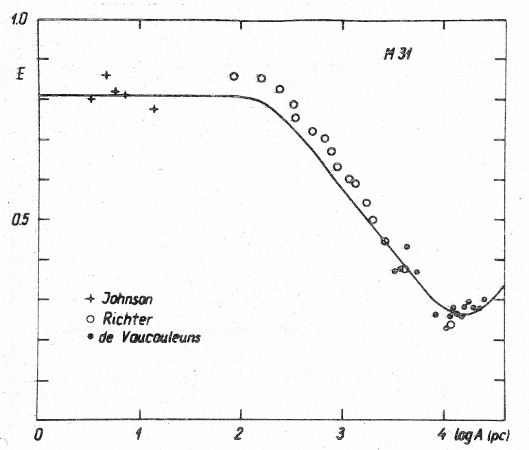
Figure 2: The apparent axial ratio of isophotes $E$ as function of the distance along major axis $A$. The curve is as found in our model, symbols show observational determinations.

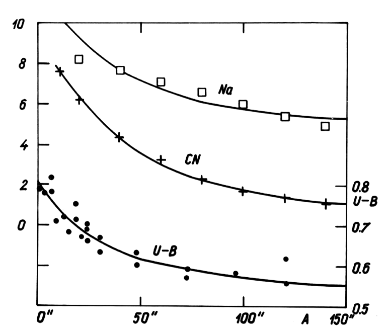
Figure 3: Colour $U-B$ and the intensity of spectral features $N\alpha$ and $CN$ in central region of M31 as functions of the distance from the centre $A$. Model curves were found under the assumption that subcomponents 1 and 2 (nucleus and core) have a composition, rich in heavy elements, and the bulge has normal composition.

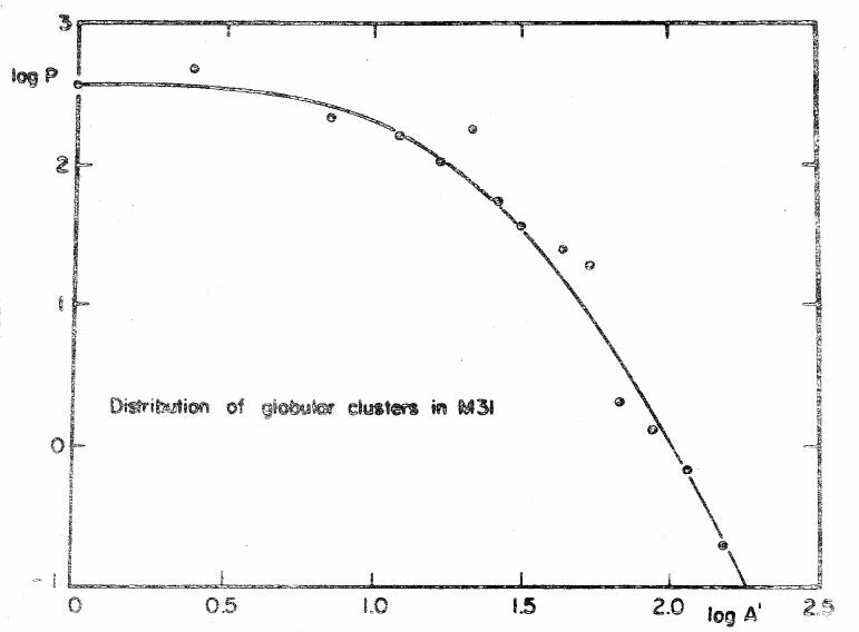
Figure 4: The distribution of globular clusters in M31.

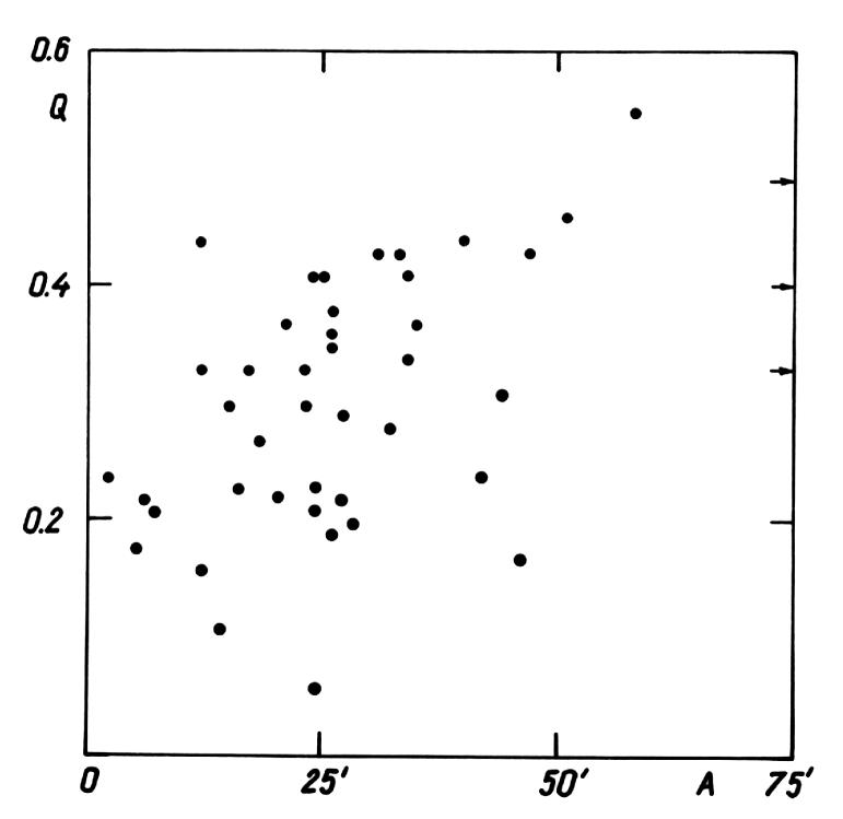
Figure 5: The dependence of the metallicity parameter $Q$ of M31 globular clusters on the distance from the centre $A$.

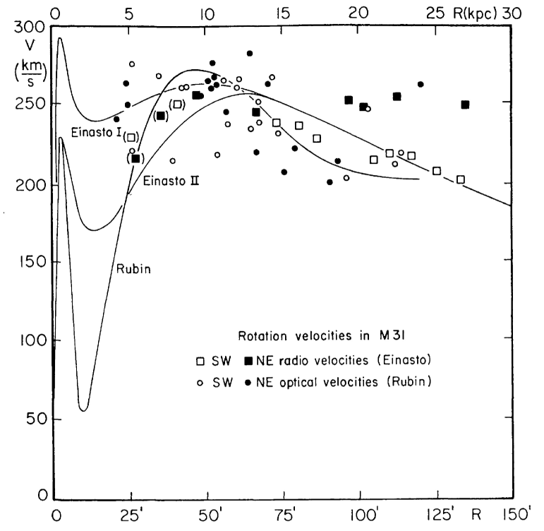
Figure 6: The rotation curve of M31. Observed rotation data from optical and radio measurements according to a summary by Rubin & Ford (1970) are shown by various symbols. Solid curves show rotation according to the model by Rubin & Ford (1970), and two variants of the model by Einasto (1972b). In this model mass-to-light ratios $f_{V}$ of nucleus, bulge, halo, disc and flat populations are in variant I – 42,  4.2, 4.1, 10.1, 3.2, and in variant II – 42, 2.7, 0.07, 14.7, 6.5.

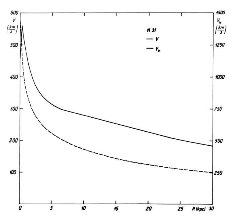
Figure 7: Circular and escape velocities, $V$ and $V_{k}$ of M31 as functions of distance from the centre $R$ according to the model by Einasto (1972b).

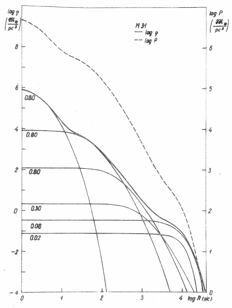
Figure 8: Distribution of the projected density of M31 and its components.

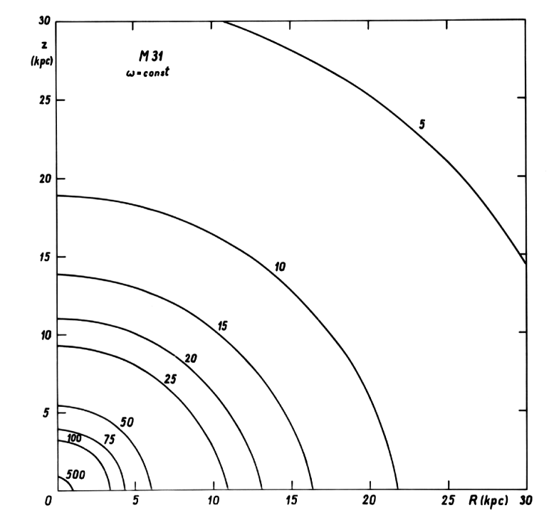
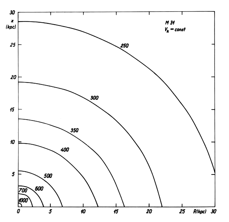
Figure 9: Left and right panels show isolines of M31 angular velocity $\omega$ and escape velocity $V_{k}$, respectively.

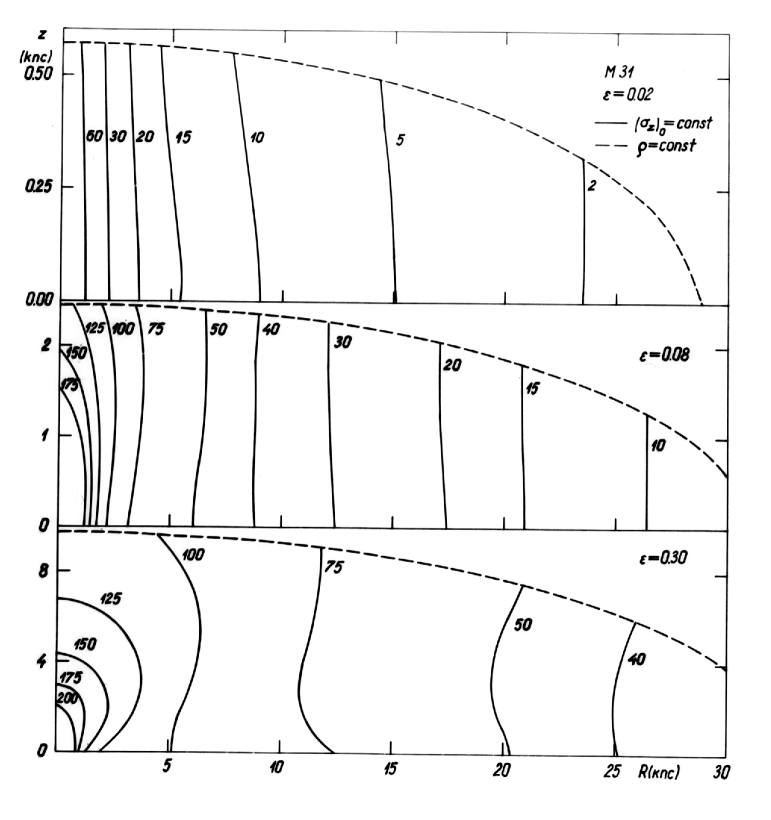
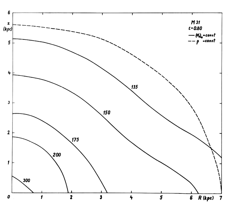
Figure 10: Top: Isolines of velocity dispersion $\sigma_{z}(R,z)$ and density $\rho(R,z)$ in the meridional plane $R,z$ of M31 for three test populations of flattening $\epsilon=0.02,\leavevmode\nobreak\ 0.08,\leavevmode\nobreak\ 0.30$. Bottom: Similar isolines for $\epsilon=0.80$. For explanations see Chapter 7.

The colour index of the nucleus and inner components of spherical components (core and bulge) were found from photometric observations by Lallemand et al. (1960), de Vaucouleurs (1961), Kinman (1965) and Sandage et al. (1969). For other components, there are no direct observational data, and colours were calculated using the theory of the evolution of integral colours of components, as described in Chapter 22.

Luminosities, effective radii and axial ratios of components were found from photometric data. The radius of the metal-rich inner spherical component (subpopulation 2 — core) was found from spectrophotometric data by Spinrad et al. (1971). To get in the model the minimum of the isophote axes ratio function, similar to the observed minimum (see Fig. 2), the axial ratio of the halo was decreased to $\epsilon=0.30$, and of the disc to $\epsilon=0.08$. Also, it was needed to decrease the angle between the system plane and line of sight from $i=12.^{\circ}7$ to $i=12.^{\circ}5$.

Using the virial theorem and hydrodynamical model for all subsystems, mean velocity dispersions $\sigma_{R},\leavevmode\nobreak\ \sigma_{z},\leavevmode\nobreak\ \sigma_{r}$ were calculated. Velocity dispersions $\sigma_{z}(R,z)$ of four populations in the meridional plane are shown in Fig. 10.

4 Nucleus

At the Basel IAU Symposium on Spiral Structure of the Galaxy, we argued that different methods lead to different values for the mass of the nucleus of M31 (Einasto & Rümmel 1970c). On the basis of photometric data by Redman & Shirley (1937), Johnson (1961), and Kinman (1965), and spectrophotometric data on the stellar content and mass-to-light ratio, $\mathfrak{M}\,/L=f=16$ (Spinrad 1966) we obtained (Einasto 1969b) for the mass of the nucleus the value $\mathfrak{M}\,=5\times\,10^{7}\leavevmode\nobreak\ M_{\odot}$. On the other hand, the known mean radial velocity dispersion of stars in the nucleus is $\sigma_{r}=225$ km/sec (Minkowski 1962), the mean radius is $a_{0}=5$ pc (obtained from photometric profile of the nucleus), and axial ratio of equidensity ellipsoids is $\epsilon=0.8$. These data enable us to apply the tensor virial theorem (see Chapter 12), which yield for the mass $\mathfrak{M}\,=5\times 10^{8}\leavevmode\nobreak\ M_{\odot}$ (Einasto & Rümmel 1970c).

The discrepancy in mass can be removed supposing, as Lynden-Bell (1969) does, that a massive body exists in the centre of the galaxy. In this case, the tensor virial theorem is to be modified. For the mean radial velocity dispersion of stars in the nucleus we have

$$\overline{\sigma}_{r}^{2}=Ga_{0}^{-1}\beta_{r}(\mathfrak{M}\,_{C}+H_{0}\,\mathfrak{M}\,_{0}),$$ (1)

where $G$ is the gravitational constant, $a_{0}$ is the harmonic mean radius of the stellar subsystem of the nucleus, $\mathfrak{M}\,_{C}$ and $\mathfrak{M}\,_{0}$ are masses of the central body and the stellar population of the nucleus, respectively, and $H_{0}$ and $\beta_{r}$ are dimensionless parameters. From photometric observations, we get for the nucleus $\epsilon=0.8$, and $i=12.^{\circ}8$, which gives $\beta_{r}=0.375$. The spatial density of stellar population of the nucleus can be well represented by the exponential model, for which $H_{0}=0.312$. Adopting for the mean radius and the mass of the stellar component the values given above, we obtain for the central mass $\mathfrak{M}\,_{C}=1.4\times 10^{8}\leavevmode\nobreak\ M_{\odot}$.

After the Basel Symposium, I asked Dr. H. Spinrad to determine the maximum value of mass-to-light ratio, consistent with spectroscopic observations. Recently new data became available (Spinrad & Taylor 1971). According to the new model of the stellar content, the mass-to-light ratio increases to a value of $f_{V}=42$, due to the necessity of adding faint M dwarfs. An upper limit to the number of red dwarfs is given by $V-K,V-L$ colour observations (Sandage et al. 1969), which gives $f_{V}\leq 65$.

A re-examination of the photometric data mentioned above gives for the luminosity of the nucleus in visual light a value $L_{V}=1.42\times 10^{7}\leavevmode\nobreak\ L_{\odot}$. This is four times higher than our previous estimate. The difference is due to the absorption and colour corrections: $A_{V}=0.6$ in our Galaxy, $A_{V}=0.3$ in M31 (Arp 1965), and $B-V=1.0$ (Sandage et al. 1969). The luminosity profile of M31 is shown in Fig. 1. Using these data, we obtain for the mass of the stellar component of the nucleus $\mathfrak{M}\,_{0}=6.4\pm 2.1\times 10^{8}\leavevmode\nobreak\ M_{\odot}$, accepting $E(B-V)=0.3$). On the other hand, on the basis of the virial theorem we get $\mathfrak{M}\,_{0}=5.7\pm 1.9\times 10^{8}\leavevmode\nobreak\ M_{\odot}$ (using $\mathfrak{M}\,_{C}=0$).

Good agreement between these two independent estimates shows that it is not necessary to suppose the existence in the centre of M31 of a body of large mass. However, ultraviolet observations carried out from the OAO indicate the presence of a UV-source in the nucleus of M31. If this source has small dimensions compared with the mean radius of the stellar component of the nucleus, Eq. (1) may be applied to estimate an upper limit for the point mass, which may be attributed to the UV-source. Assuming $\mathfrak{M}\,_{0}\geq 4.0\times 10^{8}\leavevmode\nobreak\ M_{\odot}$, we find $\mathfrak{M}\,_{C}\leq 0.5\times 10^{8}\leavevmode\nobreak\ M_{\odot}$. Thus, presently available data are not sufficient to confirm the presence of a point-like mass in the centre of M31. However, indirect data (recent explosion of the M82 galaxy) make the existence of such a body very likely in galaxies of type Sb.

Sandage et al. (1969) concluded from the $U-B$ colour variation along the major axis that the stellar content of the nucleus differs from that of the bulge. However, at present it is not clear whether the variation is due to a difference in stellar content or to the existence of a non-stellar UV-source in the centre of M31. A difference in stellar content is not excluded because the nucleus is dynamically almost isolated and there is no appreciable exchange of stars between the nucleus and the bulge.

Table 3: Apogalactic distances from the nucleus centre

$V$ (km/sec)	$R_{apogal}$ (pc)
225	1.8
450	8
1080	85

A rather great difference in chemical composition of stars on various distances from the centre of galaxies raises the question: Can this difference have a permanent character or will it change with time due to a mixture of stellar orbits? If most stellar orbits in the central region are radially extended, then stars in different regions will be mixed. However, our calculations showed this does not occur with stars of the nucleus as well with stars of inner region of the halo. In other words, stellar populations in different subsystems are dynamically isolated. To demonstrate this, we calculated, with the aid of a model of the mass distribution and the gravitational field of the nucleus, the apogalactic distances of stars moving through the centre of the nucleus with various velocities, see Table LABEL:Tab20.4. The majority of the nucleus stars have velocities of some hundred km/sec and do not move far off from the centre. Only stars having large velocities exceeding the escape velocity with respect to the nucleus, 1080 km/sec, go far away.

The mass density near the centre of M31 according to our model is $2\times 10^{6}\leavevmode\nobreak\ M_{\odot}$ pc^-3, the angular velocity is 12 km/sec/pc (Lallemand et al. 1960). Using the tensor virial theorem and supposing a rigid-body rotation, we find that the rotation energy is only 7.5 % of the total kinetic energy of the nucleus. The binding energy of the nucleus (total negative energy per unit mass) is $7.5\times 10^{4}$ (km/sec)².

5 Bulge

The bulge is the densest component of spheroidal populations of spiral galaxies, the characteristic radius of the bulge of M31 is of the order of 1 kpc. Photometrical data suggest that the bulge is fairly homogeneous. However, spectrophotometric data indicate that there exist differences in chemical composition (Sandage et al. (1969), Spinrad & Taylor (1971) and Spinrad et al. (1971)). Chemical composition influences mass-to-light ratios. Data by Spinrad et al. (1971) suggest that in the inner part of the bulge (at distance 1’ from the centre of M31) $f_{V}=45$, but data by Tinsley & Spinrad (1971) suggest $f_{V}=9.2$. If we attribute for the whole bulge $f_{V}\approx 40-50$, we get for the mass of the bulge an absurd value, larger than the mass of the whole galaxy M31. On the other hand, there is no doubt that the inner part of the bulge has high value of $f_{V}$. For this reason, we divide the bulge into two subsystems.

In the choice of $f_{V}$ for the inner bulge, we shall use the value $f_{V}=42$. If we accept the value $f_{V}=92$, suggested by Tinsley & Spinrad (1971), then we get for this subsystem velocity dispersion $\sigma_{r}=450$ km/sec, which is too high.

Earlier we assumed (Chapter 17) that velocity dispersion can have a minimum near the centre of the system. Later calculations (Chapter 18) suggested that this is possible only in the case when the increase of the density towards the centre is rather modest. The projected luminosity function has near the centre of M31 a high maximum, as in other spiral and elliptical galaxies. The minimum in the velocity dispersion near the centre can be avoided only in case the mass-to-light ratio in central regions is much lower than in the galaxy as a whole. Actually, this is not the case, thus a minimum of the velocity dispersion near the centre is unavoidable. This minimum is not very deep, as suggested in our earlier model of M31, described in Chapters 17 and 18.

We determined the radius of the inner bulge using data on the chemical composition of M31 (Sandage et al. (1969) and Spinrad et al. (1971)). In Fig. 3 we show the colour $U-B$, index $Na$ and $CN$ according to model (curve) and data (points).

There are no direct data on the chemical composition and mass-to-light ratio for the outer component of the bulge. We accepted for this component normal chemical composition, colour and parameters $f_{B}$ and $f_{V}$, using data of calculations of the evolution in Chapter 22. Comparison with parameters of other components of the galaxy, and the virial theorem suggest that parameters accepted for this component cannot have large errors.

6 Halo

The halo is the outer subsystem of the spherical component of galaxies. We found the effective radius, total luminosity and the axial ratio from photometric data and colour. Also we used mass-to-light ratios of globular clusters, which are essentially part of the halo component.

Halo population stars have the same physical characteristics as globular clusters. Also spatial and kinematical properties of halo populations stars are close to similar properties of the globular cluster subsystem. The most characteristic property of halo stars is the very low metal content. This follows from direct spectral observations as well as from the metal-index $Q=(U-B)-0.72\,(B-V)$ (van den Bergh 1969). The mass-to-light ratio of globular clusters is approximately equal to unity (Schwarzschild & Bernstein 1955). Our calculations of the evolution of stellar systems suggest that this value is underestimated. If we accept the heavy element content $Z=0.001$, exponential law of the star formation function with $S=1$, characteristic time $K=0.5\times 10^{9}$ yr, and minimal mass of forming stars $M_{0}=0.1\,M_{\odot}$, then mass-to-light ratios are $f_{B}\approx f_{V}\approx 3$, see Chapter 22. This result seems to be acceptable, see Chapter 23. If the metal content is higher, say $Z=0.005$, and parameter $K=0.5\times 10^{9}$ yr, then with minimal mass of forming stars $M_{0}=0.3\,M_{\odot}$ we get $f_{B}\approx 3$, and with $M_{0}=0.1\,M_{\odot}$ we get $f_{B}\approx 5$. The true value of the mass-to-light ratio lies probably in-between.

In the Andromeda galaxy M31, we have the possibility of studying the overall spatial distribution of an old population, using the sample of globular clusters. Our sample of globular clusters has been collected on the basis of Vetešnik (1962) catalogue. Photometric data on clusters were collected from various sources (Sharov 1968a). Probable open clusters are excluded from the general list; they lie in the $V,(B-V)$ diagram to the left of the reddening line $A_{V}/E_{B-V}=2.5$ (van den Bergh 1969), going through the point $V=18.0$, $B-V=1.00$. $H_{\alpha}$-regions (Haro 1950), objects without any photometric data, and very faint clusters ($B>19.0$), were also excluded. The remaining sample was divided into two groups: bright clusters ($B\leq 17.5$), and faint clusters ($17.5<B\leq 19.0$), which consist of 101 and 92 clusters respectively.

On the basis of the measured ($x,\leavevmode\nobreak\ y$) coordinates, published by Vetešnik (1962), the galactocentric coordinates $W,\leavevmode\nobreak\ U$ along the major and minor axes of the galaxy, and the projected distance from the centre $A=(W^{2}+E^{-2}U^{2})^{1/2}$ were calculated. $E$ is the apparent axial ratio of equidensity ellipses. We found $E=0.57$, which corresponds to the true axial ratio $\epsilon=0.54$.

The distribution of clusters in $A$ is somewhat different in two groups, which can perhaps be explained by a selection effect in observations. In the central and outer halo region, the relative number of faint clusters is smaller. After a slight correction of numbers of faint clusters, both groups were united and general distribution was found, see Fig. 4. The distribution can be fairly well represented by a modified exponential density law (Einasto 1970b) with the mean radius $a_{0}=4.5$ kpc, $N=4$, and $x_{0}=10.5$.

This result shows that the system of globular clusters has a much greater mean radius than the spheroidal component of M31. As we have no reason to believe that the spatial structure of the system of globular clusters differs significantly from that of other old first-generation stars, we come to the conclusion that the subsystem of old stars cannot be identified with the spheroidal component of the galaxy. In the central part of the galaxy, star formation has probably taken place much longer than in the halo, giving rise to the formation of the bulge.

As to the kinematics of globular clusters, van den Bergh (1969) has recently determined radial velocities for 44 bright globular clusters in M31. From his data the mean galactocentric radial velocity dispersion can be found. Adopting for the systemic velocity of the galaxy $-300$ km/sec (van den Bergh (1969), Rubin & Ford (1970)), we get $\sigma_{r}=122$ km/sec, which is only 0.54 of the mean radial velocity dispersion in the nucleus Minkowski (1962).

Preliminary model calculations show that velocity dispersions of the nucleus and the subsystem of globular clusters mainly depend on the total mass of the galaxy, and are quite insensitive to the mass concentration towards the centre.

The difference between the mean velocity dispersions of the nucleus and the subsystem of globular clusters has one important consequence. Velocity dispersions near the nucleus have been used to determine the total mass of a galaxy. For example, by this method Brandt & Roosen (1969) obtained for M87 $\mathfrak{M}\,=2.7\times 10^{12}\leavevmode\nobreak\ M_{\odot}$, and $\mathfrak{M}\,/L=85$. However, a strong dependence of the dispersion on the distance $R$ shows that the velocity dispersion near the centre characterises the mass and the size of the nucleus only. If relative velocity dispersion in other galaxies is the same as in M31, the total mass of the galaxy and the respective mass-to-light ratio obtained from the virial theorem are approximately four times higher than the true ones.

7 Disc and flat component

We attribute to the disc all subsystems with true axial ratios $0.04<\epsilon\leq 0.15$, and to the flat component subsystems with $\epsilon\leq 0.04$. Data on our Galaxy suggest that the flat component includes interstellar matter and populations of very young stars of ages up to $1.7\times 10^{9}$ yr. Oldest disc stars are only slightly younger than the whole Galaxy. This suggests that star formation in the disc started soon after the formation of the Galaxy. In spite of the great spread of ages of disc stars, their mean chemical composition is rather constant and close the Galaxy as a whole. This allows to find colour and mass-to-light ratio of these components.

Let us now discuss possible errors of parameters, in particular mass-to-light ratios.

According to photometric data, the luminosity of the summed disc and flat components is 51 % of the total luminosity of the whole M31 galaxy. If these two components have the same mean value of $f$ as the galaxy as a whole, then their summed mass is also 51 % of the mass of the whole galaxy. This value seems to be too low, since usually it is expected that spherical populations have the total mass of about 30 % of the whole galaxy. However, in this estimate it is assumed, that all populations have identical $f_{B}=7$. Our data suggest that flat and disc populations have $f_{B}\approx 15$. Thus, equal values of $f_{B}$ are not likely. On the other hand, de Vaucouleurs (1958) has found that the mass of the spherical component has a mass about 70 % of the whole M31 galaxy. In this case for the mass-to-light ratio of the bulge we get $f_{B}=30$, and for disc and flat components $f_{B}=6$. This version of parameters means that outer parts of the bulge are similar to inner parts, and that disc and flat components have a noticeable deficit of metals in respect to solar abundance. These versions are not confirmed by observations.

We come to the conclusion that accepted models of disc and flat components cannot have large errors. Our error estimate is of the order of 10 %, not including possible systematic errors in the distance and absorption.

The total mass of M31 galaxy was determined using rotation data on the flat component object, first of all the interstellar hydrogen. In addition to data used in our preliminary model, we used new radio observations as well as optical measurements by Rubin & Ford (1970) of radial velocities of ionised hydrogen, plotted in Fig. 6. If in one stellar association there were several objects, we used the mean velocity and mean distance $R$ from the centre of M31. Clouds, distant from the main axis of the galaxy, were not used. We show in the Figure also the model by Rubin & Ford (1970), as well as two variants of our model (Einasto 1972b).

New data confirm the measurements by Babcock (1939), showing a maximum of rotation velocity at the distance 0.5 kpc from the centre, and a deep minimum of velocities at the distance about $R=2$ kpc. If we identify the measured rotation velocity with the circular velocity, we get for the spatial and projected densities negative values around $R=2$ from the centre. Such a model cannot be accepted. First of all, density cannot be negative. Thus, we cannot identify rotational and circular velocities, since in central regions of the galaxy the velocity dispersion is large, and the respective term in hydrodynamical equations cannot be neglected.

The minimum in rotation velocity correspond to the maximum of the velocity dispersion. These anomalies in kinematical characteristics lead to the conclusion that the density should also have at this distance some anomaly, which is not confirmed by observations. On the other hand, the anomaly in kinematics cannot be permanent — orbital motions of stars swipe them out. Thus, we come to the conclusion that the anomaly is likely related to the motion of gas only, which is caused not only by gravitational forces. One possibility to explain this anomaly was suggested by Oort (see Rubin & Ford (1970)). According to this hypothesis, the gas was expelled from the nucleus of M31, and the low rotational velocity of gas is due to low angular moment of the expelled gas.

8 Description functions

Using the set of model parameters discussed above, we calculated all principal descriptive functions of the model of the galaxy M31. Several model descriptive functions are plotted in Figures Fig. 7 to 10.

August 1971

Part 4 Evolution of galaxies

Chapter 22 Reconstruction of the dynamical evolution of the Galaxy

1 Introduction

The evolution of galaxies has been in the focus of astronomers’ interest for a long time. The first steps were the understanding of the nature of galaxies as extragalactic objects, classification of galaxies and determination of properties of galaxies. An early review of the structure and evolution of galaxies was given by Eigenson (1960). However, very little was known of the structure of galaxies, thus, these theories were rather speculative and are of historical interest only.

In 1950s, the situation changed. The 5-m Hale telescope was launched and the new field of radio astronomy gave the first important results. Considerable progress was made in understanding the evolution of stars. This progress helped to investigate the galaxy evolution as an observational problem. Observational studies of the evolution of stellar systems can be divided to five groups.

The first group of observational studies is devoted to the investigation of the evolution of star clusters and associations. The study of star associations by Ambartsumian (1968) and Parenago (1954a), and photometry of star clusters by Eggen (1950a, b, c) and Sandage (1957a, b) are examples of such investigations. Theoretical analyses by Öpik (1938), Schönberg & Chandrasekhar (1942) and Hoyle & Schwarzschild (1955) helped to understand the evolution of stars. These studies helped to understand the main character of the evolution of stars and star clusters.

The second approach to understand the evolution of galaxies is devoted to the study of peculiar galaxies. This group of studies includes the work by Ambartsumian (1968) on nuclei of galaxies, Lynds & Sandage (1963) on exploding galaxies, and atlases of peculiar galaxies by Vorontsov-Veljaminov (1959) and Arp (1966). As a result of these studies, it was clear that in some galaxies active processes are underway.

The third group of studies is concerned with the statistics of galaxies, which helps to find evolutionary sequences of galaxies of various type. An example of such studies is the work by Holmberg (1964).

There is a possibility to reconstruct the evolution of galaxies by studying the spatial structure and kinematics of stars of various ages in the Galaxy, as done by von Hoerner (1960) and Eggen et al. (1962).

Finally, to understand the evolution of galaxies, it is needed to investigate evolutionary processes in galaxies. As examples of such studies we mention works by Spitzer & Schwarzschild (1953), Gurevich (1964) and Kuzmin (1961) on the influence of irregular gravitational processes, and Lynden-Bell (1967b) on statistical mechanics of violent relaxation in globular clusters and elliptical galaxies.

The goal of this Chapter is to find the evolutionary conclusions that can be made on the basis of kinematical and spatial data on galaxies, using well-established theoretical results.

2 Evolutionary conclusions from kinematics of flat population objects

Data presented in Chapter 4 suggest that there exist three population groups in the Galaxy with different properties — flat populations, disc and halo. Kinematical characteristics of flat and halo populations considerably vary with age, whereas properties of disc populations are relatively stable.

The relationship between the velocity dispersion and rotational speed of populations was established by Strömberg (1924). The greater the (negative) galactocentric rotational velocity $-V_{\theta}$, the larger the velocity dispersion of a population of stars. However, there exist important deviations from this relationship: stars with very small velocity dispersion and interstellar gas have rotational speeds, smaller than stellar populations with velocity dispersion of the order 15 km/s, see Fig. 1. This problem was known long ago, see Rootsmäe (1961). Edmondson (1956) suggested to explain this effect by non-accurate treatment of differential galactic rotation.

Oort (1964) emphasised that this effect can be explained by the hypothesis that interstellar gas rotates with a velocity lower than the circular velocity. If this is the case, then young stars just “fall” in the direction of the Galactic centre after their birth. Dixon (1965, 1966, 1967b, 1967a, 1968) investigated this phenomenon and gave strong arguments in favour of the Oort’s hypothesis. Using statistics of stars with known ages from Strömberg photometry, he demonstrated that young stars are in their orbits at apogalactic positions. Young stars populate in velocity space an elliptical region around the point, which corresponds to circular velocity. From these data, Dixon concluded that gas rotates at the speed by $\Delta V_{\theta}=14$ km/s lower than the circular velocity. The possible reason for this effect is electromagnetic forces which support gas in addition to rotation.

A similar effect is observed in the vertical direction. Radio observation suggests that the shell of interstellar gas does not coincide exactly with the plane of the Galaxy and has a wave form (Westerhout 1957). In the Solar neighbourhood, these waves have an amplitude of about 50 pc. After formation, stars are free from electromagnetic forces and fall towards the Galactic plane. Very young stars are still located close to their places of origin (Dixon 1967a). The frequency of such oscillations, measured by Kuzmin parameter $C$, does not depend on the amplitude (if it is small). Thus, young stars should oscillate around the plane of the Galaxy. Such oscillations were actually found by Jõeveer (1968, 1972). The vertical speed of such oscillating stars has a maximum, when it crosses the plane of the Galaxy. This occurs for the first time, when the age of stars $t_{s}$ is one quarter of the full period. Taking $C=70$ km/s/kpc Jõeveer (1968) found $t_{s}=22\times 10^{6}$ years. Using data on stellar evolution we conclude that such mean age have stars of main sequence of spectral type B3. Just B3 subpopulation of main sequence stars has the maximal $\sigma_{z}/\zeta$ ratio (Jõeveer 1968).

After formation, stars fall towards the centre and plane of the Galaxy in a synchronous way. After several circles around the axis, this synchrony is lost, partly due to orbit mixing (Kuzmin 1962), partly due to difficulties to determine ages of stars accurately enough. Stars fill all regions in phase space, determined by initial velocities and coordinates at birth. Velocity dispersions $\sigma_{R}$ and $\sigma_{\theta}$ increase up to values, determined by epicyclic orbits around the point of circular motion: $\sigma_{\theta}=2/\pi\,\Delta V_{\theta}=14$ km/s, $\sigma_{R}=1/\sqrt{k_{\theta}}\,\sigma_{\theta}=9$ km/s. Dispersion $\sigma_{z}$ increases from the initial value, determined by the velocity dispersion of gas clouds, $(\sigma_{z})_{0}$, due to dispersion of positions in the vertical direction: $\sigma_{z}^{2}+C^{2}\,\zeta^{2}=(\sigma_{z})^{2}+C^{2}\,z_{0}^{2}$. The mixing process (real or mimicked, caused by the dispersion of ages of stars in the subpopulation) and the approach of the subpopulation to a stationary stage takes $2-4$ circles of stars around the centre of the system, in our case $0.5-1$ billion years. During this time, the velocity of the population around the centre of the Galaxy obtains its stationary value, determined by hydrodynamical equations. Fig. 3 shows that the actual increase of the velocity dispersion is larger than expected from above considerations. It is possible that this can be explained by irregular gravitational forces. These forces fill the hole in the velocity space around the point with circular motion. Such holes in velocity space are observed only in very young populations.

It is well known that the rotational curve of the southern part of the Galaxy is shifted in respect to the northern part by about 10 km/s (Westerhout 1957). A similar picture is observed in other galaxies (Carranza et al. 1968; Roberts 1969a). These data suggest that the rotation velocity of interstellar hydrogen cannot be used as an exact representative for circular velocity, particularly in models of mass distribution of galaxies. In particular, very flat rotation curves of galaxies, observed in some galaxies, including M31, cannot probably be identified with circular velocities. If used as circular velocities, corresponding to mass distribution, this would raise mass-to-light ratios in the periphery of galaxies to very high values of the order $f>1000$, whereas physical data on the distribution of mass of galactic populations show the opposite trend of decreasing $f$ with increasing distance from the centre (Einasto 1969a) (see Chapter 20).

3 Evolution of the Galaxy from kinematics of disc and halo objects

We mentioned earlier the work by von Hoerner (1960) and Eggen et al. (1962), who made an attempt to reconstruct the dynamical evolution of the Galaxy by studying kinematical data on galactic populations. Their arguments are based on the following assumptions.

1. Stellar populations of forming stars get spatial and kinematic characteristics of gas clouds from which they formed.

2. Spatial and kinematical characteristics of stellar populations do not change with time or change very slowly. In particular, the angular momentum of stellar populations and eccentricity of their orbits do not change, even if the gravitational field of the whole Galaxy changes.

3. Mass and total angular momentum of the whole Galaxy is constant.

It must be said that these assumptions are valid not very accurately. As we discussed in the previous section, gas is supported, in addition to gravity, also by electromagnetic forces. Recently formed stars are free from electromagnetic forces, and their populations obtain stable properties by contracting both in radial and in the vertical direction. Due to irregular gravitational forces, the spatial and kinematical properties of stellar populations change slowly. However, these changes are small, and stellar populations “remember” conditions during their formation.

von Hoerner (1960) and Eggen et al. (1962) used in their study ages of stars: von Hoerner (1960) used ages found from models of stellar evolution, Eggen et al. (1962) applied qualitative relative ages of stars, estimated from ultraviolet excess. Authors concluded that in the initial stage of its evolution the Galaxy collapsed at least 10 times in radial direction and 25 times in vertical direction. The collapse was very rapid, of the order of several hundreds millions years.

Let us now consider what conclusions can be made, using data collected in this work. In addition to assumptions, made by von Hoerner (1960) and Eggen et al. (1962), we assume that:

4. The ratio of the rotation velocity of a population, $V_{\theta\,i}(R)$, to the circular velocity, $V_{c}(R)$, and respective ratios of angular momenta, do not depend on distance $R$, i.e.  $V_{\theta\,i}(R)=\beta\,V_{c}(R)$, where $\beta$ is a constant.

Using a mass distribution model, we can calculate the function $V_{c}(R)$, and from kinematics of populations near the Sun find the parameter $\beta$ for populations of various ages. In this way, we can calculate the rotational velocity and relative angular momentum

$$h_{i}(R)=R\,V_{\theta\,i}(R)$$ (1)

for all populations of interest. Results of these calculations are shown in Fig. 1 for seven test populations with parameters, given in Table LABEL:Tab7.4.

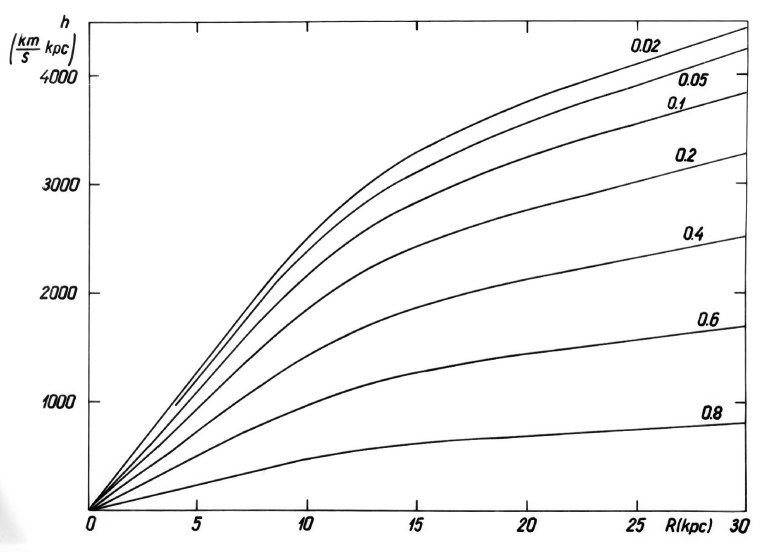
Figure 1: Angular momentum $h$ of populations of various flatness $\epsilon$ as function of the distance $R$.

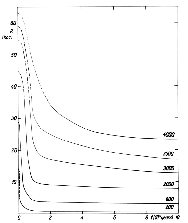
Figure 2: The evolution of the distance from galactic centre $R$ of gas clouds of various angular momentum $h$.

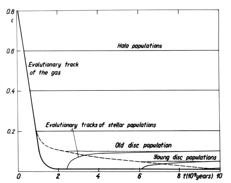
Figure 3: Possible evolution of the flatness $\epsilon$ of stellar and gas populations with time. The evolution of stellar populations is shown by thin lines, that of the gas by bold line. Evolution is shown for two cases: the bold solid line is for the case when gas immediately arrives the final $\epsilon$, the bold dashed line is the case when for $\epsilon\leq 0.2$ gas gets the flatness as given by respective present stellar population flatness.

Every line in Fig. 1 corresponds to a population of certain age, see Table LABEL:Tab7.4. According to our assumptions, stellar populations are indicators of the gas at its formation time. In this way, the Fig. 1 shows at which distance from the galactic centre, $R_{g}$, gas clouds of certain angular momentum $h$ were at respective time of the evolution $t$. Using data shown in Fig. 1, we can find the relationship between distance $R_{g}$ and time $t$ for gas clouds with given angular momentum $h$. For six values of $h$ this relationship is shown in Fig. 2.

In this way, we can reconstruct the evolution of gas population, starting from the formation of first generation of stars, using their respective specific angular momentum. Earlier evolution of gas clouds can be estimated by the extrapolation using a certain model for the initial conditions of gas clouds, and a certain regularity of the change of $R_{g}$ with time. We shall discuss this problem in the next section. In Fig. 2 extrapolated parts of curves are plotted by dashed lines.

Our results confirm and extend the evolution picture by von Hoerner (1960) and Eggen et al. (1962). In the initial phase of the evolution, the collapse of the gas was very rapid. In later phases the speed of the collapse decreased; at the present epoch the collapse has stopped completely. The collapse rate, i.e. the ratio of initial radius $R_{g}$ to the present one $R$, is very large for the nucleus of the Galaxy, and relatively modest for more distant regions.

We can use our data to reconstruct the gas evolution in the vertical direction too.

To characterise the vertical extent of populations, we shall use the flatness (axial ratio $\epsilon$) of ellipsoids of various density. In Fig. 3 we plot on vertical axis $\epsilon$, and on horizontal axis $t$ – the age of the Galaxy, counting from the formation epoch of oldest populations; the present age of the Galaxy is taken equal to 10 billion years, see Chapter 23. If we assume that dynamical and spatial parameters of populations, including flatness $\epsilon$, do not change with time, then evolutionary tracks of stellar populations in Fig. 3 are horizontal lines, starting from the point corresponding to the formation of the population. The length of these lines shows the age of the population. The solid bold line along formation points shows the evolutionary track of the gas. We see that in vertical direction, gas also has collapsed and that the collapse was very rapid in the early phase of the evolution. From flatness $\epsilon=0.2$ onwards the speed of vertical collapse decreased (dashed bold line).

This picture corresponds to the assumption that dynamical parameters of stellar populations do not change with time. In this case the collapse of the gas after rapid initial phase proceeds very slowly. Several authors, including Eggen et al. (1962), stress that the collapse was very fast, and after the collapse the gas obtained its equilibrium stage close to the present form. If we accept this assumption, then the evolutionary track of the gas from point with $\epsilon=0.20$ to point with $\epsilon=0.016$ is slowly decreasing; this section of the curve in Fig. 3 is drawn with a dashed bold line. The other possibility is that the gas obtained its present flat configuration immediately after the collapse, this variant is plotted in Fig. 3 by a solid bold line for $\epsilon<0.20$. Respective evolutionary tracks of stellar populations are drawn with thin lines. We see that in the second case the thickness of stellar populations increases with time.

Preliminary results of this study were presented by Einasto (1970a), using a slightly different calibration of ages of stellar populations. The difference between extreme populations was slightly larger than found now.

The actual evolutionary track of gas probably lies between extremal cases considered. Since some dynamical evolution of stellar populations is probable, then the lower evolutionary track of the gas is probably closer to the actual evolution. This problem was discussed by Parker (1968), see also Chapter 23.

Our conclusions on the radial and vertical collapse of the gas during the evolution of the Galaxy were based on arguments, different from arguments used by von Hoerner (1960) and Eggen et al. (1962). Our results on the fast initial collapse of the gas depend on the accuracy of determinations of ages of old halo populations. Estimates of absolute ages have a relative error about 10 %. Errors of determinations of chemical composition also increase errors. For this reason we counted ages relative to oldest halo populations, for which we used the age 10 billion years. In calculating relative ages we take into account results of modelling the evolution of stars, discussed in more detail in the next section.

4 Model of the evolution of the protogalaxy

In order to have a choice to select a model for protogalaxy evolution, we have to consider the initial conditions we can have from cosmological data.

The detection of relict radiation, chemical composition of the primeval matter and a number of other data give strong support to the primeval-fireball or “Big Bang” model of the formation of the Universe. According to this model matter and radiation were in thermodynamical equilibrium (Peebles (1965) and Doroshkevich et al. (1967)), and formed an almost homogeneous medium. There existed small density fluctuations, responsible for the formation of galaxies (Lifshitz 1946). The nature of fluctuations is not clear, they can have a whirl character, as suggested by von Weizsäcker (1951) and Ozernoi & Chernin (1967, 1968); Ozernoi & Chibisov (1970), adiabatic, as emphasised by Peebles (1965); Peebles & Yu (1970) and Silk (1968), or entropic (Doroshkevich et al. (1967), Peebles & Dicke (1968)), for review see Ozernoi (1970). For our goal, the nature of perturbations is of less interest, important is their presence.

During the evolution, the Universe expands and its density and temperature decrease. At a temperature of about 4000 K^∘ the recombination of gas starts. The matter is free from radiation, and density fluctuation can start to amplify. In this way, the density initially decreases due to the expansion of the Universe, and thereafter, the density increases in some regions due to the self-gravity of gas clouds.

To find the possible speed of the collapse, we consider a simple model, starting from the moment of the largest expansion with its turnover radius. At this epoch fluctuations of the density were still small, and we can use a model with homogeneous density, following Mestel (1963), Crampin & Hoyle (1964), and Innanen (1966b), rotating with constant angular velocity, $\omega_{0}$. We assume that at the moment when the protogalaxy had its largest extent at turnaround, it separated itself from the surrounding gas, and its mass and total angular momentum obtained their present constant values.

Present data are not sufficient to find for each protogalaxy its initial radius $R^{\circ}$ and density $\rho_{0}$. But radius $R^{\circ}$ can be found from observational data under certain assumptions. To estimate $R^{\circ}$ we can use apogalactic distances of high-velocity stars. We can assume that these distances did not change essentially during the galaxy evolution, since changes of the regular gravitational field as well relatively weak irregular forces cannot change orbits substantially. Calculations by Eggen et al. (1962) indicate that some stars have apogalactic distances of the order of $50-100$ kpc. It is clear that these values are not very accurate, since observational errors and errors in the model of the Galaxy influence results.

We can get independent estimates of $R^{\circ}$ in an indirect way, using a model of the protogalaxy with $\omega_{0}=const$. Since angular moment keeps its value during the evolution, we have

$$h=\omega\,R^{2}=\omega_{0}\,R_{0}^{2},$$ (2)

where $\omega$ and $R$ are angular velocity and distance of gas clouds at the present epoch, and $\omega_{0}$ and $R_{0}$ at the initial moment. $R_{0}$ values for various $h$ can be found from data, presented in Fig. 2. Results are given in Table LABEL:Tab21.1.

Table 1:

$h$	$R_{0}$	$\omega_{0}$
km/sec kpc	kpc	km/sec/kpc
200	$>5$	$<4$
800	28	1.0
2000	45	1.0
3000	$\geq 50$	$\geq 1.2$

We see that $\omega_{0}=1$ km/sec/kpc can be accepted. The maximal value of the angular momentum is slightly larger than 4000 km/sec kpc, which yields $R_{0}\approx 65$ kpc. This is in good agreement with the estimate from apogalactic distances.

Using this $\omega_{0}$ value we calculated for all $h$ initial radii $R_{0}$, and made extrapolation of evolutionary lines in Fig. 2 for early epochs. Using Eq. (2) we can calculate also the contraction degree of gas

$$d={R_{0}\over R}=\left({\omega\over\omega_{0}}\right)^{1/2}.$$ (3)

The initial distance $R_{0}$ and logarithm of the contraction degree $\log d$ are shown in Fig. 4 for four test populations of flatness $\epsilon=0.02,\leavevmode\nobreak\ 0.1,\leavevmode\nobreak\ 0.55,\leavevmode\nobreak\ 0.8$. As argument we use the present distance $R$.

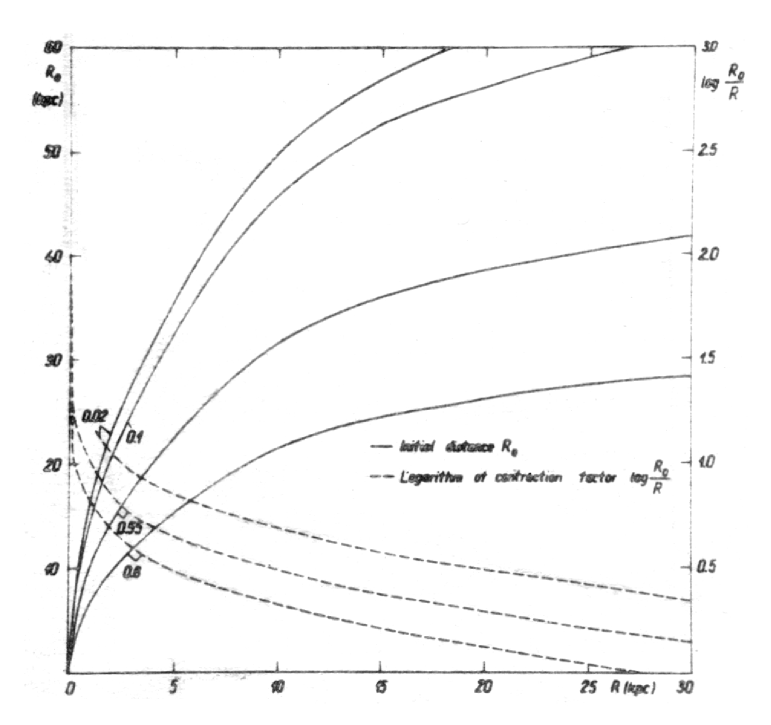
Figure 4: The initial distance, $R_{0}$ (solid lines), and contraction degree, $\log\,d$, (dashed lines) of populations with various $\epsilon$ as function of the present distance $R$.

We can use the model with constant angular momentum to estimate the contraction time. The fastest contraction has the free-fall model. This case is realised when the gas cooling time is much smaller than the free-fall time. To simplify calculations, we assume that during the contraction gas shells are not mixed, in other words, the test particle falls together with the shell it belongs to. In this case the internal mass $\mathfrak{M}\,_{int}$ remains constant. Arguments for this case were given by Crampin & Hoyle (1964).

The contraction time from initial $R_{0}$ (apogalacticum) to distance $r$ is as follows

$$t_{contr}=\sqrt{{a_{3}\over G\mathfrak{M}\,_{int}}}(\arccos x+e\sqrt{1-x^{2}}),$$ (4)

where $a$ and $e$ are major semiaxis and eccentricity of gas particle orbits, and

$$x={r-a\over ae}.$$ (5)

Major semiaxis $a$ can be found from apogalactic distance $R_{0}$, and we get

$$t_{contr}=\sqrt{{R_{0}^{3}\over G\mathfrak{M}\,_{int}}}\,f(x),$$ (6)

where

$$f(x)={1\over(1+e)^{3/2}}(\arccos x+e\sqrt{1-x^{2}}).$$ (7)

The variable $x$ can be expressed through $e$ and contraction degree $d$ as follows

$$x={1+e-d\over e\,d},$$ (8)

and the eccentricity $e$

$$1-e={h^{2}\over G\mathfrak{M}\,_{int}\,R_{0}}.$$ (9)

For the internal mass we can take

$$G\,\mathfrak{M}\,_{int}=R^{3}\omega_{c}^{2},$$ (10)

where $\omega_{c}$ is the angular velocity of circular motion. Using for $h$ the expression (2) through $R_{0}$ and $\omega_{0}$ we get

$$1-e={d^{3}\over d_{0}^{4}},$$ (11)

where $d_{0}$ is the contraction degree of objects of flat populations.

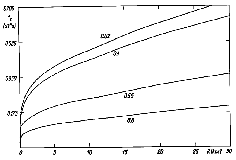
Figure 5: Contraction time of populations of various flatness $\epsilon$ as function of the distance $R$. Populations as in Fig. 4.

Since $d_{0}>d\gg 1$, then for all cases of practical interest $e\approx 1$ and $x\approx-1$, and thus $f(x)\approx 1$. This means that we can ignore the factor $f(x)$ in the contraction equation. Using Eq. (10) and expressing time in years and angular velocity in km/sec/kpc, we can write Eq. (6) as follows

$$t_{contr}={10^{9}\over\omega_{c}}d^{3/2}={10^{9}\over\omega_{c}}(\omega/\omega_{0})^{3/4}.$$ (12)

This equation was used to calculate contraction time, where $\omega(R)$ and $\omega_{c}(R)$ were taken from our model of the Galaxy. For several test populations results are given in Fig. 5. Our calculation suggest that the nucleus forms very quickly, in 10 millions years. Thereafter, new gas masses fall to the nucleus, shell after shell. In the Solar neighbourhood star formation begins about $10^{8}$ years after the condensation of the nucleus. The formation of the halo takes about one billion years. The whole process of gas contraction takes less than a billion years.

Similar calculations emphasise that the contraction of gas in vertical direction proceeds approximately with the same speed.

The model is certainly rather crude. Actually, the contraction time can be longer if the gas cools slowly. The time can be shorter if initial volume of the gas was smaller that adopted in our model. In a more accurate discussion of the problem, it must be taken into account that the gas probably consisted of many clouds moving in respect to each other. This aspect was recently studied by Brosche (1970). However, he discussed the contraction of the whole galaxy, thus, his model cannot be used to understand the differential picture.

The contraction model was discussed by Sandage et al. (1970) and Rood & Iben (1968). Sandage argued that the formation of globular clusters and other halo objects was completed in about $2\times 10^{8}$ years, whereas Rood and Iben supported a much longer formation period. When we compare data used by these authors, we see that the controversy is not real. Inner objects of the halo, studied by Eggen et al. (1962) and Sandage et al. (1970), can really be condensed quickly, but the whole process of halo forming is much longer.

Another aspect of the discussion on star formation is related with the eccentricity $e$ of stellar orbits. As discussed above, during the contractions of the protogalaxy, the eccentricity $e$ does not change much. In this case halo stars should have had large eccentricity $e$ already during their formation. In other words, gas clouds from which halo stars formed should have moved in extended elliptical orbits, which took place when the protogalaxy condensed quickly. If the gas was subject to non-gravitational forces, then objects with large eccentricity could form also in case the gas did not contract (Rood & Iben 1968). However, the influence of non-gravitational forces is strong enough only if the gas is hot, but star formation in a hot gas is impossible (Sandage et al. 1970). We conclude that the gas contraction was probably rather rapid. But here we do not have a final answer, because of the lack of a quantitative theory of star formation.

In connection with the contraction of the gas in the protogalaxy we have two additional remarks.

High-velocity hydrogen clouds were recently detected in high galactic latitudes (Dieter 1969). The origin of these clouds is not clear. But it is possible that they are remnants of protogalactic gas, which now fall towards the plane of the Galaxy. If this is the case, then the total contraction time of the protogalaxy is longer than accepted so far.

Some authors argue that spherical subsystems of the Galaxy were formed by an outburst from the nucleus or disc (Gurevich 1964), or in other words, that the star forming started only after the contraction of the protogalaxy. However, as demonstrated by Rood & Welch (1971), this hypothesis does not explain the differences in chemical composition of stars. Stars in the nucleus of the Galaxy are metal-rich, in contrast to metal-poor halo stars. In the Solar neighbourhood all stars with metal deficit have large $z$-velocities (Dixon 1965, 1966, 1967b). On the other hand, minimal heavy element content of disc stars is about half of the Solar content. All these facts suggest that the halo cannot be formed by the throw-out of stars from the nucleus or disc. Only runaway stars can be formed in this way.

5 Distribution of the angular momentum of M31

Mestel (1963) and Crampin & Hoyle (1964) found that the distribution of the angular momentum in spiral galaxies is in good agreement with the distribution of angular momentum in a homogeneous ellipsoid, rotating with constant angular velocity. Crampin & Hoyle (1964) interpreted this result as an argument favouring the formation of galaxies from a homogeneous ellipsoid of gas clouds, and that in the formation of galaxies the turbulence did not play an important role, which could redistribute the kinetic moment.

On the other hand, Lynden-Bell (1967a) noticed that all elliptical galaxies and cores of spiral galaxies are very similar, if we ignore differences in ellipticity. If we do not assume that the formation conditions of elliptical galaxies and cores of spiral galaxies were identical, we must conclude that the similarity is caused by violent relaxation during the formation of galaxies. Lynden-Bell (1967b) studied this problem in detail, and found that a fast change of the gravitation field during the contraction of the protogalaxy leads to the observed effect. This theory was checked with numerical experiments by Hohl & Campbell (1968); Hohl & Feix (1968), Cuperman et al. (1969), Henon (1969), and Goldstein et al. (1969). These experiments confirmed that the statistical method by Lynden-Ball describes well the observed energy distribution of stellar systems.

Results by Lynden-Bell suggest that during the formation of elliptical galaxies and cores of spiral galaxies the turbulence played an important role. For spiral galaxies this result is in contradiction with the Crampin & Hoyle (1964) study. In order to have an independent check, we can use our models of the Galaxy and M31 and calculate the distribution of the angular momentum. It is better to use the model of M31, since the distribution of mass in central regions of M31 is known better.

Let us assume for simplicity that surfaces of $\omega=const$ are concentric cylinders (Mestel (1963), Crampin & Hoyle (1964) and Innanen (1966b)). An essential fraction of the kinetic moment is concentrated in a thin disc, where the difference between the actual surface of $\omega=const$ and respective surface in a cylinder is small, see Chapters 7 and 20). A larger difference is expected only in the central core, where it is better to identify surfaces $\omega=const$ with surfaces $\rho=const$.

With these assumptions, the distribution of the mass as function of the kinetic moment $h$ is the following (Mestel (1963) and Crampin & Hoyle (1964))

$$m(h)=\mathcal{P}\,[R(h)]\,\frac{{\rm d}R\,}{{\rm d}h\,},$$ (13)

where

$$\mathcal{P}\,(R)=2\pi\,R\,P(R)$$ (14)

is the mass of cylindric shell of unit thickness, and $P(R)$ is the projected density. Further we have

$$\frac{{\rm d}h\,}{{\rm d}R\,}=R\left(\frac{V_{\theta}}{R}+\frac{{\rm d}V_{\theta}\,}{{\rm d}R\,}\right).$$ (15)

Here we can accept the approximation

$$V_{\theta}=\beta\,V,$$ (16)

where $V$ is the circular velocity. Applying Oort dynamical parameters $A,\leavevmode\nobreak\ B$ and using $k_{\theta}=-B/(A-B)$, we get

$$\frac{{\rm d}R\,}{{\rm d}h\,}=\frac{1}{2k_{\theta}}\,\frac{R}{h}.$$ (17)

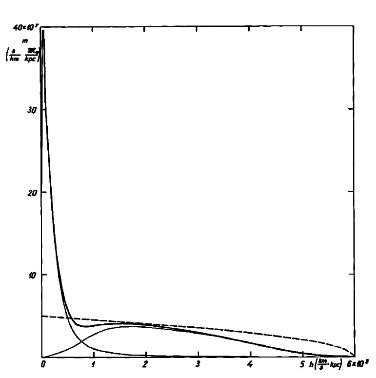
Figure 6: The mass distribution of M31 as function of the angular momentum $h$ (solid line). Dashed line shows a similar distribution of a body rotating with constant angular speed.

The distribution of the mass as function of $h$ using Eq. (13) and (17) is shown in Fig. 6. The bold curve shows the total distribution, thin curves show the distribution for the first and second population. To the first population we include the disc and flat components, for them we used the value $\beta=0$ on the basis of results from Chapters 4 and 7. The second population includes the core (using data from Chapter 20 we accepted $\beta=0.4$) and the halo. The halo was divided into two components of different mass with values of the parameter $\beta=0.3$ and $\beta=0.6$. We see that the distribution of the momentum of the first and second population are very different.

Mestel (1963) and Crampin & Hoyle (1964) compared distributions of the mass vs. kinetic moment of galaxies with similar distributions for homogeneous spheroids, rotating with constant angular velocity. For this distribution, we have

$$m(x)=3/2\,\mathfrak{M}\,\sqrt{1-x},$$ (18)

where $\mathfrak{M}\,$ is the mass of the spheroid, and

$$x=h/h^{0},$$ (19)

where $h^{0}$ is the maximal kinetic moment at the periphery of the model. The mass of the M31 model is known, and we get for the maximal moment using data from Fig. 6: $h^{0}=6000$ km/sec per kpc. This function is also plotted in Fig. 6.

We see that the homogeneous model describes the function $m(h)$ only in very general terms. In the periphery of the galaxy the function $m(h)$ approaches zero more slowly than the homogeneous model. This suggests that the protogalaxy did not have a sharp outer boundary, i.e. the density approached smoothly zero. Another difference between models is observed near the centre of the system, where the model has essential deficit of mass with low kinetic moment. This difference can be due to the presence of a dense nucleus in the protogalaxy. However, a more likely explanation of the mass excess with small angular momentum is the redistribution of moment during the fast contraction of the protogalaxy. The distribution of the moment is in agreement with the Lynden-Bell hypothesis on the violent redistribution of matter during the formation of the protogalaxy.

However, we note that the violent relaxation happens only in the central region of the Galaxy. This factor cannot strongly change our picture on the general evolution of the protogalaxy.

September 1971

Chapter 23 Physical evolution of stellar systems

1 Introduction

For the full description of the structure of galaxies and other stellar systems it is necessary, in addition to kinematical and spatial description functions, add also functions which describe the physical structure of galaxies and their populations. Such functions include the distribution of various spectral characteristics, chemical content, age and other similar quantities. During the evolution of galaxies these functions change with time.

The change of physical characteristics of galaxies with time is caused by the dynamical evolution of galaxies (redistribution of mass), and by the change of physical characteristics of stars due to stellar evolution. Advances in our understanding of stellar evolution permit to follow the physical evolution of galaxies, and to build models of the evolution of stars and gas in galaxies. Pioneering studies in this direction were made by Limber (1960) and Tinsley (1968). In this Chapter, we describe our model of the physical evolution of galaxies. To construct the model, we need to know the rate of star formation, evolutionary tracks of stars of various masses in the Herzsprung-Russell diagram, and bolometric data and colours of stars as functions of the effective temperature and bolometric luminosity.

2 Data and method

1 Initial mass function of stars

The initial distribution of stars according to their mass and luminosity and the division of stars into giants and main-sequence stars was discussed already by Öpik (1938). Using modern data, the luminosity function and stellar evolution was discussed by Salpeter (1955). He found that the number of stars of mass $M$, $F(M)$, formed in unit time interval per cubic parsec, can be expressed by the following equation,

$$F(M)=a\times M^{-n},$$ (1)

where $a$ and $n=2.35$ are constants. In the derivation of this equation Salpeter assumed that the rate of star formation is constant during the last $5\times 10^{9}$ years and that stars move from main sequence stars to giants when they have consumed 10 % of their hydrogen.

This result was confirmed by Sandage (1957a) and van den Bergh (1957) and other authors, using counts of stars in young star clusters. Later it was understood that the rate of star formation is not constant but changes in time, see below. However, this does not change the form of Eq. (1). In an overview, Reddish (1966) concluded that the equation (1) with exponent $n=2.5$ can be used in the interval of stellar masses $M_{0}\leq M\leq M_{u}$, where $M_{0}$ and $M_{u}$ are minimal and maximal masses of forming stars. For medium mass stars observational data are better represented using Eq.  (1) with $n=2.33$. The total mass of forming stars is equal to

$$\int_{M_{0}}^{M_{u}}F(M)M\,{\rm d}M\,.$$ (2)

We cannot use for the minimal mass a value $M_{0}=0$, since the integral Eq. (2) is not converging in this case. It is possible that the function $F(M)M$ smoothly approaches zero when $M\Rightarrow 0$. Our results do not depend on the exact form of the function $F(M)$ for small $M$. For this reason, we take $M_{0}$ as the effective lower limit of mass of forming stars and take $F(M)=0$, if $M<M_{0}$. In solar neighbourhood of the Galaxy, we can use $M_{0}=0.03$ in solar units (Reddish 1966).

According to Reddish (1966), there exists an upper limit of mass of forming stars, $M_{u}=60-100\leavevmode\nobreak\ M_{\odot}$. A similar upper limit is predicted by theory. Stothers & Simon (1968) demonstrated that blue supergiant stars are unstable for pulsations when they have masses in excess of 65 $M_{\odot}$. However, as shown by Talbot (1971), stars cross the instability zone very fast and cannot lose their mass during this period very much. For this reason, we take as the upper limit of forming stars $100\,M_{\odot}$, not $65\,M_{\odot}$. We chose the parameter $a$ in Eq.  (1) from the condition that the integral Eq. (2) is equal to unity. In this case we get

$$a=(n-2)(M_{0}^{2-n}-M_{u}^{2-n})^{-1}.$$ (3)

The choice of parameters $M_{0}$, $M_{u}$ and $n$ is crucial in the modeling the physical evolution of galaxies. Earlier it was assumed that these parameters are constants. However, already Limber (1960) demonstrated that in this case it is impossible to explain differences in mass-to-light ratios of globular clusters ($f_{V}=\mathfrak{M}\,/L_{V}\approx 1$), dwarf galaxies ($f_{V}\approx 10$), and giant elliptical galaxies ($f_{V}\approx 100$), all having approximately similar ages.

Differences in the parameters of star formation function can probably be explained by differences in the chemical composition of old stellar populations of galaxies. van den Bergh (1961) hinted to the fact that the fraction of heavy chemical elements is different in globular clusters and in old open clusters, both having approximately equal ages. Heavy elements are synthesised in stars. Rapid enrichment of interstellar gas by heavy elements is done by massive stars with fast evolution. The large variability of chemical compositions of stars of different old populations suggests that in the early period of the evolution, various populations had different fractions of massive stars, much higher than the present fraction of massive stars. This conclusion was made by Schmidt (1963), Truran & Cameron (1970) and Cameron & Truran (1971).

Such effects can be explained if we assume that the minimal mass of forming stars, $M_{0}$, depends on time, or more accurately, on the fraction of heavy elements in the interstellar gas during the formation of stars of different populations. Truran & Cameron (1970) suggested a mechanism to explain these differences.

2 Star formation rate

Salpeter (1955) assumed that the star formation rate in the Galaxy is approximately constant. More accurate data showed that in the early phase of the evolution of the Galaxy, the star formation rate was considerably higher (von Hoerner 1960). In the early phase of the evolution of the Galaxy, the density of interstellar matter was much higher than in the present epoch. Based on this argument, Schmidt (1959) concluded that the star formation rate depends on the density of interstellar matter.

We define the local star formation rate as the time derivation of the density of stars. Following Schmidt (1959) we assume that the star formation rate is proportional to the density of gas in power $S$:

$$R_{l}={{\rm d}\rho_{s}\,\over{\rm d}t\,}=\gamma\rho_{g}^{S},$$ (4)

where $\rho_{s}$ and $\rho_{g}$ are star and gas densities, respectively, and $\gamma$ and $S$ are constants. We assume that the full matter density in a volume element, $\rho=\rho_{s}+\rho_{g}$, does not depend on time. In this case after integration of Eq. (4) we get

$$\rho_{g}=\rho[1+(S-1)\tau]^{-1\over S-1},$$ (5)

where

$$\tau=t/K,$$ (6)

and for the characteristic time $K$ we have

$$K=(\gamma\rho^{S-1})^{-1}.$$ (7)

In case $S=1$ we get

$$\rho_{g}=\rho\,e^{-\tau}$$ (8)

and

$$K=\gamma^{-1}.$$ (9)

Integrating Eq. (4) over the whole volume of the stellar system, and assuming that the gas amount does not depend on time, we get for the whole gas mass

$$\mathfrak{M}\,_{g}=\mathfrak{M}\,[1+(S-1)\tau]^{-1\over S-1},$$ (10)

where $\mathfrak{M}\,=\mathfrak{M}\,_{s}+\mathfrak{M}\,_{g}$ is the full mass of the galaxy, and $\mathfrak{M}\,_{s}$ is its stellar mass. For the characteristic time we get

$$K=(\gamma\bar{\rho}^{S-1})^{-1},$$ (11)

where $\bar{\rho}=\mathfrak{M}\,/V_{\ast}$. Here $V_{\ast}$ is the mean volume of the gas, which can be calculated as follows:

$$V_{\ast}^{-(S-1)}=\mathfrak{M}\,_{g}^{-s}\int\rho_{g}^{S-1}{\rm d}\mathfrak{M}\,_{g}\,.$$ (12)

In particular case $S=1$ we get

$$\mathfrak{M}\,_{g}=\mathfrak{M}\,\,e^{-\tau}.$$ (13)

The characteristic time $K$ is the essential parameter which describes the star formation rate in galaxies. The characteristic time depends on the parameter $S$. If $S=0$, then the star formation rate is lower for higher mass density; if $S=1$, then the characteristic time $K$ is constant; if $S=2$, then the star formation rate is the higher, the higher is the matter density. Observational data on the density and mass of stars and gas suggest that $S=2$. This conclusion has been made by Schmidt (1959) and Sanduleak (1969). However, we shall make calculations for all values, $S=0,\leavevmode\nobreak\ 1,\leavevmode\nobreak\ 2$. It is easy to show that if $K\Rightarrow\infty$ then all variants lead to $S=0$.

3 Evolutionary tracks of stars

Presently several series of calculations of stellar evolutionary tracks are available. The most used series of evolutionary tracks was calculated by Iben (1965a, b, 1966a, 1966c, 1966b, 1967c, 1967a). For this series, the following chemical abundance was used: $X=0.71$, $Y=0.27$ and $Z=0.02$; models were calculated for stellar masses: $0.5,\leavevmode\nobreak\ 1.0,\leavevmode\nobreak\ 1.25,\leavevmode\nobreak\ 1.5,\leavevmode\nobreak\ 2.25,\leavevmode\nobreak\ 3,\leavevmode\nobreak\ 5,\leavevmode\nobreak\ 9,\leavevmode\nobreak\ 15\,M_{\odot}$. In another series, Iben with collaborators calculated models of population II metal-poor stars: Faulkner & Iben (1966), Iben & Faulkner (1968), Rood & Iben (1968), Iben (1968), Iben & Rood (1970a), Rood (1970), Iben & Rood (1970b), Simoda & Iben (1970) and Iben (1971). Chemical abundance parameters $X,\leavevmode\nobreak\ Y,\leavevmode\nobreak\ Z$ were varied, most models were calculated for initial stellar masses around the solar mass. Another similar series of models was calculated by Demarque (1967), Demarque et al. (1968), Demarque & Schlesinger (1969), Demarque & Miller (1969), Demarque et al. (1971), and Demarque & Mengel (1971a, b). Recently a series of evolution models was calculated by Paczyński & Ziółkowski (1968) and Paczyński (1970a, b, c, 1971), who accepted abundance parameters $X=0.70$, $Y=0.27$ and $Z=0.03$, calculations were made for stellar masses $0.8,\leavevmode\nobreak\ 1.5,\leavevmode\nobreak\ 3,\leavevmode\nobreak\ 5,\leavevmode\nobreak\ 7,\leavevmode\nobreak\ 10,\leavevmode\nobreak\ 15\,M_{\odot}$.

Table 1: Evolutionary tracks

In this work, we are mainly interested in the evolution of stars with normal chemical abundance with $Z=0.02-0.03$. Models by Iben and Paczynski are slightly different. Paczynski calculated models until the carbon ignition for massive stars, and until helium ignition for less massive stars. As a rule, Iben’s models were not calculated until these late evolution phases. On the other hand, Iben has calculated more models for stars of low mass. For the present work just the evolution of low-mass stars is important. Taking all these arguments into account we selected Iben’s models as the basis for our use and used Paczynski models for late evolutionary phases of stars. For very massive stars ($M=30,\leavevmode\nobreak\ 60\,M_{\odot}$), we used models by Stothers (1963a, 1964, 1966) and Stothers & Chin (1968, 1969). For stars of very small mass, we used models calculated by various authors: Kumar (1963b, a), Hayashi & Nakano (1963), Rose & Smith (1970), Grossman (1970); Grossman et al. (1970); Grossman & Graboske (1971).

Tracks used in this paper are given in Table 1. We tabulated evolutionary tracks for stars of mass: 0.05, 0.1, 0.2,  0.4,  0.6,  0.8,  1.0,  1.25,  1.5,  2.25,  3,  5,  9,  15,  30,  $60\,M_{\odot}$. In all tracks 19 points were given, each point corresponds to a certain stage in the evolution of stars, for comparison see Fig. 3 by Iben (1967b). In our table point 3 corresponds to the arrival of star to the “zero-age” point on the main sequence, point 13 corresponds to the maximum temperature in the helium burning phase, point 16 to the tip of red giants (carbon ignition for massive stars), point 18 to the beginning of the white dwarf sequence, point 19 to the arrival of star to the cold red region. In most cases, data were taken directly from respective papers, in some cases interpolation and combination from various sources was needed. Below we give some details on the interpolation and combination of published evolutionary tracks.

A. Gravitational contraction phase. The time spent on the gravitational contraction phase was calculated for stars of small mass using data by Kumar (1963b). For massive stars, the contraction time was estimated by extrapolation in Iben’s models.

B. Core hydrogen burning. Most data on tracks were taken directly from published sources. The track for mass $0.8\leavevmode\nobreak\ M_{\odot}$ was found by interpolating tracks by Iben for mass 1 and $1.25\leavevmode\nobreak\ M_{\odot}$, and track for $0.8\leavevmode\nobreak\ M_{\odot}$ by Paczynski. The time was estimated as follows:

$$\log\,t_{0.02}=\log\,t_{0.03}+\Delta,$$ (14)

where $t_{0.03}$ is the time according to the respective model by Paczynski, and $\Delta=0.112$ is a correction, calculated as follows. The time spent to burn $\Delta\,M$ solar mass of hydrogen by a star of luminosity $L$ is equal to $\tau_{H}\propto\Delta\,M/L$. Most of this time the star is located on the main sequence. In the range of stellar masses of interest $L\propto M^{4}$. If we suppose that in all stars the same fraction of mass is burned, then $\tau_{H}=a\,M^{-3}$, where $a$ is a certain constant. Relations given above have an approximate character, and we get

$$\tau_{H}\,M^{3}=a(M),$$ (15)

where $a(M)$ is a slow function of mass and abundance. We found this function using Paczynski models of $Z=0.03$ in the mass range $0.8\leq M\leq 3$, and using Iben models with $Z=0.02$ in the mass range $1\leq M\leq 3$. The correction $\Delta$ was estimated by the extrapolation of the $Z=0.02$ curve toward stars of smaller mass.

C. Helium burning phase. The initial phase of helium burning is well studied. The last phase of helium burning is less known. The best data come from the Paczynski series. Iben models were calculated only to early phases of helium burning. To find late phases of helium burning of Iben models, an extrapolation method is needed. This can be done using evolutionary tracks by Paczynski.

Calculations by Paczynski and others suggest that evolutionary tracks of the last phases are just continuing tracks, found for earlier epochs in the last phases of hydrogen burning in the giant branch. Uus (1970) and Paczyński (1971) showed that the speed of the growth of star luminosity in the giant branch is almost independent of the mass of stars. Hydrogen and helium ignition on this stage occurs at almost identical luminosity (Hayashi et al. 1962; Paczyński 1970a). Authors found that for $Z=0.03$ helium and hydrogen flashes occur at $\log\,(L/L_{\odot})=3.10$ and $\log\,(L/L_{\odot})=5.0$, respectively. Using these data and tracks found by Iben for early stages on giant branch, it was possible to continue tracks for later stages up to the tip of the red giant branch.

It was more difficult to estimate the time spent on helium burning stage, since most Iben tracks were calculated only for the early stages of helium burning. The most advanced track was found for the star of mass 15 $M_{\odot}$ (Iben 1966b). To continue the track, only a short last stage of evolution must be added. According to Uus (1970) and Paczyński (1971) this stage is very short, thus an error in the estimate of the time plays little role. The time spent in helium burning, $\tau_{He}$, can be compared with the time spent in hydrogen burning, $\tau_{H}$. For a star of mass $M=15\,M_{\odot}$ we get

$$\left({\tau_{H}\over\tau_{He}}\right)_{002}=\left({\tau_{H}\over\tau_{He}}\right)_{003}.$$ (16)

Paczyński (1971) showed that for $Z=0.03$ and $M\geq 3\,M_{\odot}$ the following relation exists

$$\log\,{\tau_{H}\over\tau_{He}}=-0.174+0.633\,\log\,M+0.182\,(\log\,M)^{2}.$$ (17)

The time $\tau_{He}$ for $Z=0.02$ and $M\geq 3\,M_{\odot}$ was found using Eq. (16) and (17).

If we apply these equations for stars of smaller masses, then the time $\tau_{He}$ is too large. On the other hand, Iben & Rood (1970b) showed that stars of approximate solar mass have $\tau_{He}\approx 12\times 10^{7}$ years, almost independently of the chemical composition. For $M=3\,M_{\odot}$ stars we found $\tau_{He}=1.71\times 10^{7}$ years. Since $\tau_{He}\ll\tau_{H}$, then high accuracy of $\tau_{He}$ plays little role, and we accepted for stars of mass $M\leq 3\,M_{\odot}$ $\tau_{He}=17.1\times 10^{7}$ years.

Evolutionary tracks of stars of mass $M<3\,M_{\odot}$ were calculated by Iben before the helium ignition. Thus, the whole red giant branch of the evolution during the helium burning must be estimated from other data. We used for stars of mass $0.8\,M_{\odot}$ the blue end of the horizontal branch at point $\log\,L/L_{\odot}=1.60$ and $\log\,T_{e}=3.68$. For tracks of stars of other masses, we used observational data of colour-magnitude diagrams of old star clusters by Sandage (1962), Eggen & Sandage (1964), and Newell et al. (1969).

D. Last stages of stellar evolution. Available data suggest that the final evolutionary stage of all stars is the degenerate white dwarf. The path toward this stage can be different. Very low mass stars of mass, $M\leq 0.08\,M_{\odot}$, and normal metal abundance come to this stage of “black” dwarfs directly after the initial gravitational contraction. The radius of such stars depends on its mass and chemical abundance, the star in this stage uses its thermal energy. According to Schwarzschild (1958) the time spent in this stage is

$$\log\,\tau=b+5/8\,\log\,(M/L),$$ (18)

where $b$ is a constant, depending on the chemical composition, and $M$ and $L$ are expressed in solar units. Using data by Schwarzschild (1958) we found that for red dwarfs of normal composition $b=7.42$, if $\tau$ is expressed in years.

After the formation of carbon nucleus, stars of mass $M>1.4\,M\odot$ explode as supernovae, and their nuclei become pulsars. Stars of lower mass move after the exhausting of nuclear energy through the planetary nebulae stage to white dwarfs. Due to mass loss during the evolution, the limiting mass of stars at the stage where evolutionary paths diverge, is higher than $1.4\,M_{\odot}$. According to Jones (1970), the initial mass of white dwarfs of Hyades is larger than $1.8\,M_{\odot}$. Using novae statistics by Payne-Gaposhkin (1957), Stothers (1963b) concluded that the limiting mass of stars to go through the supernova stage is $4\,M_{\odot}$. Now we shall find the limiting mass using more recent data.

According to Tammann (1970), the frequency of supernova explosions in galaxies of type Sb is 0.09 for 100 years for mass unit $10^{10}\,M_{\odot}$. This statistics is based on galaxy models by Roberts (1969a), who used Brandt (1960) mass distribution profile. As shown by Einasto (1969a), this mass distribution model yields too high masses for galaxies. For this reason, we use for the Galaxy a mass $M=15\times 10^{10}\,M_{\odot}$, and get the frequency 1 supernova per 74 years. This frequency is in good agreement with the estimate by Caswell (1970) (40–80 years), based on radioastronomical data on the frequency of supernova remnants in Galaxy. Using star formation function Eqs. (1) and (3) with parameters $n=7/3$, $M_{0}=0.03\,M_{\odot}$ and $M_{u}=100\,M_{\odot}$, and for the speed parameter of star formation in Eq. (11) $K=0.25\times 10^{9}$ years, we find that in our Galaxy in the present epoch 3.5 stars form per year. The frequency 1 supernova per 74 years corresponds to the lower bound of mass of supernova progenitor stars: $2.6\,M_{\odot}$. We accept this value for further calculations. Optical luminosity of supernova remnants (pulsars) decreases very fast, and they are practically optically invisible (Pacini 1971). Their luminosity is not known. In our calculation we used for their luminosity the value $\log\,L/L_{\odot}=-9.$

Let us now discuss the last evolutionary stages of stars of intermediate mass. According to Paczyński (1970a) the luminosity of stars during the path towards nuclei of planetary nebulae depends only on the mass of the nucleus of the star $M_{c}$ (the future white dwarf):

$$L/L_{\odot}=59\,250\,M_{c}/M_{\odot}-30\,950.$$ (19)

It follows from the same data that the mass of the nucleus depends on the initial mass of stars. Interpolating Paczyński (1970a) data we get for stars of initial masses 2.25, 1.25 and 1 $M_{\odot}$ masses of nuclei 1.0, 0.7 and 0.65 $M_{\odot}$, respectively. The time spent on these evolutionary stages was taken from Table 2 of Paczyński (1970a).

Evolutionary tracks for white dwarfs were taken from Schwarzschild (1958). We used data from Table 28 of Schwarzschild (1958), the time spent in this stage was calculated using Eq, (18), where we used for the parameter $b$ a value $b=7.05$. This equation is evidently approximate. In the last stage of their evolution, white dwarfs start to crystallise (van Horn 1968), which initially slows the cooling but later speeds it. These details play practically no role in the determination of integral characteristics of galaxies and can be ignored. In our calculations we used as the last point of the evolutionary track of white dwarfs $\log\,L/L_{\odot}=-4.6$. The total time spent by stars to reach this point exceeds 20 billion years, independent of the mass of stars. This was the maximal epoch used in calculations of stellar evolutionary tracks.

Table 2: Intrinsic colours and bolometric corrections

4 Bolometric corrections and colour indexes

Theoretical evolutionary tracks are given in coordinates $\log\,T_{e},\leavevmode\nobreak\ \log\,L/L_{\odot}$, observational data are given as colours and absolute magnitudes, $B-V,\leavevmode\nobreak\ M_{V}$. To find the relationship between these data as well as to calculate mass-to-light ratios of populations and the energy distribution in spectra of model galaxies, we need to know bolometric corrections, $BC=M_{b}-M_{V}$, and intrinsic colours, $(S-V)_{0}$, of stars of all types. In the last equation $S$ denotes the star magnitude in whatever colour in the magnitude system UBVRIJKL by Johnson (1964).

As the main source of bolometric corrections, intrinsic colours and effective temperatures we used the compilation by Johnson (1966a). Also, we used some more recent sources which complement Johnson data in the infrared and ultraviolet range of the spectrum.

Johnson (1966a) published $BC$, $(S-V)_{0}$ and $T_{e}$ as functions of spectral type and luminosity class. For our purpose we need these data as functions of $\log\,T_{e}$ and $\log\,L/L_{\odot}$. We found a respective relation by graphical interpolation. As the first step we found the dependence of $\log\,T_{e}$ on spectral type, separately for the main sequence (luminosity class V), giants (III) and supergiants (I). Next we made graphs of $BC$ and $(S-V)_{0}$ as functions of $\log\,T_{e}$. Instead of intrinsic colours we used bolometric corrections in the $S$ system

$$BC_{S}=M_{b}-M_{S}=BC_{V}-(S-V)_{0}.$$ (20)

Results of calculations are given in Table 2. We give a logarithm of the luminosity in ergs for a star of zero magnitude in the UBVRIJKL Johnson (1966a) system, and the intrinsic colour of the Sun according to Mendoza (1968). Data in this Table need some comments.

Intrinsic colours. Most intrinsic colours were taken from Johnson (1966a). Data for colours $(U-V)_{0}$ and $(B-V)_{0}$ were taken from a more recent study by Fitzgerald (1970). For red stars we used the catalogue by Mendoza (1968) and data by Greenstein et al. (1970). For A and F stars of the main sequence we used data by Davis & Webb (1970).

Bolometric corrections and effective temperatures. The effective temperature of a star is defined as the temperature of the black body, which emits from the unit surface area the same amount of energy as the star. To find effective temperatures of stars, their angular sizes and bolometric luminosities are needed. Bolometric luminosities can be calculated by integrating the spectral energy distribution over wavelengths, expressed in absolute units. Angular diameters can be found from interferometric observations. When Johnson made his summary, diameters were available only for 14 stars, including Sun. Mendoza (1968) used angular diameters of 27 stars. These data were not sufficient to find the scale of effective temperatures, thus results from theoretical calculations of models of stellar atmospheres were also used.

The scale of effective temperatures and bolometric corrections for spectral classes O5–G2 was determined by Morton & Adams (1968), using model atmosphere calculations. We used these data for the main sequence stars earlier than F2 type. For stars of type F2–G2, corrections from radiometric observations were determined. The zero point of theoretical BC was chosen in such a way that at spectral type F2 theoretical model data coincide with observational data.

Recently van Citters & Morton (1970) suggested that it is better to connect BC directly with bolometric data on the Sun, BC${}_{\odot}=-0.07$. For this reason, we used for B0.5–B6 stars BC directly from van Citters & Morton (1970), for O5–B0.5 stars from Morton (1969), and for B8–F stars from Davis & Webb (1970), who used the same method to determine BC.

For effective temperatures of B0.5–B7 stars, we used the scale by Morton & Adams (1968), as this scale coincides with the scale found from angular diameters by Hanbury Brown et al. (1967) and van Citters & Morton (1970). For very bright blue stars of type O5– B0.5 Morton (1969) determined a new temperature scale, which is favoured over the theoretical scale. However, Peterson & Scholz (1971) determined effective temperatures of six stars of type O5–09.5, and found that they are higher than temperatures by Morton (1969). We shall use the temperature scale by Peterson & Scholz (1971), and to find BC we use the relationship between $T_{e}$ and BC, found by Morton (1969).

For late M dwarfs we used $T_{e}$ and BC from the paper by Greenstein et al. (1970). For red giants of type M0–M6 we used for $T_{e}$ and BC data by Lee (1970). For M7–M8 giants bolometric corrections were taken from Smak (1966a). For most red giants we determined the temperature scale, applying procedures given by Johnson (1966a). The scale of effective temperatures was based on angular diameters, given in Table V of Johnson (1966a) and in Table 2 of Mendoza (1968). Temperatures were calculated with the black-body fit method, using data given in Tables VI and VII of Johnson (1966a).

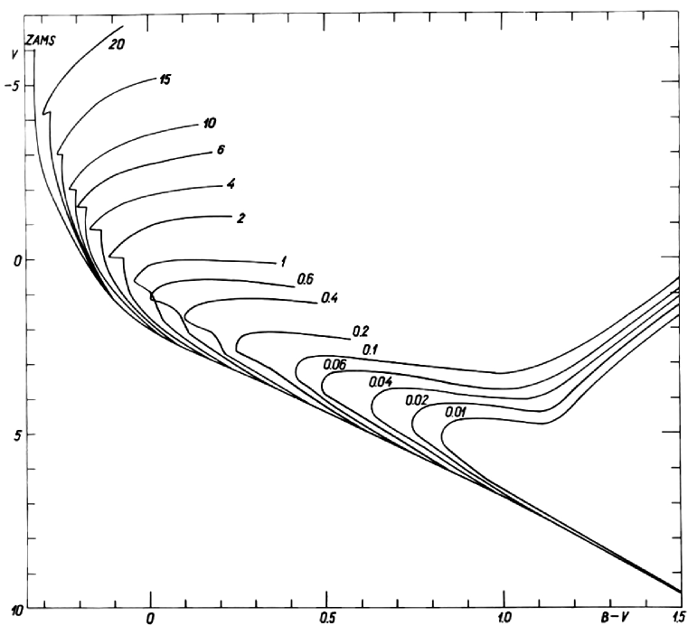
Figure 1: Isochrones of stars of normal chemical composition $Z=0.02$. Masses of stars are labeled 20, 15, 10 etc.

5 Isochrones

The collected information was used to derive isochrones of stars of various masses in the model colour-luminosity $(B-V,M_{V})$ diagram, and to study the physical evolution of stellar systems. In this section we discuss isochrones found, presented in Fig. 1. For comparison we show in Fig. 4 below colour-magnitude diagrams for selected star clusters.

We show in the Figure isochrones for the main phase of hydrogen burning of stellar evolution. We also constructed isochrones for late stages of stellar evolution, corresponding to helium burning, white dwarfs, and final stages of red “white” stars. In these late stages isochrones cross each other several times. To avoid overcrowding of the Figure these late stages are not shown.

Close to the hydrogen burning main sequence evolutionary tracks also cross. This effect was detected by Sandage & Eggen (1969) from theoretical models and later from empirical data. Around the turn-off point of the main sequence isochrones have a zigzag form. This feature was confirmed by observational data by van den Heuvel (1969), see also Iben (1967b).

In the red giant region, our compiled data agree well with data by Schlesinger (1969b). However, in a later paper Schlesinger (1969a) showed that, in contrast to observations, the helium sequence, found by Iben (1966a), extends too far toward the blue region. Schlesinger (1969a) modified his program and found for the blue tip of the helium main sequence for $M=5\,M_{\odot}$ star a value $\log\,T_{e}=3.68$, whereas according to Iben (1966a) it is $\log\,T_{e}=3.92$. The need to correct Iben’s data is confirmed by our calculations, which show that integral colours of model galaxies become too blue. For this reason, we applied for the blue end of the helium sequence of $M=5\,M_{\odot}$ stars the value $\log\,T_{e}=3.68$ by Schlesinger (1969a).

Observational data by Cannon (1970) suggest that stars of lower mass have a horizontal sequence, which is usually identified with the helium burning phase of the giant branch. It is not easy to determine the blue end of the horizontal sequence for more massive stars. In this stage both hydrogen and helium burning phases are closely located. We accepted the more extreme case, and identified the yellow and red sequences of giant stars with the helium burning phase. According to Wildey (1964) the colour of these red giants is redder than $B-V=1.00$, which corresponds to $\log\,T_{e}=3.68$. We accepted this temperature value for the blue end of the helium sequence of all stars of mass $M\geq 5\,M_{\odot}$.

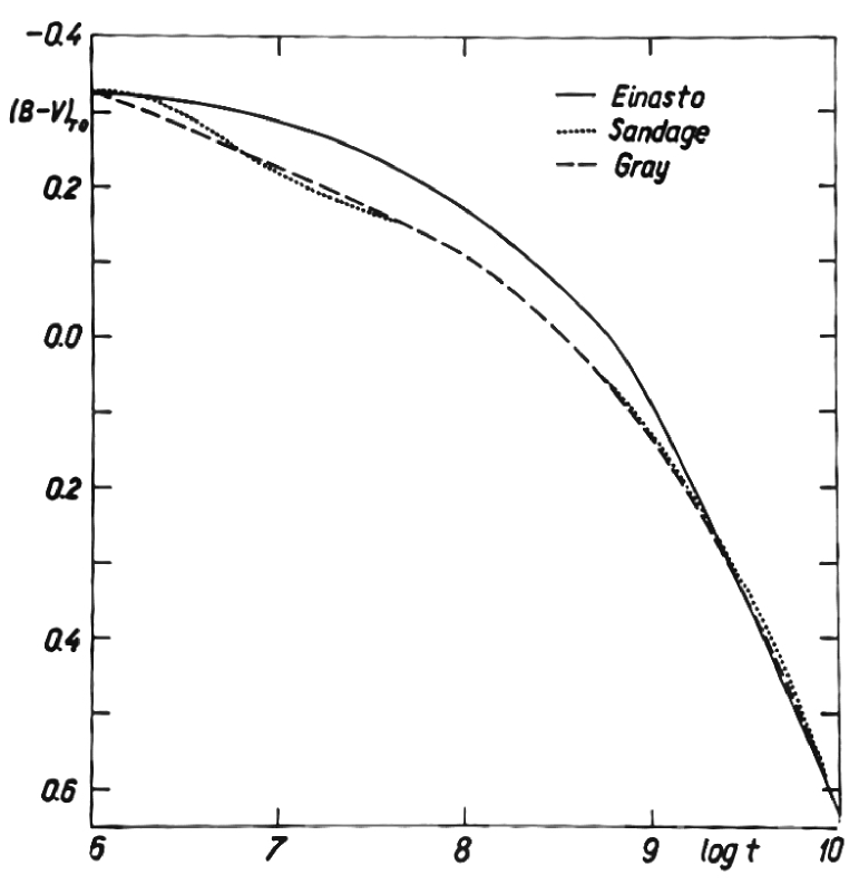
Figure 2: Colours of the main sequence turn-off point as functions of the star age according to the present paper, Sandage (1963) and Gray (1965).

The colour of the turn-off point of the main sequence is often used as the criterion of the cluster age. Using our model isochrones we made a new calibration of this relationship, results are given in Fig 2. For comparison we show here also calibrations according to Sandage (1963) and Gray (1965).

3 Time evolution of physical characteristics of model galaxies

We made calculations to follow changes in physical characteristics of model galaxies for a series of initial data. Below we describe initial data used and results obtained.

1 Initial data

Most calculations were done using following initial data for star formation rate: $n=7/3$, $M_{0}=0.03\,M_{\odot}$, $M_{u}=100\,M_{\odot}$, $S=0$  ($K=20$),  $S=1$  ($K=0.5,\leavevmode\nobreak\ 3$),  $S=2$  ($K=0.3$); here the characteristic time of galaxy formation $K$ is expressed in billion years. We calculated model galaxies for ages 0.01, 0.03, 0.3. 1, 2, 4, 6, 8, 9, 10, 15, and 20 billion years.

To find the dependence of physical properties of galaxies on the values of star formation function parameters, we made calculations for a range of $S$ and $K$, using $n=2.05$ instead of $n=7/3$. Some calculations were made using a shifted blue end of the helium burning sequence, as discussed above.

The upper limit of the star formation function, $M_{u}$, has little influence on integral properties of galaxies. The change of the lower mass limit, $M_{0}$, has little influence on colour and spectral energy distribution, but has a large impact to the luminosity, $L$, and mass-to-light relation, $f=M/L$, through the parameter $a$, see Eq. (3). The luminosity of the model galaxy and its mass-to-light ratio can be find as follows:

$$L=L_{0}/\delta,\leavevmode\nobreak\ \leavevmode\nobreak\ \leavevmode\nobreak\ \leavevmode\nobreak\ f=\delta\,f_{0},$$ (21)

where $L_{0}$ and $f_{0}$ are values of these parameters for lower mass limit $M_{0}=0.03\,M_{\odot}$. We give in Table LABEL:Tab22.3 coefficients $\delta$ and $\Delta\,M=2.5\,\log\,\delta$ for a series of minimal masses of star formation function, $M_{0}$.

Table 3:

$M_{0}$	$\delta$	$\Delta\,M$
0.50	0.348	-1.145
0.30	0.426	-0.928
0.10	0.644	-0.478
0.03	1.000	0.000
0.01	1.473	0.420
0.003	2.234	0.873
0.001	3.256	1.283

Mass-to-light ratios of old stellar populations differ considerably. According to Schwarzschild & Bernstein (1955) globular clusters have $f=M/L\approx 1$, for giant elliptical galaxies Page (1967) found values up to $f=M/L\approx 100$. Tinsley (1968) explained the large variance of $f$ in old populations with the large quantity of stars of low mass in giant elliptical galaxies. If we accept these high values of $f$, we have to use for the lower end mass of star formation function values like $M_{0}\approx 10^{-6}\,M_{\odot}$, which seem to be improbably low. If we change $M_{0}$ within the range given in Table LABEL:Tab22.3, it is impossible to change mass-to-light in such large limits. The change of the parameter $n$ in star formation rate function cannot yield so large changes in $f$ either. Tinsley & Spinrad (1971) demonstrated in the case of M31 that this parameter can be changed only in a very limited range.

On the other hand, it is well known that evolutionary tracks of stars of different chemical composition are different, which also changes integral characteristics of stellar systems. In the present time, there exists no complete series of evolutionary tracks for extremal chemical compositions. Moreover, for such stars there are no reliable bolometric corrections and intrinsic colours. However, to get an idea what possible changes of integral characteristics of galaxies and stellar populations are expected for extreme chemical compositions, we made calculations with the same program as before, but with shifted evolutionary tracks.

To get tracks for population rich in heavy elements we added to tracks, calculated for composition $Z=0.02$, the following corrections:

$$\Delta\,\log\,t=-0.12,\hskip 5.69054pt\Delta\,\log\,T_{e}=-0.10,\hskip 5.69054pt\Delta\,\log\,L=-0.20.$$ (22)

These corrections were based on tracks found by Iben (1967b), Paczyński (1970a) and Schlesinger (1969a). We attribute these corrections to stars of heavy element content $Z=0.08$. Since there are presently no tracks for this composition, the shifted model can correspond to some other value of $Z$.

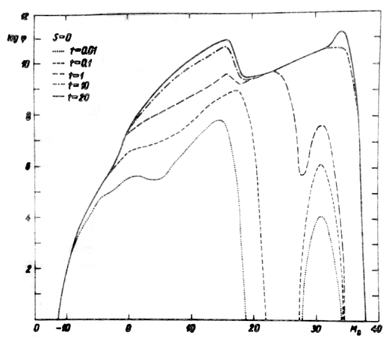
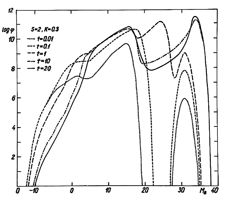
Figure 3: The dependence of the luminosity function of galaxies in B system on the age of the galaxy $t$ in billion years. As argument we use the absolute magnitude in B system. Star formation function parameters are taken as follows: left : $S=0$, $n=2.33$, $M_{0}=0.03\,M_{\odot}$, $R=5\,M_{\odot}$ per year; right $S=2$, $K=0.3\times 10^{9}$ years. The mass of the galaxy is $M=10^{11}\,M_{\odot}$.

To get tracks for metal deficit stars we added to tracks for $Z=0.02$ corrections:

$$\Delta\,\log\,t=-0.22,\hskip 5.69054pt\Delta\,\log\,L=0.25.$$ (23)

Correction for $\log\,T_{e}$ was changed from zero-age main sequence point 0.085 until the tip of the giant branch at 0.200. In addition, the blue end of the horizontal giant branch was fixed at point $\log\,T_{e}=4.25$, and in the luminosity by $\Delta\,\log\,L=-0.15$ lower than for stars of normal composition. These corrections were found using tracks by Demarque et al. (1971), and photometric observations by Sandage (1970). We attributed these corrections to stars of composition $Z=0.001$.

2 Model results

The following functions were calculated: luminosity function, integrated luminosity in solar units and magnitudes, the contribution of stars of different luminosity to the summed luminosity, mass-to-light ratio. All functions were found in bolometric units and in photometric system UBVRIJKL. Also the distribution of energy in spectra of model galaxies using calibrations according to Table IV by Johnson (1966a). Table 2 gives a logarithm of the luminosity in ergs for a star of zero magnitude in UBVRIJKL system, and the intrinsic colour of the Sun according to Mendoza (1968).

The amount of calculations and output results was rather large. We show the main results in a graphical form in Figs. 3 to 9. The dependence of some quantities (luminosity, mass-to-light ratio, colour) on time (age of the model galaxy) is not very smooth. The reason for this behaviour is due to the use of a discrete distribution of masses of stars in the program. For plotting we used in Figs. 3 to 8 smoothed functions.

The most interesting model calculation results are colour indexes and energy distributions in spectra, as these quantities can be directly compared with observations. This comparison is done in the next section.

4 Analysis of results

In this section we discuss various functions and parameters of model galaxies with observations.

A. Luminosity function. An important property of luminosity functions is the continuation of the function toward faint stars to very low luminosities. This suggests that there exist stars of very low luminosity, contrary to earlier estimates by van Rhijn and Luyten, who suggested that stars of magnitude fainter than $M=16$ are very rare.

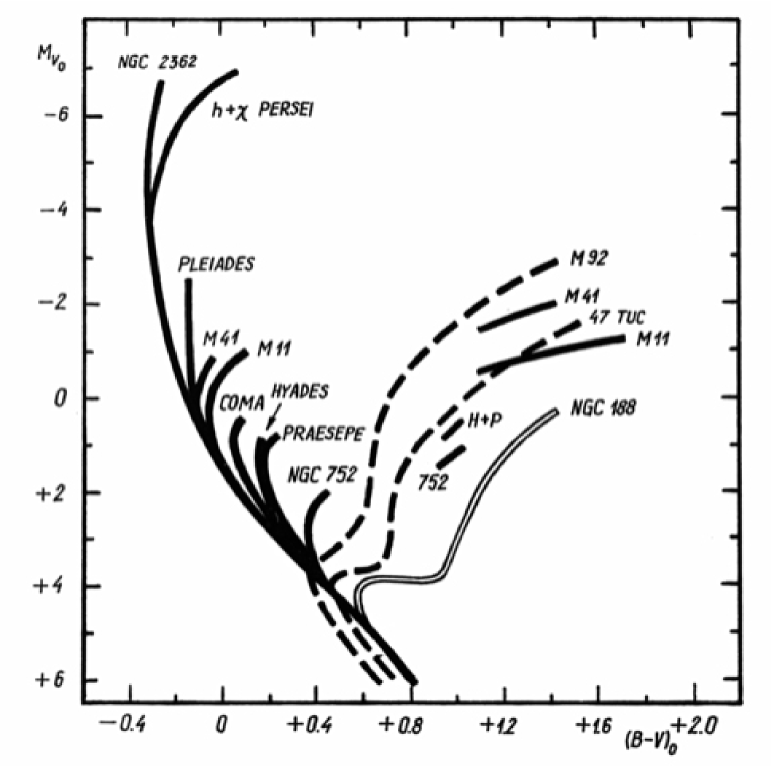
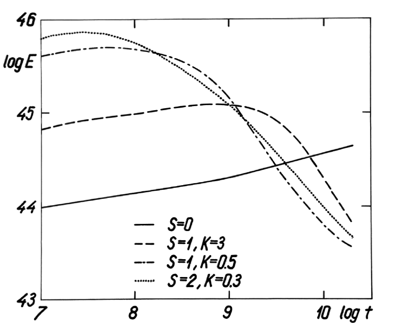
Figure 4: Left: Colour-magnitude diagrams for selected star clusters. Right: Integral bolometric luminosities of galaxies of mass $M=10^{11}\,M_{\odot}$ as function of the age $t$ in years for various parameters $S$ and $K$ of star formation function.

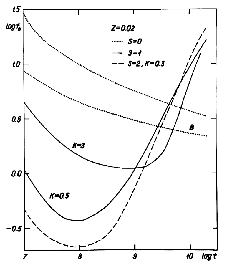
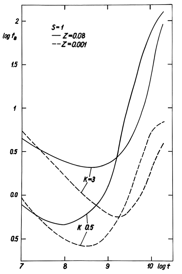
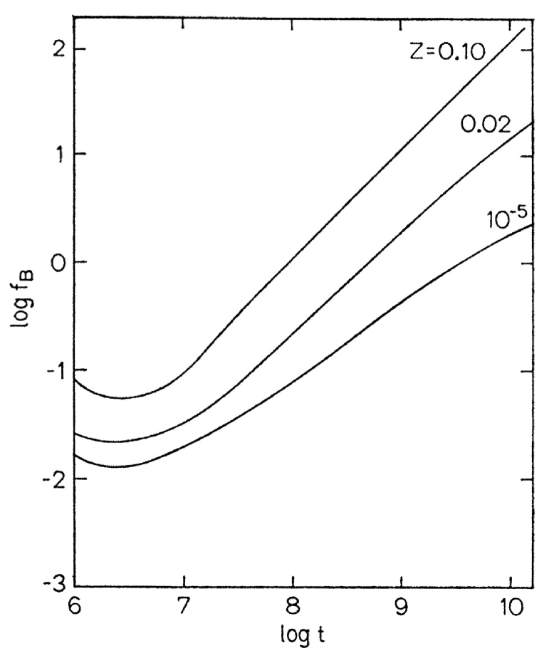
Figure 5: Left: Mass-to-light ratio of galaxies, $f_{B}=M/L_{B}$, as function of the age $t$ for various parameters of the star formation function. In central and right panels data are given for extremal values of the metal content $Z$.

In very young star systems, stars of high luminosity are dominating, there exist also pulsars – supernova remnants. In young systems low mass stars are still in the stage of gravitational contraction, their contribution to the luminosity of the system, is surprisingly high. With increasing age of the system, the luminosity of red dwarfs decreases, the number of pulsars increases, and first white dwarfs appear. All these developments increase the number of stars of low luminosity. During the whole existence of our Galaxy, the luminosity of some types of stars has decreased by 38 magnitudes.

B. Bolometric luminosities. Tinsley (1968) calculated models of the evolution of galaxies in the age interval 1 to 12 billion years with step 1 billion years. Our models cover a much larger age interval that allows to follow the early phase of the evolution of galaxies. In the early stage the luminosity of galaxies increases very rapidly, but this stage is very short. In our models we used a constant density of matter during the evolution. In real galaxies in the early stage of the evolution the density was smaller, and galaxies contracted during the evolution. The contraction of the central region is fast, only a few millions of years. For this reason, the overall change of the luminosity depends only slightly on the variability of the density.

It is interesting to note that the maximal luminosity of the galaxy was approximately a hundred times higher than in the present epoch (for a galaxy with constant mass).

C. Mass-to-light ratios. The dependence of the mass-to-light function on chemical composition and star formation rate parameters is in good agreement with expectations, see Fig. 5. The general diapason of the function $f=M/L$ of old populations of different composition allows to explain differences of this function for globular clusters and elliptical galaxies of various mass. Variations needed to explain these very different populations can be obtained by changing parameters of star formation function and respective evolutionary tracks in reasonable limits.

D. Colours of model galaxies and star clusters. The dependence of $U-B$ and $B-V$ colours of model galaxies on the age is shown in Fig. 6, and in a two-colour diagram in Fig. 7. To compare our results with observations, we compiled similar data for real clusters. Stars of a given cluster have identical chemical composition and age, and can be used to check models of evolution of stars of different mass. Similarly, star clusters can be used to check evolutions of whole stellar systems. For this purpose, instead of individual stars we have to compare integrated parameters of model clusters with integrated parameters with real clusters. We show in Fig. 4 colour-magnitude diagrams for selected star clusters of various ages and chemical composition.

Table 4: Data on clusters

References are: 63 Newell et al. (1969), 101 Sandage (1970), 105 Arp (1964a), 106 Strom & Strom (1970), 107 Sandage (1969), 108 Helfer et al. (1959), 109 Eggen (1970), 110 Gunn & Kraft (1963), 111 Wallerstein & Conti (1964), 112 Philip (1970), 113 Nissen (1970a), 114 Conti & Strom (1968), 115 Nissen (1970b), 116 Alexander (1967), 117 Demarque & Schlesinger (1969), 118 Aizenman et al. (1969), 119 Eggen (1968), 120 Demarque & Miller (1969), 121 Spinrad et al. (1970), 122 Eggen (1969b), 123 Spinrad & Taylor (1971).

We compiled a list of star clusters with known integrated intrinsic colours, $I(U-B)_{0}$ and $I(B-V)_{0}$. Our compilation is given in Table 4. The age of clusters was found using the turn-off point of main sequence, as seen in Fig. 1. For a number of clusters, it was possible to find estimates of the metal content. We give in the Table mean metal content as follows:

$$[Fe/H]=(\log\,Fe/H)_{star}-(\log\,Fe/H)_{\odot}.$$ (24)

As usual, we accept the position that the iron content characterises the content of all heavy elements. The metallicity parameter $Z$ is related with the $He/H$ parameter as follows:

$$\log\,Z/Z_{\odot}=[Fe/H],$$ (25)

where we take $Z_{\odot}=0.02$ according to Sandage & Eggen (1969).

Table 5: Mean metallicity and colour indexes

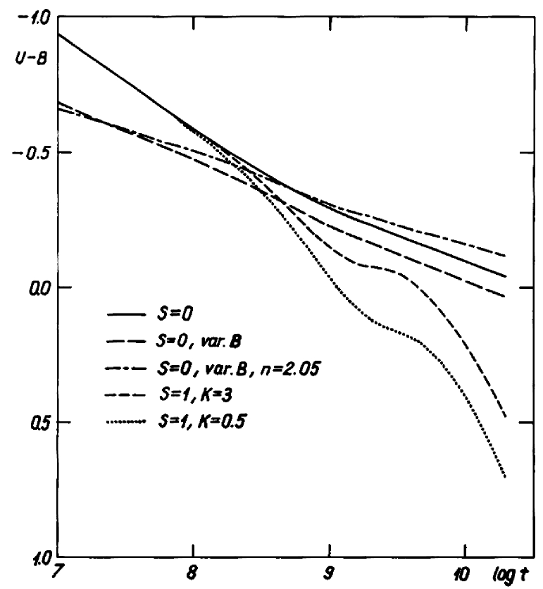
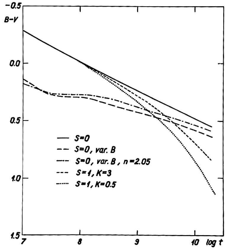
Figure 6: The dependence of colour $U-B$ (left) and $B-V$ (right) of model galaxies on the age for various star formation rate parameters.

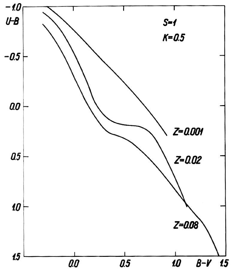
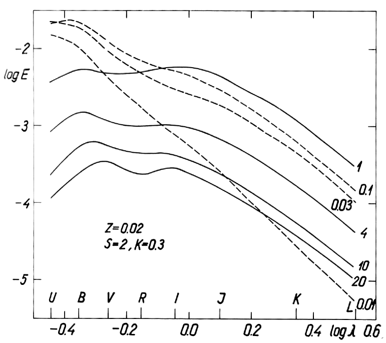
Figure 7: Left: Evolution tracks of model galaxies of different chemical composition in a two-colour diagram. Right: The energy distribution in spectra of a model galaxy of mass $10^{11}\,M_{\odot}$ at different age, given in billion years. Wavelength is shown in microns and in watts per cm^-2 $\mu^{-1}$.

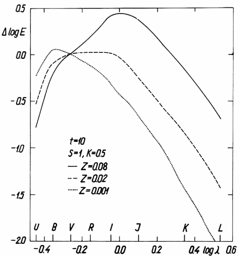
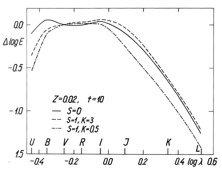
Figure 8: Energy distributions in model galaxies of identical age, $t=10\times 10^{9}$ years, but for different composition (left), and for different parameters of star formation function (right).

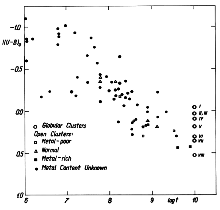
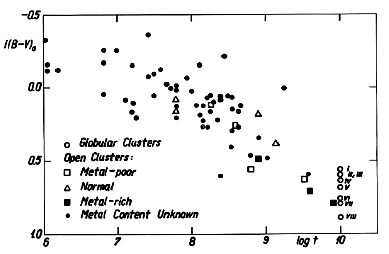
Figure 9: Age dependence of integral colours of star clusters of various ages: $I(U-B)_{0}$ (left) and $I(B-V)_{o}$ (right). Globular clusters are divided into groups according to Morgan metallicity index.

The metal content in globular star clusters changes in rather large limits. There are too few quantitative data on $[Fe/H]$ to find a reliable relation between $[Fe/H]$ and the parameter

$$Q=(U-B)-0.72\,(B-V),$$ (26)

which is often used as the metallicity index (van den Bergh 1967). There are more quantitative data on the Morgan (1959) metallicity type and the $Q$ parameter. Using available data we found mean relations between Morgan type, metallicity index $Q$, and integrated colours of clusters, the results are given in Table 5. Here we give integrated colours, corrected for interstellar reddening, $I(U-B)_{0}$ and $I(B-V)_{0}$, calculated using Eq. (26).

Integrated colours are shown in Fig. 9. As we see, theoretical relations between the colours are in good agreement with observed ones.

E. Energy distribution in spectra of model galaxies of age $t=10\times 10^{9}$ years is shown in Fig. 8 for different compositions and parameters of the star formation function. The distribution is rather similar with the distribution found by Tinsley (1968). Model distributions can be compared with the energy distribution at central regions of elliptical galaxies by Sandage et al. (1969) and Johnson (1966b).

5 Conclusions

We can summarise our results as follows. By choosing in reasonable limits parameters of star formation function, it is possible to calculate model galaxies with integrated characteristics, similar to integrated characteristics of star clusters. Integral parameters, including colours and spectral energy distributions, depend on the age, chemical compositions, and rate of star formation. Model galaxies of identical colour can have ages which differ by an order of magnitude, see Figs. 5 and 8. Our results support the result by Sandage (1963) that blue colour of galaxies is not always an argument to the small age of the system. Our data show that the view by Tinsley (1968) that all galaxies have identical ages can be distorted by the non-optimal choice of parameters of the star formation function.

August 1971

Chapter 24 Star formation function and galactic populations

1 Introduction

In earlier Chapters we discussed the reconstruction of the dynamical and physical evolution of the Galaxy. The rate of star formation was discussed in a general form. Calculations were done for a wide range of parameters of the star formation function.

In the present Chapter we shall discuss the star formation function in more detail. We shall find numerical values of parameters of the function and estimate the dependence of this function on the chemical composition of the interstellar gas. Also, we discuss on the basis of star formation function how stellar populations of various age and composition of the Galaxy could be formed.

An essential parameter of the Galaxy is its age. We start our discussion with an overview of determinations of the age of the Galaxy.

2 The age of the Galaxy

We count the age of galaxies since the moment when star formation in its protogalaxy started. According to the present understanding on the evolution of the Universe, most galaxies formed simultaneously when fluctuations in the expanding primeval cooling matter density were strong enough to start star formation in the densest regions, which became nuclei of forming galaxies.

There exist today at least three independent methods to derive ages of galaxies. The first is based on cosmological considerations: it is clear that ages of galaxies are smaller than the age of the Universe. The age of the Universe can be expressed as follows:

$$T_{U}=\alpha(q_{0})\,H^{-1},$$ (1)

where $H$ is the Hubble parameter (in the present epoch), and $\alpha(q_{0})$ is a dimensionless coefficient, its value depends on the cosmic acceleration parameter $q_{0}$ (and of cosmological density parameters). In Tabel LABEL:Tab23.1 we give some recent determinations of the Hubble constant, and respective ages of the Universe for three values of the acceleration parameter $q_{0}$. If we accept for the cosmological constant a value $\Lambda=0$, and for the acceleration parameter values $q_{0}=0.5$ and $q_{o}=1.5$ (Sandage 1961; Peach 1970), we get the age of the Universe $T_{U}$ values given in Table LABEL:Tab23.1. For comparison we give also the age, corresponding to the acceleration parameter $q_{0}=0$.

Table 1:

$H$ (km s-1 Mpc-1)		$T_{U}$ ($10^{9}$ years)		References
	$q_{0}=0$	$q_{0}=0.5$	$q_{0}=1.5$
95	10.5	6.9	5.3	van den Bergh (1970)
75	13.0	8.7	6.7	Sandage (1968)
47	20.8	13.9	10.7	Abell & Eastmond (1968)

We see that the accuracy of present determinations of parameters $H$ and $q_{0}$ is not sufficient to find the age of the Universe. The uncertainty is even larger when we take into account the possible error in our assumption $\Lambda=0$. Most often it is assumed that the Hubble constant is $H=75$ km s^-1 Mpc^-1, and the acceleration parameter $q_{0}=0.5$, which yields $T_{U}=8.7\pm 1.5\times\,10^{9}$ years.

Another method to estimate the age of our Galaxy is to use determinations of ages of its oldest halo populations. This method can be used for globular star clusters.

Earlier evolutionary tracks in Herzsprung-Russel diagram for globular clusters were calculated using the assumption that the helium content is very low, which yields to ages of the order $15-20\times 10^{9}$ years (Schwarzschild 1958), exceeding the age of the Universe $T_{U}$. Recent data suggest that the helium content in globular clusters is the same as in stars of population I (Rood & Iben 1968; Sandage et al. 1969). This shows that the helium is of primordial origin. New evolutionary tracks are in good harmony with estimates of the age of the Universe from other sources. Table LABEL:Tab23.2 gives a summary of recent determinations of ages of globular clusters. Different determinations vary in reasonable limits. According to Sandage (1970) the probable age of globular clusters is $T=10\pm 0.8\times 10^{9}$ years.

Table 2:

$T$ ($10^{9}$ years)	References
8.5	Rood & Iben (1968)
$11-13$	Iben & Rood (1970b)
9.6	Sandage (1970)
11.6	Sandage (1970)

The most accurate age estimates of the Galaxy come with the radiative isotope method. The idea to use this method to determine the age of the Solar system was expressed by Burbidge et al. (1957). Initially only the isotope $U^{235}$ was used, which gave for the age of the Galaxy $T=6.6\times\,10^{9}$ years, if the uranium was formed rapidly in the early phase of the history of the Galaxy. If the uranium was formed with constant speed, then the isotope age of the Galaxy is $T=11.5-18\times\,10^{9}$ years.

A review of determinations of the age of the Galaxy with the isotope method was given by Dicke (1969). We do not use older determinations of the isotope age of the Galaxy, since the number of isotopes used was too small, and errors in determinations of ages of meteorites were large.

The number of isotopes used in age determinations is increasing and the accuracy in atomic parameters is improving, thus results are now more accurate. The theory of the method is given by Schramm & Wasserburg (1970). The age estimates depend on the speed of the formation of radioactive elements. If we suppose that most radioactive elements were formed rapidly, then the age of the Galaxy is $9\times 10^{9}$ years. If isotopes were formed with constant speed, then the age of the Galaxy increases by a factor of 1.5. This second possibility, however, is excluded by other data (Unsold 1969). For this reason we accept the first alternative. Most recent data on isotope ages are summarised in Table LABEL:Tab23.3.

Table 3:

$T$ ($10^{9}$ years)	References
$8.7\pm 0.7$	Hohenberg (1969)
$9.7\pm 1.0$	Wasserburg et al. (1969)

The mean value obtained with the isotope method is, $T=9.0\pm 0.5\times\,10^{9}$ years. This age can be attributed to the disc of the Galaxy, which according to our estimates is at the speed of the contraction of the Galaxy by $0.5\times\,10^{9}$ years younger than the Galaxy. Thus we get for the whole Galaxy $T=9.5\pm 0.7\,\times 10^{9}$ years.

When we use results of all three methods, we get for the age of the Galaxy $T=9.5\pm 0.75\,\times 10^{9}$ years. Instead, we shall use in further calculations a round value $T=10\times 10^{9}$ years. If $q_{0}=0.5$ and $\Lambda=0$, then this age corresponds to the Hubble constant $H=65$ km s^-1 Mpc^-1.

3 Rate of star formation

The local rate of star formation can be expressed as follows (Schmidt 1959, 1963):

$$R_{l}={{\rm d}\rho_{s}\,\over{\rm d}t\,}=\gamma\rho_{g}^{2},$$ (2)

where $\rho_{s}$ and $\rho_{g}$ are densities of stars and gas, respectively, $\gamma$ is a coefficient with dimension (density x time)^-1, and we accepted the star formation parameter, $S=2$. Since ${\rm d}\rho_{g}\,=-{\rm d}\rho_{s}\,$, then we can write Eq. (2) as follows:

$$-{{\rm d}\rho_{g}\,\over\rho_{g}^{2}}=\gamma\,{\rm d}t\,.$$ (3)

Let us assume that the full density of matter in the given element of space is constant and that at the initial time $t=0$ the whole matter was in a gaseous form. After integration we get:

$$\rho_{g}={\rho\over 1+\tau},$$ (4)

where

$$\tau=t/K$$ (5)

is the dimensionless time, and the characteristic time is

$$K={1\over\gamma\,\rho}.$$ (6)

Using (4) we can write the equation (2) as follows:

$${{\rm d}\rho_{s}\,\over{\rm d}t\,}=\gamma\,{\rho^{2}\over(1+\gamma\,\rho\,t)^{2}}={\rho\over K}\,{1\over(1+\tau)^{2}}.$$ (7)

Integrating Eq. (2) along the line of sight we get in a similar way

$$P_{g}={P\over 1+\tau}$$ (8)

and

$${{\rm d}P_{s}\,\over{\rm d}t\,}=\kappa\,{P^{2}\over(1+\kappa\,P\,t)^{2}}={P\over K}{1\over(1+\tau)^{2}},$$ (9)

where $P_{g}$ and $P_{s}$ are projected densities of gas and stars, $P=P_{g}+P_{s}$,

$$\kappa={\gamma\over 2\,\zeta^{*}},$$ (10)

and

$$K={1\over\gamma\bar{\rho}}.$$ (11)

In the last equation

$$\bar{\rho}={P\over 2\zeta^{*}}$$ (12)

and

$$\zeta^{*}={P_{g}\over 2\bar{\rho_{g}}},$$ (13)

where

$$\bar{\rho_{g}}={\int\,\rho_{g}\,{\rm d}P_{g}\,\over P_{g}},$$ (14)

and integration is over the line of sight. If $\rho_{g}$ has normal distribution, then

$$\zeta^{*}=\sqrt{\pi}\,\zeta,$$ (15)

where $\zeta$ is the dispersion of positions of gas particles along the line of sight.

We use now the modified exponential density profile

$$\rho(a)=h\exp\left[x_{0}-\left[x_{0}^{2N}+\left({a\over k\,a_{0}}\right)^{2}\right]^{1/(2N)}\right],$$ (16)

where $h$ and $k$ are normalising constants, $x_{0}$ and $N$ are structural parameters, and $a_{0}$ is the major semiaxis of the equidensity ellipsoid. The parameter $x_{0}$ regulates the density law near the centre of the ellipsoid. If we take $x_{0}=0$, we get the usual exponential density profile

$$\rho(a)=h\exp\left[-\left({a\over k\,a_{0}}\right)^{1/N}\right].$$ (17)

If the line of sight is directed along the rotation axis, we get for large distance $R$

$$\zeta=\epsilon\sqrt{N}R\left({k\,a_{0}\over R}\right)^{1/(2N)},$$ (18)

and for the centre, $R=0$

$$\zeta=\epsilon\sqrt{N}\,k\,a_{0}x_{0}^{N-1\over 2}.$$ (19)

Integrating over the whole volume of the system we get

$$\mathfrak{M}\,_{g}={\mathfrak{M}\,\over 1+\tau},$$ (20)

and for the rate of star formation

$$R={{\rm d}\mathfrak{M}\,_{s}\,\over{\rm d}t\,}=\lambda{\mathfrak{M}\,^{2}\over(1+\lambda\,\mathfrak{M}\,\,t)^{2}}={\mathfrak{M}\,\over K}{1\over(1+\tau)^{2}},$$ (21)

where $\mathfrak{M}\,_{g}$ and $\mathfrak{M}\,_{s}$ are full masses of gas and star in the galaxy, and

$$\lambda=\gamma/V^{*},$$ (22)

and $K$ is expressed by Eq. 11. For the mean density we get now

$$\bar{\rho}={\mathfrak{M}\,\over V^{*}},$$ (23)

where

$$V^{*}={\mathfrak{M}\,_{g}\over\bar{\rho}_{g}},$$ (24)

and

$$\bar{\rho}_{g}={\int\,\rho_{g}\,{\rm d}\mathfrak{M}\,_{g}\,\over\mathfrak{M}\,_{g}}.$$ (25)

Now we introduce standardised density and mass functions and get for the mean density

$$\bar{\rho}={1\over 4\pi\,\epsilon}{\mathfrak{M}\,\over a_{0}^{3}}\,\chi,$$ (26)

where

$$\chi=\int_{0}^{\infty}\left({\mu_{0}\over\alpha}\right)^{2}\,{\rm d}\alpha\,,$$ (27)

and $\epsilon$, $a_{0}$, and the standardised mass function $\mu_{0}$ describe the gas population, and only $\mathfrak{M}\,$ is the whole mass of the galaxy. Here we used the designation $\alpha=a/a_{0}$, where $a$ is the major semiaxis of the density ellipsoid, and $\mu(a)\,{\rm d}a\,=4\pi\,\epsilon\,a^{2}\,\rho(a)\,{\rm d}a\,$ is the mass function – the mass of an ellipsoidal sheet of thickness ${\rm d}a\,$ and ratio of vertical to horizontal axes $\epsilon$. If the gas is distributed according to the exponential law, then we get

$$\chi={N\,h^{2}\,k^{3}\over 2^{3N}}\,\Gamma(3N).$$ (28)

For a series of $N$ values the function $\chi$ is given in Table LABEL:Tab23.4.

Table 4:

$N$	$\chi$
0.5	0.5555
1	0.5000
2	0.7146
3	0.6124
4	0.7596
5	0.9708
6	1.2644

4 Determination of the parameter $\gamma$

Direct observations allow to determine the full mass of the galaxy, $\mathfrak{M}\,$, the mass of the gas, $\mathfrak{M}\,_{g}$, and the mean density, $\bar{\rho}$. In external galaxies, it is possible to find also the projected density of gas and young stars. In our Galaxy it is possible to find the spatial density of gas and young stars. In all equations, connecting these quantities, the parameter $\gamma$, characterising the rate of star formation, plays an important role. To determine the value of the parameter $\gamma$ there are several integral and differential methods. We shall apply the integral method using data on M31 and the Small Magellan Cloud (SMC), and the differential method using data on SMC.

Let us use first the integral method. Basic data used in calculations are given in Table LABEL:Tab23.5.

Table 5:

Quantity	Units	M31	SMC
$\mathfrak{M}\,_{H}$	$10^{9}\,M_{\odot}$	3.7	0.48
$\mathfrak{M}\,_{g}$	$10^{9}\,M_{\odot}$	5.3	0.68
$\mathfrak{M}\,$	$10^{9}\,M_{\odot}$	110	2.4
$K$	$10^{9}$ years	0.50	4
$a_{0}$	kpc	9	1.5
$\epsilon$		0.016	0.5
$\bar{\rho}$	$M_{\odot}$/pc3	0.38	0.062
$\gamma$	$\left({M_{\odot}\over pc^{3}}\times 10^{9}\,yr\right)^{-1}$	5.3	4.0

The mass of hydrogen of M31 was taken from our recent model of M31 Einasto (1969b). The mass of hydrogen in SMC was taken from Hindman (1967). In the calculation of the full mass of gas, the hydrogen parameter of chemical composition was taken $X=0.70$. The total mass of M31 was taken equal to the sum of its disc and flat populations. The distribution of densities of these populations is similar to the distribution of gas. The mass of SMC and its effective radius $a_{0.5}$ (in de Vaucouleurs spirit) are taken from de Vaucouleurs (1962). From $a_{0.5}$ we found the harmonic radius $a_{0}$, accepting in the generalised exponential model the shape parameter $N=0.5$.

The axial ratio of the density ellipsoid of the M31 gas was taken as equal to $\epsilon=0.016$ in analogy to our Galaxy (Einasto 1970a, 1972a). It was calculated using Eq. (18), which for $N=0.5$ yields

$$\epsilon={\sqrt{2}\,\zeta\over k\,a_{0}}.$$ (29)

We calculated the dispersion of $z-$coordinates, $\zeta$, using densities of hydrogen by Schmidt (1957a), with result $\zeta=100$ pc. Effective radius of the gas population was taken equal to $a_{0}=8$ kpc, parameter $k$ according to tables by Einasto & Einasto (1972b, a). These calculations gave the value $\epsilon=0.0157$.

Table LABEL:Tab23.5 shows that values of the parameter $\gamma$ for M31 and SMC are rather similar in spite of the very different type of these galaxies.

Now we shall find the parameter $\gamma$ applying a differential method, using data on young stars and projected density of gas in SMC.

From Eq. (8) to (10) we get

$${{\rm d}P_{s}\,\over{\rm d}t\,}={\gamma\over 2\,\zeta^{*}}P_{g}^{2}.$$ (30)

We found the projected density of the gas $P_{g}$ from the hydrogen density $P_{H}$ (Hindman 1967), accepting the chemical abundance parameter $X=0.70$. Parameter $\zeta^{*}$ characterises the distribution of gas clouds along the line of sight, and was found as follows. Fig. 2 by Hindman (1967) shows that hydrogen is concentrated to clouds having approximately a round form. This hints to the spherical form of the hydrogen population (SMC as a total has a flattened form). The hydrogen population has approximately normal distribution (its shape parameter of the modified exponential function is $N=0.5$). This allows to find effective radii $a_{0}$ of gas clouds, and from these data the dispersion of $\zeta$ and parameter $\zeta^{*}$. Values found for individual clouds vary between $2\,\zeta^{*}=1.0$ kpc to 2.0 kpc; for the mean we accepted $2\,\zeta^{*}=1.6$ kpc. Following Hindman (1967) we accepted the distance to SMC $d=60$ kpc.

Next we have to find the projected density of stars formed in unit time, $R_{P}={\rm d}P_{s}\,/{\rm d}t\,$.

Sanduleak (1968) found from spectral observations the distribution of bright stars of various spectral types in SMC. His list can be considered as complete up to magnitude $m_{pg}=13.0$, corresponding to $B=13.1$ (Schmidt-Kaler 1965). For distance modulus $(m-M)_{ph}=19.0$ (van den Bergh 1965) this corresponds to completeness of data up to $M_{B}=-6.0$.

According to Sanduleak (1968), the total number of stars brighter than $M_{B}=-6.0$ is $P=126$. We can compare this number with the expected number from the theoretical star formation model. We take in the model $S=0$, which corresponds to constant star formation rate $R^{\circ}=5$ solar masses in a year. Using the luminosity function $\varphi(M_{B})$ we found that the expected number of stars brighter than $M_{B}=-6.0$ is $P^{\circ}=25\,500$. The actual star formation rate in SMC is $P^{\circ}/P=200$ times lower than in our model. This leads to SMC star formation rate $R=0.025\,M_{\odot}$ in year.

This star formation rate of SMC can be underestimated, since the Sanduleak (1968) list did not include supergiant stars. To estimate the possible selection effect, we calculated the star formation rate $R$, applying Eq. (21), and used as characteristic time of star formation parameter $K$ our result from Table LABEL:Tab23.5. We found $R=0.050\,M_{\odot}$ a year. If this estimate is correct, then the star formation rate, found from Sanduleak (1968) list of stars, is to be multiplied by a factor of two.

Sanduleak (1969) found the distribution of stars brighter than $m_{ph}=13$ for unit surface density, $P_{l}$. It is clear that

$${Q\,P_{l}\over P^{\circ}}={R_{P}\over R^{\circ}},$$ (31)

where $Q\approx 2$ is the correction factor described above. We used this equation together with Eq. (30) to estimate the parameter $\gamma$. Sanduleak (1969) got for the power index of the star formation rate $S=1.84\pm 0.14$, which is almost equal to the value we accepted, $S=2$. Using Sanduleak (1969) distributions of $P_{l}$ and $P_{g}$, and calibrating gas densities to surface densities, we got $\gamma=2.9$ in units $(M_{\odot}\,pc^{-3}\,Gyr)^{-1}$.

This estimate of the parameter $\gamma$ is in good agreement with data given in Table LABEL:Tab23.5. We accept a mean value of all data,

$$\gamma=4\,(\mathfrak{M}\,_{\odot}\,pc^{-3}\,Gyr)^{-1}.$$ (32)

Our result depends on the age of SMC (we accepted $t=10^{10}$ years), and on the mean axial ratio of the equidensity ellipsoid $\epsilon$ of M31 gas. If we take for the age of SMC two times lower value, and for $\epsilon$ of M31 gas two times larger value, then the parameter $\gamma$ increases by a factor of two. However, in this case the selection factor $Q$ also increases by a factor of two, which is not acceptable. But we can check this result in another way. The total luminosity of young stars in M31 is in good agreement with our model using parameters $S=2$ and $K=0.25$, and using the total mass of M31. If we use only the mass of the disc of M31, then a good agreement is obtained using $K=0.5$. The luminosity of young star population depends on the star formation rate, which depends on the present mean density $\bar{\rho}$. Using data on gas density in M31, we found for the parameter $\gamma$ a value, close to the value in Eq. (32). In summary, we conclude that there are no reasons to accept for SMC an age smaller than for other galaxies, and for the mean axial ratio of the gas population a value, different from the present one.

Finally, we note that recently Hartwick (1971) found for the star formation parameter for M31 a value $S=3.5\pm 0.12$, using a method similar to the Sanduleak (1969) method. He used Roberts (1966) data on the distribution of neutral hydrogen, and Baade & Arp (1964) data on the distribution of ionised hydrogen as an indicator for the presence of young stars. The theoretical basis of his analysis was criticised by Talbot (1971). However, more important is the effect of antenna smoothing, not used by Roberts (1966) in the determination of the hydrogen distribution. In this way, the hydrogen distribution was strongly smoothed without any peaks of densities along spiral arms, see Einasto (1972b). If the smoothing is properly taken into account, the value of the parameter $S$ becomes fully normal.

5 The dependence of the star formation rate on chemical composition of the gas

The basis of our present understanding of the synthesis of chemical elements in the Universe and chemical evolution of galaxies was presented by Burbidge et al. (1957). Authors demonstrated that all chemical elements heavier than hydrogen are synthesised inside stars as a result of various nuclear processes. Part of synthesis products are expelled from stars, where in this way the interstellar gas is enriched by heavier chemical elements. A bit later it was understood that similarly to hydrogen, helium also has a primordial origin, and only elements heavier than helium are produced in stars. Various nuclear processes and problems of the chemical evolution of galaxies are subjects of intensive studies.

The synthesis of elements heavier than helium takes place in all stars with nuclear activity. The most important factor in the enrichment of interstellar medium with heavy elements are massive stars, which after their active life explode as supernovae. During the explosion, elements of high atomic weight are produced. The study of stars of various chemical compositions and ages gives us information on the synthesis of heavy elements and the star formation function at various stages of the evolution of galaxies.

The possibility of the use of compositions of stars of various age to study the star formation history was explored by van den Bergh (1961). He noted that already in the early phase of the evolution of the Galaxy, the chemical abundance of some open star clusters was close to the normal composition in the present epoch. This hints to a high activity of supernova explosions in the early phase of Galaxy evolution. The same conclusion was made by Schmidt (1963). The chemical composition of stars and gas in the early phase of the Galaxy evolution was studied by Dixon (1965, 1966). Truran & Cameron (1970) and Cameron & Truran (1971) developed a model of the chemical evolution of the Galaxy. According to their model, in the early phase of the evolution, a large fraction of almost pure hydrogen-helium stars evolved rapidly and enriched the halo gas with heavy elements.

Until recently, the attention of astronomers was directed to understand the chemical aspects of the problem. Relatively little attention was given to possible changes of parameters of the star formation function, which could cause the effects mentioned above.

Based on the arguments, given by Dixon (1965, 1966) and Cameron & Truran (1971), we can conclude that the heavy element content after the initial rapid contraction of the protogalaxy was relatively high, about three times less than the solar content. To find possible errors of this estimate, let us consider two variants: A) heavy element content at the end of the contraction was $Z_{h}=0.010$, i.e. two times less than the present content, and B) $Z_{h}=0.005$. The mass of the halo of M31 is 10 % of the mass of the whole galaxy (Einasto 1970b, 1972b), let us assume that the relative halo mass of our Galaxy is the same (direct data are less accurate). All heavy elements of the gas in the Galaxy in this epoch (90 % of the total mass of Galaxy) were produced by first-generation stars (10 % of the mass of the Galaxy). If we assume that heavy elements were not consumed by compact objects of the halo, then in variant A the fraction $\psi_{h}=0.090$ of initial stellar mass was expelled from stars as heavy elements. In variant B the fraction is $\psi_{h}=0.045$.

The mean heavy element content in the disc of the Galaxy is $Z=0.02$ (in the present epoch the mean heavy element content of young stars is slightly higher). The mass of the disc is about 53 % of the whole mass of the Galaxy (Einasto 1970a; Einasto & Einasto 1972a; Einasto 1972a). Based on these data, we can calculate the total mass of heavy elements in the disc. When we remove from this amount the mass of heavy elements at the beginning of disc formation, we can find the amount produced by disc stars. We find that in variant A, the fraction of mass of disc stars, expelled as heavy elements, was $\psi_{d}=0.009$, and in variant B $\psi_{d}=0.014$. We conclude that in comparison with halo stars, the effectiveness of the synthesis of heavy elements has decreased in variant A 10 times, and in variant B 3 times.

Can this decrease of the star formation rate be explained by changes of parameters of the star formation function?

Applying the star formation function $F(M)$ of Chapter 22, we can calculate the fraction of stars of large mass. Let us use for disc stars of Galaxy the lower mass limit of forming stars, $M_{0}=0.03\,M_{\odot}$, upper mass limit $M_{u}=100\,M_{\odot}$, the exponent of the mass function, $n=2.333$, and the minimal mass of stars as future supernovae, $M_{SN}=2.6\,M_{\odot}$. The total mass of stars with masses $M\geq M_{SN}$, is for these parameters $E_{d}=0.17$ of the mass of all stars – the disc supernova producing capability. All heavy elements are synthesised by these stars of masses $M\geq M_{SN}$. Accepting for disc stars the heavy element synthesis fraction $\psi_{h}$ as found above, we find that in variant A 5 % of star mass is expelled as heavy elements, and in variant B 8 % of star mass.

Let us now consider possibilities to increase the fraction of heavy elements. There are two possibilities for this: to increase the fraction of massive stars, and to increase the heavy element synthesis capacity of supernova explosions.

The fraction of stars with masses above $M_{SN}$ can be increased by the increase of minimal star forming mass $M_{0}$, and by decreases of index $n$ and supernova mass limit $M_{SN}$. Let us take $M_{0}=0.3\,M_{\odot}$ (this is the maximal possible value from globular cluster data), $n=2$ and $M_{SN}=2\,M_{\odot}$ (only stars of this mass have time to evolve during the time of the contraction of the halo – 1 billion years – to reach the supernova explosion stage). Accepting these parameters we find for the halo supernova producing capability $E_{H}=0.68$, which is four times higher than the disc capability. This is more than needed to explain the heavy element content, needed at the end of halo contraction phase for the variant B, but not large enough for the variant A. A further increase of $M_{0}$ or decrease of $M_{SN}$ are not possible. For this reason, if the variant A of the fraction of mass expelled as heavy elements is to be favoured, then the only possibility to explain the disc heavy element content in the framework of the contracting halo scenario is to decrease $n$ or to increase the effectiveness of the creation of heavy elements during supernova explosions.

Requirements for changes of star formation function parameters are not too restrictive. For this reason, we think that there are no need to accept the hypothesis for the initial prompt formation of all heavy elements, as suggested by Truran & Cameron (1970) and Cameron & Truran (1971).

6 Formation of galaxies and their populations

The Schmidt Eq. (2) allows to explain in a quantitative way the formation of galaxies of various morphological type as well as the formation of galactic populations.

Let us discuss first the formation of galaxies of different morphological type: ellipticals, spirals and irregulars. Galaxies of these types differ from each other by their mean density. Bulges of elliptical and spiral galaxies have high mean density, for the bulge of M31 we found $\bar{\rho}=6\,M_{\odot}\,pc^{-3}$. The mean density of the disc of spiral galaxies is lower by an order, and the mean density of irregular galaxies is lower by another order. Using these mean densities and Eq. (6) we calculated the respective characteristic time $K$, and then using Eq. (20) the change of the relative amount of gas, and from Eq. (21) the rate of star formation $R$. Results of our calculations are given in Figs. 1 and 2.

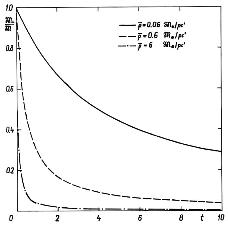
Figure 1: The fraction of gas mass in model galaxies of various mean density.

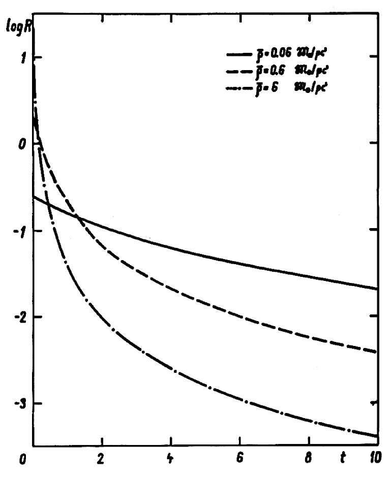
Figure 2: The rate of star formation $R(t)$ in galaxies of different mean densities.

In Fig. 3 we show the change of the total luminosity of the galaxy with time. It was calculated as follows:

$$\mathcal{L}_{B}(t)=\delta\,\int_{t_{0}}^{t}\,R\,{\rm d}t^{\prime}\,,\hskip 28.45274ptt_{0}=\left\{\begin{array}[]{rc}0,&t\leq\Delta\\ t-\Delta,&t\geq\Delta.\end{array}\right.$$ (33)

Here the factor $\delta$ and time interval $\Delta$ were estimated from the comparison of results of calculations with results in Chapter 23 for $K=0.3$. Our calculations suggested that $\Delta$ must be taken as a linear function of time

$$\Delta=0.1+0.14\,t,$$ (34)

where both $\Delta$ and $t$ are expressed in units $10^{9}$ years.

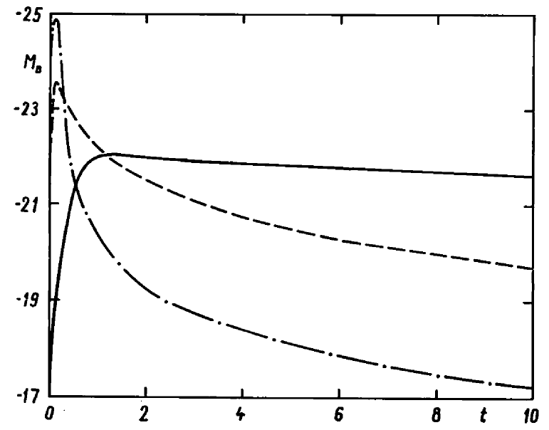
Figure 3: The evolution of galactic total luminosity for galaxies of different mean density. Lines as in Figs. 1 and 2.

Properties of model galaxies for the age $t=10^{10}$ years represent rather well the observed properties of elliptical, spiral and irregular galaxies. This raises the question: How to explain differences in density in these three types of galaxies?

It should be stressed that differences in mean densities can be formed only in the gaseous phase of the evolution of galaxies. Stellar populations are very conservative in this respect, as kinematical and spatial characteristics of the structure of galaxies change very slowly.

One of possible reasons for changes in mean densities could be differences in primeval mass-angular moment distributions. Protogalaxies with low primeval angular moment could contract considerably and form elliptical galaxies. Protogalaxies with high primeval angular moment could not contract in the radial direction. For this reason, these galaxies formed after the contraction phase gas a thin disc, which fragmented due to gravitational instability into spiral arms. Theoretical aspects of the role of mass-angular moment distribution were discussed by Lynden-Bell (1967b), observational aspects were studied by Sandage et al. (1970).

Let us discuss now the formation of galactic populations. First we consider the halo. Using data by Einasto (1970b, 1972b) we found the mean density of halo, $\bar{\rho}=0.13\,M_{\odot}\,pc^{3}$, which yields $K=2\times 10^{9}$ years. At the end of the halo forming the mass of gas was 90 % of the mass of the galaxy, thus $\tau=0.1$. From $\tau$ and $K$ we can find the time of halo formation $t=\tau\,K=0.2\times 10^{9}$ years. This time is in good agreement with our earlier estimate on the halo collapsing time. Different regions of the halo formed at various times, first the central densest region, then more distant and less dense regions, thus the contraction time is a certain mean value.

After the contraction phase, the remaining gas obtains the form which is close to its present form. Thus, we do not make a considerable error when we consider the projected density of gas, $P(A)$, as time independent. Based on these arguments, we consider the mean thickness of gas, $\zeta^{*}$, also as time independent. Using Eq. (9) we find that the projected density of stars, formed in the time interval $\Delta\,t$ at moment $t$ as follows:

$$\Delta\,P_{s}=\gamma{P^{2}\over 2\,\zeta^{*}}{\left[1+\gamma{P\over 2\zeta^{*}}\,t\right]^{-2}}\,\Delta\,t.$$ (35)

Time in the equation is to be counted not from the formation of the whole galaxy but from the beginning of the formation of the bulge and disc.

This equation allows to explain quantitatively the subsequent formation of populations of increasing sizes. If $t$ is small, then $\tau=\gamma P\,t/(2\zeta^{*})\ll 1$, and we have

$$\Delta\,P_{s}=\gamma{P^{2}\over 2\zeta^{*}}\,\Delta\,t.$$ (36)

Due to very rapid decrease of $P(A)$ with increasing $A$ star formation occurs initially only in central regions –- in this way the nucleus forms. But in central regions of the galaxy, the density of the gas decreases rapidly. For this reason, according to Eq. (35), the central density of the following population also decreases. When $\tau\gg 1$, then we get for the projected density using Eq. (8)

$$P_{g}\approx{2\,\zeta^{*}\over\gamma\,t}.$$ (37)

The density distribution of galactic populations can be described by the modified exponential profile with $\nu=1/N\leq 1$. Based on Eqs. (15) and (18) we see that in this case the parameter $\zeta^{*}$ decreases with increasing distance from the centre. In this way during later phases of galactic evolution, the density of gas in central regions of galaxies gets lower than in more distant regions. This situation is exactly observed in spiral galaxies like M31 (Einasto 1970b, 1972b). The active process of star formation moves from central regions to more distant ones, and the mean radius of recently formed galactic populations increases. In peripheral regions of spiral galaxies, the gas density is very low, and the star formation process has low intensity. Thus, the fraction of gas in the total projected density decreases with distance, see Eq. (8). For M31 at distance 25 kpc from the centre we obtained: $2\,\zeta^{*}=570$ pc, and $P=5\,\mathfrak{M}\,_{\odot}/pc^{2}$, which yields $P_{g}/P=0.75$.

The star formation function gives us the possibility to determine the distribution of galactic populations according to mass.

Let us discuss first the mass distribution of the disc populations of our Galaxy. We integrate Eq. (21) in time from $t=t_{i}-\Delta$ to $t=t_{i}$:

$$\mathfrak{M}\,_{Si}=\int_{t_{i}-\Delta}^{t_{i}}R\,{\rm d}t\,=\mathfrak{M}\,_{S}(t_{i})-\mathfrak{M}\,_{S}(t_{i}-\Delta),$$ (38)

where $\mathfrak{M}\,_{Si}$ is the mass of stellar population $i$, and $\mathfrak{M}\,_{S}(t_{i})=\mathfrak{M}\,-\mathfrak{M}\,_{g}(t_{i})$ is the total mass of stars of the Galaxy at moment $t_{i}$, and the mass of gas $\mathfrak{M}\,_{g}(t_{i})$ is calculated using Eq. (20).

In calculations, we made the following simplifying assumptions. Effective radius of all disc subsystems was taken as equal to $a_{0}=6.45$ kpc in accordance with our model described in Chapter 7. Structural parameters of all subsystems were also taken as equal: $N=1$, $x_{0}=0$. The flattening parameter of the gas was taken equal to $\epsilon=0.0157$, in accordance with the results discussed above. The characteristic time of disc star formation was found using Eq. (11), where the mean density $\bar{\rho}$ was calculated using Eq. (26). We accepted the full mass of the disc $\mathfrak{M}\,=108\times 10^{9}\,\mathfrak{M}\,_{\odot}$, and found $\bar{\rho}=1.0\,\mathfrak{M}\,_{\odot}\,pc^{-3}$ and $K=0.25\times 10^{9}$ years. The total age of the disc of the Galaxy was taken equal to $9\times 10^{9}$ years, and the time spent on the formation of disc subpopulations was taken as equal to $\Delta=10^{9}$ years. Results of calculations are given in Table LABEL:Tab23.6. We see that most subpopulations of disc stars formed during the first billion years after the start of disc formation.

Table 6:

$t_{i}$	$\epsilon_{i}$	$\mathfrak{M}\,_{Si}/\mathfrak{M}\,$	$\mathfrak{M}\,_{Si}/\mathfrak{M}\,$
$10^{9}\,a$		$K=0.25$	$K=0.60$
8.5	0.120	0.8000	0.6250
7.5	0.098	0.0889	0.1442
6.5	0.083	0.0342	0.0641
5.5	0.070	0.0181	0.0362
4.5	0.057	0.0112	0.0233
3.5	0.045	0.0076	0.0162
2.5	0.035	0.0055	0.0120
1.5	0.025	0.0042	0.0092
0.5	0.018	0.0033	0.0073
0.0	0.016	0.0270	0.0625

In Chapter 7 we obtained the relationship between the age of populations and the flattening parameter $\epsilon$ of iso-density surfaces. Using this relationship we calculated mean $\epsilon$ values for disc subpopulations, results are given in Table LABEL:Tab23.6. Using mass, radius, flattening and structural parameters of subpopulations we can calculate the density, and by summing over all subpopulations, find the total matter density. We made these calculations for the region near the Sun. Adding to this value the density of population II (halo), which according to Oort (1958) is $\rho_{II}=0.0015\,M_{\odot}\,pc^{-3}$, we get for the mass density in the Solar vicinity

$$\rho_{\odot}=0.065\,M_{\odot}\,pc^{-3}.$$ (39)

Using Oort constants $A=15$ km/sec/kpc and $B=-10$ km/sec/kpc we find for the Kuzmin parameter a value

$$C=61\leavevmode\nobreak\ km/sec/kpc.$$ (40)

We get the total mass of interstellar matter

$$\mathfrak{M}\,_{g}=2.9\times 10^{9}\,M_{\odot},$$ (41)

and the density of interstellar matter in the Solar vicinity, $\rho_{g}=0.010\,M_{\odot}\,pc^{-3}$.

The comparison of these results with direct density estimates discussed in Chapter 7 shows that all quantities are underestimated except the total mass of gas, which according to Westerhout (1957) is $\mathfrak{M}\,_{g}=1.4\times\,10^{9}\,M_{\odot}$.

To find possible reasons for this disagreement, we repeated calculations using the gas density in Solar vicinity, $\rho_{g}=0.023\,M_{\odot}\,pc^{-3}$. For the parameter $K$ we got a value $K=0.6\times 10^{9}$ years. Results of calculations are given in Table LABEL:Tab23.6. For the total mass density in Solar neighbourhood we got now $\rho_{g}=0.082\,M_{\odot}\,pc^{-3}$, which yields Kuzmin parameter value $C=68$ km/sec/kpc, and total gas mass in the Galaxy, $\mathfrak{M}\,_{g}=6.8\times 10^{9}\,M_{\odot}$.

We see that values of the Kuzmin parameter and total density are fully acceptable, but the total gas mass is too large. We recall that the total gas mass of M31 is only $\mathfrak{M}\,_{g}=5.3\times\,10^{9}\,M_{\odot}$, see Chapter 20. Andromeda galaxy M31 is about 1.5 times more massive than our Galaxy. If relative fractions of gas in both galaxies are equal, then the gas mass of our Galaxy would be $\mathfrak{M}\,_{g}=3.5\times\,10^{9}\,M_{\odot}$. However, there exists arguments suggesting that the relative gas content of our Galaxy is lower than in M31. The linear size of M31 is about 15 % larger than the size of our Galaxy, mutual distances of neighbouring spiral arms of M31 are about two times larger than in our Galaxy (see Chapter 19 and Westerhout (1957)). For this reason, the estimated total mass of gas in Galaxy Eq. (41) is fully acceptable (observational estimate by Westerhout (1957) is probably underestimated, as well as the total mass of Galaxy according to Schmidt (1956)). The first variant of the distribution of masses of disc subpopulations should be closer to reality. How can we explain low values of gas density and total density in Solar neighbourhood found for this variant?

Recently Woolley et al. (1971) demonstrated on the basis of statistics of nearby stars that the relative number of young stars in Solar vicinity is larger than expected on the basis of the hypothesis that the rate of star formation is constant. In other words, the Sun is located in a region of enhanced star forming intensity. The enhanced star forming activity in Solar neighbourhood is supported by the presence of Gould Belt, as well as by the fact that the Sun is located inside a spiral arm of Galaxy (Becker 1970). Apparently, this allows to explain the disagreement between our theoretical density estimate in a smooth Galaxy model, Eq. (39) and observations.

We conclude that the star formation function allows to explain satisfactorily both integral properties of galaxies as well as properties of galactic populations. The general picture of galaxy evolution is similar to the view by Sandage et al. (1970).

October 1971

Chapter A.1 Epilogue

The defence of the Thesis on March 17, 1972 was successful. However, two related problems remained — it was impossible to reproduce the observed rotation curves of galaxies with known stellar populations, and data on mass-to-light ratios of populations were uncertain. For this reason, I started searches to find solutions to these open questions immediately after the defence. The story of events after the defence of the Thesis is described in detail in my book (Einasto 2014) and in the review paper (Einasto 2018). Here I give a short overview of the development of ideas directly connected with the topic of the Thesis.

Both problems are connected with the possibility of the presence of dark matter in galaxies. I had serious reasons to believe that there is only a limited quantity of dark matter in galaxies like our own Galaxy. This problem had been studied by Tartu astronomers long ago. Öpik (1915) was one of the first to study the dynamics of the Galaxy with the goal to find the density of matter in Solar neighbourhood. He understood that due to the flat shape of the Galaxy, the dynamical density can be determined from the comparison of motions and spatial distributions of stars in the vertical direction. He found that the vertical attraction of known stars is sufficient to explain the observed distributions, and that there is no reason to add invisible matter (the term “dark matter” had not yet been suggested). Kuzmin (1955) and his student Eelsalu (1958) repeated this study with new and better data and confirmed Öpik (1915) result. The problem was also discussed by Oort (1960b), who found that the dynamical density near the Sun is larger than found by Kuzmin (1952b, 1955) and Eelsalu (1958). In other words, there is a need for dark invisible matter. Since the matter density and possible presence of dark matter are of fundamental importance, my Tartu collaborator Jõeveer (1968, 1972) made a new analysis, using a completely different method, see Chapter 21. Ages of young stars are known, this allows to find parameters of vertical oscillations of young B stars and cepheids, which led to parameter $C=70$ km/s/kpc and dynamical density $\rho_{dyn}=0.09\,M_{\odot}$/pc³. On the basis of these studies, I supported the classical paradigm with no large amounts of dark matter in the Solar neighbourhood. More accurate recent data support this conclusion (Gilmore et al. 1989).

More data accumulated on rotation velocities of galaxies. New data suggested the presence of almost flat rotation curves of galaxies, thus, it was increasingly difficult to accept my previous solution of the discrepancy with large non-circular motions. I discussed the problem with my colleague Enn Saar in spring 1972, who suggested abandoning my earlier idea that galaxies have relatively sharp boundaries but may have extended envelopes.

The possible presence of dark matter in the Galaxy in Solar vicinity at least in some quantity was suggested by Oort (1932, 1960b), and in clusters of galaxies by Zwicky (1933), Karachentsev (1966), and Rood et al. (1972). A numerical study of the stability of flat galaxies suggest the presence of massive halos of galaxies (Ostriker & Peebles 1973). Rotation velocity measurements of galaxies by Roberts (1966, 1967, 1969a) and Rubin & Ford (1970) suggest that galaxies have indeed large and massive envelopes. My detailed analysis of properties of known stellar populations demonstrated that no known stellar population can be responsible for flat rotation curves of galaxies. As I discussed in Einasto (2018), the tacit assumption in earlier studies was that the stuff, responsible for this effect in clusters, galaxies in general and near the plane of the Galaxy, is the same everywhere.

After the discussion with Enn, I noticed that here lies a controversy. Dynamical data suggest that eventual dark matter in Solar vicinity is strongly concentrated toward the plane of the Galaxy, thus dissipation is needed for its formation. By contrast, if the rotation of galaxies in outer regions is influenced by a new hypothetical population, then this population should form a large, massive, and an almost spherical population. In particular, for its formation, dissipation is not needed. Different size, shape, mass and dissipation properties suggest a different formation history and nature. Following these considerations, I concluded that there must exist two types of dark matter: the “local dark matter” near the Sun close to the plane of the Galaxy, and the “global dark matter”, forming envelopes of galaxies and clusters of galaxies (Einasto 1972a, 1974a).

To have a better reproduction of observed rotation curves, it would be reasonable to look at which properties the population of global dark matter should have using available data on known stellar populations and galaxy rotation data. To avoid confusion with the known halo population, consisting of old metal-poor stars, I called the new population “corona” (Einasto 1972a, 1974a). To check this possibility, I used my programs to calculate dynamical models of galaxies. It was easy to find a new set of models with one addition component — dark corona. As the first approximation, I assumed that the total mass of the M31 corona is equal to the mass of the sum of known stellar populations (Einasto 1972a, 1974a). I made two versions of models of galaxies in the Local Group and giant elliptical galaxy M87, variant A without corona and variant B with corona, see Fig. 1. This calculation showed that the adding of coronas improves model rotation curves, but not enough.

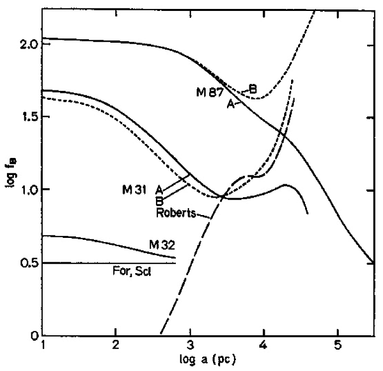
Figure 1: The distribution of mass-to-light ratio, $f_{B}=M/L_{B}$, in galaxies of the Local Group and M87: models without (A) and with (B) dark corona (Einasto 1974a).

I reported new results at the First European Astronomy Meeting in Athens on September 8, 1972 (Einasto 1974a). It was clear that coronas cannot be made of stars because outer stellar populations consist of old halo-type stars with very low mass-to-light ratio, but the mass-to-light ratio of the corona is very high. The coronal matter cannot be in the form of neutral gas, since this gas would be observable. Initially I suspected that it could be ionised hot gas (Einasto 1972a, 1974a). However, the total mass of coronas was not known yet, and the evidence for the presence of coronas was not strong.

So far, I had concentrated my efforts on the study of the structure of galaxies. It was now clear that the environment of galaxies was also important. The dark matter problem was discussed a long time ago in clusters of galaxies. Also masses of groups of galaxies, measured from the velocity dispersion of galaxies, were larger than summed masses of individual galaxies, see Holmberg (1937, 1969) and Karachentsev (1966). A similar discrepancy was found in the Local Group (the M31 - MW system) by Kahn & Woltjer (1959). Reading these papers on the mass discrepancy in clusters, groups and galaxies, I realised that the problem of dark matter in galaxies is the same as in clusters. This allows to find masses and radii of dark coronas of galaxies. I noticed that if galactic coronas are large enough, then companion galaxies should lie inside coronas of the main galaxies. Thus, companion galaxies can be considered as test particles to measure the gravitational attraction of the main galaxy.

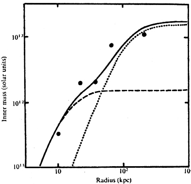
Figure 2: The mean internal mass $M(R)$ as a function of the radius $R$ from the main galaxy in 105 pairs of galaxies (dots). The dashed line shows the contribution of visible populations, the dotted line the contribution of the dark corona, solid line the total distribution (Einasto et al. 1974a).

I collected data for pairs of galaxies. The analysis was soon ready, see Fig. 2. Our analysis suggested that galactic coronas have masses about ten times larger than masses of their visible populations. In those years, Soviet astrophysicists had the tradition to organise Winter Schools. In 1974, the School was held in the Terskol winter resort. I presented my report on the masses of galaxies on January 29, 1974. I stressed in my talk arguments, suggesting that the presence of coronas around galaxies is a general phenomenon. Also, I suggested that galactic coronas probably have the same origin as dark matter in clusters and groups, and that coronas are probably not of stellar origin.

Prominent Soviet astrophysicists like Yakov Zeldovich, Iosif Shklovsky, and others participated in the Winter School. After my talk, the atmosphere was as if a bomb had exploded. For Zeldovich and his group, the presence of a completely new, massive non-stellar population was a surprise. Two questions dominated: What is the physical nature of the dark matter? and What is its role in the evolution of the Universe?

I had to hurry with the publication of our results, since massive halos were already discussed by Ostriker & Peebles (1973) to stabilise orbits of flat population stars. Following a suggestion by Yakov Zeldovich we sent the paper to “Nature” (Einasto et al. 1974a). Soon it was clear that it was just in time. Ostriker et al. (1974) got similar results using similar arguments; their paper was published several months after our “Nature” paper, and has a reference to our preprint. Both papers suggest that the total cosmological density of dark matter in galaxies is about 0.2 of the critical cosmological density.

In the “Nature” paper, we noted that dark matter in clusters cannot be explained by hot X-ray emitting gas, since its mass is insufficient to stabilise clusters. Ostriker et al. (1974) did not notice that dark matter forms a new population of unknown nature; authors write in the discussion that the very great extent of spiral galaxies can perhaps be understood as due to a giant halo of faint stars.

Soon the reaction to the results of both papers appeared: Burbidge (1975) formulated difficulties of the dark corona/halo concept. The main problem is in the statistical character of dynamical determinations of masses of multiple galaxies. If companion galaxies used in mass determination are not real physical companions but random interlopers, as suggested by Burbidge, then the mean velocity dispersion reflects random velocities of field galaxies, and no conclusions on the mass distribution around giant galaxies can be made.

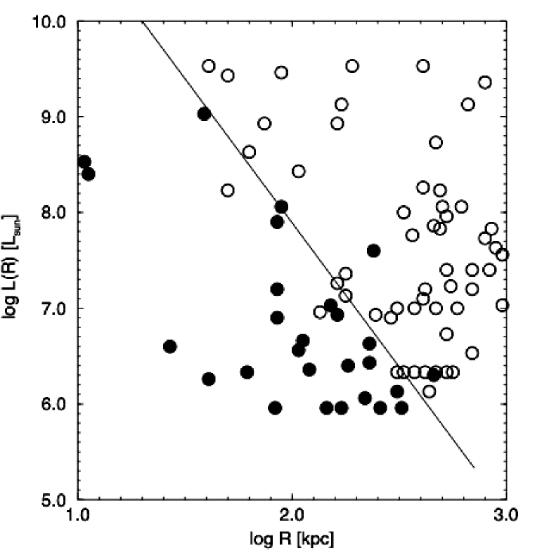
Figure 3: Distribution of luminosity of companion galaxies of different morphology vs. distance from the central galaxy; spiral and irregular companions are marked with open circles, elliptical companions with filled circles (Einasto et al. 1974b).

Our “Nature” paper (Einasto et al. 1974a) together with a similar paper from the Princeton group by Ostriker et al. (1974) and the response by Burbidge (1975) started the “dark matter” boom. As noted by Kuhn (1970), a scientific revolution begins when leading scientists in the field start to discuss the problem and argue in favour of the new over the old paradigm.

Difficulties connected with the statistical character of our arguments were evident, thus we started a study of properties of companion galaxies to find evidence for some other regularity in the satellite system which surrounds giant galaxies. Soon we discovered that companion galaxies are segregated morphologically (Einasto et al. 1974b). Elliptical (non-gaseous) companions lie close to the primary galaxy whereas spiral and irregular (gaseous) companions of the same luminosity have larger distances from the primary galaxy. The distance of the segregation line from the primary galaxy depends on the luminosity of the satellite galaxy, see Fig. 3. This means that there exist physical interactions between companions and the coronal gas of the main galaxy — ram-pressure removal of gas from companion galaxies by the coronal gas of the main galaxy.

It was also clear that coronas form an extended population of the main central galaxy. But here lies a contradiction: inside a luminous galaxy with its non-luminous corona there exist companion galaxies, orbiting within the corona of the main galaxy. In other words, a dwarf galaxy inside the giant galaxy. To avoid confusion, we proposed with Arthur Chernin to call giant galaxies together with their coronas and satellites “hypergalaxies” (Chernin et al. 1976). We found that almost all dwarf galaxies are located near luminous galaxies. This led us to the conclusion that galaxies do not form in isolation, but as systems, and that hypergalaxies are the main sites of galaxy formation. However, the term “hypergalaxies” is not accepted by the astronomical community, instead the term “halo” is used.

The dark matter problem was discussed in a special session of the Third European Astronomy Meeting in Tbilisi, Georgia, in summer 1975. This was the first international discussion between the supporters of the classical paradigm with conventional mass estimates of galaxies, and of the new one with dark matter. Arguments favouring the classical paradigm were presented by Materne & Tammann (1976). Their most serious argument was: Big Bang nucleosynthesis suggests a low-density Universe with the density parameter $\Omega\approx 0.05$; the smoothness of the Hubble flow also favours a low-density Universe. If one excludes inconvenient data by Zwicky (1933) on the Coma cluster, Kahn & Woltjer (1959) data on the mass of the double system M31-Galaxy, and recent data on flat rotation curves of galaxies by Roberts (1966) and Rubin & Ford (1970), as written explicitly by Materne & Tammann (1976), then everything fits well into this classical cosmological paradigm. It was clear that the problem cannot be solved by dispute — new data were needed.

Soon new radio measurements of neutral hydrogen for a large number of galaxies were published by Bosma (1978). Another series of extended rotation curves of spiral galaxies was made by Roberts & Whitehurst (1975) using radio data, and by Rubin et al. (1978, 1979, 1980) using optical measurements. Observations confirmed the general trend that the mean rotation curves remain flat over the whole observed range of distances from the centre up to $\approx 40$ kpc for several galaxies. The internal mass within the radius $R$ increases over the whole distance interval. However, the nature of dark matter was still unknown.

The dark matter problem was discussed during the IAU General Assembly in Grenoble, August 27, 1976, at the Commission 33 Meeting. In my talk I presented arguments for the non-stellar nature of dark corona (Einasto et al. 1976b). After the lecture, Ivan King came to me and asked to repeat the main arguments against the stellar origin of dark matter. The basic arguments are as follows.

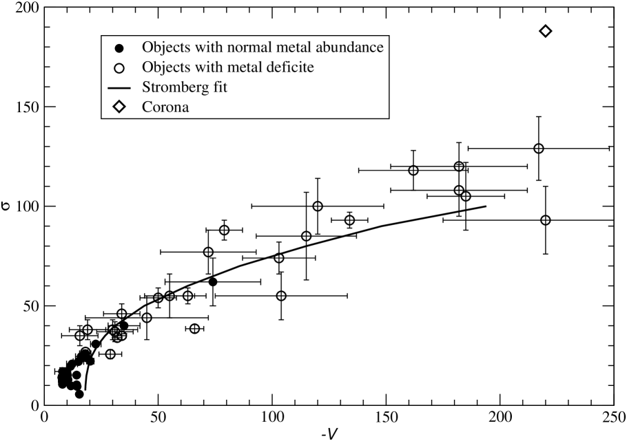
Figure 4: Strömberg diagram for galactic populations according to data presented in Chapter 4. Kinematical data for the corona are taken from the model by Einasto (1979). The Strömberg fit was taken from original Russian version of Chapter 4, it does not take into account the non-stationary status of very young populations.

Physical and kinematical properties of stellar populations depend almost continuously on the age of the population, see Fig. 1. The continuity of stellar populations of various age is reflected also in their kinematical characteristics, such as the velocity dispersion and the heliocentric centroid velocity, expressed in the Strömberg diagram. The oldest halo populations have the lowest metallicity and $M/L$-ratio, see Table LABEL:Tab20.2 and Fig 5, the highest velocity dispersion, and the largest (negative) heliocentric velocity, see Fig. 1 and 4. There is no place to put the new population into this sequence. The dark population is almost spherical and non-rotating. It has a much larger radius than all known stellar populations. In order to be in equilibrium in the Galactic gravitational potential, these coronal stars must have a high velocity dispersion, about $\sigma\approx 200$ km/s, much more than all known stellar populations, up to 125 km/s, see Figs. 1, 1 and 4. Jaaniste & Saar (1975) investigated the possible stellar nature of the corona. Authors found no fast moving stars, possible candidates for coronal objects.

The $M/L$ value, and the spatial and kinematical distribution of the dark population differ greatly from respective properties of all known stellar populations, and there are no intermediate populations. Thus, the corona must have been formed much earlier than all known populations to form the gap in relations between various physical, kinematical and spatial structure parameters. The total mass of the new population exceeds the masses of known populations by an order of magnitude, thus we have a problem: How to transform at an early stage of the evolution of the Universe most of the primordial matter into invisible stars? It is known that star formation is a very inefficient process: in a star-forming gaseous nebula only about 1 % of matter transforms into stars.

As discussed above, neither neutral nor hot ionised gas is a suitable candidate for dark matter. Thus, the nature of coronas remained unclear. It was only much later that the non-baryonic nature of dark matter became evident, as discussed in a conference in Tallinn, April 7 – 10, 1981, and in Vatican Study Week, September 28 – October 2, 1981. Leading Soviet physicists and astronomers attended the Tallinn conference. Several talks were devoted to the formation of the structure of the Universe with neutrinos as dark matter (Yakov Zeldovich, Andrei Doroshkevich, Igor Novikov). In the Vatican Study Week neutrinos as dark matter candidates were discussed by Martin Rees, Joe Silk, Jim Gunn and Dennis Sciama. Difficulties of the neutrino-dominated dark matter were evident, and soon the Cold Dark Matter (CDM) was suggested by Bond et al. (1982), Pagels & Primack (1982), Peebles (1982), and Blumenthal et al. (1984).

Table 1: Galactic parameters

Parameter	Unit	Observed	Smoothed	Adopted	Reference
$R_{0}$	kpc	$8.8\pm 0.7$	$8.5\pm 0.3$	8.5	1, 2
$V$	km/sec	$220\pm 10$	$221\pm 5$	225	3
$W$	“	$120\pm 15$	$133\pm 4$	131.8	4
$A$	km/sec/kpc	$16\pm 1$	$15.7\pm 0.4$	15.5	5 - 7
$C$	“	$70\pm 5$		74	14
$\omega$	“	$26\pm 2$	$26.0\pm 0.7$	26.5	8 -10
$k_{z}$		$0.282\pm 0.020$	$0.285\pm 0.008$	0.293	11
$\rho_{0}$	$M_{\odot}$/pc3	$0.1\pm 0.02$		0.097	12, 13

References: 1. Oort & Plaut (1975), 2. Harris (1976), 3. Einasto et al. (1979), 4. Haud (1984), 5. Crampton & Fernie (1969), 6. Balona & Feast (1974), 7. Crampton & Georgelin (1975), 8. Asteriadis (1977), 9. Fricke (1977), 10. Dieckvoss (1978), 11. Einasto (1972c), 12. Jõeveer (1974), 13. Woolley & Stewart (1967), 14. Jõeveer (1974).

Table 2: Parameters of galactic components

Quantity	Unit	Nucleus	Bulge	Halo	Disc	Flat	Corona
$\epsilon$		0.6	0.6	0.3	0.10	0.02	1
$N$		1	1	4	1	0.5	0.5
$a_{0}$	kpc	0.005	0.21	1.9	4.62	6.4	75
$\mathfrak{M}\,$	$10^{10}\,M_{\odot}$	0.009	0.442	1.2	7.68	1.0	110

The presence of massive dark matter coronas influences galactic models. Thus, I continued together with my collaborators Urmas Haud and Ants Kaasik to develop new models which included dark coronas. To develop the model of our Galaxy, a system of galactic parameters is needed. One of important parameters is the circular velocity near the Sun. Using the method described in Chapter 7 and shown in Fig. 1, we found for the circular velocity $V_{0}=220\pm 7$ km/sec (Einasto et al. 1979). This value is lower than our previous estimate, discussed in Chapter 7, due to the addition of dark corona in the new model. The model of the Galaxy was described in the preliminary form by Einasto et al. (1976b) and in a more polished form by Einasto (1979). In this model, we found an improved system of galactic parameters with $R_{0}=8.5$ kpc, presented in Table 1. Parameters of galactic populations according to this model are given in Table 2. For disc and flat populations parameters are given for positive mass components.

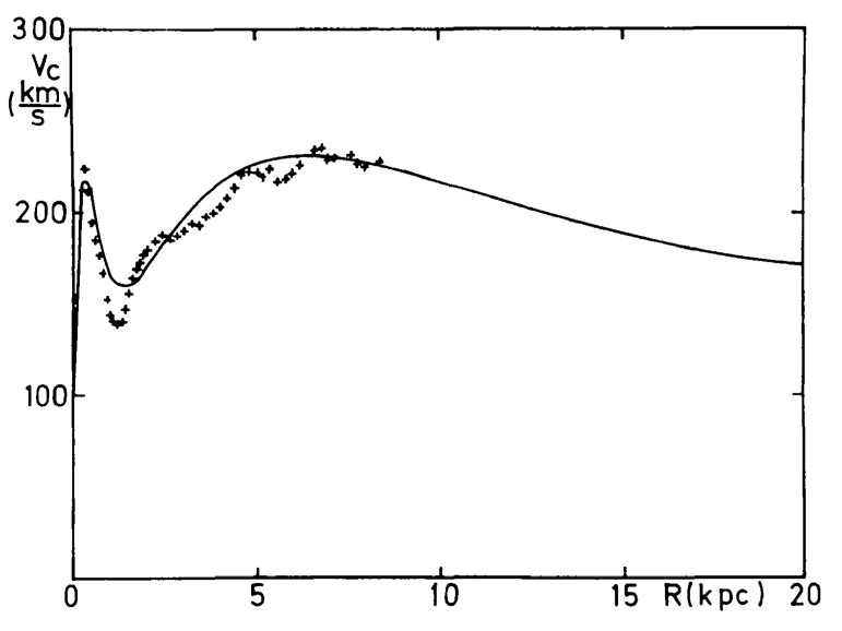
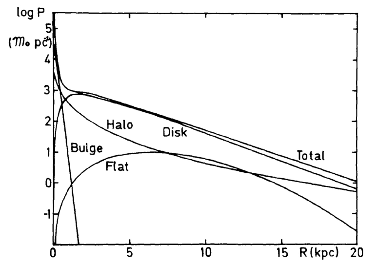
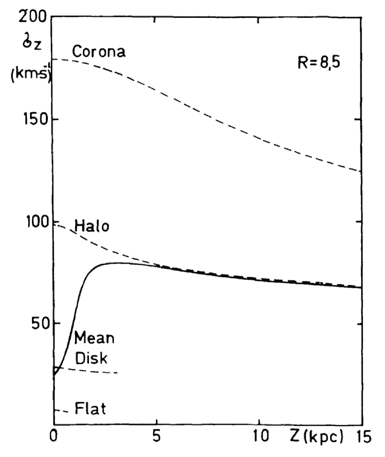
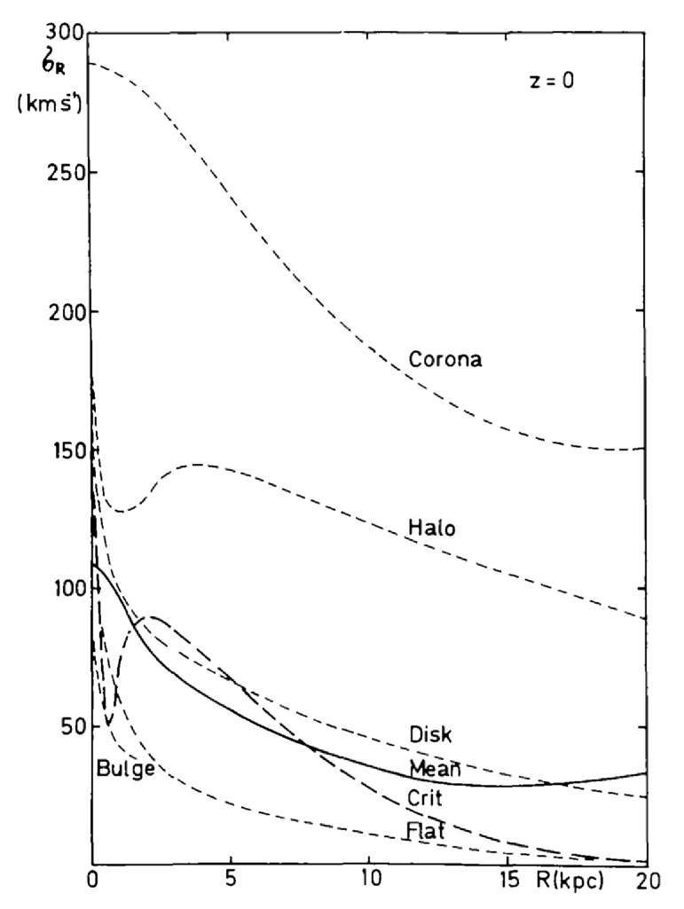
Figure 5: Top panels: Circular velocity surface density of the Galaxy and its components. Bottom panels: Velocity dispersion, $\sigma_{z}$ and $\sigma_{R}$, of galactic populations (Einasto 1979).

In the top left panel of Fig. 5 we show the circular velocity (solid line) and observed rotation velocity (symbols) of the model by Einasto (1979). In the right panel of the Figure we give the surface density of the Galaxy and its components of the same model. In the bottom left panel of Fig. 5 we show the velocity dispersion $\sigma_{z}$ as the function of the distance from the galactic plane, and in the right panel the velocity dispersion $\sigma_{R}$ as the function of the distance from galactic centre (Einasto 1979). Data are given for the main populations: flat, bulge, disc, halo and corona. Also we show the mean dispersion, and the critical dispersion by Toomre (1964). We see that the mean velocity dispersion is larger than the critical Toomre dispersion, thus the model is stable against small radial perturbations.

The critical point in model construction is the determination of mass-to-light ratios for individual populations. For the nucleus and core this ratio can be determined from observations by two methods, from spectrophotometric data and from virial theorem. For the halo we can use the value for globular clusters, determined from velocity dispersions. For the disc and bulge we can use the value for open clusters, as found from velocity dispersion, from the rotation velocity at distance from the center where the disc or bulge dominate, and from calculations of the physical evolution of populations. We assume that the bulge and disc have the same chemical composition and mass-to-light ratio as open clusters with similar colour and spectral properties. The dependence of $f_{B}$ of individual galactic populations on the total mass of galaxies is shown in Fig. 6 and on B-V and U-B colours in Fig. 7 (Einasto 1974a).

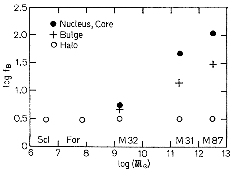
Figure 6: Dependence of mass-to-light ratio $f_{B}$ of old galactic populations on the total mass of galaxies (Einasto 1974a).

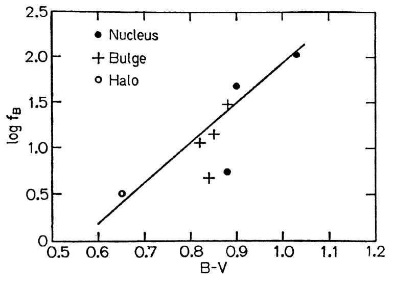
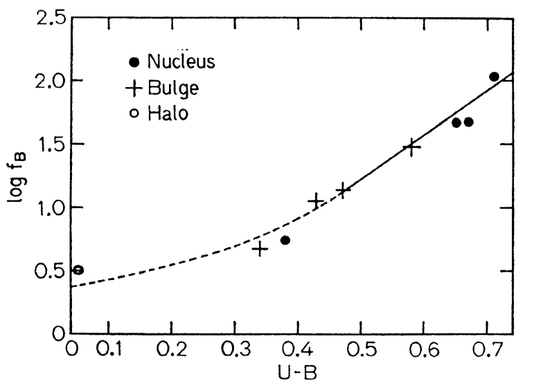
Figure 7: Dependence of mass-to-light ratio $f_{B}$ of old galactic populations on their B-V and U-B colours (Einasto 1974a).

Mass-to-light ratios $f_{B}=M/L_{B}$ of galactic populations are formed during the evolution of stars, and are incorporated in dynamical models of galaxies. $M/L_{B}$-ratios depend on the age and the chemical content of populations, and are fixed by the minimal mass of stars in the star-formation function, $M_{0}$, see Eqs. (2) and (3). I accepted for stellar populations with a normal metal content a lower star formation limit $M_{0}=0.03\leavevmode\nobreak\ M_{\odot}$, for metal-rich populations a limit $M_{0}=0.001\leavevmode\nobreak\ M_{\odot}$, and for metal-poor populations a limit $M_{0}=0.1\leavevmode\nobreak\ M_{\odot}$. Most limits are lower than the lowest masses needed to start hydrogen burning in stars, $M^{\ast}=0.08\leavevmode\nobreak\ M_{\odot}$. Using these lower mass limits, I got for old metal-poor populations $M/L_{B}\leq 3$, for old intermediate populations $M/L_{B}\leq 10$, and for old extremely metal-rich populations $M/L_{B}\leq 100$, see Figs. 5 and 6. The spatial distribution of mass in populations is well determined, and $M/L_{B}$-ratios can be checked by independent velocity dispersion data in small systems of different age and chemical content (open and globular clusters, nuclei of galaxies). As our model calculations showed, it is impossible to reproduce with known populations the observed flat rotation curves of spiral galaxies. In contrast, models based on rotation velocities (Schmidt (1957b), Brandt & Scheer (1965), Roberts (1966), Rubin & Ford (1970)) have a very rapid increase of $M/L_{B}$-ratios on the periphery of M31, see Fig. 6. But these models contain no hint to understand how to explain this increase.

During one of 1976 IAU General Assembly meetings, Sandra Faber discussed her recent measurements of spectra of elliptical galaxies (Faber & Jackson 1976). New data suggested that velocity dispersions of the nuclei of elliptical galaxies are much lower than accepted so far, which leads to a considerable decrease of mass-to-light ratios of elliptical galaxies. This suggests that corrections are needed to my previous galaxy evolution models. This can be done by changing the lower mass limit of forming stars, and using for all populations identical lower mass limits, $M_{0}\approx 0.1\leavevmode\nobreak\ M_{\odot}$, which yields lower $M/L$ values for all populations. A very detailed review of masses and mass-to-light ratios of galaxies is given by Faber & Gallagher (1979). Their Table 1 gives $M/L_{B}$ values within Holmberg radius of galaxies with extended rotation curves. These measured mass-to-light values lie in the interval $0.6\leq M/L_{B}\leq 12$, with a mean value about 4, which corresponds to the disc of galaxies.

In galactic models, the main task is the determination of parameters of populations. First, a crude preliminary model is calculated, model functions are compared with observed functions, and differences are found. In earlier models a simple trial-and-error procedure was applied to find proper values of population parameters. In late 1970s, Urmas Haud suggested applying an automatic procedure for model parameters search. As in previous model calculations, first preliminary values of model parameters are selected, model functions are calculated and compared with observed functions. To estimate the degree of consistence of the model with observational data, the sum of squares of relative deviations is calculated. Next, each model parameter was changed by a small correction, the degree of consistency was found, and a new model was calculated. This procedure was made for all model parameters, one at a time. In this way, optimal values of all model parameters were found. The iterations were completed when the change of an arbitrary parameter by 1 percent did not reduce the sum of the squares of relative deviations. The development of the iteration program demanded much effort and time, thus the method was published only in late 1980s by Einasto & Haud (1989). With this method, first a new model of the Galaxy was found by Haud & Einasto (1989), models of other galaxies were published by Tenjes et al. (1991, 1994, 1998).

We show in Table 3 parameters of components of the model of M31 by Tenjes et al. (1994), and in Fig 8 rotation and mass-to-light curves according to the model. Parameters for the disc and flat subsystems are for positive mass components. In new models the most essential change in comparison with earlier models is the decrease of masses and mass-to-light ratios of the nucleus, core and bulge, and the addition of a massive corona.

Table 3: Parameters of components of M31

Quantity	Unit	Nucleus	Core	Bulge	Halo	Disc	Flat	Corona
$\epsilon$		0.69	0.82	0.67	0.47	0.10	0.02	1
$N$		1.2	1.5	2.4	4.9	1.3	0.3
$a_{0}$	kpc	0.0039	0.10	0.75	4.8	4.1	11.1	60
$\mathfrak{M}\,$	$10^{10}\,M_{\odot}$	0.031	0.20	1.0	0.8	8.4	0.75	320
$f_{B}$	$M_{\odot}/L_{\odot}$	32	13	2.6	2.0	15	1.1
$U-B$		0.88	0.80	0.54	0.21	0.90	$-0.38$
$B-V$			1.03	0.97	0.79	1.01	0.45

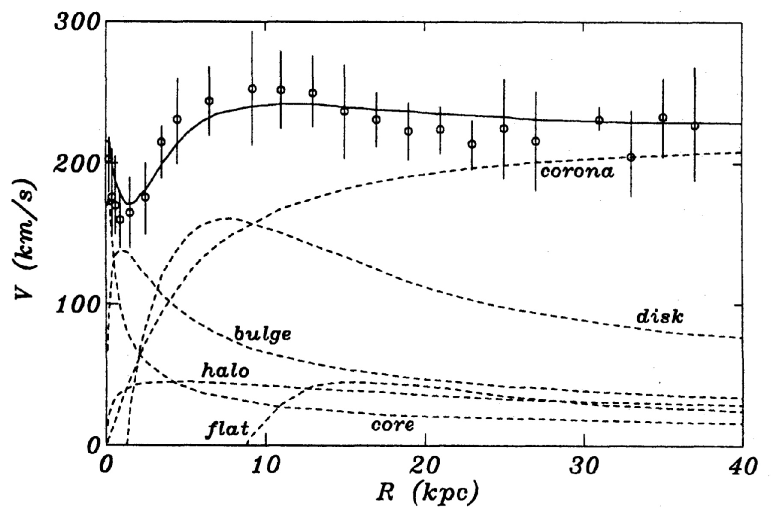
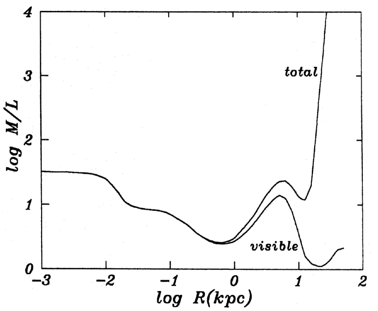
Figure 8: Left:. The rotation curve of M31 according to the model by Tenjes et al. (1994). Open circles – observations, thick line – model, dashed lines – model curves of components. Right: Local mass-to-light ratios for visible populations and for the model with dark corona.

In the case of the M31 model the decrease of masses and mass-to-light ratios reduces the height of the peak of the model circular velocity at small distances from the center, and the addition of the corona improves the model circular velocity on large distance from the center. These changes are well seen when we compare Fig. 3 variant B, Fig. 5 and Fig. 7, and Tables LABEL:Tab17.1 and LABEL:Tab20.2 of previous models with respective data in the new model, presented in Fig. 8 and Table 3.

In galactic models, we used the modified exponential model, Eq. (10), with a parameter $x_{0}$ to improve the shape of the density profile near the centre. This automatic model parameter search showed that for all stellar populations the optimal value of the parameter is $x_{0}=0$. In other words, there is no need for this modification of the exponential profile. Presently this profile is called “Einasto profile”, and is used mainly to describe the spatial density distribution of dark matter halos (Merritt et al. 2005).

The study of the morphology of satellite galaxies was our first step in the investigation of the environment of galaxies. Following a suggestion by Iosif Shklovsky we studied the dynamics of the Magellanic Stream, discovered by Mathewson et al. (1974). The Magellanic Stream is a huge strip of gas through Magellanic Clouds. We noticed that most companions of the Galaxy, including Magellanic Clouds, the Magellanic Stream, and an another stream of high-velocity hydrogen clouds lie close to a plane that is almost perpendicular to the Galactic plane (Einasto et al. 1976a). In this paper we used velocities of satellite galaxies and Magellanic Stream gas clouds to determine the mass of the Galaxy together with its satellites – our Local Hypergalaxy: $M_{tot}=1.2\pm 0.5\times 10^{12}\,M_{\odot}$. Inspired by this pioneering work Urmas Haud continued the study of the dynamics of high-velocity hydrogen clouds surrounding the Galaxy.

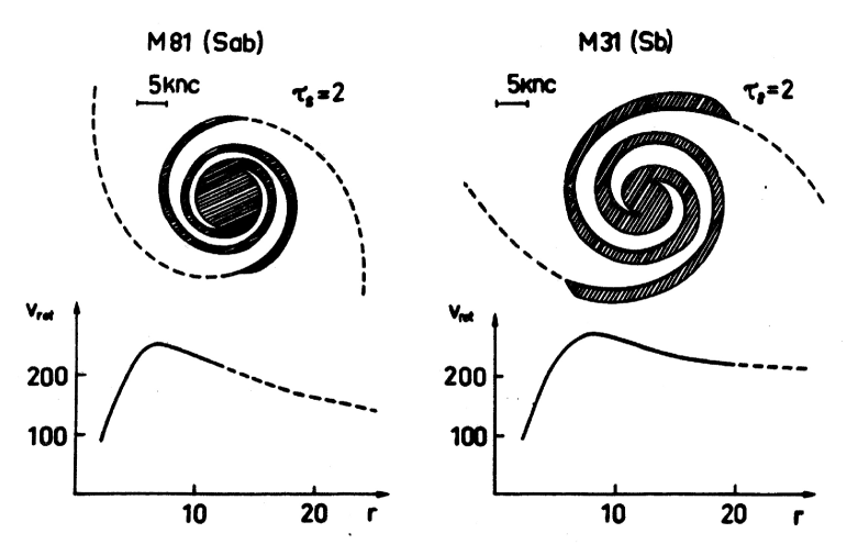
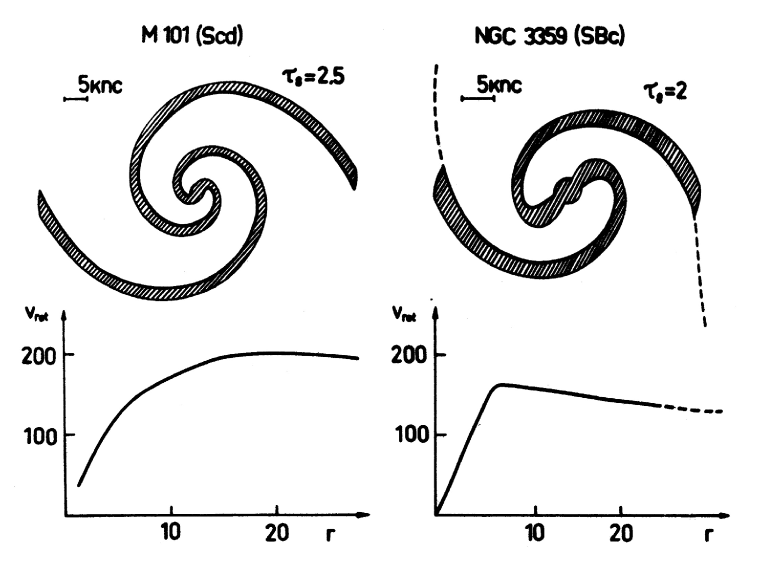
Figure 9: The spiral pattern of four galaxies according to Jaaniste & Saar (1976). Bold lines indicate the loci of new-born stars. The thickness of spiral arms (shaded areas) is determined by the lifetime of massive stars. Dotted curves are hydrogen spiral arms.

Another inspiration suggested by the Magellanic Stream phenomenon concerns the formation of spiral structure of galaxies. Jaaniste & Saar (1976) and Einasto et al. (1976b) noticed that in many giant galaxies dwarf satellite companions are located close to planes perpendicular to the main plane of the central giant galaxy. It is natural to assume that similar to the Magellanic Stream also other giant galaxies have gaseous streams surrounding the main galaxy near the plane of satellites. Gas in these streams falls to the central galaxy along the intersection of planes of the main galaxy and its satellites. These streams initiate perturbations in the gas of the central galaxy and give rise to star formation. Due to the rotation of central galaxies star forming regions form a spiral pattern. Jaaniste & Saar (1976) suggested that the accretion of gas can be the main physical mechanism in the formation of spiral structure of galaxies. Using observed rotation curves of several galaxies authors calculated the expected form of spiral pattern. Results are close to actually observed spiral pattern of galaxies, see Fig. 9.

The study of the environment of galaxies was actually only an introduction to a much wider research area — the distribution of galaxies on large scales. Our involvement in these studies was emphasised by Yakov Zeldovich. After my report on dark matter in galaxies in the Terskol winter school he turned to me and asked to collaborate with him in the study of the Universe. He was developing a theory for the formation of galaxies (Zeldovich 1970), alternative theories were suggested by Peebles & Yu (1970) and Ozernoi (1974), and he was interested to find some observational evidence that can be used to discriminate between these theories.

Initially, we did not know how we can contribute to the problem of galaxy formation. The expected consequences of the Zeldovich model were discussed by Doroshkevich et al. (1974) in the IAU Cosmology Symposium in Krakow 1973. According to this scenario, the first forming objects are superclusters of galaxies which fragment into galaxies. The Peebles & Yu (1970) scenario suggests that the first forming objects are small systems (galaxies or even star clusters), which by gravitational clustering form superclusters of galaxies. Ozernoi (1974) model did not predict any spatial distribution of galaxies. When discussing the problem with my Tartu collaborators, I remembered my previous experience in the study of galactic populations: kinematical and structural properties of galactic populations evolve only slowly, and thus remember their previous state. Large aggregates of galaxies remember their history better, since the crossing time in these systems is larger. Thus we had a leading idea for the search — we have to search for regularities in the large-scale distribution of galaxies.

In this way, we started to collect data on spatial distribution of galaxies in the nearby Universe. This resulted in the discovery of the cosmic web by Jõeveer et al. (1977), Jõeveer & Einasto (1978) and Jõeveer et al. (1978). The observed pattern of the distribution of galaxies has some similarity with the expected distribution, as found with numerical experiments by Doroshkevich & Shandarin (1977). Following this similarity, we called the observed distribution as “cellular”. Subsequently we used the term “supercluster-void network” (Einasto et al. 1980a). Presently the structure is called “cosmic web”, following a suggestion by Bond et al. (1996).

The development of our understanding of the structure and evolution of the Universe is described in detail by Einasto (2014, 2018). This forms a natural extension to my earlier studies on the structure and evolution of galaxies.

November 2021

Chapter B.2 Conclusions

In this Thesis, I have combined three previously independent areas of research in astronomy into one frame: kinematics and spatial properties of Galaxy populations, development of dynamical models of galaxies, and the study of the physical evolution of galaxies. The main results of the study can be divided into methodical and astronomical.

A. Methods of practical stellar dynamics

1. A method has been developed to use tangential velocities to determine kinematical parameters of star samples (Chapter 1 (Einasto 1954)).

2. A method has been developed to determine the mean velocity dispersion of samples of star using radial, tangential or spatial velocities, taking into account observational errors (Chapter 2 (Einasto 1955a)).

3. The concept of the system of galactic parameters has been elaborated, and a method to find the system developed (Chapters 3, 5, 6 (Einasto 1961; Einasto & Kutuzov 1964a; Einasto 1964; Einasto & Kutuzov 1964b)).

4. A method has been developed to extrapolate the mass distribution function beyond the Sun’s distance, and to determine the circular velocity at the Sun’s distance from the Galactic centre (Chapter 7 (Einasto 1965)).

5. The method to construct mass distribution models of galaxies is refined (Chapter 7 (Einasto 1965)).

6. A classification of models of stellar systems, and conditions of physical correctness of models are developed (Chapters 8 and 13 (Einasto 1969a; Kutuzov & Einasto 1968)).

7. A method has been developed to construct spatial and hydrodynamical models of stellar systems (Chapters 10, 11 (Einasto 1968d, 1970c)).

8. The virial theorem has been modified to apply it to components of galaxies (Chapter 12).

9. It is shown that most models of stellar systems are particular cases of two model families: polynomial and binomial models (Chapters 13—15 (Einasto 1968b, c, d)).

10. The generalised exponential model is suggested, and its descriptive functions are determined (Chapters 7, 16 (Einasto 1965; Einasto & Einasto 1972b)).

11. Methods to analyse radio observations are refined to determine density and velocity fields of galaxies (Chapter 19 (Einasto & Rümmel 1970a, c)).

12. The method to reconstruct the dynamical evolution of galaxies on the basis of the structure and kinematics of star populations of different ages is refined (Chapter 21).

13. The method to investigate the physical evolution of galaxies is refined (Chapter 22).

14. A method has been developed to determine parameters of star formation function (Chapter 23 (Einasto 1972d)).

B. The study of the structure and evolution of regular galaxies

1. It is demonstrated that samples of stars of the main sequence later than F spectral class are kinematically heterogeneous (Chapter 1 (Einasto 1954)).

2. The relationship between kinematical characteristics and ages of stellar populations is found (Chapters 3, 4 (Einasto 1954, 1955b)).

3. A new system of galactic parameters is found (Chapters 5, 7 (Einasto & Kutuzov 1964a; Einasto 1964; Einasto & Kutuzov 1964b; Einasto 1965)).

4. Models of the Galaxy are critically analysed and new models are suggested in two approximations (Chapters 5, 7 (Einasto 1965, 1969a, 1970a)).

5. The kinematical and spatial structure of the Andromeda galaxy M31 is studied and its spatial and hydrodynamical models developed in two approximations (Chapters 17 – 20 (Einasto 1969b; Einasto & Rümmel 1970b; Einasto 1972b; Einasto & Rümmel 1972)).

6. The dynamical evolution of the Galaxy is reconstructed using kinematical characteristics of stellar populations of different ages (Chapter 21).

7. On the basis of stellar evolutionary tracks and star formation function, a theory of the evolution of galaxies is elaborated (Chapter 22).

8. Parameters of star formation function are refined (Chapter 23 (Einasto 1972d)).

Results obtained in this series of studies and incorporated in the Thesis were discussed in astronomical seminars in Tartu Observatory, Leningrad State University, Sternberg Astronomical Institute, and in conferences and symposia in Alma-Ata, in IAU General Assembly in Hamburg 1964 (Einasto & Kutuzov 1964a; Einasto 1964; Einasto & Kutuzov 1964b) and in Brighton 1970 (Einasto 1970a, b), in IAU Symposium on Spiral Structure of Our Galaxy in Basel 1969 (Einasto & Rümmel 1970a, c), and in IAU Symposium on External Galaxies and Quasi Stellar Objects in Uppsala 1972 (Einasto 1972b).

November 1971

Chapter C.3 Acknowledgements

First of all I would like to thank my mentors Professors Taavet Rootsmäe, Ernst Öpik, Aksel Kipper and Grigori Kuzmin. Professors Rootsmäe and Kipper created a very high moral and ethical atmosphere in Tartu Observatory. Prof. Rootsmäe’s moto was “Science is carried by the search for truth that is as sincere and honest as Nature itself”, and Prof. Kipper emphasised, “Let a hundred flowers bloom, for we cannot foresee, which blossom will come to bear the best fruit.” Grigori Kuzmin was a student of Ernst Öpik and advised me on how to solve a new problem. First, the problem must be simplified so that only the main factors are taken into account. On the basis of this, one can find a preliminary answer. Thereafter, other factors influencing the process under study can be taken into account, step by step. This allows one to select all important factors and eliminate less important ones. Fritz Zwicky called this approach to solve scientific problems as “morphological”. I tried to follow this experience in my studies. When starting a new program, I first tried to find the answer myself and only later looked at what others have done in the respective area. This helped me to have a fresh outlook on a problem and avoid errors made by earlier investigators.

I am also very grateful to Grigori Kuzmin for his advice on improving my Thesis manuscript. During the work on these problems, we often had long discussions. He always gave me freedom to think for myself and independently. His role was to help me to find errors in my work and give hints on how to do things better.

My sincere gratitude goes to my colleagues at Tartu Observatory Maret Einasto, Mirt Gramann, Jaak Jaaniste, Mihkel Jõeveer, Urmas Haud, Gert Hütsi, Ants Kaasik, Lev Kofman, Sergei Kutuzov, Lauri-Juhan Liivamägi, Dmitri Pogosyan, Enn Saar, Ivan Suhhonenko, Erik Tago, Antti Tamm, Elmo Tempel, Peeter Tenjes, Peeter Traat and Jaan Vennik for the fruitful collaboration and their contribution to the studies, to Peeter Kalamees, Aivo Kivila, Urve Rümmel, Hilju Silvet and Margus Sisask for their help in computations and forming manuscripts, to Piret Zettur for scanning the manuscript and producing with OCR software readable text, to Kerli Linnat for proofreading the English version of the Thesis, and to Marja-Liisa Plats for help in preparing the text for printing.

During the study I had contacts with astronomers in other centres within Soviet Union — Viktor Ambartsumian, Arthur Chernin, Igor Karachentsev, Evgeny Kharadze, Andrei Linde, Kirill Ogorodnikov, Pavel Parenago, Josif Shklovsky, Alexei Starobinsky, and many others. In later years I collaborated closely with Yakov Zeldovich and his team of young physicists Andrei Doroshkevich, Anatoly Klypin, Sergei Shandarin, Rashid Sunyaev and Alexei Starobinsky. Yakov Zeldovich insisted that in solving problems, attention is to be given to essential factors, and when results are available, they must be promptly published. He also emphasised that major results must be published in major journals. He was interested in the nature of phenomena and was quick to change his opinion, if new data suggested a revision. In a conference in Tallinn in April 1981, the non-baryonic nature of dark matter was suggested, and at the conference banquet Zeldovich gave an enthusiastic speech: Observers work hard in sleepless nights to collect data; theorists interpret observations, are often in error, correct their errors and try again; and there are only very rare moments of clarification. Today it is one of such rare moments when we have a holy feeling of understanding secrets of Nature.

I benefitted from contacts with astronomers from other countries. These contacts started already during the Soviet period of my life by visiting conferences and exchanging letters, and continued after the independence of Estonia was restored. Most contacts started after the Thesis was finished and our Tartu team was involved in the study of dark matter and cosmic web. I had discussions with George Abell, Heinz Andernach, Neta and John Bahcall, Ed Bertschinger, Peter Brosche, Margaret and Geoffrey Burbidge, George Contopoulos, Gerard de Vaucouleurs, Tim de Zeeuw, Sandy Faber, Margaret Geller, Wilhelm Gliese, John Huchra, Bernard Jones, Rocky Kolb, Dave Latham, Donald Lynden-Bell, Vicent Martinez, Dick Miller, Volker Müller, Jan Henrik Oort, Jerry Ostriker, Changbom Park, Jim Peebles, Luboŝ Perek, Joel Primack, Martin Rees, Mort Roberts, Vera Rubin, Remo Ruffini, Hyron Spinrad, Alex Szalay, Gustav Andreas Tammann, Beatrice Tinsley, Alar Toomre, Virginia Trimble, Sidney van den Bergh, Rien van de Weygaert, Simon White, and many others. My sincere thanks to all my friends and colleagues — interactions with them helped to develop the present concept of the structure of the universe.

I thank Dr. Tiiu Kaasik and Prof. Toomas Asser who helped me to stay fit and in good health.

My special thanks goes to my wife Liia, both for her participation in the early stages of the research and for her support and understanding during our common life for more than 50 years. I am very grateful to my daughter Maret and grandchildren Peeter, Triin and Stiina for their help in many ways.

I acknowledge the financial support by the Estonian Science Foundation and the Estonian Ministry of Education and the European Regional Development Fund (TK133).

References

- Abell & Eastmond (1968) Abell, G. O. & Eastmond, S. 1968, Luminosity Function of the Elliptical Galaxies in the Virgo Cluster and the Hubble Constant., The Astronomical Journal Supplement, 73, 161
- Agekyan & Baranov (1969) Agekyan, T. A. & Baranov, A. S. 1969, Construction of models of stellar systems by a numerical method., Astrofizika, 5, 305
- Agekyan & Klosovskaya (1962) Agekyan, T. A. & Klosovskaya, E. 1962, Vestnik Leningrad Univ. Math. Mech. Astr. Series, 13
- Aizenman et al. (1969) Aizenman, M. L., Demarque, P., & Miller, R. H. 1969, ON the Interpretation of the Color-Magnitude Diagrams of M67 and NGC 188, ApJ, 155, 973
- Alexander (1958) Alexander, J. B. 1958, The velocity ellipsoid of Ao stars, MNRAS, 118, 161
- Alexander (1967) Alexander, J. B. 1967, The chemical composition and ultra-violet excess of G dwarfs, MNRAS, 137, 41
- Ambartsumian (1968) Ambartsumian, V. A. 1968, Problemy evoliutsii Vselennoi.
- Argyle (1965) Argyle, E. 1965, A Spectrometer Survey of Atomic Hydrogen in the Andromeda Nebula., ApJ, 141, 750
- Arp (1964a) Arp, H. 1964a, The role of the Magellanic Clouds in the understanding of galaxies, in The Galaxy and the Magellanic Clouds, ed. F. J. Kerr, 219
- Arp (1964b) Arp, H. 1964b, Spiral Structure in M31., ApJ, 139, 1045
- Arp (1965) Arp, H. 1965, Properties of the Galactic Nucleus in the Direction of NGC 6522., ApJ, 141, 43
- Arp (1966) Arp, H. 1966, Atlas of Peculiar Galaxies, ApJS, 14, 1
- Arp & Bertola (1971) Arp, H. & Bertola, F. 1971, Faint Outer Regions of Elliptical Galaxies, ApJ, 163, 195
- Arp et al. (1963) Arp, H., Brueckel, F., & Lourens, J. V. B. 1963, Long-Period and Red Variables in 47 Tucanae., ApJ, 137, 228
- Asteriadis (1977) Asteriadis, G. 1977, Determination of Precession and Galactic Rotation from the Proper Motions of the AGK3, A&A, 56, 25
- Baade (1951) Baade, W. 1951, Galaxies - Present Day Problems, in Michigan Symposium on Astrophysics, Vol. 10, 24
- Baade (1958) Baade, W. 1958, The Population of the Galactic Nucleus and the Evidence for the Presence of an Old Population Pervading the Whole Disk of our Galaxy, Ricerche Astronomiche, 5, 303
- Baade & Arp (1964) Baade, W. & Arp, H. 1964, Positions of Emission Nebulae in M31., ApJ, 139, 1027
- Baade & Gaposchkin (1963) Baade, W. & Gaposchkin, C. H. P. 1963, Evolution of stars and galaxies. (Cambridge, Harvard University Press 1963)
- Baade & Swope (1963) Baade, W. & Swope, H. H. 1963, Variable star field 96’ south preceeding the nucleous of the Andromeda galaxy., AJ, 68, 435
- Babcock (1939) Babcock, H. W. 1939, The rotation of the Andromeda Nebula, Lick Observatory Bulletin, 498, 41
- Balona & Feast (1974) Balona, L. A. & Feast, M. W. 1974, A new determination from OB stars of the galactic rotation constants and the distance to the galactic centre., MNRAS, 167, 621
- Becker (1970) Becker, W. 1970, The Spiral Structure of our Galaxy, ed. G. C. W. Becker (Reidel Publ.)
- Blaauw (1952) Blaauw, A. 1952, The velocity distribution of the interstellar calcium clouds, Bull. Astron. Inst. Netherlands, 11, 459
- Blaauw & Schmidt (1965) Blaauw, A. & Schmidt, M. 1965, Galactic structure, Vol. 5 (Univ. Chicago Press)
- Blumenthal et al. (1984) Blumenthal, G. R., Faber, S. M., Primack, J. R., & Rees, M. J. 1984, Formation of galaxies and large-scale structure with cold dark matter, Nature, 311, 517
- Bond et al. (1996) Bond, J. R., Kofman, L., & Pogosyan, D. 1996, How filaments of galaxies are woven into the cosmic web, Nature, 380, 603
- Bond et al. (1982) Bond, J. R., Szalay, A. S., & Turner, M. S. 1982, Formation of galaxies in a gravitino-dominated universe, Physical Review Letters, 48, 1636
- Bosma (1978) Bosma, A. 1978, The distribution and kinematics of neutral hydrogen in spiral galaxies of various morphological types, PhD thesis, Groningen Univ.
- Bottlinger (1933) Bottlinger, K. F. 1933, Beitraege zur Theorie der Rotation des Sternsystems, Veroeffentlichungen der Universitaetssternwarte zu Berlin-Babelsberg, 2
- Brandt (1960) Brandt, J. C. 1960, On the Distribution of Mass in Galaxies. I. The Large-Scale Structure of Ordinary Spirals with Applications to M 31, ApJ, 131, 293
- Brandt & Roosen (1969) Brandt, J. C. & Roosen, R. G. 1969, Messier 87: the Galaxy of Greatest Known Mass, ApJ, 156, L59
- Brandt & Scheer (1965) Brandt, J. C. & Scheer, L. S. 1965, A note on functions relating to galactic structure, AJ, 70, 471
- Brosche (1970) Brosche, P. 1970, A Model for the Early Evolution of Galaxies, A&A, 6, 240
- Burbidge et al. (1957) Burbidge, E. M., Burbidge, G. R., Fowler, W. A., & Hoyle, F. 1957, Synthesis of the Elements in Stars, Reviews of Modern Physics, 29, 547
- Burbidge et al. (1959) Burbidge, E. M., Burbidge, G. R., & Prendergast, K. H. 1959, The Rotation and Mass of NGC 2146., ApJ, 130, 739
- Burbidge et al. (1960) Burbidge, E. M., Burbidge, G. R., & Prendergast, K. H. 1960, The Rotation, Mass Distribution, and Mass of NGC 5055., ApJ, 131, 282
- Burbidge (1975) Burbidge, G. 1975, On the masses and relative velocities of galaxies, ApJ, 196, L7
- Burke et al. (1963) Burke, B. F., Turner, K. C., & Tuve, M. A. 1963, Hydrogen Motions in M31., AJ, 68, 274
- Cameron & Truran (1971) Cameron, A. G. W. & Truran, J. W. 1971, The Chemical Evolution of the Galaxy, JRASC, 65, 1
- Cannon (1970) Cannon, R. D. 1970, Red giants in old open clusters., MNRAS, 150, 111
- Carranza et al. (1968) Carranza, G., Courtes, G., Georgelin, Y., Monnet, G., & Pourcelot, A. 1968, Interferometric study of ionized hydrogen in M 33. New kinematical and physical data, Annales d’Astrophysique, 31, 63
- Caswell (1970) Caswell, J. L. 1970, The Frequency of Supernovae in our Galaxy, Estimated from Supernova Remnants Detected at 178 MHz, A&A, 7, 59
- Chernin et al. (1976) Chernin, A., Einasto, J., & Saar, E. 1976, The role of diffuse matter in galactic coronas, Ap&SS, 39, 53
- Conti & Strom (1968) Conti, P. S. & Strom, S. E. 1968, The Early a Stars. II. Model-Atmosphere Abundance Analysis of Eight Stars in the Pleiades, ApJ, 152, 483
- Crampin & Hoyle (1964) Crampin, D. J. & Hoyle, F. 1964, On the Angular-Momentum Distribution in the Disks of Spiral Galaxies., ApJ, 140, 99
- Crampton & Fernie (1969) Crampton, D. & Fernie, J. D. 1969, A New Determination of Oort’s Constant A from Cepheids, AJ, 74, 53
- Crampton & Georgelin (1975) Crampton, D. & Georgelin, Y. M. 1975, The distribution of optical H II regions in our Galaxy., A&A, 40, 317
- Cuperman et al. (1969) Cuperman, S., Goldstein, S., & Lecar, M. 1969, Numerical experimental check of Lynden-Bell statistics-II. The core-halo structure and the role of the violent relaxation, MNRAS, 146, 161
- Davies (1969) Davies, R. D. 1969, personal communication
- Davis & Webb (1970) Davis, J. & Webb, R. J. 1970, Ultraviolet Fluxes and Bolometric Corrections for Late B to F Main-Sequence Stars, ApJ, 159, 551
- Day (1969) Day, R. W. 1969, The Solar Motion of AP Stars, PASP, 81, 866
- de Vaucouleurs (1948) de Vaucouleurs, G. 1948, Recherches sur les Nebuleuses Extragalactiques, Annales d’Astrophysique, 11, 247
- de Vaucouleurs (1953) de Vaucouleurs, G. 1953, On the distribution of mass and luminosity in elliptical galaxies, MNRAS, 113, 134
- de Vaucouleurs (1958) de Vaucouleurs, G. 1958, Photoelectric photometry of the Andromeda Nebula in the UBV system., ApJ, 128, 465
- de Vaucouleurs (1959) de Vaucouleurs, G. 1959, Classification and Morphology of External Galaxies., Handbuch der Physik, 53, 275
- de Vaucouleurs (1961) de Vaucouleurs, G. 1961, Integrated Colors of Bright Galaxies in the U, B, V System., ApJS, 5, 233
- de Vaucouleurs (1962) de Vaucouleurs, G. 1962, Problems of Ectra-Galactic Research, ed. G. C. McVittie (MacMillan, New York)
- de Vaucouleurs (1969) de Vaucouleurs, G. 1969, Photometry of the Outer Corona of Messier 87, Astrophys. Letters, 4, 17
- Deharveng & Pellet (1969) Deharveng, J. M. & Pellet, A. 1969, Etude interférometrique des régions H II du bras nord-est de M31., A&A, 1, 208
- Delhaye (1965) Delhaye, J. 1965, Solar Motion and Velocity Distribution of Common Stars, ed. S. M. Blaauw, A. No. 61, 61
- Demarque (1967) Demarque, P. 1967, The Early Evolution of Population II Stars, ApJ, 149, 117
- Demarque et al. (1968) Demarque, P., Hartwick, F. D. A., & Naylor, M. D. T. 1968, Some Uncertainties in Population II Stellar Models Near the Main Sequence, ApJ, 154, 1143
- Demarque & Mengel (1971a) Demarque, P. & Mengel, J. G. 1971a, Advanced Evolution of Population II Stars. I. Red Giants and the Helium Flash, ApJ, 164, 317
- Demarque & Mengel (1971b) Demarque, P. & Mengel, J. G. 1971b, Advanced Evolution of Population II Stars. II. The Horizontal Branch, ApJ, 164, 469
- Demarque et al. (1971) Demarque, P., Mengel, J. G., & Aizenman, M. L. 1971, The Early Evolution of Population II Stars. II, ApJ, 163, 37
- Demarque & Miller (1969) Demarque, P. & Miller, R. H. 1969, On the Color-Magnitude Diagrams of NGC 2360 and NGC 3680, ApJ, 158, 1037
- Demarque & Schlesinger (1969) Demarque, P. & Schlesinger, B. M. 1969, On the Chemical Composition and Age of NGC 188, ApJ, 155, 965
- Dicke (1969) Dicke, R. H. 1969, The Age of the Galaxy from the Decay of Uranium, ApJ, 155, 123
- Dieckvoss (1978) Dieckvoss, W. 1978, Formal values for constants of solar motion and galactic rotation from proper motions., A&A, 62, 445
- Dieter (1969) Dieter, N. H. 1969, High-Velocity Interstellar Gas, PASP, 81, 186
- Dixon (1965) Dixon, M. E. 1965, The two-colour diagram as a key to past rates of star formation and past rates of maetal enrichment of the interstellar medium, MNRAS, 129, 51
- Dixon (1966) Dixon, M. E. 1966, The two colour diagram as a key to past rates of star formation and past rates of metal enrichment of the interstellar medium, II, MNRAS, 131, 325
- Dixon (1967a) Dixon, M. E. 1967a, Spiral arms, MNRAS, 137, 337
- Dixon (1967b) Dixon, M. E. 1967b, The kinematic properties of young stars, AJ, 72, 429
- Dixon (1968) Dixon, M. E. 1968, Interstellar gas dynamics and the motions of young stars, MNRAS, 140, 287
- Doroshkevich & Shandarin (1977) Doroshkevich, A. G. & Shandarin, S. F. 1977, Large-scale distribution and motion of galaxies, AZh, 54, 734
- Doroshkevich et al. (1974) Doroshkevich, A. G., Sunyaev, R. A., & Zeldovich, I. B. 1974, The formation of galaxies in Friedmannian universes, in IAU Symposium, Vol. 63, Confrontation of Cosmological Theories with Observational Data, ed. M. S. Longair, 213
- Doroshkevich et al. (1967) Doroshkevich, A. G., Zeldovich, Y. B., & Novikov, I. D. 1967, The Origin of Galaxies in an Expanding Universe., Soviet Ast., 11, 233
- Dyer (1956) Dyer, Edward R., J. 1956, An analysis of the space motions of red dwarf stars, AJ, 61, 228
- Eddington (1915) Eddington, A. S. 1915, The dynamics of a stellar system. Third paper: oblate and other distributions, MNRAS, 76, 37
- Edmondson (1956) Edmondson, F. K. 1956, The local standard of rest., AJ, 61, 175
- Eelsalu (1958) Eelsalu, H. 1958, The gradient of the gravitational acceleration perpendicular to the Galactic plane near the Sun, Tartu Astr. Obs. Publ., 33, 153
- Eelsalu (1961) Eelsalu, H. 1961, On the reliability of the determination of the gravitational acceleration perpendicular to the Galactic plane, Publications of the Tartu Astrofizica Observatory, 33, 416
- Eggen (1950a) Eggen, O. J. 1950a, Photoelectric Studies. I. Color-Luminosity Array for Members of the Hyades Cluster., ApJ, 111, 65
- Eggen (1950b) Eggen, O. J. 1950b, Photoelectric Studies. II. Color-Luminosity Array for Members of the Pleiades Cluster., ApJ, 111, 81
- Eggen (1950c) Eggen, O. J. 1950c, Photoelectric Studies. III. Color-Luminosity Arrays for the Coma Berenices and Ursa Major Clusters., ApJ, 111, 414
- Eggen (1959) Eggen, O. J. 1959, Motions of the bright peculiar and metallic-line A-type stars, The Observatory, 79, 197
- Eggen (1960a) Eggen, O. J. 1960a, Stellar groups, V. Luminosities, motions and masses of the late-type sub-giants, MNRAS, 120, 430
- Eggen (1960b) Eggen, O. J. 1960b, Stellar groups, VI. Space motions of the dwarf A-type and giant M-type stars in the solar neighbourhood, MNRAS, 120, 448
- Eggen (1962) Eggen, O. J. 1962, Space-velocity vectors for 3483 stars with proper motion and radial velocity., Royal Greenwich Observatory Bulletins, 51, 79
- Eggen (1964) Eggen, O. J. 1964, A catalogue of high-velocity stars, Royal Greenwich Observatory Bulletins, 84, 111
- Eggen (1968) Eggen, O. J. 1968, The Intermediate-Age Cluster NGC 2360, ApJ, 152, 83
- Eggen (1969a) Eggen, O. J. 1969a, The Motions of the A Stars at the North Galactic Pole, PASP, 81, 741
- Eggen (1969b) Eggen, O. J. 1969b, The Old Galactic Cluster NGC 3680, ApJ, 155, 439
- Eggen (1970) Eggen, O. J. 1970, A Very Young Cluster with a Moderate Metal Deficiency, ApJ, 161, 159
- Eggen et al. (1962) Eggen, O. J., Lynden-Bell, D., & Sandage, A. R. 1962, Evidence from the motions of old stars that the Galaxy collapsed, ApJ, 136, 748
- Eggen & Sandage (1964) Eggen, O. J. & Sandage, A. R. 1964, New photoelectric observations of stars in the old galactic cluster M67, ApJ, 140, 130
- Eigenson (1960) Eigenson, M. S. 1960, Vnegalakticheskaia astronomiia.
- Einasto (1952) Einasto, J. 1952, Kinematic division of the main sequence into two populations., Publications of the Tartu Astrofizica Observatory, 32, 231
- Einasto (1954) Einasto, J. 1954, On the kinematic structure of the main sequence., Publications of the Tartu Astrofizica Observatory, 32, 371
- Einasto (1955a) Einasto, J. 1955a, Determination of the velocity dispersion of stars from their radial, tangential and spatial velocities, Publications of the Tartu Astrofizica Observatory, 33, 35
- Einasto (1955b) Einasto, J. 1955b, On the kinematics of Me dwarfs., Publications of the Tartu Astrofizica Observatory, 33, 57
- Einasto (1961) Einasto, J. 1961, On the asymmetric shift of stellar velocity centroids, Publications of the Tartu Astrofizica Observatory, 33, 371
- Einasto (1964) Einasto, J. 1964, The Value of Dynamical Parameter C, Tartu Astrofuusika Observatoorium Teated, 11, 1
- Einasto (1965) Einasto, J. 1965, On the Construction of a Composite Model for the Galaxy and on the Determination of the System of Galactic Parameters, Trudy Astrofizicheskogo Instituta Alma-Ata, 5, 87
- Einasto (1968a) Einasto, J. 1968a, On constructing models of stellar systems. II. The descriptive functions and parameters., Publications of the Tartu Astrofizica Observatory, 36, 357
- Einasto (1968b) Einasto, J. 1968b, On constructing models of stellar systems. IV. The power-polynomial model., Publications of the Tartu Astrofizica Observatory, 36, 396
- Einasto (1968c) Einasto, J. 1968c, On constructing models of stellar systems. V. The binomial model., Publications of the Tartu Astrofizica Observatory, 36, 414
- Einasto (1968d) Einasto, J. 1968d, On constructing models of stellar systems. VI. On the methods of model constructing., Publications of the Tartu Astrofizica Observatory, 36, 442
- Einasto (1969a) Einasto, J. 1969a, On Galactic Descriptive Functions, Astronomische Nachrichten, 291, 97
- Einasto (1969b) Einasto, J. 1969b, The Andromeda galaxy M31. I. A preliminary model, Astrofizika, 5, 137
- Einasto (1970a) Einasto, J. 1970a, On the structure and evolution of the Galaxy., Tartu Astrofuusika Observatoorium Teated, 26, 1
- Einasto (1970b) Einasto, J. 1970b, Structural and kinematical properties of populations of the Andromeda galaxy, Tartu Astrofuusika Observatoorium Teated, 26, 23
- Einasto (1970c) Einasto, J. 1970c, The Andromeda galaxy M31. II. Hydrodynamical model. Theory., Astrofizika, 6, 149
- Einasto (1972a) Einasto, J. 1972a, Galactic Models and Stellar Orbits, Tartu Astrofuusika Observatoorium Teated, 40, 3
- Einasto (1972b) Einasto, J. 1972b, Structural and Kinematic Properties of Populations of the Andromeda Galaxy, in IAU Symposium, Vol. 44, External Galaxies and Quasi-Stellar Objects, ed. D. S. Evans, D. Wills, & B. J. Wills, 37
- Einasto (1972c) Einasto, J. 1972c, Structure and Evolution of Regular Galaxies, Thesis, doctor of science, Tartu University
- Einasto (1972d) Einasto, J. 1972d, The Rate of Star Formation, Astrophys. Letters, 11, 195
- Einasto (1974a) Einasto, J. 1974a, Galactic Models and Stellar Orbits (Invited Lecture), in Stars and the Milky Way System, ed. L. N. Mavridis, 291
- Einasto (1974b) Einasto, J. 1974b, The correlation between kinematical properties and ages of stellar populations., in Kinematics and Ages of Stars Near the Sun, 419
- Einasto (1979) Einasto, J. 1979, Galactic mass modeling, in IAU Symposium, Vol. 84, The Large-Scale Characteristics of the Galaxy, ed. W. B. Burton, 451
- Einasto (2014) Einasto, J. 2014, Dark Matter and Cosmic Web Story, ed. R. Ruffini (World Scientific Publishing Co)
- Einasto (2018) Einasto, J. 2018, Cosmology Paradigm Changes, ARA&A, 56, 1
- Einasto & Einasto (1972a) Einasto, J. & Einasto, L. 1972a, Descriptive functions of the Galaxy., Tartu Astrofuusika Observatoorium Teated, 36, 46
- Einasto & Einasto (1972b) Einasto, J. & Einasto, L. 1972b, Modified exponential models of stellar systems., Tartu Astrofuusika Observatoorium Teated, 36, 3
- Einasto & Haud (1989) Einasto, J. & Haud, U. 1989, Galactic models with massive corona. I - Method. II - Galaxy, A&A, 223, 89
- Einasto et al. (1979) Einasto, J., Haud, U., & Jõeveer, M. 1979, The Galactic Circular Velocity Near the Sun, in The Large-Scale Characteristics of the Galaxy, ed. W. B. Burton, Vol. 84, 231
- Einasto et al. (1976a) Einasto, J., Haud, U., Jõeveer, M., & Kaasik, A. 1976a, The Magellanic Stream and the mass of our hypergalaxy., MNRAS, 177, 357
- Einasto et al. (1976b) Einasto, J., Jõeveer, M., & Kaasik, A. 1976b, The mass of the Galaxy, Tartu Astr. Obs. Teated, 54, 3
- Einasto et al. (1980a) Einasto, J., Jõeveer, M., & Saar, E. 1980a, Superclusters and galaxy formation, Nature, 283, 47
- Einasto et al. (1974a) Einasto, J., Kaasik, A., & Saar, E. 1974a, Dynamic evidence on massive coronas of galaxies, Nature, 250, 309
- Einasto & Kutuzov (1964a) Einasto, J. & Kutuzov, S. A. 1964a, A preliminary system of Galactic parameters, Tartu Astrofuusika Observatoorium Teated, 10, 1
- Einasto & Kutuzov (1964b) Einasto, J. & Kutuzov, S. A. 1964b, On the System of Galactic Parameters, Tartu Astrofuusika Observatoorium Teated, 11, 11
- Einasto & Rümmel (1970a) Einasto, J. & Rümmel, U. 1970a, Density Distribution and the Radial Velocity Field in the Spiral Arms of M31, in The Spiral Structure of our Galaxy, ed. W. Becker & G. I. Kontopoulos, Vol. 38, 42
- Einasto & Rümmel (1970b) Einasto, J. & Rümmel, U. 1970b, The Andromeda Galaxy M31. III. Hydrodynamical model, Astrofizika, 6, 241
- Einasto & Rümmel (1970c) Einasto, J. & Rümmel, U. 1970c, The Rotation Curve, Mass, Light and Velocity Distribution of M31, in The Spiral Structure of our Galaxy, ed. W. Becker & G. I. Kontopoulos, Vol. 38, 51
- Einasto & Rümmel (1972) Einasto, J. & Rümmel, U. 1972, Descriptive functions of the Andromeda galaxy., Tartu Astrofuusika Observatoorium Teated, 36, 55
- Einasto et al. (1974b) Einasto, J., Saar, E., Kaasik, A., & Chernin, A. D. 1974b, Missing mass around galaxies - Morphological evidence, Nature, 252, 111
- Einasto et al. (1980b) Einasto, J., Tenjes, P., Barabanov, A. V., & Zasov, A. V. 1980b, Central Holes in Disks of Spiral Galaxies, Ap&SS, 67, 31
- Faber & Gallagher (1979) Faber, S. M. & Gallagher, J. S. 1979, Masses and mass-to-light ratios of galaxies, ARA&A, 17, 135
- Faber & Jackson (1976) Faber, S. M. & Jackson, R. E. 1976, Velocity dispersions and mass-to-light ratios for elliptical galaxies, ApJ, 204, 668
- Faulkner & Iben (1966) Faulkner, J. & Iben, Icko, J. 1966, The Evolution of Population II Stars, ApJ, 144, 995
- Feast (1963) Feast, M. W. 1963, The long period variables, MNRAS, 125, 367
- Feast & Shuttleworth (1965) Feast, M. W. & Shuttleworth, M. 1965, The kinematics of B stars, cepheids, galactic clusters and interstellar gas in the Galaxy, MNRAS, 130, 243
- Feast & Thackeray (1958) Feast, M. W. & Thackeray, A. D. 1958, Analysis of radial velocities of distant B type stars, MNRAS, 118, 125
- Fitzgerald (1970) Fitzgerald, M. P. 1970, The Intrinsic Colours of Stars and Two-Colour Reddening Lines, A&A, 4, 234
- Fricke (1949a) Fricke, W. 1949a, Die Rotationsgeschwindigkeit der Milchstraße in sonnennähe, Astronomische Nachrichten, 278, 49
- Fricke (1949b) Fricke, W. 1949b, Über den Beitrag der Sterne hoher Geschwindigkeit zur Kinematik des Sternsystems, Astronomische Nachrichten, 277, 241
- Fricke (1954) Fricke, W. 1954, Die Intensitäts-und Farbverteilung in Andromeda-Nebel. Mit 17 Textabbildungen, ZAp, 34, 137
- Fricke (1977) Fricke, W. 1977, Basic Material for the Determination of Precession and of Galactic Rotation and a Review of Methods and Results, Veroeffentlichungen des Astronomischen Rechen-Instituts Heidelberg, 28, 1
- Gascoigne & Eggen (1957) Gascoigne, S. C. B. & Eggen, O. J. 1957, Cepheid variables and galactic absorption, MNRAS, 117, 430
- Gilmore et al. (1989) Gilmore, G., Wyse, R. F. G., & Kuijken, K. 1989, Kinematics, chemistry, and structure of the Galaxy, ARA&A, 27, 555
- Gliese (1958) Gliese, W. 1958, Die Geschwindigkeitsverteilung der M-Zwerge mit Emissionslinien, ZAp, 45, 293
- Goldstein et al. (1969) Goldstein, S., Cuperman, S., & Lecar, M. 1969, Numerical experimental check of Lynden-Bell statistics for a collisionless one-dimensional stellar system, MNRAS, 143, 209
- Gottesman et al. (1966) Gottesman, S. T., Davies, R. D., & Reddish, V. C. 1966, A neutral hydrogen survey of the southern regions of the Andromeda nebula, MNRAS, 133, 359
- Gray (1965) Gray, D. F. 1965, Integrated colors and magnitudes of open clusters., AJ, 70, 362
- Greenstein et al. (1970) Greenstein, J. L., Neugebauer, G., & Becklin, E. E. 1970, The Faint End of the Main Sequence, ApJ, 161, 519
- Grossman (1970) Grossman, A. S. 1970, Evolution of Low-Mass Stars. I. Contraction to the Main Sequence, ApJ, 161, 619
- Grossman & Graboske (1971) Grossman, A. S. & Graboske, H. C., J. 1971, Evolution of Low-Mass Stars. III. Effects of Nonideal Thermodynamic Properties during the Pre-Main Contraction, ApJ, 164, 475
- Grossman et al. (1970) Grossman, A. S., Mutschlecner, J. P., & Pauls, T. A. 1970, Evolution of Low-Mass Stars. II. Effects of Primordial Deuterium Burning and a Nongray Surface Condition during Pre-Main Sequence Contraction, ApJ, 162, 613
- Gunn & Kraft (1963) Gunn, J. E. & Kraft, R. P. 1963, An Analysis Abundance of Two F-Type Stars in the Galactic Cluster NGC 752., ApJ, 137, 301
- Gurevich (1964) Gurevich, L. E. 1964, Evolution of Stellar Systems, Problems of Cosmogeny, 2, 158
- Hanbury Brown et al. (1967) Hanbury Brown, R., Davis, J., Allen, L. R., & Rome, J. M. 1967, The stellar interferometer at Narrabri Observatory-II. The angular diameters of 15 stars, MNRAS, 137, 393
- Haro (1950) Haro, G. 1950, Hce emission objects in M 31 and M 33, AJ, 55, 66
- Harris (1976) Harris, W. E. 1976, Spatial structure of the globular cluster system and the distance to the galactic center., AJ, 81, 1095
- Hartwick (1971) Hartwick, F. D. A. 1971, On the Rate of Star Formation in M31, ApJ, 163, 431
- Haud (1984) Haud, U. 1984, Rotation curve of our Galaxy for R>R o, Ap&SS, 104, 337
- Haud & Einasto (1989) Haud, U. & Einasto, J. 1989, Galactic Models with Massive Corona - Part Two - Galaxy, A&A, 223, 95
- Hayashi et al. (1962) Hayashi, C., Hōshi, R., & Sugimoto, D. 1962, Evolution of the Stars, Progress of Theoretical Physics Supplement, 22, 1
- Hayashi & Nakano (1963) Hayashi, C. & Nakano, T. 1963, Evolution of Stars of Small Masses in the Pre-Main-Sequence Stages, Progress of Theoretical Physics, 30, 460
- Helfer et al. (1959) Helfer, H. L., Wallerstein, G., & Greenstein, J. L. 1959, Abundances in Some Population II K Giants., ApJ, 129, 700
- Henon (1969) Henon, M. 1969, Numerical exploration of the restricted problem, V, A&A, 1, 223
- Hindman (1967) Hindman, J. V. 1967, A high resolution study of the distribution and motions of neutral hydrogen in the Small Cloud of Magellan, Australian Journal of Physics, 20, 147
- Hins & Blaauw (1948) Hins, C. H. & Blaauw, A. 1948, Star streaming among faint low-latitude stars investigated according to the dispersion method, Bull. Astron. Inst. Netherlands, 10, 365
- Hohenberg (1969) Hohenberg, C. M. 1969, Radioisotopes and the History of Nucleosynthesis in the Galaxy, Science, 166, 212
- Hohl & Campbell (1968) Hohl, F. & Campbell, J. W. 1968, Statistical Mechanics of a Collisionless Self-Gravitating System, AJ, 73, 611
- Hohl & Feix (1968) Hohl, F. & Feix, M. R. 1968, A Variational Principle for a One-Dimensional Stellar System, ApJ, 151, 783
- Holmberg (1937) Holmberg, E. 1937, A study of double and multiple galaxies, Annals of the Observatory of Lund, 6, 1
- Holmberg (1964) Holmberg, E. 1964, Meddelanden fran Astronomiska Observatorium Uppsala, 148, 1
- Holmberg (1969) Holmberg, E. 1969, A study of physical groups of galaxies, Arkiv for Astronomi, 5, 305
- Hoyle & Schwarzschild (1955) Hoyle, F. & Schwarzschild, M. 1955, On the Evolution of Type II Stars., ApJS, 2, 1
- Hubble (1930) Hubble, E. P. 1930, Distribution of luminosity in elliptical nebulae., ApJ, 71, 231
- Iben (1965a) Iben, Icko, J. 1965a, Stellar Evolution. I. The Approach to the Main Sequence., ApJ, 141, 993
- Iben (1965b) Iben, Icko, J. 1965b, Stellar Evolution. II. The Evolution of a 3 M_{sun} Star from the Main Sequence Through Core Helium Burning., ApJ, 142, 1447
- Iben (1966a) Iben, Icko, J. 1966a, Stellar Evolution. III. The Evolution of a 5 M_{sun} Star from the Main Sequence Through Core Helium Burning, ApJ, 143, 483
- Iben (1966b) Iben, Icko, J. 1966b, Stellar Evolution. V. The Evolution of a 15 M_{sun} Star from the Main Sequence Through Core Helium, ApJ, 143, 516
- Iben (1966c) Iben, Icko, J. 1966c, Stellar Evolution.IV. The Evolution of a 9 M_{sun} Star from the Main Sequence Through Core Helium Burning, ApJ, 143, 505
- Iben (1967a) Iben, Icko, J. 1967a, Stellar Evolution. VII. The Evolution of a 2.25 M_{sun} Star from the Main Sequence to the Helium-Burning Phase, ApJ, 147, 650
- Iben (1967b) Iben, Icko, J. 1967b, Stellar Evolution Within and off the Main Sequence, ARA&A, 5, 571
- Iben (1967c) Iben, Icko, J. 1967c, Stellar Evolution.VI. Evolution from the Main Sequence to the Red-Giant Branch for Stars of Mass 1 M_{sun}, 1.25 M_{sun}, and 1.5 M_{sun}, ApJ, 147, 624
- Iben (1968) Iben, Icko, J. 1968, Low-Mass Red Giants, ApJ, 154, 581
- Iben (1971) Iben, Icko, J. 1971, On the Specification of the Blue Edge of the RR Lyrae Instability Strip, ApJ, 166, 131
- Iben & Faulkner (1968) Iben, Icko, J. & Faulkner, J. 1968, On the Age and Initial Helium Abandance of Extreme Population II Stars, ApJ, 153, 101
- Iben & Rood (1970a) Iben, Icko, J. & Rood, R. T. 1970a, Metal-Poor Stars. I. Evolution from the Main Sequence to the Giant Branch, ApJ, 159, 605
- Iben & Rood (1970b) Iben, Icko, J. & Rood, R. T. 1970b, Metal-Poor Stars. III. on the Evolution of Horizontal-Branch Stars, ApJ, 161, 587
- Idlis (1961a) Idlis, G. 1961a, Trudy Astrofizicheskogo Instituta Alma-Ata, 1, 6
- Idlis (1969) Idlis, G. 1969, Trudy Astrofizicheskogo Instituta Alma-Ata, 12, 17
- Idlis (1956) Idlis, G. M. 1956, AZh, 33, 20
- Idlis (1961b) Idlis, G. M. 1961b, Trudy Astrofizicheskogo Instituta Alma-Ata, 1, 148
- Innanen (1966a) Innanen, K. A. 1966a, A Mass Model of the Galactic System, ZAp, 64, 158
- Innanen (1966b) Innanen, K. A. 1966b, The Angular Momentum Distribution of Mass Models of the Galactic System, ApJ, 143, 150
- Innanen & Fox (1967) Innanen, K. A. & Fox, D. R. 1967, Velocity Dispersions in a Mass Model of the Galactic System, ZAp, 66, 308
- Innanen & Kellett (1968) Innanen, K. A. & Kellett, D. I. 1968, On an Iterative Procedure for Evaluating Z-Velocity Dispersions from a Galactic Mass Model, ZAp, 68, 226
- Jõeveer (1968) Jõeveer, M. 1968, On the kinematics of the B stars, Tartu Astr. Obs. Publ., 36, 84
- Jõeveer (1972) Jõeveer, M. 1972, An attempt to estimate the Galactic mass density in the vicinity of the Sun, Tartu Astr. Obs. Teated, 37, 3
- Jõeveer (1974) Jõeveer, M. 1974, Ages of delta Cephei stars and the density of gravitating masses near the sun., Tartu Astrofuusika Observatoorium Teated, 46, 35
- Jõeveer & Einasto (1978) Jõeveer, M. & Einasto, J. 1978, Has the universe the cell structure, in IAU Symposium, Vol. 79, Large Scale Structures in the Universe, ed. M. S. Longair & J. Einasto, 241
- Jõeveer et al. (1977) Jõeveer, M., Einasto, J., & Tago, E. 1977, The cell structure of the Universe, Tartu Astr. Obs. Preprint, 3
- Jõeveer et al. (1978) Jõeveer, M., Einasto, J., & Tago, E. 1978, Spatial distribution of galaxies and of clusters of galaxies in the southern galactic hemisphere, MNRAS, 185, 357
- Jaaniste & Saar (1975) Jaaniste, J. & Saar, E. 1975, On the stellar component of galactic coronae, Tartu Astr. Obs. Publ., 43, 216
- Jaaniste & Saar (1976) Jaaniste, J. & Saar, E. 1976, An accretion theory of spiral structure., Tartu Astrofuusika Observatoorium Teated, 54, 93
- Janák (1958) Janák, F. 1958, Studies on Galactic Cepheids System. II. Galactic rotation of the System, velocity of escape in the vicinity of the Sun and models of the Galaxy, Bulletin of the Astronomical Institutes of Czechoslovakia, 9, 139
- Johnson (1964) Johnson, H. L. 1964, The colors, Bolometric corrections and effective temperatures of the bright stars, Boletin de los Observatorios Tonantzintla y Tacubaya, 3, 305
- Johnson (1966a) Johnson, H. L. 1966a, Astronomical Measurements in the Infrared, ARA&A, 4, 193
- Johnson (1966b) Johnson, H. L. 1966b, Infrared Photometry of Galaxies, ApJ, 143, 187
- Johnson & Svolopoulos (1961) Johnson, H. L. & Svolopoulos, S. N. 1961, Galactic Rotation Determined from Radial Velocities and Photometric Distances of Galactic Clusters., ApJ, 134, 868
- Johnson (1961) Johnson, H. M. 1961, The Nucleus of M31., ApJ, 133, 309
- Jones (1970) Jones, E. M. 1970, Parent Masses of Cluster White-Dwarfs, ApJ, 159, 101
- Kahn & Woltjer (1959) Kahn, F. D. & Woltjer, L. 1959, Intergalactic Matter and the Galaxy, ApJ, 130, 705
- Karachentsev (1966) Karachentsev, I. D. 1966, The virial mass-luminosity ratio and the instability of different galactic systems., Astrofizika, 2, 81
- King (1962) King, I. 1962, The structure of star clusters. I. an empirical density law, AJ, 67, 471
- Kinman (1959) Kinman, T. D. 1959, Globular clusters, III. An analysis of the cluster radial velocities, MNRAS, 119, 559
- Kinman (1965) Kinman, T. D. 1965, The Nucleus of M31., ApJ, 142, 1376
- Kopylov (1955) Kopylov, I. M. 1955, Izvestiya Ordena Trudovogo Krasnogo Znameni Krymskoj Astrofizicheskoj Observatorii, 13, 23
- Kopylov & Kumaigorodkaya (1955) Kopylov, I. M. & Kumaigorodkaya, R. 1955, Izvestiya Ordena Trudovogo Krasnogo Znameni Krymskoj Astrofizicheskoj Observatorii, 16, 169
- Kraft & Schmidt (1963) Kraft, R. P. & Schmidt, M. 1963, Galactic Structure and Galactic Rotation from Cepheids., ApJ, 137, 249
- Kuhn (1970) Kuhn, T. S. 1970, The structure of scientific revolutions (Chicago: University of Chicago Press, 2nd ed., enlarged)
- Kukarkin (1949) Kukarkin, B. V. 1949, The study of the structure and evolution of stellar systems
- Kumar (1963a) Kumar, S. S. 1963a, The Helmholtz-Kelvin Time Scale for Stars of Very Low Mass., ApJ, 137, 1126
- Kumar (1963b) Kumar, S. S. 1963b, The Structure of Stars of Very Low Mass., ApJ, 137, 1121
- Kutuzov (1964) Kutuzov, S. A. 1964, The Equations for Estimating Galactic Parameters in the Vicinity of the Sun, Tartu Astrofuusika Observatoorium Teated, 9, 1
- Kutuzov (1965) Kutuzov, S. A. 1965, Problems of estimating a galactic parameter system, Trudy Astrofizicheskogo Instituta Alma-Ata, 5, 78
- Kutuzov (1968) Kutuzov, S. A. 1968, On constructing models of stellar systems. III. On the description of the mass distribution in the models., Publications of the Tartu Astrofizica Observatory, 36, 379
- Kutuzov & Einasto (1968) Kutuzov, S. A. & Einasto, J. 1968, On constructing models of stellar systems. I. On the classification of the models., Publications of the Tartu Astrofizica Observatory, 36, 341
- Kuzmin (1952a) Kuzmin, G. G. 1952a, On the Distribution of mass in the Galaxy., Publications of the Tartu Astrofizica Observatory, 32, 211
- Kuzmin (1952b) Kuzmin, G. G. 1952b, Proper motions of the galactic-equatorial A and K stars of the perpendicularly galactic plane and dymanic density of the Galaxy., Publications of the Tartu Astrofizica Observatory, 32, 5
- Kuzmin (1952c) Kuzmin, G. G. 1952c, Third integral movement of the stars and dynamics of the stationary Galaxy. Part 1., Publications of the Tartu Astrofizica Observatory, 32, 332
- Kuzmin (1954) Kuzmin, G. G. 1954, On the gravitational potential of the Galaxy and third integral of motion of stars, Tartu Astr. Obs. Teated (Proc. Estonian Academy of Sciences, 2, 368, 1953), 3
- Kuzmin (1955) Kuzmin, G. G. 1955, On the value of the dynamical parameter C and density of matter in the vicinity of the Sun., Publications of the Tartu Astrofizica Observatory, 33, 3
- Kuzmin (1956a) Kuzmin, G. G. 1956a, Model of the steady galaxy allowing the triaxial distribution, Astr.Z, 33, 27
- Kuzmin (1956b) Kuzmin, G. G. 1956b, Some problems concerning the dynamics of the Galaxy, Tartu Astrofuusika Observatoorium Teated, 3
- Kuzmin (1961) Kuzmin, G. G. 1961, On the Variation of the Dispersion of Stellar Velocities., Publications of the Tartu Astrofizica Observatory, 33, 351
- Kuzmin (1962) Kuzmin, G. G. 1962, On the theory of the third integral of stellar motion, Bull. Abastumani Astroph. Obs., 27, 89
- Kuzmin (1963a) Kuzmin, G. G. 1963a, On the dynamics of the non-stationary Galaxy, Tartu Astr. Obs. Teated, 19
- Kuzmin (1963b) Kuzmin, G. G. 1963b, On the virial theorem and its applications, Tartu Astr. Obs. Publ., 34, 10
- Kuzmin (1965) Kuzmin, G. G. 1965, Hydrodynamics of stellar systems, Trudy Astrofizicheskogo Instituta Alma-Ata, 5, 70
- Kuzmin & Kutuzov (1962) Kuzmin, G. G. & Kutuzov, S. A. 1962, Models of stationary self-gravitating stellar systems with axial symmetry, Bull. Abastumani Astroph. Obs., 27, 82
- Kwee et al. (1954) Kwee, K. K., Muller, C. A., & Westerhout, G. 1954, The rotation of the inner parts of the Galactic System, Bull. Astron. Inst. Netherlands, 12, 211
- Lallemand et al. (1960) Lallemand, A., Duchesne, M., & Walker, M. F. 1960, The Electronic Camera, Its Installation, and Results Obtained with the Lick 120-inch Reflector, PASP, 72, 268
- Lee (1970) Lee, T. A. 1970, Photometry of high-luminosity M-type stars., ApJ, 162, 217
- Lifshitz (1946) Lifshitz, E. M. 1946, On the gravitational stability of the expanding universe, Zhurnal Eksperimentalnoi i Teoreticheskoi Fiziki, 16, 587
- Limber (1960) Limber, D. N. 1960, The Universality of the Initial Luminosity Function., ApJ, 131, 168
- Lohmann (1964) Lohmann, W. 1964, Dichtegesetze und mittlere Sterngeschwindigkeiten in Sternhaufen, ZAp, 60, 43
- Lozinskaya & Kardashev (1963) Lozinskaya, T. A. & Kardashev, N. S. 1963, The Thickness of the Gas Disk of the Galaxy from 21-cm Observations, AZh, 40, 209
- Lynden-Bell (1967a) Lynden-Bell, D. 1967a, in Radio Astronomy and the Galactic System, ed. H. van Woerden (Academic Press), 257
- Lynden-Bell (1967b) Lynden-Bell, D. 1967b, Statistical mechanics of violent relaxation in stellar systems, MNRAS, 136, 101
- Lynden-Bell (1969) Lynden-Bell, D. 1969, Galactic Nuclei as Collapsed Old Quasars, Nature, 223, 690
- Lynds & Sandage (1963) Lynds, C. R. & Sandage, A. R. 1963, Evidence for an Explosion in the Center of the Galaxy M82., ApJ, 137, 1005
- Materne & Tammann (1976) Materne, J. & Tammann, G. A. 1976, On the stability of groups of galaxies and the question of hidden matter., in Stars and Galaxies from Observational Points of View, ed. E. K. Kharadze, 455
- Mathewson et al. (1974) Mathewson, D. S., Cleary, M. N., & Murray, J. D. 1974, The Magellanic Stream., ApJ, 190, 291
- Mayall (1951) Mayall, N. U. 1951, Comparison of Rotational Motions Observed in the Spirals M31 and M33 and in The Galaxy, Publications of Michigan Observatory, 10, 19
- McClure & van den Bergh (1968) McClure, R. D. & van den Bergh, S. 1968, Five-color intermediate-band photometry of stars, clusters, and galaxies., AJ, 73, 313
- Melnikov (1947) Melnikov, A. 1947, AZh, 24, 73
- Mendoza (1968) Mendoza, E. 1968, Publ. Astr. Dep. Univ. Chile, 7, 106
- Merritt et al. (2005) Merritt, D., Navarro, J. F., Ludlow, A., & Jenkins, A. 2005, A Universal Density Profile for Dark and Luminous Matter?, ApJ, 624, L85
- Mestel (1963) Mestel, L. 1963, On the galactic law of rotation, MNRAS, 126, 553
- Michałowska & Smak (1960) Michałowska, A. & Smak, J. 1960, A Study of the Kinematical Properties of High Velocity Stars, Acta Astron., 10, 179
- Michie (1961) Michie, R. W. 1961, Structure and Evolution of Globular Clusters., ApJ, 133, 781
- Minkowski (1962) Minkowski, R. 1962, in Problems of Ectra-Galactic Research, ed. G. C. McVittie, 112
- Morgan & Oort (1951) Morgan, H. R. & Oort, J. H. 1951, A new determination of the precession and the constants of galactic rotation, Bull. Astron. Inst. Netherlands, 11, 379
- Morgan (1959) Morgan, W. W. 1959, The Differences Among Globular Clusters: The integrated spectra of globular clusters, AJ, 64, 432
- Morton (1969) Morton, D. C. 1969, The Effective Temperatures of the O Stars, ApJ, 158, 629
- Morton & Adams (1968) Morton, D. C. & Adams, T. F. 1968, Effective Temperatures and Bolometric Corrections of Early-Type Stars, ApJ, 151, 611
- Mumford (1956) Mumford, George S., I. 1956, The motions and distribution of dwarf M stars, AJ, 61, 224
- Newell et al. (1969) Newell, E. B., Rodgers, A. W., & Searle, L. 1969, The blue-horizontal branch stars of omega Cen., ApJ, 158, 699
- Nissen (1970a) Nissen, P. E. 1970a, The Metal to Hydrogen Ratio for Stars in the Hyades and Coma Open Clusters, A&A, 8, 476
- Nissen (1970b) Nissen, P. E. 1970b, The relative metal-to-hydrogen ratio for the sun, Hyades and 53 F5 - G2 stars., A&A, 6, 138
- Notni (1956) Notni, P. 1956, Wiss Zeitschr. Fr. Schiller Univ. Jena, Math. Naturwiss.Reihe,, 6, 145
- Oort (1927) Oort, J. H. 1927, Investigations concerning the rotational motion of the galactic system together with new determinations of secular parallaxes, precession and motion of the equinox (Errata: 4 94), Bull. Astron. Inst. Netherlands, 4, 79
- Oort (1928) Oort, J. H. 1928, Dynamics of the galactic system in the vicinity of the Sun, Bull. Astron. Inst. Netherlands, 4, 269
- Oort (1932) Oort, J. H. 1932, The force exerted by the stellar system in the direction perpendicular to the galactic plane and some related problems, Bull. Astron. Inst. Netherlands, 6, 249
- Oort (1940) Oort, J. H. 1940, Some Problems Concerning the Structure and Dynamics of the Galactic System and the Elliptical Nebulae NGC 3115 and 4494., ApJ, 91, 273
- Oort (1958) Oort, J. H. 1958, Dynamics and Evolution of the Galaxy, in so far as Relevant to the Problem of the Populations, Ricerche Astronomiche, 5, 415
- Oort (1960a) Oort, J. H. 1960a, IAU Transactions, 10, 433
- Oort (1960b) Oort, J. H. 1960b, Note on the determination of Kz and on the mass density near the Sun., Bull. Astron. Inst. Netherlands, 15, 45
- Oort (1964) Oort, J. H. 1964, The galaxy and the Magellanic clouds, in Proceedings of the International Astronomical Union (IAU) Symposium no.20, ed. R. A. W. Kerr, F. J., 1
- Oort (1965) Oort, J. H. 1965, Some Topics concerning the Structure and Evolution of Galaxies, in Stars and Stellar Systems, ed. M. S. A. Blaauw (Univ. Chicago Press), 455
- Oort & Plaut (1975) Oort, J. H. & Plaut, L. 1975, The distance to the galactic center derived from RR-Lyrae variables, the distribution of these variables in the Galaxy’s inner region and halo, and a rediscussion of the galactic rotation constants., A&A, 41, 71
- Öpik (1915) Öpik, E. 1915, Selective absorption of light in space, and the dynamics of the Universe, Bull. de la Soc. Astr. de Russie, 21, 150
- Öpik (1922) Öpik, E. 1922, An estimate of the distance of the Andromeda Nebula., ApJ, 55, 406
- Öpik (1938) Öpik, E. 1938, Stellar Structure, Source of Energy, and Evolution, Publications of the Tartu Astrofizica Observatory, 30, C1
- Ostriker & Peebles (1973) Ostriker, J. P. & Peebles, P. J. E. 1973, A Numerical Study of the Stability of Flattened Galaxies: or, can Cold Galaxies Survive?, ApJ, 186, 467
- Ostriker et al. (1974) Ostriker, J. P., Peebles, P. J. E., & Yahil, A. 1974, The size and mass of galaxies, and the mass of the universe, ApJ, 193, L1
- Ozernoi (1970) Ozernoi, L. M. 1970, Uspekhi Fizicheskikh Nauk, 102, 71
- Ozernoi (1974) Ozernoi, L. M. 1974, Whirl theory of the origin of galaxies and clusters of galaxies, in IAU Symposium, Vol. 63, Confrontation of Cosmological Theories with Observational Data, ed. M. S. Longair, 227
- Ozernoi & Chernin (1967) Ozernoi, L. M. & Chernin, A. D. 1967, The Fragmentation of Matter in a Turbulent Metagalactic Medium. I., AZh, 44, 1131
- Ozernoi & Chernin (1968) Ozernoi, L. M. & Chernin, A. D. 1968, The “Photon Eddy” Hypothesis and the Formation of Protogalaxies. II., AZh, 45, 1137
- Ozernoi & Chibisov (1970) Ozernoi, L. M. & Chibisov, G. V. 1970, Dynamical Parameters of Galaxies as a Consequence of Cosmological Turbulence., AZh, 47, 769
- Pacini (1971) Pacini, F. 1971, The Secular Decrease of Optical and X-Ray Luminosity of Pulsars, ApJ, 163, L17
- Paczyński (1970a) Paczyński, B. 1970a, Evolution of Single Stars. I. Stellar Evolution from Main Sequence to White Dwarf or Carbon Ignition, Acta Astron., 20, 47
- Paczyński (1970b) Paczyński, B. 1970b, Evolution of Single Stars. II. Core Helium Burning in Population I Stars, Acta Astron., 20, 195
- Paczyński (1970c) Paczyński, B. 1970c, Evolution of Single Stars III. Stationary Shell Sources, Acta Astron., 20, 287
- Paczyński (1971) Paczyński, B. 1971, Evolution of Single Stars. IV. Helium Stars, Acta Astron., 21, 1
- Paczyński & Ziółkowski (1968) Paczyński, B. & Ziółkowski, J. 1968, On the Origin of Planetary Nebulae and Mira Variables, Acta Astron., 18, 255
- Page (1967) Page, T. 1967, in Proceedings of the Fifth Berkeley Symposium on Mathematical Statistics and Probability, Vol. 111, 31
- Pagels & Primack (1982) Pagels, H. & Primack, J. R. 1982, Supersymmetry, cosmology, and new physics at teraelectronvolt energies, Physical Review Letters, 48, 223
- Parenago (1947) Parenago, P. P. 1947, Perem. zvezdy, 6, 102
- Parenago (1948) Parenago, P. P. 1948, Uspekhi Astronomicheskich Nauk, 4, 69
- Parenago (1949) Parenago, P. P. 1949, Dvizheniia belykh karlikov i subkarlikov Issledovanie sobstvennykh dvizhenii belykh karlikov /, Soobshcheniya Gosudarstvennogo Astronomicheskogo Instituta, 30, 3
- Parenago (1950) Parenago, P. P. 1950, On the gravitational potential of the Galaxy, AZh, 27, 329
- Parenago (1951) Parenago, P. P. 1951, Issledovanie prostransvennykh skorostei zvezd, Trudy Gosudarstvennogo Astronomicheskogo Instituta, 20, 26
- Parenago (1954a) Parenago, P. P. 1954a, Issledovaniia zvezd v oblasti tumannosti Oriona, Trudy Gosudarstvennogo Astronomicheskogo Instituta, 25, 3
- Parenago (1954b) Parenago, P. P. 1954b, Kurs zvezdnoi astronomii.
- Parker (1968) Parker, E. N. 1968, The Dynamical State of the Interstellar Gas and Field.IV. Evolution of the Disk of Interstellar Gas, ApJ, 154, 49
- Pavlovskaya (1953) Pavlovskaya, E. 1953, Perem. zvezdy, 9, 349
- Pavlovskaya (1956) Pavlovskaya, E. 1956, AZh, 33, 660
- Payne-Gaposhkin (1957) Payne-Gaposhkin, C. 1957, The Galactic Novae (Interscience Publ. N.Y.)
- Peach (1970) Peach, J. V. 1970, The Determination of the Deceleration Parameter and the Cosmological Constant from the Redshift-Magnitude Relation, ApJ, 159, 753
- Peebles (1965) Peebles, P. J. E. 1965, The Black-Body Radiation Content of the Universe and the Formation of Galaxies., ApJ, 142, 1317
- Peebles (1982) Peebles, P. J. E. 1982, Large-scale background temperature and mass fluctuations due to scale-invariant primeval perturbations, ApJ, 263, L1
- Peebles & Dicke (1968) Peebles, P. J. E. & Dicke, R. H. 1968, Origin of the Globular Star Clusters, ApJ, 154, 891
- Peebles & Yu (1970) Peebles, P. J. E. & Yu, J. T. 1970, Primeval Adiabatic Perturbation in an Expanding Universe, ApJ, 162, 815
- Perek (1951) Perek, L. 1951, Brno Contr., 1
- Perek (1954) Perek, L. 1954, Brno Contr., 1
- Perek (1958) Perek, L. 1958, Heterogeneous spheroids with Gaussian and exponential density-laws, Bulletin of the Astronomical Institutes of Czechoslovakia, 9, 208
- Perek (1959) Perek, L. 1959, Distribution in space of stellar populations, Bulletin of the Astronomical Institutes of Czechoslovakia, 10, 15
- Perek (1962) Perek, L. 1962, Distribution of Mass in Oblate Stellar Systems, Advances in Astronomy and Astrophysics, 1, 165
- Peterson & Scholz (1971) Peterson, D. M. & Scholz, M. 1971, Investigation of Six O-Type Spectra, ApJ, 163, 51
- Petrie et al. (1956) Petrie, R. M., Cuttle, P. M., & Andrews, D. H. 1956, Values of Oort’s constant A derived from some B stars, AJ, 61, 289
- Philip (1969) Philip, A. G. D. 1969, Radial Velocities of Field Horizontal-Branch Stars. I, ApJ, 158, L113
- Philip (1970) Philip, A. G. D. 1970, Radial velocities of field horizontal-branch stars. II. 1 HLF 2., AJ, 75, 246
- Plaskett & Pearce (1931) Plaskett, J. S. & Pearce, J. A. 1931, The radial velocities of 523 O and B type stars obtained at Victoria, 1 923-1929., Publications of the Dominion Astrophysical Observatory Victoria, 5, 1
- Poveda (1958) Poveda, A. 1958, The Masses of Spherical Galaxies M32. A likely application, Boletin de los Observatorios Tonantzintla y Tacubaya, 2, 3
- Preston (1959) Preston, G. W. 1959, A Spectroscopic Study of the RR Lyrae Stars., ApJ, 130, 507
- Pskovskii (1959) Pskovskii, Y. P. 1959, An Investigation of the Parameters of Galactic Rotation Based on Radial Velocities of Cepheids and Radio Observations of the Emission Line of Interstellar Hydrogen., AZh, 36, 448
- Raymond & Wilson (1938) Raymond, H. & Wilson, R. E. 1938, Solar motion, precessional corrections and galactic rotation, AJ, 47, 49
- Reddish (1966) Reddish, V. C. 1966, Some problems of star formation, Vistas in Astronomy, 7, 173
- Redman & Shirley (1937) Redman, R. O. & Shirley, E. G. 1937, Photometry of the Andromeda nebula, M 31’, MNRAS, 97, 416
- Richter & Högner (1963) Richter, N. & Högner, W. 1963, Zur Anwendung der Äquiensitometrie auf astronomische Probleme Morphologische und photometrische Untersuchungen an M 31, M 32 und NGC 205, Astronomische Nachrichten, 287, 261
- Roberts (1966) Roberts, M. S. 1966, A High-Resolution 21-CM Hydrogen-Line Survey of the Andromeda Nebula, ApJ, 144, 639
- Roberts (1967) Roberts, M. S. 1967, The hydrogen distribution in galaxies., in IAU Symposium, Vol. 31, Radio Astronomy and the Galactic System, ed. H. van Woerden, 189
- Roberts (1969a) Roberts, M. S. 1969a, Integral Properties of Spiral and Irregular Galaxies, AJ, 74, 859
- Roberts (1969b) Roberts, M. S. 1969b, personal communication
- Roberts & Whitehurst (1975) Roberts, M. S. & Whitehurst, R. N. 1975, The rotation curve and geometry of M31 at large galactocentric distances., ApJ, 201, 327
- Roman (1950) Roman, N. G. 1950, A Correlation Between the Spectroscopic and Dynamical Characteristics of the Late F - and Early G - Type Stars., ApJ, 112, 554
- Roman (1952) Roman, N. G. 1952, The Spectra of the Bright Stars of Types F5-K5., ApJ, 116, 122
- Rood et al. (1972) Rood, H. J., Page, T. L., Kintner, E. C., & King, I. R. 1972, The Structure of the Coma Cluster of Galaxies, ApJ, 175, 627
- Rood & Welch (1971) Rood, H. J. & Welch, G. A. 1971, On the Origin of the Galactic Halo, ApJ, 165, 225
- Rood & Iben (1968) Rood, R. & Iben, Icko, J. 1968, On the Variation of Globular-Cluster Characteristics with Age, ApJ, 154, 215
- Rood (1970) Rood, R. T. 1970, Metal-Poor Stars. II. Initial Horizontal-Branch Models, ApJ, 161, 145
- Rootsmäe (1961) Rootsmäe, T. 1961, The problem of stellar evolution in connection with the regularities in their kinematics, Tartu Astr. Obs. Publ., 33, 322
- Rose & Smith (1970) Rose, W. K. & Smith, R. L. 1970, Final Evolution of a Low-Mass Star. I, ApJ, 159, 903
- Rosino (1966) Rosino, L. 1966, Variable Stars in the Globular Cluster NGC 6712, ApJ, 144, 903
- Rubin & Burley (1964) Rubin, V. C. & Burley, J. 1964, Kinematic studies of early-type stars. II. The velocity field within 2 KPC of the Sun., AJ, 69, 80
- Rubin & Ford (1970) Rubin, V. C. & Ford, W. Kent, J. 1970, Rotation of the Andromeda Nebula from a Spectroscopic Survey of Emission Regions, ApJ, 159, 379
- Rubin et al. (1980) Rubin, V. C., Ford, W. K. J., & . Thonnard, N. 1980, Rotational properties of 21 SC galaxies with a large range of luminosities and radii, from NGC 4605 R = 4kpc to UGC 2885 R = 122 kpc, ApJ, 238, 471
- Rubin et al. (1979) Rubin, V. C., Ford, W. K. J., & Roberts, M. S. 1979, Extended rotation curves of high-luminosity spiral galaxies. V - NGC 1961, the most massive spiral known, ApJ, 230, 35
- Rubin et al. (1978) Rubin, V. C., Thonnard, N., & Ford, Jr., W. K. 1978, Extended rotation curves of high-luminosity spiral galaxies. IV - Systematic dynamical properties, SA through SC, ApJ, 225, L107
- Salpeter (1955) Salpeter, E. E. 1955, The Luminosity Function and Stellar Evolution, ApJ, 121, 161
- Sandage (1957a) Sandage, A. 1957a, Observational Approach to Evolution. I. Luminosity Functions., ApJ, 125, 422
- Sandage (1957b) Sandage, A. 1957b, Observational Approach to Evolution. II. a Computed Luminosity Function for K0-K2 Stars from M_{v} = +5 to M_{v} = - 4.5., ApJ, 125, 435
- Sandage (1961) Sandage, A. 1961, The Ability of the 200-INCH Telescope to Discriminate Between Selected World Models., ApJ, 133, 355
- Sandage (1962) Sandage, A. 1962, Photometric Data for the Old Galactic Cluster NGC 188., ApJ, 135, 333
- Sandage (1963) Sandage, A. 1963, Photoelectric Observations of the Interacting Galaxies VV 117 and VV 123 Related to the Time of Formation of Their Satellites., ApJ, 138, 863
- Sandage (1968) Sandage, A. 1968, A new Determination of the Hubble Constant from Globular Clusters in M87, ApJ, 152, L149
- Sandage (1969) Sandage, A. 1969, The Reddening, Age Difference, and Helium Abundance of the Globular Clusters M3, M13, M15, and M92, ApJ, 157, 515
- Sandage (1970) Sandage, A. 1970, Main-sequence photometry, color-magnitude diagrams, and ages for the globular clusters M3, M13, M15 and M92., ApJ, 162, 841
- Sandage et al. (1969) Sandage, A., Becklin, E. E., & Neugebauer, G. 1969, UBVRIHKL Photometry of the Central Region of M31, ApJ, 157, 55
- Sandage & Eggen (1969) Sandage, A. & Eggen, O. J. 1969, Isochrones, Ages, Curves of Evolutionary Deviation, and the Composite C-M Diagram for Old Galactic Clusters, ApJ, 158, 685
- Sandage et al. (1970) Sandage, A., Freeman, K. C., & Stokes, N. R. 1970, The Intrinsic Flattening of E, S0, and Spiral Galaxies as Related to Galaxy Formation and Evolution, ApJ, 160, 831
- Sandage et al. (1966) Sandage, A., Smith, L. L., & Norton, R. H. 1966, Photometry of the Variable Stars in the Globular Cluster NGC 6712, ApJ, 144, 894
- Sanduleak (1968) Sanduleak, N. 1968, A finding list of proven or probable Small Magellanic Clouds members ., AJ, 73, 246
- Sanduleak (1969) Sanduleak, N. 1969, Correlation of the Distributions of Young Stars and Neutral Hydrogen in the Small Magellanic Cloud, AJ, 74, 47
- Schlesinger (1969a) Schlesinger, B. M. 1969a, The Influence of Metal Content on the Evolution of Stars of Five Solar Masses, ApJ, 158, 1059
- Schlesinger (1969b) Schlesinger, B. M. 1969b, Theoretically Predicted Color-Magnitude Diagrams for Clusters and the Observations, ApJ, 157, 533
- Schmidt (1956) Schmidt, M. 1956, A model of the distribution of mass in the Galactic System, Bull. Astron. Inst. Netherlands, 13, 15
- Schmidt (1957a) Schmidt, M. 1957a, Spiral structure in the inner parts of the Galactic System derived from the hydrogen emission at 21-cm wavelength, Bull. Astron. Inst. Netherlands, 13, 247
- Schmidt (1957b) Schmidt, M. 1957b, The distribution of mass in M 31, Bull. Astron. Inst. Netherlands, 14, 17
- Schmidt (1959) Schmidt, M. 1959, The Rate of Star Formation., ApJ, 129, 243
- Schmidt (1961) Schmidt, M. 1961, Galactic Models from Radio Observations, PASP, 73, 103
- Schmidt (1962) Schmidt, M. 1962, IAU Transactions, 11B, 414
- Schmidt (1963) Schmidt, M. 1963, The Rate of Star Formation. II. The Rate of Formation of Stars of Different Mass., ApJ, 137, 758
- Schmidt (1965) Schmidt, M. 1965, Rotation Parameters and Distribution of Mass in the Galaxy, Vol. 5 (Univ. Chicago Press), 513
- Schmidt-Kaler (1965) Schmidt-Kaler, T. 1965, Astronomy and Astrophysic, in Landolt-Bornstein, ed. H. H. Voigt, Vol. 6/1 (Springer), 284
- Schmidt-Kaler (1967) Schmidt-Kaler, T. 1967, Reddening and distance of M33 and M31 as derived from open clusters, AJ, 72, 526
- Schönberg & Chandrasekhar (1942) Schönberg, M. & Chandrasekhar, S. 1942, On the Evolution of the Main-Sequence Stars., ApJ, 96, 161
- Schramm & Wasserburg (1970) Schramm, D. N. & Wasserburg, G. J. 1970, Nucleochronologies and the Mean Age of the Elements, ApJ, 162, 57
- Schwarzschild (1954) Schwarzschild, M. 1954, Mass distribution and mass-luminosity ratio in galaxies, AJ, 59, 273
- Schwarzschild (1958) Schwarzschild, M. 1958, Structure and evolution of the stars. (Princeton Univ. Press)
- Schwarzschild & Bernstein (1955) Schwarzschild, M. & Bernstein, S. 1955, Note on the Mass of M92., ApJ, 122, 200
- Sharov (1968a) Sharov, A. S. 1968a, A Subsystem of Bright Globular Clusters in the Andromeda Nebula., AZh, 45, 146
- Sharov (1968b) Sharov, A. S. 1968b, Dust Material in the Andromeda Nebula., AZh, 45, 980
- Sharov (1968c) Sharov, A. S. 1968c, The Subsystem of Novae in the Andromeda Nebula., AZh, 45, 335
- Silk (1968) Silk, J. 1968, Cosmic Black-Body Radiation and Galaxy Formation, ApJ, 151, 459
- Simoda & Iben (1970) Simoda, M. & Iben, Icko, J. 1970, Time-Constant Loci and Theoretical Luminosity Functions for Metal-Deficient Clusters, ApJS, 22, 81
- Sizikov (1968) Sizikov, V. S. 1968, A model of the distribution of mass in M31. I., Astrofizika, 4, 633
- Smak (1966a) Smak, J. 1966a, Bolometric Corrections for M-Type Giants, Acta Astron., 16, 1
- Smak (1966b) Smak, J. I. 1966b, The Long-Period Variable Stars, ARA&A, 4, 19
- Smak & Preston (1965) Smak, J. I. & Preston, G. W. 1965, Kinematics of the Mira Variables., ApJ, 142, 943
- Spinrad (1966) Spinrad, H. 1966, Normal Galaxies in the Post-Baade ERA, PASP, 78, 367
- Spinrad et al. (1970) Spinrad, H., Greenstein, J. L., Taylor, B. J., & King, I. R. 1970, On the Supermetallicity of the Main-Sequence Stars in M67 and NGC 188, ApJ, 162, 891
- Spinrad et al. (1971) Spinrad, H., Gunn, J. E., Taylor, B. J., McClure, R. D., & Young, J. W. 1971, Color Changes and Absorption-Line Variations Over the Inner Disk of M31 and the Central Regions of M32 and NGC 4472, ApJ, 164, 11
- Spinrad & Taylor (1969) Spinrad, H. & Taylor, B. J. 1969, Scanner Abundance Studies. I. an Investigation of Supermetallicity in Late-Type Evolved Stars, ApJ, 157, 1279
- Spinrad & Taylor (1971) Spinrad, H. & Taylor, B. J. 1971, Scanner Abundance Studies. III. The Super-Metal Cluster NGC 6791, ApJ, 163, 303
- Spitzer & Schwarzschild (1953) Spitzer, Lyman, J. & Schwarzschild, M. 1953, The Possible Influence of Interstellar Clouds on Stellar Velocities. II., ApJ, 118, 106
- Stibbs (1956) Stibbs, D. W. N. 1956, On the differential galactic rotation of the system of cepheid variable stars, MNRAS, 116, 453
- Stothers (1963a) Stothers, R. 1963a, Evolution of O Stars. I. Hydrogen-Burning, ApJ, 138, 1074
- Stothers (1963b) Stothers, R. 1963b, Neutrino Emission, Mass Loss, and the Frequency of Supernovae., ApJ, 138, 1085
- Stothers (1964) Stothers, R. 1964, Evolution of O Stars. II. Hydrógen Exhaustion and Gravitational Contraction., ApJ, 140, 510
- Stothers (1966) Stothers, R. 1966, Evolution of O Stars. III. Helium Burning, ApJ, 143, 91
- Stothers & Chin (1968) Stothers, R. & Chin, C.-W. 1968, Evolution of Massive Helium-Burning Supergiants, ApJ, 152, 225
- Stothers & Chin (1969) Stothers, R. & Chin, C.-W. 1969, Advanced Phases of Evolution in Massive Red Supergiants, ApJ, 158, 1039
- Stothers & Simon (1968) Stothers, R. & Simon, N. R. 1968, On the Pulsational Stability of Blue Supergiants, ApJ, 152, 233
- Strom & Strom (1970) Strom, S. E. & Strom, K. M. 1970, An Analysis of the Bright O Star in the Globular Cluster M3, ApJ, 159, 195
- Strömberg (1924) Strömberg, G. 1924, The Asymmetry in Stellar Motions and the Existence of a Velocity-Restriction in Space, ApJ, 59, 228
- Takase (1955) Takase, B. 1955, On the Density Distribution in the Galaxy, I, PASJ, 7, 201
- Takase (1957) Takase, B. 1957, Mass Distribution in Galaxies M 31 and M 33, PASJ, 9, 16
- Takase (1963) Takase, B. 1963, Kinematical Analysis of the Cepheid Variables., AJ, 68, 80
- Takase (1967) Takase, B. 1967, Distribution of Mass, Angular Momentum, and Rotational Energy in the Galaxy and NGC 224, PASJ, 19, 427
- Talbot (1971) Talbot, Raymond J., J. 1971, Nonlinear Pulsations of Unstable Massive Main-Sequence Stars. I. - Amplitude Tests of an Approximation Technique, ApJ, 163, 17
- Tammann (1970) Tammann, G. A. 1970, On the Frequency of Supernovae as a Function of the Integral Properties of Inter mediate and Late Type Spiral Galaxies, A&A, 8, 458
- Tenjes et al. (1991) Tenjes, P., Einasto, J., & Haud, U. 1991, Galactic models with massive coronae. III - Giant elliptical galaxy M 87, A&A, 248, 395
- Tenjes et al. (1994) Tenjes, P., Haud, U., & Einasto, J. 1994, Galactic models with massive coronae IV. The Andromeda galaxy, M 31, A&A, 286, 753
- Tenjes et al. (1998) Tenjes, P., Haud, U., & Einasto, J. 1998, Galactic models with massive coronae. V. The spiral SAB galaxy M 81, A&A, 335, 449
- Thiessen (1955) Thiessen, G. 1955, Memoires of the Societe Royale des Sciences de Liege, 15, 411
- Tiit & Einasto (1964) Tiit, E. & Einasto, J. 1964, Factor Analysis of Red Dwarfs, Tartu Astr. Obs. Publ., 34, 156
- Tinsley (1968) Tinsley, B. M. 1968, Evolution of the Stars and Gas in Galaxies, ApJ, 151, 547
- Tinsley & Spinrad (1971) Tinsley, B. M. & Spinrad, H. 1971, Evolution of the M31 Disk Population, Ap&SS, 12, 118
- Toomre (1964) Toomre, A. 1964, On the gravitational stability of a disk of stars, ApJ, 139, 1217
- Trumpler & Weaver (1953) Trumpler, R. J. & Weaver, H. F. 1953, Statistical astronomy
- Truran & Cameron (1970) Truran, J. W. & Cameron, A. G. W. 1970, The Galactic Halo, Nature, 225, 710
- Unsold (1969) Unsold, A. O. J. 1969, Stellar Abundances and the Origin of the Elements, Science, 163, 1015
- Uus (1970) Uus, U. 1970, Evolution of stars M = 1.5, 2, 3 and 5 Mo on the stage of growth of a carbon core, Nauchnye Informatsii, 17, 3
- van Citters & Morton (1970) van Citters, G. W. & Morton, D. C. 1970, Model Atmospheres for B-Type Stars with Blanketing by Ultraviolet Lines, ApJ, 161, 695
- van de Hulst et al. (1957) van de Hulst, H. C., Raimond, E., & van Woerden, H. 1957, Rotation and density distribution of the Andromeda nebula derived from observations of the 21-cm line, Bull. Astron. Inst. Netherlands, 14, 1
- van de Kamp & Vyssotsky (1937) van de Kamp, P. & Vyssotsky, A. N. 1937, A Study of the Proper Motions of 18000 Stars Derived at the Leander McCormick Observatory, Publications of the Leander McCormick Observatory, 7, 1
- van den Bergh (1957) van den Bergh, S. 1957, The Luminosity Function of Population I., ApJ, 125, 445
- van den Bergh (1961) van den Bergh, S. 1961, The Halo Phase of Galactic Evolution, PASP, 73, 135
- van den Bergh (1964) van den Bergh, S. 1964, Stellar Associations in the Andromeda Nebula., ApJS, 9, 65
- van den Bergh (1965) van den Bergh, S. 1965, Astronomy and Astrophysic, in Landolt-Bornstein, ed. H. H. Voigt, Vol. 6/1 (Springer), 664
- van den Bergh (1967) van den Bergh, S. 1967, UBV photometry of globular clusters., AJ, 72, 70
- van den Bergh (1968) van den Bergh, S. 1968, The galaxies of the local group, Communications of David Dunlap Observatory
- van den Bergh (1969) van den Bergh, S. 1969, Photometric and Spectroscopic Observations of Globular Clusters in the Andromeda Nebula, ApJS, 19, 145
- van den Bergh (1970) van den Bergh, S. 1970, Extra-galactic Distance Scale, Nature, 225, 503
- van den Heuvel (1969) van den Heuvel, E. P. J. 1969, The Ages of the Hyades, Praesepe, and Coma Star Clusters, PASP, 81, 815
- van Horn (1968) van Horn, H. M. 1968, Crystallization of White Dwarfs, ApJ, 151, 227
- van Houten (1961) van Houten, C. J. 1961, Surface photometry of extragalactic nebulae (Errata: 17 310), Bull. Astron. Inst. Netherlands, 16, 1
- van Wijk (1949) van Wijk, U. 1949, On the dynamics of galactic clusters, Annales d’Astrophysique, 12, 81
- Veltmann (1965) Veltmann, U.-I. 1965, Generalisation of the Schuster model for spherical stellar systems, Trudy Astrofizicheskogo Instituta Alma-Ata, 5, 57
- Venugopal & Shuter (1967) Venugopal, V. R. & Shuter, W. L. H. 1967, Solar motion determined from 21-cm line observations, AJ, 72, 534
- Vetešnik (1962) Vetešnik, M. 1962, Photographic photometry of star clusters in galaxy M 31, Bulletin of the Astronomical Institutes of Czechoslovakia, 13, 180
- von Hoerner (1960) von Hoerner, S. 1960, Die zeitliche Rate der Sternentstehung, Fortschritte der Physik, 8, 191
- von Weizsäcker (1951) von Weizsäcker, C. F. 1951, The Evolution of Galaxies and Stars., ApJ, 114, 165
- Vorontsov-Veljaminov (1959) Vorontsov-Veljaminov, B. A. 1959, Atlas of Interacting Galaxies (Moscow)
- Vyssotsky & Skumanich (1953) Vyssotsky, A. N. & Skumanich, A. 1953, Concerning population groups among G and K stars, AJ, 58, 96
- Vyssotsky & Williams (1948) Vyssotsky, A. N. & Williams, E. T. R. 1948, An investigation of stellar motions: I. The McCormick proper motion catalogues, AJ, 53, 49
- Wallenquist (1959) Wallenquist, A. 1959, Some Structural Properties of Galactic Clusters, Uppsala Astronomical Observatory Annals, 4, 1
- Wallerstein (1962) Wallerstein, G. 1962, Stellar content of the galaxv’s nuclear bulge, AJ, 67, 329
- Wallerstein & Conti (1964) Wallerstein, G. & Conti, P. 1964, The Chemical Composition of Yellow Giants in Six Galactic Clusters., ApJ, 140, 858
- Walraven et al. (1958) Walraven, T., Muller, A. B., & Oosterhoff, P. T. 1958, Photoelectric magnitudes and colours at maximum brightness for 184 Cepheids (Errata: 15 330), Bull. Astron. Inst. Netherlands, 14, 81
- Wasserburg et al. (1969) Wasserburg, G. J., Schramm, D. N., & Huneke, J. C. 1969, Nuclear Chronologies for the Galaxy, ApJ, 157, L91
- Weaver (1954) Weaver, H. 1954, The distance to the Galactic Center and the zero point of the Cepheid period-luminosity relation., AJ, 59, 375
- Wehlau (1957) Wehlau, A. W. 1957, Velocity ellipsoids of nearby dwarfs, AJ, 62, 169
- Weller et al. (1968) Weller, W., Crull, H., J., & Hynek, J. 1968, On Space-Velocity Vectors for 3483 Stars with Accurately Determined Proper Motions and Radial Velocities”, ApJ, 153, 349
- Westerhout (1957) Westerhout, G. 1957, The distribution of atomic hydrogen in the outer parts of the Galactic System, Bull. Astron. Inst. Netherlands, 13, 201
- Whitford (1961) Whitford, A. E. 1961, The Distance to the Galactic Center from the Photometry of Objects in the Nuclear Region, PASP, 73, 94
- Wildey (1964) Wildey, R. L. 1964, The Stellar Content of H and Chi Persei-Cluster and Association., ApJS, 8, 439
- Wirtz (1922) Wirtz, C. 1922, Die Radialbewegungen der Gasnebel, Astronomische Nachrichten, 215, 281
- Woolley et al. (1971) Woolley, R., Pocock, S. B., Epps, E. A., & Flinn, R. 1971, The statistics of the nearby stars., Royal Greenwich Observatory Bulletins, 166, 275
- Woolley & Stewart (1967) Woolley, Richard, S. & Stewart, J. M. 1967, Motion of A stars Perpendicular to the galactic plane-II, MNRAS, 136, 329
- Wyse & Mayall (1942) Wyse, A. B. & Mayall, N. U. 1942, Distribution of Mass in the Spiral Nebulae Messier 31 and Messier 33., ApJ, 95, 24
- Yasuda (1961) Yasuda, H. 1961, Tokyo Ann. Ser.II, 7, 47
- Yoss (1962) Yoss, K. M. 1962, Relationship between CN anomaly and U, V, W components of space velocity., AJ, 67, 757
- Zeldovich (1970) Zeldovich, Y. B. 1970, Gravitational instability: An approximate theory for large density perturbations., A&A, 5, 84
- Zwicky (1933) Zwicky, F. 1933, Die Rotverschiebung von extragalaktischen Nebeln, Helvetica Physica Acta, 6, 110