Lassoed Boosting and Linear Prediction in Equities Market

Abstract

We consider a two-stage estimation method for linear regression that uses the lasso in Tibshirani (1996) to screen variables and re-estimate the coefficients using the least-squares boosting method in Friedman (2001) on every set of selected variables. Based on the large-scale simulation experiment in Hastie et al. (2020), the performance of lassoed boosting is found to be as competitive as the relaxed lasso in Meinshausen (2007) and can yield a sparser model under certain scenarios. An application to predict equity returns also shows that lassoed boosting can give the smallest mean squared prediction error among all methods under consideration.

JEL Classification: C18, C21

Keywords: Lassoed boosting, linear regression, variable selection, return prediction, parameter attribution

1 Introduction

Many research fields in business and economics routinely use large number of variables to analyze consumer behavior, predict sales, track price movement, among others. Sifting through massive data and selecting relevant variables has become an indispensable step in data analysis. In an influential paper, Tibshirani (1996) proposes a shrinkage method called lasso for estimation. The lasso has become a critical tool in high-dimensional analysis and has been extended in numerous directions such as the elastic net in Zou and Hastie (2005) and the group lasso in Yuan and Lin (2006). Fan and Li (2001); Zhang (2010); Mazumder et al. (2011) also discuss nonconvex penalty function approaches. See Bühlmann and van de Geer (2011); Hastie et al. (2015) for thorough expositions on the lasso and related methods.

With many variable selection methods, it will be helpful to give a data analyst some general advice on the use of these tools. Hastie et al. (2020) recently conduct a large scale simulation to study the performance of the lasso, forward stepwise selection, best subset selection in Bertsimas et al. (2016) and the relaxed lasso in Meinshausen (2007). The relaxed lasso emerges as the overall winner with good accuracy and sparsity recovery property.

The research question this paper sets out to investigate is: can we design another estimator that is as simple and effective as the relaxed lasso and can outperforms it under certain scenarios? We give one such example in this paper and call it lassoed boosting. The relaxed lasso works by creating additional coefficient paths using linear interpolation between every lasso solution and the corresponding least-squares (LS) solution. The linear interpolation forces all coefficients in a lasso solution to grow proportionally towards a LS solution. There are other ways to spawn coefficient paths. In lassoed boosting, we use lasso in the first stage to screen variables and, for each subset of variables selected by the lasso, we use LS-boost in Friedman (2001) to grow coefficients in the second stage.

Our hope is that, for some data, a good solution does not necessarily belong to the grid of (proportional) solutions generated by the relaxed lasso; using boosting to rebuild coefficients helps us explore possibly better solutions that can be picked up during the validation or cross-validation process, which is the main motivation behind this paper. Our method complements the use of the relaxed lasso in practice.

Both lassoed boosting and the relaxed lasso can be connected to a strand of literature on refitting strategies of the lasso, see, for example, Chzhen et al. (2019) and references therein. The idea of combining the lasso with LS-boost is incredibly simple and it comes with some obvious benefits. By using LS-boost in the second stage, we hope to (1) mitigate the overshrinkage problem of the lasso by using a large iteration number in LS-boost if needed; (2) remove the proportional constraints when spawning solutions so that coefficient paths can grow freely; (3) give the estimation procedure a second chance in variable selection by using LS-boost to select variables again, increasing the likelihood of finding a sparser model; (4) find better solutions by tuning both the lasso and LS-boost procedures.

This paper includes the following discussions. First, we propose the method of lassoed boosting and show its good performance in the same simulation experiment as in Hastie et al. (2020) and in an application. Second, built upon the results in Freund et al. (2017) (hereafter FGM), we discuss the convergence property of LS-boost and the faster rate of lassoed boosting under certain scenarios. Third, based on the idea of integrated gradients in Sundararajan et al. (2017), we use path integrated gradients to study the difference in parameter attribution between the lasso and LS-boost. We show that the lasso and LS-boost in general exhibit different parameter attribution patterns, providing a new perspective on the comparison of these two methods. An R package lboost that implements our method can be found at https://github.com/xhuang20/lboost.

The rest of the paper is organized as follows. Section 2 discusses the convergence property of LS-boost and lassoed boost. Section 3 introduces several other two-stage methods. Section 4 discusses the simulation experiment. An application of predicting returns and an example of parameter attribution in the lasso and LS-boost are given in Section 5. Section 6 concludes. The Online Supplement contains all proofs, additional discussions and figures.

2 Lassoed boosting

We begin by introducing the notation and defining the standard lasso and LS-boost procedures. Consider a sequence of $n$ observations $\{(x_{i},y_{i})\}_{1}^{n}$, where $x_{i}=(x_{i1},\ldots,x_{ip})$ is the $1\times p$ row vector of variables and $y_{i}$ is the $i$th response variable. In matrix-vector notation, define the $n\times 1$ vector $\bm{\mathrm{y}}$, the $n\times p$ matrix $\bm{\mathrm{X}}$ and its $j$th column $\bm{\mathrm{x}}_{j}$. $x_{i}$ is the $i$th row of $\bm{\mathrm{X}}$. Let $u_{i}\sim(0,\sigma^{2})$. Let $\lVert\cdot\rVert_{1}$ and $\lVert\cdot\rVert_{2}$ be the $\ell_{1}$ and $\ell_{2}$ norms, respectively. Consider the linear regression model

$$\bm{\mathrm{y}}=\bm{\mathrm{X}}\beta^{*}+\bm{\mathrm{u}}.$$ (1)

The LS solution $\hat{\beta}_{\text{LS}}$ is obtained by minimizing the following loss function

$$L_{n}(\beta)=\frac{1}{2n}\lVert\bm{\mathrm{y}}-\bm{\mathrm{X}}\beta\rVert_{2}^{2}.$$ (2)

The lasso estimator, $\hat{\beta}^{\lambda}$, tries to identify a subset of the $p$ variables and is the solution of minimizing

$$\frac{1}{2n}\lVert\bm{\mathrm{y}}-\bm{\mathrm{X}}\beta\rVert_{2}^{2}+\lambda\lVert\beta\rVert_{1}$$ (3)

for some $\lambda>0$. A sequence of $\lambda$ are used to tune the coefficient solutions. Let $\left\{\lambda_{q}\right\}_{0}^{Q}$ be such a sequence where $\lambda_{0}=\max_{j}|\frac{1}{n}\langle\bm{\mathrm{x}}_{j},\bm{\mathrm{y}}\rangle|$ so that no variable is selected at $\lambda_{0}$. At each step, let $\mathcal{A}_{q}$ be the active set of variables and $\hat{\beta}^{\lambda_{q}}$ be the coefficient estimate.

The LS-boost algorithm works iteratively to find a solution. Choose a learning rate $0<\varepsilon<1$. Initialize $\hat{\beta}^{0}=0$ and $\hat{\bm{\mathrm{u}}}^{0}=\bm{\mathrm{y}}$. For each iteration $k\geq 1$,

Step 1. Select the variable $\bm{\mathrm{x}}_{j_{k}}$ with

$$j_{k}\in\operatorname*{argmin}_{1\leq j\leq p}\sum_{i=1}^{n}(\hat{u}_{i}^{k-1}-\hat{\beta}_{j}x_{ij})^{2}\text{ with }\hat{\beta}_{j}=\frac{\sum_{i=1}^{n}\hat{u}_{i}^{k-1}x_{ij}}{\sum_{i=1}^{n}x_{ij}^{2}}.$$

Step 2. Update $\hat{\beta}^{k}$ and $\hat{\bm{\mathrm{u}}}^{k}$ by

$$\hat{\beta}^{k}_{j_{k}} =\hat{\beta}^{k-1}_{j_{k}}+\varepsilon\hat{\beta}_{j_{k}},\enspace\hat{\beta}^{k}_{j}=\hat{\beta}^{k-1}_{j}\text{ for }j\neq j_{k},\enspace\text{and }\hat{\bm{\mathrm{u}}}^{k}=\hat{\bm{\mathrm{u}}}^{k-1}-\varepsilon\bm{\mathrm{x}}_{j_{k}}\hat{\beta}_{j_{k}}.$$

Iterating between Step 1 and Step 2 until we reach a pre-specified stopping criterion gives the solution paths. LS-boost can sometimes generate coefficient paths similar to those of the lasso. They are two different methods in general.

2.1 The algorithm and its implementation

Lassoed boosting works by rebuilding coefficient paths for variables in each $\mathcal{A}_{q}$ using LS-boost. We describe the algorithm below.

1 Assume a sequence of $Q$ tuning parameters $\left\{\lambda_{q}\right\}_{1}^{Q}$ for the lasso problem

2 for $q=1$ to $Q$ do

3      Use lasso to obtain an active set of variables, $\mathcal{A}_{q}$, for each $\lambda_{q}$

4      Use LS-boost to compute the coefficient path for each variable in $\mathcal{A}_{q}$

5      end for

return $Q$ sets of coefficient paths for validation (or cross-validation) purposes

Algorithm 1 Lassoed boosting

A few remarks are in order.

Remark 1.

Both the relaxed lasso and lassoed boosting use the lasso in the first-stage. Afterwards, the relaxed lasso takes the lasso solution $\hat{\beta}^{\lambda_{q}}$, along with the full LS solution $\hat{\beta}_{\text{LS}}^{\lambda_{q}}$ for variables in $\mathcal{A}_{q}$ and a sequence of weights, to generate the coefficient path

$$\hat{\beta}_{\text{relax}}^{\lambda_{q}}=\text{weight}\times\hat{\beta}_{\text{lasso}}^{\lambda_{q}}+(1-\text{weight})\times\hat{\beta}_{\text{LS}}^{\lambda_{q}}.$$ (4)

As long as the lasso solution paths are monotonic, eq. 4 creates a sequence of solution paths that grows proportionately towards the LS solution $\hat{\beta}_{\text{LS}}^{\lambda_{q}}$, and the computation cost is close to zero. Lassoed boosting does not use the lasso solution $\hat{\beta}^{\lambda_{q}}$. Instead, it only use the variables selected in $\mathcal{A}_{q}$ to start LS-boost. Hence, the spawned solution paths will be, in general, different from those of the relaxed lasso. Section S.6 gives an illustration of this difference for three coefficients, $\beta_{1},\beta_{2}$, and $\beta_{3}$. Figures 1(c) and 1(d) compares interpolation 2 and step 2 in these two algorithms. LS-boost estimates exhibit no proportional increase.

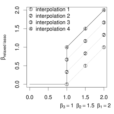
((a)) Solution paths of relaxed lasso

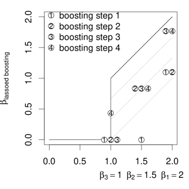
((b)) Solution paths of lassoed boosting

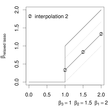
((c)) Step 2 in relaxed lasso

((d)) Step 2 in lassoed boosting

Figure 1: Figure 1(a) gives an example of the relaxed lasso solution paths for three parameters with linear interpolation weights $(0,0.33,0.66,1)$. Figure 1(b) is an example of boosting solution path for the same three parameters with four steps. Figures 1(c) and 1(d) select the coefficient solutions of the second interpolation and the second boosting step, respectively.

Remark 2.

Results in both simulation and application in this paper indicate that lassoed boosting sometimes may yield sparser models. Figures 1(c) and 1(d) give an illustration. Starting with an active set $\mathcal{A}_{q}=(\bm{\mathrm{x}}_{1},\bm{\mathrm{x}}_{2},\bm{\mathrm{x}}_{3})$, the relaxed lasso pulls the lasso solution, marked with \raisebox{-.9pt} {1}⃝, proportionately towards the LS solution, marked with \raisebox{-.9pt} {4}⃝ in Figure 1(a), and all three $\beta$’s increase in the second interpolation in Figure 1(c). With boosting, coefficients are updated one at a time and $\beta_{1}$ is not updated in step 2 in Figure 1(d) despite the fact that $\bm{\mathrm{x}}_{1}$ is already included in the active set. Hence, given the same set of variables in $\mathcal{A}_{q}$, LS-boost might spawn sparser solution paths than the relaxed lasso does.

Remark 3.

Solution paths of the relaxed lasso always include the LS solution for a given active set; this is not the case for LS-boost. After four steps, the relaxed lasso reaches the LS solution in Figure 1(a), while the final solution of LS-boost, marked with \raisebox{-.9pt} {4}⃝ in Figure 1(b), does not reach the same level. Early stopping based on an information criterion such as the corrected AIC in Hurvich et al. (1998) is a common practice in boosting to avoid overfitting. It is easy to verify that, for many data sets, a typical boosting solution stops in short of reaching the LS solution. One can increase the iteration number, but in practice there is no guarantee that the solution will be close to the LS solution even when $n>p$.

2.2 Convergence Results

In this section, we discuss the asymptotic convergence result of lassoed boosting. Let $\hat{\beta}^{\lambda_{q},k}$ be the boosting solution at step $k$ for the active set $\mathcal{A}_{q}$ associated with $\lambda_{q}$. Let $K_{\mathcal{A}_{q}}=|\mathcal{A}_{q}|$ be the cardinality of $\mathcal{A}_{q}$. The active set for the true model is $\mathcal{A}=\{1,\ldots,k\}$ and $K_{\mathcal{A}}=s$. We make the following assumptions for Propositions 1 and 2.

Assumption 1.

The data are generated according to eq. 1 with $u_{i}\sim(0,\sigma^{2})$. $\bm{\mathrm{X}}$ is deterministic.

Assumption 2.

The parameter vector is $s$-sparse so that $\beta^{*}=(\beta_{1},\ldots,\beta_{s},0,\ldots,0)^{T}$ and $s<p$.

No assumption on the relative growth between $n$ and $p$ is needed to prove our results. We do use the assumption $\log(p)/n\rightarrow 0$ to facilitate additional discussion in the Supplement (Section S.2).

2.2.1 Asymptotic rate

Proposition 1 shows that the asymptotic convergence rate of lassoed boosting.

Proposition 1.

Under Assumptions 1 and 2, as $n\rightarrow\infty$, we have

$$\inf_{\lambda_{q},k\in[1,\infty]}L_{n}(\hat{\beta}^{\lambda_{q},k})=O_{p}(n^{-1}).$$

The proof is given in Section S.1. Proposition 1 bears similarity to Theorem 6 in Meinshausen (2007). Compared to the slow convergence rate for the lasso in Theorem 5 in Meinshausen (2007), lassoed boosting has a faster convergence rate, a property shared with the relaxed lasso. Rigorously speaking, because we use Theorem 11.3 in Hastie et al. (2015) in the proof of Proposition 1, we need to borrow all assumptions in that theorem and the result in Proposition 1 holds with high probability.

The relaxed lasso and lassoed boosting share the same fast convergence rate because both of their solution paths include the LS solution when the lasso correctly recovers the variables. This observation suggests that any lasso-based two-stage method that includes the LS solution in the second step will also enjoy the rate in Proposition 1. We summarize the result in the next proposition. Let $\hat{\beta}_{\text{two-stage}}^{\lambda_{q},\mathcal{K}}$ be a two-stage estimator that uses either the lasso solution or the active set $\mathcal{A}_{q}$ to generates solution paths that include the full LS solution for each $\mathcal{A}_{q}$, and $\mathcal{K}$ is the vector of all tuning parameters in the second stage.

Proposition 2.

Under Assumptions 1 and 2, as $n\rightarrow\infty$,

$$\inf_{\lambda_{q},\mathcal{K}}L_{n}(\hat{\beta}_{\text{two-stage}}^{\lambda_{q},\mathcal{K}})=O_{p}(n^{-1}).$$

See Section Section S.1 for the proof. Proposition 2 indicates that the relaxed lasso and lassoed boosting are two examples of a class of two-stage estimators.

2.2.2 Linear convergence of predictions

Let $\hat{\beta}^{k}$ be the LS-boost solution at step $k$, $\hat{\beta}^{k}_{\text{LS}}$ be a possibly non-unique least squares solution at step $k$ on the active set $\mathcal{A}_{q}$, $\hat{\beta}_{\text{LS}}$ be the LS solution, and $\hat{\beta}_{\text{LS}}$ is non-unique when $p>n$. Theorem 2.1 in FGM gives the linear convergence result for $\lVert\bm{\mathrm{X}}\hat{\beta}^{k}-\bm{\mathrm{X}}\hat{\beta}_{\text{LS}}\rVert_{2}$. We investigate the convergence result for $\lVert\bm{\mathrm{X}}\hat{\beta}^{k}-\bm{\mathrm{X}}\beta^{*}\rVert_{2}$ in this section. Our discussion applies to LS-boost in general, but we will relate it to lassoed boosting.

Without any identification assumption, both $\hat{\beta}_{\text{LS}}$ and $\beta^{*}$ are underidentified. This is illustrated in Figure 2(a). In Figure 2(a), the boosting solution converges to $\hat{\beta}_{\text{LS}}$, which is one of many solutions in the “flat” sample solution region. The linear model in eq. 1 is also underidentified at the population level, leading to another “flat” population solution region in Figure 2(a). In general, the two regions are different in shape and position. Figures 2(b) and 2(c) give examples where the two regions may intersect each other and $L_{n}(\hat{\beta}_{LS})=L_{n}(\beta^{*})$ in Figure 2(c).

((a)) Separated solution regions

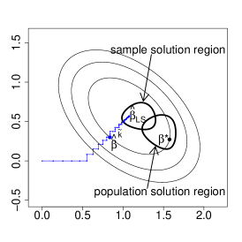
((b)) Overlapped solution regions

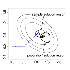
((c)) $\hat{\beta}_{LS}$ and $\beta^{*}$ have the same LS loss

Figure 2: The blue line is a LS-boost solution path starting from a zero vector and $\hat{\beta}^{\tilde{k}}$ is the boosting solution at step $\tilde{k}$. $L_{n}(\hat{\beta}_{LS})<L_{n}(\beta^{*})$ in Figures 2(a) and 2(b), and $L_{n}(\hat{\beta}_{LS})=L_{n}(\beta^{*})$ in Figure 1(c).

Let $\lambda_{\text{pmin}}(\bm{\mathrm{X}}^{T}\bm{\mathrm{X}})$ be the smallest nonzero eigenvalue of $\bm{\mathrm{X}}^{T}\bm{\mathrm{X}}$ and define

$$\gamma:=\left(1-\frac{\varepsilon(2-\varepsilon)\lambda_{\text{pmin}}(\bm{\mathrm{X}}^{T}\bm{\mathrm{X}})}{4p}\right).$$ (5)

FGM show that $0.75\leq\gamma<1$. Let $\nabla L_{n}(\beta)$ be the gradient vector at $\beta$.

Theorem 1.

Under Assumption 1, for $k\geq 0$, LS-boost has the following prediction bound

$$\lVert\bm{\mathrm{X}}\hat{\beta}^{k}-\bm{\mathrm{X}}\beta^{*}\rVert_{2}\leq\lVert\bm{\mathrm{X}}\hat{\beta}^{k}_{\text{LS}}\rVert_{2}\gamma^{k/2}+\sqrt{2n\lVert\nabla L_{n}(\beta^{*})\rVert_{2}\cdot\lVert\hat{\beta}_{\text{LS}}-\beta^{*}\rVert_{2}}.$$ (6)

A proof is given in the Online Supplement. Compared to Theorem 2.1 in FGM, eq. 6 has an extra term that relates to the gradient vector and the $\ell_{2}$ error of $\hat{\beta}_{\text{LS}}$. Without additional assumptions, this extra term will not disappear as $k\rightarrow\infty$.

Remark 4.

In the special case when $\beta^{*}$ is located inside the sample solution region (see Figure 2(c) for an example), $\lVert\nabla L_{n}(\beta^{*})\rVert_{2}=0$ and eq. 6 reduces to the result in Theorem 2.1 in FGM. This result holds even when $\lVert\hat{\beta}_{\text{LS}}-\beta^{*}\rVert_{2}>0$.

Clearly, eq. 6 indicates that, in a finite sample case when $n\not\to\infty$, LS-boost prediction will not recover the true sparse regression function, $\bm{\mathrm{X}}\beta^{*}$. Theorem 12.2 in Bühlmann and van de Geer (2011) (and Theorem 1 in Bühlmann (2006)) shows that, as both $n\to\infty$ and $k\to\infty$, $\lVert\bm{\mathrm{X}}\hat{\beta}^{k}-\bm{\mathrm{X}}^{T}\beta^{*}\rVert_{2}^{2}/n=o_{p}(1)$. This does not contradict the non-asymptotic result in eq. 6. We give a heuristic argument below.

Remark 5.

As $n\to\infty$ and sample data get closer to population, the sample solution region will converge, in both its shape and location, to the population solution region in Figure 2(a), and we expect $\nabla L_{n}(\beta^{*})\to 0$ in eq. 6 so that the second term in eq. 6 will disappear asymptotically and we will have $\lVert\bm{\mathrm{X}}\hat{\beta}^{k}-\bm{\mathrm{X}}\beta^{*}\rVert_{2}^{2}/n\rightarrow o_{p}(1)$ when $k\rightarrow\infty$. We provide a more detailed explanation in Section S.2.

Both Theorem 12.2 of Bühlmann and van de Geer (2011) and Theorem 1 present a prediction convergence result. How do they compare to each other? We give a brief remark below. See Section S.2 for a more detailed discussion.

Remark 6.

Theorem 1 uses an exponential function to the base of $\gamma$ to characterize the convergence of $\lVert\bm{\mathrm{X}}\hat{\beta}^{k}-\bm{\mathrm{X}}\beta^{*}\rVert_{2}^{2}/n$ as $k\rightarrow\infty$ while Theorem 12.2 in Bühlmann and van de Geer (2011) relies on a power function of $k$ to achieve the same goal.

Next, we discuss the faster convergence rate of lassoed boosting. Let $|\mathcal{A}_{q}|=p_{q}$. Consider two active sets $\mathcal{A}_{q_{1}}$ and $\mathcal{A}_{q_{2}}$. We will focus on the specific case when $p_{q_{1}}<p_{q_{2}}<n$ with either $n<p$ or $n\geq p$ and discuss why such case ($p_{q_{1}}<p_{q_{2}}<n$) is worth considering.

The linear convergence rate $\gamma$ plays a critical role in determining the speed of convergence in Theorem 1 and Theorem 2.1 in FGM. Figure 4 in FGM shows a general pattern that $\gamma$ decreases and $\lambda_{\text{pmin}}(\bm{\mathrm{X}}^{T}\bm{\mathrm{X}})$ increases as $p$ increases, though the these two relationships are not strictly monotonic. This seems to suggest that the convergence will be faster as $p$ increases, which can be seen from result (ii) in Theorem 2.1 of FGM

$$\lVert\hat{\beta}^{k}-\hat{\beta}_{\text{LS}}^{k}\rVert_{2}\leq\frac{\lVert\bm{\mathrm{X}}\hat{\beta}_{\text{LS}}\rVert_{2}}{\sqrt{\lambda_{\text{pmin}}(\bm{\mathrm{X}}^{T}\bm{\mathrm{X}})}}\gamma^{k/2}.$$ (7)

Similar conclusion can be drawn for the convergence result in Theorem 1. One, however, would expect the opposite: the convergence for the estimator, prediction, etc. will slow down when $p$ increases as more variables will add more “noise” and competition to the variable selection process.

We provide an alternative explanation to complement the results in Figure 4 in FGM. Notice that Figure 4 in FGM is drawn for cases when $p>n$ with $n=50$ and $p\geq 73$. The same figures will give a different pattern when $p<n$. In lassoed boosting, we sequentially apply LS-boost to variables in $\left\{\mathcal{A}_{q}\right\}_{q=1}^{Q}$. If the lasso does a good job in variable selection and one truly believes that the model is sparse, we expect some of the $\mathcal{A}_{q}$ in early stage of lasso variable selection will start to include the true variables and $|\mathcal{A}_{q}|\ll n$. For a sparse model, those active sets with $|\mathcal{A}_{q}|\ll n$ are arguably the most interesting ones since boosting solutions spawned on these sets will be more likely mimic the true, sparse elements in $\beta^{*}$. LS-boost on each $\mathcal{A}_{q}$ can be viewed as separate exercises and we can add the subscript $\mathcal{A}_{q}$ to results in Theorem 1 and eq. 7. Consider eq. 7 for the active set $\mathcal{A}_{q}$ with $|\mathcal{A}_{q}|\ll n$.

$$\lVert\hat{\beta}^{k}_{\mathcal{A}_{q}}-\hat{\beta}_{\text{LS},\mathcal{A}_{q}}^{k}\rVert_{2}\leq\frac{\lVert\bm{\mathrm{X}}_{\mathcal{A}_{q}}\hat{\beta}_{\text{LS},\mathcal{A}_{q}}\rVert_{2}}{\sqrt{\lambda_{\text{pmin}}(\bm{\mathrm{X}}_{\mathcal{A}_{q}}^{T}\bm{\mathrm{X}}_{\mathcal{A}_{q}})}}\gamma^{k/2}_{\mathcal{A}_{q}},$$ (8)

where all quantities are restricted to the active set $\mathcal{A}_{q}$ and

$$\gamma_{\mathcal{A}_{q}}:=\left(1-\frac{\varepsilon(2-\varepsilon)\lambda_{\text{pmin}}(\bm{\mathrm{X}}_{\mathcal{A}_{q}}^{T}\bm{\mathrm{X}}_{\mathcal{A}_{q}})}{4p_{q}}\right).$$ (9)

Since $|\mathcal{A}_{q}|<n$, all parameters can be identified. Next, we show a simulation result that describes $\gamma_{\mathcal{A}_{q}}$ and $\lambda_{\text{pmin}}(\bm{\mathrm{X}}_{\mathcal{A}_{q}}^{T}\bm{\mathrm{X}}_{\mathcal{A}_{q}})$ as a function of $|\mathcal{A}_{q}|$.

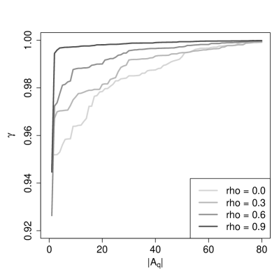
((a)) plot of $\gamma$ as $|\mathcal{A}_{q}|$ increases

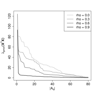
((b)) plot of $\lambda_{\text{pmin}}(\bm{\mathrm{X}}_{\mathcal{A}_{q}}^{T}\bm{\mathrm{X}}_{\mathcal{A}_{q}})$ as $|\mathcal{A}_{q}|$ increases

Figure 3: Simulation results for $\gamma_{\mathcal{A}_{q}}$ and $\lambda_{\text{pmin}}(\bm{\mathrm{X}}_{\mathcal{A}_{q}}^{T}\bm{\mathrm{X}}_{\mathcal{A}_{q}})$ with $n=100$ and $|\mathcal{A}_{q}|\leq 80$. The symbol “rho” refers to correlation among variables. Figure 3(a) shows $\gamma_{\mathcal{A}_{q}}$ is an increasing function of $|\mathcal{A}_{q}|$. Figure 3(b) shows $\lambda_{\text{pmin}}(\bm{\mathrm{X}}_{\mathcal{A}_{q}}^{T}\bm{\mathrm{X}}_{\mathcal{A}_{q}})$ is a decreasing function of $|\mathcal{A}_{q}|$.

Figure 3 describes the relationship of the linear convergence rate and minimum eigenvalue with $p_{q}(=|\mathcal{A}_{q}|)$ when $p_{q}<n$, and it reverses the pattens in Figure 4 in FGM. We stress that both figures are correct, but Figure 3 helps explain the convergence rate when $p_{q}<n$. As the lasso penalty parameter $\lambda_{q}$ decreases and $p_{q}$ increases, the minimum eigenvalue of $\bm{\mathrm{X}}_{\mathcal{A}_{q}}^{T}\bm{\mathrm{X}}_{\mathcal{A}_{q}}$ will decrease monotonically (and remain positive.) Such decrease in minimum eigenvalue as matrix dimension increases is a standard result in matrix theory, see, e.g., Theorem 4.3.8 in Horn and Johnson (1985). Figure 3(b) and eq. 9 imply Figure 3(a). Hence, for two active sets $\mathcal{A}_{q_{1}}$ and $\mathcal{A}_{q_{2}}$ with $p_{q_{1}}<p_{q_{2}}<n$, we have $\gamma_{\mathcal{A}_{q_{1}}}<\gamma_{\mathcal{A}_{q_{2}}}$ and the convergence rate for $\hat{\beta}^{k}_{\mathcal{A}_{q}}$ in eq. 8 is faster when boosting on $\mathcal{A}_{q_{1}}$ than on $\mathcal{A}_{q_{2}}$. This result applies to both eq. 8 and Theorem 1 after we replace $\bm{\mathrm{X}}^{T}\bm{\mathrm{X}}$ with $\bm{\mathrm{X}}_{\mathcal{A}_{q}}^{T}\bm{\mathrm{X}}_{\mathcal{A}_{q}}$ in lassoed boosting. This is beneficial particularly in early stages of the lasso, where $\mathcal{A}_{q}$ includes correct variables and $p_{q}<n$, the parameters are identified and the convergence rate is faster. Consequently, the convergence rate for prediction in Theorem 1 is also faster. When $|\mathcal{A}_{q}|>n$, parameters are underidentified and $\hat{\beta}_{\text{LS},\mathcal{A}_{q}}^{k}$ in eq. 8 may be different for each $k$ and $\mathcal{A}_{q}$.

3 Additional examples of two-stage procedure

In this section, we give several additional examples of two-stage estimators.

3.1 Lassoed forward stagewise regression

The forward stagewise regression algorithm in Hastie et al. (2009) is also a popular method to build coefficients and the regression function with small steps. In the $k$th step, it identifies the predictor $\bm{\mathrm{x}}_{j_{k}}$ most correlated with the current residual $\bm{\mathrm{r}}_{k}$ and makes the following update

$$\hat{\beta}_{j_{k}}^{k+1}=\hat{\beta}_{j_{k}}^{k}+\varepsilon\cdot\text{sign}(\bm{\mathrm{r}}_{k}^{T}\bm{\mathrm{x}}_{j_{k}}),\hat{\beta}_{j}^{k+1}=\hat{\beta}_{j}^{k}\text{ for }j\neq j_{k},\text{ and }\bm{\mathrm{r}}_{k+1}=\bm{\mathrm{r}}_{k}-\varepsilon\cdot\text{sign}(\bm{\mathrm{r}}_{k}^{T}\bm{\mathrm{x}}_{j_{k}})\bm{\mathrm{x}}_{j_{k}}.$$ (10)

This algorithm can also be implemented on lasso-generated active sets. We call it lassoed forward stagewise regression.

1 Assume a sequence of $Q$ tuning parameters $\left\{\lambda_{q}\right\}_{1}^{Q}$ for the lasso problem.

2 for $q=1$ to $Q$ do

3      Use lasso to obtain an active set of predictors, $\mathcal{A}_{q}$, for each $\lambda_{q}$.

4      Use forward stagewise regression to compute the coefficient path for each predictor in $\mathcal{A}_{q}$.

5      end for

return $Q$ sets of coefficient paths for validation (or cross-validation) purposes.

Algorithm 2 Lassoed forward stagewise regression

Mimicking Theorem 3.1 in FGM and Theorem 1, we give a prediction convergence result for Algorithm 2.

Theorem 2.

Let $k\geq 0$ be the number of iterations. Under Assumption 1, there exists an $i\in\left\{0,\cdots,k\right\}$ so that the following bound hold:

$$\lVert\bm{\mathrm{X}}\hat{\beta}^{i}-\bm{\mathrm{X}}\beta^{*}\rVert_{2}\leq\frac{\sqrt{p}}{\sqrt{\lambda}(\bm{\mathrm{X}}^{T}\bm{\mathrm{X}})}\left[\frac{\lVert\bm{\mathrm{X}}\hat{\beta}_{\text{LS}}\rVert_{2}^{2}}{\varepsilon(k+1)}+\epsilon\right]+\sqrt{2n\lVert\nabla L_{n}(\beta^{*})\rVert_{2}\cdot\lVert\hat{\beta}_{\text{LS}}-\beta^{*}\rVert_{2}}.$$ (11)

The proof is similar to that of Theorem 1 and is given in the Online Supplement. In the case of $p_{q}<n$, applying Theorem 2 to the active set $\mathcal{A}_{q}$ and using the same argument for lassoed boosting, we conclude that lassoed forward stagewise regression has a faster convergence rate compared to forward stagewise regression.

3.2 Twiced lasso

Hastie et al. (2009, p. 91) wrote, “one can use the lasso to select the set of non-zero predictors, and then apply the lasso again, but using only the selected predictors from the first step. This is known as the relaxed lasso (Meinshausen, 2007).” Here the idea of using lasso twice refers to the “Simple Algorithm” in Meinshausen (2007, p. 377), where we first obtain the active set $\mathcal{A}_{q}$ and then apply lasso again on $\mathcal{A}_{q}$ with $\lambda_{q+1},\cdots,\lambda_{Q}=0$. We provide a trivial extension of the relaxed lasso to facilitate its comparison with lassoed boosting and call it twiced lasso.

1 Assume a sequence of $Q$ tuning parameters $\left\{\lambda_{q}\right\}_{1}^{Q}$ for the lasso problem

2 for $q=1$ to $Q$ do

3      Use lasso to obtain an active set of variables, $\mathcal{A}_{q}$, for each $\lambda_{q}$.

4      Apply lasso again on $\mathcal{A}_{q}$ to compute the coefficient path for each predictor in $\mathcal{A}_{q}$ with $\left\{\lambda_{1},\cdots,\lambda_{Q}\right\}$.

5      end for

return $Q$ sets of coefficient paths for validation (or cross-validation) purposes

Algorithm 3 Twiced lasso

The key difference between twiced lasso in Algorithm 3 and the relaxed lasso is, in step 4 of Algorithm 3, twiced lasso always starts at $\lambda_{1}$ while the relaxed lasso starts at $\lambda_{q+1}$. Obviously, starting from $\lambda_{1}$ for every $\mathcal{A}_{q}$ creates redundancy in the computation. However, the formulation in Algorithm 3 allows us to make direct comparison with lassoed boosting in Algorithm 1 and helps explain the change in the convergence rate.

Adapt the restricted eigenvalues condition in equation (11.10) in Hastie et al. (2015) to the active set $\mathcal{A}_{q}$ and we have, for a constant $\tilde{\lambda}>0$,

$$\frac{\nu^{T}\left(\bm{\mathrm{X}}_{\mathcal{A}_{q}}^{T}\bm{\mathrm{X}}_{\mathcal{A}_{q}}/n\right)\nu}{\lVert\nu\rVert_{2}^{2}}\geq\tilde{\lambda}\text{ for all nonzero }\nu\text{ in a contrain set }\mathcal{C}.$$ (12)

The constrain set $\mathcal{C}$ defines directions along which parameters can be identified. The discussion on lassoed boosting also applies here. When the lasso does a good job in variable selection in step 3 of Algorithm 3, $\mathcal{A}_{q}$ contains the correct variables and $p_{q}<n$. In this case, the least-squares loss is strictly convex ($\nabla^{2}L_{n}(\beta)=\bm{\mathrm{X}}_{\mathcal{A}_{q}}^{T}\bm{\mathrm{X}}_{\mathcal{A}_{q}}/n\succ 0$) and eq. 12 holds for all $\nu\in\mathbb{R}^{p_{q}}$. Hence, $\tilde{\lambda}=\lambda_{\text{pmin}}(\bm{\mathrm{X}}_{\mathcal{A}_{q}}^{T}\bm{\mathrm{X}}_{\mathcal{A}_{q}}/n)$ and Figure 3(b) suggests $\tilde{\lambda}$ decreases as $p_{q}$ increases. Theorem 11.1 in Hastie et al. (2015) implies

$$\lVert\hat{\beta}_{\mathcal{A}_{q}}-\beta^{*}_{\mathcal{A}_{q}}\rVert_{2}\leq\frac{3}{\lambda_{\text{pmin}}(\bm{\mathrm{X}}_{\mathcal{A}_{q}}^{T}\bm{\mathrm{X}}_{\mathcal{A}_{q}}/n)}\sqrt{\frac{p_{q}}{n}}\sqrt{n}\lambda_{n},$$ (13)

where $\lambda_{n}$ is the tuning parameter such that $\lambda_{n}\geq 2\lVert\bm{\mathrm{X}}_{\mathcal{A}_{q}}^{T}\bm{\mathrm{u}}\rVert_{\infty}/n>0$. A smaller $p_{q}$ will make the bound in eq. 13 tighter, implying a faster convergence rate. We briefly summarize the discussion in the following remark.

Remark 7.

In twiced lasso, the first-stage screening can pare down the number of variables so that the second-stage lasso estimator can enjoy a faster convergence rate when $p_{q}<n$.

In eq. 13 when $p_{q}<s$, $\beta^{*}_{\mathcal{A}_{q}}$ is not necessarily equal to the corresponding elements in $\beta^{*}$ and its value varies, depending on $\bm{\mathrm{X}}_{\mathcal{A}_{q}}$. When $s\leq p_{q}<n$ and $\mathcal{A}_{q}$ correctly includes the nonzero variables, the non-zero elements of $\beta^{*}_{\mathcal{A}_{q}}$ are equal to those in $\beta^{*}$.

3.3 Twiced boosting

Another extension is to simply use boosting twice. Step 1 in Algorithm 4 uses LS-boost to screen variables and organizes them into sequentially increasing sets. Step 2 uses LS-boost again to grow the coefficient paths on each active set. The iteration stopping criterion in step 1 is when the active set includes all variables, while we can use the standard AIC-type criterion to stop boosting in the second stage.

1 Run a first round of LS-boost to obtain a sequence of $Q$ different active sets of variables, $\mathcal{A}_{q}$ with $q=1,\cdots,Q.$ \\not the same $\mathcal{A}_{q}$ from the lasso

2 for $q=1$ to $Q$ do

3      run LS-boost on each active set of variables, $\mathcal{A}_{q}$ and obtain coefficient paths for all predictors in $\mathcal{A}_{q}$.

4      end for

return $Q$ sets of coefficient paths for validation (or cross-validation) purposes

Algorithm 4 Twiced boosting

The algorithm in Algorithm 4 differs from the twin boosting algorithm in Bühlmann and Hothorn (2010). Twin boosting uses the estimate in the first stage to guide the selection of variable in the second stage, similar to the idea of adaptive lasso in Zou (2006).

4 Monte Carlo simulation

We conduct Monte Carlo simulations to study the performance of five estimators: forward stepwise, lasso, lassoed boosting, relaxed lasso, and twiced lasso. The best subset selection method in Bertsimas et al. (2016) is not considered here due to its computation cost. Our simulation design is the same as that in Hastie et al. (2020) except that, instead of 10, we use 50 equally spaced values between $0$ and $1$ as weights for the relaxed lasso.

4.1 Simulation setup

Let $\hat{\beta}$ be the estimated coefficient from one of the methods, beta-type be the pattern of sparsity, $\rho$ be the correlation among variables, and $v$ be the signal-to-noise (SNR) ratio. The simulation study has the following steps:

Step 1 data simulation

Choose a beta-type for $\beta^{*}$. Draw rows of $\bm{\mathrm{X}}$ i.i.d. from $N(0,\Sigma_{p\times p})$, where the $ij$th element of $\Sigma$ is $\rho^{|i-j|}$ with $\rho=0,0.35,0.7.$ Draw $\bm{\mathrm{y}}$ from $N(\bm{\mathrm{X}}\beta^{*},\sigma^{2}\bm{\mathrm{I}}_{n})$ and $\sigma^{2}={\beta^{*}}^{T}\Sigma\beta^{*}/v$.

Step 2 model selection

Run each of the five methods on $(\bm{\mathrm{X}},\bm{\mathrm{y}})$ with a sequence of tuning parameters; select a tuning parameter by minimizing prediction error on a validation set that is generated independent of and has the same size as $(\bm{\mathrm{X}},\bm{\mathrm{y}})$.

Step 3 model evluation

Record four metrics for model evaluation.

Step 4 average

Repeat steps 1 to 3 10 times and compute the averages of the metrics.

The SNR is $v=(0.05,0.09,0.14,0.25,0.71,1.22,2.07,3.52,6.00)$.

We consider four coefficient settings for the sparse coefficient $\beta^{*}$ in Step 1.

1. $\beta^{*}$ has $s$ elements equal to 1, placed at equally position between $1$ and $p$;

2. The first $s$ elements of $\beta^{*}$ equal to 1 and the rest equal to $0$;

3. The first $s$ elements of $\beta^{*}$ equal to $s$ interpolated values between $10$ and $0.5$ and the rest equal to $0$;

4. The first $s$ elements of $\beta^{*}$ equal to 1. The rest decays to $0$, $\beta^{*}_{i}=0.5^{i-s}$ for $i=s+1,\cdots,p$.

The first three beta-types are considered in Hastie et al. (2020), beta-type 5 is added in Hastie et al. (2020) and beta-type 4 in Bertsimas et al. (2016) is not considered due to its similar result to beta-type 3.

We consider the following four evaluation metrics at the test data $(\mathrm{x_{0},y_{0}})$:

• Relative risk

  $$\text{RR}(\hat{\beta})=\frac{E(x_{0}^{T}\hat{\beta}-x_{0}^{T}\beta^{*})^{2}}{E(x_{0}^{T}\beta^{*})^{2}}=\frac{(\hat{\beta}-\beta^{*})^{T}\Sigma(\hat{\beta}-\beta^{*})}{{\beta^{*}}^{T}\Sigma\beta^{*}}.$$

  $\text{RR}(\hat{\beta})=0$ if $\hat{\beta}=\beta^{*}$; $\text{RR}(\hat{\beta})=1$ if $\hat{\beta}=0$ (the null model.)

• Relative test error.

  $$\text{RTE}(\hat{\beta})=\frac{E(y_{0}-x_{0}^{T}\beta)^{2}}{\sigma^{2}}=\frac{(\hat{\beta}-\beta^{*})^{T}\Sigma(\hat{\beta}-\beta^{*})+\sigma^{2}}{\sigma^{2}}.$$

  $\text{RTE}(\hat{\beta})=1$ if $\hat{\beta}=\beta^{*}$; $\text{RTE}(\hat{\beta})=\text{SNR}+1$ if $\hat{\beta}=0$.

• Proportion of variance explained.

  $$\text{PVE}(\hat{\beta})=1-\frac{E(y_{0}-x_{0}^{T}\beta)^{2}}{\text{Var}(y_{0})}=1-\frac{(\hat{\beta}-\beta^{*})^{T}\Sigma(\hat{\beta}-\beta^{*})+\sigma^{2}}{{\beta^{*}}^{T}\Sigma\beta^{*}+\sigma^{2}}.$$

  $\text{PVE}(\hat{\beta})=\text{SNR}/(1+\text{SNR})$ if $\hat{\beta}=\beta^{*}$; $\text{RTE}(\hat{\beta})=0$ if $\hat{\beta}=0$.

• Number of nonzeros. $\text{NNZ}(\hat{\beta})=\lVert\hat{\beta}\rVert_{0}=\sum_{j=1}^{p}1\{\hat{\beta}_{j}\neq 0\}$. In figures that plot $\lVert\hat{\beta}\rVert_{0}$, we also print the number (averaged over 10 replications) of correctly identified coefficients for each method at each SNR level. This will allow us to infer the true and false positive rates in variable recovery.

We consider the following data size and sparsity combinations.

$$\begin{array}[]{ll}\bullet\text{ low: }n=100,p=10,s=5&\bullet\text{ medium: }n=500,p=100,s=5\\ \bullet\text{ high-5: }n=50,p=1000,s=5&\bullet\text{ high-10: }n=100,p=1000,s=10\end{array}$$

In total, we have $4(\text{beta-type})\times 4(\text{size and sparsity})\times 10(\text{SNR})\times 3(\rho)=480$ DGPs.

Parameter tuning again follows that in Hastie et al. (2020). We use the R package glmnet to generate the lasso solutions and to select variables for lassoed boosting. We use $50$ values of $\lambda$ in lasso in the low setting and $100$ values of $\lambda$ in the other three settings. We also use $50$ values of equally spaced weights between $0$ and $1$ for the relaxed lasso. The forward stepwise procedure is tuned up to $50$ steps. We use the R package $mboost$ to apply LS-boost to each active set of variables. Early stopping in boosting typically stops the estimates short of a LS solution, while the relaxed lasso can always reach a full LS solution. To reduce such difference between solutions of lassoed boosting and the relaxed lasso, we use the corrected AIC in Hurvich et al. (1998) to obtain the iteration number and double such number as the final stopping criterion in LS-boost. Note that even tripling or quadrupling the number will not guarantee a boosting solution to reach the LS solution. On the interval between $1$ and the final stopping criterion number, we select $50$ equally spaced steps and extract the corresponding LS-boost coefficients on each $\mathcal{A}_{q}$. The learning rate is set to be $0.01$.

Similar to Hastie et al. (2020), for all methods, we use a training set to generate solution pahts, a validation set to select the best solution, and a test set to compute the final prediction result. Hence there is no direct tuning of the lasso penalty parameter $\lambda$ in our results.

The computation time of lassoed boosting is more expensive than that of the relaxed lasso. If there are $100$ unique $\mathcal{A}_{q}$, by the time the lasso (and the relaxed lasso) finishes, lassoed boosting just gets started on the $100$ boosting jobs. Parallelization and warm starts are methods we can employ to improve the speed and reduce redundancy in the computation.

4.2 Simulation results

We discuss the simulation result by focusing on cases with beta-type 2 and $\rho=0.35$ based on validation tuning. The supplement includes the complete set of results for both validation and oracle tuning. We also skip the results of the twiced lasso, as they are similar to those of the relaxed lasso, and they are included in all figures in the Online Supplement.

Figures 4, 5, 6 and 7 plots the average of relative risk (RR), relative test error (RTE), proportion of variance explained (PVE), and number of nonzero (NNZ) coefficients for each of the data size and sparsity combinations over $10$ replications. The dotted line in RTE plots is the RTE of the null model; the dotted line in the PVE plots is the perfect score SNR/(1 + SNR); the horizontal dotted line in the number of nonzeros plots is the value of $s$. On top of each NNZ plot, we print the average (over 10 replications) number of correctly identified variables for each method at each of the 10 SNR levels, allowing us to easily infer the true positive rate.

In the RR plots across Figures 4, 5, 6 and 7, lassoed boosting and the relaxed lasso have very close performance, except for a small difference in Figure 6. In Figures 4 and 5 with small and medium settings, lassoed boosting and the relaxed lasso can outperform forward stepwise and the lasso when SNR is low; the performance of all four methods starts to converge when SNR increases. In Figures 6 and 7 with large $p$, forward stepwise and the lasso seem to outperform the other two methods when SNR is small. However, we needs to interpret some low SNR results with caution. For example, the NNZ plot shows the lasso, lassoed boosting, and the relaxed lasso can barely identify any correct variable, leading to an RR score larger than $1$; forward stepwise sticks to the null model at very low SNR values and obtains a null score of $RR=1$.

In all RTE plots in Figures 4, 5, 6 and 7, lassoed boosting and the relaxed lasso give almost the same performance, significantly outperforming the other two methods when SNR is relatively high. The only exception happens in Figure 5 where the RTE of forward stepwise becomes the smallest of the four when SNR is relatively large, though its numerical difference is small compared to that of lassoed boosting and the relaxed lasso.

In the PVE plots in Figures 4 and 5, all four methods give good results, which seems to further improve when SNR increases. This is not a surprise since an increased SNR helps all methods better identify the correct variables. In Figures 6 and 7, lassoed boosting and relaxed lasso perform similarly and show more advantage at most of the SNR levels.

In the NNZ plots across all four figures, lassoed boosting and the relaxed lasso show similar capability in sparsity recovery. In Figure 4, when SNR is relatively high, all methods recovers the true variables with the relaxed lasso outperforming lassoed boosting with slightly sparser models. But in the same figure when SNR decreases, we see lassoed boosting can sometimes give sparser models while identifying on average the same number of nonzero parameters. The NNZ plot in Figure 6 seems to suggest that relaxed lasso performs better in low SNR scenarios. This is not true in general. See the third row in Figure 8 for examples where lassoed boosting yields sparser models at low SNR levels. Again, notice that in Figure 6 almost no nonzero parameter is recovered when SNR is low, making any comparison less meaningful in this case.

Our analysis of the first three metrics seems to suggest that lassoed boosting and the relaxed lasso may share very similar coefficient paths. The NNZ plots in Figures 4, 5, 6 and 7 demonstrate that these two methods spawn different coefficient paths. To further corroborate this conclusion, we select several examples for beta-types 1 and 3 in Figure 8 from the Supplement, and it shows that lassoed boosting produces sparser models in quite a few cases. The figures also indicate that the lasso can recover the true parameters but its false inclusion rate is high.

Furthermore, with the information in the NNZ plots, we conclude that all methods fail to various extent at variable recovery when SNR is very low. This injects a note of caution in our interpretation of the other three metrics at low SNR levels.

Overall, with Figures 4, 5, 6 and 7 and many more in the Supplement, we can roughly conclude that lassoed boosting gives comparable performance to the relaxed lasso in the first three metrics and it can produce a sparser model under certain scenarios. We also need to be careful when drawing the conclusion of sparsity recovery. One can easily spot multiple occasions where the relaxed lasso gives sparser models.

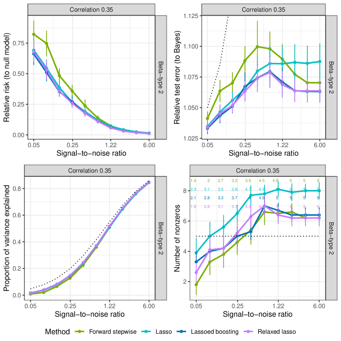
Figure 4: Curves of relative risk, relative test error, proportion of variance explained, and number of nonzeros as a function of SNR in the low setting with $n=100,p=10,$ and $s=5$. The numbers at the top of the number of nonzeros figure are the average correctly identified variables for each method at each of the $10$ SNR values. The order of the numbers, from row $1$ to row $4$, matches the order of four legend labels from left to right.

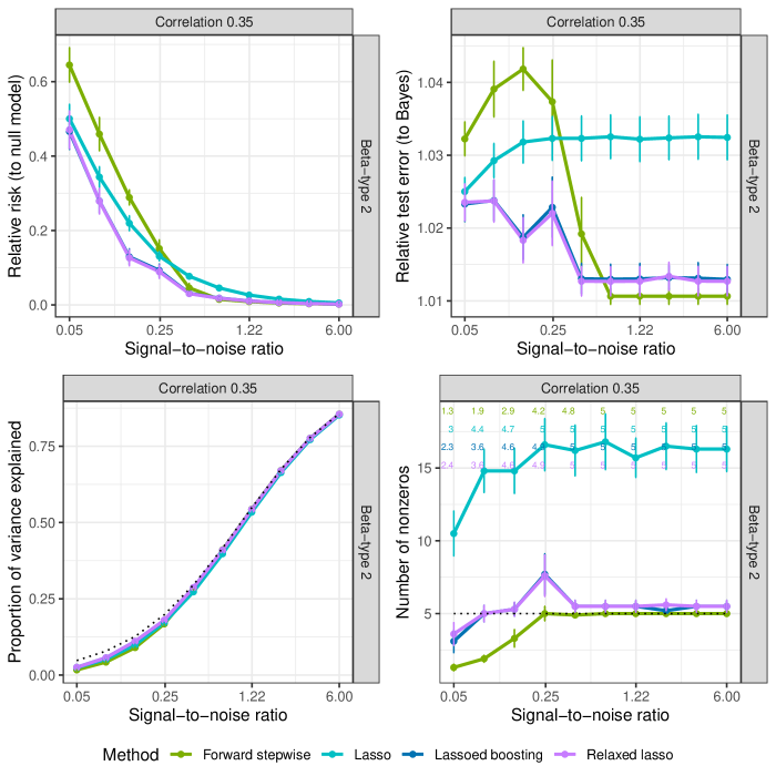
Figure 5: Curves of relative risk, relative test error, proportion of variance explained, and number of nonzeros as a function of SNR in the medium setting with $n=500,p=100,$ and $s=5$. The numbers at the top of the number of nonzeros figure are the average correctly identified variables for each method at each of the $10$ SNR values. The order of the numbers, from row $1$ to row $4$, matches the order of four legend labels from left to right.

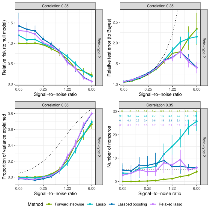
Figure 6: Curves of relative risk, relative test error, proportion of variance explained, and number of nonzeros as a function of SNR in the high-5 setting with $n=50,p=1000,$ and $s=5$. The numbers at the top of the number of nonzeros figure are the average correctly identified variables for each method at each of the $10$ SNR values. The order of the numbers, from row $1$ to row $4$, matches the order of four legend labels from left to right.

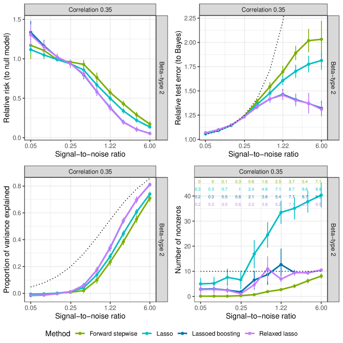
Figure 7: Curves of relative risk, relative test error, proportion of variance explained, and number of nonzeros as a function of SNR in the high-10 setting with $n=100,p=1000,$ and $s=10$. The numbers at the top of the number of nonzeros figure are the average correctly identified variables for each method at each of the $10$ SNR values. The order of the numbers, from row $1$ to row $4$, matches the order of four legend labels from left to right.

Figure 8: Top row: NNZ plots for beta-type 1 in the high-5 setting with $n=50,p=1000,s=5$. Middle row: NNZ plots for beta-type 1 in the high-10 setting with $n=100,p=1000,s=10$. Bottom row: NNZ plots for beta-type 3 in the low setting with $n=100,p=10,s=5$.The numbers at the top of each figure are the average correctly identified variables for each method at each of the $10$ SNR values. The order of the numbers, from row $1$ to row $4$, matches the order of four legend labels from left to right.

5 An application in equities return prediction

In this section we apply lassoed boosting to the application of predicting equity returns. We discuss the prediction accuracy of various methods and give an example of using path integrated gradient to compare the path differences between LS-boost and the lasso.

5.1 The prediction exercise

Green et al. (2017) use $94$ variables from the databases CRSP, Compustat and I/B/E/S to study the determinants of average monthly U.S. stock returns in a series of Fama-MacBeth regressions. We update their data to 2018 and use data from 2010 to 2018 in the application with a total of $376,544$ firm-month observations in $108$ months. The number of stocks (firms) in each month varies from $3,269$ to $3,883$. We add back $8$ variables that are removed in Green et al. (2017) due to collinearity concern. The dummy variable ipo is removed as it may have little variation during certain time period. In total, we have $101$($=94+8-1$) variables (see Section S.5 in Section S.5 for variable definitions.) Use January, 2010 as an example. There are $3,883$ observations in this month. $\bm{\mathrm{y}}$ in eq. 1 becomes a $3883\times 1$ vector of one-month-ahead, cross-section stock returns and $\bm{\mathrm{X}}$ includes all variables plus a column of ones for the intercept. Missing values are replaced by the mean of the variable. We use $50\%$, $25\%$, and $25\%$ of the $3,883$ observations for training, validation, and testing, respectively, and record the mean squared prediction error (MSPE) on the test set of that month. Repeat this exercise for the remaining $107$ months and we report the mean and median of the $108$ MSPEs.

We add a few comments before discussing the empirical results. The goal of our exercise is to find the a good linear model to predict stock returns (on a test set), which is different from identifying determinants to the cross-section of expected stock returns in the large finance literature on anomalies. The data we use ignore many macro variables and should not be considered as a complete collection of market information. Active arbitrage in the market also implies that all variables under consideration may have been carefully exploited by many analysts and we will not expect to see large predictive power of any linear model. The data also ignore some popular variables such as the Fama-French factors or the q-factors.

Table 1 reports the prediction results from different methods. The tuning procedure in simulation is also used for lasso, forward stepwise (FS), twiced lasso (TLasso), relaxed lasso (RLasso), and lassoed bossing ($\text{LB}_{1}$) in Table 1. $\text{LB}_{2}$ reports lassoed boosting with learning rate equal to $0.001$ and stopping criterion equal to the corrected AIC. GHZ represents a linear regression with $12$ variables identified in Green et al. (2017) that are significant in explaining the cross-section of stock returns. As pointed out in Green et al. (2017), these $12$ variables are only significant for the non-microcap return data before $2003$ and only two of them are significant for data after $2003$. We use the $12$-variable regression model for simple benchmarking purposes.

Table 1: Average MSPE and average model size of different methods

	Lasso	FS	TLasso	RLasso	$\text{LB}_{1}$	$\text{LB}_{2}$	GHZ
Mean	$0.020057$	$0.023027$	$0.020057$	$0.020046$	$0.020027$	$\mathbf{0.020015}$	$0.020455$
Median	$0.018206$	$0.021190$	$0.018212$	$0.018188$	$0.018221$	$\mathbf{0.018144}$	$0.018484$
# of tun. par.	$100$	$50$	$100\times 50$	$100\times 50$	$100\times 50$	$100\times 50$	N/A
avg. model size	$22.14$	$6.15$	$12.44$	$12.37$	$12.47$	$9.22$	$12$

• Notes: FS, TLasso, RLasso, and LB refer to forward stepwise, twiced lasso, relaxed lasso, and lassoed boosting respectively. GHZ in the last column refers to a linear regression model based on $12$ variables identified in Green et al. (2017) that are significant in explaining the cross-setion of expected returns for non-microcap stocks. Rows 1 and 2 report the mean and median of MSPE for the $108$ monthly test sets from January, 2010 to December, 2018. Row 3 reports the number of tuning parameters used, where the forward stepwise (FS) method is tuned over $50$ steps. Row 4 reports the average (over $108$ test sets) number of selected variables for each method. For the GHZ method, the number of variables (and model size) is fixed at $12$.

Razor-thin is perhaps the right adjective to describe the differences in prediction among the methods in Table 1. $\text{LB}_{1}$ does not seem to have any edge over the lasso or the relaxed lasso when using the same setting for tuning in the simulation section. The relaxed lasso outperforms the lasso with a smaller mean MSPE and a smaller median MSPE. The results of the twiced lasso closely follow those of the lasso and the relaxed lasso. When tuned with a learning rate of $0.001$, lassoed boosting starts to show some edge over all other methods. $\text{LB}_{2}$ has the smallest mean MSPE and median MSPE among all methods under consideration. We also observe the lasso and lasso-based methods all outperform the FS and the $12$-variable GHZ model.

The numerical difference between the relaxed lasso and lassoed boosting ($\text{LB}_{2}$) in Table 1 is very small. The difference in mean MSPE is $0.000031$. One may wonder does it even matter to have such a slim difference? We note that MSPE is defined as

$$\text{MSPE}=\frac{1}{n_{T}}\sum_{i=1}^{n_{T}}(y_{i}-x_{i}\hat{\beta})^{2},$$ (14)

where $n_{T}$ is the size of the test set. MSPE measures the average squared distance between prediction and the true value. By taking the square root of the MSPE, we obtain the average absolute distance, which is $0.0056$ ($=0.56\%$), and it translates to $56$ cents of difference when trading $100$ dollars. A practitioner can better assess the economic significance of this difference.

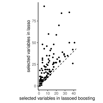
((a))

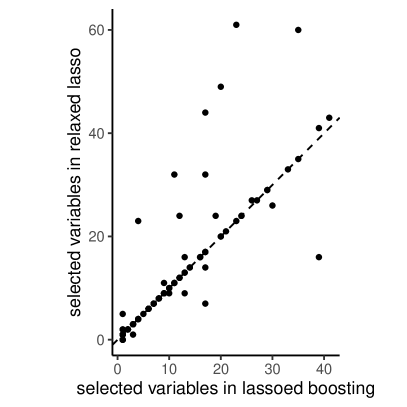
((b))

Figure 9: Each dot in the left figure represents the number of selected nonzeros in lassoed boosting and lasso for each of the $108$ test sets. The dotted line is the $45\text{\textdegree}$ line. Out of $108$ test sets, compared to lasso, lassoed boosting has smaller, bigger, and the equal model size in $(91,6,11)$ cases. The right figure is for the case of lassoed boosting vs. relaxed lasso, where the three numbers are $(25,14,69)$.

The last row of Table 1 reports the average number of selected variables across the $108$ test sets. On average, the number of selected variables in $\text{LB}_{2}$ is less than half of that in the lasso. Compared to the relaxed lasso, lassoed boosting can also offer a sparser solution on average. Figure 9 plots the number of nonzeros identified in lassoed boosting ($\text{LB}_{2}$) vs. those in the lasso (left figure) and the relaxed lasso (right figure) in the $108$ test sets. The dotted line is the $45\text{\textdegree}$ line. Out of $108$ test sets, lassoed boosting yields a sparser model in $91$ cases than the lasso does in the left figure. The competition for sparsity is more intense in the right figure: compared with the relaxed lasso, the number of nonzeros identified by lassoed boosting is smaller in $25$ cases, larger in $14$ cases, and the same in $69$ cases. Overall, our empirical results on model size is consistent with the findings in the simulation, that is, lassoed boosting can yield sparser model in certain cases. The large variation in model size also indicates model instability, though a stable model like GHZ underperforms those unstable models.

Combining the information in Table 1 and Figure 9, we conclude that, based on this application, lassoed boosting can deliver better prediction with a more compact model.

5.2 Path difference and parameter attribution

Common methods to compare the difference between the lasso and LS-boost include visual inspection of the solution paths, computing MSPEs, etc. We show that the integrated gradient along the solution paths of the lasso and LS-boost can also be used to study the difference between these two methods.

In many applications of network modeling, it is useful to attribute the prediction of a network to each inputs (variables). Sundararajan et al. (2017) propose the idea of integrated gradients for attribution. Consider a function $f:R^{p}\rightarrow R$. Given a $p\times 1$ input vector $z$, select a baseline vector $z^{\prime}$, the integrated gradient along the $j$th dimension on the straight line connecting $z$ and $z^{\prime}$ is defined as:

$$\text{integrated gradient}_{j}:=(z_{j}-z_{j}^{\prime})\times\int_{\alpha=0}^{1}\frac{\partial f(z^{\prime}+\alpha\times(z-z^{\prime}))}{\partial z_{j}}d\alpha,\text{ for }j=1,\cdots,p.$$ (15)

When the path connecting $z^{\prime}$ and $z$ is not a straight line, we can use the path integrated gradient for attribution.

$$\text{path integrated gradient}_{j}:=\int_{\alpha=0}^{1}\frac{\partial f(\phi(\alpha))}{\partial\phi_{j}(\alpha)}\frac{\partial\phi_{j}(\alpha)}{\partial\alpha}d\alpha,\text{ for }j=1,\cdots,p,$$ (16)

where $\phi=(\phi_{1},\cdots,\phi_{p}):[0,1]\rightarrow R^{p}$ is a function specifying a path linking $z^{\prime}$ and $z$ with $\phi(0)=z^{\prime}$ and $\phi(1)=z$.

Equations 15 and 16 describe a method for variable attribution. The same idea can be used for parameter attribution. To see that, consider the objective function in eq. 2 and let $f=L_{n}(\cdot)$. Since data are given, $f$ becomes a function of $\beta$. Let the $\hat{\beta}^{(0)}=\bm{\mathrm{0}}_{p\times 1}$ be the starting value in an algorithm (the $z$ in eq. 15) and $\hat{\beta}^{(1)}$ be the estimates at the end of the solution path (the $z^{\prime}$ in eq. 15). Since the solution path for the lasso and LS-boost is not a straight line connecting $\hat{\beta}^{(0)}$ and $\hat{\beta}^{(1)}$, we need to cumulate the gradients along the path on which the coefficients travel and use eq. 16. Without specifying a piecewise linear function $\phi$ for the lasso or LS-boost, we opt for the simple method of numerical integration based on the trapezoid rule. This method seems to work well in our case, probably due to the piecewise linear pattern of the solutions.

Use the data in January, 2010 as an example. Both the relaxed lasso and lassoed boost select the same $6$ variables (lev, mve, mom1m, baspread, mom12m, retvol) while the lasso selects $44$ variables. Assume both the lasso and LS-boost start with the same $6$ variables. Let the lasso use $1000$ equally spaced penalty values on $[0,\lambda_{0}]$ and LS-boost use the learning rate $0.1$ and iteration number $1000$ (the iteration number based on the corrected AIC is $127$.) Let $q$ denote the step in the lasso or LS-boost. We use the following formula for numerical integration. For $j=1,\cdots,6\text{ and }q=1,\cdots,1000$,

$$G_{jq}=\frac{\partial L_{n}(\hat{\beta}_{q+1})/\partial\beta_{j}+\partial L_{n}(\hat{\beta}_{q})/\partial\beta_{j}}{2}\times(\hat{\beta}_{q+1}-\hat{\beta}_{q}),$$ (17)

and we record eq. 17 as the $jq$th element of the matrix $G$. The approximation to the path integrated gradient in eq. 16 becomes the row sums of $G$

$$G_{j\cdot}=\sum_{q=1}^{1000}G_{jq},\text{ for }j=1,\cdots,6.$$ (18)

To gauge the precision of the numerical integration, we sum the starting value of the loss function $L_{n}(\hat{\beta}^{(0)})$ and $\sum_{j=1}^{6}G_{j\cdot}$, and compare it to the value of the loss function $L_{n}(\hat{\beta}^{(1)})$. For the lasso, the two quantities are equal up to the $8$th digit; for LS-boost, they are equal up to the $15$th digit. This simply verifies the fundamental theorem of calculus.

Table 2: Path integrated gradient for each $\beta$ in the lasso and LS-boost

	$\beta_{\text{lev}}$	$\beta_{\text{mve}}$	$\beta_{\text{mom1m}}$	$\beta_{\text{baspread}}$	$\beta_{\text{mom12m}}$	$\beta_{\text{retvol}}$
lasso	$-56.666$	$-32.765$	$-26.522$	$-9.864$	$-9.653$	$-3.661$
LS-boost	$-56.872$	$-32.803$	$-26.471$	$-9.777$	$-9.646$	$-3.561$

• Notes: See Section S.5 in the Supplement for the variable definition. The number in each cell is obtain via eq. 18. Multiply the numbers by $10^{-5}$ gives the actual path integrated gradients. The columns are arranged based on the order in which variables enter the model.

Table 2 reports the path integrated gradient for both the lasso and LS-boost. All numbers are negative because we consider function minimization. The variables are listed in the order in which they enter the lasso and LS-boost models. Because it is not possible for LS-boost to reach a full LS solution even with a large number of iterations, rigorously speaking, the numerical differences in these numbers also reflect a small numerical difference between the minimized loss of the lasso and LS-boost. In our case, the two minimized loss function based on demeaned data differ by less than $3\times 10^{-9}$. Hence, numerical difference in Table 2 is largely due to that fact the lasso and LS-boost visit difference solution paths. This provides a new perspective on understanding the difference between these two methods.

One should not conclude that the small numerical difference in Table 2 indicates the two methods always have similar parameter attribution. This is a simple regression model with only $6$ variables. With many variables, the two methods may select different models, and the attributions in Table 2 will be very different. This is likely to happen more frequently when comparing the lasso to lassoed boosting. Table 2 does not focus on the relaxed lasso. But it is interesting to note that the attribution method for the relaxed lasso is a hybrid procedure of using both eqs. 15 and 16.

((a)) SAPA in the lasso

((b)) SAPA in LS-boost, $\varepsilon=0.1$

Figure 10: SAPA in the lasso and LS-boost for $6$ variables (lev, mve, mom1m, baspread, mom12m, retvol) in January, 2010. In Figure 10(a), there is a small break at the end of the $5$th segment, resulting a total of $6$ segments.

We can also compute the column sums of $G$, which measures the stepwise aggregate parameter attribution (SAPA) of a method. SAPA is also the stepwise decrease in the loss function. Figure 10 plots SAPA of both the lasso and LS-boost. We make several observations. The SAPA of the lasso consists of $6$ segments, each of which represent a gradual decrease (in absolute value) in SAPA after a new variable enters the model. Interestingly, for LS-boost, its SAPA exhibits a more smooth, continuous pattern. This indicates that, the lasso and LS-boost may give completely different descending pattern of the loss function during optimization. For the lasso, SAPA at the beginning of each segment always shows up as a jump. This is due to the fact that when a new variable is just selected, its path integrated gradient at the current step is computed w.r.t. a zero value in its coefficient. After that, its path integrated gradient is computed w.r.t. a nonzero coefficient, which helps smooth the values, and they mostly line up along a straight path until the next variable enters the model. We also observe that these segments of the lasso SAPAs have different length and slope. A long and relatively flat segment indicates lasso is traveling on a solution path that might drive down the loss function considerably. The pattern of the SAPA in Figure 10(a) is also implicitly connected to the well-known fact that the lasso solution path is piecewise linear. Additional figures for cumulated parameter attribution in the Online Supplement can shed more light on these differences. Our analysis shows that path integrated gradient can be a useful tool to study the differences between the lasso and LS-boost. The above analysis also applies to lassoed boosting.

6 Conclusions

This paper proposes lassoed boosting as a refitting strategy based on the lasso, and it is found to have good finite sample property in both our simulation experiment and an application. We also introduce the idea of using path integrated gradient to study the difference between the lasso and LS-boost in parameter attribution.

We compare only five variable selection methods and use just one dataset in our application. It takes one line of R code to connect our method to the bestsubset package in Hastie et al. (2020) and reproduce the simulation results (see the github page for instructions.) We invite readers to try lassoed boosting in more simulations and applications to further study its property.

Our work can be extended in several directions. First, it will be interesting to compare lassoed boosting to other methods in a classification exercise such as credit rating and default analysis. Second, it will be useful to attach a valid p-value to estimates from lassoed boosting. Third, Proposition 2 suggests that both the relaxed lasso and lassoed boosting are examples of possibly many other two-stage approaches, and an analyst can explore other possibilities to find a better method. We leave these topics for future research.

SUPPLEMENTARY MATERIAL TO “LASSOED BOOSTING AND LINEAR PREDICTION IN EQUITIES MARKET”

Xiao Huang

This supplement contains all proofs, additional discussions and figures.

S.1 Proofs

Proof of Proposition 1.

From Theorem 11.3 in Hastie et al. (2015), we know there exists a $\lambda$ such that lasso is variable selection consistent as $n\rightarrow\infty$. Let $\lambda_{*}$ be such a penalty value so that $\mathcal{A}_{\lambda_{*}}=\mathcal{A}$. Given the correctly identified active set $\mathcal{A}_{\lambda_{*}}$, the LS-boost solution at step $k=\infty$ is equal to the LS solution on the active set $\mathcal{A}_{\lambda_{*}}$, $\hat{\beta}^{\lambda_{*},\infty}=\hat{\beta}_{LS}^{\lambda_{*}}$. Since $\inf_{\lambda,s\in[1,\infty]}L_{n}(\hat{\beta}^{\lambda,k})\leq L_{n}(\hat{\beta}_{LS}^{\lambda_{*}})$, we have, for $c>0$,

$$P(\inf_{\lambda,k\in[1,\infty]}L_{n}(\hat{\beta}^{\lambda,k})>cn^{-1}) \leq P(L_{n}(\hat{\beta}^{\lambda_{*}}_{LS})>cn^{-1})\rightarrow 0\text{ as }n\rightarrow\infty,$$

where the last result follows standard convergence property of a LS estimator. ∎

Proof of Proposition 2.

The proof is similar to the proof of Proposition 1. Using Theorem 11.3 in Hastie et al. (2015), as $n\rightarrow\infty$, gives a $\lambda_{*}$ so that $\mathcal{A}_{\lambda_{*}}=\mathcal{A}$ with high probability. Since $\inf_{\lambda,\mathcal{K}}L_{n}(\hat{\beta}^{\lambda,\mathcal{K}})\leq L_{n}(\hat{\beta}_{LS}^{\lambda_{*}})$ as the tuning vector $\mathcal{K}$ can generate the case of a full LS solution, we have, for $c>0$,

$$P(\inf_{\lambda,\mathcal{K}}L_{n}(\hat{\beta}^{\lambda,\mathcal{K}})>cn^{-1}) \leq P(L_{n}(\hat{\beta}^{\lambda_{*}}_{LS})>cn^{-1})\rightarrow 0\text{ as }n\rightarrow\infty,$$

where the last result again follows standard convergence property of a LS estimator. ∎

Proof of Theorem 1.

By triangular inequality, we have

$$\lVert\bm{\mathrm{X}}\hat{\beta}^{k}-\bm{\mathrm{X}}\beta^{*}\rVert_{2}\leq\lVert\bm{\mathrm{X}}\hat{\beta}^{k}-\bm{\mathrm{X}}\hat{\beta}_{\text{LS}}\rVert_{2}+\lVert\bm{\mathrm{X}}\hat{\beta}_{\text{LS}}-\bm{\mathrm{X}}\beta^{*}\rVert_{2},$$ (S.1)

where the bound for the term $\lVert\bm{\mathrm{X}}\hat{\beta}^{k}-\bm{\mathrm{X}}\hat{\beta}_{\text{LS}}\rVert_{2}$ is given in Theorem 2.1 in Freund et al. (2017). Consider the second term $\lVert\bm{\mathrm{X}}\hat{\beta}_{\text{LS}}-\bm{\mathrm{X}}\beta^{*}\rVert_{2}$. Recall $L_{n}(\beta^{*})\geq L_{n}(\hat{\beta}_{\text{LS}})$.

$$2n(L_{n}(\beta^{*})-L_{n}(\hat{\beta}_{\text{LS}})) =\lVert\bm{\mathrm{y}}-\bm{\mathrm{X}}\beta^{*}\rVert^{2}_{2}-\lVert\bm{\mathrm{y}}-\bm{\mathrm{X}}\hat{\beta}_{\text{LS}}\rVert^{2}_{2}$$

$$=-2\bm{\mathrm{y}}^{T}\bm{\mathrm{X}}\beta^{*}+\lVert\bm{\mathrm{X}}\beta^{*}\rVert^{2}_{2}+2\bm{\mathrm{y}}^{T}\bm{\mathrm{X}}\hat{\beta}_{\text{LS}}-\lVert\bm{\mathrm{X}}\hat{\beta}_{\text{LS}}\rVert^{2}_{2}$$

$$=-2\hat{\beta}_{\text{LS}}\bm{\mathrm{X}}^{T}\bm{\mathrm{X}}\beta^{*}+\lVert\bm{\mathrm{X}}\beta^{*}\rVert^{2}_{2}+2\hat{\beta}_{\text{LS}}\bm{\mathrm{X}}^{T}\bm{\mathrm{X}}\hat{\beta}_{\text{LS}}-\lVert\bm{\mathrm{X}}\hat{\beta}_{\text{LS}}\rVert^{2}_{2}$$

$$=\lVert\bm{\mathrm{X}}\hat{\beta}_{\text{LS}}-\bm{\mathrm{X}}\beta^{*}\rVert^{2}_{2},$$

where we use the f.o.c. of eq. 2, $\bm{\mathrm{y}}^{T}\bm{\mathrm{X}}=\hat{\beta}_{\text{LS}}\bm{\mathrm{X}}^{T}\bm{\mathrm{X}}$, in the third equality. Hence, we have

$$\lVert\bm{\mathrm{X}}\hat{\beta}_{\text{LS}}-\bm{\mathrm{X}}\beta^{*}\rVert_{2}=\sqrt{2n(L_{n}(\beta^{*})-L_{n}(\hat{\beta}_{\text{LS}}))}$$ (S.2)

By the convexity of $L_{n}(\cdot)$, we have

$$L_{n}(\hat{\beta}_{\text{LS}}) \geq L_{n}(\beta^{*})+\nabla L_{n}(\beta^{*})^{T}(\hat{\beta}_{\text{LS}}-\beta^{*})$$

$$\geq L_{n}(\beta^{*})-\lVert\nabla L_{n}(\beta^{*})\rVert_{2}\cdot\lVert\hat{\beta}_{\text{LS}}-\beta^{*}\rVert_{2}.$$

Rearranging the last inequality gives

$$L_{n}(\beta^{*})-L_{n}(\hat{\beta}_{\text{LS}})\leq\lVert\nabla L_{n}(\beta^{*})\rVert_{2}\cdot\lVert\hat{\beta}_{\text{LS}}-\beta^{*}\rVert_{2}.$$ (S.3)

Substituting Theorem 2.1 (iii) in FGM and eqs. S.2 and S.3 into eq. S.1 completes the proof. ∎

Proof of Theorem 2.

Applying the triangular inequality, we have

$$\lVert\bm{\mathrm{X}}\hat{\beta}^{i}-\bm{\mathrm{X}}\beta^{*}\rVert_{2}\leq\lVert\bm{\mathrm{X}}\hat{\beta}^{i}-\bm{\mathrm{X}}\hat{\beta}_{\text{LS}}\rVert_{2}+\lVert\bm{\mathrm{X}}\hat{\beta}_{\text{LS}}-\bm{\mathrm{X}}\beta^{*}\rVert_{2}.$$ (S.4)

Bound for the first term on the r.h.s. follows Theorem 3.1 (iii) in FGM, while bound for the second term on the r.h.s. follows the same result in the proof of Theorem 1. Combining the two results gives the bound in Theorem 2. ∎

S.2 Comparison of convergence results in Theorem 1 and Theorem 12.2 in Bühlmann and van de Geer (2011)

The convergence rate in Theorem 12.2 in Bühlmann and van de Geer (2011) is obtained after choosing an iteration number $k$ (“$m$” in the book’s notation) to minimize the upper bound. We can consider the pre-optimized rate result in the first equation on page 426 of Bühlmann and van de Geer (2011) to more easily gain some insight. For ease of reference, we reproduce the equation below.

$$\frac{1}{n}\lVert\bm{\mathrm{X}}\hat{\beta}^{k}-\bm{\mathrm{X}}\beta^{*}\rVert_{2}^{2}=\lVert\hat{R}^{k}f^{0}\rVert_{n}^{2}\leq\max\{2k^{-\frac{D_{\kappa}}{2+D_{\kappa}}},\kappa^{-1}(1-\kappa/2)^{-1}2\Delta_{n}(\lVert\beta^{0}_{n}\rVert_{1}+k\gamma_{n})+k\Delta_{n}\},$$ (S.5)

where we replace “$m$” in the original equation with $k$ to indicate the boosting iteration number, and

$$f^{0} =\bm{\mathrm{X}}\beta^{0}_{n}\text{ (and }\beta^{0}_{n}=\beta^{*}\text{ in this paper),}$$

$$\hat{R}^{k}f^{0} =\bm{\mathrm{X}}\beta_{n}^{0}-\bm{\mathrm{X}}\hat{\beta}^{k},$$

$$\kappa \in(0,\frac{1}{2}),$$

$$D_{\kappa} =(1-\kappa)(1-\kappa/2),$$

$$\Delta_{n} =\max_{j=1,\cdots,p}\frac{1}{n}\sum_{i=1}^{n}|u_{i}x_{ij}|=O_{p}(\sqrt{\log(p)/n}),$$

$$\gamma_{n} =(1+\sigma^{2})+o_{p}(1)=O_{p}(1).$$

Under the assumption of $\lVert\beta^{0}_{n}\rVert_{1}=o\left(\sqrt{\frac{n}{\log(p)}}\right)$ and $k=o(\sqrt{n/\log(p)})$ in the same theorem, the second term in eq. S.5 is dominated by $\kappa^{-1}(1-\kappa/2)^{-1}2\Delta_{n}\lVert\beta^{0}_{n}\rVert_{1}$, which has order $\Delta_{n}\lVert\beta^{0}_{n}\rVert_{1}$. Although it is $o_{p}(1)$, it is not a function of $k$ and we cannot compare it directly to the result in Theorem 1. For this reason, let us consider the first term in eq. S.5.

Given the value of $\kappa$, $\frac{D_{\kappa}}{2+D_{\kappa}}$ varies on the interval $(0.158,0.333)$. Hence $2k^{-\frac{D_{\kappa}}{2+D_{\kappa}}}$ is a power function of $k$ with its power in the interval of $(-0.333,-0.158)$.

From Theorems 1 and S.1, we have

$$\frac{1}{n}\lVert\bm{\mathrm{X}}\hat{\beta}^{k}-\bm{\mathrm{X}}\beta^{*}\rVert_{2}^{2} \leq\frac{1}{n}\lVert\bm{\mathrm{X}}\hat{\beta}^{k}_{\text{LS}}\rVert_{2}^{2}\gamma^{k}+\frac{1}{n}\lVert\bm{\mathrm{X}}\hat{\beta}_{\text{LS}}-\bm{\mathrm{X}}\beta^{*}\rVert_{2}$$

$$\leq\frac{1}{n}\lVert\bm{\mathrm{y}}\rVert_{2}^{2}\gamma^{k}+\frac{1}{n}\lVert\bm{\mathrm{X}}\hat{\beta}_{\text{LS}}-\bm{\mathrm{X}}\beta^{*}\rVert_{2},$$ (S.6)

where we can assume $\frac{2}{n}\lVert\bm{\mathrm{y}}\rVert_{2}^{2}=O_{p}(1)$. Hence the first term on the r.h.s. of eq. S.6 is an exponential function to the base of $\gamma$ with $\gamma\in[0.75,1)$. Thus, we conclude that while Theorem 2.12. in Bühlmann and van de Geer (2011) uses a power function to describe the convergence of prediction in LS-boost as the procedure iterates, Theorem 1 (and Theorem 2.1 in FGM) uses an exponential function to characterize the convergence.

With additional assumptions, we can further comment on the behavior of the second term on the r.h.s. of eq. S.6. Assume the error term $u_{i}$ belongs to the class of sub-Gaussian distribution with variance proxy $\sigma^{2}$, $u_{i}\sim\text{subG}(\sigma^{2})$. If $p\leq n$, Theorem 2.2 in Rigollet and Hütter (2019) shows the second term is $O_{p}(1/n)$; if $p>n$ and $\beta^{*}$ is $s$-sparse, Corollary 2.8 in Rigollet and Hütter (2019) indicates that the second term is $O_{p}(\log(p)/n)$. These results hold with high probability. To summarize, under the additional assumption of $O_{p}(\log(p)/n)\rightarrow 0$ as $n,p\rightarrow\infty$, the second term in eq. S.6 disappears asymptotically, which allows us to focus on the exponential function, $\gamma^{k}$, to study the convergence of predictions in LS-boost.

S.3 Validation tuning figures in simulation

S.3.1 Low setting: $n=100,p=10,s=5$

S.3.1.1 Relative risk (to null model)

S.3.1.2 Relative test error (to Bayes)

S.3.1.3 Proportion of variance explained

S.3.1.4 Number of nonzero coefficients

S.3.2 Medium setting: $n=500,p=100,s=5$

S.3.2.1 Relative risk (to null model)

S.3.2.2 Relative test error (to Bayes)

S.3.2.3 Proportion of variance explained

S.3.2.4 Number of nonzero coefficients

S.3.3 High-5 setting: $n=50,p=1000,s=5$

S.3.3.1 Relative risk (to null model)

S.3.3.2 Relative test error (to Bayes)

S.3.3.3 Proportion of variance explained

S.3.3.4 Number of nonzero coefficients

S.3.4 High-10 setting: $n=100,p=1000,s=10$

S.3.4.1 Relative risk (to null model)

S.3.4.2 Relative test error (to Bayes)

S.3.4.3 Proportion of variance explained

S.3.4.4 Number of nonzero coefficients

S.4 Oracle tuning figures in simulation

S.4.1 Low setting: $n=100,p=10,s=5$

S.4.1.1 Relative risk (to null model)

S.4.1.2 Relative test error (to Bayes)

S.4.1.3 Proportion of variance explained

S.4.1.4 Number of nonzero coefficients

S.4.2 Medium setting: $n=500,p=100,s=5$

S.4.2.1 Relative risk (to null model)

S.4.2.2 Relative test error (to Bayes)

S.4.2.3 Proportion of variance explained

S.4.2.4 Number of nonzero coefficients

S.4.3 High-5 setting: $n=50,p=1000,s=5$

S.4.3.1 Relative risk (to null model)

S.4.3.2 Relative test error (to Bayes)

S.4.3.3 Proportion of variance explained

S.4.3.4 Number of nonzero coefficients

S.4.4 High-10 setting: $n=100,p=1000,s=10$

S.4.4.1 Relative risk (to null model)

S.4.4.2 Relative test error (to Bayes)

S.4.4.3 Proportion of variance explained

S.4.4.4 Number of nonzero coefficients

S.5 Variable definitions in application

Variables used in the application (Table 1 in Green et al. (2017))
( continued )   Acronym	Firm characteristic	Acronym	Firm characteristic
absacc	Absolute accruals	divo	Dividend omission
acc	Working capital accruals	dolvol	Dollar trading volume
aeavol	Abnormal earnings	dy	Dividend to price
	announcement volume
age	# years since first	ear	Earnings announcement
	Compustat coverage		return
agr	Asset growth	egr	Growth in common
			shareholder equity
baspread	Bid-ask spread	ep	Earnings to price
beta	Beta	fgr5yr	Forecasted growth in
			5-year EPS
betasq	Beta squared	gma	Gross proftability
bm	Book-to-market	grCAPX	Growth in capital
			expenditures
bm_ia	Industry-adjusted book to	grltnoa	Growth in long-term net
	market		operating assets
cash	Cash holdings	herf	Industry sales
			concentration
cashdebt	Cash flow to debt	hire	Employee growth rate
cashpr	Cash productivity	idiovol	Idiosyncratic return
			volatility
cfp	Cash-flow-to-price ratio	ill	Illiquidity
cfp_ia	Industry-adjusted	indmom	Industry momentum
	cash-flow-to-price ratio
chatoia	Industry-adjusted change	invest	Capital expenditures and
	in asset turnover		inventory
chcsho	Change in shares	IPO	New equity issue
	outstanding
chempia	Industry-adjusted change	lev	Leverage
	in employees
chfeps	Change in forecasted EPS	lgr	Growth in long-term debt
chinv	Change in inventory	maxret	Maximum daily return
chmom	Change in 6-month	mom12m	12-month momentum
	momentum
chnanalyst	Change in number of	mom1m	1-month momentum
	analysts
chpmia	Industry-adjusted change in profit margin	mom36m	36-month momentum
chtx	Change in tax expense	mom6m	6-month momentum
cinvest	Corporate investment	ms	Financial statement score
convind	Convertible debt indicator	mve	Size
currat	Current ratio	mve_ia	Industry-adjusted size
depr	Depreciation / PP&E	nanalyst	Number of analysts
			covering stock
disp	Dispersion in forecasted	nincr	Number of earnings
	EPS		increases
divi	Dividend initiation	operprof	Operating proftability
orgcap	Organizational capital	roeq	Return on equity
pchcapx_ia	Industry adjusted %	roic	Return on invested capital
	change in capital expenditures
pchcurrat	% change in current ratio	rsup	Revenue surprise
pchdepr	% change in depreciation	salecash	Sales to cash
pchgm_pchsale	% change in gross margin	saleinv	Sales to inventory
	- % change in sales
pchquick	% change in quick ratio	salerec	Sales to receivables
pchsale_pchinvt	% change in sales	secured	Secured debt
	- % change in inventory
pchsale_pchrect	% change in sales	securedind	Secured debt indicator
	- % change in A/R
pchsale_pchxsga	% change in sales	sfe	Scaled earnings forecast
	- % change in SG&A
pchsaleinv	% change	sgr	Sales growth
	sales-to-inventory
pctacc	Percent accruals	sin	Sin stocks
pricedelay	Price delay	SP	Sales to price
ps	Financial statements score	std_dolvol	Volatility of liquidity
			(dollar trading volume)
quick	Quick ratio	std_turn	Volatility of liquidity
			(share turnover)
rd	R&D increase	stdacc	Accrual volatility
rd_mve	R&D to market	stdcf	Cash flow volatility
	capitalization
rd_sale	R&D to sales	sue	Unexpected quarterly
			earnings
realestate	Real estate holdings	tang	Debt capacity/firm
			tangibility
retvol	Return volatility	tb	Tax income to book
			income
roaq	Return on assets	turn	Share turnover
roavol	Earnings volatility	zerotrade	Zero trading days

S.6 Additional figures for parameter attribution in the lasso and LS-boost

Figures 11(a), LABEL:fig:areaboost01 and 11(d) plot, at each step, a parameter estimate $\hat{\beta}_{j}$’s stepwise cumulative parameter attribution (SCPA) as a percentage of the cumulative aggregate parameter attribution (CAPA) up to each step. These three figures provide an additional way to visualize the difference between the lasso and LS-boost. Compared with Figure 10(b), Figure 11(c) illustrates how a different learning rate can alter the pattern of SAPA in LS-boost.

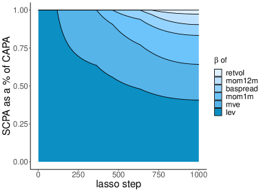
((a)) SCPA plot for the lasso

((c)) SAPA in LS-boost, $\varepsilon=0.01$

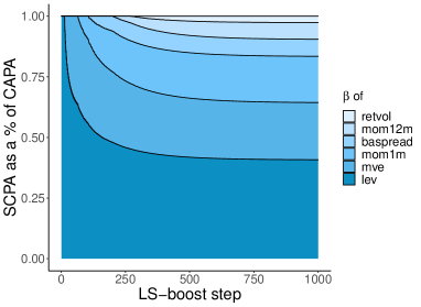
((d)) SCPA plot for LS-boost, $\varepsilon=0.01$

Figure 11: Figures 11(a), LABEL:fig:areaboost01 and 11(d) are SCPA plots for lasso and LS-boost. Figure 11(c) is the SAPA plot for LS-boost with $\varepsilon=0.01$.

References

- Bertsimas et al. (2016) Bertsimas, D., King, A. and Mazumder, R. (2016). Best subset selection via a modern optimization lens. The Annals of Statistics, 44 (2), 813 – 852.
- Bühlmann (2006) Bühlmann, P. (2006). Boosting for high-dimensional linear models. The Annals of Statistics, 34 (2), 559 – 583.
- Bühlmann and Hothorn (2010) Bühlmann, P. and Hothorn, T. (2010). Twin boosting: improved feature selection and prediction. Statistics and Computing, 20 (2), 119 – 138.
- Bühlmann and van de Geer (2011) — and van de Geer, S. (2011). Statistics for High-Dimensional Data. Springer series in statistics, Springer, 1st edn.
- Chzhen et al. (2019) Chzhen, E., Hebiri, M. and Salmon, J. (2019). On Lasso refitting strategies. Bernoulli, 25 (4A), 3175 – 3200.
- Fan and Li (2001) Fan, J. and Li, R. (2001). Variable selection via nonconcave penalized likelihood and its oracle properties. Journal of the American Statistical Association, 96 (456), 1348–1360.
- Freund et al. (2017) Freund, R. M., Grigas, P. and Mazumder, R. (2017). A new perspective on boosting in linear regression via subgradient optimization and relatives. The Annals of Statistics, 45 (6), 2328–2364.
- Friedman (2001) Friedman, J. H. (2001). Greedy function approximation: A gradient boosting machine. The Annals of Statistics, 29 (5), 1189–1232.
- Green et al. (2017) Green, J., Hand, J. R. M. and Zhang, X. F. (2017). The Characteristics that Provide Independent Information about Average U.S. Monthly Stock Returns. The Review of Financial Studies, 30 (12), 4389–4436.
- Hastie et al. (2009) Hastie, T., Tibshirani, R. and Friedman, J. (2009). The Elements of Statistical Learning: Data Mining, Inference, and Prediction. Springer series in statistics, Springer, 2nd edn.
- Hastie et al. (2020) —, — and Tibshirani, R. (2020). Best Subset, Forward Stepwise or Lasso? Analysis and Recommendations Based on Extensive Comparisons. Statistical Science, 35 (4), 579 – 592.
- Hastie et al. (2015) —, — and Wainwright, M. (2015). Statistical Learning with Sparcity: The Lasso and Generalizations. Chapman and Hall/CRC.
- Horn and Johnson (1985) Horn, R. A. and Johnson, C. R. (1985). Matrix Analysis. Cambridge University Press.
- Hurvich et al. (1998) Hurvich, C. M., Simonoff, J. S. and Tsai, C.-L. (1998). Smoothing parameter selection in nonparametric regression using an improved akaike information criterion. Journal of the Royal Statistical Society: Series B (Statistical Methodology), 60 (2), 271–293.
- Mazumder et al. (2011) Mazumder, R., Friedman, J. H. and Hastie, T. (2011). Sparsenet: Coordinate descent with nonconvex penalties. Journal of the American Statistical Association, 106 (495), 1125–1138, pMID: 25580042.
- Meinshausen (2007) Meinshausen, N. (2007). Relaxed lasso. Computational Statistics & Data Analysis, 52 (1), 374–393.
- Sundararajan et al. (2017) Sundararajan, M., Taly, A. and Yan, Q. (2017). Axiomatic attribution for deep networks. In Proceedings of the 34th International Conference on Machine Learning - Volume 70, ICML’17, JMLR.org, p. 3319–3328.
- Tibshirani (1996) Tibshirani, R. (1996). Regression shrinkage and selection via the lasso. Journal of the Royal Statistical Society. Series B (Statistical Methodology), 58 (1), 267–288.
- Yuan and Lin (2006) Yuan, M. and Lin, Y. (2006). Model selection and estimation in regression with grouped variables. Journal of the Royal Statistical Society: Series B (Statistical Methodology), 68 (1), 49–67.
- Zhang (2010) Zhang, C.-H. (2010). Nearly unbiased variable selection under minimax concave penalty. The Annals of Statistics, 38 (2), 894 – 942.
- Zou (2006) Zou, H. (2006). The adaptive lasso and its oracle properties. Journal of the American Statistical Association, 101 (476), 1418–1429.
- Zou and Hastie (2005) — and Hastie, T. (2005). Regularization and variable selection via the elastic net. Journal of the Royal Statistical Society. Series B (Statistical Methodology), 67 (2), 301–320.

References

- Rigollet and Hütter (2019) Rigollet, P. and Hütter, J. (2019). High Dimensional Statistics, lecture notes for the MIT course 18.S997.