Maximum efficiency of low-dissipation heat pumps at given heating load

Abstract

We derive an analytical expression for maximum efficiency at fixed power of heat pumps operating along a finite-time reverse Carnot cycle under the low-dissipation assumption. The result is cumbersome, but it implies simple formulas for tight upper and lower bounds on the maximum efficiency and various analytically tractable approximations. In general, our results qualitatively agree with those obtained earlier for endoreversible heat pumps. In fact, we identify a special parameter regime when the performance of the low-dissipation and endoreversible devices is the same. At maximum power, heat pumps operate as work to heat converters with efficiency 1. Expressions for maximum efficiency at given power can be helpful in the identification of more practical operation regimes.

I Introduction

Besides the uneasy transfer to carbon-free electricity generation, e.g., by using solar, wind, water, geothermal, fission, and, soon hopefully also fusion power, a possibility to fight global warming is to use more efficient devices. To this end, practical heat engines can already operate at high efficiencies differing from the reversible efficiency by less than a factor of 2 [1]. On the other hand, most state of the art heat pumps can easily decrease energy consumption for heating by a factor of 3 [2], which is still far below their second law theoretical maximum (Carnot) coefficient of performance (COP)

$$\epsilon_{C}=T_{h}/(T_{h}-T_{c}).$$ (1)

For example, a common situation in households with room (target) temperature $T_{h}\approx 293$ K and heat source temperature $T_{c}\approx 273$ K corresponds to $\epsilon_{C}\approx 14.7$, i.e. one joule of electric energy can transfer 14.7 joules of heat. The recent raised interest in heat pumps [3, 4, 5] is thus fully deserved as already their implementations with current COPs might help to reduce $\rm CO_{2}$ emissions [6, 7].

It is well known that the maximum COP (1) is attained in heat pumps that operate quasi-statically and, similarly as for heat engines [8], their output power (called heating load) is negligibly small. Heat pumps able to heat a household thus have to operate outside the quasi-static limit, in a regime described by finite-time thermodynamics. For heat engines and refrigerators, similar considerations lead to a thorough investigation of their efficiency at maximum power using a variety of models [9, 10, 11, 12, 13, 14, 15, 16, 17, 18, 19, 20, 21, 22, 23, 24, 25, 26, 27, 28, 29, 30, 31, 32, 20, 33, 34, 35, 36, 37, 38, 39, 22, 40, 21]. However, idealized models of heat pumps, e.g., based on the endoreversible thermodynamics [41, 42], imply diverging maximum power with COP 1. At maximum power, such heat pumps thus operate as pure work to heat converters, which is a highly undesirable operation regime.

As a result, efficiency at maximum power is for heat pumps not a useful measure of performance. A more informative figure of merit is the maximum efficiency at a given power, which generalizes various trade-off measures between power and efficiency [12, 43, 44, 45, 46, 23, 47, 48, 49, 50]. Maximum efficiency at given power was thoroughly studied for various models of heat engines [51, 52, 53, 54, 55, 56, 57, 58, 30] and refrigerators [16, 40, 59]. However, besides numerical studies [60], the only available analytical results for heat pumps were obtained for endoreversible heat pumps [42, 61, 62].

In this paper, we derive the analytical expression for maximum COP at a given heating load for Carnot-type low-dissipation (LD) heat pumps. In Secs. II and III, we introduce the considered model and define the thermodynamic quantities of interest. In Sec. IV, we discuss the performance of the LD heat pumps operating at maximum power. In Sec. V, we present our main results. Specifically, the lower and upper bounds on maximum COP at a given power for LD heat pumps are derived in Sec. V.1. And in Sec. V.2, we derive a general expression for the maximum COP together with an analytically tractable approximation. In Sec. VI, we compare the obtained results for maximum COP of LD heat pumps to the known results for endoreversible heat pumps. We conclude in Sec. VII.

II Model

Consider a heat pump operating along the finite-time reverse Carnot cycle depicted in Fig. 1. The cycle consists of two isotherms and two adiabats. During the cold isotherm, the system extracts heat $Q_{c}$ from the cold bath at temperature $T_{c}$. Afterward, during the hot isotherm, it uses the input work $W$ to pump this heat into the hot bath at temperature $T_{h}$. The resulting heat delivered per cycle into the hot bath, $Q_{h}=Q_{c}+W$, consists of the used work and the extracted heat.

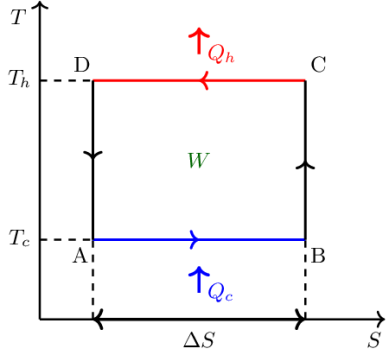
Figure 1: Bath temperature $T$-system entropy $S$ diagram of the considered Carnot heat pump cycle. The red (blue) horizontal line denotes the hot (cold) isotherm. The black vertical lines depict the adiabats. Per cycle, the input work $W$ is consumed to pump the heat $Q_{c}$ from the cold bath at temperature $T_{c}$ and deliver the heat $Q_{h}=Q_{c}+W$ into the hot bath at temperature $T_{h}$.

In the low-dissipation (LD) regime [14, 63, 64], $Q_{i}$, $i=c,h$ assume the form

$$Q_{c} = T_{c}\Delta S-\frac{\sigma_{c}}{t_{c}},$$ (2)

$$Q_{h} = T_{h}\Delta S+\frac{\sigma_{h}}{t_{h}},$$ (3)

where the positive irreversibility parameters $\sigma_{i}$ depend on the details of system construction, and $t_{i}$ are durations of the two isotherms. $\Delta S$ denotes the increase (decrease) in the entropy of the system during the cold (hot) isotherm. The corresponding contributions to $Q_{c}$ and $Q_{h}$ are reversible, i.e., they do not contribute to the total entropy produced per cycle,

$$\Delta S_{tot}=-\frac{Q_{c}}{T_{c}}+\frac{Q_{h}}{T_{h}}=\frac{\sigma_{c}}{t_{c}T_{c}}+\frac{\sigma_{h}}{t_{h}T_{h}}\geq 0.$$ (4)

$\Delta S_{tot}$ is solely determined by the irreversible contributions, proportional to the irreversibility parameters, and vanishes both in the quasi-static limit, $t_{h}\to\infty$ and $t_{c}\to\infty$, and in the quilibrium limit, $\sigma_{c}=\sigma_{h}=0$. The LD forms (2) and (3) of the transferred heats can be quite generally considered as first-order expansions of the exact expressions in the inverse durations of the isotherms [65, 66, 67, 68, 69, 63]. Besides, the LD model is exact for optimized overdamped Brownian heat engines [27, 1] and other specific scenarios [70, 66].

We assume that durations of the adiabatic branches are proportional to durations of the isotherms so that the cycle time is given by $t_{p}=a(t_{h}+t_{c})$. Since the constant $a\geq 1$ only affects the heating load of the pump (see Eq. (5) below), we assume in the rest of the paper that $a=1$. This value corresponds to infinitely fast adiabats [71] and thus maximum heating load as a function of $a$.

III Heating load and COP

The performance of heat devices is described by their power, $P$, and efficiency, $\epsilon$. For heat pumps, $P$ and $\epsilon$ are called the coefficient of performance (COP) and the heating load [72, 60]. $P$ measures the average heat pumped into the hot bath per unit time, and $\epsilon$ shows how much work is needed to pump 1 Joule of heat to the hot body.

Using Eqs. (2) and (3) together with the first law of thermodynamics, $W=Q_{h}-Q_{c}$, the heating load and COP of the LD heat pump can be expressed as

$$P = \frac{Q_{h}}{t_{p}}=\frac{T_{h}\Delta S}{t_{p}}+\frac{\sigma_{h}}{t_{h}t_{p}},$$ (5)

$$\epsilon = \frac{Q_{h}}{W}=\frac{\epsilon_{C}}{1+T_{c}\epsilon_{C}\Delta S_{tot}/(Pt_{p})}.$$ (6)

The maximum (Carnot) COP, $\epsilon=\epsilon_{C}$, is attained under reversible conditions ($\Delta S_{tot}=0$). The minimum COP, $\epsilon=1$, describes the situation when no heat is pumped from the cold bath and thus the delivered heat, $Q_{h}$, equals the input work, $W$. In this regime, heat pumps are not better than work-to-heat converters, such as resistance heating wires. In the next section, we study COP at maximum heating load for LD heat pumps.

IV COP at maximum heating load

Most of the available expressions for maximum efficiency at a fixed power for various models [57, 54, 55, 56, 51, 58, 30, 16, 40, 59] are given as functions of the dimensionless variable $P/P^{*}$, measuring loss in power, $P$, with respect to the maximum power, $P^{*}$. This normalization of power usually significantly simplifies the resulting expressions. However, for endoreversible heat pumps [41, 42] the maximum power diverges, suggesting that such a normalization might, in our case, not be possible. Indeed, we show below that $P^{*}\to\infty$ also for LD heat pumps.

To introduce a meaningful dimensionless heating load, we define the reduced heats and durations as

$$\tilde{Q}_{i}=\frac{Q_{i}}{T_{h}\Delta S},~{}\tilde{t}_{i}=\frac{T_{h}\Delta S}{\sigma_{h}}t_{i},\quad i=c,h.$$ (7)

Using Eqs. (2) and (3), the reduced heats read

$$\tilde{Q}_{c} = \frac{\epsilon_{C}-1}{\epsilon_{C}}-\frac{1}{\sigma(1-\alpha)\tilde{t}_{p}}.$$ (8)

$$\tilde{Q}_{h} = 1+\frac{1}{\alpha\tilde{t}_{p}}.$$ (9)

Here, $\sigma=\sigma_{h}/\sigma_{c}$ is the so-called irreversibility ratio, $\tilde{t}_{p}=\tilde{t}_{h}+\tilde{t}_{c}$ denotes the reduced cycle duration, and $\alpha\equiv t_{h}/t_{p}$ measures the allocation of the cycle duration between the two isotherms. We define the reduced heating load as the ratio of the reduced heat to the reduced cycle duration:

$$\tilde{P}=\frac{\tilde{Q}_{h}}{\tilde{t}_{p}}=\frac{1}{\tilde{t}_{p}}+\frac{1}{\alpha\tilde{t}_{p}^{2}}=\frac{\sigma_{h}}{(T_{h}\Delta S)^{2}}P.$$ (10)

The reduced heating load is a monotonically decreasing function of both $\alpha$ and $\tilde{t}_{p}$. The inequality $Q_{h}>Q_{c}>0$, following from the requirement that the considered device pumps heat from the cold to the hot bath, restricts the minimal reduced cycle duration as

$$\tilde{t}_{p}>\frac{\epsilon_{C}}{\sigma(\epsilon_{C}-1)(1-\alpha)}.$$ (11)

The maximum reduced heating load, $\tilde{P}^{*}$, attained for the minimal allowed values of $\alpha$ and $\tilde{t}_{p}$,

$$\alpha^{*} = 0,$$ (12)

$$\tilde{t}_{p}^{*} = \frac{\epsilon_{C}}{\sigma(\epsilon_{C}-1)},$$ (13)

hence diverges. The corresponding COP is most easily obtained from the formula $\epsilon=\tilde{Q}_{h}/(\tilde{Q}_{h}-\tilde{Q}_{c})$. Altogether, the maximum reduced heating load and the corresponding COP read

$$\tilde{P}^{*} = \infty,$$ (14)

$$\epsilon^{*} = 1.$$ (15)

This performance is achieved whenever the hot isotherm is much faster than the cold one and thus $\alpha=\alpha^{*}\to 0$. Noteworthy, the COP at maximum power is the smallest possible, corresponding to the negligible amount of heat pumped from the cold bath compared to the input work, $\tilde{Q}_{h}=\tilde{W}+\tilde{Q}_{c}\gg\tilde{Q}_{c}$. A heat pump operating at the maximum heating load thus works as an electric heater transforming work in the form of electric energy into heat. Practical heat pumps should not operate anywhere close to this regime. In the next section, we uncover more practical operation regimes of LD heat pumps by deriving their maximum COP at a given heating load.

V Maximum COP at given heating load

Fixing the reduced heating load in Eq. (10) creates the dependency

$$\alpha=\frac{1}{\tilde{t}_{p}(\tilde{P}\tilde{t}_{p}-1)}$$ (16)

between $\alpha\in[0,1]$ and $\tilde{t}_{p}$. Substituting Eq. (16) into Eqs. (8) and (9) and using the condition $\tilde{Q}_{h}>\tilde{Q}_{c}>0$, we find the inequality

$$\tilde{t}_{p}>\frac{1+\tilde{P}\tilde{t}^{*}_{p}}{2\tilde{P}}+\sqrt{\left(\frac{1+\tilde{P}\tilde{t}^{*}_{p}}{2\tilde{P}}\right)^{2}+\frac{1-\tilde{t}^{*}_{p}}{\tilde{P}}}\equiv\tilde{t}_{p,min}.$$ (17)

The minimum value of the reduced cycle duration for fixed heating load, $\tilde{t}_{p,min}$, thus depends on the irreversibility ratio $\sigma$ and the Carnot COP $\epsilon_{C}$ via $\tilde{t}_{p}^{*}$ in Eq. (13). For maximum and minimum values of $\sigma$, $\tilde{t}_{p,min}$ reads

$$\tilde{t}_{p,min}=\begin{cases}\frac{1+\sqrt{1+4\tilde{P}}}{2\tilde{P}}&\text{for}\quad\sigma\to\infty\\ \infty&\text{for}\quad\sigma\to 0\end{cases}.$$ (18)

The COP (6) can be written in terms of the reduced parameters introduced above as

$$\epsilon=\left[1+\frac{\tilde{P}\tilde{t}_{p}-1}{\sigma\tilde{P}\tilde{t}_{p}(\tilde{P}\tilde{t}_{p}^{2}-\tilde{t}_{p}-1)}-\frac{\epsilon_{C}-1}{\tilde{P}\tilde{t}_{p}\epsilon_{C}}\right]^{-1}.$$ (19)

Below we will find its maximum as a function of $\tilde{t}_{p}>\tilde{t}_{p,min}$.

V.1 Bounds

First, we determine the upper and lower bounds on the maximum COP at a given heating load. Taking the derivative of $\epsilon$ (19) with respect to $\sigma$, one finds that $\partial\epsilon/\partial\sigma>0$ and thus $\epsilon$ monotonically increases with $\sigma$. Physically, this is because the COP in Eq. (6) is for a fixed $P$ and $\sigma_{h}$ (fixed by our choice of time unit) a monotonically decreasing function of the entropy production, $\Delta S_{tot}$, and thus $\sigma_{c}$. The lower bound on COP (19) for a fixed $P$ is thus attained if the irreversible losses during the hot isotherm are negligible compared to those during the cold one ($\sigma=\sigma_{h}/\sigma_{c}\to 0$). The corresponding COP equals 1. Note that due to the condition (17) the reduced cycle duration $\tilde{t}_{p}$ in this regime diverges [cf. Eq. (18)].

The upper bound on COP (19) for a fixed $P$ is attained if irreversible losses during the cold isotherm are negligible compared to those during the hot one ($\sigma\to\infty$). In this regime, the COP,

$$\epsilon=\left(1-\frac{\epsilon_{C}-1}{\tilde{P}\tilde{t}_{p}\epsilon_{C}}\right)^{-1},$$ (20)

monotonically decreases with $\tilde{t}_{p}$ and thus it attains its maximum for $\tilde{t}_{p}=\tilde{t}_{p,min}=\left(1+\sqrt{1+4\tilde{P}}\right)/(2\tilde{P})$. Altogether, the bounds on the maximum COP at given heating load, $\epsilon^{opt}=\epsilon^{opt}(\tilde{P})$, are given by

$$1\leq\epsilon^{opt}\leq\frac{(1+\sqrt{1+4\tilde{P}})\epsilon_{C}}{2-(1-\sqrt{1+4\tilde{P}})\epsilon_{C}}\equiv\epsilon^{opt}_{>}.$$ (21)

As expected, the upper bound, $\epsilon^{opt}_{>}$, converges to $\epsilon_{C}$ for $\tilde{P}\to 0$ and to 1 for $\tilde{P}\to\infty$.

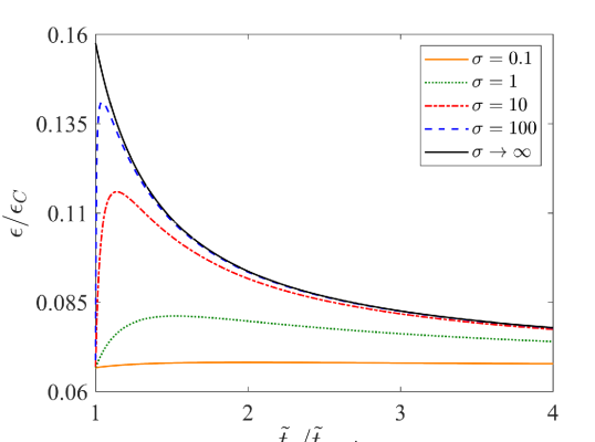
Figure 2: COP (19) as a function of $\tilde{t}_{p}/\tilde{t}_{p,min}$ (17) for different values of $\sigma$, $\tilde{P}=1$, and $\epsilon_{C}=15$. The figure shows that the upper bound (21) on the optimal COP is obtained for $\sigma\to\infty$.

V.2 Arbitrary parameters

Outside the limiting regimes discussed in the previous section, the optimization of COP (19) for a fixed $P$ is more complicated. In Fig. 2, we show $\epsilon$ as a function of $\tilde{t}_{p}/\tilde{t}_{p,min}$ for five values of $\sigma$. The black solid line for $\sigma\to\infty$ indeed monotonously decreases with $\tilde{t}_{p}$. However, for an arbitrary finite $\sigma$, the COP exhibits a global maximum for $\tilde{t}_{p}^{opt}>\tilde{t}_{p,min}$. Its position follows from the condition $\partial\epsilon/\partial\tilde{t}_{p}|_{\tilde{t}_{p}=\tilde{t}_{p}^{opt}}=0$, which implies the quartic equation

$$\tilde{t}_{p}^{4}+a\tilde{t}_{p}^{3}+b\tilde{t}_{p}^{2}+c\tilde{t}_{p}+\frac{c}{2}=0,\quad\tilde{t}_{p}=\tilde{t}_{p}^{opt},$$ (22)

with the coefficients

$$\left(\begin{array}[]{c}a\\ b\\ c\end{array}\right)=\frac{1}{\tilde{P}^{2}}\left(\begin{array}[]{c}-2\tilde{P}-2\tilde{P}^{2}\tilde{t}_{p}^{*}\\ 1-2\tilde{P}+4\tilde{P}\tilde{t}_{p}^{*}\\ 2-2\tilde{t}_{p}^{*}\end{array}\right).$$ (23)

Eq. (22) has four roots which can be determined analytically using Ferrari's method. The optimal reduced cycle duration is given by the largest real-valued root:

$$\tilde{t}^{opt}_{p}(\tilde{P},\tilde{t}_{p}^{*})=-\frac{a}{4}+F+\frac{1}{2}\sqrt{-2C-4F^{2}-\frac{D}{F}},$$ (24)

where

$$A =b^{2}+3c(2-a),$$ (25)

$$B =2b^{3}-9bc(4+a)+\frac{27c}{2}(a^{2}+2c),$$ (26)

$$C =b-\frac{3a^{2}}{8},$$ (27)

$$D =\frac{a^{3}}{8}-\frac{ab}{2}+c,$$ (28)

$$E =\sqrt[3]{\frac{B+\sqrt{B^{2}-4A^{3}}}{2}},$$ (29)

$$F =\frac{\sqrt{3}}{6}\sqrt{\frac{A}{E}+E-2C}.$$ (30)

For a fixed $\tilde{P}$, the reduced optimal cycle duration only depends on $\tilde{t}_{p}^{*}$ in Eq. (13). Inserting $\tilde{t}^{opt}_{p}$ into Eq. (19) yields the maximum COP at given heating load for the LD heat pump, $\epsilon^{opt}=\epsilon^{opt}(\tilde{P},\sigma,\epsilon_{C})$.

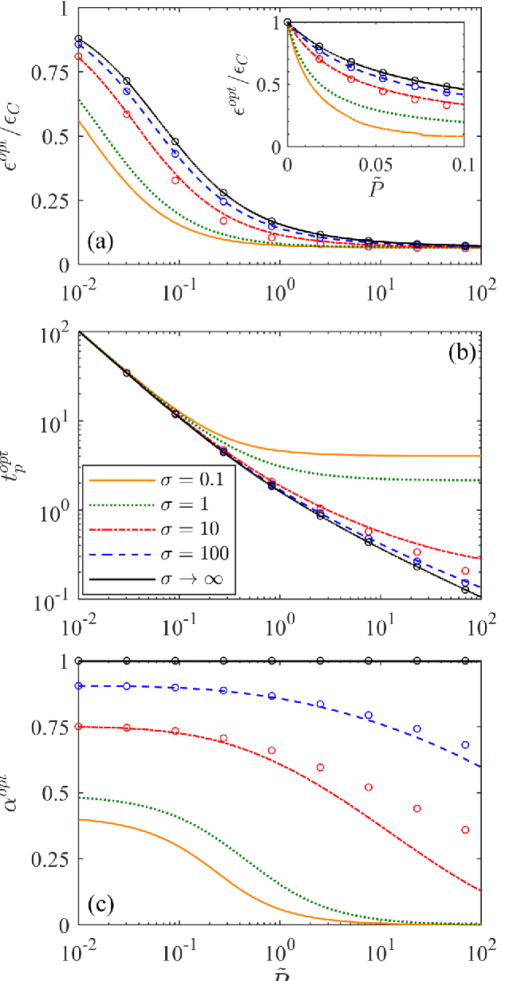
Figure 3: The optimal COP (a), the corresponding reduced cycle duration (b), and its allocation between hot and cold isotherms (c) as a function of $\tilde{P}$ for different values of $\sigma$ and $\epsilon_{C}=15$. The circles follow from the approximate expressions (31) and (32). The lines were obtained using the exact result (24).

In Fig. 3, we show $\epsilon^{opt}$, $\tilde{t}^{opt}_{p}$, and $\alpha^{opt}=[\tilde{t}^{opt}_{p}(\tilde{P}\tilde{t}^{opt}_{p}-1)]^{-1}$ [see Eq. (16)] as functions of $\tilde{P}$ for five values of $\sigma$. The exact theoretical results are depicted by solid lines. We checked that they agree within numerical precision with the optimal COP obtained by the direct numerical maximization of $\epsilon$ in Eq. (19). In agreement with the inequalities (21), $\epsilon^{opt}$ in Fig. 3(a) converges to 1 for $\tilde{P}\to\infty$ and to $\epsilon_{C}$ for $\tilde{P}\to 0$ (see the inset) for all $\sigma$. This panel also shows the monotonic increase of $\epsilon^{opt}$ with $\sigma$ discussed in Sec. V.1. The increase of the maximum COP with decreasing heating load for large $\tilde{P}$ is very slow, showing that reasonably efficient heat pumps has to operate at small values of $\tilde{P}$. In this respect, heat pumps qualitatively differ from heat engines and refrigerators, which exhibit large gains in efficiency when their power is slightly decreased from its maximum value [58, 16].

The $\sigma$-dependency of $\tilde{t}_{p}^{opt}$ in Fig. 3(b) is significant for small values of $\sigma$ but negligible for large $\sigma$. Even though the $\sigma$-dependency of $\alpha^{opt}$ in Fig. 3(c) is always significant, the COP in Eq. (19) no longer depends on $\alpha$. This suggests that we might obtain an analytically tractable approximation for $\epsilon^{opt}$, valid for intermediate and large values of $\sigma$, by expanding $\tilde{t}_{p}^{opt}$ in powers of $\tilde{t}_{p}^{*}\sim 1/\sigma$. Up to the leading order in $\tilde{t}_{p}^{*}$, we find

$$\tilde{t}_{p}^{opt} \approx \frac{1+\sqrt{1+4\tilde{P}}}{2\tilde{P}}+\frac{\sqrt{\tilde{t}_{p}^{*}}}{(1+4\tilde{P})^{1/4}},$$ (31)

$$\epsilon^{opt} \approx \epsilon_{>}^{opt}-\frac{8\tilde{P}(1-\epsilon_{C}^{-1})(\epsilon_{>}^{opt})^{2}\sqrt{\tilde{t}_{p}^{*}}}{(1+4\tilde{P})^{1/4}(1+\sqrt{1+4\tilde{P}})^{2}}.$$ (32)

The corrections to these formulas are proportional to $\tilde{t}_{p}^{*}$. For large values of $\tilde{t}_{p}^{*}$, the approximation (32) leads to negative (thus unphysical) COP. Circles in Fig. 3 show the predictions from the approximate formulas for $\sigma>1$, when the approximate $\epsilon^{opt}>0$. For large values of $\sigma$ (small $\tilde{t}_{p}^{*}$), the approximate (circles) and exact (lines) results indeed perfectly overlap.

VI Comparison with endoreversible heat pumps

Let us now compare the obtained results on maximum COP at a given heating load of LD heat pumps to the corresponding known results for endoreversible heat pumps [42, 61, 62]. The endoreversible thermodynamics assumes that the working fluid of thermal devices operates reversibly. The only considered sources of entropy production are the finite-time heat transfers between thermal reservoirs and the working fluid [73, 74, 75]. LD models generally describe the thermodynamics of slowly driven systems [14, 63, 64]. On the other hand, up to a few exceptions [76, 77, 78], the endoreversible models are usually phenomenological [75, 79, 10, 11, 80].

The works [42, 61] on the maximum COP at a given heating load of endoreversible heat pumps assume that the heat transfers between the working fluid and baths obey Newton's law of cooling. Denoting the temperatures of the working fluid during the hot and cold isotherm by $T_{hw}$ and $T_{cw}$ and the corresponding heat conductivities as $\kappa_{h}$ and $\kappa_{c}$, the heats transferred during the isotherms are in this case given by

$$Q_{h} = \kappa_{h}t_{h}(T_{hw}-T_{h}),$$ (33)

$$Q_{c} = \kappa_{c}t_{c}(T_{c}-T_{cw}).$$ (34)

More general heat transfer laws used in Ref. [62] lead to qualitatively the same results as Newton's law of cooling, to which we stick in the following discussion.

In the endorevesible models, the COP $\varepsilon_{en}=Q_{h}/(Q_{h}-Q_{c})$ is maximized with respect to the temperatures of the working fluid $T_{hw}$ and $T_{cw}$. The ratio $t_{h}/t_{c}$ of the durations of the two isotherms is determined by the endoreversibility requirement $Q_{h}/T_{hw}-Q_{c}/T_{cw}=0$ and the total cycle duration does not influence the resulting expressions. Performing the maximisation for a fixed heating load $P=Q_{h}/(t_{h}+t_{c})$ with the definitions (33) and (34) yields the maximum COP [42, 62]

$$\epsilon^{opt}_{en}=1+\frac{\epsilon_{C}-1}{1+\epsilon_{C}P\left(1+\sqrt{r}\right)^{2}/(\kappa_{h}T_{h})},$$ (35)

where $r=\kappa_{h}/\kappa_{c}$. The maximum COP at fixed heating load thus behaves qualitatively in the same way as the corresponding result for LD heat pumps: $\epsilon^{opt}_{en}$ converges to $\epsilon_{C}$ for $P\to 0$ and to $1$ for $P\to\infty$. However, the precise functional forms of the maximum COP for LD and endoreversible heat pumps in general differ. The exception is the parameter regime

$$\tilde{t}_{p}^{*}=1,\quad\frac{(1+\sqrt{r})^{2}}{\kappa_{h}}=\frac{4\sigma_{h}}{T_{h}\Delta S^{2}},$$ (36)

when the expressions for $\epsilon^{opt}_{en}$ and $\epsilon^{opt}$ are identical. In this regime, one can thus find an exact mapping between the LD and the endoreversible model. Note that for $\tilde{t}_{p}^{*}=1$, Eq. (22) reduces to a quadratic equation, and Eq. (13) implies $\sigma_{h}/T_{h}=\sigma_{c}/T_{c}$.

One way to show that the two models are equivalent only in the parameter regime (36) is to compare the formulas for $\epsilon^{opt}_{en}$ and $\epsilon^{opt}$ in the limiting regimes, where they become simple. To this end, we expand the two maximum COPs as functions of the heating load close to infinite and close to vanishing $P$. Up to the leading order in $P$, the expansions read

$$\epsilon^{opt} \approx 1+\frac{1-\epsilon_{C}^{-1}}{4\tilde{t}_{p}^{*}}\frac{(T_{h}\Delta S)^{2}}{\sigma_{h}P},$$ (37)

$$\epsilon^{opt}_{en} \approx 1+\frac{1-\epsilon_{C}^{-1}}{\left(1+\sqrt{r}\right)^{2}}\frac{\kappa_{h}T_{h}}{P},$$ (38)

and

$$\epsilon^{opt} \approx \epsilon_{C}-\epsilon_{C}(\epsilon_{C}-1)\left(1+\sqrt{\tilde{t}_{p}^{*}}\right)^{2}\frac{\sigma_{h}P}{(T_{h}\Delta S)^{2}}$$ (39)

$$\epsilon^{opt}_{en} \approx \epsilon_{C}-\epsilon_{C}(\epsilon_{C}-1)\left(1+\sqrt{r}\right)^{2}\frac{P}{\kappa_{h}T_{h}}.$$ (40)

The corrections to Eqs. (37) and (38) are proportional to $1/P^{2}$ and those to (39) and (40) are proportional to $P^{2}$. The LD and endoreversible models for heat pumps can be mapped to each other only if the two types of expansions agree, leading to the conditions

$$\frac{(1+\sqrt{r})^{2}}{\kappa_{h}} = \frac{\sigma_{h}}{T_{h}\Delta S^{2}}4\tilde{t}_{p}^{*},$$ (41)

$$\frac{(1+\sqrt{r})^{2}}{\kappa_{h}} = \frac{\sigma_{h}}{T_{h}\Delta S^{2}}\left(1+\sqrt{\tilde{t}_{p}^{*}}\right)^{2}.$$ (42)

The first equality follows from Eqs. (37) and (38) and the second one from Eqs. (39) and (40). Requiring validity of both yields the condition (36) (see Appendix A for more details). In Fig. 4, we show $\epsilon^{opt}$ and $\epsilon^{opt}_{en}$ as functions of the reduced heating load $\tilde{P}$. The marked lines show the agreement of $\epsilon^{opt}$ and $\epsilon^{opt}_{en}$ when Eq. (36) holds and thus $\tilde{t}^{*}_{p}=1$. The remaining lines show $\epsilon^{opt}$ (green dashed line) and $\epsilon^{opt}_{en}$ for parameters obeying solely Eq. (41) (blue dotted line) and (42) (red dash-dotted line) for $\tilde{t}^{*}_{p}=3/14$. As expected, the green dashed line only agrees with the blue dotted line for large values of $\tilde{P}$ and with the red dash-dotted line for small values of $\tilde{P}$.

We tested that also the LD and endoreversible models for heat engines and refrigerators lead to identical results when Eq. (36) holds (data not shown). Besides, an equivalent condition was derived in the linear response regime for heat engines operating at maximum power [53, 52].

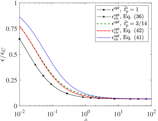
Figure 4: The maximum COPs at fixed heating load for LD ($\epsilon^{opt}$) and endoreversible ($\epsilon^{opt}_{en}$) heat pumps as functions of $\tilde{P}$ for $\epsilon_{C}=15$ and $\sigma_{h}/(T_{h}\Delta S)^{2}=1/(\kappa_{h}T_{h})$. The marked black solid lines show that the condition (36) implies $\epsilon^{opt}=\epsilon^{opt}_{en}$. For the remaining lines, we set $\sigma=5$ and thus $\tilde{t}^{*}_{p}=3/14$. The blue dotted line corresponds to $r$ obtained from Eq. (41). For the red dash-dotted line, we calculated $r$ using Eq. (42).

VII Conclusion and Outlook

Like endoreversible heat pumps, Carnot-type low-dissipation (LD) heat pumps operate at maximum power as work to heat converters such as standard electric heaters. Practical heat pumps thus should not operate in this regime. To provide a tool to decide a suitable regime of operation for a given application, we derived an analytical expression for maximum efficiency at a given heating load for LD heat pumps. Besides, we derived upper and lower bounds on this quantity. Qualitatively, our results agree with the corresponding findings obtained earlier for endoreversible heat pumps. Unlike the phenomenological endoreversible models, LD models represent a general first-order finite-time correction to the reversible operation and thus their parameters can be either calculated using a perturbation analysis or measured in experiments. Furthermore, the derived upper bound on the maximum efficiency can be considered as a loose upper bound on the efficiency of heat pumps in general. By adding the result for heat pumps to the known formulas for LD heat engines and refrigerators [58, 16, 59], the present paper completes the collection of results for maximum efficiency at a given power for LD thermal devices.

The presented result for maximum efficiency at a given heating load depends on the reduced heating load $\tilde{P}$ in Eq. (10). Therefore, the heating load can be further optimized for the chosen unit of energy flux without affecting the corresponding maximum efficiency. Such optimization tasks performed for LD heat engines and refrigerators are described in Refs. [81, 82]. Besides, it would be interesting to investigate the operation regime of maximum efficiency at given power for LD thermal devices concerning its dynamical stability [15, 83, 84, 85]. Finally, it would be worth to investigate maximum efficiency at given power for heat devices operating between finite-sized heat sources [86, 19, 87, 88, 89, 90] and compare the results to those derived using the idealized LD models. For heat engines working with two finite-sized reservoirs, the maximum efficiency at given power has been derived in Ref. [90].

Appendix A Heat flows in the parameter regime (36)

In this Appendix, we investigate the physical significance of the parameter regime (36), leading to the same expressions for $\epsilon^{opt}_{en}$ and $\epsilon^{opt}$ for the endoreversible and LD models. As the average heat flows $Q_{h}/t_{p}$ are for the two models fixed to be the same value of power $P$, we focus on the structure of the average heat flows $Q_{c}/t_{p}$.

For the endoreversible heat pump, combining Eqs. (33) and (34), together with the endoreversibility condition $Q^{en}_{h}/T_{hw}-Q^{en}_{c}/T_{cw}=0$ yields (here and below we use the superscript en to distinguish between the heats for the endoreversible and LD models)

$$\frac{Q_{c}^{en}}{t_{p}}=\frac{T_{c}P[P+\kappa_{h}(T_{h}-T_{hw})]}{rP(T_{h}-T_{hw})+T_{hw}[P+\kappa_{h}(T_{h}-T_{hw})]}.$$ (43)

For the LD heat pump, inserting Eq. (16) into Eq. (8) implies

$$\frac{Q_{c}}{t_{p}}=\frac{T_{c}T_{h}\Delta S^{2}}{\sigma_{h}}\frac{\tilde{P}\tilde{t}_{p}^{2}-\tilde{t}_{p}(1+\tilde{P}\tilde{t}_{p}^{*})+\tilde{t}_{p}^{*}-1}{\tilde{t}_{p}(\tilde{P}\tilde{t}_{p}^{2}-\tilde{t}_{p}-1)}.$$ (44)

Imposing the condition (36) and returning to dimensional power (10), the heat flow for the LD model changes to

$$\frac{Q_{c}}{t_{p}}=\frac{4\kappa_{h}T_{c}}{\left(\sqrt{r}+1\right)^{2}}\frac{P\left(\sqrt{r}+1\right)^{2}(\tilde{t}_{p}-1)-4\kappa_{h}T_{h}}{P\left(\sqrt{r}+1\right)^{2}\tilde{t}_{p}^{2}-4\kappa_{h}T_{h}(\tilde{t}_{p}+1)}.$$ (45)

Interestingly, the functional forms of the heat flows (43) and (45) in terms of power $P$ and the parameter to be optimized ($T_{hw}$ for the endoreversible and $\tilde{t}_{p}$ for the LD model) are different, even though the analysis in the main text proves that they must be the same functions of power when $T_{hw}$ and $t_{p}$ are substituted by the values

$$T_{hw} = T_{h}+\frac{(1+\sqrt{r})P}{\kappa_{h}},$$ (46)

$$\tilde{t}_{p} = 2+\frac{4\kappa_{h}T_{h}}{\left(\sqrt{r}+1\right)^{2}P},$$ (47)

maximizing the two heat flows and thus, for fixed power, also the COP (6). The formulas for the two heat flows remain different even after the substitutions $T_{hw}=(1+\sqrt{r})T/\kappa_{h}$ and $\tilde{t}_{p}=2+4\kappa_{h}T_{h}/[\left(\sqrt{r}+1\right)^{2}T]$, which lead to expressions $\tilde{Q}^{en}_{c}(T,P)/t_{p}$ and $\tilde{Q}_{c}(T,P)/t_{p}$ exhibiting the same maximum,

$$\frac{\tilde{Q}^{en}_{c}}{t_{p}}=\frac{\tilde{Q}_{c}}{t_{p}}=\frac{\kappa_{h}T_{c}P}{\kappa_{h}T_{h}+P(1+\sqrt{r})^{2}},$$ (48)

for the same value of $T=P$. The expressions $\tilde{Q}^{en}_{c}(T,P)/t_{p}$ and $\tilde{Q}_{c}(T,P)/t_{p}$ are thus different unless $T=P$. We conclude that there is no deep physical reason why the performances of the optimized endoreversible and LD models are the same in the parameter regime (36).

References

- Holubec and Ryabov [2015] V. Holubec and A. Ryabov, Efficiency at and near maximum power of low-dissipation heat engines, Phys. Rev. E 92, 052125 (2015).
- Ammar et al. [2019] A. Ammar, K. Sopian, M. Alghoul, B. Elhub, and A. Elbreki, Performance study on photovoltaic/thermal solar-assisted heat pump system, J. Therm. Anal. Calorim. 136, 79 (2019).
- Chua et al. [2010] K. J. Chua, S. K. Chou, and W. Yang, Advances in heat pump systems: A review, Appl. Energy 87, 3611 (2010).
- Mohanraj et al. [2021] M. Mohanraj, L. Karthick, and R. Dhivagar, Performance and economic analysis of a heat pump water heater assisted regenerative solar still using latent heat storage, Appl. Therm. Eng. 196, 117263 (2021).
- Hu and Yuill [2021] Y. Hu and D. P. Yuill, Effects of multiple simultaneous faults on characteristic fault detection features of a heat pump in cooling mode, Energy Build. , 111355 (2021).
- Aye et al. [2010] L. Aye, R. Fuller, and A. Canal, Evaluation of a heat pump system for greenhouse heating, Int. J. Therm. Sci. 49, 202 (2010).
- Hong and Howarth [2016] B. Hong and R. W. Howarth, Greenhouse gas emissions from domestic hot water: heat pumps compared to most commonly used systems, Energy Sci. Eng. 4, 123 (2016).
- Holubec and Ryabov [2017] V. Holubec and A. Ryabov, Diverging, but negligible power at carnot efficiency: Theory and experiment, Phys. Rev. E 96, 062107 (2017).
- Gordon and Orlov [1993] J. Gordon and V. N. Orlov, Performance characteristics of endoreversible chemical engines, J. Appl. Phys. 74, 5303 (1993).
- Rubin and Andresen [1982] M. H. Rubin and B. Andresen, Optimal staging of endoreversible heat engines, J. Appl. Phys. 53, 1 (1982).
- Chen and Yan [1989a] J. Chen and Z. Yan, Unified description of endoreversible cycles, Phys. Rev. A 39, 4140 (1989a).
- Apertet et al. [2013] Y. Apertet, H. Ouerdane, A. Michot, C. Goupil, and P. Lecoeur, On the efficiency at maximum cooling power, EPL 103, 40001 (2013).
- Hu et al. [2013] Y. Hu, F. Wu, Y. Ma, J. He, J. Wang, A. C. Hernández, and J. M. M. Roco, Coefficient of performance for a low-dissipation carnot-like refrigerator with nonadiabatic dissipation, Phys. Rev. E 88, 062115 (2013).
- Esposito et al. [2010a] M. Esposito, R. Kawai, K. Lindenberg, and C. Van den Broeck, Efficiency at maximum power of low-dissipation carnot engines, Phys. Rev. Lett. 105, 150603 (2010a).
- Gonzalez-Ayala et al. [2020] J. Gonzalez-Ayala, J. Guo, A. Medina, J. Roco, and A. C. Hernández, Energetic self-optimization induced by stability in low-dissipation heat engines, Phys. Rev. Lett. 124, 050603 (2020).
- Holubec and Ye [2020] V. Holubec and Z. Ye, Maximum efficiency of low-dissipation refrigerators at arbitrary cooling power, Phys. Rev. E 101, 052124 (2020).
- Hernández et al. [2015] A. C. Hernández, A. Medina, and J. Roco, Time, entropy generation, and optimization in low-dissipation heat devices, New J. Phys. 17, 075011 (2015).
- Benenti et al. [2011] G. Benenti, K. Saito, and G. Casati, Thermodynamic bounds on efficiency for systems with broken time-reversal symmetry, Phys. Rev. Lett. 106, 230602 (2011).
- Izumida and Okuda [2014] Y. Izumida and K. Okuda, Work output and efficiency at maximum power of linear irreversible heat engines operating with a finite-sized heat source, Phys. Rev. Lett. 112, 180603 (2014).
- Van den Broeck [2005] C. Van den Broeck, Thermodynamic efficiency at maximum power, Phys. Rev. Lett. 95, 190602 (2005).
- Izumida et al. [2015] Y. Izumida, K. Okuda, J. Roco, and A. C. Hernández, Heat devices in nonlinear irreversible thermodynamics, Phys. Rev. E 91, 052140 (2015).
- Izumida and Okuda [2012] Y. Izumida and K. Okuda, Efficiency at maximum power of minimally nonlinear irreversible heat engines, EPL 97, 10004 (2012).
- Izumida et al. [2013] Y. Izumida, K. Okuda, A. C. Hernández, and J. Roco, Coefficient of performance under optimized figure of merit in minimally nonlinear irreversible refrigerator, EPL 101, 10005 (2013).
- Uzdin and Kosloff [2014] R. Uzdin and R. Kosloff, Universal features in the efficiency at maximal work of hot quantum otto engines, EPL 108, 40001 (2014).
- Abah et al. [2012] O. Abah, J. Rossnagel, G. Jacob, S. Deffner, F. Schmidt-Kaler, K. Singer, and E. Lutz, Single-ion heat engine at maximum power, Phys. Rev. Lett. 109, 203006 (2012).
- Roßnagel et al. [2014] J. Roßnagel, O. Abah, F. Schmidt-Kaler, K. Singer, and E. Lutz, Nanoscale heat engine beyond the carnot limit, Phys. Rev. Lett. 112, 030602 (2014).
- Schmiedl and Seifert [2007] T. Schmiedl and U. Seifert, Efficiency at maximum power: An analytically solvable model for stochastic heat engines, EPL 81, 20003 (2007).
- Segal [2008] D. Segal, Stochastic pumping of heat: Approaching the carnot efficiency, Phys. Rev. Lett. 101, 260601 (2008).
- Jarzynski and Mazonka [1999] C. Jarzynski and O. Mazonka, Feynman’s ratchet and pawl: An exactly solvable model, Phys. Rev. E 59, 6448 (1999).
- Dechant et al. [2017] A. Dechant, N. Kiesel, and E. Lutz, Underdamped stochastic heat engine at maximum efficiency, EPL 119, 50003 (2017).
- Holubec [2014] V. Holubec, An exactly solvable model of a stochastic heat engine: optimization of power, power fluctuations and efficiency, J. Stat. Mech. 2014, P05022 (2014).
- Esposito et al. [2009] M. Esposito, K. Lindenberg, and C. Van den Broeck, Universality of efficiency at maximum power, Phys. Rev. Lett. 102, 130602 (2009).
- Sheng and Tu [2014] S. Sheng and Z. C. Tu, Weighted reciprocal of temperature, weighted thermal flux, and their applications in finite-time thermodynamics, Phys. Rev. E 89, 012129 (2014).
- Sheng and Tu [2015] S. Sheng and Z. C. Tu, Constitutive relation for nonlinear response and universality of efficiency at maximum power for tight-coupling heat engines, Phys. Rev. E 91, 022136 (2015).
- Ye et al. [2017] Z. Ye, Y. Hu, J. He, and J. Wang, Universality of maximum-work efficiency of a cyclic heat engine based on a finite system of ultracold atoms, Sci. Rep. 7, 1 (2017).
- Guo et al. [2013] J. Guo, J. Wang, Y. Wang, and J. Chen, Universal efficiency bounds of weak-dissipative thermodynamic cycles at the maximum power output, Phys. Rev. E 87, 012133 (2013).
- Esposito et al. [2010b] M. Esposito, R. Kawai, K. Lindenberg, and C. Van den Broeck, Quantum-dot carnot engine at maximum power, Phys. Rev. E 81, 041106 (2010b).
- Allahverdyan et al. [2008] A. E. Allahverdyan, R. S. Johal, and G. Mahler, Work extremum principle: Structure and function of quantum heat engines, Phys. Rev. E 77, 041118 (2008).
- Allahverdyan et al. [2013] A. E. Allahverdyan, K. V. Hovhannisyan, A. V. Melkikh, and S. G. Gevorkian, Carnot cycle at finite power: Attainability of maximal efficiency, Phys. Rev. Lett. 111, 050601 (2013).
- Long et al. [2018] R. Long, Z. Liu, and W. Liu, Performance analysis for minimally nonlinear irreversible refrigerators at finite cooling power, Phys. A: Stat. Mech. Appl. 496, 137 (2018).
- Leff and Teeters [1978] H. S. Leff and W. D. Teeters, Eer, cop, and the second law efficiency for air conditioners, Am. J. Phys. 46, 19 (1978).
- Blanchard [1980] C. Blanchard, Coefficient of performance for finite speed heat pump, J. Appl. Phys. 51, 2471 (1980).
- Yan and Chen [1990] Z. Yan and J. Chen, A class of irreversible carnot refrigeration cycles with a general heat transfer law, J. Phys. D 23, 136 (1990).
- de Tomás et al. [2012] C. de Tomás, A. C. Hernández, and J. Roco, Optimal low symmetric dissipation carnot engines and refrigerators, Phys. Rev. E 85, 010104(R) (2012).
- Hernández et al. [2001] A. C. Hernández, A. Medina, J. Roco, J. White, and S. Velasco, Unified optimization criterion for energy converters, Phys. Rev. E 63, 037102 (2001).
- Angulo-Brown [1991] F. Angulo-Brown, An ecological optimization criterion for finite-time heat engines, J. Appl. Phys. 69, 7465 (1991).
- De Tomás et al. [2013] C. De Tomás, J. Roco, A. C. Hernández, Y. Wang, and Z. Tu, Low-dissipation heat devices: Unified trade-off optimization and bounds, Phys. Rev. E 87, 012105 (2013).
- Sánchez-Salas et al. [2010] N. Sánchez-Salas, L. López-Palacios, S. Velasco, and A. Calvo Hernández, Optimization criteria, bounds, and efficiencies of heat engines, Phys. Rev. E 82, 051101 (2010).
- Zhang et al. [2016] Y. Zhang, C. Huang, G. Lin, and J. Chen, Universality of efficiency at unified trade-off optimization, Phys. Rev. E 93, 032152 (2016).
- Long and Liu [2015] R. Long and W. Liu, Ecological optimization for general heat engines, Phys. A: Stat. Mech. Appl. 434, 232 (2015).
- Ryabov and Holubec [2016] A. Ryabov and V. Holubec, Maximum efficiency of steady-state heat engines at arbitrary power, Phys. Rev. E 93, 050101 (2016).
- Johal [2017] R. S. Johal, Heat engines at optimal power: Low-dissipation versus endoreversible model, Phys. Rev. E 96, 012151 (2017).
- Zhang and Huang [2020] Y. Zhang and Y. Huang, Applicability of the low-dissipation model: Carnot-like heat engines under newton's law of cooling, Phys. Rev. E 102, 012151 (2020).
- Ma et al. [2018] Y.-H. Ma, D. Xu, H. Dong, and C.-P. Sun, Universal constraint for efficiency and power of a low-dissipation heat engine, Phys. Rev. E 98, 042112 (2018).
- Whitney [2014] R. S. Whitney, Most efficient quantum thermoelectric at finite power output, Phys. Rev. Lett. 112, 130601 (2014).
- Whitney [2015] R. S. Whitney, Finding the quantum thermoelectric with maximal efficiency and minimal entropy production at given power output, Phys. Rev. B 91, 115425 (2015).
- Long and Liu [2016] R. Long and W. Liu, Efficiency and its bounds of minimally nonlinear irreversible heat engines at arbitrary power, Phys. Rev. E 94, 052114 (2016).
- Holubec and Ryabov [2016] V. Holubec and A. Ryabov, Maximum efficiency of low-dissipation heat engines at arbitrary power, J. Stat. Mech. 2016, 073204 (2016).
- Ye and Holubec [2021] Z. Ye and V. Holubec, Maximum efficiency of absorption refrigerators at arbitrary cooling power, Phys. Rev. E 103, 052125 (2021).
- Guo et al. [2020] J. Guo, H. Yang, J. Gonzalez-Ayala, J. Roco, A. Medina, and A. C. Hernández, The equivalent low-dissipation combined cycle system and optimal analyses of a class of thermally driven heat pumps, Energy Convers. Manag. 220, 113100 (2020).
- Cheng and Chen [1995] C.-Y. Cheng and C.-K. Chen, Performance optimization of an irreversible heat pump, J. Phys. D: Appl. Phys 28, 2451 (1995).
- Chen et al. [1995] W. Chen, F. Sun, S. Cheng, and L. Chen, Study on optimal performance and working temperatures of endoreversible forward and reverse carnot cycles, Int. J. Energy Res. 19, 751 (1995).
- Salamon et al. [1980] P. Salamon, A. Nitzan, B. Andresen, and R. S. Berry, Minimum entropy production and the optimization of heat engines, Phys. Rev. A 21, 2115 (1980).
- Gerstenmaier [2021] Y. C. Gerstenmaier, Irreversible entropy production in low- and high-dissipation heat engines and the problem of the curzon-ahlborn efficiency, Phys. Rev. E 103, 032141 (2021).
- Sekimoto and Sasa [1997] K. Sekimoto and S.-i. Sasa, Complementarity relation for irreversible process derived from stochastic energetics, J. Phys. Soc. Japan 66, 3326 (1997).
- Zulkowski and DeWeese [2015] P. R. Zulkowski and M. R. DeWeese, Optimal protocols for slowly driven quantum systems, Phys. Rev. E 92, 032113 (2015).
- Cavina et al. [2017] V. Cavina, A. Mari, and V. Giovannetti, Slow dynamics and thermodynamics of open quantum systems, Phys. Rev. Lett. 119, 050601 (2017).
- Ma et al. [2020] Y.-H. Ma, R.-X. Zhai, J. Chen, C. P. Sun, and H. Dong, Experimental test of the -scaling entropy generation in finite-time thermodynamics, Phys. Rev. Lett. 125, 210601 (2020).
- Holubec et al. [2020] V. Holubec, S. Steffenoni, G. Falasco, and K. Kroy, Active brownian heat engines, Phys. Rev. Res. 2, 043262 (2020).
- Iyyappan and Johal [2020] I. Iyyappan and R. S. Johal, Efficiency of a two-stage heat engine at optimal power, EPL 128, 50004 (2020).
- Blickle and Bechinger [2012] V. Blickle and C. Bechinger, Realization of a micrometre-sized stochastic heat engine, Nat. Phys. 8, 143 (2012).
- Ahmadi et al. [2015] M. H. Ahmadi, M. A. Ahmadi, M. Mehrpooya, and M. Sameti, Thermo-ecological analysis and optimization performance of an irreversible three-heat-source absorption heat pump, Energy Convers. Manag. 90, 175 (2015).
- Novikov [1958] I. I. Novikov, The efficiency of atomic power stations, J. Nucl. Energy II 7, 125 (1958).
- Chambadal [1957] P. Chambadal, Les centrales nucléaires, Vol. 321 (Colin, 1957).
- Curzon and Ahlborn [1975] F. L. Curzon and B. Ahlborn, Efficiency of a carnot engine at maximum power output, Am. J. Phys. 43, 22 (1975).
- Chen et al. [2021] Y. Chen, J.-F. Chen, Z. Fei, and H. Quan, A microscopic theory of curzon-ahlborn heat engine, arXiv preprint arXiv:2108.04128 (2021).
- Vaudrey et al. [2009] A. Vaudrey, P. Baucour, F. Lanzetta, and R. Glises, Detailed analysis of an endoreversible fuel cell: Maximum power and optimal operating temperature determination, arXiv preprint arXiv:0905.2871 (2009).
- Bouton et al. [2021] Q. Bouton, J. Nettersheim, S. Burgardt, D. Adam, E. Lutz, and A. Widera, A quantum heat engine driven by atomic collisions, Nat. Commun. 12, 1 (2021).
- Chen and Yan [1989b] L. Chen and Z. Yan, The effect of heat-transfer law on performance of a two-heat-source endoreversible cycle, J. Chem. Phys. 90, 3740 (1989b).
- Huleihil and Andresen [2006] M. Huleihil and B. Andresen, Convective heat transfer law for an endoreversible engine, J. Appl. Phys. 100, 014911 (2006).
- Abiuso and Perarnau-Llobet [2020] P. Abiuso and M. Perarnau-Llobet, Optimal cycles for low-dissipation heat engines, Phys. Rev. Lett. 124, 110606 (2020).
- Abiuso et al. [2020] P. Abiuso, H. JD Miller, M. Perarnau-Llobet, and M. Scandi, Geometric optimisation of quantum thermodynamic processes, Entropy 22, 1076 (2020).
- Reyes-Ramírez et al. [2017] I. Reyes-Ramírez, J. Gonzalez-Ayala, A. Calvo Hernández, and M. Santillán, Local-stability analysis of a low-dissipation heat engine working at maximum power output, Phys. Rev. E 96, 042128 (2017).
- Gonzalez-Ayala et al. [2018] J. Gonzalez-Ayala, M. Santillán, I. Reyes-Ramírez, and A. Calvo-Hernández, Link between optimization and local stability of a low-dissipation heat engine: Dynamic and energetic behaviors, Phys. Rev. E 98, 032142 (2018).
- Gonzalez-Ayala et al. [2017] J. Gonzalez-Ayala, A. Calvo Hernández, and J. M. M. Roco, From maximum power to a trade-off optimization of low-dissipation heat engines: Influence of control parameters and the role of entropy generation, Phys. Rev. E 95, 022131 (2017).
- Ondrechen et al. [1983] M. J. Ondrechen, M. H. Rubin, and Y. B. Band, The generalized carnot cycle: A working fluid operating in finite time between finite heat sources and sinks, J. Chem. Phys. 78, 4721 (1983).
- Wang [2014] Y. Wang, Optimization in finite-reservoir finite-time thermodynamics, Phys. Rev. E 90, 062140 (2014).
- Wang [2016] Y. Wang, Optimizing work output for finite-sized heat reservoirs: Beyond linear response, Phys. Rev. E 93, 012120 (2016).
- Ma [2020] Y.-H. Ma, Effect of finite-size heat source’s heat capacity on the efficiency of heat engine, Entropy 22, 1002 (2020).
- Yuan et al. [2021] H. Yuan, Y.-H. Ma, and C. Sun, Optimizing thermodynamic cycles with two finite-sized reservoirs, arXiv preprint arXiv:2107.11342 (2021).