Detecting Model Misspecification in Amortized Bayesian Inference with Neural Networks

Abstract

Recent advances in probabilistic deep learning enable efficient amortized Bayesian inference in settings where the likelihood function is only implicitly defined by a simulation program (simulation-based inference; SBI). But how faithful is such inference if the simulation represents reality somewhat inaccurately—that is, if the true system behavior at test time deviates from the one seen during training? We conceptualize the types of model misspecification arising in SBI and systematically investigate how the performance of neural posterior approximators gradually deteriorates under these misspecifications, making inference results less and less trustworthy. To notify users about this problem, we propose a new misspecification measure that can be trained in an unsupervised fashion (i. e., without training data from the true distribution) and reliably detects model misspecification at test time. Our experiments clearly demonstrate the utility of our new measure both on toy examples with an analytical ground-truth and on representative scientific tasks in cell biology, cognitive decision making, and disease outbreak dynamics. We show how the proposed misspecification test warns users about suspicious outputs, raises an alarm when predictions are not trustworthy, and guides model designers in their search for better simulators.

Keywords: deep learning, Bayesian inference, inverse problems, model misspecification, simulation based inference, invertible neural networks

1 Introduction

Computer simulations play a fundamental role in many fields of science. However, the associated inverse problems of finding simulation parameters that accurately reproduce or predict real-world behavior are generally difficult and analytically intractable. Here, we consider simulation-based inference (SBI; Cranmer et al., 2020) as a general approach to overcome this difficulty within a Bayesian inference framework. That is, given an assumed generative model $\mathcal{M}$ (as represented by the simulation program, see Section 3.1 for details) and observations $\boldsymbol{x}$ (real or simulated outcomes), we estimate the posterior distribution $p(\boldsymbol{\theta}\,|\,\boldsymbol{x},\mathcal{M})$ of the simulation parameters $\boldsymbol{\theta}$ that would reproduce the observed $\boldsymbol{x}$. Distributional estimates are preferable over point estimates because $\boldsymbol{\theta}$ is typically not uniquely determined by $\boldsymbol{x}$ and $\mathcal{M}$. The recent introduction of efficient neural network approximators for this task—specifically SNPE-C (APT; Greenberg et al., 2019) and BayesFlow Radev et al. (2020a)—has inspired a rapidly growing literature on SBI solutions for various application domains (e.g., Butter et al., 2022; Lueckmann et al., 2021a; Gonçalves et al., 2020; Shiono, 2021; Bieringer et al., 2021; von Krause et al., 2022; Ghaderi-Kangavari et al., 2022). These empirical successes call for a systematic investigation of the trustworthiness of SBI, see Figure 1.

Figure 1: Conceptual overview of our neural approach. The summary network $h_{\psi}$ maps observations $\boldsymbol{x}$ to summary statistics $h_{\psi}(\boldsymbol{x})$, and the inference network $f_{\phi}$ estimates the parameter posterior $p(\boldsymbol{\theta}\,|\,\boldsymbol{x},\mathcal{M})$ from the summary statistics. The generative model $\mathcal{M}$ creates training data $\boldsymbol{x}$ in the green region, and the networks learn to map these data to well-defined summary statistics and posteriors (green regions/dot/box). If the generative model $\mathcal{M}$ is misspecificed, real observations $\accentset{\text{o}}{\boldsymbol{x}}$ fall outside the training region and are therefore mapped to outlying summary statistics and potentially incorrect posteriors (red dots/box). Since learning enforces the inlier summary distribution to be known (e. g., a unit Gaussian), misspecification can be detected by a distribution mismatch in summary space, as signaled by a high maximum mean discrepancy (MMD; Gretton et al., 2012) score.

In this paper, we conduct an extensive error analysis of SNPE-C and BayesFlow, two major deep learning algorithms for amortized approximation of $p(\boldsymbol{\theta}\,|\,\boldsymbol{x},\mathcal{M})$. We specifically study their accuracy under model misspecification, where the generative model $\mathcal{M}^{*}$ at test time (the “true data generating process”) deviates from the one used during training (i. e., $\mathcal{M}^{*}\neq\mathcal{M}$), a situation commonly known as a simulation gap. Our investigations complement existing work on deep amortized SBI, whose main focus has been on network architectures and training algorithms achieving high accuracy in the well-specified case $\mathcal{M}^{*}=\mathcal{M}$ Ramesh et al. (2022); Pacchiardi and Dutta (2022a); Durkan et al. (2020); Radev et al. (2020a); Greenberg et al. (2019); Lueckmann et al. (2017); Papamakarios and Murray (2016).

Figure 2 illustrates the difference between the two situations: When the model is well-specified, the posterior estimates of BayesFlow and a classical MCMC sampler (implemented in Stan; Stan Development Team, 2022) are essentially equal, whereas both approaches disagree considerably under model misspecification. In order to avoid drawing incorrect conclusions from misspecified models and incorrect posteriors, it is of crucial importance to detect whether $\mathcal{M}^{*}\neq\mathcal{M}$ and to quantify the severity of the mismatch. However, this is difficult in practice because the true data generating process $\mathcal{M}^{*}$ is generally unknown (except in controlled validation settings).

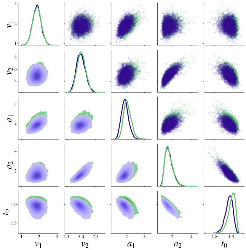
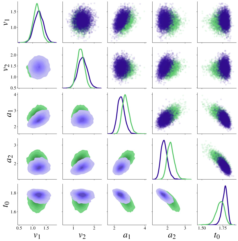
(a) Well-specified: Similar posteriors.

(b) Misspecified: Dissimilar posteriors.

Figure 2: Preview of Experiment 4 on reaction time modeling in psychological experiments (Section 4.4). Posteriors obtained via MCMC (Stan) and simulation-based inference (SBI; BayesFlow) are very similar when the model is well-specified (left). However, a simulation gap (here: not accounting for occasional slow responses due to mind wandering) leads to considerable disagreement between these methods (right).

In this work, we propose a new misspecification measure that can be trained in an unsupervised fashion (i. e., without knowledge of $\mathcal{M}^{*}$ or training data from the true data distribution $p^{*}(\boldsymbol{x})$) and reliably quantifies by how much $\mathcal{M}^{*}$ deviates from $\mathcal{M}$ at test time. Figure 1 illustrates how we achieve this by splitting the task between two neural networks, the summary network $h_{\psi}$ and the inference network $f_{\phi}$. This allows us to measure the misspecification in summary space, where it amounts to a distribution mismatch test that can be elegantly implemented by maximum mean discrepancy (MMD; Gretton et al., 2012).

In principle, we could detect misspecification directly in observation space by measuring the discrepancy between the true distribution $p^{*}(\boldsymbol{x})$ and the model marginal $p(\boldsymbol{x}\,|\,\mathcal{M})$. However, this is a much harder learning problem, because $p^{*}(\boldsymbol{x})$ and $p(\boldsymbol{x}\,|\,\mathcal{M})$ are usually complex high-dimensional distributions. Moreover, $\boldsymbol{x}$ often has variable dimension in practice (e. g., due to a varying number of observations for different subjects or a varying number of time steps in different time series), which further complicates learning in observation space. In contrast, the summary space is designed to have fixed and typically low dimension, and end-to-end training of the two networks ensures that the learned summary statistics are maximally informative about $\boldsymbol{x}$ and follow a simple known distribution (a unit Gaussian) with meaningful MMD scores for misspecification detection. At the same time, summary-based detectors avoid an important shortcoming of traditional Bayesian model checking methods (e.g., Gabry et al., 2019a), which base their diagnostics on the posterior distributions $p(\boldsymbol{\theta}\,|\,\boldsymbol{x},\mathcal{M})$ and therefore become unreliable if these posteriors get distorted in unpredictable ways under model misspecification (cf. 2(b)).

Our experiments clearly demonstrate the power of our new measure both on toy examples with an analytical ground-truth, and on representative scientific tasks in cell biology, cognitive decision making, and disease outbreak dynamics. We show how amortized posterior inference gradually deteriorates as the simulation gap widens and how the proposed misspecification test warns users about suspicious outputs, raises an alarm when predictions are not trustworthy, and guides model designers in their search for better simulators.

In particular, our paper makes the following key contributions:

1. We systematically conceptualize different sources of model misspecification in amortized Bayesian inference with neural networks and propose a new detection criterion that is widely applicable to different model structures, inputs, and outputs.

2. We incorporate this criterion into existing amortized neural posterior estimation methods, both with hand-crafted and learned summary statistics, and extend the associated learning algorithms in a largely non-intrusive manner.

3. We conduct a systematic empirical evaluation of our detection criterion, the influence of the summary space dimension, and the relationship between summary outliers and posterior distortion under various types and strengths of model misspecification.

2 Related Work

Model misspecification has been studied both in the context of standard Bayesian inference and generalizations thereof (i.e., generalized Bayesian inference, see Knoblauch et al., 2019; Schmon et al., 2021). To alleviate model misspecification in generalized Bayesian inference, researchers have investigated probabilistic classifiers (Thomas and Corander, 2019), second-order PAC-Bayes bounds (Masegosa, 2020), scoring rules (Giummolè et al., 2019), priors over a class of predictive models (Loaiza-Maya et al., 2021), or Stein discrepancy as a loss function (Matsubara et al., 2022). Notably, most of these approaches deviate from the standard Bayesian formulation and investigate alternative schemes for belief updating and learning (e.g., replacing the likelihood function with a generic loss function). In contrast, our method remains grounded in the standard Bayesian framework embodying an implicit likelihood principle Berger and Wolpert (1988). Differently, power scaling methods incorporate a modified likelihood (raised to a power $0<\alpha<1)$ in order to prevent potentially overconfident Bayesian updating Grünwald et al. (2017); Holmes and Walker (2017). However, the SBI setting assumes that the likelihood function is not available in closed-form, which makes an explicit modification of the implicitly defined likelihood less obvious.

Neural approaches to amortized SBI can be categorized as either targeting the posterior Radev et al. (2020a); Greenberg et al. (2019), the likelihood Papamakarios et al. (2019); Hermans et al. (2020), or both Wiqvist et al. (2021). These methods employ simulations for training amortized neural approximators which can either generate samples from the posterior directly Radev et al. (2020a); Greenberg et al. (2019); Wiqvist et al. (2021) or in tandem with Markov chain Monte Carlo (MCMC) sampling algorithms Papamakarios et al. (2019); Hermans et al. (2020). Since the behavior of these methods depends on the fidelity of the simulations used as training data, we hypothesize that their estimation quality will be, in general, unpredictable, when faced with atypical real-world data. Indeed, the critical impact of model misspecification in neural SBI has been commonly acknowledged in the scientific research community Cannon et al. (2022); Alquier and Ridgway (2019); Zhang and Gao (2020); Frazier et al. (2020); Frazier and Drovandi (2021); Pacchiardi and Dutta (2022b).

Recent approaches to detect model misspecification in simulation-based inference are usually based on the obtained approximate posterior distribution (e.g., Hermans et al., 2021; Dellaporta et al., 2022; Leclercq, 2022). However, we show in Experiment 1 and Experiment 4 that the approximate posteriors in simulation-based inference tend to show pathological behavior under misspecified models. Posteriors from misspecified models may erroneously look legitimate, rendering diagnostic methods on their basis unreliable. Moreover, the same applies for approaches based on the posterior predictive distribution (Bürkner et al., 2020; Gabry et al., 2019b; Vehtari and Ojanen, 2012) since these also rely on the fidelity of the posterior distribution and can therefore only serve as an indirect measure of misspecification.

A few novel techniques aim to mitigate model misspecification in simulation-based inference to achieve robust inference. Delaunoy et al. (2022) equip neural ratio estimation Hermans et al. (2020) with a balancing condition which tends to produce more conservative posterior approximations. Ward et al. (2022) explore a way to alleviate model misspecification with two neural approximators and subsequent MCMC. While both approaches are appealing in theory, the computational burden of MCMC sampling contradicts the idea of amortized inference and prohibits their use in complex applications with learned summary statistics and large amounts of data. In fact, von Krause et al. (2022) recently used amortized neural SBI on more than a million data sets and demonstrated that an alternative inference method involving non-amortized MCMC would have taken years of sampling per model.

For robust non-amortized ABC samplers, the possibility of utilizing hand-crafted summary statistics as an important element of misspecification analysis has already been explored Frazier et al. (2020); Frazier and Drovandi (2021). Our work parallels these ideas and extends them to the case of learnable summary statistics in amortized SBI on potentially massive data sets, where ABC becomes infeasible. However, we show in Experiment 3 that our method also works with hand-crafted summary statistics. Furthermore, we offer a conceptual discussion on the sources of misspecifications (and their consequences) arising in amortized SBI and explore the connection between posterior errors and model misspecification as a function of the number of summary statistics.

In the field of variational Bayes, recent work has studied the convergence and concentration rates with and without misspecification Alquier and Ridgway (2019); Zhang and Gao (2020). These approaches are not directly transferable to amortized models because the methods used in variational Bayes do not naturally provide a practical “misspecification alarm”, which is needed because neural approximators remain unchanged after the training phase in SBI.

Framing Bayesian model selection as classification Ruff et al. (2018); Pudlo et al. (2016), diverse outlier detection techniques seem viable for uncovering simulation gaps in model comparison settings. Radev et al. (2021a) propose to train regularized evidential networks which learn a higher-order distribution over posterior model probabilities. This way, conclusions about the “absolute misfit” of all models in a set of candidate models can be drawn. However, this approach is not suitable for parameter estimation and currently requires a loss function which does not guarantee a correct approximation of posterior model probabilities.

Finally, from the perspective of deep anomaly detection, our approach for learning informative summary statistics can be viewed as a special case of generic normality feature learning Pang et al. (2022). Standard learned summary statistics are optimized with a generic feature learning objective which is not primarily designed for anomaly detection (Radev et al., 2020a). However, since learned summary statistics are also optimized to be maximally informative for posterior inference, they are forced to capture underlying data regularities Pang et al. (2022). This makes the summary statistics equipped with a tractable latent summary space appropriate targets for misspecification detection.

3 Method

This section defines model misspecification as a mismatch between marginal distributions and explains the building blocks and theoretical implications of our proposed detection method in the context of amortized SBI. To shorten notation throughout the manuscript, we use an abbreviated set notation $\smash{\{\boldsymbol{a}^{(n)}\}\equiv\{\boldsymbol{a}^{(n)}\}_{n=1}^{N}}$, since we use the same lowercase and uppercase letter for referencing a set member and denoting set size respectively (e.g., $n\in\{1,\dots,N\})$.

3.1 Defining Model Misspecification

For the purpose of simulation-based inference, we define a generative model as a triple $\mathcal{M}=\big{(}g(\boldsymbol{\theta},\boldsymbol{\xi}),p(\boldsymbol{\xi}\,|\,\boldsymbol{\theta}),p(\boldsymbol{\theta})\big{)}$. Such a model generates data $\boldsymbol{x}\in\mathcal{X}$ according to the system

$$\boldsymbol{x}=g(\boldsymbol{\theta},\boldsymbol{\xi})\quad\textrm{with}\quad\boldsymbol{\xi}\sim p(\boldsymbol{\xi}\,|\,\boldsymbol{\theta}),\;\boldsymbol{\theta}\sim p(\boldsymbol{\theta}),$$ (1)

where $g$ denotes a (randomized) simulator, $\boldsymbol{\xi}\in\Xi$ is a source of randomness (i. e., noise) with density function $p(\boldsymbol{\xi}\,|\,\boldsymbol{\theta})$, and $p(\boldsymbol{\theta})$ encodes prior knowledge about plausible simulation parameters $\boldsymbol{\theta}\in\Theta$. Intuitively, $\boldsymbol{x}$ represents quantities that we can observe and measure. We use the decorated symbol $\accentset{\text{o}}{\boldsymbol{x}}$ to mark data that was in fact observed in the real world and not merely simulated by the assumed model $\mathcal{M}$. The parameters $\boldsymbol{\theta}$ consist of hidden properties whose role in $g$ we explicitly understand and model, and $\boldsymbol{\xi}$ takes care of nuisance effects that we only treat statistically. The abstract spaces $\mathcal{X},\Xi$, and $\Theta$ denote the domain of possible output data (possible worlds), the scope of noise, and the set of admissible model parameters, respectively. The distinction between hidden properties $\boldsymbol{\theta}$ and noise $\boldsymbol{\xi}$ is not entirely clear-cut, but depends on our modeling goals and may vary across applications. Moreover, our understanding of the world is constantly evolving, and yesterday’s noise might become tomorrow’s signal.

Whenever we employ simulations to investigate some real world phenomenon, a close correspondence between model and reality is necessary. Unacceptably large discrepancies between the two realms are known as a simulation gap, and the corresponding model is said to be misspecified. Model misspecification can arise from any of the three model components in isolation or simultaneously. A few illustrative examples show what can go wrong in practice:

1. Misspecified Simulator. In a model for the hydraulic conductivity of a medium, the spatial composition of the material is essential: A simulator relying on the assumption of homogeneity will wrongly predict the behavior of heterogeneous materials, biasing inference results in complex and arbitrary ways (Schöniger et al., 2015; Nowak and Guthke, 2016).

2. Unexpected Contamination. During an ongoing pandemic, data collection may be severely distorted, for example by noisy measurements, systematic underreporting, and delayed data transfer Dehning et al. (2020), to name just a few. An epidemiological model disregarding these factors in $p(\boldsymbol{\xi}\,|\,\boldsymbol{\theta})$ will produce erroneous inferences about key disease parameters, even if the underlying theory was otherwise a good approximation of the disease dynamics.

3. Misspecified Prior. When the admissible region of the prior $p(\boldsymbol{\theta})$ is specified too large—for example, allows negative mass—physically impossible simulations may arise. On the other hand, when the prior is too narrow, the typical generative set of a model may leave out an important subset of observables or lead to unreasonable uncertainty estimates (e.g., in satellite retrievals; Nguyen et al., 2019).

Our generative model formulation is equivalent to the standard factorization of the Bayesian joint distribution into likelihood and prior, $p(\boldsymbol{\theta},\boldsymbol{x}\,|\,\mathcal{M})=p(\boldsymbol{x}\,|\,\boldsymbol{\theta},\mathcal{M})\,p(\boldsymbol{\theta}\,|\,\mathcal{M})$, where $\mathcal{M}$ expresses the prior knowledge and assumptions embodied in the model. The likelihood is obtained by marginalizing the joint distribution $p(\boldsymbol{\xi},\boldsymbol{x}\,|\,\boldsymbol{\theta},\mathcal{M})$ over all possible values of the nuisance parameters $\boldsymbol{\xi}$, that is, over all possible execution paths of the simulation program, for fixed $\boldsymbol{\theta}$:

$$p(\boldsymbol{x}\,|\,\boldsymbol{\theta},\mathcal{M})=\int_{\Xi}p(\boldsymbol{\xi},\boldsymbol{x}\,|\,\boldsymbol{\theta},\mathcal{M})\,\mathrm{d}\boldsymbol{\xi}.$$ (2)

This integral is typically intractable Cranmer et al. (2020), but we assume that it exists and is non-degenerate, that is, it defines a proper density over the constrained manifold $\left(g(\boldsymbol{\theta},\boldsymbol{\xi}),\boldsymbol{\xi}\right)$.Whenever we model a real-world complex system, we assume an unknown (true) generator $\mathcal{M}^{*}$, which yields an unknown (true) distribution $\accentset{\text{o}}{\boldsymbol{x}}\sim p^{*}(\boldsymbol{x})$ and is available to the data analyst only via a finite realization (i. e., actually observed data $\accentset{\text{o}}{\boldsymbol{x}}$). Then, using the Bayesian formulation, we say that a generative model $\mathcal{M}$ is strictly well-specified if

$$p^{*}(\boldsymbol{x})=p(\boldsymbol{x}\,|\,\mathcal{M})\equiv\int_{\Theta}p(\boldsymbol{x}\,|\,\boldsymbol{\theta},\mathcal{M})\,p(\boldsymbol{\theta}\,|\,\mathcal{M})\,\mathrm{d}\boldsymbol{\theta}$$ (3)

for every $\boldsymbol{x}\in\mathcal{X}$. Conversely, a generative model is misspecified if an observable $\boldsymbol{x}\in\mathcal{X}$ exists for which the above equality is violated.

Note that our definition of model misspecification does not assume the existence of a true parameter vector $\boldsymbol{\theta}^{*}$, as required by some definitions relying on asymptotic guarantees van der Vaart (2000). That is, we do not require that the (conditional) likelihood itself matches the assumed data-generating distribution, which would mean $p^{*}(\boldsymbol{x})=p(\boldsymbol{x}\,|\,\boldsymbol{\theta}^{*},\mathcal{M})$ for some ground-truth $\boldsymbol{\theta}^{*}\in\Theta$. Instead, we focus on the marginal likelihood $p(\boldsymbol{x}\,|\,\mathcal{M})$ which represents the entire prior predictive distribution of a model and does not commit to a single most representative parameter vector Lotfi et al. (2022); Masegosa (2020). In this way, multiple models whose marginal distributions are representative of $p^{*}(\boldsymbol{x})$ can be considered well-specified without any reference to some hypothetical ground-truth $\boldsymbol{\theta}^{*}$, which may not even exist for opaque systems with unknown parameters.

Since models necessarily simplify reality, the above strict criterion for well-specified models in Eq. 3 is often unattainable in practice. We therefore relax the requirement by quantifying a model’s degree of misspecification in terms of the information loss incurred by the following simplification: For an acceptable upper bound $\vartheta$ on the information loss, a model is well-specified if $\mathbb{D}\big{[}p^{*}(\boldsymbol{x})\,||\,p(\boldsymbol{x}\,|\,\mathcal{M})\big{]}<\vartheta$ and misspecified otherwise. The symbol $\mathbb{D}$ denotes a divergence metric quantifying the “distance” between the data distributions implied by reality and by the model (the marginal likelihood). Notably, equality in Eq. 3 implies no information loss by modeling $p^{*}(\boldsymbol{x})$ with $p(\boldsymbol{x}\,|\,\mathcal{M})$ and thus leads to a divergence of zero. A natural choice for $\mathbb{D}$ would be a metric from the family of $\mathcal{F}$-divergences, such as the Kullback-Leibler (KL) divergence. However, since the practical computation of $\mathcal{F}$-divergences requires closed-form densities, and thus $p^{*}(\boldsymbol{x})$ to be analytically tractable, we prefer a probability integral metric, such as the Maximum Mean Discrepancy (MMD; Gretton et al., 2012). Using the kernel trick, the MMD can be expressed as

$$\mathbb{MMD}^{2}\big{[}p^{*}(\boldsymbol{x})\,||\,p(\boldsymbol{x}\,|\,\mathcal{M})\big{]}=\mathbb{E}_{p^{*}(\boldsymbol{x})}\big{[}\kappa(\boldsymbol{x},\boldsymbol{x}^{\prime})\big{]}+\mathbb{E}_{p(\boldsymbol{x}\,|\,\mathcal{M})}\big{[}\kappa(\boldsymbol{x},\boldsymbol{x}^{\prime})\big{]}-2\mathbb{E}_{{\scriptstyle\begin{array}[]{RCL}\boldsymbol{x}}{&\sim&p^{*}(\boldsymbol{x})\\ \boldsymbol{x}^{\prime}&\sim&p(\boldsymbol{x}\,|\,\mathcal{M})\end{array}}}\big{[}\kappa(\boldsymbol{x},\boldsymbol{x}^{\prime})\big{]}.$$ (4)

with any positive definite kernel $\kappa(\cdot,\cdot)$. Crucially, this metric is practically tractable because it can be efficiently estimated via finite samples from $p^{*}(\boldsymbol{x})$ and $p(\boldsymbol{x}\,|\,\mathcal{M})$, and it equals zero if and only if the two densities are equal Gretton et al. (2012).

We use sums of Gaussian kernels with different widths $\sigma_{i}$ as an established and flexible universal kernel Muandet et al. (2017). However, Ardizzone et al. (2018) argue that kernels with heavier tails may improve performance by yielding superior gradients for outliers. Thus, we repeated all experiments with a sum of inverse multiquadratic kernels (as proposed by Tolstikhin et al., 2017), and find that the results are essentially equal.

3.2 Neural Architectures for Amortized Inference

Our proposed method can be applied to any framework that uses summary statistics as an input to an amortized posterior approximator Bürkner et al. (2022). We will exemplarily outline the seamless integration of our method into the BayesFlow Radev et al. (2020a) and the SNPE-C (aka APT; Greenberg et al., 2019) frameworks, but our method should also apply to the broader class of scoring-based minimization Pacchiardi and Dutta (2022a) or adversarial Ramesh et al. (2022) approaches. BayesFlow and SNPE-C, as implemented in the respective software toolkits Tejero-Cantero et al. (2020), use different neural architectures and training regimes to minimize the expected KL divergence between approximate and correct simulation posterior

$$\boldsymbol{\psi}^{*},\boldsymbol{\phi}^{*}=\operatorname*{argmin}_{\boldsymbol{\psi},\boldsymbol{\phi}}\mathbb{E}_{p(\boldsymbol{x}\,|\,\mathcal{M})}\left[\int_{\Theta}p(\boldsymbol{\theta}\,|\,\boldsymbol{x},\mathcal{M})\log\frac{p(\boldsymbol{\theta}\,|\,\boldsymbol{x},\mathcal{M})}{q_{\boldsymbol{\phi}}\big{(}\boldsymbol{\theta}\,|\,h_{\boldsymbol{\psi}}(\boldsymbol{x}),\mathcal{M}\big{)}}\,\mathrm{d}\boldsymbol{\theta}\right],$$ (5)

where the expectation is taken with respect to the prior predictive distribution $p(\boldsymbol{x}\,|\,\mathcal{M})$. This criterion reduces to

$$\boldsymbol{\psi}^{*},\boldsymbol{\phi}^{*}=\operatorname*{argmin}_{\boldsymbol{\psi},\boldsymbol{\phi}}\mathbb{E}_{p(\boldsymbol{\theta},\boldsymbol{x}\,|\,\mathcal{M})}\Big{[}-\log q_{\boldsymbol{\phi}}\big{(}\boldsymbol{\theta}\,|\,h_{\boldsymbol{\psi}}(\boldsymbol{x}),\mathcal{M}\big{)}\Big{]},$$ (6)

since the correct posterior $p(\boldsymbol{\theta}\,|\,\boldsymbol{x},\mathcal{M})$ does not depend on the trainable neural network parameters ($\boldsymbol{\psi}$, $\boldsymbol{\phi}$). The above criterion optimizes a summary (aka embedding or conditioning) network with parameters $\boldsymbol{\psi}$ and an inference network with parameters $\boldsymbol{\phi}$ which jointly amortize a generative model $\mathcal{M}$. The summary network transforms input data $\boldsymbol{x}$ of variable size and structure to a fixed-length representation $\boldsymbol{z}=h_{\boldsymbol{\psi}}(\boldsymbol{x})$. The inference network $f_{\boldsymbol{\phi}}$ generates random draws from an approximate posterior $q_{\boldsymbol{\phi}}$ via a normalizing flow, for instance, realized by a conditional invertible neural network (cINN, Ardizzone et al., 2019) or a conditional masked autoregressive flow (cMAF, Papamakarios et al., 2017). Accordingly, we can compute the exact posterior density via the change of variable formula:

$$q_{\boldsymbol{\phi}}(\boldsymbol{\theta}\,|\,h_{\boldsymbol{\psi}}(\boldsymbol{x}),\mathcal{M})=p\Big{(}f_{\boldsymbol{\phi}}\big{(}\boldsymbol{\theta};h_{\boldsymbol{\psi}}(\boldsymbol{x})\big{)}\Big{)}\left|\det\left(\frac{\partial f_{\boldsymbol{\phi}}(\boldsymbol{\theta};h_{\boldsymbol{\psi}}(\boldsymbol{x}))}{\partial\boldsymbol{\theta}}\right)\right|$$ (7)

We approximate the expectation in Eq. 6 via simulations from the generative model $\mathcal{M}$ and repeat the process until convergence, which enables us to perform fully amortized inference (i.e., the posterior functional can be evaluated for any number of observed data sets $\boldsymbol{x}$). Moreover, this objective is self-consistent and results in correct amortized inference under optimal convergence Greenberg et al. (2019); Radev et al. (2020a). However, simulation-based training (cf. Eq. 5) takes the expectation with respect to the model-implied prior predictive distribution $p(\boldsymbol{x}\,|\,\mathcal{M})$, not necessarily the ”true“ real-world distribution $p^{*}(\boldsymbol{x})$. Thus, optimal convergence does not imply correct amortized inference or faithful prediction in the real world when there is a simulation gap, that is, when the assumed training model $\mathcal{M}$ deviates critically from the unknown true generative model $\mathcal{M}^{*}$.

At this point, we may ask whether the same problem also exists for sequential inference, as realized by multi-round SNPE methods Durkan et al. (2020); Greenberg et al. (2019). Whenever we require inference for a single observation $\accentset{\text{o}}{\boldsymbol{x}}$, we can sequentially transform the prior distribution $p(\boldsymbol{\theta})$ into the posterior $p(\boldsymbol{\theta}\,|\,\accentset{\text{o}}{\boldsymbol{x}},\mathcal{M})$ through a series of simulation-based training rounds (Durkan et al., 2020; Greenberg et al., 2019). Typically, we will use the approximate posterior after a given round as the proposal prior for the next round, resulting in a semi-amortized optimization criterion

$$\boldsymbol{\psi}^{*},\boldsymbol{\phi}^{*}=\operatorname*{argmin}_{\boldsymbol{\psi},\boldsymbol{\phi}}\mathbb{E}_{p(\boldsymbol{x}\,|\,\boldsymbol{\theta},\mathcal{M})\widehat{p}(\boldsymbol{\theta}\,|\,\mathcal{M})}\Big{[}-\log\widehat{q}_{\boldsymbol{\phi}}\big{(}\boldsymbol{\theta}\,|\,h_{\boldsymbol{\psi}}(\boldsymbol{x}),\mathcal{M}\big{)}\Big{]},$$ (8)

where $\widehat{p}(\boldsymbol{\theta}\,|\,\mathcal{M})$ is the current proposal distribution and the approximate posterior $\widehat{q}_{\boldsymbol{\phi}}$ is represented as a categorical distribution over a discrete set of atomic proposals in order to be tractable Greenberg et al. (2019). In this way, the neural approximator specializes for estimating solely the parameters of $\accentset{\text{o}}{\boldsymbol{x}}$, since information from the observed data is used to narrow down the prior $p(\boldsymbol{\theta})$ to the typical set of $p(\boldsymbol{\theta}\,|\,\boldsymbol{x},\mathcal{M})$. Still, the first round in sequential inference depends only on the simulator outputs, so simulation gaps are likely to remain problematic, potentially propagating posterior inference errors through further training rounds. Indeed, we demonstrate this behavior in Experiment 1.

3.3 Structured Summary Statistics

In simulation-based inference, summary statistics have a dual purpose, because (i) they are fixed-length vectors, even if the input data $\boldsymbol{x}$ have variable length; and (ii) they usually contain crucial features of the data, which drastically simplifies neural posterior inference. However, in complex real-world scenarios (such as decision making or COVID-19 modeling, cf. Experiments 4 and 5), it is not feasible to rely on hand-crafted summary statistics. Thus, combining neural posterior inference with learned summary statistics leverages the benefits of summary statistics (i.e., compression to fixed-length vectors) while avoiding the virtually impossible task of designing hand-crafted summary statistics for complex models.

Algorithm 1 Misspecification-aware amortized Bayesian inference. The algorithm illustrates online learning for simplicity. The training phase can utilize any other learning paradigm as well (e.g., round-based). Thus, details like batch size or round indices are omitted in the training phase of the algorithm.

1:Training phase:

2:repeat

3:     Sample parameters and data $(\boldsymbol{\theta},\boldsymbol{x})$ from the specified generative model $\mathcal{M}$.

4:     Pass the data $\boldsymbol{x}$ through the summary network: $\boldsymbol{z}=h_{\boldsymbol{\psi}}(\boldsymbol{x})$.

5:     Compute $-\log q_{\boldsymbol{\phi}}\big{(}\boldsymbol{\theta}\,|\,\boldsymbol{z},\mathcal{M}\big{)}$ using Eq. 7.

6:     Compute Monte Carlo estimate of Eq. 9 as a loss function.

7:     Update neural network parameters $\boldsymbol{\psi},\boldsymbol{\phi}$ via backpropagation.

8:until convergence to $\widehat{\boldsymbol{\psi}},\widehat{\boldsymbol{\phi}}$

9:

10:Inference phase (given $N$ observed or test data sets $\{\accentset{\text{o}}{\boldsymbol{x}}^{(n)}\}$, query $L$ draws from the amortized posterior, use $M$ draws from the validation summary distribution):

11:for $m=1,\ldots,M$ do

12:     Re-use data set $\boldsymbol{x}^{(m)}$ from the training phase or simulate a new one from $\mathcal{M}$.

13:     Pass the data set $\boldsymbol{x}^{(m)}$ through the converged summary network: $\boldsymbol{z}^{(m)}=h_{\widehat{\boldsymbol{\psi}}}(\boldsymbol{x}^{(m)})$.

14:end for

15:for $n=1,\ldots,N$ do

16:     Pass the observed data set $\accentset{\text{o}}{\boldsymbol{x}}^{(n)}$ through the summary network: $\accentset{\text{o}}{\boldsymbol{z}}^{(n)}=h_{\widehat{\boldsymbol{\psi}}}(\accentset{\text{o}}{\boldsymbol{x}}^{(n)})$.

17:     Pass $\accentset{\text{o}}{\boldsymbol{z}}^{(n)}$ through the posterior approximator for $L$ draws $\{\boldsymbol{\theta}^{(n,l)}\}$ from $q_{\widehat{\boldsymbol{\phi}}}(\boldsymbol{\theta}\,|\,\accentset{\text{o}}{\boldsymbol{z}}^{(n)})$

18:end for

19:Estimate the MMD distance of the inference data $\{\accentset{\text{o}}{\boldsymbol{z}}^{(n)}\}$ from the validation summary space under the generative model $\mathcal{M}$ from training: $\widehat{\mathrm{MMD}}^{2}\left(\left\{\accentset{\text{o}}{\boldsymbol{z}}^{(n)}\right\}\,||\,\left\{\boldsymbol{z}^{(m)}\right\}\right)$.

20:return Draws from the approximate posterior distribution for each queried data set $\accentset{\text{o}}{\boldsymbol{x}}^{(n)}$ $\{\boldsymbol{\theta}^{(n,l)}\}$ and $\widehat{\mathrm{MMD}}^{2}\left(\left\{\accentset{\text{o}}{\boldsymbol{z}}^{(n)}\right\}\,||\,\left\{\boldsymbol{z}^{(m)}\right\}\right)$.

In simulation-based inference, the summary network $h_{\boldsymbol{\psi}}$ acts as an interface between the data $\boldsymbol{x}$ and the inference network $f_{\boldsymbol{\phi}}$. Its role is to learn maximally informative summary vectors of fixed size $S$ from complex and structured observations (e. g., sets of $i.\-i.\-d.\-$ measurements or multivariate time series). Since the learned summary statistics are optimized to be maximally informative for posterior inference, they are forced to capture underlying data regularities (cf. Section 2). Therefore, we deem the summary network’s representation $\boldsymbol{z}=h_{\boldsymbol{\psi}}(\boldsymbol{x})$ as an adequate target to detect simulation gaps.

Specifically, we propose to prescribe an $S$-dimensional multivariate unit Gaussian distribution to the summary space, $p\big{(}\boldsymbol{z}=h_{\boldsymbol{\psi}}(\boldsymbol{x})\,|\,\mathcal{M}\big{)}\approx\mathcal{N}(\boldsymbol{z}\,|\,\boldsymbol{0},\mathbb{I})$, by minimizing the MMD between summary network outputs and random draws from a unit Gaussian distribution. To ensure that the summary vectors comply with the support of the Gaussian density, we use a linear (bottleneck) output layer with $S$ units in the summary network. Thus, a random vector in summary space takes the form $h_{\boldsymbol{\psi}}(\boldsymbol{x})\equiv\boldsymbol{z}\equiv(z_{1},\ldots,z_{S})\in\mathbb{R}^{S}$. The extended optimization objective then becomes

$$\boldsymbol{\psi}^{*},\boldsymbol{\phi}^{*}=\operatorname*{argmin}_{\boldsymbol{\psi},\boldsymbol{\phi}}\mathbb{E}_{p(\boldsymbol{\theta},\boldsymbol{x}\,|\,\mathcal{M})}\Big{[}-\log q_{\boldsymbol{\phi}}\big{(}\boldsymbol{\theta}\,|\,h_{\boldsymbol{\psi}}(\boldsymbol{x}),\mathcal{M}\big{)}\Big{]}+\gamma\,\mathbb{MMD}^{2}\big{[}p\big{(}h_{\boldsymbol{\psi}}(\boldsymbol{x})\,|\,\mathcal{M}\big{)}\,||\,\mathcal{N}\big{(}\boldsymbol{0},\mathbb{I}\big{)}\big{]}$$ (9)

with a hyperparameter $\gamma$ to control the relative weight of the MMD term. Intuitively, this objective encourages the approximate posterior $q_{\boldsymbol{\phi}}\big{(}\boldsymbol{\theta}\,|\,h_{\boldsymbol{\psi}}(\boldsymbol{x}),\mathcal{M}\big{)}$ to match the correct posterior and the summary distribution $\smash{p\big{(}h_{\boldsymbol{\psi}}(\boldsymbol{x})\,|\,\mathcal{M}\big{)}}$ to match a unit Gaussian. The extended objective does not constitute a trade-off between the two terms, since the MMD term merely reshapes the summary distribution in an information preserving manner. Indeed, our experiments confirm that the extended objective does not impose restrictions on learnable posteriors or other limits on amortized simulation-based inference.

It is worth noting that this method is also directly applicable to hand-crafted summary statistics. Hand-crafted summary statistics already have fixed length and usually contain rich information for posterior inference. Thus, the task of the summary network $h_{\psi}$ simplifies to transforming the hand-crafted summary statistics to a unit Gaussian (Eq. 9) to enable model misspecification via distribution matching during test time (see below). We apply our method to hand-crafted summary statistics in Experiment 3.

3.4 Theoretical Implications

Attaining the global minimum of Eq. 9 with an arbitrarily expressive neural architecture $\{h_{\boldsymbol{\psi}^{*}},f_{\boldsymbol{\phi}^{*}},\mathcal{M}\}$ implies that (i) the inference and summary network jointly amortize the analytic posterior $p(\boldsymbol{\theta}\,|\,\boldsymbol{x},\mathcal{M})$; and (ii) the summary network transforms the data $p(\boldsymbol{x}\,|\,\mathcal{M})$ into a unit Gaussian in summary space: $p\big{(}\boldsymbol{z}=h_{\boldsymbol{\psi}^{*}}(\boldsymbol{x})\big{)}=\mathcal{N}(\boldsymbol{z}\,|\,\mathbf{0},\mathbb{I})$. According to (i), the set of inference network parameters $\boldsymbol{\phi}^{*}$ is a minimizer of the (expected) negative log posterior learned by the inference network,

$$\boldsymbol{\phi}^{*}=\operatorname*{argmin}_{\boldsymbol{\phi}}\mathbb{E}_{p(\boldsymbol{z})}\mathbb{E}_{p(\boldsymbol{\theta}\,|\,\boldsymbol{z})}\Big{[}-\log q_{\boldsymbol{\phi}}\big{(}\boldsymbol{\theta}\,|\,\boldsymbol{z}\big{)}\Big{]}.$$ (10)

At the same time, (ii) ensures that deviances in the summary space (according to MMD) imply differences in the data generating processes,

$$\underbrace{\mathbb{MMD}^{2}\big{[}p^{*}(\boldsymbol{z})\,||\,p(\boldsymbol{z}\,|\,\mathcal{M})\big{]}>0}_{\text{summary space difference}}\implies\underbrace{\mathbb{MMD}^{2}\big{[}p^{*}(\boldsymbol{x})\,||\,p(\boldsymbol{x}\,|\,\mathcal{M})\big{]}>0}_{\text{data space difference}},$$ (11)

since a deviation of $p^{*}(\boldsymbol{z}=h_{\boldsymbol{\psi}^{*}}(\boldsymbol{x}))$ from a unit Gaussian means that the summary network is no longer transforming samples from $p(\boldsymbol{x}\,|\,\mathcal{M})$.

Accordingly, the LHS of Eq. 11 no longer guarantees that the inference network parameters $\boldsymbol{\phi}^{*}$ are maximally informative for posterior inference. The preceding argumentation also motivates our augmented objective, since a divergence of summary statistics for observed data $\accentset{\text{o}}{\boldsymbol{z}}=h_{\boldsymbol{\psi}}(\accentset{\text{o}}{\boldsymbol{x}})$ from a unit Gaussian signalizes a deficiency in the assumed generative model $\mathcal{M}$ and a need to revise the latter. We also hypothesize and show empirically that we can successfully detect simulation gaps in practice even when the summary network outputs have not exactly converged to a unit Gaussian (e. g., in the presence of correlations in summary space, cf. Experiment 4 and Experiment 5).

However, the converse of Eq. 11 is not true in general. In other words, a discrepancy in data space (non-zero MMD on the RHS of Eq. 11) does not generally imply a difference in summary space (non-zero MMD on the LHS of Eq. 11). To illustrate this via a counter-example, consider the assumed Gaussian generative model $\mathcal{M}$ defined by

$$\mu \sim p(\mu),$$ (12)

$$x_{1},x_{2} \sim\mathcal{N}(\mu,\sigma^{2}=2),$$

for $N=2$ observations and a summary network with a single-output ($S=1$). Since the variance is fixed, the only inference target is the mean $\mu$.

Then, an optimal summary network $\boldsymbol{\psi}^{*}$ outputs the minimal sufficient summary statistic for recovering the mean, namely the empirical average: $h_{\boldsymbol{\psi}^{*}}(x_{1},x_{2})=\bar{x}\equiv(x_{1}+x_{2})/2$. Consequently, the distribution in summary space is given as $p(\bar{x})=\mathcal{N}(0,1)$. In terms of the MMD criterion, we see that $\mathbb{MMD}^{2}\big{[}\underbrace{p(h_{\boldsymbol{\psi}^{*}}(x_{1},x_{2}))}_{=\mathcal{N}(0,1)}\,||\,\mathcal{N}(0,1)\big{]}=0$.

Now, suppose that the real data are actually generated by a different model $\mathcal{M}^{*}$ with $\accentset{\text{o}}{x}\sim p^{*}(\boldsymbol{x})$ given by

$$\mu \sim p(\mu),$$ (13)

$$\accentset{\text{o}}{x}_{1} \sim\mathcal{N}(\mu,\sigma^{2}=1),$$

$$\accentset{\text{o}}{x}_{2} \sim\mathcal{N}(\mu,\sigma^{2}=3).$$

Clearly, this process $p^{*}(\boldsymbol{x})$ differs from $p(\boldsymbol{x}\,|\,\mathcal{M})$ (Eq. 12) on the data domain according to the MMD metric: $\mathbb{MMD}^{2}\big{[}p^{*}(\boldsymbol{x})\,||\,p(\boldsymbol{x}\,|\,\mathcal{M})\big{]}>0$. However, using the same calculations as above, we find that the summary space for the process $p^{*}(\boldsymbol{x})$ also follows a unit Normal distribution: $p^{*}(\bar{x})=\mathcal{N}(0,1)$. Thus, the processes $p^{*}(\boldsymbol{x})$ and $p(\boldsymbol{x}\,|\,\mathcal{M})$ are indistinguishable in the summary space despite the fact that the first generative model $\mathcal{M}$ is clearly misspecified.

The above example shows that learning minimal sufficient summary statistics for solving the inference task (i.e., the mean in this example) might not be optimal for detecting simulation gaps. In fact, increasing the output dimensions $S$ of the summary network $h_{\boldsymbol{\psi}}$ would enable the network to learn structurally richer (overcomplete) sufficient summary statistics. The latter would be invariant to fewer misspecifications and thus more useful for uncovering simulation gaps. In the above example, an overcomplete summary network with $S=2$ which simply copies and scales the two variables by their corresponding variances is able to detect the misspecification. Experiment 1 studies the influence of the number of summary statistics in a controlled setting and provides empirical illustrations. Experiments 4 and 5 further address the choice of the number of summary statistics in more complex models of decision making and disease outbreak. Next, we describe how to practically detect simulation gaps during inference using only finite realizations from $\mathcal{M}$ and $\mathcal{M}^{*}$.

3.5 Detecting Model Misspecification with Finite Data

Once the simulation-based training phase is completed, we can generate $M$ validation samples $\smash{\{\boldsymbol{\theta}^{(m)},\boldsymbol{x}^{(m)}\}}$ of from our generative model $\mathcal{M}$ and pass them through the summary network to obtain a sample of latent summary vectors $\smash{\{\boldsymbol{z}^{(m)}\}}$, where $\smash{\boldsymbol{z}=h_{\boldsymbol{\psi}}(\boldsymbol{x})}$ denotes the output of the summary network. The properties of this sample contain important convergence information: If $\smash{\boldsymbol{z}}$ is approximately unit Gaussian, we can assume a structured summary space given the training model $\mathcal{M}$. This enables model misspecification diagnostics via distribution checking during inference on real data (see Algorithm 1).

Let $\smash{\{\accentset{\text{o}}{\boldsymbol{x}}^{(n)}\}}$ be an observed sample, either simulated from a different generative model, or arising from real-world observations with an unknown generator. Before invoking the inference network, we pass this sample through the summary network to obtain the summary statistics for the sample: $\smash{\{\accentset{\text{o}}{\boldsymbol{z}}^{(n)}\}}$. We then compare the validation summary distribution $\{\boldsymbol{z}^{(m)}\}$ with the summary statistics of the observed data $\smash{\{\accentset{\text{o}}{\boldsymbol{z}}^{(n)}\}}$ according to the sample-based MMD estimate $\smash{\widehat{\text{MMD}}^{2}\left(p(\boldsymbol{z})\,||\,p(\accentset{\text{o}}{\boldsymbol{z}})\right)}$ (cf. Gretton et al., 2012). Importantly, we are not limited to pre-determined sizes of simulated or real-world data sets, as the MMD estimator is defined for arbitrary $M$ and $N$. To enhance visibility, the figures in the experimental section will depict the square root $\widehat{\text{rMMD}}(\cdot,\cdot)$ of the originally squared MMD estimate.

Whenever we estimate the MMD from finite data, its estimates vary according to a sampling distribution and we can resort to a frequentist hypothesis test to determine the probability of observed MMD values under well-specified models. Although this sampling distribution under the null hypothesis is unknown, we can estimate it from multiple sets of simulations from the generative model, $\smash{\{\boldsymbol{z}^{(m)}\}}$ and $\smash{\{\accentset{\text{o}}{\boldsymbol{z}}^{(n)}\}}$, with $M$ large and $N$ equal to the number of real data sets. Based on the estimated sampling distribution, we can obtain a critical MMD value for a fixed Type I error probability $(\alpha)$ and compare it to the one estimated with the observed data. In general, a larger $\alpha$ level corresponds to a more conservative modeling approach: A larger type I error implies that more tests reject the null hypothesis, which corresponds to more frequent model misspecification alarms and a higher chance that incorrect models will be recognised. Note that the Type II error probability ($\beta$) of this test will generally be high (i. e., the power of the test will be low) whenever the number of real data sets $N$ is very small. However, we show in Experiment 5 that even as few as $5$ real data sets suffice to achieve $\beta\approx 0$ for a complex model on COVID-19 time series.

3.6 Posterior Inference Errors

Given a generative model $\mathcal{M}$, the analytic posterior under the potentially misspecified model $p(\boldsymbol{\theta}\,|\,\boldsymbol{x},\mathcal{M})$ always exists, even if $\mathcal{M}$ is misspecified for the data $\boldsymbol{x}$. Obtaining a trustworthy approximation of the analytic posterior is the fundamental basis for any follow-up inference (e. g., parameter estimation or model comparison) and must be at least an intermediate goal in real world applications. Assuming optimal convergence under a misspecified model $\mathcal{M}$, the amortized posterior $q_{\boldsymbol{\phi}}\big{(}\boldsymbol{\theta}\,|\,\boldsymbol{z}=h_{\boldsymbol{\psi}}(\boldsymbol{x}),\mathcal{M}\big{)}$ still corresponds to the analytic posterior $p(\boldsymbol{\theta}\,|\,\boldsymbol{x},\mathcal{M})$, as any transformed $\accentset{\text{o}}{\boldsymbol{x}}$ arising from $p^{*}(\boldsymbol{x})$ has non-zero density in the latent Gaussian summary space. Thus, the posterior approximator should still be able to obtain the correct pushforward density under $\mathcal{M}$ for any query $\accentset{\text{o}}{\boldsymbol{x}}$. However, optimal convergence can never be achieved after finite training time, so we need to address its implications for the validity of amortized simulation-based posterior inference in practice.

Given finite training data, the summary and inference networks will mostly see simulations from the typical set $\mathcal{T}(\mathcal{M})\subset\mathcal{X}$ of the generative model $\mathcal{M}$, that is, training instances whose self-information $-\log p(\boldsymbol{x}\,|\,\mathcal{M})$ is close to the entropy $\mathbb{E}\big{[}-\log p(\boldsymbol{x}\,|\,\mathcal{M})\big{]}$. In high dimensional problems, the typical set will comprise a rather small subset of the possible outcome space, determined by a complex interaction between the components of $\mathcal{M}$ (Betancourt, 2017). Accordingly, good convergence in practice may mean that i) only observations from $\mathcal{T}(\mathcal{M})$ actually follow the approximate Gaussian in latent summary space and ii) the inference network has only seen enough training examples in $\mathcal{T}(\mathcal{M})$ to learn accurate posteriors for observables $\boldsymbol{x}\in\mathcal{T}(\mathcal{M})$, but remains inaccurate for well-specified, but rare $\boldsymbol{x}\not\in\mathcal{T}(\mathcal{M})$.

Since atypical or improbable outcomes occur rarely during simulation-based training, they have negligible influence on the loss in Eq. 9. Consequently, posterior approximation errors for observations outside of $\mathcal{T}(\mathcal{M})$ can be large, simply because the networks have not yet converged in these unusual regions, and the highly non-linear mapping of the inference network still deviates considerably from the true solution. Better training methods might resolve this problem in the future, but for now our proposed MMD criterion reliably signals low fidelity posterior estimates by quantifying the “distance from the typical generative set” $\mathcal{T}(\mathcal{M})$ in the structured summary space.

Moreover, we hypothesize and demonstrate empirically in the following experiments that the difference between the correct posterior $p(\boldsymbol{\theta}\,|\,\boldsymbol{x},\mathcal{M})$ and the approximate posterior $q_{\boldsymbol{\phi}}(\boldsymbol{\theta}\,|\,h_{\boldsymbol{\psi}}(\boldsymbol{x}),\mathcal{M})$ for misspecified models increases as a function of MMD, and thus the latter also measures the amount of misspecification. Therefore, our MMD criterion serves a dual purpose in practice: It can uncover potential simulation gaps and, simultaneously, signal errors in posterior estimation of rare (but valid) events.

4 Experiments

In the following, we illustrate our method to detect model misspecification in 5 experiments, namely (i) a 2D Gaussian conjugate model for the mean with various simulation gaps in the prior, simulator, and noise; (ii) a 5D Gaussian model with fully estimated covariance matrix and 20 inference parameters; (iii) a point process model of cancer and stromal cell development with hand-crafted summary statistics; (iv) a cognitive model of decision making with tractable likelihood to allow for a comparison with Stan; and (v) a complex epidemiological model with an application to real-world COVID-19 time series and 192 learned summary statistics.

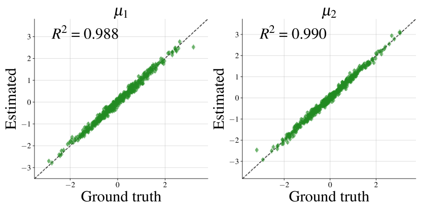
(a) Excellent parameter recovery.

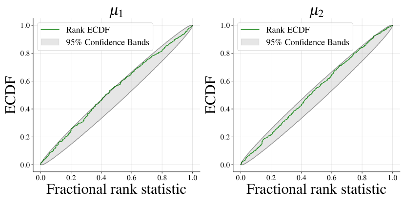
(b) Excellent calibration.

Figure 3: Experiment 1. When the assumed model is well-specified for the observed data ($\mathcal{M}=\mathcal{M}^{*}$), both posterior recovery (3(a)) and calibration (3(b)) remain excellent with our adjusted optimization objective.

4.1 Experiment 1: 2D Gaussian Means

Model (MMS)	Prior	Likelihood
$\mathcal{M}$ (No MMS)	$\boldsymbol{\mu}\sim\mathcal{N}(\boldsymbol{\mu}_{0}=\boldsymbol{0},\boldsymbol{\Sigma}_{0}=\mathbb{I})$	$\boldsymbol{x}_{k}\sim\mathcal{N}(\boldsymbol{\mu},\boldsymbol{\Sigma}=\mathbb{I})$
$\mathcal{M}_{P}$ (Prior)	$\boldsymbol{\mu}\sim\mathcal{N}(\boldsymbol{\mu}_{0}\neq\boldsymbol{0},\boldsymbol{\Sigma}_{0}=\tau_{0}\mathbb{I}),\tau_{0}\in\mathbb{R}^{+}$	$\boldsymbol{x}_{k}\sim\mathcal{N}(\boldsymbol{\mu},\boldsymbol{\Sigma}=\mathbb{I})$
$\mathcal{M}_{S}$ (Simulator)	$\boldsymbol{\mu}\sim\mathcal{N}(\boldsymbol{\mu}_{0}=\boldsymbol{0},\boldsymbol{\Sigma}_{0}=\mathbb{I})$	$\boldsymbol{x}_{k}\sim\mathcal{N}(\boldsymbol{\mu},\boldsymbol{\Sigma}=\tau\mathbb{I}),\tau\in\mathbb{R}^{+}$
$\mathcal{M}_{N}$ (Noise)	$\boldsymbol{\mu}\sim\mathcal{N}(\boldsymbol{\mu}_{0}=\boldsymbol{0},\boldsymbol{\Sigma}_{0}=\mathbb{I})$	$\boldsymbol{x}_{k}\sim\lambda\cdot\mathrm{Beta}(2,5)+(1-\lambda)\cdot\mathcal{N}(\boldsymbol{\mu},\boldsymbol{\Sigma}=\mathbb{I})$

Table 1: Experiment 1. Investigated model misspecifications.

We set the stage by estimating the mean of a $2$-dimensional conjugate Gaussian model with $K=100$ observations per data set and a known analytic posterior in order to illustrate our method. This experiment contains the Gaussian examples from Frazier et al. (2020) and Ward et al. (2022), and extends them by (i) studying misspecifications beyond the likelihood variance (see below); and (ii) implementing continuously widening simulation gaps, as opposed to a single discrete misspecification. The data generating process is defined as

$$\boldsymbol{x}_{k}\sim\mathcal{N}(\boldsymbol{x}\,|\,\boldsymbol{\mu},\boldsymbol{\Sigma})\quad\text{for }k=1,...,K\qquad\text{with }\;\;\boldsymbol{\mu}\sim\mathcal{N}(\boldsymbol{\mu}\,|\,\boldsymbol{\mu}_{0},\boldsymbol{\Sigma}_{0}).$$ (14)

We use a permutation invariant summary network Bloem-Reddy and Teh (2020) with $S=2$ output dimensions, which equal the number of minimal sufficient statistics implied by the analytic posterior. For training the posterior approximator, we set the prior of the generative model $\mathcal{M}$ to a unit Gaussian and the likelihood covariance $\boldsymbol{\Sigma}$ to an identity matrix. The induced misspecifications during test time are outlined in Table 1. We conduct the experiment with BayesFlow and SNPE-C, both equipped with our adjusted optimization objective.

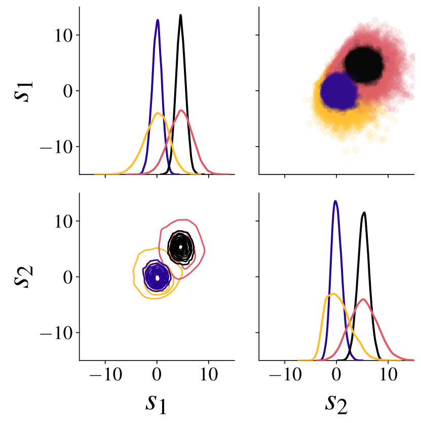
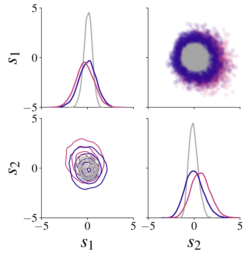
Figure 4: Experiment 1. Summary space samples for the minimal sufficient summary network ($S=2$) from a well-specified model $\mathcal{M}$ (blue) and several misspecified configurations. Left: Prior misspecification can be detected. Right: Noise misspecification can be detected, while simulator scale misspecification is indistinguishable from the validation summary statistics (but see results for $S=4$).

Results. The BayesFlow network trained to minimize the augmented objective (Eq. 9) exhibits excellent recovery of the analytic posterior means when no misspecification is present (see 3(a)). Furthermore, the posterior calibration (SBC; Talts et al., 2020) remains excellent, as shown in 3(b) via simultaneous confidence bands of rank ECDFs Säilynoja et al. (2021). All prior misspecifications manifest themselves in anomalies in the summary space which are directly detectable through visual inspection of the $2$-dimensional summary space in Figure 4 (left). Note that the combined prior misspecification (location and scale) exhibits a summary space pattern that combines the location and scale of the respective location and scale misspecifications. However, based on the $2$-dimensional summary space, misspecifications in the fixed parameters of the likelihood ($\tau$) and mixture noise are not detectable via an increased MMD (see Figure 5, top right).

		Model Misspecification
		Prior ($\mathcal{M}_{P}$)	Simulator ($\mathcal{M}_{S}$) & noise ($\mathcal{M}_{N}$)
Summary Network	minimal
	overcomplete

Figure 5: Experiment 1. Summary space MMD as a function of misspecification severity. White stars indicate the well-specified model configuration (i.e., equal to the training model $\mathcal{M}$).

We further investigate the effect of an overcomplete summary space with respect to the inference task, namely $S=4$ learned summary statistics with an otherwise equal architecture. In addition to prior misspecifications, the overcomplete summary network also captures misspecifications in the noise and simulator via the MMD criterion (see Figure 5, bottom row). Furthermore, the induced misspecifications in the noise and simulator are visually detectable in the summary space samples (see Figure C.1 in the Appendix). Recall that the $2$-dimensional summary space fails to capture these misspecifications (see Figure 5, top right).

		Model Misspecification
		Prior ($\mathcal{M}_{P}$)	Simulator ($\mathcal{M}_{S}$) & noise ($\mathcal{M}_{N}$)
Summary Network	minimal
	overcomplete

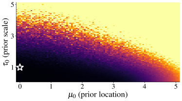
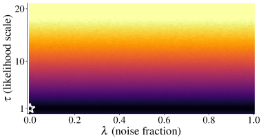
Figure 6: Experiment 1. Posterior Error (RMSE of correct vs. analytic posterior means) as a function of misspecification severity. White stars indicate the well-specified model configuration (i.e., equal to the training model $\mathcal{M}$).

Finally, we compute the error in posterior recovery as a function of the misspecification severity. To ease visualization, we use the RMSE of the approximated posterior mean from $L$ samples $\hat{\overline{\boldsymbol{\theta}}}^{(n)}=\frac{1}{L}\sum_{l=1}^{L}\boldsymbol{\theta}^{(l,n)}$ against the analytic posterior mean $\overline{\boldsymbol{\theta}}^{(n)}$ across a number of $N$ data sets.

Figure 6 illustrates that more severe model misspecifications generally coincide with a larger error in posterior estimation across all model misspecifications for both $S=2$ and $S=4$ learned summary statistics, albeit with fundamental differences, as explained in the following. When processing data emerging from models with misspecified noise and simulator (see Figure 6, right column), minimal and overcomplete summary networks exhibit a drastically different behavior: While the minimal summary network cannot detect noise or simulator simulation gaps, its posterior estimation performance is not heavily impaired either (see Figure 6, top right). On the other hand, the overcomplete summary network is able to capture noise and simulator misspecifications, but also incurs larger posterior inference error (see Figure 6, bottom right). This might suggest a trade-off between model misspecification detection and posterior inference error, depending on the number of learnable summary statistics.

From a practical modeling perspective, researchers might wonder how to choose the number of learnable summary statistics. While an intuitive heuristic might suggest “the more, the merrier”, the observed results in this experiment beg to differ depending on the modeling goals. If the focus in a critical application lies in detecting potential simulation gaps, it might be advantageous to utilize a large (overcomplete) summary vector. However, modelers might also desire a network which is as robust as possible during test time, opting for a smaller number of summary statistics. Experiments 5 addresses this question for a complex non-linear time series model where the number of sufficient summary statistics is unknown.

SNPE-C (APT). Our method successfully detects model misspecification using SNPE-C Greenberg et al. (2019) with the proposed MMD criterion and a structured summary space (see Appendix D). The results are largely equivalent to those obtained with BayesFlow Radev et al. (2020a). The nuanced differences are not soundly interpretable due to the architectural differences of the two frameworks.

4.2 Experiment 2: 5D Gaussian Means and Covariance

(a) Prior misspecification.

(b) Simulator and noise misspecification.

Figure 7: Experiment 2. MMD as a function of model misspecification severity in the prior (left) as well as simulator and noise (right). All induced model misspecifications are detectable through an increased MMD. White stars represent the configuration for the well-specified model (i.e., training model $\mathcal{M}$). The deviating pattern in the top-most row of (7(b)) is caused by the infinite variance of the Student $t$ likelihood with $\nu=2$ degrees of freedom: This is an extreme simulation gap with respect to the unit Gaussian model $\mathcal{M}$, and consequently detected as such.

This experiments extends the Gaussian conjugate model to higher dimensions and a more difficult task, i.e., recovering the means and the full covariance matrix of a $5$-dimensional Gaussian. There is a total of $20$ inference parameters—5 means and 15 (co-)variances—meaning that $20$ summary statistics would suffice to solve the inference task. The mean vector $\boldsymbol{\mu}$ and the covariance matrix $\boldsymbol{\Sigma}$ are drawn from a joint prior, namely a normal-inverse-Wishart distribution ($\text{N-}\mathcal{W}^{-1}$; Barnard et al., 2000). The normal-inverse-Wishart prior $\text{N-}\mathcal{W}^{-1}(\boldsymbol{\mu},\boldsymbol{\Sigma}\,|\,\boldsymbol{\mu}_{0},\lambda_{0},\boldsymbol{\Psi}_{0},\nu_{0})$ implies a hierarchical process, and the implementation details are described in Section A.1 in the Appendix. We set the number of summary statistics to $S=40$ to balance the trade-off between posterior error and misspecification detection (see Experiment 1). The model $\mathcal{M}$ used for training the networks as well as the induced model misspecifications (prior, simulator, and noise) are detailed in Table 4 in the Appendix.

Results. The converged posterior approximator can successfully recover the analytic posterior for all inference parameters when no model misspecification is present. Thus, our method does not impede posterior inference when the models are well-specified. Since the summary space comprises $S=40$ dimensions, visual inspection is no longer feasible, and we resort to the proposed MMD criterion. Both induced prior misspecifications—i.e., location and variance—are detectable through an increased MMD (see 7(a)). Model misspecifications via a heavy-tailed simulator—i. e., Student-$t$ with $\nu=2$ degrees of freedom—, as well as Beta noise, are also detectable with our MMD criterion (see 7(b)).

4.3 Experiment 3: Cancer and Stromal Cell Model

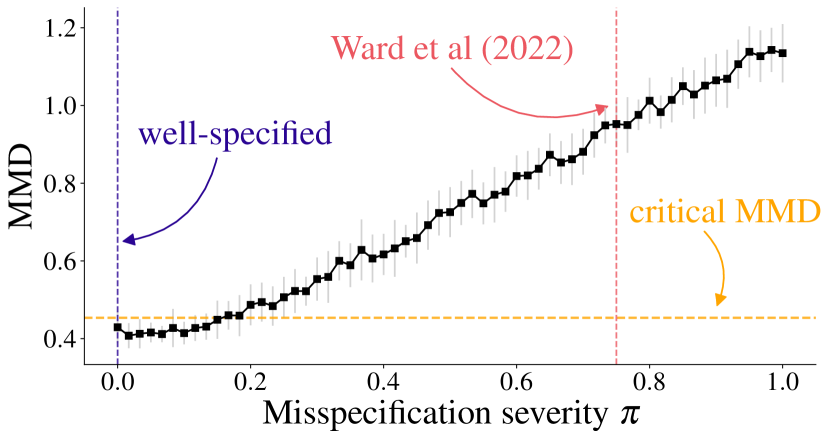
(a) MMD as a function of misspecification severity.

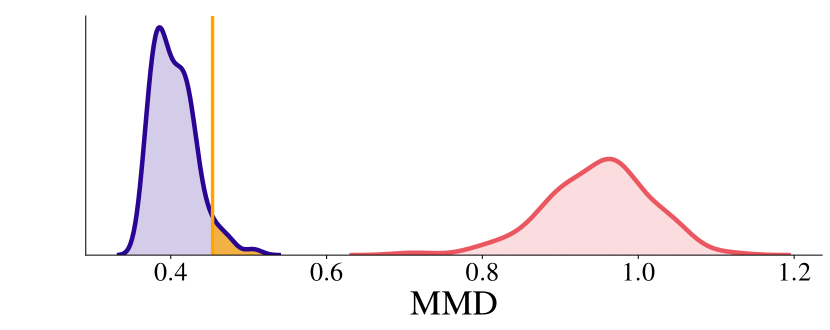
(b) Power for $\pi=0.75$.

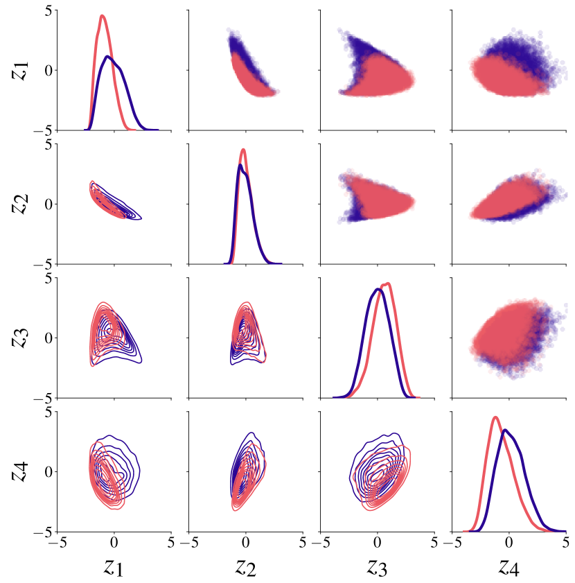
(c) Summary space for $\pi=0.75$.

Figure 8: Experiment 3. MMD increases for rising misspecification severity (8(a); mean and SD of 20 repetitions). The misspecification studied by Ward et al. (2022) is detectable by our hypothesis test (8(b)) and via visual inspection (8(c)). The critical MMD value (orange) in (8(a)) corresponds to the critical MMD in (8(b)).

This experiment illustrates model misspecification detection in a marked point process model of cancer and stromal cells Jones-Todd et al. (2019). We use the original implementation of Ward et al. (2022) with hand-crafted summary statistics and showcase the applicability of our method in scenarios where good summary statistics are known. The inference parameters are three Poisson rates $\lambda_{c},\lambda_{p},\lambda_{d}$, and the setup in Ward et al. (2022) extracts four hand-crafted summary statistics from the 2D plane data: (1–2) number of cancer and stromal cells; (3–4) mean and maximum distance from stromal cells to the nearest cancer cell. All implementation details are described in Section A.2 in the Appendix.

We achieve misspecification during inference by mimicking necrosis, which often occurs in core regions of tumors. A Bernoulli distribution with parameter $\pi$ controls whether a cell is affected by necrosis or not. Consequently, $\pi=0$ implies no necrosis (and thus no simulation gap), and $\pi=1$ entails that all cells are affected. The experiments by Ward et al. (2022) study a single misspecification, namely the case $\pi=0.75$ in our implementation. In order to employ our proposed method for model misspecification detection, we add a small summary network $h_{\boldsymbol{\psi}}:\mathbb{R}^{4}\to\mathbb{R}^{4}$ consisting of three hidden fully connected layers with $64$ units each. This network $h_{\boldsymbol{\psi}}$ merely transforms the hand-crafted summary statistics into a $4$-D unit Gaussian (cf. Algorithm 1).

Results. Our MMD misspecification score increases with increasingly severe model misspecification (i.e., increasing necrosis rate $\pi$), see 8(a). What is more, for the single misspecification $\pi=0.75$ studied by Ward et al. (2022), we illustrate (i) the power of our proposed hypothesis test; and (ii) the summary space distribution for misspecified data. The power ($1-\beta$) essentially equals $1$, as shown in 8(b): The MMD sampling distributions under the training model ($H_{0}$) and under the observed data generating process ($\mathcal{M}^{*}$) are completely separated. In fact, 8(c) unveils that the induced model misspecification is directly visible in the outputs of the summary network $h_{\boldsymbol{\psi}}$.

4.4 Experiment 4: Drift Diffusion Model

(a) MMD as a function of misspecification severity.

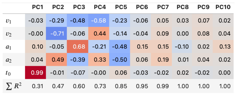
(b) Correlation between parameters $\boldsymbol{\theta}$ and principal components (PCs) of learned summary statistics.

Figure 9: Experiment 4. Contamination of reaction times is detectable with our method (9(a)), and the principal components from the learned summary statistics coincide with the true parameters $\boldsymbol{\theta}$ (9(b)). White star indicates the configuration for the well-specified model (i.e., training model $\mathcal{M}$ without contamination).

This experiment aims to (i) apply the new optimization objective to a complex model of decision making; (ii) illustrate the effect of dimensionality reduction (principal component analysis); (iii) tackle strategies to determine the required number of learned summary statistics in more complex applications; and (iv) compare the posterior estimation of BayesFlow under a misspecified model with the estimation provided by the Stan implementation of HMC-MCMC Carpenter et al. (2017); Stan Development Team (2022) as a current gold-standard for Bayesian inference.

We focus on the drift diffusion model (DDM)—a cognitive model describing reaction times (RTs) in binary decision tasks Ratcliff and McKoon (2008) which is well amenable to amortized inference Radev et al. (2020b). The DDM assumes that perceptual information for a choice alternative accumulates continuously according to a Wiener diffusion process. Thus, the change in information $\mathrm{d}x_{j}$ in experimental condition $j$ follows a random walk with drift and Gaussian noise: $\mathrm{d}x_{j}=v\mathrm{d}t+\xi\sqrt{\mathrm{d}t}$ with $\xi\sim\mathcal{N}(0,1)$. Our model implementation assumes five free parameters $\boldsymbol{\theta}=(v_{1},v_{2},a_{1},a_{2},t_{0})$ which produce $2$-dimensional data stemming from two simulated conditions. The summary network is a permutation-invariant network which reduces $i.\,i.\,d.\$RT data sets to $S=10$ summary statistics each. We realize a simulation gap by simulating typically observed contaminants: fast guesses (e. g., due to inattention), very slow responses (e. g., due to mind wandering), or a combination of the two. The parameter $\lambda$ controls the fraction of the observed data which is contaminated (see Section A.3 in the Appendix for implementation details). For the comparison with Stan, we simulate $100$ uncontaminated DDM data sets and three scenarios (fast guesses, slow responses, fast and slow combined) with a fraction of $\lambda=10\%$ contaminants.

Results. During inference, our criterion reliably detects the induced misspecifications: Increasing fractions $\lambda$ of contaminants (fast, slow, and combined) manifest themselves in increasing MMD values (see 9(a)). The results of applying PCA to the summary network outputs $\{\accentset{\text{o}}{\boldsymbol{z}}^{(n)}\}$ for the well-specified model (no contamination) are illustrated in 9(b). We observe that the first five principal components exhibit a large overlap with the true model parameters $\boldsymbol{\theta}$ and jointly account for 85% of the variance in the summary output. Furthermore, the drift rates and decision thresholds within conditions are entangled (i. e., $v_{1},a_{1}$ and $v_{2},a_{2}$). This entanglement mimics the strong posterior correlations observed between these two parameters. In practical applications, dimensionality reduction might act as a guideline for determining the number of minimally sufficient summary statistics or parameter redundancies for a given problem.

Model (Contamination)	Posterior error MMD	Summary space MMD
$\mathcal{M}_{\ }$: Uncontaminated	$0.25\,[0.13,0.56]$	$0.45\,[0.42,0.52]$
$\mathcal{M}_{1}$: Fast contaminants	$2.66\,[1.44,3.40]$	$2.68\,[2.61,2.74]$
$\mathcal{M}_{2}$: Slow contaminants	$0.55\,[0.23,1.01]$	$1.18\,[1.13,1.26]$
$\mathcal{M}_{3}$: Fast & slow contaminants	$1.90\,[0.83,3.18]$	$2.33\,[2.19,2.43]$

Table 2: Experiment 4. Posterior error of the approximate neural posterior (MMD to Stan samples; median and 95% CI). The bootstrapped MMD values for the summary statistics of the $100$ investigated data sets and $1\,000$ samples from the uncontaminated model $\mathcal{M}$ illustrate that posterior errors are mirrored by anomalies in the summary space and thus detectable.

For the comparison with Stan, we juxtapose $4\,000$ samples from the approximate neural posterior with $4\,000$ samples obtained from the Stan sampler after ensuring MCMC convergence and sufficient sampling efficiency for each data set (see Figure 2 for an illustration). Because Stan is currently considered state-of-the-art for likelihood-based Bayesian inference, we assume the Stan samples are representative of the correct posterior under the potentially misspecified model (see Section 3.6). In order to quantify the difference between the posterior samples from BayesFlow and Stan, we use the MMD criterion as well. When no model misspecification is present, the posterior samples from BayesFlow and Stan match almost perfectly (see 2(a)). This means that our augmented optimization objective still enables correct posterior approximation under well-specified models. In contrast, the results in 2(b) and Table 2 clearly indicate that the amortized posteriors deteriorate as a result of the induced misspecification. Moreover, these results closely mirror the overall detectability of misspecification obtained by matching the summary representations of $1000$ data sets from the uncontaminated process with the representations of the $100$ data sets for each of the above scenarios via MMD (see Table 2).

4.5 Experiment 5: Epidemiological Model for COVID-19

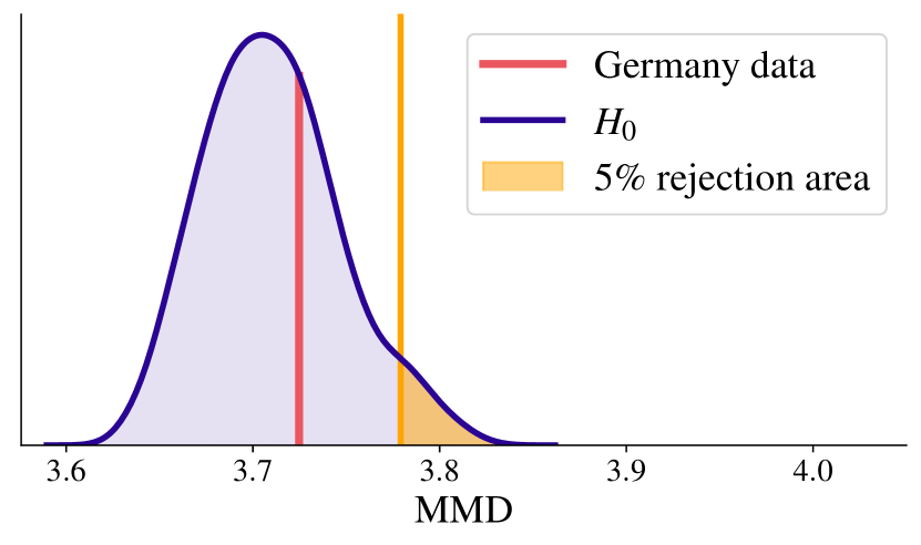
(a) Representation of Germany’s COVID-19 time series with respect to the MMD distribution under the null hypothesis $H_{0}:p^{*}(\boldsymbol{x})=p(\boldsymbol{x}\,|\,\mathcal{M})$.

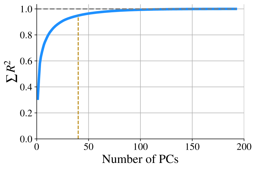
(b) Cumulative explained variance ratio for the summary network output as a function of the number of principal components (PC).

Figure 10: Experiment 5. The observed German COVID-19 time series is well-specified with respect to the training model $\mathcal{M}$ (10(a)), and the first $40$ principal components jointly account for $95\%$ of the variance in the summary network outputs (10(b); golden dashed line).

Compartmental models in epidemiology are very popular for inferring relevant disease parameters, simulating possible outbreak scenarios, and projecting future outcomes Dehning et al. (2020). Given the abundance of such models and their increasing complexity, the importance of detecting simulation gaps for trustworthy inference is two-fold. First, since substantial conclusions are based on the posterior distributions of model parameters, it is important that these distributions are formally correct even when models do not capture all relevant real-world factors. Second, given the dynamic aspect of these models, it is important to detect if an initially well-specified model becomes misspecified at a later time, so the model and its predictions can be amended.

As a final real-world example, we thus focus on a high-dimensional compartmental model representing the early months of the COVID-19 pandemic in Germany Radev et al. (2021b). Here, we investigate the utility of our distribution matching method to detect simulation gaps in a much more realistic and non-trivial extension of the SIR settings in Lueckmann et al. (2021b) and Ward et al. (2022) with substantially increased complexity. Moreover, we perform inference on real COVID-19 data from Germany and use our new method to test whether the model used in Radev et al. (2021b) is misspecified, possibly undermining the trustworthiness of political conclusions that are based on the inferred posteriors. To achieve this, we train a BayesFlow setup identical to Radev et al. (2021b) but using our new optimization objective (Eq. 9) to encourage a structured summary space. We then simulate $1000$ time series from the training model $\mathcal{M}$ and $1000$ time series from three misspecified models: (i) a model $\mathcal{M}_{1}$ without an intervention sub-model; (ii) a model $\mathcal{M}_{2}$ without an observation sub-model; (iii) a model $\mathcal{M}_{3}$ without a latent “carrier” compartment Dehning et al. (2020).

Model	Bootstrap MMD			Power ($1-\beta$)
	$N=1$	$N=2$	$N=5$	$N=1$	$N=2$	$N=5$
$\mathcal{M}_{\ }$	$3.70\,[3.65,3.79]$	$2.61\,[2.54,2.91]$	$1.66\,[1.59,1.84]$	—	—	—
$\mathcal{M}_{1}$	$3.76\,[3.72,3.80]$	$2.86\,[2.62,3.16]$	$2.11\,[1.82,2.50]$	$.998$	$.958$	$\approx 1.0$
$\mathcal{M}_{2}$	$3.80\,[3.73,3.83]$	$2.81\,[2.65,3.00]$	$2.01\,[1.82,2.19]$	$.789$	$.804$	$\approx 1.0$
$\mathcal{M}_{3}$	$3.78\,[3.74,3.83]$	$2.81\,[2.68,3.11]$	$2.07\,[1.92,2.41]$	$.631$	$.690$	$\approx 1.0$

Table 3: Experiment 5. Results for different variations of the COVID-19 compartmental model. We report the median and 95% CI of 100 bootstrap samples.

Results. Table 3 shows the MMD between the summary representation of $N=1,2,5$ bootstrapped time series from each model and the summary representation of the $1000$ time series from model $\mathcal{M}$ (see Section B for bootstrapping details). We also calculate the power ($1-\beta$) of our hypothesis test for each misspecified model under the sampling distribution estimated from $1\,000$ samples of the $1\,000$ time series from $\mathcal{M}$ at a type I error probability of $\alpha=.05$. We observe that the power of the test rapidly increases with more data sets and the Type II error probability ($\beta$) is essentially zero for as few as $N=5$ time series (see Figure 11).

As a next step, we pass the reported COVID-19 data between 1 March and 21 April 2020 (data from Dong et al., 2020, under CC BY 4.0 license) through the summary network and compute the critical MMD value for a sampling-based hypothesis test with an $\alpha$ level of $.05$ (see 10(a)). The MMD of the Germany data is well below the critical MMD value (it essentially lies in the bulk of the distribution), leading to the conclusion that the assumed training model $\mathcal{M}$ is well-specified for this time period. Finally, we perform linear dimensionality reduction (PCA) on the summary space and find that the first 40 principal components jointly explain $95\%$ of the variance in the $192$-dimensional summary space outputs (see 10(b)). Thus, a $40$-dimensional learned summary vector might provide a good approximation of the true (unknown) minimally sufficient summary statistics and render inference less fragile in the face of potential misspecifications (cf. Experiment 1).

	$N=1$	$N=2$	$N=5$
$\mathcal{M}_{1}$
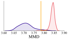
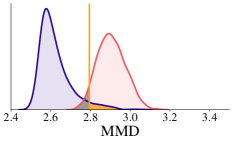
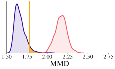
$\mathcal{M}_{2}$
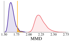
$\mathcal{M}_{3}$

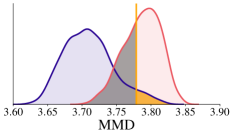
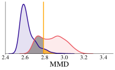
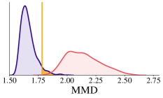
Figure 11: Experiment 5. Detailed illustration of the power analysis. Table 3 contains the test power ($1-\beta$) for each scenario, and as few as $N=5$ observed data sets suffice to achieve a negligible type II error $\beta\approx 0$.

5 Conclusions

With this work, we approached a fundamental problem in amortized simulation-based Bayesian inference, namely, capturing posterior errors due to model misspecification. We argued that misspecified models might cause so-called simulation gaps, resulting in deviations between simulations during training time and actual observed data at test time. We further showed that simulation gaps can be detrimental for the performance and faithfulness of simulation-based inference relying on neural networks. We proposed to increase the networks’ awareness of posterior errors by compressing simulations into a structured latent summary space induced by a modified optimization objective in an unsupervised fashion. We then applied the maximum mean discrepancy (MMD) estimator, equipped with a sampling-based hypothesis test, as a criterion to spotlight discrepancies between model-implied and actually observed distributions in summary space. While we focused on the application to SNPE-C and BayesFlow, the proposed method can be easily integrated into other frameworks with learned or hand-crafted summary statistics as well.

The proposed method can be extended and modified in multiple ways. While we optimized the summary space to follow a spherical Gaussian distribution, our method is likewise applicable to other latent distributions. For example, a heavy-tailed summary distribution (e. g., $\alpha$-stable distributions with tunable tail parameters) would reduce the impact of outliers in latent space. Furthermore, the sampling-based hypothesis test in summary space can be readily replaced with a more sophisticated statistical testing regime for out-of-distribution detection Bergamin et al. (2022). The idea of Frazier et al. (2020) to detect simulation gaps by posterior discrepancies in an ensemble of differently configured approximator instances is interesting, and future work might incorporate this into simulation-based neural inference. In addition, considerations on information geometry and non-Euclidean spaces might guide future research into building more flexible latent spaces and distance metrics Arvanitidis et al. (2021). Our software implementations are openly available at github.com/marvinschmitt/ModelMisspecificationBF and can be seamlessly integrated into an end-to-end workflow for amortized simulation-based inference.

Acknowledgments

This research was supported by the Cyber Valley Research Fund (grant number: CyVy-RF-2021-16), the Deutsche Forschungsgemeinschaft (DFG, German Research Foundation) under Germany’s Excellence Strategy – EXC-2075 - 390740016 (the Stuttgart Cluster of Excellence SimTech) and EXC-2181 - 390900948 (the Heidelberg Cluster of Excellence STRUCTURES), the Deutsche Forschungsgemeinschaft (DFG, German Research Foundation; grant number GRK 2277 “Statistical Modeling in Psychology”), and the Informatics for Life initiative funded by the Klaus Tschira Foundation. The authors gratefully acknowledge the support and funding.

Appendix

Appendix A Implementation Details

A.1 5D Gaussian with Covariance (Experiment 2)

The normal-inverse-Wishart prior $\text{N-}\mathcal{W}^{-1}(\boldsymbol{\mu},\boldsymbol{\Sigma}\,|\,\boldsymbol{\mu}_{0},\lambda_{0},\boldsymbol{\Psi}_{0},\nu_{0})$ implies a hierarchical prior. Suppose the covariance matrix $\boldsymbol{\Sigma}$ has an inverse Wishart distribution $\mathcal{W}^{-1}(\boldsymbol{\Sigma}\,|\,\boldsymbol{\Psi}_{0},\nu_{0})$ and the mean vector $\boldsymbol{\mu}$ has a multivariate normal distribution $\mathcal{N}(\boldsymbol{\mu}\,|\,\boldsymbol{\mu}_{0},\frac{1}{\lambda_{0}}\boldsymbol{\Sigma})$, then the tuple $(\boldsymbol{\mu},\boldsymbol{\Sigma})$ has a normal-inverse-Wishart distribution $\text{N-}\mathcal{W}^{-1}(\boldsymbol{\mu},\boldsymbol{\Sigma}\,|\,\boldsymbol{\mu}_{0},\lambda_{0},\boldsymbol{\Psi}_{0},\nu_{0})$. Finally, the likelihood is Gaussian:$\boldsymbol{x}_{k}\sim\mathcal{N}(\boldsymbol{\mu},\boldsymbol{\Sigma})\;\text{for}\;k=1,\ldots,K$.

For a multivariate Gaussian with unknown mean and unknown covariance matrix, the analytic joint posterior $p(\boldsymbol{\mu}_{p},\boldsymbol{\Sigma}_{p}\,|\,\boldsymbol{x})$ follows a normal-inverse Wishart distribution again:

$$(\boldsymbol{\mu}_{p},\boldsymbol{\Sigma}_{p}\,|\,\boldsymbol{x}) \sim\text{N-}\mathcal{W}^{-1}(\boldsymbol{\mu}_{p},\boldsymbol{\Sigma}_{p}\,|\,\boldsymbol{\mu}_{K},\lambda_{K},\boldsymbol{\Psi}_{K},\nu_{K})\quad\text{with}$$ (15)

$$\boldsymbol{\mu}_{K} =\dfrac{\lambda_{0}\boldsymbol{\mu}_{0}+K\bar{\boldsymbol{x}}}{\lambda_{0}+K},\quad\lambda_{K}=\lambda_{0}+K,\quad\nu_{K}=\nu_{0}+K,$$

$$\boldsymbol{\Psi}_{K} =\boldsymbol{\Psi}_{0}+\sum\limits_{k=1}^{K}(\boldsymbol{x}_{k}-\bar{\boldsymbol{x}})(\boldsymbol{x}_{k}-\bar{\boldsymbol{x}})^{T}+\dfrac{\lambda_{0}K}{\lambda_{0}+K}(\bar{\boldsymbol{x}}-\boldsymbol{\mu}_{0})(\bar{\boldsymbol{x}}-\boldsymbol{\mu}_{0})^{T}$$

The marginal posteriors for $\boldsymbol{\mu}_{p}$ and $\boldsymbol{\Sigma}_{p}$ then follow as Murphy (2007):

$$\boldsymbol{\mu}_{p} \sim t_{\nu_{K}-D-1}\Big{(}\boldsymbol{\mu}_{p}\,\Big{|}\,\boldsymbol{\mu}_{K},\frac{\boldsymbol{\Psi}_{K}^{-1}}{\lambda_{K}(\nu_{K}-D+1)}\Big{)}$$ (16)

$$\boldsymbol{\Sigma}_{p} \sim\mathcal{W}^{-1}(\boldsymbol{\Sigma}_{p}\,|\,\boldsymbol{\Psi}_{K},\nu_{K})$$

The model $\mathcal{M}$ used for training the networks as well as the types of induced model misspecifications are outlined in Table 4.

Model	Prior	Likelihood
$\mathcal{M}$ (No MMS)	$\big{(}\boldsymbol{\mu},\boldsymbol{\Sigma}\big{)}\sim\text{N-}\mathcal{W}^{-1}(\boldsymbol{\mu}_{0}=\boldsymbol{0},\lambda_{0}=5,\boldsymbol{\Psi}=\mathbb{I},\nu=10)$	$\boldsymbol{x}_{k}\sim\mathcal{N}(\boldsymbol{\mu},\boldsymbol{\Sigma})$
$\mathcal{M}_{P}$ (Prior)	$\big{(}\boldsymbol{\mu},\boldsymbol{\Sigma}\big{)}\sim\text{N-}\mathcal{W}^{-1}(\boldsymbol{\mu}_{0}\neq\boldsymbol{0},\lambda_{0}=5,\boldsymbol{\Psi}=\tau_{0}\mathbb{I},\nu=10)$	$\boldsymbol{x}_{k}\sim\mathcal{N}(\boldsymbol{\mu},\boldsymbol{\Sigma})$
$\mathcal{M}_{S}$ (Simulator)	$\big{(}\boldsymbol{\mu},\boldsymbol{\Sigma}\big{)}\sim\text{N-}\mathcal{W}^{-1}(\boldsymbol{\mu}_{0}=\boldsymbol{0},\lambda_{0}=5,\boldsymbol{\Psi}=\mathbb{I},\nu=10)$	$\boldsymbol{x}_{k}\sim t_{\text{df}}(\boldsymbol{\mu},\boldsymbol{\Sigma}),\quad\text{df}\in\mathbb{N}_{>0}$
$\mathcal{M}_{N}$ (Noise)	$\big{(}\boldsymbol{\mu},\boldsymbol{\Sigma}\big{)}\sim\text{N-}\mathcal{W}^{-1}(\boldsymbol{\mu}_{0}=\boldsymbol{0},\lambda_{0}=5,\boldsymbol{\Psi}=\mathbb{I},\nu=10)$	$\boldsymbol{x}_{k}\sim\lambda\cdot\mathrm{Beta}(2,5)+(1-\lambda)\cdot\mathcal{N}(\boldsymbol{\mu},\boldsymbol{\Sigma})$

Table 4: Investigated model misspecifications (MMS) for the $5$-dimensional Gaussian with fully estimated covariance matrix.

In the evaluation, we compare the means of the approximate posterior samples with the first moment of the respective marginal analytic posterior from Eq. 16. We evaluate correlation matrices with standard deviations on the diagonal. For the $t$ distributed posterior mean and inverse-Wishart distributed posterior covariance, we obtain Mardia et al. (1979):

$$\mathbb{E}(\boldsymbol{\mu}_{p})=\boldsymbol{\mu}_{K},\quad\mathbb{E}(\boldsymbol{\Sigma}_{p})=\frac{\boldsymbol{\Psi}_{K}}{\nu_{K}-D-1}$$ (17)

A.2 Cancer and Stromal Cells (Experiment 3)

As implemented by Ward et al. (2022), the CS model simulates the development of cancer and stromal cells. The respective cell counts (total $N_{c}$, unobserved parents $N_{p}$, daughters for each parent $N_{d}^{(i)}$) are stochastically defined through Poisson distributions

$$N_{c}\sim\mathrm{Poisson}(\lambda_{c}),\quad N_{p}\sim\mathrm{Poisson}(\lambda_{c}),\quad N_{d}^{(i)}\sim\mathrm{Poisson}(\lambda_{c}),\quad i=1,\ldots,N_{p}.$$ (18)

The distance based metrics for the hand-crafted summary statistics 3–4 are empirically approximated from 50 stromal cells to avoid computing the full distance matrix Ward et al. (2022). The prior distributions are specified as

$$\lambda_{c}\sim\mathrm{Gamma}(25,0.03),\quad\lambda_{d}\sim\mathrm{Gamma}(5,0.5),\quad\lambda_{p}\sim\mathrm{Gamma}(45,3)$$ (19)

where $\mathrm{Gamma}(a,b)$ denotes the Gamma distribution with location $a$ and rate $b$. To induce model misspecification through necrosis, a Bernoulli variable $w_{i}\sim\mathrm{Bernoulli}(\pi)$ is sampled, removing cancer cells within a specified radius around the parent cell Ward et al. (2022). Thus, the Bernoulli parameter $\pi$ controls the degree of misspecification, ranging from no misspecification ($\pi=0$; no necrosis) to maximal misspecification with respect to that parameter ($\pi=1$; necrosis of all susceptible cells).

A.3 DDM (Experiment 4)

The starting point of the evidence accumulation process is unbiased, $x_{t=0}=\frac{a}{2}$. During training, all parameters are drawn from Gamma prior distributions:

$$v_{1},v_{2},a_{1},a_{2},t_{0}\sim\Gamma(5,0.5).$$ (20)

We first generate uncontaminated data $\boldsymbol{x}^{*}$ from the well-specified generative model $\mathcal{M}$. Second, we randomly choose a fraction $\lambda\in[0,1]$ of the data $\boldsymbol{x}^{*}$. Third, we replace this fraction with data-dependent contaminants $\xi$,

$$\text{Fast guesses:}\quad\xi \sim\mathcal{U}\big{(}0.1,Q_{10}(\boldsymbol{x}^{*})\big{)}$$ (21)

$$\text{Slow responses:}\quad\xi \sim\mathcal{U}\big{(}Q_{75}(\boldsymbol{x}^{*}),10\big{)},$$

where $Q_{k}(\boldsymbol{x}^{*})$ denotes the $k^{\text{th}}$ percentile of $\boldsymbol{x}^{*}$. The asymmetry in percentiles between fast and slow responses arises from the inherent positive skewness of reaction time distributions. The fixed upper limit of slow response contamination is motivated by the maximum number of iterations of the utilized diffusion model simulator. The contamination procedure is executed separately for each condition and response type. If an experiment features both fast and slow contamination, the fraction $\lambda$ is equally split between fast and slow contamination. The uncontaminated data set is generated once and acts as a baseline for all analyses of an experiment, resulting in a baseline MMD of 0 since $\boldsymbol{x}^{*}$ is unaltered if $\lambda=0$.

Appendix B Bootstrapping Procedure

In Experiment 5, we estimate a sampling distribution of the MMD between samples from the specified training model $\mathcal{M}$ with $\boldsymbol{x}\sim p(\boldsymbol{x}\,|\,\mathcal{M}^{*})$ and samples from the (opaque) observed model $\mathcal{M}^{*}$ with $\accentset{\text{o}}{x}\sim p^{*}(\boldsymbol{x})$. Since simulating time series from the compartmental models is time-consuming, we opt for bootstrapping Stine (1989) on $M=1\,000$ pre-simulated time series $\{\boldsymbol{x}^{(m)}\}$ from $\mathcal{M}$ and $N=1\,000$ pre-simulated time series $\{\accentset{\text{o}}{\boldsymbol{x}}^{(n)}\}$ from $\mathcal{M}^{*}$. In each bootstrapping iteration, we draw $M=1\,000$ samples with replacement from $\{\boldsymbol{x}^{(m)}\}$ as well as $N_{B}\in\{1,2,5\}$ samples (with replacement) from $\{\accentset{\text{o}}{\boldsymbol{x}}^{(n)}\}$ and calculate the MMD between the sets of bootstrap samples.

Appendix C 2D Gaussian Means: Overcomplete Summary Statistics

Figure C.1 shows the latent summary space when overcomplete sufficient summary statistics ($S=4$) are used in Experiment 1 to recover the means of a $2$-dimensional Gaussian. Model misspecification with respect to both simulator and noise is detectable through anomalies in the latent summary space. A network with $S=2$ summary statistics and otherwise equivalent architecture could not capture these types of model misspecification.

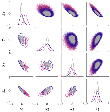
Figure C.1: Pairplot of $10\,000$ latent summary space samples from the overcomplete summary network. Both noise (orange) and simulator (pink) misspecifications are distinguishable from the typical latent generative space (blue).

Appendix D Replication of Experiment 1 with SNPE-C

In the following, we show the results of repeating Experiment 1 with SNPE-C (APT; Greenberg et al., 2019) instead of BayesFlow for posterior inference. The results are largely equivalent to those obtained with the BayesFlow framework.

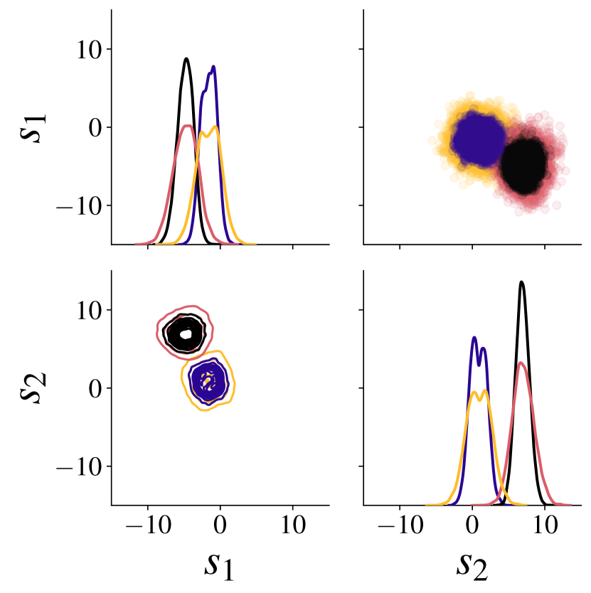
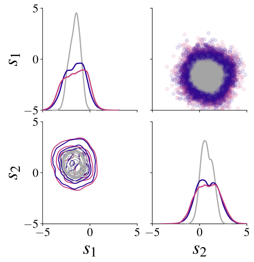
Figure D.1: Experiment 1, SNPE-C. Summary space samples for the minimal sufficient summary network ($S=2$) from a well-specified model $\mathcal{M}$ (blue) and misspecified configurations. Left: Prior misspecification can be detected. Right: Simulator scale misspecification is indistinguishable from the validation summary statistics.

		Model Misspecification
		Prior ($\mathcal{M}_{P}$)	Simulator ($\mathcal{M}_{S}$) & noise ($\mathcal{M}_{N}$)
Summary Network	minimal
	overcomplete

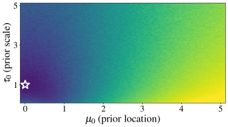
Figure D.2: Experiment 1, SNPE-C. Summary space MMD as a function of misspecification severity. White stars indicate the well-specified model configuration (i.e., equal to the training model $\mathcal{M}$).

References

- Alquier and Ridgway (2019) Pierre Alquier and James Ridgway. Concentration of tempered posteriors and of their variational approximations. arXiv:1706.09293 [cs, math, stat], April 2019. arXiv: 1706.09293.
- Ardizzone et al. (2018) Lynton Ardizzone, Jakob Kruse, Sebastian J. Wirkert, Daniel Rahner, Eric W. Pellegrini, Ralf S. Klessen, Lena Maier-Hein, Carsten Rother, and Ullrich Köthe. Analyzing Inverse Problems with Invertible Neural Networks. CoRR, abs/1808.04730, 2018.
- Ardizzone et al. (2019) Lynton Ardizzone, Carsten Lüth, Jakob Kruse, Carsten Rother, and Ullrich Köthe. Guided Image Generation with Conditional Invertible Neural Networks, 2019.
- Arvanitidis et al. (2021) Georgios Arvanitidis, Miguel González-Duque, Alison Pouplin, Dimitris Kalatzis, and Søren Hauberg. Pulling back information geometry. arXiv preprint arXiv:2106.05367, 2021.
- Barnard et al. (2000) John Barnard, Robert McCulloch, and Xiao-Li Meng. Modelling Covariance Matrices in Terms of Standard Deviations and Correlations, with Application To Shrinkage. Statistica Sinica, 10:1281–1311, 10 2000.
- Bergamin et al. (2022) Federico Bergamin, Pierre-Alexandre Mattei, Jakob D. Havtorn, Hugo Senetaire, Hugo Schmutz, Lars Maaløe, Søren Hauberg, and Jes Frellsen. Model-agnostic out-of-distribution detection using combined statistical tests, March 2022.
- Berger and Wolpert (1988) James O. Berger and Robert L. Wolpert. The likelihood principle. Number v. 6 in Lecture notes-monograph series. Institute of Mathematical Statistics, Hayward, Calif, 2nd ed edition, 1988. ISBN 978-0-940600-13-3.
- Betancourt (2017) Michael Betancourt. A conceptual introduction to Hamiltonian Monte Carlo. arXiv preprint, 2017.
- Bieringer et al. (2021) Sebastian Bieringer, Anja Butter, Theo Heimel, Stefan Höche, Ullrich Köthe, Tilman Plehn, and Stefan T Radev. Measuring QCD Splittings with Invertible Networks. SciPost Physics Proceedings, 10(6), 2021.
- Bloem-Reddy and Teh (2020) Benjamin Bloem-Reddy and Yee Whye Teh. Probabilistic Symmetries and Invariant Neural Networks. J. Mach. Learn. Res., 21:90–1, 2020.
- Bürkner et al. (2022) Paul-Christian Bürkner, Maximilian Scholz, and Stefan Radev. Some models are useful, but how do we know which ones? towards a unified bayesian model taxonomy. arXiv preprint arXiv:2209.02439, 2022.
- Butter et al. (2022) Anja Butter, Tilman Plehn, Steffen Schumann, Simon Badger, Sascha Caron, Kyle Cranmer, Francesco Armando Di Bello, Etienne Dreyer, Stefano Forte, Sanmay Ganguly, et al. Machine learning and lhc event generation. arXiv preprint arXiv:2203.07460, 2022.
- Bürkner et al. (2020) Paul-Christian Bürkner, Jonah Gabry, and Aki Vehtari. Approximate leave-future-out cross-validation for Bayesian time series models. Journal of Statistical Computation and Simulation, 90(14):2499–2523, September 2020. doi: 10.1080/00949655.2020.1783262. arXiv:1902.06281 [stat].
- Cannon et al. (2022) Patrick Cannon, Daniel Ward, and Sebastian M. Schmon. Investigating the Impact of Model Misspecification in Neural Simulation-based Inference, September 2022. arXiv:2209.01845 [cs, stat].
- Carpenter et al. (2017) Bob Carpenter, Andrew Gelman, Matthew D Hoffman, Daniel Lee, Ben Goodrich, Michael Betancourt, Marcus Brubaker, Jiqiang Guo, Peter Li, and Allen Riddell. Stan: A probabilistic programming language. Journal of statistical software, 76(1), 2017.
- Cranmer et al. (2020) Kyle Cranmer, Johann Brehmer, and Gilles Louppe. The frontier of simulation-based inference. Proceedings of the National Academy of Sciences, 117(48):30055–30062, 2020.
- Dehning et al. (2020) Jonas Dehning, Johannes Zierenberg, F Paul Spitzner, Michael Wibral, Joao Pinheiro Neto, Michael Wilczek, and Viola Priesemann. Inferring change points in the spread of COVID-19 reveals the effectiveness of interventions. Science, 369(6500), 2020.
- Delaunoy et al. (2022) Arnaud Delaunoy, Joeri Hermans, François Rozet, Antoine Wehenkel, and Gilles Louppe. Towards Reliable Simulation-Based Inference with Balanced Neural Ratio Estimation, August 2022. arXiv:2208.13624 [cs, stat].
- Dellaporta et al. (2022) Charita Dellaporta, Jeremias Knoblauch, Theodoros Damoulas, and François-Xavier Briol. Robust Bayesian Inference for Simulator-based Models via the MMD Posterior Bootstrap. 2022. doi: 10.48550/ARXIV.2202.04744.
- Dong et al. (2020) Ensheng Dong, Hongru Du, and Lauren Gardner. An interactive web-based dashboard to track COVID-19 in real time. The Lancet Infectious Diseases, 20(5):533–534, May 2020. doi: 10.1016/S1473-3099(20)30120-1.
- Durkan et al. (2020) Conor Durkan, Iain Murray, and George Papamakarios. On contrastive learning for likelihood-free inference. In International Conference on Machine Learning, pages 2771–2781. PMLR, 2020.
- Frazier and Drovandi (2021) David T. Frazier and Christopher Drovandi. Robust Approximate Bayesian Inference With Synthetic Likelihood. Journal of Computational and Graphical Statistics, 30(4):958–976, October 2021. doi: 10.1080/10618600.2021.1875839.
- Frazier et al. (2020) David T. Frazier, Christian P. Robert, and Judith Rousseau. Model misspecification in approximate Bayesian computation: consequences and diagnostics. Journal of the Royal Statistical Society: Series B (Statistical Methodology), 82(2):421–444, April 2020. doi: 10.1111/rssb.12356.
- Gabry et al. (2019a) Jonah Gabry, Daniel Simpson, Aki Vehtari, Michael Betancourt, and Andrew Gelman. Visualization in Bayesian workflow. Journal of the Royal Statistical Society: Series A (Statistics in Society), 182(2):389–402, 2019a.
- Gabry et al. (2019b) Jonah Gabry, Daniel Simpson, Aki Vehtari, Michael Betancourt, and Andrew Gelman. Visualization in Bayesian workflow. Journal of the Royal Statistical Society: Series A (Statistics in Society), 182(2):389–402, 2019b. Publisher: Wiley Online Library.
- Ghaderi-Kangavari et al. (2022) Amin Ghaderi-Kangavari, Jamal Amani Rad, and Michael D. Nunez. A general integrative neurocognitive modeling framework to jointly describe EEG and decision-making on single trials. preprint, PsyArXiv, August 2022.
- Giummolè et al. (2019) Federica Giummolè, Valentina Mameli, Erlis Ruli, and Laura Ventura. Objective bayesian inference with proper scoring rules. Test, 28(3):728–755, 2019.
- Gonçalves et al. (2020) Pedro J Gonçalves, Jan-Matthis Lueckmann, Michael Deistler, Marcel Nonnenmacher, Kaan Öcal, Giacomo Bassetto, Chaitanya Chintaluri, William F Podlaski, Sara A Haddad, Tim P Vogels, et al. Training deep neural density estimators to identify mechanistic models of neural dynamics. Elife, 9:e56261, 2020.
- Greenberg et al. (2019) David Greenberg, Marcel Nonnenmacher, and Jakob Macke. Automatic posterior transformation for likelihood-free inference. In International Conference on Machine Learning, pages 2404–2414. PMLR, 2019.
- Gretton et al. (2012) A Gretton, K. Borgwardt, Malte Rasch, Bernhard Schölkopf, and AJ Smola. A Kernel Two-Sample Test. The Journal of Machine Learning Research, 13:723–773, 03 2012.
- Grünwald et al. (2017) Peter Grünwald, Thijs Van Ommen, et al. Inconsistency of Bayesian inference for misspecified linear models, and a proposal for repairing it. Bayesian Analysis, 12(4):1069–1103, 2017.
- Hermans et al. (2020) Joeri Hermans, Volodimir Begy, and Gilles Louppe. Likelihood-free mcmc with amortized approximate ratio estimators. In International Conference on Machine Learning, pages 4239–4248. PMLR, 2020.
- Hermans et al. (2021) Joeri Hermans, Arnaud Delaunoy, François Rozet, Antoine Wehenkel, and Gilles Louppe. Averting a crisis in simulation-based inference. arXiv preprint arXiv:2110.06581, 2021.
- Holmes and Walker (2017) Chris C Holmes and Stephen G Walker. Assigning a value to a power likelihood in a general bayesian model. Biometrika, 104(2):497–503, 2017.
- Jones-Todd et al. (2019) Charlotte M. Jones-Todd, Peter Caie, Janine B. Illian, Ben C. Stevenson, Anne Savage, David J. Harrison, and James L. Bown. Identifying prognostic structural features in tissue sections of colon cancer patients using point pattern analysis: Point pattern analysis of colon cancer tissue sections. Statistics in Medicine, 38(8):1421–1441, April 2019. doi: 10.1002/sim.8046.
- Knoblauch et al. (2019) Jeremias Knoblauch, Jack Jewson, and Theodoros Damoulas. Generalized variational inference: Three arguments for deriving new posteriors. arXiv preprint arXiv:1904.02063, 2019.
- Leclercq (2022) Florent Leclercq. Simulation-based inference of Bayesian hierarchical models while checking for model misspecification, September 2022. arXiv:2209.11057 [astro-ph, q-bio, stat].
- Loaiza-Maya et al. (2021) Ruben Loaiza-Maya, Gael M Martin, and David T Frazier. Focused bayesian prediction. Journal of Applied Econometrics, 36(5):517–543, 2021.
- Lotfi et al. (2022) Sanae Lotfi, Pavel Izmailov, Gregory Benton, Micah Goldblum, and Andrew Gordon Wilson. Bayesian model selection, the marginal likelihood, and generalization. arXiv preprint arXiv:2202.11678, 2022.
- Lueckmann et al. (2017) Jan-Matthis Lueckmann, Pedro J Goncalves, Giacomo Bassetto, Kaan Öcal, Marcel Nonnenmacher, and Jakob H Macke. Flexible statistical inference for mechanistic models of neural dynamics. Advances in Neural Information Processing Systems, 30, 2017.
- Lueckmann et al. (2021a) Jan-Matthis Lueckmann, Jan Boelts, David Greenberg, Pedro Goncalves, and Jakob Macke. Benchmarking simulation-based inference. In International Conference on Artificial Intelligence and Statistics, pages 343–351. PMLR, 2021a.
- Lueckmann et al. (2021b) Jan-Matthis Lueckmann, Jan Boelts, David Greenberg, Pedro Goncalves, and Jakob Macke. Benchmarking Simulation-Based Inference. In Arindam Banerjee and Kenji Fukumizu, editors, Proceedings of The 24th International Conference on Artificial Intelligence and Statistics, volume 130 of Proceedings of Machine Learning Research, pages 343–351. PMLR, April 2021b.
- Mardia et al. (1979) Kantilal Varichand Mardia, John T. Kent, and John M. Bibby. Multivariate analysis. Probability and mathematical statistics. Acad. Press, London, 1979.
- Masegosa (2020) Andres Masegosa. Learning under model misspecification: Applications to variational and ensemble methods. Advances in Neural Information Processing Systems, 33:5479–5491, 2020.
- Matsubara et al. (2022) Takuo Matsubara, Jeremias Knoblauch, François-Xavier Briol, and Chris J. Oates. Robust Generalised Bayesian Inference for Intractable Likelihoods, January 2022. arXiv:2104.07359 [math, stat].
- Muandet et al. (2017) Krikamol Muandet, Kenji Fukumizu, Bharath Sriperumbudur, and Bernhard Schölkopf. Kernel Mean Embedding of Distributions: A Review and Beyond. Foundations and Trends® in Machine Learning, 10(1-2):1–141, 2017. doi: 10.1561/2200000060.
- Murphy (2007) Kevin Murphy. Conjugate Bayesian analysis of the Gaussian distribution, 11 2007.
- Nguyen et al. (2019) Hai Nguyen, Noel Cressie, and Jonathan Hobbs. Sensitivity of optimal estimation satellite retrievals to misspecification of the prior mean and covariance, with application to oco-2 retrievals. Remote Sensing, 11(23):2770, 2019.
- Nowak and Guthke (2016) Wolfgang Nowak and Anneli Guthke. Entropy-based experimental design for optimal model discrimination in the geosciences. Entropy, 18(11):409–434, 2016.
- Pacchiardi and Dutta (2022a) Lorenzo Pacchiardi and Ritabrata Dutta. Likelihood-free inference with generative neural networks via scoring rule minimization. arXiv preprint arXiv:2205.15784, 2022a.
- Pacchiardi and Dutta (2022b) Lorenzo Pacchiardi and Ritabrata Dutta. Score Matched Neural Exponential Families for Likelihood-Free Inference, January 2022b. arXiv:2012.10903 [stat].
- Pang et al. (2022) Guansong Pang, Chunhua Shen, Longbing Cao, and Anton van den Hengel. Deep Learning for Anomaly Detection: A Review. ACM Computing Surveys, 54(2):1–38, March 2022. doi: 10.1145/3439950. arXiv:2007.02500 [cs, stat].
- Papamakarios and Murray (2016) George Papamakarios and Iain Murray. Fast -free inference of simulation models with bayesian conditional density estimation. Advances in neural information processing systems, 29, 2016.
- Papamakarios et al. (2017) George Papamakarios, Theo Pavlakou, and Iain Murray. Masked autoregressive flow for density estimation. Advances in neural information processing systems, 30, 2017.
- Papamakarios et al. (2019) George Papamakarios, David Sterratt, and Iain Murray. Sequential neural likelihood: Fast likelihood-free inference with autoregressive flows. In The 22nd International Conference on Artificial Intelligence and Statistics, pages 837–848. PMLR, 2019.
- Pudlo et al. (2016) Pierre Pudlo, Jean-Michel Marin, Arnaud Estoup, Jean-Marie Cornuet, Mathieu Gautier, and Christian P Robert. Reliable abc model choice via random forests. Bioinformatics, 32(6):859–866, 2016.
- Radev et al. (2020a) Stefan T Radev, Ulf K Mertens, Andreas Voss, Lynton Ardizzone, and Ullrich Köthe. BayesFlow: Learning complex stochastic models with invertible neural networks. IEEE Transactions on Neural Networks and Learning Systems, 2020a.
- Radev et al. (2020b) Stefan T. Radev, Andreas Voss, Eva Marie Wieschen, and Paul-Christian Buerkner. Amortized Bayesian Inference for Models of Cognition, 2020b.
- Radev et al. (2021a) Stefan T Radev, Marco D’Alessandro, Ulf K Mertens, Andreas Voss, Ullrich Köthe, and Paul-Christian Bürkner. Amortized bayesian model comparison with evidential deep learning. IEEE Transactions on Neural Networks and Learning Systems, 2021a.
- Radev et al. (2021b) Stefan T Radev, Frederik Graw, Simiao Chen, Nico T Mutters, Vanessa M Eichel, Till Bärnighausen, and Ullrich Köthe. OutbreakFlow: Model-based Bayesian inference of disease outbreak dynamics with invertible neural networks and its application to the COVID-19 pandemics in Germany. PLOS Computational Biology, 17(10):e1009472, 2021b.
- Ramesh et al. (2022) Poornima Ramesh, Jan-Matthis Lueckmann, Jan Boelts, Álvaro Tejero-Cantero, David S Greenberg, Pedro J Gonçalves, and Jakob H Macke. Gatsbi: Generative adversarial training for simulation-based inference. arXiv preprint arXiv:2203.06481, 2022.
- Ratcliff and McKoon (2008) Roger Ratcliff and Gail McKoon. The Diffusion Decision Model: Theory and Data for Two-Choice Decision Tasks. Neural Computation, 20(4):873–922, April 2008. doi: 10.1162/neco.2008.12-06-420.
- Ruff et al. (2018) Lukas Ruff, Robert Vandermeulen, Nico Goernitz, Lucas Deecke, Shoaib Ahmed Siddiqui, Alexander Binder, Emmanuel Müller, and Marius Kloft. Deep One-Class Classification. In Jennifer Dy and Andreas Krause, editors, Proceedings of the 35th International Conference on Machine Learning, volume 80 of Proceedings of Machine Learning Research, pages 4393–4402. PMLR, July 2018.
- Schmon et al. (2021) Sebastian M. Schmon, Patrick W. Cannon, and Jeremias Knoblauch. Generalized Posteriors in Approximate Bayesian Computation, February 2021. arXiv:2011.08644 [stat].
- Schöniger et al. (2015) Anneli Schöniger, Walter A Illman, Thomas Wöhling, and Wolfgang Nowak. Finding the right balance between groundwater model complexity and experimental effort via Bayesian model selection. Journal of Hydrology, 531:96–110, 2015.
- Shiono (2021) Takashi Shiono. Estimation of agent-based models using Bayesian deep learning approach of BayesFlow. Journal of Economic Dynamics and Control, 125:104082, 2021.
- Stan Development Team (2022) Stan Development Team. The Stan Core Library, 2022. Version 2.30.0.
- Stine (1989) Robert Stine. An Introduction to Bootstrap Methods. Sociological Methods & Research, 18(2-3):243–291, November 1989. doi: 10.1177/0049124189018002003.
- Säilynoja et al. (2021) Teemu Säilynoja, Paul-Christian Bürkner, and Aki Vehtari. Graphical Test for Discrete Uniformity and its Applications in Goodness of Fit Evaluation and Multiple Sample Comparison, November 2021. arXiv:2103.10522 [stat].
- Talts et al. (2020) Sean Talts, Michael Betancourt, Daniel Simpson, Aki Vehtari, and Andrew Gelman. Validating Bayesian Inference Algorithms with Simulation-Based Calibration, October 2020. arXiv:1804.06788 [stat].
- Tejero-Cantero et al. (2020) Alvaro Tejero-Cantero, Jan Boelts, Michael Deistler, Jan-Matthis Lueckmann, Conor Durkan, Pedro J Gonçalves, David S Greenberg, and Jakob H Macke. Sbi–a toolkit for simulation-based inference. arXiv preprint arXiv:2007.09114, 2020.
- Thomas and Corander (2019) Owen Thomas and Jukka Corander. Diagnosing model misspecification and performing generalized Bayes’ updates via probabilistic classifiers. arXiv preprint arXiv:1912.05810, 2019.
- Tolstikhin et al. (2017) Ilya Tolstikhin, Olivier Bousquet, Sylvain Gelly, and Bernhard Schoelkopf. Wasserstein auto-encoders, 2017.
- van der Vaart (2000) Aad W van der Vaart. Asymptotic statistics, volume 3. Cambridge university press, 2000.
- Vehtari and Ojanen (2012) Aki Vehtari and Janne Ojanen. A survey of Bayesian predictive methods for model assessment, selection and comparison. Statistics Surveys, 6(none), January 2012. doi: 10.1214/12-SS102.
- von Krause et al. (2022) Mischa von Krause, Stefan T. Radev, and Andreas Voss. Mental speed is high until age 60 as revealed by analysis of over a million participants. Nature Human Behaviour, 6(5):700–708, May 2022. doi: 10.1038/s41562-021-01282-7.
- Ward et al. (2022) Daniel Ward, Patrick Cannon, Mark Beaumont, Matteo Fasiolo, and Sebastian M. Schmon. Robust Neural Posterior Estimation and Statistical Model Criticism, October 2022. arXiv:2210.06564 [cs, stat].
- Wiqvist et al. (2021) Samuel Wiqvist, Jes Frellsen, and Umberto Picchini. Sequential Neural Posterior and Likelihood Approximation. arXiv preprint arXiv:2102.06522, 2021.
- Zhang and Gao (2020) Fengshuo Zhang and Chao Gao. Convergence rates of variational posterior distributions. The Annals of Statistics, 48(4), August 2020. doi: 10.1214/19-AOS1883.