Geometric continuous-stage exponential energy-preserving integrators for charged-particle dynamics in a magnetic field from normal to strong regimes

Abstract

This paper is concerned with geometric exponential energy-preserving integrators for solving charged-particle dynamics in a magnetic field from normal to strong regimes. We firstly formulate the scheme of the methods for the system in a uniform magnetic field by using the idea of continuous-stage methods, and then discuss its energy-preserving property. Moreover, symmetric conditions and order conditions are analysed. Based on those conditions, we propose two practical symmetric continuous-stage exponential energy-preserving integrators of order up to four. Then we extend the obtained methods to the system in a nonuniform magnetic field and derive their properties including the symmetry, convergence and energy conservation. Numerical experiments demonstrate the efficiency of the proposed methods in comparison with some existing schemes in the literature.

Mathematics Subject Classification (2010): 65P10, 65L05

1 Introduction

The dynamics of charged particles under the influence of external electromagnetic field are of paramount importance in plasma physics and they have important applications [1, 2, 5, 24, 32]. For example, these equations appear in Vlasov equations [8, 9, 10, 11, 12, 27, 31] which are of fundamental importance in tokamak plasmas. This article is concerned with the numerical solution of the following charged-particle dynamics (CPD) (see [16, 18, 40])

$$\begin{array}[c]{ll}\ddot{x}(t)=\dot{x}(t)\times\frac{B(x(t))}{\epsilon}+F(x(t)),\quad x(t_{0})=x_{0},\quad\dot{x}(t_{0})=\dot{x}_{0},\ \ t\in[t_{0},T],\end{array}$$ (1)

where $x(t)\in{\mathbb{R}}^{3}$ denotes the position of a particle, $B(x)$ is a given magnetic field, $F(x)$ is the negative gradient of the scalar potential $U(x)$, and $\epsilon\in(0,1]$ is a dimensionless parameter inversely proportional to the strength of the magnetic field. In this paper, we consider two regimes of $\epsilon$. For the strong regime $0<\epsilon\ll 1$, the solution of (1) has the highly oscillatory behavior and this case arises from many important applications such as the magnetic fusion. In contrast, the normal regime, where the solution is not highly oscillatory and the system is a normal dynamic. For these both regimes, the solution of (1) exactly conserves the following energy

$$H(x,v)=\frac{1}{2}\left|v\right|^{2}+U(x),$$ (2)

where $v=\dot{x}$.

In the past few decades, many kinds of effective numerical integrators for the system (1) have been proposed. For the normal regime, Boris method is a popular integrator which was firstly developed in [4] and further studied in [15, 33]. Concerning structure-preserving schemes on this topic, many different kinds of methods have been derived. Volume-preserving integrators were constructed in [20] and symmetric multistep methods were studied in [17, 38]. The researchers in [16] studied variational integrators and the authors of [29, 36, 42] formulated symplectic or K-symplectic integrators. Recently, energy-preserving methods for charged-particle dynamics in the normal regime were proposed in [6, 7, 25, 34].

For the strong regime, i.e. $0<\epsilon\ll 1$ in (1), some novel numerical methods have been developed and analysed recently. Long time analysis of variational integrators were presented in [16, 38] and two filtered Boris algorithms were formulated in [18] under the maximal ordering scaling. Meanwhile, different kinds of uniformly accurate schemes were derived in [8, 9, 10, 12]. Unfortunately, these effective methods do not conserve the energy (2) exactly. In order to get energy-preserving (EP) methods for CPD, an exponential energy-preserving integrator was recently developed in [37] for (1) under a uniform magnetic field $B$. Moreover recently, first-order splitting energy-preserving methods were researched in [40] with a rigorous error analysis and high-order splitting EP methods were considered in [26] but without convergence analysis.

On the other hand, “continuous-stage” methods have been received much attention. In [14], Hairer proposed continuous-stage Runge-Kutta method for Hamiltonian systems. Following the approach of that paper, a sufficient and necessary energy-preserving condition of continuous-stage Runge-Kutta methods was given in [30]. Continuous-stage Runge-Kutta-Nyström methods for solving second-order ordinary differential equations were discussed in [35]. Recently, [39] constructed a continuous-stage modified Leap-frog scheme for high dimensional semi-linear Hamiltonian wave equations. On the basis of these previous publications, it follows that continuous-stage methods can have exact energy conservation and good convergence. Moreover, exponential-type methods have been shown to be competitive in the solving of highly oscillatory systems [13, 21, 22, 23]. Therefore, this paper is devoted to exploring continuous-stage exponential energy-preserving integrators for solving charged-particle dynamics (1) in a magnetic field from normal to strong regimes.

The aim of the work is to propose and analyze a kind of continuous-stage exponential energy-preserving integrators for solving (1) with $\epsilon\in(0,1]$. To get the energy-preserving property, we take advantage of continuous-stage methods and exponential integrators. With the energy-preserving conditions derived in the paper, continuous-stage exponential integrators with energy conservation can be formulated. To obtain high accuracy, symmetry and order conditions are derived and based on which, two symmetric continuous-stage exponential energy-preserving integrators of order up to four are presented. Compared with the existing work, the main contributions of this paper involve in two aspects. We combine continuous-stage methods with exponential integrators to get continuous-stage exponential integrators with energy conservation for (1) in a magnetic field with two different regimes. Moreover, symmetry is considered for this novel class of integrators and based on which, higher-order EP methods can be constructed and analysed. The proposed schemes succeed in equipping the favorable continuous-stage exponential integrators with symmetry and exact energy conservation in long times.

The rest of the paper is organised as follows. In Section 2, we first formulate the scheme of integrators for (1) in a uniform magnetic field $B$ and then the energy-preserving conditions and symmetric conditions are derived. In Section 3, we analyse the convergence of the integrators. Section 4 constructs two practical symmetric continuous-stage exponential energy-preserving integrators of order up to four. Two numerical experiments are performed in Section 5 to show the efficiency of our methods in comparison with the Boris method, the averaged vector field (AVF) method and a splitting EP method of [40]. In Section 6, we extend the obtained methods as well as their properties to the CPD (1) in a nonuniform magnetic field and carry out two numerical tests to show their performance. The last section includes the conclusions of this paper.

2 The integrators and structure-preserving properties

From this section to Section 5, we shall formulate, analyse and test the novel integrators for (1) in a uniform magnetic field $B=(B_{1},B_{2},B_{3})^{\intercal}$, where $B_{i}\in{\mathbb{R}}$ for $i=1,2,3.$ According to the definition of the cross product, it is arrived that $\dot{x}\times B=\widetilde{B}\dot{x},$ and

$$\widetilde{B}=\left(\begin{array}[]{ccc}0&B_{3}&-B_{2}\\ -B_{3}&0&B_{1}\\ B_{2}&-B_{1}&0\\ \end{array}\right).$$

Then the charged-particle dynamics (1) can be rewritten as

$$\frac{d}{dt}\left(\begin{array}[]{ccc}x\\ v\\ \end{array}\right)=\left(\begin{array}[]{ccc}0&I\\ 0&K\\ \end{array}\right)\left(\begin{array}[]{ccc}x\\ v\\ \end{array}\right)+\left(\begin{array}[]{ccc}0\\ F(x)\\ \end{array}\right),$$ (3)

with $K=\frac{1}{\epsilon}\widetilde{B}$. In order to derive effective methods, applying variation-of-constants formula to (3) gives the following expression of the exact solution.

Theorem 2.1

The exact solution of the CPD (1) in a uniform magnetic field $B$ can be expressed as

$$\left\{\begin{aligned} x(t_{n}+h)&=x(t_{n})+h^{2}\int_{0}^{1}(1-\tau)\varphi_{1}\big{(}(1-\tau)hK\big{)}F\big{(}x(t_{n}+h\tau)\big{)}d\tau+h\varphi_{1}(hK)v(t_{n}),\\ v(t_{n}+h)&=\varphi_{0}(hK)v(t_{n})+h\int_{0}^{1}\varphi_{0}\big{(}(1-\tau)hK\big{)}F\big{(}x(t_{n}+h\tau)\big{)}d\tau,\end{aligned}\right.$$ (4)

for any stepsize $h\geq 0$ and $t_{n}=nh$. Here the $\varphi$-functions are defined by (see [21, 22, 23])

$$\varphi_{0}(z)=e^{z},\ \ \varphi_{k}(z)=\int_{0}^{1}e^{(1-\sigma)z}\frac{\sigma^{k-1}}{(k-1)!}d\sigma,\ \ k=1,2,\ldots.$$ (5)

Based on these preliminaries and the idea of continuous-stage methods, we define the following integrators.

Definition 2.2

An $s$-degree continuous-stage exponential integrator for solving the CPD (1) in a uniform magnetic field $B$ is defined as

$$\left\{\begin{aligned} &X_{\tau}=x_{n}+hC_{\tau}(hK)v_{n}+h^{2}\int_{0}^{1}{A}_{\tau\sigma}(hK)F(X_{\sigma})d\sigma,\ \ \ 0\leq\tau\leq 1,\\ &x_{n+1}=x_{n}+h\varphi_{1}(hK)v_{n}+h^{2}\int_{0}^{1}\bar{B}_{\tau}(hK)F(X_{\tau})d\tau,\\ &v_{n+1}=\varphi_{0}(hK)v_{n}+h\int_{0}^{1}B_{\tau}(hK)F(X_{\tau})d\tau,\end{aligned}\right.$$ (6)

where $h$ is the stepsize, $X_{\tau}$ is a polynomial of degree $s$ with respect to $\tau$ satisfying

$$X_{0}=x_{n},\ \ \ X_{1}=x_{n+1},$$ (7)

$C_{\tau}(hK)$, $\bar{B}_{\tau}(hK)$ and $B_{\tau}(hK)$ are polynomials of degree $s$ for $\tau$ and depend on $hK$, and $A_{\tau\sigma}(hK)$ is a polynomial of degree $s$ for $\tau$, and $s-1$ for $\sigma$ and depend on $hK$. The $C_{\tau}(hK)$ is assumed to satisfy

$$C_{c_{i}}(hK)=c_{i}\varphi_{1}(c_{i}hK),$$ (8)

where $c_{i}$ with $i=1,2,\ldots,s+1$ are the fitting nodes, and one of them should be 1.

In this paper, we choose $0=c_{1}\leq c_{2}\leq\ldots\leq c_{s+1}=1$ and then get from (8) that

$$C_{0}(hK)=C_{c_{1}}(hK)=0\ \ \ \ \ \textmd{and}\ \ \ \ C_{1}(hK)=C_{c_{s+1}}(hK)=\varphi_{1}(hK).$$

The function $C_{\tau}(hK)$ is considered as

$$C_{\tau}(hK)=\sum\limits_{i=1}^{s+1}L_{i}(\tau)c_{i}\varphi_{1}(c_{i}hK),$$

where $L_{i}(\tau)$ for $i=1,2,\ldots,s+1$ are Lagrange interpolation functions $L_{i}(\tau)=\prod_{j=1,j\neq i}^{s+1}\frac{\tau-c_{j}}{c_{i}-c_{j}}$ for $i=1,2,\ldots,s+1.$

Remark 2.3

It is noted that the nonlinear part of (6) is uniformly bounded for $\epsilon\in(0,1]$, and the computational cost per time step is uniform in $\epsilon\in(0,1]$ when a nonlinear iteration solver is applied. In contrast, the other energy-preserving methods [6, 7, 25, 34] for solving CPD (1) have the stiffness in their nonlinear equations. When some iteration solver such as fixed-point or Newton’s method is used, its convergence depends on $1/\epsilon$ for a given $h>0$ and the iteration converges slowly or may even not converge for small $\epsilon$.

In what follows, we study the structure-preserving properties of the integrator (6). The first theorem is about energy-preserving and the second is for symmetry.

Theorem 2.4

The integrator (6) for solving the CPD (1) in a uniform magnetic field $B$ is energy-preserving, i.e.,

$$H(x_{n+1},v_{n+1})=H(x_{n},v_{n}),\ \ \ \textmd{for}\ \ n=0,1,\ldots,$$

if the coefficients satisfy

$$\varphi_{0}(-hK)B_{\tau}(hK)=C_{\tau}^{{}^{\prime}}(-hK),\ \ \ B_{\tau}(-hK)B_{\sigma}(hK)=A_{\tau\sigma}^{{}^{\prime}}(hK)+A_{\sigma\tau}^{{}^{\prime}}(-hK),$$ (9)

where $A_{\tau\sigma}^{{}^{\prime}}(hK)=\frac{\partial}{\partial\tau}A_{\tau\sigma}(hK)$ and $C_{\tau}^{{}^{\prime}}(hK)=\frac{d}{d\tau}C_{\tau}(hK).$

Proof.   According to the scheme of (6) and $H(x,v)$ given in (2), we have

$$H(x_{n+1},v_{n+1})-H(x_{n},v_{n})=\frac{1}{2}v_{n+1}^{\intercal}v_{n+1}+U(x_{n+1})-\frac{1}{2}v_{n}^{\intercal}v_{n}-U(x_{n})$$

$$= \frac{1}{2}\big{(}\varphi_{0}(hK)v_{n}+h\int_{0}^{1}B_{\tau}(hK)F(X_{\tau})d\tau\big{)}^{\intercal}\big{(}\varphi_{0}(hK)v_{n}$$

$$+h\int_{0}^{1}B_{\tau}(hK)F(X_{\tau})d\tau\big{)}+\int_{0}^{1}\big{(}\nabla U(X_{\tau})\big{)}^{\intercal}dX_{\tau}-\frac{1}{2}v_{n}^{\intercal}v_{n}.$$

Here we have used the result $\int_{0}^{1}\big{(}\nabla U(X_{\tau})\big{)}^{\intercal}dX_{\tau}=\int_{0}^{1}dU(X_{\tau})=U(x_{n+1})-U(x_{n}),$ which is obtained by considering $X_{0}=x_{n}$ and $X_{1}=x_{n+1}$. Inserting $F(x)=-\nabla U(x)$ and using the third formula of (6), one obtains

$$H(x_{n+1},v_{n+1})-H(x_{n},v_{n})=\frac{1}{2}v_{n}^{\intercal}\big{(}\varphi_{0}(hK)\big{)}^{\intercal}\varphi_{0}(hK)v_{n}+\frac{h}{2}v_{n}^{\intercal}\big{(}\varphi_{0}(hK)\big{)}^{\intercal}\int_{0}^{1}B_{\tau}(hK)F(X_{\tau})d\tau$$

$$+\frac{h}{2}\big{(}\int_{0}^{1}B_{\tau}(hK)F(X_{\tau})d\tau\big{)}^{\intercal}\varphi_{0}(hK)v_{n}+\frac{h^{2}}{2}\big{(}\int_{0}^{1}B_{\tau}(hK)F(X_{\tau})d\tau\big{)}^{\intercal}\int_{0}^{1}B_{\tau}(hK)F(X_{\tau})d\tau$$

$$-\int_{0}^{1}F^{\intercal}(X_{\tau})d\Big{(}x_{n}+hC_{\tau}(hK)v_{n}+h^{2}\int_{0}^{1}{A}_{\tau\sigma}(hK)F(X_{\sigma})d\sigma\Big{)}-\frac{1}{2}v_{n}^{\intercal}v_{n}.$$

Since $\widetilde{B}$ is skew-symmetric, one obtains that $\big{(}\varphi_{0}(hK)\big{)}^{\intercal}=\varphi_{0}(-hK)=e^{-hK}$, which yields $\big{(}\varphi_{0}(hK)\big{)}^{\intercal}\varphi_{0}(hK)=I$. Thus, it is arrived that

$$H(x_{n+1},v_{n+1})-H(x_{n},v_{n})=hv_{n}^{\intercal}\varphi_{0}(-hK)\int_{0}^{1}B_{\tau}(hK)F(X_{\tau})d\tau-h\int_{0}^{1}F^{\intercal}(X_{\tau})C_{\tau}^{{}^{\prime}}(hK)v_{n}d\tau$$

$$+\frac{h^{2}}{2}\int_{0}^{1}\int_{0}^{1}F^{\intercal}(X_{\tau})B_{\tau}(-hK)B_{\sigma}(hK)F(X_{\sigma})d\sigma d\tau-h^{2}\int_{0}^{1}\int_{0}^{1}F^{\intercal}(X_{\tau})A_{\tau\sigma}^{{}^{\prime}}(hK)F(X_{\sigma})d\sigma d\tau$$

$$=\frac{h^{2}}{2}\int_{0}^{1}\int_{0}^{1}F^{\intercal}(X_{\tau})\big{(}B_{\tau}(-hK)B_{\sigma}(hK)-2A_{\tau\sigma}^{{}^{\prime}}(hK)\big{)}F(X_{\sigma})d\sigma d\tau$$

$$\ \ \ \ +hv^{\intercal}\int_{0}^{1}\big{(}\varphi_{0}(-hK)B_{\tau}(hK)-C_{\tau}^{{}^{\prime}}(-hK)\big{)}F(X_{\tau})d\tau.$$

From the first equation of (9), we obtain

$$H(x_{n+1},v_{n+1})-H(x_{n},v_{n})=\frac{h^{2}}{2}\int_{0}^{1}\int_{0}^{1}F^{\intercal}(X_{\tau})\big{(}B_{\tau}(-hK)B_{\sigma}(hK)-2A_{\tau\sigma}^{{}^{\prime}}(hK)\big{)}F(X_{\sigma})d\sigma d\tau.$$

By letting $\tau\leftrightarrow\sigma$, the above formula becomes

$$H(x_{n+1},v_{n+1})-H(x_{n},v_{n})$$

$$= \frac{h^{2}}{2}\int_{0}^{1}\int_{0}^{1}F^{\intercal}(X_{\sigma})\big{(}B_{\sigma}(-hK)B_{\tau}(hK)-2A_{\sigma\tau}^{{}^{\prime}}(hK)\big{)}F(X_{\tau})d\sigma d\tau$$

$$= \frac{h^{2}}{2}\int_{0}^{1}\int_{0}^{1}\Big{(}F^{\intercal}(X_{\sigma})\big{(}B_{\sigma}(-hK)B_{\tau}(hK)-2A_{\sigma\tau}^{{}^{\prime}}(hK)\big{)}F(X_{\tau})\Big{)}^{\intercal}d\sigma d\tau$$

$$= \frac{h^{2}}{2}\int_{0}^{1}\int_{0}^{1}F^{\intercal}(X_{\tau})\big{(}B^{\intercal}_{\tau}(hK)B^{\intercal}_{\sigma}(-hK)-2(A_{\sigma\tau}^{{}^{\prime}}(hK))^{\intercal}\big{)}F(X_{\sigma})d\sigma d\tau$$

$$= \frac{h^{2}}{2}\int_{0}^{1}\int_{0}^{1}F^{\intercal}(X_{\tau})\big{(}B_{\tau}(-hK)B_{\sigma}(hK)-2A_{\sigma\tau}^{{}^{\prime}}(-hK)\big{)}F(X_{\sigma})d\sigma d\tau.$$

Adding the above two results yields

$$H(x_{n+1},v_{n+1})-H(x_{n},v_{n})=\frac{h^{2}}{2}\int_{0}^{1}\int_{0}^{1}F^{\intercal}(X_{\tau})\big{(}B_{\tau}(-hK)B_{\sigma}(hK)-A_{\tau\sigma}^{{}^{\prime}}(hK)-A_{\sigma\tau}^{{}^{\prime}}(-hK)\big{)}F(X_{\sigma})d\sigma d\tau.$$

By the second equation of (9), we have $H(x_{n+1},v_{n+1})-H(x_{n},v_{n})=0$. The proof is completed. $\blacksquare$

The next theorem considers symmetric conditions of the new integrator (6).

Theorem 2.5

If the coefficients of the integrator (6) satisfy

$$\varphi_{1}(hK)B_{\tau}(-hK)-\bar{B}_{\tau}(-hK)=\bar{B}_{1-\tau}(hK),\quad\quad\ \varphi_{1}(hK)-C_{\tau}(-hK)\varphi_{0}(hK)=C_{1-\tau}(hK),$$ (10)

$$\varphi_{1}(hK)B_{\sigma}(-hK)-\bar{B}_{\sigma}(-hK)-C_{\tau}(-hK)\varphi_{0}(hK)B_{\sigma}(-hK)+A_{\tau\sigma}(-hK)=A_{1-\tau,1-\sigma}(hK),$$

the integrator is symmetric, i.e., by exchanging $n+1\leftrightarrow n$ and $h\leftrightarrow-h$, the scheme (6) remains the same.

Proof.   By exchanging $x_{n+1}\leftrightarrow x_{n}$, $v_{n+1}\leftrightarrow v_{n}$ and replacing $h$ by $-h$ in the scheme (6), one obtains

$$\left\{\begin{aligned} &X_{\tau}^{*}=x_{n+1}-hC_{\tau}(-hK)v_{n+1}+h^{2}\int_{0}^{1}A_{\tau\sigma}(-hK)F(X_{\sigma}^{*})d\sigma,\\ &x_{n}=x_{n+1}-h\varphi_{1}(-hK)v_{n+1}+h^{2}\int_{0}^{1}\bar{B}_{\tau}(-hK)F(X_{\tau}^{*})d\tau,\\ &v_{n}=\varphi_{0}(-hK)v_{n+1}-h\int_{0}^{1}B_{\tau}(-hK)F(X_{\tau}^{*})d\tau.\end{aligned}\right.$$ (11)

It follows from the third formula of (11) that

$$v_{n+1}=\varphi_{0}(hK)v_{n}+h\varphi_{0}(hK)\int_{0}^{1}B_{\tau}(-hK)F(X_{\tau}^{*})d\tau.$$ (12)

Inserting the above result into the second formula of (11) leads to

$$x_{n+1} =x_{n}+h\varphi_{1}(-hK)v_{n+1}-h^{2}\int_{0}^{1}\bar{B}_{\tau}(-hK)F(X_{\tau}^{*})d\tau$$ (13)

$$=x_{n}+h\varphi_{1}(-hK)\big{(}\varphi_{0}(hK)v_{n}+h\varphi_{0}(hK)\int_{0}^{1}B_{\tau}(-hK)F(X_{\tau}^{*})d\tau\big{)}-h^{2}\int_{0}^{1}\bar{B}_{\tau}(-hK)F(X_{\tau}^{*})d\tau$$

$$=x_{n}+h^{2}\int_{0}^{1}\big{(}\varphi_{1}(-hK)\varphi_{0}(hK)B_{\tau}(-hK)-\bar{B}_{\tau}(-hK)\big{)}F(X_{\tau}^{*})d\tau+h\varphi_{1}(-hK)\varphi_{0}(hK)v_{n}.$$

Keeping the definition of $\varphi$-functions (5) in mind, we obtain $\varphi_{1}(-hK)\varphi_{0}(hK)=\varphi_{1}(hK).$ Then the formula (13) becomes

$$x_{n+1}=x_{n}+h\varphi_{1}(hK)v_{n}+h^{2}\int_{0}^{1}\big{(}\varphi_{1}(hK)B_{\tau}(-hK)-\bar{B}_{\tau}(-hK)\big{)}F(X_{\tau}^{*})d\tau.$$ (14)

Substituting (12) and (14) into the first formula of (11) implies

$$X_{\tau}^{*}= x_{n}+h^{2}\int_{0}^{1}\big{(}\varphi_{1}(hK)B_{\sigma}(-hK)-C_{\tau}(-hK)\varphi_{0}(hK)B_{\sigma}(-hK)$$

$$-\bar{B}_{\sigma}(-hK)+A_{\tau\sigma}(-hK)\big{)}F(X_{\sigma}^{*})d\sigma+h\big{(}\varphi_{1}(hK)-C_{\tau}(-hK)\varphi_{0}(hK)\big{)}v_{n}.$$

Thus, we have

$$\left\{\begin{aligned} &X_{\tau}^{*}=x_{n}+h\big{(}\varphi_{1}(hK)-C_{\tau}(-hK)\varphi_{0}(hK)\big{)}v_{n}+h^{2}\int_{0}^{1}\big{(}\varphi_{1}(hK)B_{\sigma}(-hK)\\ &\qquad-\bar{B}_{\sigma}(-hK)-C_{\tau}(-hK)\varphi_{0}(hK)B_{\sigma}(-hK)+A_{\tau\sigma}(-hK)\big{)}F(X_{\sigma}^{*})d\sigma,\\ &x_{n+1}=x_{n}+h^{2}\int_{0}^{1}\big{(}\varphi_{1}(hK)B_{\tau}(-hK)-\bar{B}_{\tau}(-hK)\big{)}F(X_{\tau}^{*})d\tau+h\varphi_{1}(hK)v_{n},\\ &v_{n+1}=\varphi_{0}(hK)v_{n}+h\varphi_{0}(hK)\int_{0}^{1}B_{\tau}(-hK)F(X_{\tau}^{*})d\tau.\end{aligned}\right.$$ (15)

Replacing all indices $\tau$ and $\sigma$ in (6) by $1-\tau$ and $1-\sigma$, respectively. Under the following conditions

$$\varphi_{1}(hK)B_{\tau}(-hK)-\bar{B}_{\tau}(-hK)=\bar{B}_{1-\tau}(hK),$$ (16)

$$\varphi_{1}(hK)-C_{\tau}(-hK)\varphi_{0}(hK)=C_{1-\tau}(hK),\qquad\varphi_{0}(hK)B_{\tau}(-hK)=B_{1-\tau}(hK),$$

$$\varphi_{1}(hK)B_{\sigma}(-hK)-\bar{B}_{\sigma}(-hK)-C_{\tau}(-hK)\varphi_{0}(hK)B_{\sigma}(-hK)+A_{\tau\sigma}(-hK)=A_{1-\tau,1-\sigma}(hK),$$

the scheme (15) and (6) are the same. Therefore, the integrator (6) is symmetric.
It is worth noting that the conditions (16) can be simplified as (10). The proof of this theorem is complete. $\blacksquare$

3 Convergence

In this section, we analyse the convergence of the integrator (6) and the following theorem states the corresponding result.

Theorem 3.1

It is assumed that (1) has sufficiently smooth solutions, and $F:\mathbb{R}^{n}\rightarrow\mathbb{R}$ is sufficient differentiable in a strip along the exact solution. Moreover, let $F$ be locally Lipschitz-continuous, i.e., there exists $L>0$ such that $\left\|F(u(t))-F(\tilde{u}(t))\right\|\leq L\left\|u(t)-\tilde{u}(t)\right\|$ for all $t\in[t_{0},T]$. Assume that the uniform bound of the coefficients of (6) is $\widetilde{C}$. Under the above conditions, if the stepsize $h$ satisfies $h\leq\sqrt{\frac{1}{2\widetilde{C}L}}$ and the following $r$th-order conditions are fulfilled

$$\left\|\int_{0}^{1}B_{\tau}(hK)\frac{\tau^{j}}{j!}d\tau-\varphi_{j+1}(hK)\right\|\leq\alpha_{j}h^{r-j},\qquad\qquad\qquad\qquad\ \ \ \ j=0,1,\ldots,r-1,$$ (17)

$$\left\|\int_{0}^{1}\bar{B}_{\tau}(hK)\frac{\tau^{j}}{j!}d\tau-\varphi_{j+2}(hK)\right\|\leq\beta_{j}h^{r-1-j},\qquad\qquad\qquad\quad\ \ \ \ \ \ j=0,1,\ldots,r-2,$$

$$\left\|\int_{0}^{1}\int_{0}^{1}A_{\tau\sigma}(hK)\frac{\sigma^{j}}{j!}d\tau d\sigma-\int_{0}^{1}\tau^{j+2}\varphi_{j+2}(\tau hK)d\tau\right\|\leq\gamma_{j}h^{r-2-j},\ \ j=0,1,\ldots,r-3,$$

then the convergence of the integrator (6) is given by

$$\left\|x(t_{n})-x_{n}\right\|\leq CT\exp\big{(}T(C+hC)\big{)}h^{m},\ \ \ \left\|v(t_{n})-v_{n}\right\|\leq CT\exp\big{(}T(C+hC)\big{)}h^{m},$$

where $\left\|\cdot\right\|$ denotes the $\mathrm{L}^{\infty}$-norm, and $C>0$ is a generic constant independent of $\epsilon$ or the time step or $n$ but depends on $\widetilde{C},L,\alpha_{j},\ \beta_{j},\ \gamma_{j}$ and $\left\|\frac{d^{r}}{dt^{r}}F(x(t))\right\|$. Here $m=min(r,s+1)$ with the positive integer $s$ given in (8) and the positive integer $r$ is determined by (17).

Proof.   (I) We first present the local errors bounds of the method (6). Inserting the exact solution (4) into the method (6), we have

$$\left\{\begin{aligned} &x(t_{n}+\tau h)=x(t_{n})+hC_{\tau}(hK)v(t_{n})+h^{2}\int_{0}^{1}A_{\tau\sigma}(hK)\hat{F}(t_{n}+\sigma h)d\sigma+\triangle_{\tau},\\ &x(t_{n+1})=x(t_{n})+h\varphi_{1}(hK)v(t_{n})+h^{2}\int_{0}^{1}\bar{B}_{\tau}(hK)\hat{F}(t_{n}+\tau h)d\tau+\rho_{n+1},\\ &v(t_{n+1})=\varphi_{0}(hK)v(t_{n})+h\int_{0}^{1}B_{\tau}(hK)\hat{F}(t_{n}+\tau h)d\tau+\rho_{n+1}^{{}^{\prime}},\end{aligned}\right.$$ (18)

where $\triangle_{\tau}$, $\rho_{n+1}$, $\rho_{n+1}^{{}^{\prime}}$ present the discrepancies of the method (6), and $\hat{F}(t)\equiv F(x(t))$.
It follows from the variation-of-constants formula that

$$x(t_{n}+\tau h)=x(t_{n})+\tau h\varphi_{1}(\tau hK)v(t_{n})+h^{2}\int_{0}^{\tau}(\tau-\sigma)\varphi_{1}\big{(}(\tau-\sigma)hK\big{)}\hat{F}(t_{n}+h\sigma)d\sigma.$$

Combining with the first formula in (LABEL:PCSEEP1), one has

$$\triangle_{\tau}=h\big{(}\tau\varphi_{1}(\tau hK)-C_{\tau}(hK)\big{)}v(t_{n})$$

$$+ h^{2}\int_{0}^{\tau}(\tau-\sigma)\varphi_{1}\big{(}(\tau-\sigma)hK\big{)}\hat{F}(t_{n}+h\sigma)d\sigma-h^{2}\int_{0}^{1}A_{\tau\sigma}(hK)\hat{F}(t_{n}+\sigma h)d\sigma.$$

By the condition (8) and the results of Lagrange interpolation, it is arrived that $h\tau\varphi_{1}(\tau hK)-hC_{\tau}(hK)=\mathcal{O}(h^{s+1}).$ By using Taylor series and the interesting properties of $\varphi$-functions:

$$\varphi_{j+1}(z)=-z^{-1}\Big{(}\frac{1}{j!}-\varphi_{j}(z)\Big{)},\ \int_{0}^{1}\frac{(1-\tau)\varphi_{1}\big{(}(1-\tau)z\big{)}\tau^{j}}{j!}d\tau=\varphi_{j+2}(z),$$

we obtain

$$\triangle_{\tau} =\mathcal{O}(h^{s+1})+{\tau}^{2}h^{2}\int_{0}^{1}(1-z)\varphi_{1}\big{(}\tau(1-z)hK\big{)}\hat{F}(t_{n}+h\tau z)dz-h^{2}\int_{0}^{1}A_{\tau\sigma}(hK)\hat{F}(t_{n}+\sigma h)d\sigma$$

$$=\mathcal{O}(h^{s+1})+\sum\limits_{j=0}^{r-3}h^{j+2}\bigg{(}{\tau}^{j+2}\int_{0}^{1}(1-\sigma)\varphi_{1}\big{(}\tau(1-\sigma)hK\big{)}\frac{{\sigma}^{j}}{j!}d\sigma-\int_{0}^{1}A_{\tau\sigma}(hK)\frac{{\sigma}^{j}}{j!}d\sigma\bigg{)}\hat{F}^{j}(t_{n})$$

$$=\mathcal{O}(h^{s+1})+\sum\limits_{j=0}^{r-3}h^{j+2}\big{(}{\tau}^{j+2}\varphi_{j+2}(\tau hK)+\mathcal{O}(h^{r})-\int_{0}^{1}A_{\tau\sigma}(hK)\frac{{\sigma}^{j}}{j!}d\sigma\big{)}\hat{F}^{j}(t_{n})\mathcal{O}(h^{r}),$$

where $\hat{F}^{(j)}(t)$ denotes the $j$th order derivative of $F(x(t))$ with respect to $t$.
In a similar way, one gets

$$\begin{array}[c]{ll}&\rho_{n+1}=\sum\limits_{j=0}^{r-2}h^{j+2}\big{(}\varphi_{j+2}(hK)-\int_{0}^{1}\bar{B}_{\tau}(hK)\frac{{\tau}^{j}}{j!}d\tau\big{)}\hat{F}^{j}(t_{n})+\mathcal{O}(h^{r+1}),\\ &{\rho}^{{}^{\prime}}_{n+1}=\sum\limits_{j=0}^{r-1}h^{j+1}\big{(}\varphi_{j+1}(hK)-\int_{0}^{1}B_{\tau}(hK)\frac{{\tau}^{j}}{j!}d\tau\big{)}\hat{F}^{j}(t_{n})+\mathcal{O}(h^{r+1}).\end{array}$$

In the light of (17), the following results are true

$$\begin{array}[c]{ll}\left\|\triangle_{\tau}\right\|\leq Ch^{m},\ \ \ \ \left\|\rho_{n+1}\right\|\leq Ch^{r+1},\ \ \ \ \ \left\|\rho_{n+1}^{{}^{\prime}}\right\|\leq Ch^{r+1}.\end{array}$$ (19)

(II) On the basis of the above analysis, in what follows we show the global error bounds of the method (6). Let

$$e_{n}^{x}=x(t_{n})-x_{n},\ \ \ e_{n}^{v}=v(t_{n})-v(t_{n}),\ \ \ e_{n}^{Y}=(e_{n}^{x},e_{n}^{v})^{\intercal},\ \ \ E_{\tau}=x(t_{n}+\tau h)-X_{\tau}.$$

Subtracting the formula (6) from (LABEL:PCSEEP1) yields

$$\left\{\begin{aligned} &E_{\tau}=e_{n}^{x}+\tau h\varphi_{1}(\tau hK)e_{n}^{v}+h^{2}\int_{0}^{1}A_{\tau\sigma}(hK)\big{(}F\big{(}x(t_{n}+\sigma h)\big{)}-F(X_{\sigma})\big{)}d\sigma+\Delta_{\tau}+\mathcal{O}(h^{s+1}),\\ &e_{n+1}^{x}=e_{n}^{x}+h\varphi_{1}(hK)e_{n}^{v}+h^{2}\int_{0}^{1}\bar{B}_{\tau}(hK)\big{(}F\big{(}x(t_{n}+\tau h)\big{)}-F(X_{\tau})\big{)}d\tau+\rho_{n+1},\\ &e_{n+1}^{v}=\varphi_{0}(hK)e_{n}^{v}+h\int_{0}^{1}B_{\tau}(hK)\big{(}F\big{(}x(t_{n}+\tau h)\big{)}-F(X_{\tau})\big{)}d\tau+\rho^{{}^{\prime}}_{n+1},\end{aligned}\right.$$ (20)

where the initial conditions are $e_{0}^{x}=0$, $e_{0}^{v}=0$. It can be observed that here we replace $C_{\tau}(hK)$ by $\tau\varphi_{1}(\tau hK)$, and this brings the $\mathcal{O}(h^{s+1})$ term in (LABEL:error). We can express the last two equation of (LABEL:error) as

$$e_{n+1}^{Y} =\left(\begin{array}[]{ccc}I&h\varphi_{1}(hK)\\ 0&\varphi_{0}(hK)\\ \end{array}\right)e_{n}^{Y}+h\int_{0}^{1}\left(\begin{array}[]{ccc}h\bar{B}_{\tau}(hK)&0\\ 0&B_{\tau}(hK)\\ \end{array}\right)\left(\begin{array}[]{ccc}F\big{(}x(t_{n}+\tau h)\big{)}-F(X_{\tau})\\ F\big{(}x(t_{n}+\tau h)\big{)}-F(X_{\tau})\\ \end{array}\right)d\tau$$ (21)

$$\quad+\left(\begin{array}[]{ccc}\rho_{n+1}\\ \rho^{{}^{\prime}}_{n+1}\\ \end{array}\right).$$

It is noted that

$$\left(\begin{array}[]{ccc}I&h\varphi_{1}(hK)\\ 0&\varphi_{0}(hK)\\ \end{array}\right)=\left(\begin{array}[]{ccc}I&0\\ 0&\varphi_{0}(hK)\\ \end{array}\right)+h\left(\begin{array}[]{ccc}0&\varphi_{1}(hK)\\ 0&0\\ \end{array}\right).$$

Then, we have

$$\left\|\left(\begin{array}[]{ccc}I&h\varphi_{1}(hK)\\ 0&\varphi_{0}(hK)\\ \end{array}\right)\right\|\leq\left\|\left(\begin{array}[]{ccc}I&0\\ 0&\varphi_{0}(hK)\\ \end{array}\right)\right\|+h\left\|\left(\begin{array}[]{ccc}0&\varphi_{1}(hK)\\ 0&0\\ \end{array}\right)\right\|\leq 1+\widetilde{C}h.$$

Meanwhile, we note that in the follows $\|\cdot\|_{c}$ denotes the maximum norm for continuous functions which is defined as

$$\left\|E\right\|_{c}=\max\limits_{\tau\in[0,1]}\left\|E_{\tau}\right\|,$$ (22)

for a continuous $\mathbb{R}^{M}$-valued function $E_{\tau}$ on [0,1]. It follows from the first formula of (LABEL:error) and (22) that

$$\left\|E_{\tau}\right\|\leq\left\|e_{n}^{x}\right\|+\tau h\left\|e_{n}^{v}\right\|+h^{2}\widetilde{C}L\left\|E\right\|_{c}+\left\|\Delta_{\tau}\right\|+Ch^{s+1},$$

which leads to

$$\left\|E\right\|_{c}\leq\left\|e_{n}^{x}\right\|+h\left\|e_{n}^{v}\right\|+h^{2}\widetilde{C}L\left\|E\right\|_{c}+\left\|\Delta_{\tau}\right\|_{c}+Ch^{s+1}.$$

If the condition $h\leq\sqrt{\frac{1}{2\widetilde{C}L}}$ is satisfied, one has

$$\left\|E\right\|_{c}\leq 2(\left\|e_{n}^{x}\right\|+h\left\|e_{n}^{v}\right\|)+2\left\|\Delta_{\tau}\right\|_{c}+2Ch^{s+1}.$$

Using the definition of the $\mathrm{L}^{\infty}$-norm, we obtain

$$\left\|e_{n}^{x}\right\|\leq\left\|e_{n}^{Y}\right\|,\ \ \left\|e_{n}^{v}\right\|\leq\left\|e_{n}^{Y}\right\|.$$

Moreover, considering the fact that $\left\|F\big{(}x(t_{n}+\tau h)\big{)}-F(X_{\tau})\right\|\leq L\left\|E_{\tau}\right\|$, one gets

$$\left\|F\big{(}x(t_{n}+\tau h)\big{)}-F(X_{\tau})\right\| \leq L\left\|E_{\tau}\right\|\leq L\left\|E\right\|_{c}\leq 2L(\left\|e_{n}^{x}\right\|+h\left\|e_{n}^{v}\right\|)+2\left\|\Delta_{\tau}\right\|_{c}+2Ch^{s+1}$$ (23)

$$\leq 2L\left\|e_{n}^{Y}\right\|+2Lh\left\|e_{n}^{Y}\right\|+Ch^{m}.$$

By inserting (23) into (21) yields

$$\left\|e_{n+1}^{Y}\right\|\leq\left\|e_{n}^{Y}\right\|+Ch\left\|e_{n}^{Y}\right\|+Ch^{2}\left\|e_{n}^{Y}\right\|+Ch^{m+1}+Ch^{r+1}.$$

Then it is arrived that

$$\left\|e_{n+1}^{Y}\right\|\leq\left\|e_{n}^{Y}\right\|+h(C+hC)\left\|e_{n}^{Y}\right\|+Ch^{m+1}.$$

Using Gronwall inequality, it is easy to get

$$\left\|e_{n+1}^{Y}\right\|\leq CT\exp\big{(}T(C+hC)\big{)}h^{m}.$$

Therefore, we obtain the following estimations

$$\left\|e_{n}^{x}\right\|\leq CT\exp\big{(}T(C+hC)\big{)}h^{m},\ \ \ \left\|e_{n}^{v}\right\|\leq CT\exp\big{(}T(C+hC)\big{)}h^{m}.$$

The conclusion of the theorem is confirmed. $\blacksquare$

4 Construction of practical integrators

We are now ready to consider the construction of practical methods. In this section, we will propose second-order and four-order symmetric continuous-stage exponential energy-preserving integrators based on the energy-preserving conditions (9), symmetric conditions (10) and order conditions (17).

4.1 Second-order integrator

Let us start with a one-degree method whose coefficients have the following form

$$A_{\tau\sigma}(hK)=\tau a(hK),\ \ \bar{B}_{\tau}(hK)=\bar{b}(hK),\ \ B_{\tau}(hK)=b(hK).$$

When $s=1$, by the definition (8) of $C_{\tau}(hK)$, we have

$$C_{\tau}^{{}^{\prime}}(hK)=\frac{c_{1}}{c_{1}-c_{2}}\varphi_{1}(c_{1}hK)+\frac{c_{2}}{c_{2}-c_{1}}\varphi_{1}(c_{2}hK).$$

Firstly, by the energy-preserving conditions (9), we obtain

$$\varphi_{0}(-hK)b(hK)=\frac{c_{1}}{c_{1}-c_{2}}\varphi_{1}(-c_{1}hK)+\frac{c_{2}}{c_{2}-c_{1}}\varphi_{1}(-c_{2}hK),\ \ b(-hK)b(hK)=a(hK)+a(-hK).$$

Solving the above formulas yields

$$b(hK)=\frac{1}{2c_{1}-1}\bigg{(}c_{1}\varphi_{1}(c_{1}hK)-(1-c_{1})\varphi_{1}\big{(}(1-c_{1})hK\big{)}\bigg{)},$$ (24)

$$a(hK)=\varphi_{2}\big{(}(2c_{1}-1)hK\big{)}\ \ \textmd{or}\ \ \ a(hK)=\varphi_{2}\big{(}-(2c_{1}-1)hK\big{)}.$$

Then from the symmetric conditions (10), it follows that

$$\bar{b}(hK)=\frac{1}{2c_{1}-1}\bigg{(}c_{1}^{2}\varphi_{2}(c_{1}hK)-(1-c_{1})^{2}\varphi_{2}\big{(}(1-c_{1})hK\big{)}\bigg{)},\ a(hK)=\varphi_{2}\big{(}-(2c_{1}-1)hK\big{)}.$$ (25)

Letting $c_{1}=0,c_{2}=1$ in the formulae (24) and (25) gives

$$\begin{array}[c]{ll}a(hK)=\varphi_{2}(hK),\ \ \ \ b(hK)=\varphi_{1}(hK),\ \ \ \ \bar{b}(hK)=\varphi_{2}(hK).\end{array}$$

By the above construction, it is noted that the following result holds

$$A_{1\sigma}(hK)=\varphi_{2}(hK)=\bar{B}_{\sigma}(hK),$$

which makes the requirement (7) be true.
Meanwhile, it can be checked easily that the coefficients $\bar{B}_{\tau}$ and $B_{\tau}$ satisfy the second-order conditions (17) with $r=2$. Thus, we obtain a continuous-stage symmetric exponential energy-preserving integrator of order two with the following coefficients

$$c_{1}=0,\ \ \ c_{2}=1,\ \ \ a(hK)=\varphi_{2}(hK),\ \ \ b(hK)=\varphi_{1}(hK),\ \ \ \bar{b}(hK)=\varphi_{2}(hK).$$

We denote this method by M1-C.

4.2 Fourth-order integrator

We now consider two-degree energy-preserving and symmetric scheme with the following coefficients:

$$A_{\tau\sigma}(hK)=a_{11}(hK)\tau+a_{12}(hK)\tau\sigma+a_{21}(hK)\tau^{2}+a_{22}(hK)\tau^{2}\sigma,$$

$$B_{\tau}(hK)=b_{1}(hK)+b_{2}(hK)\tau,\ \ \quad\bar{B}_{\tau}(hK)=\bar{b}_{1}(hK)+\bar{b}_{2}(hK)\tau.$$

In the light of the definition (8) with $s=2$, we have

$$C^{{}^{\prime}}_{\tau}(hK)=\frac{2\tau-1}{c_{2}(c_{2}-1)}c_{2}\varphi_{1}(c_{2}hK)\\ +\frac{2\tau-c_{2}}{1-c_{2}}\varphi_{1}(hK).$$

According to the energy-preserving conditions (9) and the third formula of symmetric conditions (16), one arrives at

$$\varphi_{0}(-hK)\big{(}b_{1}(hK)+b_{2}(hK)\tau\big{)}=\frac{2\tau-1}{c_{2}(c_{2}-1)}c_{2}\varphi_{1}(-c_{2}hK)+\frac{2\tau-c_{2}}{1-c_{2}}\varphi_{1}(-hK),$$

$$\varphi_{0}(-hK)\big{(}b_{1}(hK)+b_{2}(hK)\tau\big{)}=b_{1}(-hK)+(1-\tau)b_{2}(-hK).$$

Letting $c_{2}=\frac{1}{2}$ in the above conditions yields

$$b_{1}(hK)=-2\varphi_{1}(hK/2)+3\varphi_{1}(hK),\ \ \ b_{2}(hK)=4\varphi_{1}(hK/2)-4\varphi_{1}(hK).$$ (26)

Then from the second formula of energy-preserving conditions (9), we obtain

$$b_{1}(-hK)b_{1}(hK)+\sigma b_{1}(-hK)b_{2}(hK)+\tau b_{1}(hK)b_{2}(-hK)+\tau\sigma b_{2}(-hK)b_{2}(hK)$$

$$= \big{(}a_{11}(hK)+a_{11}(-hK)\big{)}+\sigma\big{(}a_{12}(hK)+2a_{21}(-hK)\big{)}+\tau\big{(}a_{12}(-hK)+2a_{21}(hK)\big{)}$$

$$+2\tau\sigma\big{(}a_{22}(hK)+a_{22}(-hK)\big{)},$$

which leads to

$$b_{1}(-hK)b_{1}(hK)=a_{11}(hK)+a_{11}(-hK),\ \ b_{1}(hK)b_{2}(-hK)=a_{12}(-hK)+2a_{21}(hK),$$ (27)

$$b_{2}(-hK)b_{2}(hK)=2a_{22}(hK)+2a_{22}(-hK).$$

Substituting the coefficients $b_{1}(hK)$ and $b_{2}(hK)$ (26) into (LABEL:tt7) gives

$$a_{11}(hK)=4\varphi_{2}(hK/2)-3\varphi_{2}(hK), a_{12}(hK)=-6\varphi_{2}(hK/2)+4\varphi_{2}(hK),$$

$$a_{21}(hK)=-5\varphi_{2}(hK/2)+6\varphi_{2}(hK), a_{22}(hK)=8\varphi_{2}(hK/2)-8\varphi_{2}(hK).$$

It follows from the first formula of symmetric conditions (10) that

$$\varphi_{1}(hK)\big{(}-2\varphi_{1}(-hK/2)+3\varphi_{1}(-hK)+4\tau\varphi_{1}(-hK/2)-4\tau\varphi_{1}(-hK)\big{)}$$

$$= \bar{b}_{1}(-hK)+\tau\bar{b}_{2}(-hK)+\bar{b}_{1}(hK)+(1-\tau)\bar{b}_{2}(hK).$$

After doing some calculations, we arrive at

$$\bar{b}_{1}(hK)=-\varphi_{2}(hK/2)+3\varphi_{2}(hK),\ \ \ \ \bar{b}_{2}(hK)=2\varphi_{2}(hK/2)-4\varphi_{2}(hK).$$

It is can be checked that

$$A_{1\sigma}(hK)=-\varphi_{2}(hK/2)+3\varphi_{2}(hK)+\sigma\Big{(}2\varphi_{2}(hK/2)-4\varphi_{2}(hK)\Big{)}=\bar{B}_{\sigma}(hK),$$

which yields the condition (7).

It can be checked that the coefficients of this integrator satisfy all the fourth-order conditions (17) with $r=4$ and symmetric conditions (10). Thus this continuous-stage exponential energy-preserving integrator (denoted by M2-C) is symmetric and of order four whose coefficients are summarized as below

$$c_{1}=0,\ \ \ c_{2}=\frac{1}{2},\ \ \ c_{3}=1,$$

$$b_{1}(hK)=-2\varphi_{1}(hK/2)+3\varphi_{1}(hK),\ \qquad b_{2}(hK)=4\varphi_{1}(hK/2)-4\varphi_{1}(hK),$$

$$\bar{b}_{1}(hK)=-\varphi_{2}(hK/2)+3\varphi_{2}(hK),\ \ \ \ \ \ \ \quad\bar{b}_{2}(hK)=2\varphi_{2}(hK/2)-4\varphi_{2}(hK),$$

$$a_{11}(hK)=4\varphi_{2}(hK/2)-3\varphi_{2}(hK),\ \ \qquad a_{12}(hK)=-6\varphi_{2}(hK/2)+4\varphi_{2}(hK),$$

$$a_{21}(hK)=-5\varphi_{2}(hK/2)+6\varphi_{2}(hK),\qquad a_{22}(hK)=8\varphi_{2}(hK/2)-8\varphi_{2}(hK).$$

5 Numerical tests

In this section, we carry out two numerical experiments to show the efficiency of our two integrators M1-C and M2-C. The methods for comparison are chosen as follows:

• BORIS: the Boris method of order two presented in [4];

• AVF: the Averaged Vector Field method (energy-preserving method) of order two presented in [28];

• SEP: the splitting energy-preserving method of order one presented in [40].

For implicit methods, we consider fixed-point iteration and set the error tolerance as $10^{-16}$ and the maximum number of iteration as 100 in each iteration. In order to test the accuracy and the energy conservation, we consider the error: $error:=\frac{|x_{n}-x(t_{n})|}{|x(t_{n})|}+\frac{|v_{n}-v(t_{n})|}{|v(t_{n})|}$ and the error of energy $e_{H}:=\frac{|H(x_{n},v_{n})-H(x_{0},v_{0})|}{|H(x_{0},v_{0})|}$ for all the methods.

Problem 1. As the first problem, we consider the charged-particle system (1) of [17] with a constant magnetic field and a additional factor $1/\epsilon$. We choose the potential $U(x)=\frac{1}{100\sqrt{x_{1}^{2}+x_{2}^{2}}}$, the constant magnetic field $B=(0,0,1)^{\intercal}$ and the initial values $x(0)=(0,0.2,0.1)^{\intercal},v(0)=(0.09,0.05,0.2)^{\intercal}.$

Firstly, we solve the problem in $[0,10]$ with $h=1/2^{k}$ for $k=3,\ldots,7$. The global errors are shown in Figure 1 for different $\epsilon$. Then we solve the problem with $h=\frac{1}{100}$ on the interval $[0,1000]$. The results of energy conservation are shown in Figure 2. Besides the energy, it is shown in [17] that this system also has the conservation of the momentum

$$M(x,v)=(v_{1}+A_{1}(x))x_{2}-(v_{2}+A_{2}(x))x_{1},$$

where the $A(x)$ is given by $A(x)=-\frac{1}{2}x\times B(x)$. To show the behaviour of the considered methods in the conservation of this quantity, we integrate this problem on $[0,1000]$ with $h=\frac{1}{100}$ and present the relative momentum errors $e_{M}:=\frac{|M(x_{n},v_{n})-M(x_{0},v_{0})|}{|M(x_{0},v_{0})|}$ in Figure 3.

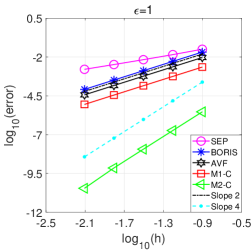
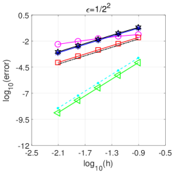
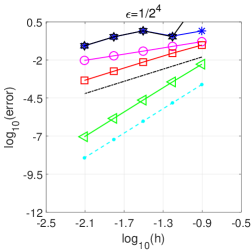
(i)	(ii)	(iii)

Figure 1: Problem 1. The global errors $error:=\frac{|x_{n}-x(t_{n})|}{|x(t_{n})|}+\frac{|v_{n}-v(t_{n})|}{|v(t_{n})|}$ with $t=10$ and $h=1/2^{k}$ for $k=3,...,7$ under different $\epsilon$.

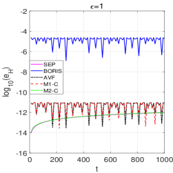
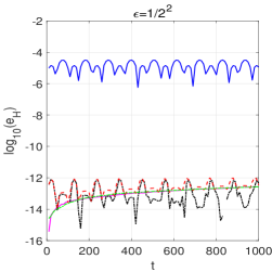
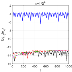
(i)	(ii)	(iii)

Figure 2: Problem 1. Evolution of the energy error $e_{H}:=\frac{|H(x_{n},v_{n})-H(x_{0},v_{0})|}{|H(x_{0},v_{0})|}$ as function of time $t=nh$.

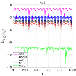
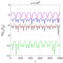
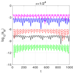
(i)	(ii)	(iii)

Figure 3: Problem 1. Evolution of the momentum error $e_{M}:=\frac{|M(x_{n},v_{n})-M(x_{0},v_{0})|}{|M(x_{0},v_{0})|}$ as function of time $t=nh$.

Problem 2. The second problem considers the charged-particle dynamics (1) from [16] in the constant magnetic field with $B=\frac{1}{2}(0.9,0.1,1)^{\intercal}$ and the scalar potential $U(x)=x_{1}^{3}-x_{2}^{3}+\frac{1}{5}x_{1}^{4}+x_{2}^{4}+x_{3}^{4}$. The initial values are chosen as $x(0)=(0,1.0,0.1)^{\intercal},v(0)=(0.09,0.55,0.3)^{\intercal}.$

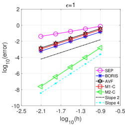
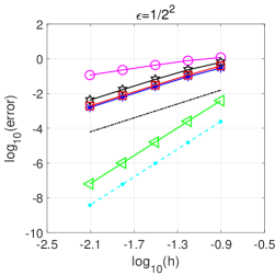
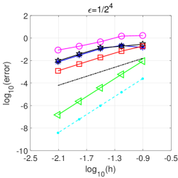
(i)	(ii)	(iii)

Figure 4: Problem 2. The global errors $error:=\frac{|x_{n}-x(t_{n})|}{|x(t_{n})|}+\frac{|v_{n}-v(t_{n})|}{|v(t_{n})|}$ with $t=10$ and $h=1/2^{k}$ for $k=3,...,7$ under different $\epsilon$.

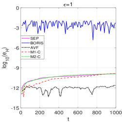
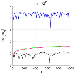
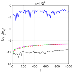
(i)	(ii)	(iii)

Figure 5: Problem 2. Evolution of the energy error $e_{H}:=\frac{|H(x_{n},v_{n})-H(x_{0},v_{0})|}{|H(x_{0},v_{0})|}$ as function of time $t=nh$.

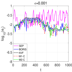
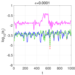
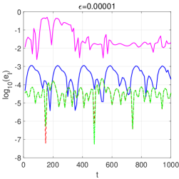
(i)	(ii)	(iii)

Figure 6: Problem 2. Evolution of the magnetic moment error $e_{I}:=\frac{|I(x_{n},v_{n})-I(x_{0},v_{0})|}{|I(x_{0},v_{0})|}$ as function of time $t=nh$.

The problem is solved on $[0,10]$ with different $\epsilon$ and $h=1/2^{k}$, where $k=3,...,7$. See Figure 4 for the global errors. Then we integrate the system with $h=\frac{1}{100}$ on $[0,1000]$. Figure 5 presents the energy conservation. Besides, we consider the magnetic moment

$$I(x,v)=\frac{\frac{1}{2}|\dot{x}\times B(x)|^{2}}{|B(x)|^{3}},$$

which is an adiabatic invariant of the system [2, 3, 16]. Its errors $e_{I}:=\frac{|I(x_{n},v_{n})-I(x_{0},v_{0})|}{|I(x_{0},v_{0})|}$ with $h=\frac{1}{100}$ on $[0,1000]$ are shown in Figure 6.

From the above two numerical results in Figures 1-6, we can draw the following conclusions.

1) From Figure 1 and Figure 4, we can see the global error lines of our methods M1-C and M2-C are respectively nearly parallel to the lines with slope 2 and slope 4, which shows that our methods M1-C and M2-C are second order and fourth order, respectively. Moreover, it can be seen that our methods M1-C and M2-C have better accuracy than the methods Boris, AVF and SEP in the literature.

2) The results in Figure 2 and Figure 5 are shown that the energy-preserving methods AVF, M1-C, M2-C and SEP have an excellent energy conservation. The boris method does not have such conservation.

3) For the magnetic moment conservation, it can be observed from Figure 3 that all the methods have a long-term conservation behaviour, and M2-C behaves much better than the others.

4) It can be observed from the results in Figure 6 that M1-C and M2-C have a long-term magnetic moment conservation when $\epsilon$ is small. Other methods do not show this near conservation and since the error of AVF is too large, we do not plot the corresponding results in the figure.

6 Extension to CPD in a nonuniform magnetic field

In this section, we shall extend the obtained integrators to solve the CPD (1) in a nonuniform magnetic field $B(x)=(B_{1}(x),B_{2}(x),B_{3}(x))^{\intercal}$, where $B_{i}(x):{\mathbb{R}}^{3}\rightarrow{\mathbb{R}}$ for $i=1,2,3.$

6.1 Integrators and their properties

Algorithm 6.1

For solving the CPD (1) in a nonuniform magnetic field $B(x)$, define the following continuous-stage exponential integrator

$$\left\{\begin{aligned} &X_{\tau}=x_{n}+h\tau\varphi_{1}(h\widetilde{K}_{n})v_{n}+h^{2}\int_{0}^{1}\tau\varphi_{2}(h\widetilde{K}_{n})F(X_{\sigma})d\sigma,\ \ \ 0\leq\tau\leq 1,\\ &x_{n+1}=x_{n}+h\varphi_{1}(h\widetilde{K}_{n})v_{n}+h^{2}\int_{0}^{1}\varphi_{2}(h\widetilde{K}_{n})F(X_{\tau})d\tau,\\ &v_{n+1}=\varphi_{0}(h\widetilde{K}_{n})v_{n}+h\int_{0}^{1}\varphi_{1}(h\widetilde{K}_{n})F(X_{\tau})d\tau,\end{aligned}\right.$$ (28)

where $h$ is the stepsize and $\widetilde{K}_{n}=\frac{1}{\epsilon}\widetilde{B}(\frac{x_{n}+x_{n+1}}{2})$. We shall refer to this integrator by M1-B.

Based on M1-B denoted by $\Phi_{h}$, we can obtain a Triple Jump splitting scheme [19]: $\Psi_{h}=\Phi_{a_{1}h}\circ\Phi_{a_{2}h}\circ\Phi_{a_{3}h}$, where $a_{1}=a_{3}=\frac{1}{2-\sqrt[3]{2}}$ and $a_{2}=-\frac{\sqrt[3]{2}}{2-\sqrt[3]{2}}$. We shall call this integrator M2-B.

For these two new integrators, they have the following propositions.

Proposition 6.2

$\bullet$ Both M1-B and M2-B are symmetric and exactly preserve the energy (2) of CPD, i.e.,

$$H(x_{n},v_{n})=H(x_{0},v_{0})\ \ \ \textmd{for}\ \ n=1,2,\ldots,T/h.$$

$\bullet$ The integrator M1-B is of order two and M2-B is of order four.

Proof.   $\bullet$ By replacing $K$ in the previous proof with $\widetilde{K}_{n}$ and with the same arguments as before, the symmetry and energy conservation of M1-B can be proved. Then using the symmetric splitting gives the structure conservations of M2-B immediately.

$\bullet$ According to the analysis of [40], it is known that the convergence of second-order integrator can be obtained by showing the errors when the considered integrator is applied to the linearized problem

$$\begin{array}[c]{ll}\ddot{\tilde{x}}(s)=\dot{\tilde{x}}(s)\times\frac{1}{\epsilon}\widetilde{B}(\frac{x_{n}+x_{n+1}}{2})+F(\tilde{x}(s)),\quad\tilde{x}(0)=x(t_{n}),\quad\dot{\tilde{x}}(t_{0})=\dot{x}(t_{n}),\ \ s\in[0,h],\end{array}$$

for some $t=t_{n}+s$ with $n\geq 0$. Under this case, by the variation-of-constants formula and the convergence analysis stated before, the second order convergence of M1-B can be established. Finally, Triple Jump splitting scheme acting on M1-B implies the fourth order accuracy of M2-B.

6.2 Numerical tests

In what follows, we carry out two numerical tests to show the behaviour of the above two methods. The methods chosen for comparison are still BORIS, AVF and SEP, which are given in Section 5. Problem 3. We consider the charged-particle dynamics (1) in the general magnetic field [17], and the potential $U(x)$ and field $B(x)$ are given by

$$U(x)=\frac{1}{100\sqrt{x_{1}^{2}+x_{2}^{2}}},\ \ \ B(x)=(0,0,\sqrt{x_{1}^{2}+x_{2}^{2}})^{\intercal},$$

where $B(x)=\nabla\times A(x)$ with $A(x)=\frac{1}{3}(-x_{2}\sqrt{x_{1}^{2}+x_{2}^{2}},x_{1}\sqrt{x_{1}^{2}+x_{2}^{2}},0)^{T}.$ We take the initial values as $x(0)=(0,1,0.1)^{\intercal},\ v(0)=(0.09,0.05,0.2)^{\intercal}.$ The problem is solved on $[0,10]$ with $h=1/2^{k},$ where $k=3,\ldots,7$. The global errors are presented in Figure 7. Then we solve the system with a step size $h=\frac{1}{100}$ on the interval $[0,1000]$. The results of energy and momentum are displayed in Figure 8 and Figure 9, respectively.

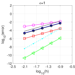
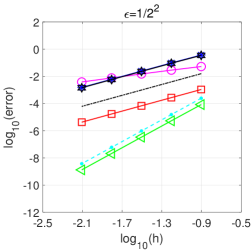
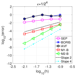
(i)	(ii)	(iii)

Figure 7: Problem 3. The global errors $error:=\frac{|x_{n}-x(t_{n})|}{|x(t_{n})|}+\frac{|v_{n}-v(t_{n})|}{|v(t_{n})|}$ with $t=10$ and $h=1/2^{k}$ for $k=3,...,7$ under different $\epsilon$.

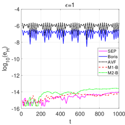
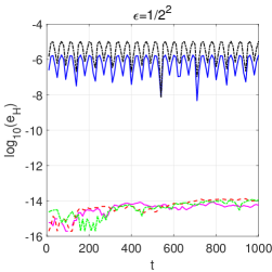
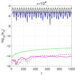
(i)	(ii)	(iii)

Figure 8: Problem 3. Evolution of the energy error $e_{H}:=\frac{|H(x_{n},v_{n})-H(x_{0},v_{0})|}{|H(x_{0},v_{0})|}$ as function of time $t=nh$.

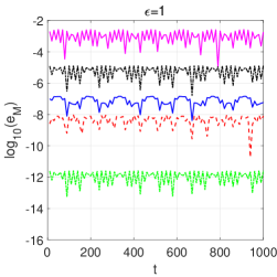
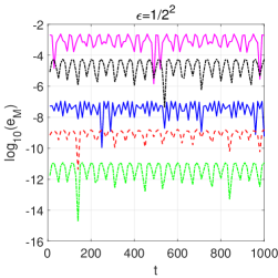
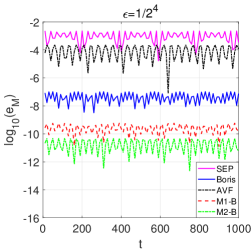
(i)	(ii)	(iii)

Figure 9: Problem 3. Evolution of the momentum error $e_{M}:=\frac{|M(x_{n},v_{n})-M(x_{0},v_{0})|}{|M(x_{0},v_{0})|}$ as function of time $t=nh$.

Problem 4. The last test is devoted to charged-particle dynamics (1) with the general magnetic field [16]

$$B(x)=\nabla\times\frac{1}{4}(x_{3}^{2}-x_{2}^{2},x_{3}^{2}-x_{1}^{2},x_{2}^{2}-x_{1}^{2})^{\intercal}=\frac{1}{2}(x_{2}-x_{3},x_{1}+x_{3},x_{2}-x_{1})^{\intercal},$$

and the scalar potential $U(x)=x_{1}^{3}-x_{2}^{3}+\frac{1}{5}x_{1}^{4}+x_{2}^{4}+x_{3}^{4}.$ The initial values are chosen as $x(0)=(0.0,1.0,0.1)^{\intercal},\ v(0)=(0.09,0.55,0.30)^{\intercal}.$ This system is integrated on $[0,10]$ with different $\epsilon$ and $h=1/2^{k}$, where $k=3,...,7$, and see Figure 10 for the errors. Then we solve the problem with $h=\frac{1}{100}$ on $[0,1000]$. Figure 11 and Figure 12 display the errors $e_{H}$ of the energy and $e_{I}$ of the magnetic moment, respectively.

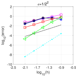
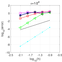
(i)	(ii)	(iii)

Figure 10: Problem 4. The global errors $error:=\frac{|x_{n}-x(t_{n})|}{|x(t_{n})|}+\frac{|v_{n}-v(t_{n})|}{|v(t_{n})|}$ with $t=10$ and $h=1/2^{k}$ for $k=3,...,7$ under different $\epsilon$.

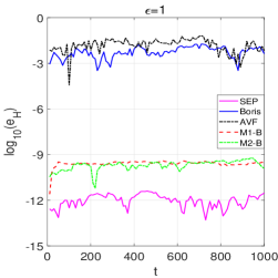
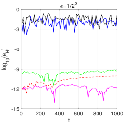
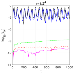
(i)	(ii)	(iii)

Figure 11: Problem 4. Evolution of the energy error $e_{H}:=\frac{|H(x_{n},v_{n})-H(x_{0},v_{0})|}{|H(x_{0},v_{0})|}$ as function of time $t=nh$.

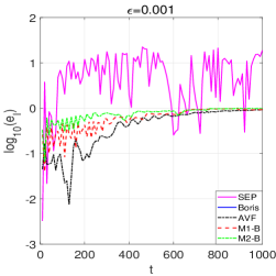
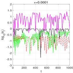
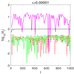
(i)	(ii)	(iii)

Figure 12: Problem 4. Evolution of the magnetic moment error $e_{I}:=\frac{|I(x_{n},v_{n})-I(x_{0},v_{0})|}{|I(x_{0},v_{0})|}$ as function of time $t=nh$.

From the results of these two tests, it can be observed that AVF is no longer energy preserving and other numerical phenomena are similar as Problems 1-2. In conclusion, the M1-C and M2-C respectively show second order and fourth order in the accuracy, conserve the energy with good accuracy and have long time near conservations in the momentum and magnetic moment (when $\varepsilon$ is small). The theoretical analysis of the near conservation in the momentum and magnetic moment will be considered in our next work.

7 Conclusions

In this paper, geometric continuous-stage exponential energy-preserving integrators for the charged-particle dynamics (CPD) (1) were formulated and developed. The novel integrators were designed for the CPD in a magnetic field from normal to strong regimes, and they work well for these both regimes. We analysed the energy-preserving conditions, symmetric conditions and order conditions for the novel integrators. Using these results, two symmetric continuous-stage exponential energy-preserving schemes of order up to four were constructed. The numerical experiments were performed and the results showed that our novel methods were more effective than some existing methods in the literature.

Last but not least, it is noted that the accuracy of the proposed integrators of this paper is not uniform in $\epsilon$ which is different from the uniformly accurate methods [8, 9, 10, 12]. The formulation of uniformly accurate methods with exact energy conservation is interesting but very challenging. Very recently, the work [41] succeeded in equipping the favorable uniformly accuracy methods with near conservation laws in long times. We hope to make some progress on the topic of energy-preserving uniformly accurate methods in our future work.

References

- [1] V. I. Arnold, Mathematical Methods of Classical Mechanics, Graduate Texts in Mathematics, Springer-Verlag, 1978.
- [2] V. I. Arnold, V. V. Kozlov, A. I. Neishtadt, Mathematical Aspects of Classical and Celestial Mechanics, Springer, Berlin, 1997.
- [3] G. Benettin, P. Sempio, Adiabatic invariants and trapping of a point charge in a strong nonuniform magnetic field, Nonlinearity, 7 (1994) 281-304.
- [4] J. P. Boris, Relativistic plasma simulation-optimization of a hybird code, Proceeding of Fourth Conference on Numerical Simulations of Plasmas, 11(1970) 3-67.
- [5] A. J. Brizard, T. S. Hahm, Foundations of nonlinear gyrokinetic theory, Rev. Modern Phys. 79 (2007) 421-468.
- [6] L. Brugnano, F. Iavernaro, R. Zhang, Arbitrarily high-order energy-preserving methods for simulating the gyrocenter dynamics of charged particles, J. Comput. Appl. Math. 380 (2020) 112994.
- [7] L. Brugnano, J. I. Montijano, L. Rándz, High-order energy-conserving line integral methods for charged particle dynamics, J. Comput Phys. 396 (2019) 209-227.
- [8] Ph. Chartier, N. Crouseilles, M. Lemou, F. Méhats, X. Zhao, Uniformly accurate methods for Vlasov equations with non-homogeneous strong magnetic field, Math. Comp. 88 (2019) 2697-2736.
- [9] Ph. Chartier, N. Crouseilles, M. Lemou, F. Méhats, X. Zhao, Uniformly accurate methods for three dimensional Vlasov equations under strong magnetic field with varying direction, SIAM J. Sci. Compt. 42 (2020) B520-B547.
- [10] N. Crouseilles, M. Lemou, F. Méhats, X. Zhao, Uniformly accurate Particle-in-Cell method for the long time two-dimensional Vlasov-Poisson equation with uniform strong magnetic field, J. Comput. Phys. 346 (2017) 172-190.
- [11] F. Filbet, T. Xiong, E. Sonnendrücker, On the Vlasov-Maxwell system with a strong magnetic field, SIAM J. Appl. Math. 78 (2018) 1030-1055.
- [12] E. Frénod, S. A. Hirstoaga, M. Lutz, E. Sonnendrücker, Long time behavior of an exponential integrator for a Vlasov-Poisson system with strong magnetic field, Commun. Comput. Phys. 18 (2015) 263-296.
- [13] E. Frénod, S. A. Hirstoaga, E. Sonnendrücker, An exponential integrator for a highly oscillatory vlasov equation, Disc. cont. dyn. syst. series S 8 (2015) 169–183.
- [14] E. Hairer, Energy-preserving variant of collocation methods, J. Numer. Anal. Ind. Appl. Math. 5 (2010) 73-84.
- [15] E. Hairer, Ch. Lubich, Energy behaviour of the Boris method for charged-particle dynamics, BIT 58 (2018) 969-979.
- [16] E. Hairer, Ch. Lubich, Long-term analysis of a variational integrator for charged-particle dynamics in a strong magnetic field, Numer. Math. 144 (2020) 699-728.
- [17] E. Hairer, Ch. Lubich, Symmetric multistep methods for charged-particle dynamics, SMAI J. Comput. Math. 3 (2017) 205-218.
- [18] E. Hairer, Ch. Lubich, B. Wang, A filtered Boris algorithm for charged-particle dynamics in a strong magnetic field, Numer. Math. 144 (2020) 787-809.
- [19] E. Hairer, Ch. Lubich, G. Wanner, Geometric Numerical Integration: Structure-Preserving Algorithms for Ordinary Differential Equations, 2nd edn. Springer-V erlag, Berlin, Heidelberg, 2006.
- [20] Y. He, Y. Sun, J. Liu, H. Qin, Volume-preserving algorithms for charged particle dynamics, J. Comput. Phys. 281 (2015) 135-147.
- [21] M. Hochbruck, A. Ostermann, Explicit exponential Runge–Kutta methods for semilineal parabolic problems, SIAM J. Numer. Anal. 43 (2005) 1069-1090.
- [22] M. Hochbruck, A. Ostermann, Exponential integrators, Acta Numer. 19 (2010) 209-286.
- [23] M. Hochbruck, A. Ostermann, J. Schweitzer, Exponential rosenbrock-type methods, SIAM J. Numer. Anal. 47 (2009) 786-803.
- [24] K. Kormann, E. Sonnendrücker, Energy-conserving time propagation for a structure-preserving particle-in-cell Vlasov-Maxwell solver, J. Comput. Phys. 425 (2021) 109890.
- [25] T. Li, B. Wang, Eficient energy-reserving methods for chrged-particle dynamics, Appl. Math. Comput. 361 (2019) 703-714.
- [26] X. Li, B. Wang, Energy-preserving splitting methods for charged partícle dynamics in a normal or strong magnetic field, Appl. Math. Lett. 124 (2022) 107682.
- [27] E. Madaule, M. Restelli, E. Sonnendrücker, Energy conserving discontinuous Galerkin spectral element method for the Vlasov-Poisson system. J. Comput. Phys. 279 (2014) 261–188.
- [28] R. I. McLachlan, G. R. W. Quispel, N. Robidoux, Geometric integration using discrete gradient, Philos. Trans. R. Soc. Lond. A 357 (1999) 1021-1045.
- [29] L. Mei, X. Wu, Symplectic exponential Runge–Kutta methods for solving nonlinear Hamiltonian systems, J. Comput. Phys. 338 (2017) 567-584.
- [30] Y. Miyatake, J. C. Butcher, Characterization of enegy-preserving methods and the construction of parallel integrators for Hamiltonian systems. SIAM J. Numer. Anal. 54 (2016) 1993-2013.
- [31] B. Perse, K. Kormann, E. Sonnendrücker, Geometric Particle-in-Cell Simulations of the Vlasov–Maxwell System in Curvilinear Coordinates. SIAM J. Sci. Comput. 43 (2021) B194-B218.
- [32] S. Possanner, Gyrokinetics from variational averaging: existence and error bounds, J. Math. Phys. 59 (2018) 082702, 34.
- [33] H. Qin, S. Zhang, J. Xiao, J. Liu, Y. Sun, W. M. Tang, Why is Boris algorithm so good? Physics of Plasmas, 20 (2013) 084503.
- [34] L. F. Ricketson, L. Chacón, An energy conserving and asymptotic preserving charged-particle orbit implicit time integratorfor arbitrary electromagnetic fields, J. Comput. Phys. 418 (2020) 109639.
- [35] W. S. Tang, J. J. Zhang, Symplecticity-preserving continuous-stage Runge-Kutta-Nystrm methods. Appl. Math. Comput. 323 (2018) 204-219.
- [36] M. Tao, Explicit high-order symplectic integrators for charged particles in general electromagnetic fileds, J. Comput. Phys. 327 (2016) 245-251.
- [37] B. Wang, Exponential energy-preserving methods for charged particle dynamics in a strong and constant magnetic field, J. Comput. Appl. Math. 387 (2021) 112617.
- [38] B. Wang, X. Wu, Y. Fang, A two-step symmetric method for charged-particle dynamics in a normal or strong magnetic feld, Calcolo, 57 (2020) 29.
- [39] B. Wang, X. Wu, Y. Fang, A continuous-stage modified Leap-frog scheme for high dimensional semi-linear Hamiltonian wave equations, Numer. Math. Theo. Meth. Appl. 13 (2020) 814-844.
- [40] B. Wang, X. Zhao, Error estimates of some splitting schemes for charged-particle dynamics under strong magnetic field, SIAM J. Numer. Anal. 59 (2021) 2075-2105.
- [41] B. Wang, X. Zhao, Geometric two-scale integrators for highly oscillatory system: uniform accuracy and near conservations, arXiv.2110.15265
- [42] R. Zhang, H. Qin, Y. Tang, J. Liu, Y. He, J. Xiao, Explicit symplectic algorithms based on generating functions for charged particle dynamics, Phys. Revi. E 94 (2016) 013205.