Randomized regularized extended Kaczmarz algorithms for tensor recovery

Abstract

Randomized regularized Kaczmarz algorithms have recently been proposed to solve tensor recovery models with consistent linear measurements. In this work, we propose a novel algorithm based on the randomized extended Kaczmarz algorithm (which converges linearly in expectation to the unique minimum norm least squares solution of a linear system) for tensor recovery models with inconsistent linear measurements. We prove the linear convergence in expectation of our algorithm. Numerical experiments on a tensor least squares problem and a sparse tensor recovery problem are given to illustrate the theoretical results.

Keywords. Randomized regularized extended Kaczmarz, sparse tensor recovery, tensor least squares problem, linear convergence

AMS subject classifications: 65F10, 68W20, 90C25, 15A69

1 Introduction

Tensor recovery models have attracted much attention recently because of various applications, such as transportation, medical imaging, and remote sensing. With the assumption of consistent linear measurements, Chen and Qin [7] proposed a algorithmic framework based on the Kaczmarz-type algorithms [12, 29] for the following tensor recovery model:

$$\widehat{\mathcal{X}}=\operatorname*{argmin}_{\mathcal{X}\in\mathbb{R}^{N_{2}\times K\times N_{3}}}f(\mathcal{X}),\quad\mbox{s.t.}\quad\mathcal{A}*\mathcal{X}=\mathcal{B},$$ (1)

where the objective function $f$ is strongly convex, the sensing tensor $\mathcal{A}\in\mathbb{R}^{N_{1}\times N_{2}\times N_{3}}$, the acquired measurement tensor $\mathcal{B}\in\mathbb{R}^{N_{1}\times K\times N_{3}}$, and $\mathcal{A}*\mathcal{X}$ is the tensor t-product [14]. In this paper, we assume that the linear measurement $\mathcal{A}*\mathcal{X}=\mathcal{B}$ is inconsistent and therefore consider the following constrained minimization problem:

$$\widehat{\mathcal{X}}=\operatorname*{argmin}_{\mathcal{X}\in\mathbb{R}^{N_{2}\times K\times N_{3}}}f(\mathcal{X}),\quad\mbox{s.t.}\quad\mathcal{A}^{\top}*\mathcal{A}*\mathcal{X}=\mathcal{A}^{\top}*\mathcal{B},$$ (2)

where $\mathcal{A}^{\top}$ denotes the transpose of $\mathcal{A}$ (see section 2.1). The solution $\widehat{\mathcal{X}}$ of (2) is a least squares solution of the inconsistent system $\mathcal{A}*\mathcal{X}=\mathcal{B}$ with some desirable characteristics promoted by regularization terms of the objective function $f$.

In recent years, randomized iterative algorithms for linear systems of equations with massive data sets have been greatly developed due to low memory footprints and good numerical performance, such as the randomized Kaczmarz (RK) algorithm [29], the randomized coordinate descent (RCD) algorithm [16], the randomized extended Kaczmarz (REK) algorithm [35], and their extensions, e.g., [24, 10, 20, 25, 1, 2, 3, 8, 22, 9, 4, 31, 32, 11, 33]. The RK algorithm converges linearly in expectation to a solution of consistent linear systems [29, 35] and to within a radius (convergence horizon) of a (least squares) solution of inconsistent linear systems [23]. The REK algorithm converges linearly in expectation to a (least squares) solution of arbitrary linear systems [35, 20, 8]. In this paper, we replace the RK algorithm integrated in the randomized regularized Kaczmarz (RRK) algorithm of [7, Algorithm 3.2] with the REK algorithm and propose a randomized regularized extended Kaczmarz (RREK) algorithm for solving (2). The proposed RREK algorithm is called “regularized” since the objective function contains regularization terms for preserving some desirable characteristics of the underlying solution. We prove the linear convergence of the proposed algorithm. Special cases including tensor least squares problems and sparse tensor recovery problems are provided. Numerical experiments are given to illustrate our theoretical results.

The rest of this paper is organized as follows. In section 2, we provide clarification of notation, review basic concepts and results in tensor algebra and convex optimization, and also briefly introduce the RRK algorithm of [7]. In section 3, we describe the proposed RREK algorithm for solving (2) and establish its convergence theory. In section 4, we discuss two special cases including a tensor least squares problem and a sparse tensor recovery problem. In section 5, we report two numerical experiments to illustrate the theoretical results. Finally, we present brief concluding remarks in section 6.

2 Preliminaries

2.1 Basic notation

Throughout the paper, we use boldface uppercase letters such as $\mathbf{A}$ for matrices and calligraphic letters such as $\mathcal{A}$ for tensors. For an integer $m\geq 1$, let $[m]:=\{1,2,3,\ldots,m\}$. For any matrix $\mathbf{A}\in\mathbb{R}^{m\times n}$, we use $\mathbf{A}^{\top}$, $\mathbf{A}^{\dagger}$, $\|\mathbf{A}\|_{2}$, and $\sigma_{\rm min}(\mathbf{A})$ to denote the transpose, the Moore–Penrose pseudoinverse, the spectral norm, and the minimum nonzero singular values of $\mathbf{A}$, respectively. For any random variables $\bm{\xi}$ and $\bm{\zeta}$, we use $\mathbb{E}\begin{bmatrix}\bm{\xi}\end{bmatrix}$ and $\mathbb{E}\begin{bmatrix}\bm{\xi}\mid\bm{\zeta}\end{bmatrix}$ to denote the expectation of $\bm{\xi}$ and the conditional expectation of $\bm{\xi}$ given $\bm{\zeta}$, respectively.

2.2 Tensor basics

In this subsection, we provide a brief review of key definitions and facts in tensor algebra. We follow the notation used in [14, 13, 21].

For a third-order tensor $\mathcal{A}\in\mathbb{R}^{N_{1}\times N_{2}\times N_{3}}$, we denote its $(i,j,k)$ entry as $\mathcal{A}_{ijk}$ and use $\mathcal{A}_{i,:,:}$, $\mathcal{A}_{:,i,:}$ and $\mathcal{A}_{:,:,i}$ to denote respectively the $i$th horizontal, lateral and frontal slice. For notational convenience, the $i$th frontal slice $\mathcal{A}_{:,:,i}$ will be denoted as $\mathbf{A}_{i}$. We define the block circulant matrix ${\rm bcirc}(\mathcal{A})$ of $\mathcal{A}$ as,

$${\rm bcirc}(\mathcal{A}):=\begin{bmatrix}\mathbf{A}_{1}&\mathbf{A}_{N_{3}}&\cdots&\mathbf{A}_{2}\\ \mathbf{A}_{2}&\mathbf{A}_{1}&\cdots&\mathbf{A}_{3}\\ \vdots&\vdots&\ddots&\vdots\\ \mathbf{A}_{N_{3}}&\mathbf{A}_{N_{3}-1}&\cdots&\mathbf{A}_{1}\end{bmatrix}\in\mathbb{R}^{N_{1}N_{3}\times N_{2}N_{3}}.$$

We also define the operator ${\rm unfold}(\cdot)$ and its inversion ${\rm fold}(\cdot)$,

$${\rm unfold}(\mathcal{A}):=\begin{bmatrix}\mathbf{A}_{1}\\ \mathbf{A}_{2}\\ \vdots\\ \mathbf{A}_{N_{3}}\end{bmatrix}\in\mathbb{R}^{N_{1}N_{3}\times N_{2}},\qquad{\rm fold}\left(\begin{bmatrix}\mathbf{A}_{1}\\ \mathbf{A}_{2}\\ \vdots\\ \mathbf{A}_{N_{3}}\end{bmatrix}\right):=\mathcal{A}.$$

Definition 2.1 (t-product).

For $\mathcal{A}\in\mathbb{R}^{N_{1}\times N_{2}\times N_{3}}$ and $\mathcal{B}\in\mathbb{R}^{N_{2}\times K\times N_{3}}$, the t-product $\mathcal{A}*\mathcal{B}$ is defined to be a tensor of size $N_{1}\times K\times N_{3}$,

$$\mathcal{A}*\mathcal{B}:={\rm fold}({\rm bcirc}(\mathcal{A}){\rm unfold}(\mathcal{B})).$$

Definition 2.2 (transpose).

The transpose of $\mathcal{A}\in\mathbb{R}^{N_{1}\times N_{2}\times N_{3}}$, denoted by $\mathcal{A}^{\top}$, is the $N_{2}\times N_{1}\times N_{3}$ tensor obtained by transposing each of the frontal slices and then reversing the order of transposed frontal slices $2$ through $N_{3}$.

For $\mathcal{A}\in\mathbb{R}^{N_{1}\times N_{2}\times N_{3}}$, we have

$${\rm bcirc}(\mathcal{A}^{\top})=({\rm bcirc}(\mathcal{A}))^{\top}.$$ (3)

Definition 2.3 (identity tensor).

The identity tensor $\mathcal{I}\in\mathbb{R}^{N\times N\times N_{3}}$ is the tensor whose first frontal slice is the $N\times N$ identity matrix, and whose other frontal slices are all zeros.

For $\mathcal{A}\in\mathbb{R}^{N_{1}\times N_{2}\times N_{3}}$ and $\mathcal{I}\in\mathbb{R}^{N_{1}\times N_{1}\times N_{3}}$, it holds that

$$\mathcal{A}_{i,:,:}=\mathcal{I}_{i,:,:}*\mathcal{A}.$$ (4)

For $\mathcal{A}\in\mathbb{R}^{N_{1}\times N_{2}\times N_{3}}$ and $\mathcal{I}\in\mathbb{R}^{N_{2}\times N_{2}\times N_{3}}$, it holds that

$$\mathcal{A}_{:,j,:}=\mathcal{A}*\mathcal{I}_{:,j,:}.$$ (5)

Definition 2.4 (inner product).

The inner product between $\mathcal{A}$ and $\mathcal{B}$ in $\mathbb{R}^{N_{1}\times N_{2}\times N_{3}}$ is defined as

$$\langle\mathcal{A},\mathcal{B}\rangle:=\sum_{i,j,k}\mathcal{A}_{ijk}\mathcal{B}_{ijk}.$$

For $\mathcal{A}\in\mathbb{R}^{N_{1}\times N_{2}\times N_{3}}$, $\mathcal{B}\in\mathbb{R}^{N_{2}\times K\times N_{3}}$, and $\mathcal{C}\in\mathbb{R}^{N_{1}\times K\times N_{3}}$, it holds that

$$\langle\mathcal{A}*\mathcal{B},\mathcal{C}\rangle=\langle\mathcal{B},\mathcal{A}^{\top}*\mathcal{C}\rangle.$$ (6)

Definition 2.5 ($1$-norm, spectral norm, and Frobenius norm).

The 1-norm, spectral norm, and Frobenius norm of $\mathcal{A}\in\mathbb{R}^{N_{1}\times N_{2}\times N_{3}}$ are defined as

$$\|\mathcal{A}\|_{1}:=\sum_{i,j,k}|\mathcal{A}_{ijk}|,\qquad\|\mathcal{A}\|_{2}:=\|{\rm bcirc}(\mathcal{A})\|_{2},$$

and

$$\|\mathcal{A}\|_{\rm F}:=\sqrt{\langle\mathcal{A},\mathcal{A}\rangle}=\sqrt{\sum_{i,j,k}(\mathcal{A}_{ijk})^{2}},$$

respectively.

For $\mathcal{A}$ and $\mathcal{B}$ in $\mathbb{R}^{N_{1}\times N_{2}\times N_{3}}$, it holds that

$$|\langle\mathcal{A},\mathcal{B}\rangle|\leq\|\mathcal{A}\|_{\rm F}\|\mathcal{B}\|_{\rm F}.$$ (7)

For $\mathcal{A}\in\mathbb{R}^{N_{1}\times N_{2}\times N_{3}}$ and $\mathcal{B}\in\mathbb{R}^{N_{2}\times K\times N_{3}}$, it holds that

$$\|\mathcal{A}*\mathcal{B}\|_{\rm F}\leq\|\mathcal{A}\|_{2}\|\mathcal{B}\|_{\rm F}.$$ (8)

Definition 2.6 ($K$-range).

The $K$-range of $\mathcal{A}\in\mathbb{R}^{N_{1}\times N_{2}\times N_{3}}$ is defined as

$${\rm range}_{K}(\mathcal{A}):=\{\mathcal{A}*\mathcal{Y}\mid\mathcal{Y}\in\mathbb{R}^{N_{2}\times K\times N_{3}}\}.$$

For $\mathcal{A}\in\mathbb{R}^{N_{1}\times N_{2}\times N_{3}}$, it holds that

$${\rm range}_{K}(\mathcal{A}^{\top}*\mathcal{A})={\rm range}_{K}(\mathcal{A}^{\top}).$$

For $\mathcal{A}\in\mathbb{R}^{N_{1}\times N_{2}\times N_{3}}$ and all $\mathcal{X}\in{\rm range}_{K}(\mathcal{A})$, it holds that

$$\|\mathcal{A}^{\top}*\mathcal{X}\|_{\rm F}^{2}\geq\sigma_{\min}^{2}({\rm bcirc}(\mathcal{A}))\|\mathcal{X}\|_{\rm F}^{2}.$$ (9)

Definition 2.7 (pseudoinverse).

The pseudoinverse of $\mathcal{A}\in\mathbb{R}^{N_{1}\times N_{2}\times N_{3}}$, denoted by $\mathcal{A}^{\dagger}$, is the $N_{2}\times N_{1}\times N_{3}$ tensor satisfying

$${\rm bcirc}(\mathcal{A}^{\dagger})={\rm bcirc}(\mathcal{A})^{\dagger}.$$

For $\mathcal{A}\in\mathbb{R}^{N_{1}\times N_{2}\times N_{3}}$ and $\mathcal{B}\in\mathbb{R}^{N_{1}\times K\times N_{3}}$, it holds that

$$\mathcal{A}^{\top}*\mathcal{A}*\mathcal{A}^{\dagger}*\mathcal{B}=\mathcal{A}^{\top}*\mathcal{B}.$$

If $\mathcal{X}\in\mathbb{R}^{N_{2}\times K\times N_{3}}$ satisfies $\mathcal{A}^{\top}*\mathcal{A}*\mathcal{X}=\mathcal{A}^{\top}*\mathcal{B}$, then it holds that

$$\mathcal{A}*\mathcal{X}=\mathcal{A}*\mathcal{A}^{\dagger}*\mathcal{B}.$$

2.3 Convex optimization basics

To make the paper self-contained, we present basic definitions and properties about convex functions defined on tensor spaces in this subsection. We refer the reader to [26, 5] for more definitions and properties.

Definition 2.8 (subdifferential).

For a continuous function $f:\mathbb{R}^{N_{1}\times N_{2}\times N_{3}}\rightarrow\mathbb{R}$, its subdifferential at $\mathcal{X}\in\mathbb{R}^{N_{1}\times N_{2}\times N_{3}}$ is defined as

$$\partial f(\mathcal{X}):=\{\mathcal{Z}:f(\mathcal{Y})\geq f(\mathcal{X})+\langle\mathcal{Z},\mathcal{Y}-\mathcal{X}\rangle\quad\forall\ \mathcal{Y}\in\mathbb{R}^{N_{1}\times N_{2}\times N_{3}}\}.$$

Definition 2.9 ($\gamma$-strong convexity).

A function $f:\mathbb{R}^{N_{1}\times N_{2}\times N_{3}}\rightarrow\mathbb{R}$ is called $\gamma$-strongly convex for a given $\gamma>0$ if the following inequality holds for all $\mathcal{X},\mathcal{Y}\in\mathbb{R}^{N_{1}\times N_{2}\times N_{3}}$ and $\mathcal{Z}\in\partial f(\mathcal{X})$:

$$f(\mathcal{Y})\geq f(\mathcal{X})+\langle\mathcal{Z},\mathcal{Y}-\mathcal{X}\rangle+\frac{\gamma}{2}\|\mathcal{Y}-\mathcal{X}\|_{\rm F}^{2}.$$

The function $f(\mathcal{X})=\displaystyle\frac{1}{2}\|\mathcal{X}\|_{\rm F}^{2}$ is differential and $1$-strongly convex. Moreover, it is easy to show that the function $h(\mathcal{X})+\displaystyle\frac{1}{2}\|\mathcal{X}\|_{\rm F}^{2}$ is $1$-strongly convex if $h(\mathcal{X})$ is convex.

Definition 2.10 (conjugate function).

The conjugate function of $f:\mathbb{R}^{N_{1}\times N_{2}\times N_{3}}\rightarrow\mathbb{R}$ at $\mathcal{Y}\in\mathbb{R}^{N_{1}\times N_{2}\times N_{3}}$ is defined as

$$f^{*}(\mathcal{Y}):=\sup_{\mathcal{X}\in\mathbb{R}^{N_{1}\times N_{2}\times N_{3}}}\{\langle\mathcal{Y},\mathcal{X}\rangle-f(\mathcal{X})\}.$$

If $f(\mathcal{X})$ is $\gamma$-strongly convex, then the conjugate function $f^{*}(\mathcal{X})$ is differentiable and for all $\mathcal{X},\mathcal{Y}\in\mathbb{R}^{N_{1}\times N_{2}\times N_{3}}$, the following inequality holds:

$$f^{*}(\mathcal{Y})\leq f^{*}(\mathcal{X})+\langle\nabla f^{*}(\mathcal{X}),\mathcal{Y}-\mathcal{X}\rangle+\frac{1}{2\gamma}\|\mathcal{Y}-\mathcal{X}\|_{\rm F}^{2}.$$ (10)

For a strongly convex function $f(\mathcal{X})$, it can be shown that [26, 5]

$$\mathcal{Z}\in\partial f(\mathcal{X})\ \Leftrightarrow\ \mathcal{X}=\nabla f^{*}(\mathcal{Z}).$$ (11)

For a convex function $h(\mathcal{X})$, the conjugate function of $\lambda h(\mathcal{X})+\displaystyle\frac{1}{2}\|\mathcal{X}\|_{\rm F}^{2}$ is differentiable. Its gradient involves the proximal mapping of $h(\mathcal{X})$, and it holds that

$$\nabla\left(\lambda h(\cdot)+\frac{1}{2}\|\cdot\|_{\rm F}^{2}\right)^{*}(\mathcal{X})={\rm prox}_{\lambda h}(\mathcal{X}):=\operatorname*{argmin}_{\mathcal{Y}\in\mathbb{R}^{N_{1}\times N_{2}\times N_{3}}}\left\{\lambda h(\mathcal{Y})+\frac{1}{2}\|\mathcal{X}-\mathcal{Y}\|_{\rm F}^{2}\right\}.$$

Definition 2.11 (Bregman distance).

For a convex function $f:\mathbb{R}^{N_{1}\times N_{2}\times N_{3}}\rightarrow\mathbb{R}$, the Bregman distance between $\mathcal{X}$ and $\mathcal{Y}$ with respect to $f$ and $\mathcal{Z}\in\partial f(\mathcal{X})$ is defined as

$$D_{f,\mathcal{Z}}(\mathcal{X},\mathcal{Y}):=f(\mathcal{Y})-f(\mathcal{X})-\langle\mathcal{Z},\mathcal{Y}-\mathcal{X}\rangle.$$

It follows from $\langle\mathcal{Z},\mathcal{X}\rangle=f(\mathcal{X})+f^{*}(\mathcal{Z})$ if $\mathcal{Z}\in\partial f(\mathcal{X})$ that

$$D_{f,\mathcal{Z}}(\mathcal{X},\mathcal{Y})=f(\mathcal{Y})+f^{*}(\mathcal{Z})-\langle\mathcal{Z},\mathcal{Y}\rangle.$$ (12)

If $f$ is $\gamma$-strongly convex, then it holds that

$$D_{f,\mathcal{Z}}(\mathcal{X},\mathcal{Y})\geq\frac{\gamma}{2}\|\mathcal{X}-\mathcal{Y}\|_{\rm F}^{2}.$$ (13)

Definition 2.12 (restricted strong convexity [15, 27]).

Let $f:\mathbb{R}^{N_{1}\times N_{2}\times N_{3}}\rightarrow\mathbb{R}$ be convex differentiable with a nonempty minimizer set $X_{f}$. The function $f$ is called restricted strongly convex on $\mathbb{R}^{N_{1}\times N_{2}\times N_{3}}$ with a constant $\mu>0$ if it satisfies for all $\mathcal{X}\in\mathbb{R}^{N_{1}\times N_{2}\times N_{3}}$ the inequality

$$\langle\nabla f(P_{X_{f}}(\mathcal{X}))-\nabla f(\mathcal{X}),P_{X_{f}}(\mathcal{X})-\mathcal{X}\rangle\geq\mu\|P_{X_{f}}(\mathcal{X})-\mathcal{X}\|_{\rm F}^{2},$$

where $P_{X_{f}}(\mathcal{X})$ denotes the orthogonal projection of $\mathcal{X}$ onto $X_{f}$.

Definition 2.13 (strong admissibility).

Let $\mathcal{A}\in\mathbb{R}^{N_{1}\times N_{2}\times N_{3}}$ and $\mathcal{B}\in\mathbb{R}^{N_{1}\times K\times N_{3}}$ be given. Let $f:\mathbb{R}^{N_{2}\times K\times N_{3}}\rightarrow\mathbb{R}$ be strongly convex. The function $f$ is called strongly admissible if the function $g(\mathcal{Y}):=f^{*}(\mathcal{A}^{\top}*\mathcal{A}*\mathcal{Y})-\langle\mathcal{Y},\mathcal{A}^{\top}*\mathcal{B}\rangle$ is restricted strongly convex on $\mathbb{R}^{N_{2}\times K\times N_{3}}$.

Lemma 2.14.

Let $\widehat{\mathcal{X}}$ be the solution of (2). If $f$ is strongly admissible, then there exists a constant $\nu>0$ such that

$$D_{f,\mathcal{Z}}(\mathcal{X},\widehat{\mathcal{X}})\leq\frac{1}{\nu}\|\mathcal{A}*(\mathcal{X}-\widehat{\mathcal{X}})\|_{\rm F}^{2},$$ (14)

for all $\mathcal{X}\in\mathbb{R}^{N_{2}\times K\times N_{3}}$ and $\mathcal{Z}\in\partial f(\mathcal{X})\cap{\rm range}_{K}(\mathcal{A}^{\top})$.

Proof.

The solution $\widehat{\mathcal{X}}$ of (2) satisfies the following optimality conditions:

$$\mathcal{A}^{\top}*\mathcal{A}*\widehat{\mathcal{X}}=\mathcal{A}^{\top}*\mathcal{B},\qquad\partial f(\widehat{\mathcal{X}})\cap{\rm range}_{K}(\mathcal{A}^{\top}*\mathcal{A})\neq\emptyset.$$ (15)

The dual problem of (2) is the unconstrained problem

$$\min_{\mathcal{Y}\in\mathbb{R}^{N_{2}\times K\times N_{3}}}g(\mathcal{Y}),$$

where

$$g(\mathcal{Y})=f^{*}(\mathcal{A}^{\top}*\mathcal{A}*\mathcal{Y})-\langle\mathcal{Y},\mathcal{A}^{\top}*\mathcal{B}\rangle.$$

By the strong duality, we have

$$f(\widehat{\mathcal{X}})=-\min_{\mathcal{Y}\in\mathbb{R}^{N_{2}\times K\times N_{3}}}g(\mathcal{Y}).$$

Since $\mathcal{Z}\in{\rm range}_{K}(\mathcal{A}^{\top})={\rm range}_{K}(\mathcal{A}^{\top}*\mathcal{A})$, we can write $\mathcal{Z}=\mathcal{A}^{\top}*\mathcal{A}*\mathcal{Y}$ for some $\mathcal{Y}$. Then

$$D_{f,\mathcal{Z}}(\mathcal{X},\widehat{\mathcal{X}}) \stackrel{{\scriptstyle(\ref{dfz})}}{{=}}f^{*}(\mathcal{Z})-\langle\mathcal{Z},\widehat{\mathcal{X}}\rangle+f(\widehat{\mathcal{X}})$$

$$=f^{*}(\mathcal{A}^{\top}*\mathcal{A}*\mathcal{Y})-\langle\mathcal{A}^{\top}*\mathcal{A}*\mathcal{Y},\widehat{\mathcal{X}}\rangle+f(\widehat{\mathcal{X}})$$

$$\stackrel{{\scriptstyle(\ref{tran})}}{{=}}f^{*}(\mathcal{A}^{\top}*\mathcal{A}*\mathcal{Y})-\langle\mathcal{Y},\mathcal{A}^{\top}*\mathcal{A}*\widehat{\mathcal{X}}\rangle+f(\widehat{\mathcal{X}})$$

$$\stackrel{{\scriptstyle(\ref{oc})}}{{=}}f^{*}(\mathcal{A}^{\top}*\mathcal{A}*\mathcal{Y})-\langle\mathcal{Y},\mathcal{A}^{\top}*\mathcal{B}\rangle+f(\widehat{\mathcal{X}})$$

$$=g(\mathcal{Y})-\min_{\mathcal{Y}\in\mathbb{R}^{N_{2}\times K\times N_{3}}}g(\mathcal{Y}).$$

Since $g(\mathcal{Y})$ is restricted strongly convex on $\mathbb{R}^{N_{2}\times K\times N_{3}}$, there exists a constant $\mu>0$ such that

$$\langle\nabla g(P_{X_{g}}(\mathcal{Y}))-\nabla g(\mathcal{Y}),P_{X_{g}}(\mathcal{Y})-\mathcal{Y}\rangle\geq\mu\|P_{X_{g}}(\mathcal{Y})-\mathcal{Y}\|_{\rm F}^{2}.$$

By $\nabla g(P_{X_{g}}(\mathcal{Y}))=0$ and the Cauchy–Schwarz inequality (7), we get

$$\|\nabla g(\mathcal{Y})\|_{\rm F}\geq\mu\|P_{X_{g}}(\mathcal{Y})-\mathcal{Y}\|_{\rm F}.$$

The convexity of $g(\mathcal{Y})$ implies

$$g(\mathcal{Y})-g(P_{X_{g}}(\mathcal{Y}))\leq\langle\nabla g(\mathcal{Y}),\mathcal{Y}-P_{X_{g}}(\mathcal{Y})\rangle\leq\|\nabla g(\mathcal{Y})\|_{\rm F}\|P_{X_{g}}(\mathcal{Y})-\mathcal{Y}\|_{\rm F}\leq\frac{1}{\mu}\|\nabla g(\mathcal{Y})\|_{\rm F}^{2}.$$ (16)

The gradient of $g(\mathcal{Y})$ is

$$\nabla g(\mathcal{Y}) =\mathcal{A}^{\top}*\mathcal{A}*\nabla f^{*}(\mathcal{A}^{\top}*\mathcal{A}*\mathcal{Y})-\mathcal{A}^{\top}*\mathcal{B}$$

$$=\mathcal{A}^{\top}*\mathcal{A}*\nabla f^{*}(\mathcal{Z})-\mathcal{A}^{\top}*\mathcal{B}$$

$$\stackrel{{\scriptstyle(\ref{xgz})}}{{=}}\mathcal{A}^{\top}*\mathcal{A}*\mathcal{X}-\mathcal{A}^{\top}*\mathcal{B}$$

$$=\mathcal{A}^{\top}*\mathcal{A}*\mathcal{X}-\mathcal{A}^{\top}*\mathcal{A}*\widehat{\mathcal{X}}.$$ (17)

Therefore,

$$D_{f,\mathcal{Z}}(\mathcal{X},\widehat{\mathcal{X}}) =g(\mathcal{Y})-g(P_{X_{g}}(\mathcal{Y}))\stackrel{{\scriptstyle(\ref{convex})(\ref{grad})}}{{\leq}}\frac{1}{\mu}\|\mathcal{A}^{\top}*\mathcal{A}*\mathcal{X}-\mathcal{A}^{\top}*\mathcal{A}*\widehat{\mathcal{X}}\|_{\rm F}^{2}$$

$$\stackrel{{\scriptstyle(\ref{2f})}}{{\leq}}\frac{\|\mathcal{A}\|_{2}^{2}}{\mu}\|\mathcal{A}*(\mathcal{X}-\widehat{\mathcal{X}})\|_{\rm F}^{2}:=\frac{1}{\nu}\|\mathcal{A}*(\mathcal{X}-\widehat{\mathcal{X}})\|_{\rm F}^{2}.$$

This completes the proof. ∎

The constant $\nu$ depends on the tensor $\mathcal{A}$ and the function $f$. In general, it is hard to quantify $\nu$. We refer the reader to [27, 15, 7] for examples of strongly admissible functions.

2.4 The RRK algorithm

By combining the RK algorithm and the gradient of the conjugate function at the previous iterate, Chen and Qin [7] proposed the RRK algorithm (see Algorithm 1) for solving the minimization problem (1). They proved a linear convergence rate if $\mathcal{A}*\mathcal{X}=\mathcal{B}$ is consistent; see Theorem 3.9 of [7]. Moreover, they also considered the noisy scenario (the perturbed constraint $\mathcal{A}*\mathcal{X}=\widetilde{\mathcal{B}}$ where $\widetilde{\mathcal{B}}=\mathcal{B}+\mathcal{E}$) and proved that the RRK algorithm linearly converges to with a radius of the solution of (1); see Theorem 3.10 of [7].

Algorithm 1: The RRK algorithm for solving (1)

Input: $\mathcal{A}\in\mathbb{R}^{N_{1}\times N_{2}\times N_{3}}$, $\mathcal{B}\in\mathbb{R}^{N_{1}\times K\times N_{3}}$, stepsize $\alpha_{\rm r}$, maximum number of iterations M,

and tolerance $\tau$.

Initialize: $\mathcal{Z}^{(0)}\in{\rm range}_{K}(\mathcal{A}^{\top})$ and $\mathcal{X}^{(0)}=\nabla f^{*}(\mathcal{Z}^{(0)})$.

for $k=1,2,\ldots,$ M do

Pick $i_{k}\in[N_{1}]$ with probability ${\|\mathcal{A}_{i_{k},:,:}\|^{2}_{\rm F}}/{\|\mathcal{A}\|_{\rm F}^{2}}$

Set $\mathcal{Z}^{(k)}=\mathcal{Z}^{(k-1)}-\alpha_{\rm r}(\mathcal{A}_{i_{k},:,:})^{\top}*\displaystyle\frac{\mathcal{A}_{i_{k},:,:}*\mathcal{X}^{(k-1)}-\mathcal{B}_{i_{k},:,:}}{\|\mathcal{A}_{i_{k},:,:}\|^{2}_{\rm F}}$

Set $\mathcal{X}^{(k)}=\nabla f^{*}(\mathcal{Z}^{(k)})$

Stop if $\|\mathcal{X}^{(k)}-\mathcal{X}^{(k-1)}\|_{\rm F}/\|\mathcal{X}^{(k-1)}\|_{\rm F}<\tau$

end

For the special case that

$$f(\mathcal{X})=\frac{1}{2}\|\mathcal{X}\|_{\rm F}^{2},$$

we have

$$f^{*}(\mathcal{X})=\frac{1}{2}\|\mathcal{X}\|_{\rm F}^{2},\qquad\nabla f^{*}(\mathcal{X})=\mathcal{X}.$$

Algorithm 1 becomes a tensor randomized Kaczmarz (TRK) algorithm for solving the tensor system $\mathcal{A}*\mathcal{X}=\mathcal{B}$ with the iteration

$$\mathcal{X}^{(k)}=\mathcal{X}^{(k-1)}-\alpha_{\rm r}(\mathcal{A}_{i_{k},:,:})^{\top}*\displaystyle\frac{\mathcal{A}_{i_{k},:,:}*\mathcal{X}^{(k-1)}-\mathcal{B}_{i_{k},:,:}}{\|\mathcal{A}_{i_{k},:,:}\|^{2}_{\rm F}},$$ (18)

which is different from the tensor randomized Kaczmarz algorithm proposed by Ma and Molitor [19].

3 The RREK algorithm

The REK algorithm [35] converges linearly in expectation to the minimum 2-norm least squares solution of a linear system. Motivated by this property, we consider replacing the RK algorithm integrated in the RRK algorithm with the REK algorithm and propose the following RREK algorithm (see Algorithm 2) for solving the constrained minimization problem (2). The RREK algorithm only uses one horizontal slice and one lateral slice of $\mathcal{A}$ at each step and avoids forming $\mathcal{A}^{\top}*\mathcal{A}$ explicitly. We also note that $\mathcal{Z}^{(k)}$ in the RREK algorithm is the same as the $k$th iterate generated by the TRK iteration (18) applied to the consistent tensor system $\mathcal{A}^{\top}*\mathcal{Z}=\mathbf{0}$.

Algorithm 2: The RREK algorithm for solving (2)

Input: $\mathcal{A}\in\mathbb{R}^{N_{1}\times N_{2}\times N_{3}}$, $\mathcal{B}\in\mathbb{R}^{N_{1}\times K\times N_{3}}$, stepsizes $\alpha_{\rm r}$ and $\alpha_{\rm c}$, maximum number of

iterations M, and tolerance $\tau$.

Initialize: $\mathcal{Z}^{(0)}=\mathcal{B}$, $\mathcal{Y}^{(0)}\in{\rm range}_{K}(\mathcal{A}^{\top})$, and $\mathcal{X}^{(0)}=\nabla f^{*}(\mathcal{Y}^{(0)})$.

for $k=1,2,\ldots,$ M do

Pick $j_{k}\in[N_{2}]$ with probability ${\|\mathcal{A}_{:,j_{k},:}\|^{2}_{\rm F}}/{\|\mathcal{A}\|_{\rm F}^{2}}$

Set $\mathcal{Z}^{(k)}=\mathcal{Z}^{(k-1)}-\alpha_{\rm c}\mathcal{A}_{:,j_{k},:}*\displaystyle\frac{(\mathcal{A}_{:,j_{k},:})^{\top}*\mathcal{Z}^{(k-1)}}{\|\mathcal{A}_{:,j_{k},:}\|_{\rm F}^{2}}$

Pick $i_{k}\in[N_{1}]$ with probability ${\|\mathcal{A}_{i_{k},:,:}\|^{2}_{\rm F}}/{\|\mathcal{A}\|_{\rm F}^{2}}$

Set $\mathcal{Y}^{(k)}=\mathcal{Y}^{(k-1)}-\alpha_{\rm r}(\mathcal{A}_{i_{k},:,:})^{\top}*\displaystyle\frac{\mathcal{A}_{i_{k},:,:}*\mathcal{X}^{(k-1)}-\mathcal{B}_{i_{k},:,:}+\mathcal{Z}^{(k)}_{i_{k},:,:}}{\|\mathcal{A}_{i_{k},:,:}\|^{2}_{\rm F}}$

Set $\mathcal{X}^{(k)}=\nabla f^{*}(\mathcal{Y}^{(k)})$

Stop if $\|\mathcal{X}^{(k)}-\mathcal{X}^{(k-1)}\|_{\rm F}/\|\mathcal{X}^{(k-1)}\|_{\rm F}<\tau$

end

Next we analyze the convergence of the RREK algorithm. Our analysis is similar to that of [9], but slightly more complicated. The convergence estimates depend on the positive numbers $\lambda_{\rm r}$ and $\lambda_{\rm c}$ defined as

$$\lambda_{\rm r}:=\max_{i\in[N_{1}]}\frac{\|\mathcal{A}_{i,:,:}\|_{2}^{2}}{\|\mathcal{A}_{i,:,:}\|_{\rm F}^{2}},\qquad\lambda_{\rm c}:=\max_{j\in[N_{2}]}\frac{\|\mathcal{A}_{:,j,:}\|_{2}^{2}}{\|\mathcal{A}_{:,j,:}\|_{\rm F}^{2}}.$$

We give the convergence result of $\mathcal{Z}^{(k)}$ in the RREK algorithm in the following theorem.

Theorem 3.1.

If $0<\alpha_{\rm c}<2/\lambda_{\rm c}$, then the sequence $\{\mathcal{Z}^{(k)}\}$ generated by Algorithm 2 satisfies

$$\mathbb{E}\begin{bmatrix}\|\mathcal{Z}^{(k)}-(\mathcal{B}-\mathcal{A}*\mathcal{A}^{\dagger}*\mathcal{B})\|_{\rm F}^{2}\end{bmatrix}\leq\rho_{\rm c}^{k}\|\mathcal{A}*\mathcal{A}^{\dagger}*\mathcal{B}\|_{\rm F}^{2},$$

where

$$\rho_{\rm c}=1-\frac{(2\alpha_{\rm c}-\alpha_{\rm c}^{2}\lambda_{\rm c})\sigma_{\min}^{2}({\rm bcirc}(\mathcal{A}))}{\|\mathcal{A}\|_{\rm F}^{2}}.$$

Proof.

Introduce the auxiliary tensor sequence

$$\mathcal{E}^{(k)}=\mathcal{Z}^{(k)}-(\mathcal{B}-\mathcal{A}*\mathcal{A}^{\dagger}*\mathcal{B}).$$

By $(\mathcal{A}_{:,j_{k},:})^{\top}*(\mathcal{B}-\mathcal{A}*\mathcal{A}^{\dagger}*\mathcal{B})=\mathbf{0}$ (because $\mathcal{A}^{\top}*(\mathcal{B}-\mathcal{A}*\mathcal{A}^{\dagger}*\mathcal{B})=\mathbf{0}$), we have

$$\mathcal{E}^{(k)}=\mathcal{E}^{(k-1)}-\alpha_{\rm c}\mathcal{A}_{:,j_{k},:}*\displaystyle\frac{(\mathcal{A}_{:,j_{k},:})^{\top}*\mathcal{E}^{(k-1)}}{\|\mathcal{A}_{:,j_{k},:}\|_{\rm F}^{2}}.$$

Then,

$$\|\mathcal{E}^{(k)}\|_{\rm F}^{2} =\left\|\mathcal{E}^{(k-1)}-\alpha_{\rm c}\mathcal{A}_{:,j_{k},:}*\displaystyle\frac{(\mathcal{A}_{:,j_{k},:})^{\top}*\mathcal{E}^{(k-1)}}{\|\mathcal{A}_{:,j_{k},:}\|_{\rm F}^{2}}\right\|_{\rm F}^{2}$$

$$=\|\mathcal{E}^{(k-1)}\|_{\rm F}^{2}-\frac{2\alpha_{\rm c}}{\|\mathcal{A}_{:,j_{k},:}\|_{\rm F}^{2}}\langle\mathcal{E}^{(k-1)},\mathcal{A}_{:,j_{k},:}*(\mathcal{A}_{:,j_{k},:})^{\top}*\mathcal{E}^{(k-1)}\rangle$$

$$\quad\ +\frac{\alpha_{\rm c}^{2}}{\|\mathcal{A}_{:,j_{k},:}\|_{\rm F}^{4}}\|\mathcal{A}_{:,j_{k},:}*(\mathcal{A}_{:,j_{k},:})^{\top}*\mathcal{E}^{(k-1)}\|_{\rm F}^{2}$$

$$\stackrel{{\scriptstyle(\ref{tran})(\ref{2f})}}{{\leq}}\|\mathcal{E}^{(k-1)}\|_{\rm F}^{2}-\frac{2\alpha_{\rm c}}{\|\mathcal{A}_{:,j_{k},:}\|_{\rm F}^{2}}\|(\mathcal{A}_{:,j_{k},:})^{\top}*\mathcal{E}^{(k-1)}\|_{\rm F}^{2}+\frac{\alpha_{\rm c}^{2}\|\mathcal{A}_{:,j_{k},:}\|_{2}^{2}}{\|\mathcal{A}_{:,j_{k},:}\|_{\rm F}^{4}}\|(\mathcal{A}_{:,j_{k},:})^{\top}*\mathcal{E}^{(k-1)}\|_{\rm F}^{2}$$

$$\leq\|\mathcal{E}^{(k-1)}\|_{\rm F}^{2}-\frac{2\alpha_{\rm c}}{\|\mathcal{A}_{:,j_{k},:}\|_{\rm F}^{2}}\|(\mathcal{A}_{:,j_{k},:})^{\top}*\mathcal{E}^{(k-1)}\|_{\rm F}^{2}+\frac{\alpha_{\rm c}^{2}\lambda_{\rm c}}{\|\mathcal{A}_{:,j_{k},:}\|_{\rm F}^{2}}\|(\mathcal{A}_{:,j_{k},:})^{\top}*\mathcal{E}^{(k-1)}\|_{\rm F}^{2}.$$

Taking conditional expectation conditioned on $\mathcal{E}^{(k-1)}$ gives

$$\mathbb{E}\begin{bmatrix}\|\mathcal{E}^{(k)}\|_{\rm F}^{2}\mid\mathcal{E}^{(k-1)}\end{bmatrix} \stackrel{{\scriptstyle(\ref{ij})}}{{\leq}}\|\mathcal{E}^{(k-1)}\|_{\rm F}^{2}-\frac{2\alpha_{\rm c}-\alpha_{\rm c}^{2}\lambda_{\rm c}}{\|\mathcal{A}\|_{\rm F}^{2}}\|\mathcal{A}^{\top}*\mathcal{E}^{(k-1)}\|_{\rm F}^{2}$$

$$\leq\left(1-\frac{(2\alpha_{\rm c}-\alpha_{\rm c}^{2}\lambda_{\rm c})\sigma_{\min}^{2}({\rm bcirc}(\mathcal{A}))}{\|\mathcal{A}\|_{\rm F}^{2}}\right)\|\mathcal{E}^{(k-1)}\|_{\rm F}^{2}.$$

In the last inequality, we use the facts that $2\alpha_{\rm c}-\alpha_{\rm c}^{2}\lambda_{\rm c}>0$, $\mathcal{E}^{(k)}\in{\rm range}_{K}(\mathcal{A})$ (by induction), and (9). Next, by the law of total expectation, we have

$$\mathbb{E}\begin{bmatrix}\|\mathcal{E}^{(k)}\|_{\rm F}^{2}\end{bmatrix}\leq\left(1-\frac{(2\alpha_{\rm c}-\alpha_{\rm c}^{2}\lambda_{\rm c})\sigma_{\min}^{2}({\rm bcirc}(\mathcal{A}))}{\|\mathcal{A}\|_{\rm F}^{2}}\right)\mathbb{E}\begin{bmatrix}\|\mathcal{E}^{(k-1)}\|_{\rm F}^{2}\end{bmatrix}.$$

Unrolling the recurrence yields the result. ∎

We give the main convergence result of the RREK algorithm in the following theorem.

Theorem 3.2.

Let $f$ be $\gamma$-strongly convex and strongly admissible, and $\nu>0$ is the constant from (14). Let $\widehat{\mathcal{X}}$ be the solution of (2). Assume that $0<\alpha_{\rm c}<2/\lambda_{\rm c}$ and $0<\alpha_{\rm r}<2\gamma/\lambda_{\rm r}$. For any $\delta>0$, the sequences $\{\mathcal{X}^{(k)}\}$ and $\{\mathcal{Y}^{(k)}\}$ generated by Algorithm 2 satisfy

$$\mathbb{E}\begin{bmatrix}D_{f,\mathcal{Y}^{(k)}}(\mathcal{X}^{(k)},\widehat{\mathcal{X}})\end{bmatrix} \leq\frac{\delta+\gamma}{2\delta\gamma}\frac{\alpha_{\rm r}^{2}\lambda_{\rm r}}{\|\mathcal{A}\|_{\rm F}^{2}}\|\mathcal{A}*\mathcal{A}^{\dagger}*\mathcal{B}\|_{\rm F}^{2}\sum_{i=0}^{k-1}\rho_{\rm c}^{k-i}\left(1+\frac{\delta}{\gamma}\right)^{i}\rho_{\rm r}^{i}$$

$$\quad+\left(1+\frac{\delta}{\gamma}\right)^{k}\rho_{\rm r}^{k}D_{f,\mathcal{Y}^{(0)}}(\mathcal{X}^{(0)},\widehat{\mathcal{X}}),$$

where

$$\rho_{\rm c}=1-\frac{(2\alpha_{\rm c}-\alpha_{\rm c}^{2}\lambda_{\rm c})\sigma_{\min}^{2}({\rm bcirc}(\mathcal{A}))}{\|\mathcal{A}\|_{\rm F}^{2}},\quad\rho_{\rm r}=1-\frac{(2\gamma\alpha_{\rm r}-\alpha_{\rm r}^{2}\lambda_{\rm r})\nu}{2\gamma\|\mathcal{A}\|_{\rm F}^{2}}.$$

Proof.

Let

$$\widehat{\mathcal{Y}}^{(k)}:=\mathcal{Y}^{(k-1)}-\alpha_{\rm r}(\mathcal{A}_{i_{k},:,:})^{\top}*\frac{\mathcal{A}_{i_{k},:,:}*\mathcal{X}^{(k-1)}-\mathcal{A}_{i_{k},:,:}*\mathcal{A}^{\dagger}*\mathcal{B}}{\|\mathcal{A}_{i_{k},:,:}\|^{2}_{\rm F}},$$

which is actually the one-step RRK update for the consistent constraint

$$\mathcal{A}*\mathcal{Y}=\mathcal{A}*\mathcal{A}^{\dagger}*\mathcal{B}$$

from $\mathcal{X}^{(k-1)}$ and $\mathcal{Y}^{(k-1)}.$ We have

$$\mathcal{Y}^{(k)}-\widehat{\mathcal{Y}}^{(k)}=\alpha_{\rm r}(\mathcal{A}_{i_{k},:,:})^{\top}*\frac{\mathcal{B}_{i_{k},:,:}-\mathcal{Z}^{(k)}_{i_{k},:,:}-\mathcal{A}_{i_{k},:,:}*\mathcal{A}^{\dagger}*\mathcal{B}}{\|\mathcal{A}_{i_{k},:,:}\|^{2}_{\rm F}}.$$

Then,

$$\|\mathcal{Y}^{(k)}-\widehat{\mathcal{Y}}^{(k)}\|_{\rm F}^{2} =\frac{\alpha_{\rm r}^{2}}{\|\mathcal{A}_{i_{k},:,:}\|_{\rm F}^{4}}\|(\mathcal{A}_{i_{k},:,:})^{\top}*(\mathcal{B}_{i_{k},:,:}-\mathcal{Z}^{(k)}_{i_{k},:,:}-\mathcal{A}_{i_{k},:,:}*\mathcal{A}^{\dagger}*\mathcal{B})\|_{\rm F}^{2}$$

$$\stackrel{{\scriptstyle(\ref{ttop})(\ref{2f})}}{{\leq}}\frac{\alpha_{\rm r}^{2}\|\mathcal{A}_{i_{k},:,:}\|_{2}^{2}}{\|\mathcal{A}_{i_{k},:,:}\|_{\rm F}^{4}}\|\mathcal{B}_{i_{k},:,:}-\mathcal{Z}^{(k)}_{i_{k},:,:}-\mathcal{A}_{i_{k},:,:}*\mathcal{A}^{\dagger}*\mathcal{B}\|_{\rm F}^{2}$$

$$\leq\frac{\alpha_{\rm r}^{2}\lambda_{\rm r}}{\|\mathcal{A}_{i_{k},:,:}\|_{\rm F}^{2}}\|\mathcal{B}_{i_{k},:,:}-\mathcal{Z}^{(k)}_{i_{k},:,:}-\mathcal{A}_{i_{k},:,:}*\mathcal{A}^{\dagger}*\mathcal{B}\|_{\rm F}^{2}.$$ (19)

Let $\mathbb{E}_{k-1}\begin{bmatrix}\cdot\end{bmatrix}$ denote the conditional expectation conditioned on $\mathbf{\mathcal{Z}}^{(k-1)}$, $\mathcal{Y}^{(k-1)}$, and $\mathcal{X}^{(k-1)}$. Let $\mathbb{E}_{k-1}^{\rm r}\begin{bmatrix}\cdot\end{bmatrix}$ denote the conditional expectation conditioned on $\mathcal{Z}^{(k)}$, $\mathcal{Y}^{(k-1)}$, and $\mathcal{X}^{(k-1)}$. Then, by the law of total expectation, we have

$$\mathbb{E}_{k-1}\begin{bmatrix}\cdot\end{bmatrix}=\mathbb{E}_{k-1}\begin{bmatrix}\mathbb{E}_{k-1}^{\rm r}\begin{bmatrix}\cdot\end{bmatrix}\end{bmatrix}.$$

Taking conditional expectation for (19) conditioned on $\mathcal{Z}^{(k-1)}$, $\mathcal{Y}^{(k-1)}$, and $\mathcal{X}^{(k-1)}$, we obtain

$$\mathbb{E}_{k-1}\begin{bmatrix}\|\mathcal{Y}^{(k)}-\widehat{\mathcal{Y}}^{(k)}\|_{\rm F}^{2}\end{bmatrix} =\mathbb{E}_{k-1}\begin{bmatrix}\mathbb{E}_{k-1}^{\rm r}\begin{bmatrix}\|\mathcal{Y}^{(k)}-\widehat{\mathcal{Y}}^{(k)}\|_{\rm F}^{2}\end{bmatrix}\end{bmatrix}$$

$$\stackrel{{\scriptstyle(\ref{ii})(\ref{yy})}}{{\leq}}\frac{\alpha_{\rm r}^{2}\lambda_{\rm r}}{\|\mathcal{A}\|_{\rm F}^{2}}\mathbb{E}_{k-1}\begin{bmatrix}\|\mathcal{Z}^{(k)}-(\mathcal{B}-\mathcal{A}*\mathcal{A}^{\dagger}*\mathcal{B})\|_{\rm F}^{2}\end{bmatrix}.$$

Then, by the law of total expectation and Theorem 3.1, we have

$$\mathbb{E}\begin{bmatrix}\|\mathcal{Y}^{(k)}-\widehat{\mathcal{Y}}^{(k)}\|_{\rm F}^{2}\end{bmatrix} \leq\frac{\alpha_{\rm r}^{2}\lambda_{\rm r}}{\|\mathcal{A}\|_{\rm F}^{2}}\mathbb{E}\begin{bmatrix}\|\mathcal{Z}^{(k)}-(\mathcal{B}-\mathcal{A}*\mathcal{A}^{\dagger}*\mathcal{B})\|_{\rm F}^{2}\end{bmatrix}$$

$$\leq\frac{\alpha_{\rm r}^{2}\lambda_{\rm r}\rho_{\rm c}^{k}}{\|\mathcal{A}\|_{\rm F}^{2}}\|\mathcal{A}*\mathcal{A}^{\dagger}*\mathcal{B}\|_{\rm F}^{2}.$$ (20)

Let

$$\mathcal{W}:=\frac{\mathcal{A}_{i_{k},:,:}*\mathcal{X}^{(k-1)}-\mathcal{A}_{i_{k},:,:}*\mathcal{A}^{\dagger}*\mathcal{B}}{\|\mathcal{A}_{i_{k},:,:}\|^{2}_{\rm F}}.$$

By $\mathcal{A}*\widehat{\mathcal{X}}=\mathcal{A}*\mathcal{A}^{\dagger}*\mathcal{B}$, we have

$$\mathcal{W}=\frac{\mathcal{A}_{i_{k},:,:}*(\mathcal{X}^{(k-1)}-\widehat{\mathcal{X}})}{\|\mathcal{A}_{i_{k},:,:}\|^{2}_{\rm F}}.$$ (21)

Let

$$\widehat{\mathcal{X}}^{(k)}:=\nabla f^{*}(\widehat{\mathcal{Y}}^{(k)}).$$ (22)

By (11), we have

$$\widehat{\mathcal{Y}}^{(k)}\in\partial f(\widehat{\mathcal{X}}^{(k)}).$$ (23)

Therefore, the Bregman distance between $\widehat{\mathcal{X}}^{(k)}$ and $\widehat{\mathcal{X}}$ with respect to $f$ and $\widehat{\mathcal{Y}}^{(k)}$ satisfies

$$D_{f,\widehat{\mathcal{Y}}^{(k)}}(\widehat{\mathcal{X}}^{(k)},\widehat{\mathcal{X}}) \stackrel{{\scriptstyle(\ref{dfz})}}{{=}}f^{*}(\widehat{\mathcal{Y}}^{(k)})-\langle\widehat{\mathcal{Y}}^{(k)},\widehat{\mathcal{X}}\rangle+f(\widehat{\mathcal{X}})$$

$$=f^{*}(\mathcal{Y}^{(k-1)}-\alpha_{\rm r}(\mathcal{A}_{i_{k},:,:})^{\top}*\mathcal{W})-\langle\mathcal{Y}^{(k-1)}-\alpha_{\rm r}(\mathcal{A}_{i_{k},:,:})^{\top}*\mathcal{W},\widehat{\mathcal{X}}\rangle+f(\widehat{\mathcal{X}})$$

$$\stackrel{{\scriptstyle(\ref{sc2})}}{{\leq}}f^{*}(\mathcal{Y}^{(k-1)})-\langle\nabla f^{*}(\mathcal{Y}^{(k-1)}),\alpha_{\rm r}(\mathcal{A}_{i_{k},:,:})^{\top}*\mathcal{W}\rangle+\frac{\alpha_{\rm r}^{2}}{2\gamma}\|(\mathcal{A}_{i_{k},:,:})^{\top}*\mathcal{W}\|_{\rm F}^{2}$$

$$\qquad-\langle\mathcal{Y}^{(k-1)}-\alpha_{\rm r}(\mathcal{A}_{i_{k},:,:})^{\top}*\mathcal{W},\widehat{\mathcal{X}}\rangle+f(\widehat{\mathcal{X}})$$

$$\stackrel{{\scriptstyle(\ref{dfz})}}{{=}}D_{f,\mathcal{Y}^{(k-1)}}(\mathcal{X}^{(k-1)},\widehat{\mathcal{X}})-\langle\mathcal{X}^{(k-1)},\alpha_{\rm r}(\mathcal{A}_{i_{k},:,:})^{\top}*\mathcal{W}\rangle$$

$$\qquad+\frac{\alpha_{\rm r}^{2}}{2\gamma}\|(\mathcal{A}_{i_{k},:,:})^{\top}*\mathcal{W}\|_{\rm F}^{2}+\langle\alpha_{\rm r}(\mathcal{A}_{i_{k},:,:})^{\top}*\mathcal{W},\widehat{\mathcal{X}}\rangle$$

$$=D_{f,\mathcal{Y}^{(k-1)}}(\mathcal{X}^{(k-1)},\widehat{\mathcal{X}})-\langle\mathcal{X}^{(k-1)}-\widehat{\mathcal{X}},\alpha_{\rm r}(\mathcal{A}_{i_{k},:,:})^{\top}*\mathcal{W}\rangle$$

$$\qquad+\frac{\alpha_{\rm r}^{2}}{2\gamma}\|(\mathcal{A}_{i_{k},:,:})^{\top}*\mathcal{W}\|_{\rm F}^{2}$$

$$\stackrel{{\scriptstyle(\ref{w})(\ref{tran})}}{{=}}D_{f,\mathcal{Y}^{(k-1)}}(\mathcal{X}^{(k-1)},\widehat{\mathcal{X}})-\frac{\alpha_{\rm r}}{\|\mathcal{A}_{i_{k},:,:}\|_{\rm F}^{2}}\|\mathcal{A}_{i_{k},:,:}*(\mathcal{X}^{(k-1)}-\widehat{\mathcal{X}})\|_{\rm F}^{2}$$

$$\qquad+\frac{\alpha_{\rm r}^{2}}{2\gamma}\|(\mathcal{A}_{i_{k},:,:})^{\top}*\mathcal{W}\|_{\rm F}^{2}$$

$$\stackrel{{\scriptstyle(\ref{ttop})(\ref{2f})}}{{\leq}}D_{f,\mathcal{Y}^{(k-1)}}(\mathcal{X}^{(k-1)},\widehat{\mathcal{X}})-\frac{\alpha_{\rm r}}{\|\mathcal{A}_{i_{k},:,:}\|_{\rm F}^{2}}\|\mathcal{A}_{i_{k},:,:}*(\mathcal{X}^{(k-1)}-\widehat{\mathcal{X}})\|_{\rm F}^{2}$$

$$\qquad+\frac{\alpha_{\rm r}^{2}\lambda_{\rm r}}{2\gamma\|\mathcal{A}_{i_{k},:,:}\|_{\rm F}^{2}}\|\mathcal{A}_{i_{k},:,:}*(\mathcal{X}^{(k-1)}-\widehat{\mathcal{X}})\|_{\rm F}^{2}.$$

Taking conditional expectation conditioned on $\mathcal{Z}^{(k-1)}$, $\mathcal{Y}^{(k-1)}$, and $\mathcal{X}^{(k-1)}$, we have

$$\mathbb{E}_{k-1}\begin{bmatrix}D_{f,\widehat{\mathcal{Y}}^{(k)}}(\widehat{\mathcal{X}}^{(k)},\widehat{\mathcal{X}})\end{bmatrix} \stackrel{{\scriptstyle(\ref{ii})}}{{\leq}}D_{f,\mathcal{Y}^{(k-1)}}(\mathcal{X}^{(k-1)},\widehat{\mathcal{X}})-\frac{2\gamma\alpha_{\rm r}-\alpha_{\rm r}^{2}\lambda_{\rm r}}{2\gamma\|\mathcal{A}\|_{\rm F}^{2}}\|\mathcal{A}*(\mathcal{X}^{(k-1)}-\widehat{\mathcal{X}})\|_{\rm F}^{2}$$

$$\stackrel{{\scriptstyle(\ref{xgz})(\ref{nu})}}{{\leq}}\left(1-\frac{(2\gamma\alpha_{\rm r}-\alpha_{\rm r}^{2}\lambda_{\rm r})\nu}{2\gamma\|\mathcal{A}\|_{\rm F}^{2}}\right)D_{f,\mathcal{Y}^{(k-1)}}(\mathcal{X}^{(k-1)},\widehat{\mathcal{X}}).$$

Thus, by the law of total expectation, we have

$$\mathbb{E}\begin{bmatrix}D_{f,\widehat{\mathcal{Y}}^{(k)}}(\widehat{\mathcal{X}}^{(k)},\widehat{\mathcal{X}})\end{bmatrix}\leq\rho_{\rm r}\mathbb{E}\begin{bmatrix}D_{f,\mathcal{Y}^{(k-1)}}(\mathcal{X}^{(k-1)},\widehat{\mathcal{X}})\end{bmatrix}.$$ (24)

Now, we consider the Bregman distance $D_{f,\mathcal{Y}^{(k)}}(\mathcal{X}^{(k)},\widehat{\mathcal{X}})$, which satisfies

$$D_{f,\mathcal{Y}^{(k)}}(\mathcal{X}^{(k)},\widehat{\mathcal{X}}) \stackrel{{\scriptstyle(\ref{dfz})}}{{=}}D_{f,\widehat{\mathcal{Y}}^{(k)}}(\widehat{\mathcal{X}}^{(k)},\widehat{\mathcal{X}})+f^{*}(\mathcal{Y}^{(k)})-f^{*}(\widehat{\mathcal{Y}}^{(k)})-\langle\mathcal{Y}^{(k)},\widehat{\mathcal{X}}\rangle+\langle\widehat{\mathcal{Y}}^{(k)},\widehat{\mathcal{X}}\rangle$$

$$\stackrel{{\scriptstyle(\ref{sc2})}}{{\leq}}D_{f,\widehat{\mathcal{Y}}^{(k)}}(\widehat{\mathcal{X}}^{(k)},\widehat{\mathcal{X}})+\langle\nabla f^{*}(\widehat{\mathcal{Y}}^{(k)}),\mathcal{Y}^{(k)}-\widehat{\mathcal{Y}}^{(k)}\rangle+\frac{1}{2\gamma}\|\mathcal{Y}^{(k)}-\widehat{\mathcal{Y}}^{(k)}\|_{\rm F}^{2}$$

$$\quad-\langle\mathcal{Y}^{(k)}-\widehat{\mathcal{Y}}^{(k)},\widehat{\mathcal{X}}\rangle$$

$$\stackrel{{\scriptstyle(\ref{xhat})}}{{=}}D_{f,\widehat{\mathcal{Y}}^{(k)}}(\widehat{\mathcal{X}}^{(k)},\widehat{\mathcal{X}})+\langle\widehat{\mathcal{X}}^{(k)}-\widehat{\mathcal{X}},\mathcal{Y}^{(k)}-\widehat{\mathcal{Y}}^{(k)}\rangle+\frac{1}{2\gamma}\|\mathcal{Y}^{(k)}-\widehat{\mathcal{Y}}^{(k)}\|_{\rm F}^{2}$$

$$\leq D_{f,\widehat{\mathcal{Y}}^{(k)}}(\widehat{\mathcal{X}}^{(k)},\widehat{\mathcal{X}})+\frac{\delta}{2}\|\widehat{\mathcal{X}}^{(k)}-\widehat{\mathcal{X}}\|_{\rm F}^{2}+\frac{1}{2\delta}\|\mathcal{Y}^{(k)}-\widehat{\mathcal{Y}}^{(k)}\|_{\rm F}^{2}$$

$$\qquad+\frac{1}{2\gamma}\|\mathcal{Y}^{(k)}-\widehat{\mathcal{Y}}^{(k)}\|_{\rm F}^{2}\quad\mbox{(by (\ref{cs}) and Young's inequality) }$$

$$\stackrel{{\scriptstyle(\ref{yhat})(\ref{gamma})}}{{\leq}}\left(1+\frac{\delta}{\gamma}\right)D_{f,\widehat{\mathcal{Y}}^{(k)}}(\widehat{\mathcal{X}}^{(k)},\widehat{\mathcal{X}})+\frac{\delta+\gamma}{2\delta\gamma}\|\mathcal{Y}^{(k)}-\widehat{\mathcal{Y}}^{(k)}\|_{\rm F}^{2}.$$

Taking expectation, we have

$$\mathbb{E}\begin{bmatrix}D_{f,\mathcal{Y}^{(k)}}(\mathcal{X}^{(k)},\widehat{\mathcal{X}})\end{bmatrix} \leq\left(1+\frac{\delta}{\gamma}\right)\mathbb{E}\begin{bmatrix}D_{f,\widehat{\mathcal{Y}}^{(k)}}(\widehat{\mathcal{X}}^{(k)},\widehat{\mathcal{X}})\end{bmatrix}+\frac{\delta+\gamma}{2\delta\gamma}\mathbb{E}\begin{bmatrix}\|\mathcal{Y}^{(k)}-\widehat{\mathcal{Y}}^{(k)}\|_{\rm F}^{2}\end{bmatrix}$$

$$\stackrel{{\scriptstyle(\ref{ey})(\ref{ed})}}{{\leq}}\frac{\delta+\gamma}{2\delta\gamma}\frac{\alpha_{\rm r}^{2}\lambda_{\rm r}\rho_{\rm c}^{k}}{\|\mathcal{A}\|_{\rm F}^{2}}\|\mathcal{A}*\mathcal{A}^{\dagger}*\mathcal{B}\|_{\rm F}^{2}+\left(1+\frac{\delta}{\gamma}\right)\rho_{\rm r}\mathbb{E}\begin{bmatrix}D_{f,\mathcal{Y}^{(k-1)}}(\mathcal{X}^{(k-1)},\widehat{\mathcal{X}})\end{bmatrix}$$

$$\leq\frac{\delta+\gamma}{2\delta\gamma}\frac{\alpha_{\rm r}^{2}\lambda_{\rm r}}{\|\mathcal{A}\|_{\rm F}^{2}}\|\mathcal{A}*\mathcal{A}^{\dagger}*\mathcal{B}\|_{\rm F}^{2}\left(\rho_{\rm c}^{k}+\rho_{\rm c}^{k-1}\left(1+\frac{\delta}{\gamma}\right)\rho_{\rm r}\right)$$

$$\quad+\left(1+\frac{\delta}{\gamma}\right)^{2}\rho_{\rm r}^{2}\mathbb{E}\begin{bmatrix}D_{f,\mathcal{Y}^{(k-2)}}(\mathcal{X}^{(k-2)},\widehat{\mathcal{X}})\end{bmatrix}$$

$$\leq\cdots$$

$$\leq\frac{\delta+\gamma}{2\delta\gamma}\frac{\alpha_{\rm r}^{2}\lambda_{\rm r}}{\|\mathcal{A}\|_{\rm F}^{2}}\|\mathcal{A}*\mathcal{A}^{\dagger}*\mathcal{B}\|_{\rm F}^{2}\sum_{i=0}^{k-1}\rho_{\rm c}^{k-i}\left(1+\frac{\delta}{\gamma}\right)^{i}\rho_{\rm r}^{i}$$

$$\quad+\left(1+\frac{\delta}{\gamma}\right)^{k}\rho_{\rm r}^{k}D_{f,\mathcal{Y}^{(0)}}(\mathcal{X}^{(0)},\widehat{\mathcal{X}}).$$

This completes the proof. ∎

Remark 3.3.

Let $\rho=\max\{\rho_{\rm c},\rho_{\rm r}\}$. We have $0<\rho<1$. Assume that $\delta>0$ satisfies $0<(1+\delta/\gamma)\rho<1$. We have

$$\mathbb{E}\begin{bmatrix}D_{f,\mathcal{Y}^{(k)}}(\mathcal{X}^{(k)},\widehat{\mathcal{X}})\end{bmatrix}\leq\left(1+\frac{\delta}{\gamma}\right)^{k}\rho^{k}\left(D_{f,\mathcal{Y}^{(0)}}(\mathcal{X}^{(0)},\widehat{\mathcal{X}})+\frac{\delta+\gamma}{2\delta^{2}}\frac{\alpha_{\rm r}^{2}\lambda_{\rm r}}{\|\mathcal{A}\|_{\rm F}^{2}}\|\mathcal{A}*\mathcal{A}^{\dagger}*\mathcal{B}\|_{\rm F}^{2}\right),$$

therefore,

$$\mathbb{E}\begin{bmatrix}\|\mathcal{X}^{(k)}-\widehat{\mathcal{X}}\|_{\rm F}^{2}\end{bmatrix}\stackrel{{\scriptstyle(\ref{gamma})}}{{\leq}}\left(1+\frac{\delta}{\gamma}\right)^{k}\rho^{k}\frac{2}{\gamma}\left(D_{f,\mathcal{Y}^{(0)}}(\mathcal{X}^{(0)},\widehat{\mathcal{X}})+\frac{\delta+\gamma}{2\delta^{2}}\frac{\alpha_{\rm r}^{2}\lambda_{\rm r}}{\|\mathcal{A}\|_{\rm F}^{2}}\|\mathcal{A}*\mathcal{A}^{\dagger}*\mathcal{B}\|_{\rm F}^{2}\right),$$

which shows that the RREK algorithm converges linearly in expectation to $\widehat{\mathcal{X}}$ with the rate $(1+\delta/\gamma)\rho$.

4 Special cases of the proposed algorithm

4.1 Tensor randomized extended Kaczmarz (TREK) for tensor least squares

In this subsection, we consider the following tensor least squares problem

$$\widehat{\mathcal{X}}=\operatorname*{argmin}_{\mathcal{X}\in\mathbb{R}^{N_{2}\times K\times N_{3}}}\frac{1}{2}\|\mathcal{X}\|_{\rm F}^{2},\quad\mbox{s.t.}\quad\mathcal{A}^{\top}*\mathcal{A}*\mathcal{X}=\mathcal{A}^{\top}*\mathcal{B}.$$ (25)

The function

$$f(\mathcal{X})=\frac{1}{2}\|\mathcal{X}\|_{\rm F}^{2}$$

is $1$-strongly convex and strongly admissible. We have

$$\widehat{\mathcal{X}}=\mathcal{A}^{\dagger}*\mathcal{B},\qquad\nabla f(\mathcal{X})=\mathcal{X},\qquad f^{*}(\mathcal{X})=\frac{1}{2}\|\mathcal{X}\|_{\rm F}^{2},\qquad\nabla f^{*}(\mathcal{X})=\mathcal{X},$$

and

$$D_{f,\mathcal{X}}(\mathcal{X},\mathcal{Y})=\frac{1}{2}\|\mathcal{X}-\mathcal{Y}\|_{\rm F}^{2}.$$

As a consequence, Algorithm 2 becomes Algorithm 3.

Algorithm 3: The TREK algorithm for solving (25)

Input: $\mathcal{A}\in\mathbb{R}^{N_{1}\times N_{2}\times N_{3}}$, $\mathcal{B}\in\mathbb{R}^{N_{1}\times K\times N_{3}}$, stepsizes $\alpha_{\rm r}$ and $\alpha_{\rm c}$, maximum number of

iterations M, and tolerance $\tau$.

Initialize: $\mathcal{Z}^{(0)}=\mathcal{B}$, $\mathcal{X}^{(0)}\in{\rm range}_{K}(\mathcal{A}^{\top})$

for $k=1,2,\ldots,$ M do

Pick $j_{k}\in[N_{2}]$ with probability ${\|\mathcal{A}_{:,j_{k},:}\|^{2}_{\rm F}}/{\|\mathcal{A}\|_{\rm F}^{2}}$

Set $\mathcal{Z}^{(k)}=\mathcal{Z}^{(k-1)}-\alpha_{\rm c}\mathcal{A}_{:,j_{k},:}*\displaystyle\frac{(\mathcal{A}_{:,j_{k},:})^{\top}*\mathcal{Z}^{(k-1)}}{\|\mathcal{A}_{:,j_{k},:}\|_{\rm F}^{2}}$

Pick $i_{k}\in[N_{1}]$ with probability ${\|\mathcal{A}_{i_{k},:,:}\|^{2}_{\rm F}}/{\|\mathcal{A}\|_{\rm F}^{2}}$

Set $\mathcal{X}^{(k)}=\mathcal{X}^{(k-1)}-\alpha_{\rm r}(\mathcal{A}_{i_{k},:,:})^{\top}*\displaystyle\frac{\mathcal{A}_{i_{k},:,:}*\mathcal{X}^{(k-1)}-\mathcal{B}_{i_{k},:,:}+\mathcal{Z}^{(k)}_{i_{k},:,:}}{\|\mathcal{A}_{i_{k},:,:}\|^{2}_{\rm F}}$

Stop if $\|\mathcal{X}^{(k)}-\mathcal{X}^{(k-1)}\|_{\rm F}/\|\mathcal{X}^{(k-1)}\|_{\rm F}<\tau$

end

For any $\mathcal{X}\in{\rm range}_{K}(\mathcal{A}^{\top})$, we have

$$D_{f,\mathcal{X}}(\mathcal{X},\widehat{\mathcal{X}})=\frac{1}{2}\|\mathcal{X}-\widehat{\mathcal{X}}\|_{\rm F}^{2}\leq\frac{1}{2\sigma_{\min}^{2}({\rm bcirc}(\mathcal{A}))}\|\mathcal{A}*(\mathcal{X}-\widehat{\mathcal{X}})\|_{\rm F}^{2}.$$

Then, the constant $\nu$ in (14) is $\nu=2\sigma_{\min}^{2}({\rm bcirc}(\mathcal{A}))$. In this setting, Theorem 3.2 reduces to the following result, which implies that the TREK algorithm converges linearly in expectation to the minimum Frobenius norm least squares solution of the tensor system $\mathcal{A}*\mathcal{X}=\mathcal{B}$.

Corollary 4.1.

Assume that $0<\alpha_{\rm c}<2/\lambda_{\rm c}$ and $0<\alpha_{\rm r}<2/\lambda_{\rm r}$. For any $\delta>0$, the sequence $\{\mathcal{X}^{(k)}\}$ generated by Algorithm 3 satisfies

$$\mathbb{E}\begin{bmatrix}\|\mathcal{X}^{(k)}-\mathcal{A}^{\dagger}*\mathcal{B}\|_{\rm F}^{2}\end{bmatrix} \leq\frac{\delta+1}{\delta}\frac{\alpha_{\rm r}^{2}\lambda_{\rm r}}{\|\mathcal{A}\|_{\rm F}^{2}}\|\mathcal{A}*\mathcal{A}^{\dagger}*\mathcal{B}\|_{\rm F}^{2}\sum_{i=0}^{k-1}\rho_{\rm c}^{k-i}\left(1+\delta\right)^{i}\rho_{\rm r}^{i}$$

$$\quad+(1+\delta)^{k}\rho_{\rm r}^{k}\|\mathcal{X}^{(0)}-\mathcal{A}^{\dagger}*\mathcal{B}\|_{\rm F}^{2},$$

where

$$\rho_{\rm c}=1-\frac{(2\alpha_{\rm c}-\alpha_{\rm c}^{2}\lambda_{\rm c})\sigma_{\min}^{2}({\rm bcirc}(\mathcal{A}))}{\|\mathcal{A}\|_{\rm F}^{2}},\quad\rho_{\rm r}=1-\frac{(2\alpha_{\rm r}-\alpha_{\rm r}^{2}\lambda_{\rm r})\sigma_{\min}^{2}({\rm bcirc}(\mathcal{A}))}{\|\mathcal{A}\|_{\rm F}^{2}}.$$

4.2 RREK for sparse tensor recovery

In this subsection, we consider the following constrained minimization problem

$$\widehat{\mathcal{X}}=\operatorname*{argmin}_{\mathcal{X}\in\mathbb{R}^{N_{2}\times K\times N_{3}}}\frac{1}{2}\|\mathcal{X}\|_{\rm F}^{2}+\lambda\|\mathcal{X}\|_{1},\quad\mbox{s.t.}\quad\mathcal{A}^{\top}*\mathcal{A}*\mathcal{X}=\mathcal{A}^{\top}*\mathcal{B}.$$ (26)

We mention that minimization problems with the objective function

$$f(\mathcal{X})=\frac{1}{2}\|\mathcal{X}\|_{\rm F}^{2}+\lambda\|\mathcal{X}\|_{1}$$

have been widely considered; see, e.g., [6, 17, 28, 7] and references therein. Define the soft shrinkage function $S_{\lambda}(\mathcal{X})$ componentwise as

$$(S_{\lambda}(\mathcal{X}))_{i,j,k}=\max\{|\mathcal{X}_{i,j,k}|-\lambda,0\}{\rm sgn}(\mathcal{X}_{i,j,k}),$$

where ${\rm sgn}(\cdot)$ is the sign function. We have (see, e.g., [5])

$$\nabla f^{*}(\mathcal{X})=S_{\lambda}(\mathcal{X}).$$

As a consequence, Algorithm 2 becomes Algorithm 4.

Algorithm 4: The RREK algorithm for solving (26)

Input: $\mathcal{A}\in\mathbb{R}^{N_{1}\times N_{2}\times N_{3}}$, $\mathcal{B}\in\mathbb{R}^{N_{1}\times K\times N_{3}}$, stepsizes $\alpha_{\rm r}$ and $\alpha_{\rm c}$, maximum number of

iterations M, and tolerance $\tau$.

Initialize: $\mathcal{Z}^{(0)}=\mathcal{B}$, $\mathcal{Y}^{(0)}\in{\rm range}_{K}(\mathcal{A}^{\top})$, and $\mathcal{X}^{(0)}=S_{\lambda}(\mathcal{Y}^{(0)})$.

for $k=1,2,\ldots,$ M do

Pick $j_{k}\in[N_{2}]$ with probability ${\|\mathcal{A}_{:,j_{k},:}\|^{2}_{\rm F}}/{\|\mathcal{A}\|_{\rm F}^{2}}$

Set $\mathcal{Z}^{(k)}=\mathcal{Z}^{(k-1)}-\alpha_{\rm c}\mathcal{A}_{:,j_{k},:}*\displaystyle\frac{(\mathcal{A}_{:,j_{k},:})^{\top}*\mathcal{Z}^{(k-1)}}{\|\mathcal{A}_{:,j_{k},:}\|_{\rm F}^{2}}$

Pick $i_{k}\in[N_{1}]$ with probability ${\|\mathcal{A}_{i_{k},:,:}\|^{2}_{\rm F}}/{\|\mathcal{A}\|_{\rm F}^{2}}$

Set $\mathcal{Y}^{(k)}=\mathcal{Y}^{(k-1)}-\alpha_{\rm r}(\mathcal{A}_{i_{k},:,:})^{\top}*\displaystyle\frac{\mathcal{A}_{i_{k},:,:}*\mathcal{X}^{(k-1)}-\mathcal{B}_{i_{k},:,:}+\mathcal{Z}^{(k)}_{i_{k},:,:}}{\|\mathcal{A}_{i_{k},:,:}\|^{2}_{\rm F}}$

Set $\mathcal{X}^{(k)}=S_{\lambda}(\mathcal{Y}^{(k)})$

Stop if $\|\mathcal{X}^{(k)}-\mathcal{X}^{(k-1)}\|_{\rm F}/\|\mathcal{X}^{(k-1)}\|_{\rm F}<\tau$

end

Note that the objective function

$$f(\mathcal{X})=\frac{1}{2}\|\mathcal{X}\|_{\rm F}^{2}+\lambda\|\mathcal{X}\|_{1}$$

is $1$-strongly convex and strongly admissible (see [7, Example 3.7] and [15, Lemma 4.6]). In this setting, Theorem 3.2 reduces to the following result, which implies the RREK algorithm converges linearly in expectation to the unique solution $\widehat{\mathcal{X}}$.

Corollary 4.2.

Let $\nu>0$ be the constant from (14). Let $\widehat{\mathcal{X}}$ be the solution of (26). Assume that $0<\alpha_{\rm c}<2/\lambda_{\rm c}$ and $0<\alpha_{\rm r}<2/\lambda_{\rm r}$. For any $\delta>0$, the sequences $\{\mathcal{X}^{(k)}\}$ and $\{\mathcal{Y}^{(k)}\}$ generated by Algorithm 4 satisfy

$$\mathbb{E}\begin{bmatrix}D_{f,\mathcal{Y}^{(k)}}(\mathcal{X}^{(k)},\widehat{\mathcal{X}})\end{bmatrix} \leq\frac{\delta+1}{2\delta}\frac{\alpha_{\rm r}^{2}\lambda_{\rm r}}{\|\mathcal{A}\|_{\rm F}^{2}}\|\mathcal{A}*\mathcal{A}^{\dagger}*\mathcal{B}\|_{\rm F}^{2}\sum_{i=0}^{k-1}\rho_{\rm c}^{k-i}\left(1+\delta\right)^{i}\rho_{\rm r}^{i}$$

$$\quad+\left(1+\delta\right)^{k}\rho_{\rm r}^{k}D_{f,\mathcal{Y}^{(0)}}(\mathcal{X}^{(0)},\widehat{\mathcal{X}}),$$

where

$$\rho_{\rm c}=1-\frac{(2\alpha_{\rm c}-\alpha_{\rm c}^{2}\lambda_{\rm c})\sigma_{\min}^{2}({\rm bcirc}(\mathcal{A}))}{\|\mathcal{A}\|_{\rm F}^{2}},\quad\rho_{\rm r}=1-\frac{(2\alpha_{\rm r}-\alpha_{\rm r}^{2}\lambda_{\rm r})\nu}{2\|\mathcal{A}\|_{\rm F}^{2}}.$$

5 Numerical experiments

In this section, we compare the performance of the proposed RREK algorithm against the RRK algorithm [7] in two synthetic problems, including tensor least squares and sparse tensor recovery. The main purpose is to illustrate our theoretical results via simple examples. All experiments are performed using MATLAB R2020b on a laptop with 2.7 GHz Quad-Core Intel Core i7 processor, 16 GB memory, and Mac operating system. The tensor t-product toolbox [18] is used in our computations. In all experiments, the reported results are the average of 10 independent trials.

5.1 Tensor least squares

We compare the performance of the TREK algorithm (Algorithm 2) and the TRK algorithm (see section 2.4) for solving the tensor least squares problem (25).

In our experiment, we generate the sensing tensor $\mathcal{A}$ and the acquired measurement tensor $\mathcal{B}$ as follows:

$$\mathcal{A}={\tt randn}(N_{1},N_{2},N_{3}),\quad\mathcal{B}=\mathcal{A}*{\tt randn}(N_{2},K,N_{3})+{\tt randn}(N_{1},K,N_{3})/10.$$

We set $N_{1}=100$, $N_{2}=20$, $N_{3}=20$, and $K=20$. The maximum number of iterations M is 1000. We use the stepsizes $\alpha_{\rm r}=1.5/\lambda_{\rm r}$ and $\alpha_{\rm c}=1.5/\lambda_{\rm c}$. In Figure 1, we plot the relative error versus the number of iterations. We observe (i) that the TRK algorithm converges linearly to within a radius of $\mathcal{A}^{\dagger}*\mathcal{B}$ and (ii) that the TREK algorithm converges linearly to $\mathcal{A}^{\dagger}*\mathcal{B}$.

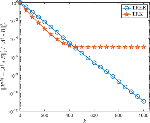
Figure 1: The relative error versus the number of iterations of the TREK and TRK algorithms for a tensor least squares problem.

5.2 Sparse tensor recovery

We compare the performance of the RREK algorithm (Algorithm 3) and the RRK algorithm [7, Algorithm 3.2] for solving the sparse tensor recovery problem (26).

In our experiment, we generate the sensing tensor $\mathcal{A}$, the ground truth tensor $\mathcal{X}_{\rm s}$, and the acquired measurement tensor $\mathcal{B}$ as follows:

$$\mathcal{A}={\tt randn}(N_{1},N_{2},N_{3}),\quad\mathcal{A}(N_{1}-9:N_{1}-5,:,:)=\mathcal{A}(N_{1}-4:N_{1},:,:),$$

$$\mathcal{X}_{\rm s}={\tt randn}(N_{2},K,N_{3}),\quad\mathcal{X}_{\rm s}=\mathcal{X}_{\rm s}.*(\mathcal{X}_{\rm s}>=2.33),$$

$${\mathbf{Z}}={\tt null(bcirc}(\mathcal{A})^{\top}),\quad q={\tt size}(\mathbf{Z},2),\quad\mathcal{B}=\mathcal{A}*\mathcal{X}_{\rm s}+{\tt fold}(\mathbf{Z}*{\tt randn}(q,K))/10.$$

We set $N_{1}=100$, $N_{2}=200$, $N_{3}=10$, and $K=20$. The maximum number of iterations M is 20000. We use the stepsizes $\alpha_{\rm r}=1.5/\lambda_{\rm r}$ and $\alpha_{\rm c}=1.5/\lambda_{\rm c}$. The ground truth $\mathcal{X}_{\rm s}$ is a sparse nonnegative tensor with approximately density $0.01$ and smallest nonzero entry 2.33. In Figure 2, we plot the relative error versus the number of iterations. We observe (i) that the RRK algorithm converges linearly to within a radius of the ground truth $\mathcal{X}_{\rm s}$ and (ii) that the RREK algorithm converges linearly to the ground truth $\mathcal{X}_{\rm s}$.

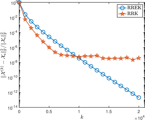
Figure 2: The relative error versus the number of iterations of the RREK and RRK algorithms for a sparse tensor recovery problem.

6 Concluding remarks

We have proposed a randomized regularized extended Kaczmarz algorithm for solving the tensor recovery problem (2). At each step, only one horizontal slice and one lateral slice of the sensing tensor $\mathcal{A}$ are used. Linear convergence of the proposed algorithm is proved under certain assumptions. Numerical experiments on a tensor least squares problem and a sparse tensor recovery problem confirm the theoretical results. In the future, we will use the existing acceleration strategies such as those in [25, 9, 4, 31] to further improve the efficiency when applied to large scale problems. Moreover, we note that the tensor recovery model (2) can be used as a variable selection procedure and we are studying its performance compared with the elastic net [34] and the lasso [30].

References

- [1] Zhong-Zhi Bai and Wen-Ting Wu. On greedy randomized Kaczmarz method for solving large sparse linear systems. SIAM J. Sci. Comput., 40(1):A592–A606, 2018.
- [2] Zhong-Zhi Bai and Wen-Ting Wu. On greedy randomized coordinate descent methods for solving large linear least-squares problems. Numer. Linear Algebra Appl., 26(4):e2237, 15, 2019.
- [3] Zhong-Zhi Bai and Wen-Ting Wu. On partially randomized extended Kaczmarz method for solving large sparse overdetermined inconsistent linear systems. Linear Algebra Appl., 578:225–250, 2019.
- [4] Zhong-Zhi Bai and Wen-Ting Wu. On Greedy Randomized Augmented Kaczmarz Method for Solving Large Sparse Inconsistent Linear Systems. SIAM J. Sci. Comput., 43(6):A3892–A3911, 2021.
- [5] Amir Beck. First-order methods in optimization, volume 25 of MOS-SIAM Series on Optimization. Society for Industrial and Applied Mathematics (SIAM), Philadelphia, PA; Mathematical Optimization Society, Philadelphia, PA, 2017.
- [6] Jian-Feng Cai, Stanley Osher, and Zuowei Shen. Convergence of the linearized Bregman iteration for -norm minimization. Math. Comp., 78(268):2127–2136, 2009.
- [7] Xuemei Chen and Jing Qin. Regularized Kaczmarz algorithms for tensor recovery. SIAM J. Imaging Sci., 14(4):1439–1471, 2021.
- [8] Kui Du. Tight upper bounds for the convergence of the randomized extended Kaczmarz and Gauss–Seidel algorithms. Numer. Linear Algebra Appl., 26(3):e2233, 14, 2019.
- [9] Kui Du, Wu-Tao Si, and Xiao-Hui Sun. Randomized extended average block Kaczmarz for solving least squares. SIAM J. Sci. Comput., 42(6):A3541–A3559, 2020.
- [10] Robert M. Gower and Peter Richtárik. Randomized iterative methods for linear systems. SIAM J. Matrix Anal. Appl., 36(4):1660–1690, 2015.
- [11] Xiang-Long Jiang, Ke Zhang, and Jun-Feng Yin. Randomized block Kaczmarz methods with -means clustering for solving large linear systems. J. Comput. Appl. Math., 403:Paper No. 113828, 14, 2022.
- [12] Stefan Kaczmarz. Angenäherte auflösung von systemen linearer gleichungen. Bull. Intern. Acad. Polonaise Sci. Lett., Cl. Sci. Math. Nat. A, 35:355–357, 1937.
- [13] Misha E. Kilmer, Karen Braman, Ning Hao, and Randy C. Hoover. Third-order tensors as operators on matrices: a theoretical and computational framework with applications in imaging. SIAM J. Matrix Anal. Appl., 34(1):148–172, 2013.
- [14] Misha E. Kilmer and Carla D. Martin. Factorization strategies for third-order tensors. Linear Algebra Appl., 435(3):641–658, 2011.
- [15] Ming-Jun Lai and Wotao Yin. Augmented and nuclear-norm models with a globally linearly convergent algorithm. SIAM J. Imaging Sci., 6(2):1059–1091, 2013.
- [16] Dennis J. Leventhal and Adrian S. Lewis. Randomized methods for linear constraints: convergence rates and conditioning. Math. Oper. Res., 35(3):641–654, 2010.
- [17] Dirk A. Lorenz, Frank Schöpfer, and Stephan Wenger. The linearized Bregman method via split feasibility problems: analysis and generalizations. SIAM J. Imaging Sci., 7(2):1237–1262, 2014.
- [18] Canyi Lu. Tensor-Tensor Product Toolbox. Carnegie Mellon University, June 2018. https://github.com/canyilu/tproduct.
- [19] Anna Ma and Denali Molitor. Randomized Kaczmarz for tensor linear systems. BIT, to appear, 2021.
- [20] Anna Ma, Deanna Needell, and Aaditya Ramdas. Convergence properties of the randomized extended Gauss–Seidel and Kaczmarz methods. SIAM J. Matrix Anal. Appl., 36(4):1590–1604, 2015.
- [21] Yun Miao, Liqun Qi, and Yimin Wei. Generalized tensor function via the tensor singular value decomposition based on the T-product. Linear Algebra Appl., 590:258–303, 2020.
- [22] Ion Necoara. Faster randomized block Kaczmarz algorithms. SIAM J. Matrix Anal. Appl., 40(4):1425–1452, 2019.
- [23] Deanna Needell. Randomized Kaczmarz solver for noisy linear systems. BIT, 50(2):395–403, 2010.
- [24] Deanna Needell and Joel A. Tropp. Paved with good intentions: analysis of a randomized block Kaczmarz method. Linear Algebra Appl., 441:199–221, 2014.
- [25] Deanna Needell, Ran Zhao, and Anastasios Zouzias. Randomized block Kaczmarz method with projection for solving least squares. Linear Algebra Appl., 484:322–343, 2015.
- [26] R. Tyrrell Rockafellar. Convex analysis. Princeton Mathematical Series, No. 28. Princeton University Press, Princeton, N.J., 1970.
- [27] Frank Schöpfer. Linear convergence of descent methods for the unconstrained minimization of restricted strongly convex functions. SIAM J. Optim., 26(3):1883–1911, 2016.
- [28] Frank Schöpfer and Dirk A. Lorenz. Linear convergence of the randomized sparse Kaczmarz method. Math. Program., 173(1-2, Ser. A):509–536, 2019.
- [29] Thomas Strohmer and Roman Vershynin. A randomized Kaczmarz algorithm with exponential convergence. J. Fourier Anal. Appl., 15(2):262–278, 2009.
- [30] Robert Tibshirani. Regression shrinkage and selection via the lasso. J. Roy. Statist. Soc. Ser. B, 58(1):267–288, 1996.
- [31] Wen-Ting Wu. On two-subspace randomized extended Kaczmarz method for solving large linear least-squares problems. Numer. Algorithms, to appear, 2021.
- [32] Yanjun Zhang and Hanyu Li. Block sampling Kaczmarz-Motzkin methods for consistent linear systems. Calcolo, 58(3):Paper No. 39, 20, 2021.
- [33] Yanjun Zhang and Hanyu Li. Greedy Motzkin–Kaczmarz methods for solving linear systems. Numer. Linear Algebra Appl., to appear, 2021.
- [34] Hui Zou and Trevor Hastie. Regularization and variable selection via the elastic net. J. R. Stat. Soc. Ser. B Stat. Methodol., 67(2):301–320, 2005.
- [35] Anastasios Zouzias and Nikolaos M. Freris. Randomized extended Kaczmarz for solving least squares. SIAM J. Matrix Anal. Appl., 34(2):773–793, 2013.