On Generalization and Computation of Tukey’s Depth: Part I

Abstract

Tukey’s depth offers a powerful tool for nonparametric inference and estimation, but also encounters serious computational and methodological difficulties in modern statistical data analysis. This paper studies how to generalize and compute Tukey-type depths in multi-dimensions. A general framework of influence-driven polished subspace depth, which emphasizes the importance of the underlying influence space and discrepancy measure, is introduced. The new matrix formulation enables us to utilize state-of-the-art optimization techniques to develop scalable algorithms with implementation ease and guaranteed fast convergence. In particular, half-space depth as well as regression depth can now be computed much faster than previously possible, with the support from extensive experiments. A companion paper is also offered to the reader in the same issue of this journal.

Keywords: Tukeyfication, estimating equations, projected cone depth, polished subspace depth, Procrustes rotation, Nesterov’s acceleration, nonparametric inference.

1 Introduction

Assessing the uncertainty and reliability of a point or an event of interest is an important but challenging task in many statistical and machine learning applications. Traditional approaches often assume a specific distribution, or rely on asymptotic theory that requires a large sample size relative to the problem dimension, which, in the big-data era, may not meet the challenges of high dimensionality or be too rigid to accommodate various data imperfections. We would like to make the inference data-based and method-driven so that it can apply to any dataset and any estimator. Notably, the method here may refer to an optimization criterion, a set of estimating equations, or a convergent algorithm. It turns out that the concept of data depth offers a universal nonasymptotic tool for robust estimation and inference without having to specify a parametric density.

In 1975, John W. Tukey initiated the idea of location depth (or half-space depth) and demonstrated its use in ranking multivariate data (Tukey,, 1975). Since then, a rich body of literature on depth-based statistical methods has emerged. Though conceptually simple, the powerful idea extends to regression and more general setups (Rousseeuw and Hubert,, 1999; Zhang,, 2002; Mizera,, 2002; Mizera and Müller,, 2004; Müller,, 2005; Zuo,, 2021). In particular, Zhang, (2002) studied a general class of score-function-based location depth and dispersion depth, and Mizera, (2002) pointed out that half-space depth can be criterion-driven, and proposed an operational tangent depth framework when the criterion is differentiable. There also exist many other definitions of data depth, simplicial depth (Liu,, 1990), angular Tukey’s depth (Liu and Singh,, 1992), zonoid depth (Koshevoy and Mosler,, 1997), spatial depth (Vardi and Zhang,, 2000) and projection depth (Zuo,, 2003), to name a few. Data depth provides useful tools in quality control (Liu and Singh,, 1993), hypothesis testing (Yeh and Singh,, 1997; Liu et al.,, 1999; Li and Liu,, 2004), outlier detection (Becker and Gather,, 1999), data visualization (Rousseeuw et al.,, 1999; Buttarazzi et al.,, 2018) and classification (Li et al.,, 2012; Lange et al.,, 2014; Paindaveine and Van Bever,, 2015; Dutta et al.,, 2016). Despite the nice theoretical properties (Nolan,, 1992; He and Wang,, 1997; Nolan,, 1999; Bai and He,, 1999; Zuo and Serfling,, 2000; Chen et al.,, 2018; Gao,, 2020), Tukey-type depths suffer some serious issues that hinder their usage in real-life multivariate data.

Perhaps the biggest challenge lies in computation. Johnson and Preparata, (1978) showed that computing a given point’s location depth is equivalent to solving the closed hemisphere problem, thereby NP-hard. Numerous methods have been developed to compute the exact depth in low dimensions (Ruts and Rousseeuw,, 1996; Rousseeuw and Struyf,, 1998; Aloupis et al.,, 2002; Miller et al.,, 2003) and they are mainly based on enumeration or search. Liu and Zuo, (2014) and Dyckerhoff and Mozharovskyi, (2016) proposed more general algorithms with time complexity $\mathcal{O}(n^{m-1}\log n)$, where $n$ is the sample size and $m$ is the dimensionality. Similarly, multivariate-quantile-based algorithms, Hallin et al., (2010), Kong and Mizera, (2012), Paindaveine and Šiman, (2012), have algorithmic complexity exponentially large in $m$. The computation of an estimate of maximum depth is even more challenging, and interested readers may refer to Rousseeuw and Ruts, (1998), Langerman and Steiger, 2003b , Langerman and Steiger, 2003a and Chan, (2004) among others. In higher dimensions, the class of approximate methods are more affordable and attractive (Rousseeuw and Struyf,, 1998; Dyckerhoff,, 2004; Afshani and Chan,, 2009; Chen et al.,, 2013). They often perform random sampling and projection to reduce the problem to a lower-dimensional one, but the required number of random subsets or projections is still combinatorially large. In experience, even for problems in moderate dimensions, existing packages may either have poor accuracy or incur prohibitive computational costs. We refer to Zuo, (2019) and Shao and Zuo, (2020) for some recent developments.

Moreover, in recent years, researchers have realized some severe scope limitations of Tukey-type depths. For example, for multimodal distributions or those with nonconvex density contours, some definitions of local depth might be more helpful; see Agostinelli and Romanazzi, (2011) and Paindaveine and Van Bever, (2013). Furthermore, modern optimization problems are often defined in a restricted parameter space which may be curved, possess a low intrinsic dimension, or even contain boundaries. Another important class of problems emerging from high-dimensional statistics have nondifferentiable objectives due to the use of regularizers. Examples include variable selection, low-rank matrix estimation, and so on. In such contexts, how to introduce data depth is nontrivial, and has not been systematically studied before in the literature.

This work investigates and extends Tukey’s depth from a subspace learning viewpoint to overcome the aforementioned issues. We aim at operational data depths with efficient computation in multi-dimensions to advance the practice, and hence, abstract concepts for pure theoretical purposes are not the focus. Our main contributions are threefold. (i) A general framework of problem-driven polished subspace depth, which emphasizes the roles of the underlying influence space and discrepancy measure, is presented. (ii) A new matrix formulation enables us to utilize state-of-the-art optimization techniques including majorization-minimization, iterative Procrustes rotations, and Nesterov’s momentum-based acceleration to develop efficient algorithms for depth computation with guaranteed fast convergence. (iii) Two approaches based on manifolds and slack variables extend the notion of depth significantly to accommodate restricted parameter spaces and non-smooth objectives in possibly high dimensions.

In the first part of the work, Section 2 introduces the “Tukeyfication” process in detail and shows how Tukey’s idea can be extended to define influence-driven polished subspace depth. We also study its invariance and give some illustrative examples. Section 3 studies optimization-based depth computation that scales up with problem dimensions and enjoys a sound convergence guarantee. Section 4 performs extensive computer experiments. Some technical details and algorithmic details are left to the appendices. The second part of the work is presented in our companion paper (She et al.,, 2022), which investigates further extensions via manifolds and slack variables to more sophisticated problems.

Notation.

We use bold symbols to denote vectors and matrices. A matrix $\boldsymbol{X}\in\mathbb{R}^{n\times p}$ is frequently partitioned into rows $\boldsymbol{X}=[\boldsymbol{x}_{1}\ldots\boldsymbol{x}_{n}]^{T}$ with $\boldsymbol{x}_{i}\in\mathbb{R}^{p}$. The vectorization of $\boldsymbol{X}$ is denoted by $\textrm{vec}(\boldsymbol{X})\in\mathbb{R}^{np}$. Let $\mathbb{R}_{+}=[0,+\infty]$. Given $\boldsymbol{X}\in\mathbb{R}^{n\times p}$, $\lVert\boldsymbol{X}\rVert_{F}$ and $\lVert\boldsymbol{X}\rVert_{2}$ denote its Frobenius norm and spectral norm, respectively, $\|\boldsymbol{X}\|_{\max}\triangleq\max_{1\leq i\leq n,1\leq j\leq p}|x_{ij}|$, and $\mbox{rank}(\boldsymbol{X})$ denotes its rank. The Moore-Penrose inverse of $\boldsymbol{X}$ is denoted by $\boldsymbol{X}^{+}$. The inner product of two matrices $\boldsymbol{X}$ and $\boldsymbol{Y}$ (of the same size) is defined as $\langle\boldsymbol{X},\boldsymbol{Y}\rangle=\textrm{Tr}(\boldsymbol{X}^{T}\boldsymbol{Y})$ and their element-wise product (Hadamard product) is $\boldsymbol{X}\circ\boldsymbol{Y}$. The Kronecker product is denoted by $\boldsymbol{X}\otimes\boldsymbol{Y}$ (where $\boldsymbol{X}$ and $\boldsymbol{Y}$ need not have the same dimensions). Given a set $\mathcal{A}\subset\mathbb{R}^{p\times m}$ and a matrix $\boldsymbol{T}\in\mathbb{R}^{n\times p}$, $\boldsymbol{T}\circ\mathcal{A}=\{\boldsymbol{T}\boldsymbol{A}:\boldsymbol{A}\in\mathcal{A}\}$. We use $\mathbb{O}^{m\times r}$ to represent the set of all $m\times r$ matrices $\boldsymbol{V}$ satisfying the orthogonality constraint $\boldsymbol{V}^{T}\boldsymbol{V}=\boldsymbol{I}$. For a vector $\boldsymbol{a}=[a_{1},\ldots,a_{n}]^{T}$ $\in\mathbb{R}^{n}$, $\mbox{diag}\{\boldsymbol{a}\}$ is defined as an $n\times n$ diagonal matrix with diagonal entries given by $a_{1},\ldots,a_{n}$, and for a square matrix $\boldsymbol{A}=[a_{ij}]_{n\times n}$, $\mbox{diag}(\boldsymbol{A}):=\mbox{diag}\{a_{11},\ldots,a_{nn}\}$. The indicator function $1_{\mathcal{A}}(t)$ means $1_{\mathcal{A}}(t)=1$ if $t\in\mathcal{A}$ and $0$ otherwise. Given $f:\mathbb{R}^{n\times p}\rightarrow\mathbb{R}$, $f\in\mathcal{C}^{1}$ means that its Euclidean gradient $\nabla f(\boldsymbol{X})$, an $n\times p$ matrix with the $(i,j)$ element ${\partial f}/{\partial x_{ij}}$, exists and is continuous for any $\boldsymbol{X}\in\mathbb{R}^{n\times p}$. Given two vectors $\boldsymbol{\alpha},\boldsymbol{\beta}\in\mathbb{R}^{p}$, $\boldsymbol{\alpha}\succeq\boldsymbol{\beta}$ means $\alpha_{j}\geq\beta_{j},1\leq j\leq p$ and $\boldsymbol{\alpha}\succ\boldsymbol{\beta}$ means $\alpha_{j}>\beta_{j},1\leq j\leq p$.

2 Half-space Depth and Tukeyfication

This section reviews half-space depth and extends it to polished subspace depth, which comprises three key elements: influence function, influence space constraint, and discrepancy measure.

2.1 Three elements for the polished half-space depth

We begin with a close examination of half-space depth. Given $n$ observations $\boldsymbol{z}_{i}\in\mathbb{R}^{m}$, and $\boldsymbol{\mu}^{\circ}$, a location of interest, Tukey’s location or empirical half-space depth is the minimum number of sample points enclosed by a half-space containing $\boldsymbol{\mu}^{\circ}$: $d(\boldsymbol{\mu}^{\circ})=\min_{H\in\mathcal{H}(\boldsymbol{\mu}^{\circ})}{\#}\{i:\boldsymbol{z}_{i}\in H\},$ where $\mathcal{H}(\boldsymbol{\mu}^{\circ})$ is the set of all (closed) half-spaces that cover $\boldsymbol{\mu}^{\circ}$. (The conventional definition refers to $d(\boldsymbol{\mu}^{\circ})/n$, but since we study data depth associated with $n$ observations, all trivial multiplicative factors and additive constants are dropped for simplicity unless otherwise specified.) Motivated by Section 1, a pressing question is to extend this nonparametric tool to any given estimation method.

Below, we work in a supervised setup with $n$ (approximately) i.i.d. observations of $m$ response variables and $p$ predictor variables $(\boldsymbol{y}_{i},\boldsymbol{x}_{i})\in{\mathcal{S}}\subset\mathbb{R}^{m}\times\mathbb{R}^{p}$ ($1\leq i\leq n$), and $\mathcal{S}$ is referred to as the ambient sample space. In the special case of $m$-dimensional location estimation, where there are only observations $\boldsymbol{y}_{i}$ available but no nontrivial predictor variables (i.e., $x_{i}=1$, $1\leq i\leq n$), the sample space is characterized by $\boldsymbol{y}_{i}\in\mathcal{S}\subset\mathbb{R}^{m}$ by convention.

Let $\boldsymbol{X}=[\boldsymbol{x}_{1}\ldots\boldsymbol{x}_{n}]^{T}\in\mathbb{R}^{n\times p}$, $\boldsymbol{Y}=[\boldsymbol{y}_{1}\ldots\boldsymbol{y}_{n}]^{T}\in\mathbb{R}^{n\times m}$, and $\boldsymbol{B}$ be the unknown parameter matrix to estimate. Suppose that the estimation method is specified by a set of estimating equations:

$$\sum_{i=1}^{n}\boldsymbol{T}({\boldsymbol{B}};\boldsymbol{x}_{i},\boldsymbol{y}_{i})=\boldsymbol{0}.$$ (1)

Eqn. (1) can be derived from an optimization problem $\min_{\boldsymbol{B}}f(\boldsymbol{B};\boldsymbol{X},\boldsymbol{Y})$, which is often our starting point in this paper. For example, assuming

$$f(\boldsymbol{B};\boldsymbol{X},\boldsymbol{Y})=\sum_{i}l(\boldsymbol{B};\boldsymbol{x}_{i},\boldsymbol{y}_{i}),$$ (2)

with the same loss $l\in\mathcal{C}^{1}$ (which need not be a negative likelihood function) applied and summed on $n$ approximately i.i.d. sample points, we get $\boldsymbol{T}(\boldsymbol{B};\boldsymbol{x}_{i},\boldsymbol{y}_{i})=\nabla_{\boldsymbol{B}}l(\boldsymbol{B};\boldsymbol{x}_{i},\boldsymbol{y}_{i})$. However, in the presence of a regularizer added in the criterion, the associated estimation equations may not always have the pleasant sample-additive form (She et al.,, 2022).

As pointed out by Peter Rousseeuw and anonymous reviewers, in the above setup, $\boldsymbol{T}(\cdot)$ is proportional to the influence function (Hampel et al.,, 2005), and so we call $\boldsymbol{T}(\boldsymbol{B};\boldsymbol{x}_{i},\boldsymbol{y}_{i})$ (or ${\boldsymbol{T}}_{i}(\boldsymbol{B})$, for short) the influence at observation $i$. We further assume that ${\boldsymbol{T}}_{i}(\boldsymbol{B})$ is in an influence space ${\mathcal{G}}\subset\mathbb{R}^{p\times m}$. Of course, in many applications one can directly define the influences or estimating equations without involving an explicit objective, sometimes from an iterative algorithm or a surrogate function.

Let $\boldsymbol{B}^{\circ}$ be any given point in the parameter space $\Omega\subset\mathbb{R}^{p\times m}$ and $\boldsymbol{T}_{i}^{\circ}=\boldsymbol{T}(\boldsymbol{B}^{\circ};\boldsymbol{x}_{i},\boldsymbol{y}_{i})$. Mimicking Tukey’s location depth, we first project the influences onto a line with direction $\boldsymbol{V}$, and then measure how the estimating equations are maintained via a discrepancy function $\varphi$. This results in the following polished half-space depth (PHD)

$$\mbox{{PHD:}}\quad d_{\varphi}(\boldsymbol{B}^{\circ})=\min_{\boldsymbol{V}}\sum_{i}\varphi(\langle\boldsymbol{V},\boldsymbol{T}_{i}^{\circ}\rangle)\;\textrm{s.t.}\;\lVert\boldsymbol{V}\rVert_{F}=1,\boldsymbol{V}\in\bar{\mathcal{G}},$$ (3)

where $\boldsymbol{V}$ is restricted in a projection space $\bar{\mathcal{G}}$. We call (3) “polished”, owing to (i) the flexibility of $\varphi$, which need not be a monotone function in particular, and (ii) the additional requirement $\boldsymbol{V}\in\bar{\mathcal{G}}$, to complete the notion of depth necessary for defining, for example, covariance depth and Riemannian manifold depth. Although $\bar{\mathcal{G}}$ can be much more general, we set $\bar{\mathcal{G}}=\mathcal{G}$ throughout the work, and the corresponding influence space constraint $\boldsymbol{V}\in\mathcal{G}$ is perhaps natural seen from the inner product $\langle\boldsymbol{V},\boldsymbol{T}_{i}^{\circ}\rangle$. We occasionally write $d_{\varphi}(\boldsymbol{B}^{\circ};\{\boldsymbol{T}_{i}^{\circ}\},\mathcal{G})$ to emphasize its dependence on $\{\boldsymbol{T}_{i}^{\circ}\}$ and $\mathcal{G}$. For more discussions of the inner product, projection, and constraint, see Section LABEL:subsec:RieDep of She et al., (2022) for a general “directional directive” or “geodesic” framework. For supervised problems, a trace form amenable to matrix optimization will be introduced in Section 3. Also, the criterion in (3) can be extended to a U-statistic form.

Special case: when $\varphi(t)=1_{\geq 0}(t)$, we abbreviate $d_{\varphi}$ as $d_{01}$. (Although $1_{\geq 0}$ is conventionally used, $0.5\cdot 1_{=0}+1_{>0}$ is perhaps a better choice for defining $d_{01}$ (She et al.,, 2022), and is more convenient in the successive optimization in Section 3.) Consider a Gaussian location estimation problem that defines the loss of the unknown location ${\boldsymbol{\mu}}\in\Omega=\mathbb{R}^{m}$ as $l(\boldsymbol{\mu};\boldsymbol{z}_{i})=\|\boldsymbol{\mu}-\boldsymbol{z}_{i}\|_{2}^{2}/2$, for $n$ observations $\boldsymbol{z}_{i}\in\mathcal{S}=\mathbb{R}^{m}$, then, $\boldsymbol{T}(\boldsymbol{\mu}^{\circ};\boldsymbol{z}_{i})=\nabla l({\boldsymbol{\mu}};\boldsymbol{z}_{i})|_{{\boldsymbol{\mu}}={\boldsymbol{\mu}}^{\circ}}=\boldsymbol{\mu}^{\circ}-\boldsymbol{z}_{i}\in\mathcal{G}=\mathbb{R}^{m}$, and so $d_{01}$ based on (3) becomes Tukey’s location depth. Similarly, for the ordinary single-response regression, where $m=1$ and the loss is quadratic: $l(\boldsymbol{\beta};\boldsymbol{x}_{i},y_{i})=(\boldsymbol{x}_{i}^{T}\boldsymbol{\beta}-y_{i})^{2}/2$, simple calculation shows $\boldsymbol{T}(\boldsymbol{\beta}^{\circ};\boldsymbol{x}_{i},{y}_{i})=(\boldsymbol{x}_{i}^{T}\boldsymbol{\beta}^{\circ}-{y}_{i})\boldsymbol{x}_{i}$, corresponding to the celebrated regression depth (Rousseeuw and Hubert,, 1999). The sample additive form of the objective in (3) makes it possible to define a population version with respect to a certain distribution $F$, in place of the empirical distribution, but we focus on the sample version without assuming a distribution for the data or an infinite sample size.

The three essential elements in defining (3), namely, $\boldsymbol{T}_{i}^{\circ}$, $\varphi$, and $\mathcal{G}$, deserve a more careful discussion. The influence at observation $i$, not always taking the plain difference $\boldsymbol{\mu}^{\circ}-\boldsymbol{z}_{i}$ as in location depth, can be derived from any criterion. So the influences may be rooted in a parametric model (such as a Gaussian one), but Tukey’s mechanism, which we will refer to as “Tukeyfication”, offers nonparametricness and robustness. In this sense, (3) shares similarities with Owen’s empirical likelihood (Owen,, 2001) which also operates on a given set of estimating equations for nonparametric inference, but can be more robust—for instance, $d_{01}$ targets “Tukey’s median” (far more robust than the $\ell_{1}$-median), instead of the “mean” under (1) or maximum likelihood estimation. However, when the problem under consideration has nondifferentiability or additional constraints, which is common in high-dimensional statistics and machine learning, the influences must be adjusted, which will be examined in our companion paper (She et al.,, 2022).

The influence space $\mathcal{G}$ is often a linear subspace. Under (2), when $\mathcal{G}$ is trivially $\mathbb{R}^{p\times m}$ and $l$ is differentiable, the influence space constraint in (3) is inactive and $d_{01}$ is in the framework of tangent depth (Mizera,, 2002). In general, however, the role of $\mathcal{G}$ cannot be ignored especially in some matrix problems, covariance estimation, multivariate meta analysis and manifold-restricted learning, among others, which gives an important distinction from many depth definitions. We feel that it is necessary to differentiate the sample space, parameter space, and influence space in studying the concept of data depth. The three spaces need not be identical, although for Tukey’s location depth, $\mathcal{S}=\Omega=\mathcal{G}=\mathbb{R}^{m}$. But when $\mathcal{G}$ is not simply the full Euclidean space, one may want to impose some more structural properties on $\boldsymbol{V}$.

With regards to the necessity and benefit of introducing $\varphi$, we notice that the $0$-$1$ loss, though scale free, penalizes projected influences with a constant cost and thus suffers some issues. Specifically, it is non-smooth, the magnitude information of the influences is not taken into account, and the dichotomous measurement may be crude and unstable for influences near zero. To see what other forms $\varphi$ can take, let us assume $\mathcal{G}=\mathbb{R}^{p\times m}$ and rewrite the original half-space depth $d_{01}$ to gain more insights:

$$d_{01}(\boldsymbol{B}^{\circ})=\min_{\lVert\boldsymbol{V}\rVert_{F}=1}\sum 1_{\geq 0}(\langle\boldsymbol{V},\boldsymbol{T}_{i}^{\circ}\rangle)=\min_{\lVert\boldsymbol{V}\rVert_{F}=1}\sum 1_{\leq 0}(\langle\boldsymbol{V},\boldsymbol{T}_{i}^{\circ}\rangle).$$ (4)

The latter form studies a binary classification problem on the margins $\langle\boldsymbol{V},\boldsymbol{T}_{i}^{\circ}\rangle$; other classification losses, such as the hinge loss, logistic deviance, and the Savage loss (Masnadi-shirazi and Vasconcelos,, 2009) can be possibly used. The classification viewpoint enables us to borrow some tools in machine learning for nonasymptotic theoretical analysis. Also, seen from the first expression, one can replace the degenerate $1_{\geq 0}(t)$ for a point mass at zero by any distribution function, and choosing a continuous one can bring in some smoothing effect.

Another useful $\varphi$-family is from the “$\psi$-functions” in M-estimation. (In fact, assuming $\boldsymbol{T}(\boldsymbol{\mu}^{\circ};\boldsymbol{z}_{i})=\boldsymbol{\mu}^{\circ}-\boldsymbol{z}_{i}$ in the location setup, $d_{\psi}$ defined in (3) is the unscaled generalized Tukey depth due to Zhang, (2002); see (12) for our new proposal for handling the scale issue.) Our motivation is from the “contrast” representation of (4)

$$d_{01}(\boldsymbol{B}^{\circ})=({n}/{2})+({1}/{2})\min_{\lVert\boldsymbol{V}\rVert_{F}=1,\boldsymbol{V}\in\mathcal{G}}\sum_{i}\operatorname{sgn}(\langle\boldsymbol{V},\boldsymbol{T}_{i}^{\circ}\rangle),$$ (5)

where $\operatorname{sgn}(t)\triangleq 1_{\geq 0}(t)-1_{<0}(t)$ is just the $\psi$-function associated with the $\ell_{1}$-norm loss except that $\operatorname{sgn}(0)=1$. Zhang, (2002) studied some theoretical properties when using a monotone $\psi$ (such as Huber’s $\psi$). Interestingly, it seems that redescending $\psi$-functions that are non-monotone (Hampel et al.,, 2005), and their rectified versions $\max\{0,\psi(t)\}$ in particular, are potentially useful in dealing with data that are not unimodal; see Figure 1 in Section 2.2.

2.2 Polished subspace depth and invariance

The ideas of projection and polishing apply more generally. For example, we can extend Tukey’s straight line projection to a subspace projection to improve outlier resistance. Toward this, introduce vectorized influences

$$\boldsymbol{t}_{i}^{\circ}=\operatorname{\mbox{vec}\,}(\boldsymbol{T}_{i}^{\circ}),$$ (6)

and assume they are in some influence space denoted by $\mathcal{G}$, a subset of $\mathbb{R}^{pm}$, with a slight abuse of notation. Using $K$, a proper cone (Boyd and Vandenberghe,, 2004, page 43) that induces a partial ordering on $\mathbb{R}^{r}$ ($r\leq pm$) to sort the projected influences, we can define a projected cone depth by

$$\min_{\boldsymbol{V}=[\boldsymbol{v}_{1},\ldots,\boldsymbol{v}_{r}]\in\mathbb{R}^{pm\times r}}\sum_{i}1_{K}(\boldsymbol{V}^{T}\boldsymbol{t}_{i}^{\circ})\mbox{ s.t. }\boldsymbol{V}^{T}\boldsymbol{V}=\boldsymbol{I}_{r\times r},\boldsymbol{v}_{s}\in\mathcal{G},1\leq s\leq r.$$ (7)

In the particular case of $K=\mathbb{R}_{+}^{r}$, a smooth ${\varphi}:\mathbb{R}^{r}\rightarrow\mathbb{R}$ in place of $1_{K}$ gives the polished subspace depth (PSD) which includes the polished half-space depth (3) as $r=1$:

$$\mbox{{PSD:}}\quad d_{\varphi,r}(\boldsymbol{B}^{\circ})\ =\quad\begin{split}&\min_{\boldsymbol{V}=[\boldsymbol{v}_{1},\ldots,\boldsymbol{v}_{r}]\in\mathbb{R}^{pm\times r}}\sum_{i}\prod_{s=1}^{r}\varphi(\boldsymbol{v}_{s}^{T}\boldsymbol{t}_{i}^{\circ})\\ &\qquad\ \ \mbox{ s.t. }\boldsymbol{V}^{T}\boldsymbol{V}=\boldsymbol{I}_{r\times r},\boldsymbol{v}_{s}\in\mathcal{G},1\leq s\leq r.\end{split}$$ (8)

When necessary, we also write the depth as $d_{\varphi,r}(\boldsymbol{B}^{\circ};\{\boldsymbol{t}_{i}^{\circ}\},\mathcal{G})$. It is easy to prove that $d_{01,r}$ is non-increasing in $r$.

To measure the errors more precisely, it is necessary to violate $\varphi(t/\sigma)=\varphi(t)$ $\forall\sigma>0$ (for it would mean that when $r=1$, $\varphi(t)$ must be constant as $t>0$ or $t<0$, i.e., a sign-type function though not necessarily symmetric). Then how do we achieve scale invariance? Zhang, (2002) proposed a scaled form to maintain invariance for location depth, where $\mathcal{G}$ is the full Euclidean space and $\sigma(\cdot)$ is a scale-equivariant function

$$\min_{\boldsymbol{v}}\sum_{i}\varphi\left(\frac{\boldsymbol{v}^{T}(\boldsymbol{\mu}^{\circ}-\boldsymbol{z}_{i})}{\sigma(\{\boldsymbol{v}^{T}(\boldsymbol{\mu}^{\circ}-\boldsymbol{z}_{i})\}_{i=1}^{n})}\right)\;\textrm{s.t.}\;\lVert\boldsymbol{v}\rVert_{2}=1.$$ (9)

But (9) is barely operational from an optimization perspective, because $\boldsymbol{v}$ is involved inside $\sigma$, while $\sigma$ may be nonsmooth or even lack an explicit formula. Moreover, how to extend (9) to $r>1$ is unclear. We give a simple but effective modification of (8) as follows.

First, our goal is to study the invariance of a general $\varphi$-depth under some transformations of the (vectorized) influences. For example, it is preferable to maintain the depth value when switching to scaled influences $\boldsymbol{t}_{i}^{\circ}\rightarrow k\boldsymbol{t}_{i}^{\circ}$ for all $k\in\mathbb{R}$, or even affine-transformed influences $\boldsymbol{t}_{i}^{\circ}\rightarrow\boldsymbol{A}\boldsymbol{t}_{i}^{\circ}$ for all nonsingular $\boldsymbol{A}\in\mathbb{R}^{pm\times pm}$. For some related invariance studies in the scenarios of location depth and regression depth, refer to Zuo and Serfling, (2000) and Zuo, (2021).

Let

$$\bar{\boldsymbol{T}}^{\circ}=[\boldsymbol{t}_{1}^{\circ},\ldots,\boldsymbol{t}_{n}^{\circ}]^{T}\in\mathbb{R}^{n\times pm}$$ (10)

be the matrix formed by vectorized influences. We observe that $d_{\varphi,r}$ defined in (8) does enjoy some sort of orthogonal invariance: for all $\varphi$, $r$, and $\mathcal{G}$,

$$d_{\varphi,r}(\boldsymbol{B}^{\circ};\{\boldsymbol{A}\boldsymbol{t}_{i}^{\circ}\},\boldsymbol{A}\circ\mathcal{G})=d_{\varphi,r}(\boldsymbol{B}^{\circ};\{\boldsymbol{t}_{i}^{\circ}\},\mathcal{G}),\quad\forall\boldsymbol{A}\in\mathbb{O}^{pm\times pm}.$$ (11)

In fact, $d_{\varphi,r}(\boldsymbol{B}^{\circ};\{\boldsymbol{t}_{i}^{\circ}\},\mathcal{G})$ can be defined as $\min\langle\boldsymbol{1},\varphi(\bar{\boldsymbol{T}}^{\circ}\boldsymbol{V})\rangle\mbox{ s.t. }\boldsymbol{v}_{s}\in\mathcal{G},\boldsymbol{V}^{T}\boldsymbol{V}\allowbreak=\boldsymbol{I}$ with $\varphi(\bar{\boldsymbol{T}}^{\circ}\boldsymbol{V})=[\varphi(\boldsymbol{V}^{T}\boldsymbol{t}_{1}^{\circ}),\ldots,\varphi(\boldsymbol{V}^{T}\boldsymbol{t}_{n}^{\circ})]^{T}$; substituting $\bar{\boldsymbol{T}}^{\circ}\boldsymbol{A}^{T}$ for $\bar{\boldsymbol{T}}^{\circ}$ and $\boldsymbol{A}\boldsymbol{V}$ for $\boldsymbol{V}$ keeps the problem unchanged.

Motivated by (11), we define an invariant form of polished subspace depth

$$d_{\varphi,r}^{\boldsymbol{C}}(\boldsymbol{B}^{\circ})=\min_{\boldsymbol{V}\in\mathbb{R}^{pm\times r}}\sum_{i}{\varphi}(\boldsymbol{V}^{T}\boldsymbol{t}_{i}^{\circ})\mbox{ s.t. }\boldsymbol{V}^{T}\boldsymbol{C}(\bar{\boldsymbol{T}}^{\circ})\boldsymbol{V}=\boldsymbol{I}_{r\times r},\boldsymbol{v}_{s}\in\mathcal{G},1\leq s\leq r,$$ (12)

where $\boldsymbol{C}(\bar{\boldsymbol{T}}^{\circ})$ is positive semi-definite and affine equivariant in the sense that

$$\boldsymbol{C}(\bar{\boldsymbol{T}}^{\circ}\boldsymbol{A}^{T})=\boldsymbol{A}\boldsymbol{C}(\bar{\boldsymbol{T}}^{\circ})\boldsymbol{A}^{T}$$ (13)

for any nonsingular $\boldsymbol{A}\in\mathbb{R}^{pm\times pm}$, and $\mbox{rank}(\boldsymbol{C}(\bar{\boldsymbol{T}}^{\circ}))\geq r$. Then it can be easily shown that for any $\varphi$, $r$, $\mathcal{G}$,

$$d_{\varphi,r}^{\boldsymbol{C}}(\boldsymbol{B}^{\circ};\{\boldsymbol{A}\boldsymbol{t}_{i}^{\circ}\},\boldsymbol{A}\circ\mathcal{G})=d_{\varphi,r}^{\boldsymbol{C}}(\boldsymbol{B}^{\circ};\{\boldsymbol{t}_{i}^{\circ}\},(\boldsymbol{A}^{T}\boldsymbol{A})\circ\mathcal{G})$$ (14)

for all nonsingular $\boldsymbol{A}\in\mathbb{R}^{pm\times pm}$. Therefore, if $\mathcal{G}$ is a cone satisfying $a\mathcal{G}=\mathcal{G},\forall a>0$, $d_{\varphi,r}^{\boldsymbol{C}}$ has the desired scale invariance: $d_{\varphi,r}^{\boldsymbol{C}}(\boldsymbol{B}^{\circ};\{k\boldsymbol{t}_{i}^{\circ}\},k\mathcal{G})=d_{\varphi,r}^{\boldsymbol{C}}(\boldsymbol{B}^{\circ};\allowbreak\{\boldsymbol{t}_{i}^{\circ}\},\mathcal{G})$ for any $k\in\mathbb{R}$. Moreover, when $\mathcal{G}$ is the full Euclidean space, like in location depth or regression depth, $(\boldsymbol{A}^{T}\boldsymbol{A})\circ\mathcal{G}=\mathcal{G}$ holds for all nonsingular $\boldsymbol{A}\in\mathbb{R}^{pm\times pm}$, and so $d_{\varphi,r}^{\boldsymbol{C}}$ is affine invariant, as (9), but for all $r$.

Another appealing fact of (12) is that compared with the basic form $d_{\varphi,r}$ (cf. (8)), it adds little cost in computation. When $\mathcal{G}$ is Euclidean, one can convert $d_{\varphi,r}^{\boldsymbol{C}}$ to $d_{\varphi,r}$ with a reparametrization $\boldsymbol{V}^{\prime}=\boldsymbol{D}^{\circ}\boldsymbol{V}^{\circ T}\boldsymbol{V}$, where $\boldsymbol{D}^{\circ},\boldsymbol{U}^{\circ}$ are obtained from the spectral decomposition $\boldsymbol{C}(\bar{\boldsymbol{T}}^{\circ})=\boldsymbol{V}^{\circ}(\boldsymbol{D}^{\circ})^{2}\boldsymbol{V}^{\circ T}$. Specifically, we can simply define $d_{\varphi,r}$ on the column space basis $\boldsymbol{U}^{\circ}$ of $\bar{\boldsymbol{T}}^{\circ}$ (consisting of all left singular vectors of the matrix of vectorized influences), which amounts to $d_{\varphi,r}^{\boldsymbol{C}}$ using $\boldsymbol{C}(\bar{\boldsymbol{T}}^{\circ})=(\bar{\boldsymbol{T}}^{\circ})^{T}\boldsymbol{T}^{\circ}$ that obviously satisfies (13). Based on the previous discussion, this normalized version has affine invariance regardless of $\varphi$ in use. Moreover, owing to the orthogonal invariance, we can prove that the optimization problem depends on $\boldsymbol{U}^{\circ}$ through $\boldsymbol{U}^{\circ}\boldsymbol{U}^{\circ T}$, and so the choice of $\boldsymbol{U}^{\circ}$ will not affect our depth.

Finally, we illustrate the role of $\varphi$ in revealing different characteristics of a dataset with Figure 1. The data points, denoted by crosses, are generated according to a Gaussian mixture model, $y_{i}\stackrel{{\scriptstyle}}{{\sim}}0.5\mathcal{N}(-3,1/16)+0.5\mathcal{N}(3,1/4),1\leq i\leq 10$. We tried some “two-sided” $\varphi$’s in the contrast form (5), constructed from the following $\psi$-functions widely adopted in robust statistics (Hampel et al.,, 2005): the sign $\psi(t)=\operatorname{sgn}(t)$ (note however that $\operatorname{sgn}(0)=1$), Huber’s $\psi(t)=t1_{|t|\leq c}+c\operatorname{sgn}(t)1_{|t|>c}$, the truncated sign $\psi(t)=\operatorname{sgn}(t)1_{|t|\leq c}$ and Tukey’s bisquare $\psi(t)=t(1-(t/c)^{2})^{2}1_{|t|\leq c}$, where we set $c=1$ and then scaled all of them to have a range $[-1,1]$. We also tested some “one-sided” $\varphi$’s in (3) defined via $\psi$: $\varphi(t)=\max\{0,\psi(t)\}$, which we call rectified $\psi$’s. The rectified truncated sign is also considered in Agostinelli and Romanazzi, (2011), and is called the slab function. The results for one-sided $\varphi$’s are shown in Figure 1a) and those for two-sided $\varphi$’s are in Figure 1b).

According to the figure, Tukey’s depth can be achieved using the sign or rectified sign and smoothened by a continuous $\varphi$ (like the ones via Huber’s $\psi$). Moreover, the rectified redescending $\psi$’s offer some local depths on the bimodal dataset, which deserves further investigation. How to choose a proper $\varphi$ to discover desired data features, and whether there is a universal recommendation with certain optimality are beyond the scope of the paper, but we will see that introducing $\varphi$-depth greatly assists computation.

(a)

(a) Examples of one-sided $\varphi$ functions (top row) and the corresponding depth values (bottom row, with a factor of $1/n$). Tukey’s depth uses the 0-1 loss or the rectified sgn function (1st column). The depth curve with rectified Huber (2nd column) is a smoothed version of it. In the 3rd column, the rectified truncated sign function, which is non-monotone, is used as $\varphi$ to generate a local depth curve. In the last column, with Tukey’s bisquare function rectified, a similar local depth curve is obtained with the dashed lines labeling some deepest points.

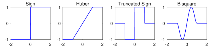
(b)

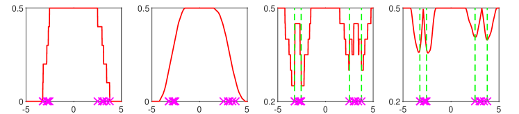
(b) Examples of two-sided $\varphi$ functions (top row) and the corresponding depth values (bottom row, with a factor of $1/n$). 1st column: The sign function leads to the same Tukey’s depth as the one-sided sign. 2nd column: Huber’s $\psi$ smoothes Tukey’s depth, but behaves differently from rectified Huber in (a), say at the points lying outside the support of the data. In the last two columns, redescending functions (without rectification) are used, and some shallowest points that resemble the cluster boundaries are labeled with dashed lines.

Figure 1: An illustration of some $\varphi$ functions (one sided and two sided) and their corresponding depth values on a one-dimensional dataset with the data points denoted by crosses.

2.3 Examples

In the following, we provide some instances in different statistical contexts.

GLM depths

Consider a vector generalized linear model (GLM) with a cumulant function $b$ and the canonical link $g=(b^{\prime})^{-1}$. Then $l(\boldsymbol{B};\boldsymbol{x}_{i},\boldsymbol{y}_{i})=-\langle\boldsymbol{B}^{T}\boldsymbol{x}_{i},\boldsymbol{y}_{i}\rangle+\langle\boldsymbol{1},b(\boldsymbol{B}^{T}\boldsymbol{x}_{i})\rangle$, where $b$ is applied componentwise. The estimation equations are given by

$$\boldsymbol{X}^{T}(b^{\prime}(\boldsymbol{X}\boldsymbol{B})-\boldsymbol{Y})=\boldsymbol{0},$$ (15)

and $\boldsymbol{T}_{i}(\boldsymbol{B})=\boldsymbol{x}_{i}(b^{\prime}(\boldsymbol{B}^{T}\boldsymbol{x}_{i})-\boldsymbol{y}_{i})^{T}\in\mathcal{G}=\mathbb{R}^{p\times m}$, and so (3) becomes

$$d_{\varphi}(\boldsymbol{B}^{\circ})= \min_{\lVert\boldsymbol{V}\rVert_{F}=1}\sum_{i}\varphi(\boldsymbol{x}_{i}^{T}\boldsymbol{V}[b^{\prime}(\boldsymbol{B}^{\circ T}\boldsymbol{x}_{i})-\boldsymbol{y}_{i}])$$ (16)

where $b^{\prime}(\cdot)$ and $\varphi(\cdot)$ are applied element-wise.

First, under the classical Gaussian assumption, $b^{\prime}(\cdot)$ is the identity function, and so (16) covers the multivariate regression depth (Bern and Eppstein,, 2002). How to incorporate dependence into data depth, as raised by Eddy, (1999), is a meaningful question. But under $\boldsymbol{y}_{i}\sim\mathcal{N}(\boldsymbol{B}^{T}\boldsymbol{x}_{i},\boldsymbol{\Sigma})$, the weighted criterion for estimating $\boldsymbol{B}$ is $\mbox{Tr}\{(\boldsymbol{Y}-\boldsymbol{X}\boldsymbol{B})\boldsymbol{\Sigma}^{-1}(\boldsymbol{Y}-\boldsymbol{X}\boldsymbol{B})\}/2$, and thus (15) becomes $\boldsymbol{X}^{T}(\boldsymbol{X}\boldsymbol{B}-\boldsymbol{Y})\boldsymbol{\Sigma}^{-1}=\boldsymbol{0}$ or $\sum\boldsymbol{x}_{i}(\boldsymbol{B}^{T}\boldsymbol{x}_{i}-\boldsymbol{y}_{i})^{T}\boldsymbol{\Sigma}^{-1}=\boldsymbol{0}$. Therefore, adopting an affine invariant depth indicates no need to take the between-response covariance into consideration.

Next, let us consider non-Gaussian GLMs. When $m=1$ and $\varphi(t)=\operatorname{sgn}(t)$, it is well known that the associated GLM depth amounts to applying regression depth on the transformed observations $(g(y_{i}),\boldsymbol{x}_{i})$ owing to the property: $\operatorname{sgn}(\boldsymbol{x}_{i}^{T}\boldsymbol{v}(b^{\prime}(\boldsymbol{x}_{i}^{T}\boldsymbol{\beta})-y_{i}))=\operatorname{sgn}(\langle\boldsymbol{v},\boldsymbol{x}_{i}\rangle)\operatorname{sgn}(u(b^{\prime}(\boldsymbol{x}_{i}^{T}\boldsymbol{\beta}))-u(y_{i}))$ for any strictly increasing $u$ (Van Aelst et al.,, 2002). However, we remark that the monotone invariance property does not hold in general for multivariate problems ($m>1$), and so GLM depths do have their value. We can also use the logistic regression depth to illustrate the weakness of $\varphi(t)=\operatorname{sgn}(t)$. Let $m=1$, $r_{i}=b^{\prime}(\boldsymbol{x}_{i}^{T}\boldsymbol{\beta})-y_{i}=\exp(\boldsymbol{x}_{i}^{T}\boldsymbol{\beta})/(1+\exp(\boldsymbol{x}_{i}^{T}\boldsymbol{\beta}))-y_{i}$. For such binary $y_{i}$, the sigmoidal $r_{i}$ appear more reasonable than the difference-based residuals $\boldsymbol{x}_{i}^{T}\boldsymbol{\beta}-y_{i}$ in regression. But because $\operatorname{sgn}(r_{i})=1-2y_{i}$ (regardless of the difference between $\exp(\boldsymbol{x}_{i}^{T}\boldsymbol{\beta})/(1+\exp(\boldsymbol{x}_{i}^{T}\boldsymbol{\beta}))$ and $y_{i}$), the resulting depth does not vary with $\boldsymbol{\beta}\in\mathbb{R}^{p}$ as long as it is finite, an evidence of the crudeness of $d_{01}$ in this scenario.

Finally, we point out that although one could vectorize (15) via $\boldsymbol{y}=\operatorname{\mbox{vec}\,}(\boldsymbol{Y})\in\mathbb{R}^{nm}$, $\boldsymbol{\beta}=\operatorname{\mbox{vec}\,}(\boldsymbol{B})\in\mathbb{R}^{pm}$ and $\boldsymbol{Z}=\boldsymbol{I}\otimes\boldsymbol{X}$ to get

$$\boldsymbol{Z}^{T}(b^{\prime}(\boldsymbol{Z}\boldsymbol{\beta})-\boldsymbol{y})=\boldsymbol{0},$$ (17)

the associated data depth would not have a valid population definition. In fact, $\boldsymbol{Z}$ has a block diagonal form, meaning that its rows cannot be treated as observations following the same distribution, and the vectorized equations do not have the desired sample additivity on $(\boldsymbol{x}_{i},\boldsymbol{y}_{i})$, $1\leq i\leq n$. Introducing data depth via the generalized estimating equations (GEEs) (Liang and Zeger,, 1986) may suffer the same issue. Concretely, the GEEs for our problem are given by

$$(\boldsymbol{I}\otimes\boldsymbol{X})^{T} \mbox{diag}\{(b^{\prime\prime})^{1/2}(\operatorname{\mbox{vec}\,}(\boldsymbol{X}\boldsymbol{B}))\}\ \times\ \boldsymbol{W}^{-1}\times$$ (18)

$$\mbox{diag}\{(b^{\prime\prime})^{-1/2}(\operatorname{\mbox{vec}\,}(\boldsymbol{X}\boldsymbol{B}))\}(b^{\prime}(\operatorname{\mbox{vec}\,}(\boldsymbol{X}\boldsymbol{B}))-\operatorname{\mbox{vec}\,}(\boldsymbol{Y}))=\boldsymbol{0},$$

where the working correlation matrix $\boldsymbol{W}=\boldsymbol{\Sigma}\otimes\boldsymbol{I}$ with $\boldsymbol{\Sigma}$ known (say, the sample correlation matrix of $\boldsymbol{Y}$ or some regularized estimate). In the special case that $b^{\prime}$ is identity or $\boldsymbol{\Sigma}$ is diagonal, $\{(b^{\prime\prime})^{1/2}(\operatorname{\mbox{vec}\,}(\boldsymbol{X}\boldsymbol{B}^{\circ}))\}$ and $\mbox{diag}\{(b^{\prime\prime})^{-1/2}(\operatorname{\mbox{vec}\,}(\boldsymbol{X}\boldsymbol{B}^{\circ}))\}$ cancel, and (18) can be rephrased as $\boldsymbol{X}^{T}(b^{\prime}(\boldsymbol{X}\boldsymbol{B})-\boldsymbol{Y})\boldsymbol{\Sigma}^{-1}=\boldsymbol{0}$, which is sample additive. But the property holds no longer for multivariate non-Gaussian GEEs to induce a legitimate data depth.

Covariance depth

Assume that $\textrm{vec}(\boldsymbol{Y})\sim\mathcal{N}(\boldsymbol{0},\boldsymbol{\Sigma}\otimes\boldsymbol{I})$ for $\boldsymbol{Y}\in\mathbb{R}^{n\times m}$, where the between-column covariance matrix $\boldsymbol{\Sigma}$ is positive definite. Let $\boldsymbol{W}=\boldsymbol{\Sigma}^{-1}$. From the negative log-likelihood $l(\boldsymbol{W};\boldsymbol{y}_{i})=(\textrm{Tr}(\boldsymbol{W}\boldsymbol{y}_{i}\boldsymbol{y}_{i}^{T})-\log\det\boldsymbol{W})/n$ (up to some scaling and additive constants), we know that its gradient takes a simple difference form $(\boldsymbol{y}_{i}\boldsymbol{y}_{i}^{T}-\boldsymbol{\Sigma})/n$, symmetric but not necessarily positive semi-definite. The depth for a positive definite $\boldsymbol{\Sigma}^{\circ}$ according to (3) is

$$d_{\varphi}(\boldsymbol{\Sigma}^{\circ})=\min_{\boldsymbol{V}}\sum_{i}\varphi(\boldsymbol{y}_{i}^{T}\boldsymbol{V}\boldsymbol{y}_{i}-\langle\boldsymbol{V},\boldsymbol{\Sigma}^{\circ}\rangle),\mbox{ s.t. }\lVert\boldsymbol{V}\rVert_{F}=1,\boldsymbol{V}=\boldsymbol{V}^{T},$$

where $\boldsymbol{V}$ is additionally required to be symmetric, as an outcome of the symmetry of the gradient. Adding a further rank restriction: $\textrm{rank}(\boldsymbol{V})=1$, $\boldsymbol{V}$ simplifies to $\pm\boldsymbol{v}\boldsymbol{v}^{T}$, which leads to

$$d_{\varphi}(\boldsymbol{\Sigma}^{\circ})=\min_{\boldsymbol{v}\in\mathbb{R}^{m},\lVert\boldsymbol{v}\rVert_{2}=1} \sum_{i}\varphi((\boldsymbol{y}_{i}^{T}\boldsymbol{v})^{2}-\boldsymbol{v}^{T}\boldsymbol{\Sigma}^{\circ}\boldsymbol{v})\wedge\sum_{i}\varphi(-(\boldsymbol{y}_{i}^{T}\boldsymbol{v})^{2}+\boldsymbol{v}^{T}\boldsymbol{\Sigma}^{\circ}\boldsymbol{v}),$$

and $\varphi(t)=1_{\geq 0}(t)$ corresponds to the notion of matrix depth in Chen et al., (2018). (The unit-rank reduction to a vector $\boldsymbol{v}$ is however incompatible with imposing elementwise sparsity in covariance estimation; see Section LABEL:subsec:slack of our companion paper for a new idea of how to define sparsity induced depth and deepest $s$-sparse estimators.)

Similarly, we can introduce depth for meta-regression with multiple outcomes. This could be helpful to alleviate the stringent normality assumption in meta-analysis. Assume there are $n$ studies with $\boldsymbol{\Sigma}_{i}$ as the known within-study covariances: $\boldsymbol{y}_{i}=\boldsymbol{X}_{i}\boldsymbol{\beta}+\boldsymbol{\epsilon}_{i}+\boldsymbol{\delta}_{i}$ ($1\leq i\leq n$), where $\boldsymbol{\epsilon}_{i}\sim\mathcal{N}(\boldsymbol{0},\boldsymbol{\Sigma}_{i})$ are independent of $\boldsymbol{\delta}_{i}\sim\mathcal{N}(\boldsymbol{0},\boldsymbol{\Sigma})$. Let $\boldsymbol{R}_{i}=(\boldsymbol{y}_{i}-\boldsymbol{X}_{i}\boldsymbol{\beta})(\boldsymbol{y}_{i}-\boldsymbol{X}_{i}\boldsymbol{\beta})^{T}$. When the between-study covariance $\boldsymbol{\Sigma}$ is of interest and $\boldsymbol{\beta}$ is held fixed, we have $\boldsymbol{T}_{i}(\boldsymbol{\Sigma})=(\boldsymbol{\Sigma}+\boldsymbol{\Sigma}_{i})^{-1}(\boldsymbol{\Sigma}+\boldsymbol{\Sigma}_{i}-\boldsymbol{R}_{i})(\boldsymbol{\Sigma}+\boldsymbol{\Sigma}_{i})^{-1}$, which again results in a symmetric $\mathcal{G}$.

Projected triangle depth

Consider projecting all data points $\boldsymbol{z}_{i}\in\mathbb{R}^{m}$ ($1\leq i\leq n$) to $\mathbb{R}^{2}$ to calculate the simplicial depth (Liu,, 1990). Let $\triangle(\boldsymbol{z}_{i},\boldsymbol{z}_{j},\boldsymbol{z}_{k})$ denote the non-degenerate triangle formed by $\boldsymbol{z}_{i},\boldsymbol{z}_{j},\boldsymbol{z}_{k}$ and assume that the data have been pre-processed to remove any collinearity. Given any $\boldsymbol{V}\in\mathbb{R}^{m\times 2}:\boldsymbol{V}^{T}\boldsymbol{V}=\boldsymbol{I}_{2\times 2}$, denote the projected point of $\boldsymbol{z}$ by ${\mathbf{P}}_{\boldsymbol{V}}(\boldsymbol{z})=\boldsymbol{V}^{T}\boldsymbol{z}\in\mathbb{R}^{2}$ and the augmented point by $\bar{{\mathbf{P}}}_{\boldsymbol{V}}(\boldsymbol{z})=[\boldsymbol{z}^{T}\boldsymbol{V}\;1]^{T}\in\mathbb{R}^{3}$. Define the projected triangle depth for a target point $\boldsymbol{\mu}^{\circ}$ by $d(\boldsymbol{\mu}^{\circ})=\min_{\boldsymbol{V}}\#\{(i,j,k):i<j<k,{\mathbf{P}}_{\boldsymbol{V}}(\boldsymbol{\mu}^{\circ})\in\triangle({\mathbf{P}}_{\boldsymbol{V}}(\boldsymbol{z}_{i}),{\mathbf{P}}_{\boldsymbol{V}}(\boldsymbol{z}_{j}),{\mathbf{P}}_{\boldsymbol{V}}(\boldsymbol{z}_{k}))\}$ s.t. $\boldsymbol{V}\in\mathbb{R}^{m\times 2},\boldsymbol{V}^{T}\boldsymbol{V}=\boldsymbol{I}$, and introduce the $\varphi$-form

$$\min_{\boldsymbol{V}\in\mathbb{R}^{m\times 2}}\sum_{i<j<k}\prod_{l=1}^{3}\varphi(\xi_{l}^{\circ}(\boldsymbol{z}_{i},\boldsymbol{z}_{j},\boldsymbol{z}_{k};\boldsymbol{V}))\;\textrm{s.t.}\;\boldsymbol{V}^{T}\boldsymbol{V}=\boldsymbol{I},$$ (19)

where $\boldsymbol{\xi}^{\circ}=[\xi_{l}^{\circ}]_{l=1}^{3}=[\bar{{\mathbf{P}}}_{\boldsymbol{V}}(\boldsymbol{z}_{i})\;\bar{{\mathbf{P}}}_{\boldsymbol{V}}(\boldsymbol{z}_{j})\;\bar{{\mathbf{P}}}_{\boldsymbol{V}}(\boldsymbol{z}_{k})]^{-1}\bar{{\mathbf{P}}}_{\boldsymbol{V}}(\boldsymbol{\mu}^{\circ})$. Here, we used the fact that ${\mathbf{P}}_{\boldsymbol{V}}(\boldsymbol{\mu}^{\circ})$ belongs to the projected triangle $\triangle({\mathbf{P}}_{\boldsymbol{V}}(\boldsymbol{y}_{i}),{\mathbf{P}}_{\boldsymbol{V}}(\boldsymbol{y}_{j}),{\mathbf{P}}_{\boldsymbol{V}}(\boldsymbol{y}_{k}))$ if and only if $[\bar{{\mathbf{P}}}_{\boldsymbol{V}}(\boldsymbol{z}_{i})\ \ \allowbreak\bar{{\mathbf{P}}}_{\boldsymbol{V}}(z_{j})\ \allowbreak\ \bar{{\mathbf{P}}}_{\boldsymbol{V}}(\boldsymbol{z}_{k})]\boldsymbol{\xi}^{\circ}=\bar{{\mathbf{P}}}_{\boldsymbol{V}}(\boldsymbol{\mu}^{\circ})$ has a nonnegative solution $\boldsymbol{\xi}^{\circ}$. Because $\boldsymbol{\xi}^{\circ}$ is smooth in $\boldsymbol{V}$, the optimization techniques developed in Section 3 apply. A similar formulation can be given for the simplicial depth without projection, and to speed up the computation, one may consider a randomized version as in Afshani and Chan, (2009).

3 Optimization-based Depth Computation

The biggest obstacle to the application of Tukey-type depths is perhaps the heavy computational cost as mentioned in Section 1. Even in moderate dimensions, the available methods often suffer from either prohibitively high computational complexity or poor accuracy. Unlike many existing algorithms and procedures that are designed based on geometry, or try to find smart ways of numeration or search, this section develops optimization based depth computation with a rigorous convergence guarantee. Our ultimate target in this section is $d_{01}$ but we will see that the $\varphi$-form data depth facilitates algorithm design. Before describing the thorough detail, it may help the reader to check Figure 2 for an illustration of the power brought by optimization. Even though the initial half-space is in one of the worst directions, the optimal half-space is found in $10$ iterations. An outline of the associated algorithm is given in Appendix A.

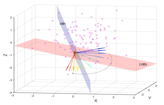
Figure 2: An example of optimization-based depth computation. The initial half-space is in one of the worst directions, but after $10$ steps, the optimal half-space is found.

For clarity, we will mainly use the polished half-space depth to describe the derivation details, although in principle the same algorithm design applies to the polished subspace depth as well. Because the loss in supervised learning is typically placed on the systematic component ${\boldsymbol{\Theta}}=\boldsymbol{X}\boldsymbol{B}$, and we denote by $\bar{l}(\boldsymbol{\Theta};\boldsymbol{Y})=\sum_{i}l_{0}(\boldsymbol{B}^{T}\boldsymbol{x}_{i};\boldsymbol{y}_{i})/n$ the estimation criterion with $\ell_{0}\in\mathcal{C}^{1}$. Then, the depth problem $\min\sum_{i}\varphi(\langle\boldsymbol{V},\boldsymbol{T}_{i}^{\circ}\rangle)\;\textrm{s.t.}\;\lVert\boldsymbol{V}\rVert_{F}=1,\boldsymbol{V}\in\mathcal{G}$ can be restated in a trace form that is perhaps more amenable to matrix optimization:

$$\min_{\boldsymbol{V}\in\mathcal{G},\,\lVert\boldsymbol{V}\rVert_{F}=1}f(\boldsymbol{V})\triangleq\textrm{Tr}\{\varphi(\boldsymbol{X}\boldsymbol{V}\boldsymbol{R}^{T})\},$$ (20)

where $\varphi$ is applied elementwise, i.e., $\varphi(\boldsymbol{X})_{ij}=\varphi(x_{ij})$, and

$$\boldsymbol{R}=\nabla_{\boldsymbol{\Theta}}\bar{l}\,\lvert_{\boldsymbol{\Theta}=\boldsymbol{X}\boldsymbol{B}^{\circ}}.$$

A particular instance is the GLM depth defined in (16), where $\boldsymbol{R}=b^{\prime}(\boldsymbol{X}\boldsymbol{B}^{\circ})-\boldsymbol{Y}$. We can also write $\boldsymbol{R}=[\boldsymbol{r}_{1},\ldots,\boldsymbol{r}_{n}]^{T}$ with $\boldsymbol{r}_{i}=\nabla l_{0}(\operatorname{\mbox{vec}\,}(\boldsymbol{\Theta}[i,]);\boldsymbol{y}_{i})$, and then $f(\boldsymbol{V})=\sum_{i}\varphi(\langle\boldsymbol{V},\boldsymbol{T}_{i}^{\circ}\rangle)$ and $\boldsymbol{T}_{i}^{\circ}=\boldsymbol{x}_{i}\boldsymbol{r}_{i}^{T}$. Formally, given $\boldsymbol{X}^{T}\boldsymbol{R}=\boldsymbol{0}$, where the $i$th row of $\boldsymbol{R}$ depends on the $i$th sample $(\boldsymbol{x}_{i},\boldsymbol{y}_{i})$ only (thereby sample-additive), the associated depth objective is $\textrm{Tr}\{\varphi(\boldsymbol{X}\boldsymbol{V}\boldsymbol{R}^{T})\}$.

Assume that $\varphi$ is continuously differentiable for now. We can develop a prototype algorithm following the principle of majorization-minimization (MM) (Hunter and Lange,, 2004), where a surrogate function needs to be created to majorize the objective so that minimizing this surrogate function drives it downhill. We use a quadratic surrogate function:

$$g_{\rho}(\boldsymbol{V},\boldsymbol{V}^{-})=f(\boldsymbol{V}^{-})+\langle\boldsymbol{X}^{T}(\textrm{diag}(\varphi^{\prime}(\boldsymbol{X}\boldsymbol{V}^{-}\boldsymbol{R}^{T}))\boldsymbol{R},\boldsymbol{V}-\boldsymbol{V}^{-}\rangle+\frac{\rho}{2}\lVert\boldsymbol{V}-\boldsymbol{V}^{-}\rVert_{F}^{2},$$ (21)

where $\rho>0$ and $\mbox{diag}(\boldsymbol{A})$ is a diagonal matrix formed by the diagonal entries of $\boldsymbol{A}$. Here, $\boldsymbol{X}^{T}(\textrm{diag}(\varphi^{\prime}(\boldsymbol{X}\boldsymbol{V}^{-}\boldsymbol{R}^{T}))\boldsymbol{R}$ is the gradient of $f$; in implementation, the diagonal entries of $\boldsymbol{X}\boldsymbol{V}\boldsymbol{R}^{T}$ can be efficiently calculated by the row sums of $(\boldsymbol{X}\boldsymbol{V})\circ\boldsymbol{R}$, where $\circ$ denotes the elementwise product. Starting with $\boldsymbol{V}^{(0)}:\lVert\boldsymbol{V}^{(0)}\rVert_{F}=1$, we define a sequence of $\boldsymbol{V}$-iterates by

$$\boldsymbol{V}^{(t+1)}\in\operatorname*{argmin}_{\boldsymbol{V}\in\mathcal{G},\,\lVert\boldsymbol{V}\rVert_{F}=1}g_{\rho_{t}}(\boldsymbol{V},\boldsymbol{V}^{(t)}),$$ (22)

for any $t\geq 0$. We prove a convergence result for the resulting algorithm assuming $\varphi^{\prime}$ is Lipschitz continuous: $\lvert\varphi^{\prime}(x)-\varphi^{\prime}(y)\rvert\leq L\lvert x-y\rvert$, $\forall x,y\in\mathbb{R}$. Recall that $\|\cdot\|_{2}$ denotes the spectral norm of the enclosed matrix.

Theorem 3.1.

If $\rho_{t}$ is chosen large enough, e.g., $\rho_{t}\geq L\lVert\boldsymbol{X}\rVert_{2}^{2}\lVert\boldsymbol{R}\rVert_{2}^{2}$, then (22) satisfies

$$f(\boldsymbol{V}^{(t+1)})\leq g_{\rho_{t}}(\boldsymbol{V}^{(t+1)},\boldsymbol{V}^{(t)})\leq g_{\rho_{t}}(\boldsymbol{V}^{(t)},\boldsymbol{V}^{(t)})=f(\boldsymbol{V}^{(t)}),\ \forall t\geq 0$$ (23)

That is, the objective function value is guaranteed non-increasing throughout the iteration.

The convergence of the algorithm holds more generally. The Lipschitz parameter is used to derive a universal step-size; in implementation, we recommend performing a line search. Specifically, we can decrease $1/\rho_{t}$ until $f(\boldsymbol{V}^{(t+1)}(\rho_{t}))\leq g_{\rho_{t}}(\boldsymbol{V}^{(t+1)}(\rho_{t}),\boldsymbol{V}^{(t)})$ is satisfied (and so $f(\boldsymbol{V}^{(t+1)})\leq f(\boldsymbol{V}^{(t)})$ still holds for any $t$). The decrease in function value in the pursuit of projection direction offers more stability than geometry or search based algorithms. The surrogate via linearization applies to polished subspace depth as well.

Because $g_{\rho}(\boldsymbol{V},\boldsymbol{V}^{-})=\rho\lVert\boldsymbol{V}-(\boldsymbol{V}^{-}-({1}/{\rho})\boldsymbol{X}^{T}(\textrm{diag}(\varphi^{\prime}(\boldsymbol{X}\boldsymbol{V}^{-}\boldsymbol{R}^{T}))\boldsymbol{R})\rVert_{F}^{2}/2+f(\boldsymbol{V}^{-})-(1/2\rho)\|\boldsymbol{X}^{T}(\textrm{diag}(\varphi^{\prime}(\boldsymbol{X}\boldsymbol{V}^{-}\boldsymbol{R}^{T}))\boldsymbol{R}\|_{F}^{2}$, the problem at each iteration boils down to

$$\min\ \lVert\boldsymbol{V}-(\boldsymbol{V}^{(t)}-\frac{1}{\rho_{t}}\boldsymbol{G}^{(t)})\rVert_{F}^{2}\quad\textrm{s.t.\quad}\lVert\boldsymbol{V}\rVert_{F}=1,\boldsymbol{V}\in\mathcal{G}$$ (24)

where $\boldsymbol{G}^{(t)}=\boldsymbol{X}^{T}(\textrm{diag}(\varphi^{\prime}(\boldsymbol{X}\boldsymbol{V}^{(t)}\boldsymbol{R}^{T}))\boldsymbol{R}$. Eqn. (24) has many variants depending on the projection space constraint. For instance, when solving (8) or (19), the problem after linearization projects to a Stiefel manifold instead of a sphere. Some more examples are given in Appendix B.

We assume that $\mathcal{G}$ is a linear subspace in the rest of the section (which includes the class of Riemannian depth in our companion paper). Then (24) can be converted to a case of Procrustes rotation. Define a linear mapping $\boldsymbol{B}=\mathcal{G}(\boldsymbol{A})$ such that $\operatorname{\mbox{vec}\,}(\boldsymbol{B})=\mathcal{P}_{\mathcal{G}}\operatorname{\mbox{vec}\,}(\boldsymbol{A})$, where $\mathcal{P}_{\mathcal{G}}$ is the orthogonal projection matrix onto subspace $\mathcal{G}$. By writing $\operatorname{\mbox{vec}\,}(\boldsymbol{V}^{(t)}-\boldsymbol{G}^{(t)}/{\rho_{t}})=\mathcal{P}_{\mathcal{G}}\operatorname{\mbox{vec}\,}(\boldsymbol{V}^{(t)}-\boldsymbol{G}^{(t)}/{\rho_{t}})+\mathcal{P}_{\mathcal{G}}^{\perp}\operatorname{\mbox{vec}\,}(\boldsymbol{V}^{(t)}-\boldsymbol{G}^{(t)}/{\rho_{t}})$, we obtain

$$\boldsymbol{V}^{(t+1)}=\mathcal{G}(\boldsymbol{V}^{(t)}-\boldsymbol{G}^{(t)}/{\rho_{t}})/\lVert\mathcal{G}(\boldsymbol{V}^{(t)}-\boldsymbol{G}^{(t)}/{\rho_{t}})\rVert_{F}.$$

Though not a proximity operator due to nonconvexity, the projection guarantees global optimality in solving (24) (cf. Lemma D.1).

Furthermore, we find that Nesterov’s second acceleration for convex programming (Nesterov,, 2004), which attains the optimal convergence rate of $\mathcal{O}(1/t^{2})$ among first-order methods, can be modified to speed the convergence of the prototype algorithm. (Empirically, Nesterov’s first acceleration appears to be also effective, but we cannot provide its theoretical support.) To aid the presentation of the acceleration scheme, we define the generalized Bregman function (She et al.,, 2021) for any continuously differentiable $\psi$

$$\boldsymbol{\Delta}_{\psi}(\boldsymbol{\beta},\boldsymbol{\gamma}):=\psi(\boldsymbol{\beta})-\psi(\boldsymbol{\gamma})-\langle\nabla\psi(\boldsymbol{\gamma}),\boldsymbol{\beta}-\boldsymbol{\gamma}\rangle.$$ (25)

When $\psi$ is strictly convex, $\boldsymbol{\Delta}_{\psi}$ becomes the standard Bregman divergence $\mathbf{D}_{\psi}(\boldsymbol{\beta},\boldsymbol{\gamma})$ (Bregman,, 1967). A simple example is $\mathbf{D}_{2}(\boldsymbol{\beta},\boldsymbol{\gamma}):=\|\boldsymbol{\beta}-\boldsymbol{\gamma}\|_{2}^{2}/2$, where ${\mathbf{D}}_{2}$ denotes the Bregman associated with the half-squared-error-loss function, and its matrix version is ${\mathbf{D}}_{2}(\boldsymbol{A},\boldsymbol{B})=\|\operatorname{\mbox{vec}\,}(\boldsymbol{A})-\operatorname{\mbox{vec}\,}(\boldsymbol{B})\|_{2}^{2}/2=\|\boldsymbol{A}-\boldsymbol{B}\|_{F}^{2}/2$. In general, $\boldsymbol{\Delta}_{\psi}$ or $\mathbf{D}_{\psi}$ may not be symmetric.

Consider the following momentum-based update which involves three major sequences $\boldsymbol{U}^{(t)}$, $\boldsymbol{W}^{(t)}$, $\boldsymbol{V}^{(t)}$, $t=0,1,\ldots$ (starting with $\theta_{0}=1$ and any $\boldsymbol{W}^{(0)}\in\mathbb{R}^{p\times m}$):

$$\boldsymbol{U}^{(t)} =(1-\theta_{t})\boldsymbol{V}^{(t)}+\theta_{t}\boldsymbol{W}^{(t)},$$ (26)

$$\boldsymbol{G}^{(t)} =\boldsymbol{X}^{T}(\textrm{diag}(\varphi^{\prime}(\boldsymbol{X}\boldsymbol{U}^{(t)}\boldsymbol{R}^{T}))\boldsymbol{R},$$ (27)

$$\boldsymbol{\Xi}^{(t)} =\mathcal{G}(\boldsymbol{W}^{(t)}-\boldsymbol{G}^{(t)}/\{\theta_{t}\rho_{t}\}),$$ (28)

$$\boldsymbol{W}^{(t+1)} =\boldsymbol{\Xi}^{(t)}/\|\boldsymbol{\Xi}^{(t)}\|_{F},$$ (29)

$$\boldsymbol{V}^{(t+1)} =(1-\theta_{t})\boldsymbol{V}^{(t)}+\theta_{t}\boldsymbol{W}^{(t+1)}.$$ (30)

The design of the relaxation parameters $\theta_{t}$ and inverse stepsize parameters $\rho_{t}$ holds the key to acceleration. We propose the following line search criterion

$$R_{t}\triangleq\theta_{t}^{2}\rho_{t}\mathbf{D}_{2}(\boldsymbol{W}^{(t+1)},\boldsymbol{W}^{(t)})-\boldsymbol{\Delta}_{f}(\boldsymbol{V}^{(t+1)},\boldsymbol{U}^{(t)})+(1-\theta_{t})\boldsymbol{\Delta}_{f}(\boldsymbol{V}^{(t)},\boldsymbol{U}^{(t)})\geq 0,~{}~{}~{}~{}~{}$$ (31)

$$\frac{\theta_{t}^{2}}{1-\theta_{t}}=\frac{\rho_{t-1}\theta_{t-1}^{2}}{\rho_{t}},~{}\theta_{t}\geq 0,\rho_{t}>0,t\geq 1.$$ (32)

and $\theta_{0}=1$. Some implementation details are given in Algorithm 1. When $f$ has $L$-Lipschitz continuity in its gradient, (31) is implied by

$$\theta_{t}^{2}(\rho_{t}-L)\mathbf{D}_{2}(\boldsymbol{W}^{(t+1)},\boldsymbol{W}^{(t)})+(1-\theta_{t})\boldsymbol{\Delta}_{f}(\boldsymbol{V}^{(t)},\boldsymbol{U}^{(t)})\geq 0.$$ (33)

If, further, $f$ is convex, taking $\rho_{t}=L$ and $\theta_{t+1}=(\sqrt{\theta_{t}^{4}+4\theta_{t}^{2}}-\theta_{t}^{2})/2$ gives the standard convex second acceleration (Tseng,, 2010). The reasonability of (31) in our nonconvex setup can be seen from the following theorem, where the convergence is shown under a proper discrepancy measure.

Theorem 3.2.

Given any $\rho_{t}>0$ ($t\geq 0$), consider the algorithm defined by (26)–(30) and (32). Then for any $\boldsymbol{V}\in\mathcal{G}:\|\boldsymbol{V}\|_{F}=1$ and $T\geq 0$,

$$\begin{split}\frac{f(\boldsymbol{V}^{(T+1)})-f(\boldsymbol{V})}{\theta_{T}^{2}\rho_{T}}+T\cdot\mathop{\mathrm{avg}}_{0\leq t\leq T}\frac{\mathcal{E}_{t}(\boldsymbol{V})}{\theta_{t}\rho_{t}}+T\cdot\mathop{\mathrm{avg}}_{0\leq t\leq T}\frac{R_{t}}{\theta_{t}^{2}\rho_{t}}\\ \leq\mathbf{D}_{2}(\boldsymbol{V},\boldsymbol{W}^{(0)})-\mathbf{D}_{2}(\boldsymbol{V},\boldsymbol{W}^{(T+1)}),\end{split}$$ (34)

where $\mathcal{E}_{t}(\boldsymbol{V})=\boldsymbol{\Delta}_{f}(\boldsymbol{V},\boldsymbol{U}^{(t)})+\theta_{t}\rho_{t}(\|\boldsymbol{\Xi}^{(t)}\|_{F}-1)\mathbf{D}_{2}(\boldsymbol{V},\boldsymbol{W}^{(t+1)})$.

Typically, (31) involves a line search. If the condition fails for the current value of $\rho_{t}$, one can set $\rho_{t}=\beta\rho_{t}$ for some $\beta>1$ (say $2$) and recalculate $\theta_{t}$ according to (32) and other quantities defined in (26)–(30) to verify (31) again. Moreover, if $\rho_{t}/\rho_{t-1}\geq 1-(at+ab+1)/(t+b-1)^{2}$ for some constants $a,b$: $a\geq 0,b\geq a+1$, say, $\rho_{t}/\rho_{t-1}\geq 1-1/t^{2}$, then by induction, it is easy to show $\theta_{t}\leq(a+2)/(t+b)=\mathcal{O}(1/t)$, and so

$$\theta_{T}^{2}=\mathcal{O}(1/T^{2})\mbox{~{}~{}and~{}~{}}\sum_{0\leq t\leq T}1/(\rho_{t}\theta_{t})\geq\mathcal{O}(T^{2}/\rho_{T}).$$

Hence with $\sum_{t=0}^{T}R_{t}/(\theta_{t}^{2}\rho_{t})\geq 0$ which is guaranteed by $R_{t}\geq 0$, (34) implies $f(\boldsymbol{V}^{(T+1)})-f(\boldsymbol{V}^{\star})+\min_{0\leq t\leq T}\mathcal{E}_{t}(\boldsymbol{V}^{\star})\leq\mathcal{O}(\rho_{T}/T^{2})$ for any optimal solution $\boldsymbol{V}^{\star}$. If $R_{t}\geq 0$ does not hold after a prescribed number $M$ of searches, we can pick the $(\rho_{t},\theta_{t})$ giving the largest $R_{t}/(\theta_{t}^{2}\rho_{t})$ in view of Theorem 3.2. Experience shows that the momentum-based update always speeds the convergence.

To initialize the algorithm, we adopt a simple but effective multi-start strategy by Rousseeuw and Struyf, (1998): select $n_{0}$ observations at random, and for each observation calculate $-\boldsymbol{x}_{i}\boldsymbol{r}_{i}^{T}$ as a candidate direction. We suggest adding the direction from spherical PCA (Locantore et al.,, 1999). Section 4 uses $n_{0}=10$. Compared with other methods, our algorithm is much less demanding on the initial value (cf. Figure 2 and Table 4).

The efficient algorithm for polished depth can be used to obtain $d_{01}$. A simple means is by successive optimization as in interior point methods (Boyd and Vandenberghe,, 2004). Concretely, use a series of functions to approximate $1_{\geq 0}(t)$ or $\operatorname{sgn}(t)$ (such as $\varphi_{\zeta}(x)=\Phi(\zeta x)$ with $\Phi$ the standard normal distribution, $\tanh(\zeta x)=({e^{\zeta x}-e^{-\zeta x}})/({e^{\zeta x}+e^{-\zeta x}})$, or $(2/\pi)\arctan(\zeta x)$) and solve $\min_{\lVert\boldsymbol{V}\rVert_{F}=1}\textrm{Tr}\{\varphi_{\zeta}(\boldsymbol{X}\boldsymbol{V}\boldsymbol{R}^{T})\}$ with $\zeta\rightarrow\infty$. Fortunately, the finite number of data points often means a finitely large $\zeta$ suffices in implementation. The resultant algorithm, referred to as the successive accelerated projection (SAP), is summarized in Appendix A. It has implementation ease, and shows remarkable improvement over existing algorithms in accuracy and computational time (especially when $m\geq 20$).

Remark 1 (Nested algorithm design for computing composite depth).

Suppose that an event of interest is given by $\Omega_{0}$ as a subset of $\Omega$, and the goal is to assess its reliability. The previous algorithms studying a simple hypothesis (assuming $\Omega_{0}$ is a singleton) can be possibly adapted to the general case.

Concretely, for testing $H_{0}:\boldsymbol{B}\in\Omega_{0}$, we define the “composite depth” of $\Omega_{0}$ by

$$d_{01}(\Omega_{0})=\max_{\boldsymbol{B}\in\Omega_{0}}d_{01}(\boldsymbol{B}).$$ (35)

In the extreme case $\Omega_{0}=\mathbb{R}^{p\times m}$, (35) amounts to finding the deepest estimate. How to estimate the deepest point is a challenging topic beyond the scope of the current paper, but motivated by Danskin’s theorem (Bertsekas,, 1999), the algorithms in this section can be incorporated into a nested algorithm for solving the nonconvex “max-min” optimization problem $\max_{\boldsymbol{B}\in\mathbb{R}^{p\times m}}d_{\varphi}(\boldsymbol{B})$ or

$$\max_{\boldsymbol{B}\in\mathbb{R}^{p\times m}}\min_{\lVert\boldsymbol{V}\rVert_{F}=1}f(\boldsymbol{B},\boldsymbol{V})\triangleq\textrm{Tr}[\varphi(\boldsymbol{X}\boldsymbol{V}\{\boldsymbol{R}(\boldsymbol{X}\boldsymbol{B})\}^{T})].$$

Specifically, assuming that $\varphi$ is smooth (otherwise employ a successive optimization scheme as before) and $\boldsymbol{R}({\boldsymbol{\Theta}})=[R_{ik}(\theta_{ik})]$, apply the chain rule: $\nabla_{\boldsymbol{B}}f(\boldsymbol{B},\boldsymbol{V})=\boldsymbol{X}^{T}\{\nabla_{\boldsymbol{\Theta}}\boldsymbol{R}(\boldsymbol{\Theta})\circ\textrm{[diag}(\varphi^{\prime}(\boldsymbol{X}\boldsymbol{V}\boldsymbol{R}^{T}))\boldsymbol{X}\boldsymbol{V}]\}$ where $\nabla_{\boldsymbol{\Theta}}\boldsymbol{R}(\boldsymbol{\Theta})=[R_{ik}^{\prime}(\theta_{ik})]\in\mathbb{R}^{n\times m}$. Then, given $\boldsymbol{V}(\boldsymbol{B}^{(t)})$ as a solution to $\min_{\boldsymbol{V}:\|\boldsymbol{V}\|_{F}=1}\allowbreak f(\boldsymbol{B}^{(t)},\boldsymbol{V})$, the $\boldsymbol{B}$-update is $\boldsymbol{B}^{(t+1)}=\boldsymbol{B}^{(t)}+\alpha_{t}\nabla_{\boldsymbol{B}}f(\boldsymbol{B}^{(t)},\boldsymbol{V}(\boldsymbol{B}^{(t)}))$, where $\alpha_{t}$ is the step-size that can be determined by say Armijo line search. Although it is difficult to provide any provable guarantee due to the lack of convexity for our max-min problem, the above algorithm appears to work in practice. For $\max_{\boldsymbol{B}\in\Omega_{0}}\allowbreak\min_{\lVert\boldsymbol{V}\rVert_{F}=1}f(\boldsymbol{B},\boldsymbol{V})$, one just needs to replace the gradient descent by projected gradient descent. In this way, we can use composite depth to evaluate the data centrality of an event. The influence-driven nonasymptotic index can serve as a surrogate for the $p$-value, without making any distributional or large-sample assumptions.

4 Experiments

This part generates synthetic data to compare some popular methods and SAP in location and regression depth computation. To meet the challenges of modern data applications, our setups have higher dimensions than most existing works (where a dimension lower than 10 is often used). The evaluation metrics are, naturally, the value of depth (the objective function value of the associated minimization problem with $\varphi=1_{\geq 0}$) and computation time (in CPU seconds), both averaged over $50$ runs. An excellent algorithm should show reasonably low depth and computational complexity. Since scalability is a major concern, we will vary the problem dimensions in most experiments. In running SAP, the termination criterion is met if the change in objective is less than 1e-2, the max-norm of the gradient is less than 1 or the number of iterations exceeds 5000. As aforementioned, in all the SAP experiments, we just used 10 random starting points. All simulation experiments were performed with Matlab 2018a on a machine with Intel Core I5-4460S and 16GB RAM.

Location depth

In the first setting, the observations are generated by $z_{ij}\stackrel{{\scriptstyle\text{i.i.d.}}}{{\sim}}\mathcal{N}(0,1)$ with $n=100$, $m=10,20,30,40$, and the target point is $\boldsymbol{\mu}^{\circ}=[0.1,\ldots,0.1]^{T}$. Due to the curse of dimensionality, ${\boldsymbol{\mu}}^{\circ}$ should behave more and more like a boundary point as $m$ increases. Table 1 shows a performance comparison between SAP and some methods implemented in R packages ddalpha (Pokotylo et al.,, 2016), depth (Genest et al.,, 2017), and DepthProc (Kosiorowski and Zawadzki,, 2017) and MTMSA (Shao and Zuo,, 2020). In calling the first three packages, we used the “approximate” option (since no algorithm can compute the exact depth when $m>6$) and increased the number of initial random directions from the default 1000 to 20,000 to boost their accuracy; the other parameters are taken their default values. The implementation of the continuous MTMSA has four recommended configurations. We reported the results of scheme II in their paper since it consistently gave lower depth values than the other three in our experiments.

When $m=10$, all methods gave similar depth values. But when $m=40$, SAP showed a significantly lower depth than the other methods. Our algorithm is also the winner in terms of computational scalability.

Table 1: Location depth comparison between ddalpha, depth, DepthProc, and SAP in setting 1 ($n=100$).

	$m=10$		$m=20$		$m=30$		$m=40$
	Time	Depth	Time	Depth	Time	Depth	Time	Depth
ddalpha	$0.04$	$0.28$	$0.05$	$0.27$	$0.07$	$0.25$	$0.11$	$0.25$
depth	$0.27$	$0.27$	$1.1$	$0.22$	$2.7$	$0.18$	$5.6$	$0.15$
DepthProc	$3.3$	$0.27$	$3.4$	$0.27$	$3.4$	$0.24$	$3.4$	$0.24$
MTMSA	$0.25$	$0.24$	$0.31$	$0.18$	$0.37$	$0.14$	$0.43$	$0.13$
SAP	$0.02$	$0.22$	$0.02$	$0.14$	$0.02$	$0.09$	$0.02$	$0.06$

In setting 2, the number of observations is increased to $n=1\mbox{,}000$, the other parameters remaining the same. We also performed a scalability experiment with increasing values of $n$, in terms of computational time. In setting 3, $z_{ij}\stackrel{{\scriptstyle\text{i.i.d.}}}{{\sim}}U(-3,3)$, $n=500$, $m=50$, and the target point $\boldsymbol{\mu}^{\circ}$ varies. In these experiments, the package DepthProc was unstable and prone to crashing. The results are summarized in Table 2, Figure 3, and Table 3, and similar conclusions can be drawn. It is worth mentioning that getting very similar depth values is not necessarily a sign of accuracy. In fact, because these different methods solve the same $\boldsymbol{V}$-minimization problem with depth as the objective function value, we favor the half-space direction $\hat{\boldsymbol{V}}$ that gives the lowest depth. Overall, our optimization-assisted half-space depth computation brings substantial improvements in accuracy, complexity and initialization.

Table 2: Location depth comparison between ddalpha, depth, DepthProc, and SAP in setting 2 ($n=1000$).

	$m=10$		$m=20$		$m=30$		$m=40$
	Time	Depth	Time	Depth	Time	Depth	Time	Depth
ddalpha	0.41	0.37	0.55	0.35	0.69	0.34	0.98	0.34
depth	0.50	0.37	1.4	0.35	3.1	0.34	6.3	0.34
DepthProc	6.4	0.37	6.5	0.35	6.6	0.34	6.7	0.34
MTMSA	1.0	0.35	1.3	0.31	1.6	0.28	2.0	0.26
SAP	$0.03$	$0.34$	$0.05$	$0.28$	$0.06$	$0.23$	$0.08$	$0.20$

Table 3: Location depth comparison between ddalpha, depth, DepthProc, and SAP in setting 3 with different locations of interest ($n=500,m=50$).

	$\mu_{j}^{\circ}=0$		$\mu_{j}^{\circ}\!\sim\!\mathcal{N}(0,0.1^{2}\!)$		$\mu_{j}^{\circ}\!\sim\!U(\!-.5,.5\!)\!$
	Time	Depth	Time	Depth	Time	Depth
ddalpha	0.47	0.41	0.39	0.35	0.39	0.23
depth	8.2	0.38	8.2	0.34	8.1	0.23
DepthProc	7.7	0.41	5.4	0.35	5.4	0.23
MTMSA	1.2	0.37	1.3	0.28	1.5	0.10
SAP	$0.15$	$0.25$	$0.10$	$0.17$	$0.06$	$0.04$

Figure 3: Computational time comparison between ddalpha, depth, MTMSA and SAP, averaged over 50 runs, as a function of $n$. (DepthProc is not included due to its high cost.)

Regression depth

Here, we compute regression depth with SAP and a popular package mrfDepth (Segaert et al.,, 2017), denoted by MD below. The data are generated according to $y_{i}=\sum_{j}x_{ij}\beta_{j}^{*}+\beta_{0}^{*}+\epsilon_{i}$ where $x_{ij}\stackrel{{\scriptstyle\text{i.i.d.}}}{{\sim}}\mathcal{N}(0,1)$, $\epsilon_{i}\stackrel{{\scriptstyle\text{i.i.d.}}}{{\sim}}\mathcal{N}(0,1)$, $\boldsymbol{\beta}^{*}=[\beta_{0}^{*},\beta_{1}^{*},\ldots,\beta_{p}^{*}]^{T}=[1,1,\ldots,1]^{T}$, $n=1000$ and $p=10,20,30,40$. We set $\boldsymbol{\beta}^{\circ}=[0,0,\ldots,0]^{T}$ and anticipate it to be further away from the center of the data as $p$ grows.

Table 4: Regression depth: comparison between mrfDepth (MD) and SAP with Gaussian noise. Here, $n_{0}$ is the number of starting points for each algorithm.

	$n_{0}$	$p=10$		$p=20$		$p=30$		$p=40$
		Time	Depth	Time	Depth	Time	Depth	Time	Depth
MD	$250p$	$0.24$	$0.16$	$0.7$	$0.22$	$1.73$	$0.27$	$4.14$	$0.29$
MD	$50000p$	$40.4$	$0.11$	$127.7$	$0.17$	$329.4$	$0.21$	$774.3$	$0.24$
SAP	$10$	$0.06$	$0.09$	$0.06$	$0.06$	$0.07$	$0.04$	$0.07$	$0.03$

By default, MD uses $n_{0}=250p$ starting points by random sampling. But it showed poor performance in Table 4 (say when $p=40$). In order to see the true potential of MD, we enlarged $n_{0}$ to $50000p$. The extensive sampling took much longer time but led to only a minor improvement. In fact, the depth computed by MD is monotonically increasing in $p$ (from $0.16$ to $0.29$ when $n_{0}=250p$, and $0.11$ to $0.24$ when $n_{0}=50000p$), suggesting the inherent difficulty of searching in higher dimensions.

In comparison, our SAP algorithm showed a correct decreasing trend, and gave consistently lower depths by use of only $10$ random starts. What is particularly impressive is its computational cost—all SAP computations were done within $1$ second.

A similar experiment with Cauchy noise $\epsilon_{i}\stackrel{{\scriptstyle\text{i.i.d.}}}{{\sim}}{C}(0,1)$ was carried out in Table 5 and our findings are the same.

Table 5: Regression depth comparison between mrfDepth and SAP under Cauchy noise.

		$p=10$		$p=20$		$p=30$		$p=40$
	$n_{0}$	Time	Depth	Time	Depth	Time	Depth	Time	Depth
MD	$250p$	$0.24$	$0.22$	$0.74$	$0.27$	$1.89$	$0.29$	$4.41$	$0.31$
MD	$50000p$	$35.0$	$0.19$	$106.7$	$0.22$	$271.6$	$0.25$	$616.2$	$0.27$
SAP	$10$	$0.22$	$0.17$	$0.46$	$0.13$	$0.50$	$0.12$	$0.69$	$0.10$

5 Summary

Tukey’s half-space depth considers all half-spaces that contain ${\boldsymbol{\mu}}^{\circ}$ in their boundaries or in their interiors. A candidate half-space with normal direction $\boldsymbol{v}$ can be characterized by $\langle\boldsymbol{v},{\boldsymbol{\mu}}^{\circ}\rangle\geq 0$, and Tukey minimizes the number of observations belonging to the “positive class” $\langle\boldsymbol{v},\boldsymbol{z}_{i}\rangle\geq 0$ to get an optimal half-space. In the location setup, the minimization implies that one only needs to focus on $\boldsymbol{v}:\langle\boldsymbol{v},{\boldsymbol{\mu}}^{\circ}\rangle=0$, the half-spaces containing ${\boldsymbol{\mu}}^{\circ}$ in the boundaries, so $\langle\boldsymbol{v},\boldsymbol{z}_{i}\rangle\geq 0$ becomes $\langle\boldsymbol{v},\boldsymbol{z}_{i}-{\boldsymbol{\mu}}^{\circ}\rangle\geq 0$, and the objective equivalent to the “contrast” $\#\{\boldsymbol{z}_{i}:\langle\boldsymbol{v},\boldsymbol{z}_{i}-{\boldsymbol{\mu}}^{\circ}\rangle\geq 0\}-\#\{\boldsymbol{z}_{i}:\langle\boldsymbol{v},\boldsymbol{z}_{i}-{\boldsymbol{\mu}}^{\circ}\rangle<0\}$ as a relaxed, robust measure of how the underlying normal equation of $\sum(\boldsymbol{z}_{i}-{\boldsymbol{\mu}})=\boldsymbol{0}$ is obeyed. Polished subspace depth generalizes $\boldsymbol{z}_{i}-{\boldsymbol{\mu}}^{\circ}$ to an influence, confines $\boldsymbol{v}$ in the associated influence space, explores some possibilities of “soft” classification and redescending measures, generalizes the straight-line projection to an $r$-dimensional subspace projection, and discusses how to maintain invariance in the new general setup. The resulting Tukeyfication process applies broadly. The boundary restriction is often without any loss of generality (especially when $\mathcal{G}$ is the full Euclidean space); yet there are cases where one wants to include the interiors. See Remark LABEL:rmk:spdepth in She et al., (2022), as well as an “order-2” Tukeyfication when the loss is nonconvex or the constraint region is compact.

Our new matrix formulation of the problem facilitates optimization algorithm design. We utilized linearization, iterative Procrustes rotations, and Nesterov’s momentum-based acceleration to develop efficient algorithms with a convergence guarantee. The experiments demonstrated the impressive performance of optimization-based depth computation in accuracy, complexity and initialization.

Data depth can be used for nonparametric inference by exploiting data centrality with no rigid model or presumed distribution assumptions. Tukeyfication can also upgrade an ordinary method of estimation to a distribution-free, robust deepest estimation that can tolerate gross outliers. On the other hand, modern applications in high dimensional statistics and machine learning often involve problems that are defined in a restricted space or have nondifferentiability issues, for which the notion of depth needs to be carefully calibrated and examined (She et al.,, 2022).

Appendix A Algorithm summary

The following algorithm is for computing polished half-space depth.

Algorithm 1 Accelerated projection for computing (20) with a $\varphi\in\mathcal{C}^{1}$

Input $\varphi,\mathcal{G},\boldsymbol{X},\boldsymbol{R}$ (cf. (20)) and $\boldsymbol{W}^{(0)}$, an initial direction. (Other parameters for line search: $\rho_{\textrm{min}}>0$, $\beta>1$, $M\in\mathbb{N}$, e.g., $\rho_{\textrm{min}}=1$, $\beta=2$, $M=3$)

1:$\theta_{0}\leftarrow 1$, $t\leftarrow 0$;

2:while not converged do

3:     $\rho_{t}\leftarrow\rho_{\min}/\beta$, $s\leftarrow 0$

4:     repeat

5:         $s\leftarrow s+1$

6:         $\rho_{t}\leftarrow\beta\rho_{t}$

7:         if $t\geq 1$, then $\theta_{t}=(\theta_{t-1}\sqrt{\rho^{2}_{t-1}\theta^{2}_{t-1}+4\rho_{t}\rho_{t-1}}-\rho_{t-1}\theta^{2}_{t-1})/2\rho_{t}$

8:         $\boldsymbol{U}^{(t)}\leftarrow(1-\theta_{t})\boldsymbol{V}^{(t)}+\theta_{t}\boldsymbol{W}^{(t)}$

9:         $\boldsymbol{G}^{(t)}\leftarrow\boldsymbol{X}^{T}(\textrm{diag}(\varphi^{\prime}(\boldsymbol{X}\boldsymbol{U}^{(t)}\boldsymbol{R}^{T}))\boldsymbol{R}$

10:         $\boldsymbol{\Xi}^{(t)}\leftarrow\mathcal{G}(\boldsymbol{W}^{(t)}-\boldsymbol{G}^{(t)}/\{\theta_{t}\rho_{t}\})$

11:         $\boldsymbol{W}^{(t+1)}\leftarrow\boldsymbol{\Xi}^{(t)}/\|\boldsymbol{\Xi}^{(t)}\|_{F}$

12:         $\boldsymbol{V}^{(t+1)}\leftarrow(1-\theta_{t})\boldsymbol{V}^{(t)}+\theta_{t}\boldsymbol{W}^{(t+1)}$

13:         $R_{t}\leftarrow\theta_{t}^{2}\rho_{t}\mathbf{D}_{2}(\boldsymbol{W}^{(t+1)},\boldsymbol{W}^{(t)})-\boldsymbol{\Delta}_{f}(\boldsymbol{V}^{(t+1)},\boldsymbol{U}^{(t)})+(1-\theta_{t})\boldsymbol{\Delta}_{f}(\boldsymbol{V}^{(t)},\boldsymbol{U}^{(t)})$

14:     until $R_{t}\geq 0$ or $s>M$

15:     $t\leftarrow t+1$

16:end while

17:return $\boldsymbol{V}^{(t)}$.

The algorithm of successive accelerated projection (SAP) for computing $d_{01}$ (cf. (20) with $\varphi=1_{\geq 0}$) runs as follows: start with $\zeta\leftarrow 1$, $\boldsymbol{V}\leftarrow\boldsymbol{V}^{(0)}$; repeat $\boldsymbol{V}\leftarrow$ Algorithm 1 with $\varphi_{\zeta}$, $\mathcal{G}$, $\boldsymbol{X}$, $\boldsymbol{R}$, $\boldsymbol{V}$ as the input, and update $\zeta\leftarrow\alpha\zeta$, until $\zeta\leq\zeta_{\max}$. Here, $\boldsymbol{V}^{(0)}$ is an initial direction and $\zeta_{\max},\alpha$ are annealing parameters, e.g., $\zeta_{\max}=10$, $\alpha=1.25$.

Appendix B Structured projections

Given a general matrix $\boldsymbol{A}$, with $\boldsymbol{U}_{A}\boldsymbol{D}_{A}\boldsymbol{V}_{A}^{T}$ as its reduced SVD, define $\boldsymbol{A}^{+}=\boldsymbol{V}_{A}\boldsymbol{D}_{A}^{-1}\boldsymbol{U}_{A}^{T}$, ${\mathcal{P}}_{\boldsymbol{A}}=\boldsymbol{U}_{A}\boldsymbol{U}_{A}^{T}$ and ${\mathcal{P}}_{\boldsymbol{A}}^{\perp}=\boldsymbol{I}-P_{\boldsymbol{A}}$. Define $0/0:=0$.

Lemma B.1.

For $\min_{\boldsymbol{V}\in\mathbb{R}^{p\times r}}\lVert\boldsymbol{Y}-\boldsymbol{V}\rVert_{2}^{2}\;\textrm{s.t.}\;\boldsymbol{V}^{T}\boldsymbol{V}=\boldsymbol{I}_{r\times r},\;\boldsymbol{V}\in\mathcal{G}$ where $\mathcal{G}$ is a subspace given by $\{\boldsymbol{A}\boldsymbol{C}\boldsymbol{B}^{T}:\forall\boldsymbol{C}\}$, a globally optimal solution is $\mathcal{G}(\boldsymbol{Y})\{\mathcal{G}(\boldsymbol{Y})^{T}\mathcal{G}(\boldsymbol{Y})\}^{-1/2}$, where $\mathcal{G}(\boldsymbol{Y})=\mathcal{P}_{\boldsymbol{A}}\boldsymbol{Y}\mathcal{P}_{\boldsymbol{B}}$.

The proof is omitted. This subspace constrained Procrustes rotation is often useful in computing polished subspace depth.

Lemma B.2.

For $\min_{\boldsymbol{v}\in\mathbb{R}^{p}}\|\boldsymbol{y}-\boldsymbol{v}\|_{2}^{2}$ s.t. $\|\boldsymbol{v}\|_{2}^{2}=1,\boldsymbol{A}\boldsymbol{v}_{\Omega}=\boldsymbol{a}$ with $\boldsymbol{a}\in{\mathcal{P}}_{\boldsymbol{A}}$ and $\|\boldsymbol{A}^{+}\boldsymbol{a}\|_{2}\leq 1$, the globally optimal solution is $\boldsymbol{A}^{+}\boldsymbol{a}+{\mathcal{P}}_{\boldsymbol{A}^{T}}^{\perp}\boldsymbol{y}(1-\|\boldsymbol{A}^{+}\boldsymbol{a}\|_{2}^{2})^{1/2}/\|{\mathcal{P}}_{\boldsymbol{A}^{T}}^{\perp}\boldsymbol{y}\|_{2}$.

In particular, for $\min_{\boldsymbol{v}\in\mathbb{R}^{p}}\|\boldsymbol{y}-\boldsymbol{v}\|_{2}^{2}$ s.t. $\|\boldsymbol{v}\|_{2}^{2}=1,\boldsymbol{v}_{\Omega}=\boldsymbol{0}$, where $\Omega\subset\{1,\ldots,p\}$, the optimal solution $\boldsymbol{v}^{\star}$ satisfies $\boldsymbol{v}^{\star}_{\Omega}=\boldsymbol{0}$ and $\boldsymbol{v}^{\star}_{\Omega^{c}}=\boldsymbol{y}_{\Omega^{c}}/\|\boldsymbol{y}_{\Omega^{c}}\|_{2}$.

The proof is omitted.

Lemma B.3.

For $\min_{\boldsymbol{v}\in\mathbb{R}^{p}}\lVert\boldsymbol{y}-\boldsymbol{v}\rVert_{2}^{2}\;\textrm{s.t.}\;\lVert\boldsymbol{v}\rVert_{2}=1,\;\lVert\boldsymbol{v}\rVert_{0}\leq s$ where $1\leq s\leq p$, the optimal solution is $\boldsymbol{v}^{\star}={{\boldsymbol{\Theta}}^{\#}(\boldsymbol{y};s)}/{\lVert{\boldsymbol{\Theta}}^{\#}(\boldsymbol{y};s)\rVert_{2}}.$

Here, $\Theta^{\#}$ is the quantile thresholding (She,, 2017). The lemma can be used to calculate the sparse regression depth in Chen et al., (2018).

Proof.

Let $\mathcal{J}=\{j:v_{j}\neq 0\}$, $\mathcal{J}^{c}=\{j:v_{j}=0\}$ and $\mathcal{V}(\mathcal{J})=\{\boldsymbol{v}\in\mathbb{R}^{p}:v_{j}=0\;\textrm{for}\;j\in\mathcal{J}^{c}\}$. Given $\mathcal{J}$, the optimal solution of

$$\min_{\boldsymbol{v}\in\mathcal{V}(\mathcal{J})}\lVert\boldsymbol{y}-\boldsymbol{v}\rVert_{2}^{2}\;\textrm{s.t.}\;\lVert\boldsymbol{v}\rVert_{2}=1$$

is $\boldsymbol{v}_{\mathcal{J}}^{\star}=\boldsymbol{y}_{\mathcal{J}}/\lVert\boldsymbol{y}_{\mathcal{J}}\rVert_{2}$ and $\boldsymbol{v}_{\mathcal{J}^{c}}=\boldsymbol{0}$. The problem thus reduces to

$$\min_{\mathcal{J}:\lvert\mathcal{J}\rvert\leq s}\lVert\boldsymbol{y}_{\mathcal{J}^{c}}\rVert_{2}^{2}+\lVert\boldsymbol{y}_{\mathcal{J}}-\boldsymbol{v}_{\mathcal{J}}^{\star}\rVert_{2}^{2},$$

or

$$\min_{\lvert\mathcal{J}\rvert\leq s}\lVert\boldsymbol{y}_{\mathcal{J}^{c}}\rVert_{2}^{2}+(\lVert\boldsymbol{y}_{\mathcal{J}}\rVert_{2}-1)^{2}.$$

Noticing that

$$\lVert\boldsymbol{y}_{\mathcal{J}^{c}}\rVert_{2}^{2}+(\lVert\boldsymbol{y}_{\mathcal{J}}\rVert_{2}-1)^{2}$$

$$= \lVert\boldsymbol{y}_{\mathcal{J}^{c}}\rVert_{2}^{2}+\lVert\boldsymbol{y}_{\mathcal{J}}\rVert_{2}^{2}-2\lVert\boldsymbol{y}_{\mathcal{J}}\rVert_{2}+1$$

$$= \lVert\boldsymbol{y}\rVert_{2}^{2}+1-2\lVert\boldsymbol{y}_{\mathcal{J}}\rVert_{2},$$

the conclusion follows. ∎

Appendix C Proof of Theorem 3.1

By the construction of $g$ and the definition of $\boldsymbol{V}^{(t+1)}$, we have

$$g_{\rho_{t}}(\boldsymbol{V}^{(t+1)},\boldsymbol{V}^{(t)})\leq g_{\rho_{t}}(\boldsymbol{V}^{(t)},\boldsymbol{V}^{(t)})=f(\boldsymbol{V}^{(t)}).$$

It remains to show $f(\boldsymbol{V}^{(t+1)})\leq g_{\rho_{t}}(\boldsymbol{V}^{(t+1)},\boldsymbol{V}^{(t)})$. We prove a stronger result: for any $\boldsymbol{V},\boldsymbol{V}^{-}\in\mathbb{R}^{p\times m}$,

$$f(\boldsymbol{V})-g_{\rho}(\boldsymbol{V},\boldsymbol{V}^{-})=f(\boldsymbol{V})-f(\boldsymbol{V}^{-})-\langle\nabla f(\boldsymbol{V}^{-}),\boldsymbol{V}-\boldsymbol{V}^{-}\rangle-\frac{\rho}{2}\lVert\boldsymbol{V}-\boldsymbol{V}^{-}\rVert_{F}^{2}\leq 0$$

provided that $\rho\geq L\|\boldsymbol{X}\|_{2}^{2}\|\boldsymbol{R}\|_{2}^{2}$. In fact,

$$f(\boldsymbol{V})-f(\boldsymbol{V}^{-})-\langle\nabla f(\boldsymbol{V}^{-}),\boldsymbol{V}-\boldsymbol{V}^{-}\rangle$$

$$= \int_{0}^{1}\langle\nabla f(\boldsymbol{V}^{-}+t(\boldsymbol{V}-\boldsymbol{V}^{-})),\boldsymbol{V}-\boldsymbol{V}^{-}\rangle\,\mathrm{d}t-\int_{0}^{1}\langle\nabla f(\boldsymbol{V}^{-}),\boldsymbol{V}-\boldsymbol{V}^{-}\rangle\,\mathrm{d}t$$

$$= \int_{0}^{1}\langle\nabla f(\boldsymbol{V}^{-}+t(\boldsymbol{V}-\boldsymbol{V}^{-}))-\nabla f(\boldsymbol{V}^{-}),\boldsymbol{V}-\boldsymbol{V}^{-}\rangle\,\mathrm{d}t$$

$$\leq \int_{0}^{1}\lVert\nabla f(\boldsymbol{V}^{-}+t(\boldsymbol{V}-\boldsymbol{V}^{-}))-\nabla f(\boldsymbol{V}^{-})\rVert_{F}\lVert\boldsymbol{V}-\boldsymbol{V}^{-}\rVert_{F}\,\mathrm{d}t.$$ (36)

It is easy to verify that $\nabla f(\boldsymbol{V})=\sum_{i}\boldsymbol{x}_{i}\varphi^{\prime}(\boldsymbol{x}_{i}^{T}\boldsymbol{V}\boldsymbol{r}_{i})\boldsymbol{r}_{i}^{T}=\boldsymbol{X}^{T}\textrm{diag}(\varphi^{\prime}(\boldsymbol{X}\boldsymbol{V}\boldsymbol{R}^{T}))\boldsymbol{R}$. Given any $\boldsymbol{V},\boldsymbol{V}^{-}$,

$$\lVert\nabla f(\boldsymbol{V})-\nabla f(\boldsymbol{V}^{-})\rVert_{F}$$

$$= \rVert\boldsymbol{X}^{T}\{\textrm{diag}(\varphi^{\prime}(\boldsymbol{X}\boldsymbol{V}\boldsymbol{R}^{T}))-\textrm{diag}(\varphi^{\prime}(\boldsymbol{X}\boldsymbol{V}^{-}\boldsymbol{R}^{T}))\}\boldsymbol{R}\rVert_{F}$$

$$= \rVert(\boldsymbol{R}^{T}\otimes\boldsymbol{X}^{T})\operatorname{\mbox{vec}\,}(\textrm{diag}(\varphi^{\prime}(\boldsymbol{X}\boldsymbol{V}\boldsymbol{R}^{T})-\varphi^{\prime}(\boldsymbol{X}\boldsymbol{V}^{-}\boldsymbol{R}^{T})))\rVert_{2}$$

$$\leq \|\boldsymbol{R}^{T}\otimes\boldsymbol{X}^{T}\|_{2}\times\|\textrm{diag}(\varphi^{\prime}(\boldsymbol{X}\boldsymbol{V}\boldsymbol{R}^{T})-\varphi^{\prime}(\boldsymbol{X}\boldsymbol{V}^{-}\boldsymbol{R}^{T}))\|_{F}$$

$$\leq L\|\boldsymbol{X}\|_{2}\|\boldsymbol{R}\|_{2}\|\mbox{diag}(\boldsymbol{X}\boldsymbol{V}\boldsymbol{R}^{T}-\boldsymbol{X}\boldsymbol{V}^{-}\boldsymbol{R}^{T})\|_{F}$$

$$\leq L\|\boldsymbol{X}\|_{2}\|\boldsymbol{R}\|_{2}\|\boldsymbol{X}\boldsymbol{V}\boldsymbol{R}^{T}-\boldsymbol{X}\boldsymbol{V}^{-}\boldsymbol{R}^{T}\|_{F}$$

$$\leq L\|\boldsymbol{X}\|_{2}\|\boldsymbol{R}\|_{2}\|\boldsymbol{R}\otimes\boldsymbol{X}\|_{2}\|\boldsymbol{V}-\boldsymbol{V}^{-}\|_{F}$$

$$= L\|\boldsymbol{X}\|_{2}^{2}\|\boldsymbol{R}\|_{2}^{2}\|\boldsymbol{V}-\boldsymbol{V}^{-}\|_{F},$$

where we used $\operatorname{\mbox{vec}\,}(\boldsymbol{A}\boldsymbol{X}\boldsymbol{B})=(\boldsymbol{B}^{T}\otimes\boldsymbol{A})\operatorname{\mbox{vec}\,}(\boldsymbol{X})$ and $\|\boldsymbol{A}\otimes\boldsymbol{B}\|_{2}=\|\boldsymbol{A}\|_{2}\|\boldsymbol{B}\|_{2}$ twice, together with the assumption on $\varphi$. (A finer bound can be given: $\lVert\nabla f(\boldsymbol{V})-\nabla f(\boldsymbol{V}^{-})\rVert_{F}\leq L\|\boldsymbol{X}\|_{2}\|\boldsymbol{R}\|_{2}\|\mbox{diag}(\boldsymbol{X}\boldsymbol{V}\boldsymbol{R}^{T}-\boldsymbol{X}\boldsymbol{V}^{-}\boldsymbol{R}^{T})\|_{F}\leq L\|\boldsymbol{X}\|_{2}\allowbreak\|\boldsymbol{R}\|_{2}(\sum\|\boldsymbol{x}_{i}\|_{2}^{2}\|\boldsymbol{r}_{i}\|_{2}^{2})^{1/2}\|\boldsymbol{V}-\boldsymbol{V}^{-}\|_{F}$.)

Plugging this result into (36), we get

$$f(\boldsymbol{V})-f(\boldsymbol{V}^{-})-\langle\nabla f(\boldsymbol{V}^{-}),\boldsymbol{V}-\boldsymbol{V}^{-}\rangle$$

$$\leq \,\int_{0}^{1}L\|\boldsymbol{X}\|_{2}^{2}\|\boldsymbol{R}\|_{2}^{2}\lVert t(\boldsymbol{V}-\boldsymbol{V}^{-})\rVert_{F}\lVert\boldsymbol{V}-\boldsymbol{V}^{-}\rVert_{F}\,\mathrm{d}t.$$

$$= \,L\|\boldsymbol{X}\|_{2}^{2}\|\boldsymbol{R}\|_{2}^{2}\int_{0}^{1}\lVert\boldsymbol{V}-\boldsymbol{V}^{-}\rVert_{F}^{2}t\,\mathrm{d}t$$

$$=\, \frac{L\|\boldsymbol{X}\|_{2}^{2}\|\boldsymbol{R}\|_{2}^{2}}{2}\lVert\boldsymbol{V}-\boldsymbol{V}^{-}\rVert_{F}^{2}.$$

The conclusion follows.

Appendix D Proof of Theorem 3.2

It is not difficult to see that $\boldsymbol{W}^{(t+1)}$ solves $\min_{\boldsymbol{V}}\|\boldsymbol{\Xi}^{(t)}-\boldsymbol{V}\|_{F}$ s.t. $\boldsymbol{V}\in\mathcal{G},\|\boldsymbol{V}\|_{F}=1$, and is thus a globally optimal solution to

$$\min_{\boldsymbol{V}}f(\boldsymbol{V})-\boldsymbol{\Delta}_{f}(\boldsymbol{V},\boldsymbol{U}^{(t)})+\theta_{t}\rho_{t}\mathbf{D}_{2}(\boldsymbol{V},\boldsymbol{W}^{(t)})\ \mbox{ subject to }\ \boldsymbol{V}\in\mathcal{G},\|\boldsymbol{V}\|_{F}=1.$$

Lemma D.1.

Let $l(\boldsymbol{v})=(1/2)\|\boldsymbol{v}-\boldsymbol{y}\|_{2}^{2}$ and $\boldsymbol{v}_{o}$ be $\boldsymbol{y}/\|\boldsymbol{y}\|_{2}$ if $\boldsymbol{y}\neq\boldsymbol{0}$ and an arbitrary unit vector otherwise. Then for any $\boldsymbol{v}:\boldsymbol{v}^{T}\boldsymbol{v}=1$, $l(\boldsymbol{v})-l(\boldsymbol{v}_{o})=\|\boldsymbol{y}\|_{2}\|\boldsymbol{v}_{o}-\boldsymbol{v}\|_{2}^{2}/2$.

The proof is simple and omitted.

For convenience, we denote $l_{f}(\boldsymbol{V},\boldsymbol{U})=f(\boldsymbol{V})-\boldsymbol{\Delta}_{f}(\boldsymbol{V},\boldsymbol{U})$. According to Lemma D.1, for any $\boldsymbol{V}\in\mathcal{G}:\|\boldsymbol{V}\|_{F}=1$ we have

$$\begin{split}&l_{f}(\boldsymbol{W}^{(t+1)},\boldsymbol{U}^{(t)})-l_{f}(\boldsymbol{V},\boldsymbol{U}^{(t)})+\theta_{t}\rho_{t}\mathbf{D}_{2}(\boldsymbol{W}^{(t+1)},\boldsymbol{W}^{(t)})\\ \leq\,&\theta_{t}\rho_{t}\mathbf{D}_{2}(\boldsymbol{V},\boldsymbol{W}^{(t)})-\theta_{t}\rho_{t}\|\boldsymbol{\Xi}^{(t)}\|_{F}\mathbf{D}_{2}(\boldsymbol{V},\boldsymbol{W}^{(t+1)}).\end{split}$$ (37)

By the linearity of $l_{f}(\cdot,\boldsymbol{U}^{(t)})$,

$$\begin{split}0=\theta_{t}l_{f}(\boldsymbol{W}^{(t+1)},\boldsymbol{U}^{(t)})+(1-\theta_{t})l_{f}(\boldsymbol{V}^{(t)},\boldsymbol{U}^{(t)})-l_{f}(\boldsymbol{V}^{(t+1)},\boldsymbol{U}^{(t)}).\end{split}$$ (38)

Multiplying (37) by $\theta_{t}$, and adding the resultant inequality to (38), we obtain

$$\begin{split}&l_{f}(\boldsymbol{V}^{(t+1)},\boldsymbol{U}^{(t)})-(1-\theta_{t})l_{f}(\boldsymbol{V}^{(t)},\boldsymbol{U}^{(t)})-\theta_{t}l_{f}(\boldsymbol{V},\boldsymbol{U}^{(t)})\\ &+\theta_{t}^{2}\rho_{t}\mathbf{D}_{2}(\boldsymbol{W}^{(t+1)},\boldsymbol{W}^{(t)})+\theta_{t}^{2}\rho_{t}(\|\boldsymbol{\Xi}^{(t)}\|_{F}-1)\mathbf{D}_{2}(\boldsymbol{V},\boldsymbol{W}^{(t+1)})\\ \leq\,&\theta_{t}^{2}\rho_{t}\mathbf{D}_{2}(\boldsymbol{V},\boldsymbol{W}^{(t)})-\theta_{t}^{2}\rho_{t}\mathbf{D}_{2}(\boldsymbol{V},\boldsymbol{W}^{(t+1)}),\end{split}$$

and so

$$\begin{split}&f(\boldsymbol{V}^{(t+1)})-f(\boldsymbol{V})-(1-\theta_{t})(f(\boldsymbol{V}^{(t)})-f(\boldsymbol{V}))+R_{t}\\ &+\theta_{t}\{\boldsymbol{\Delta}_{f}(\boldsymbol{V},\boldsymbol{U}^{(t)})+\theta_{t}\rho_{t}(\|\boldsymbol{\Xi}^{(t)}\|_{F}-1)\mathbf{D}_{2}(\boldsymbol{V},\boldsymbol{W}^{(t+1)})\}\\ \leq\,&\theta_{t}^{2}\rho_{t}(\mathbf{D}_{2}(\boldsymbol{V},\boldsymbol{W}^{(t)})-\mathbf{D}_{2}(\boldsymbol{V},\boldsymbol{W}^{(t+1)})),\end{split}$$ (39)

where $R_{t}=\theta_{t}^{2}\rho_{t}\mathbf{D}_{2}(\boldsymbol{W}^{(t+1)},\boldsymbol{W}^{(t)})-\boldsymbol{\Delta}_{f}(\boldsymbol{V}^{(t+1)},\boldsymbol{U}^{(t)})+(1-\theta_{t})\boldsymbol{\Delta}_{f}(\boldsymbol{V}^{(t)},\boldsymbol{U}^{(t)})$. We rewrite (39) into the following recursive form

$$\begin{split}&\frac{1}{\theta_{t}^{2}\rho_{t}}\big{[}f(\boldsymbol{V}^{(t+1)})-f(\boldsymbol{V})\big{]}-\frac{1-\theta_{t}}{\theta_{t}^{2}\rho_{t}}\big{[}f(\boldsymbol{V}^{(t)})-f(\boldsymbol{V})\big{]}+\frac{\mathcal{E}_{t}(\boldsymbol{V})}{\theta_{t}\rho_{t}}+\frac{R_{t}}{\theta_{t}^{2}\rho_{t}}\\ \leq\,&\mathbf{D}_{2}(\boldsymbol{V},\boldsymbol{W}^{(t)})-\mathbf{D}_{2}(\boldsymbol{V},\boldsymbol{W}^{(t+1)})\end{split}$$ (40)

with $\mathcal{E}_{t}(\boldsymbol{V})=\boldsymbol{\Delta}_{f}(\boldsymbol{V},\boldsymbol{U}^{(t)})+\theta_{t}\rho_{t}(\|\boldsymbol{\Xi}^{(t)}\|_{F}-1)\mathbf{D}_{2}(\boldsymbol{V},\boldsymbol{W}^{(t+1)})$. It follows from (32) that

$$\begin{split}&\frac{1}{\theta_{t}^{2}\rho_{t}}\big{[}f(\boldsymbol{V}^{(t+1)})-f(\boldsymbol{V})\big{]}-\frac{1}{\theta_{t-1}^{2}\rho_{t-1}}\big{[}f(\boldsymbol{V}^{(t)})-f(\boldsymbol{V})\big{]}+\frac{\mathcal{E}_{t}(\boldsymbol{V})}{\theta_{t}\rho_{t}}+\frac{R_{t}}{\theta_{t}^{2}\rho_{t}}\\ \leq\,&\mathbf{D}_{2}(\boldsymbol{V},\boldsymbol{W}^{(t)})-\mathbf{D}_{2}(\boldsymbol{V},\boldsymbol{W}^{(t+1)}).\end{split}$$ (41)

Applying (41) with $t=T,\ldots,1$, and (40) with $t=0$, and adding all inequalities together, we have

$$\begin{split}&\frac{1}{\theta_{T}^{2}\rho_{T}}\big{[}f(\boldsymbol{V}^{(T+1)})-f(\boldsymbol{V})\big{]}-\frac{1-\theta_{0}}{\theta_{0}^{2}\rho_{0}}\big{[}f(\boldsymbol{V}^{(0)})-f(\boldsymbol{V})\big{]}+\sum_{t=0}^{T}\Big{(}\frac{\mathcal{E}_{t}(\boldsymbol{V})}{\theta_{t}\rho_{t}}+\frac{R_{t}}{\theta_{t}^{2}\rho_{t}}\Big{)}\\ \leq\,&\mathbf{D}_{2}(\boldsymbol{V},\boldsymbol{W}^{(0)})-\mathbf{D}_{2}(\boldsymbol{V},\boldsymbol{W}^{(T+1)}).\end{split}$$

Noticing that $\theta_{0}=1$, we obtain the conclusion from the following result

$$\frac{1}{\theta_{T}^{2}\rho_{T}}\big{[}f(\boldsymbol{V}^{(T+1)})-f(\boldsymbol{V})\big{]}+\sum_{t=0}^{T}\Big{(}\frac{\mathcal{E}_{t}(\boldsymbol{V})}{\theta_{t}\rho_{t}}+\frac{R_{t}}{\theta_{t}^{2}\rho_{t}}\Big{)}\leq\mathbf{D}_{2}(\boldsymbol{V},\boldsymbol{W}^{(0)})-\mathbf{D}_{2}(\boldsymbol{V},\boldsymbol{W}^{(T+1)}).$$

which holds for any $\boldsymbol{V}\in\mathcal{G}:\|\boldsymbol{V}\|_{F}=1$.

References

- Afshani and Chan, (2009) Afshani, P. and Chan, T. M. (2009). On approximate range counting and depth. Discrete & Computational Geometry, 42(1):3–21.
- Agostinelli and Romanazzi, (2011) Agostinelli, C. and Romanazzi, M. (2011). Local depth. Journal of Statistical Planning and Inference, 141(2):817 – 830.
- Aloupis et al., (2002) Aloupis, G., Cortés, C., Gómez, F., Soss, M., and Toussaint, G. (2002). Lower bounds for computing statistical depth. Computational Statistics & Data Analysis, 40(2):223 – 229.
- Bai and He, (1999) Bai, Z.-D. and He, X. (1999). Asymptotic distributions of the maximal depth estimators for regression and multivariate location. Ann. Statist., 27(5):1616–1637.
- Becker and Gather, (1999) Becker, C. and Gather, U. (1999). The masking breakdown point of multivariate outlier identification rules. Journal of the American Statistical Association, 94(447):947–955.
- Bern and Eppstein, (2002) Bern and Eppstein (2002). Multivariate regression depth. Discrete & Computational Geometry, 28(1):1–17.
- Bertsekas, (1999) Bertsekas, D. (1999). Nonlinear Programming. Athena Scientific, Belmont, Massachusetts.
- Boyd and Vandenberghe, (2004) Boyd, S. and Vandenberghe, L. (2004). Convex optimization. Cambridge University Press, New York, NY.
- Bregman, (1967) Bregman, L. M. (1967). The relaxation method of finding the common point of convex sets and its application to the solution of problems in convex programming. USSR Computational Mathematics and Mathematical Physics, 7:200–217.
- Buttarazzi et al., (2018) Buttarazzi, D., Pandolfo, G., and Porzio, G. C. (2018). A boxplot for circular data. Biometrics, 74(4):1492–1501.
- Chan, (2004) Chan, T. M. (2004). An optimal randomized algorithm for maximum Tukey depth. In Proceedings of the Fifteenth Annual ACM-SIAM Symposium on Discrete Algorithms, pages 430–436, New Orleans, Louisiana.
- Chen et al., (2013) Chen, D., Morin, P., and Wagner, U. (2013). Absolute approximation of Tukey depth: Theory and experiments. Computational Geometry, 46(5):566 – 573.
- Chen et al., (2018) Chen, M., Gao, C., and Ren, Z. (2018). Robust covariance and scatter matrix estimation under huber’s contamination model. The Annals of Statistics, 46(5):1932–1960.
- Dutta et al., (2016) Dutta, S., Sarkar, S., and Ghosh, A. K. (2016). Multi-scale classification using localized spatial depth. Journal of Machine Learning Research, 17(218):1–30.
- Dyckerhoff, (2004) Dyckerhoff, R. (2004). Data depths satisfying the projection property. Allgemeines Statistisches Archiv, 88(2):163–190.
- Dyckerhoff and Mozharovskyi, (2016) Dyckerhoff, R. and Mozharovskyi, P. (2016). Exact computation of the halfspace depth. Computational Statistics & Data Analysis, 98:19 – 30.
- Eddy, (1999) Eddy, W. (1999). Discussion of “Multivariate analysis by data depth: descriptive statistics, graphics and inference,” by R.Y. Liu, J.M. Parelius, and K. Singh. Annals of Statistics, 27(3):841–843.
- Gao, (2020) Gao, C. (2020). Robust regression via mutivariate regression depth. Bernoulli, 26(2):1139 – 1170.
- Genest et al., (2017) Genest, M., Masse, J.-C., and Plante., J.-F. (2017). depth: Nonparametric Depth Functions for Multivariate Analysis.
- Hallin et al., (2010) Hallin, M., Paindaveine, D., and Šiman, M. (2010). Multivariate quantiles and multiple-output regression quantiles: From L1 optimization to halfspace depth. Ann. Statist., 38(2):635–669.
- Hampel et al., (2005) Hampel, F. R., Ronchetti, E. M., Rousseeuw, P. J., and Stahel, W. A. (2005). Robust statistics. John Wiley & Sons, New York, NY.
- He and Wang, (1997) He, X. and Wang, G. (1997). Convergence of depth contours for multivariate datasets. Ann. Statist., 25(2):495–504.
- Hunter and Lange, (2004) Hunter, D. R. and Lange, K. (2004). A tutorial on MM algorithms. The American Statistician, pages 30–37.
- Johnson and Preparata, (1978) Johnson, D. and Preparata, F. (1978). The densest hemisphere problem. Theoretical Computer Science, 6(1):93 – 107.
- Kong and Mizera, (2012) Kong, L. and Mizera, I. (2012). Quantile tomography: using quantiles with multivariate data. Statistica Sinica, 22(4):1589–1610.
- Koshevoy and Mosler, (1997) Koshevoy, G. and Mosler, K. (1997). Zonoid trimming for multivariate distributions. Ann. Statist., 25(5):1998–2017.
- Kosiorowski and Zawadzki, (2017) Kosiorowski, D. and Zawadzki, Z. (2017). DepthProc An R Package for Robust Exploration of Multidimensional Economic Phenomena.
- Lange et al., (2014) Lange, T., Mosler, K., and Mozharovskyi, P. (2014). Fast nonparametric classification based on data depth. Statistical Papers, 55(1):49–69.
- (29) Langerman, S. and Steiger, W. (2003a). The complexity of hyperplane depth in the plane. Discrete & Computational Geometry, 30(2):299–309.
- (30) Langerman, S. and Steiger, W. (2003b). Optimization in arrangements. In Annual Symposium on Theoretical Aspects of Computer Science, pages 50–61, Berlin, Heidelberg. Springer Berlin Heidelberg.
- Li et al., (2012) Li, J., Cuesta-Albertos, J. A., and Liu, R. Y. (2012). DD-classifier: Nonparametric classification procedure based on DD-plot. Journal of the American Statistical Association, 107(498):737–753.
- Li and Liu, (2004) Li, J. and Liu, R. Y. (2004). New nonparametric tests of multivariate locations and scales using data depth. Statistical Science, 19(4):686–696.
- Liang and Zeger, (1986) Liang, K.-Y. and Zeger, S. L. (1986). Longitudinal data analysis using generalized linear models. Biometrika, 73(1):13–22.
- Liu, (1990) Liu, R. Y. (1990). On a notion of data depth based on random simplices. Ann. Statist., 18(1):405–414.
- Liu et al., (1999) Liu, R. Y., Parelius, J. M., and Singh, K. (1999). Multivariate analysis by data depth: descriptive statistics, graphics and inference. Ann. Statist., 27(3):783–858.
- Liu and Singh, (1992) Liu, R. Y. and Singh, K. (1992). Ordering directional data: concepts of data depth on circles and spheres. The Annals of Statistics, 20(3):1468–1484.
- Liu and Singh, (1993) Liu, R. Y. and Singh, K. (1993). A quality index based on data depth and multivariate rank tests. Journal of the American Statistical Association, 88(421):252–260.
- Liu and Zuo, (2014) Liu, X. and Zuo, Y. (2014). Computing halfspace depth and regression depth. Communications in Statistics - Simulation and Computation, 43(5):969–985.
- Locantore et al., (1999) Locantore, N., Marron, J. S., Simpson, D. G., Tripoli, N., Zhang, J. T., and Cohen, K. L. (1999). Robust principal component analysis for functional data. Test, 8(1):1–73.
- Masnadi-shirazi and Vasconcelos, (2009) Masnadi-shirazi, H. and Vasconcelos, N. (2009). On the design of loss functions for classification: theory, robustness to outliers, and savageboost. In Advances in Neural Information Processing Systems 21, pages 1049–1056.
- Miller et al., (2003) Miller, K., Ramaswami, S., Rousseeuw, P., Sellarès, J. A., Souvaine, D., Streinu, I., and Struyf, A. (2003). Efficient computation of location depth contours by methods of computational geometry. Statistics and Computing, 13(2):153–162.
- Mizera, (2002) Mizera, I. (2002). On depth and deep points: a calculus. Ann. Statist., 30(6):1681–1736.
- Mizera and Müller, (2004) Mizera, I. and Müller, C. H. (2004). Location-scale depth. Journal of the American Statistical Association, 99(468):949–966.
- Müller, (2005) Müller, C. H. (2005). Depth estimators and tests based on the likelihood principle with application to regression. Journal of Multivariate Analysis, 95(1):153 – 181.
- Nesterov, (2004) Nesterov, Y. (2004). Introductory Lectures on Convex Optimization: A Basic Course. Kluwer Academic Publ., Boston, Dordrecht, London.
- Nolan, (1992) Nolan, D. (1992). Asymptotics for multivariate trimming. Stochastic Processes and their Applications, 42(1):157 – 169.
- Nolan, (1999) Nolan, D. (1999). On min-max majority and deepest points. Statistics & Probability Letters, 43(4):325 – 333.
- Owen, (2001) Owen, A. B. (2001). Empirical likelihood. CRC press, Boca Raton, FL.
- Paindaveine and Šiman, (2012) Paindaveine, D. and Šiman, M. (2012). Computing multiple-output regression quantile regions. Computational Statistics & Data Analysis, 56(4):840 – 853.
- Paindaveine and Van Bever, (2013) Paindaveine, D. and Van Bever, G. (2013). From depth to local depth: A focus on centrality. Journal of the American Statistical Association, 108(503):1105–1119.
- Paindaveine and Van Bever, (2015) Paindaveine, D. and Van Bever, G. (2015). Nonparametrically consistent depth-based classifiers. Bernoulli, 21(1):62–82.
- Pokotylo et al., (2016) Pokotylo, O., Mozharovskyi, P., and Dyckerhoff, R. (2016). Depth and depth-based classification with R-package ddalpha. arXiv:1608.04109.
- Rousseeuw and Hubert, (1999) Rousseeuw, P. J. and Hubert, M. (1999). Regression depth. Journal of the American Statistical Association, 94(446):388–402.
- Rousseeuw and Ruts, (1998) Rousseeuw, P. J. and Ruts, I. (1998). Constructing the bivariate Tukey median. Statistica Sinica, 8(3):827–839.
- Rousseeuw et al., (1999) Rousseeuw, P. J., Ruts, I., and Tukey, J. W. (1999). The bagplot: A bivariate boxplot. The American Statistician, 53(4):382–387.
- Rousseeuw and Struyf, (1998) Rousseeuw, P. J. and Struyf, A. (1998). Computing location depth and regression depth in higher dimensions. Statistics and Computing, 8(3):193–203.
- Ruts and Rousseeuw, (1996) Ruts, I. and Rousseeuw, P. J. (1996). Computing depth contours of bivariate point clouds. Computational Statistics & Data Analysis, 23(1):153 – 168.
- Segaert et al., (2017) Segaert, P., Hubert, M., Rousseeuw, P., and Raymaekers, J. (2017). mrfDepth: Depth Measures in Multivariate, Regression and Functional Settings.
- Shao and Zuo, (2020) Shao, W. and Zuo, Y. (2020). Computing the halfspace depth with multiple try algorithm and simulated annealing algorithm. Computational Statistics, 35(1):203–226.
- She, (2017) She, Y. (2017). Selective factor extraction in high dimensions. Biometrika, 104(1):97–110.
- She et al., (2022) She, Y., Tang, S., and Liu, L. (2022). On Generalization and Computation of Tukey’s Depth: Part II. Journal of Data Science, Statistics, and Visualisation, 2(2). DOI:10.52933/jdssv.v2i2.61.
- She et al., (2021) She, Y., Wang, Z., and Jin, J. (2021). Analysis of Generalized Bregman Surrogate Algorithms for Nonsmooth Nonconvex Statistical Learning. The Annals of Statistics, 49(6):3434–3459.
- Tseng, (2010) Tseng, P. (2010). Approximation accuracy, gradient methods, and error bound for structured convex optimization. Mathematical Programming, 125(2):263–295.
- Tukey, (1975) Tukey, J. W. (1975). Mathematics and the picturing of data. In Proceedings of the international congress of mathematicians, volume 2.
- Van Aelst et al., (2002) Van Aelst, S., Rousseeuw, P. J., Hubert, M., and Struyf, A. (2002). The deepest regression method. Journal of Multivariate Analysis, 81(1):138 – 166.
- Vardi and Zhang, (2000) Vardi, Y. and Zhang, C.-H. (2000). The multivariate -median and associated data depth. Proceedings of the National Academy of Sciences, 97(4):1423–1426.
- Yeh and Singh, (1997) Yeh, A. B. and Singh, K. (1997). Balanced confidence regions based on Tukey’s depth and the bootstrap. Journal of the Royal Statistical Society. Series B (Methodological), 59(3):639–652.
- Zhang, (2002) Zhang, J. (2002). Some extensions of Tukey’s depth function. Journal of Multivariate Analysis, 82(1):134 – 165.
- Zuo, (2003) Zuo, Y. (2003). Projection-based depth functions and associated medians. Ann. Statist., 31(5):1460–1490.
- Zuo, (2019) Zuo, Y. (2019). A new approach for the computation of halfspace depth in high dimensions. Communications in Statistics-Simulation and Computation, 48(3):900–921.
- Zuo, (2021) Zuo, Y. (2021). On general notions of depth for regression. Statistical Science, 36(1):142–157.
- Zuo and Serfling, (2000) Zuo, Y. and Serfling, R. (2000). General notions of statistical depth function. Ann. Statist., 28(2):461–482.