Gaining Outlier Resistance with Progressive Quantiles: Fast Algorithms and Theoretical Studies

Abstract

Outliers widely occur in big-data applications and may severely affect statistical estimation and inference. In this paper, a framework of outlier-resistant estimation is introduced to robustify an arbitrarily given loss function. It has a close connection to the method of trimming and includes explicit outlyingness parameters for all samples, which in turn facilitates computation, theory, and parameter tuning. To tackle the issues of nonconvexity and nonsmoothness, we develop scalable algorithms with implementation ease and guaranteed fast convergence. In particular, a new technique is proposed to alleviate the requirement on the starting point such that on regular datasets, the number of data resamplings can be substantially reduced. Based on combined statistical and computational treatments, we are able to perform nonasymptotic analysis beyond M-estimation. The obtained resistant estimators, though not necessarily globally or even locally optimal, enjoy minimax rate optimality in both low dimensions and high dimensions. Experiments in regression, classification, and neural networks show excellent performance of the proposed methodology at the occurrence of gross outliers.

1 Introduction

Outliers are bound to occur in real-world big data and may severely affect statistical analysis. Many commonly used methods, including the lasso (Tibshirani,, 1996), break down in the presence of a single bad observation. We study the problem in a general setup. Given an arbitrary loss function $l$, a response vector ${\boldsymbol{y}}\in\mathbb{R}^{n}$ and a design matrix ${\boldsymbol{X}}\in\mathbb{R}^{n\times p}$, the coefficient vector ${\boldsymbol{\beta}}\in\mathbb{R}^{p}$ can be estimated by solving the following optimization problem

$$\min_{{\boldsymbol{\beta}}\in\mathbb{R}^{p}}l({\boldsymbol{\eta}};{\boldsymbol{y}})+\sum_{j=1}^{p}P(\beta_{j})\mbox{ s.t. }{\boldsymbol{\eta}}={\boldsymbol{X}}{\boldsymbol{\beta}},$$ (1)

where $l$ measures the discrepancy between the observed response and the prediction, and $P$ represents a regularizer that can also be a constraint. Neither $l$ nor $P$ is necessarily convex. The loss can be, say, a deviance function corresponding to a generalized linear model (GLM), a robust loss like Huber’s loss, or the well-known hinge loss or exponential loss for the purpose of classification. The loss function need not be associated with any probability distribution.

The goal of this work is to robustify (1) for any given $l$ at the occurrence of a small number of gross outliers—we stress that the desired outlier resistance should not only accommodate samples with mild deviations from the model assumption, but also handle extreme anomalies with severe outlyingness and leverage. Some frequently used robust losses—Huber’s loss and the $\ell_{1}$-norm loss, in particular—are not resistant to gross outliers, and hence one may want a reinforced robustification in the setup of (1). The nature of the task eventually leads to an $\ell_{0}$-type regularization proposal.

The research of robust statistics undergoes a long history and leads to fruitful outcomes. A standard means to gain robustness is to modify the loss, or equivalently, reweight the samples. We illustrate the idea with robust regression. Instead of minimizing the quadratic loss $\|{\boldsymbol{y}}-{\boldsymbol{X}}{\boldsymbol{\beta}}\|_{2}^{2}$, M-estimation (Huber and Ronchetti,, 2009; Hampel et al.,, 2011; Maronna et al.,, 2006) solves $\min_{\boldsymbol{\beta}}\sum_{i}\rho(y_{i}-{\boldsymbol{x}}_{i}^{T}{\boldsymbol{\beta}})$ or ${\boldsymbol{X}}^{T}\psi({\boldsymbol{X}}{\boldsymbol{\beta}}-{\boldsymbol{y}})=\boldsymbol{0}$, where $\rho$ is a robust loss and $\psi=\rho^{\prime}$. Let $w(t)=\psi(t)/t$ and ${\boldsymbol{r}}={\boldsymbol{X}}{\boldsymbol{\beta}}-{\boldsymbol{y}}$. The score equation can be written as ${\boldsymbol{X}}^{T}\{w({\boldsymbol{r}})\circ({\boldsymbol{X}}{\boldsymbol{\beta}}-{\boldsymbol{y}})\}=\boldsymbol{0}$, where the multiplicative weights $w(r_{i})$ are applied componentwise. The design of a robust loss thus amounts to that of a weight function. See Loh, (2017) and Avella-Medina, (2017), for example, for some theoretical properties. We call the above scheme the multiplicative robustification, to contrast with the additive fashion to be introduced in Section 2. An iterative algorithm called iterative reweighted least squares (IRLS) is popularly used in computation. The most critical and expensive step however lies in the preliminary resistant fit with high-breakdown (Rousseeuw and Yohai,, 1984; Rousseeuw,, 1985), also the focus of our paper. Some challenges of resistant estimation in methodology, theory, and computation are summarized as follows.

First, when $l({\boldsymbol{\eta}};{\boldsymbol{y}})$ has a more complicated expression than that in terms of $r_{i}=y_{i}-\boldsymbol{x}_{i}^{T}\boldsymbol{\beta}$ only, how to reshape it to guard against gross outliers does not seem straightforward. According to Bianco and Yohai, (1996), simply applying $\rho$ on the deviance residuals of a GLM (Pregibon,, 1982) does not ensure consistency and an extra bias correction term must be added into the criterion. Croux and Haesbroeck, (2003) limited $\rho$ to a certain class to guarantee the existence of a finite solution, and included an additional weighting step to get a bounded influence function. We refer to Avella-Medina and Ronchetti, (2018) for a robust quasi-likelihood form by use of both a $\psi$ function and a weight function. To us, another important line of work on the trimmed likelihood estimator (TLE) (Hadi and Luceño,, 1997; Vandev and Neykov,, 1998; Kurnaz et al.,, 2018), as an extension of least trimmed squares (LTS) (Rousseeuw,, 1985), is most motivating. LTS and TLE give rise to our new regularized form of resistant estimation that is more amenable to both optimization and analysis.

The theoretical challenges faced by today’s robust statisticians are perhaps even more pressing. For example, even under $n>p$ (let alone in high-dimensional settings), (a) how trimming inflates the risk, (b) how small the universal minimax lower bound could be, and (c) what makes a theoretically sound model selection criterion, are all surprisingly unknown in the literature. We emphasize the finite-sample nature of desired statistical theory (e.g., Theorems 4–6), because in real-life data applications, it is often hard to know how large the sample size should be relative to the number of unknowns to apply asymptotics. Breakdown point provides a useful index of the robustness of a given method, but as pointed out by Huber and Ronchetti, (2009), such worst-case studies are not probabilistic and may be too conservative on a particular dataset. In addition to robust analysis, parameter tuning based on asymptotics or breakdown point suffers the same theoretical difficulties.

The last big challenge lies in computation. Resistant fits are much more costly than IRLS or $\Theta$-IPOD (She and Owen,, 2011) which takes them as initial points. Due to the inherent nonconvexity, subset sampling is heavily used in LTS-like algorithms to generate multiple starting values (Rousseeuw and Driessen,, 1999). Unfortunately, the number of required samplings grows exponentially in $p$ and so these procedures already become inaccurate and/or prohibitive for moderate $p$. Developing more efficient outlier-resistant algorithms and mitigating the burden of subset sampling are at the core of modern-day robust statistics. Moreover, the fact that the computationally obtained solutions are not necessarily globally optimal poses nontrivial challenges in theoretical analysis.

This paper attempts to address some aforementioned obstacles to gain outlier resistance, with the hope to advance the practice of robust statistics to more sophisticated learning tasks. Our main contributions are threefold. a) A general resistant learning framework is introduced to robustify an arbitrarily given loss, with an “$\ell_{0}+\ell_{2}$” form of regularization to deal with gross outliers in possibly high dimensions. It has a close connection to the method of trimming but includes explicit outlyingness parameters, which in turn facilitates computation, theory, and parameter tuning. b) Although the associated problem is highly nonconvex and nonsmooth, extremely scalable algorithms with implementation ease can be developed with guaranteed convergence. In particular, the statistical error of the sequence of iterates can converge geometrically fast. A progressive optimization technique is proposed to relax the regularity condition and alleviate the requirement on the starting point so that on regular datasets the number of data resamplings can be substantially reduced. c) Combined statistical and computational treatments make it possible to perform nonasymptotic analysis beyond the M-estimation setting, and the obtained “A-estimators”, though not necessarily globally or even locally optimal, enjoy minimax rate optimality in both low dimensions and high dimensions.

The rest of the paper is organized as follows. Section 2 introduces our regularized resistant learning framework and compares it to trimming. Section 3 deals with the computational issues by progressive iterative quantile thresholding. Section 4 provides nonasymptotic theoretical support for the obtained estimators under proper regularity conditions. Section 5 reveals some universal minimax lower bounds and investigates the issue of parameter tuning. Section 6 performs extensive simulation studies and real world data analysis. The proof details and more simulation results are given in the appendix.

Notation.

We use ${\boldsymbol{X}}=[{\boldsymbol{x}}_{1},{\boldsymbol{x}}_{2},\cdots,{\boldsymbol{x}}_{n}]^{T}$ to denote the design matrix and ${\boldsymbol{x}}_{i}$ the $i$th sample. Throughout the paper, we use $l({\boldsymbol{\eta}};{\boldsymbol{y}})$ to denote a differentiable loss defined on the systematic component ${\boldsymbol{\eta}}$, and assume that $l$ is bounded from below and $\inf_{{\boldsymbol{\eta}}}l({\boldsymbol{\eta}};{\boldsymbol{y}})\geq 0$ without loss of generality. Sometimes, such as when building the connection to trimming, we assume that the overall loss takes a sample-additive form, $l({\boldsymbol{\eta}};{\boldsymbol{y}})=\sum_{i=1}^{n}l_{0}(\eta_{i};y_{i})$. $l({\boldsymbol{\eta}};{\boldsymbol{y}})$ is said to be $L$-strongly smooth or have an $L$-Lipschitz continuous gradient if

$$\|\nabla l({\boldsymbol{\eta}}_{1};{\boldsymbol{y}})-\nabla l({\boldsymbol{\eta}}_{2};y)\|_{2}\leq L\|{\boldsymbol{\eta}}_{1}-{\boldsymbol{\eta}}_{2}\|_{2},\forall{\boldsymbol{\eta}}_{1},{\boldsymbol{\eta}}_{2}$$ (2)

for some $L>0$. For ease of presentation, we frequently use the concatenated notation

$$\bar{\boldsymbol{X}}=[\boldsymbol{X},\boldsymbol{I}],\quad\bar{\boldsymbol{\beta}}=[\boldsymbol{\beta}^{T},\boldsymbol{\gamma}^{T}]^{T},$$

and so $\boldsymbol{X}\boldsymbol{\beta}+\boldsymbol{\gamma}=\bar{\boldsymbol{X}}\bar{\boldsymbol{\beta}}$. For any matrix ${\boldsymbol{A}}$, $\|{\boldsymbol{A}}\|_{2}$ is its spectral norm. Given any ${\boldsymbol{\beta}}\in\mathbb{R}^{p}$, $\|{\boldsymbol{\beta}}\|_{0}=\sum_{j=1}^{p}1_{\beta_{j}\neq 0}$. The hat matrix $\boldsymbol{H}$ of ${\boldsymbol{X}}$ is ${\boldsymbol{X}}({\boldsymbol{X}}^{T}{\boldsymbol{X}})^{+}{\boldsymbol{X}}^{T}$ with ⁺ denoting the Moore-Penrose inverse. Given any two vectors ${\boldsymbol{\alpha}},{\boldsymbol{\beta}}$ of the same size, the inner product $\langle{\boldsymbol{\alpha}},{\boldsymbol{\beta}}\rangle$ is given by $\sum\alpha_{j}\beta_{j}$.

Given ${\boldsymbol{X}}\in\mathbb{R}^{n\times p}$ and $s\leq p$, we introduce $0\leq m_{{\boldsymbol{X}}}(s),M_{{\boldsymbol{X}}}(s)$ associated with the restricted isometry property (Candes and Tao,, 2005) by $m_{{\boldsymbol{X}}}(s)\|{\boldsymbol{\beta}}\|_{2}^{2}\leq\|{\boldsymbol{X}}{\boldsymbol{\beta}}\|_{2}^{2}\leq M_{{\boldsymbol{X}}}(s)\|{\boldsymbol{\beta}}\|_{2}^{2}$, $\forall{\boldsymbol{\beta}}:\|{\boldsymbol{\beta}}\|_{0}\leq s$. In particular, $M_{\bar{\boldsymbol{X}}}(s,o)$ ($s\leq p,o\leq n$) obeying

$$\|\bar{\boldsymbol{X}}\bar{\boldsymbol{\beta}}\|_{2}^{2}\leq M_{\bar{\boldsymbol{X}}}(s,o)\|\bar{\boldsymbol{\beta}}\|_{2}^{2},\ \forall\bar{\boldsymbol{\beta}}:\|{\boldsymbol{\beta}}\|_{0}\leq s,\|{\boldsymbol{\gamma}}\|_{0}\leq o$$

will play an active role in our algorithm design and analysis. Obviously, $M_{{\boldsymbol{X}}}(s)\leq\|{\boldsymbol{X}}\|_{2}^{2}$ and $M_{\bar{\boldsymbol{X}}}(s,o)\leq\|\bar{\boldsymbol{X}}\|_{2}^{2}$. But since we are primarily interested in $s,o\ll n$, ${\boldsymbol{X}}{\boldsymbol{\beta}}$ or $\bar{\boldsymbol{X}}\bar{\boldsymbol{\beta}}$ for an $s$-restricted ${\boldsymbol{\beta}}$ or an $(s,o)$-restricted $\bar{\boldsymbol{\beta}}$ involves a much thinner design, and so $M_{{\boldsymbol{X}}}(s),M_{\bar{\boldsymbol{X}}}(s,o)$ can be way smaller.

We use $C$, $c$ and $L$ to denote universal constants which are not necessarily the same at each occurrence and $\lesssim$ denotes an inequality that holds up to a multiplicative numerical constant. Finally, $0\log 0=0$, $a\vee b=\max\{a,b\}$ and $a\wedge b=\min\{a,b\}$ are adopted.

2 $L_{0}$-regularization vs. Trimming

We begin with the robust estimation problem (1) without regularization. The customizable loss determines the performance metric, so we prefer not to alter its form in the process of robustification. This is possible by use of an additive regularized estimation.

Concretely, re-define ${\boldsymbol{\eta}}$ as ${\boldsymbol{X}}{\boldsymbol{\beta}}+{\boldsymbol{\gamma}}$, where $\gamma_{i}$ characterizes the outlyingness of the $i$th sample and we allow it to be large. Taking advantage of the sparsity in ${\boldsymbol{\gamma}}$, as outliers are never the norm, we propose an $\ell_{0}$-constrained, $\ell_{2}$-penalized outlier-resistant estimation

$$\min_{{\boldsymbol{\beta}},{\boldsymbol{\gamma}}}l({\boldsymbol{\eta}};{\boldsymbol{y}})+\frac{\nu}{2}\|{\boldsymbol{\gamma}}\|_{2}^{2}\ \,\mbox{ s.t. }{\boldsymbol{\eta}}={\boldsymbol{X}}{\boldsymbol{\beta}}+{\boldsymbol{\gamma}},\mbox{ }\|{\boldsymbol{\gamma}}\|_{0}\leq q,$$ (3)

where $q$ satisfies $q\leq n/2$ and is assumed to be an integer throughout the paper. Here, the number of unknowns, $n+p$, is larger than the number of observations, and the “$\ell_{0}+\ell_{2}$” regularization plays an effective role in dealing with the high-dimensional challenge.

Unlike the popular $\ell_{1}$-norm penalty, the $\ell_{0}$ ‘norm’ used in the constraint is indifferent to the magnitude of $\gamma_{i}$ and does not result in any undesired bias. An alternative idea is to utilize a non-convex sparse penalty—in the regression setting, this amounts to M-estimation, the diverse choices of the penalty lead to different robust losses (She and Owen,, 2011), and the conclusion extends to regularized ${\boldsymbol{\beta}}$-estimation in possibly high dimensions (She and Chen,, 2017, Lemma 2). But (3) has some distinct advantages: the constraint directly controls the maximum number of outliers and $\|\cdot\|_{0}$ is arguably the ideal function to enforce sparsity regardless of the severity of aberrant samples. In practice, specifying the value of $q$, rather than a penalty parameter $\lambda$, is easier and more convenient.

In addition to the sparsity-promoting regularization, we include the $\ell_{2}$-shrinkage to enhance numerical stability and compensate for collinearity in the presence of clustered outliers. We will see in Section 3.1 that with $\nu$ introduced, the samples with minor deviations can still contribute to the model fitting. Empirically, $\nu$ is not a sensitive parameter, and we often set $\nu$ to a mild value (say 1e-4). As long as $\nu>0$, the ${\boldsymbol{\gamma}}$-estimate is finite. But if we force $\nu=0$, (3) has an interesting and important connection to the method of trimming (Rousseeuw,, 1985; Hadi and Luceño,, 1997; Vandev and Neykov,, 1998).

Theorem 1.

Assume $l({\boldsymbol{\eta}};{\boldsymbol{y}})$ takes a sample-additive form $\sum_{i=1}^{n}l_{0}(\eta_{i};y_{i})$ and $\inf_{\eta}l_{0}(\eta;y)=0\mbox{ for all }y\in\mathcal{Y}\subset\mathbb{R}$.

i) Given any minimizer $(\hat{\boldsymbol{\beta}},\hat{\boldsymbol{\gamma}})$ of the $\ell_{0}$-constrained joint problem $\min_{{\boldsymbol{\beta}},{\boldsymbol{\gamma}}}l({\boldsymbol{X}}{\boldsymbol{\beta}}+{\boldsymbol{\gamma}};{\boldsymbol{y}})$ s.t. $\|{\boldsymbol{\gamma}}\|_{0}\leq q$, $\hat{\boldsymbol{\beta}}$ is also a globally optimal solution to the trimmed problem on ${\boldsymbol{\beta}}$: $\min_{{\boldsymbol{\beta}}}\sum_{i=1}^{n-q}{l}_{0}^{(i)}({\boldsymbol{\beta}})$ with ${l}_{0}^{(1)}({\boldsymbol{\beta}})\leq\cdots\leq{l}_{0}^{(n)}({\boldsymbol{\beta}})$ the order statistics of $l_{0}({\boldsymbol{x}}_{i}^{T}{\boldsymbol{\beta}};y_{i})$; conversely, given any $\hat{\boldsymbol{\beta}}$ that minimizes $\sum_{i=1}^{n-q}{l}_{0}^{(i)}({\boldsymbol{\beta}})$, there always exists a $\hat{\boldsymbol{\gamma}}\in\bar{\mathbb{R}}^{n}$ with $\bar{\mathbb{R}}=[-\infty,\infty]$ so that $(\hat{\boldsymbol{\beta}},\hat{\boldsymbol{\gamma}})$ is a solution to the $\ell_{0}$-constrained joint problem.

ii) The same connection holds between the $\ell_{0}$-penalized joint problem $\min_{{\boldsymbol{\beta}},{\boldsymbol{\gamma}}}l({\boldsymbol{X}}{\boldsymbol{\beta}}+{\boldsymbol{\gamma}};{\boldsymbol{y}})+\tau\|{\boldsymbol{\gamma}}\|_{0}$ and the winsorized problem $\min_{{\boldsymbol{\beta}}}\sum\tau\wedge l_{0}({\boldsymbol{x}}_{i}^{T}{\boldsymbol{\beta}};y_{i})$ for any cutoff $\tau\geq 0$.

iii) Finally, any minimizer $\hat{\boldsymbol{\beta}}$ of the winsorized optimization problem is a solution to the trimmed problem with $q=|\{i:l_{0}({\boldsymbol{x}}_{i}^{T}\hat{\boldsymbol{\beta}};y_{i})>\tau\}|$, and any $(\hat{\boldsymbol{\beta}},\hat{\boldsymbol{\gamma}})$ that minimizes the $\ell_{0}$-penalized joint criterion is also an optimal solution to the $\ell_{0}$-constrained joint problem with $q=\|\hat{\boldsymbol{\gamma}}\|_{0}$.

So in a sense, imposing the $\ell_{0}$ regularization on ${\boldsymbol{\gamma}}$ amounts to using a trimmed version or setting a cutoff of the original loss on ${\boldsymbol{\beta}}$, both of which can effectively bound the influence of outliers and necessarily result in nonconvexity. The joint $({\boldsymbol{\beta}},{\boldsymbol{\gamma}})$ formulation under $\ell_{0}$-penalization corresponds to winsorizing the loss (which unsurprisingly gives a redescending $\psi$ in the setup of robust regression), and the $\ell_{0}$-constrained form has a similar power but utilizes a data-adaptive cutoff. It is noteworthy that our additive regularized framework makes it possible to utilize any loss (which can be convex) for resistant estimation.

Remark 2.1.

Because of the connections, some breakdown-point and influence-function results of the estimators defined by (3) can be directly obtained from say Alfons et al., (2013) and Öllerer et al., (2015). For example, Proposition 1 of Alfons et al., (2013) can be slightly modified to argue that the breakdown point is greater than $q/n$ when $\eta>0$ and $l$ is convex under some regularity conditions. Moreover, interested readers may refer to Appendix A.11 for a risk-based breakdown point defined via the Orlicz norm of the effective noise, which takes the randomness into account, cf. (A.76), (A.77). One can then combine the empirical process theory and generalized Bregman calculus to perform breakdown point studies for an extended real-valued loss $l({\boldsymbol{\eta}};{\boldsymbol{y}})$ that may not be a function of ${\boldsymbol{y}}-{\boldsymbol{\eta}}$ as in M-estimation. See Remark A.5 and Theorem A.5 for details, where the benefit of using a strongly convex $l$ on the systematic component is shown.

On the other hand, the equivalence between the sets of globally optimal solutions does not preclude practically obtained estimates from being different. For the analysis of locally optimal or alternatively optimal estimators to be presented in later sections, our additive regularized form appears to be advantageous over the trimming form.

Finally, an extension of (3) to high dimensions gives rise to resistant variable selection or resistant shrinkage estimation

$$\min_{{\boldsymbol{\beta}},{\boldsymbol{\gamma}}}l({\boldsymbol{X}}{\boldsymbol{\beta}}+{\boldsymbol{\gamma}};{\boldsymbol{y}})+P({\boldsymbol{\beta}};\lambda)+\frac{\nu}{2}\|{\boldsymbol{\gamma}}\|_{2}^{2}\ \mbox{ s.t. }\|{\boldsymbol{\gamma}}\|_{0}\leq q.$$ (4)

$P({\boldsymbol{\beta}};\lambda)$ can be, say, a sparsity-inducing penalty/constraint, or an $\ell_{2}$-type penalty. (4) allows for $p>n$. Similar to Theorem 1, in the special case of $l({\boldsymbol{\eta}};{\boldsymbol{y}})=\|{\boldsymbol{y}}-{\boldsymbol{\eta}}\|_{2}^{2}/2$, $P({\boldsymbol{\beta}};\lambda)=\lambda\|{\boldsymbol{\beta}}\|_{1}$ and $\nu=0$, (4) can be shown to be equivalent to the sparse LTS (Alfons et al.,, 2013). In comparison, our explicit introduction of the outlyingness vector ${\boldsymbol{\gamma}}$ provides new insights. First, outliers can be directly revealed from the ${\boldsymbol{\gamma}}$-estimate. Second, the formulation eases the design of optimization-based algorithms (Section 3). Third, (3) and (4) enable us to borrow high dimensional statistics tools to investigate the non-asymptotic behavior of resistant estimators (Section 4) and develop a new information criterion for regularization parameter tuning (Section 5).

3 Progressive Iterative Quantile-thresholding

This section studies how to solve the computational problems defined in Section 2, where the main obstacle lies in nonconvexity and nonsmoothness. Thanks to the sparsity of the problem, obtaining a globally optimal solution may not be necessary in many real world applications. This section develops two classes of iterative algorithms, the BCD type and the MM type, both of which can accommodate a differentiable loss function that is not necessarily convex. More importantly, we propose a progressive optimization technique to relax the condition required to enjoy the best statistical accuracy.

3.1 Outlier-resistant regression

To illustrate the main ideas and techniques, this part studies outlier-resistant regression with $n>p$:

$$\min_{\boldsymbol{\beta}\in\mathbb{R}^{p},\boldsymbol{\gamma}\in\mathbb{R}^{n}}\frac{1}{2}\|\boldsymbol{y}-\boldsymbol{X}\boldsymbol{\beta}-\boldsymbol{\gamma}\|_{2}^{2}+\frac{\nu}{2}\|\boldsymbol{\gamma}\|_{2}^{2}:=f(\boldsymbol{\beta},\boldsymbol{\gamma})\text{ s.t. }\|\boldsymbol{\gamma}\|_{0}\leq q.$$ (5)

Compared with LTS, the inclusion of $\boldsymbol{\gamma}$ in (5) renders the quadratic loss intact, and so block-wise coordinate descent (BCD) can be used for computation. The sub-problem of ${\boldsymbol{\beta}}$ is trivial, and given $\boldsymbol{\beta}$, the best ${\boldsymbol{\gamma}}$ can be obtained with a quantile thresholding operator $\Theta^{\#}$ (She et al.,, 2013). Given any $\boldsymbol{s}\in\mathbb{R}^{n}$, define $\Theta^{\#}(\boldsymbol{s};q,\nu)$ to be a vector $\boldsymbol{t}\in\mathbb{R}^{n}$ satisfying $t_{(j)}=s_{(j)}/(1+\nu)\mbox{ if }1\leq j\leq q\mbox{, and }0\mbox{ otherwise,}$ where $s_{(1)},\ldots,s_{(n)}$ are the order statistics of $s_{1},\ldots,s_{n}$ satisfying $|s_{(1)}|\geq\cdots\geq|s_{(n)}|$, and $t_{(1)},\ldots,t_{(n)}$ are defined similarly. To ensure $\Theta^{\#}$ is a function and avoid ambiguity, we assume throughout the paper that in performing $\Theta^{\#}(\boldsymbol{s};q,\nu)$ , either $|s_{(q)}|>|s_{(q+1)}|$ or $|s_{(q)}|=|s_{(q+1)}|=0$ occurs, referred to as the $\Theta^{\#}$-uniqueness assumption. The resultant BCD algorithm proceeds as follows

$$\begin{cases}{\boldsymbol{\gamma}}^{(t+1)}=\Theta^{\#}({\boldsymbol{y}}-{\boldsymbol{X}}{\boldsymbol{\beta}}^{(t)};q,\nu),\\ {\boldsymbol{\beta}}^{(t+1)}=({\boldsymbol{X}}^{T}{\boldsymbol{X}})^{+}{\boldsymbol{X}}^{T}({\boldsymbol{y}}-{\boldsymbol{\gamma}}^{(t+1)}),\end{cases}$$ (6)

or simply

$${\boldsymbol{\gamma}}^{(t+1)}=\Theta^{\#}({\boldsymbol{H}}{\boldsymbol{\gamma}}^{(t)}+({\boldsymbol{I}}-{\boldsymbol{H}}){\boldsymbol{y}};q,\nu),$$ (7)

starting with $\boldsymbol{\beta}^{(0)}\in\mathbb{R}^{p}$ or ${\boldsymbol{\gamma}}^{(1)}\in\mathbb{R}^{n}$. (6) and (7) are referred to as iterative quantile-thresholding (IQ) algorithms in the paper. Intuitively, (7) repeatedly thresholds a weighted average of ${\boldsymbol{y}}$ and the current ${\boldsymbol{\gamma}}$-estimate. But the quantile thresholding is no ordinary hard-thresholding due to its iteration-varying threshold and concurrent $\ell_{2}$ shrinkage. (7) shares some similarity with the celebrated “C-step” designed on the basis of trimming (Rousseeuw and Driessen,, 1999). On the other hand, at each iteration C-step only uses a subset of observations to get the coefficient vector, while IQ uses all the samples with adjustment. In a sense, C-step’s subset selection amounts to checking the zero-nonzero pattern of $\gamma_{i}^{(t+1)}$ instead of its exact value.

The algorithm also suggests some virtues of the complementary $\ell_{2}$-shrinkage. When $\nu=0$, given the optimal $\hat{\boldsymbol{\beta}}$, $\hat{\gamma_{i}}=0$ or $y_{i}-{\boldsymbol{x}}_{i}^{T}\hat{\boldsymbol{\beta}}$. Letting $d_{i}=1_{\hat{\gamma}_{i}\neq 0}$ and ${\boldsymbol{D}}=\mbox{diag}\{d_{i}\}$, from (6), $\hat{\boldsymbol{\beta}}$ satisfies

$${\boldsymbol{X}}^{T}({\boldsymbol{I}}-{\boldsymbol{D}}){\boldsymbol{X}}\hat{\boldsymbol{\beta}}={\boldsymbol{X}}^{T}({\boldsymbol{I}}-{\boldsymbol{D}}){\boldsymbol{y}}.$$

Because of the binary nature of $d_{i}$, the $i$th observation is either kept unaltered or removed completely, which might hurt the estimation accuracy in the presence of a number of mildly outlying observations. When $\nu>0$, the above equation still holds for $d_{i}=1_{\hat{\gamma}_{i}\neq 0}/(1+\nu)$, and the fact that ${\boldsymbol{I}}-{\boldsymbol{D}}$ is nonsingular even when $q$ takes a conservatively large value secures numerical stability and variance reduction. More insights can be gained by transforming $\boldsymbol{y}=\boldsymbol{X}\boldsymbol{\beta}^{*}+\boldsymbol{\gamma}^{*}+\boldsymbol{\epsilon}$ to ${\boldsymbol{y}}^{\prime}={\boldsymbol{V}}^{T}{\boldsymbol{\gamma}}^{*}+{\boldsymbol{\epsilon}}^{\prime}$ where ${\boldsymbol{V}}$ is the orthogonal complement to the range of ${\boldsymbol{X}}$, ${\boldsymbol{y}}^{\prime}={\boldsymbol{V}}^{T}{\boldsymbol{y}}$ and ${\boldsymbol{\epsilon}}^{\prime}={\boldsymbol{V}}^{T}{\boldsymbol{\epsilon}}$. Then, during the occurrence of clustered outliers with a large overall leverage, the $\ell_{2}$ regularization has a beneficial effect to cope with the coherent Gram matrix ${\boldsymbol{V}}^{T}{\boldsymbol{V}}={\boldsymbol{I}}-{\boldsymbol{H}}$.

Establishing IQ’s rate of convergence is nontrivial since it is a nonconvex optimization algorithm in high dimensions (rigorously speaking, $n$ observations and $p+n$ unknowns). We give two results regarding the convergence of its computational error and statistical error.

Theorem 2.

Consider the algorithm defined by (6) or (7).

a) For any $T\geq 1$,

$$\begin{split}\mathop{\min}_{1\leq t\leq T}\|{\boldsymbol{X}}&({\boldsymbol{\beta}}^{(t)}-{\boldsymbol{\beta}}^{(t+1)})\|_{2}^{2}=\mathop{\min}_{1\leq t\leq T}\|\boldsymbol{H}(\boldsymbol{\gamma}^{(t)}-\boldsymbol{\gamma}^{(t+1)})\|_{2}^{2}\\ \leq\ &\frac{1}{T}(\|(\boldsymbol{I}-\boldsymbol{H})(\boldsymbol{\gamma}^{(1)}-\boldsymbol{y})\|_{2}^{2}+\nu\|\boldsymbol{\gamma}^{(1)}\|_{2}^{2}).\end{split}$$

b) Let $\boldsymbol{y}=\boldsymbol{X}\boldsymbol{\beta}^{*}+\boldsymbol{\gamma}^{*}+\boldsymbol{\epsilon}$, where $\|\boldsymbol{\gamma}^{*}\|_{0}=o^{*}$, $\boldsymbol{\epsilon}$ is a sub-Gaussian random vector with mean zero and scale bounded by $\sigma$ (cf. Definition 1 in Appendix A.2). Let $q=\vartheta o^{*}$ with $\vartheta>1$. Suppose the design matrix satisfies a restricted isometry property (RIP) for some $\varepsilon$: $0<\varepsilon<1$

$$\|\boldsymbol{H}\boldsymbol{\Delta}\|_{2}^{2}\leq(1-\varepsilon)\|\boldsymbol{\Delta}\|_{2}^{2},\ \forall\boldsymbol{\Delta}:\|\boldsymbol{\Delta}\|_{0}\leq(1+\vartheta)o^{*}.$$ (8)

Then with probability at least $1-C(n-p)^{-c}$, for any $t\geq 1$

$$\begin{split}\|\boldsymbol{H}(\boldsymbol{\gamma}^{(t)}-\boldsymbol{\gamma}^{*})\|_{2}^{2}\lesssim&\Big{(}\frac{1}{1+\kappa}\Big{)}^{t-1}\|\boldsymbol{H}(\boldsymbol{\gamma}^{(1)}-\boldsymbol{\gamma}^{*})\|_{2}^{2}+\frac{\nu}{\kappa}\|\boldsymbol{\gamma}^{*}\|_{2}^{2}+\frac{\sigma^{2}}{\kappa}\vartheta o^{*}\log\frac{en}{o^{*}},\end{split}$$ (9)

where

$$\kappa=\{\varepsilon-1/\sqrt{\vartheta}+(1-1/\sqrt{\vartheta})\nu\}/(1-\epsilon),$$ (10)

and $C,c>0$ are constants. Furthermore, under a slightly stronger noise assumption that $\epsilon_{i}$ are independent sub-Gaussian(0, $\sigma^{2}$), the following convergence result holds for all $t\geq 1$ with probability at least $1-C(n-p)^{-c}-C\exp(-cp)$

$$\begin{split}\|{\boldsymbol{X}}({\boldsymbol{\beta}}^{(t)}-{\boldsymbol{\beta}}^{*})\|_{2}^{2}\lesssim&\Big{(}\frac{1}{1+\kappa}\Big{)}^{t-1}\|{\boldsymbol{X}}({\boldsymbol{\beta}}^{(1)}-{\boldsymbol{\beta}}^{*})\|_{2}^{2}+\frac{\nu}{\kappa}\|\boldsymbol{\gamma}^{*}\|_{2}^{2}+p\sigma^{2}+\frac{\sigma^{2}}{\kappa}\vartheta o^{*}\log\frac{en}{o^{*}}.\end{split}$$ (11)

The first result in (a) states a universal convergence rate of the order $\mathcal{O}(1/t)$, and the conclusion is free of any conditions. On the other hand, this rate does not take the model parsimony into full account.

The statistical error convergence shown in (b) is surprising and delightful. Although $\Theta^{\#}$ is not a nonexpansive mapping, let alone a contraction, IQ approaches the statistical target geometrically fast with high probability, as long as $\theta$ or $\nu$ is properly large:

$$\varepsilon+(1-1/\sqrt{\vartheta})\nu>1/\sqrt{\vartheta}.$$ (12)

Such a linear convergence result in the discrete nonconvex setup is novel to the best of our knowledge. A positive $\nu$ can improve the linear rate parameter $\kappa$. The error bound remains the same order as long as ${\nu}\|\boldsymbol{\gamma}^{*}\|_{2}^{2}$ is dominated by a constant multiple of $\sigma^{2}\vartheta o^{*}\log\frac{en}{o^{*}}$. (The best value of $\nu$ should be data-adaptive, but fixing it at a mild value already gives satisfactory performance.) The statistical error does not vanish as $t\rightarrow\infty$ due to the existence of noise, but Section 5 will show that $p\sigma^{2}+o^{*}\sigma^{2}\log(en/o^{*})$ is the desired error rate in robust regression. Hence over-optimization seems to be unnecessary.

Of course, to enjoy the fast convergence, a regularity condition on ${\boldsymbol{H}}$ must be assumed. Restricted isometry like (8) is widely used and known to hold in compressed sensing and many high-dimensional sparse problems (Candes and Tao,, 2005; Hastie et al.,, 2015). Intuitively, ${\boldsymbol{\Delta}}^{T}({\boldsymbol{I}}-\boldsymbol{H}){\boldsymbol{\Delta}}\geq\varepsilon\|\boldsymbol{\Delta}\|_{2}^{2}$, $\forall\boldsymbol{\Delta}:\|\boldsymbol{\Delta}\|_{0}\leq(1+\vartheta)o^{*}$ means all principal submatrices of size $(1+\vartheta)o^{*}$ of ${\boldsymbol{I}}-{\boldsymbol{H}}$ should have eigenvalues greater than or equal to a positive $\epsilon$. The cone to define the restricted eigenvalue shrinks when $o^{*}$ is small. It is well known that RIP is much less demanding than the mutual coherence restrictions on $h_{i,j}(i\neq j)$ (van de Geer and Bühlmann,, 2009; Hastie et al.,, 2015) which are realized by low-leveraged data since $|h_{i,j}|\leq(h_{ii}h_{jj})^{1/2}$.

We will show that for strongly convex losses, pursuing globally optimal estimators in our additive regularized framework can ultimately remove all regularity conditions, namely, outlier resistance regardless of leverage and outlyingness. But on regular datasets this may be unnecessary. The global minimization comes at a heavy computational cost: multiple random starts have to be used due to the nonconvexity, and experience shows that even when $p=50$, the subset sampling popularly used in robust statistics already becomes ineffective and expensive (Rousseeuw and Hubert,, 1997).

So a legitimate question on large data is how to relax the condition required for statistical accuracy while maintaining computational efficiency. Theorem 2 sheds new light on the issue. For example, with $\nu=0$, $\varepsilon>1/\sqrt{\vartheta}$ ensures the geometric statistical convergence, and to make it hold more easily, an obvious means is to increase $\vartheta$. The larger the value of $\vartheta$ takes, the bigger $\varepsilon$ is, and so the smaller the influence of the initial point according to (9) or (11). The adverse effect is the larger error term $\vartheta o^{*}\log\frac{en}{o^{*}}$. But we can gradually tighten the cardinality constraint with a sequence $Q(t)$ which deceases from $n$ to $q$ as $t$ increases. The resultant algorithm is termed as Progressive Iterative Quantile-thresholding (PIQ). PIQ can substantially improve the mediocre performance of IQ. It is easy to extend Theorem 2 from fixed quantiles to varying quantiles, but deriving a theoretically optimal cooling scheme is challenging. Fortunately, this is not a big issue in practice; various schemes seem to do a decent job, such as $Q(t)=n-at^{2}$ (quadratic), $Q(t)=2n/(1+\exp(at))$ (sigmoidal), $Q(t)=n-a\log t$ (logarithmic) and so on.

Our progressive quantile proposal is innovative in that it is not just another intricate sampling scheme and does not increase the number of initial points. Compared with state-of-the-art algorithms, the tables and figures in Section 6.1 clearly show that it can significantly reduce the need of data resampling (thereby the overall computational time) without sacrificing the statistical accuracy. In addition, we must point out that PIQ works in the opposite direction to the class of forward pathwise algorithms and boosting methods (Bühlmann and Yu,, 2003; Needell and Tropp,, 2009; Zhang,, 2013) which all grow a model from the null. Both of our analysis and computer experiments support the backward manner in resistant learning.

An alternative (and perhaps simpler) algorithm can be developed following the principle of majorization-minimization (MM) (Hunter and Lange,, 2004). The technique is general and will play a vital role in extending BCD-type PIQ to conquer a general loss. Recall the concatenated notation $\bar{\boldsymbol{X}}=[{\boldsymbol{X}}\ {\boldsymbol{I}}]$, $\bar{\boldsymbol{\beta}}=[{\boldsymbol{\beta}}^{T}\ {\boldsymbol{\gamma}}^{T}]^{T}$. Instead of directly minimizing the original objective function $f(\bar{\boldsymbol{\beta}})=\|\boldsymbol{y}-\bar{\boldsymbol{X}}\bar{\boldsymbol{\beta}}\|_{2}^{2}/2+\nu\|{\boldsymbol{\gamma}}\|_{2}^{2}/2$, we construct a surrogate function $g(\bar{\boldsymbol{\beta}};\bar{\boldsymbol{\beta}}^{-})$ by (joint) linearization

$$g_{\rho}(\bar{\boldsymbol{\beta}};\bar{\boldsymbol{\beta}}^{-}):=\|\boldsymbol{y}-\bar{\boldsymbol{X}}\bar{\boldsymbol{\beta}}^{-}\|_{2}^{2}/2+\langle\bar{\boldsymbol{X}}^{T}(\bar{\boldsymbol{X}}\bar{\boldsymbol{\beta}}^{-}-{\boldsymbol{y}}),\bar{\boldsymbol{\beta}}-\bar{\boldsymbol{\beta}}^{-}\rangle+\frac{\rho}{2}\|\bar{\boldsymbol{\beta}}-\bar{\boldsymbol{\beta}}^{-}\|_{2}^{2}+\frac{\nu}{2}\|{\boldsymbol{\gamma}}\|_{2}^{2},$$ (13)

where $\rho$ is the inverse stepsize parameter to be chosen later. Then minimizing $g$ with respect to $\bar{\boldsymbol{\beta}}$ yields a sequence of iterates $\bar{\boldsymbol{\beta}}^{(t+1)}=\arg\min_{\bar{\boldsymbol{\beta}}}g_{\rho}(\bar{\boldsymbol{\beta}};\bar{\boldsymbol{\beta}}^{(t)})\text{ s.t. }\|\boldsymbol{\gamma}\|_{0}\leq q.$ After some algebraic manipulations, $g$ can be rephrased as

$$\begin{split}g_{\rho}(\bar{\boldsymbol{\beta}};\bar{\boldsymbol{\beta}}^{-})=\,&\frac{\rho}{2}\|\bar{\boldsymbol{\beta}}-\bar{\boldsymbol{\beta}}^{-}+\bar{\boldsymbol{X}}^{T}(\bar{\boldsymbol{X}}\bar{\boldsymbol{\beta}}^{-}-{\boldsymbol{y}})/\rho\|_{2}^{2}+\frac{1}{2}\|\boldsymbol{y}-\bar{\boldsymbol{X}}\bar{\boldsymbol{\beta}}^{-}\|_{2}^{2}\\ &-\frac{1}{2\rho}\|\bar{\boldsymbol{X}}^{T}(\bar{\boldsymbol{X}}\bar{\boldsymbol{\beta}}^{-}-\boldsymbol{y})\|_{2}^{2}+\frac{1}{2}\nu\|{\boldsymbol{\gamma}}\|_{2}^{2}\\ =\,&\frac{\rho}{2}\|\bar{\boldsymbol{\beta}}-\bar{\boldsymbol{\beta}}^{-}+\bar{\boldsymbol{X}}^{T}(\bar{\boldsymbol{X}}\bar{\boldsymbol{\beta}}^{-}-{\boldsymbol{y}})/\rho\|_{2}^{2}+\frac{\nu}{2}\|{\boldsymbol{\gamma}}\|_{2}^{2}+c(\bar{\boldsymbol{\beta}}^{-}),\end{split}$$ (14)

where $c(\bar{\boldsymbol{\beta}}^{-})$ does not depend on $\boldsymbol{\beta}$. Noticing the separability in ${\boldsymbol{\beta}}$ and ${\boldsymbol{\gamma}}$, the resultant update is given by

$$\begin{cases}{\boldsymbol{\beta}}^{(t+1)}={\boldsymbol{\beta}}^{(t)}-{\boldsymbol{X}}^{T}({\boldsymbol{X}}{\boldsymbol{\beta}}^{(t)}+{\boldsymbol{\gamma}}^{(t)}-\boldsymbol{y})/\rho,\\ {\boldsymbol{\gamma}}^{(t+1)}=\Theta^{\#}({\boldsymbol{\gamma}}^{(t)}-({\boldsymbol{X}}{\boldsymbol{\beta}}^{(t)}+{\boldsymbol{\gamma}}^{(t)}-\boldsymbol{y})/\rho;q,{\nu}/{\rho}).\end{cases}$$ (15)

As long as the stepsize is properly small, e.g., $\rho>\|\bar{\boldsymbol{X}}\|_{2}^{2}$, (15) is convergent (cf. Theorem 3). A similar conclusion to Theorem 2 can be proved, which supports a progressive scheme with $Q(t)$ decreasing to $q$ to relax the requirement of the initial point.

Different from (6), (15) updates $(\boldsymbol{\beta},\boldsymbol{\gamma})$ simultaneously and does not involve any matrix inversion or expensive operations. A downside of MM however lies in its smaller step-size, which not only slows down convergence but may (surprisingly) affect statistical accuracy in resistant learning; see Section 4.

3.2 Harnessing a general loss

This part uses the optimization techniques developed for resistant regression to deal with a general objective with $p$ possibly larger than $n$:

$$\min_{({\boldsymbol{\beta}},{\boldsymbol{\gamma}})}l({\boldsymbol{X}}{\boldsymbol{\beta}}+{\boldsymbol{\gamma}};{\boldsymbol{y}})+P(\varrho{\boldsymbol{\beta}};\lambda)+\frac{\nu}{2}\|{\boldsymbol{\gamma}}\|_{2}^{2}\ \mbox{ s.t. }\mbox{ }\|{\boldsymbol{\gamma}}\|_{0}\leq q,$$ (16)

where $P$ is often a sparsity-promoting penalty, but can also take the form of a ridge penalty or an $\ell_{0}$-constraint. Here, we add the algorithmic parameter $\varrho>0$ to match the scale of the design and aid stepsize selection. With linearization and MM, we can extend (15) to (17), (18) below, applicable to a broad family of $l$ and $P$.

Theorem 3.

Assume that $\nabla l(\eta;y)$ is $L$-Lipschitz continuous. Given an arbitrary thresholding rule $\Theta$ with $\lambda$ as the threshold parameter (cf. Appendix A.3), consider the following algorithm

$${\boldsymbol{\beta}}^{(t+1)}=\Theta(\varrho{\boldsymbol{\beta}}^{(t)}-{\boldsymbol{X}}^{T}\nabla l({\boldsymbol{X}}{\boldsymbol{\beta}}^{(t)}+{\boldsymbol{\gamma}}^{(t)};\boldsymbol{y})/\varrho;\lambda)/\varrho,$$ (17)

$${\boldsymbol{\gamma}}^{(t+1)}=\Theta^{\#}({\boldsymbol{\gamma}}^{(t)}-\nabla l({\boldsymbol{X}}{\boldsymbol{\beta}}^{(t)}+{\boldsymbol{\gamma}}^{(t)};\boldsymbol{y})/\varrho^{2};q,{\nu}/{\varrho^{2}}),$$ (18)

where $t\geq 0$, $\varrho>0$. Let $f(\bar{\boldsymbol{\beta}})=l(\bar{\boldsymbol{X}}\bar{\boldsymbol{\beta}};\boldsymbol{y})+P(\varrho{\boldsymbol{\beta}};\lambda)+\nu\|{\boldsymbol{\gamma}}\|_{2}^{2}/2$, where $P$ is defined based on $\Theta$: $P(\theta;\lambda)-P(0;\lambda)=\int_{0}^{|\theta|}(\sup\{s:\Theta(s;\lambda)\leq u\}-u)\,\mathrm{d}u+q(\theta;\lambda)$ for some $q(\cdot,\lambda)\geq 0$ satisfying $q(\Theta(t;\lambda);\lambda)=0,\forall t\in\mathbb{R}$. Then, given any starting point $\bar{\boldsymbol{\beta}}^{(0)}$ and any $\varrho>0$, $f(\bar{\boldsymbol{\beta}}^{(t+1)})\leq f(\bar{\boldsymbol{\beta}}^{(t)})-(\bar{\boldsymbol{\beta}}^{(t+1)}-\bar{\boldsymbol{\beta}}^{(t)})^{T}(\varrho^{2}\boldsymbol{I}-L\bar{\boldsymbol{X}}^{T}\bar{\boldsymbol{X}})(\bar{\boldsymbol{\beta}}^{(t+1)}-\bar{\boldsymbol{\beta}}^{(t)})/2$ and the following convergence rate holds

$$\mathop{\min}_{t\leq T}\ (\bar{\boldsymbol{\beta}}^{(t+1)}-\bar{\boldsymbol{\beta}}^{(t)})^{T}(\varrho^{2}\boldsymbol{I}-L\bar{\boldsymbol{X}}^{T}\bar{\boldsymbol{X}})(\bar{\boldsymbol{\beta}}^{(t+1)}-\bar{\boldsymbol{\beta}}^{(t)})\leq\frac{2f(\bar{\boldsymbol{\beta}}^{(0)})}{T+1},\forall T\geq 0.$$ (19)

In particular, if $\varrho^{2}>{L}M_{\bar{\boldsymbol{X}}}(p,2q)$ (cf. Section 1) and $\nu>0$, any limit point $(\hat{\boldsymbol{\beta}},\hat{\boldsymbol{\gamma}})$ of $({\boldsymbol{\beta}}^{(t)},{\boldsymbol{\gamma}}^{(t)})$ satisfies $\hat{\boldsymbol{\beta}}=\Theta(\varrho\hat{\boldsymbol{\beta}}-{\boldsymbol{X}}^{T}\nabla l({\boldsymbol{X}}\hat{\boldsymbol{\beta}}+\hat{\boldsymbol{\gamma}};\boldsymbol{y})/\varrho;\lambda)/\varrho$ and $\hat{\boldsymbol{\gamma}}=\Theta^{\#}(\hat{\boldsymbol{\gamma}}-\nabla l({\boldsymbol{X}}\hat{\boldsymbol{\beta}}+\hat{\boldsymbol{\gamma}};\boldsymbol{y})/\varrho^{2};q,{\nu}/{\varrho}^{2})$ provided $\Theta$ is continuous at $\varrho\hat{\boldsymbol{\beta}}-{\boldsymbol{X}}^{T}\nabla l({\boldsymbol{X}}\hat{\boldsymbol{\beta}}+\hat{\boldsymbol{\gamma}};\boldsymbol{y})/\varrho$.

In robust regression, (17) degenerates to the linear ${\boldsymbol{\beta}}$-update in (15) with $\rho=\varrho^{2}$, but notice the distinctive scaled form of (17) associated with a nonlinear thresholding operator $\Theta$. The Lipschitz condition is satisfied by the squared error loss, logistic deviance, and Huber’s loss, among many others, but is only used to give a universal stepsize. In fact, using a backtracking line search (Boyd and Vandenberghe,, 2004), $L$ need not be known in implementation; see Remark A.1. The equations satisfied by $(\hat{\boldsymbol{\beta}},\hat{\boldsymbol{\gamma}})$ actually define a broader class of estimators that will be investigated in Section 4.

In the remaining, we use BCD to tackle (16). The alternating update involves solving two sub-problems:

$$\boldsymbol{\gamma}^{(t+1)} =\mathop{\arg\min}_{\boldsymbol{\gamma}}l(\boldsymbol{\gamma}+\boldsymbol{X}\boldsymbol{\beta}^{(t)})+\nu\|\boldsymbol{\gamma}\|_{2}^{2}/2\ \,\text{ s.t. }\|\boldsymbol{\gamma}\|_{0}\leq q,$$ (20)

$$\boldsymbol{\beta}^{(t+1)} =\mathop{\arg\min}_{\boldsymbol{\beta}}l(\boldsymbol{X}\boldsymbol{\beta}+\boldsymbol{\gamma}^{(t+1)})+P(\varrho\boldsymbol{\beta};\lambda).$$ (21)

The first problem can be addressed using a similar MM trick as in Theorem 3. But there is a more efficient way to directly locate the optimal support of ${\boldsymbol{\gamma}}$ when $l({\boldsymbol{\eta}};{\boldsymbol{y}})=\sum_{i=1}^{n}l_{0}(\eta_{i};y_{i})$. Specifically, with $\tilde{l}(t;a,b)=l_{0}(a+t,b)+\nu t^{2}/2$, the criterion becomes $\sum_{i:\gamma_{i}=0}l_{0}(\boldsymbol{x}_{i}^{T}\boldsymbol{\beta}^{(t)},y_{i})+\sum_{i:\gamma_{i}\neq 0}\tilde{l}(\gamma_{i};\boldsymbol{x}_{i}^{T}\boldsymbol{\beta}^{(t)},y_{i})$. Let $l_{0,i}=l_{0}(\boldsymbol{x}_{i}^{T}\boldsymbol{\beta}^{(t)};y_{i})$ and $\tilde{l}_{\min,i}=\min_{t}\tilde{l}(t;\boldsymbol{x}_{i}^{T}\boldsymbol{\beta}^{(t)},y_{i})$. Then the index set $I$ associated with the $q$ largest differences $\delta_{i}:=l_{0,i}-\tilde{l}_{\min,i}$ ($1\leq i\leq n$) gives the support. When $\nu=0$ and $\tilde{l}_{\min,i}=0$, simply sorting the losses $l_{0,i}$ achieves the goal. Next, one merely needs to solve $q$ univariate problems $\min_{s}\tilde{l}(s;\boldsymbol{x}_{i}^{T}\boldsymbol{\beta}^{(t)},y_{i})$ to get ${\boldsymbol{\gamma}}^{(t+1)}$.

For (21), an iterative MM algorithm similar to (17) can be developed, and we will show that it suffices to performing the update just once, $\boldsymbol{\beta}^{(t+1)}=\Theta(\varrho\boldsymbol{\beta}^{(t)}-\boldsymbol{X}^{T}\nabla l(\boldsymbol{X}\boldsymbol{\beta}^{(t)}+\boldsymbol{\gamma}^{(t+1)};\boldsymbol{y})/\varrho;\lambda)/\varrho$. Again, we advocate pursuing ${\boldsymbol{\beta}}$-sparsity via the hybrid “$\ell_{0}$ + $\ell_{2}$” regularization in place of (21),

$$\boldsymbol{\beta}^{(t+1)}=\mathop{\arg\min}l(\boldsymbol{X}\boldsymbol{\beta}+\boldsymbol{\gamma}^{(t+1)})+\nu_{\beta}\|{\boldsymbol{\beta}}\|_{2}^{2}/2\mbox{ s.t. }\|{\boldsymbol{\beta}}\|_{0}\leq q_{\beta}.$$

By use of linearization, the resultant progressive quantile-thresholding is given by

$$\boldsymbol{\beta}^{(t+1)}=\Theta^{\#}({\boldsymbol{\beta}}^{(t)}-{\boldsymbol{X}}^{T}\nabla l({\boldsymbol{X}}{\boldsymbol{\beta}}^{(t)}+{\boldsymbol{\gamma}}^{(t+1)};\boldsymbol{y})/\rho;q_{\beta}^{(t)},\nu_{\beta}/\rho),$$

where $\rho\geq LM_{{\boldsymbol{X}}}(2q_{\beta})$ (recall the definition of $M_{{\boldsymbol{X}}}$ in Section 1) and the sequence $q_{\beta}^{(t)}$ drops to $q_{\beta}$ eventually. (One might want to merge the two $\ell_{0}$-constraints into $\|\bar{\boldsymbol{\beta}}\|_{0}\leq q_{\beta}+q_{\gamma}$ to simplify the computation, but this would result in a larger statistical error due to the enlarged search space; see the analysis in Section 4.)

At the end of the section, we make a comparison between the MM-type and the BCD-type PIQ algorithms. The first kind has a single-loop structure and maintains low per-iteration complexity. We do observe that MM is faster than BCD in some large-$p$ classification problems (say when $p>500$), but in the conventional $n>p$ setup and many other scenarios, BCD is more accurate and efficient. We will mainly use the BCD-type PIQ in applications and analysis unless otherwise specified.

4 Statistical Accuracy of A-estimators

A major theoretical challenge brought by the class of estimators from our computational algorithms is their lack of global optimality and stationarity, which significantly differentiates them from conventional M-estimators and Z-estimators (van der Vaart,, 1998). We call such estimators A-estimators due to their alternative optimality nature. In fact, even the alternative optimality may be merely in a local sense. As far as we know, there is a lack of statistical accuracy studies for such algorithm-driven estimators. In this section, we aim for developing new techniques to reveal tight error rates of A-estimators as well as the comprehensive roles of algorithmic parameters in resistant learning, in both low and high dimensions.

Introducing the notion of noise in the non-likelihood setting is an essential component. We define the effective noise associated with a statistical truth $\bar{\boldsymbol{\beta}}^{*}=[\boldsymbol{\beta}^{*T},\boldsymbol{\gamma}^{*T}]^{T}$ by

$$\boldsymbol{\epsilon}=-\nabla l(\bar{\boldsymbol{X}}\bar{\boldsymbol{\beta}}^{*}),$$ (22)

which is not affected by the regularizer. In a GLM with cumulant function $b$ and canonical link function $g=(b^{\prime})^{-1}$, the deviance based loss is given by $l(\boldsymbol{\eta})=-\langle\boldsymbol{y},\boldsymbol{\eta}\rangle+\langle\boldsymbol{1},b(\boldsymbol{\eta})\rangle$, and so

$$\boldsymbol{\epsilon}=\boldsymbol{y}-g^{-1}(\boldsymbol{X}\boldsymbol{\beta}^{*}+\boldsymbol{\gamma}^{*})=\boldsymbol{y}-\mathbb{E}(\boldsymbol{y}).$$

In general, however, the effective noise jointly determined by the loss and ${\boldsymbol{y}}$ may not be the raw noise on ${\boldsymbol{y}}$. For example, a robust loss associated with a bounded $\psi$ function always gives rise to a bounded ${\boldsymbol{\epsilon}}$, thereby sub-Gaussian regardless of the distribution of ${\boldsymbol{y}}$, making our analysis nonparametric in nature; the same is true for many classification losses.

Unless otherwise specified, we assume that $\boldsymbol{\epsilon}$ is a sub-Gaussian random vector with mean zero and scale bounded by $\sigma$ (cf. Definition 1 in Appendix A.2). This gives a broad family including Gaussian and bounded random variables; in particular, any Lipschitz $l$ results in a sub-Gaussian effective noise. However, our analysis is not restricted by sub-Gaussianity; Theorem A.4 in Appendix A.11 gives a universal risk bound when $\boldsymbol{\epsilon}$ has a general Orlicz norm. Also, we allow $\gamma_{i}^{*}$ to take arbitrarily large values to capture extreme anomalies; another possible way is to assume $\gamma_{i}$ are i.i.d. following a certain distribution, but treating ${\boldsymbol{\gamma}}^{*}$ as an $n$-dimensional unknown parameter vector (with sparsity) is convenient in detecting outliers and in handling models with non-additive noise.

Our main tool to tackle the diverse form of the loss is the generalized Bregman function (GBF) (She et al.,, 2021): given any differentiable $l$

$$\boldsymbol{\Delta}_{l}(\boldsymbol{\alpha},\boldsymbol{\beta}):=l(\boldsymbol{\alpha})-l(\boldsymbol{\beta})-\langle\nabla l(\boldsymbol{\beta}),\boldsymbol{\alpha}-\boldsymbol{\beta}\rangle.$$ (23)

If, further, $l$ is strictly convex, $\boldsymbol{\Delta}_{l}(\boldsymbol{\alpha},\boldsymbol{\beta})$ becomes the standard Bregman divergence $\mathbf{D}_{\psi}(\boldsymbol{\alpha},\boldsymbol{\beta})$ (Bregman,, 1967). When $l(\boldsymbol{\beta})=\|\boldsymbol{\beta}\|_{2}^{2}/2$, $\boldsymbol{\Delta}_{l}(\boldsymbol{\alpha},\boldsymbol{\beta})=\|\boldsymbol{\alpha}-\boldsymbol{\beta}\|_{2}^{2}/2$, abbreviated as $\mathbf{D}_{2}(\boldsymbol{\alpha},\boldsymbol{\beta})$. In general, $\Delta_{l}(\boldsymbol{\alpha},\boldsymbol{\beta})$ may not be symmetric, and we define its symmetrization by $\bar{\boldsymbol{\Delta}}_{l}(\boldsymbol{\alpha},\boldsymbol{\beta}):=(\boldsymbol{\Delta}_{l}(\boldsymbol{\alpha},\boldsymbol{\beta})+\boldsymbol{\Delta}_{l}(\boldsymbol{\beta},\boldsymbol{\alpha}))/2$.

We work in a general setting with $p$ possibly larger than $n$ unless otherwise mentioned. For simplicity, all $\ell_{2}$-shrinkage parameters are set to zero, and we assume $\nabla l$ is $L$-Lipschitz continuous, and take $L=1$ without loss of generality.

Let’s first consider the advocated doubly constrained form introduced at the end of Section 3 to exemplify the error bounds. As aforementioned, to make the statistical error study more realistic, rather than restricting to the set of globally optimal solutions, one needs to pay particular attention to the A-estimators defined by

$$\hat{\boldsymbol{\gamma}}\in\arg\min_{\boldsymbol{\gamma}:\|\boldsymbol{\gamma}\|_{0}\leq q_{\gamma}}l(\boldsymbol{X}\hat{\boldsymbol{\beta}}+{\boldsymbol{\gamma}};\boldsymbol{y}).$$ (24a)

But the $\hat{\boldsymbol{\beta}}$ delivered from the fast PIQ algorithm may not possess the global alternative optimality in (LABEL:eq:globalopt_BCDa). The good news is that according to Theorem A.1 in Appendix A.4, all these global or local A-estimators satisfy

$$\begin{cases}\hat{\boldsymbol{\beta}}=\Theta^{\#}(\hat{\boldsymbol{\beta}}-{\boldsymbol{X}}^{T}\nabla l({\boldsymbol{X}}\hat{\boldsymbol{\beta}}+\hat{\boldsymbol{\gamma}};\boldsymbol{y})/\rho;q_{\beta})\\ \hat{\boldsymbol{\gamma}}=\Theta^{\#}(\hat{\boldsymbol{\gamma}}-\nabla l({\boldsymbol{X}}\hat{\boldsymbol{\beta}}+\hat{\boldsymbol{\gamma}};\boldsymbol{y});q_{\gamma}),\end{cases}$$ (24y)

for any $\rho>M_{{\boldsymbol{X}}}(2q_{\beta})$. Our statistical accuracy analysis is applicable to the whole class (and MM-type non-global estimators as well, with slight modification). For clarity, define $o^{*}=\|\boldsymbol{\gamma}^{*}\|_{0}$, $s^{*}=\|\boldsymbol{\beta}^{*}\|_{0}$.

Theorem 4.

Let $(\hat{\boldsymbol{\beta}},\hat{\boldsymbol{\gamma}})$ be an A-estimator that satisfies (24y) for some $\rho>0$, $q_{\gamma}=\vartheta o^{*},q_{\beta}=\vartheta s^{*}$ ($\vartheta\geq 1$) and $\|\hat{\boldsymbol{\gamma}}\|_{0}=q_{\gamma}$, $\|\hat{\boldsymbol{\beta}}\|_{0}=q_{\beta}$. Let $\bar{\boldsymbol{X}}_{\rho}=[{{\boldsymbol{X}}}/{\sqrt{\rho}}\ \ {\boldsymbol{I}}]$. Assume that there exists some $\delta>0$ such that

$$\begin{split}(2\bar{\boldsymbol{\Delta}}_{l}-\delta{\mathbf{D}}_{2})(\bar{\boldsymbol{X}}_{\rho}\bar{\boldsymbol{\beta}},\bar{\boldsymbol{X}}_{\rho}\bar{\boldsymbol{\beta}}^{\prime})\geq\frac{1}{\sqrt{\vartheta}}{\mathbf{D}}_{2}(\bar{\boldsymbol{\beta}},\bar{\boldsymbol{\beta}}^{\prime})\end{split}$$ (24z)

for sparse $\bar{\boldsymbol{\beta}},\bar{\boldsymbol{\beta}}^{\prime}$ satisfying $\|\boldsymbol{\beta}\|_{0}\leq\vartheta s^{*},\|\boldsymbol{\beta}^{\prime}\|_{0}\leq s^{*}$, $\|\boldsymbol{\gamma}\|_{0}\leq\vartheta o^{*},\|\boldsymbol{\gamma}^{\prime}\|_{0}\leq o^{*}$. Then the following error bound holds

$$\,\mathbb{E}[{\mathbf{D}}_{2}(\bar{\boldsymbol{X}}\hat{\bar{\boldsymbol{\beta}}},\bar{\boldsymbol{X}}\bar{\boldsymbol{\beta}}^{*})]\lesssim\frac{1}{\delta^{2}}\Big{\{}\vartheta o^{*}\sigma^{2}\log\frac{en}{\vartheta o^{*}}+\vartheta s^{*}\sigma^{2}\log\frac{ep}{\vartheta s^{*}}+{\sigma^{2}}\Big{\}},$$ (24aa)

where $C,c$ are positive constants.

More generally, if the starting point $({\boldsymbol{\beta}}^{(0)},{\boldsymbol{\gamma}}^{(0)})$: $\|{\boldsymbol{\beta}}^{(0)}\|_{0}\leq q_{\beta},\|{\boldsymbol{\gamma}}^{(0)}\|_{0}\leq q_{\gamma}$ already satisfies $\,\mathbb{E}[{\mathbf{D}}_{2}(\bar{\boldsymbol{X}}{\bar{\boldsymbol{\beta}}}^{(0)},\bar{\boldsymbol{X}}\bar{\boldsymbol{\beta}}^{*})]=O(R)\allowbreak\{\vartheta o^{*}\sigma^{2}\allowbreak\log\frac{en}{\vartheta o^{*}}+\vartheta s^{*}\sigma^{2}\log\frac{ep}{\vartheta s^{*}}+\sigma^{2}\}$ with $+\infty\geq R\geq 1$, to obtain the same conclusion (24aa), (24z) can be relaxed to

$$\big{\{}2(1-\frac{1}{R})\bar{\boldsymbol{\Delta}}_{l}+\frac{C}{R(R\delta\vee 1)}{\mathbf{\Delta}}_{l}-\delta{\mathbf{D}}_{2}\big{\}}(\bar{\boldsymbol{X}}_{\rho}\bar{\boldsymbol{\beta}},\bar{\boldsymbol{X}}_{\rho}\bar{\boldsymbol{\beta}}^{\prime})\geq\frac{(1-1/R)}{\sqrt{\vartheta}}{\mathbf{D}}_{2}(\bar{\boldsymbol{\beta}},\bar{\boldsymbol{\beta}}^{\prime})$$ (24ab)

for some constant $C>0$.

The regularity condition is an extension of the classical $\ell_{2}$-form restricted isometry imposed on the augmented design. Indeed, for $l({\boldsymbol{\eta}};{\boldsymbol{y}})=\|{\boldsymbol{\eta}}-{\boldsymbol{y}}\|_{2}^{2}/2$, the condition can written as $\|\boldsymbol{X}\boldsymbol{\beta}+\boldsymbol{\gamma}\|_{2}^{2}\geq[{1}/\{{(2-\delta)}\sqrt{\vartheta}\}]\big{(}\rho\|{\boldsymbol{\beta}}\|_{2}^{2}+\|\boldsymbol{\gamma}\|_{2}^{2}\big{)},\ \forall({\boldsymbol{\beta}},{\boldsymbol{\gamma}}):\|\boldsymbol{\beta}\|_{0}\leq(1+\vartheta)s^{*},\|\boldsymbol{\gamma}\|_{0}\leq(1+\vartheta)o^{*}$ for some $\delta>0$ and large enough $\vartheta$. According to the proof, under $q_{\beta}=p$, the term $\rho\|{\boldsymbol{\beta}}\|_{2}^{2}$ on its right-hand side can be dropped and so the condition degenerates to the ordinary RIP used in Theorem 2, due to the orthogonal decomposition $\|{\boldsymbol{X}}{\boldsymbol{\beta}}+{\boldsymbol{\gamma}}\|_{2}^{2}=\|{\boldsymbol{X}}\{{\boldsymbol{\beta}}+({\boldsymbol{X}}^{T}{\boldsymbol{X}})^{+}{\boldsymbol{X}}^{T}{\boldsymbol{\gamma}}\}\|_{2}^{2}+\|({\boldsymbol{I}}-{\boldsymbol{H}}){\boldsymbol{\gamma}}\|_{2}^{2}$. We have argued in Section 3 that in low dimensions, low leverage implies low mutual coherence which in turn implies RIP. But the plain definition of leverage cannot incorporate outlier scarcity, and is noninformative as $p>n$, since ${\boldsymbol{H}}={\boldsymbol{I}}$ when ${\boldsymbol{X}}$ has full row rank. The Bregman-based restricted isometry on the augmented design gives an extension of the notion of leverage to high dimensions and non-quadratic losses.

Theorem 4 gives useful implications regarding the algorithmic parameters as well. For example, from (24z), to enjoy the statistical guarantee, the inverse stepsize $\rho$ must be properly small. The finding is insightful and novel. Throughout the machine learning literature, slow learning rate is recommended when training a nonconvex learner. But our statistical error analysis strongly cautions against using an extremely small step size when nonconvexity occurs. The BCD-type algorithm design appears advantageous in this aspect. Moreover, a high-quality starting point, usually expensive in computation, certainly brings some statistical benefit seen from the generalized regularity condition (24ab) (consider an extreme case $R=1$). But simply enlarging $\vartheta$ gives another promising way to relax (24z), and supports the progressive tightening proposal in Section 3.

When $\vartheta,\delta$ are treated as constants and $s^{*}\vee o^{*}>0$, (24aa) shows that A-estimators can achieve an error bound of the order $\mathcal{\sigma}^{2}s^{*}\log(ep/s^{*})+\sigma^{2}o^{*}\log(en/o^{*})$, which reduces to $p\sigma^{2}+\sigma^{2}o^{*}\log(en/o^{*})$ when there is no ${\boldsymbol{\beta}}$-sparsity. This error rate involves the number of outliers apart from the number of relevant predictors. But the influence of outliers remains controlled in the sense that the bound does not grow with the magnitude of ${\boldsymbol{\gamma}}^{*}$. In the situation of relatively few outliers: $o^{*}\log(en/o^{*})\ll s^{*}\log(ep/s^{*})$, the proposed method can attain the celebrated rate $\sigma^{2}s^{*}\log(ep/s^{*})$ for (clean) large-$p$ variable selection. On the other hand, one should be aware that on ‘big dirty’ data with large $n$ and $o^{*}$, $\sigma^{2}o^{*}\log(en/o^{*})$ could be the dominant error term.

Remark 4.1.

One may wonder whether the overall error rate in Theorem 4 can be further improved by pursuing a global minimizer. Theorem A.2 shows that this is not the case, but the regularity condition gets relaxed. Concretely, the symmetrized GBF $\bar{\boldsymbol{\Delta}}_{l}$ in (24z) will be replaced by ${\boldsymbol{\Delta}}_{l}$, and the right-hand side of (24z) will be just zero. Hence if the loss $l$ defined on the systematic component is $\mu$-strongly convex (e.g., regression), the error bound holds with $\delta=\mu$, free of any RIP or leverage restriction. This shows the inherent soundness of the proposed resistant learning framework.

Remark 4.2.

The $\ell_{2}$-recovery result proved in Theorem 4 is fundamental, from which one can also obtain estimation error bounds. For example, Theorem A.3 shows that under a slightly stronger regularity condition,

$$\|\hat{{\boldsymbol{\beta}}}-{\boldsymbol{\beta}}^{*}\|_{2}^{2}\lesssim\sigma^{2}\{s^{*}\log(ep/s^{*})+o^{*}\log(en/o^{*})\}/n$$

holds with high probability. In the classical $n>p$ setup with no penalty imposed on $\boldsymbol{\beta}$, it becomes $\|\hat{{\boldsymbol{\beta}}}-{\boldsymbol{\beta}}^{*}\|_{2}^{2}\lesssim\{p\sigma^{2}+o^{*}\sigma^{2}\log(en/o^{*})\}/n$. See Appendix A.5 for details.

Our theoretical techniques can cope with the penalized form of (16) as well. For instance, Theorem 5 studies the outlier-resistant lasso (cf. Section 2), where

$$l(\boldsymbol{X}\boldsymbol{\beta}+\boldsymbol{\gamma};\boldsymbol{y})=\|\boldsymbol{X}\boldsymbol{\beta}+\boldsymbol{\gamma}-\boldsymbol{y}\|_{2}^{2}/2,\ P(\boldsymbol{\beta};\lambda)=\lambda\varrho\|\boldsymbol{\beta}\|_{1},$$

with $\varrho>0$. (The theorem proved in Appendix A.6 is actually regarding a general loss and its proof applies to all subadditive penalties.)

Theorem 5.

Let $\lambda=A\sigma\sqrt{\log(ep)}$ with $A$ a sufficiently large constant. Then if $(\hat{\boldsymbol{\beta}},\hat{\boldsymbol{\gamma}})$ is an A-estimator of resistant lasso for some $\varrho$ and $\vartheta$ (cf. Theorem A.1), the risk bound

$$\,\mathbb{E}[{\mathbf{D}}_{2}(\bar{\boldsymbol{X}}\bar{\boldsymbol{\beta}}^{*},\bar{\boldsymbol{X}}\hat{\bar{\boldsymbol{\beta}}})]\lesssim\sigma^{2}\vartheta o^{*}\log\frac{en}{o^{*}}+K^{2}\sigma^{2}s^{*}\log(ep)+\sigma^{2}$$ (24ac)

holds under the assumption that there exists a large enough $K$ such that $K\sqrt{J}\|\boldsymbol{X}\boldsymbol{\beta}+\boldsymbol{\gamma}\|_{2}+\varrho\|\boldsymbol{\beta}_{\mathcal{J}^{c}}\|_{1}\geq\|\boldsymbol{\gamma}\|_{2}^{2}/(2\lambda\sqrt{\vartheta})+(1+\varepsilon)\varrho\|\boldsymbol{\beta}_{\mathcal{J}}\|_{1}$ for any $\boldsymbol{\beta},\boldsymbol{\gamma}$ with $\|\boldsymbol{\gamma}\|_{0}\leq(1+\vartheta)o^{*}$, where $\varepsilon$ is a positive constant, $\mathcal{J}=\{j:\beta_{j}^{*}\neq 0\}$ and $J=|\mathcal{J}|$.

When $K$ and $\vartheta$ are treated as constants, the error rate of the resistant lasso is slightly worse (by a logarithmic term) than (24aa) for the doubly constrained form.

5 Minimax Lower Bounds and Model Comparison

We first derive some universal lower bounds that are satisfied by all estimators. These nonasymptotic results are stated for GLMs. Let ${\boldsymbol{\eta}}^{*}=\bar{\boldsymbol{X}}\bar{\boldsymbol{\beta}}^{*}$ and $y_{i}|\eta_{i}^{*}$ be independent and follow a distribution in the regular exponential family with dispersion $\sigma^{2}$ and $l_{0}$ be the negative log-likelihood function (cf. Appendix A.7 for details), and consider a general signal class with $p$ possibly larger than $n$

$$\mathcal{B}(s^{*},o^{*})=\{(\boldsymbol{\beta}^{*},\boldsymbol{\gamma}^{*}):\|\boldsymbol{\beta}^{*}\|_{0}\leq s^{*},\|\boldsymbol{\gamma}^{*}\|_{0}\leq o^{*}\}.$$ (24ad)

Theorem 6.

In the regular exponential dispersion family with $n\geq 2,p\geq 2,1\leq o^{*}\leq n/2,1\leq s^{*}\leq p/2,$ define

$$P(s^{*},o^{*})=s^{*}\log(ep/s^{*})+o^{*}\log(en/o^{*}).$$ (24ae)

Let $I(\cdot)$ be any nondecreasing function with $I(0)=0,I\not\equiv 0$. (i) Suppose for some $\kappa>0$ ${\mathbf{\Delta}}_{l}(\boldsymbol{0},\bar{\boldsymbol{X}}\bar{\boldsymbol{\beta}})\sigma^{2}\allowbreak\leq\kappa{\mathbf{D}}_{2}(\boldsymbol{0},\bar{\boldsymbol{\beta}})$ $\forall\bar{\boldsymbol{\beta}}:\|\boldsymbol{\beta}\|_{0}\leq s^{*}$, $\|\boldsymbol{\gamma}\|_{0}\leq o^{*}$. Then there exist positive constants $\tilde{c},c$, depending on $I(\cdot)$ only, such that

$$\inf_{(\hat{\boldsymbol{\beta}},\hat{\boldsymbol{\gamma}})}\,\sup_{(\boldsymbol{\beta}^{*},\boldsymbol{\gamma}^{*})\in\mathcal{B}(s^{*},o^{*})}\mathbb{E}[I({\mathbf{D}}_{2}(\bar{\boldsymbol{\beta}}^{*},\hat{\bar{\boldsymbol{\beta}}})/\{\tilde{c}\sigma^{2}P(s^{*},o^{*})/\kappa\})]\geq c>0,$$ (24af)

where $(\hat{\boldsymbol{\beta}},\hat{\boldsymbol{\gamma}})$ denotes any estimator of $(\boldsymbol{\beta}^{*},\boldsymbol{\gamma}^{*})$. (ii) Suppose ${\mathbf{\Delta}}_{l}(\boldsymbol{0},\bar{\boldsymbol{X}}\bar{\boldsymbol{\beta}}_{1})\sigma^{2}\allowbreak\leq\overline{\kappa}{\mathbf{D}}_{2}(\boldsymbol{0},\bar{\boldsymbol{\beta}}_{1})$ and $\underline{\kappa}{\mathbf{D}}_{2}(\boldsymbol{0},\bar{\boldsymbol{\beta}}_{2})\leq{\mathbf{D}}_{2}(\boldsymbol{0},\bar{\boldsymbol{X}}\bar{\boldsymbol{\beta}}_{2})$, $\forall\bar{\boldsymbol{\beta}}_{i}:\|{\boldsymbol{\beta}}_{i}\|_{0}\leq is^{*},\|{\boldsymbol{\gamma}}_{i}\|_{0}\leq io^{*},i=1,2$, where $\underline{\kappa}/\overline{\kappa}$ is a positive constant. Then there exist positive constants $\tilde{c},c$ such that

$$\inf_{(\hat{\boldsymbol{\beta}},\hat{\boldsymbol{\gamma}})}\,\sup_{(\boldsymbol{\beta}^{*},\boldsymbol{\gamma}^{*})\in\mathcal{B}(s^{*},o^{*})}\mathbb{E}[I({\mathbf{D}}_{2}(\bar{\boldsymbol{X}}\bar{\boldsymbol{\beta}}^{*},\bar{\boldsymbol{X}}\hat{\bar{\boldsymbol{\beta}}})/\{\tilde{c}\sigma^{2}P(s^{*},o^{*})\})]\geq c>0.$$ (24ag)

Finer analysis and lower bounds are presented in Appendix A.7. We illustrate the conclusion for classification. Because the logistic deviance has a $1/4$-Lipschitz continuous gradient, the regularity condition in (i) is satisfied for any $\kappa\geq M_{\bar{\boldsymbol{X}}}(s^{*},o^{*})/4$ (cf. Section 1 and Appendix A.3). So when $\kappa\leq cn$, $\{s^{*}\log(ep/s^{*})+o^{*}\log(en/o^{*})\}/n$, or $(p+o^{*}\log(en/o^{*}))/n$ when $s^{*}=p$, is the desired minimax lower error rate for all classifiers, both with constant positive probability and in expectation (corresponding to $I(t)=1_{t\geq c}$ and $I(t)=t$). A similar conclusion for prediction can be drawn from (ii). To the best of our knowledge, such a kind of results with the usage of GBFs for resistant GLMs is novel in robust statistics.

Together with the upper error bounds (e.g., Theorem 4 and Theorem A.3), PIQ enjoys minimax rate optimality provided that $q_{\gamma}$ is not set too large relative to $o^{*}$. It is common in practice to directly specify the cardinality bound based on domain knowledge, say, $\|{\boldsymbol{\gamma}}\|_{0}\leq 0.25n$, for the sake of $\boldsymbol{\beta}$-estimation. On the other hand, if the goal is to identify all outliers to have the best predictive model, one ought to choose the regularization parameters in a more data-adaptive manner. This is regarded as a vital and challenging task in robust statistics (Ronchetti et al.,, 1997; Müller and Welsh,, 2005; Salibian-Barrera and Van Aelst,, 2008). Indeed, outliers may render resampling based cross-validation inappropriate, and although there is an abundance of information criteria, which one is sound in theory and reality lacks a clear conclusion. The joint variable selection in high dimensions and the flexible choice of the loss exacerbate the issue. (The $\ell_{2}$-shrinkage parameter is however much less sensitive and can be fixed at a mild value.)

In the general setup where both $\boldsymbol{\beta}$ and ${\boldsymbol{\gamma}}$ are possibly sparse, the upper and lower error bounds suggest a universal function to penalize model complexity

$$P(\boldsymbol{\beta},\boldsymbol{\gamma})=\|{\boldsymbol{\gamma}}\|_{0}+\|{\boldsymbol{\gamma}}\|_{0}\log(en/\|{\boldsymbol{\gamma}}\|_{0})+\|{\boldsymbol{\beta}}\|_{0}+\|{\boldsymbol{\beta}}\|_{0}\log(ep/\|{\boldsymbol{\beta}}\|_{0}).$$ (24ah)

We refer to the associated criterion as the predictive information criterion (PIC). In the case that no variable selection is needed ($\|{\boldsymbol{\beta}}\|_{0}=p$), one can rewrite (24ah) as

$$P(\boldsymbol{\gamma})=\|{\boldsymbol{\gamma}}\|_{0}+\|{\boldsymbol{\gamma}}\|_{0}\log(en/\|{\boldsymbol{\gamma}}\|_{0})$$ (24ai)

for pure outlier identification.

(24ah) has some involved logarithmic terms and is not a simple $\ell_{0}$-type penalty, but it leads to an ideal model comparison criterion with a solid finite-sample theoretical support.

Theorem 7.

Assume $\boldsymbol{\epsilon}$ defined in (22) is a sub-Gaussian random vector with mean zero and scale bounded by a constant and $\bar{\boldsymbol{\beta}}^{*}\in\mathcal{M}$ and $\bar{\boldsymbol{\beta}}^{*}\neq\boldsymbol{0}$. Define $P(\bar{\boldsymbol{\beta}})=P(\boldsymbol{\beta},\boldsymbol{\gamma})=J(\boldsymbol{\beta})\log(ep/J(\boldsymbol{\beta}))+J(\boldsymbol{\gamma})\log(en/J(\boldsymbol{\gamma}))$. Assume that there exist constants $\delta>0$ and $A_{0}\geq 0$ such that $(\boldsymbol{\Delta}_{l}-\delta\mathbf{D}_{2})(\bar{\boldsymbol{X}}\bar{\boldsymbol{\beta}},\bar{\boldsymbol{X}}\bar{\boldsymbol{\beta}}^{\prime})+A_{0}(P(\bar{\boldsymbol{\beta}})+P(\bar{\boldsymbol{\beta}}^{\prime}))\geq 0$, $\forall\bar{\boldsymbol{\beta}},\bar{\boldsymbol{\beta}}^{\prime}\in\mathcal{M}$. Then for a sufficiently large constant $A$, any $(\hat{\boldsymbol{\beta}},\hat{\boldsymbol{\gamma}})$ that minimizes

$$l(\bar{\boldsymbol{X}}\bar{\boldsymbol{\beta}};\boldsymbol{y})+AP(\bar{\boldsymbol{\beta}})$$ (24aj)

subject to $\bar{\boldsymbol{\beta}}\in\mathcal{M}$ must satisfy

$$\mathbb{E}\big{[}{\mathbf{D}}_{2}(\bar{\boldsymbol{X}}\hat{\bar{\boldsymbol{\beta}}},\bar{\boldsymbol{X}}\bar{\boldsymbol{\beta}}^{*})\big{]}\lesssim s^{*}\log(ep/s^{*})+o^{*}\log(en/o^{*}).$$ (24ak)

Theorem 7 achieves the optimal error rate as Theorem 4 and Theorem 5, but a major difference here is that no parameters (like $q,\lambda$) are involved, but just some absolute constants. Moreover, Theorem 7 does not require any RIP or large signal-to-noise ratio conditions.

When the noise distribution has a dispersion parameter $\sigma^{2}$, Theorem 7 still applies, but the penalty in (24aj) becomes $A\sigma^{2}P({\boldsymbol{\beta}},{\boldsymbol{\gamma}})$ with an unknown factor. A preliminary robust scale estimate can be possibly used. But an appealing result for robust regression is that the estimation of $\sigma$ can be totally bypassed. For clarity, Theorem 8 assumes $n>p$ and no sparsity in ${\boldsymbol{\beta}}$, in which situation a scale-free form of PIC, motivated by She and Tran, (2019), is given by

$$(n-p)\log\big{(}\|\boldsymbol{X}\boldsymbol{\beta}+\boldsymbol{\gamma}-\boldsymbol{y}\|_{2}^{2}\big{)}+\alpha_{1}\|{\boldsymbol{\gamma}}\|_{0}+\alpha_{2}\|{\boldsymbol{\gamma}}\|_{0}\log(en/\|{\boldsymbol{\gamma}}\|_{0}),$$ (24al)

where $\alpha_{1},\alpha_{2}$ are absolute constants. Again, the soundness of (24al) when the outliers are not awfully many places no limit on their leverage or outlyingness. (More generally, using (24ah) in place of (24ai) gives a more general form of scale-free PIC for joint variable selection and outlier identification; Theorem 8’ proved in Appendix A.9 implies Theorem 8, and applies to $p>n$.)

Theorem 8.

Let $\boldsymbol{y}=\boldsymbol{X}\boldsymbol{\beta}^{*}+\boldsymbol{\gamma}^{*}+\boldsymbol{\epsilon}$, where $\boldsymbol{X}$ has full column rank, $\epsilon_{i}$ are independent sub-Gaussian$(0,\sigma^{2})$ and $\,\mathbb{E}\epsilon_{i}^{2}=\sigma_{i}^{2}=c_{i}\sigma^{2}$ with $c_{i}$ some positive constants and $\sigma^{2}$ unknown. Define $l(\boldsymbol{X}\boldsymbol{\beta}+\boldsymbol{\gamma};\boldsymbol{y})=\|\boldsymbol{X}\boldsymbol{\beta}+\boldsymbol{\gamma}-\boldsymbol{y}\|_{2}^{2}$ and $P(\boldsymbol{\gamma})=\|{\boldsymbol{\gamma}}\|_{0}\log(en/\|{\boldsymbol{\gamma}}\|_{0})$. Assume $P(\boldsymbol{\gamma}^{*})\leq(n-p)/A_{0}$ for some constant $A_{0}>0$. Let $\delta(\boldsymbol{\gamma})=AP(\boldsymbol{\gamma})/(n-p)$, where $A$ is a positive constant satisfying $A<A_{0}$, and so $\delta(\boldsymbol{\gamma}^{*})<1$. Then, for sufficiently large values of $A_{0}$ and $A$, any $(\hat{\boldsymbol{\beta}},\hat{\boldsymbol{\gamma}})$ that minimizes $\log l(\boldsymbol{X}\boldsymbol{\beta}+\boldsymbol{\gamma};\boldsymbol{y})+\delta(\boldsymbol{\gamma})$ subject to $\delta(\boldsymbol{\gamma})<1$ must satisfy ${\mathbf{D}}_{2}(\bar{\boldsymbol{X}}\hat{\bar{\boldsymbol{\beta}}},\bar{\boldsymbol{X}}\bar{\boldsymbol{\beta}}^{*})\lesssim\sigma^{2}o^{*}\log(en/o^{*})+p\sigma^{2}$ with probability at least $1-c(n-p)^{-c^{\prime}}$ for some constants $c,c^{\prime}>0$.

Combining Theorem 6 and Theorem 8 supports the modified BIC proposed by She and Owen, (2011) based on empirical studies. However, (24al) has some subtle but important differences from BIC, and the resemblance is just a coincidence. First, unlike most information criteria, its derivation and justification do not need an infinite sample size. Second, the factor $\log(en/\|{\boldsymbol{\gamma}}\|_{0})$—not exactly $\log n$ as in BIC that assumes clean data—arises due to the seek for outliers. Third, the general PIC complexity term (24ah) (cf. Theorem 7 or Theorem 8’) has the overall inflation effect added to the degrees of freedom, as opposed to the standard multiplicative relation in AIC, BIC, and many others.

In common with most nonasymptotic studies, our theorems do not show tight constants. However, these numerical constants do not depend on a specific problem and in some easier cases can be determined by Monte Carlo experiments—for example, when $n>p$, we recommend $5.5\|{\boldsymbol{\gamma}}\|_{0}+\|{\boldsymbol{\gamma}}\|_{0}\log(en/\|{\boldsymbol{\gamma}}\|_{0})$ in (24al) for robust regression. Theoretically deriving the optimal constants requires much finer analysis and we will not pursue in the current paper.

6 Experiments

6.1 Simulations

In this part, we perform simulation studies to compare PIQ with some popular robust and/or sparse estimation methods in $p<n$ and $p>n$ setups. Unless otherwise mentioned, the raw predictor matrix $\boldsymbol{X}=[\boldsymbol{x}_{1},\boldsymbol{x}_{2},\ldots,\boldsymbol{x}_{n}]^{T}\in\mathbb{R}^{n\times p}$ is generated in the default way: $\boldsymbol{x}_{i}\stackrel{{\scriptstyle\small iid}}{{\sim}}\mathcal{N}(\boldsymbol{0},\boldsymbol{\Sigma})$, where $\boldsymbol{\Sigma}$ is a Toeplitz design covariance matrix with $\Sigma_{ij}=\rho^{|i-j|}$. Here, we consider regression and classification models contaminated with highly-leveraged outliers in the following four setups. More experiment results in other settings are in reported in Appendix A.12 due to limited space. Recall $o^{*}=\|{\boldsymbol{\gamma}}^{*}\|_{0},s^{*}=\|{\boldsymbol{\beta}}^{*}\|_{0}$.

Example 1 ($n>p$, regression): $n=1000,p=10,\rho=0.5$, $\boldsymbol{\beta}^{*}=[1,1,0.5,0.5,-1.5,\allowbreak-1.5,-1,\allowbreak-1,1,1]^{T}$. We set $\boldsymbol{\gamma}^{*}=[5,\ldots,5,0,\ldots,0]^{T}$ with the first $o^{*}$ components nonzero, and modify the first $o^{*}$ rows of $\boldsymbol{X}$ to $[3,\ldots,3]$. The response vector is generated according to $\boldsymbol{y}=\boldsymbol{X}\boldsymbol{\beta}^{*}+\boldsymbol{\gamma}^{*}+\boldsymbol{\epsilon}$ with $\epsilon_{i}\stackrel{{\scriptstyle\small iid}}{{\sim}}\mathcal{N}(0,1)$.

Example 2 ($n>p$, classification): $n=1000,p=10,\rho=0.5$, $\boldsymbol{\beta}^{*}=[3,3,1.5,\allowbreak 1.5,3,3,-3,-3,3,3]^{T}$. To introduce outliers, we change the first $o^{*}$ rows of $\boldsymbol{X}$ to $[3,\ldots,3]$ so that the first $o^{*}$ elements in $\boldsymbol{X}\boldsymbol{\beta}^{*}$ are 45 and set $\gamma_{i}^{*}=-90$, $1\leq i\leq o^{*}$ and 0 otherwise. The response vector is generated according to the Bernoulli distribution with mean $1/(1+\exp(-\boldsymbol{x}_{i}^{T}\boldsymbol{\beta}^{*}-\gamma_{i}^{*}))$ for the $i$th observation.

Example 3 ($p>n$, regression): $n=200,p=1000$, $\boldsymbol{\beta}^{*}=[1,0.5,0,0,\allowbreak-0.5,-1,0,\ldots,0]^{T}$ so that $s^{*}=4$, $\boldsymbol{\gamma}^{*}=[5,\ldots,5,0,\ldots,0]^{T}$. High-leveraged outliers are introduced in the same way as in Example 1.

Example 4 ($p>n$, classification): $n=200,p=1000$, $\boldsymbol{\beta}^{*}=[3,1.5,3,\allowbreak 0,\ldots,0]^{T}$. Similar to Example 2, outliers are added, with $\gamma^{*}_{i}=-45$, $1\leq i\leq o^{*}$ and 0 otherwise.

The following 11 methods are included for comparison: S-estimator (Rousseeuw and Yohai,, 1984), LTS (Rousseeuw,, 1985), Bianco and Yohai’s robust logistic regression (B-Y) (Bianco and Yohai,, 1996), TLE (Hadi and Luceño,, 1997), robust quasi-likelihood estimator (QLE) (Cantoni and Ronchetti,, 2001), quantile lasso (QL) (Belloni and Chernozhukov,, 2011), robust LARS (RLARS) (Khan et al.,, 2007), sparse LTS (S-LTS) (Alfons et al.,, 2013), sparse maximum tangent-likelihood estimator (S-MTE) (Qin et al.,, 2017), elastic-net LTS for classification (enetLTS) (Kurnaz et al.,, 2018) and PENSE (Freue et al.,, 2019). To reduce the interference of different regularization parameter tuning schemes, and to make a fair comparison, sparsity parameters and cut-off values for the sake of outlier identification or variable selection are all chosen to yield $1.5o^{*}$ or $1.5s^{*}$ nonzeros using the true model. The other parameters are set to their default values. In calling PIQ, we use the BCD-type, with $\nu$ fixed at $10^{-4}$. A quadratic cooling schedule $Q(t)=-at^{2}+U$ with $a=(U-L)/T^{2}$ ($0\leq t\leq T$) is applied in regression and a logarithmic cooling $Q(t)=-a\log t+U$ ($0<t\leq T$) with $a=(U-L)/\log T$ is used in classification, where $L$ is the desired cardinality, $U=n$ or $p$ for outlier identification or variable selection, and $T=200$. Owing to the progressive backward optimization, a simple single starting point ${\boldsymbol{\beta}}^{(0)}=\boldsymbol{0}$ already seems satisfactory in PIQ. In each setup, we repeat the experiment 50 times and evaluate the performance of an algorithm using the following metrics. For outlier identification, we report the masking or missing (M) rate, as well as the rate of successful joint detection (JD); see She and Owen, (2011). Concretely, the masking probability is the fraction of undetected true outliers (misses), and the JD is the fraction of simulations with zero miss. For variable selection, we report the false alarm (FA) rate (the fraction of spuriously identified variables) in addition to M and JD. In regression experiments, the mean square error on $\boldsymbol{\beta}$, denoted by Err, is used to evaluate estimation accuracy, while in classification, Err refers to the misclassification error on a separate clean testset containing 10,000 observations. The computational time in seconds, denoted by T, is also included in the tables or figures to describe the complexity of each algorithm.

Table 1: Performance comparison in $n>p$ settings (Example 1, Example 2 with $n=1000,p=10$). The outlier percentage varies from 1% to 20% for regression, and 3% to 15% for classification.

	Regression
	$o^{*}=10$				$o^{*}=50$				$o^{*}=100$				$o^{*}=150$				$o^{*}=200$
	Err	M	JD		Err	M	JD		Err	M	JD		Err	M	JD		Err	M	JD
S	0.06	2.0	82		0.05	0.6	78		0.05	2.2	76		0.27	60	26		0.40	77	0
LTS	0.02	2.0	82		0.02	0.8	70		0.03	4.3	64		0.13	38	40		0.29	74	2
RLARS	0.02	2.4	78		0.11	48	8		0.25	78	0		0.26	78	0		0.28	74	0
PENSE	0.02	1.6	86		0.02	0.6	78		0.23	79	0		0.27	80	0		0.29	75	0
PIQ	0.02	1.6	86		0.02	0.4	84		0.03	0.2	88		0.03	0.1	90		0.05	0.1	90
	Classification
	$o^{*}=30$				$o^{*}=60$				$o^{*}=90$				$o^{*}=120$				$o^{*}=150$
	Err	M	JD		Err	M	JD		Err	M	JD		Err	M	JD		Err	M	JD
B-Y	0.06	0.1	98		0.14	42	56		0.28	100	0		0.29	100	0		0.30	100	0
QLE	0.06	0	100		0.23	88	12		0.28	100	0		0.29	100	0		0.30	100	0
TLE	0.09	0	100		0.09	0	100		0.08	0	100		0.11	16	84		0.35	100	0
PIQ	0.06	0	100		0.06	0	100		0.07	0	100		0.07	0	100		0.08	0	100

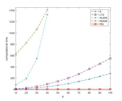
(a) regression

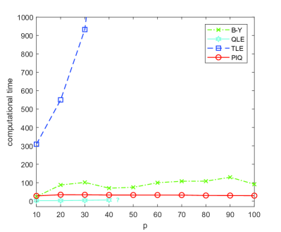
(b) classification

Figure 1: Computational time comparison between different robust methods as $p$ increases. Left: regression with $o^{*}=0.1n$ and $n=1000$ (RLARS and PENSE are too costly compared with the other methods and only parts of their cost curves are shown). Right: classification with $o^{*}=0.05n$ and $n=1000$ (when $p>40$, QLE delivered an error message and could not continue).

Table 1 shows a performance comparison for robust regression and robust classification in Example 1 and Example 2, respectively. To investigate algorithm scalability, we also give a computational time comparison in Figure 1 with respect to the dimension $p$. According to the table, with less than $5\%$ outliers, all methods show satisfactory results for regression or classification. But as the percentage of outliers goes up to $10\%$ (say) or more, the performance of many conventional methods degrades significantly. Also, some algorithms have poor numerical stability as $p$ is just over 40. In comparison, PIQ is much more accurate and robust, and its scalability is evident.

Table 2: Performance comparison in $p>n$ settings (Example 3, Example 4 with $n=200,p=1000$). The outlier percentage varies from 5% to 20%.

	Regression
	$o^{*}=10$							$o^{*}=20$
	Err	Mγ	JDγ	Mβ	FAβ	JDβ	T		Err	Mγ	JDγ	Mβ	FAβ	JDβ	T
QL	0.37	36	16	19	0.1	40	43		0.71	81	0	25	0.2	24	42
S-MTE	0.44	73	0	14	0.2	54	35		0.64	82	0	18	0.2	48	39
RLARS	0.53	82	4	25	0.2	40	42		1.06	89	0	42	0.3	0	42
S-LTS	0.28	4	80	1	0.1	98	134		0.27	5	74	1	0.2	96	134
PIQ	0.11	2	86	3	0.2	90	4		0.23	5	80	10	0.2	64	4
	$o^{*}=30$							$o^{*}=40$
	Err	Mγ	JDγ	Mβ	FAβ	JDβ	T		Err	Mγ	JDγ	Mβ	FAβ	JDβ	T
QL	0.89	81	0	33	0.2	8	45		1.10	76	0	41	0.2	4	50
S-MTE	0.82	79	0	28	0.2	26	42		0.97	75	0	34	0.2	14	54
RLARS	1.52	91	0	58	0.3	0	41		1.55	85	0	57	0.3	0	40
S-LTS	1.24	79	10	29	1.4	16	132		1.52	82	0	46	1.5	0	136
PIQ	0.34	3	78	16	0.3	46	4		0.62	5	76	27	0.3	22	4
	Classification
	$o^{*}=10$							$o^{*}=20$
	Err	Mγ	JDγ	Mβ	FAβ	JDβ	T		Err	Mγ	JDγ	Mβ	FAβ	JDβ	T
enetLTS	12.4	4	96	1.3	0.1	96	62		16.0	22	78	5.3	0.24	86	67
PIQ	11.0	0	100	0	0.1	100	16		11.6	0	100	0	0.1	100	16
	$o^{*}=30$							$o^{*}=40$
	Err	Mγ	JDγ	Mβ	FAβ	JDβ	T		Err	Mγ	JDγ	Mβ	FAβ	JDβ	T
enetLTS	36.2	94	6	43	1.0	16	86		19.8	100	0	66	0.9	0	96
PIQ	12.6	0	100	0.7	0.1	98	14		17.0	8	84	9	0.1	78	14

The advantages of PIQ are even more impressive in Table 2 which summarizes the high-dimensional results. In particular, its boost in accuracy and outlier-resistance is not accompanied by a sacrifice in computational time relative to other robust methods. PIQ offered substantial time savings: its computational cost was at most about one fourth of that of the other algorithms.

We also conducted experiments with different correlation strengths, covariance structures and sparsity levels, and similar conclusions can be drawn from the performance comparison; see Appendix A.12 for details.

6.2 Robust classification of spam email

The email spam dataset (available at ftp.ics.uci.edu) contains 57 predictors including relative frequencies of 54 most commonly occurring words and characters and 3 statistics of capital letters. The total number of emails is 4,601, of which 1,813 are spam ($y=1$) and 2,788 are non-spam ($y=0$). We would like to know whether accommodating mislabeled emails (if any) could lead to improved spam/non-spam classification.

We applied PIQ with the logistic deviance and the Huberized hinge loss (Chapelle,, 2007), denoted by PIQ-L and PIQ-H, respectively, with PIC for tuning. Table 3 compares PIQ with logistic regression, B-Y, TLE, and QLE (cf. Section 6.1) in terms of misclassification error and F1-score (Chinchor,, 1992), both averaged over 100 data splits ($70\%$ for training and $30\%$ for test). From the table, TLE and QLE failed due to the large sample size. PIQ outperforms the other methods and the choice of the loss does not affect its performance on this dataset.

Table 3: Email spam data: misclassification error rates and F1-scores.

	Miscls (%)	F1 (%)
Logistic	7.5	90.3
B-Y	7.0	89.4
TLE	–	–
QLE	–	–
PIQ-L	6.8	91.3
PIQ-H	6.8	91.3

We then studied the subset of outliers identified by PIQ. Take PIQ-L for instance: there are 73 nonzeros $\hat{\gamma}_{i}$’s, the smallest magnitude being 10.97. To verify if there is indeed a distinction between the outliers ($o=1$) and clean observations ($o=0$), we examined 6 indicative features, free, !, $, hp, 650 and cap_avg. The first three words and signs are often used in spam to attract people’s attention; hp and 650 are related to the data creator’s working company and area code; cap_avg measures the average length of uninterrupted sequences of capital letters. Given each feature, we made a $2\times 2$ table with its rows corresponding to spam and non-spam ($y=1$, $0$) and columns corresponding to outlying and clean ($o=1$, $0$). The cross-product ratio or odds ratio visualizes the strong association between $y$ and $o$, as shown in Figure 2. Indeed, even the odds ratios closer to 1 are either as small as $\exp(-2.8)=0.06$ or as large as $\exp(4.89)=133$, demonstrating a strong discrepancy between the outlier subset and the clean subset. We also built an ANOVA model on each feature to test the significance of $o$; all the obtained $p$-values are below 1e-10, a clear evidence of the outlyingness.

The data analysis suggests that even on some conventional datasets, mislabeling frequently occurs and guarding against outliers is beneficial. It is fair to say that modern statistical analysis involves more and more large-scale datasets, but with bigger data also come more junk and errors. This could be a severe issue for binary classification, since any inaccuracy in labeling simply means the response goes to the other extreme. Applying a classifier designed under no consideration of gross outliers could be risky in reality, and our resistant learning framework offers an effective fix in this regard.

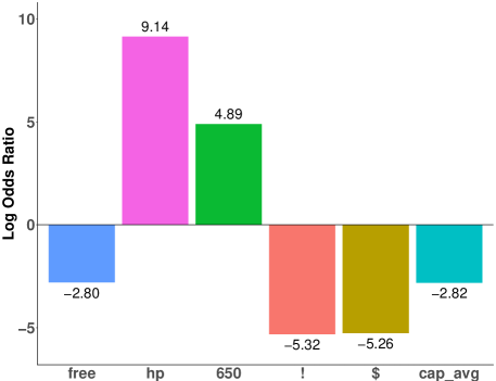
Figure 2: Log odds ratios of six $2\times 2$ tables with row variable $y$ and column variable $o$.

6.3 Robust neural network for Parkinson’s disease detection

Neural networks have attracted a great deal of attention in machine learning. In this experiment, we adapt the PIQ technique to a neural net model and test its performance for Parkinson’s disease (PD) detection. There has been a surge of interest in speech analysis of PD recently, as voice recordings from these patients tend to show typical patterns like aperiodic vibrations. We use the dataset from Little et al., (2007) which collects a range of biomedical voice measurements from normal people and patients with PD, where the 22 predictors for 195 recordings include various measures of vocal fundamental frequency and variation in amplitude, as well as some nonlinear metrics constructed from raw voice recordings. We randomly split the dataset into a training subset (60%) and a test subset (40%).

Previous studies suggest the presence of nonlinear effects and interactions of the features in this challenging classification task (Little et al., (2007), Sakar et al., (2013)). Hence we designed a feedforward neural network that consists of an input layer, two dense layers with 22 and 12 nodes respectively, and one output layer. The dense layers deploy the popular rectified linear units (ReLU) (Nair and Hinton,, 2010), and the output node uses a softmax activation. We trained the network for 200 epochs and attained a misclassification error rate of 9.1% on the test data—in contrast, an SVM with a nonlinear RBF kernel gave 17.9%. (Meanwhile, classical robust classification methods like B-Y, QLE, and TLE all behaved poorly, with the misclassification error rates $>25\%$.)

On the other hand, the noisy signals and potential outliers occurring suggest the need of robustification. But the overall network criterion barely resembles that of regression or logistic regression due to its substantial nonlinearity and hierarchy, and how to reweight the samples in this sophisticated model to limit the influence of outliers sounds tricky. Following the additive robustification scheme, we simply added sample-indicator features into the input layer (cf. Figure 3), accompanied by a group $\ell_{0}+\ell_{2}$ regularization ($q=0.05n$, $\nu=$ 1e-4) to correct for sample outlyingness in constructing predictive factors. Our optimization-based PIQ algorithm can be seamlessly incorporated into the process of back-propagation. Though a simple modification, the robustified neural network gave an impressive misclassification error rate 6.4%, an improvement of about 30% over that of the vanilla neural network.

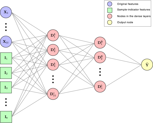
Figure 3: Structure of the robustified neural network on Parkinson’s disease data, where sample-indicator features (denoted by green square nodes) are added to the input layer.

7 Summary

The work studied how to gain outlier resistance for a given loss that is not necessarily quadratic and may go beyond the likelihood setup. Motivated by the method of trimming, we proposed an $\ell_{0}$+$\ell_{2}$ regularized learning framework. We showed that pursuing its (global) minimizers can cope with extreme outliers regardless of leverage and outlyingness, but on large-scale data, there is always a balance between statistical accuracy and computational efficiency. Hence a more meaningful and deeper question is how to design a scalable algorithm to alleviate the starting point requirement and the regularity conditions to obtain the desired order of statistical accuracy.

In this work, the interplay between high dimensional statistics and nonconvex optimization led to fruitful results for resistant learning on the learning rate, cardinality control, the choice of regularization parameters, and so on. In particular, a novel progressive backward optimization scheme is brought forward which, unlike subset sampling, is cost effective, and can significantly improve the statistical performance of iterative quantile-thresholding. We hope that the work could raise concern about outliers among (big) data analysts, as well as providing a sensible and universal means to boosting resistance in regression, classification and more sophisticated learning tasks.

Appendix A Proofs

A.1 Proof of Theorem 1

First, we introduce a lemma to be used for proving the three statements.

Lemma 1.

Let $l_{0}(\eta;y)$ be a loss function defined on $\eta\in\mathbb{R}$ with $y\in\mathcal{Y}\subset\mathbb{R}$ as a parameter and $\inf_{\eta}l_{0}(\eta;y)=L>-\infty\mbox{ for all }y\in\mathcal{Y}$. Define ${\boldsymbol{\eta}}={\boldsymbol{X}}{\boldsymbol{\beta}}$ and $l({\boldsymbol{\eta}};{\boldsymbol{y}})=\sum_{i=1}^{n}l_{0}(\eta_{i};y_{i})$. Given any ${\boldsymbol{\beta}}$, let $l_{0}^{(1)}({\boldsymbol{\beta}})\leq\ldots\leq l_{0}^{(n)}({\boldsymbol{\beta}})$ be the order statistics of $l_{0}({\boldsymbol{x}}_{i}^{T}{\boldsymbol{\beta}};y_{i})$ ($1\leq i\leq n$). Then

$$\inf_{\|{\boldsymbol{\gamma}}\|_{0}\leq q}l({\boldsymbol{X}}{\boldsymbol{\beta}}+{\boldsymbol{\gamma}};{\boldsymbol{y}})=\sum_{i=1}^{n-q}l_{0}^{(i)}({\boldsymbol{\beta}}).$$ (A.1)

Moreover, given any $\tau\geq 0$,

$$\inf_{{\boldsymbol{\gamma}}}\,l({\boldsymbol{X}}{\boldsymbol{\beta}}+{\boldsymbol{\gamma}};{\boldsymbol{y}})+\tau\|{\boldsymbol{\gamma}}\|_{0}=\sum_{i=1}^{n}(\tau+L)\wedge l_{0}({\boldsymbol{x}}_{i}^{T}{\boldsymbol{\beta}};y_{i}).$$ (A.2)

For a), let $(\hat{\boldsymbol{\beta}},\hat{\boldsymbol{\gamma}})$ be a globally optimal solution to

$$\min_{({\boldsymbol{\beta}},{\boldsymbol{\gamma}})}l({\boldsymbol{\eta}};{\boldsymbol{y}})\mbox{ s.t. }{\boldsymbol{\eta}}={\boldsymbol{X}}{\boldsymbol{\beta}}+{\boldsymbol{\gamma}},\mbox{ }\|{\boldsymbol{\gamma}}\|_{0}\leq q.$$ (A.3)

Then for any ${\boldsymbol{\beta}}$, $l({\boldsymbol{X}}\hat{\boldsymbol{\beta}}+\hat{\boldsymbol{\gamma}};{\boldsymbol{y}})\leq l({\boldsymbol{X}}{\boldsymbol{\beta}}+\hat{\boldsymbol{\gamma}}_{\boldsymbol{\beta}};{\boldsymbol{y}}),$ where $\hat{\boldsymbol{\gamma}}_{\boldsymbol{\beta}}$ is an optimal solution of ${\boldsymbol{\gamma}}$ given ${\boldsymbol{\beta}}$. From Lemma 1, $l({\boldsymbol{X}}\hat{\boldsymbol{\beta}}+\hat{\boldsymbol{\gamma}};{\boldsymbol{y}})=\sum_{i=1}^{n-q}l_{0}^{(i)}(\hat{\boldsymbol{\beta}}),\mbox{ }l({\boldsymbol{X}}{\boldsymbol{\beta}}+\hat{\boldsymbol{\gamma}}_{\boldsymbol{\beta}};{\boldsymbol{y}})=\sum_{i=1}^{n-q}l_{0}^{(i)}({\boldsymbol{\beta}}),$ and so $\sum_{i=1}^{n-q}l_{0}^{(i)}(\hat{\boldsymbol{\beta}})\leq\sum_{i=1}^{n-q}l_{0}^{(i)}({\boldsymbol{\beta}}).$

Now suppose that $\hat{\boldsymbol{\beta}}$ is a globally optimal solution that minimizes the trimmed criterion on the RHS of (A.1). Then for any $({\boldsymbol{\beta}},{\boldsymbol{\gamma}})$,

$$l({\boldsymbol{X}}{\boldsymbol{\beta}}+{\boldsymbol{\gamma}};{\boldsymbol{y}}) \geq l({\boldsymbol{X}}{\boldsymbol{\beta}}+\hat{\boldsymbol{\gamma}}_{\boldsymbol{\beta}};{\boldsymbol{y}})=\sum_{i=1}^{n-q}l_{0}^{(i)}({\boldsymbol{\beta}})\geq\sum_{i=1}^{n-q}l_{0}^{(i)}(\hat{\boldsymbol{\beta}})=l({\boldsymbol{X}}\hat{\boldsymbol{\beta}}+\hat{\boldsymbol{\gamma}}_{\hat{\boldsymbol{\beta}}};{\boldsymbol{y}}),$$

which means $(\hat{\boldsymbol{\beta}};\hat{\boldsymbol{\gamma}}_{\hat{\boldsymbol{\beta}}})$ is a global minimizer of (A.3). The second conclusion for the penalized form and winsorized form can be proved similarly (assuming $L=0$).

To prove the last statement, we set $\mathcal{C}({\boldsymbol{\beta}})=\{i:l_{0}({\boldsymbol{x}}_{i}^{T}{\boldsymbol{\beta}};y_{i})>\tau,1\leq i\leq n\}$ and $c({\boldsymbol{\beta}})=|\mathcal{C}({\boldsymbol{\beta}})|$. So $\sum_{i=1}^{n}\tau\wedge l_{0}({\boldsymbol{x}}_{i}^{T}{\boldsymbol{\beta}};y_{i})=c({\boldsymbol{\beta}})\tau+\sum_{i=1}^{n-c({\boldsymbol{\beta}})}l_{0}^{(i)}({\boldsymbol{\beta}})$.

We claim that for any $\hat{\boldsymbol{\beta}}\in\arg\min\sum\tau\wedge l_{0}({\boldsymbol{x}}_{i}^{T}{\boldsymbol{\beta}};y_{i})$ with $q=c(\hat{\boldsymbol{\beta}})$, it is also an optimal solution to $\min\sum_{i=1}^{n-q}l_{0}^{(i)}({\boldsymbol{\beta}})$. Prove by contradiction: if $\sum_{i=1}^{n-q}l_{0}^{(i)}(\hat{\boldsymbol{\beta}})>\sum_{i=1}^{n-q}l_{0}^{(i)}({\boldsymbol{\beta}})$ for some ${\boldsymbol{\beta}}$, then since $\tau\wedge l_{0}({\boldsymbol{x}}_{i}^{T}\hat{\boldsymbol{\beta}};y_{i})=\tau\geq\tau\wedge l_{0}({\boldsymbol{x}}_{j}^{T}{\boldsymbol{\beta}};y_{j})$ for all $i\in\mathcal{C}(\hat{\boldsymbol{\beta}}),j:1\leq j\leq n$, we would get $\sum_{i=1}^{n}\tau\wedge l_{0}({\boldsymbol{x}}_{i}^{T}\hat{\boldsymbol{\beta}};y_{i})>\sum_{i=1}^{n}\tau\wedge l_{0}({\boldsymbol{x}}_{i}^{T}{\boldsymbol{\beta}};y_{i})$.

Finally, we show that given any $(\hat{\boldsymbol{\beta}},\hat{\boldsymbol{\gamma}})\in\arg\min l({\boldsymbol{X}}{\boldsymbol{\beta}}+{\boldsymbol{\gamma}};{\boldsymbol{y}})+\tau\|{\boldsymbol{\gamma}}\|_{0}$ with $q=\|\hat{\boldsymbol{\gamma}}\|_{0}$ (where $\hat{\gamma}_{i}$ are allowed to take $\pm\infty$), it is also an optimal solution to $\min_{{\boldsymbol{\beta}},{\boldsymbol{\gamma}}}l({\boldsymbol{X}}{\boldsymbol{\beta}}+{\boldsymbol{\gamma}};{\boldsymbol{y}})\mbox{ s.t. }\|{\boldsymbol{\gamma}}\|_{0}\leq q$. Suppose that there exists $({\boldsymbol{\beta}},{\boldsymbol{\gamma}})$ with $\|{\boldsymbol{\gamma}}\|_{0}\leq q$ so that $l({\boldsymbol{X}}\hat{\boldsymbol{\beta}}+\hat{\boldsymbol{\gamma}};{\boldsymbol{y}})>l({\boldsymbol{X}}{\boldsymbol{\beta}}+{\boldsymbol{\gamma}};{\boldsymbol{y}})$. Then, by considering $({\boldsymbol{\beta}},{\boldsymbol{\gamma}}^{\prime})$ with ${\boldsymbol{\gamma}}^{\prime}=\hat{\boldsymbol{\gamma}}_{\boldsymbol{\beta}}$ and $\|{\boldsymbol{\gamma}}^{\prime}\|_{0}\leq q$ as defined previously, $\inf_{\|{\boldsymbol{\gamma}}\|_{0}\leq q}l({\boldsymbol{X}}\hat{\boldsymbol{\beta}}+{\boldsymbol{\gamma}};{\boldsymbol{y}})=l({\boldsymbol{X}}\hat{\boldsymbol{\beta}}+\hat{\boldsymbol{\gamma}};{\boldsymbol{y}})>\inf_{\|{\boldsymbol{\gamma}}\|_{0}\leq q}l({\boldsymbol{X}}{\boldsymbol{\beta}}+{\boldsymbol{\gamma}};{\boldsymbol{y}})$, and thus $\sum_{i=1}^{n-q}l_{0}^{(i)}(\hat{\boldsymbol{\beta}})>\sum_{i=1}^{n-q}l_{0}^{(i)}({\boldsymbol{\beta}})$ from Lemma 1. Using the fact that $\hat{\gamma}_{i}\neq 0$ implies $\tau+l_{0}({\boldsymbol{x}}_{i}^{T}\hat{\boldsymbol{\beta}}+\hat{\gamma}_{i};y_{i})=\tau$, and the construction of ${\boldsymbol{\gamma}}^{\prime}$, $l({\boldsymbol{X}}\hat{\boldsymbol{\beta}}+\hat{\boldsymbol{\gamma}};{\boldsymbol{y}})+\tau\|\hat{\boldsymbol{\gamma}}\|_{0}=q\tau+\sum_{i=1}^{n-q}l_{0}^{(i)}(\hat{\boldsymbol{\beta}})$ and $l({\boldsymbol{X}}{\boldsymbol{\beta}}+{\boldsymbol{\gamma}}^{\prime};{\boldsymbol{y}})+\tau\|{\boldsymbol{\gamma}}^{\prime}\|_{0}=q\tau+\sum_{i=1}^{n-q}l_{0}^{(i)}({\boldsymbol{\beta}})$. Summarizing the above gives $l({\boldsymbol{X}}\hat{\boldsymbol{\beta}}+\hat{\boldsymbol{\gamma}};{\boldsymbol{y}})>l({\boldsymbol{X}}{\boldsymbol{\beta}}+{\boldsymbol{\gamma}}^{\prime};{\boldsymbol{y}})$, contradicting the optimality of $(\hat{\boldsymbol{\beta}},\hat{\boldsymbol{\gamma}})$. The proof is complete.

Proof of Lemma 1

Recall that the loss is assumed bounded from below. Without loss of generality, let $\inf_{\eta}l_{0}(\eta;y)=0\mbox{ for all }y\in\mathcal{Y}$ (otherwise, we can redefine the loss function by $l_{0}(\eta;y)-\inf_{\eta}l_{0}(\eta;y)$).

Given $\boldsymbol{\beta}$, denote by $\hat{\boldsymbol{\gamma}}_{\boldsymbol{\beta}}$ a minimizer of $l(\boldsymbol{X}\boldsymbol{\beta}+\boldsymbol{\gamma};\boldsymbol{y})$ subject to $\|\boldsymbol{\gamma}\|_{0}\leq q$, whose components can take $\pm\infty$. Then if $\hat{\gamma}_{i}=0$, $l_{0}({\boldsymbol{x}}_{i}^{T}{\boldsymbol{\beta}}+\hat{\gamma}_{i};y_{i})=l_{0}({\boldsymbol{x}}_{i}^{T}{\boldsymbol{\beta}};y_{i})\geq 0$. If $\hat{\gamma}_{i}\neq 0$, by varying its value, which will not violate the constraint, one can argue that $l_{0}({\boldsymbol{x}}_{i}^{T}{\boldsymbol{\beta}}+\hat{\gamma}_{i};y_{i})=\inf_{\eta}l_{0}(\eta;y_{i})=0$. Therefore, $l({\boldsymbol{X}}{\boldsymbol{\beta}}+\hat{\boldsymbol{\gamma}}_{{\boldsymbol{\beta}}};{\boldsymbol{y}})=\sum_{i=1}^{n-q}l_{0}^{(i)}({\boldsymbol{\beta}})$. The proof of (A.2) follows similar lines.

A.2 Proof of Theorem 2

First, we have the following result to argue the (alternative) optimality of ${\boldsymbol{\gamma}}^{(t+1)}$ given ${\boldsymbol{\beta}}^{(t)}$, cf. Lemma C.1 in She et al., (2013).

Lemma 2.

Given any $\boldsymbol{s}\in\mathbb{R}^{n}$, $0\leq q\leq n$, $\nu\geq 0$, $\hat{\boldsymbol{\xi}}=\Theta^{\#}(\boldsymbol{s};q,\nu)$ is a global optimal solution to $\min_{{\boldsymbol{\xi}}\in\mathbb{R}^{n}}\|\boldsymbol{s}-{\boldsymbol{\xi}}\|_{2}^{2}/2+\nu\|{\boldsymbol{\xi}}\|_{2}^{2}/2\mbox{ s.t. }\|{\boldsymbol{\xi}}\|_{0}\leq q.$

The below definition of a sub-Gaussian random vector is standard in the literature, see, e.g., Vershynin, (2012).

Definition 1 (Sub-Gaussian random variable/vector).

We call $\xi$ a sub-Gaussian(0, $\sigma^{2}$) random variable if and only if $\xi$ has mean 0 and there exist constants $C,c>0$ such that $\mathbb{P}\{|\xi|\geq t\}\leq Ce^{-ct^{2}},\forall t>0$ with the scale (or $\psi_{2}$-norm) of $\xi$ defined by $\sigma(\xi)=\inf\{\sigma>0:\mathbb{E}\exp(\xi^{2}/\sigma^{2})\leq 2\}$. More generally, $\boldsymbol{\xi}\in\mathbb{R}^{p}$ is called a sub-Gaussian random vector with scale bounded by $\sigma$ if all one-dimensional marginals $\langle\boldsymbol{\xi},\boldsymbol{\alpha}\rangle$ are sub-Gaussian satisfying $\|\langle\boldsymbol{\xi},\boldsymbol{\alpha}\rangle\|_{\psi_{2}}\leq\sigma\|\boldsymbol{\alpha}\|_{2}$, $\forall\boldsymbol{\alpha}\in\mathbb{R}^{p}$.

a) Using the update in (6), we can represent the optimal ${\boldsymbol{\beta}}$ as a function of ${\boldsymbol{\gamma}}$, from which problem (5) is equivalent to

$$\min_{\boldsymbol{\gamma}}f(\boldsymbol{\gamma}):=\frac{1}{2}\|(\boldsymbol{I}-\boldsymbol{H})(\boldsymbol{\gamma}-\boldsymbol{y})\|_{2}^{2}+\frac{\nu}{2}\|\boldsymbol{\gamma}\|_{2}^{2}\text{ s.t. }\|\boldsymbol{\gamma}\|_{0}\leq q.$$ (A.4)

Let $l(\boldsymbol{\gamma})=\|(\boldsymbol{I}-\boldsymbol{H})(\boldsymbol{\gamma}-\boldsymbol{y})\|_{2}^{2}/2$. From Lemma 2, a nice fact of (7) is that

$$\boldsymbol{\gamma}^{(t+1)}=\arg\min_{\|\boldsymbol{\gamma}\|_{0}\leq q}g(\boldsymbol{\gamma};\boldsymbol{\gamma}^{(t)}),$$

where

$$g(\boldsymbol{\gamma};\boldsymbol{\gamma}^{-}) =\|(\boldsymbol{I}-\boldsymbol{H})(\boldsymbol{\gamma}^{-}-\boldsymbol{y})\|_{2}^{2}/2+\langle(\boldsymbol{I}-\boldsymbol{H})(\boldsymbol{\gamma}^{-}-\boldsymbol{y}),\boldsymbol{\gamma}-\boldsymbol{\gamma}^{-}\rangle$$

$$\quad+\|\boldsymbol{\gamma}-\boldsymbol{\gamma}^{-}\|_{2}^{2}/2+\nu\|\boldsymbol{\gamma}\|_{2}^{2}/2$$

$$=f(\boldsymbol{\gamma})+(\mathbf{D}_{2}-\boldsymbol{\Delta}_{l})(\boldsymbol{\gamma},\boldsymbol{\gamma}^{-})$$

with $\boldsymbol{\Delta}_{l}$ and $\mathbf{D}_{2}$ introduced in Section 4. By definition, $g(\boldsymbol{\gamma}^{(t)};\boldsymbol{\gamma}^{(t)})\geq g(\boldsymbol{\gamma}^{(t+1)};\boldsymbol{\gamma}^{(t)})$, and so we have

$$f(\boldsymbol{\gamma}^{(t)})-f(\boldsymbol{\gamma}^{(t+1)})\geq(\mathbf{D}_{2}-\boldsymbol{\Delta}_{l})(\boldsymbol{\gamma}^{(t+1)},\boldsymbol{\gamma}^{(t)}).$$ (A.5)

Summing up (A.5) over $t=1,\ldots,T$ gives the conclusion.

b) We begin with a useful lemma. Throughout the proof, given any ${\boldsymbol{\beta}}$, we use $\mathcal{J}({\boldsymbol{\beta}})$ to denote its support, i.e., $\mathcal{J}({\boldsymbol{\beta}})=\{j:\beta_{j}\neq 0\}$, and $J({\boldsymbol{\beta}})=|\mathcal{J}({\boldsymbol{\beta}})|$. Recall that $s^{*}=J({\boldsymbol{\beta}}^{*})$ and $o^{*}=J({\boldsymbol{\gamma}}^{*})$.

Lemma 3.

Given $q\leq p$ and $\nu\geq 0$, a globally optimal solution to the optimization problem $\min_{\boldsymbol{\beta}\in\mathbb{R}^{p}}l(\boldsymbol{\beta})=\|\boldsymbol{y}-\boldsymbol{\beta}\|_{2}^{2}/2+\nu\|\boldsymbol{\beta}\|_{2}^{2}/2$ s.t. $\|\boldsymbol{\beta}\|_{0}\leq q$ is given by $\hat{\boldsymbol{\beta}}=\Theta^{\#}(\boldsymbol{y};q,\nu)$. Let $\mathcal{J}=\mathcal{J}(\boldsymbol{\beta})$, $\hat{\mathcal{J}}=\mathcal{J}(\hat{\boldsymbol{\beta}})$ and assume $J(\hat{\boldsymbol{\beta}})=q$. Then, for any $\boldsymbol{\beta}$ with $J(\boldsymbol{\beta})\leq s=q/\vartheta$ and $\vartheta\geq 1$,

$$l(\boldsymbol{\beta})-l(\hat{\boldsymbol{\beta}})\geq\{1-\mathcal{L}(\mathcal{J},\hat{\mathcal{J}})\}(1+\nu)\|\hat{\boldsymbol{\beta}}-\boldsymbol{\beta}\|_{2}^{2}/2,$$

where $\mathcal{L}(\mathcal{J},\hat{\mathcal{J}})=(|\mathcal{J}\backslash\hat{\mathcal{J}}|/|\hat{\mathcal{J}}\backslash\mathcal{J}|)^{1/2}\leq(s/q)^{1/2}=\vartheta^{-1/2}$.

It can be proved by Lemma 9 in She and Chen, (2017). By Lemma 3, for any ${\boldsymbol{\gamma}}$ satisfying $\|{\boldsymbol{\gamma}}\|_{0}\leq q$,

$$g(\boldsymbol{\gamma};\boldsymbol{\gamma}^{(t)})-g(\boldsymbol{\gamma}^{(t+1)};\boldsymbol{\gamma}^{(t)})\geq\{1-\mathcal{L}(\mathcal{J}(\boldsymbol{\gamma}),\mathcal{J}(\boldsymbol{\gamma}^{(t+1)}))\}(1+\nu)\mathbf{D}_{2}(\boldsymbol{\gamma}^{(t+1)},\boldsymbol{\gamma}),$$

and so

$$\begin{split}&f(\boldsymbol{\gamma})+(\mathbf{D}_{2}-\boldsymbol{\Delta}_{l})(\boldsymbol{\gamma},\boldsymbol{\gamma}^{(t)})-f(\boldsymbol{\gamma}^{(t+1)})-(\mathbf{D}_{2}-\boldsymbol{\Delta}_{l})(\boldsymbol{\gamma}^{(t+1)},\boldsymbol{\gamma}^{(t)})\\ \geq\,&\{1-\mathcal{L}(\mathcal{J}(\boldsymbol{\gamma}),\mathcal{J}(\boldsymbol{\gamma}^{(t+1)}))\}(1+\nu)\mathbf{D}_{2}(\boldsymbol{\gamma}^{(t+1)},\boldsymbol{\gamma}),\end{split}$$

or

$$\begin{split}&f(\boldsymbol{\gamma})+((1+\nu)\mathbf{D}_{2}-\boldsymbol{\Delta}_{f})(\boldsymbol{\gamma},\boldsymbol{\gamma}^{(t)})-f(\boldsymbol{\gamma}^{(t+1)})-(\mathbf{D}_{2}-\boldsymbol{\Delta}_{l})(\boldsymbol{\gamma}^{(t+1)},\boldsymbol{\gamma}^{(t)})\\ \geq\,&\{1-\mathcal{L}(\mathcal{J}(\boldsymbol{\gamma}),\mathcal{J}(\boldsymbol{\gamma}^{(t+1)}))\}(1+\nu)\mathbf{D}_{2}(\boldsymbol{\gamma}^{(t+1)},\boldsymbol{\gamma}).\end{split}$$

Substituting $\boldsymbol{\gamma}^{*}$ for ${\boldsymbol{\gamma}}$ gives

$$\begin{split}&\{1-\mathcal{L}(\mathcal{J}(\boldsymbol{\gamma}^{*}),\mathcal{J}(\boldsymbol{\gamma}^{(t+1)}))\}(1+\nu)\mathbf{D}_{2}(\boldsymbol{\gamma}^{(t+1)},\boldsymbol{\gamma}^{*})+(\mathbf{D}_{2}-\boldsymbol{\Delta}_{l})(\boldsymbol{\gamma}^{(t+1)},\boldsymbol{\gamma}^{(t)})\\ \leq\,&-\boldsymbol{\Delta}_{f}(\boldsymbol{\gamma}^{(t+1)},\boldsymbol{\gamma}^{*})-\langle\nabla f(\boldsymbol{\gamma}^{*}),\boldsymbol{\gamma}^{(t+1)}-\boldsymbol{\gamma}^{*}\rangle+((1+\nu)\mathbf{D}_{2}-\boldsymbol{\Delta}_{f})(\boldsymbol{\gamma}^{*},\boldsymbol{\gamma}^{(t)}).\end{split}$$ (A.6)

Since $\|{\boldsymbol{I}}-{\boldsymbol{H}}\|_{2}=1$, $(\mathbf{D}_{2}-\boldsymbol{\Delta}_{l})(\boldsymbol{\gamma}^{(t+1)},\boldsymbol{\gamma}^{(t)})\geq 0$. Together with

$$\mathcal{L}(\mathcal{J}(\boldsymbol{\gamma}^{*}),\allowbreak\mathcal{J}(\boldsymbol{\gamma}^{(t+1)}))\leq 1/\sqrt{\vartheta},$$

we obtain

$$\begin{split}&((1-1/\sqrt{\vartheta})(1+\nu)\mathbf{D}_{2}+\boldsymbol{\Delta}_{l}+\nu\mathbf{D}_{2})(\boldsymbol{\gamma}^{(t+1)},\boldsymbol{\gamma}^{*})\\ \leq\,&(\mathbf{D}_{2}-\boldsymbol{\Delta}_{l})(\boldsymbol{\gamma}^{*},\boldsymbol{\gamma}^{(t)})+\langle(\boldsymbol{I}-\boldsymbol{H})^{2}(\boldsymbol{\gamma}^{*}-\boldsymbol{y})+\nu\boldsymbol{\gamma}^{*},-\boldsymbol{\gamma}^{(t+1)}+\boldsymbol{\gamma}^{*}\rangle\\ =\,&(\mathbf{D}_{2}-\boldsymbol{\Delta}_{l})(\boldsymbol{\gamma}^{*},\boldsymbol{\gamma}^{(t)})+\langle-\boldsymbol{U}_{\perp}\boldsymbol{U}_{\perp}^{T}\boldsymbol{\epsilon}+\nu\boldsymbol{\gamma}^{*},\boldsymbol{\gamma}^{*}-\boldsymbol{\gamma}^{(t+1)}\rangle\\ =\,&(\mathbf{D}_{2}-\boldsymbol{\Delta}_{l})(\boldsymbol{\gamma}^{*},\boldsymbol{\gamma}^{(t)})+\langle\boldsymbol{\epsilon}^{\prime},\boldsymbol{U}_{\perp}^{T}(\boldsymbol{\gamma}^{(t+1)}-\boldsymbol{\gamma}^{*})\rangle+\nu\langle\boldsymbol{\gamma}^{*},\boldsymbol{\gamma}^{*}-\boldsymbol{\gamma}^{(t+1)}\rangle,\\ \end{split}$$ (A.7)

where $\boldsymbol{X}=[\boldsymbol{U},\boldsymbol{U}_{\perp}]\boldsymbol{D}\boldsymbol{V}^{T}$ is the singular value decomposition of $\boldsymbol{X}$ with $\boldsymbol{U}_{\perp}\in\mathbb{R}^{n\times(n-p)}$ and $\boldsymbol{\epsilon}^{\prime}=\boldsymbol{U}_{\perp}^{T}\boldsymbol{\epsilon}$ which is still a sub-Gaussian random vector with mean 0 and scaled bounded by $\sigma$. From ${\boldsymbol{I}}-{\boldsymbol{H}}={\boldsymbol{U}}_{\perp}{\boldsymbol{U}}_{\perp}^{T}$, $\Delta_{l}(\boldsymbol{\gamma},\boldsymbol{\gamma}^{\prime})=\|{\boldsymbol{U}}_{\perp}^{T}({\boldsymbol{\gamma}}-{\boldsymbol{\gamma}}^{\prime})\|_{2}^{2}/2$.

The stochastic term $\langle\boldsymbol{\epsilon}^{\prime},\boldsymbol{U}_{\perp}^{T}(\boldsymbol{\gamma}^{(t+1)}-\boldsymbol{\gamma}^{*})\rangle$ can be bounded using the following lemma.

Lemma 4.

Let $\boldsymbol{\epsilon}$ be a sub-Gaussian random vector with mean zero and scale bounded by $\sigma$. Given $\boldsymbol{X}\in\mathbb{R}^{n\times p}$ and $0\leq J\leq p$, there exist universal constants $A,C,c>0$ such that for any $a>0$, the following event

$$\sup_{{\boldsymbol{\beta}}\in\mathbb{R}^{p}:\|{\boldsymbol{\beta}}\|_{0}\leq J}\langle\boldsymbol{\epsilon},\boldsymbol{X}{\boldsymbol{\beta}}\rangle-\frac{1}{2a}\|\boldsymbol{X}{\boldsymbol{\beta}}\|_{2}^{2}-aA^{2}\sigma^{2}J\log(ep/J)>a\sigma^{2}t$$ (A.8)

occurs with probability at most $C\exp(-ct)p^{-cA^{2}}$ for any $t\geq 0$.

The result is a variant of Lemma 4 of She, (2016) and can be obtained from its proof. According to Lemma 4, there exist constants $A,C,c>0$ such that for any $a>0$,

$$\langle\boldsymbol{\epsilon}^{\prime},\boldsymbol{U}_{\perp}^{T}(\boldsymbol{\gamma}^{(t+1)}-\boldsymbol{\gamma}^{*})\rangle\leq\frac{1}{a}\boldsymbol{\Delta}_{l}(\boldsymbol{\gamma}^{(t+1)},\boldsymbol{\gamma}^{*})+aA^{2}\sigma^{2}(1+\vartheta)o^{*}\log\frac{en}{o^{*}}$$ (A.9)

occurs with probability at least $1-C(n-p)^{-c}$. Since $\langle\boldsymbol{\gamma}^{*},-\boldsymbol{\gamma}^{(t+1)}+\boldsymbol{\gamma}^{*}\rangle\leq(b/2)\|\boldsymbol{\gamma}^{*}\|_{2}^{2}+(1/2b)\|\boldsymbol{\gamma}^{(t+1)}-\boldsymbol{\gamma}^{*}\|_{2}^{2}$ for any $b>0$, combining (A.7) and (A.9) gives

$$\begin{split}&\{((1-\frac{1}{\sqrt{\vartheta}})+(2-\frac{1}{\sqrt{\vartheta}}-\frac{1}{b})\nu)\mathbf{D}_{2}+(1-\frac{1}{a})\boldsymbol{\Delta}_{l}\}(\boldsymbol{\gamma}^{(t+1)},\boldsymbol{\gamma}^{*})\\ \leq\,&(\mathbf{D}_{2}-\boldsymbol{\Delta}_{l})(\boldsymbol{\gamma}^{(t)},\boldsymbol{\gamma}^{*})+aA^{2}\sigma^{2}(1+\vartheta)o^{*}\log\frac{en}{o^{*}}+\frac{b\nu}{2}\|\boldsymbol{\gamma}^{*}\|_{2}^{2}.\end{split}$$ (A.10)

Let

$$\kappa=\frac{1}{1-\varepsilon}\big{\{}(2-\frac{1}{a})\varepsilon-\frac{1}{\sqrt{\vartheta}}+(2-\frac{1}{\sqrt{\vartheta}}-\frac{1}{b})\nu\big{\}}.$$ (A.11)

By the regularity condition,

$$\begin{split}&(1+\kappa)(\mathbf{D}_{2}-\boldsymbol{\Delta}_{l})(\boldsymbol{\gamma}^{(t+1)},\boldsymbol{\gamma}^{*})\\ \leq\,&\{((1-\frac{1}{\sqrt{\vartheta}})+(2-\frac{1}{\sqrt{\vartheta}}-\frac{1}{b})\nu)\mathbf{D}_{2}+(1-\frac{1}{a})\boldsymbol{\Delta}_{l}\}(\boldsymbol{\gamma}^{(t+1)},\boldsymbol{\gamma}^{*})\\ \leq\,&(\mathbf{D}_{2}-\boldsymbol{\Delta}_{l})(\boldsymbol{\gamma}^{(t)},\boldsymbol{\gamma}^{*})+aA^{2}\sigma^{2}(1+\vartheta)o^{*}\log\frac{en}{o^{*}}+\frac{b\nu}{2}\|\boldsymbol{\gamma}^{*}\|_{2}^{2}.\end{split}$$

Finally, by a recursive argument, we have

$$\begin{split}&(\mathbf{D}_{2}-\boldsymbol{\Delta}_{l})(\boldsymbol{\gamma}^{(t)},\boldsymbol{\gamma}^{*})\\ \leq\,&\Big{(}\frac{1}{\kappa+1}\Big{)}^{t-1}(\mathbf{D}_{2}-\boldsymbol{\Delta}_{l})(\boldsymbol{\gamma}^{(1)},\boldsymbol{\gamma}^{*})+\frac{a}{\kappa}A^{2}\sigma^{2}(1+\vartheta)o^{*}\log\frac{en}{o^{*}}+\frac{b\nu}{2\kappa}\|\boldsymbol{\gamma}^{*}\|_{2}^{2}.\end{split}$$

Choosing $a=1$, $b=1$, which ensures $1+\kappa\geq 0$, we obtain the conclusion on the sequence of ${\boldsymbol{\gamma}}$-iterates.

In fact, according to (A.11), we may choose any $a\geq 1$ and $b>0$, and so the linear convergence rate holds if $\varepsilon>1/(2\sqrt{\vartheta})-(2-{1}/({\sqrt{\vartheta}})\nu$.

To show the conclusion on the sequence of ${\boldsymbol{\beta}}$-iterates, notice that for any $t\geq 1$,

$${\boldsymbol{X}}{\boldsymbol{\beta}}^{(t)}-{\boldsymbol{X}}{\boldsymbol{\beta}}^{*}+{\boldsymbol{H}}{\boldsymbol{\gamma}}^{(t)}-{\boldsymbol{H}}{\boldsymbol{\gamma}}^{*}={\boldsymbol{H}}{\boldsymbol{\epsilon}}.$$

and

$$\,\mathbb{P}[\|{\boldsymbol{H}}{\boldsymbol{\epsilon}}\|_{2}^{2}\geq cr({\boldsymbol{X}})\sigma^{2}+t\sigma^{2}]\leq C\exp(-c[\{t^{2}/r({\boldsymbol{X}})\}\wedge t]),$$

where $r({\boldsymbol{X}})$ denotes the rank of ${\boldsymbol{X}}$. The last inequality can be shown from the Hanson-Wright inequality (Rudelson and Vershynin,, 2013) under the independent sub-Gaussian assumption since $\|{\boldsymbol{H}}\|_{2}=1$ and $\|{\boldsymbol{H}}\|_{F}^{2}=r({\boldsymbol{X}})$. Then applying the Cauchy-Schwartz inequality gives the result (details omitted).

A.3 Proof of Theorem 3

First, a thresholding function (She and Owen,, 2011) is defined as a real-valued function $\Theta(t;\lambda)$ for $-\infty<t<\infty$ and $0\leq\lambda<\infty$ such that (i) $\Theta(-t;\lambda)=-\Theta(t;\lambda)$; (ii) $\Theta(t;\lambda)\leq\Theta(t^{\prime};\lambda)$ for $t\leq t^{\prime}$; (iii) $\mathop{\lim}_{t\rightarrow\infty}\Theta(t;\lambda)=\infty$; (iv) $0\leq\Theta(t;\lambda)\leq t$ for $0\leq t<\infty$. $\Theta$ is defined component-wise if either $t$ or $\lambda$ is replaced by a vector. Throughout the paper, assume that $\lambda$ is the threshold parameter.

Let $f(\bar{\boldsymbol{\beta}})=\tilde{l}(\bar{\boldsymbol{\beta}})+P(\varrho\boldsymbol{\beta};\lambda)+\nu\|\boldsymbol{\gamma}\|_{2}^{2}/2+\iota({\boldsymbol{\gamma}};q)$, where $\tilde{l}(\bar{\boldsymbol{\beta}})=l(\bar{\boldsymbol{X}}\bar{\boldsymbol{\beta}};\boldsymbol{y})$ and $\iota({\boldsymbol{\gamma}};q)=0$ if $\|{\boldsymbol{\gamma}}\|_{0}\leq q$ and $+\infty$ otherwise. Let $g(\bar{\boldsymbol{\beta}};\bar{\boldsymbol{\beta}}^{-})=l(\bar{\boldsymbol{X}}\bar{\boldsymbol{\beta}}^{-};{\boldsymbol{y}})+\langle\bar{\boldsymbol{X}}^{T}\nabla l(\bar{\boldsymbol{X}}\bar{\boldsymbol{\beta}}^{-};{\boldsymbol{y}}),\bar{\boldsymbol{\beta}}-\bar{\boldsymbol{\beta}}^{-}\rangle+\varrho^{2}\|\bar{\boldsymbol{\beta}}-\bar{\boldsymbol{\beta}}^{-}\|_{2}^{2}/2+\nu\|{\boldsymbol{\gamma}}\|_{2}^{2}/2+P(\varrho\boldsymbol{\beta};\lambda)+\iota({\boldsymbol{\gamma}};q)$. We drop the dependence on $\rho$ for notational simplicity.

First, we claim that for any $\bar{\boldsymbol{\beta}},\bar{\boldsymbol{\beta}}^{-}$,

$${\mathbf{\Delta}}_{\tilde{l}}(\bar{\boldsymbol{\beta}},\bar{\boldsymbol{\beta}}^{-})\leq\varrho^{2}\mathbf{D}_{2}(\bar{\boldsymbol{\beta}},\bar{\boldsymbol{\beta}}^{-})$$ (A.12)

provided that $\varrho\geq\sqrt{L}\|\bar{\boldsymbol{X}}\|_{2}$, where the generalized Bregman notations defined in Section 4 are used. In fact,

$$\ {\mathbf{\Delta}}_{\tilde{l}}(\bar{\boldsymbol{\beta}},\bar{\boldsymbol{\beta}}^{-})$$

$$= \ {\tilde{l}}(\bar{\boldsymbol{\beta}})-{\tilde{l}}(\bar{\boldsymbol{\beta}}^{-})-\langle\nabla{\tilde{l}}(\bar{\boldsymbol{\beta}}^{-}),\bar{\boldsymbol{\beta}}-\bar{\boldsymbol{\beta}}^{-}\rangle$$

$$= \int_{0}^{1}\langle\nabla\tilde{l}(\bar{\boldsymbol{\beta}}^{-}+t(\bar{\boldsymbol{\beta}}-\bar{\boldsymbol{\beta}}^{-})),\bar{\boldsymbol{\beta}}-\bar{\boldsymbol{\beta}}^{-}\rangle\,\mathrm{d}t-\int_{0}^{1}\langle\nabla\tilde{l}(\bar{\boldsymbol{\beta}}^{-}),\bar{\boldsymbol{\beta}}-\bar{\boldsymbol{\beta}}^{-}\rangle\,\mathrm{d}t$$

$$= \int_{0}^{1}\langle\bar{\boldsymbol{X}}^{T}\nabla l(\bar{\boldsymbol{X}}\bar{\boldsymbol{\beta}}^{-}+t\bar{\boldsymbol{X}}(\bar{\boldsymbol{\beta}}-\bar{\boldsymbol{\beta}}^{-})),\bar{\boldsymbol{\beta}}-\bar{\boldsymbol{\beta}}^{-}\rangle\,\mathrm{d}t-\int_{0}^{1}\langle\bar{\boldsymbol{X}}^{T}\nabla l(\bar{\boldsymbol{X}}\bar{\boldsymbol{\beta}}^{-}),\bar{\boldsymbol{\beta}}-\bar{\boldsymbol{\beta}}^{-}\rangle\,\mathrm{d}t$$

$$= \int_{0}^{1}\langle\nabla l(\bar{\boldsymbol{X}}\bar{\boldsymbol{\beta}}^{-}+t\bar{\boldsymbol{X}}(\bar{\boldsymbol{\beta}}-\bar{\boldsymbol{\beta}}^{-}))-\nabla l(\bar{\boldsymbol{X}}\bar{\boldsymbol{\beta}}^{-}),\bar{\boldsymbol{X}}(\bar{\boldsymbol{\beta}}-\bar{\boldsymbol{\beta}}^{-})\rangle\,\mathrm{d}t$$

$$\leq \int_{0}^{1}\lVert\nabla l(\bar{\boldsymbol{X}}\bar{\boldsymbol{\beta}}^{-}+t\bar{\boldsymbol{X}}(\bar{\boldsymbol{\beta}}-\bar{\boldsymbol{\beta}}^{-}))-\nabla l(\bar{\boldsymbol{X}}\bar{\boldsymbol{\beta}}^{-})\rVert_{2}\|\bar{\boldsymbol{X}}(\bar{\boldsymbol{\beta}}-\bar{\boldsymbol{\beta}}^{-})\rVert_{2}\,\mathrm{d}t$$

$$\leq \int_{0}^{1}tL\|\bar{\boldsymbol{X}}\bar{\boldsymbol{\beta}}-\bar{\boldsymbol{X}}\bar{\boldsymbol{\beta}}^{-}\|_{2}\|\bar{\boldsymbol{X}}\bar{\boldsymbol{\beta}}-\bar{\boldsymbol{X}}\bar{\boldsymbol{\beta}}^{-}\|_{2}\,\mathrm{d}t$$

$$= \frac{L}{2}\|\bar{\boldsymbol{X}}\bar{\boldsymbol{\beta}}-\bar{\boldsymbol{X}}\bar{\boldsymbol{\beta}}^{-}\|_{2}^{2}\leq\frac{LM_{\bar{\boldsymbol{X}}}(p,2q)}{2}\|\bar{\boldsymbol{\beta}}-\bar{\boldsymbol{\beta}}^{-}\|_{2}^{2}\leq\frac{L\|\bar{\boldsymbol{X}}\|_{2}^{2}}{2}\|\bar{\boldsymbol{\beta}}-\bar{\boldsymbol{\beta}}^{-}\|_{2}^{2}.$$

Next, we solve $\min_{\bar{\boldsymbol{\beta}}}g(\bar{\boldsymbol{\beta}};\bar{\boldsymbol{\beta}}^{-})$. Due to the separability, the problem is equivalent to

$$\min_{{\boldsymbol{\beta}}}\varrho^{2}\|{\boldsymbol{\beta}}-{\boldsymbol{\beta}}^{-}+{\boldsymbol{X}}^{T}\nabla l(\bar{\boldsymbol{X}}\bar{\boldsymbol{\beta}}^{-};{\boldsymbol{y}})/\varrho^{2}\|_{2}^{2}/2+P(\varrho\boldsymbol{\beta};\lambda),\mbox{ and }$$

$$\min_{{\boldsymbol{\gamma}}}\|{\boldsymbol{\gamma}}-{\boldsymbol{\gamma}}^{-}+\nabla l(\bar{\boldsymbol{X}}\bar{\boldsymbol{\beta}}^{-};{\boldsymbol{y}})/\varrho^{2}\|_{2}^{2}/2+(\nu/\varrho^{2})\|{\boldsymbol{\gamma}}\|_{2}^{2}/2+\iota({\boldsymbol{\gamma}};q).$$

With a change of variables, it leads to the MM updates given in the theorem, cf. She, (2012). Furthermore, it is easy to show (details omitted) that the construction of $g$ is equivalent to

$$g(\bar{\boldsymbol{\beta}};\bar{\boldsymbol{\beta}}^{-})=f(\bar{\boldsymbol{\beta}})+(\varrho^{2}\mathbf{D}_{2}-\boldsymbol{\Delta}_{\tilde{l}})(\bar{\boldsymbol{\beta}},\bar{\boldsymbol{\beta}}^{-}).$$

Then, $g(\bar{\boldsymbol{\beta}};\bar{\boldsymbol{\beta}}^{-})-f(\bar{\boldsymbol{\beta}})=\varrho^{2}\mathbf{D}_{2}(\bar{\boldsymbol{\beta}},\bar{\boldsymbol{\beta}}^{-})-\boldsymbol{\Delta}_{\tilde{l}}(\bar{\boldsymbol{\beta}},\bar{\boldsymbol{\beta}}^{-})$. By the optimality of $\bar{\boldsymbol{\beta}}^{(t+1)}$, we obtain

$$\varrho^{2}\mathbf{D}_{2}(\bar{\boldsymbol{\beta}},\bar{\boldsymbol{\beta}}^{-})-\boldsymbol{\Delta}_{\tilde{l}}(\bar{\boldsymbol{\beta}},\bar{\boldsymbol{\beta}}^{-})+f(\bar{\boldsymbol{\beta}}^{(t+1)})\leq g(\bar{\boldsymbol{\beta}}^{(t+1)};\bar{\boldsymbol{\beta}}^{(t)})\leq g(\bar{\boldsymbol{\beta}}^{(t)};\bar{\boldsymbol{\beta}}^{(t)})=f(\bar{\boldsymbol{\beta}}^{(t)}).$$ (A.13)

It follows that

$$(\varrho^{2}\mathbf{D}_{2}-\boldsymbol{\Delta}_{\tilde{l}})(\bar{\boldsymbol{\beta}}^{(t+1)},\bar{\boldsymbol{\beta}}^{(t)})\leq f(\bar{\boldsymbol{\beta}}^{(t)})-f(\bar{\boldsymbol{\beta}}^{(t+1)}).$$ (A.14)

Summing up (A.14) over $t=0,1,\ldots,T$, and using ${\mathbf{\Delta}}_{\tilde{l}}(\bar{\boldsymbol{\beta}},\bar{\boldsymbol{\beta}}^{-})\leq{L}{\mathbf{D}}_{2}(\bar{\boldsymbol{X}}\bar{\boldsymbol{\beta}},\bar{\boldsymbol{X}}\bar{\boldsymbol{\beta}}^{-})$ proved before, we obtain the convergence rate.

Finally, we prove the limit-point equation. Since

$$\nu\|\boldsymbol{\gamma}^{(t)}\|_{2}^{2}/2+P(\varrho\boldsymbol{\beta}^{(t)};\lambda)\leq f(\bar{\boldsymbol{\beta}}^{(t)})\leq f(\bar{\boldsymbol{\beta}}^{(0)}),$$

the sequence of $\{\bar{\boldsymbol{\beta}}^{(t)}\}_{t=0}^{\infty}$ is uniformly bounded under $\nu>0$. Moreover, $\lim_{t\rightarrow\infty}(f(\bar{\boldsymbol{\beta}}^{(t+1)})-f(\bar{\boldsymbol{\beta}}^{(t)}))=0$ implies that $\lim_{t\rightarrow\infty}(\varrho^{2}\mathbf{D}_{2}-\boldsymbol{\Delta}_{\tilde{l}})(\bar{\boldsymbol{\beta}}^{(t+1)},\bar{\boldsymbol{\beta}}^{(t)})=0$ and so $\lim_{t\rightarrow 0}(\bar{\boldsymbol{\beta}}^{(t+1)}-\bar{\boldsymbol{\beta}}^{(t)})=0$ since $\varrho^{2}>{L}M_{\bar{\boldsymbol{X}}}(p,2q)$. Let $(\hat{\boldsymbol{\beta}},\hat{\boldsymbol{\gamma}})$ be any limit point of $(\boldsymbol{\beta}^{(t)},\boldsymbol{\gamma}^{(t)})$ satisfying $\hat{\boldsymbol{\beta}}=\lim_{k\rightarrow\infty}\boldsymbol{\beta}^{(j_{k})}$ and $\hat{\boldsymbol{\gamma}}=\lim_{k\rightarrow\infty}\boldsymbol{\gamma}^{(j_{k})}$ for some sequence $\{j_{k},k=1,2,\ldots\}$. Then

$$\begin{split}\boldsymbol{0}&=\lim_{k\rightarrow\infty}\{\boldsymbol{\beta}^{(j_{k}+1)}-\boldsymbol{\beta}^{(j_{k})}\}\\ &=\lim_{k\rightarrow\infty}\Theta(\varrho\boldsymbol{\beta}^{(j_{k})}-\boldsymbol{X}^{T}\nabla l(\boldsymbol{X}\boldsymbol{\beta}^{(j_{k})}+\boldsymbol{\gamma}^{(j_{k})})/\varrho;\lambda)/\varrho-\hat{\boldsymbol{\beta}}\\ &=\Theta(\varrho\hat{\boldsymbol{\beta}}-\boldsymbol{X}^{T}\nabla l(\boldsymbol{X}\hat{\boldsymbol{\beta}}+\hat{\boldsymbol{\gamma}})/\varrho;\lambda)/\varrho-\hat{\boldsymbol{\beta}}\end{split}$$ (A.15)

and

$$\begin{split}\boldsymbol{0}&=\lim_{k\rightarrow\infty}\{\boldsymbol{\gamma}^{(j_{k}+1)}-\boldsymbol{\gamma}^{(j_{k})}\}\\ &=\lim_{k\rightarrow\infty}\Theta^{\#}(\boldsymbol{\gamma}^{(j_{k})}-\nabla l(\boldsymbol{X}\boldsymbol{\beta}^{(j_{k})}+\boldsymbol{\gamma}^{(j_{k})})/\varrho^{2};q,\nu/\varrho^{2})-\hat{\boldsymbol{\gamma}}\\ &=\Theta^{\#}(\hat{\boldsymbol{\gamma}}-\nabla l(\boldsymbol{X}\hat{\boldsymbol{\beta}}+\hat{\boldsymbol{\gamma}})/\varrho^{2};q,\nu/\varrho^{2})-\hat{\boldsymbol{\gamma}}\end{split}$$ (A.16)

due to the continuity assumption of $\Theta$ and the $\Theta^{\#}$-uniqueness assumption.

Remark A.1.

The conclusion of $f(\bar{\boldsymbol{\beta}}^{(t)})\leq f(\bar{\boldsymbol{\beta}}^{(t+1)})$ holds more generally, as long as $g(\bar{\boldsymbol{\beta}}^{(t+1)};\bar{\boldsymbol{\beta}}^{(t)})\leq g(\bar{\boldsymbol{\beta}}^{(t)};\bar{\boldsymbol{\beta}}^{(t)})$. Moreover, the exact value of $L$ or $M_{\bar{\boldsymbol{X}}}(p,2q)$ need not be known, because we can perform a line search until $f(\bar{\boldsymbol{\beta}}^{(t+1)})\leq g(\bar{\boldsymbol{\beta}}^{(t+1)};\bar{\boldsymbol{\beta}}^{(t)})$ is satisfied.

A.4 Thresholding equations of A-estimators

For the penalized form problem $\min_{{\boldsymbol{\beta}},\|{\boldsymbol{\gamma}}\|_{0}\leq q}l(\bar{\boldsymbol{X}}\bar{\boldsymbol{\beta}};\boldsymbol{y})+P(\varrho{\boldsymbol{\beta}};\lambda)$ with $P$ associated with a thresholding $\Theta$: $P(\theta;\lambda)-P(0;\lambda)=\int_{0}^{|\theta|}(\sup\{s:\Theta(s;\lambda)\leq u\}-u)\,\mathrm{d}u$ as defined in Theorem 3, let $\mathcal{A}(\lambda,q)$ be the set of all alternative estimators satisfying $\hat{\boldsymbol{\beta}}\in\arg\min_{\boldsymbol{\beta}}l(\boldsymbol{X}\boldsymbol{\beta}+\hat{\boldsymbol{\gamma}};\boldsymbol{y})+P(\varrho{\boldsymbol{\beta}};\lambda)$ and $\hat{\boldsymbol{\gamma}}\in\arg\min_{\boldsymbol{\gamma}}l(\boldsymbol{X}\hat{\boldsymbol{\beta}}+{\boldsymbol{\gamma}};\boldsymbol{y})$ s.t. $\|\boldsymbol{\gamma}\|_{0}\leq q$.

Similarly, for the $\ell_{0}$-constrained form, let $\mathcal{A}(q_{\beta},q_{\gamma})$ be the set of alternative estimators $(\hat{\boldsymbol{\beta}},\hat{\boldsymbol{\gamma}})$ satisfying $\hat{\boldsymbol{\beta}}\in\arg\min_{\boldsymbol{\beta}}l(\boldsymbol{X}\boldsymbol{\beta}+\hat{\boldsymbol{\gamma}};\boldsymbol{y})$ s.t. $\|\boldsymbol{\beta}\|_{0}\leq q_{\beta}$ and $\hat{\boldsymbol{\gamma}}\in\arg\min_{\boldsymbol{\gamma}}l(\boldsymbol{X}\hat{\boldsymbol{\beta}}+{\boldsymbol{\gamma}};\boldsymbol{y})$ s.t. $\|\boldsymbol{\gamma}\|_{0}\leq q_{\gamma}$. (Recall the definition of $M_{{\boldsymbol{X}}}$ in Section 1 and we know $M_{{\boldsymbol{X}}}(q)\leq\|{\boldsymbol{X}}\|_{2}^{2}$ for any $q$.)

Theorem A.1.

Under the 1-Lipschitz condition of $\nabla l$, (i) any $(\hat{\boldsymbol{\beta}},\hat{\boldsymbol{\gamma}})\in\mathcal{A}(q_{\beta},q_{\gamma})$ satisfies the following two quantile-thresholding equations:

$$\begin{cases}\hat{\boldsymbol{\beta}}=\Theta^{\#}(\hat{\boldsymbol{\beta}}-{\boldsymbol{X}}^{T}\nabla l({\boldsymbol{X}}\hat{\boldsymbol{\beta}}+\hat{\boldsymbol{\gamma}};\boldsymbol{y})/\rho;q_{\beta})\\ \hat{\boldsymbol{\gamma}}=\Theta^{\#}(\hat{\boldsymbol{\gamma}}-\nabla l({\boldsymbol{X}}\hat{\boldsymbol{\beta}}+\hat{\boldsymbol{\gamma}};\boldsymbol{y});q_{\gamma})\end{cases}$$ (A.17)

for any $\rho>M_{{\boldsymbol{X}}}(2q_{\beta})$, and (ii) any $(\hat{\boldsymbol{\beta}},\hat{\boldsymbol{\gamma}})\in\mathcal{A}(\lambda,q)$ satisfies the mixed thresholding equations

$$\begin{cases}\hat{\boldsymbol{\beta}}=\Theta(\varrho\hat{\boldsymbol{\beta}}-{\boldsymbol{X}}^{T}\nabla l({\boldsymbol{X}}\hat{\boldsymbol{\beta}}+\hat{\boldsymbol{\gamma}};\boldsymbol{y})/\varrho;\lambda)/\varrho\\ \hat{\boldsymbol{\gamma}}=\Theta^{\#}(\hat{\boldsymbol{\gamma}}-\nabla l({\boldsymbol{X}}\hat{\boldsymbol{\beta}}+\hat{\boldsymbol{\gamma}};\boldsymbol{y});q)\end{cases}$$ (A.18)

for any $\varrho>0$, provided that $\Theta$ is continuous at $\varrho\hat{\boldsymbol{\beta}}-{\boldsymbol{X}}^{T}\nabla l({\boldsymbol{X}}\hat{\boldsymbol{\beta}}+\hat{\boldsymbol{\gamma}};\boldsymbol{y})/\varrho$.

These equations are also satisfied by the fixed points of our BCD algorithms seen from the iterate updates given in Section 3.

Proof.

We prove the result for the doubly constrained form first. Given $\hat{\boldsymbol{\beta}}$, construct

$$\begin{split}g(\boldsymbol{\gamma};\boldsymbol{\gamma}^{-})&=l(\boldsymbol{X}\hat{\boldsymbol{\beta}}+\boldsymbol{\gamma};\boldsymbol{y})+(\mathbf{D}_{2}-\boldsymbol{\Delta}_{l({\boldsymbol{X}}\hat{\boldsymbol{\beta}}+\cdot)})(\boldsymbol{\gamma},\boldsymbol{\gamma}^{-}).\\ \end{split}$$ (A.19)

Under the 1-Lipschitz continuity of $\nabla l$, for any $\boldsymbol{\gamma},\boldsymbol{\gamma}^{-}$,

$$g(\boldsymbol{\gamma};\boldsymbol{\gamma}^{-})\geq l(\boldsymbol{X}\hat{\boldsymbol{\beta}}+\boldsymbol{\gamma};\boldsymbol{y}).$$

Recall that $\hat{\boldsymbol{\gamma}}$ is a minimizer of $l(\boldsymbol{X}\hat{\boldsymbol{\beta}}+\boldsymbol{\gamma};\boldsymbol{y})\text{ subject to }\|\boldsymbol{\gamma}\|_{0}\leq q_{\gamma}$. Define

$$\tilde{\boldsymbol{\gamma}}:=\Theta^{\#}(\hat{\boldsymbol{\gamma}}-\nabla l(\boldsymbol{X}\hat{\boldsymbol{\beta}}+\hat{\boldsymbol{\gamma}});q_{\gamma}).$$ (A.20)

Then, by use of Lemma 3 and the construction of $g$, we have

$$l(\boldsymbol{X}\hat{\boldsymbol{\beta}}+\tilde{\boldsymbol{\gamma}};\boldsymbol{y})\leq g(\tilde{\boldsymbol{\gamma}};\hat{\boldsymbol{\gamma}})\leq g(\hat{\boldsymbol{\gamma}};\hat{\boldsymbol{\gamma}})=l(\boldsymbol{X}\hat{\boldsymbol{\beta}}+\hat{\boldsymbol{\gamma}};\boldsymbol{y}),$$ (A.21)

which means $\tilde{\boldsymbol{\gamma}}$ must also be a globally optimal solution to $\min_{\boldsymbol{\gamma}:\|\boldsymbol{\gamma}\|_{0}\leq q_{\gamma}}l(\boldsymbol{X}\hat{\boldsymbol{\beta}}+{\boldsymbol{\gamma}};\boldsymbol{y})$. The optimal support is uniquely determined due to the $\Theta^{\#}$-uniqueness assumption. Moreover, $\nabla l(\boldsymbol{X}\hat{\boldsymbol{\beta}}+\hat{\boldsymbol{\gamma}})$ restricted to $\mathcal{J}=\{i:\hat{\gamma}_{i}\neq 0\}$ is a zero vector. It follows from (A.20) that

$$\tilde{\gamma}_{i}=\hat{\gamma}_{i}\neq 0,\forall i\in\mathcal{J}$$

and so $\hat{\boldsymbol{\gamma}}=\Theta^{\#}(\hat{\boldsymbol{\gamma}}-\nabla l(\boldsymbol{X}\hat{\boldsymbol{\beta}}+\hat{\boldsymbol{\gamma}});q_{\gamma})$.

Similar to the proof of Theorem 3, given $\hat{\boldsymbol{\gamma}}$, any $\hat{\boldsymbol{\beta}}\in\arg\min_{\|{\boldsymbol{\beta}}\|_{0}\leq q_{\beta}}l(\boldsymbol{X}{\boldsymbol{\beta}}+\hat{\boldsymbol{\gamma}};\boldsymbol{y})=:\tilde{l}({\boldsymbol{\beta}})$ satisfies (details omitted)

$$\tilde{l}(\tilde{\boldsymbol{\beta}})+(\rho{\mathbf{D}}_{2}-{\mathbf{\Delta}}_{\tilde{l}})(\tilde{\boldsymbol{\beta}},\hat{\boldsymbol{\beta}})\leq\tilde{l}(\hat{\boldsymbol{\beta}}),$$

where

$$\tilde{\boldsymbol{\beta}}=\Theta^{\#}(\hat{\boldsymbol{\beta}}-\boldsymbol{X}^{T}\nabla l(\boldsymbol{X}\hat{\boldsymbol{\beta}}+\hat{\boldsymbol{\gamma}};\boldsymbol{y})/\rho;q_{\beta}).$$ (A.22)

Therefore, for any $\rho>M_{{\boldsymbol{X}}}(2q_{\beta})$, $\tilde{l}(\tilde{\boldsymbol{\beta}})=\tilde{l}(\hat{\boldsymbol{\beta}})$, $(\rho{\mathbf{D}}_{2}-{\mathbf{\Delta}}_{\tilde{l}})(\tilde{\boldsymbol{\beta}},\hat{\boldsymbol{\beta}})=0$, and so $\tilde{\boldsymbol{\beta}}=\hat{\boldsymbol{\beta}}$ (cf. Appendix A.3).

To prove the result for the penalized form, it suffices to study the conditions satisfied by a local or coordinate-wise minimizer $\hat{\boldsymbol{\beta}}$ of $f_{\Theta}:=l({\boldsymbol{X}}{\boldsymbol{\beta}};{\boldsymbol{y}})+\sum_{j=1}^{p}P_{\Theta}(|\beta_{j}|;\lambda)$. The proof of Theorem 1 in She, (2016) can be modified for the purpose. For completeness, we give the details below. Denote the criterion by $f$ for simplicity and define $s(u;\lambda):=\Theta^{-1}(u;\lambda)-u$ for $u\geq 0$. Let $\delta f({\boldsymbol{\beta}};{\boldsymbol{h}})$ denote the directional derivative of $f$ at ${\boldsymbol{\beta}}$ with increment ${\boldsymbol{h}}$:

$$\delta f({\boldsymbol{\beta}};{\boldsymbol{h}})=\lim_{\epsilon\rightarrow 0+}\frac{f({\boldsymbol{\beta}}+\epsilon{\boldsymbol{h}})-f({\boldsymbol{\beta}})}{\epsilon}.$$

By the definition of $P_{\Theta}$, $\delta f({\boldsymbol{\beta}},{\boldsymbol{h}})$ exists for any ${\boldsymbol{h}}\in\mathbb{R}^{p}$. Let $l_{0}({\boldsymbol{\beta}})=l({\boldsymbol{X}}{\boldsymbol{\beta}})$. Consider the following directional vectors: $\boldsymbol{d}_{j}=[d_{1},\cdots,d_{p}]^{T}$ with $d_{j}=\pm 1$ and $d_{j^{\prime}}=0,\forall j^{\prime}\neq j$. Then for any $j$,

$$\delta l_{0}({\boldsymbol{\beta}};\boldsymbol{d}_{j}) =d_{j}{\boldsymbol{x}}_{j}^{T}\nabla l({\boldsymbol{X}}{\boldsymbol{\beta}}),$$ (A.23)

$$\delta P_{\Theta}({\boldsymbol{\beta}};\boldsymbol{d}_{j}) =\begin{cases}s(|\beta_{j}|)\mbox{sgn}(\beta_{j})d_{j},&\mbox{ if }\beta_{j}\neq 0,\\ s(|\beta_{j}|),&\mbox{ if }\beta_{j}=0.\end{cases}$$ (A.24)

Due to the local coordinatewise optimality of $\hat{\boldsymbol{\beta}}$, $\delta f(\hat{\boldsymbol{\beta}};\boldsymbol{d}_{j})\geq 0$, $\forall j$. When $\hat{\beta}_{1}\neq 0$, we obtain ${\boldsymbol{x}}_{1}^{T}\nabla l({\boldsymbol{X}}\hat{\boldsymbol{\beta}})+s(|\hat{\beta}_{1}|;\lambda)\mbox{sgn}(\hat{\beta}_{1})=0$. When $\hat{\beta}_{1}=0$, ${\boldsymbol{x}}_{1}^{T}\nabla l({\boldsymbol{X}}\hat{\boldsymbol{\beta}})+s(|\hat{\beta}_{1}|;\lambda)\geq 0$ and $-{\boldsymbol{x}}_{1}^{T}\nabla l({\boldsymbol{X}}\hat{\boldsymbol{\beta}})+s(|\hat{\beta}_{1}|;\lambda)\geq 0$, i.e., $|{\boldsymbol{x}}_{1}^{T}\nabla l({\boldsymbol{X}}\hat{\boldsymbol{\beta}})|\leq s(|\hat{\beta}_{1}|;\lambda)=\Theta^{-1}(0;\lambda)$. To summarize, whenever $f$ achieves a local coordinate-wise minimum at $\hat{\boldsymbol{\beta}}$, we have

$$\hat{\beta}_{j}\neq 0\Rightarrow\Theta^{-1}(|\hat{\beta}_{j}|;\lambda)\mbox{sgn}(\hat{\beta}_{j})=\hat{\beta}_{j}-{\boldsymbol{x}}_{j}^{T}\nabla l({\boldsymbol{X}}\hat{\boldsymbol{\beta}})$$ (A.25)

$$\hat{\beta}_{j}=0\Rightarrow\Theta({\boldsymbol{x}}_{j}^{T}\nabla l({\boldsymbol{X}}\hat{\boldsymbol{\beta}});\lambda)=0.$$ (A.26)

When $\Theta$ is continuous at $\hat{\beta}_{j}-{\boldsymbol{x}}_{j}^{T}\nabla l({\boldsymbol{X}}\hat{\boldsymbol{\beta}})$, (A.25) implies that $\hat{\beta}_{j}=\Theta(\hat{\beta}_{j}-{\boldsymbol{x}}_{j}^{T}\nabla l({\boldsymbol{X}}\hat{\boldsymbol{\beta}});\lambda)$. Hence $\hat{\boldsymbol{\beta}}$ must satisfy $\hat{\boldsymbol{\beta}}=\Theta(\hat{\boldsymbol{\beta}}-{\boldsymbol{X}}^{T}\nabla l({\boldsymbol{X}}\hat{\boldsymbol{\beta}});\lambda)$. For the original problem, let ${\boldsymbol{\beta}}^{\prime}=\varrho{\boldsymbol{\beta}}$ and notice that $\nabla_{{\boldsymbol{\beta}}^{\prime}}l({\boldsymbol{X}}{\boldsymbol{\beta}}+\hat{\boldsymbol{\gamma}})={\boldsymbol{X}}^{T}\nabla l({\boldsymbol{X}}{\boldsymbol{\beta}}+\hat{\boldsymbol{\gamma}})/\varrho$. The conclusion thus follows. ∎

A.5 Proof of Theorem 4

Recall that given any ${\boldsymbol{\beta}}$, $\mathcal{J}({\boldsymbol{\beta}})$ denotes its support, i.e., $\mathcal{J}({\boldsymbol{\beta}})=\{j:\beta_{j}\neq 0\}$, and $J({\boldsymbol{\beta}})=|\mathcal{J}({\boldsymbol{\beta}})|$ and $s^{*}=J({\boldsymbol{\beta}}^{*})$ and $o^{*}=J({\boldsymbol{\gamma}}^{*})$. Given a matrix ${\boldsymbol{A}}$, let $\mathcal{P}_{\boldsymbol{A}}$ be the orthogonal projection matrix onto the column space of $\boldsymbol{A}$ and $\mathcal{P}_{\boldsymbol{A}}^{\perp}$ be its orthogonal complement. The range of ${\boldsymbol{A}}$ is denoted by $\mathcal{R}({\boldsymbol{A}})$. For convenience, we also use $\mathcal{P}_{\boldsymbol{A}}$ to stand for $\mathcal{R}({\boldsymbol{A}})$ or $\mathcal{R}(\mathcal{P}_{\boldsymbol{A}})$. In the proofs, $[n]$ denotes the set of $\{1,\ldots,n\}$ and we use $C$ and $c$ and $L$ to denote universal constants which are not necessarily the same at each occurrence.

Lemma 5.

Any $(\hat{\boldsymbol{\beta}},\hat{\boldsymbol{\gamma}})$ satisfying (24y) can be re-characterized by

$$(\hat{\boldsymbol{\beta}},\hat{\boldsymbol{\gamma}})\in\mathop{\arg\min}_{(\boldsymbol{\beta},\boldsymbol{\gamma})}g(\boldsymbol{\beta},\boldsymbol{\gamma};\boldsymbol{\beta}^{-},\boldsymbol{\gamma}^{-})|_{\boldsymbol{\beta}^{-}=\hat{\boldsymbol{\beta}},\boldsymbol{\gamma}^{-}=\hat{\boldsymbol{\gamma}}}\text{ s.t. }\|\boldsymbol{\gamma}\|_{0}\leq q_{\gamma},\|\boldsymbol{\beta}\|_{0}\leq q_{\beta},$$ (A.27)

where

$$g(\boldsymbol{\beta},\boldsymbol{\gamma};\boldsymbol{\beta}^{-},\boldsymbol{\gamma}^{-})=\, l(\boldsymbol{X}\boldsymbol{\beta}^{-}+\boldsymbol{\gamma}^{-})+\langle\nabla l(\boldsymbol{X}\boldsymbol{\beta}^{-}+\boldsymbol{\gamma}^{-}),\boldsymbol{X}\boldsymbol{\beta}-\boldsymbol{X}\boldsymbol{\beta}^{-}+\boldsymbol{\gamma}-\boldsymbol{\gamma}^{-}\rangle$$

$$+\rho\|\boldsymbol{\beta}-\boldsymbol{\beta}^{-}\|_{2}^{2}/2+\|\boldsymbol{\gamma}-\boldsymbol{\gamma}^{-}\|_{2}^{2}/2.$$ (A.28)

The proof of the lemma can be shown from Lemma 2 and the details are omitted. A pleasant fact is that (A.27) gives a joint optimization problem, rather than an alternative one. Also, notice that $g$ may not majorize $l$.

From (A.28), $g({\boldsymbol{\beta}},{\boldsymbol{\gamma}};\hat{\boldsymbol{\beta}},\hat{\boldsymbol{\gamma}})$ is equivalent to $\rho\|\boldsymbol{\beta}-\hat{\boldsymbol{\beta}}+\boldsymbol{X}^{T}\nabla l(\boldsymbol{X}\hat{\boldsymbol{\beta}}+\hat{\boldsymbol{\gamma}})/\rho\|_{2}^{2}/2+\|\boldsymbol{\gamma}-\hat{\boldsymbol{\gamma}}+\nabla l(\boldsymbol{X}\hat{\boldsymbol{\beta}}+\hat{\boldsymbol{\gamma}})\|_{2}^{2}/2$ up to some additive terms dependent on $\hat{\boldsymbol{\beta}},\hat{\boldsymbol{\gamma}}$ only. By $g(\hat{\boldsymbol{\beta}},\hat{\boldsymbol{\gamma}};\hat{\boldsymbol{\beta}},\hat{\boldsymbol{\gamma}})\leq g({\boldsymbol{\beta}}^{*},{\boldsymbol{\gamma}}^{*};\hat{\boldsymbol{\beta}},\hat{\boldsymbol{\gamma}})$ and Lemma 3,

$$\begin{split}&\frac{1}{2}\|\boldsymbol{\gamma}^{*}-\hat{\boldsymbol{\gamma}}+\nabla l(\boldsymbol{X}\hat{\boldsymbol{\beta}}+\hat{\boldsymbol{\gamma}})\|_{2}^{2}-\frac{1}{2}\|\nabla l(\boldsymbol{X}\hat{\boldsymbol{\beta}}+\hat{\boldsymbol{\gamma}})\|_{2}^{2}\\ &+\frac{\rho}{2}\|\boldsymbol{\beta}^{*}-\hat{\boldsymbol{\beta}}+\boldsymbol{X}^{T}\nabla l(\boldsymbol{X}\hat{\boldsymbol{\beta}}+\hat{\boldsymbol{\gamma}})/\rho\|_{2}^{2}-\frac{\rho}{2}\|\boldsymbol{X}^{T}\nabla l(\boldsymbol{X}\hat{\boldsymbol{\beta}}+\hat{\boldsymbol{\gamma}})/\rho\|_{2}^{2}\\ \geq\,&\frac{1}{2}\big{[}1-\mathcal{L}(\mathcal{J}(\boldsymbol{\gamma}^{*}),\mathcal{J}(\hat{\boldsymbol{\gamma}}))\big{]}\|\hat{\boldsymbol{\gamma}}-\boldsymbol{\gamma}^{*}\|_{2}^{2}+\frac{\rho}{2}\big{[}1-\mathcal{L}(\mathcal{J}(\boldsymbol{\beta}^{*}),\mathcal{J}(\hat{\boldsymbol{\beta}}))\big{]}\|\hat{\boldsymbol{\beta}}-\boldsymbol{\beta}^{*}\|_{2}^{2}.\end{split}$$ (A.29)

From $\mathcal{L}(\mathcal{J}(\boldsymbol{\gamma}^{*}),\mathcal{J}(\hat{\boldsymbol{\gamma}}))\leq 1/\sqrt{\vartheta}$, $\mathcal{L}(\mathcal{J}(\boldsymbol{\beta}^{*}),\mathcal{J}(\hat{\boldsymbol{\beta}}))\leq 1/\sqrt{\vartheta}$, and the definition of noise $\boldsymbol{\epsilon}$, we can show (details omitted)

$$\begin{split}2\bar{\boldsymbol{\Delta}}_{l}(\boldsymbol{X}\hat{\boldsymbol{\beta}}+\hat{\boldsymbol{\gamma}},\boldsymbol{X}\boldsymbol{\beta}^{*}+\boldsymbol{\gamma}^{*})\leq\frac{1}{2\sqrt{\vartheta}}(\|\hat{\boldsymbol{\gamma}}-\boldsymbol{\gamma}^{*}\|_{2}^{2}+\rho\|\hat{\boldsymbol{\beta}}-\boldsymbol{\beta}^{*}\|_{2}^{2})+\langle\boldsymbol{\epsilon},\boldsymbol{X}\hat{\boldsymbol{\beta}}-\boldsymbol{X}\boldsymbol{\beta}^{*}+\hat{\boldsymbol{\gamma}}-\boldsymbol{\gamma}^{*}\rangle.\end{split}$$ (A.30)

Define

$$P(\boldsymbol{\beta},\boldsymbol{\gamma})=J(\boldsymbol{\beta})+J(\boldsymbol{\beta})\log(ep/J(\boldsymbol{\beta}))+J(\boldsymbol{\gamma})+J(\boldsymbol{\gamma})\log(en/J(\boldsymbol{\gamma})).$$

Because the function depends on cardinality only, we also denote it by $P(J(\boldsymbol{\beta}),J(\boldsymbol{\gamma}))$. We will show that with high probability, the last stochastic term or $\langle\boldsymbol{\epsilon},\bar{\boldsymbol{X}}\hat{\bar{\boldsymbol{\beta}}}-\bar{\boldsymbol{X}}\bar{\boldsymbol{\beta}}^{*}\rangle$ in (A.30) can be bounded by the sum of $\|\bar{\boldsymbol{X}}\hat{\bar{\boldsymbol{\beta}}}-\bar{\boldsymbol{X}}\bar{\boldsymbol{\beta}}^{*}\|_{2}^{2}$ and $\sigma^{2}P(\boldsymbol{\beta}^{*},\boldsymbol{\gamma}^{*})+\sigma^{2}P(\hat{\boldsymbol{\beta}},\hat{\boldsymbol{\gamma}})$, up to some multiplicative constants.

To achieve the purpose, we decompose $\bar{\boldsymbol{X}}(\hat{\bar{\boldsymbol{\beta}}}-\bar{\boldsymbol{\beta}}^{*})=:\bar{\boldsymbol{X}}\boldsymbol{\Delta}$ as follows

$$\begin{split}\bar{\boldsymbol{X}}\boldsymbol{\Delta}&=\mathcal{P}_{\bar{\boldsymbol{X}}_{\mathcal{J}(\bar{\boldsymbol{\beta}}^{*})}}(\bar{\boldsymbol{X}}\boldsymbol{\Delta})+\mathcal{P}_{\bar{\boldsymbol{X}}_{\mathcal{J}(\bar{\boldsymbol{\beta}}^{*})}}^{\perp}(\bar{\boldsymbol{X}}\boldsymbol{\Delta})\\ &=\mathcal{P}_{\bar{\boldsymbol{X}}_{\mathcal{J}(\bar{\boldsymbol{\beta}}^{*})}}(\bar{\boldsymbol{X}}\boldsymbol{\Delta})+\mathcal{P}_{\bar{\boldsymbol{X}}_{\mathcal{J}(\bar{\boldsymbol{\beta}}^{*})}}^{\perp}\mathcal{(}\boldsymbol{X}\hat{\boldsymbol{\beta}}+\hat{\boldsymbol{\gamma}})-\mathcal{P}_{\bar{\boldsymbol{X}}_{\mathcal{J}(\bar{\boldsymbol{\beta}}^{*})}}^{\perp}\mathcal{(}\boldsymbol{X}{\boldsymbol{\beta}}^{*}+{\boldsymbol{\gamma}}^{*})\\ &=\mathcal{P}_{\bar{\boldsymbol{X}}_{\mathcal{J}(\bar{\boldsymbol{\beta}}^{*})}}(\bar{\boldsymbol{X}}\boldsymbol{\Delta})+\mathcal{P}_{\bar{\boldsymbol{X}}_{\mathcal{J}(\bar{\boldsymbol{\beta}}^{*})}}^{\perp}\mathcal{P}_{\bar{\boldsymbol{X}}_{\mathcal{J}(\hat{\bar{\boldsymbol{\beta}}})}}(\boldsymbol{X}\hat{\boldsymbol{\beta}}+\hat{\boldsymbol{\gamma}})\equiv{I}+{II}.\end{split}$$ (A.31)

It is easy to verify that $\|I\|_{2}^{2}+\|II\|_{2}^{2}=\|\bar{\boldsymbol{X}}\boldsymbol{\Delta}\|_{2}^{2}$. We use Lemma 6 and Lemma 7 to handle $\langle\boldsymbol{\epsilon},I\rangle$ and $\langle\boldsymbol{\epsilon},II\rangle$, respectively. The proof of Lemma 6 is given at the end; the proof of Lemma 7 is similar and omitted.

Lemma 6.

Given $[\boldsymbol{X}^{(1)},\boldsymbol{X}^{(2)}]\in\mathbb{R}^{n\times(p_{1}+p_{2})}$ where $\boldsymbol{X}^{(1)}\in\mathbb{R}^{n\times p_{1}},\boldsymbol{X}^{(2)}\in\mathbb{R}^{n\times p_{2}},rank(\boldsymbol{X}^{(1)})=r_{1},rank(\boldsymbol{X}^{(2)})=r_{2}$ and $1\leq J_{1}\leq p_{1}$, $1\leq J_{2}\leq p_{2}$, define $\Gamma_{J_{1},J_{2}}=\{\boldsymbol{\alpha}\in\mathbb{R}^{p_{1}+p_{2}}:\|\boldsymbol{\alpha}\|_{2}\leq 1,\boldsymbol{\alpha}\in\mathcal{P}_{[\boldsymbol{X}^{(1)}_{\mathcal{J}_{1}},\boldsymbol{X}^{(2)}_{\mathcal{J}_{2}}]}\text{ for some }\mathcal{J}_{1}\subset[p_{1}],\mathcal{J}_{2}\subset[p_{2}]\text{ with }|\mathcal{J}_{1}|\leq J_{1},|\mathcal{J}_{2}|\leq J_{2}\}$. Let $P^{\prime}(J_{1},J_{2})=\sigma^{2}\{J_{1}\wedge r_{1}+J_{2}\wedge r_{2}+\log{p_{1}\choose J_{1}}+\log{p_{2}\choose J_{2}}\}$. Then for any $t\geq 0$,

$$\mathbb{P}\bigg{(}\sup_{\boldsymbol{\alpha}\in\Gamma_{J_{1},J_{2}}}\langle\boldsymbol{\epsilon},\boldsymbol{\alpha}\rangle>t\sigma+\sqrt{LP^{\prime}(J_{1},J_{2})}\bigg{)}\leq C\exp(-ct^{2}),$$ (A.32)

where $L,C,c$ are universal constant.

Lemma 7.

Given $\boldsymbol{X}=[\boldsymbol{X}^{(1)},\boldsymbol{X}^{(2)}]\in\mathbb{R}^{n\times(p_{1}+p_{2})}$ where $\boldsymbol{X}^{(1)}\in\mathbb{R}^{n\times p_{1}},\boldsymbol{X}^{(2)}\in\mathbb{R}^{n\times p_{2}}$, $rank(\boldsymbol{X}^{(1)})=r_{1}$, $rank(\boldsymbol{X}^{(2)})=r_{2}$ and $1\leq J_{1},J_{1}^{\prime}\leq p_{1}$, $1\leq J_{2},J_{2}^{\prime}\leq p_{2}$, let $\mathcal{P}_{\mathcal{J}_{1},\mathcal{J}_{2}}:=\mathcal{P}_{[\boldsymbol{X}^{(1)}_{\mathcal{J}_{1}},\boldsymbol{X}^{(2)}_{\mathcal{J}_{2}}]}$ and define $\Gamma_{J_{1},J_{2},J_{1}^{\prime},J_{2}^{\prime}}=\{\boldsymbol{\alpha}\in\mathbb{R}^{p_{1}+p_{2}}:\|\boldsymbol{\alpha}\|_{2}\leq 1,\boldsymbol{\alpha}\in\mathcal{R}(\mathcal{P}^{\perp}_{\mathcal{J}_{1},\mathcal{J}_{2}}\mathcal{P}_{\mathcal{J}_{1}^{\prime},\mathcal{J}_{2}^{\prime}})\text{ for }\mathcal{J}_{1},\mathcal{J}_{1}^{\prime}\subset[p_{1}],\mathcal{J}_{2},\mathcal{J}_{2}\subset[p_{2}]\text{ and }|\mathcal{J}_{1}|\leq J_{1},|\mathcal{J}_{2}|\leq J_{2},|\mathcal{J}_{1}^{\prime}|\leq J_{1}^{\prime},|\mathcal{J}_{2}^{\prime}|\leq J_{2}^{\prime}\}$. Let $P^{\prime\prime}(J_{1},J_{2},J_{1}^{\prime},J_{2}^{\prime})=\sigma^{2}\{J_{1}^{\prime}\wedge r_{1}+J_{2}^{\prime}\wedge r_{2}+\log{p_{1}\choose J_{1}}{p_{2}\choose J_{2}}{p_{1}\choose J^{\prime}_{1}}{p_{2}\choose J^{\prime}_{2}}\}$. Then for any $t\geq 0$,

$$\mathbb{P}\bigg{(}\sup_{\boldsymbol{\alpha}\in\Gamma_{J_{1},J_{2},J_{1}^{\prime},J_{2}^{\prime}}}\langle\boldsymbol{\epsilon},\boldsymbol{\alpha}\rangle>t\sigma+\sqrt{LP^{\prime\prime}(J_{1},J_{2},J_{1}^{\prime},J_{2}^{\prime})}\bigg{)}\leq C\exp(-ct^{2}),$$ (A.33)

where $L,C,c$ are universal constant.

Define $\Gamma_{s,o}=\{\boldsymbol{\Delta}\in\mathcal{P}_{[\boldsymbol{X}_{\mathcal{J}_{1}},\ \boldsymbol{I}_{\mathcal{J}_{2}}]},\|\boldsymbol{\Delta}\|_{2}\leq 1,\mathcal{J}_{1}\subset[p],\mathcal{J}_{2}\subset[n],|\mathcal{J}_{1}|\leq s,|\mathcal{J}_{2}|\leq o\}$. Given any $a,b,a^{\prime}>0$, we have

$$\langle\boldsymbol{\epsilon},\mathcal{P}_{\bar{\boldsymbol{X}}_{\mathcal{J}(\bar{\boldsymbol{\beta}}^{*})}}\bar{\boldsymbol{X}}\boldsymbol{\Delta}\rangle-\frac{1}{a}\|\mathcal{P}_{\bar{\boldsymbol{X}}_{\mathcal{J}(\bar{\boldsymbol{\beta}}^{*})}}\bar{\boldsymbol{X}}\boldsymbol{\Delta}\|_{2}^{2}-bL\sigma^{2}P(J({\boldsymbol{\beta}}^{*}),J({\boldsymbol{\gamma}}^{*}))$$

$$\leq \|\mathcal{P}_{\bar{\boldsymbol{X}}_{\mathcal{J}(\bar{\boldsymbol{\beta}}^{*})}}\bar{\boldsymbol{X}}\boldsymbol{\Delta}\|_{2}\langle\boldsymbol{\epsilon},\frac{\mathcal{P}_{\bar{\boldsymbol{X}}_{\mathcal{J}(\bar{\boldsymbol{\beta}}^{*})}}\bar{\boldsymbol{X}}\boldsymbol{\Delta}}{\|\mathcal{P}_{\bar{\boldsymbol{X}}_{\mathcal{J}(\bar{\boldsymbol{\beta}}^{*})}}\bar{\boldsymbol{X}}\boldsymbol{\Delta}\|_{2}}\rangle-2\sigma\|\mathcal{P}_{\bar{\boldsymbol{X}}_{\mathcal{J}(\bar{\boldsymbol{\beta}}^{*})}}\bar{\boldsymbol{X}}\boldsymbol{\Delta}\|_{2}\sqrt{\frac{b}{a}LP(J({\boldsymbol{\beta}}^{*}),J({\boldsymbol{\gamma}}^{*}))}$$

$$\leq \frac{1}{a^{\prime}}\|\mathcal{P}_{\bar{\boldsymbol{X}}_{\mathcal{J}(\bar{\boldsymbol{\beta}}^{*})}}\bar{\boldsymbol{X}}\boldsymbol{\Delta}\|^{2}_{2}+\frac{a^{\prime}}{4}\sup_{\boldsymbol{\Delta}\in\Gamma_{s^{*},o^{*}}}[\langle\boldsymbol{\epsilon},\boldsymbol{\Delta}\rangle-2\sigma\{{({b}/{a})LP(s^{*},o^{*})}\}^{1/2}]_{+}^{2}$$

by the Cauchy-Schwarz inequality.

Let $R_{s,o}=\sup_{\boldsymbol{\Delta}\in\Gamma_{s,o}}[\langle\boldsymbol{\epsilon},\boldsymbol{\Delta}\rangle-2\sigma\{{({b}/{a})LP(s,o)}\}^{1/2}]_{+}$. Lemma 6 indicates that $R_{s,o}$ is bounded above by a constant times $\sigma^{2}$ in expectation when choosing $b/a$ to be a constant greater than $1/4$. Note that when $s=o=0$, $R_{0,0}=0$. When $s\geq 1,o\geq 1$, for any $t\geq 0$,

$$\begin{split}&\mathbb{P}(R_{s,o}>t\sigma)\\ \leq\,&\mathbb{P}\bigg{(}\sup_{\boldsymbol{\Delta}\in\Gamma_{s,o}}\langle\boldsymbol{\epsilon},\boldsymbol{\Delta}\rangle-\sqrt{LP(s,o)}>t\sigma+2\sigma\sqrt{\frac{b}{a}LP(s,o)}-\sigma\sqrt{LP(s,o)}\bigg{)}\\ \leq\,&C\exp(-ct^{2})\exp[-c(2\sqrt{b/a}-1)^{2}P(s,o)]\\ \leq\,&C\exp(-ct^{2})(np)^{-c}\leq C\exp(-ct^{2}),\end{split}$$ (A.34)

where we used $\log{p\choose J}\leq CJ\log(ep/J)$ and $C,c>0$ are constants. Similarly, when $s=0$, we know $\,\mathbb{P}(R_{s,o}>t\sigma)\leq C\exp(-ct^{2})n^{-c}$ for any $0\leq o\leq n$, and when $o=0$, $\,\mathbb{P}(R_{s,o}>t\sigma)\leq C\exp(-ct^{2})p^{-c}$ for any $0\leq s\leq p$. From these tail bounds, we get

$$\,\mathbb{E}\langle\boldsymbol{\epsilon},\mathcal{P}_{\bar{\boldsymbol{X}}_{\mathcal{J}(\bar{\boldsymbol{\beta}}^{*})}}\bar{\boldsymbol{X}}\boldsymbol{\Delta}\rangle\leq\,\mathbb{E}[(\frac{1}{a}+\frac{1}{a^{\prime}})\|\mathcal{P}_{\bar{\boldsymbol{X}}_{\mathcal{J}(\bar{\boldsymbol{\beta}}^{*})}}\bar{\boldsymbol{X}}\boldsymbol{\Delta}\|_{2}^{2}+bL\sigma P(J({\boldsymbol{\beta}}^{*}),J({\boldsymbol{\gamma}}^{*}))]+a^{\prime}C\sigma^{2}.$$

Repeating the treatment using Lemma 7 gives

$$\,\mathbb{E}\langle\boldsymbol{\epsilon},P_{\bar{\boldsymbol{X}}_{\mathcal{J}(\bar{\boldsymbol{\beta}}^{*})}}^{\perp}\mathcal{P}_{\bar{\boldsymbol{X}}_{\mathcal{J}(\hat{\bar{\boldsymbol{\beta}}})}}(\boldsymbol{X}\hat{\boldsymbol{\beta}}+\hat{\boldsymbol{\gamma}})\rangle\leq \,\mathbb{E}[(\frac{1}{a}+\frac{1}{a^{\prime}})\|P_{\bar{\boldsymbol{X}}_{\mathcal{J}(\bar{\boldsymbol{\beta}}^{*})}}^{\perp}\mathcal{P}_{\bar{\boldsymbol{X}}_{\mathcal{J}(\hat{\bar{\boldsymbol{\beta}}})}}(\boldsymbol{X}\hat{\boldsymbol{\beta}}+\hat{\boldsymbol{\gamma}})\|_{2}^{2}$$

$$+bL\sigma\{P(J(\hat{\boldsymbol{\beta}}),J(\hat{\boldsymbol{\gamma}}))+P(J({\boldsymbol{\beta}}^{*}),J({\boldsymbol{\gamma}}^{*}))\}]+a^{\prime}C\sigma^{2}.$$

Combining the two bounds and using the monotone property of $P$, we get for any $4b>a>0,a^{\prime}>0$,

$$\,\mathbb{E}\langle\boldsymbol{\epsilon},\bar{\boldsymbol{X}}{\boldsymbol{\Delta}}\rangle\leq\,\mathbb{E}(\frac{1}{a}+\frac{1}{a^{\prime}})\|\bar{\boldsymbol{X}}{\boldsymbol{\Delta}}\|_{2}^{2}+3bL\sigma^{2}P(\vartheta s^{*},\vartheta o^{*})+a^{\prime}C\sigma^{2}$$ (A.35)

where $C,c$ are positive constants. It follows from (A.30), (A.35) and the regularity condition (24z) that

$$\,\mathbb{E}[(\frac{\delta}{2}-(\frac{1}{a}+\frac{1}{a^{\prime}}))\|\bar{\boldsymbol{X}}{\boldsymbol{\Delta}}\|_{2}^{2}]\leq bL^{\prime}\sigma^{2}\vartheta(o^{*}\log\frac{en}{\vartheta o^{*}}+s^{*}\log\frac{ep}{\vartheta s^{*}})+Ca^{\prime}\sigma^{2},$$ (A.36)

where $L^{\prime}$ is a constant. Taking $a=a^{\prime}=8/\delta$ and $b=4/\delta$ gives the conclusion.

In the remaining, we prove the more general result under

$$\,\mathbb{E}[{\mathbf{D}}_{2}(\bar{\boldsymbol{X}}{\bar{\boldsymbol{\beta}}}^{(0)},\bar{\boldsymbol{X}}\bar{\boldsymbol{\beta}}^{*})]\leq CM\allowbreak\{\vartheta o^{*}\sigma^{2}\allowbreak\log\frac{en}{\vartheta o^{*}}+\vartheta s^{*}\sigma^{2}\log\frac{ep}{\vartheta s^{*}}+\sigma^{2}\}$$ (A.37)

where $M$ satisfies $+\infty\geq M\geq 1$ and $C\geq 0$ is a constant, and

$$\Big{\{}2(1-\frac{1}{M})\bar{\boldsymbol{\Delta}}_{l}+\frac{C_{0}}{M(M\delta_{0}\vee c_{0})}{\mathbf{\Delta}}_{l}-\delta_{0}{\mathbf{D}}_{2}\Big{\}}(\bar{\boldsymbol{X}}\bar{\boldsymbol{\beta}},\bar{\boldsymbol{X}}\bar{\boldsymbol{\beta}}^{\prime})\geq\frac{(1-1/M)}{\sqrt{\vartheta}}(\rho{\mathbf{D}}_{2}({\boldsymbol{\beta}},{\boldsymbol{\beta}}^{\prime})+{\mathbf{D}}_{2}({\boldsymbol{\gamma}},{\boldsymbol{\gamma}}^{\prime}))$$ (A.38)

for all $\bar{\boldsymbol{\beta}},\bar{\boldsymbol{\beta}}^{\prime}$: $\|\boldsymbol{\beta}\|_{0}\leq\vartheta s^{*},\|\boldsymbol{\beta}^{\prime}\|_{0}\leq s^{*}$, $\|\boldsymbol{\gamma}\|_{0}\leq\vartheta o^{*},\|\boldsymbol{\gamma}^{\prime}\|_{0}\leq o^{*}$ for some $\delta_{0}>0$ and constants $C_{0},c_{0}>0$.

First, from the above analysis, we have

$$\,\mathbb{E}[(2\delta\bar{\boldsymbol{\Delta}}_{l}-\delta^{2}{\mathbf{D}}_{2})(\bar{\boldsymbol{X}}\hat{\bar{\boldsymbol{\beta}}},\bar{\boldsymbol{X}}\bar{\boldsymbol{\beta}}^{*})]-\,\mathbb{E}[\frac{\delta}{\sqrt{\vartheta}}\ (\rho{\mathbf{D}}_{2}(\hat{\boldsymbol{\beta}},{\boldsymbol{\beta}}^{*})+{\mathbf{D}}_{2}(\hat{\boldsymbol{\gamma}},{\boldsymbol{\gamma}}^{*}))]\leq CE.$$ (A.39)

where $E:=\vartheta o^{*}\sigma^{2}\allowbreak\log\frac{en}{\vartheta o^{*}}+\vartheta s^{*}\sigma^{2}\log\frac{ep}{\vartheta s^{*}}+\sigma^{2}$. Next, from $l(\bar{\boldsymbol{X}}\hat{\bar{\boldsymbol{\beta}}})\leq l(\bar{\boldsymbol{X}}\bar{\boldsymbol{\beta}}^{(0)})$, we have

$${\mathbf{\Delta}}_{l}(\bar{\boldsymbol{X}}\hat{\bar{\boldsymbol{\beta}}},\bar{\boldsymbol{X}}\bar{\boldsymbol{\beta}}^{*})\leq{\mathbf{\Delta}}_{l}(\bar{\boldsymbol{X}}\bar{\boldsymbol{\beta}}^{(0)},\bar{\boldsymbol{X}}\bar{\boldsymbol{\beta}}^{*})+\langle{\boldsymbol{\epsilon}},{\boldsymbol{X}}\hat{\bar{\boldsymbol{\beta}}}-\bar{\boldsymbol{X}}\bar{\boldsymbol{\beta}}^{*}\rangle-\langle{\boldsymbol{\epsilon}},{\boldsymbol{X}}{\bar{\boldsymbol{\beta}}}^{(0)}-\bar{\boldsymbol{X}}\bar{\boldsymbol{\beta}}^{*}\rangle$$ (A.40)

from which it follows that for any $\delta^{\prime}>0$,

$$\,\mathbb{E}[({{\mathbf{\Delta}}}_{l}-\delta^{\prime}{\mathbf{D}}_{2})(\bar{\boldsymbol{X}}\hat{\bar{\boldsymbol{\beta}}},\bar{\boldsymbol{X}}\bar{\boldsymbol{\beta}}^{*})]\leq({\mathbf{\Delta}}_{l}+\frac{1}{M}{\mathbf{D}}_{2})(\bar{\boldsymbol{X}}\bar{\boldsymbol{\beta}}^{(0)},\bar{\boldsymbol{X}}\bar{\boldsymbol{\beta}}^{*})+CE(\frac{1}{\delta^{\prime}}+M).$$ (A.41)

Since $\nabla l$ is Lip($1$) and $M\geq 1$, we obtain

$$\,\mathbb{E}[({{\mathbf{\Delta}}}_{l}-\delta^{\prime}{\mathbf{D}}_{2})(\bar{\boldsymbol{X}}\hat{\bar{\boldsymbol{\beta}}},\bar{\boldsymbol{X}}\bar{\boldsymbol{\beta}}^{*})]\leq CE(\frac{1}{\delta^{\prime}}+M)\leq\frac{C}{c_{1}\wedge c_{2}}E(\frac{c_{1}}{\delta^{\prime}}+c_{2}M)$$ (A.42)

where $c_{1},c_{2}>0$ are arbitrary constants and recall that $C$ may not be the same constant at each occurrence. Taking $\delta^{2}=\delta^{\prime 2}/(c_{1}+c_{2}M\delta^{\prime})$, we get

$$\,\mathbb{E}[(\frac{\delta^{2}}{\delta^{\prime}}{{\mathbf{\Delta}}}_{l}-\delta^{2}{\mathbf{D}}_{2})(\bar{\boldsymbol{X}}\hat{\bar{\boldsymbol{\beta}}},\bar{\boldsymbol{X}}\bar{\boldsymbol{\beta}}^{*})]\leq\frac{C}{c_{1}\wedge c_{2}}E.$$ (A.43)

Multiplying (A.39) by $(1-1/M)$ and (A.43) by $1/M$ and adding the two inequalities yield

$$\,\mathbb{E}[(1-\frac{1}{M})\{2\bar{\boldsymbol{\Delta}}_{l}(\bar{\boldsymbol{X}}\hat{\bar{\boldsymbol{\beta}}},\bar{\boldsymbol{X}}\bar{\boldsymbol{\beta}}^{*})-\frac{\rho{\mathbf{D}}_{2}(\hat{\boldsymbol{\beta}},{\boldsymbol{\beta}}^{*})+{\mathbf{D}}_{2}(\hat{\boldsymbol{\gamma}},{\boldsymbol{\gamma}}^{*})}{\sqrt{\vartheta}}\ \}$$

$$+(\frac{\delta}{M\delta^{\prime}}{{\mathbf{\Delta}}}_{l}-\delta{\mathbf{D}}_{2})(\bar{\boldsymbol{X}}\hat{\bar{\boldsymbol{\beta}}},\bar{\boldsymbol{X}}\bar{\boldsymbol{\beta}}^{*})]\leq\frac{E}{\delta}(1+\frac{C}{c_{1}\wedge c_{2}}).$$

Simple calculation shows

$$\delta^{\prime}/\delta=c_{2}M\delta+\sqrt{c_{2}^{2}M^{2}\delta^{2}+4c_{1}}\leq(2c_{2}M\delta)\vee(4c_{1})$$

Under (A.38) with $\delta_{0}=2\delta,C_{0}=1/c_{2},c_{0}=4c_{1}/c_{2}$, we get $\,\mathbb{E}[{\mathbf{D}}_{2}(\bar{\boldsymbol{X}}\hat{\bar{\boldsymbol{\beta}}},\bar{\boldsymbol{X}}\bar{\boldsymbol{\beta}}^{*})]\lesssim E/\delta_{0}^{2}$. A reparameterization of (A.38) gives the assumed regularity condition.

Proof of Lemma 6

By definition, $\{\langle\boldsymbol{\epsilon},\boldsymbol{\alpha}\rangle:\boldsymbol{\alpha}\in\Gamma_{J_{1},J_{2}}\rangle\}$ is a stochastic process with sub-Gaussian increments. The induced metric on $\Gamma_{J_{1},J_{2}}$ is Euclidean $d(\boldsymbol{\alpha}_{1},\boldsymbol{\alpha}_{2})=\sigma\|\boldsymbol{\alpha}_{1}-\boldsymbol{\alpha}_{2}\|_{2}$.

To bound the metric entropy $\log\mathcal{N}(\varepsilon,\Gamma_{J_{1},J_{2}},d)$, where $\mathcal{N}(\varepsilon,\Gamma_{J_{1},J_{2}},d)$ is the smallest cardinality of an $\varepsilon$-net that covers $\Gamma_{J_{1},J_{2}}$ under $d$, we notice that $\boldsymbol{\alpha}$ is always in a $({r_{1}\wedge J_{1}+r_{2}\wedge J_{2}})$-dimensional ball and the number of such ball is at most ${p_{1}\choose J_{1}}{p_{2}\choose J_{2}}$. By a standard volume argument

$$\begin{split}\log\mathcal{N}(\varepsilon,\Gamma_{J_{1},J_{2}},d)&\leq\log{p_{1}\choose J_{1}}{p_{2}\choose J_{2}}\Big{(}\frac{C\sigma}{\varepsilon}\Big{)}^{r_{1}\wedge J_{1}+r_{2}\wedge J_{2}}\\ &=\log{p_{1}\choose J_{1}}+\log{p_{2}\choose J_{2}}+(r_{1}\wedge J_{1}+r_{2}\wedge J_{2})\log(C\sigma/\varepsilon),\end{split}$$

where $C$ is a universal constant.

From Dudley’s integral bound,

$$\mathbb{P}\bigg{(}\sup_{\boldsymbol{\alpha}\in\Gamma_{J_{1},J_{2}}}\langle\boldsymbol{\epsilon},\boldsymbol{\alpha}\rangle\geq t\sigma+L\int_{0}^{\sigma}\sqrt{\log\mathcal{N}(\varepsilon,\Gamma_{J_{1},J_{2}},d)}\text{d}\varepsilon\bigg{)}\leq C\exp(-ct^{2}).$$

The conclusion follows from the Cauchy-Schwarz inequality. ∎

Remark A.2.

Because of the tail bounds, the proof also gives a high-probability form result:

$$\|\bar{\boldsymbol{X}}\hat{\bar{\boldsymbol{\beta}}}-\bar{\boldsymbol{X}}{\bar{\boldsymbol{\beta}}^{*}}\|_{2}^{2}\lesssim\frac{\sigma^{2}\vartheta}{\delta^{2}}\Big{\{}o^{*}\log\frac{en}{\vartheta o^{*}}+s^{*}\log\frac{ep}{\vartheta s^{*}}\Big{\}}$$

with probability at least $1-Cn^{-c(1\wedge o^{*})}p^{-c(1\wedge s^{*})}$ under the same regularity condition.

In addition, if the ${\boldsymbol{\beta}}$-optimization problem is convex, such as in robust regression or logistic regression, the regularity condition can be weakened to $(2\bar{\boldsymbol{\Delta}}_{l}-\delta{\mathbf{D}}_{2})(\boldsymbol{X}\boldsymbol{\beta}+\boldsymbol{\gamma},\boldsymbol{X}\boldsymbol{\beta}^{\prime}+\boldsymbol{\gamma}^{\prime})\geq\|\boldsymbol{\gamma}-\boldsymbol{\gamma}^{\prime}\|_{2}^{2}/(4\sqrt{\vartheta})$ for any $\boldsymbol{\beta},\boldsymbol{\gamma},\boldsymbol{\beta}^{\prime},\boldsymbol{\gamma}^{\prime}$: $\|\boldsymbol{\gamma}\|_{0}\leq\vartheta o^{*},\|\boldsymbol{\gamma}^{\prime}\|_{0}\leq o^{*}$ and some $\delta>0$. It is also worth mentioning that to get the risk bound, (24z) can be stated in expectation.

A.6 Proof of Theorem 5

We prove a more general theorem for a strongly smooth loss $l$ with $\nabla l$ 1-Lipschitz.

Theorem 5’.

Consider $\min_{{\boldsymbol{\beta}},{\boldsymbol{\gamma}}}l({\boldsymbol{X}}{\boldsymbol{\beta}}+{\boldsymbol{\gamma}})+\lambda\varrho\|{\boldsymbol{\beta}}\|_{1}$ s.t. $\|{\boldsymbol{\gamma}}\|_{0}\leq q$, where $\varrho>0$, $\lambda=A\sigma\sqrt{\log(ep)}$ with $A$ a sufficiently large constant and $q=\vartheta o^{*}$ with $\vartheta\geq 1$. Then the following inequality holds for any coordinatewise minimum point $(\hat{\boldsymbol{\beta}},\hat{\boldsymbol{\gamma}})$

$$\,\mathbb{E}[\|\bar{\boldsymbol{X}}\hat{\bar{\boldsymbol{\beta}}}-\bar{\boldsymbol{X}}{\bar{{\boldsymbol{\beta}}^{*}}}\|_{2}^{2}]\lesssim{\sigma^{2}}\vartheta o^{*}\log({en}/{o^{*}})+\sigma^{2}K^{2}s^{*}\log(ep)+\sigma^{2}$$ (A.44)

under the assumption that there exists $K\geq 0$ such that $(2\bar{\boldsymbol{\Delta}}_{l}-\delta{\mathbf{D}}_{2})(\bar{\boldsymbol{X}}{\bar{\boldsymbol{\beta}}},\bar{\boldsymbol{X}}{\bar{\boldsymbol{\beta}}}^{\prime})+\lambda\varrho\|(\boldsymbol{\beta}-\boldsymbol{\beta}^{\prime})_{\mathcal{J}^{c}}\|_{1}+K^{2}\lambda^{2}J\geq\|\boldsymbol{\gamma}-\boldsymbol{\gamma}^{\prime}\|_{2}^{2}/(2\sqrt{\vartheta})+(1+\varepsilon)\lambda\varrho\|(\boldsymbol{\beta}-\boldsymbol{\beta}^{\prime})_{\mathcal{J}}\|_{1}$ holds for any $\boldsymbol{\beta},\boldsymbol{\beta}^{\prime},\boldsymbol{\gamma},\boldsymbol{\gamma}^{\prime}$ satisfying $\|{\boldsymbol{\gamma}}\|_{0}\leq\vartheta o^{*},\|\boldsymbol{\gamma}^{\prime}\|_{0}\leq o^{*},$ where $\mathcal{J}=\{j:\beta_{j}^{*}\neq 0\}$, $J=|\mathcal{J}|$, and $\varepsilon,\delta$ are positive constants.

For resistant lasso, where $l({\boldsymbol{X}}{\boldsymbol{\beta}}+{\boldsymbol{\gamma}},{\boldsymbol{y}})=\|{\boldsymbol{y}}-{\boldsymbol{X}}{\boldsymbol{\beta}}\|_{2}^{2}/2$, the regularity condition is implied by $K\sqrt{J}\|{\boldsymbol{X}}{\boldsymbol{\beta}}+{\boldsymbol{\gamma}}\|_{2}+\varrho\|{\boldsymbol{\beta}}_{\mathcal{J}^{c}}\|_{1}\geq\|{\boldsymbol{\gamma}}\|_{2}^{2}/(2\lambda\sqrt{\vartheta})+(1+\varepsilon)\varrho\|\boldsymbol{\beta}_{\mathcal{J}}\|_{1}$ for some (redefined) $K\geq 0$, where $\|{\boldsymbol{\gamma}}\|_{0}\leq(1+\vartheta)o^{*}$ and $\varepsilon$ is some positive constant, cf. Theorem 5.

Proof.

First, from the proof of Theorem A.1, any coordinatewise minimum point $(\hat{\boldsymbol{\beta}},\hat{\boldsymbol{\gamma}})$ must obey

$$\begin{cases}\boldsymbol{\beta}=\Theta_{\text{soft}}({\boldsymbol{\beta}}-{\boldsymbol{X}}^{T}\nabla l({\boldsymbol{X}}{\boldsymbol{\beta}}+{\boldsymbol{\gamma}};\boldsymbol{y});\lambda\varrho),\\ \boldsymbol{\gamma}=\Theta^{\#}({\boldsymbol{\gamma}}-\nabla l({\boldsymbol{X}}{\boldsymbol{\beta}}+{\boldsymbol{\gamma}};\boldsymbol{y});q),\end{cases}$$ (A.45)

where $\Theta_{\text{soft}}(\boldsymbol{\beta};\lambda)=\text{sign}(\boldsymbol{\beta})\circ(|\boldsymbol{\beta}|-\lambda)_{+}$ is the soft-thresholding and $\circ$ is the component-wise multiplication.

Then, similar to the proof of Lemma 5, we can prove

$$(\hat{\boldsymbol{\beta}},\hat{\boldsymbol{\gamma}})\in\mathop{\arg\min}_{\boldsymbol{\beta},\boldsymbol{\gamma}}g(\boldsymbol{\beta},\boldsymbol{\gamma};\boldsymbol{\beta}^{-},\boldsymbol{\gamma}^{-})|_{\boldsymbol{\beta}^{-}=\hat{\boldsymbol{\beta}},\boldsymbol{\gamma}^{-}=\hat{\boldsymbol{\gamma}}}\text{ s.t. }\|\boldsymbol{\gamma}\|_{0}\leq q,$$ (A.46)

where $g(\boldsymbol{\beta},\boldsymbol{\gamma};\boldsymbol{\beta}^{-},\boldsymbol{\gamma}^{-})=l(\boldsymbol{X}\boldsymbol{\beta}^{-}+\boldsymbol{\gamma}^{-})+\langle\nabla l(\boldsymbol{X}\boldsymbol{\beta}^{-}+\boldsymbol{\gamma}^{-}),\boldsymbol{X}\boldsymbol{\beta}-\boldsymbol{X}\boldsymbol{\beta}^{-}+\boldsymbol{\gamma}-\boldsymbol{\gamma}^{-}\rangle+\|\boldsymbol{\beta}-\boldsymbol{\beta}^{-}\|_{2}^{2}/2+\|\boldsymbol{\gamma}-\boldsymbol{\gamma}^{-}\|_{2}^{2}/2+\varrho\lambda\|\boldsymbol{\beta}\|_{1}$. Then by Lemma 2 in She, (2016) and Lemma 3, we have

$$\begin{split}&\frac{1}{2}\|\boldsymbol{\gamma}^{*}-\hat{\boldsymbol{\gamma}}+\nabla l(\boldsymbol{X}\hat{\boldsymbol{\beta}}+\hat{\boldsymbol{\gamma}})\|_{2}^{2}-\frac{1}{2}\|\nabla l(\boldsymbol{X}\hat{\boldsymbol{\beta}}+\hat{\boldsymbol{\gamma}})\|_{2}^{2}+\lambda\varrho\|\boldsymbol{\beta}^{*}\|_{1}-\lambda\varrho\|\hat{\boldsymbol{\beta}}\|_{1}\\ &+\frac{1}{2}\|\boldsymbol{\beta}^{*}-\hat{\boldsymbol{\beta}}+\boldsymbol{X}^{T}\nabla l(\boldsymbol{X}\hat{\boldsymbol{\beta}}+\hat{\boldsymbol{\gamma}})\|_{2}^{2}-\frac{1}{2}\|\boldsymbol{X}^{T}\nabla l(\boldsymbol{X}\hat{\boldsymbol{\beta}}+\hat{\boldsymbol{\gamma}})\|_{2}^{2}\\ \geq\,&\frac{1}{2}\big{[}1-\mathcal{L}(\mathcal{J}(\boldsymbol{\gamma}^{*}),\mathcal{J}(\hat{\boldsymbol{\gamma}}))\big{]}\|\hat{\boldsymbol{\gamma}}-\boldsymbol{\gamma}^{*}\|_{2}^{2}+\frac{1}{2}\|\hat{\boldsymbol{\beta}}-\boldsymbol{\beta}^{*}\|_{2}^{2},\end{split}$$ (A.47)

or

$$\begin{split}2\bar{\boldsymbol{\Delta}}_{l}(\boldsymbol{X}\hat{\boldsymbol{\beta}}+\hat{\boldsymbol{\gamma}},\boldsymbol{X}\boldsymbol{\beta}^{*}+\boldsymbol{\gamma}^{*})\leq\frac{1}{2\sqrt{\vartheta}}\|\hat{\boldsymbol{\gamma}}-\boldsymbol{\gamma}^{*}\|_{2}^{2}+\lambda\varrho\|\boldsymbol{\beta}^{*}\|_{1}-\lambda\varrho\|\hat{\boldsymbol{\beta}}\|_{1}&+\langle\boldsymbol{\epsilon},\bar{\boldsymbol{X}}\hat{\bar{\boldsymbol{\beta}}}-\bar{\boldsymbol{X}}\bar{\boldsymbol{\beta}}^{*}\rangle.\end{split}$$ (A.48)

Next we try to bound the stochastic term in a proper way to merge with the ${\boldsymbol{\beta}}$-penalties. Let $P_{H}(t;\lambda)=(-t^{2}/2+\lambda|t|)1_{|t|<\lambda}+(\lambda^{2}/2)1_{|t|\geq\lambda}$ and $P_{H}({\boldsymbol{\beta}};\lambda)=\sum P_{H}(\beta_{j};\lambda)$. The following lemma based on combined statistical and computational analysis is useful.

Lemma 8.

Define $\Gamma_{q}=\{(\boldsymbol{\beta},\boldsymbol{\gamma}):{\boldsymbol{\beta}}\in\mathbb{R}^{p},{\boldsymbol{\gamma}}\in\mathbb{R}^{n},\|\boldsymbol{\gamma}\|_{0}\leq q\}$ where $0\leq q\leq n$. Then for any $\varrho\geq\|{\boldsymbol{X}}\|_{2}$, there exist universal constants $A_{0},A_{1},C,c,c_{1},c_{2}>0$ such that for any $a\geq 2b>0$, the following event

$$\sup_{(\boldsymbol{\beta},\boldsymbol{\gamma})\in\Gamma_{q}}\{2\langle{\boldsymbol{\epsilon}},{\boldsymbol{X}}{\boldsymbol{\beta}}+\boldsymbol{\gamma}\rangle-\frac{1}{a}\|{\boldsymbol{X}}{\boldsymbol{\beta}}+\boldsymbol{\gamma}\|_{2}^{2}-\frac{1}{b}P_{H}(\varrho{\boldsymbol{\beta}};\lambda)-aA_{0}\sigma^{2}q\log(en/q)\}\geq a\sigma^{2}t$$

occurs with probability at most $C\exp(-ct)$, where $\lambda=A\sigma\sqrt{\log(ep)},A=\sqrt{ab}A_{1}$ and $t\geq 0$.

From Lemma 8 and $\|\hat{\boldsymbol{\gamma}}-{\boldsymbol{\gamma}}^{*}\|_{0}\leq(1+\vartheta)o^{*}$, it is easy to see

$$\begin{split}&\langle\boldsymbol{\epsilon},\boldsymbol{X}\hat{\boldsymbol{\beta}}-\boldsymbol{X}\boldsymbol{\beta}^{*}+\hat{\boldsymbol{\gamma}}-\boldsymbol{\gamma}^{*}\rangle\\ \leq\,&\frac{1}{a}{\mathbf{D}}_{2}(\bar{\boldsymbol{X}}\bar{\boldsymbol{\beta}}^{*},\bar{\boldsymbol{X}}\hat{\bar{\boldsymbol{\beta}}})+\frac{1}{2b}P_{H}(\varrho(\hat{\boldsymbol{\beta}}-\boldsymbol{\beta}^{*}),\lambda)+\frac{1}{2}\sigma^{2}aA_{0}o^{*}(1+\vartheta)\log\frac{en}{o^{*}}+aR\end{split}$$ (A.49)

with $\,\mathbb{E}R\leq C\sigma^{2}$. Let $\mathcal{J}=\{j:\beta_{j}^{*}\neq 0\}$. Due to the sub-additivity of $\|\cdot\|_{1}$ and the fact that $P_{H}(t;\lambda)\leq\lambda|t|$,

$$\begin{split}&\lambda\varrho\|\boldsymbol{\beta}^{*}\|_{1}-\lambda\varrho\|\hat{\boldsymbol{\beta}}\|_{1}+\frac{1}{2b}P_{H}(\varrho(\hat{\boldsymbol{\beta}}-\boldsymbol{\beta}^{*});\lambda)\\ \leq\,&\lambda\varrho\{\|(\hat{\boldsymbol{\beta}}-\boldsymbol{\beta}^{*})_{\mathcal{J}}\|_{1}-\|(\hat{\boldsymbol{\beta}}-\boldsymbol{\beta}^{*})_{\mathcal{J}^{c}}\|_{1}\}+\varepsilon\lambda\varrho\{\|(\hat{\boldsymbol{\beta}}-\boldsymbol{\beta}^{*})_{\mathcal{J}^{c}}\|_{1}+\|(\hat{\boldsymbol{\beta}}-\boldsymbol{\beta}^{*})_{\mathcal{J}}\|_{1}\}\\ \leq\,&\lambda\varrho\{(1+\varepsilon)\|(\hat{\boldsymbol{\beta}}-\boldsymbol{\beta}^{*})_{\mathcal{J}}\|_{1}-(1-\varepsilon)\|(\hat{\boldsymbol{\beta}}-\boldsymbol{\beta}^{*})_{\mathcal{J}^{c}}\|_{1}\}\\ \leq\,&\lambda\varrho\{(1+\varepsilon)\|(\hat{\boldsymbol{\beta}}-\boldsymbol{\beta}^{*})_{\mathcal{J}}\|_{1}-\|(\hat{\boldsymbol{\beta}}-\boldsymbol{\beta}^{*})_{\mathcal{J}^{c}}\|_{1}\},\end{split}$$ (A.50)

where we set $b=1/(2\varepsilon)>0$. Combining (A.48), (A.49), and (A.50) gives

$$\begin{split}&2\bar{\boldsymbol{\Delta}}_{l}(\boldsymbol{X}\hat{\boldsymbol{\beta}}+\hat{\boldsymbol{\gamma}},\boldsymbol{X}\boldsymbol{\beta}^{*}+\boldsymbol{\gamma}^{*})-\frac{1}{2a}\|\boldsymbol{X}\hat{\boldsymbol{\beta}}-\boldsymbol{X}\boldsymbol{\beta}^{*}+\hat{\boldsymbol{\gamma}}-\boldsymbol{\gamma}^{*}\|_{2}^{2}\\ \leq\,&\frac{1}{2\sqrt{\vartheta}}\|\hat{\boldsymbol{\gamma}}-\boldsymbol{\gamma}^{*}\|_{2}^{2}+\frac{1}{2}\sigma^{2}aA_{0}o^{*}(1+\vartheta)\log\frac{en}{o^{*}}\\ &+\lambda\varrho\{(1+\varepsilon)\|(\hat{\boldsymbol{\beta}}-\boldsymbol{\beta}^{*})_{\mathcal{J}}\|_{1}-\|(\hat{\boldsymbol{\beta}}-\boldsymbol{\beta}^{*})_{\mathcal{J}^{c}}\|_{1}\}+aR.\end{split}$$ (A.51)

Choosing $a=2/\delta+1/\varepsilon,A\geq\sqrt{ab}A_{1}$, and using the regularity condition, we obtain the conclusion. ∎

Proof of Lemma 8

Define $l_{H}(\boldsymbol{\beta},\boldsymbol{\gamma},q)=2\langle{\boldsymbol{\epsilon}},{\boldsymbol{X}}{\boldsymbol{\beta}}+\boldsymbol{\gamma}\rangle-\|{\boldsymbol{X}}{\boldsymbol{\beta}}+\boldsymbol{\gamma}\|_{2}^{2}/a-P_{H}(\varrho{\boldsymbol{\beta}};\lambda)/b-aA_{0}\sigma^{2}q\log(en/q)$. Let $P_{0}(\boldsymbol{\beta};\lambda)=\lambda^{2}\|\boldsymbol{\beta}\|_{0}/2$. Similarly, define $l_{0}(\boldsymbol{\beta},\boldsymbol{\gamma},q)=2\langle{\boldsymbol{\epsilon}},{\boldsymbol{X}}{\boldsymbol{\beta}}+\boldsymbol{\gamma}\rangle-\|{\boldsymbol{X}}{\boldsymbol{\beta}}+\boldsymbol{\gamma}\|_{2}^{2}/a-P_{0}({\boldsymbol{\beta}};\lambda)/b-aA_{0}\sigma^{2}q\log(en/q)$. Let $\mathcal{A}_{H}=\{\sup_{(\boldsymbol{\beta},\boldsymbol{\gamma})\in\Gamma_{q}}l_{H}(\boldsymbol{\beta},\boldsymbol{\gamma},q)\geq at\sigma^{2}\}$ and $\mathcal{A}_{0}=\{\sup_{(\boldsymbol{\beta},\boldsymbol{\gamma})\in\Gamma_{q}}l_{0}(\boldsymbol{\beta},\boldsymbol{\gamma},q)\geq at\sigma^{2}\}$. The occurrence of $\mathcal{A}_{H}$ implies

$$l_{H}(\boldsymbol{\beta}^{o},\boldsymbol{\gamma}^{o},q)\geq at\sigma^{2}$$ (A.52)

for any $(\boldsymbol{\beta}^{o},\boldsymbol{\gamma}^{o})$ that solves

$$\min_{\boldsymbol{\beta},\boldsymbol{\gamma}:\|{\boldsymbol{\gamma}}\|_{0}\leq q}\|\boldsymbol{X}\boldsymbol{\beta}+\boldsymbol{\gamma}\|_{2}^{2}/2-a\langle\boldsymbol{\epsilon},\boldsymbol{X}\boldsymbol{\beta}+\boldsymbol{\gamma}\rangle+(a/(2b))P_{H}(\varrho\boldsymbol{\beta};\lambda).$$ (A.53)

Lemma 9.

Given any $\tau\geq\|{\boldsymbol{X}}\|_{2}^{2}$, there always exists a globally optimal solution $\boldsymbol{\beta}^{o}$ to $\min_{\boldsymbol{\beta}}\|\boldsymbol{y}-{\boldsymbol{X}}\boldsymbol{\beta}\|_{2}^{2}/2+\tau P_{H}(\boldsymbol{\beta};\lambda)$ such that for any $j:1\leq j\leq p$, either $\beta_{j}^{o}=0$ or $\beta_{j}^{o}\geq\lambda\sqrt{\tau}/\|{\boldsymbol{X}}\|_{2}\geq\lambda$.

The lemma can be shown by linearization and the property of $P_{H}$; see She, (2012). From Lemma 9 and $a/2b\geq 1\geq\|{\boldsymbol{X}}\|_{2}^{2}/\varrho^{2}$, (A.52) implies the existence of an optimal solution $(\boldsymbol{\beta}^{o},\boldsymbol{\gamma}^{o})$ to (A.53) such that $l_{0}(\boldsymbol{\beta}^{o},\boldsymbol{\gamma}^{o},q)=l_{H}(\boldsymbol{\beta}^{o},\boldsymbol{\gamma}^{o},q)\geq at\sigma^{2}$ and so $\mathcal{A}_{H}\subset\mathcal{A}_{0}$. It suffices to study $\mathbb{P}(\mathcal{A}_{0})$.

The remaining part follows the lines of the proof of Theorem 4 and is omitted. ∎

A.7 Proof of Theorem 6

Assume the density of ${\boldsymbol{y}}\in\mathcal{Y}^{n}$ given ${\boldsymbol{\eta}}^{*}=\bar{\boldsymbol{X}}\bar{\boldsymbol{\beta}}^{*}$ is given by

$$p_{\bar{\boldsymbol{\beta}}^{*}}({\boldsymbol{y}})=\exp\{[\langle{\boldsymbol{y}},\bar{\boldsymbol{\eta}}^{*}\rangle-\langle\boldsymbol{1},b(\bar{\boldsymbol{\eta}}^{*})\rangle]/\sigma^{2}\}$$ (A.54)

with respect to a base measure $\mu$ defined on $\mathcal{Y}^{n}$. The corresponding loss is $l({\boldsymbol{\eta}})=\langle 1,l_{0}({\boldsymbol{\eta}})\rangle$ with $\eta_{i}={\boldsymbol{x}}_{i}^{T}{\boldsymbol{\beta}}+\gamma_{i}=\bar{\boldsymbol{x}}_{i}^{T}\bar{\boldsymbol{\beta}}$ and

$$l_{0}(\eta_{i};y_{i})=(-y_{i}\eta_{i}+b(\eta_{i}))/\sigma^{2}.$$ (A.55)

Assume the natural parameter space $\Omega=\{\boldsymbol{\eta}\in\mathbb{R}^{n}:b(\boldsymbol{\eta})<+\infty\}$ is open. Then the loss corresponds to a distribution in the regular exponential dispersion family with dispersion $\sigma^{2}$ and natural parameter $\eta_{i}$. In the Gaussian case, $l_{0}(\eta_{i})$ is $(\eta_{i}-y_{i})^{2}/(2\sigma^{2})$ up to an additive term independent of $\eta_{i}$. Consider a signal class

$$\mathcal{B}(s^{*},o^{*},M_{\beta},M_{\gamma})=\{(\boldsymbol{\beta}^{*},\boldsymbol{\gamma}^{*}):\|\boldsymbol{\beta}^{*}\|_{0}\leq s^{*},\|\boldsymbol{\gamma}^{*}\|_{0}\leq o^{*},\|\boldsymbol{\beta}^{*}\|_{\infty}<M_{\beta},\|\boldsymbol{\gamma}^{*}\|_{\infty}<M_{\gamma}\}$$ (A.56)

where $0\leq s^{*}\leq p$, $0\leq o^{*}\leq n$, and $+\infty\geq M_{\beta},M_{\gamma}\geq 0$. The following theorem implies Theorem 6 by setting $M_{\beta}=M_{\beta}=+\infty$ and assuming $\underline{\kappa}_{\beta}/\overline{\kappa}_{\beta}$ and $\kappa_{\gamma}$ are positive constants.

Theorem 6’.

In the regular exponential dispersion family with $n\geq 2,p\geq 2,1\leq o^{*}\leq n/2,1\leq s^{*}\leq p/2,$ define

$$P_{\beta}(s^{*})=s^{*}\log(ep/s^{*}),\quad P_{\gamma}=o^{*}\log(en/o^{*}).$$ (A.57)

Let $I(\cdot)$ be any nondecreasing function with $I(0)=0,I\not\equiv 0$. (i) Suppose for some $\kappa_{\beta},\kappa_{\gamma}>0$ ${\mathbf{\Delta}}_{l}(\boldsymbol{0},{\boldsymbol{X}}{\boldsymbol{\beta}})\sigma^{2}\allowbreak\leq\kappa_{\beta}{\mathbf{D}}_{2}(\boldsymbol{0},{\boldsymbol{\beta}})$, $\forall{\boldsymbol{\beta}}:\|\boldsymbol{\beta}\|_{0}\leq s^{*},\|\boldsymbol{\beta}\|_{\infty}<M_{\beta}$, and ${\mathbf{\Delta}}_{l}(\boldsymbol{0},{\boldsymbol{\gamma}})\sigma^{2}\allowbreak\leq\kappa_{\gamma}{\mathbf{D}}_{2}(\boldsymbol{0},{\boldsymbol{\gamma}})$, $\forall{\boldsymbol{\gamma}}:\|{\boldsymbol{\gamma}}\|_{0}\leq o^{*},\|{\boldsymbol{\gamma}}\|_{\infty}<M_{\gamma}$. Then there exist positive constants $\tilde{c},c$, depending on $I(\cdot)$ only, such that

$$\begin{split}\inf_{(\hat{\boldsymbol{\beta}},\hat{\boldsymbol{\gamma}})}\,\sup_{(\boldsymbol{\beta}^{*},\boldsymbol{\gamma}^{*})\in\mathcal{B}(s^{*},o^{*},M_{\beta},M_{\gamma})}\mathbb{E}\Big{[}I\Big{(}{\mathbf{D}}_{2}(\bar{\boldsymbol{\beta}}^{*},\hat{\bar{\boldsymbol{\beta}}})/\big{\{}\tilde{c}\big{[}\min\{\sigma^{2}P_{\beta}(s^{*})/\kappa_{\beta},M_{\beta}^{2}s^{*}\}\\ +\min\{\sigma^{2}P_{\gamma}(o^{*})/\kappa_{\gamma},M_{\gamma}^{2}o^{*}\}\big{]}\big{\}}\Big{)}\Big{]}\geq c>0,\end{split}$$ (A.58)

where $(\hat{\boldsymbol{\beta}},\hat{\boldsymbol{\gamma}})$ denotes any estimator of $(\boldsymbol{\beta}^{*},\boldsymbol{\gamma}^{*})$. (ii) Suppose ${\mathbf{\Delta}}_{l}(\boldsymbol{0},{\boldsymbol{X}}{\boldsymbol{\beta}}_{1})\sigma^{2}\allowbreak\leq\overline{\kappa}_{\beta}{\mathbf{D}}_{2}(\boldsymbol{0},{\boldsymbol{\beta}}_{1})$ and $\underline{\kappa}_{\beta}{\mathbf{D}}_{2}(\boldsymbol{0},{\boldsymbol{\beta}}_{2})\leq{\mathbf{D}}_{2}(\boldsymbol{0},{\boldsymbol{X}}{\boldsymbol{\beta}}_{2})$, $\forall{\boldsymbol{\beta}}_{i}:\|{\boldsymbol{\beta}}_{i}\|_{0}\leq is^{*},\|\boldsymbol{\beta}_{i}\|_{\infty}<M_{\beta},i=1,2$, and ${\mathbf{\Delta}}_{l}(\boldsymbol{0},{\boldsymbol{\gamma}})\sigma^{2}\allowbreak\leq\kappa_{\gamma}{\mathbf{D}}_{2}(\boldsymbol{0},{\boldsymbol{\gamma}})$, $\forall{\boldsymbol{\gamma}}:\|{\boldsymbol{\gamma}}\|_{0}\leq o^{*},\|{\boldsymbol{\gamma}}\|_{\infty}<M_{\gamma}$. where $0\leq\underline{\kappa}_{\beta}\leq\overline{\kappa}_{\beta},0\leq\kappa_{\gamma}$. Then there exist positive constants $\tilde{c},c$ such that

$$\begin{split}\inf_{(\hat{\boldsymbol{\beta}},\hat{\boldsymbol{\gamma}})}\,\sup_{(\boldsymbol{\beta}^{*},\boldsymbol{\gamma}^{*})\in\mathcal{B}(s^{*},o^{*},M_{\beta},M_{\gamma})}\mathbb{E}\Big{[}I\Big{(}{\mathbf{D}}_{2}(\bar{\boldsymbol{X}}\bar{\boldsymbol{\beta}}^{*},\bar{\boldsymbol{X}}\hat{\bar{\boldsymbol{\beta}}})/\big{\{}\tilde{c}\big{[}\min\{(\underline{\kappa}_{\beta}/\overline{\kappa}_{\beta})\sigma^{2}P_{\beta}(s^{*}),\underline{\kappa}_{\beta}M_{\beta}^{2}s^{*}\}\\ +\min\{\sigma^{2}P_{\gamma}(o^{*})/\kappa_{\gamma},M_{\gamma}^{2}o^{*}\}\big{]}\big{\}}\Big{)}\Big{]}\geq c>0.\end{split}$$ (A.59)

Proof.

First we introduce a lemma (She et al.,, 2021, Lemma 3(iii)).

Lemma 10.

For any $p_{\bar{\boldsymbol{\beta}}_{1}},p_{\bar{\boldsymbol{\beta}}_{2}}$ in the regular exponential dispersion family, the Kullback-Leibler divergence of $p_{\bar{\boldsymbol{\beta}}_{2}}$ from $p_{\bar{\boldsymbol{\beta}}_{1}}$, defined by $\mathcal{K}(p_{\bar{\boldsymbol{\beta}}_{1}},p_{\bar{\boldsymbol{\beta}}_{2}})=\int p_{\bar{\boldsymbol{\beta}}_{1}}\log(p_{\bar{\boldsymbol{\beta}}_{1}}/p_{\bar{\boldsymbol{\beta}}_{2}})\,\mathrm{d}\nu$, satisfies

$$\mathcal{K}(p_{\bar{\boldsymbol{\beta}}_{1}},p_{\bar{\boldsymbol{\beta}}_{2}})={\mathbf{\Delta}}_{l}(\bar{\boldsymbol{X}}\bar{\boldsymbol{\beta}}_{2},\bar{\boldsymbol{X}}\bar{\boldsymbol{\beta}}_{1}),$$

where ${\mathbf{\Delta}}_{l}(\cdot,\cdot)$ is the generalized Bregman divergence notation introduced in Section 4.

To prove the desired rate for estimation, we make a discussion in two cases.

Case (i) $\min\{\sigma^{2}P_{\gamma}(o^{*})/\kappa_{\gamma},M_{\gamma}^{2}o^{*}\}\leq\min\{\sigma^{2}P_{\beta}(s^{*})/\kappa_{\beta},M_{\beta}^{2}s^{*}\}$. Consider a signal subclass

$$\mathcal{B}^{1}=\{\bar{\boldsymbol{\beta}}=[\boldsymbol{\beta}^{T},\boldsymbol{0}^{T}]^{T}:\beta_{j}\in\{0,\tau R\},\|\boldsymbol{\beta}\|_{0}\leq s^{*}\},$$

where

$$R=\sigma(\log(ep/s^{*}))^{1/2}/{\kappa_{\beta}}^{1/2}\wedge M_{\beta}$$

and $1>\tau>0$ is a small constant to be chosen later. Clearly, $\mathcal{B}^{1}\in\mathcal{B}(s^{*},o^{*},M_{\beta},M_{\gamma})$. By Stirling’s approximation, $\log|\mathcal{B}^{1}|\geq\log{p\choose s^{*}}\geq s^{*}\log(p/s^{*})\geq cs^{*}\log(ep/s^{*})$ for some universal constant $c$.

Let $\rho(\bar{\boldsymbol{\beta}}_{1},\bar{\boldsymbol{\beta}}_{2})=\|\bar{\boldsymbol{\beta}}_{1}-\bar{\boldsymbol{\beta}}_{2}\|_{0}$, the Hamming distance between $\bar{\boldsymbol{\beta}}_{1}$ and $\bar{\boldsymbol{\beta}}_{2}$. By Lemma A.3 in Rigollet and Tsybakov, (2011), there exists a subset $\mathcal{B}^{10}\subset\mathcal{B}^{1}$ such that $\bar{\boldsymbol{\beta}}_{0}=\boldsymbol{0}\in\mathcal{B}^{10}$ and

$$\log|\mathcal{B}^{10}|\geq c_{1}s^{*}\log(ep/s^{*}),\rho(\bar{\boldsymbol{\beta}}_{1},\bar{\boldsymbol{\beta}}_{2})\geq c_{2}s^{*},\forall\bar{\boldsymbol{\beta}}_{1},\bar{\boldsymbol{\beta}}_{2}\in\mathcal{B}^{10},\bar{\boldsymbol{\beta}}_{1}\neq\bar{\boldsymbol{\beta}}_{2}$$

for some universal constants $c_{1},c_{2}>0$. Then

$$\|\bar{\boldsymbol{\beta}}_{1}-\bar{\boldsymbol{\beta}}_{2}\|_{2}^{2}=\tau^{2}R^{2}\rho(\bar{\boldsymbol{\beta}}_{1},\bar{\boldsymbol{\beta}}_{2})\geq c_{2}\tau^{2}R^{2}s^{*}$$ (A.60)

for any $\bar{\boldsymbol{\beta}}_{1},\bar{\boldsymbol{\beta}}_{2}\in\mathcal{B}^{10}$, $\bar{\boldsymbol{\beta}}_{1}\neq\bar{\boldsymbol{\beta}}_{2}$.

By Lemma 10 and the regularity condition, for any $\bar{\boldsymbol{\beta}}\in\mathcal{B}^{10}$, we have

$$\mathcal{K}(p_{\bar{\boldsymbol{\beta}}},p_{\bar{\boldsymbol{\beta}}_{0}})={\mathbf{\Delta}}_{l}(\bar{\boldsymbol{X}}{\bar{\boldsymbol{\beta}}}_{0},\bar{\boldsymbol{X}}\bar{\boldsymbol{\beta}})\leq n{\tau^{2}}\kappa_{\beta}R^{2}s^{*}/\sigma^{2}.$$

Therefore,

$$\frac{1}{|\mathcal{B}^{10}|-1}\sum_{\bar{\boldsymbol{\beta}}\in\mathcal{B}^{10}\setminus\{\bar{\boldsymbol{\beta}}_{0}\}}\mathcal{K}(p_{\bar{\boldsymbol{\beta}}},p_{\bar{\boldsymbol{\beta}}_{0}})\leq{\tau^{2}}\kappa_{\beta}s^{*}\log(ep/s^{*}).$$ (A.61)

Combining (A.60) and (A.61) and choosing a sufficiently small value for $\tau$, we can apply Theorem 2.7 of Tsybakov, (2008) to get the desired lower bound.

Case (ii) $\min\{\sigma^{2}P_{\gamma}(o^{*})/\kappa_{\gamma},M_{\gamma}^{2}o^{*}\}\geq\min\{\sigma^{2}P_{\beta}(s^{*})/\kappa_{\beta},M_{\beta}^{2}s^{*}\}$. Define a signal subclass

$$\mathcal{B}^{2}=\{\bar{\boldsymbol{\beta}}=[\boldsymbol{0}^{T},{\boldsymbol{\gamma}}^{T}]^{T}:\gamma_{i}\in\{0,\tau R\},\|\boldsymbol{\gamma}\|_{0}\leq o^{*}\},$$

where $R=\sigma(\log(en/o^{*}))^{1/2}/\tau^{1/2}\wedge M_{\gamma}$ and $1>\tau>0$ is a small constant. The afterward treatment is similar to (i). The details are omitted.

The proof for the lower bound of $\|\bar{\boldsymbol{X}}\bar{\boldsymbol{\beta}}^{*}-\bar{\boldsymbol{X}}\hat{\bar{\boldsymbol{\beta}}}\|_{2}^{2}$ follows similar lines. ∎

A.8 Proof of Theorem 7

Let $J(\boldsymbol{\gamma})=|\mathcal{J}(\boldsymbol{\gamma})|=\|{\boldsymbol{\gamma}}\|_{0}$ and $\mathcal{J}(\boldsymbol{\gamma})$ is the support of $\boldsymbol{\gamma}$, i.e., $\mathcal{J}(\boldsymbol{\gamma})=\{i:\gamma_{i}\neq 0\}$. The optimality of $(\hat{\boldsymbol{\beta}},\hat{\boldsymbol{\gamma}})$ implies that

$$\begin{split}&\boldsymbol{\Delta}_{l}(\boldsymbol{X}\hat{\boldsymbol{\beta}}+\hat{\boldsymbol{\gamma}},\boldsymbol{X}\boldsymbol{\beta}^{*}+\boldsymbol{\gamma}^{*})\leq AP_{o}(\boldsymbol{\beta}^{*},\boldsymbol{\gamma}^{*})-AP_{o}(\hat{\boldsymbol{\beta}},\hat{\boldsymbol{\gamma}})+\langle\boldsymbol{\epsilon},\bar{\boldsymbol{X}}\hat{\bar{\boldsymbol{\beta}}}-\bar{\boldsymbol{X}}\bar{\boldsymbol{\beta}}^{*}\rangle.\end{split}$$ (A.62)

The stochastic term $\langle\boldsymbol{\epsilon},\bar{\boldsymbol{X}}\hat{\bar{\boldsymbol{\beta}}}-\bar{\boldsymbol{X}}\bar{\boldsymbol{\beta}}\rangle$ can be decomposed and bounded in a similar way as in the proof of Theorem 4. The difference is to use the union bound to show the $\,\mathbb{E}\sup_{s\leq p,o\leq n}R_{s,o}^{2}\leq C$. Take the first term $\langle\boldsymbol{\epsilon},I\rangle$ from the decomposition as an example:

$$\langle\boldsymbol{\epsilon},\mathcal{P}_{\bar{\boldsymbol{X}}_{\mathcal{J}(\bar{\boldsymbol{\beta}}^{*})}}\bar{\boldsymbol{X}}\boldsymbol{\Delta}\rangle-\frac{1}{a}\|\mathcal{P}_{\bar{\boldsymbol{X}}_{\mathcal{J}(\bar{\boldsymbol{\beta}}^{*})}}\bar{\boldsymbol{X}}\boldsymbol{\Delta}\|_{2}^{2}-bLP_{o}(J({\boldsymbol{\beta}}^{*}),J({\boldsymbol{\gamma}}^{*}))$$

$$\leq\, \frac{1}{a^{\prime}}\|\mathcal{P}_{\bar{\boldsymbol{X}}_{\mathcal{J}(\bar{\boldsymbol{\beta}}^{*})}}\bar{\boldsymbol{X}}\boldsymbol{\Delta}\|^{2}_{2}+\frac{a^{\prime}}{4}\sup_{s\leq p,o\leq n}\sup_{\boldsymbol{\Delta}\in\Gamma_{s,o}}[\langle\boldsymbol{\epsilon},\boldsymbol{\Delta}\rangle-2\{{({b}/{a})LP_{o}(s,o)}\}^{1/2}]_{+}^{2}$$

$$\equiv\, \frac{1}{a^{\prime}}\|\mathcal{P}_{\bar{\boldsymbol{X}}_{\mathcal{J}(\bar{\boldsymbol{\beta}}^{*})}}\bar{\boldsymbol{X}}\boldsymbol{\Delta}\|^{2}_{2}+\frac{a^{\prime}}{4}\sup_{s\leq p,o\leq n}R_{s,o}^{2}.$$

When $s=o=0$, $R_{0,0}=0$. When $s\geq 1$ and $o\geq 1$, for any $t\geq 0$, if $4b/a$ is a constant greater than $1$,

$$\begin{split}&\mathbb{P}(\sup_{1\leq o\leq n,1\leq s\leq p}R_{s,o}>t\sigma)\\ \leq\,&\sum_{s=1}^{p}\sum_{o=1}^{n}\mathbb{P}\bigg{(}\sup_{\boldsymbol{\Delta}\in\Gamma_{s,o}}\langle\boldsymbol{\epsilon},\boldsymbol{\Delta}\rangle-\sqrt{LP(s,o)}>t\sigma+2\sigma\sqrt{\frac{b}{a}LP(s,o)}-\sqrt{LP(s,o)}\bigg{)}\\ \leq\,&C\exp(-ct^{2})\sum_{s=1}^{p}\sum_{o=1}^{n}\exp[-c(2\sqrt{b/a}-1)^{2}P(s,o)]\\ \leq\,&C\exp(-ct^{2})\exp(-c(\log n+\log p))\sum_{s=1}^{p}\sum_{o=1}^{n}\exp(-c(s+o))\\ \leq\,&C\exp(-ct^{2})(np)^{-c},\end{split}$$ (A.63)

where the last inequality is due to the sum of geometric series. Similarly, when $s=0$, $\,\mathbb{P}(\sup_{0\leq o\leq n}R_{0,o}>t\sigma)\leq C\exp(-ct^{2})n^{-c}$, and when $o=0$, $\,\mathbb{P}(\sup_{0\leq s\leq p}R_{s,0}>t\sigma)\leq C\exp(-ct^{2})p^{-c}$ for any $0\leq s\leq p$. Hence $\,\mathbb{E}\sup_{s,o}R_{s,o}^{2}\leq C.$ To summarize, we obtain that for any constants $a,b,a^{\prime},b^{\prime}>0$ satisfying $4b>a$,

$$\mathbb{E}\langle\boldsymbol{\epsilon},\bar{\boldsymbol{X}}\hat{\bar{\boldsymbol{\beta}}}-\bar{\boldsymbol{X}}\bar{\boldsymbol{\beta}}\rangle\leq(\frac{1}{a}+\frac{1}{a^{\prime}})\|\boldsymbol{X}\hat{\boldsymbol{\beta}}-\boldsymbol{X}\boldsymbol{\beta}+\hat{\boldsymbol{\gamma}}-\boldsymbol{\gamma}\|_{2}^{2}+2bL[P(\hat{\boldsymbol{\beta}},\hat{\boldsymbol{\gamma}})+P(\boldsymbol{\beta},\boldsymbol{\gamma})]+a^{\prime}C.$$ (A.64)

Using the regularity condition and choosing constants $a,a^{\prime},b,b^{\prime}$ and $A$ sufficiently large such that $1/a+1/a^{\prime}=\delta/4$, $4b>a$ and $A=A_{0}+2bL$, we obtain the error bound.

A.9 Proof of Theorem 8

We prove a general theorem in possibly high dimensions where ${\boldsymbol{\beta}}$ is also desired to be sparse.

Theorem 8’.

Let $\boldsymbol{y}=\boldsymbol{X}\boldsymbol{\beta}^{*}+\boldsymbol{\gamma}^{*}+\boldsymbol{\epsilon}$, where $\epsilon_{i}$ are independent sub-Gaussian$(0,\sigma^{2})$ and $\,\mathbb{E}\epsilon_{i}^{2}=\sigma_{i}^{2}=c_{i}\sigma^{2}$ with $c_{i}$ some positive constants and $\sigma^{2}$ unknown. Let $l_{0}({\boldsymbol{X}}{\boldsymbol{\beta}}+{\boldsymbol{\gamma}};{\boldsymbol{y}})=\|\boldsymbol{y}-\boldsymbol{X}\boldsymbol{\beta}-\boldsymbol{\gamma}\|_{2}^{2}/2$. Define $P(\boldsymbol{\beta},\boldsymbol{\gamma})=J(\boldsymbol{\beta})\log(ep/J(\boldsymbol{\beta}))+J(\boldsymbol{\gamma})\log(en/J(\boldsymbol{\gamma}))$. Assume the true model is parsimonious in the sense that $P(\boldsymbol{\beta}^{*},\boldsymbol{\gamma}^{*})\leq n/A_{0}$ for some constant $A_{0}>0$. Let $\delta(\boldsymbol{\beta},\boldsymbol{\gamma})=AP(\boldsymbol{\beta},\boldsymbol{\gamma})/n$ where $A$ is a positive constant satisfying $A<A_{0}$, and so $\delta(\boldsymbol{\beta}^{*},\boldsymbol{\gamma}^{*})<1$. Then for sufficiently large values of $A_{0}$ and $A$, any $(\hat{\boldsymbol{\beta}},\hat{\boldsymbol{\gamma}})$ that minimizes $\log l_{0}({\boldsymbol{X}}{\boldsymbol{\beta}}+{\boldsymbol{\gamma}};{\boldsymbol{y}})+\delta(\boldsymbol{\beta},\boldsymbol{\gamma})\text{ s.t. }\delta(\boldsymbol{\beta},\boldsymbol{\gamma})<1$ satisfies

$${\mathbf{D}}_{2}(\bar{\boldsymbol{X}}\hat{\bar{\boldsymbol{\beta}}},\bar{\boldsymbol{X}}\bar{\boldsymbol{\beta}}^{*})\lesssim\sigma^{2}P(\boldsymbol{\beta}^{*},\boldsymbol{\gamma}^{*})$$ (A.65)

with probability at least $1-C^{\prime}n^{-c^{\prime}}-Cn^{-c(1\wedge o^{*})}p^{-c(1\wedge s^{*})}$ for some constants $c,c^{\prime},C,C^{\prime}>0$.

Proof.

Let $h(\boldsymbol{\beta},\boldsymbol{\gamma};A)=1/(n-AP(\boldsymbol{\beta},\boldsymbol{\gamma}))$. It follows from $1/(1-\delta)\geq\exp(\delta)$ for any $0\leq\delta<1$ and $\exp(\delta)\geq 1/(1-\delta/2)$ for any $0\leq\delta<2$ that $n\|\boldsymbol{y}-\boldsymbol{X}\hat{\boldsymbol{\beta}}-\hat{\boldsymbol{\gamma}}\|_{2}^{2}h(\hat{\boldsymbol{\beta}},\hat{\boldsymbol{\gamma}};A/2)\leq\|\boldsymbol{y}-\boldsymbol{X}\hat{\boldsymbol{\beta}}-\hat{\boldsymbol{\gamma}}\|_{2}^{2}\exp[\delta(\hat{\boldsymbol{\beta}},\hat{\boldsymbol{\gamma}})]\leq\|\boldsymbol{y}-\boldsymbol{X}\boldsymbol{\beta}^{*}-\boldsymbol{\gamma}^{*}\|_{2}^{2}\exp[\delta(\boldsymbol{\beta}^{*},\boldsymbol{\gamma}^{*})]\leq\|\boldsymbol{y}-\boldsymbol{X}\boldsymbol{\beta}^{*}-\boldsymbol{\gamma}^{*}\|_{2}^{2}h(\boldsymbol{\beta}^{*},\boldsymbol{\gamma}^{*};A)n$.

Since $h(\hat{\boldsymbol{\beta}},\hat{\boldsymbol{\gamma}};A/2)>0$, we have

$$\|\boldsymbol{y}-\boldsymbol{X}\hat{\boldsymbol{\beta}}-\hat{\boldsymbol{\gamma}}\|_{2}^{2}\leq\|\boldsymbol{y}-\boldsymbol{X}\boldsymbol{\beta}^{*}-\boldsymbol{\gamma}^{*}\|_{2}^{2}h(\boldsymbol{\beta}^{*},\boldsymbol{\gamma}^{*};A)/h(\hat{\boldsymbol{\beta}},\hat{\boldsymbol{\gamma}};A/2).$$

It follows that

$$\begin{split}&\|\boldsymbol{X}\hat{\boldsymbol{\beta}}-\boldsymbol{X}\boldsymbol{\beta}^{*}+\hat{\boldsymbol{\gamma}}-\boldsymbol{\gamma}^{*}\|_{2}^{2}\\ \leq\,&\|\boldsymbol{\epsilon}\|_{2}^{2}[h(\boldsymbol{\beta}^{*},\boldsymbol{\gamma}^{*};A)/h(\hat{\boldsymbol{\beta}},\hat{\boldsymbol{\gamma}};A/2)-1]+2\langle\boldsymbol{\epsilon},\boldsymbol{X}\hat{\boldsymbol{\beta}}-\boldsymbol{X}\boldsymbol{\beta}^{*}+\hat{\boldsymbol{\gamma}}-\boldsymbol{\gamma}^{*}\rangle\\ \leq\,&\frac{A\|\boldsymbol{\epsilon}\|_{2}^{2}}{n\sigma^{2}-A\sigma^{2}P(\boldsymbol{\beta}^{*},\boldsymbol{\gamma}^{*})}\sigma^{2}P(\boldsymbol{\beta}^{*},\boldsymbol{\gamma}^{*})-\frac{A\|\boldsymbol{\epsilon}\|_{2}^{2}}{2n\sigma^{2}}\sigma^{2}P(\hat{\boldsymbol{\beta}},\hat{\boldsymbol{\gamma}})+2\langle\boldsymbol{\epsilon},\boldsymbol{X}\hat{\boldsymbol{\beta}}-\boldsymbol{X}\boldsymbol{\beta}^{*}+\hat{\boldsymbol{\gamma}}-\boldsymbol{\gamma}^{*}\rangle.\end{split}$$

The proof of Theorem 7 gives a high-probability bound for the stochastic term: for any constant $a,b,a^{\prime}>0$ satisfying $4b>a$,

$$\begin{split}&2\langle\boldsymbol{\epsilon},\boldsymbol{X}\hat{\boldsymbol{\beta}}-\boldsymbol{X}\boldsymbol{\beta}^{*}+\hat{\boldsymbol{\gamma}}-\boldsymbol{\gamma}^{*}\rangle\\ \leq\,&2(\frac{1}{a}+\frac{1}{a^{\prime}})\|\boldsymbol{X}\hat{\boldsymbol{\beta}}-\boldsymbol{X}\boldsymbol{\beta}^{*}+\hat{\boldsymbol{\gamma}}-\boldsymbol{\gamma}^{*}\|_{2}^{2}+4bL\sigma^{2}[P(\hat{\boldsymbol{\beta}},\hat{\boldsymbol{\gamma}})+P(\boldsymbol{\beta}^{*},\boldsymbol{\gamma}^{*})]\end{split}$$ (A.66)

with probability at least $1-Cn^{-c(1\wedge o^{*})}p^{-c(1\wedge s^{*})}$ for some $c,C>0$.

Assume $c_{0}\sigma^{2}\leq\,\mathbb{E}\epsilon_{i}^{2}\leq C_{0}\sigma^{2}$ with $c_{0},C_{0}$ positive constants and let $\varepsilon$ and $\varepsilon^{\prime}$ be two constants satisfying $0<\varepsilon<1,\varepsilon^{\prime}>0$. On $\mathcal{A}=\{(c_{0}-\varepsilon)n\sigma^{2}\leq\|\boldsymbol{\epsilon}\|_{2}^{2}\leq(C_{0}+\varepsilon^{\prime})n\sigma^{2}\}$, we have

$$\begin{split}&\frac{A\|\boldsymbol{\epsilon}\|_{2}^{2}}{n\sigma^{2}-A\sigma^{2}P(\boldsymbol{\beta}^{*},\boldsymbol{\gamma}^{*})}\sigma^{2}P(\boldsymbol{\beta}^{*},\boldsymbol{\gamma}^{*})-\frac{A\|\boldsymbol{\epsilon}\|_{2}^{2}}{2n\sigma^{2}}\sigma^{2}P(\hat{\boldsymbol{\beta}},\hat{\boldsymbol{\gamma}})\\ \leq\,&\frac{(C_{0}+\varepsilon^{\prime})AA_{0}}{A_{0}-A}\sigma^{2}P(\boldsymbol{\beta}^{*},\boldsymbol{\gamma}^{*})-\frac{(c_{0}-\varepsilon)A}{2}\sigma^{2}P(\hat{\boldsymbol{\beta}},\hat{\boldsymbol{\gamma}}).\end{split}$$

With $A_{0}$ large enough, we can choose $a,a^{\prime},b,A$ such that $1/a+1/a^{\prime}<1/2$, $4b>a$ and $8bL/c_{0}(1-\varepsilon)\leq A$. From the Hanson-Wright inequality (Rudelson and Vershynin,, 2013) $\mathcal{A}$ occurs with probability at most $c_{2}^{\prime}\exp(-c_{2}n)$, where $c_{2},c_{2}^{\prime}$ are dependent on constants $\varepsilon,\varepsilon^{\prime}$. The conclusion results. ∎

Remark A.3.

For robust regression in low dimensions, applying Theorem 8’ to the reduced model ${\boldsymbol{U}}_{\perp}^{T}{\boldsymbol{y}}={\boldsymbol{U}}_{\perp}^{T}{\boldsymbol{\gamma}}^{*}+{\boldsymbol{\epsilon}}^{\prime}$ gives Theorem 8, where $\boldsymbol{U}_{\perp}\in\mathbb{R}^{n\times(n-r({\boldsymbol{X}}))}$ is the orthogonal complement of ${\boldsymbol{U}}$ that is from the SVD: ${\boldsymbol{X}}={\boldsymbol{U}}{\boldsymbol{D}}{\boldsymbol{V}}^{T}$, and $\boldsymbol{\epsilon}^{\prime}=\boldsymbol{U}_{\perp}^{T}\boldsymbol{\epsilon}$. The proof follows the same lines; in particular, when applying the Hanson-Wright inequality, note that $\,\mathbb{E}[\|\epsilon^{\prime}\|_{2}^{2}]=Tr\{\mbox{diag}\{\sigma_{i}^{2}\}{\boldsymbol{U}}_{\perp}{\boldsymbol{U}}_{\perp}^{T}\}\in[c_{0}(n-r({\boldsymbol{X}}))\sigma^{2},C_{0}(n-r({\boldsymbol{X}}))\sigma^{2}]$ and $\|{\boldsymbol{U}}_{\perp}{\boldsymbol{U}}_{\perp}^{T}\|_{F}^{2}=n-r({\boldsymbol{X}})$ and $\|{\boldsymbol{U}}_{\perp}{\boldsymbol{U}}_{\perp}^{T}\|_{2}=1$.

A.10 Error bounds of optimal solutions

This part points out that the error rate remains the same if $(\hat{\boldsymbol{\beta}},\hat{\boldsymbol{\gamma}})$ is globally optimal, but the regularity condition gets relaxed. For simplicity, we drop the $\ell_{2}$ penalty terms.

Theorem A.2.

Let $(\hat{\boldsymbol{\beta}},\hat{\boldsymbol{\gamma}})$ be any globally optimal solution of $\min_{\|{\boldsymbol{\beta}}\|_{0}\leq q_{\beta},\|{\boldsymbol{\gamma}}\|_{0}\leq q_{\gamma}}\allowbreak l(\boldsymbol{X}\boldsymbol{\beta}+\hat{\boldsymbol{\gamma}};\boldsymbol{y})$ with $\|\hat{\boldsymbol{\gamma}}\|_{0}=q_{\gamma}$, $\|\hat{\boldsymbol{\beta}}\|_{0}=q_{\beta}$, $q_{\gamma}=\vartheta o^{*},q_{\beta}=\vartheta s^{*}$ and $\vartheta\geq 1$. Assume that there exists some $\delta>0$ such that

$$(\boldsymbol{\Delta}_{l}-\delta{\mathbf{D}}_{2})(\bar{\boldsymbol{X}}{\bar{\boldsymbol{\beta}}},\bar{\boldsymbol{X}}{\bar{\boldsymbol{\beta}}}^{\prime})\geq 0$$ (A.67)

holds for any $\|\boldsymbol{\beta}\|_{0}\leq\vartheta s^{*},\|\boldsymbol{\beta}^{\prime}\|_{0}\leq s^{*}$, $\|\boldsymbol{\gamma}\|_{0}\leq\vartheta o^{*},\|\boldsymbol{\gamma}^{\prime}\|_{0}\leq o^{*}$. Then the following error bound holds

$$\,\mathbb{E}[{\mathbf{D}}_{2}(\bar{\boldsymbol{X}}\hat{\bar{\boldsymbol{\beta}}},\bar{\boldsymbol{X}}\bar{\boldsymbol{\beta}}^{*})]\lesssim\frac{\vartheta}{\delta^{2}}\sigma^{2}(s^{*}\log\frac{ep}{s^{*}}+o^{*}\log\frac{en}{o^{*}})+\frac{\sigma^{2}}{\delta^{2}}.$$ (A.68)

(A.67), apart from replacing $2\bar{\boldsymbol{\Delta}}_{l}$ by ${\boldsymbol{\Delta}}_{l}$, removes the term on the right-hand side of (24z). It is easy to see that if $l$ is $\mu$-strongly convex, then (A.67) is true with $\delta=\mu$. In particular, when $l_{0}(\eta;y)=(\eta-y)^{2}/2$, the condition holds trivially ($\delta=1$).

Under a slightly stronger regularity condition than that used in Theorem 4, we get an estimation error bound.

Theorem A.3.

Let $(\hat{\boldsymbol{\beta}},\hat{\boldsymbol{\gamma}})$ be an A-estimator satisfying $\|\hat{\boldsymbol{\gamma}}\|_{0}=q_{\gamma}$, $\|\hat{\boldsymbol{\beta}}\|_{0}=q_{\beta}$ with $q_{\gamma}=\vartheta o^{*},q_{\beta}=\vartheta s^{*}$ and $\vartheta\geq 1$. Assume ${\boldsymbol{\beta}}^{*}\neq\boldsymbol{0}$. Then, with (24z) replaced by $(1-\epsilon)(2\bar{\boldsymbol{\Delta}}_{l}-\delta{\mathbf{D}}_{2})(\bar{\boldsymbol{X}}_{\rho}\bar{\boldsymbol{\beta}},\bar{\boldsymbol{X}}_{\rho}\bar{\boldsymbol{\beta}}^{\prime})\geq\frac{1}{\sqrt{\vartheta}}{\mathbf{D}}_{2}(\bar{\boldsymbol{\beta}},\bar{\boldsymbol{\beta}}^{\prime})$ $\forall\bar{\boldsymbol{\beta}},\bar{\boldsymbol{\beta}}^{\prime}$: $\|\boldsymbol{\beta}\|_{0}\leq\vartheta s^{*},\|\boldsymbol{\beta}^{\prime}\|_{0}\leq s^{*}$, $\|\boldsymbol{\gamma}\|_{0}\leq\vartheta o^{*},\|\boldsymbol{\gamma}^{\prime}\|_{0}\leq o^{*}$ for some $\epsilon,\delta>0$, with probability at least $1-Cp^{-c}$, $\rho\|\hat{\boldsymbol{\beta}}-\boldsymbol{\beta}^{*}\|_{2}^{2}+\|\hat{{\boldsymbol{\gamma}}}-{\boldsymbol{\gamma}}^{*}\|_{2}^{2}\lesssim\frac{\sigma^{2}}{\delta\varepsilon}\{\vartheta^{3/2}[s^{*}\log(ep/s^{*})+o^{*}\log(en/o^{*})]\}.$ In particular, we have the estimation error bound

$$\|\hat{\boldsymbol{\beta}}-\boldsymbol{\beta}^{*}\|_{2}^{2}\lesssim\frac{\sigma^{2}}{\delta\varepsilon}\frac{\vartheta^{3/2}[s^{*}\log(ep/s^{*})+o^{*}\log(en/o^{*})]}{\rho}$$ (A.69)

with probability $1-Cp^{-c}$ under (24z) with $\bar{\boldsymbol{X}}_{\rho}$ redefined as $[{{\boldsymbol{X}}}/{\sqrt{\rho(1+\epsilon})}\ \ {\boldsymbol{I}}]$.

When $\vartheta,\epsilon,\delta$ are constants and $\rho\geq cn$, the estimation error bound in (A.69) is of the order $\sigma^{2}\{s^{*}\log(ep/s^{*})+o^{*}\log(en/o^{*})\}/n$.

Proof.

To prove Theorem A.2, by definition, $\hat{\bar{\boldsymbol{\beta}}}=[\hat{\boldsymbol{\beta}}^{T},\hat{\boldsymbol{\gamma}}^{T}]^{T}$ satisfies $l(\bar{\boldsymbol{X}}\hat{\bar{\boldsymbol{\beta}}})\leq l(\bar{\boldsymbol{X}}{\bar{\boldsymbol{\beta}}}^{*})$ or equivalently,

$$\boldsymbol{\Delta}_{l}(\bar{\boldsymbol{X}}\hat{\bar{\boldsymbol{\beta}}},\bar{\boldsymbol{X}}\bar{\boldsymbol{\beta}}^{*})\leq\langle\boldsymbol{\epsilon},\bar{\boldsymbol{X}}\hat{\bar{\boldsymbol{\beta}}}-\bar{\boldsymbol{X}}\bar{\boldsymbol{\beta}}^{*}\rangle.$$ (A.70)

Treating the stochastic term in the same way as in the proof of Theorem 4, we obtain

$$\mathbb{E}\langle\boldsymbol{\epsilon},\bar{\boldsymbol{X}}\hat{\bar{\boldsymbol{\beta}}}-\bar{\boldsymbol{X}}\bar{\boldsymbol{\beta}}^{*}\rangle\leq(\frac{1}{a}+\frac{1}{a^{\prime}})\|\bar{\boldsymbol{X}}\hat{\bar{\boldsymbol{\beta}}}-\bar{\boldsymbol{X}}\bar{\boldsymbol{\beta}}^{*}\|_{2}^{2}+3bL\sigma^{2}P(q_{\beta},q_{\gamma})+a^{\prime}C\sigma^{2},$$ (A.71)

for any $a,a^{\prime},b>0$ satisfying $4b>a$. The regularity condition implies

$$(\delta/2)\|\bar{\boldsymbol{X}}\hat{\bar{\boldsymbol{\beta}}}-\bar{\boldsymbol{X}}\bar{\boldsymbol{\beta}}^{*}\|_{2}^{2}\leq\boldsymbol{\Delta}_{l}(\bar{\boldsymbol{X}}\hat{\bar{\boldsymbol{\beta}}},\bar{\boldsymbol{X}}\bar{\boldsymbol{\beta}}^{*}).$$ (A.72)

Combining the above three inequalities and choosing $a,a^{\prime},b$ such that $a=a^{\prime}=8/\delta$ and $b=4/\delta$ gives the desired result.

To prove Theorem A.3, recall that from the proof of Theorem 4, we obtain

$$2\bar{\boldsymbol{\Delta}}_{l}(\boldsymbol{X}\hat{\boldsymbol{\beta}}+\hat{\boldsymbol{\gamma}},\boldsymbol{X}\boldsymbol{\beta}^{*}+\boldsymbol{\gamma}^{*})\leq\frac{1}{2\sqrt{\vartheta}}(\|\hat{\boldsymbol{\gamma}}-\boldsymbol{\gamma}^{*}\|_{2}^{2}+\rho\|\hat{\boldsymbol{\beta}}-\boldsymbol{\beta}^{*}\|_{2}^{2})$$

$$+(\frac{1}{a}+\frac{1}{a^{\prime}})\|\bar{\boldsymbol{X}}\hat{\bar{\boldsymbol{\beta}}}-\bar{\boldsymbol{X}}\bar{\boldsymbol{\beta}}^{*}\|_{2}^{2}+3bL\vartheta\sigma^{2}P_{o}(s^{*},o^{*})$$

with probability at least $1-Cn^{-c(1\wedge o^{*})}p^{-c}$. Using the regularity condition, and setting $a=a^{\prime}=4/\delta$ and $b=2/\delta$, we get the estimation error bound (A.69) with high probability (details omitted). ∎

A.11 General noise and stochastic breakdown

Given a random variable $X$, its Orlicz $\psi$-norm is defined by

$$\|X\|_{\psi}=\inf\big{\{}M>0:\,\mathbb{E}\psi(\frac{|X|}{M})\leq 1\big{\}},$$

where $\psi$ is a strictly increasing convex function on $[0,+\infty)$ with $\psi(0)=0$; see, e.g., van der Vaart and Wellner, (1996). Similar to the definition of sub-Gaussian random vectors (cf. Definition 1), we say that a random vector $\boldsymbol{\epsilon}$ has its $\psi$-norm bounded above by $\sigma$ if

$$\|\langle\boldsymbol{\epsilon},{\boldsymbol{\alpha}}\rangle\|_{\psi}\leq\sigma\|{\boldsymbol{\alpha}}\|_{2}$$

for any vector ${\boldsymbol{\alpha}}$. The components of $\boldsymbol{\epsilon}$ are not required to be independent.

Some commonly used $\psi$-norms in statistics are the $L_{p}$ norms, $\psi(x)=x^{p}$ with $p\geq 1$, which means $|X|$ possesses a finite $p$-th moment, and $\psi_{p}$ norms, $\psi(x)=\exp(x^{p})-1$, covering sub-Gaussian ($p=2$) and sub-exponential ($p=1$) random variables. By Markov’s inequality, that $X$ has a finite $\psi$-norm $\sigma$ implies a tail probability bound

$$\,\mathbb{P}(|X|>t)\leq\frac{2}{\psi(t/\sigma)+1},\quad\forall t>0$$

which encompasses diverse heavy/light tail decays.

In the following theorem, instead of restricting our attention to a sub-Gaussian type effective noise ${\boldsymbol{\epsilon}}$ (cf. (22)), which is sensible in many applications especially when a Lipschitz continuous loss is in use, we make a more general assumption that ${\boldsymbol{\epsilon}}$ has a finite Orlicz $\psi$-norm bounded above by $\sigma$ and $\psi(x)\geq cx^{2}$ (i.e., the second moment exists), together with the regularity condition $\lim\sup_{x,y\rightarrow\infty}\psi(x)\psi(y)/\psi(cxy)<\infty$ (van der Vaart and Wellner,, 1996) for some constant $c>0$ that is satisfied by say the $L_{p}$ norms and $\psi_{p}$ norms. (Note that the $\psi$ here is not the same psi function to define an M-estimator.)

Theorem A.4.

Let $\hat{\bar{\boldsymbol{\beta}}}$ be a solution to $\min_{\bar{\boldsymbol{\beta}}:\|\boldsymbol{\beta}\|_{0}\leq q_{\beta},\|\boldsymbol{\gamma}\|_{0}\leq q_{\gamma}}l(\bar{\boldsymbol{X}}\bar{\boldsymbol{\beta}};\boldsymbol{y})$ with $0\leq q_{\gamma}\leq n,0\leq q_{\beta}\leq p$. Assume that there exists some $\delta>0$ such that $({\boldsymbol{\Delta}}_{l}-\delta{\mathbf{D}}_{2})(\bar{\boldsymbol{X}}\bar{\boldsymbol{\beta}},\bar{\boldsymbol{X}}\bar{\boldsymbol{\beta}}^{\prime})\geq 0$ for sparse $\bar{\boldsymbol{\beta}},\bar{\boldsymbol{\beta}}^{\prime}$ satisfying $\|\boldsymbol{\beta}\|_{0}\leq q_{\beta},\|\boldsymbol{\beta}^{\prime}\|_{0}\leq q_{\beta}$, $\|\boldsymbol{\gamma}\|_{0}\leq q_{\gamma},\|\boldsymbol{\gamma}^{\prime}\|_{0}\leq q_{\gamma}$. Then the following oracle inequality holds for any $\bar{\boldsymbol{\beta}}:\|{\boldsymbol{\beta}}\|_{0}\leq q_{\beta},\|{\boldsymbol{\gamma}}\|_{0}\leq q_{\gamma}$

$$\,\mathbb{E}[{\mathbf{D}}_{2}(\bar{\boldsymbol{X}}\hat{\bar{\boldsymbol{\beta}}},\bar{\boldsymbol{X}}\bar{\boldsymbol{\beta}}^{*})]\lesssim\frac{1}{\delta^{2}}\Big{\{}\delta\,\mathbb{E}{\mathbf{\Delta}}_{l}(\bar{\boldsymbol{X}}{\bar{\boldsymbol{\beta}}},\bar{\boldsymbol{X}}\bar{\boldsymbol{\beta}}^{*})+\sigma^{2}\big{[}\psi^{-1}\big{(}\exp\{c(q_{\gamma}\log\frac{en}{q_{\gamma}}+q_{\beta}\log\frac{ep}{q_{\beta}})\}\big{)}\big{]}^{2}\Big{\}},$$ (A.73)

where $c$ is a positive constant. In particular, in the sub-Gaussian case with $\psi(x)=\exp(x^{2})-1$, the RHS becomes $\frac{1}{\delta^{2}}\{\delta\,\mathbb{E}{\mathbf{\Delta}}_{l}(\bar{\boldsymbol{X}}{\bar{\boldsymbol{\beta}}},\bar{\boldsymbol{X}}\bar{\boldsymbol{\beta}}^{*})+{\sigma^{2}}q_{\gamma}\log({en}/{q_{\gamma}})+\sigma^{2}q_{\beta}\log({ep}/{q_{\beta}})+\sigma^{2})\}$.

Proof.

By definition, for any $\bar{\boldsymbol{\beta}}:\|{\boldsymbol{\beta}}\|_{0}\leq q_{\beta},\|{\boldsymbol{\gamma}}\|_{0}\leq q_{\gamma}$, $l(\bar{\boldsymbol{X}}\hat{\bar{\boldsymbol{\beta}}})\leq l(\bar{\boldsymbol{X}}{\bar{\boldsymbol{\beta}}})$ and so

$${\mathbf{\Delta}}_{l}(\bar{\boldsymbol{X}}\hat{\bar{\boldsymbol{\beta}}},\bar{\boldsymbol{X}}{\bar{\boldsymbol{\beta}}}^{*})\leq{\mathbf{\Delta}}_{l}(\bar{\boldsymbol{X}}{\bar{\boldsymbol{\beta}}},\bar{\boldsymbol{X}}{\bar{\boldsymbol{\beta}}}^{*})+\langle\boldsymbol{\epsilon},\bar{\boldsymbol{X}}(\hat{\bar{\boldsymbol{\beta}}}-{\bar{\boldsymbol{\beta}}})/\|\bar{\boldsymbol{X}}(\hat{\bar{\boldsymbol{\beta}}}-{\bar{\boldsymbol{\beta}}})\|_{2})\rangle\|\bar{\boldsymbol{X}}(\hat{\bar{\boldsymbol{\beta}}}-{\bar{\boldsymbol{\beta}}})\|_{2}.$$ (A.74)

Define $\Gamma(q_{\beta},q_{\gamma})=\{\boldsymbol{\theta}\in\mathbb{R}^{n}:\|\boldsymbol{\theta}\|_{2}\leq 1,\boldsymbol{\theta}={\boldsymbol{X}}{\boldsymbol{\beta}}+{\boldsymbol{\gamma}}\mbox{ for some }\|{\boldsymbol{\beta}}\|_{0}\leq q_{\beta},\|{\boldsymbol{\gamma}}\|_{0}\leq q_{\gamma}\}$ or $\Gamma$ for short when there is no ambiguity. For notational convenience, we bound $\sup_{\boldsymbol{\theta}\in\Gamma(q_{\beta},q_{\gamma})}\langle{\boldsymbol{\epsilon}},\boldsymbol{\theta}\rangle$. The difficulty lies in the possible divergence of the entropy integral for a general $\psi$. To conquer this, we apply discretization and make use of the finiteness of the number of range spaces defined by $\Gamma$.

Recall that $\boldsymbol{\theta}\in\Gamma(q_{\beta},q_{\gamma})$ means $\boldsymbol{\theta}=\bar{\boldsymbol{X}}\bar{\boldsymbol{\beta}}\in{{\mathcal{P}}}_{\bar{\boldsymbol{X}}_{\mathcal{J}(\bar{\boldsymbol{\beta}})}}$. Obviously, if $\bar{\boldsymbol{\beta}}$ has degenerate zeros: $\|{\boldsymbol{\beta}}\|_{0}<q_{\beta}$ and/or $\|{\boldsymbol{\gamma}}\|_{0}<q_{\gamma}$, the range of $\bar{\boldsymbol{X}}_{{}_{\mathcal{J}(\bar{\boldsymbol{\beta}})}}$ is always included in a column subspace of $\bar{\boldsymbol{X}}$ indexed by exactly $q_{\beta}$ columns in ${\boldsymbol{X}}$ and $q_{\gamma}$ columns in ${\boldsymbol{I}}_{n\times n}$, and so we just need to focus on the $\bar{{\boldsymbol{\beta}}}$’s with $J({\boldsymbol{\beta}})=q_{\beta}$ and $J({\boldsymbol{\gamma}})=q_{\gamma}$. To use an $\varepsilon$-net $\dot{\Gamma}$ to discretize $\Gamma$ such that for any $\boldsymbol{\theta}\in\Gamma$, there exists $\dot{\boldsymbol{\theta}}\in\dot{\Gamma}\subset\Gamma$ satisfying $\|\boldsymbol{\theta}-\dot{\boldsymbol{\theta}}\|_{2}\leq\varepsilon$, we include all nondegenerate subspaces and apply a standard volume argument. Then for any $0<\epsilon<1$, the covering number $\mathcal{N}(\varepsilon,\Gamma,\|\cdot\|_{2})$ is bounded by

$$\mathcal{N}(\varepsilon,\Gamma,\|\cdot\|_{2})\leq{p\choose q_{\beta}}{n\choose q_{\gamma}}\Big{(}\frac{3}{\varepsilon}\Big{)}^{r({\boldsymbol{X}})\wedge(q_{\beta}+q_{\gamma})}.$$

Furthermore, the construction shows that for $\boldsymbol{\theta}\in\Gamma$ and $\boldsymbol{\theta}=\bar{\boldsymbol{X}}\bar{\boldsymbol{\beta}}$ with no degeneracy in $\bar{\boldsymbol{\beta}}$, $\dot{\boldsymbol{\theta}}$ is also in the subspace determined by $\mathcal{P}:={{\mathcal{P}}}_{\bar{\boldsymbol{X}}_{\mathcal{J}(\bar{\boldsymbol{\beta}})}}$. Since $\mathcal{P}{\boldsymbol{\alpha}}\in{\boldsymbol{\Gamma}}$ for any $\|{\boldsymbol{\alpha}}\|_{2}\leq 1$ we have

$$\langle{\boldsymbol{\epsilon}},\boldsymbol{\theta}\rangle =\langle{\boldsymbol{\epsilon}},\boldsymbol{\theta}-\dot{\boldsymbol{\theta}}\rangle+\max_{\dot{\boldsymbol{\theta}}\in\dot{\Gamma}}\langle{\boldsymbol{\epsilon}},\dot{\boldsymbol{\theta}}\rangle$$

$$=\varepsilon\langle{\boldsymbol{\epsilon}},{\mathcal{P}}(\boldsymbol{\theta}-\dot{\boldsymbol{\theta}})/\varepsilon\rangle+\max_{\dot{\boldsymbol{\theta}}\in\dot{\Gamma}}\langle{\boldsymbol{\epsilon}},\dot{\boldsymbol{\theta}}\rangle$$

$$\leq\varepsilon\sup_{\boldsymbol{\theta}\in\Gamma}\langle{\boldsymbol{\epsilon}},\boldsymbol{\theta}\rangle+\max_{\dot{\boldsymbol{\theta}}\in\dot{\Gamma}}\langle{\boldsymbol{\epsilon}},\dot{\boldsymbol{\theta}}\rangle,$$

and so $(1-\varepsilon)\sup_{\boldsymbol{\theta}\in\Gamma}\langle{\boldsymbol{\epsilon}},\boldsymbol{\theta}\rangle\leq\max_{\dot{\Gamma}}\langle{\boldsymbol{\epsilon}},\dot{\boldsymbol{\theta}}\rangle$. We can take say $\varepsilon=0.5$ to turn to a finite-class problem instead of using the entropy integral.

Indeed, by an extension of Massart’s finite class lemma (cf. Lemma 2.2.2 in van der Vaart and Wellner, (1996)) and Stirling’s formula, we obtain

$$\|\sup_{\boldsymbol{\theta}\in\Gamma(2q_{\beta},2q_{\gamma})}\langle{\boldsymbol{\epsilon}},\boldsymbol{\theta}\rangle\|_{\psi}\leq C\psi^{-1}\big{(}\exp\{c(q_{\gamma}\log\frac{en}{q_{\gamma}}+q_{\beta}\log\frac{ep}{q_{\beta}})\}\big{)}\sigma$$

where $C,c$ are constants depending on $\psi$ only.

Based on (A.74) and the regularity condition,

$$\frac{\delta}{4}\|\bar{\boldsymbol{X}}(\hat{\bar{\boldsymbol{\beta}}}-{\bar{\boldsymbol{\beta}}}^{*})\|_{2}^{2}\leq{\mathbf{\Delta}}_{l}(\bar{\boldsymbol{X}}\hat{\bar{\boldsymbol{\beta}}},\bar{\boldsymbol{X}}{\bar{\boldsymbol{\beta}}}^{*})-\frac{\delta}{4}\|\bar{\boldsymbol{X}}(\hat{\bar{\boldsymbol{\beta}}}-{\bar{\boldsymbol{\beta}}}^{*})\|_{2}^{2}\leq{\mathbf{\Delta}}_{l}(\bar{\boldsymbol{X}}{\bar{\boldsymbol{\beta}}},\bar{\boldsymbol{X}}{\bar{\boldsymbol{\beta}}}^{*})+\frac{1}{\delta}(\sup_{\boldsymbol{\theta}\in\Gamma(2q_{\beta},2q_{\gamma})}\langle{\boldsymbol{\epsilon}},\boldsymbol{\theta}\rangle)^{2}.$$

By assumption, $\{\,\mathbb{E}[(\sup_{\boldsymbol{\theta}\in\Gamma(2q_{\beta},2q_{\gamma})}\langle{\boldsymbol{\epsilon}},\boldsymbol{\theta}\rangle)^{2}]\}^{1/2}\lesssim\|\sup_{\boldsymbol{\theta}\in\Gamma(2q_{\beta},2q_{\gamma})}\langle{\boldsymbol{\epsilon}},\boldsymbol{\theta}\rangle\|_{\psi}$. Hence

$$\,\mathbb{E}[{\mathbf{D}}_{2}(\bar{\boldsymbol{X}}\hat{\bar{\boldsymbol{\beta}}},\bar{\boldsymbol{X}}\bar{\boldsymbol{\beta}}^{*})]\lesssim\frac{1}{\delta}\,\mathbb{E}{\mathbf{\Delta}}_{l}(\bar{\boldsymbol{X}}{\bar{\boldsymbol{\beta}}},\bar{\boldsymbol{X}}\bar{\boldsymbol{\beta}}^{*})+\frac{1}{\delta^{2}}\{[\sigma^{2}\psi^{-1}(\exp\{cq_{\gamma}\log\frac{en}{q_{\gamma}}+cq_{\beta}\log\frac{ep}{q_{\beta}}\})]^{2}\}.$$

The proof is complete. ∎

Remark A.4.

The oracle inequality implies that even if $\bar{\boldsymbol{\beta}}^{*}$ has $\|\boldsymbol{\beta}^{*}\|_{0}\gg q_{\beta},\|\boldsymbol{\gamma}^{*}\|_{0}\gg q_{\gamma}$, as along as $\bar{\boldsymbol{\beta}}^{*}$ can be well approximated by some ${\bar{\boldsymbol{\beta}}}$: $\|\boldsymbol{\beta}\|_{0}\leq q_{\beta},\|\boldsymbol{\gamma}\|_{0}\leq q_{\gamma}$ in the sense that the bias $\,\mathbb{E}{\mathbf{\Delta}}_{l}(\bar{\boldsymbol{X}}{\bar{\boldsymbol{\beta}}},\bar{\boldsymbol{X}}\bar{\boldsymbol{\beta}}^{*})$ is controlled by $\sigma^{2}\big{[}\psi^{-1}\big{(}\exp\{c(q_{\gamma}\log\frac{en}{q_{\gamma}}+q_{\beta}\log\frac{ep}{q_{\beta}})\}\big{)}\big{]}^{2}/\delta$ up to a multiplicative constant, the prediction risk bound is of the order $\sigma^{2}/\delta^{2}$ times

$$\Big{[}\psi^{-1}\big{(}\exp\big{\{}c(q_{\gamma}\log\frac{en}{q_{\gamma}}+q_{\beta}\log\frac{ep}{q_{\beta}})\big{\}}\big{)}\Big{]}^{2}.$$ (A.75)

This applicability to approximately sparse signals is quite useful in reality.

Remark A.5.

Taking a specific $\bar{\boldsymbol{\beta}}=\bar{\boldsymbol{\beta}}^{*}$ in (A.73) and assuming the associated regularity condition holds, the error bound depends on ${\boldsymbol{\gamma}}^{*}$ through its support size only, thereby finite regardless of its magnitude or outlyingness. This gives a risk-based breakdown point result that accounts for the randomness of the estimators.

Concretely, to define a general stochastic breakdown point, we fix the true systematic component ${\boldsymbol{X}}{\boldsymbol{\beta}}$, but can freely alter the response ${\boldsymbol{y}}$ in

$$\mathcal{Y}(o)=\{{\boldsymbol{y}}:\|{\boldsymbol{\gamma}}\|_{0}\leq o,\|{\boldsymbol{\epsilon}}\|_{\psi}<+\infty\}$$ (A.76)

with $o\in\mathbb{N}\cup\{0\}$, where ${\boldsymbol{\epsilon}}=-\nabla l({\boldsymbol{X}}{\boldsymbol{\beta}}+{\boldsymbol{\gamma}};{\boldsymbol{y}})$. Given any estimator $(\hat{{\boldsymbol{\beta}}},\hat{\boldsymbol{\gamma}})$ (that implicitly depends on the data ${\boldsymbol{X}},{\boldsymbol{y}}$), its finite-sample breakdown point $\epsilon^{*}$ can be defined by

$$\frac{1}{n}\min\{o:\sup_{{\boldsymbol{y}}\in\mathcal{Y}(o)}\,\mathbb{E}[{\mathbf{D}}_{2}(\bar{\boldsymbol{X}}\hat{\bar{\boldsymbol{\beta}}},\bar{\boldsymbol{X}}\bar{\boldsymbol{\beta}})]=+\infty\}.$$ (A.77)

Then, in the setup of Theorem A.4, the estimator given $q_{\beta},q_{\gamma}$ has the stochastic breakdown point

$$\epsilon^{*}\geq(q_{\gamma}+1)/n.$$ (A.78)

For example, for $\hat{\bar{\boldsymbol{\beta}}}=\arg\min_{\bar{\boldsymbol{\beta}}:\|\boldsymbol{\beta}\|_{0}\leq q_{\beta},\|\boldsymbol{\gamma}\|_{0}\leq q_{\gamma}}l(\bar{\boldsymbol{X}}\bar{\boldsymbol{\beta}};\boldsymbol{y})$ with a quadratic $l({\boldsymbol{\eta}};{\boldsymbol{y}})=\|{\boldsymbol{y}}-{\boldsymbol{\eta}}\|_{2}^{2}/2$, the contamination model associated with $\mathcal{Y}(o)$ is ${\boldsymbol{y}}={\boldsymbol{X}}{\boldsymbol{\beta}}+{\boldsymbol{\gamma}}+{\boldsymbol{\epsilon}}$ subject to $\|{\boldsymbol{\gamma}}\|_{0}\leq o$, where the nonzero components of ${\boldsymbol{\gamma}}$ can be arbitrarily large, but even in high dimensions the breakdown point of $\hat{\bar{\boldsymbol{\beta}}}$ is no lower than $(q_{\gamma}+1)/n$. The direct link between the $\ell_{0}$-constraint and breakdown point facilitates parameter tuning.

Statistically speaking, obtaining a precise error rate $\big{[}\psi^{-1}\big{(}\exp\{c(q_{\gamma}\log\frac{en}{q_{\gamma}}+q_{\beta}\log\frac{ep}{q_{\beta}})\}\big{)}\big{]}^{2}$ in Theorem A.4 is much more informative than simply knowing that the risk is finite for the purpose of breakdown studies. However, it is an interesting question to determine what relaxed conditions ${\boldsymbol{\epsilon}}$ should satisfy to guarantee (A.78) for a general extended real-valued function $l:\mathbb{R}^{n}\rightarrow\mathbb{R}\cup\{+\infty\}$. Toward this, we change the ${\mathbf{D}}_{2}$ in (A.77) to the generalized Bregman ${\mathbf{\Delta}}_{l}$: $\epsilon^{*}=\min\{o:\sup_{{\boldsymbol{y}}\in\mathcal{Y}(o)}\,\mathbb{E}[{\mathbf{\Delta}}_{l}(\bar{\boldsymbol{X}}\hat{\bar{\boldsymbol{\beta}}},\bar{\boldsymbol{X}}\bar{\boldsymbol{\beta}})]=+\infty\}/n$, and make a no-model-ambiguity assumption: $l$ is differentiable at $\bar{\boldsymbol{X}}\bar{\boldsymbol{\beta}}^{*}\in D=\{{\boldsymbol{\eta}}:l({\boldsymbol{\eta}})<+\infty\}$ with the gradient $\nabla l(\bar{\boldsymbol{X}}\bar{\boldsymbol{\beta}}^{*})=-\boldsymbol{\epsilon}$, $\bar{\boldsymbol{X}}\bar{\boldsymbol{\beta}}^{*}$ is a finite optimal solution to the Fenchel conjugate when ${\boldsymbol{\zeta}}=-{\boldsymbol{\epsilon}}$:

$$l^{*}({\boldsymbol{\zeta}})=\sup_{{\boldsymbol{\eta}}\in\mathbb{R}^{n}}\langle{\boldsymbol{\zeta}},{\boldsymbol{\eta}}\rangle-l({\boldsymbol{\eta}}),$$ (A.79)

and the extended real-valued convex function $l^{*}$ is differentiable at $-{\boldsymbol{\epsilon}}$. The assumption simply means that $(\bar{\boldsymbol{X}}\bar{\boldsymbol{\beta}}^{*},-{\boldsymbol{\epsilon}})$ makes a conjugate pair. Note that $l$ need not be overall strictly convex, especially when $D$ is compact, according to Danskin’s min-max theorem (Bertsekas,, 1999). Then we have the following conclusion.

Theorem A.5.

Under $\,\mathbb{E}[{\mathbf{\Delta}}_{l^{*}}({\boldsymbol{\epsilon}},-{\boldsymbol{\epsilon}})]<M<+\infty$ for all ${\boldsymbol{\gamma}}^{*}:\|{\boldsymbol{\gamma}}^{*}\|_{0}\leq q$, the ${\mathbf{\Delta}}_{l}$-risk based breakdown point for any finite solution $\hat{\bar{\boldsymbol{\beta}}}$ to $\min_{\bar{\boldsymbol{\beta}}:\|\boldsymbol{\gamma}\|_{0}\leq q}l(\bar{\boldsymbol{X}}\bar{\boldsymbol{\beta}};\boldsymbol{y})$ satisfies $\epsilon^{*}\geq(q+1)/n$.

In the special case that $l$ is strongly convex on $\mathbb{R}^{n}$ with respect to a certain norm, as long as the effective noise has the second moment, the theorem recovers (A.78) since $l^{*}$ can be shown to be strongly smooth with respect to the Euclidean norm (Rockafellar,, 1970) (albeit not delivering a concrete error rate as before). Two other notable features apart from the randomness: $l$ is a general extended real-valued function (not restricted to be a function of ${\boldsymbol{y}}-{\boldsymbol{\eta}}$ as in M-estimation), and its conjugate plays an important role in bounding the risk; also, we do not need to assume a positive norm penalty which is a key element to the proof of Proposition 1 in Alfons et al., (2013).

Proof.

First, we show that

$${\mathbf{\Delta}}_{l}(\bar{\boldsymbol{X}}\hat{\bar{\boldsymbol{\beta}}},\bar{\boldsymbol{X}}{\bar{\boldsymbol{\beta}}^{*}})\leq{\mathbf{\Delta}}_{l^{*}}({\boldsymbol{\epsilon}},-{\boldsymbol{\epsilon}}).$$ (A.80)

By definition, $l(\bar{\boldsymbol{X}}\hat{\bar{\boldsymbol{\beta}}})\leq l(\bar{\boldsymbol{X}}{\bar{\boldsymbol{\beta}}^{*}})$, from which it follows that ${\mathbf{\Delta}}_{l}(\bar{\boldsymbol{X}}\hat{\bar{\boldsymbol{\beta}}},\bar{\boldsymbol{X}}{\bar{\boldsymbol{\beta}}^{*}})\leq\langle{\boldsymbol{\epsilon}},\bar{\boldsymbol{X}}\hat{\bar{\boldsymbol{\beta}}}-\bar{\boldsymbol{X}}{\bar{\boldsymbol{\beta}}^{*}}\rangle$. Define $\boldsymbol{\eta}^{*}=\bar{\boldsymbol{X}}{\bar{\boldsymbol{\beta}}^{*}}$ and

$$h({\boldsymbol{\delta}})={\mathbf{\Delta}}_{l}({\boldsymbol{\delta}}+\boldsymbol{\eta}^{*},\boldsymbol{\eta}^{*}).$$

By assumption, $l$ is a proper function and applying Fenchel-Young’s inequality gives

$${\mathbf{\Delta}}_{l}(\bar{\boldsymbol{X}}\hat{\bar{\boldsymbol{\beta}}},\bar{\boldsymbol{X}}{\bar{\boldsymbol{\beta}}^{*}})\leq\langle{\boldsymbol{\epsilon}},{\boldsymbol{\delta}}\rangle|_{{\boldsymbol{\delta}}=\bar{\boldsymbol{X}}\hat{\bar{\boldsymbol{\beta}}}-\bar{\boldsymbol{X}}{\bar{\boldsymbol{\beta}}^{*}}}\leq\frac{1}{c}{\mathbf{\Delta}}_{l}({\boldsymbol{\delta}}+\bar{\boldsymbol{X}}{\bar{\boldsymbol{\beta}}^{*}},\bar{\boldsymbol{X}}{\bar{\boldsymbol{\beta}}^{*}})|_{{\boldsymbol{\delta}}=\bar{\boldsymbol{X}}\hat{\bar{\boldsymbol{\beta}}}-\bar{\boldsymbol{X}}{\bar{\boldsymbol{\beta}}^{*}}}+\frac{1}{c}h^{*}(c{\boldsymbol{\epsilon}})$$

or $(1-1/c){\mathbf{\Delta}}_{l}(\bar{\boldsymbol{X}}\hat{\bar{\boldsymbol{\beta}}},\bar{\boldsymbol{X}}{\bar{\boldsymbol{\beta}}^{*}})\leq h^{*}(c{\boldsymbol{\epsilon}})/c$ for any $c>0$.

On the other hand,

$$h^{*}({\boldsymbol{\zeta}}) =\sup_{\boldsymbol{\delta}}\langle{\boldsymbol{\zeta}},{\boldsymbol{\delta}}\rangle-l(\boldsymbol{\eta}^{*}+{\boldsymbol{\delta}})+l(\boldsymbol{\eta}^{*})+\langle\nabla l({\boldsymbol{\eta}}^{*}),{\boldsymbol{\delta}}\rangle$$

$$=\sup_{\boldsymbol{\delta}}\langle{\boldsymbol{\zeta}}+\nabla l({\boldsymbol{\eta}}^{*}),{\boldsymbol{\delta}}\rangle-l(\boldsymbol{\eta}^{*}+{\boldsymbol{\delta}})+l(\boldsymbol{\eta}^{*})$$

$$=\sup_{\boldsymbol{\delta}}\langle{\boldsymbol{\zeta}}+\nabla l({\boldsymbol{\eta}}^{*}),\boldsymbol{\eta}^{*}+{\boldsymbol{\delta}}\rangle-l(\boldsymbol{\eta}^{*}+{\boldsymbol{\delta}})+l(\boldsymbol{\eta}^{*})-\langle{\boldsymbol{\zeta}}+\nabla l({\boldsymbol{\eta}}^{*}),\boldsymbol{\eta}^{*}\rangle$$

$$=l^{*}({\boldsymbol{\zeta}}+\nabla l({\boldsymbol{\eta}}^{*}))+l(\boldsymbol{\eta}^{*})-\langle{\boldsymbol{\zeta}}+\nabla l({\boldsymbol{\eta}}^{*}),\boldsymbol{\eta}^{*}\rangle,$$

where $l(\boldsymbol{\eta}^{*}),\nabla l({\boldsymbol{\eta}}^{*})$ are known to be finite. Using the optimality of ${\boldsymbol{\eta}}^{*}$, we have further

$$h^{*}({\boldsymbol{\zeta}}) =l^{*}({\boldsymbol{\zeta}}+\nabla l({\boldsymbol{\eta}}^{*}))-l^{*}(-{\boldsymbol{\epsilon}})-\langle{\boldsymbol{\zeta}},\boldsymbol{\eta}^{*}\rangle.$$

Moreover, from the assumption and definition (A.79), it is easy to show that $\boldsymbol{\eta}^{*}\in\partial l^{*}(-{\boldsymbol{\epsilon}})$, and so $\nabla l^{*}(-{\boldsymbol{\epsilon}})=\boldsymbol{\eta}^{*}$, from which it follows that

$$h^{*}({\boldsymbol{\zeta}})={\mathbf{\Delta}}_{l^{*}}({\boldsymbol{\zeta}}-{\boldsymbol{\epsilon}},-{\boldsymbol{\epsilon}}).$$ (A.81)

Taking $c=2$ gives (A.80). The rest of the lines follow Remark A.5. ∎

A.12 More simulations

In this part, we present more experiment results by varying the correlation strength, covariance structure and sparsity level.

Concretely, in Example 1 with $n=1000,p=10,o^{*}=100$, we changed the correlation strength $\rho$ from 0.2 to 0.8. In Example 2 with $n=1000,p=10,o^{*}=120$, three possible covariance structures for $\boldsymbol{\Sigma}$ were included, Toeplitz structure $[\rho^{|i-j|}]$, equally correlated structure $[\rho\mbox{1}_{i\neq j}]$, and blocked structure $\mbox{diag}\{\boldsymbol{\Sigma}_{0},\boldsymbol{\Sigma}_{1}\}$, with two blocks of equal size and the predictors within each block equally correlated with $\rho=0.5$. In Example 3 and Example 4, where $n=200,p=1000,o^{*}=30$, we considered different sparsity levels. The later steps of introducing high-leveraged outliers remain the same. The results are summarized in Table A.1, Table A.2, and Table A.3. The overall comparison evidently supports PIQ as an extremely resistant and efficient method.

Table A.1: Example 1 with different correlation strengths.

	$\rho=0.2$					$\rho=0.4$					$\rho=0.6$					$\rho=0.8$
	Err	M	JD	T		Err	M	JD	T		Err	M	JD	T		Err	M	JD	T
S	0.17	49	38	0.1		0.06	7.3	76	0.1		0.08	0.3	80	0.1		0.12	0.3	80	0.1
LTS	0.11	36	44	0.2		0.04	9.1	64	0.2		0.03	0.5	78	0.2		0.06	0.2	82	0.2
RLARS	0.23	84	0	0.9		0.22	81	0	0.9		0.23	74	0	0.7		0.29	59	0	0.7
PENSE	0.25	85	0	13		0.24	82	0	13		0.21	62	16	13		0.11	0.2	88	13
PIQ	0.02	0.20	90	0.1		0.02	0.2	90	0.1		0.02	0.2	90	0.1		0.06	0.2	88	0.1

Table A.2: Example 2 with different covariance structures.

	Toeplitz structure					Blocked structure					Equally correlated
	Err	M	JD	T		Err	M	JD	T		Err	M	JD	T
B-Y	0.29	100	0	0.6		0.34	97	0	0.8		0.34	97	0	0.7
QLE	0.29	100	0	0.1		0.33	97	0	0.1		0.33	97	0	0.1
TLE	0.11	16	84	6.0		0.07	0	100	7.0		0.07	0	100	6.0
PIQ	0.07	0	100	0.1		0.06	0	100	0.1		0.06	0	100	0.1

Table A.3: Example 3 and Example 4 with different sparsity levels.

	Regression
	$s^{*}=2$							$s^{*}=4$
	Err	Mγ	JDγ	Mβ	FAβ	JDβ	T		Err	Mγ	JDγ	Mβ	FAβ	JDβ	T
QL	0.70	79	0	4	0.2	92	44		0.89	81	0	33	0.2	8	45
S-MTE	0.58	77	0	0	0.2	100	35		0.82	79	0	28	0.2	26	42
RLARS	1.24	88	0	50	0.1	0	40		1.52	91	0	58	0.3	0	41
S-LTS	0.93	62	18	32	1.6	36	134		1.24	79	10	29	1.4	16	132
PIQ	0.15	2	76	3	0.1	94	4		0.34	3	78	16	0.3	46	4
	$s^{*}=6$							$s^{*}=8$
	Err	Mγ	JDγ	Mβ	FAβ	JDβ	T		Err	Mγ	JDγ	Mβ	FAβ	JDβ	T
QL	1.14	81	0	36	0.2	0	51		1.59	86	0	42	0.1	0	52
S-MTE	0.98	79	0	29	0.2	4	49		1.34	83	0	31	0.2	0	60
RLARS	1.21	85	0	40	0.4	0	41		1.27	83	0	32	0.6	2	41
S-LTS	1.29	77	22	25	1.0	20	134		1.55	90	4	23	1.0	8	144
PIQ	0.64	21	50	20	0.4	18	4		1.25	33	34	31	0.7	0	4
	Classification
	$s^{*}=2$							$s^{*}=4$
	Err	Mγ	JDγ	Mβ	FAβ	JDβ	T		Err	Mγ	JDγ	Mβ	FAβ	JDβ	T
enetLTS	41	100	0	36	1.0	28	65		43	96	4	62	1.0	4	72
PIQ	15	4	96	2	0.1	96	14		18	5	92	15	0.3	48	15
	$s^{*}=6$							$s^{*}=8$
	Err	Mγ	JDγ	Mβ	FAβ	JDβ	T		Err	Mγ	JDγ	Mβ	FAβ	JDβ	T
enetLTS	46	96	4	82	0.8	14	74		47	96	4	88	0.6	0	76
PIQ	25	65	20	33	0.5	6	15		26	93	4	39	0.7	0	15

References

• Alfons et al., (2013) Alfons, A., Croux, C., and Gelper, S. (2013). Sparse least trimmed squares regression for analyzing high-dimensional large data sets. The Annals of Applied Statistics, 7(1):226–248.
• Avella-Medina, (2017) Avella-Medina, M. (2017). Influence functions for penalized m-estimators. Bernoulli, 23(4B):3178–3196.
• Avella-Medina and Ronchetti, (2018) Avella-Medina, M. and Ronchetti, E. (2018). Robust and consistent variable selection in high-dimensional generalized linear models. Biometrika, 105(1):31–44.
• Belloni and Chernozhukov, (2011) Belloni, A. and Chernozhukov, V. (2011). $\ell_{1}$-penalized quantile regression in high-dimensional sparse models. The Annals of Statistics, 39(1):82–130.
• Bertsekas, (1999) Bertsekas, D. P. (1999). Nonlinear Programming. Athena Scientific, 2nd edition.
• Bianco and Yohai, (1996) Bianco, A. M. and Yohai, V. J. (1996). Robust estimation in the logistic regression model. In Robust statistics, data analysis, and computer intensive methods, pages 17–34. Springer, New York, NY.
• Boyd and Vandenberghe, (2004) Boyd, S. and Vandenberghe, L. (2004). Convex Optimization. Cambridge University Press, Cambridge.
• Bregman, (1967) Bregman, L. M. (1967). The relaxation method of finding the common point of convex sets and its application to the solution of problems in convex programming. USSR Computational Mathematics and Mathematical Physics, 7:200–217.
• Bühlmann and Yu, (2003) Bühlmann, P. and Yu, B. (2003). Boosting with the $L_{2}$ loss: regression and classification. Journal of the American Statistical Association, 98(462):324–339.
• Candes and Tao, (2005) Candes, E. J. and Tao, T. (2005). Decoding by linear programming. IEEE Trans. Inf. Theor., 51(12):4203–4215.
• Cantoni and Ronchetti, (2001) Cantoni, E. and Ronchetti, E. (2001). Robust inference for generalized linear models. Journal of the American Statistical Association, 96:1022–1030.
• Chapelle, (2007) Chapelle, O. (2007). Training a support vector machine in the primal. Neural Computation, 19(5):1155–1178.
• Chinchor, (1992) Chinchor, N. (1992). MUC-4 evaluation metrics. In Proceedings of the 4th Conference on Message Understanding, pages 22–29.
• Croux and Haesbroeck, (2003) Croux, C. and Haesbroeck, G. (2003). Implementing the Bianco and Yohai estimator for logistic regression. Computational statistics & data analysis, 44(1):273–295.
• Freue et al., (2019) Freue, G. V. C., Kepplinger, D., Salibián-Barrera, M., and Smucler, E. (2019). Robust elastic net estimators for variable selection and identification of proteomic biomarkers. The Annals of Applied Statistics, 13(4):2065–2090.
• Hadi and Luceño, (1997) Hadi, A. S. and Luceño, A. (1997). Maximum trimmed likelihood estimators: a unified approach, examples, and algorithms. Computational Statistics & Data Analysis, 25(3):251–272.
• Hampel et al., (2011) Hampel, F. R., Ronchetti, E. M., Rousseeuw, P. J., and Stahel, W. A. (2011). Robust Statistics: The Approach based on Influence Functions, volume 1. John Wiley & Sons, Hoboken, NJ.
• Hastie et al., (2015) Hastie, T., Tibshirani, R., and Wainwright, M. (2015). Statistical Learning with Sparsity: the Lasso and Generalizations. Chapman and Hall/CRC.
• Huber and Ronchetti, (2009) Huber, P. and Ronchetti, E. (2009). Robust Statistics. John Wiley & Sons, Hoboken, NJ.
• Hunter and Lange, (2004) Hunter, D. R. and Lange, K. (2004). A tutorial on MM algorithms. The American Statistician, 58(1):30–37.
• Khan et al., (2007) Khan, J. A., Van Aelst, S., and Zamar, R. H. (2007). Robust linear model selection based on least angle regression. Journal of the American Statistical Association, 102(480):1289–1299.
• Kurnaz et al., (2018) Kurnaz, F. S., Hoffmann, I., and Filzmoser, P. (2018). Robust and sparse estimation methods for high-dimensional linear and logistic regression. Chemometrics and Intelligent Laboratory Systems, 172:211–222.
• Little et al., (2007) Little, M. A., McSharry, P. E., Roberts, S. J., Costello, D. A., and Moroz, I. M. (2007). Exploiting nonlinear recurrence and fractal scaling properties for voice disorder detection. Biomedical engineering online, 6(1):23.
• Loh, (2017) Loh, P.-L. (2017). Statistical consistency and asymptotic normality for high-dimensional robust $m$-estimators. The Annals of Statistics, 45(2):866–896.
• Maronna et al., (2006) Maronna, R. A., Martin, D. R., and Yohai, V. J. (2006). Robust Statistics: Theory and Methods, volume 1. John Wiley & Sons.
• Müller and Welsh, (2005) Müller, S. and Welsh, A. (2005). Outlier robust model selection in linear regression. Journal of the American Statistical Association, 100(472):1297–1310.
• Nair and Hinton, (2010) Nair, V. and Hinton, G. E. (2010). Rectified linear units improve restricted Boltzmann machines. In Proceedings of the 27th international conference on machine learning (ICML-10), pages 807–814.
• Needell and Tropp, (2009) Needell, D. and Tropp, J. A. (2009). CoSaMP: Iterative signal recovery from incomplete and inaccurate samples. Applied and computational harmonic analysis, 26(3):301–321.
• Öllerer et al., (2015) Öllerer, V., Croux, C., and Alfons, A. (2015). The influence function of penalized regression estimators. Statistics, 49(4):741–765.
• Pregibon, (1982) Pregibon, D. (1982). Resistant fits for some commonly used logistic models with medical applications. Biometrics, pages 485–498.
• Qin et al., (2017) Qin, Y., Li, S., Li, Y., and Yu, Y. (2017). Penalized maximum tangent likelihood estimation and robust variable selection. arXiv:1708.05439.
• Rigollet and Tsybakov, (2011) Rigollet, P. and Tsybakov, A. (2011). Exponential screening and optimal rates of sparse estimation. Annals of Statistics, 39(2):731–771.
• Rockafellar, (1970) Rockafellar, R. T. (1970). Convex Analysis. Princeton University Press, Princeton, NJ.
• Ronchetti et al., (1997) Ronchetti, E., Field, C., and Blanchard, W. (1997). Robust linear model selection by cross-validation. Journal of the American Statistical Association, 92(439):1017–1023.
• Rousseeuw and Yohai, (1984) Rousseeuw, P. and Yohai, V. (1984). Robust regression by means of S-estimators. In Robust and nonlinear time series analysis, pages 256–272. Springer, New York, NY.
• Rousseeuw, (1985) Rousseeuw, P. J. (1985). Multivariate estimation with high breakdown point. Mathematical statistics and applications, 8:283–297.
• Rousseeuw and Driessen, (1999) Rousseeuw, P. J. and Driessen, K. V. (1999). Computing LTS Regression for Large Data Sets. Technical report, Institute of Mathematical Statistics Bulletin.
• Rousseeuw and Hubert, (1997) Rousseeuw, P. J. and Hubert, M. (1997). Recent developments in PROGRESS. Lecture Notes-Monograph Series, pages 201–214.
• Rudelson and Vershynin, (2013) Rudelson, M. and Vershynin, R. (2013). Hanson-Wright inequality and sub-gaussian concentration. Electron. Commun. Probab., 18:1–9.
• Sakar et al., (2013) Sakar, B. E., Isenkul, M. E., Sakar, C. O., Sertbas, A., Gurgen, F., Delil, S., Apaydin, H., and Kursun, O. (2013). Collection and analysis of a parkinson speech dataset with multiple types of sound recordings. IEEE Journal of Biomedical and Health Informatics, 17(4):828–834.
• Salibian-Barrera and Van Aelst, (2008) Salibian-Barrera, M. and Van Aelst, S. (2008). Robust model selection using fast and robust bootstrap. Computational Statistics & Data Analysis, 52(12):5121–5135.
• She, (2012) She, Y. (2012). An iterative algorithm for fitting nonconvex penalized generalized linear models with grouped predictors. Computational Statistics & Data Analysis, 56(10):2976–2990.
• She, (2016) She, Y. (2016). On the finite-sample analysis of $\Theta$-estimators. Electronic Journal of Statistics, 10(2):1874–1895.
• She and Chen, (2017) She, Y. and Chen, K. (2017). Robust reduced-rank regression. Biometrika, 104(3):633–647.
• She and Owen, (2011) She, Y. and Owen, A. B. (2011). Outlier detection using nonconvex penalized regression. Journal of the American Statistical Association, 106(494):626–639.
• She and Tran, (2019) She, Y. and Tran, H. (2019). On cross-validation for sparse reduced rank regression. Journal of the Royal Statistical Society: Series B, 81:145–161.
• She et al., (2013) She, Y., Wang, J., Li, H., and Wu, D. (2013). Group iterative spectrum thresholding for super-resolution sparse spectral selection. IEEE Transactions on Signal Processing, 61(24):6371–6386.
• She et al., (2021) She, Y., Wang, Z., and Jin, J. (2021). Analysis of generalized Bregman surrogate algorithms for nonsmooth nonconvex statistical learning. The Annals of Statistics, 49(6):3434–3459.
• Tibshirani, (1996) Tibshirani, R. (1996). Regression shrinkage and selection via the lasso. Journal of the Royal Statistical Society. Series B (Methodological), pages 267–288.
• Tsybakov, (2008) Tsybakov, A. B. (2008). Introduction to Nonparametric Estimation. Springer, New York, NY.
• van de Geer and Bühlmann, (2009) van de Geer, S. A. and Bühlmann, P. (2009). On the conditions used to prove oracle results for the Lasso. Electronic Journal of Statistics, 3:1360–1392.
• van der Vaart and Wellner, (1996) van der Vaart, A. and Wellner, J. (1996). Weak Convergence and Empirical Processes: With Applications to Statistics. Springer Series in Statistics. Springer.
• van der Vaart, (1998) van der Vaart, A. W. (1998). Asymptotic Statistics. Cambridge University Press, Cambridge.
• Vandev and Neykov, (1998) Vandev, D. and Neykov, N. (1998). About regression estimators with high breakdown point. Statistics: A Journal of Theoretical and Applied Statistics, 32(2):111–129.
• Vershynin, (2012) Vershynin, R. (2012). Introduction to the non-asymptotic analysis of random matrices. Compressed sensing, pages 210–268.
• Zhang, (2013) Zhang, T. (2013). Multi-stage convex relaxation for feature selection. Bernoulli, 19(5B):2277–2293.